econstor www.econstor.eu
Der Open-Access-Publikationsserver der ZBW – Leibniz-Informationszentrum WirtschaftThe Open Access Publication Server of the ZBW – Leibniz Information Centre for Economics
Standard-Nutzungsbedingungen:
Die Dokumente auf EconStor dürfen zu eigenen wissenschaftlichenZwecken und zum Privatgebrauch gespeichert und kopiert werden.
Sie dürfen die Dokumente nicht für öffentliche oder kommerzielleZwecke vervielfältigen, öffentlich ausstellen, öffentlich zugänglichmachen, vertreiben oder anderweitig nutzen.
Sofern die Verfasser die Dokumente unter Open-Content-Lizenzen(insbesondere CC-Lizenzen) zur Verfügung gestellt haben sollten,gelten abweichend von diesen Nutzungsbedingungen die in der dortgenannten Lizenz gewährten Nutzungsrechte.
Terms of use:
Documents in EconStor may be saved and copied for yourpersonal and scholarly purposes.
You are not to copy documents for public or commercialpurposes, to exhibit the documents publicly, to make thempublicly available on the internet, or to distribute or otherwiseuse the documents in public.
If the documents have been made available under an OpenContent Licence (especially Creative Commons Licences), youmay exercise further usage rights as specified in the indicatedlicence.
zbw Leibniz-Informationszentrum WirtschaftLeibniz Information Centre for Economics
Liesenfeld, Roman; Moura, Guilherme V.; Richard, Jean-François
Working Paper
Determinants and dynamics of current accountreversals: an empirical analysis
Economics working paper / Christian-Albrechts-Universität Kiel, Department of Economics,No. 2009,04
Provided in Cooperation with:Christian-Albrechts-University of Kiel, Department of Economics
Suggested Citation: Liesenfeld, Roman; Moura, Guilherme V.; Richard, Jean-François (2009) :Determinants and dynamics of current account reversals: an empirical analysis, Economicsworking paper / Christian-Albrechts-Universität Kiel, Department of Economics, No. 2009,04
This Version is available at:http://hdl.handle.net/10419/27739

determinants and dynamics of
current account reversals:
an empirical analysis
by Roman Liesenfeld, Guilherme V. Moura and
Jean-François Richard
No 2009-04
Determinants and Dynamics of Current AccountReversals: An Empirical Analysis∗
Roman Liesenfeld†
Department of Economics, Christian Albrechts Universitat, Kiel, GermanyGuilherme V. Moura
Department of Economics, Christian Albrechts Universitat, Kiel, GermanyJean-Francois Richard
Department of Economics, University of Pittsburgh, USA
March 2, 2009
Abstract
We use panel probit models with unobserved heterogeneity, state-dependence and serially correlated errors in order to analyze the de-terminants and the dynamics of current-account reversals for a panelof developing and emerging countries. The likelihood-based inferenceof these models requires high-dimensional integration for which weuse Efficient Importance Sampling (EIS). Our results suggest thatcurrent account balance, terms of trades, foreign reserves and conces-sional debt are important determinants of current-account reversal.Furthermore, we find strong evidence for serial dependence in theoccurrence of reversals. While the likelihood criterion suggest thatstate-dependence and serially correlated errors are essentially obser-vationally equivalent, measures of predictive performance provide sup-port for the hypothesis that the serial dependence is mainly due toserially correlated country-specific shocks related to local political ormacroeconomic events.
JEL classification: C15; C23; C25; F32Keywords: Panel data, Dynamic discrete choice, Importance Sampling, MonteCarlo integration, State dependence, Spillover effects.
∗A former version of this paper circulated under the title “Dynamic Panel Probit Modelsfor Current Account Reversals and their Efficient Estimation”.
†Contact author: R. Liesenfeld, Institut fur Statistik und Okonometrie, Christian-Albrechts-Universitat zu Kiel, Olshausenstraße 40-60, D-24118 Kiel, Germany; E-mail: [email protected]; Tel.: +49-(0)431-8803810; Fax: +49-(0)431-8807605.
1 Introduction
The determinants of current account reversals and their consequences for coun-
tries’ economic performance have received a lot of attention following the currency
crises of the 1990s. They have found renewed interest because of the huge US
current account deficit in recent years. The importance of the current account
comes from its interpretation as a restriction on countries’ expenditure capabili-
ties. Expenditure restrictions, generated by sudden stops and/or currency crises,
can generate current account reversals, worsen an economic crises or even trig-
ger one (see, e.g., Milesi-Ferretti and Razin, 1996, 1998, 2000, and Obstfeld and
Rogoff, 2004). Typical issues addressed in the recent literature are: The extent
to which current account reversals affect economic growth (Milesi-Ferretti and
Razin, 2000, and Edwards, 2004a,b); The sustainability of large current account
deficits for significant periods of time (Milesi-Ferretti and Razin, 2000); and pos-
sible causes for current account reversals (Milesi-Ferretti and Razin, 1998, and
Edwards, 2004a,b). Our paper proposes to analyze the latter issue in the context
of dynamic panel probit models, paying special attention to the potential serial
dependence inherent to the occurrence of current account reversals.
Milesi-Ferretti and Razin (1998) and Edwards (2004a,b) use panel probit mod-
els with time and country specific dummies in order to investigate the determi-
nants of current account reversals. While Milesi-Ferretti and Razin analyze a
panel of low- and middle-income countries, Edwards also includes industrialized
countries. These studies focus on tests of theoretical predictions relative to the
causes of current account reversals, which are mainly motivated by the need to
ensure that a country remains solvent. They paid less attention to potential inter-
temporal linkages among current account reversals and the duration of reversal
processes.
However, there are several reasons to expect serial persistence in current ac-
count reversals. For example, a full current account adjustment from a non-
sustainable towards a sustainable level might take several periods since responses
of international trade flows are characterized by a fairly high degree of inertia
(see, e.g., Junz and Rhomberg, 1973). Furthermore, past current account re-
versals might change the constraints and conditions relevant to the occurrence
of another reversal in the future, as argued, e.g., by Falcetti and Tudela (2006)
within the context of a panel analysis of currency crisis. Both scenarios would lead
1

to state dependence (lagged dependent variable), whereby a country’s propensity
to experience a reversal depends on wether or not it experienced a reversal in the
past (see, e.g., Heckman 1981). Following Falcetti and Tudela (2006), additional
potential sources of serial dependence are unobserved time-invariant heterogene-
ity (random country specific effects) reflecting differences in institutional, political
or economic factors across countries, as well as unobserved transitory differences
(serially correlated country-specific errors) which might be the result of omitted
serially correlated macroeconomic factors or serially correlated country-specific
shocks1.
However, unobserved and serially correlated transitory effects might be also
common to all countries (serially correlated time-specific effects). As such they
might reflect global shocks like oil and other commodity price shocks or, as we
shall argue below, contagion effects. In particular, following the financial turbu-
lences of the 1990s, it is recognized that spillover effects are important, especially
for emerging economies. Common causes of contagion include transmission of lo-
cal shocks such as currency crises through trade links, competitive devaluations,
and financial links (see, e.g., Dornbusch et al., 2000).
In the present paper, we analyze the determinants and dynamics of current
account reversals for a panel of developing and emerging countries considering
alternative sources of persistence. Our starting point consists of a panel probit
model with state dependence and random country specific effects (Section 4.1).
Next, we analyze the robustness of this model against the introduction of corre-
lated idiosyncratic error components (Section 4.2) or serially correlated common
time effects (Section 4.3). We pay special attention to the predictive perfor-
mance of these alternative specifications relative to the timing and the duration
of reversal episodes.
Likelihood evaluation of panel probit models with unobserved heterogeneity
and dynamic error components is complicated by the fact that the computation
of the choice probabilities requires high-dimensional interdependent integrations.
The dimension of such integrals is typically given by the number of time periods
(T ), or if one allows for interaction between country specific and time random ef-
1The notion that serial dependence could be due to unobserved permanent differences aswell as transitory differences was already addressed by Keane (1993) within a model of laborsupply. Keane was one of the first to estimate a panel probit model including both sources ofserial dependence.
2

fects by T +N , where N is the number of countries. Efficient likelihood estimation
of such models generally relies upon Monte-Carlo (MC) integration techniques
(see, e.g., Geweke and Keane, 2001 and the references therein). Here we use the
Efficient Importance Sampling (EIS) MC methodology developed by Richard and
Zhang (2007), which represents a powerful and generic high dimensional simula-
tion technique. It relies on simple auxiliary Least-Squares regressions designed
to maximize the numerical accuracy of the likelihood integral approximations.
As illustrated in Liesenfeld and Richard (2008a,b), EIS is particularly well suited
to handle unobserved heterogeneity and serially correlated errors in panel mod-
els for binary and multinomial variables. In particular, as shown in Liesenfeld
and Richard (2008b), EIS substantially improves the numerical efficiency of the
GHK procedure of Geweke (1991), Hajivassiliou (1990), and Keane (1994), which
represents the most popular MC procedure used for the evaluation of choice prob-
abilities under dynamic panel probit models – see, e.g., Hyslop (1999), Greene
(2004), and Falcetti and Tudela (2006).
In conclusion of our introduction, we note that there are a number of other
studies which empirically analyze discrete events (macroeconomic and/or finan-
cial crises) using non-linear panel models. See, e.g., Calvo et al. (2004) on sud-
den stops or Eichengreen et al. (1995) and Frankel and Rose (1996) on currency
crises. The study most closely related to our paper with respect to the empirical
methodology is that of Falcetti and Tudela (2006), who analyze the determinants
of currency crises using a dynamic panel probit model accounting for different
sources of intertemporal linkages. However, contrary to our study, they do not
consider specifications capturing possible spillover effects of crises and their esti-
mation strategy is based on the standard GHK procedure.
The remainder of this paper is organized as follows. In the next section we
discuss possible determinants of current account reversals and reasons to expect
serial persistence in reversals. In Section 3 we describe the data set and introduce
the technical definition of current account reversal used in our analysis. Section 4
presents the dynamic panel probit models used to analyze current account rever-
sals. ML-estimation results are discussed in Section 5. Predictive performances
are compared in Section 6 and conclusions are drawn in Section 7. Details of
the EIS implementation for the models under consideration are regrouped in an
Appendix.
3
2 Determinants and Dynamics of Current Ac-
count Reversals
2.1 Determinants
Milesi-Feretti and Razin (1998) argue that the most obvious reason for a country
to experience a current account reversal is the need to ensure solvency, which
they relate to the stabilization of the ratio of external liabilities to GDP. Let tb∗
denote the trade balance needed to ensure the stabilization of this ratio and tb
the trade balance before the reversal. Then, abstracting from equity and foreign
direct investment flows and stocks, the reversal needed to ensure solvency can be
according to Milesi-Feretti and Razin (1998) written as
REV = tb∗ − tb = (rint∗ − app∗ − gr∗) · d− tb (1)
= [(rint∗ − rint)− app∗ − gr∗] · d− (s− i),
where rint is the real interest rate on external debt, gr is the growth rate of the
economy, app is the rate of real appreciation, d is the ratio of external debt to
GDP, and s and i are the shares of domestic savings and investment to GDP.
The variables indexed by a star denote the post-reversal level and those without
a star the pre-reversal level.
This simple framework points to several determinants for the occurrence of
large reductions in the current-account imbalance. The size of the reversal needed
to ensure solvency grows with the initial trade imbalance. Given the initial trade
imbalance, the size of the required reversal is increasing in the level of external
liabilities as well as in the rate of interest on external debt, while it is decreasing
in the growth rate. Note also that an increase in the world interest rate lowers
the interest rate differential, increasing the required reversal size. In fact, any
change in rint∗ and gr∗ will affect a country’s intertemporal budget constraint
and its current-account imbalance.
Further potential determinants for current account reversals are obtained from
models developed to analyze the ability of a country to sustain a large current
account deficit for significant periods of time – see, e.g., Milesi-Feretti and Razin
(1996). They indicate that the sustainability of an external imbalance and, there-
fore, the probability of its reduction depend on factors such as a country’s degree
4
of openness, its international reserves, its terms of trade and fiscal environment.
While the solvency condition characterized by Equation (1) helps identifying
potential causes for the occurrence of current account reversals, it is static and,
therefore, not helpful to discuss the dynamics of reversals. However, as discussed
further below, there are several reasons to expect serial dependence in the occur-
rence of large reductions of current account deficits. Within a panel probit model
for the analysis of the determinants of reversals they imply state dependence
and/or serially correlated error terms.
2.2 State dependence
Assuming that the domestic economy grows at a rate below the real interest rate
(adjusted by the rate of real appreciation), the solvency condition (1) requires a
trade surplus. This surplus is often obtained by currency devaluations. However,
while changes in exchange rate can be abrupt, subsequent changes in trade can
be much slower. See, e.g., Junz and Rhomberg (1973) who analyze the response
of international trade flows to changes in the exchange rate, and conclude that
the effects of price changes on trade flows usually stretch out over more than
three years. In particular, they argue that agents react with lags and identify
the following sources for delayed responses: a recognition lag, which is the time
it takes for economic agents to become aware of changes in the competitive envi-
ronment; a decision lag, which lasts from the moment in which the new situation
has been recognized to the one in which an action is undertaken (producers need
to be convinced that the new opportunities are long lasting and profitable enough
to compensate for adjustment costs); and finally, mostly technical lags in pro-
duction, delivery and substitution of materials and equipments in response to
relative price changes.
In line with these arguments, Himarios (1989) finds that nominal devaluations
result in significant real devaluations that last for at least three years, and that
real devaluations induce significant trade flows that are distributed over a two-
to three-year period. Therefore, the full current account adjustment implied by
Equation (1) might take longer than one year, leading to a state dependence for
yearly data such as those used below. In order to account for the possibility
that a reversal process stretches over more than a year after it is triggered, we
include the lagged dependent variable among the regressors of our panel-probit
5
specifications.
2.3 Serially correlated error terms
Further potential sources of serial dependence in the occurrence of large reduc-
tions in the current account imbalance are differences in the propensity to ex-
perience large reductions across countries. Such heterogeneity might be due to
time-invariant differences in institutional, political or economic factors which can
not be controlled for. In order to take these differences into account, we use a
random effect approach with a country-specific time-invariant error component,
which induces a cross-period correlation of the overall error terms. An alterna-
tive approach to capture time-invariant differences would be to use a model with
fixed effect based upon country-specific dummy variables, such as the one used in
the studies of Milesi-Ferretti and Razin (1998) and Edwards (2004a,b). However,
such a model requires the estimation of a large number of parameters, leading
to a significant loss of degrees freedom. Furthermore, the ML-estimator does not
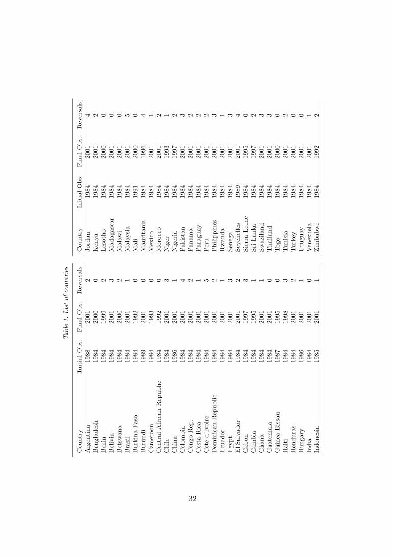
exist as soon as the dependent variable does not vary (as shown in Table 1, our
data set includes countries that never experienced a reversal).
Unobserved differences in the propensity to experience large reductions in
the current account deficit could also be serially correlated, rather than time-
invariant. As such they might reflect serially correlated shocks associated with
regional conflicts, uncertainty about government transition and political changes,
as well as regional commodity price shocks affecting the probability of experienc-
ing current account reversals. In order to take those effects into account, we
assume an AR(1) specification for the country specific transitory error compo-
nent.
Finally, unobserved and serially correlated transitory effects might also be
common to all countries reflecting either contagion effects or global shocks such
as oil or commodity price shocks. The former have received a lot of attention
following the currency crises of the 1990s which rapidly spread across emerging
countries (see, e.g., Edwards and Rigobon, 2002). A crisis in one country may
lead investors to withdraw their investments from other markets without taking
into account differences in economic fundamentals. In addition, a crisis in one
economy can also affect the fundamentals of other countries through trade links
and currency devaluations. Trading partners of a country in which a financial
6
crisis has induced a sharp currency depreciation could experience a deterioration
of the trade balance and current account resulting from a decline in exports and
an increase in imports (see Corsetti et al., 1999). In the words of the former
Managing Director of the IMF: “from the viewpoint of the international system,
the devaluations in Asia will lead to large current account surpluses in those
countries, damaging the competitive position of other countries and requiring
them to run current account deficit.” Fisher (1998).
Currency devaluations of countries that experience a crisis can often be seen
as a beggar-thy-neighbor policy in the sense that they incite output growth and
employment domestically at the expense of output growth, employment and cur-
rent account deficit abroad (Corsetti et al., 1999). Competitive devaluations also
happen in response to this process, as other economies may in turn try to avoid
competitiveness loss through devaluations of their own currency. This appears
to have happened during the East Asian crises in 1997 (Dornbusch et al., 2000).
If data are collected at short enough time intervals (monthly or quarterly
observations), such spill-over effects would become manifest in the dependence
of a country’s propensity to experience a reversal from lagged reversals by other
countries. However, with yearly data the time intervals are presumably not fine
enough to observe such short-run spill-over effects of one country on another and
contagion would more likely translate into a common time effect. Hence, we use
an AR(1) time-random effect which is common to all countries in order to account
for contagion effects together with global shocks.
3 The Data
Our data set consists of an unbalanced panel for 60 low and middle income
countries from Africa, Asia, and Latin America and the Caribbean. The complete
list of countries is given on Table 1. The time span of the data set ranges from
1975 to 2004, although the unavailability of some explanatory variables often
restrict the analysis to shorter time intervals. The minimum number of periods
for a country is 9, the maximum is 18 and the average is 16.5 for a total of 963
yearly observations. The initial values of the binary dependent variable indicating
the occurrence of a current account crisis are known for the initial time period
t = 0 for all countries. The sources of the data are the World Bank’s World
7

Development Indicators (2005) and the Global Development Finance (2004).
Current account reversals are defined as in Milesi-Ferretti and Razin (1998).
According to this definition a current account reversal has to meet three require-
ments. The first is an average reduction of the current account deficit of at least
3 percentage points of GDP over a period of 3 years relative to the 3-year average
before the event. The second requirement is that the maximum deficit after the
reversal must be no larger than the minimum deficit in the 3 years preceding the
reversal. The last requirement is that the average current account deficit over the
3-year period starting with the event must be less than 10% of GDP. According
to this definition we find current account reversals for 100 individual periods in
44 countries (10% of the total number of observations). Defining the duration of
a reversal episode as the number of consecutive periods with a reversal we observe
66 episodes with an average duration of 1.52 years and a maximal duration of 4
years (see Figure 3 below for a plot of the relative frequencies of the durations).
As discussed in Section 2.1, the selection of the explanatory variables follows
mainly the study of Milesi-Ferretti and Razin (1998). We include lagged macroe-
conomic, external, debt and foreign variables. The macroeconomic variables are
the annual growth rate of GDP (AVGGROW), the share of investment to GDP
proxied by the ratio of gross capital formation to GDP (AVGINV), government
expenditure (GOV) and interest payments relative to GDP (INTPAY). The ex-
ternal variables are the current account balance as a fraction of GDP (AVGCA),
a terms of trade index set equal to 100 for the year 2000 (AVGTT), the share of
exports and imports of goods and services to GDP as a measure of trade open-
ness (OPEN), the rate of official transfers to GDP (OT) and the share of foreign
exchange reserves to imports (RES). The debt variable we include is the share
of consessional debt to total debt (CONCDEB). Foreign variables such as the
US real interest rate (USINT) and the real growth rates of the OECD countries
(GROWOECD) are also included to reflect the influence of the world economy.
As in Milesi-Ferretti and Razin (1998), the current account, growth, investment
and terms of trade variables are 3-years averages, in order to ensure consistency
with the way reversals are measured.
8

4 Empirical Specifications
Our baseline specification consists of a dynamic panel probit model of the form
y∗it = x′itπ + κyit−1 + eit, yit = I(y∗it > 0), i = 1, ..., N, t = 1, ..., T, (2)
where I(y∗it > 0) is an indicator function that transforms the latent continuous
variable y∗it for country i in year t into the binary variable yit, indicating the oc-
currence of a current account reversal (yit = 1). The error term eit is assumed to
be normally distributed with zero mean and a fixed variance. Since Equation (2)
is only identified up to a positive multiplicative constant, a normalization condi-
tion will be required for each model variant (see Section 4.4 below). The vector
xit contains the observed macroeconomic, external, debt and foreign variables
which might affect the incidence of a reversal. The lagged dependent variable
on the right hand side captures possible state dependence. It implies that the
covariates in xit have not only a contemporaneous but also a persistent effect on
the probability of a reversal.
The most restrictive version of the panel probit assumes that the error eit
is independent across time and countries and imposes the restriction κ = 0.
This produces the standard pooled probit estimator which ignores possible serial
dependence and unobserved heterogeneity which cannot be attributed to the
variables in xit.
4.1 Random country-specific effects
In order to account for unobserved time invariant heterogeneity across countries
we consider the random effect model proposed by Butler and Moffitt (1982). It
assumes the following specification for the error term in Equation (2):
eit = τi + εit, εit ∼ i.i.d.N(0, 1), τi ∼ i.i.d.N(0, σ2τ ). (3)
The country-specific term τi captures potential permanent latent differences in
the propensity to experience a reversal. It is assumed that τi and εit are inde-
pendent from the variables included in xit. If, however, xit did contain variables
reflecting countries’ general susceptibility to current account crises, then τi would
be correlated with xit. We also assume that the observed initial states yi0 are
9
non-random constants. This assumption eliminates an ’initial condition problem’
due to correlation between τi and yi0 (see, e.g., Wooldridge, 2005). Since, how-
ever, ignoring correlation between τi and xit and yi0 would lead to inconsistent
estimates, we shall test below for such correlation.
Finally, note that the time-invariant heterogeneity component τi implies a con-
stant cross-period correlation of the error term eit which is given by corr(eit, eis)
= σ2τ/(σ
2τ + 1) for t 6= s (see, e.g., Greene, 2003).
The Butler-Moffitt model (2) and (3) can be estimated by ML. Let y =
{{yit}Tt=1}N
i=1, x = {{xit}Tt=1}N
i=1 and θ denote the parameter vector to be es-
timated. The likelihood function is given by L(θ; y, x) =∏N
i=1 Ii(θ), where Ii
represents the likelihood contribution of country i. The latter has the form
Ii(θ) =
∫
R1
T∏t=1
[Φyit
it (1− Φit)(1−yit)
]fτ (τi)dτi, (4)
where Φit = Φ(x′itπ + κyit−1 + τi), Φ denotes the cdf of the standardized normal
distribution and fτ the pdf of τi. In the application below, the one dimensional
integrals in τi are evaluated using a Gauss-Hermite quadrature rule (see, e.g.,
Butler and Moffitt, 1982).
Once the parameters have been estimated, the Gauss-Hermite procedure can
also be used to compute estimates of the random country-specific effects τi or
of functions thereof. Those estimates are instrumental for computing predicted
probabilities and average partial effects as well as for validating the orthogonality
conditions imposed on τi. Let g(τi) denote a function of τi. Its conditional
expectation given the complete sample information (y, x) obtains as
E[g(τi)|y, x; θ] =
∫R1 g(τi)h(y
i, τi|xi; θ)dτi∫
R1 h(yi, τi|xi; θ)dτi
, (5)
where h denotes the joint conditional pdf of yi
= {yit}Tt=1 and τi given xi =
{xit}Tt=1, as defined by the integrand of the likelihood (4). For the evaluation of
the numerator and denominator by Gauss-Hermite, the parameters θ are set to
their ML-estimates.
Estimates τi of the random effects obtain by setting g(τi) = τi in Equation
(5). An auxiliary regression of those estimates against the time average of the ex-
10
planatory variables and the initial conditions provides a direct test of the validity
of the orthogonality condition between τi and (xi, yi0).
Next, in order to obtain predicted probabilities and average marginal effects
we consider the conditional response probability
p(yit = 1|xit, yit−1, τi) = Φ(x′itπ + κyit−1 + τi), (6)
and its partial derivative w.r.t. the kth (continuous) variable in xit
∂xitkp(yit = 1|xit, yit−1, τi) = πkφ(x′itπ + κyit−1 + τi), (7)
where φ denotes the standardized Normal density and πk the regression coefficient
of the covariate xitk. Both expressions represent functions of τi, which can be
averaged across the conditional distribution of τi given the sample information
(y, x), according to Equation (5). The average marginal effect of the kth covariate
then obtains as the sample mean across i and t of the averaged partial derivatives
(7). Analogously, we compute the average partial effect of the binary lagged
dependent variable as the sample mean of the differences in the probabilities
p(yit = 1|xit, yit−1 = 1, τi) and p(yit = 1|xit, yit−1 = 0, τi) averaged across the
conditional distribution of τi given (y, x).
4.2 Serially correlated country-specific errors
We generalize the random effect specification introduced in Section 4.1 by as-
suming that εit in Equation (3) follows an idiosyncratic AR(1) process, capturing
persistent country-specific shocks and omitted macroeconomic or political factors.
Accordingly, Equation (3) is generalized into
eit = τi + εit, εit = ρεit−1 + ηit, ηit ∼ i.i.d.N(0, 1), (8)
where τi and ηit are mutually independent. As before, they are also assumed to
be independent from the variables included in xit and yi0. In order to ensure
stationarity we assume that |ρ| < 1.
The computation of the likelihood contribution Ii(θ) for model (3) and (8) now
requires the evaluation of (T + 1)-dimensional integrals. Let λ′it = (εit, εit−1, τi),
λ′i1 = (εi1, τi), and λ′i = (τi, εi1, ..., εiT ). Under the assumption that εi0 = 0, the
11
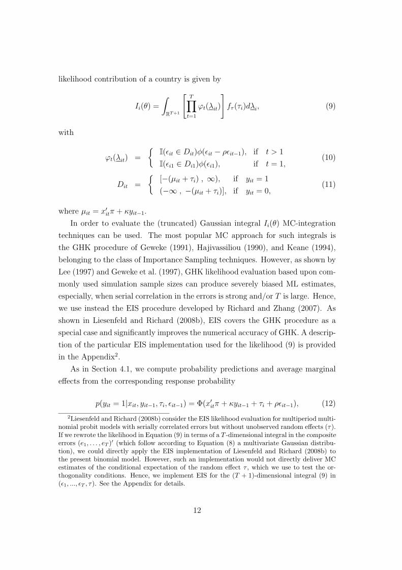
likelihood contribution of a country is given by
Ii(θ) =
∫
RT+1
[T∏
t=1
ϕt(λit)
]fτ (τi)dλi, (9)
with
ϕt(λit) =
{I(εit ∈ Dit)φ(εit − ρεit−1), if t > 1
I(εi1 ∈ Di1)φ(εi1), if t = 1,(10)
Dit =
{[−(µit + τi) , ∞), if yit = 1
(−∞ , −(µit + τi)], if yit = 0,(11)
where µit = x′itπ + κyit−1.
In order to evaluate the (truncated) Gaussian integral Ii(θ) MC-integration
techniques can be used. The most popular MC approach for such integrals is
the GHK procedure of Geweke (1991), Hajivassiliou (1990), and Keane (1994),
belonging to the class of Importance Sampling techniques. However, as shown by
Lee (1997) and Geweke et al. (1997), GHK likelihood evaluation based upon com-
monly used simulation sample sizes can produce severely biased ML estimates,
especially, when serial correlation in the errors is strong and/or T is large. Hence,
we use instead the EIS procedure developed by Richard and Zhang (2007). As
shown in Liesenfeld and Richard (2008b), EIS covers the GHK procedure as a
special case and significantly improves the numerical accuracy of GHK. A descrip-
tion of the particular EIS implementation used for the likelihood (9) is provided
in the Appendix2.
As in Section 4.1, we compute probability predictions and average marginal
effects from the corresponding response probability
p(yit = 1|xit, yit−1, τi, εit−1) = Φ(x′itπ + κyit−1 + τi + ρεit−1), (12)
2Liesenfeld and Richard (2008b) consider the EIS likelihood evaluation for multiperiod multi-nomial probit models with serially correlated errors but without unobserved random effects (τ).If we rewrote the likelihood in Equation (9) in terms of a T -dimensional integral in the compositeerrors (e1, . . . , eT )′ (which follow according to Equation (8) a multivariate Gaussian distribu-tion), we could directly apply the EIS implementation of Liesenfeld and Richard (2008b) tothe present binomial model. However, such an implementation would not directly deliver MCestimates of the conditional expectation of the random effect τ , which we use to test the or-thogonality conditions. Hence, we implement EIS for the (T + 1)-dimensional integral (9) in(ε1, ..., εT , τ). See the Appendix for details.
12
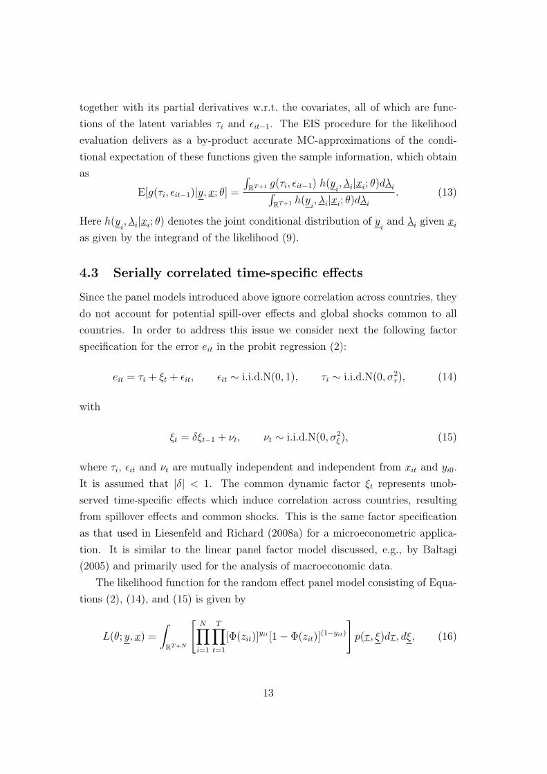
together with its partial derivatives w.r.t. the covariates, all of which are func-
tions of the latent variables τi and εit−1. The EIS procedure for the likelihood
evaluation delivers as a by-product accurate MC-approximations of the condi-
tional expectation of these functions given the sample information, which obtain
as
E[g(τi, εit−1)|y, x; θ] =
∫RT+1 g(τi, εit−1) h(y
i, λi|xi; θ)dλi∫
RT+1 h(yi, λi|xi; θ)dλi
. (13)
Here h(yi, λi|xi; θ) denotes the joint conditional distribution of y
iand λi given xi
as given by the integrand of the likelihood (9).
4.3 Serially correlated time-specific effects
Since the panel models introduced above ignore correlation across countries, they
do not account for potential spill-over effects and global shocks common to all
countries. In order to address this issue we consider next the following factor
specification for the error eit in the probit regression (2):
eit = τi + ξt + εit, εit ∼ i.i.d.N(0, 1), τi ∼ i.i.d.N(0, σ2τ ), (14)
with
ξt = δξt−1 + νt, νt ∼ i.i.d.N(0, σ2ξ ), (15)
where τi, εit and νt are mutually independent and independent from xit and yi0.
It is assumed that |δ| < 1. The common dynamic factor ξt represents unob-
served time-specific effects which induce correlation across countries, resulting
from spillover effects and common shocks. This is the same factor specification
as that used in Liesenfeld and Richard (2008a) for a microeconometric applica-
tion. It is similar to the linear panel factor model discussed, e.g., by Baltagi
(2005) and primarily used for the analysis of macroeconomic data.
The likelihood function for the random effect panel model consisting of Equa-
tions (2), (14), and (15) is given by
L(θ; y, x) =
∫
RT+N
[N∏
i=1
T∏t=1
[Φ(zit)]yit [1− Φ(zit)]
(1−yit)
]p(τ , ξ)dτ , dξ, (16)
13
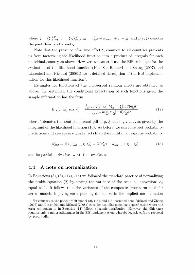
where ξ = {ξt}Tt=1, τ = {τi}N
i=1, zit = x′itπ + κyit−1 + τi + ξt, and p(τ , ξ) denotes
the joint density of τ and ξ.
Note that the presence of a time effect ξt common to all countries prevents
us from factorizing the likelihood function into a product of integrals for each
individual country as above. However, we can still use the EIS technique for the
evaluation of the likelihood function (16). See Richard and Zhang (2007) and
Liesenfeld and Richard (2008a) for a detailed description of the EIS implemen-
tation for this likelihood function3.
Estimates for functions of the unobserved random effects are obtained as
above. In particular, the conditional expectation of such functions given the
sample information has the form
E[g(τi, ξt)|y, x; θ] =
∫RN+T g(τi, ξt) h(y, τ , ξ|x; θ)dξdτ∫
RN+T h(y, τ , ξ|x; θ)dξdτ, (17)
where h denotes the joint conditional pdf of y, ξ and τ given x, as given by the
integrand of the likelihood function (16). As before, we can construct probability
predictions and average marginal effects from the conditional response probability
p(yit = 1|xit, yit−1, τi, ξt) = Φ(x′itπ + κyit−1 + τi + ξt), (18)
and its partial derivatives w.r.t. the covariates.
4.4 A note on normalization
In Equations (3), (8), (14), (15) we followed the standard practice of normalizing
the probit equation (2) by setting the variance of the residual innovations εit
equal to 1. It follows that the variances of the composite error term eit differ
across models, implying corresponding differences in the implicit normalization
3In contrast to the panel probit model (2), (14), and (15) assumed here, Richard and Zhang(2007) and Liesenfeld and Richard (2008a) consider a similar panel logit specification where theerror component εit in Equation (14) follows a logistic distribution. However, this differencerequires only a minor adjustment in the EIS implementation, whereby logistic cdfs are replacedby probit cdfs.
14
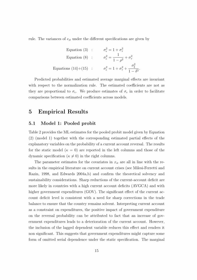
rule. The variances of eit under the different specifications are given by
Equation (3) : σ2e = 1 + σ2
τ
Equation (8) : σ2e =
1
1− ρ2+ σ2
τ
Equations (14)+(15) : σ2e = 1 + σ2
τ +σ2
ξ
1− δ2.
Predicted probabilities and estimated average marginal effects are invariant
with respect to the normalization rule. The estimated coefficients are not as
they are proportional to σe. We produce estimates of σe in order to facilitate
comparisons between estimated coefficients across models.
5 Empirical Results
5.1 Model 1: Pooled probit
Table 2 provides the ML estimates for the pooled probit model given by Equation
(2) (model 1) together with the corresponding estimated partial effects of the
explanatory variables on the probability of a current account reversal. The results
for the static model (κ = 0) are reported in the left columns and those of the
dynamic specification (κ 6= 0) in the right columns.
The parameter estimates for the covariates in xit are all in line with the re-
sults in the empirical literature on current account crises (see Milesi-Ferretti and
Razin, 1998, and Edwards 2004a,b) and confirm the theoretical solvency and
sustainability considerations. Sharp reductions of the current-account deficit are
more likely in countries with a high current account deficits (AVGCA) and with
higher government expenditures (GOV). The significant effect of the current ac-
count deficit level is consistent with a need for sharp corrections in the trade
balance to ensure that the country remains solvent. Interpreting current account
as a constraint on expenditures, the positive impact of government expenditure
on the reversal probability can be attributed to fact that an increase of gov-
ernment expenditures leads to a deterioration of the current account. However,
the inclusion of the lagged dependent variable reduces this effect and renders it
non significant. This suggests that government expenditures might capture some
form of omitted serial dependence under the static specification. The marginal
15
effect of foreign reserve (RES) is negative and significant which suggests that low
levels of reserves make it more difficult to sustain a large trade imbalance and
may also reduce foreign investors’ willingness to lend (Milesi-Ferretti and Razin,
1998). Also, reversals seem to be less common in countries with a high share
of concessional debt (CONCDEB). This would be consistent with the fact that
concessional debts tend to be higher in countries which have difficulties reducing
external imbalances. Finally, countries with a lower degree of openness (OPEN),
weaker terms of trade (AVGTT) and higher GDP growth (AVGGROW) seem
to face higher probabilities of reversals, especially when growth rate in OECD
countries (GROWOECD) and/or US interest rate (USINT) are higher – though
none of these five coefficients are statistically significant.
Note that the size of the estimated marginal effects for the significant eco-
nomic covariates on the probability of reversals are typically fairly small, ranging
from 0.004 to 0.026. Nevertheless, they are far from being negligible when ap-
plied to the low unconditional probability of experiencing a reversal which is
approximately 0.1.
The inclusion of the lagged current account reversal variable substantially
improves the fit of the model as indicated by the significant increase of the max-
imized log-likelihood value. The estimated coefficient κ measuring the impact of
the lagged dependent state variable is positive and significant at the 1% signif-
icance level with a large estimated partial effect of 0.21. This suggests that a
current account reversal significantly increases the probability of a further rever-
sal the following year. This would be consistent with the hypothesis that reversal
processes stretch over more than a year due to slow adjustments in international
trade flows (see, Junz and Rhomberg, 1973, and Himaraios, 1989).
In order to analyze the dynamic effects of a covariate xitk implied by the
model with lagged dependent variable we use the sample average of the l-step
ahead marginal effect, i.e.,
1
N(T − `)
N∑i=1
T−∑t=1
∂xitkp(yit+` = 1|xit+`, ..., xit, yit−1), ` = 1, 2, ... . (19)
The probability p(yit+` = 1|xit+`, ..., xit, yit−1) is obtained by considering the event
tree associated with all possible yit-trajectories starting in period t and ending in
period t+ ` with yit+` = 1. Analogously, the dynamic effects of the state variable
16

is measured by
1
N(T − `)
N∑i=1
T−∑t=1
[p(yit+` = 1|xit+`, ..., xit+1, yit = 1) (20)
−p(yit+` = 1|xit+`, ..., xit+1, yit = 0)], ` = 1, 2, ... .
The upper left panel of Figure 1 plots the dynamic marginal effects for the sig-
nificant covariates (AVGCA, RES, CONCDEB) and the lagged state variable for
` = 1, ..., 4, respectively. It reveals substantial long-run effects of the state vari-
able, whereby the occurrence of a current account reversal increases a country’s
propensity to experience further large reductions in the current account in subse-
quent years. This effect appears to stretch over a two-to-three-year period. This
would be in line with the result of Himarios (1989) showing that changes in trade
flows triggered by currency devaluations often used to correct the trade balance
are distributed over a time span of a about two or three years. However, note
that this long-run state dependence does not translate into significant long-run
effects of the covariates AVGCA, RES, and CONCDEB which is consistent with
the fact that their contemporaneous effects reported in Table 2 are already fairly
small.
5.2 Model 2: Random country-specific effects
Table 3 reports the estimates of the dynamic Butler-Moffitt model with random
country specific effects as specified by Equations (2) and (3) (model 2). The
ML-estimates are obtained using a 20-points Gauss-Hermite quadrature. The
estimate of the coefficient στ indicates that only 3% of the total variation in the
latent error is due to unobserved country-specific heterogeneity and this effect
is not statistically significant. Nevertheless, the maximized log-likelihood of the
random effect model is significantly larger than that of the dynamic pooled probit
model with a likelihood-ratio (LR) test statistic of 5.57. Since the parameter value
under the Null hypothesis στ = 0 lies at the boundary of the admissible parameter
space, the distribution of the LR-statistic under the Null is a (0.5χ2(0) + 0.5χ2
(1))-
distribution, where χ2(0) represents a degenerate distribution with all its mass at
origin (see, e.g., Harvey, 1989). Whence, the critical value for a significance level
of 1% is the 0.98-quantile of a χ2(1)-distribution which equals 5.41. All in all, the
17
evidence in favor of the random effect specification for time-invariant differences
of institutional, political, and economic factors across countries is borderline.
Actually, the marginal effects as well as the predicted dynamic effects (see, upper
right panel of Figure 1) obtained under the random country-specific effect model
are very similar to those for the dynamic pooled model.
In order to check the assumption that τi is independent of xit and yi0 we ran
the following auxiliary regression:
τi = ψ0 + x′i·ψ1 + yi0ψ2 + ζi, i = 1, ..., n, (21)
where the vector xi· contains the mean values of the xit-variables over time (except
for the US interest rate and the OECD growth rate). The value of the F -statistic
for the null ψ1 = 0 is 1.94 with critical values of 2.71 and 2.03 for the 1% and 5%
significance levels. The absolute value of the t-statistic for the null ψ2 = 0 is 2.01
with critical values of 2.68 and 2.01 for the 1% and 5% levels. Whence, evidence
that τi might be correlated with xi· and yi0 is inconclusive.
5.3 Model 3: AR(1) country-specific errors
We now turn to the ML-EIS estimates of the dynamic random effect model with
AR(1) idiosyncratic errors (model 3) as specified by Equations (2) and (8). It
ought to capture possible serially correlated shocks associated with regional politi-
cal changes or conflicts and persistent local macroeconomic events like commodity
price shocks. The ML-EIS estimation results based on a simulation sample size
of S = 100 are given in the left columns of Table 4 4.
The results indicate that the inclusion of a country-specific AR(1) error com-
ponent has significant effects on the dynamic structure of the model but only a
slight impact on the marginal effects of the xit-variables, which remain typically
very close to those of the pure random country-specific effect model in Table 3.
An exception is the effect of the terms of trade (AVGTT) which becomes signifi-
4We also estimated the parameters of model 3 using the standard GHK procedure based onS = 100. The comparison of those estimates (not provided here) with the ML-EIS estimatesprovided in Table 4 reveal that the parameter estimates for the explanatory variables aregenerally similar for both procedures. However, the estimates of the parameters governing thethe dynamics (κ, στ , ρ) are noticeably different. This is fully in line with results of the MC-studyof Lee (1997), indicating that the ML-GHK estimates of those parameters are often severelybiased.
18
cant at the 10% level. Also, while the parameter στ governing the time-invariant
heterogeneity remains statistically insignificant, the estimated coefficient κ asso-
ciated with the lagged dependent variable and its partial effect are now much
smaller. This leads to a substantial attenuation of the long-run effect of the
lagged state variable (see lower left panel of Figure 1). The estimate of the per-
sistence parameter of the AR(1) error component ρ equals 0.35 and is statistically
significant at the 10% level. However, the corresponding LR-statistic equals 2.40
and is not significant. Hence, despite its impact on the dynamic structure of the
model, the inclusion of an AR(1) error component does not significantly improve
the overall fit.
Since a lagged dependent variable and a country-specific AR(1) error com-
ponent can generate similar looking patterns of persistence in the dependent
variable, these results suggest that the AR(1) error captures some of the serial
dependence which is captured by the lagged dependent variable under the pooled
probit and the pure random country-specific effect model. However, the small
likelihood improvement obtained by the inclusion of an AR(1) error together with
the fairly large standard errors of the estimates for κ and ρ suggest that the model
has difficulties separating these two sources of serial dependence. In order to ver-
ify this conjecture, we re-estimated the model with the AR(1) country-specific
error component without state-dependence. The ML-EIS results are provided
in the right columns of Table 4 and confirm our conjecture. In fact, the esti-
mated AR coefficient ρ increases to 0.59 and is now highly significant according
to both the t- and LR-test statistics, while the maximized likelihood value are not
significantly different from those obtained for the models including either state-
dependence only (Table 3) or both state-dependence and an AR error component
(left columns of Table 4).
All in all, our results indicate that the data are ambiguous on the question
of whether the observed persistence in current account reversals is due to state
dependence associated with the hypothesis of slow adjustments in international
trade flows or due to serially correlated country-specific shocks related to local
political or macroeconomic events.
19
5.4 Model 4: AR(1) time-specific effects
We now turn to the estimation results of the dynamic panel model given by
Equations (2), (14), and (15), allowing for unobserved random time-specific ef-
fects designed to capture potential spill-over effects and/or global shocks common
to all countries (model 4). The ML-EIS estimation results obtained using a sim-
ulation sample size of S = 100 are summarized in Table 5.
The estimated marginal effects for all explanatory xit-variables and the esti-
mated variance parameter στ of the time-invariant heterogeneity are very similar
to those obtained under the models discussed above. Here again, we find no
conclusive evidence for correlation between τi and (xi·, yi0). The results show a
large and highly significant state-dependence effect similar to that found under
the pure random country-specific effect model in Table 3. The variance param-
eter of the time factor σξ and its autoregressive parameter δ are both highly
significant, indicating that there are significant common dynamic time-specific
effects in addition to state dependence. Hence, in contrast to the specification
with state dependence and an AR country-specific error component, the model
seems to be able to separate the two sources of persistence. Also, the estimated
autocorrelation parameter of -0.89 implies a strong mean reversion in the com-
mon time-specific factor. This mean-reverting tendency in the common factor
affects the common probability of experiencing a current account reversal across
all countries and is, therefore, fully consistent with a global accounting restriction
requiring that deficits and surpluses across all national current accounts need to
be balanced. In particular, one would expect that a temporary simultaneous
increase in the propensities to experience a large reduction in current account
deficits is immediately reverted in order to guarantee a global balance in deficits
and surpluses, rather than a persistent and long-lasting increase in individual
propensities.
Although the time-specific factor capturing global shocks and/or contagion
effects is significant, it appears to be quantitatively fairly small. In fact, the
fraction of error variance due to the time-specific effect in only 3.5%. Therefore,
it is not surprising that the overall fit of the model and its predicted dynamic
effects (see, the lower right panel of Figure 1) do not change significantly relative
to the pure random country-specific effect model in Table 3 which leaves out the
time-specific effect.
20
Finally, we note that the quantitatively low impact of the common time-
specific factor might be due to the implicit restriction that the loading w.r.t. that
factor is the same across all countries. Hence, a natural extension of the model
would be to allow for factor loadings, which differ across countries (whether
randomly or deterministically). However, due to a substantial increase in the
number of parameters or the dimension of the integration problem associated
with the likelihood evaluation the statistical inference of such an extension is
non-trivial without further restrictions and is left to future research.
6 Predictive Performance
Models 2 to 4 are essentially observationally equivalent with log-likelihood values
ranging from -253.1 to -255.2. However, log-likelihood comparisons provide an
incomplete picture of the overall quality of a binary model. Hence, we compare
next models 2 to 4 on two predictive benchmarks: the proportion of correctly pre-
dicted binary outcomes and predicted duration distribution of reversal episodes.
Assessing the predictive performance of an estimated binary model requires
selecting a threshold c whereby success (current account reversal) is predicted
iff the predicted probability is larger than c, i.e., rit = p(yit|xit, yit−1) > c. The
corresponding classification error probabilities are given by
α(c) = 1− p(rit > c|yit = 1) and β(c) = p(rit > c|yit = 0), (22)
which can be approximated by the corresponding relative frequencies of misclas-
sification. Since the sample portion Π of success is only of the order of 0.1, it does
not make sense to select a threshold c which minimizes the unconditional proba-
bility of misclassification p(c) = Πα(c)+(1−Π)β(c). Following Winkelmann and
Boes (2006), we first computed for each model the threshold c∗ which minimizes
the sum of classification error probabilities α(c) + β(c). We also computed their
Receiver Operating Characteristic (ROC) curves, defined as the curves plotting
1− α(c) against β(c), as well as the areas under these ROC curves. These areas
have a minimum of 0.5 (complete randomness) and a maximum of 1 (errorless
classification). The ROC curves are displayed in Figure 2 and associated results
for the optimal threshold c∗, classification error probabilities for c∗ and ROC
areas are reported in Table 6.
21
Note that c∗ ranges from 0.08 to 0.11, which are close to the sample proportion
Π of 0.10. Model 3 with AR(1) country-specific errors without state-dependence
has the best predictive performance with α(c∗) + β(c∗) = 0.27 and a ROC area
of 0.91 (the corresponding figures for the other models range from 0.36 to 0.43
and 0.85 to 0.88, respectively). Also its ROC curve dominates those of the other
models. Based on the optimal threshold it correctly predicts 91% of the observed
reversals and 82% of the non-reversals.
We also used each estimated model to simulate 20,000 fictitious panel data
sets of the binary outcome conditional on the observed xit variables in order to
obtain accurate MC approximations of the predictive distributions of the duration
of reversal episodes to be compared with the frequency distribution observed for
the data (see Figure 3, and Table 6 for predicted average durations). It appears
that models 2 and 4 have a better performance than model 3 with a better
fit to the empirical distribution and predicted average durations closer to the
observed average of 1.52. However, the differences across the models seem to be
not large enough to overturn the ROC ranking. Thus, if the likelihood criterion,
which by itself is fairly uninformative about the source of serial dependence,
is supplemented by measures of predictive performance, the model with AR(1)
country-specific shocks and without state-dependence appears to be the preferred
specification.
7 Conclusion
This paper uses different non-linear panel data specifications in order to inves-
tigate the causes and dynamics of current account reversals in low- and middle-
income countries. In particular, we analyze four sources of serial persistence:
(i) a country-specific random effect reflecting time-invariant differences in in-
stitutional, political or economic factors; (ii) serially correlated transitory error
component capturing persistent country-specific shocks; (iii) dynamic common
time-specific factor effects, designed to account for potential spill-over effects and
global shocks to all countries; and (iv) a state dependence component to control
for the effect of previous events of current account reversal and to capture slow
adjustments in international trade flows.
The likelihood evaluation of the panel models with country-specific random
22
heterogeneity and serially correlated error components requires high-dimensional
integration for which we use a generic Monte-Carlo integration technique known
as Efficient Importance Sampling (EIS).
Our empirical results indicate that the static pooled probit model is strongly
dominated by the alternative models with serial dependence. However, state-
dependence and transitory country-specific errors are essentially observationally
equivalent. Only if we include random time-specific effects into the model with
state-dependence, we find that both sources of serial dependence are significant,
even though the time-specific effect is small with limited effect on the overall fit
of the model. On the other hand, our assessment of the ability to predict current
account reversals provides strong support for the model with transitory country-
specific errors and without state-dependence, which appears to present the best
compromise between log-likelihood fit and predictive performance. Also, we do
not find conclusive evidence for the existence of random country-specific effects.
Overall, our results relative to the determinants of current account reversals
are in line with the those in the empirical literature on current account crises
and confirm the empirical relevance of theoretical solvency and sustainability
considerations w.r.t. a country’s trade balance. In particular, countries with high
current account imbalances, low foreign reserves, a small fraction of concessional
debt, and unfavorable terms of trades are more likely to experience a current
account reversal. These results are fairly robust against the dynamic specification
of the model.
Acknowledgement
We are grateful to an anonymous referee for his helpful comment which have pro-
duced major clarifications on several key issues. Roman Liesenfeld and Guilherme
V. Moura acknowledge research support provided by the Deutsche Forschungsge-
meinschaft (DFG) under grant HE 2188/1-1; Jean-Francois Richard acknowledges
the research support provided by the National Science Foundation (NSF) under
grant SES-0516642.
23
Appendix: EIS for random effects and serially
correlated errors
This appendix details the implementation of the EIS procedure for the panel
probit model (2) and (8) to obtain MC estimates for the likelihood contribution
Ii(θ) given by equation (9) (for a detailed description of the EIS principle, see
Richard and Zhang, 2007). In order to simplify the following presentation it
proves convenient to omit the country index i and to relabel τ as λ0. Then the
likelihood integral in Equation (9) can be rewritten as
I(θ) =
∫
RT+1
T∏t=0
ϕt(λt)dλ, (A-1)
where ϕ0(λ0) = fτ (τ). Next, we partition λ′t into (εt, η′t−1
) with η′t−1
= (εt−1, λ0)
for t > 1, η0 = λ0 and η−1 = ∅. EIS is based upon a sequence of auxiliary
importance sampling densities of the form
mt(εt|ηt−1; at) =
kt(λt; at)
χt(ηt−1; at)
, with χt(ηt−1; at) =
∫
R1
kt(λt; at)dεt, (A-2)
for t = 0, ...., T , where {kt(λt; at); at ∈ At} denotes a (pre-selected) class of aux-
iliary parametric density kernels with analytical integrating factor in εt given
(ηt−1
, at) denoted by χt(ηt−1; at).
Let {λ(j)= {λ(j)
t }Tt=0}S
j=1 be S independent trajectories drawn from the auxil-
iary sampler m(λ|a) =∏T
t=0 mt(εt|ηt−1; at). The corresponding Importance Sam-
pling MC estimate of I(θ) obtains as:
IS(θ) = χ0(a0)1
S
S∑j=1
T∏t=0
ϕt(λ(j)
t )χt+1(η(j)
t; at+1)
kt(λ(j)
t ; at)
. (A-3)
An Efficient Importance Sampler is one which minimizes the MC sampling vari-
ances of the ratios ϕtχt+1/kt w.r.t. the auxiliary parameters {at}Tt=0 under such
draws. An approximate solution to this minimization problem, say {at}Tt=0, ob-
tains by a sequence of T + 1 back recursive regressions. In particular, in each
24
period t = T, ..., 0 one needs to regress
ln[ϕt(λ(j)
t )χt+1(η(j)
t; at+1)] on: intercept, ln kt(λ
(j)
t , at), (A-4)
where {λ(j)}Sj=1 are drawn from an initial sampler m(λ|a0). As an initial sam-
pler we use the GHK sampling densities and the EIS sequence is iterated until
obtainment of a fixed point in {at}Tt=0.
The kernel kt(λt; at) in Equation (A-2) is selected to be a parametric extension
of the period-t integrand ϕt in Equation (A-1). The latter includes a (truncated)
Gaussian kernel in λt. Hence, kt is specified as
kt(λt; at) = ϕt(λt) · ζt(λt; at), (A-5)
where ζt is itself a gaussian kernel in λt. It follows that ϕt cancels out in the EIS
regression (A-4). For the truncated Gaussian kernel kt given in Equation (A-5)
we use the following parametrization:
kt(λt; at) =I(εt ∈ D∗
t )√2π
exp{−1
2(λ′tPtλt + 2λ′tqt)}, (A-6)
where D∗t = (−∞ , γt + δtλ0], with γt = (2yt − 1)µt and δt = (2yt − 1). The
EIS parameter at consists of the six lower diagonal elements of Pt and the three
elements in qt. In what follows we make use of the Cholesky decomposition of Pt
into
Pt = Lt∆tL′t, (A-7)
where Lt = {lij,t} is a lower triangular matrix with ones on the diagonal and ∆t
is diagonal matrix with diagonal elements di,t ≥ 0. Let
l1,t = (l21,t, l31,t)′, l2,t = (1, l32,t)
′. (A-8)
The key step in our EIS implementation consists of finding the analytical expres-
sion of the integrating factor χt(ηt−1; at) associated with the density kernel (A-6).
It is the object of the following lemma.
25
Lemma 1. The integral of kt(λt; at) w.r.t. εt is of the form
χt(ηt−1; at) = k2,t(λ0; at)[Φ(αt + β′tηt−1
) · k1,t(ηt−1; at)], (A-9)
together with
k1,t(ηt−1; ·) = exp{−1
2(d2,tη
′t−1
l2,tl′2,tηt−1
+ 2η′t−1
l2,tm2,t)}, (A-10)
k2,t(λ0; ·) = exp{−1
2(d3,tλ
20 + 2m3,tλ0)} · rt, (A-11)
where
αt =√
d1,t(γt +m1,t
d1,t
), βt =√
d1,t(l1,t + δtι), (A-12)
rt =1√d1,t
exp{1
2
m21,t
d1,t
}, mt = {mi,t} = L−1
t qt, ι′ = (0, 1). (A-13)
Proof. The proof is straightforward under the Cholesky factorization introduced
in (A-7), deleting the index t for the ease of notation. First we introduce the
transformation z = L′λ, whereby z1 = ε + l′1η−1, z2 = l′2η−1
, and z3 = λ0.
Whence,
χ(η−1; ·) = exp
{− 1
2
3∑i=2
(diz2i + 2mizi)
}
× 1√2π
∫
D∗∗t
exp{−1
2(d1z
21 + 2m1z1)}dz1,
where D∗∗t = (−∞ , γt +(l1,t +δtι)
′η−1]. Next, we complete the quadratic form in
z1 under the integral sign and introduce the transformation v =√
d1[z1+(m1/d1)].
The result immediately follows.2
Next, we provide the full details of the recursive EIS implementation.
· Period t = T : With χT+1 ≡ 1, the only component of kT is ϕT itself.
Whence,
PT = eρe′ρ and qT = 0, with e′ρ = (1,−ρ, 0). (A-14)
· Period t (T > t > 1): Given Equation (A-9) in lemma 1, the product ϕt ·χt+1
comprises the following factors: ϕt as defined in Equation (10), k1,t+1 as given by
26
Equation (A-10) and Φ(αt+1 +β′t+1ηt), where (αt+1, βt+1) are defined in Equation
(A-12). The first two factors are already gaussian kernels. Furthermore, the term
Φ(·) depends on λt only through the linear combination β′t+1ηt. Whence, ζt in
Equation (A-5) is defined as
ζt(λt; at) = k1,t+1(ηt, ·) exp
{− 1
2
[a1,t(β
′t+1ηt
)2 + 2a2,t(β′t+1ηt
)]}
, (A-15)
with at = (a1,t, a2,t). It follows that k1,t+1 also cancels out in the auxiliary EIS
regressions (A-4) which simplifies into OLS of ln Φ(αt+1 + β′t+1ηt) on β′t+1ηt
and
(β′t+1ηt)2 together with a constant. From these EIS regressions one obtains esti-
mated EIS values for (a1,t, a2,t). Note that ηtcan be written as
ηt= Aλt, with A =
(1 0 0
0 0 1
). (A-16)
It follows that the parameters of the EIS kernel kt in Equation (A-6) are given
by
Pt = eρe′ρ + d2,t+1A
′l2,t+1l′2,t+1A + a1,tA
′βt+1β′t+1A (A-17)
qt = A′l2,t+1m2,t+1 + a2,tA′βt+1. (A-18)
Its integrating factor χt(ηt; at) follows by application of lemma 1.
· Period t = 1: The same principle as above applies to period 1, but requires
adjustments in order to account for the initial condition. Specifically, we have
λ1 = η1
= (ε1, λ0)′, λ0 = η0 (= τ). This amounts to replacing A by I2 in
Equations (A-16) to (A-18). Whence, the kernel k1(λ1, a1) needs only be bivariate
with
P1 = e1e′1 + d2,2l2,2l
′2,2 + a1,1β2β
′2 (A-19)
q1 = l2,2m2,2 + a2,1β2, (A-20)
with e′1 = (1, 0). Essentially, P1 and q1 have lost their middle row and/or column.
To avoid changing notation in lemma 1, the Cholesky decomposition of P1 is
27
parameterized as
L1 =
(1 0
l31,1 1
), D1 =
(d1,1 0
0 d3,1
), l1,1 = l31,1, (A-21)
while d2,2 and l2,2 are now zero. Under these adjustments in notation, lemma 1
still applies with k2(η0; ·) ≡ 1 and β1 reduced to the scalar
β1 =√
d1,1(l1,1 + δ1). (A-22)
· Period t = 0 (untruncated integral w.r.t. λ0 ≡ τ): Accounting for the back
transfer of {k2,t(λ0; ·)}Tt=1, all of which are gaussian kernels, the λ0-kernel is given
by
k0(λ0; ·) = fτ (λ0) ·T∏
t=1
k2,t(λ0; ·) · exp{−1
2
(a1,0λ
20 + 2a2,0λ0
)}, (A-23)
where (a1,0, a2,0) are the coefficients of the EIS approximation of ln Φ(α1 +β1λ0).
Note that k0 is the product of T +2 gaussian kernels in λ0 and is, therefore, itself
a gaussian kernel, whose mean m0 and variance v20 trivially obtain by addition
from Equation (A-23).
28
References
Baltagi, B., 2005. Econometric Analysis of Panel Data. John Wiley & Sons.
Butler, J.S., Moffitt, R., 1982. A computationally efficient quadrature procedure for
the one-factor multinomial probit model. Econometrica 50, 761–764.
Calvo, G., Izquierdo, A., Mejia, L.F., 2004. On the empirics of sudden stops: the
relevance of balance-sheet effects. Working paper. Inter-American Development
Bank.
Corsetti, G., Pesenti, P., Roubini, N., Tille, C. 1999. Competitive devaluations: a
welfare-based approach. NBER-Working Paper No 6889.
Dornbusch, R., Park, Y.C., Claessens, S., 2000. Contagion: Understanding how it
spreads. World Bank Research Observer 15, 177–197.
Edwards, S., 2004a. Financial openness, sudden stops and current account reversals.
American Economic Review 94, 59-64.
Edwards, S., 2004b. Thirty years of current account imbalances, current account
reversals, and sudden stops. NBER-Working Paper No. 10276.
Edwards, S., Rigobon, R. 2002. Currency crises and contagion: an introduction.
Journal of Development Economics 69, 307–313.
Eichengreen, B., Rose, A., Wyplosz 1995. Exchange rate mayhem: the antecedents
and aftermath of speculative attacks. Economic Policy 21, 249–312.
Falcetti, E., Tudela, M., 2006. Modelling currency crises in emerging markets: a
dynamic probit model with unobserved heterogeneity and autocorrelated errors.
Oxford Bulletin of Economics and Statistics 68, 445–471.
Fisher, S., 1998. The IMF and the asian crisis. Los Angeles, March 20.
Frankel, J., Rose, A., 1996. Currency crashes in emerging markets: an empirical treat-
ment. Board of Governors of the Federal Reserve System Oxford, International
Finance Diskussion Papers 534, 1–28.
Geweke, J., 1991. Efficient simulation from the multivariate normal and student-
t distributions subject to linear constraints. Computer Science and Statistics:
Proceedings of the Twenty-Third Symposium on the Interface, 571–578.
29
Geweke, J., Keane, M., 2001. Computationally intensive methods for integration
in econometrics. In Heckman, J., Leamer, E., Handbook of Econometrics 5,
Chapter 56. Elsevier.
Geweke, J., Keane, M., Runkle, D. 1997. Statistical inference in the multinomial
multiperiod probit model. Journal of Econometrics 80, 125–165.
Greene, W., 2003. Econometrics Analysis. Prentice Hall, Englewood Cliffs.
Greene, W., 2004. Convenient estimators for the panel probit model: further results.
Empirical Economics 29, 21–47.
Hajivassiliou, V., 1990. Smooth simulation estimation of panel data LDV models.
Mimeo. Yale University.
Harvey, A., 1989. Forecasting, Structural Time Series Models and Kalman Filter.
Cambridge University Press.
Heckman, J., 1981. Statistical models for discrete panel data. In Manski, C.F., Mc-
Fadden, D., Structural Analysis of Discrete Data with Econometric Applications.
The MIT Press.
Himarios, D., 1989. Do devaluations improve the trade balance? The evidence revis-
ited. Economic Inquiry 27, 143–168.
Hyslop, D., 1999. State Dependence, serial correlation and heterogeneity in intertem-
poral labor force participation of married women. Econometrica 67, 1255–1294.
Junz, H.B., Rhomberg, R.R., 1973. Price competitiveness in export trade among
industrial countries. American Economic Review 63, 412-418.
Keane, M., 1993. Simulation Estimation for Panel Data Models with Limited Depen-
dent Variables. In Maddala, G.S., Rao, C.R., Vinod, H.D., The Handbook of
Statistics 11, Elsevier Science Publisher.
Keane, M., 1994. A computationally practical simulation estimator for panel data.
Econometrica 62, 95–116.
Lee, L-F., 1997. Simulated maximun likelihood estimation of dynamic discrete choice
models – some Monte Carlo results. Journal of Econometrics 82, 1–35.
Liesenfeld, R., Richard, J.F., 2008a. Simulation techniques for panels: Efficient im-
portance sampling. In Matyas, L., Sevestre, P., The Economterics of Panel Data
(3rd ed). Springer-Verlag, Berlin.
30
Liesenfeld, R., Richard, J.F., 2008b. Efficient estimation of multinomial multiperiod
probit models. Manuscript, University of Kiel, Department of Economics.
Milesi-Ferretti, G.M., Razin, A., 1996. Current account sustainability: Selected east
asian and latin american experiences. NBER-Working Paper No. 5791.
Milesi-Ferretti, G.M., Razin, A., 1998. Sharp reductions in current account deficits:
An empirical analysis. European Economic Review 42, 897–908.
Milesi-Ferretti, G.M., Razin, A., 2000. Current account reversals and currency crisis:
empirical regularities. In Krugman, P., Currency Crises. University of Chicago
Press.
Obstfeld, M., Rogoff, K. 1996. Foundations of International Macroeconomics. The
MIT Press.
Richard, J.-F., Zhang, W., 2007. Efficient high-dimensional importance sampling.
Journal of Econometrics 141, 1385–1411.
Winkelmann, R., Boes, S., 2006. Analysis of Microdata. Springer.
Wooldridge, J.M, 2005. Simple solutions to the initial conditions problem in dynamic,
nonlinear panel data models with unobserved heterogeneity. Journal of Applied
Econometrics 20, 39–54.
31
Tab
le1.
Lis
tof
countr
ies
Cou
ntry
Init
ialO
bs.
Fin
alO
bs.
Rev
ersa
lsA
rgen
tina
1988
2001
2B
angl
ades
h19
8420
000
Ben
in19
8419
992
Bol
ivia
1984
2001
3B
otsw
ana
1984
2000
2B
razi
l19
8420
011
Bur
kina
Faso
1984
1992
0B
urun
di19
8920
010
Cam
eroo
n19
8419
930
Cen
tral
Afr
ican
Rep
ublic
1984
1992
0C
hile
1984
2001
3C
hina
1986
2001
1C
olom
bia
1984
2001
4C
ongo
Rep
.19
8420
012
Cos
taR
ica
1984
2001
1C
ote
d’Iv
oire
1984
2001
5D
omin
ican
Rep
ublic
1984
2001
2E
cuad
or19
8420
011
Egy
pt19
8420
013
ElSa
lvad
or19
8420
012
Gab
on19
8419
973
Gam
bia
1984
1995
1G
hana
1984
2001
1G
uate
mal
a19
8420
010
Gui
nea-
Bis
sau
1987
1995
0H
aiti
1984
1998
3H
ondu
ras
1984
2001
2H
unga
ry19
8620
011
Indi
a19
8420
010
Indo
nesi
a19
8520
011
Cou
ntry
Init
ialO
bs.
Fin
alO
bs.
Rev
ersa
lsJo
rdan
1984
2001
4K
enya
1984
2001
2Les
otho
1984
2000
0M
adag
asca
r19
8420
010
Mal
awi
1984
2001
0M
alay
sia
1984
2001
5M
ali
1991
2000
0M
auri
tani
a19
8419
964
Mex
ico
1984
2001
1M
oroc
co19
8420
012
Nig
er19
8419
931
Nig
eria
1984
1997
2Pak
ista
n19
8420
013
Pan
ama
1984
2001
2Par
agua
y19
8420
012
Per
u19
8420
012
Phi
lippi
nes
1984
2001
3R
wan
da19
8420
011
Sene
gal
1984
2001
3Se
yche
lles
1989
2001
4Si
erra
Leo
ne19
8419
950
SriLan
ka19
8419
972
Swaz
iland
1984
2001
3T
haila
nd19
8420
013
Tog
o19
8420
000
Tun
isia
1984
2001
2Tur
key
1984
2001
0U
rugu
ay19
8420
010
Ven
ezue
la19
8420
011
Zim
babw
e19
8419
922
32
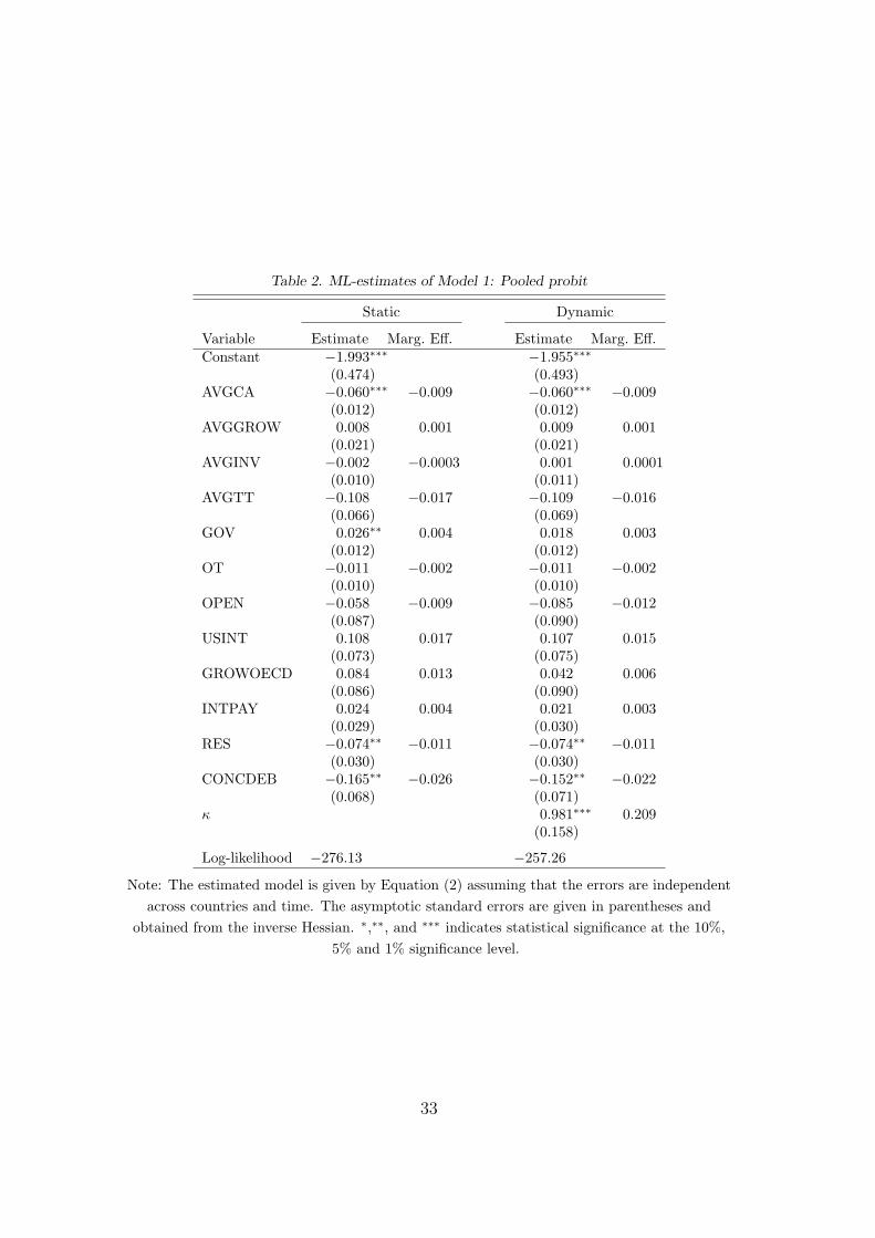
Table 2. ML-estimates of Model 1: Pooled probit
Static Dynamic
Variable Estimate Marg. Eff. Estimate Marg. Eff.Constant −1.993∗∗∗ −1.955∗∗∗
(0.474) (0.493)AVGCA −0.060∗∗∗ −0.009 −0.060∗∗∗ −0.009
(0.012) (0.012)AVGGROW 0.008 0.001 0.009 0.001
(0.021) (0.021)AVGINV −0.002 −0.0003 0.001 0.0001
(0.010) (0.011)AVGTT −0.108 −0.017 −0.109 −0.016
(0.066) (0.069)GOV 0.026∗∗ 0.004 0.018 0.003
(0.012) (0.012)OT −0.011 −0.002 −0.011 −0.002
(0.010) (0.010)OPEN −0.058 −0.009 −0.085 −0.012
(0.087) (0.090)USINT 0.108 0.017 0.107 0.015
(0.073) (0.075)GROWOECD 0.084 0.013 0.042 0.006
(0.086) (0.090)INTPAY 0.024 0.004 0.021 0.003
(0.029) (0.030)RES −0.074∗∗ −0.011 −0.074∗∗ −0.011
(0.030) (0.030)CONCDEB −0.165∗∗ −0.026 −0.152∗∗ −0.022
(0.068) (0.071)κ 0.981∗∗∗ 0.209
(0.158)
Log-likelihood −276.13 −257.26
Note: The estimated model is given by Equation (2) assuming that the errors are independentacross countries and time. The asymptotic standard errors are given in parentheses and
obtained from the inverse Hessian. ∗,∗∗, and ∗∗∗ indicates statistical significance at the 10%,5% and 1% significance level.
33
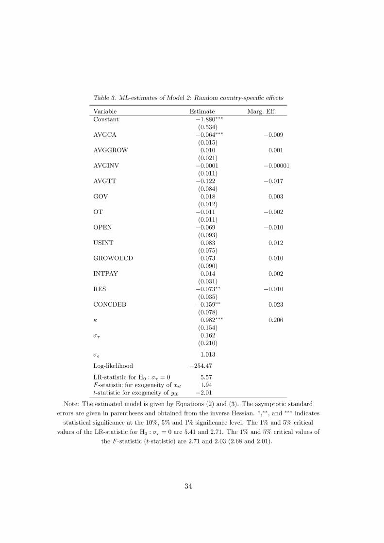
Table 3. ML-estimates of Model 2: Random country-specific effects
Variable Estimate Marg. Eff.Constant −1.880∗∗∗
(0.534)AVGCA −0.064∗∗∗ −0.009
(0.015)AVGGROW 0.010 0.001
(0.021)AVGINV −0.0001 −0.00001
(0.011)AVGTT −0.122 −0.017
(0.084)GOV 0.018 0.003
(0.012)OT −0.011 −0.002
(0.011)OPEN −0.069 −0.010
(0.093)USINT 0.083 0.012
(0.075)GROWOECD 0.073 0.010
(0.090)INTPAY 0.014 0.002
(0.031)RES −0.073∗∗ −0.010
(0.035)CONCDEB −0.159∗∗ −0.023
(0.078)κ 0.982∗∗∗ 0.206
(0.154)στ 0.162
(0.210)
σe 1.013
Log-likelihood −254.47
LR-statistic for H0 : στ = 0 5.57F -statistic for exogeneity of xit 1.94t-statistic for exogeneity of yi0 −2.01
Note: The estimated model is given by Equations (2) and (3). The asymptotic standarderrors are given in parentheses and obtained from the inverse Hessian. ∗,∗∗, and ∗∗∗ indicates
statistical significance at the 10%, 5% and 1% significance level. The 1% and 5% criticalvalues of the LR-statistic for H0 : στ = 0 are 5.41 and 2.71. The 1% and 5% critical values of
the F -statistic (t-statistic) are 2.71 and 2.03 (2.68 and 2.01).
34
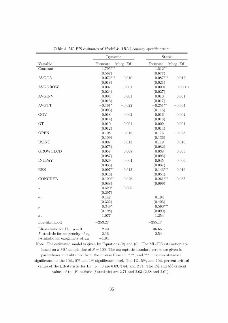
Table 4. ML-EIS estimates of Model 3: AR(1) country-specific errors.
Dynamic Static
Variable Estimate Marg. Eff. Estimate Marg. Eff.Constant −1.795∗∗∗ −1.512∗∗
(0.567) (0.677)AVGCA −0.072∗∗∗ −0.010 −0.087∗∗∗ −0.012
(0.018) (0.021)AVGGROW 0.007 0.001 0.0001 0.00001
(0.024) (0.027)AVGINV 0.004 0.001 0.010 0.001
(0.013) (0.017)AVGTT −0.161∗ −0.022 −0.251∗∗ −0.034
(0.093) (0.116)GOV 0.018 0.002 0.016 0.002
(0.014) (0.018)OT −0.010 −0.001 −0.009 −0.001
(0.012) (0.014)OPEN −0.108 −0.015 −0.175 −0.023
(0.109) (0.136)USINT 0.097 0.013 0.119 0.016
(0.075) (0.082)GROWOECD 0.057 0.008 0.038 0.005
(0.087) (0.095)INTPAY 0.029 0.004 0.045 0.006
(0.035) (0.037)RES −0.097∗∗ −0.013 −0.143∗∗∗ −0.019
(0.046) (0.054)CONCDEB −0.190∗∗ −0.026 −0.261∗∗∗ −0.035
(0.088) (0.099)κ 0.520∗ 0.088
(0.297)στ 0.142 0.194
(0.322) (0.403)ρ 0.349∗ 0.590∗∗∗
(0.198) (0.090)σe 1.077 1.254
Log-likelihood −253.27 −255.17
LR-statistic for H0 : ρ = 0 2.40 36.65F -statistic for exogeneity of xit 2.16 2.54t-statistic for exogeneity of yi0 −1.84
Note: The estimated model is given by Equations (2) and (8). The ML-EIS estimation arebased on a MC sample size of S = 100. The asymptotic standard errors are given inparentheses and obtained from the inverse Hessian. ∗,∗∗, and ∗∗∗ indicates statistical
significance at the 10%, 5% and 1% significance level. The 1%, 5%, and 10% percent criticalvalues of the LR-statistic for H0 : ρ = 0 are 6.63, 3.84, and 2.71. The 1% and 5% critical
values of the F -statistic (t-statistic) are 2.71 and 2.03 (2.68 and 2.01).
35
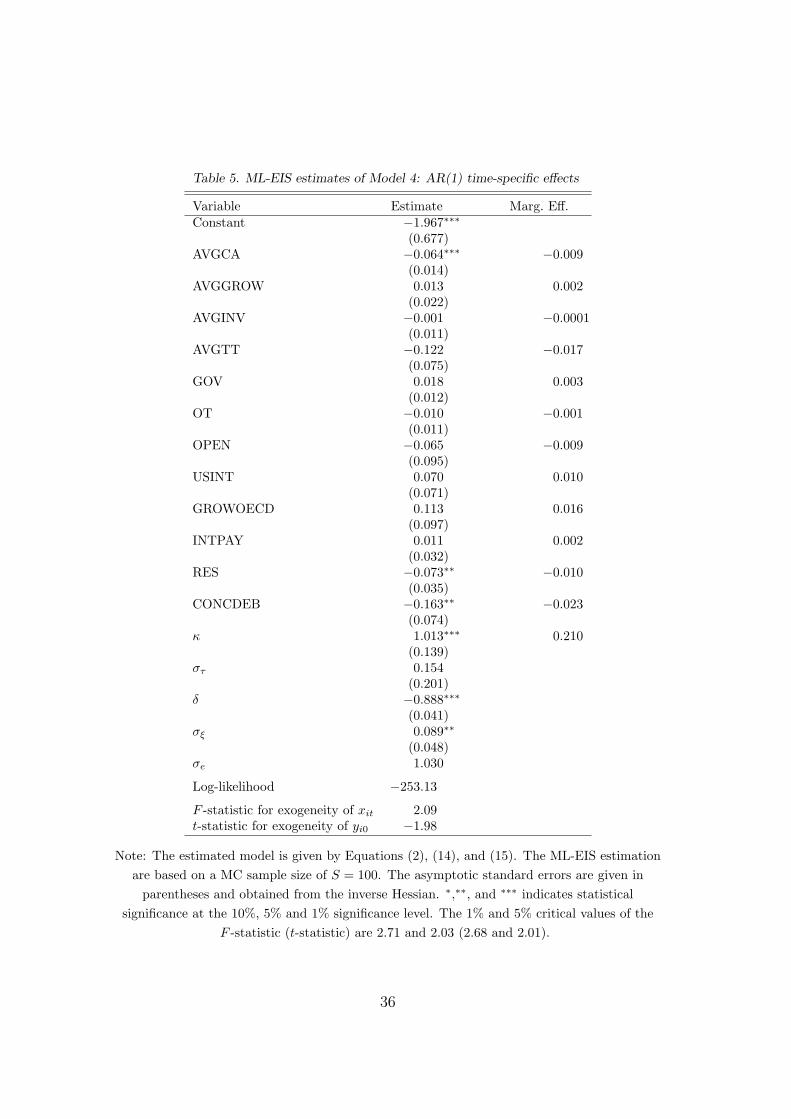
Table 5. ML-EIS estimates of Model 4: AR(1) time-specific effects
Variable Estimate Marg. Eff.Constant −1.967∗∗∗
(0.677)AVGCA −0.064∗∗∗ −0.009
(0.014)AVGGROW 0.013 0.002
(0.022)AVGINV −0.001 −0.0001
(0.011)AVGTT −0.122 −0.017
(0.075)GOV 0.018 0.003
(0.012)OT −0.010 −0.001
(0.011)OPEN −0.065 −0.009
(0.095)USINT 0.070 0.010
(0.071)GROWOECD 0.113 0.016
(0.097)INTPAY 0.011 0.002
(0.032)RES −0.073∗∗ −0.010
(0.035)CONCDEB −0.163∗∗ −0.023
(0.074)κ 1.013∗∗∗ 0.210
(0.139)στ 0.154
(0.201)δ −0.888∗∗∗
(0.041)σξ 0.089∗∗
(0.048)σe 1.030
Log-likelihood −253.13
F -statistic for exogeneity of xit 2.09t-statistic for exogeneity of yi0 −1.98
Note: The estimated model is given by Equations (2), (14), and (15). The ML-EIS estimationare based on a MC sample size of S = 100. The asymptotic standard errors are given in
parentheses and obtained from the inverse Hessian. ∗,∗∗, and ∗∗∗ indicates statisticalsignificance at the 10%, 5% and 1% significance level. The 1% and 5% critical values of the
F -statistic (t-statistic) are 2.71 and 2.03 (2.68 and 2.01).
36

Table 6. Classification errors and predicted average duration in years
ROC averagec∗ α(c∗) β(c∗) area duration
Model 2: Random country-specific 0.11 0.25 0.18 0.85 1.68effects (0.12)
Model 3: AR(1) country-specific 0.12 0.09 0.18 0.91 1.77errors (static) (0.14)
Model 3: AR(1) country-specific 0.09 0.11 0.25 0.88 1.80errors (dynamic) (0.14)
Model 4: AR(1) time-specific 0.08 0.13 0.28 0.86 1.66effects (0.12)
Note: Estimated standard deviation of the predicted average duration are given inparentheses. The observed average duration is 1.52 years.
37
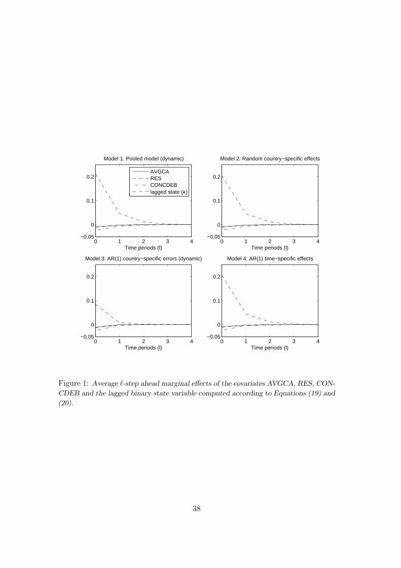
0 1 2 3 4−0.05
0
0.1
0.2
Time periods (l)
Model 1: Pooled model (dynamic)
0 1 2 3 4−0.05
0
0.1
0.2
Time periods (l)
Model 2: Random country−specific effects
0 1 2 3 4−0.05
0
0.1
0.2
Time periods (l)
Model 3: AR(1) country−specific errors (dynamic)
0 1 2 3 4−0.05
0
0.1
0.2
Time periods (l)
Model 4: AR(1) time−specific effects
AVGCARESCONCDEBlagged state (κ)
Figure 1: Average `-step ahead marginal effects of the covariates AVGCA, RES, CON-
CDEB and the lagged binary state variable computed according to Equations (19) and
(20).
38
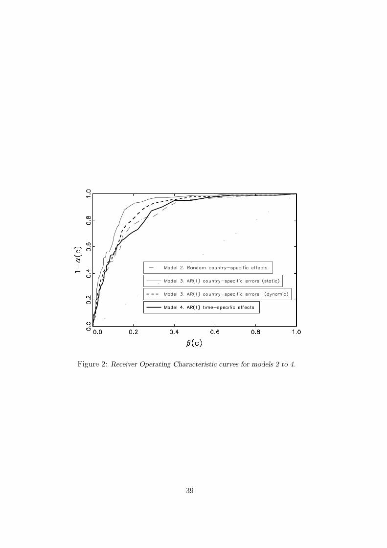
Figure 2: Receiver Operating Characteristic curves for models 2 to 4.
39

Figure 3: Observed and predicted relative frequencies for the duration of reversal
episodes for models 2 to 4. The observed average duration is 1.52 years.
40