


University of Texas at El PasoDigitalCommons@UTEP
Open Access Theses & Dissertations
2011-01-01
Design and CFD Optimization of MethaneRegenerative Cooled Rocket NozzlesChristopher Linn BradfordUniversity of Texas at El Paso, [email protected]
Follow this and additional works at: https://digitalcommons.utep.edu/open_etdPart of the Aerospace Engineering Commons, and the Mechanical Engineering Commons
This is brought to you for free and open access by DigitalCommons@UTEP. It has been accepted for inclusion in Open Access Theses & Dissertationsby an authorized administrator of DigitalCommons@UTEP. For more information, please contact [email protected].
Recommended CitationBradford, Christopher Linn, "Design and CFD Optimization of Methane Regenerative Cooled Rocket Nozzles" (2011). Open AccessTheses & Dissertations. 2242.https://digitalcommons.utep.edu/open_etd/2242

DESIGN AND CFD OPTIMIZATION OF METHANE
REGENERATIVE COOLED ROCKET NOZZLES
CHRISTOPHER LINN BRADFORD
Department of Mechanical Engineering
APPROVED :
__________________________________ Jack Chessa, Ph.D., Chair
__________________________________ Ahsan Choudhuri, Ph.D.
__________________________________ Cesar Carrasco, Ph.D.
__________________________________ Benjamin C. Flores, Ph.D. Acting Dean of the Graduate School

Copyright ©
By
Christopher Linn Bradford
2011

DESIGN AND CFD OPTIMIZATION OF METHANE
REGENERATIVE COOLED ROCKET NOZZLES
by
CHRISTOPHER LINN BRADFORD, B.S.A.E.
THESIS
Presented to the Faculty of the Graduate School of
The University of Texas at El Paso
in Partial Fulfillment
of the Requirements
for the Degree of
MASTER OF SCIENCE
Department of Mechanical Engineering
THE UNIVERSITY OF TEXAS AT EL PASO
August 2011

iv
ACKNOWLEDGEMENTS
The material contained herein is being conducted in conjunction with work for the Center for
Space Exploration Technology Research (cSETR) at the University of Texas at El Paso, under
principal investigator Dr. Ahsan Choudhuri. The cSETR is a National Aeronautics and Space
Administration (NASA) supported Group 5 University Research Center awarded in fiscal year
2009 under award number NNX09AV09A. More information can be found at [1] and [2].

v
TABLE OF CONTENTS
Page
ACKNOWLEDGEMENTS ........................................................................................................... iv
LIST OF TABLES ......................................................................................................................... ix
LIST OF FIGURES ...................................................................................................................... xii
1 INTRODUCTION TO THE REGENERATIVE COOLING CONCEPT................................. 1
2 LITERATURE REVIEW CONCERNING REGENERATIVE COOLING ............................. 9
2.1 Cooling System Construction and Geometric Considerations.................................... 9
2.2 Standard Materials Used in Engine Construction ..................................................... 19
2.3 Cooling Channel Pressure Requirements .................................................................. 26
2.4 Aspects of Heat Transfer .......................................................................................... 29
2.4.1 Basic Heat Transfer Theory ........................................................................... 29
2.4.2 Gas Side Heat Transfer .................................................................................. 30
2.4.3 Regenerative Cooling and Coolant Side Heat Transfer ................................. 34
2.4.4 Solid to Solid Heat Transfer .......................................................................... 36
2.4.5 Outer Shell Heat Transfer .............................................................................. 37
2.5 Material Loading, Stress, and Failure ....................................................................... 37
2.6 Using Methane as the Coolant and Fuel ................................................................... 42
2.7 Computational Modeling and CFD ........................................................................... 47
2.8 Ideal Versus Real Gas Modeling .............................................................................. 56
2.9 The cSETR 50lbf Thrust Engine ............................................................................... 58
3 MATHEMATICAL THEORY OF REGENERATIVE COOLING ....................................... 60
3.1 Cooling Channel Pressure Relationships .................................................................. 60

vi
3.2 Theory of Cooling System Heat Transfer ................................................................. 61
3.2.1 Basic Heat Transfer Theory ........................................................................... 62
3.2.2 Gas Side Heat Transfer .................................................................................. 65
3.2.3 Coolant Side, and Solid to Solid, Heat Transfer ........................................... 69
3.2.4 Outer Shell Heat Transfer .............................................................................. 74
3.3 Theory of Material Loading, Stress, and Failure ...................................................... 75
3.3.1 Cylindrical Pressure Vessel Analogy............................................................. 75
3.3.2 Fixed End Beam With Uniform Pressure Load Analogy .............................. 76
3.3.3 Fixed End Beam With Uniform Temperature Load Analogy ....................... 79
3.3.4 Column Subject To Buckling Analogy .......................................................... 80
3.3.5 Recommended Criteria For Loads ................................................................. 82
3.3.6 Simplified Theory of Cyclic Loading Stress Analysis .................................. 83
3.4 Using Methane as the Coolant and Fuel ................................................................... 84
3.5 Theory Required for Computational Modeling and CFD ......................................... 87
3.5.1 Mesh Considerations, "y" Values, Etc. .......................................................... 87
3.5.2 Turbulence Model Parameters ....................................................................... 91
3.5.3 Pre-Channel Entrance Length ........................................................................ 94
4 METHODOLOGY TO DESIGN AND OPTIMIZE REGENERATIVE COOLING CHANNELS ......................................................................................................... 96
4.1 Preliminary Stress Analysis ...................................................................................... 96
4.1.1 Analysis of Loading Conditions .................................................................... 96
4.1.2 Chamber Wall Thickness Determination ....................................................... 99
4.1.3 Outer Shell Thickness Determination .......................................................... 102
4.1.4 Channel Width to Chamber Wall Thickness Design Ratio ......................... 102
4.1.5 Fin Width to Channel Width Design Ratio .................................................. 106

vii
4.1.6 Fin Height to Fin Width Design Ratio ......................................................... 107
4.1.7 Summary of Important Values for Later Use .............................................. 108
4.2 Thermal Analysis .................................................................................................... 109
4.2.1 Combustion Chamber Thermal Conditions ................................................. 109
4.2.1.1 adiabatic flame temperature of combustion .................................... 110
4.2.1.2 parameters needed for the Bartz equation ....................................... 112
4.2.1.3 Bartz heat transfer coefficient variation .......................................... 114
4.2.2 Fin and Cooling Channel Thermal Conditions ............................................ 115
4.2.2.1 fin height and heat transfer coefficients .......................................... 115
4.2.2.2 parameters needed for coolant side heat transfer ............................ 117
4.2.2.3 iteration of fin height equation ........................................................ 118
4.2.3 Outer Shell Thermal Conditions .................................................................. 121
4.3 Pre-Channel Flow Calculations .............................................................................. 122
4.4 CFD Setup Parameters ............................................................................................ 122
4.4.1 Geometry Organization ................................................................................ 122
4.4.2 Initial Mesh Determination .......................................................................... 123
4.4.3 HyperMesh Geometry Generation ............................................................... 124
4.4.4 FLUENT Setup Parameters ......................................................................... 128
4.4.4.1 boundary condition input files ........................................................ 128
4.4.4.2 turbulence model parameters .......................................................... 128
4.4.4.3 FLUENT case options and parameters ........................................... 129
4.5 Running the CFD Simulations ................................................................................ 133
4.5.1 General Simulation Running Techniques and Behavior .............................. 133
4.5.2 Mesh & Turbulence Sensitivity Study ......................................................... 134
4.5.3 Main Study ................................................................................................... 135
viii
5 RESULTS OF THE MAIN STUDY CFD OPTIMIZATION SIMULATIONS ................... 137
5.1 General Performance Characteristics ...................................................................... 137
5.2 Performance Considering nc ................................................................................... 144
5.3 Performance Considering Geometry Features ........................................................ 154
5.4 Relating Ideal and Real Gas Behavior .................................................................... 164
6 CONCLUSIONS.................................................................................................................... 168
7 RECOMMENTATIONS FOR FUTURE RESEARCHERS ................................................. 171
REFERENCES ........................................................................................................................... 173
APPENDIX I: MAPLE Code to Calculate Adiabatic Flame Temperature ............................... 178
APPENDIX II: Bartz Heat Transfer Coefficient Values Along True Length ........................... 181
APPENDIX III: MATLAB Code to Iterate the Fin Height Equation ....................................... 185
APPENDIX IV: Results of Fin Height Iteration........................................................................ 190
APPENDIX V: Drawing Coordinates for CFD geometry ......................................................... 193
CURRICULUM VITA ............................................................................................................... 197
ix
LIST OF TABLES
Page
Table 2-1: Geometric values for channels tested in [16]. ............................................................ 14
Table 2-2: Geometric values for channels tested in [18]. ............................................................ 15
Table 2-3: Select geometric values for channels which consider fabrication from [6]. Note: values are not for the same axial location. ................................................. 16
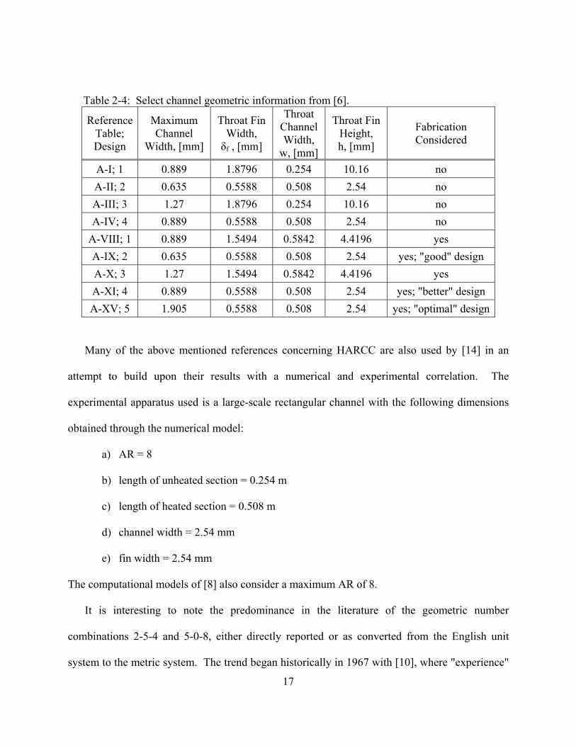
Table 2-4: Select channel geometric information from [6]. ........................................................ 17
Table 2-5: Useful NARloy-Z material property data at the elevated temperatures expected, from various sources. ............................................................................................ 25
Table 2-6: Useful Copper material property data at the elevated temperatures expected, from various sources. ............................................................................................ 26
Table 2-7: Useful Inconel 718 material property data at the elevated temperatures expected, from [24]. .............................................................................................. 26
Table 2-8: Structural results for channels tested in [18]. ............................................................. 40
Table 2-9: Pressure and temperature conditions of methane found from the analysis of [7]. ..... 45
Table 2-10: Pressure and temperature conditions of methane used by [8]. ................................. 45
Table 2-11: Various point property values for methane. ............................................................. 46
Table 2-12: Useful heats (enthalpies) of formation at 298.15 K from [28], and compound molar masses (molecular weights) from [40]. ...................................................... 47
Table 2-13: Preferred smooth wall y+ ranges of various references. ........................................... 49
Table 2-14: Suggestions for turbulence intensity factor of various references. .......................... 50
Table 2-15: FLUENT turbulence model default constants and suggestions, per [47], [48], [51]. Note: values include standard wall functions and viscous heating. ........... 54
Table 2-16: FLUENT default solution control, under-, and explicit- relaxation factors, per [47], [48], and [51]. ............................................................................................... 55

x
Table 2-17: Useful FLUENT Material Property Database values, from the software interface and through [48] referenced files. .......................................................... 55
Table 2-18: Various cSETR 50lbf thrust engine geometric and operating parameters, from [9] and using Figure 1-10. ..................................................................................... 59
Table 3-1: Ideal gas specific heats of expected combustion reactants and products, from [28]. ....................................................................................................................... 86
Table 4-1: Yield and ultimate load conditions for the inner and outer shells. ............................. 98
Table 4-2: Various calculated chamber wall thicknesses for minimal safety factor yield criteria designs. Equation (31) used with listed input parameters, rcc = 0.01625 m, and pc = 1.5 x 10⁶ N/m2. .................................................................. 100
Table 4-3: Various calculated chamber wall thicknesses for working loads yield criteria designs. Equation (31) used with listed input parameters, rcc = 0.01625 m, and LY inner = 2.02125 x 10⁶ N/m2. ....................................................................... 100
Table 4-4: Various calculated chamber wall thicknesses for working loads ultimate or endurance criteria designs. Equation (31) used with listed input parameters, rcc = 0.01625 m, and LU inner = 2.75625 x 10⁶ N/m2. ........................................... 101
Table 4-5: Various calculated outer shell thicknesses for Inconel 718 subject to different loading conditions. Equation (31) used with listed input parameters and rJ = 25.065 mm. ......................................................................................................... 102
Table 4-6: Literature values of the channel width to chamber wall thickness ratio, as found from [16] and Table 2-1. ..................................................................................... 103
Table 4-7: Literature values of the channel width to chamber wall thickness ratio, as found from [6] and Table 2-4. ....................................................................................... 104
Table 4-8: Literature values of the channel width to chamber wall thickness ratio, as found from [18] and Table 2-2. ..................................................................................... 104
Table 4-9: Values of the channel width to chamber wall thickness ratio for various inner shell materials, as found from Equation (55). ..................................................... 105
Table 4-10: Literature values of the fin width to channel width ratio, as found from [12] and Table 2-4. ..................................................................................................... 106
Table 4-11: Literature values of the fin height to fin width ratio, as found from Table 2-4. .... 107
Table 4-12: Summary of important values to be used in the present research for subsequent calculations and comparison. ........................................................... 108

xi
Table 4-13: FLUENT models prescribed. ................................................................................. 129
Table 4-14: FLUENT viscosity model parameters prescribed. ................................................. 130
Table 4-15: FLUENT domain values prescribed. ...................................................................... 130
Table 4-16: Bottom-wall-bottom (hot-wall) FLUENT wall zone boundary conditions. ........... 131
Table 4-17: Inlet FLUENT mass flow inlet zone boundary conditions. .................................... 131
Table 4-18: Outlet FLUENT pressure outlet zone boundary conditions. .................................. 131
Table 4-19: Top-wall-top FLUENT wall zone boundary conditions. ....................................... 131
Table 4-20: Various other FLUENT boundary conditions. ....................................................... 132
Table 4-21: FLUENT solution monitors, methods and controls. .............................................. 132
Table 4-22: Mesh & turbulence sensitivity study fluid domain mesh densities. ....................... 134
Table 5-1: Numerical comparison between nc = 29 results using ideal and real gas. ................ 167
Table 6-1: Summary of the parameters for the concluded optimal cooling channel configuration on the cSETR 50lbf engine, using ideal gas methane as the coolant. Values reported are for static ground test conditions (convection outer shell CFD boundary condition). ................................................................ 169
Table 6-2: Numerical comparison between nc = 29 results and the results of the same configuration with a reduced mass flow rate. ..................................................... 170

xii
LIST OF FIGURES
Page
Figure 1-1: Conceptual view of the regenerative cooling technique for a bi-propellant liquid rocket engine. Obtained from [3]. ............................................................... 2
Figure 1-2: Typical milled out liquid rocket engine cooling channel application on the inner liner with detached outer jacket portion. Obtained from [4]. ....................... 2
Figure 1-3: Typical cross section showing copper alloy inner liner with milled out channels and applied nickel alloy outer jacket. Obtained from [4]. ...................... 2
Figure 1-4: Conceptual view of engine cross section portion showing details of construction. Obtained from [3]. ............................................................................ 3
Figure 1-5: Example of possible channel cross sectional size, shape, and topology designs. Obtained from [5]. .................................................................................................. 3
Figure 1-6: Rectangular channel with aspect ratio defined. Tgw represents the temperature of the wall inside the combustion chamber. Obtained from [6]. ....... 3
Figure 1-7: Various channel lengthwise shapes as viewed from the top. Obtained from [6]. ........................................................................................................................... 3
Figure 1-8: Cyclic thinning damage and failure due to material fatigue at the bottom of the channel. Adapted from [5]. .................................................................................... 5
Figure 1-9: Typical hydrogen and methane channel operational conditions, with reduced constant pressure specific heat contours. Obtained from [8]. ................................ 6
Figure 1-10: cSETR designed 50lbf thrust rocket engine, units of "mm [in]". Obtained from [9]. .................................................................................................................. 8
Figure 2-1: Rupture life of NARloy-Z at elevated temperatures. Obtained from [15]. .............. 21
Figure 2-2: Stress-strain curves for NARloy-Z at various temperatures. Obtained from [25]. ....................................................................................................................... 22
Figure 2-3: Cyclic stress-strain curve for NARloy-Z at 810.9 K. Obtained from [25]. ............. 23
Figure 2-4: Stress-strain curves for OFHC Copper Annealed at various temperatures. Obtained from [25]. .............................................................................................. 24

xiii
Figure 2-5: Bartz equation correction factor values (σ) for various temperature and specific heat (γ) ratios at axial locations of ξ. ξ is the ratio of the local area to the throat area. ξC is in the chamber, one indicates the throat, ξ is in the nozzle. Obtained from [10]. ................................................................................. 32
Figure 2-6: 1D heat transfer schematic representation of regenerative cooling. Obtained from [10]. .............................................................................................................. 35
Figure 2-7: Allowable cooling channel pressure drop for O2/CH4 systems as a function of chamber pressure. Obtained from [16]. ............................................................... 44
Figure 3-1: Linear interpolation terms of Equation (13). ............................................................ 67
Figure 3-2: Statically indeterminate fixed-end beam representation of chamber wall span between two fins, at the bottom of one cooling channel. ...................................... 76
Figure 3-3: Illustration of effective pressure acting on the chamber wall. .................................. 77
Figure 3-4: Beam representation as seen along the y axis. .......................................................... 78
Figure 3-5: Cooling fin represented as a column subjected to buckling loads. ........................... 80
Figure 3-6: Column representation as seen along the z axis. ....................................................... 81
Figure 3-7: Distance of the near-wall computational node to the solid surface for a 3D CFD element. ........................................................................................................ 89
Figure 4-1: Heat transfer coefficient variation of Bartz along the cSETR 50lbf engine hot-wall versus length along hot-wall. The left portion is in the engine nozzle, the peak indicates the throat, and the right portion is in the combustion chamber. Values correspond to Appendix II. .................................................... 114
Figure 4-2: Geometry variation for the channel models nc of channel height. Values correspond to Appendix IV. ................................................................................ 119
Figure 4-3: Geometry variation for the channel models nc of the CFD modeled channel half widths. Values correspond to Appendix IV. ............................................... 120
Figure 4-4: Geometry variation for the channel models nc of the channel aspect ratio using the channel height and full width. Values correspond to Appendix IV. ............ 120
Figure 4-5: Flow variation for the channel models nc of the channel mass flow rate. Values correspond to Appendix IV. .................................................................... 121
Figure 4-6: Representation of the CFD modeled geometry with drawing coordinate locations indicated. Points associated with Appendix V. .................................. 123

xiv
Figure 4-7: 2D wall zones, channel inlets and outlet, and 3D regions. ..................................... 125
Figure 4-8: Isometric view of entire representative channel. .................................................... 125
Figure 4-9: Modeled-inlet area showing the solid domains for a representative channel. ........ 126
Figure 4-10: Alternate view of modeled-inlet area for a representative channel. ..................... 126
Figure 4-11: View of inlet of a representative channel showing solid domains, mesh, and half channel and fin widths. Symmetry planes are on both the left and right sides..................................................................................................................... 127
Figure 4-12: Main study initialized x velocity variation for the channel models nc for both convection and radiation boundary types. .......................................................... 136
Figure 4-13: Main study initialized temperature variation for the channel models nc for both convection and radiation boundary types. .................................................. 136
Figure 5-1: Overview of the temperature variation in the solid domains of a representative channel at the heated section............................................................................... 139
Figure 5-2: Overview of the heat flux variation on the bottom-wall-bottom (lower) and top-wall-top (upper) of a representative channel at the heated section. ............. 140
Figure 5-3: Overview of the density variation in the fluid domain of a representative channel at the heated section. The dark blue areas are the constant density solid domains. ..................................................................................................... 141
Figure 5-4: Variation of fluid density at multiple lengthwise locations along the heated section of a representative channel, between the modeled inlet and the outlet, with adjacent solid values. ....................................................................... 142
Figure 5-5: Variation of fluid temperature at multiple lengthwise locations along the heated section of a representative channel, between the modeled inlet and outlet, with adjacent solid values. ....................................................................... 143
Figure 5-6: Maximum wall temperatures on the bottom-wall-bottom (hot-wall) 2D wall zone for channel models nc. ................................................................................ 145
Figure 5-7: Maximum wall heat flux values on the bottom-wall-bottom (hot-wall) 2D wall zone for channel models nc. ................................................................................ 145
Figure 5-8: Maximum wall temperatures on the channel-bottom 2D wall zone for channel models nc. ............................................................................................................ 146

xv
Figure 5-9: Maximum wall temperatures on the channel-left 2D wall zone for channel models nc. ............................................................................................................ 146
Figure 5-10: Maximum wall temperatures on the top-wall-top 2D wall zone for channel models nc. ............................................................................................................ 147
Figure 5-11: Channel pressure drops between the modeled-inlet and the outlet for channel models nc. ............................................................................................................ 147
Figure 5-12: First derivatives of the channel pressure drops between the modeled-inlet and the outlet for channel models nc. ......................................................................... 148
Figure 5-13: Second derivatives of the channel pressure drops between the modeled-inlet and the outlet for channel models nc. .................................................................. 148
Figure 5-14: Channel velocity increases between the modeled-inlet and the outlet for channel models nc. .............................................................................................. 149
Figure 5-15: First derivatives of the channel velocity increases between the modeled-inlet and the outlet for channel models nc. .................................................................. 149
Figure 5-16: Second derivatives of the channel velocity increases between the modeled-inlet and the outlet for channel models nc. .......................................................... 150
Figure 5-17: Channel coolant temperature increases between the modeled-inlet and the outlet for channel models nc. ............................................................................... 150
Figure 5-18: First derivatives of the channel temperature increases between the modeled-inlet and the outlet for channel models nc. .......................................................... 151
Figure 5-19: Second derivatives of the channel temperature increases between the modeled-inlet and the outlet for channel models nc. ........................................... 151
Figure 5-20: Net heat flux quantities entering the channel through the surrounding 2D walls for channel models nc. ............................................................................... 152
Figure 5-21: First derivative of the net heat flux quantities entering the channel through the surrounding 2D walls for channel models nc. ............................................... 152
Figure 5-22: Second derivative of the net heat flux quantities entering the channel through the surrounding 2D walls for channel models nc. ............................................... 153
Figure 5-23: Channel hydraulic diameters for the range of aspect ratios considered. ............... 155
Figure 5-24: Maximum wall temperature on the bottom-wall-bottom (hot-wall) 2D wall zone for the range of aspect ratios considered. ................................................... 155

xvi
Figure 5-25: Maximum wall temperature on the bottom-wall-bottom (hot-wall) 2D wall zone for the range of hydraulic diameters considered. ....................................... 156
Figure 5-26: Maximum wall heat flux on the bottom-wall-bottom (hot-wall) 2D wall zone for the range of aspect ratios considered.. ........................................................... 156
Figure 5-27: Maximum wall heat flux on the bottom-wall-bottom (hot-wall) 2D wall zone for the range of hydraulic diameters considered. ................................................ 157
Figure 5-28: Maximum wall temperature on the channel-bottom 2D wall zone for the range of aspect ratios considered.. ...................................................................... 157
Figure 5-29: Maximum wall temperature on the channel-bottom 2D wall zone for the range of hydraulic diameters considered. ........................................................... 158
Figure 5-30: Maximum wall temperature on the channel-left 2D wall zone for the range of aspect ratios considered.. .................................................................................... 158
Figure 5-31: Maximum wall temperature on the channel-left 2D wall zone for the range of hydraulic diameters considered........................................................................... 159
Figure 5-32: Maximum wall temperature on the top-wall-top 2D wall zone for the range of aspect ratios considered. ..................................................................................... 159
Figure 5-33: Maximum wall temperature on the top-wall-top 2D wall zone for the range of hydraulic diameters considered........................................................................... 160
Figure 5-34: Channel pressure drop between the modeled-inlet and the outlet for the range of aspect ratios considered. ................................................................................. 160
Figure 5-35: Channel pressure drop between the modeled-inlet and the outlet for the range of hydraulic diameters considered. ..................................................................... 161
Figure 5-36: Channel velocity increase between the modeled-inlet and the outlet for the range of aspect ratios considered. ....................................................................... 161
Figure 5-37: Channel velocity increase between the modeled-inlet and the outlet for the range of hydraulic diameters considered. ........................................................... 162
Figure 5-38: Channel temperature increase between the modeled-inlet and the outlet for the range of aspect ratios considered. ................................................................. 162
Figure 5-39: Channel temperature increase between the modeled-inlet and the outlet for the range of hydraulic diameters considered. ..................................................... 163

xvii
Figure 5-40: Net heat flux quantities entering the channel through the surrounding 2D walls for the range of aspect ratios considered. .................................................. 163
Figure 5-41: Net heat flux quantities entering the channel through the surrounding 2D walls for the range of hydraulic diameters considered. ...................................... 164
Figure 5-42: Ideal gas (red) and real gas (blue) CFD rake results superimposed upon the real gas methane state diagram considered by [55]. Adapted from [55]. .......... 165
Figure 5-43: Ideal gas (red) and real gas (blue) CFD rake results showing density variation and gas model discrepancies. .............................................................................. 167

1
CHAPTER 1
INTRODUCTION TO THE REGENERATIVE COOLING CONCEPT
The extreme thermal and stress loadings encountered by rocket engine combustion chambers
is of critical importance to the design life of the engine, and subsequently the mission life of the
unit to which the engine is attached. Missions beyond the orbit of Earth into deep space require
a highly reliable engine with a long life of multiple firing cycles, especially since the engine is
not able to be serviced once launched. Adequate cooling of the engine nozzle, throat, and
combustion chamber is essential for such long equipment lives, and is typically performed
through some active cooling method.
The use of regenerative cooling involves the fuel of a liquid fed engine being forced through
channels adjacent to or forming the nozzle, throat, and chamber walls. A conceptual view of the
process is shown in Figure 1-1. Typical applications are shown in Figures 1-2 and 1-3, where
the channels are milled out of an inner liner wall (usually some copper alloy) and closed off by
an applied outer jacket shell (usually some nickel alloy), which is marked conceptually in Figure
1-4. There are many machinable cross sectional sizes, shapes, and topologies possible for the
channels as can be seen in Figure 1-5. In particular, the size is determined by the aspect ratio
(AR) of the cross section for the rectangular shape, seen and defined in Figure 1-6. Changing the
cross section along the channel length is also a possibility, and is especially important in the
design for optimal channel pressure drop from the inlet to the outlet. Various lengthwise shapes
are shown in Figure 1-7. Finally, the number of channels placed about the engine circumference
can be varied, all for the purpose of optimal heat transfer away from the wall and to the cooling
fluid with an acceptable pressure drop along the channel length.

2
Figure 1-1: Conceptual view of the regenerative cooling technique for a bi-propellant liquid rocket engine. Obtained from [3].
Figure 1-2: Typical milled out liquid rocket engine cooling channel application on the inner liner with detached outer jacket portion. Obtained from [4].
Figure 1-3: Typical cross section showing copper alloy inner liner with milled out channels and applied nickel alloy outer jacket. Obtained from [4].

3
Figure 1-4: Conceptual view of engine cross section portion showing details of construction. Obtained from [3].
Figure 1-5: Example of possible channel cross sectional size, shape, and topology designs. Obtained from [5].
Figure 1-6: Rectangular channel with aspect ratio defined. Tgw represents the temperature of the wall inside the combustion chamber. Obtained from [6].
Figure 1-7: Various channel lengthwise shapes as viewed from the top. Obtained from [6].

4
During the steady state cooling process, the relatively lower temperature fuel picks up the
heat conducted into the walls, and reduces the wall temperature to below critical material failure
levels. As the walls are cooled the fuel is warmed, and depending on the feed system design of
the particular engine, is either used to drive fuel and oxidizer pumps in an expander cycle and
then sent to the injector plate, or directly dumped into the injector plate before entering the
combustion chamber.
In most liquid rocket engines the non-steady state transient processes of throttling and
pulsing the thrust, and stopping and restarting the engine are experienced. The changes in
pressure and temperature then become higher over a shorter amount of time, and introduce the
problems of cyclic loading, thinning, and failure due to material fatigue. Because of the inherent
design of regenerative cooling, the location of highest fatigue stress and weakest structural
strength can be at the bottoms of the cooling passages. This location separates the combustion
gasses from the coolant, so material failure in this location would lead to total engine failure.
Figure 1-8 depicts this scenario as well as indicates the locations of the other structural members
in the vicinity where failure can occur, i.e. the fins and jacket.
The design of the cooling passages for adequate structural integrity is directly dependent
upon the materials used and the cross sectional geometry details. A preliminary stress analysis
must be performed even if the cooling performance is the primary focus. Then upon completion
of the initial cooling passage design, a more detailed stress analysis would be necessary and
structural improvements made. The structural improvements will affect the cooling
performance, and the second cooling passage design iteration would be necessary, et cetera until
the engine design is both structurally and thermally optimal. Furthermore, the design of the
cooling passages for optimal cooling performance is highly dependent upon the fuel used in the

5
engine because of the different properties and behaviors of various useful propellants.
Figure 1-8: Cyclic thinning damage and failure due to material fatigue at the bottom of the channel. Adapted from [5].
The use of methane is attractive as the fuel for deep space missions because of its abundance
on terrestrial bodies encountered in the exploration path. This abundance also opens the
possibility for reduced initial launch weights from Earth, as the full-capacity fuel supply is not
required at the launch time. Through a process known as "in-situ resource utilization", the fuel
supply can be gained or refurbished during the mission, as mentioned in [7]. A liquid propellant
engine designed to the properties of methane as the fuel are thus required. As shown in Figure
1-9 however, the typical operating conditions for methane are much closer to the critical point
where phase change is a likely possibility, in contrast to the conditions of a more typical fuel
such as hydrogen. The likelihood of phase change adds to the difficulty in modeling and using
methane.

6
Figure 1-9: Typical hydrogen and methane channel operational conditions, with reduced constant pressure specific heat contours. Obtained from [8].
Various modeling options are available to represent the behavior of fluid materials. The use
of computational methods not only reduces the time and expense required in a design, but also
allows for multiple design iterations to be performed before a finalized "best" design is
determined. Luckily computational fluid dynamics (CFD) software is available with the desired
features, but challenges remain. As with any commercially available modeling software, or
software that the user does not create themselves, it is essential to research the software
functionality and limitations in detail before attempting to model any process with the desire to
achieve useful results.
The objective of the present research is to design the regenerative cooling channels for the
current 50 pound force (lbf) thrust engine designed and studied by the Center for Space

7
Exploration Technology Research (cSETR), per [9]. The engine design as shown in Figure 1-10
has the purpose of using methane as the fuel and coolant, with liquid oxygen as the oxidizer.
Methane is thus used as the working fluid for the channels in the present research. A
comprehensive literature review is performed to account for the limited sources of directly
applicable design information relevant to the specifics of using methane as the fuel for this thrust
class of engine. Taking only the inner shape of the engine, a preliminary stress analysis is
performed to obtain certain material geometric features. A preliminary thermal and flow
analysis is then performed to obtain additional geometric and flow details. These features are
then built into computational models to obtain a baseline design set. The CFD software ANSYS
FLUENT, version 12.1.4, is next used to determine the optimal configuration for the first
iteration of the channel design, and an analysis of the results given. Finally, improvements and
suggestions for future researchers are given.

8
Figure 1-10: cSETR designed 50lbf thrust rocket engine, units of "mm [in]". Obtained from [9].

9
CHAPTER 2
LITERATURE REVIEW CONCERNING REGENERATIVE COOLING
In this chapter, a review of past work in the field of regenerative cooling of liquid rocket
engines and the use of methane as both the coolant and the fuel is presented. The importance of
an integrated engine cooling system (rather than an added-on feature) necessitates the
consideration of multiple engine design aspects. General information obtained from the
references is given, with specific mathematical equations placed in the subsequent chapter on
mathematical theory. Units have been converted to usable values.
2.1 Cooling System Construction and Geometric Considerations
The construction of liquid propellant rocket engines with the purpose of utilizing
regenerative cooling can be carried out using two main methods, both depending on the
application. The choice of method depends on many factors.
The first method is tubular wall thrust chamber design, detailed in [10], and involves forming
the combustion chamber and nozzle using individual tubes which are joined together and held in
place with outer rings. The tubes carry the fuel to act as the coolant. Experience and assumption
are used for some sample calculations of [10] to state that the tube wall thicknesses for one
hypothetical case study design using the Inconel X material is sufficient for the throat at 0.508
millimeters (mm). A value of 0.2032 mm is also given "from experience" for a separate sample
calculation.
The second construction method, coaxial shell thrust chamber design, is only briefly
described in [10]. This method involves the combustion chamber, throat, and nozzle created out

10
of one piece of metal, forming the inner shell. Other terms used in literature for the inner shell
are: "inner liner", "combustion chamber liner", "inner wall", or similar. Material is either cut or
otherwise extracted from the inner shell material to leave the cooling channel voids; also known
as the "slots". The voids are enclosed by an additional outer piece called the outer shell. Other
terms for the outer shell are: "outer wall", "outer jacket", "external jacket", "liner closeout",
"closeout", "ligament", or similar. This coaxial shell method is seen in Figures 1-2, 1-3, and 1-4.
As explained in [11], this channel construction method has become the preferred for regions of
the engine requiring critical cooling capability. The size of the cSETR 50lbf engine of Figure
1-10 indicates that coaxial shell construction is the best method.
When the channels are created in the inner shell, the cross sectional distance between the
bottom of the channels and the opposite surface adjacent to the hot combustion chamber gasses
becomes the thinnest portion, termed the chamber wall. This is a critical design thickness
deserving special attention. Other terms found in literature are: "liner", "inner shell thickness",
"combustion chamber wall", "inner wall", "chamber inner wall" (sometimes a term for the
combustion chamber wall surface adjacent to the hot gasses), "wall thickness", or similar.
The remaining material adjacent to the channel voids also becomes a critical design
component for structural and thermal considerations, termed the fins. Other terms found in
literature are: "web", "side wall", "channel side wall", "land", "landwidth", "fin width", "fin
thickness", "rib", or similar. Furthermore, the terms "fin height", "channel height", "depth", or
"channel depth" are equivalent.
Additional detail can be built into the channel geometry as important features affecting the
cooling system performance. For tubular construction, [10] shows that the tubes can either be
circular in cross section, elongated, or vary from circular to nearly square elongated as the

11
channel progresses along the axial length of the engine. One purpose for the cross sectional area
variation is to adjust the coolant velocity as required for adequate heat transfer at any particular
location, which has implications for the local and overall channel coolant pressure. Avoiding
sudden changes in the flow direction or cross sectional area was mentioned. The coaxial shell
construction used in [6] allows the channel geometries seen in Figure 1-7 with the same effect.
At the entrance of the channels, [11] shows that a circumferential manifold is required to
inject the coolant and distribute it evenly to all channels, requiring flow direction and area
changes. At the exit, a coolant-return manifold is required to capture the coolant for placement
into the mixing head and injector plate. The cooling channel design can be performed without
considering the manifold heat transfer effects, but should consider some flow effects.
The "Thermal SkinTM" fabrication concept of [12] is similar to the coaxial shell design when
seen in cross section. For a rectangular shape, the "based on past experience" and 1968 state-of-
the-art channel fabrication limits are given as:
a) maximum AR = 1.33
b) minimum channel width possible, w = 0.3048 mm
c) minimum fin width possible, δf = 0.381 mm
d) minimum chamber wall thickness possible, t = 0.635 mm
e) fin width to channel width ratio, (δf /w) = 1
An unexplained analysis is referenced to suggest that these dimensions maximize the fin
efficiency. The efficiency concept is found in [6] and [13], and used with more detail in [7] and
[14].
The modern Space Shuttle Main Engine (SSME) also utilizes the coaxial shell construction
method, but as explained in [15] there are three shells: inner, middle, and outer. A comparison

12
to tubular construction is made, showing that for temperature considerations the coaxial shell
channels are preferred over tubes. From a pressure stress consideration, a thinner wall is
achievable using tubes with the manufacturing limits of the time for channels. The discussion of
channel geometry suggests that the SSME channels are manufactured using the 1973 state-of-
the-art milling fabrication limits. For a rectangular cross section, the SSME channel geometry is
given as:
a) channel width, w = 1.016 mm
b) channel height, h = 2.54 mm
c) closeout (middle shell layer) thickness, tm = ~1.27 mm
d) unspecified chamber wall thickness; range analyzed = 0.508 mm to 0.7112 mm
The effect of combustion chamber wall thickness in relation to the maximum thermal benefit is
discussed and shown in a figure with some ambiguity. The construction at the throat region of
the SSME is detailed in [11] and shows that the throat can be considered comprised of only the
inner and middle shells. Channel geometry is given there as:
a) throat channel width, w = 1.016 mm
b) throat chamber wall thickness, t = 0.7112 mm
c) non-throat channel width, w = 1.5748 mm
d) non-throat chamber wall thickness, t = 0.889 mm
The work of [16] focuses on engines producing thrusts at levels near the cSETR 50lbf
engine. Dimensional limits are given of previous studies for non-tubular coaxial shell
construction using the 1982 state-of-the-art fabrication as:
a) minimum channel width, w = 0.762 mm
b) maximum AR = 4

13
c) minimum fin width, δf = 0.762 mm
d) minimum chamber wall thickness, t = 0.635 mm
It is explained that in low thrust engines, regenerative cooling requires very small channels with
the maximum possible coolant surface area. To achieve this, narrow and tall channels are
suggested instead of the wide and shallow ones of larger engines. This results in AR values
which are large, termed "high aspect ratio". In consideration of the thrust and pressure class of
the cSETR 50lbf engine, channels thinner than the given 0.760 mm minimum standard are
suggested. Graphical placement of the thrust and chamber pressure of the cSETR 50lbf engine
gives a range of minimum channel widths required for cooling using methane of: 0.127 mm < w
< 0.254 mm for a mixture ratio of oxidizer to fuel of 3.5. These minimums are suggested based
on channel plugging potential and limits of coolant filtration. Later in [16], the minimum
channel width for LO2/LCH4 at 100lbf thrust is stated as calculated, for design points which are
not clearly determined on figures in the electronic copy of the reference, to be 0.0760 mm. The
minimum widths possible would actually be limited to the fabrication capabilities, and cooling is
possible in general if the calculated minimums are smaller than the fabrication minimums.
The potential for formulating important design ratios using detailed tabular data for the
throats of the experimental geometries considered in [16] will need to be determined. The
information in Table 2-1 is the most useful for this purpose. Multiple figures which may show
the ratio values graphically and in general are not presented clearly in the electronic copy of this
reference. One figure in particular causes confusion when attempting to calculate a ratio based
on the pressure differential between channel and chamber for the zirconium copper material,
which shows a range not typical of other values given. A partial equation is also depicted which,
upon reformulating the equations of [17] for the analysis of a statically indeterminate beam,

14
results in a fully defined equation with the same terms and in the same form. However,
confidence in [16] is not allowed due to the lack of information.
Table 2-1: Geometric values for channels tested in [16].
Throat Radius, rt , [mm]
Channel Width,
w, [mm]
Number of Channels, nc
Channel Height, h, [mm]
Chamber Wall Thickness, twall , [mm]
5.28 0.301 86 3.08 7.6
5.28 0.338 83 1.69 7.6
5.28 0.335 83 3.36 7.6
10.52 0.663 88 13.25 7.6
16.64 0.442 142 8.81 7.6
10.52 0.373 70 7.47 0.635
20.35 0.963 110 19.23 7.6
10.11 0.427 105 8.53 7.6
15.98 0.564 124 11.28 7.6
20.27 0.919 171 18.41 7.6
20.27 1.016 106 7.10 7.6
10.01 0.442 103 8.86 7.6
10.01 0.411 106 8.25 7.6
31.88 2.169 89 10.84 7.6
15.80 0.569 122 11.37 7.6
The benefits of high aspect ratio cooling channels (the HARCC concept) for coaxial shell
construction are discussed and investigated in [18], with particular note of manufacturing
improvements capable of achieving such geometries. The 1992 definition of "high AR" is given
at greater than 4.0, with improvements to conventional fabrication methods allowing up to 8, and
platelet technology providing up to 15. The three configurations tested and shown in Table 2-2
all used a chamber wall thickness of 0.89 mm, combustion chamber pressure of 4.136 x 10⁶
N/m2, and OFHC Copper.

15
Table 2-2: Geometric values for channels tested in [18]. Configuration Number AR at Throat Channel Width at Throat, [mm]
1 0.75 1.70
2 1.50 1.02
3 5.00 0.254
The works of [3] and [19] reference the AR fabrication capabilities stated in [18], adding that a
current fabrication engine uses an AR of up to 9, and by referencing the fabrication supplier
catalog [20] an AR = 16 is possible with height = 8 mm and width = 0.5 mm. The details of
which cutter was found to create these dimensions was not given nor could be confirmed in [20]
or [21].
The benefits of HARCC are also investigated in [6] with the goal of determining a design
which gives optimal performance both without and with the limits of fabrication. Coaxial shell
construction is considered, and the 1998 state-of-the-art milling capabilities are given as:
a) AR ≤ 8
b) channel height ≤ 5.08 mm
c) channel width ≥ 0.508 mm
d) fin width ≥ 0.508 mm
e) no sharp changes in channel width or height
This information is both reported and used in [7], which is a chore to read, but also uses the
minimum chamber wall thickness from [16]. Seven channel designs with various combinations
of channel geometries were studied in [6], with the shapes shown in Figure 1-7. Channel AR's
and performance are determined without the limits of fabrication, then the limits are imposed and
the channels reanalyzed, and finally an optimal design is determined. The results show that the

16
use of HARCC is beneficial independent of channel shape, but manufacturing techniques are
least complicated with the "continuous" shape. The analysis obtained AR's in the range of 5.0 to
40.0 in the throat region for the designs without fabrication considerations, and from 5.0 to 7.561
with consideration. The detailed geometry tables provide the values given in Tables 2-3 and 2-4
which are useful for later determining important design ratios at the throat. A chamber wall
thickness is not given for the engine analyzed, but can be estimated using the given combustion
chamber pressure of 11 x 106 N/m2, material, and maximum chamber radius of 0.06 m. The
radius is from a figure suspected to be mislabeled as "diameter" based on the representation of
the curvature in the figure, and the large thrust class of the engine. A picture showing a scale
also suggests the error.
Table 2-3: Select geometric values for channels which consider fabrication from [6]. Note: values are not for the same axial location.
Design Number
Maximum Channel
Height, [mm]
Maximum Channel
Width, [mm]
Minimum Channel
Width, [mm]
Minimum Fin Width,
[mm]
1 5.08 0.889 0.5842 1.5494
2 3.175 0.635 0.508 0.5588
3 5.08 1.27 0.5842 1.5494
4 2.54 0.889 0.508 0.508
5 3.4798 1.905 0.508 0.508
17
Table 2-4: Select channel geometric information from [6].
Reference Table; Design
Maximum Channel
Width, [mm]
Throat Fin Width, δf , [mm]
Throat Channel Width,
w, [mm]
Throat Fin Height, h, [mm]
Fabrication Considered
A-I; 1 0.889 1.8796 0.254 10.16 no
A-II; 2 0.635 0.5588 0.508 2.54 no
A-III; 3 1.27 1.8796 0.254 10.16 no
A-IV; 4 0.889 0.5588 0.508 2.54 no
A-VIII; 1 0.889 1.5494 0.5842 4.4196 yes
A-IX; 2 0.635 0.5588 0.508 2.54 yes; "good" design
A-X; 3 1.27 1.5494 0.5842 4.4196 yes
A-XI; 4 0.889 0.5588 0.508 2.54 yes; "better" design
A-XV; 5 1.905 0.5588 0.508 2.54 yes; "optimal" design
Many of the above mentioned references concerning HARCC are also used by [14] in an
attempt to build upon their results with a numerical and experimental correlation. The
experimental apparatus used is a large-scale rectangular channel with the following dimensions
obtained through the numerical model:
a) AR = 8
b) length of unheated section = 0.254 m
c) length of heated section = 0.508 m
d) channel width = 2.54 mm
e) fin width = 2.54 mm
The computational models of [8] also consider a maximum AR of 8.
It is interesting to note the predominance in the literature of the geometric number
combinations 2-5-4 and 5-0-8, either directly reported or as converted from the English unit
system to the metric system. The trend began historically in 1967 with [10], where "experience"

18
and "assumption" were used to determine a "sufficient" value for the wall thickness of a tube
using a particular material. The 1973 analysis of the SSME in [15] focuses on a range of values
including the 5-0-8 combination, while listing a 2-5-4 built geometry measurement. Next, in the
1982 study of [16], which combines aspects of previous work in the field of low thrust class
engines, the 2-5-4 value is marked graphically to designate its relationship to and requirement for
specific chamber pressure and thrust levels, but the value itself falling outside the range of then
possible fabrication capabilities. Detail is not given which explains the relationship in that work.
The 1992 work of [18] actually uses the 2-5-4 value in an experimental apparatus geometry from
an unspecified "extensively used" testing unit, and would require a reference investigation into
that unit which would diverge from the current research. Then, the 1998 work of [6] lists
unconfirmed and unreferenced "current milling capabilities" using the 5-0-8 values. The 2005
work of [14] attempts to build upon many of the previous works found, but quickly states that
these number combinations found in their experimental apparatus geometry are obtained through
an unspecified calculation process, without adequate explanation to give validity to the values.
Finally, the 2006 work of [7] uses many of the same references discovered independently by the
current researcher, and actually lists the fabrication criteria found in [6] and [16] but missed the
additional information from [19].
It is seen in the literature that the field of rocket engine design has historically been pursued
using the English unit "inches", and when the number trend is viewed in this way the values are
interestingly only tenth divisions or multiples of inches: 20, 10, 0.20, 0.10, 0.05, 0.005, etc. The
explanation for this could be assumed due to easily available length scales, however when
designing a part using equations these values are not usually calculated as such, nor found with
the increased use of the metric system. Nothing has been discovered in the literature to indicate

19
the use of rounding of calculated values.
The focus in the present research is on calculating the required values from referenced design
ratios, mathematical theory, and computational modeling. Manufacturability requirements are
also used as discovered in the literature, but not "historical" numbers which may not be valid
with the latest technology. Current manufacturing capabilities are able to accommodate both
English and metric units per [21], so the values calculated in the present research should be near
values capable of being manufactured from either unit system. Finding the cutting tools which
are closest to the values calculated is the responsibility of the manufacturing team, and goes
beyond the focus of the current research.
2.2 Standard Materials Used in Engine Construction
The solid materials used for rocket engine construction must be selected based upon the
various requirements of the initial design, engine mission, desired thermal and structural
performance, and point location on the unit. Only specific metals and metal alloys are accepted
for use in the field of rocket engine design.
The application based design book [10] gives a generalized section on proper selection of
suitable materials, with many important points of consideration. Because the work was early in
rocket engine development, the included groups of metals can only provide a holistic property
evaluation to assist the engineer with an adequate material group selection for any particular
generalized area of the engine system. However, multiple actual and hypothetical case study
designs are presented for sample calculations using specific materials. Low-alloy AISI 4130
steel is mentioned for the tension bands and stiffening rings placed on the outer surface of a
nickel nozzle and combustion chamber (termed the "thrust chamber" as one unit). The high

20
temperature, high strength nickel-base alloy Inconel X is also suggested for a regeneratively
cooled thrust chamber of tubular wall construction. Materials suggested for the nozzle
extensions which are radiation cooled include: molybdenum-titanium alloy, tantalum-tungsten
alloy, titanium alloys, and the commercially alloy Haynes 25. An ablatively cooled thrust
chamber may use the materials: ablative composites and resins, structural composite fiber glass,
structural aluminum alloy, structural stainless steel, tungsten-molybdenum alloy, graphite,
silicon carbide, and various bonding agents. Experiments conducted by [12] actually used
Haynes 25 thrust chambers, as well as the nickel 200 alloy and the 347 stainless steel.
As discovered in [3], [11], [15], [16], [22], and [23], a high-strength copper base alloy
containing zirconia and silver, such as NARloy-Z, is common for the inner shell. A limiting
maximum temperature of 811 K is given, as well as the explanation that HARCC with relatively
tall fins is only useful for a high thermal conductivity alloy which provides very effective heat
transfer into the fins, such as alloys of copper. The essentially pure Oxygen Free High
Conductivity (OFHC) Copper is considered by [3], [7], and [18]. However, [6] uses "oxygen
free electrical" (OFE) copper, assumed similar to OFHC Copper, with a limit fatigue maximum
temperature of 667 K. An intermediate middle shell would use layers of copper and nickel. The
outer shell is commonly made with alloys of nickel for the purpose of handling expected loads.
One in widespread application is the high-strength super-alloy Special Metals INCONEL® Alloy
718, detailed in [24] to be nickel based and containing chromium with a mixture of other metals.
An engine operating life definition is required to obtain the correct material property data to
allow for a minimal failure design. For example, [15] states that the coaxial shell SSME is
designed for an operating life of approximately 32 hours, with a NARloy-Z inner shell duty life
of 100 cycles. An empirical life prediction is suggested for new engines. In the case of the
21
present research the expected operating life of the cSETR 50lbf engine is not currently known,
but a preliminary analysis rupture life can be chosen at 100 hours with a duty life of 100 cycles.
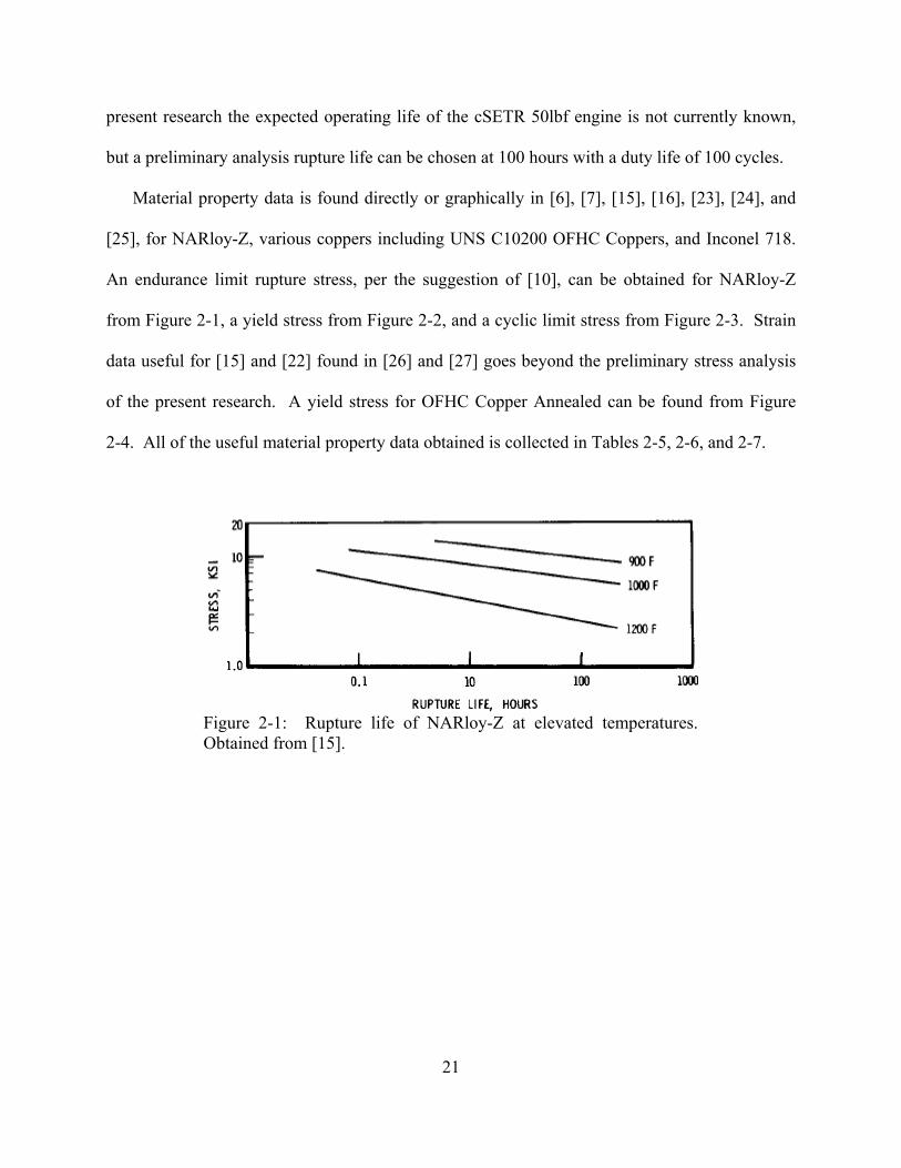
Material property data is found directly or graphically in [6], [7], [15], [16], [23], [24], and
[25], for NARloy-Z, various coppers including UNS C10200 OFHC Coppers, and Inconel 718.
An endurance limit rupture stress, per the suggestion of [10], can be obtained for NARloy-Z
from Figure 2-1, a yield stress from Figure 2-2, and a cyclic limit stress from Figure 2-3. Strain
data useful for [15] and [22] found in [26] and [27] goes beyond the preliminary stress analysis
of the present research. A yield stress for OFHC Copper Annealed can be found from Figure
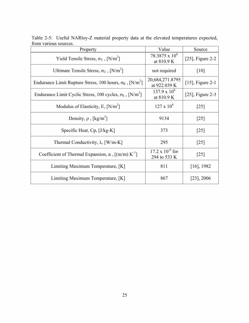
2-4. All of the useful material property data obtained is collected in Tables 2-5, 2-6, and 2-7.
Figure 2-1: Rupture life of NARloy-Z at elevated temperatures. Obtained from [15].

22
Figure 2-2: Stress-strain curves for NARloy-Z at various temperatures. Obtained from [25].

23
Figure 2-3: Cyclic stress-strain curve for NARloy-Z at 810.9 K. Obtained from [25].

24
Figure 2-4: Stress-strain curves for OFHC Copper Annealed at various temperatures. Obtained from [25].
25
Table 2-5: Useful NARloy-Z material property data at the elevated temperatures expected, from various sources.
Property Value Source
Yield Tensile Stress, σY , [N/m2] 78.3875 x 10⁶
at 810.9 K [25], Figure 2-2
Ultimate Tensile Stress, σU , [N/m2] not required [10]
Endurance Limit Rupture Stress, 100 hours, σR , [N/m2] 20,684,271.8795
at 922.039 K [15], Figure 2-1
Endurance Limit Cyclic Stress, 100 cycles, σE , [N/m2] 137.9 x 10⁶ at 810.9 K
[25], Figure 2-3
Modulus of Elasticity, E, [N/m2] 127 x 109 [25]
Density, ρ , [kg/m3] 9134 [25]
Specific Heat, Cp, [J/kg-K] 373 [25]
Thermal Conductivity, λ, [W/m-K] 295 [25]
Coefficient of Thermal Expansion, α , [(m/m) K-1] 17.2 x 10⁻⁶ for 294 to 533 K
[25]
Limiting Maximum Temperature, [K] 811 [16], 1982
Limiting Maximum Temperature, [K] 867 [23], 2006

26
Table 2-6: Useful Copper material property data at the elevated temperatures expected, from various sources.
Type of Copper Yield
Tensile Stress, σY , [N/m2]
Ultimate Tensile Stress, σU , [N/m2]
Melting Point,
Tm , [K] Source
Copper, Annealed 33.3 x 10⁶ 210 x 106 1356.35 to
1356.75 [24]
Copper, OFHC Soft 49.0 to 78.0 x 10⁶ 215 x 106 1356.15 [24]
Copper, OFHC Hard 88.0 to 324 x 106 261 x 106 1356.15 [24]
Copper, Annealed OFHC
29.915 x 10⁶ at 755.4 K
202 x 106 [25],
Figure 2-4
Copper, OFHC 1/4 Hard 310 x 106 330 x 106 [25]
Copper, OFHC 1/2 Hard 317 x 106 344 x 106 [25]
OFHC Copper 1355.56 [7]
OFE Copper 667, as limit fatigue max.
[6]
Table 2-7: Useful Inconel 718 material property data at the elevated temperatures expected, from [24].
Property Value Note
Yield Tensile Stress, σY , [N/m2] 980 x 106 at 923.15 K
Ultimate Tensile Stress, σU , [N/m2] 1100 x 106 at 923.15 K
Density, ρ , [kg/m3] 8190
Specific Heat, Cp, [J/kg-K] 435
Thermal Conductivity, λ, [W/m-K] 11.4
2.3 Cooling Channel Pressure Requirements
The presence of the enclosed passage walls affects the pressure of a moving fluid between
the inlet and the outlet, and thus the velocity and cooling performance, as explained in [12]. The
difference between the inlet and the outlet pressures is what drives the fluid to move in the

27
passage, but [10] states that a minimum difference is desirable and suggests a "smooth and
clean" inner surface. Various equations are given by [7], [10], and [14] for the hydraulic conduit
pressure drop with terms that are not easily determined, such as those involving surface
roughness. The influence of surface roughness as explained in [15] is that a more rough surface
increases the heat transfer coefficient but also increases the channel pressure drop, thus negating
any benefit.
The expander (or "topping") cycle engine is detailed in [10], [11], and [28], as one which
uses the heated and thus expanded coolant gasses exiting the cooling channels to drive turbine
pump machinery before being piped to the injector plate. The coolant path is shown in [7] as
first exiting the storage tank, then piped through a pump, then sent through a feed line, and
finally to the cooling channel inlet; incurring a 2.5% pressure loss in the feed line. At the outlet
of the channel for a non-expander cycle engine, the coolant/fuel is piped directly to the injector
plate before entering the combustion chamber.
Per [6], in order to prevent backflow into the channels from the combustion chamber, the
pressure at the exit of the channel must be greater than the combustion pressure. The
combustion pressure thus represents the minimum pressure allowed at the exit of the channel.
Also, the pressure loss in the channel must be accounted for such that the channel inlet pressure
is above the required exit pressure. Varying the cross sectional area along the length of the
channel, such as with the "continuous" shape of Figure 1-7, has a major impact on designing for
an optimal pressure drop from the inlet to the outlet.
Since the injector contributes an additional pressure drop for the coolant, the combustion
pressure actually represents the minimum pressure allowed at the exit of the injector, per [10]. A
rule-of-thumb value given for the injector pressure drop is 15% to 20% of the combustion

28
stagnation pressure. An alternative channel outlet pressure to chamber pressure ratio is assumed
by [12], without specifying the source of this pressure drop. Other criteria used in the past is
given in [16]:
a) minimum regenerative-coolant discharge pressure:
1) for liquid, p = 1.176 x chamber pressure
2) for gas, p = 1.087 x chamber pressure
b) maximum coolant velocity:
1) for liquid, v = 61 m/s
2) for supercritical gas, v = Mach 0.3
The criteria actually used in the analysis of [16] include a minimum channel outlet pressure
based on an allowable injector pressure drop, related to the chamber pressure. The minimum
allowable channel pressure drop from inlet to outlet is also a function of chamber pressure, and
values are given graphically.
The desired effect of maximizing the coolant temperature rise with an associated
minimization of channel pressure drop is studied in [6], [7], and [8]. The pressure drop is
determined in [6] with weakly defined equations written into a computer code. The results
indicated that for a "continuous" channel length shape, designing the HARCC to accommodate
the throat region always provides the highest benefit for temperature reduction. Unfortunately
the same channel cross section used along the length of the engine causes an undesirable high
pressure drop, but the continuous shape manufacturing method allows for later width increase
determination in the non-throat regions to give a beneficial low pressure drop. Optimizing the
uniform cross section channel for temperature reduction at the throat can thus be performed first,
and later the optimal cross sectional variation for pressure drop reduction can be determined.

29
The results also indicated that the optimal channel design used the "bifurcated" shape, but the
pressure drop was slightly higher than by not using that shape. The results of the "continuous"
shape showed a maximum coolant channel pressure drop of 5.0 x 10⁶ N/m2 for an engine much
larger than the cSETR 50lbf engine.
2.4 Aspects of Heat Transfer
The heat transfer in a regeneratively cooled rocket engine is based on the fundamentals of
heat transfer theory. The system can be divided into four control volumes for consideration of
heat transfer analysis, based upon the geometry of the cross section of coaxial shell designs. The
first: the heat transferred from the hot reacting combustion gasses comprised of the fuel and the
oxidizer components as they interact thermally with the combustion chamber wall. The second:
the heat transferred from the chamber-wall/inner-shell-structure to the cooling fluid inside the
channels. The third: the heat transferred from the inner shell to the adjoining portion of the
outer shell. The forth: the heat transferred from the outer shell to the external surroundings.
2.4.1 Basic Heat Transfer Theory
The basic fundamentals and theory of heat transfer are covered in detail within [13] and [29],
and specifically as related to rocket engines per [10], [14], [28], and [30]. The equations
required for the field of regenerative cooling are the same as those required for any heat transfer
application. Beginning from Fourier's Law, the generalized steady-state one-dimensional (1D)
equation for heat flux per unit area, q , is obtained with a coefficient term that gives its
generality. The coefficient term takes different definitions depending on which mode of heat

30
transfer is being modeled. For convective heat transfer between adjacent solid and liquid zones,
the coefficient is termed the "heat transfer coefficient" or "film coefficient", αg. For conductive
heat transfer through solids, the coefficient involves the material thermal conductivity and a
material thickness. The basic equations can also be rearranging for laminar or turbulent flow
considerations.
Special groupings of terms are often used to describe the degree of heat transfer, described in
[13] and [29]. For a fluid, the Nusselt number is the ratio of convection heat transfer to
conduction, and itself contains the heat transfer coefficient. For a solid/fluid interface, the Biot
number is the ratio of the internal thermal resistance of a solid to the external convective
resistance at the surface. The graphical explanation of the Biot number is informative for
cooling channel heat transfer if the contained terms can be directly manipulated.
2.4.2 Gas Side Heat Transfer
The heat transferred from the hot reacting combustion gasses to the chamber hot-wall is
termed the "Gas-Side Heat Transfer" in [10]. This combustion chamber wall surface area
adjacent to and facing the hot combustion gasses is equivalently termed in the literature as: "hot-
gas-side", "hot-gas-side wall", "hot gas wall", "chamber wall", "chamber inner wall" (sometimes
a term for the thinnest part of the inner shell), or similar.
The main mode of heat transfer is described by [10] as forced convection, since the
combustion gasses are traveling at a high velocity adjacent to the hot-wall. Three correlations
are given for the determination of the heat transfer coefficient, one is a "rough approximation",
the second is "a much used" equation of Colburn, and the third is the equation of Bartz. The
choice of which correlation to use is based on the available formulation. The "rough

31
approximation" equation contains terms which are not easily obtained without extensive
experimental data. The equation of Colburn takes the form of a Nusselt number, but the
dimensionless constant is not specified in [10] and the equation may therefore be unusable.
Finally, the equation of Bartz appears most complicated, but contains easily obtainable geometric
terms. Other terms can be obtained approximately through the use of other correlations given in
[10] or should be known for the particular engine.
For example, the ratio of specific heats is needed for the combustion mixture of O2 and CH4,
which are given individually by [31] at 300 K as: γO2 = 1.395, γCH4 = 1.299. The mixture
specific heat ratio can be found using a weighted sum of the partial molar fraction of individual
ratios, per [32]. Next, the specific heat of the mixture can be found using an equation given by
[10] and [31].
There is one temperature variable which is not specified in [10] for the Bartz equation, the
unknown inner wall temperature on the hot gas side. This temperature is both a design value to
be optimized and contained in the standard heat flux equation, causing some confusion. The
Bartz correction factor term contained in the Bartz equation is easily determined using the
provided graphs, seen in Figure 2-5, rather than a direct calculation. The Bartz equation seems
the preferred method of [10] to determine an approximate value for the heat transfer coefficient
along the chamber wall, with an unspecified "short form" used in [12].

32
Figure 2-5: Bartz equation correction factor values (σ) for various temperature and specific heat (γ) ratios at axial locations of ξ. ξ is the ratio of the local area to the throat area. ξC is in the chamber, one indicates the throat, ξ is in the nozzle. Obtained from [10].
The area ratio term in the Bartz equation indicates that the heat transfer coefficient will be
maximum at the throat region, and when applied in the heat flux equation suggests the maximum
temperature will also be experienced at the throat. The throat thus becomes the critical cooling
region where the heat flux will be highest, and where the number of cooling passages required
for a particular coolant flow rate should be determined. This is confirmed by [3], [6], [10], [12],

33
[18], [23], [28], [33], and [34].
The work of [28] gives valuable points of information which are essential to understanding
the heat transfer coefficient equations presented in other works. Specific terms are depicted in
the most basic dimensional analysis form for easy correlation. The calculation of the gas-side
heat transfer coefficient is by the Bartz equation, giving essential details about the equation that
are left out of other literary works. A figure plots experimental data and the Bartz equation to
confirm that the equation in the given form accurately predicts the heat flux along the
combustion chamber contour, peaking at the throat. With engine contour geometric terms
known and contained in the Bartz equation directly, the equation can be used to give the heat
transfer coefficient variation required if using a computational model of straight channels with
no curvature. The work of [30] notes that the Bartz equation is only valid in the region near the
nozzle throat.
A "modified" version of the Bartz equation presented in [7] and [14] more closely resembles
the Sieder-Tate or Dittus-Boelter relationships applicable to flow inside a tube or channel when
found in [13] or [29], and may not accurately represent the axial variation of hot-wall heat
transfer coefficient. A similar correlation used for the coolant side is mentioned by [14] but not
detailed. The validity of using this modified version can not be verified.
Carbon solids deposited on the interior combustion chamber walls by the combustion gas
products are also considered in [10] and [12] as a form of resistance to heat transfer, reducing the
effective coefficient value. The explanation as to whether this is a positive or negative condition
is not given in either work.
In consideration of the channel geometry cross section, [15] states that the influence of the
fin width to channel width ratio on the chamber wall temperature, for a constant coolant pressure

34
drop, is negligible for (2/3) ≤ (δf /w) < 2.
2.4.3 Regenerative Cooling and Coolant Side Heat Transfer
The heat transferred from the chamber-wall/inner-shell-structure to the cooling fluid inside
the channels falls under two headings in [10], "Regenerative Cooling" and "Coolant Side Heat
Transfer", with aspects of the previously mentioned heat transfer from the combustion gasses to
the chamber wall. The heat transfer mechanism is described as a generalized heat flow between
two fluid regions separated by a multilayer partition, utilizing multiple heat flux equations. This
is the same mathematical approach taken by [7], detailed in [13], and shown schematically in
Figure 2-6, where Taw represents the adiabatic wall temperature caused by the combustion
gasses, Twg represents the actual hot-wall temperature on the combustion gas side, Twc represents
the actual wall temperature on the coolant side, and Tco represents the bulk temperature of the
coolant inside the channel. The effects of the boundary layers, caused by the two moving fluids,
are shown to depict the change in temperature due to the heat transfer coefficients on the walls.
The heat transfer from the side wall of the coolant passage and not just the bottom wall, the "fin
effect", is not given with this description. The extended surface fin effect is derived in detail in
[13] and [29], which give equations for determining the material conductive height necessary for
efficient heat extraction through convection to the surrounding fluid. The theory required to
obtain the fin height is based upon longitudinal heat conduction in a rod, with corrections to
account for a non-adiabatic tip. The concept is utilized with lack of detail in [7], [12], and [14].

35
Figure 2-6: 1D heat transfer schematic representation of regenerative cooling. Obtained from [10].
When analyzed separately from the combustion gas region, the heat transfer from the channel
wall into the adjacent coolant falls under the category of "Coolant Side Heat Transfer" in [10].
Equations are given which describe the heat transfer coefficient for two cases of coolant state
properties, important when considering non-ideal fluid behavior. The Sieder-Tate equation for
turbulent heat transfer to liquids flowing in channels is for the case of nonboiling subcritical
temperature, and subcritical to supercritical coolant pressures. This equation takes the form of a
Nusselt number, and contains an unknown constant which is specific to the coolant being
analyzed. One sample calculation in [10] suggests the use of this equation for the propellant RP-
1 and uses unspecified experimental data to give the constant as C1 = 0.0214. The generalized
presentations of the equation in [13], [29], and a partial form in [35], give the constant as C1 =
0.023. The work of [7] is concerned with methane directly and gives the constant as C1 = 0.027,
but the source used for the equation is extremely old and the equation has slightly different
exponent values. The second equation given by [10] is for the case of a vapor-film boundary
layer where the coolant is at supercritical pressure and temperature, suited for hydrogen per

36
Figure 1-9 which shows the supercritical operating conditions. The choice of which of the two
equations to use for methane is not clear since a boiling phase change could occur. An equation
to estimate the coolant system capacity is also given.
The work of [16] gives an equation for the heat transfer to the homologous propane as
assumed characterizing that for methane, in the form of a Nusselt number. The equation is not
fully explained and given by a reference which at times gives unclear information and
mathematical relations, thus the equation is not considered useful.
The text [28] gives an equation based on theory and other researcher formulations to directly
predict the coolant side film heat transfer coefficient in cooling tubes, in a form which allows
application to non-circular channels. With this form, comparisons and proper utilization can be
achieved with equations presented in other literary works lacking detail.
2.4.4 Solid to Solid Heat Transfer
The heat transferred from the inner shell to the adjoining portion of the outer shell by direct
contact conduction between two solid regions is described in [13] and [29]. The fin effect is
linked to the solid-to-solid heat transfer since the bottoms of the fins mathematically touch and
physically join the chamber wall at a control volume boundary, and the tops of the fins are what
is touching the outer shell at a physical boundary. The typical assumption of an adiabatic fin tip
per [7] is not valid as a proper boundary condition in a CFD simulation since heat can be
transferred, and [13] gives the required mathematical adjustment for a non-adiabatic tip.

37
2.4.5 Outer Shell Heat Transfer
The heat transferred from the outer shell to the external surroundings can be considered as
the final form of heat removal for the coaxial shell engine design. Taking this form into
consideration is important for proper definition of numerical boundary conditions. Radiation
cooling is only discussed in [10] in relation to nozzle extensions, but is detailed in general by
[13] and [29]. The heat flux equation requires a coefficient value depending on the material and
surface finish. The emissivity of a wall surface made with oxidized (or rough surfaced) nickel is
given as ext = 0.41 at 373 K by [29].
The work of [11] discusses the topic of engine testing. Static ground testing at sea-level
conditions is one method mentioned, even used in [18], which involves natural or forced
convective cooling in atmosphere. Equations to determine the required mean heat transfer
coefficient over a flat plate from [13] can be used for an idealized flat outer portion of an engine.
Testing in an altitude chamber for engines designed to operate in thinner atmospheres is also
mentioned in [11]. Thus considering the operating conditions of an engine being utilized for
interplanetary travel in the vacuum of space, as in the current research, it is practical to consider
radiation cooling as important on the outer shell. The work of [7] considers this, but makes the
assumption of an external temperature of absolute zero as well as an over simplified heat flux
balance.
2.5 Material Loading, Stress, and Failure
Sufficient structural strength is necessary in the design of a regenerative cooling system, as
the system is also integrated with the design of the engine itself. The focus of the present

38
research is on the cooling performance, but a structural design is required to possess at least the
minimum strength necessary in terms of mechanical and thermal loads.
An analysis of the expected working loads on the engine due to the cooling system is
required and discussed in [10]. Typical recommended safety factor criteria are given for the
design limit load, yield load, ultimate load, and endurance limit. As explained, the endurance
strength limit of a material should be used in place of the ultimate strength value in cases of
cyclic loading operation, typical of the multiple starts and stops of a rocket engine. Many failure
modes are evaluated and discussed, the complexity of which suggests that a detailed analysis is
required for proper final designs. For a preliminary stress analysis though, only static and some
cyclic failures can be considered to determine a baseline structure for an engine.
The design loading criteria of [10] is contradicted in [15], which states that some components
are designed within a yield strength criterion of an increased multiple of the yield stress for the
material, 1.1 x σy. Designing a part by artificially increasing (rather than decreasing) the
material limits would decrease the ability of the part to handle loading, resulting in a weaker
design. The criteria of [10] increases the expected loading for a consistent material property,
resulting in a stronger and thus more desirable conservative design.
In structural terms, [10], [15], and [18] describe the throat as the critical design location
where maximum stress will occur, and at the inner chamber wall surface of the inner shell. The
throat is thus in the area with the shortest life expectancy, and where material damage will likely
begin. An equation given for the coaxial shell stress goes beyond the scope of a preliminary
analysis, and furthermore includes terms that are unknown before a numerical analysis is
performed. Other equations found in [10] are not sourced but are discovered to be the same as
the basic mechanics of materials theory of [17], which itself states that the same theory be used

39
in many other areas of rocket engine stress design.
In a more general sense, [10] continues by explicitly stating that the coolant pressure causes
only a circumferential hoop stress in the outer shell. Also, the inner shell experiences both a
compressive stress and a thermal stress. The compressive stress is caused by the pressure
differential between the coolant and combustion chamber, whereas the thermal stress is caused
by the temperature gradient across the chamber wall. These stresses can also be analyzed using
the methods of [17].
Since the chamber wall represents the thinnest portion of the inner shell, [15] and [7]
describe the minimum allowable thickness as directly related to the channel width when
considering pressure stresses and failure. The generalized failure mode descriptions of [10] are
expanded upon in [15] to a more detailed duty cycle equipment life analysis with focus on this
thinnest location. For a preliminary stress analysis, the accumulation of stress rupture creep
damage and low cycle fatigue damage are important. These damages are ignored by [7].
For the consideration of stress rupture creep damage, the endurance limit determination using
[15] and Figure 2-1 for the NARloy-Z material at a chosen rupture life allows a design of the
channel width and chamber wall thickness which minimizes failure in this manner. Fatigue
specimen data showed that this damage is minimized by using the narrow channel width of 1.016
mm reported, with a resulting increase in the number of possible life cycles.
For the consideration of low cycle fatigue damage, an equation is given by [15] which allows
for the calculation of the bending pressure stress over the mid-channel due to the pressure
difference between the coolant and combustion chamber; the stress being highest at the mid-
channel. Rearrangement of this equation allows for a design of the channel width and chamber
wall thickness which minimizes failure in this manner, with proper selection of material stress

40
limits. An equation is also given for the calculation of the shear pressure stress, which is
maximum near the interface of the channel and side wall due to the sudden change in wall
thickness. Both equations are similar; the difference being a second order effect of channel
width to chamber wall thickness ratio for the bending equation, and a first order effect for the
shear equation. When this ratio is greater than one, the maximum pressure stress is thus in
bending. When the ratio is less than one, the maximum pressure stress is in shear. Angular
shear strain data is not given in [15] to use the shear equation directly.
The experiments conducted in [18] were performed with the purpose of determining the
cyclic loading fatigue damage and life at the throat of three AR channel geometries, with results
shown in Table 2-8. These results and the associated geometries from Table 2-2 allow optimal
design ratios to be determined and selected for other engine designs.
Table 2-8: Structural results for channels tested in [18].
Configuration Number
AR at Throat Structural Result
1 0.75 average life design;
eventual material failure
2 1.50 long life design;
eventual material failure
3 5.00 no failure design
Thermal loads are also a major concern for rocket engines. The scope of [16] is on the
unique requirements for regeneratively cooled chambers operating at low thrusts and high
chamber pressures, giving the following expected temperatures for an engine of slightly higher
performance than the cSETR 50lbf engine:
a) differential between hot-wall and outer shell; strain considerations: 700 K
b) range for hot-wall, O2 cooled: 728 K to 806 K

41
c) range for channel lower wall, O2 cooled: 478 K to 533 K
The works of [15] and [22] explain that the temperature gradients caused by hot combustion
gasses and cold coolant on opposite sides of the same wall, as well as between the hot-wall and
outer shell, lead to shorter material life from strain effects even if the regenerative cooling
process can reduce the hot-wall temperature below that of melting.
The validity of the approach of [7] to determine the thermal stress for the coaxial shell
construction can not be verified with the information presented, nor using the cited equation
sources of [10] and [15] as suggested. Many material and engine parameters are required with
the equations of [10], basically identical for coaxial shell as well as tubular stress, and
interestingly do not involve the channel width parameter reported by [7] as the result of the
approach. A maximum channel width of 2.54 mm is given, but is questionable.
The results of [18] show that increasing channel AR has an effect of decreasing the hot-wall
temperature significantly. The highest temperature was found to be located on the hot-wall
adjacent to the channel centerline, with a temperature minimum underneath the fin structure.
This 2D phenomena is confirmed by [13] and [28]. Additionally, [18] states that a further
reduction of the temperature can be achieved if AR's higher than 5.0 are used. The explanation,
explained in [13] and later confirmed by [8], is that the cooling channel surface area is much
larger than the combustion chamber hot-wall surface area for HARCC applications, which acts to
expel a higher quantity of the absorbed heat. Moreover, using HARCC to cause lower material
temperatures can reduce the possibility of thermally induced plastic ratcheting. Thinning of the
chamber wall adjacent to the channels, as well as the through crack failure depicted in Figure
1-8, are indicative. A doubling of the thermal cycle life was found by [6] as possible by reducing
the throat hot-wall temperature from the conventional maximum of 778 K to below 667 K.

42
Further insight into the criteria with which to judge material failure can be gained using the
limit analysis of engineering structures and indeterminate beams presented in [36]. In limit
analysis, an acceptable maximum load can be ascertained for a structure which is permitted to
develop a reasonable plastic deformation with only the minimum number of plastic hinges
allowed before a mechanism is formed. Despite the deformation, the structure may be able to
withstand greater loads before complete failure is achieved, and can be designed using those
greater loads. Utilizing limit analysis allows for an elastic-limit criterion to be easily set for a
preliminary stress analysis with the methods of mechanics of materials for indeterminate beams
per [17]. The more difficult and involved analysis of elastic-plastic material behavior, as done
by [5] and [18], can be avoided. The criterion is either the actual limit load or a bracket of it.
2.6 Using Methane as the Coolant and Fuel
The use of methane as the coolant and the fuel, with liquid oxygen as the oxidizer, in a
bipropellant rocket engine system presents challenges which are not as prevalent when using
other coolants, as discussed in the few literary works which actually consider methane.
Furthermore, most literary works such as [6], [7], and [12] are concerned with engines with
much higher thrust and chamber pressures than the cSETR 50lbf engine. Works which consider
lower thrusts are [16] and [35], however [35] is a text book with focus on established techniques
so does not consider methane, whereas [16] is a research study which does.
The work of [12] studies the cooling capabilities of light hydrocarbon fuels including
methane for supercritical high coolant pressure operation, but involves fluorinated oxidizers.
Equations and graphs are provided to calculate certain state properties of the coolant system
involving enthalpy considerations, also considered in [23], which may require reformulation to

43
consider non-fluorinated liquid oxygen. Some conclusions as given may not fully apply to
simple methane/oxygen. The cooling capabilities for methane are shown to be good for high
engine thrust levels and high combustion chamber pressures, but not for low chamber pressures
due to the small range of liquid operating conditions before phase change occurs. In the
subcritical low pressure operation, [8] confirms that boiling phase change must be allowed for
methane. For a low thrust and low chamber pressure engine such as the cSETR 50lbf engine, the
phase change phenomena presents a design challenge for the typical cooling operation near the
critical point seen in Figure 1-9.
Additionally, [16] determined that only a limited number of specific impulse, chamber
pressure, and thrust operating points are possible with methane and oxygen. Methane as a
coolant operating in the supercritical single-phase state was considered to have the following
qualities in comparison to using oxygen as the coolant:
a) for thrust levels lower than 100lbf: not recommended, but oxygen capability is low
b) for combustion chamber pressures lower than 3.45 x 10⁶ N/m2: allowed
c) does not cause copper oxidation, in contrast to oxygen above 589 K
d) peak engine performance at oxidizer to fuel mixture ratio of 3.5 ± 0.5
The minimum allowable channel pressure drop from inlet to outlet is also given, and can be read
from Figure 2-7 at the chamber pressure of the cSETR 50lbf engine as ∆P = 600,000 N/m2.

44
Figure 2-7: Allowable cooling channel pressure drop for O2/CH4 systems as a function of chamber pressure. Obtained from [16].
Decomposition of hydrocarbon fuels and the depositing of carbon atoms on the engine
surfaces, "coking", is a concern at high temperatures and investigated by [12], [16], [23], and
[37]. Methane in particular is not subject to decomposition, and temperature limits are usually
given based on approximate failure limits for structural engine components. Values include: a
range of 873.15 K to 1173.15 K (for pure methane, reducing with impurities), 978 K, and a range
of 1033 K to 1367 K.
An additional limiting temperature is placed by [12] in consideration of coolant film effects,
of 1036 K. Restrictions on the optimal operating pressures for methane are also given, but the
values are for a much higher thrust than the cSETR 50lbf engine. A coolant inlet temperature to
the channel is also suggested to be at 5.6 K above the normal freezing point for any fuel. For

45
methane in particular, [16] gives a typical inlet temperature of 112 K, and [7] gives the pressure
and temperature conditions of Table 2-9 for an application with a feed line connecting the
turbopump exit to the channel inlet. The computational models of [8], however, attempt to
reproduce actual methane working conditions by using the values in Table 2-10.
Table 2-9: Pressure and temperature conditions of methane found from the analysis of [7].
Location Pressure, [N/m2] Temperature, [K]
Turbopump Exit 12,996,617.4976 118.0556
Channel Inlet 12,672,563.9048 116.6667
Channel Outlet 11,514,244.6796 526.2222
Table 2-10: Pressure and temperature conditions of methane used by [8].
Property Value Channel Inlet Stagnation
Temperature, T0 , [K] 130
Channel Inlet Stagnation Pressure, P0 , [N/m2]
9 x 10⁶
Channel Outlet Static Pressure, P, [N/m2]
7 x 10⁶
More temperature limits and values for methane are found in [10], [38], and [16]. An upper
temperature limit of 450 K is imposed on methane for using the expander cycle to drive turbine
pumps. The methane channel outlet temperature range is reported to be 328 K to 478 K, with
maximum allowable bulk temperature limit of 478 K to 533 K due to rapid decrease in density.
Given point property values are shown in Table 2-11.

46
Table 2-11: Various point property values for methane.
Property Value Source
Freezing Point, [K] 88.706 [10]
Boiling Point, [K] 110.928 [10], 1967
Boiling Point, [K] 112 [16], 1982
Critical Pressure, [N/m2] 4.598 x 10⁶ [16]
Critical Temperature, [K] 191 [16]
Dynamic Viscosity, μ, [kg/m-s] 16 x 10-6, 473.15 K [38]
Dynamic Viscosity, μ, [kg/m-s] 18.5 x 10⁻⁶, 573.15 K [38]
Knowledge of the expected combustion temperature for oxygen and methane (O2/CH4) at the
proper mixture ratio is essential to define an important boundary condition and directly effects
the design of the cooling system, but a value is not readily found in literature. To give an
estimate of the typical temperatures found in combustion, although not necessarily representative
of the value for O2/CH4, [10] and [15] provide the values for fluorine-oxygen (OF2) oxidizer with
methane fuel burning at 3977.59 K, and oxygen with hydrogen burning at 3611.11 K. An exact
value is still required, which can be obtained with the suggestion of [6]. The analysis employed
an ideal combustion condition with no losses, resulting in the hottest combustion gas temperature
possible and a more conservative approach to the definition of cooling requirements. This
suggests that the maximum adiabatic, or a suitable equilibrium, flame temperature be calculated
using the methods of advanced thermodynamics based on [32] and [39]. Needed reference
information found in [28] and [40] is shown in Table 2-12. Equations to calculate the needed
ideal gas specific heats are in [28].

47
Table 2-12: Useful heats (enthalpies) of formation at 298.15 K from [28], and compound molar masses (molecular weights) from [40].
Compound Formula h °f , [kJ/kmol] MM (MW), [kg/kmol]
Methane (g) CH4 -74,873 16.0426
Oxygen (g) O2 0 (diatomic molecule) 31.998
Carbon Dioxide (g) CO2 -393,522 44.009
Water (g) H2O -241,827 18.0148
Carbon Monoxide (g) CO -110,530 28.01
2.7 Computational Modeling and CFD
The complex nature of three dimensional (3D) fluid flow can be modeled mathematically
using low order 1D methods to gain approximate results which are often suitable for a simple
flow application. As described in [41], fluid dynamics theory is based upon a combination of
mathematics and experimental refinement. For regenerative cooling in particular, [42]
additionally notes that a 1D analysis using Nusselt type empirical correlations is typical which
provides about ±20% error. The universal character of CFD to directly model physical
phenomena without adjustment correlations from experimental data is promoted.
When fluid dynamics theory is combined with computers, larger and more complex flow
applications can be solved with a faster turnaround, with the added possibility of more accurate
results. Before a computational fluid dynamics (CFD) computer model is built however, an
understanding and application of the basic theory is required to ensure that the CFD results
obtained will be reasonable.
The fundamental conservation laws of physics used to describe generalized fluid motion can
be found in [41] and [43], and are very complex in their 3D form. They include conserving:
mass, termed the continuity equation; linear momentum, beginning as Newton's second law of

48
motion; and energy, termed the first law of thermodynamics. Of particular interest are the
momentum and energy equations when formulated in the proper manner. The momentum
equations lead to the complex Navier-Stokes equations, which are important to describe 3D fluid
flow. The energy equation gives the ability to describe heat transfer, boundary layers, and fluid
turbulence. The complexity of these equations often requires many discretizations in order to
obtain analytical solutions. Applying additional flow theory and equations then allows for the
proper use of CFD.
An important definition when describing fluid boundary layers adjacent to solid walls is the
non-dimensional distance y+, derived and discussed in [13], [41], and [43]. The distance is
sometimes termed as part of the "law of the wall" when surface roughness effects are involved,
and applied to the channel fluid domain in a computational model.
As explained in [41], applying the y+ concept to CFD allows a computationally efficient
method to discretize a fluid domain next to a wall boundary into a computational mesh. A
formula in terms of y+ is given to calculate the nearest mesh grid point actual distance from the
wall. Adhering to the absolute minimum criteria that y+ > 11.63 ensures that the mesh is not
prohibitively dense, since resolving all the details in a turbulent boundary layer are usually not
necessary. The result would be extremely long computational times with little added benefit, as
seen in [44]. The discussion of CFD solution stability analysis in [45] from a purely
mathematical standpoint leads to the understanding that using excessively small meshes, with y+
below the absolute minimum criteria, may create the situation of stiff mathematical matrices
which are difficult to solve. The usage of y+ by [8] is not detailed and the value used "of order
1" is questionable.
Various references give preferred ranges for designing the near-wall mesh such that the y+

49
value falls within the fully turbulent region of the boundary layer on a smooth wall, shown in
Table 2-13. Still adhering to the absolute minimum y+ criteria, [3], [33], [41], [44], and [46]
describe a grid refinement mesh sensitivity investigation for improving the accuracy of any
particular CFD application.
Table 2-13: Preferred smooth wall y+ ranges of various references.
Reference Ranges Reference Note
[41] 30 < y+ < 500
[44] 22 < y+ < 100 gives best results
[43] 70 < y+ < 400
[47] and [48] 30 < y+ < 300 preferably near the lower bound
[13] y+ > 60 fully turbulent region
[49] y+ > 30 fully turbulent region
With the adherence to the y+ criteria and ranges, the "wall function approach" is then used to
represent the effect of the wall boundaries with additional "wall function" equations. Details and
various treatments are given in [41], [47], and [48]. The "standard wall functions" are applicable
to the y+ ranges of Table 2-13. The handling of near-wall bounded turbulent flows is linked to
the manner by which the flow turbulent viscosity is modeled.
Changes in the turbulent kinetic energy, "k", and turbulent dissipation rate, "ε", of fluid and
computational flows is explained in [41] and [47] through the use of mathematical turbulence
models. Minor variations on the classic two equation realizable "k-ε model" with standard wall
functions are widely used in literature and only valid for the fully turbulent region, per [3], [44],
and [49]. However, the more complex seven equation linear pressure-strain "Reynolds Stress
Model" is explained as more general and potentially very accurate. The choice between the two
is not clear and must be investigated through a turbulence sensitivity study.
The work of [41] states that distributions of the k and ε values must be defined as boundary

50
conditions to the turbulence models at the inlet of internal flows. Equations to calculate crude
approximations of these values are given, equivalent to those in [47], and require a length scale
and turbulence intensity factor. Suggested values for intensity are given by various references,
shown in Table 2-14. Rough-guess inlet values for k and ε are shown by [46] which can be used
for comparison purposes only: k = 0.09 m2/s2, ε = 16 m2/s3. But, the results should not be
sensitive to these inlet values because most of the turbulence is generated in the internal flow
boundary layers downstream.
Table 2-14: Suggestions for turbulence intensity factor of various references.
Reference Ti , or as I Reference Note
[41] 1% to 6 % typical values
[44] 5% for a combustion chamber
[47] I < 1% "low", used if the upstream flow is under-developed and undisturbed
[47] 1% < I < 10% "medium", used if the upstream flow is
fully developed
[47] I > 10% "high"
The use of the Bartz equation for the combustion gas side heat transfer coefficient has been
explained to give the variation required along the hot-wall when using a computational model of
straight channels with no curvature. A computational model can thus relate to the experimental
method of [18] which uses straight channels in a plug-nozzle engine design where the
combustion chamber is formed from a cylinder, with a water cooled center body inserted which
has the curvature. The location of minimum distance between the cylinder and the center body
as seen in cross section creates the throat. Viewing the Bartz equation, the mathematical
representation of this chamber geometry is the same as a typical cone nozzle. Flow curvature

51
effects in the HARCC were not determined in [18] or the computational models of [8],
suggesting that temperature effects can be investigated before curvature effects are included.
For physical internal channel flow, [13], [29], and [31] describe a non-steady-state entrance
length upstream of the thermally and hydrodynamically fully developed region. For
computational internal channel flow, [22] and [41] describe an adiabatic flow entrance length
upstream of the heated channel section to be investigated. A length of ten times the heat transfer
section length is found, but the equations are more useful. The work of [14] prefers unspecified
"sufficient" entry lengths instead of a calculation.
The entrance length concept involves the addition of extra channel length upstream of the
inlet to the flow area of interest, for the purpose of allowing the flow to become
hydrodynamically fully developed in an adiabatic manner prior to the flow area of interest. A
new inlet is created upstream of the original inlet for experimental work. In CFD simulations,
the new inlet is the CFD inlet, and the original inlet becomes a simple measured distance
downstream of the CFD inlet to denote the location of the beginning to the flow area of interest.
Adding the entrance length to a CFD model allows for a numerically pre-developed flow.
Related to the regenerative cooling channel concept, the CFD inlet can be thought of as the inlet
to the feedline which pipes the coolant to the cooling channel inlet. The cooling channel inlet is
thus the beginning to the flow area of interest, and where the adiabatic portion ends and heat
addition begins.
Various computer codes are available to model fluid dynamics and heat transfer. The work
of [16] modifies the ALRC SCALER thermal design computer program into the 1981 form
called SCALEF, and gives some of the program details. The program uses 1D heat transfer
theory involving a form of the Dittus-Boelter equation to calculate the hot-gas side heat transfer

52
coefficient. The equation is given in generalized form by [13] and [29], but for applying on the
coolant side.
Many researchers use the two related computer codes RTE and TDK, for example [3], [6],
and [23]. RTE is a 3D thermal evaluation code for rocket combustion chambers, while TDK is a
2D non-equilibrium nozzle analysis and performance code. Other codes and subroutines, like
the ROCCID rocket combustion injector analysis code, are possible for implementation. Despite
being specific to cooling channels and rocket engines, the codes as written have limitations like
assuming a uniform cross sectional temperature in the HARCC in contrast to references in [6]
and the results of [8], [33], and [50]. Still, the theory used in the codes relevant to rocket engines
can be a valuable resource for comparing or beginning a more generalized CFD software
simulation that overcomes the limitations.
Many researchers, for instance [7], [8], [14], [49], and [50], chose to write their own
computer codes based on 1D heat transfer theory. Some implement other resources for fluid and
combustion properties, like the NIST chemistry web-book, the NASA Thermochemistry code, or
the NASA Chemical Equilibrium Analysis (CEA) program. Then, the computational results
obtained in that manner may be compared to multiple ANSYS CFD computer models in 2D for
separate solid and fluid regions, but not in a 3D integrated manner.
At the beginning of a design, it may be sufficient to consider only steady-state effects and
conditions. This was the focus of the experimental work of [18] and the computational work of
[3]. To add flexibility, generalized CFD software can also be used to obtain transient results if
needed at a later time.
The commercially available CFD software ANSYS FLUENT, now up to version 12.1, has
been widely used for many applications. It is mentioned in [41] and used by [3], [33], [42], [44],

53
and [46]. Additionally, [42] uses two separate software, Advance/FrontFlow/red and CRUNCH
CFD, for comparison of results. The extensive details of the FLUENT software are given in the
documentation of [47], [48], and [51] showing that the underlying theories of heat transfer and
fluid flow from many other references are implemented using the finite volume approach.
Information is given in terms of proper utilization of CFD discretizations, as well as solution
strategies for complex models. One particular strategy is to start the simulation at a low order
discretization, then switch to a higher order for increased solution accuracy. With the proper
application of boundary conditions and settings, the FLUENT software can be used for
generalized problems involving ideal or real gasses, steady state or transient solutions, fluid flow,
heat transfer, turbulence, solids, and with the "interface" method a coupled simulation involving
fluids together with solids using the additional information from [52]. A thorough understanding
of the governing equations is necessary for proper utilization of the software and confidence in
the results. Some limitations of FLUENT are found through experience: certain licenses are
limited to the use of 512,000 total mesh cells which limits mesh density, and the software prefers
flows in the positive x axis direction though not required. Of particular interest in [48] is the
statement that the value of y+ is not a fixed geometric quantity but is solution dependent, and
therefore should be adjusted by performing a mesh & turbulence sensitivity study prior to the
main simulations. Using the methods above for determining y+ does however allow an initial
mesh to be determined.
Turbulence model application in FLUENT is given detail in the documentation, noting that
the "realizable" k-ε model has substantially better performance than the "standard" version.
There is a slight disparity between the documentation and the software with which of the default
model constants of Table 2-15 are used and able to be adjusted, noted in the table. Default

54
solution control factors, as well as under- and explicit-relaxation factors, as used in FLUENT are
given in Table 2-16.
FLUENT also supplies an extensive built-in Material Property Database which can be
adjusted to the user's specific application. The useful quantities are given in Table 2-17.
Table 2-15: FLUENT turbulence model default constants and suggestions, per [47], [48], [51]. Note: values include standard wall functions and viscous heating.
Parameter realizable k-ε model
Note for k-ε linear pressure-strain Reynolds Stress Model
Note for RSM
Cμ 0.09
C1ε 1.44
shown in equations in [47] and [51] but not
in software
1.44
C2ε 1.9 given as "C2" in
[47] and [51] 1.92
Pressure Strain C1-PS
1.8
Pressure Strain C2-PS
0.6
Pressure Strain C'1-PS
0.5
Pressure Strain C'2-PS
0.3
TKE Prandtl Number, σk
1.0 1.0 value is 0.82 in
[47] and [51] but 1.0 in software
TDE Prandtl Number, σε
1.2 1.3 value is 1.0 in
[47] and [51] but 1.3 in software
Energy Prandtl
Number, Prt 0.85 0.85
Wall Prandtl Number
0.85 0.85
Full Convergence
Criteria Required
10-6 10-4

55
Table 2-16: FLUENT default solution control, under-, and explicit- relaxation factors, per [47], [48], and [51].
Factor Value Reference Note
Courant (CFL) Number 200 may need 20 to 50 for
complex 3D cases, per [51] Momentum 0.75 may need ~0.5, per [48]
Pressure 0.75 may need ~0.2, per [48]
Density 1 may need <1.0, per [48]
Body Forces 1
Turbulent Kinetic Energy, k 0.8 may need ~0.5, per [48]
Turbulent Dissipation Rate, ε 0.8 may need ~0.5, per [48]
Turbulent Viscosity 1
Reynolds Stresses (RSM only) 0.5
Energy 1 may need <1.0, per [48]
Table 2-17: Useful FLUENT Material Property Database values, from the software interface and through [48] referenced files.
Property Methane, CH4 Nickel, Ni Copper, Cu Air
Density, ρ , [kg/m3] 0.6679 8900 8978 1.225
Specific Heat, Cp, [J/kg-K] 2222 460.6 381 1006.43
Thermal Conductivity, λ, [W/m-K]
0.0332 91.74 387.6 0.0242
Dynamic Viscosity, μ, [kg/m-s]
1.087 x 10⁻⁵
Molar Mass / Molecular Weight, MM, [kg/kgmol]
16.04303
Reference Temperature, [K] 298.15 ~298.15
Critical Temperature, [K] 190.56 9460
Critical Pressure, [Pascal = N/m2]
4599000 1.08 x 10⁹
Critical Specific Volume, [m3/kg]
0.006146 0.000391

56
Prior to using the FLUENT CFD software, an additional piece of software is required to
create the geometry and mesh. The software GAMBIT has been used, particularly by [3], mainly
because it was packaged with older versions of FLUENT. The software Altair HyperMesh is a
useful choice as it provides the functionality to organize 3D features in specific ways which are
required by FLUENT. Some important limitations of HyperMesh are found through experience:
can only handle three decimal places, can only allow eleven characters total in a type-in box, and
can not handle placement of nodes closer than about one half millimeter. Due to the values
possible for insertion, this limits the overall significant figures to a maximum of six.
2.8 Ideal Versus Real Gas Modeling
The wide variation possible in the state properties of a fluid presents challenges in the
calculation of property behavior undergoing any process. Simplifications are often made and
utilized for approximate results from the real gas behavior toward an ideal gas solution. For the
most accurate results, a real gas solution is desired but is not always available. In the field of
computational fluid modeling, additional challenges arise from the implementation of the real
gas models.
The complex real gas fluid behavior is introduced in [10], [12], and [13] as it relates to heat
transfer. The process of nucleate and film boiling phase change, and its effect on the heat
transfer behavior of a coolant, is examined mainly from an experimental standpoint. Little
information is given for the calculation of the behavior without requiring experimental data.
Such experimental data is not typically available prior to a numerical simulation as the purpose
of numerical simulations is to obtain the preliminary results. Multiple numerical simulations are
thus required with a range of adjustments to the mathematical model, for experimental validation

57
later. The two heat transfer coefficient equations mentioned previously, the Sieder-Tate and
vapor-film equations, are the only tools available in [10] to model the real behavior of a coolant.
These equations require the user to assume or otherwise determine the fluid behavior beforehand
with the purpose of choosing which equation to use, or require both equations to be used for later
validation.
Cryogenic hydrogen is a typical fuel used in bipropellant rocket engines due to its well
behaved thermodynamic behavior during engine operation, and investigated in many works
including [8], [10], [12], [14], [15], [18], [23], [33], and [49]. The state property transition for
hydrogen is solely in the supercritical region where the pressure is far from the critical point on a
pressure-temperature state diagram, as explained in [8]. Figure 1-9 shows that the state property
transition for methane during typical regenerative cooling operation is much closer to its critical
point in the transcritical region where phase change is a likely possibility. This adds to the
complexity involved in the design, use, and optimization of the channels, as well as the
computational modeling of the methane coolant behavior. The work of [8] goes as far as
utilizing a specialty made CFD code in an attempt to overcome the real behavior limitations of
more general software.
Various modeling options are available in the generalized FLUENT CFD software to
represent the behavior of both ideal and real gasses, described in [47], [48], and [51]. The
computational complexity and expense increases when moving from the relatively simple ideal
gas model to other more complicated models, noted by [49], peaking at any real gas model due
to the increased number of terms in the equations. The real gas behavior is desired for
optimizing a channel design, however one may not be easily available for implementation in the
computational model chosen. For instance, the phase change which is likely to occur with

58
methane, as seen in Figure 1-9 and suggested by [34], does not allow the use of the standard
built-in FLUENT real gas modeling techniques and would require a user-defined model.
Despite the real gas software limitation of FLUENT, the well known ideal gas equation can
be used to give preliminary and estimated results of the real gas behavior for later comparison.
Ideal versus real behavior was investigated by [50] for instance, showing that the real behavior
dominates along much of the channel and should not be ignored. This is particularly true for
methane based on the analyses of [12] and [23], and enthalpy/energy techniques have been used.
2.9 The cSETR 50lbf Thrust Engine
Geometry and operating parameters for the cSETR designed 50lbf engine of Figure 1-10
were obtained from [9], described by [11] as a conical type nozzle engine integrated with the
combustion chamber as one piece. The effects of the wall contour on the cooling properties or
channel flow characteristics may be strong due to the small radius of curvature and sharp angle
of attachment with the chamber. Modeling straight channels with no curvature or angle is
possible with the Bartz equation, mentioned previously, if the true cooling channel length along
the curved surface of the combustion chamber wall, a "corrected" length rather than the axially
projected length, is used.
The fuel feed system for the cSETR 50lbf engine is not currently finalized, but [11] suggests
pump instead of pressure feeding for regenerative cooling due to the increased propellant tank
pressure required to overcome the channel pressure drop in a pressure fed system. The increased
pressure requirement also increases the structural weight of the tank, which is not favored. The
work of [16] examines various engine cycles and feeding system methods, which should be
analyzed for the proper choice involving methane with the help of [35]. The expander cycle
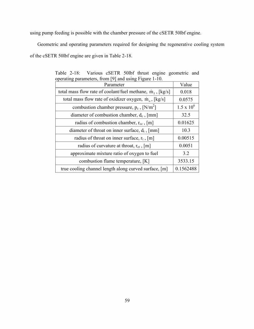
59
using pump feeding is possible with the chamber pressure of the cSETR 50lbf engine.
Geometric and operating parameters required for designing the regenerative cooling system
of the cSETR 50lbf engine are given in Table 2-18.
Table 2-18: Various cSETR 50lbf thrust engine geometric and operating parameters, from [9] and using Figure 1-10.
Parameter Value
total mass flow rate of coolant/fuel methane, fm , [kg/s] 0.018
total mass flow rate of oxidizer oxygen, om , [kg/s] 0.0575
combustion chamber pressure, pc , [N/m2] 1.5 x 10⁶
diameter of combustion chamber, dc , [mm] 32.5
radius of combustion chamber, rcc , [m] 0.01625
diameter of throat on inner surface, dt , [mm] 10.3
radius of throat on inner surface, rt , [m] 0.00515
radius of curvature at throat, rct , [m] 0.0051
approximate mixture ratio of oxygen to fuel 3.2
combustion flame temperature, [K] 3533.15
true cooling channel length along curved surface, [m] 0.1562488

60
CHAPTER 3
MATHEMATICAL THEORY OF REGENERATIVE COOLING
This chapter presents the mathematical theory required for the design and optimization of
regenerative cooling passages to be used for rocket engine applications, as used in the present
research. The basic theory behind the required equations is given when available to indicate the
origins and limitations. The chapter outline and section layout used previously is closely
followed for convenience due to the many theoretical aspects considered. Additional detail for
equations and theory which are related but not directly manipulated in the present research may
be found in the references discussed in the literature review.
3.1 Cooling Channel Pressure Relationships
Certain pressure limitations must be adhered to for the proper operation of regenerative
cooling channels. To prevent backflow into the channels, the pressure of the coolant when it
reaches the combustion chamber must be larger than the combustion pressure. The combustion
pressure thus represents the minimum allowable coolant pressure.
When the injector pressure drop is considered, the minimum allowable channel outlet
pressure can be calculated using:
dropcout PpP min (1)
where: cp = combustion chamber pressure, [N/m2],
Pdrop = minimum allowable pressure drop across the injector, [N/m2].
Options for determining the injector pressure drop are given by [10] and [16]:

61
75.0cdrop pP , (2)
or,
cdrop pP 2.0 . (3)
Alternately, [12] gives a direct equation to calculate the minimum allowable channel outlet
pressure:
cout pP 2min . (4)
Three values for the minimum allowable channel outlet pressure are available for consideration.
The channel itself also contributes a pressure drop to the coolant. Upstream, the minimum
allowable channel inlet pressure can be calculated by adding the channel pressure drop, P , to
the minimum outlet value in a similar fashion:
PPP outin minmin . (5)
Quick estimation of P can be performed without an equation if adequate literature reference
information is provided.
3.2 Theory of Cooling System Heat Transfer
The theory used to describe a regenerative cooling system can be divided into separate
control volumes of the basic heat transfer theory and discussed separately. This is possible
mainly due to the use of CFD software which couples the equations automatically. The separate
control volumes allow for various definitions of CFD boundary conditions, and simplifies the
task.

62
3.2.1 Basic Heat Transfer Theory
The basic equations for heat flux form the fundamentals of the heat transfer theory required
to describe regenerative cooling. In the equations, the coefficient terms are the most important
and usually difficult to define for a generalized system, but take focus for mathematical
simulations. Figure 2-6 and the information in [28] can be used to describe the theory.
The convective heat transfer rate at the fluid-solid interface of the combustion chamber
gasses and hot-wall is described by the heat flux equation in the form:
whgghw TThq 0 (6)
where: hg = hot-gas heat transfer film coefficient on the hot-wall, [W/m2-K],
T0g = stagnation (total) temperature of the free stream combustion gasses, used with
little loss of accuracy from the more accurate adiabatic wall recovery
temperature Taw in Figure 2-6, [K],
Twh = Tgw of Figure 1-6 = Twg of Figure 2-6 = hot-wall temperature, [K].
Definition of the hot-gas heat transfer film coefficient, hg , is required to describe the gas side
heat transfer.
The conductive heat transfer through a solid wall is given by the 1D heat flux equation in the
form:
wcwhw
w TTL
q
(7)
where: w = thermal conductivity of the wall material, [W/m-K],
L = wall thickness, [m],
Twc = wall temperature of the colder surface, [K].
Knowledge of the material gives the thermal conductivity. The application of this equation can

63
occur in multiple locations of the cooling channel cross section, as well as with extended fin
surfaces. Solid-to-solid heat transfer is accomplished when two solids adjoin at an interface and
the heat flux exiting one material equals that entering the other, with an equal temperature value
at a firmly joined interface.
The convective heat transfer rate at the solid-fluid interface of the chamber wall, or fin, and
cooling fluid is described by an equation of the same form as Equation (6):
cowcgc TTq (8)
where: g = convective heat transfer coefficient on the channel wall, [W/m2-K],
coT = temperature of the free stream coolant, as in Figure 2-6, [K].
Definition of the channel heat transfer coefficient, g , is essential to design the extended fin
surfaces located between each channel passage.
Certain term groupings are often seen and analyzed. Just as the Nusselt number (Nu)
describes heat transfer into a fluid enclosed within a passage by relating the heat transfer
coefficient g with the properties of the passage, [13] describes the heat transfer from a wall
into the fluid and relates g with the properties of the wall through the use of the Biot number
(Bi). Comparing the two numbers, heat transfer can be increased by the adjustment of certain
parameters to increase Nu and Bi as much as possible:
a) b
g DNu
1) increase the heat transfer coefficient
2) increase passage diameter or hydraulic diameter, D, which in effect increases the
surface area

64
3) decrease the thermal conductivity of the coolant, b
4) for a specific fluid, b is fixed for ideal conditions, so g and D should be as large as
practical
b) f
og LBi
1) increase g ; which is the same g value as for Nu
2) increase wall thickness, oL , to allow for better conduction
3) decrease the thermal conductivity of the wall material, f
4) for a specified wall material, f is fixed, so g and oL should be as large as
practical
In effect, the heat transfer coefficient is a function of the wall surface area, and shows the
advantage of HARCC. The high value for g leads to a thin thermal boundary layer and
indicates good heat transfer, while a small g leads to a thick layer and bad heat transfer.
HARCC increases the surface area over which a thin boundary layer can exist and operate.
The external radiation properties of real bodies are based on the Stefan-Boltzmann Law. The
radiation heat flux equation uses terms that are easily defined and do not require extensive sub-
calculation as is the case for the convective heat transfer coefficients hg and g . The form of the
equation most useful to later CFD application is per [48]:
44wSBextr TTq (9)
where: ext = emissivity of the external wall surface, a material property,
SB = 5.670 x 10-8 = Stefan-Boltzmann constant, [W/m2-K4],

65
T = temperature of the radiation sink on the exterior of the domain, [K],
wT = surface temperature of the wall, [K].
3.2.2 Gas Side Heat Transfer
The convective coefficient required to describe the heat transfer on the combustion chamber
hot-wall must take into account the variation in combustion gas properties as they travel in the
combustion chamber, past the throat, and out the nozzle. When combined with Equation (6), a
peak in heat flux at the throat must be seen, according to many literature sources. The Bartz
equation, mainly a function of the local cross sectional area, accomplishes the required behavior:
9.01.08.0
0
0
6.0
2.0
2.0
**
*Pr*
026.0
A
A
r
D
c
pc
Dh
ct
pg , [W/m2-K]. (10)
The correction factor for property variations across the boundary layer is given by:
2.0
2
2.08.0
2
0 21
121
21
121
1
MMTT
g
wh . (11)
The known terms of Equations (10) and (11) are:
D* = engine throat diameter of the inner surface, [m],
p0 = pc = stagnation (total) pressure of the combustion chamber at the location of the
nozzle inlet, [N/m2],
rct = radius of curvature of nozzle contour at throat along centerline axis, [m],
2*4
* DA
= cross sectional flow area at throat, [m2],

66
24
dA
= axial flow chamber inner surface cross sectional area at a local value
of the inner diameter d; area under consideration along chamber axis; varies
with position from the injector, to the combustion chamber, to the throat, to
the nozzle exit along the engine centerline axis; the ratio of the local area to
the throat area in Figure 2-5 is formed by
*A
A ; [m2],
= exponent of viscosity-temperature relation; 6.0 for diatomic gasses and
gives the values for plotted in Figure 2-5, allowing graphical
determination of rather than direct calculation,
sysm
Apc
** 0 = characteristic velocity, [m/s],
oxidizerfuelsys mmm = propellant consumption steady mass flow rate, [kg/s],
Twh = Twg of Figure 2-5 = hot-wall temperature, can use an assumed average
reference value from literature, [K],
gT0 = (Tc)ns of Figure 2-5 = nozzle stagnation inlet temperature, or chamber total
temperature, of the free stream, [K],
nsc
wg
g
wh
T
T
T
T
0
, knowledge of this ratio allows the graphical determination of
from Figure 2-5,
γ = specific heat ratio of the combustion mixture prior to the reaction.
Methods of advanced thermodynamics per [31] and [32] can be used to determine some of
these quantities. The chamber total temperature, gT0 , can be found from a calculation of the
adiabatic flame temperature of the combustion components for the particular oxidizer and fuel

67
used in the engine. The specific heat ratio of the combustion mixture prior to the reaction, γ, is
found by taking the average weighted sum of the partial molar fraction of individual reactant
specific heat ratios, using the reaction equation coefficients:
ii
iii
avgmixture n
n . (12)
Interpolation is necessary when extracting values from Figure 2-5 for between the plotted
curves, performed by the linear equation with terms defined in Figure 3-1:
01
0100 xx
yyxxyy . (13)
For example if the required mixture is not exactly a value as shown, the subscript 0 terms would
be the pair of values from one curve of γ to give the lower bound of , while the subscript 1
terms are from an adjacent curve giving the upper bound.
Figure 3-1: Linear interpolation terms of Equation (13).
The unknown terms of Equations (10) and (11) are:
M = local Mach number variation along the nozzle,

68
Pr0 = Prandtl number of the combustion gasses, stagnation conditions,
0 = dynamic viscosity of the combustion gasses, stagnation conditions, [kg/m-s],
cp 0 = specific heat of the combustion gasses, stagnation conditions, [J/kg-K].
A reconciliation of the unknown terms can be done using the equations provided in [10] and [31]
for approximate results. For the Prandtl number:
59
4Pr
(14)
where mixture from Equation (12). For the dynamic viscosity, a unit conversion is necessary
to evaluate:
6.05.0100 106.46 TMW , [lb/in-sec] (15)
where: MW = molecular weight (molar mass) of combustion products, [lb/mol],
T = temperature of the gas mixture, [R],
the required units are [kg/m-s].
The combustion gas specific heat is obtained with:
10
R
cp , [J/kg-K] (16)
where the specific gas constant of the combustion gas products is calculated from:
MW
RR U (17)
and: RU = 8.314 = universal gas constant, [kJ/kmol-K],
MW = molecular weight (molar mass) of combustion products (representative values
seen in Table 2-12), [kg/kmol].
All of the terms in the Bartz equation are defined, and the heat transfer coefficient variation
along the wall in the centerline axial direction is able to be determined using the contour

69
variation of an engine cross sectional geometry.
3.2.3 Coolant Side, and Solid to Solid, Heat Transfer
The extended surfaces theory of [13] begins with the 1D steady state heat conduction in a rod
that allows heat to be released from the outer surface. The rod tip is assumed insulated, so that it
does not allow heat to be released. The rod material is homogeneous, surrounded by a fluid at
constant temperature. The heat transfer at the rod surface is assumed constant, though generally
not true. A 3D image is formed by adding a depth and a thickness to the rod, but maintaining the
1D effect of the temperature only changing along the length of the rod. With the length of the
rod defined as the height, and thickness as the width, a fin of rectangular profile is created. For
the most beneficial fin effect, the heat flow released from the fin surface area, excluding the
insulated tip, into the surrounding coolant should be as large as possible. The maximized energy
balance of heat flow entering the fin at the base and exiting through the surface results in a
criteria which determines the optimal fin height based on material and flow conditions:
ff
fh2
4192.1 (18)
where: h = fin height from base to tip, [m],
f = constant convective heat transfer coefficient at the fin surface, [W/m2-K],
f = constant thermal conductivity of the fin material, [W/m-K],
f = fin width, constant from base to tip, [m].
As the heat released from the fin tip is required for proper CFD boundary conditions, a
mathematical adjustment is necessary. The h in Equation (18) is replaced with a corrected fin
70
height, which contains the originally defined fin height, and an incremental height that provides
the surface area required to release the same amount of heat as would be released at the tip:
2
fc hhhh
(19)
where: ch = corrected fin height, [m],
2
fh
= incremental height addition, [m].
By assuming that the surface area of the fins is much larger than the surface area of the ground
between any two fins, Af >> Ag , then the convective heat transfer coefficient at the fin surface is
assumed approximately equal to that at the ground, gf . Combining and rearranging, the
equation for the fin height becomes:
2
24192.1
2/1
2/1 f
f
gfh
. (20)
Various options are available for determining the convective heat transfer coefficient
required. The first is the film coefficient of [28], applicable to the coolant side heat transfer in a
tube or channel:
67.02.0
1 023.0
b
p
bpg
cDGcG
, [W/m2-K], (21)
where: b = dynamic viscosity of coolant, [kg/m-s],
bpc = specific heat of coolant, [J/kg-K],
b = thermal conductivity of coolant, [W/m-K],
subscript b = quantity is evaluated at bulk mean temperature of coolant.
Equation (21) contains the following three relationships. The hydraulic diameter for a

71
rectangular channel is given by:
hw
hw
P
AD
24 , [m], (22)
where: A = channel cross sectional area, [m2],
P = channel perimeter, [m],
w = channel width, [m],
h = channel height, [m].
The average mass flow per unit area is given by:
2
2
244
hw
hwm
D
muG c
c
, [kg/m2-s], (23)
where: = coolant density, [kg/m3],
u = coolant velocity, [m/s],
overbar indicates the average of the quantity over a domain.
The mass flow rate per cooling channel is given by:
c
tc n
mm
, [kg/s], (24)
where: fuelt mm = total coolant mass flow rate of the cooling system, [kg/s],
cn = total number of cooling channels about the engine circumference.
Also, the circumferential length can be matched to a linear representation of the length used for
all of the channels by the relationship:
wnr fco 2 (25)
where: or = throat radius to the outer chamber wall surface (bottom of cooling channel).
The second option for determining the convective heat transfer coefficient required is the

72
Sieder-Tate relationship version of [10], in the form of a Nusselt number, using suggestions from
literature:
14.0
4.08.01 PrRe
w
bCNu
(26)
where: b
g DNu
2 = Nusselt number,
C1 = 0.023 = constant depending on coolant, per [13], [29], [35],
b
Du
Re = Reynolds number,
b
pb c
Pr = Prandtl number,
w = coolant dynamic viscosity at coolant-side wall temperature, [kg/m-s],
equation is valid for: 0.5 < Pr < 120, 104 < Re < 105, L/D ~ 60.
The third option for determining the convective heat transfer coefficient required is the
Sieder-Tate relationship version of [7]:
14.0
3/18.03 PrRe027.0
w
b
b
g DNu
. (27)
The forth option is brought to account for the similarity between the second, Equation (26),
and the third, Equation (27). The film coefficient from [28] of the first option, Equation (21),
can be compared to the vapor-film boundary layer heat transfer coefficient of [10]:
55.0
2.0
8.03/22.0
4 Pr029.0
wc
cobpg T
T
D
Gc , [W/m2-K], (28)
where: coT = coolant bulk temperature, [K],
wcT = coolant-side wall temperature, [K].

73
It should not be surprising that four equations were found which determine the convective
heat transfer coefficient, as [28] suggests only minor refinements to the same underlying theory
result in the various options reported in literature, and all equations are tied together through the
Nusselt number. For example, [35] gives an equation that does not contain any
refinement/correction terms. The above equations should thus give similar results, but which
particular equation gives the most accurate results is not clearly stated in the literature which is
why their results must be compared numerically. However, Equation (21) from [28] couples the
underlying theory with experimental knowledge involving tubes with an explicitly given
hydraulic diameter conversion to rectangular channels. Equation (21) can then be assumed to
give the most useful values with the highest degree of certainty over the other equations, due to
insufficient information presented in [7], [10], [13], [29], and [35].
The coolant dynamic viscosity at the elevated coolant-side wall temperature can be
determined through Sutherland's Equation:
ST
TC
2/32 (29)
where: = dynamic viscosity [kg/m-s] at temperature T [K],
C2 = Sutherland Equation constant,
S = Sutherland Equation constant.
The constants can be determined using two different dynamic viscosities at two different
temperatures in tabulated reference data for a particular coolant. Knowing the constants then
allows the desired dynamic viscosity to be calculated at the desired temperature.
74
3.2.4 Outer Shell Heat Transfer
Heat transfer from the outer shell must be considered in experimental and CFD cases where,
in contrast to [7] and cooling fin theory which assume an adiabatic fin tip, all energy transferred
across the chamber wall is not absorbed by the coolant in an idealized situation. The tip of the
cooling fin adjoins the bottom of the outer shell and allows for a solid-to-solid heat transfer
mechanism. The temperature differential between the coolant and the engine exterior also
promotes the transfer of heat through the outer shell. For exterior temperatures likely much
lower than the combustion temperature, heat must be allowed to exit the outer shell into the
surroundings. The surrounding fluid or vacuum is not considered part of the cooling system, but
must be included for proper CFD boundary condition definition. According to the literature on
the topic, two main outer shell heat transfer mechanisms are useful to be analyzed: convection to
atmosphere, and radiation in vacuum.
The first boundary condition option is convection to atmosphere. The required heat transfer
coefficient, , can be estimated by using the technique of idealizing a thin strip of the outer
surface, located on top of one cooling channel, as a flat plate when the curvature is "corrected"
by flattening rather than projecting the length onto the centerline axis. The assumption of
longitudinal frictionless flow and [13] are used to determine the mean heat transfer coefficient:
La
wmm
2
, [W/m2-K], (30)
where: = thermal conductivity of surrounding atmosphere, [W/m-K],
pca = thermal diffusivity of surrounding atmosphere, [m2/s],
cp = specific heat of surrounding atmosphere, [J/kg-K],

75
= density of surrounding atmosphere, [kg/m3],
wm = constant average velocity of surrounding atmosphere, [m/s],
L = true cooling channel length along the surface of the chamber wall, [m].
Relatively stagnant atmospheric conditions can be assumed for the velocity.
The second boundary condition option is radiation to vacuum. No terms in the radiation heat
flux of Equation (9) require extensive calculation through sub-equations when reference
information is available.
3.3 Theory of Material Loading, Stress, and Failure
The rocket engine and regenerative cooling system require structural analysis and design in
multiple ways for multiple locations. Analogous mathematical representations can be formed
from the theories of [17] and [36].
3.3.1 Cylindrical Pressure Vessel Analogy
The combustion chamber of a rocket engine can be viewed as a cylindrical pressure vessel.
For known pressure, radius, and material, a manipulation of the circumferential hoop stress
equation allows the required wall thickness to be determined depending on the application:
rpt , [m], (31)
where: p = applied internal pressure, [N/m2],
r = inner radius, [m],
= material static yield or ultimate stress, [N/m2].
The longitudinal axial stress, and stresses at the inner and outer surfaces, are calculated by other

76
formula which result in smaller thicknesses, would give an under-designed engine, and are not
considered.
3.3.2 Fixed End Beam With Uniform Pressure Load Analogy
The span of chamber wall length between two adjacent fins, at the bottom of a particular
cooling channel, can be idealized as a fixed-end statically indeterminate beam with a uniform
pressure load q acting over the entire length L. The situation is depicted in Figure 3-2.
Figure 3-2: Statically indeterminate fixed-end beam representation of chamber wall span between two fins, at the bottom of one cooling channel.
The uniform pressure load as shown is a force per unit length, and can be converted to an
effective pressure due to the combustion chamber pressure and the cooling channel pressure.
The effective pressure is depicted in Figure 3-3.

77
Figure 3-3: Illustration of effective pressure acting on the chamber wall.
The effective pressure is a force per unit area, assumed constant, and acts over the x direction
length of the channel. Calculation thus becomes:
cineff pPp min (32)
where: mininP = assumed maximum constant pressure experienced along the length of the
channel, also equals the cooling channel minimum allowable inlet
pressure, [N/m2],
cp = combustion chamber pressure, assumed constant along the length of the
chamber, [N/m2].
The uniform pressure load is thus equivalently:
chaneff Lpq (33)
where: Lchan = actual length of the channel, equivalent to the "corrected" length of the
chamber, [m].
Viewing the beam representation in Figure 3-4 depicts the orientation for the bending
moment of inertia.

78
Figure 3-4: Beam representation as seen along the y axis.
For a rectangular cross section, the bending moment of inertia with the origin at the centroid,
with respect to the x axis, is given by:
12
3tLI chan (34)
where: t = chamber wall thickness as depicted in Figure 3-4, [m].
Because the failure with respect to deflection is unknown, the Euler-Bernoulli theory of beam
bending can be used. The moment in the beam is shown in Figure 3-2, and given by:
12
2LqM . (35)
The flexure formula then gives the normal stresses due to the bending moments:
I
zM (36)
where: 2
tz = the distance in the z direction for the positive maximum stress on the face
of the beam, [m].

79
Combining Equations (35) and (36) using limiting criteria gives a maximum allowable pseudo-
beam length when solved for L:
eff
Y
ptL
2minmax (37)
where: Lmax = maximum allowable channel width, [m],
tmin = minimum allowable chamber wall thickness, [m],
Y = chamber wall material yield stress, [N/m2].
Interestingly, the result is in the same form as the partial equation found in [16] that was not
adequately defined to be used in itself. Even though the derived formulation appears consistent,
not enough information is given to use the related data of [16] with a high degree of confidence.
3.3.3 Fixed End Beam With Uniform Temperature Load Analogy
Continuing the idealization of a fixed-end statically indeterminate beam, consideration of
temperature effects can be included. For the regenerative cooling channel, a temperature
differential exists between the combustion chamber hot gasses and the cooling channel coolant.
This fluid temperature differential causes a material temperature differential between the hot-
wall and the channel lower wall. Instead of Equation (35), the moment in the beam of Figure 3-2
is now:
t
TIEM
(38)
where: = coefficient of thermal expansion of the material, [m/m-K],
E = modulus of elasticity of the material, [N/m2],
I is per Equation (34),

80
T = material temperature differential, [K].
Combining with the flexure formula of Equation (36) eliminates the chamber wall thickness
parameter t, thus a maximum temperature differential allowed before yielding occurs can be
solved for:
E
T Y
2
max . (39)
3.3.4 Column Subject To Buckling Analogy
The outer shell of a coaxial engine is typically made of a material with a much higher
strength than the inner shell. As such the cooling fins typical of HARCC applications, made of
the lower strength inner shell material, may be subjected to loads which could cause buckling.
The higher strength outer shell acts as a rigid support, fixing a fin at the top against rotation and
translation, as depicted in Figure 3-5. The fin is viewed as a column with the lower end fixed
against rotation, and no differential pressure load between adjoining channels.
Figure 3-5: Cooling fin represented as a column subjected to buckling loads.

81
The bending moment of inertia for a rectangular cross section, with the origin at the centroid, is
again with respect to the x axis. The beam representation in Figure 3-6 depicts the orientation
when viewed down the column.
Figure 3-6: Column representation as seen along the z axis.
The bending moment of inertia equation is per:
12
3chanf
fin
LI
. (40)
The critical load which causes buckling is thus calculated using the equation:
2
24
fin
fincr L
IEF
. (41)
The combustion chamber pressure shown in Figure 3-5 acts over the idealized fin base area,
being the base of the column representation, and can be equivalenced into a point force with:
chanfcc LpF . (42)
If the combustion chamber force is set as the critical load which causes buckling, Fc = Fcr, a ratio

82
can be found which relates the maximum allowable fin height to the minimum allowable fin
width, for the condition that buckling will occur beyond those values. Equating Equations (41)
and (42), using (40), results in:
cf
fin
p
EL
3min
max
. (43)
3.3.5 Recommended Criteria For Loads
The work of [10] provides an alternate basis for the definition of static pressure loading
conditions which allow for a strong design. The values obtained in this manner are then
combined with material stress limits and Equation (31) to determine the geometric features
required to withstand the loads. For regenerative cooling systems, the process must be used
twice to accommodate the chamber wall of the inner shell, and then the outer shell.
The process begins with a definition of various load types, all of which are pressures for the
particular application to rocket engines. Load Type A, LA, is defined as the working load under
normal steady-state operating conditions, and is typically set by the design. Load Type B, LB, is
defined as the working load under transient operating conditions of normal engine start and stop,
which can be idealized as equivalent to LA if information is not available. Load Type C, LC, is
defined as the working load under occasional transient operating conditions of irregular starts.
Load Type D, LD, is defined as the mandatory malfunction load which must be taken into
account in instances of continued operation during other component failures. The mathematical
relationship is as follows:
AL set by design, (44)
AB LL , (45)

83
AC LL 1.1 , (46)
AD LL 225.1 . (47)
The limit loads, LL, are defined next for each load type:
AAL LL 2.1 , (48)
BBL LL 2.1 , (49)
CCL LL 1.1 , (50)
DDL LL 0.1 . (51)
The design limit load, LDL, is selected as the maximum of the limit loads:
DLCLBLALDL LLLLL ,,,MAX . (52)
Finally, loads which may cause yielding, LY, or ultimate failure, LU, can be determined:
DLY LL 1.1 , (53)
DLU LL 5.1 . (54)
The material stress limits used with these loads are the associated yield, Y , or ultimate, U ,
strengths. For parts subjected to cyclic loading, the material endurance limit stress, E , is used
in place of the ultimate stress, if available.
3.3.6 Simplified Theory of Cyclic Loading Stress Analysis
Cyclic loading can be analyzed in a simplified manner for a preliminary stress analysis of the
chamber wall using the methods and equations of [15]. Both low cycle fatigue and creep rupture
life can be considered.
For the consideration of low cycle fatigue, noting that the bending pressure stresses are

84
maximum at the mid-channel, a design ratio can be found through rearrangement of the given
equation. The result is interestingly of the same form as Equation (37):
hotwallcoolant
B
PPt
w
2
(55)
where: w = L of Figure 3-2 = channel width, [m],
B = material bending stress maximum, [N/m2],
Pcoolant = loading on the coolant side of the chamber wall, [N/m2],
Photwall = loading on the hot-wall, [N/m2],
t
w =
max
t
w =
t
wmax =
mint
w for yield or ultimate P's and B .
In the rearranged equation, the loading parameters can be taken as either the yield or the ultimate
values, used with the associated yield or ultimate material stress values.
For the consideration of creep rupture life, Equation (55) is used with the rupture life stress in
the place of B to give the design ratio.
3.4 Using Methane as the Coolant and Fuel
The use of oxygen and methane (O2/CH4) in a combustion process at the proper mixture ratio
requires knowledge of the expected chamber temperature. Not only is the temperature essential
for defining an important numerical boundary condition, but it is needed in the utilization of the
Bartz equation to determine the convective heat transfer coefficient variation on the hot-wall.
Because a temperature value is not readily found in literature for this oxidizer/fuel combination,
the chamber total temperature, gT0 , can be determined from a calculation of the adiabatic flame
temperature of the combustion components per the methods of [32].

85
The oxidizer to fuel mixture ratio is used to setup a reaction equation of the form:
COOHCOOCH 2224 edcba (56)
where the small letters represent the molar coefficients, and carbon monoxide is included to
account for the possibility of incomplete combustion. Determination of the adiabatic flame
temperature is based on the energy rate balance heat transfer equation:
RP HHQ (57)
where: Q = rate of heat transfer at the combustion chamber control volume boundary, [J],
HP = enthalpy of the products, [J],
HR = enthalpy of the reactants, [J].
For the adiabatic condition, Q = 0, so that HR = HP. The heat transfer equation becomes, on a
molar basis and summed for all products and reactants in terms of enthalpy:
i
Piii
Rii hnhn (58)
where: ni = coefficient of the reaction equation for the ith component, per mole of fuel,
[kmol],
ih = specific enthalpy for the ith component, per mole of fuel, [kJ/kmol].
The specific enthalpy for compounds not at the reference temperature of 298.15 K is found by
adding the enthalpy of formation (representative values seen in Table 2-12) and the change:
hhh f (59)
where: fh = enthalpy of formation for a compound at the standard state, [kJ/kmol],
Tch p = specific enthalpy change between the standard state and the state of
interest, [kJ/kmol],

86
pc = specific heat for a particular compound, [kJ/kmol-K],
15.298 TT = change in the temperature from the standard state to the state of
interest, [K],
T = temperature at the state of interest, [K].
For compounds at the reference temperature, 0h . Also, since Tcc pp , then
dTTcdh p , which can be written for substitution as:
2
1
T
T p dTTch (60)
where: T1 = initial temperature of the compound before the reaction, [K],
T2 = final temperature of the compound after the reaction, [K].
The heat diagram method is used in the determination of temperature limits for Equation (60).
The required ideal gas specific heats are calculated using the equations provided in [28], shown
in Table 3-1. Finally, substitutions are made into Equation (58) to determine the required flame
temperature.
Table 3-1: Ideal gas specific heats of expected combustion reactants and products, from [28].
Gas Tcc pp , [kJ/kmol-K]; 100
T , [K]
CH4 -672.87 + 439.74 θ0.25 - 24.875 θ0.75 + 323.88 θ-0.5
O2 37.432 + 0.020102 θ1.5 - 178.57 θ-1.5 + 236.88 θ-2
CO2 -3.7357 + 30.529 θ0.5 - 4.1034 θ + 0.024198 θ2
H2O(g) 143.05 - 183.54 θ0.25 + 82.751 θ0.5 - 3.6989 θ
CO 69.145 - 0.70463 θ0.75 - 200.77 θ-0.5 + 176.76 θ-0.75

87
3.5 Theory Required for Computational Modeling and CFD
A thorough knowledge of the assumptions and implications involved in any computational
modeling technique are essential. For a pre-packaged CFD software program, additional
knowledge is necessary to avoid the "black box, junk-in & junk-out" effect typical of less
experienced users. In so doing, proper determination of the computational mesh, turbulence
model parameters, and flow entrance length are necessary.
3.5.1 Mesh Considerations, "y" Values, Etc.
Determination of the proper mesh density is essential for obtaining reasonable results. The
initial details can be calculated, but must then be adjusted through a mesh sensitivity study
involving trial runs of the desired simulations.
Prandtl's "Mixing Length Theory" from the definition of shear stress, a part of the "Law of
the Wall", forms the basis for determining a limit mesh size in order to realistically resolve
boundary layer details at a wall. The wall friction velocity is defined per [13] and [43] as:
0w (61)
where: 0 = shear stress at the wall due to the constant of integration of the momentum
equation for the boundary layer in a steady-state, turbulent, stratified flow of a
channel with vanishing pressure gradient, [kg/m-s2],
ρ = density of the fluid, [kg/m3].
Also, the non-dimensional distance from the wall is defined as:
yw
y (62)

88
where: y = dimensional distance from the wall, [m],
= kinematic viscosity of the fluid, [m2/s].
Combining Equations (61) and (62) results in the same equation as in [41] for y+:
0y
y (63)
which can be written in terms of mesh nomenclature as:
wpy
y
(64)
using: py = distance of the near-wall computational grid node to the solid surface,
equivalent to the distance between the wall and the center of a CFD finite
volume mesh element (i.e. the center of a FLUENT or HyperMesh mesh
element), see Figure 3-7, [m],
0 w = shear stress at the wall, [kg/m-s2].

89
Figure 3-7: Distance of the near-wall computational node to the solid surface for a 3D CFD element.
For the near-wall, viscous, linear to 1st order, flow region the shear stress can be represented as:
p
pw y
u
(65)
where: = dynamic viscosity of the fluid, [kg/m-s],
pu = average velocity for turbulent flow at the grid node near the wall, where
viscous shear dominates, [m/s].
In order to use known values for the calculation of a mesh size, note that by definition the
viscosities are related to the density by:
, (66)
and solve for the distance py by substituting Equation (65) into (64) to obtain:

90
pp u
yy
2
. (67)
By assuming an average, set the quantity Guup , and substitute in Equations (22), (23),
and (24) to obtain the final form for the distance between the wall and the center of a CFD finite
volume mesh element:
t
c
p m
nhwhw
yy
4
22
2
. (68)
Equation (68) is useful for particular channel cross sectional geometries which have been
previously determined, and subject to the y+ criteria restrictions of Table 2-13.
Because the above formulation for py is not valid beyond the inner region of the boundary
layer, using Equation (68) to directly determine the number of mesh elements to place along the
height and width of a channel is not valid. It must be used only for the wall adjacent mesh
element height, vertically or horizontally for a rectangular channel, and from that the total
number can be determined with consideration for biasing possibilities. Biasing is the progressive
stretching of adjacent elemental heights or widths as the element position progressively gets
farther away from the wall. Also, the equation can not be used to determine the mesh density for
the channel lengthwise direction, in the direction of the mean flow.
The maximum number of mesh elements theoretically required in either the vertical or
horizontal direction can be found by using the minimum allowed value of y+, resulting in the
minimum allowed distance minpy , even if biasing is used. For no biasing, using a mesh with
equal element heights or widths for the entire span of the vertical or horizontal direction, the

91
maximum number of elements can be calculated by the following. The maximum number of
associated mesh elements in the vertical direction, for no biasing, is given by:
min
max 2 py
hV
. (69)
The maximum number of associated mesh elements in the horizontal direction, for no biasing
and using the same value of minpy , is given by:
min
max 2 py
wH
. (70)
These values are also related to the number of channels, nc, as the channel height and width are
functions of nc per Equations (20), (25), and associated.
Although not related to y+, the channel lengthwise mesh should ideally be fine enough to
resolve the variation in heat transfer coefficient along the hot-wall as calculated by Equation
(10). The number of lengthwise elements can be calculated by:
e
T
L
LL (71)
where: LT = total length of the channel, [m],
Le = length per element for a non-biased mesh, [m].
3.5.2 Turbulence Model Parameters
Both the k-ε and Reynolds Stress turbulence models in a CFD simulation require initial
guesses of the inlet boundary conditions for the turbulent kinetic energy, k, and turbulent
dissipation rate, ε, parameters.
An explicit calculation of the inlet distribution of turbulent kinetic energy for internal flows

92
is performed per [41] and [47] by:
22
3IUk avg (72)
where: Uavg = reference average flow velocity, [m/s],
I = turbulence intensity of Table 2-14.
Combining Equations (72), (22), (23), and (24) results in the usable form:
2
22
2
4
2
3
hwhw
n
mIk
c
t , [m2/s2], (73)
where the CFD channel inlet density, , can be estimated for the coolant using Equation (17)
with the coolant molecular weight, and the ideal gas law:
inlet
inlet
TR
p (74)
using: inletp = channel pressure at the CFD channel inlet, [N/m2],
inletT = channel temperature at the CFD channel inlet, [K].
In a CFD model, a pre-inlet entrance length is added upstream of the inlet to the actual
modeled cooling channel of interest. The modeled cooling channel is where heat is added and
what is being simulated. The CFD channel inlet is thus the inlet to the channel in the CFD
model, and is upstream of the inlet to the modeled channel which is being considered.
Knowledge of the modeled channel inlet pressure per Equation (5), pin, can be used to determine
the channel pressure at the CFD channel inlet, pinlet, using the same method as before. Using the
feedline pressure loss (drop) ahead of the actual channel inlet from [7] of 2.5% formulates the
following relation in terms of the CFD channel inlet pressure:

93
isof% ,
fdinlet pp 025.0 , (75)
where fdp is the feedline pressure drop between the CFD inlet and the modeled inlet. The CFD
and modeled channel inlet pressures are thus related by:
fdininlet ppp , (76)
and upon substitution of Equation (76) into (75) for inletp and rearrangement gives a relation for
the feedline pressure drop in terms of the modeled channel inlet pressure:
fdin p
p
025.01
025.0 . (77)
Substitution of Equation (77) back into (76) results in the desired relationship needed for
Equation (74) and thus calculation of the turbulent kinetic energy per Equation (73):
ininlet pp
025.01
025.01 . (78)
Next, the length scale for fully developed turbulent pipe flows is calculated per [41] and [47]
using the hydraulic diameter of Equation (22) by:
Dl 07.0 . (79)
Finally, an explicit calculation of the inlet distribution of turbulent dissipation rate for
internal flows is performed per [41] and [47] by:
l
kC
2/34/3
, [m2/s3], (80)
where the constant coefficient parameter is seen in Table 2-15 and is C = 0.09.
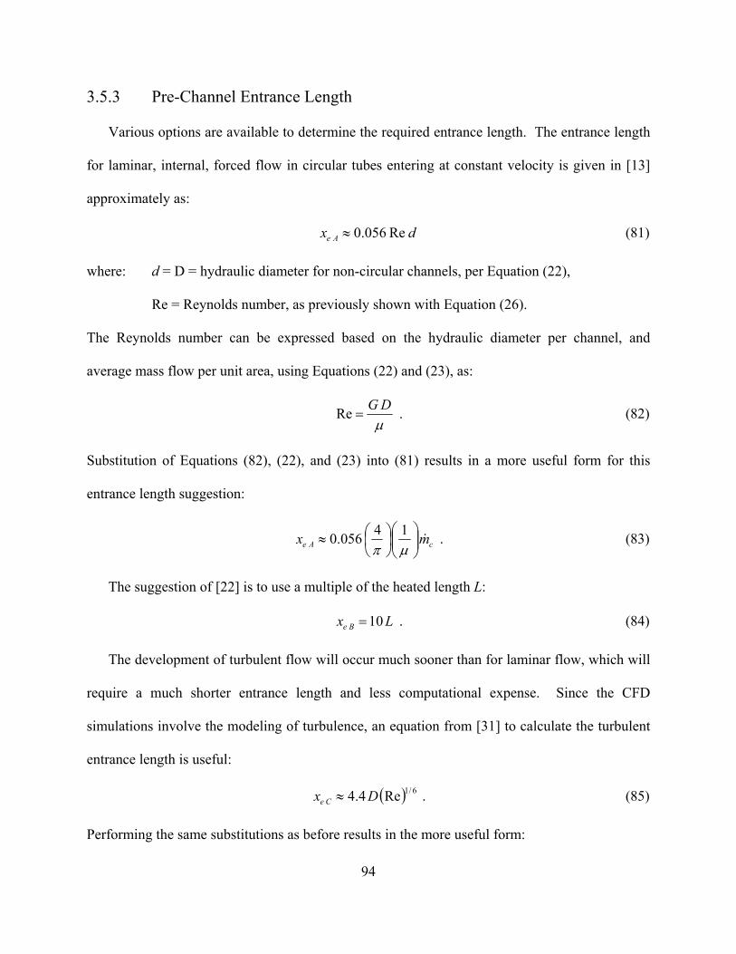
94
3.5.3 Pre-Channel Entrance Length
Various options are available to determine the required entrance length. The entrance length
for laminar, internal, forced flow in circular tubes entering at constant velocity is given in [13]
approximately as:
dx Ae Re056.0 (81)
where: d = D = hydraulic diameter for non-circular channels, per Equation (22),
Re = Reynolds number, as previously shown with Equation (26).
The Reynolds number can be expressed based on the hydraulic diameter per channel, and
average mass flow per unit area, using Equations (22) and (23), as:
DG
Re . (82)
Substitution of Equations (82), (22), and (23) into (81) results in a more useful form for this
entrance length suggestion:
cAe mx
14
056.0 . (83)
The suggestion of [22] is to use a multiple of the heated length L:
Lx Be 10 . (84)
The development of turbulent flow will occur much sooner than for laminar flow, which will
require a much shorter entrance length and less computational expense. Since the CFD
simulations involve the modeling of turbulence, an equation from [31] to calculate the turbulent
entrance length is useful:
6/1Re4.4 Dx Ce . (85)
Performing the same substitutions as before results in the more useful form:

95
6/56/1
2144.4
hw
hwmx cCe . (86)
Each entrance length value should be compared for reasonableness.

96
CHAPTER 4
METHODOLOGY TO DESIGN AND OPTIMIZE REGENERATIVE
COOLING CHANNELS
This chapter presents the methodology required for the design and optimization of
regenerative cooling channels, as performed for the cSETR 50lbf engine. Although CFD
software is used, extensive hand calculations are required beforehand. The design begins with a
preliminary stress analysis to determine a set of design features, then involves a thermal analysis
to determine a set of channel geometries to investigate, and finally the CFD software FLUENT is
used to find the optimal configuration.
4.1 Preliminary Stress Analysis
The design of regenerative cooling channels begins with a preliminary stress analysis. The
purpose of being preliminary is to indicate that only basic theory is involved, and must be
expanded upon in future design iterations for increased structural integrity. The stress analysis
itself is required to formulate specific design features which are necessary for the cooling
performance, as well as to build the regenerative cooling system upon a solid structural
foundation without design excess. Any future work on the design determined through this
preliminary analysis should take the methods and purposes used into consideration.
4.1.1 Analysis of Loading Conditions
Proper structural design must be based on at least the minimum anticipated loading

97
conditions. Only pressure and temperature loads are considered for the preliminary structural
analysis. Other loads are required to be analyzed for a more detailed design, for instance thrust
and mounting.
The combustion chamber pressure for the cSETR 50lbf engine is used as the basis in the
determination of other pressure loads and values. From Table 2-18, pc = 1.5 x 10⁶ N/m2.
Options for the minimum channel outlet pressure are then calculated using Equations (1), (2),
(3), and (4), which depend on the injector design, to give:
a) Equation (1) with (2): 1minoutP = 1,542,861.60645 ≈ 1.54 x 10⁶ N/m2
b) Equation (1) with (3): 2minoutP = 1.8 x 10⁶ N/m2
c) Equation (4): 3minoutP = 3.0 x 10⁶ N/m2
Next, options for the minimum pressure drop in the cooling channel are estimated from various
literature references, since actual drops will be determined in the CFD simulations:
a) from Figure 2-7 for methane: ∆P1 = 600,000 = 0.6 x 10⁶ N/m2
b) from [6] for hydrogen used in an engine larger than the cSETR 50lbf engine:
∆P2 = 5.0 x 10⁶ N/m2
c) from Table 2-9 for methane used in an engine much larger than the cSETR 50lbf
engine: ∆P3 = 1,158,319.2252 ≈ 1.2 x 10⁶ N/m2
An injector pressure drop of one full value of the combustion chamber pressure as used for
3minoutP seems excessive. The injector design values are not known, but a "good" design can be
assumed. The values of 2minoutP and ∆P1 are chosen, which allow the calculation of the cooling
channel minimum allowable inlet pressure from Equation (5) to be mininP = 2.4 x 10⁶ N/m2.
Finally, the effective pressure on the idealized beam located at the bottom of the channel, as per

98
Figure 3-3, is determined with Equation (32) to be peff = 0.9 x 10⁶ N/m2.
Yield pressure and ultimate failure pressure load conditions are found individually for the
inner shell and outer shell. For the inner shell, the working load under normal steady-state
operating conditions is set by the design of the cSETR 50lbf engine as the chamber pressure. For
the outer shell, the working load is the cooling channel minimum allowable inlet pressure.
Equations (44) through (54) are used, with the resulting values shown in Table 4-1.
Table 4-1: Yield and ultimate load conditions for the inner and outer shells.
Equation Inner Shell Value, [N/m2] Outer Shell Value, [N/m2]
(44) LA = pc = 1.5 x 10⁶ LA = Pin min = 2.4 x 10⁶
(45) LB ≈ 1.5 x 10⁶ LB ≈ 2.4 x 10⁶
(46) LC = 1.65 x 10⁶ LC = 2.64 x 10⁶
(47) LD = 1.8375 x 10⁶ LD = 2.94 x 10⁶
(48) LL A = 1.8 x 10⁶ LL A = 2.88 x 10⁶
(49) LL B = 1.8 x 10⁶ LL B = 2.88 x 10⁶
(50) LL C = 1.815 x 10⁶ LL C = 2.904 x 10⁶
(51) LL D = 1.8375 x 10⁶ LL D = 2.94 x 10⁶
(52) LDL = 1.8375 x 10⁶ LDL = 2.94 x 10⁶
(53) LY inner = 2.02125 x 10⁶ LY outer = 3.234 x 10⁶
(54) LU inner = 2.75625 x 10⁶ LU outer = 4.41 x 10⁶
The typical operating temperature ranges found in [16] for the hot-wall and channel lower
wall are used to set an expected thermal load of ∆Texp = (806 - 478) = 328 K between the two
walls, since the actual value will be determined in the CFD simulations. This load occurs for the
inner shell which is typically made of NARloy-Z, thus the maximum temperature differential
allowed before yielding occurs is calculated by Equation (39) using the properties of Table 2-5 to
be ∆Tmax = 71.77 K. The expected temperature differential is greater than this yield value, but a
definite conclusion can not be made because Equation (39) is not a function of the material

99
thickness. A thicker material of certain geometry is expected to withstand the loads, thus the
result warrants the investigation of cyclic stress analysis to determine the geometry.
4.1.2 Chamber Wall Thickness Determination
Recall that when the cooling channels are milled out of the inner shell, a relatively thin
portion remains in the location beneath the channels termed the "chamber wall". As the thinnest
location, the chamber wall thickness is a critical design location and must be able to withstand
the expected loads. This is accomplished with the circumferential stress Equation (31) to
directly determine the thickness. Afterward, design ratios can be determined from literature
values or other equations, for comparison and determination of other cross sectional geometry
features.
From the collection of possibly used inner shell materials, Equation (31) is used with the
radius of the combustion chamber, combustion chamber pressure, and various yield, ultimate, or
endurance loads and material limits from Tables 2-5, 2-6, 2-18, and 4-1 to compile Tables 4-2
for minimal safety factor yield criteria, 4-3 for working loads yield criteria, and 4-4 for working
loads ultimate criteria. The use of the larger combustion chamber radius adds a safety factor into
the design as the results are applied to the smaller radius throat. Typically, endurance strength
values are unknown, but if known they are used rather than the ultimate strength for the chamber
wall which is subject to cyclic loading.

100
Table 4-2: Various calculated chamber wall thicknesses for minimal safety factor yield criteria designs. Equation (31) used with listed input parameters, rcc = 0.01625 m, and pc = 1.5 x 10⁶ N/m2.
Material Strength Criteria,
σY, [N/m2] Thickness, [mm]
NARloy-Z 78.3875 x 10⁶ tmin 1 = 0.311
Copper, Annealed 33.3 x 10⁶ tmin 2 = 0.732
Copper, OFHC Soft 49 or 78 x 106 tmin 3 = 0.497 or 0.313
Copper, OFHC Hard 88 or 324 x 106 tmin 4 = 0.277 or 0.075
Copper, Annealed OFHC 29.915 x 10⁶ tmin 5 = 0.815
Copper, OFHC 1/4 Hard 310 x 106 tmin 6 = 0.079
Copper, OFHC 1/2 Hard 317 x 106 tmin 7 = 0.077
Table 4-3: Various calculated chamber wall thicknesses for working loads yield criteria designs. Equation (31) used with listed input parameters, rcc = 0.01625 m, and LY inner = 2.02125 x 10⁶ N/m2.
Material Strength Criteria,
σY, [N/m2] Thickness, [mm]
NARloy-Z 78.3875 x 10⁶ tmin 8 = 0.419
Copper, Annealed 33.3 x 10⁶ tmin 9 = 0.986
Copper, OFHC Soft 49 or 78 x 106 tmin 10 = 0.67 or 0.421
Copper, OFHC Hard 88 or 324 x 106 tmin 11 = 0.373 or 0.101
Copper, Annealed OFHC 29.915 x 10⁶ tmin 12 = 1.098
Copper, OFHC 1/4 Hard 310 x 106 tmin 13 = 0.106
Copper, OFHC 1/2 Hard 317 x 106 tmin 14 = 0.104

101
Table 4-4: Various calculated chamber wall thicknesses for working loads ultimate or endurance criteria designs. Equation (31) used with listed input parameters, rcc = 0.01625 m, and LU inner = 2.75625 x 10⁶ N/m2.
Material Strength Criteria, σU or σE, [N/m2]
Thickness, [mm]
NARloy-Z 137.9 x 10⁶ (note: σE) tmin 15 = 0.325
Copper, Annealed 210 x 106 tmin 16 = 0.213
Copper, OFHC Soft 215 x 106 tmin 17 = 0.208
Copper, OFHC Hard 261 x 106 tmin 18 = 0.172
Copper, Annealed OFHC 202 x 106 tmin 19 = 0.222
Copper, OFHC 1/4 Hard 330 x 106 tmin 20 = 0.136
Copper, OFHC 1/2 Hard 344 x 106 tmin 21 = 0.130
The thickness results represent the minimum allowable thicknesses for the associated load and
strength values. The worst-case-scenario for the chamber wall thickness is tmin 12 = 1.098 mm.
This value also exceeds the minimum allowable chamber wall thickness reported in [7], [12], and
[16]. Even though the value obtained is not for NARloy-Z, this material is the most likely to be
used for engine construction and its higher strength adds to the safety factor of the design.
With the chamber wall thickness determined, the radius to the outer surface of the chamber
wall (to the bottom of the channel) is found by combining the inner surface throat radius from
Table 2-18 to be ro = 0.006248 m. Because the above stress calculations used the larger chamber
radius, the resulting thicker wall when applied to the throat adds a safety factor to the critical
thermal and stress location of the throat. Had the throat radius been used before, the wall
thickness would have been much less and resulted in a weaker design. The construction of the
engine is likely to be from one piece of material with a constant wall thickness from the nozzle,
to the throat, to the combustion chamber.

102
4.1.3 Outer Shell Thickness Determination
Calculation of the outer shell thickness is performed in a manner similar to that for the
chamber wall, using Equation (31). Because the fin height has not yet been found in the
proceeding thermal analysis, an estimated radius value to the outer shell must be used. Starting
with the chamber radius, the maximum possible fin height is about 8 mm, thus the value to the
outer shell can be rJ = 25.065 mm. For an Inconel 718 outer shell, Tables 2-7 and 4-1 are used to
obtain the minimum permissible thicknesses shown in Table 4-5.
Table 4-5: Various calculated outer shell thicknesses for Inconel 718 subject to different loading conditions. Equation (31) used with listed input parameters and rJ = 25.065 mm.
Pressure Load, [N/m2] Strength Criteria,
[N/m2] Thickness, [mm]
Pin min = 2.4 x 10⁶ σY = 980 x 106 tmin J 1 = 0.0614
LY outer = 3.234 x 10⁶ σY = 980 x 106 tmin J 2 = 0.083
LU outer = 4.41 x 10⁶ σU = 1100 x 106 tmin J 3 = 0.1
The worst-case-scenario for the outer shell thickness is tmin J 3 = 0.1 mm, however due to the
limitations of HyperMesh a value of tJ = 1.0 mm is required, and is realistic.
4.1.4 Channel Width to Chamber Wall Thickness Design Ratio
A set of specific design ratios is required to relate the above calculated chamber wall
thickness to other geometric features of the cooling channel cross section. The first such design
ratio involves the channel width and chamber wall thickness,
t
w, which can be interpreted as
t
w =
max
t
w =
t
wmax =
mint
w for yield or ultimate loads and material strengths.

103
Therefore, the most critical ratio quantity which represents a likely failure design is the largest,
and the ratio which represents a low chance for failure is the smallest.
Various literature references are utilized for the extraction of this ratio from the values they
provide, not necessarily at the throat because a maximum ratio is needed in the determination of
failure probability. A maximum channel width, or minimum chamber wall thickness, provides
the maximum ratio. Tables 2-1, 2-4, and 2-2 are used to formulate this ratio, and the values are
reported in Tables 4-6, 4-7, and 4-8. The values for Table 4-7 from [6] require the calculation of
the chamber wall thickness using Equation (31), the pressure of 11 x 106 N/m2, the assumed
material OFHC 1/4 hard copper in Table 2-6, and chamber radius of 0.06 m, giving t = 2.129
mm.
Table 4-6: Literature values of the channel width to chamber wall thickness ratio, as found from [16] and Table 2-1.
Channel Width,
w, [mm]
Chamber Wall Thickness,
t, [mm] Ratio,
t
w
0.301 7.6 0.0396
0.338 7.6 0.0445
0.335 7.6 0.0441
0.663 7.6 0.0872
0.442 7.6 0.0582
0.373 0.635 0.5874
0.963 7.6 0.1267
0.427 7.6 0.0562
0.564 7.6 0.0742
0.919 7.6 0.1209
1.016 7.6 0.1337
0.411 7.6 0.0541
2.169 7.6 0.2854
0.569 7.6 0.0749
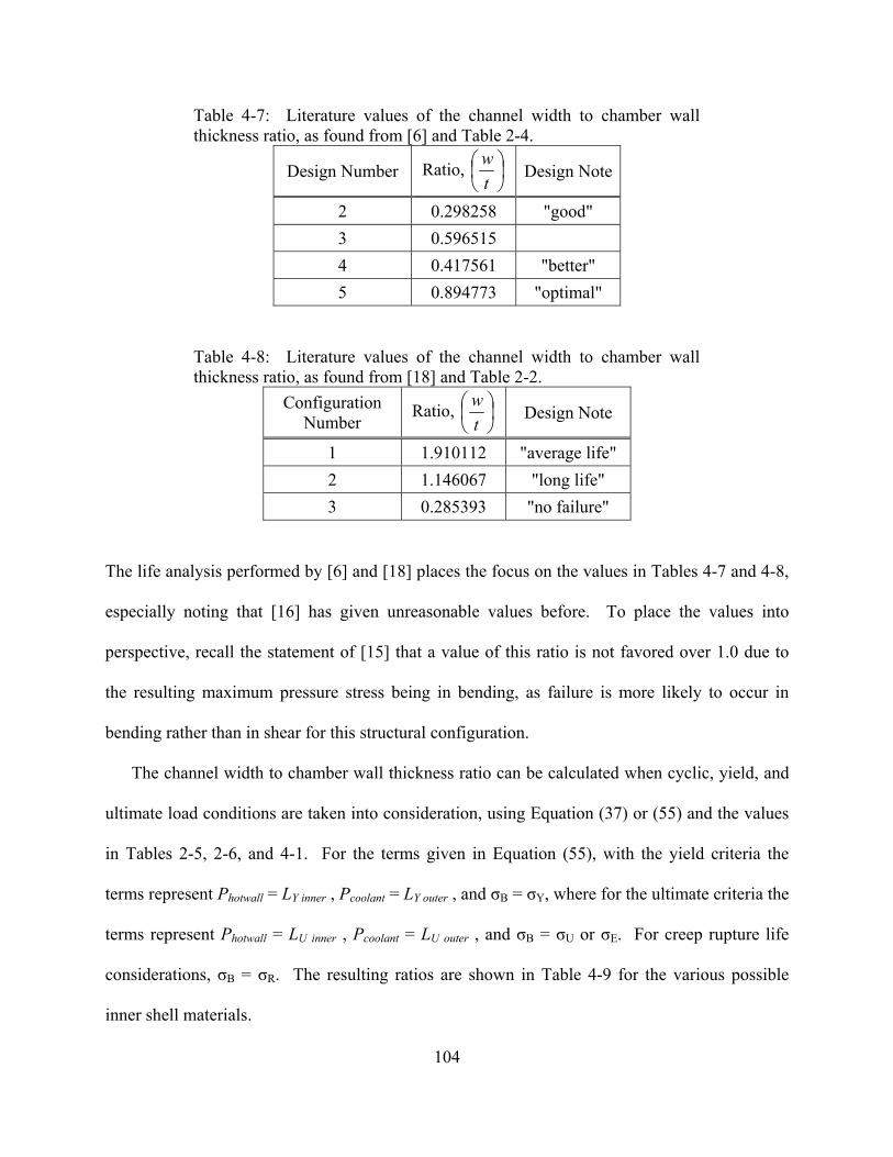
104
Table 4-7: Literature values of the channel width to chamber wall thickness ratio, as found from [6] and Table 2-4.
Design Number Ratio,
t
w Design Note
2 0.298258 "good"
3 0.596515
4 0.417561 "better"
5 0.894773 "optimal"
Table 4-8: Literature values of the channel width to chamber wall thickness ratio, as found from [18] and Table 2-2.
Configuration Number
Ratio,
t
w Design Note
1 1.910112 "average life"
2 1.146067 "long life"
3 0.285393 "no failure"
The life analysis performed by [6] and [18] places the focus on the values in Tables 4-7 and 4-8,
especially noting that [16] has given unreasonable values before. To place the values into
perspective, recall the statement of [15] that a value of this ratio is not favored over 1.0 due to
the resulting maximum pressure stress being in bending, as failure is more likely to occur in
bending rather than in shear for this structural configuration.
The channel width to chamber wall thickness ratio can be calculated when cyclic, yield, and
ultimate load conditions are taken into consideration, using Equation (37) or (55) and the values
in Tables 2-5, 2-6, and 4-1. For the terms given in Equation (55), with the yield criteria the
terms represent Photwall = LY inner , Pcoolant = LY outer , and σB = σY, where for the ultimate criteria the
terms represent Photwall = LU inner , Pcoolant = LU outer , and σB = σU or σE. For creep rupture life
considerations, σB = σR. The resulting ratios are shown in Table 4-9 for the various possible
inner shell materials.

105
Table 4-9: Values of the channel width to chamber wall thickness ratio for various inner shell materials, as found from Equation (55).
Material Yield, Yt
w
Ultimate,
Ut
w
Rupture,
Rt
w
NARloy-Z 11.369798 12.914042
yield loads: 5.840493
ultimate loads: 5.001499
Copper, Annealed 7.410568 15.936381
Copper, OFHC Soft 8.989331 or 11.341661
16.124984
Copper, OFHC Hard 12.046772 or
23.115424 17.766436
Copper, Annealed OFHC 7.023828 15.629884
Copper, OFHC 1/4 Hard 22.610502 19.977311
Copper, OFHC 1/2 Hard 22.864357 20.396671
Because material failure considerations were taken into account for determining the values in
Table 4-9, the values are maximums placed on this ratio. The absolute maximum is maxabs
t
w =
5.001499, thus no actually used geometries should exceed this value. If the ratio used is well
below the maximum, cyclic failure is not extremely likely within a reasonable engine life.
Taking the advice of [15], the optimal ratio
t
w = 0.894773 from [6] is justified for determining
the maximum channel width for a constant chamber wall thickness. Also, the smallest "no
failure" ratio of Table 4-8,
t
w = 0.285393, is used to determine the minimum width for a
constant thickness.

106
4.1.5 Fin Width to Channel Width Design Ratio
The next required design ratio links the previously determined design features to a new
quantity. The fin width to channel width ratio,
w
f , can be interpreted as
w
f = max
w
f =
w
f max =
minwf if necessary to correspond to the previously determined channel width, but is
usually not a fixed quantity because the fin width can be varied along the engine length to
accommodate the varying circumference for a designed channel width. Therefore, only the ratio
at the thermally critical throat location is necessary for definition, and the ratio can be adjusted at
a later time for the other engine locations in consideration of channel pressure drop.
Various literature references are utilized for the extraction of this ratio from the values they
provide. Table 2-4 and [12] are used, and the values are reported in Table 4-10.
Table 4-10: Literature values of the fin width to channel width ratio, as found from [12] and Table 2-4.
Design Number Ratio,
w
f Design Note
1 and 3 7.4 or 2.7
2 1.1 "good"
4 1.1 "better"
5 1.1 "optimal"
none, [12] 1.0
No options are available for calculating this ratio in the literature for the critical throat
location, therefore the most commonly used
w
f = 1.1 is chosen due to its use in all of the
noted best designs of Table 4-10 and fitting into the negligible influence range given by [15].

107
4.1.6 Fin Height to Fin Width Design Ratio
The next design ratio to be considered again links the previously determined design features
to a new quantity. The fin height to fin width ratio,
f
finL
, can be interpreted as
f
finL
=
max
f
finL
=
f
finL
max =
minf
finL
as for previous ratios, but is more useful as a comparison tool.
Various literature references are utilized for the extraction of this ratio from the values they
provide, however only [6] is useful as [16] does not give the required inputs directly. Table 2-4
is used, and the values are reported in Table 4-11.
Table 4-11: Literature values of the fin height to fin width ratio, as found from Table 2-4.
Design Number Ratio,
f
finL
Design
Note
1 and 3 5.405 or 2.852
2 4.545 "good"
4 4.545 "better"
5 4.545 "optimal"
The fin height to fin width ratio is also calculated when column buckling possibilities are
taken into consideration, using Equation (43) and Table 2-5 for NARloy-Z. Calculating the ratio
gives
min
max
f
finL
= 527.771, which upon comparison to the values in Table 4-11 suggests that
buckling in this manner is not a concern. Furthermore, the fin height will later be calculated
directly based on optimized heat transfer into the coolant.

108
4.1.7 Summary of Important Values for Later Use
The values presented in Table 4-12 are compiled based on the results of the literature review
and the preliminary stress analysis, and are required for additional calculations. The pressure
values are also used for comparison to the CFD results of the present research.
Table 4-12: Summary of important values to be used in the present research for subsequent calculations and comparison.
Property Description Value Channel Width Minimum
Fabrication Limit w ≥ 0.5 mm
Channel Height Maximum Fabrication Limit
h ≤ 8 mm
Inner Shell Material NARloy-Z
Outer Shell Material INCONEL 718
Minimum Allowable Cooling Channel Outlet Pressure 2minoutP = 1.8 x 10⁶ N/m2
Minimum Allowable Cooling Channel Inlet Pressure mininP = 2.4 x 10⁶ N/m2
Minimum Combustion Chamber Wall Thickness
tmin 12 = 1.098 mm
Radius of Throat on Outer Surface
ro = 0.006248 m
Outer Shell Thickness tJ = 1.0 mm
Channel Width to Chamber Wall Thickness Design Ratio, For
Maximum w
t
wmax = 0.894773
Channel Width to Chamber Wall Thickness Design Ratio, For
Minimum w
t
wmin = 0.285393
Fin Width to Channel Width Design Ratio
w
f = 1.1

109
4.2 Thermal Analysis
The design of regenerative cooling channels next involves a thermal analysis to determine a
set of channel geometries to investigate in the subsequent CFD simulations. With the design
features obtained through the preliminary stress analysis, the thermal analysis can proceed by
applying the theories of heat transfer to the combustion chamber, cooling fins and channels, and
outer shell.
The effects of the wall contour and channel curvature on the coolant flow characteristics are
not studied in the present research, since they can be studied separately from the thermal effects.
Instead, the Bartz equation is utilized to provide the curvature induced heat transfer coefficient
variation along the hot-wall, but with straight channels. The curvature may have an effect on the
cooling performance, therefore this method provides an initial set of results to which the
curvature effects can be added for future research.
4.2.1 Combustion Chamber Thermal Conditions
The thermal analysis of a rocket engine begins with the combustion of the fuel and oxidizer,
which is the source of the heat which must be extracted by the regenerative cooling system.
Knowledge of the combustion temperature is necessary to then find the amount of heat that is
transferred to the hot-wall surface and into the chamber wall of the inner shell. From the
chamber wall, the heat is then transferred to the cooling channels via the channel lower wall, or
into the fins and then into the channel via the fin walls adjacent to the coolant.

110
4.2.1.1 adiabatic flame temperature of combustion
The combustion temperature is determined through a calculation of the adiabatic flame
temperature of the combusting gasses, comprised of oxygen and methane (O2/CH4), subject to
the following assumptions. Adiabatic combustion at constant enthalpy for an ideal gas mixture
is assumed, which itself assumes complete combustion although an incomplete combustion
process must be considered due to the mixture ratio balance requirements of Equation (56).
Also, the reactants begin at the steady state injection temperature of methane, equivalent to the
temperature at the channel outlet per Table 2-9, of Ti = 526.222 K. This value is assumed since
the actual value will be determined in the CFD simulations. The pressure dependence on the
reaction is unknown, H2O stays gaseous, and component properties are determined from Tables
2-12 and 3-1.
It is assumed that the given mixture ratio of Table 2-18 is on a mass basis because of the m
ratio equivalence, thus it must be converted to a molar basis:
4
2
2
2
4
4
4
2
CHkmol
Okmol16013520970.1
Okg31.998
Okmol1
CHkmol1
CHkg0426.16
CHkg0.018
Okg0575.0
molarMR
The incomplete combustion reaction, Equation (56), is subject to the following conditions in
order to balance properly:
1) to balance based on mixture ratio: a
b = 1.60135209701
2) to balance carbon: a = c + e
3) to balance hydrogen: a = (1/2) d
4) to balance oxygen: b = c + (1/2) d + (1/2) e
Equation (58) is for per mole of fuel, so the coefficient a = 1. When balanced, the following
molar coefficients are discovered:

111
a) reactants:
1) nCH4 R = 1 kmol
2) nO2 R = 1.60135209701 kmol
b) products:
1) nCO2 P = 0.20270419402 kmol
2) nH2O P = 2 kmol
3) nCO P = 0.79729580598 kmol
Because h °f of Table 2-12 is given for the standard condition temperature T° = 298.15 K,
and since the reactants begin at the assumed injection temperature of Ti = 526.222 K, the
reactants must be "cooled" down to T° before the reaction, then allowed to react from T° up to
the adiabatic flame temperature desired, Tad. When Equation (59) is substituted into Equation
(58), the heat equation becomes:
PCO2PCO2RO2RO2RCH4RCH4 hhnhhnhhn fff
PCOPCOPH2OPH2O hhnhhn ff
.
Next, using Equation (60) gives:
dTTcnTcnhnhn ppff
15.298
222.526 O2RO2CH4RCH4RO2RO2RCH4RCH4
PCOPCOPH2OPH2OPCO2PCO2 fff hnhnhn
dTTcnTcnTcnadT
ppp 15.298 COPCOH2OPH2OCO2PCO2 .
This equation is solved for Tad using the symbolic mathematics solver program MAPLE, giving
Tad = 4,269.158187 K as shown in Appendix I. Comparing this value to the lower values from

112
Table 2-18, [10], and [15], indicates that any subsequent calculations using this flame
temperature will result in a desirable over-design as it adds an inherent safety factor to the
cooling system.
4.2.1.2 parameters needed for the Bartz equation
Certain parameters and terms in the Bartz equation of Equations (10) and (11) require
preliminary definition. First, the hot-wall temperature, Twh, is unknown directly as that value is
to be determined in the CFD simulations and is controlled by the cooling system performance.
An assumed average reference value from literature is used to obtain an initial heat transfer
coefficient, then if desired the value found from the later CFD results can be used in an iterative
approach in future research. The value from [16] is chosen, Twh = 806 K.
Next, the temperature ratio found in the correction factor of Equation (11) is defined using
the adiabatic flame temperature determined previously:
188796.0158187.4269
806
0
nsc
wg
g
wh
T
T
T
T ,
which falls between the (1/8) and (1/4) curves in Figure 2-5. The last item needed in order to
find the correction factor placement is the specific heat ratio of Equation (12), using the
reaction coefficients determined previously and the values from [31]:
RO2RCH4
RO2RO2CH4RCH4
nn
nn
n
n
ii
iii
avgmixture
358.1
601.2
395.1601.1299.11
,

113
which falls between the 1.3 and 1.4 curves. A linear interpolation using Equation (13) is used to
determine the proper correction factor values between the bounding temperature and specific
heat curves. Then, the Prandtl number of Equation (14) is Pr = 0.752146219884.
The dynamic viscosity is calculated using Equation (15) with proper unit conversion. To
begin, the molecular weight of the combustion products is found using Table 2-12:
kmol
kg0338.9001.280148.18009.44COH2OCO2 MWMWMWMW ,
converted to:
mol
lbm111984905522.0
mol1000
kmol1
kg0.45359237
lbm1
kmol
kg0338.90MW .
The temperature used is the adiabatic flame temperature, converted:
R4847366.7684K158187.4269 adTT .
Therefore, the dynamic viscosity becomes 0 = 4.45 x 10⁻⁷ [lb/in-sec], and when converted back
to the required units:
sm
kg1049516400416.7
m1054.2
in1
lbm1
kg45359237.0
secin
lb1045.4 5
37
0 .
The specific gas constant of the combustion gas products is calculated from Equation (17)
and converted to:
Kkg
J3430978144.92
kJ1
J1000
kg
kmol
Kkmol
kJ
0338.90
314.8R ,
so that the combustion gas specific heat of Equation (16) is cp0 = 350.284711821 [J/kg-K].
The local cross sectional area is found graphically from Figure 1-10.

114
4.2.1.3 Bartz heat transfer coefficient variation
The heat transfer coefficient variation along the hot-wall is determined along the true channel
length from Table 2-18, using the local cross sectional area variation from Figure 1-10, the
correction factor variation from Figure 2-5, the Bartz Equation of Equation (10), and a
numerically based spreadsheet software. The result, shown in Appendix II, compares well to
literature examples when graphed in Figure 4-1, with the nozzle exit at the far left, the expected
peak at the throat, and the injector at the far right. For comparison, the variation along the true
"flattened" channel length (not axially projected) is shown with the variation along the axially
projected length. The true length is needed for a CFD simulation using a straight channel with
no curvature.
0
200
400
600
800
1000
1200
1400
1600
0 20 40 60 80 100 120 140 160
length, [mm]
h g ,
[W/m
2-K
] true length
axial length
Figure 4-1: Heat transfer coefficient variation of Bartz along the cSETR 50lbf engine hot-wall versus length along hot-wall. The left portion is in the engine nozzle, the peak indicates the throat, and the right portion is in the combustion chamber. Values correspond to Appendix II.

115
4.2.2 Fin and Cooling Channel Thermal Conditions
The thermal analysis of the fin and cooling channel determines the geometries which provide
optimal heat transfer from the solid fin to the fluid coolant, beginning with a determination of the
fin height. Multiple geometries are possible due to the circumferential allowance for different
numbers of channels, nc, each geometry providing the optimal heat transfer for the particular nc.
4.2.2.1 fin height and heat transfer coefficients
The extended surface cooling fin equation of Equation (20) is used to determine the fin
height which provides the optimal heat transfer, subject to fabrication constraints. Combining
the fin width to channel width design ratio of Table 4-12 and the circumferential length
relationship of Equation (25) gives the following allowance for the fin width in terms of the
number of channels and outer throat radius:
c
of n
r21
22 .
Substituting this term into the fin height equation, rearrangement, and application to multiple
inputs of the heat transfer coefficient gives:
c
oig
c
foi n
r
n
rh
21
11
21
114192.1 5.0
5.0
,
where the subscript i indicates the pairing.
Equation (25) and the ratio of Table 4-12 are also rearranged to give the channel width
allowance:
c
o
n
rw
1.2
2 .

116
Using this term with the bulk mean temperature as the standard state condition temperature, and
Equations (22), (23), and (24), allows the first heat transfer coefficient of Equation (21) to be
rearranged into the form:
8.18.0
1 05.1
2A
hnr
hr
n
m
co
o
c
tg
,
which contains the fin height, and where the constants have been grouped into:
67.047.033.08.0
40.023A bbpc
.
Similarly by following [28], the other heat transfer coefficients of Equations (26), (27), and (28)
become:
8.1
8.02 05.1
2B
hnr
hrn
co
ocg
,
with
8.014.04.026.06.08.0
40.023B twpbb mc
;
and,
8.1
8.03 05.1
2D
hnr
hrn
co
ocg
,
with
8.014.03/1150/493/28.0
40.027D twpbb mc
;
and,

117
8.1
8.04 05.1
2E
hnr
hrn
co
ocg
,
with
8.0
55.0
3/115/73/28.0
40.029E t
wc
copbb m
T
Tc
.
This rearrangement shows that all of the equations are basically the same, differing only by the
constant terms.
4.2.2.2 parameters needed for coolant side heat transfer
Certain parameters and terms require preliminary definition for the subsequent fin height and
coolant side heat transfer calculations. For coolant bulk temperature requests, as the quantity is
unknown before the CFD simulations, the standard reference temperature of Tco = 298.15 K is
chosen. Also unknown beforehand is the cooling channel lower wall temperature, thus per [16]
the value used is Twc = 533 K.
Setting the cooling channel lower wall temperature allows the calculation of the coolant
viscosity at that wall temperature, w , using Sutherland's Equation of Equation (29) and the
bounding viscosity values from Table 2-11. The constants become:
a) C2 = 1.01567799509 x 10⁻⁶ kg/m-s-K1/2
b) S = 180.182597411 K
Thus, at Twc = 533 K, w = 1.7525 x 10⁻⁵ kg/m-s.
Equation (25) and the ratio of Table 4-12 are again rearranged to give the number of channels
possible for the outer throat radius and some channel width:

118
w
rn o
c 1.2
2 .
The minimum number of cooling channels possible is stress limited and found using this
relationship, the maximum width ratio, and other values from Table 4-12. The maximum width
calculates to wmax = 0.000982 m, and the minimum number of channels is rounded to the whole
number of nc min = 19.
The maximum number of cooling channels possible is fabrication limited and found using
the above relationship, the minimum width ratio, and other values from Table 4-12. The
minimum width possible calculates to wmin = 0.0003 m, which is below the fabrication limits of
[3] so a value of wmin = 0.0005 m must be used. The maximum number of channels is thus nc max
= 37.
4.2.2.3 iteration of fin height equation
With the heat transfer coefficient equations containing the fin height as a variable, and the fin
height equation containing the heat transfer coefficient as a variable, the equation for the fin
height must be iterated to find the optimal value. The option of four heat transfer coefficient
equations increases the complexity. A numerical iteration algorithm, shown in Appendix III, is
written in the MATLAB programming language with the above equations, constants, and
relationships to perform the required computations. The algorithm handless divergence as it
takes each of the four heat transfer coefficient equations and pairs them one at a time with the fin
height equation, resulting in four heights to choose from. This is done for each of the possible
number of channels, nc from 19 to 37, resulting in an additional selection of fin heights.
The results of the iterations, given in Appendix IV, show that each heat transfer equation

119
gives similar coefficient and height values. The choice of which to use is not clear, so an
average is taken to provide only the nineteen heights associated with the possible nc. Only two
nc with the maximum height of 8 mm is used, reducing nc to the range from 22 to 37. By using
the nomenclature that nc = 22 represents the geometry needed for the case of 22 total channels
placed about the engine circumference, and so on for all nc, then only sixteen CFD channel
models are needed in total and are represented by nc = 22 to nc = 37.
The channel cross sectional details of Figures 4-2 through 4-5, some resulting from the
averaging, are used for the CFD models.
0.0055
0.0060
0.0065
0.0070
0.0075
0.0080
22 23 24 25 26 27 28 29 30 31 32 33 34 35 36 37
Number of Channels, nc
Ch
ann
el H
eig
ht,
[m
]
Figure 4-2: Geometry variation for the channel models nc of channel height. Values correspond to Appendix IV.

120
2.5E-04
2.7E-04
2.9E-04
3.1E-04
3.3E-04
3.5E-04
3.7E-04
3.9E-04
4.1E-04
4.3E-04
22 23 24 25 26 27 28 29 30 31 32 33 34 35 36 37
Number of Channels, nc
Ch
ann
el H
alf
Wid
th,
[m]
Figure 4-3: Geometry variation for the channel models nc of the CFD modeled channel half widths. Values correspond to Appendix IV.
9.40
9.60
9.80
10.00
10.20
10.40
10.60
10.80
11.00
22 23 24 25 26 27 28 29 30 31 32 33 34 35 36 37
Number of Channels, nc
Ch
ann
el A
R
Figure 4-4: Geometry variation for the channel models nc of the channel aspect ratio using the channel height and full width. Values correspond to Appendix IV.

121
4.50E-04
5.00E-04
5.50E-04
6.00E-04
6.50E-04
7.00E-04
7.50E-04
8.00E-04
8.50E-04
22 23 24 25 26 27 28 29 30 31 32 33 34 35 36 37
Number of Channels, nc
Ch
ann
el M
ass
Flo
w R
ate,
[kg
/s]
Figure 4-5: Flow variation for the channel models nc of the channel mass flow rate. Values correspond to Appendix IV.
4.2.3 Outer Shell Thermal Conditions
Two boundary condition options are used for the outer shell thermal conditions. The first is
convection to atmosphere. The properties of air from Table 2-17, a relatively stagnate condition
of wm = 1.0 m/s, and Equation (30) are used to give the mean heat transfer coefficient on the
outer surface of m = 15.592445 W/m2-K.
The second option is radiation to vacuum. The emissivity of rough surfaced nickel from [29]
is used, with an exterior radiation sink temperature assumed to be T = 1 K for Equation (9) so
that the vacuum of space is not at absolute zero. To compare, the average temperature on the
Moon is about 20 K.

122
4.3 Pre-Channel Flow Calculations
As previously explained, in an experimental or CFD model, a pre-inlet entrance length is
added upstream of the inlet to the actual channel section of interest. Flow calculations are
performed to determine the upstream entrance length, using Equations (83), (84), and (86) with
the geometries of Appendix IV. These equations give either unreasonably long or short entrance
lengths, though the turbulent Equation (86) is likely to be at the more accurate end of the
spectrum. Therefore, a middle value of one full channel length is added to the inlet, so that in the
CFD models the CFD channel inlet represents the inlet to the coolant feedline. The inlet to the
portion of the channel which represents the regenerative cooling channel is at the location
downstream (now half way) where heat addition begins, and is termed the modeled-inlet since it
does not represent an actual CFD inlet. In coordinates, using Table 2-18, the CFD inlet is at x =
-0.1562488, the modeled inlet is at x = 0.0, and the cooling channel outlet is at x = 0.1562488.
4.4 CFD Setup Parameters
Several steps are necessary to organize the geometries of Appendix IV and prepare them for
use in the subsequent CFD models.
4.4.1 Geometry Organization
The geometries in Appendix IV require organization in order to be applied to a CFD model,
mainly to define CFD model geometry coordinates. The fin height is equivalent to the channel
height, and because of symmetry only half of the fin width and half of the channel width need to
be modeled in the cross section. The representation shown in Figure 4-6 shows the locations of

123
the points which are organized by nc in Appendix V.
Figure 4-6: Representation of the CFD modeled geometry with drawing coordinate locations indicated. Points associated with Appendix V.
4.4.2 Initial Mesh Determination
The initial mesh for the fluid portion of the geometry is determined using Equation (68) for
the dimensional distance for the first mesh element center, for only the nc = 22 and nc = 37
channel geometries from Appendix IV, using Tables 2-17 and 2-18, and y+min = 30. This mesh
will be refined in the subsequent mesh refinement study.
For nc = 22, w = 0.00085 m, h = 0.008 m, and Equation (68) gives 22minpy = 2.2177 x 10⁻⁵
m. For nc = 37, w = 0.000505 m, h = 0.0055122 m, and Equation (68) gives 37minpy = 1.352

124
x 10-5 m. The associated maximum permissible mesh elements in the vertical and horizontal
directions, for a non-biased rectangular mesh, are given by Equations (69) and (70) as Vmax 22 =
181, Hmax 22 = 20, Vmax 37 = 204, and Hmax 37 = 19. The horizontal number represents the full
channel width. As nc increases, y+ increases to above y+min for the vertical direction, allowing the
use of Vmax 22 as an absolute vertical maximum number of elements for all nc. The widths don't
change as dramatically as the heights for varying nc, and since they are so close, Hmax 22 is also
used.
For the lengthwise mesh, the discretization of the engine geometry and the Bartz heat transfer
coefficient used a ∆x = 0.1 mm, thus for the total channel length of LT = 312.4976 mm, Equation
(71) gives L = 3215 elements ideally. This value may lead to excessive computational times at
little added benefit from a smaller value, and is limited by the CFD software license total cell
limit. The channel cross section mesh is favored, and the lengthwise mesh is reduced to 1000 or
less.
4.4.3 HyperMesh Geometry Generation
The geometries for each nc of Appendix V are placed into separate HyperMesh geometry and
mesh generation files, and the overall significant figures are reduced to a maximum of four. The
mesh information is listed in a later section. The particularly important zones are defined in
Figure 4-7. The very small angles associated with the radial placement of fins and channels
about a circumference are not modeled due to insufficient solution sensitivity information from
[3], [5], [7], and [18]. Four representative examples of the resulting HyperMesh geometries are
shown in Figures 4-8, 4-9, 4-10, and 4-11.

125
Figure 4-7: 2D wall zones, channel inlets and outlet, and 3D regions.
Figure 4-8: Isometric view of entire representative channel.

126
Figure 4-9: Modeled-inlet area showing the solid domains for a representative channel.
Figure 4-10: Alternate view of modeled-inlet area for a representative channel.

127
Figure 4-11: View of inlet of a representative channel showing solid domains, mesh, and half channel and fin widths. Symmetry planes are on both the left and right sides.

128
4.4.4 FLUENT Setup Parameters
The final step before running the CFD simulations is to setup the FLUENT models. Bartz
heat transfer coefficient boundary condition input files, turbulence calculations, and case options
need to be set.
4.4.4.1 boundary condition input files
The variation in the Bartz heat transfer coefficient on the hot-wall, as seen in Figure 4-1, is
taken in its numerically discretized form along the true length and set into a numerical x-y-z
coordinate grid which corresponds to each nc channel individually since the widths are all
different. The grid is located on the hot-wall, and is where the hot-wall is modeled in the
HyperMesh files. The sixteen resulting mesh profile data files are loaded individually into the
corresponding FLUENT case file. The Bartz heat transfer coefficient can then be used as a wall
thermal boundary condition.
4.4.4.2 turbulence model parameters
The turbulence parameters are calculated for the CFD flow inlet, and applied in FLUENT as
turbulence boundary conditions. Using a 2% turbulence intensity, geometry from Appendix IV,
methane properties from Tables 2-12 and 2-18, setting the turbopump exit temperature as the
value for the feedline entrance and CFD flow inlet from Table 2-9, and Equations (73), (74),
(78), (79), and (80), the values for nc = 22 are calculated as:
a) pinlet = 2,461,538.46154 N/m2
b) ρ = 40.233233 kg/m3

129
c) k = 0.07213 m2/s2
d) l = 1.07570621469 x 10⁻⁴ m
e) ε = 29.591453 m2/s3
These values compare well with [46], while the larger values for nc = 37 don't.
4.4.4.3 FLUENT case options and parameters
The options and parameters used in the FLUENT case files for the present research are listed
in Tables 4-13 through 4-21. The 2D walls separating the 3D fluid and solid zones are set as
coupled interface wall zones to allow heat interaction. Smooth surface channel walls are used
with no roughness effects included, and no carbon deposits on any surface.
Table 4-13: FLUENT models prescribed.
Model Property Value
Solver dimension 3D
precision double
solver type pressure based
time formulation steady
velocity formulation absolute
solver formulation implicit
Energy energy equation activated
Viscous model 1 k-epsilon 2 equation
model 2 Reynolds Stress 7 equation
Gas ideal methane Operating Condition
operating pressure 0 pa

130
Table 4-14: FLUENT viscosity model parameters prescribed. Model Property Value
k-ε type realizable
constants default
near wall treatment / wall handling standard wall functions
viscous heating / dissipation activated
RSM type linear-pressure strain
constants default
near wall treatment / wall handling standard wall functions
viscous heating / dissipation activated
wall bc from k equation activated
wall reflection effects activated
Table 4-15: FLUENT domain values prescribed. Domain Material Property Value
Fluid methane density, [kg/m3] ideal gas
Cp, [j/kg-k] piecewise-polynomial
thermal conductivity,
[w/m-k] 0.0332, constant
viscosity, [kg/m-s] 1.087e-05, constant
Solid, Inner Shell
user defined from copper, NARloy-Z
density, [kg/m3] 9134
Cp, [j/kg-k] 373
thermal conductivity,
[w/m-k] 295
Solid, Outer Shell
user defined from nickel, Inconel 718
density, [kg/m3] 8190
Cp, [j/kg-k] 435
thermal conductivity,
[w/m-k] 11.4

131
Table 4-16: Bottom-wall-bottom (hot-wall) FLUENT wall zone boundary conditions.
Property Value
material narloy-z
thermal condition convection
heat transfer coefficient, [w/m2-k] loaded Bartz profile file
free stream temperature, [k] 4269.158187
Table 4-17: Inlet FLUENT mass flow inlet zone boundary conditions. Property Value
mass flow rate, [kg/s] nc dependent per Appendix IV
supersonic/initial gauge pressure, [pa] 2461538.46154
turbulent kinetic energy, [m2/s2] 0.07213
turbulent dissipation rate, [m2/s3] 29.591453
total (stagnation) temperature, [k] 118.055555
Table 4-18: Outlet FLUENT pressure outlet zone boundary conditions. Property Value
gauge (static) pressure, [pa] 1.8e+06
turbulent kinetic energy, [m2/s2] 0.07213
turbulent dissipation rate, [m2/s3] 29.591453
backflow total (stagnation) temperature, [k] 118.055555
Table 4-19: Top-wall-top FLUENT wall zone boundary conditions.
Property Value
material inconel718
thermal condition 1 convection
heat transfer coefficient, [w/m2-k] 15.592445
free stream temperature, [k] 298.15
thermal condition 2 radiation
external emissivity 0.41
external radiation temperature, [k] 1

132
Table 4-20: Various other FLUENT boundary conditions. Zone Type Property Value
multiple 2D adiabatic entrance
wall heat flux, [w/m2] 0
left and right side walls and right side channel
symmetry
multiple external 2D wall heat flux, [w/m2] 0
multiple internal 2D interface
Table 4-21: FLUENT solution monitors, methods and controls.
Parameter Property Value for Iterations 1 to 100
Value for Iterations 101 to
Convergence
Residual Monitors Absolute Criteria 1e-06 for k-ε 1e-06 for k-ε
1e-04 for RSM 1e-04 for RSM Pressure-Velocity Coupling Method
Coupled
Spatial Discretization Methods
Gradient Least Squares
Cell Based Least Squares
Cell Based Pressure Second Order Second Order
Density First Order
Upwind QUICK
Momentum First Order
Upwind QUICK
Turbulent Kinetic
Energy First Order QUICK
Turbulent
Dissipation Rate First Order QUICK
Reynolds Stress
(RSM only) First Order
Upwind QUICK
Energy First Order
Upwind QUICK
Solution Controls, k-ε Courant Number 20 to 30, 100 20 to 30, 100 Solution Controls,
RSM Courant Number 50 50
Solution Controls, both Relaxation Factors default default
Equations Flow, Turbulence, Energy, Reynolds
Stresses (RSM only)

133
4.5 Running the CFD Simulations
The solution behavior and residuals are monitored as the simulations are running to properly
utilize the CFD software and ensure that the results are accurate.
4.5.1 General Simulation Running Techniques and Behavior
The simulations are performed in groups depending on the parameters used:
a) mesh & turbulence sensitivity study, channel nc = 22:
1) k-ε group, 6 meshes, convection outer shell
2) RSM group, 6 meshes, convection outer shell
b) main study with chosen mesh and turbulence model, channels nc = 22 through 37:
1) convection outer shell
2) radiation outer shell
Each simulation, 44 in total, is set to run for 100 iterations with the low order discretizations
shown in Table 4-21. The discretizations are changed to higher order, then the simulations are
continued until convergence.
Convergence is achieved when the equation residuals continue to smoothly decrease for each
successive iteration, and reach the criteria shown in Table 4-21, at which point the simulations
automatically end. In the process of iterating, when FLUENT reports AMG Solver issues and
the solution diverges to the point of automatically ending or stalling, the simulations are stopped
and the Courant number is adjusted. For the mesh & turbulence sensitivity study, a Courant
number of 100 is permitted, though for the main study values of 30 or down to 20 are required.
The initial iterations still report AMG Solver problems, but with the lower Courant numbers,
FLUENT automatically handles the issue and the simulations continue with fewer or no

134
problems until convergence. Convergence is found in under 400 iterations, and is achieved in
under one hour while running on a quad-core desktop PC in a 3 processor parallel mode.
4.5.2 Mesh & Turbulence Sensitivity Study
The simulations performed for the mesh & turbulence sensitivity study use one channel
geometry and the fluid domain mesh densities of Table 4-22. Decreasing the mesh density from
the calculated density has the effect of increasing the y+ value of the wall adjacent cell, which
does not violate the y+ criteria. Domains are matched to the adjoining domain mesh so there is
no boundary discontinuity. The lengthwise mesh covers the total channel length of LT =
312.4976 mm.
Table 4-22: Mesh & turbulence sensitivity study fluid domain mesh densities.
Model Vertical (z)Half Width
Horizontal (y) Lengthwise (x)
nc22_-6 50 4 100
nc22_-5 75 4 150
nc22_-4 100 4 200
nc22_-3 125 4 250
nc22_-2 150 6 350
nc22_-1 125 8 400 nc22_0, as calculated, exceeds total cell limit
so not used 181 10 1000
The determination of the adequate mesh is done graphically by superimposing plots of line
rake solution data for all the mesh density models to see which plot is different. The adequate
mesh is the one with the lowest density and consistent results. The determination of the proper
turbulence model is easier since the RSM plots do not show smooth curves like those of the k-ε

135
plots, instead they wiggle. In the plots, it is seen that the solid portions could probably use a
higher density, but that is not allowed due to the software cell limitations. The thinness of the
channels dictates that the horizontal mesh density is more sensitive to adjustment and should be
kept as high as possible.
4.5.3 Main Study
The mesh and turbulence model chosen from the mesh & turbulence sensitivity study for use
in the main study of channel models nc = 22 to 37 are:
a) fluid domain, V x H x L: 125 X 8 X 380
b) solid domain: matched at edges; as dense as allowed by software cell limitations
c) turbulence model: k-ε
With these values used to setup HyperMesh and Fluent case files, the simulations are performed
and the results of the main study are given in the next chapter. The initialization is performed at
the inlet, giving the values shown in Figures 4-12 and 4-13. Recall that the focus of the current
research is on the cooling performance and selection of the proper nc geometry and configuration
for use with the cSETR 50lbf engine.

136
5.86.06.26.46.66.87.07.27.47.67.88.08.28.48.68.8
22 23 24 25 26 27 28 29 30 31 32 33 34 35 36 37Number of Channels, nc
Vel
oci
ty [
m/s
]
Figure 4-12: Main study initialized x velocity variation for the channel models nc for both convection and radiation boundary types.
118.035
118.040
118.045
118.050
22 23 24 25 26 27 28 29 30 31 32 33 34 35 36 37Number of Channels, nc
Tem
per
atu
re [
K]
Figure 4-13: Main study initialized temperature variation for the channel models nc for both convection and radiation boundary types.

137
CHAPTER 5
RESULTS OF THE MAIN STUDY CFD OPTIMIZATION SIMULATIONS
This chapter presents the results of the CFD simulations used for the determination of the
optimal regenerative cooling system design configuration for the cSETR 50lbf engine. Four
representations are provided: one for general performance characteristics, the second for
performance between nc, the third for performance between geometry, and the forth provides a
real gas assessment. An analysis and discussion are also given of the results as they relate to
material limits and literature values. From the analysis, an indication of the optimal nc from the
studied values, 22 to 37, can be found.
5.1 General Performance Characteristics
The CFD post graphics shown in Figures 5-1 to 5-5 show the results of one channel which
represents the results of all channels. Each channel provided similar results as only small
changes were made for each nc, requiring a more detailed numerical analysis. It was found that
the convection and radiation outer shell boundary conditions furthermore gave similar results,
which confirms the use of the radiation boundary condition as well as depicts a simulation design
that will perform well in the vacuum of outer space.
Figures 5-1 and 5-2 show that the temperature and heat flux variation peaks at the throat
location as expected due to the use of the Bartz equation for the variation in heat transfer
coefficient along the hot-wall (bottom-wall-bottom). Also, the heat flux values are as expected
for the sign convention that positive values represent inward flux (as in the case of the bottom-

138
wall-bottom where heat is moving from the external combustion into the wall), and negative
values represent outward flux (as in the case of the top-wall-top where heat is moving from the
internal geometry to the external domain away from the engine).
The variation of fluid density is shown in overview in Figure 5-3, and at multiple lengthwise
locations along the heated section of the channel in Figure 5-4, with the solid domains also in the
images. The density images are provided as a means to give approximate locations of phase
change along the channel for future researchers utilizing the real-gas fluid model, as the ideal gas
model used in the present research can not depict the change accurately. Also, the density
images all show the solid regions at one homogeneous value, as expected for the software used.
As explained in [47], [48], and [51], only heat conduction is solved for solid domains in
FLUENT, leaving density or stress calculations for a separate specialized software tool.
The variation of fluid static temperature is shown at the same multiple lengthwise locations
as for the density, in Figure 5-5. The solid domains in these images show a reasonable variation
in temperature, hottest at the hot-wall and coolest at the top-wall-top (of Figure 4-7), matching at
the fluid interfaces. Unfortunately, the temperature variation in the solids is not as dramatic as
shown in other works like [33], likely due to the small number of cells available after filling the
fluid domain, which may effect the CFD modeled heat transfer into the channel. The locations
of highest temperature also provide the approximate locations of likely phase change.
The fluid temperature and density variation along the channel length clearly shows the
benefit of using a robust but generalized CFD software package such as FLUENT when
compared to the results of [8] and [50], which do not show the boundary or corner effects at the
top of the channel in their proprietary code results.

139
Figure 5-1: Overview of the temperature variation in the solid domains of a representative channel at the heated section.

140
Figure 5-2: Overview of the heat flux variation on the bottom-wall-bottom (lower) and top-wall-top (upper) of a representative channel at the heated section.

141
Figure 5-3: Overview of the density variation in the fluid domain of a representative channel at the heated section. The dark blue areas are the constant density solid domains.

142
Figure 5-4: Variation of fluid density at multiple lengthwise locations along the heated section of a representative channel, between the modeled inlet and the outlet, with adjacent solid values.

143
Figure 5-5: Variation of fluid temperature at multiple lengthwise locations along the heated section of a representative channel, between the modeled inlet and outlet, with adjacent solid values.

144
5.2 Performance Considering nc
The solution data for various values on the multiple 2D wall zones shown in Figure 4-7, as
well as for the modeled inlet and channel outlet, are exported from FLUENT in numerical format
after the simulations are completed. The data is then imported into a numerical spreadsheet
software for direct use, manipulation using the second order numerical differencing methods of
[53] and [54], and graphical trend analysis.
Values of particular interest on the wall zones are the maximum temperature, and maximum
and average total surface heat flux. For the heated channel section of interest, between the
modeled inlet and the outlet, the important values are the coolant average total pressure, average
lengthwise x velocity, and average static temperature.
The flow values are manipulated to find the channel pressure drop, velocity increase (an
indication of possible phase change when using real gas), and temperature increase as an
indication of cooling performance. The average total surface heat flux on the walls surrounding
the fluid are combined to determine a net heat flux inward to the coolant, also as an indication of
cooling performance. Graphing these values for each nc allows a trend analysis to be performed
between each nc, as the data indicate that there is no clear-cut "best solution" nc as found by [33]
when their direct solution data showed a maximum or minimum of a particular quantity at a
particular channel number. The limited range of nc in the present research requires a more
thorough analysis than simple raw data.
It was found that the convection and radiation outer shell boundary conditions gave similar
numerical results, differing by only a tiny percentage, therefore only the convection results are
shown in Figures 5-6 through 5-22.

145
380
390
400
410
420
430
440
450
460
470
480
22 23 24 25 26 27 28 29 30 31 32 33 34 35 36 37
Number of Channels, nc
Max
imu
m W
all
Tem
per
atu
re,
[K]
Figure 5-6: Maximum wall temperatures on the bottom-wall-bottom (hot-wall) 2D wall zone for channel models nc.
5.60E+06
5.62E+06
5.64E+06
5.66E+06
5.68E+06
5.70E+06
5.72E+06
5.74E+06
5.76E+06
5.78E+06
5.80E+06
22 23 24 25 26 27 28 29 30 31 32 33 34 35 36 37
Number of Channels, nc
Max
imu
m W
all
Hea
t F
lux,
[W
/m2 ]
Figure 5-7: Maximum wall heat flux values on the bottom-wall-bottom (hot-wall) 2D wall zone for channel models nc.

146
360
370
380
390
400
410420
430
440
450
460
470
480
22 23 24 25 26 27 28 29 30 31 32 33 34 35 36 37
Number of Channels, nc
Max
imu
m W
all
Tem
per
atu
re,
[K]
Figure 5-8: Maximum wall temperatures on the channel-bottom 2D wall zone for channel models nc.
360
370
380
390
400
410
420
430
440
450
460
22 23 24 25 26 27 28 29 30 31 32 33 34 35 36 37
Number of Channels, nc
Max
imu
m W
all
Tem
per
atu
re,
[K]
Figure 5-9: Maximum wall temperatures on the channel-left 2D wall zone for channel models nc.

147
280
290
300
310
320
330
340
350
360
22 23 24 25 26 27 28 29 30 31 32 33 34 35 36 37
Number of Channels, nc
Max
imu
m W
all
Tem
per
atu
re,
[K]
Figure 5-10: Maximum wall temperatures on the top-wall-top 2D wall zone for channel models nc.
3500
4500
5500
6500
7500
8500
9500
10500
11500
12500
13500
22 23 24 25 26 27 28 29 30 31 32 33 34 35 36 37
Number of Channels, nc
Ch
ann
el P
ress
ure
Dro
p,
[N/m
2 ]
Figure 5-11: Channel pressure drops between the modeled-inlet and the outlet for channel models nc.

148
140
240
340
440
540
640
740
840
940
1040
22 23 24 25 26 27 28 29 30 31 32 33 34 35 36 37
Number of Channels, nc
1st
Der
ivat
ive
of
Ch
ann
elP
ress
ure
Dro
p
Figure 5-12: First derivatives of the channel pressure drops between the modeled-inlet and the outlet for channel models nc.
5
25
45
65
85
105
125
22 23 24 25 26 27 28 29 30 31 32 33 34 35 36 37
Number of Channels, nc
2nd
Der
ivat
ive
of
Ch
ann
elP
ress
ure
Dro
p
Figure 5-13: Second derivatives of the channel pressure drops between the modeled-inlet and the outlet for channel models nc.

149
6.5
7.0
7.5
8.0
8.5
9.0
9.5
10.0
22 23 24 25 26 27 28 29 30 31 32 33 34 35 36 37
Number of Channels, nc
Ch
ann
el V
elo
city
In
crea
se,
[m/s
]
Figure 5-14: Channel velocity increases between the modeled-inlet and the outlet for channel models nc.
0.003
0.036
0.069
0.102
0.135
0.168
0.201
0.234
0.267
0.300
22 23 24 25 26 27 28 29 30 31 32 33 34 35 36 37
Number of Channels, nc
1st
Der
ivat
ive
of
Ch
ann
elV
elo
city
In
crea
se
Figure 5-15: First derivatives of the channel velocity increases between the modeled-inlet and the outlet for channel models nc.

150
-0.04
-0.02
0
0.02
0.04
0.06
0.08
22 23 24 25 26 27 28 29 30 31 32 33 34 35 36 37
Number of Channels, nc
2nd
Der
ivat
ive
of
Ch
ann
elV
elo
city
In
crea
se
Figure 5-16: Second derivatives of the channel velocity increases between the modeled-inlet and the outlet for channel models nc.
96.3
96.4
96.5
96.6
96.7
96.8
96.9
97.0
22 23 24 25 26 27 28 29 30 31 32 33 34 35 36 37
Number of Channels, nc
Ch
ann
el T
emp
erat
ure
In
crea
se,
[K]
Figure 5-17: Channel coolant temperature increases between the modeled-inlet and the outlet for channel models nc.

151
0.030
0.035
0.040
0.045
0.050
0.055
0.060
22 23 24 25 26 27 28 29 30 31 32 33 34 35 36 37
Number of Channels, nc
1st
Der
ivat
ive
of
Ch
ann
elT
emp
erat
ure
In
crea
se
Figure 5-18: First derivatives of the channel temperature increases between the modeled-inlet and the outlet for channel models nc.
-0.020
-0.015
-0.010
-0.005
0.000
0.005
0.010
0.015
0.020
22 23 24 25 26 27 28 29 30 31 32 33 34 35 36 37
Number of Channels, nc
2nd
Der
ivat
ive
of
Ch
ann
el
Tem
per
atu
re I
ncr
ease
Figure 5-19: Second derivatives of the channel temperature increases between the modeled-inlet and the outlet for channel models nc.

152
120000
122000
124000
126000
128000
130000
132000
134000
136000
138000
140000
22 23 24 25 26 27 28 29 30 31 32 33 34 35 36 37
Number of Channels, nc
Ch
ann
el 2
D N
et H
eat
Flu
x, [
W/m
2 ]
Figure 5-20: Net heat flux quantities entering the channel through the surrounding 2D walls for channel models nc.
-5500
-4500
-3500
-2500
-1500
-500
500
22 23 24 25 26 27 28 29 30 31 32 33 34 35 36 37
Number of Channels, nc
1st
Der
ivat
ive
of
Ch
ann
el2D
Net
Hea
t F
lux
Figure 5-21: First derivative of the net heat flux quantities entering the channel through the surrounding 2D walls for channel models nc.

153
-1000
-500
0
500
1000
1500
2000
22 23 24 25 26 27 28 29 30 31 32 33 34 35 36 37
Number of Channels, nc
2nd
Der
ivat
ive
of
Ch
ann
el2D
Net
Hea
t F
lux
Figure 5-22: Second derivative of the net heat flux quantities entering the channel through the surrounding 2D walls for channel models nc.
Studying the results shown in Figures 5-6 through 5-22 gives an indication of the best
channel configurations for the cSETR 50lbf engine. Because there are no apparent minimums or
maximums in the FLUENT raw data, numerical differencing derivatives are used to show how
the raw data changes when nc is increased from 22 to 37. Channels 28 to 34 show particular
promise as the 2nd derivative of the channel pressure drop finds a minimum, indicating that for
nc < 28 the pressure drop has not become stabilized, and viewing the 1st derivative that for nc >
28 little added benefit is found by using more channels. Furthermore, the actual channel
pressure drops for nc = 28 or 29 are in the lower third of all channel pressure drops. It is noted
that the minimum allowable channel outlet pressure condition of Table 4-12 is met.
At nc = 28, the 1st derivative of channel velocity increase levels off to indicate that velocity
has stabilized, and with the 2nd derivative reaching a local minimum at nc = 29, shows little
added benefit in using more channels.
The channel temperature increase is an indication of the cooling performance, whereby a

154
higher value shows that more heat is extracted from the solid regions. The 1st derivative of
channel temperature increase is maximum at nc = 28, showing that although the actual
temperature increase is higher for higher nc there is little added benefit. The 2nd derivative of
channel temperature increase does not allow for conclusive results.
Perhaps the best indication of cooling performance is the net heat flux into the coolant. A 2D
idealization is used since the inlet and outlet fluid heat flux values are not given directly by
FLUENT. The net heat flux uses the average heat flux values through the three surrounding 2D
walls, by adding the flux entering through the channel-bottom and channel-left, while subtracting
the flux exiting through the wall at the top of the channel. Again, channels 28 to 34 are
discovered as most beneficial. The net heat flux and 1st derivative level off at nc = 28, with a
2nd derivative minimum at nc = 29. The 2nd derivative minimum indicates that little added
benefit is found if other channel configurations are used.
Comparing the maximum wall temperatures for nc = 29 to Tables 2-5 and 2-6 and the
information from [16] shows that the material limits are not reached and are lower than assumed
for previous calculations. However, the average outlet temperature of 215 K for methane is
much lower than the experimental values given in literature.
5.3 Performance Considering Geometry Features
In a more general sense, Figures 5-23 through 5-41 show the geometry and simulation data in
terms of the channel aspect ratio and the hydraulic diameter.
155
0.0012
0.0013
0.0014
0.0015
0.0016
9.4 9.6 9.8 10.0 10.2 10.4 10.6 10.8 11.0
Channel AR
Ch
ann
el H
ydra
uli
c D
iam
eter
, [m
]
Figure 5-23: Channel hydraulic diameters for the range of aspect ratios considered.
420
430
440
450
460
470
480
9.4 9.6 9.8 10.0 10.2 10.4 10.6 10.8 11.0
Channel AR
Max
imu
m W
all
Tem
per
atu
re,
[K]
Figure 5-24: Maximum wall temperature on the bottom-wall-bottom (hot-wall) 2D wall zone for the range of aspect ratios considered.

156
380
390
400
410
420
430
440
450
460
470
480
0.0009 0.0010 0.0011 0.0012 0.0013 0.0014 0.0015 0.0016
Channel Hydraulic Diameter, [m]
Max
imu
m W
all
Tem
per
atu
re,
[K]
Figure 5-25: Maximum wall temperature on the bottom-wall-bottom (hot-wall) 2D wall zone for the range of hydraulic diameters considered.
5.60E+06
5.61E+06
5.62E+06
5.63E+06
5.64E+06
5.65E+06
5.66E+06
5.67E+06
5.68E+06
5.69E+06
5.70E+06
9.4 9.6 9.8 10.0 10.2 10.4 10.6 10.8 11.0
Channel AR
Max
imu
m W
all
Hea
t F
lux,
[W
/m2 ]
Figure 5-26: Maximum wall heat flux on the bottom-wall-bottom (hot-wall) 2D wall zone for the range of aspect ratios considered..

157
5.60E+06
5.62E+06
5.64E+06
5.66E+06
5.68E+06
5.70E+06
5.72E+06
5.74E+06
5.76E+06
5.78E+06
5.80E+06
0.0009 0.0010 0.0011 0.0012 0.0013 0.0014 0.0015 0.0016
Channel Hydraulic Diameter, [m]
Max
imu
m W
all
Hea
t F
lux,
[W
/m2 ]
Figure 5-27: Maximum wall heat flux on the bottom-wall-bottom (hot-wall) 2D wall zone for the range of hydraulic diameters considered.
410
420
430
440
450
460
470
9.4 9.6 9.8 10.0 10.2 10.4 10.6 10.8 11.0
Channel AR
Max
imu
m W
all
Tem
per
atu
re,
[K]
Figure 5-28: Maximum wall temperature on the channel-bottom 2D wall zone for the range of aspect ratios considered..

158
360
380
400
420
440
460
480
0.0009 0.0010 0.0011 0.0012 0.0013 0.0014 0.0015 0.0016
Channel Hydraulic Diameter, [m]
Max
imu
m W
all
Tem
per
atu
re,
[K]
Figure 5-29: Maximum wall temperature on the channel-bottom 2D wall zone for the range of hydraulic diameters considered.
400
410
420
430
440
450
460
9.4 9.6 9.8 10.0 10.2 10.4 10.6 10.8 11.0
Channel AR
Max
imu
m W
all
Tem
per
atu
re,
[K]
Figure 5-30: Maximum wall temperature on the channel-left 2D wall zone for the range of aspect ratios considered..

159
360
380
400
420
440
460
0.0009 0.0010 0.0011 0.0012 0.0013 0.0014 0.0015 0.0016
Channel Hydraulic Diameter, [m]
Max
imu
m W
all
Tem
per
atu
re,
[K]
Figure 5-31: Maximum wall temperature on the channel-left 2D wall zone for the range of hydraulic diameters considered.
305
315
325
335
345
355
9.4 9.6 9.8 10.0 10.2 10.4 10.6 10.8 11.0
Channel AR
Max
imu
m W
all
Tem
per
atu
re,
[K]
Figure 5-32: Maximum wall temperature on the top-wall-top 2D wall zone for the range of aspect ratios considered.

160
280
290
300
310
320
330
340
350
360
0.0009 0.0010 0.0011 0.0012 0.0013 0.0014 0.0015 0.0016
Channel Hydraulic Diameter, [m]
Max
imu
m W
all
Tem
per
atu
re,
[K]
Figure 5-33: Maximum wall temperature on the top-wall-top 2D wall zone for the range of hydraulic diameters considered.
3500
4000
4500
5000
5500
9.4 9.6 9.8 10.0 10.2 10.4 10.6 10.8 11.0
Channel AR
Ch
ann
el P
ress
ure
Dro
p,
[N/m
2 ]
Figure 5-34: Channel pressure drop between the modeled-inlet and the outlet for the range of aspect ratios considered.

161
3500
4500
5500
6500
7500
8500
9500
10500
11500
12500
13500
0.0009 0.0010 0.0011 0.0012 0.0013 0.0014 0.0015 0.0016
Channel Hydraulic Diameter, [m]
Ch
ann
el P
ress
ure
Dro
p,
[N/m
2]
Figure 5-35: Channel pressure drop between the modeled-inlet and the outlet for the range of hydraulic diameters considered.
6.5
6.6
6.7
6.8
6.9
7.0
7.1
7.2
7.3
9.4 9.6 9.8 10.0 10.2 10.4 10.6 10.8 11.0
Channel AR
Ch
ann
el V
elo
city
In
crea
se,
[m/s
]
Figure 5-36: Channel velocity increase between the modeled-inlet and the outlet for the range of aspect ratios considered.

162
6.5
7.0
7.5
8.0
8.5
9.0
9.5
10.0
0.0009 0.0010 0.0011 0.0012 0.0013 0.0014 0.0015 0.0016
Channel Hydraulic Diameter, [m]
Ch
ann
el V
elo
city
In
crea
se,
[m/s
]
Figure 5-37: Channel velocity increase between the modeled-inlet and the outlet for the range of hydraulic diameters considered.
96.30
96.35
96.40
96.45
96.50
96.55
96.60
9.4 9.6 9.8 10.0 10.2 10.4 10.6 10.8 11.0
Channel AR
Ch
ann
el T
emp
erat
ure
In
crea
se,
[K]
Figure 5-38: Channel temperature increase between the modeled-inlet and the outlet for the range of aspect ratios considered.

163
96.3
96.4
96.5
96.6
96.7
96.8
96.9
97.0
0.0009 0.001 0.0011 0.0012 0.0013 0.0014 0.0015 0.0016
Channel Hydraulic Diameter, [m]
Ch
ann
el T
emp
erat
ure
In
crea
se,
[K]
Figure 5-39: Channel temperature increase between the modeled-inlet and the outlet for the range of hydraulic diameters considered.
120000
122000
124000
126000
128000
130000
132000
134000
136000
138000
140000
9.4 9.6 9.8 10.0 10.2 10.4 10.6 10.8 11.0
Channel AR
Ch
ann
el 2
D N
et H
eat
Flu
x, [
W/m
2]
Figure 5-40: Net heat flux quantities entering the channel through the surrounding 2D walls for the range of aspect ratios considered.

164
120000
122000
124000
126000
128000
130000
132000
134000
136000
138000
140000
0.0009 0.0010 0.0011 0.0012 0.0013 0.0014 0.0015 0.0016
Channel Hydraulic Diameter, [m]
Ch
ann
el 2
D N
et H
eat
Flu
x, [
W/m
2]
Figure 5-41: Net heat flux quantities entering the channel through the surrounding 2D walls for the range of hydraulic diameters considered.
5.4 Relating Ideal and Real Gas Behavior
A 20 point line rake of the fluid data is taken for nc = 29 running ideal gas between the
modeled-inlet and the outlet along a diagonal in order to compare the pressure, temperature, and
density CFD results with the ideal gas equation of state, and real gas behavior. The data results
in a 0.002% average difference between the FLUENT result densities and the densities
calculated using the ideal gas equation of state with the FLUENT molecular weight from Table
2-17, and a universal gas constant of 8.31451 J/mol-K.
Another 20 point line rake is taken for nc = 29 running the NIST Real Gas Model option in
FLUENT for methane. In order to obtain data for a real gas simulation, the channel inlet
temperature must be artificially increased to a value beyond the phase change transition value
determining liquid to vapor at the running pressure, to 175 K. The simulation must only be
performed in one phase region due to the limitations outlined in [48]. A real gas model which
can begin at the required 118 K remains desirable.

165
The range of the data found is plotted in Figure 5-42, on top of the real gas state diagram
from [55] and shows the similarity with Figure 1-9, and the expected phase change behavior.
Figure 5-42: Ideal gas (red) and real gas (blue) CFD rake results superimposed upon the real gas methane state diagram considered by [55]. Adapted from [55].

166
Figure 5-43 shows the data depicted in Figure 5-42 in a way that is easier to see how the
ideal and real gas results differ. Values of the ideal gas curve can not be compared to any
projection of the real gas curve for temperatures lower than about 170 K due to the sudden
change in density expected with real gas behavior at the phase change line, increasing
dramatically for lower temperatures at these pressures. For the curve portions above 175 K the
difference between the ideal and real gas results are between 7.56% and 19.96%, which is in
addition to the 20% error expected by [42] due to using the 1D Nusselt correlations. Figure 5-43
shows the necessity of using a real gas computational model for the entire flow regime, to
increase the computational accuracy closer to what may be expected in experimental set-ups.
Table 5-1 compares the ideal and real gas results numerically, and shows higher wall
temperatures with the real gas simulations. Although Figure 5-42 shows the ideal gas data range
passing through the phase change line, recall that both the ideal gas and real gas numerical
models as utilized only solve for a vapor. The phase change line as shown is only useful to
realize that an actual cooling channel will experience phase change with the parameters used.
The NIST real gas model in FLUENT will solve for a liquid only if the data range stays on the
liquid side of the phase change line, but no heat addition can be modeled because the
temperature will increase past the line.

167
12
14
16
18
20
22
24
26
28
30
115 135 155 175 195 215 235 255 275 295
Temperature, [K]
Den
sity
, [k
g/m
3]
ideal
real
approximate phase change location
Figure 5-43: Ideal gas (red) and real gas (blue) CFD rake results showing density variation and gas model discrepancies.
Table 5-1: Numerical comparison between nc = 29 results using ideal and real gas.
Parameter Ideal Gas
Result Real Gas
Result
Channel Inlet & Backflow Temperature, [K] 118.055555 175
Max. Hot-wall Wall Temperature, [K] 423.765 465.287
Max. Hot-wall Heat Flux, [W/m2] 5,705,557.917 5,643,949.78
Max. Channel-bottom Wall Temperature, [K] 408.280 450.036
Max. Channel-left Wall Temperature, [K] 401.935 443.757
Max. Top-wall-top Wall Temperature, [K] 306.907 349.992
Channel Pressure Drop, [N/m2] 6,076.656 6,895.029
Channel Velocity Increase, [m/s] 7.573 8.367
Channel Coolant Temperature Increase, [K] 96.654 84.919
168
CHAPTER 6
CONCLUSIONS
Based on the results of the previous chapter, it can be concluded that the circumferential
placement of 29 regenerative cooling channels on the cSETR 50lbf engine is the optimal
configuration, for the case of running CFD simulations using ideal gas methane, the thermal
properties of a NARloy-Z inner shell and an Inconel 718 outer shell, and the other assumptions
used. The results of the present research are thus not expected to match exactly a real-world
experimental test or actual working engine, but do provide a close estimate from which to build
upon. Materials with similar thermal properties may be substituted in an experimental build to
maintain similar cooling performance. The parameters for nc = 29 are summarized in Table 6-1.
For comparison purposes, the numerical results of nc = 29 are paired to the results of the
same configuration but with a reduced mass flow rate of near nothing in relation. By noting the
higher wall temperatures in Table 6-2 for the reduced-flow channel, the benefit of regenerative
cooling is discovered overall, and this shows the possible effect of contaminated or blocked
channels. Also, using a reduced-flow simulation allows for a control set of data to see that the
CFD models are in fact cooling the walls for the required mass flow rate. Recall that a high
value for the coolant temperature increase within the channel was expected for the as-designed
channel due to the values found in literature. A high value is seen for the reduced-flow channel,
however this is deceptive due to the increased heat conduction in the slower moving fluid which
can not replenish the channel with the colder inlet flow, as well as due to the higher wall
temperatures increasing the average coolant temperature.
Despite the conclusion of using the nc = 29 configuration for the present research, it must be

169
remembered that a more thorough stress design and analysis should be performed, as well as to
use a real-gas model in the CFD simulations to account for the expected phase change with
methane, as seen in Figure 5-42. Experimental tests for validation of computational results is
always necessary.
Table 6-1: Summary of the parameters for the concluded optimal cooling channel configuration on the cSETR 50lbf engine, using ideal gas methane as the coolant. Values reported are for static ground test conditions (convection outer shell CFD boundary condition).
Group Parameter Value
Geometry Number of Cooling Channels 29
Channel Width, [mm] 0.645
Fin Width, [mm] 0.709
Channel Height, [mm] 7.033
Channel AR 10.91
NARloy-Z Chamber Wall Thickness, [mm] 1.098
INCONEL 718 Outer Shell Thickness, [mm] 1.000
Performance Maximum Hot-Wall Temperature, [K] 423.765
Maximum Hot-Wall Heat Flux, [W/m2] 5,705,557.917
Maximum Channel-Bottom Temperature, [K] 408.280
Maximum Top-Wall-Top Temperature, [K] 306.907
Channel Pressure Drop, [N/m2] 6,076.656
Channel Velocity Increase, [m/s] 7.573
Channel Temperature Increase, [K] 96.654
Minimum Allowable Cooling
Channel Outlet Pressure, [N/m2] 1.8 x 10⁶

170
Table 6-2: Numerical comparison between nc = 29 results and the results of the same configuration with a reduced mass flow rate.
Parameter As-designed
Value Reduced-flow
Value
Channel Mass Flow Rate, [kg/s] 0.00062069 0.0001
FLUENT Courant Parameter 30 20
Max. Hot-wall Wall Temperature, [K] 423.765 782.195
Max. Hot-wall Heat Flux, [W/m2] 5,705,557.917 5,173,740.572
Max. Channel-bottom Wall Temperature, [K] 408.280 768.359
Max. Channel-left Wall Temperature, [K] 401.935 762.657
Max. Top-wall-top Wall Temperature, [K] 306.907 677.580
Channel Pressure Drop, [N/m2] 6,076.656 1,154.363
Channel Velocity Increase, [m/s] 7.573 6.001
Channel Coolant Temperature Increase, [K] 96.654 475.789
Channel 2D Net Heat Flux, [W/m2] 123,021.709 105,838.083

171
CHAPTER 7
RECOMMENTATIONS FOR FUTURE RESEARCHERS
This chapter lists recommendations for future researchers who choose to continue the work
presented herein. Multiple issues arose during the course of this investigation that should be
considered by other researchers. Also, the segmented design and analysis of regenerative
cooling systems leaves more work to be done for a complete design.
Recommendation 1: model the existing geometry curvature, and optimize the engine contour
for the best flow and heat transfer in the channels; refer to [15], [16], [18], [19], and [45].
Recommendation 2: use a user defined real gas model with the existing equations of state
found in the other FLUENT real gas model files, study the real gas effect on the heat transfer,
and check that the flow resembles the behavior described in literature; refer to [10], [12], [13],
and [29].
Recommendation 3: perform a more thorough stress design and analysis for the inner and
outer shell before modeling the geometry and running the CFD simulations, and after running the
CFD simulations with a separate specialized software tool since only heat conduction is solved in
FLUENT for the solid domains; refer to [10], [15], and [22].
Recommendation 4: directly use the solid model geometry files for improved accuracy.
Recommendation 5: model and optimize a channel lengthwise width variation for minimal
pressure drop with consideration of thermal effects; refer to [6].
Recommendation 6: use the solid materials that will actually be used for the engine with
consideration of both thermal and stress effects, or run multiple simulations with different
material properties.

172
Recommendation 7: include channel surface roughness effects; refer to [10] and [15].
Recommendation 8: use the NASA computer codes for additional validation and design
detail; refer to [3], [6], and [23].
Recommendation 9: use a software based method for various thermodynamic properties at
elevated temperatures for increased accuracy or validation; refer to [3], [28], and others.
Recommendation 10: investigate the cooling capacity limits; refer to [10].
Recommendation 11: include the combustion heat flux due to radiation; refer to [3].
Recommendation 12: compare the numerical and CFD results to experiment.
Recommendation 13: formulate or use a standardized material property database for variable
temperature dependence.
Recommendation 14: iterate for the unknown hot-wall temperature after using the assumed
average reference value from literature, as well as for other assumed values.
Recommendation 15: use software programs with the same numerical tolerances when
pairing (like MATLAB and HyperMesh and FLUENT) so that the dimensions are exactly as
input into one program as are found in the next program, with no "fuzzy zeros" (values of ### x
10-19 rather than exactly zero as inputted); recall that HyperMesh has a number insertion problem
where it is limited to a certain number of decimal places so the value fits inside the type-in box.
Recommendation 16: use a shorter entrance length so that more cells are available for the
solid domains to abide by the FLUENT license cell limit and to allow for better heat transfer
within and between all domains.

173
REFERENCES
[1] NASA University Research Centers website, retrieved 4/15/2011: http://www.nasa.gov/ offices/education/programs/descriptions/University_Research_Centers.html [2] UTEP cSETR website, retrieved 4/15/2011: http://research.utep.edu/Default.aspx? alias=research.utep.edu/csetr [3] Boysan, M. E., "Analysis of Regenerative Cooling in Liquid Propellant Rocket Engines", M. Sc. thesis, Middle East Technical University, Ankara, Turkey, 2008. [4] Swiss Propulsion Laboratory website, retrieved 2/10/2011: http://www.spl.ch/ products/index.html [5] Kuhl, D., O. J. Haidn, N. Josien, and D. Coutellier, "Structural Optimization of Rocket Engine Cooling Channels", AIAA-98-3372, 1998. [6] Wadel, M. F., "Comparison of High Aspect Ratio Cooling Channel Designs for a Rocket Combustion Chamber With Development of an Optimized Design", NASA/TM- -1998-206313, National Aeronautics and Space Administration, Lewis Research Center, January, 1998. [7] Schuff, R., M. Maier, O. Sindiy, C. Ulrich, and S. Fugger, "Integrated Modeling and Analysis for a LOX/Methane Expander Cycle Engine: Focusing on Regenerative Cooling Jacket Design", AIAA Paper 2006-4534, 42nd AIAA/ASME/SAE/ASEE Joint Propulsion Conference & Exhibit, Sacramento, California, July 9 - 12, 2006. [8] Pizzarelli, M., F. Nasuti, and M. Onofri, "Flow Analysis of Transcritical Methane in Rectangular Cooling Channels", AIAA Paper 2008-4556, 44th AIAA/ASME/SAE/ASEE Joint Propulsion Conference & Exhibit, Hartford, CT, July 21 - 23, 2008. [9] Internal cSETR communications with Chance P. Garcia and Adrian Trejo, 9/24/2010. [10] Huzel, D.K., Huang, D.H., “Design of Liquid Propellant Rocket Engines,” NASA SP- 125, National Aeronautics and Space Administration, Washington, D. C., 1967. [11] "Liquid Rocket Engine Nozzles", NASA-SP-8120, National Aeronautics and Space Administration, Glenn Research Center, 1976. [12] Mitchell, J. P., and W. R. Kaminski, "Space Storable Regenerative Cooling Investigation", AIAA Paper 68-616, AIAA 4th Propulsion Joint Specialist Conference, Cleveland, Ohio, June 10-14, 1968. [13] Baehr, H. D., and K. Stephan, "Heat and Mass Transfer", 2nd ed., Springer, New York,

174
2006. [14] Wennerberg, J. C., W. E. Anderson, P. A. Haberlen, H. Jung, and C. L. Merkle, "Supercritical Flows in High Aspect Ratio Cooling Channels", AIAA Paper 2005-4302, 41st AIAA/ASME/SAE/ASEE Joint Propulsion Conference & Exhibit, Tucson, AZ, July 10-13, 2005. [15] Cook, R.T., Coffey, G.A., “Space Shuttle Orbiter Engine Main Combustion Chamber Cooling and Life,” AIAA Paper 73-1310, AIAA/SAE 9th Propulsion Conference, Las Vegas, NV, November 5-7, 1973. [16] Schoenman, L., "Low-Thrust Isp Sensitivity Study, Final Report", NASA-CR-165621, National Aeronautics and Space Administration, Lewis Research Center, April, 1982. [17] Gere, J. M., "Mechanics of Materials", 5th ed., Brooks/Cole Thomson Learning, Pacific Grove, CA, 2001. [18] Carlile, J., and R. Quentmeyer, “An Experimental Investigation of High-Aspect-Ratio Cooling Passages”, NASA-TM-105679 also as AIAA Paper 92-3154, 28th AIAA/SAE/ASME/ASEE Joint Propulsion Conference, Nashville, TN, July 6-8, 1992; page 1 missing from NASA Technical Reports Server (http://ntrs.nasa.gov/) electronic download when retrieved. [19] Meyer, M. L., and J. E. Giuliani, "Flow visualization study in high aspect ratio cooling channels for rocket engines", Pennsylvania State Univ., NASA Propulsion Engineering Research Center, Volume 2, p 101-105, November 1, 1993. [20] Mitsubishi Materials Online Catalog website, retrieved 2/10/2011: http://www.mitsubishicarbide.net/mmus/en/catalogue/index.html [21] MSC Industrial Supply Company, Melville, NY, website, retrieved 2/9/2011: www.mscdirect.com [22] Kuhl, D., "Thermomechanical Analysis Using Finite Element Methods with Particular Emphasis on Rocket Combustion Chambers", European Congress on Computational Methods in Applied Sciences and Engineering, ECCOMAS 2004, July 24-28, 2004. [23] Naraghi, M. H., S. Dunn, and D. Coats, "Dual Regenerative Cooling Circuits for Liquid Rocket Engines (Preprint)", AIAA Paper 2006-4367, 42nd AIAA/ASME/SAE/ASEE Joint Propulsion Conference & Exhibit, Sacramento, California, July 9 - 12, 2006. [24] MatWeb Material Property Data, MatWeb, LLC, website, retrieved 2/10/2011: www.matweb.com [25] Esposito, J. J., and R. F. Zabora, “Thrust Chamber Life Prediction; Volume I - Mechanical and Physical Properties of High Performance Rocket Nozzle Materials,”

175
NASA CR-134806, National Aeronautics and Space Administration, Lewis Research Center, 1975. [26] Conway, J.B., R. H. Stentz, and J. T. Berling, "High-Temperature, Low-Cycle Fatigue of Copper-Base Alloys for Rocket Nozzles; Part I - Data Summary for Materials Tested in Prior Programs", NASA-CR-134908, National Aeronautics and Space Administration, Lewis Research Center, 1975. [27] Ellis, D. L., and G. M. Michal, "Mechanical and Thermal Properties of Two Cu-Cr-Nb Alloys and NARloy-Z", NASA-CR-198529, National Aeronautics and Space Administration, Lewis Research Center, 1996. [28] Hill, P. G., and C. R. Peterson, "Mechanics and Thermodynamics of Propulsion", 2nd ed., Addison-Wesley Publishing Company, Inc., Massachusetts, 1992. [29] Janna, W. S., "Engineering Heat Transfer", 2nd ed., CRC Press LLC, Boca Raton, Florida, 2000. [30] Bucchi, A., A. Congiunti, and C. Bruno, "Investigation of Transpiration Cooling Performance in LOX/Methane Liquid Rocket Engines", IAC Paper IAC-03-S.3.08, 54th International Astronautical Congress of the International Astronautical Federation, the International Academy of Astronautics, and the International Institute of Space Law, Bremen, Germany, September 29 - October 3, 2003. [31] Cengel, Y. A., and R. H. Turner, "Selected Material from Fundamentals of Thermal-Fluid Sciences", McGraw-Hill, New York, 2001. [32] Moran, M. J., and H. N. Shapiro, "Fundamentals of Engineering Thermodynamics", 6th ed., John Wiley & Sons, Inc., Hoboken, NJ, 2008. [33] Wang, Q., F. Wu, M. Zeng, L. Luo, and J. Sun, "Numerical simulation and optimization on heat transfer and fluid flow in cooling channel of liquid rocket engine thrust chamber", Engineering Computations: International Journal for Computer-Aided Engineering and Software, Vol. 23, No. 8, pp. 907-921, Emerald Group Publishing Limited 0264-4401, 2006. [34] Kim, K., and D. Ju, "Development of 'Chase-10' Liquid Rocket Engine Having 10tf Thrust Using LOX & LNG (Methane)", AIAA Paper 2006-4907, 42nd AIAA/ASME/SAE/ASEE Joint Propulsion Conference & Exhibit, Sacramento, California, July 9 - 12, 2006. [35] Brown, C. D., "Spacecraft Propulsion", AIAA Educational Series, American Institute of Aeronautics and Astronautics, Inc., Washington, D. C., 1996. [36] Shames, I. H., and F. A. Cozzarelli, "Elastic and Inelastic Stress Analysis", Revised Printing, Taylor & Francis Ltd., Philadelphia, PA, 1997.

176
[37] Minato, R., K. Higashino, M. Sugioka, T. Kobayashi, S. Ooya, Y. Sasayama, "LNG Rocket Engine with Coking Inhibited Regenerative Cooling System", AIAA Paper 2009- 7392, 16th AIAA/DLR/DGLR International Space Planes and Hypersonic Systems and Technologies Conference, 2009. [38] Reid, R. C., J. M. Prausnitz, and T. K. Sherwood, "The Properties of Gases and Liquids", 3rd ed., McGraw-Hill, 1977. [39] Bradford, C., "Class Notes for MECH 5310, Advanced Thermodynamics with Dr. Bronson at The University of Texas at El Paso", unpublished, Fall 2010. [40] Oxtoby, D. W., H. P. Gillis, and N. H. Nachtrieb, "Principles of Modern Chemistry", 4th ed., Saunders College Publishing, Harcourt Brace & Company, Orlando, FL, 1999. [41] Versteeg, H. K., and W. Malalasekera, "An introduction to computational fluid dynamics. The finite volume method." Longman Scientific & Technical, Essex, England, 1995. [42] Daimon, Y., Y. Ohnishi, H. Negishi, and N. Yamanishi, "Combustion and Heat Transfer Modeling in Regeneratively Cooled Thrust Chambers (Co-axial Injector Flow Analysis)", AIAA Paper 2009-5492, 45th AIAA/ASME/SAE/ASEE Joint Propulsion Conference & Exhibit, Denver, Colorado, August 2 - 5, 2009. [43] Bertin, J. J., "Aerodynamics for Engineers", 4th ed., Prentice Hall, Inc., Upper Saddle River, NJ, 2002. [44] Ahmad, R. A., "Internal Flow Simulation of Enhanced Performance Solid Rocket Booster for the Space Transportation System", AIAA Paper 2001-5236, 37th AIAA/ASME/SAE/ASEE Joint Propulsion Conference and Exhibit, Salt Lake City, UT, July 8-11, 2001. [45] Lomax, H., T. H. Pulliam, and D. W. Zingg, "Fundamentals of Computational Fluid Dynamics", Springer, New York, 2003. [46] Bhaskaran, R., and Y. S. Khoo, "FLUENT Learning Modules - Forced Convection", Swanson Engineering Simulation Program, Sibley School of Mechanical and Aerospace Engineering, Cornell University, website, retrieved 1/17/2011: https://confluence.cornell.edu/display/SIMULATION/FLUENT+-+Forced+Convection [47] "FLUENT 6.3 User's Guide", Fluent Inc., Lebanon, New Hampshire, 2006. [48] "ANSYS FLUENT 12.0 User's Guide", ANSYS, Inc., 2009. [49] Woschnak, A., and M. Oschwald, "Thermo- and Fluidmechanical Analysis of High Aspect Ratio Cooling Channels", AIAA Paper 2001-3404, 37th AIAA/ASME/SAE/ASEE Joint Propulsion Conference and Exhibit, Salt Lake City, UT,
177
July 8-11, 2001. [50] Pizzarelli, M., F. Nasuti, R. Paciorri, and M. Onofri, "A Numerical Model for Supercritical Flow in Rocket Engines Applications", AIAA Paper 2007-5501, 43rd AIAA/ASME/ASE/ASEE Joint Propulsion Conference & Exhibit, Cincinnati, OH, July 8-11, 2007. [51] "ANSYS FLUENT 12.0 Theory Guide", ANSYS, Inc., 2009. [52] website with information copyright Fluent, Inc., 2007, retrieved 3/30/11: http://progdata.umflint.edu/MAZUMDER/Fluent/Fluent%20Tutorial/ Multiphase%20flow%20tutorial/fuel%20cell/pemfc.pdf [53] Gerald, C. F., and Wheatley, P. O., "Applied Numerical Analysis", 6th ed., Addison Wesley Longman, Inc., 1999. [54] Bradford, C., "Class Notes for AERO 320, Numerical Methods with Dr. Haisler at Texas A&M University", unpublished, Spring 2002. [55] Setzmann, U., and W. Wagner, "A New Equation of State and Tables of Thermodynamic Properties for Methane Covering the Range from the Melting Line to 625 K at Pressures up to 1000 MPa", J. Phys. Chem. Ref. Data, Vol. 20, No. 6, 1991, pgs 1061 to 1155.

178
APPENDIX I: MAPLE Code to Calculate Adiabatic Flame Temperature
CH4O2 flame temperature.mws; adiabatic flame temperature for the methane oxygen combustion
> restart:
> hf_ch4 := -74873;
:= hf_ch4 -74873
> hf_co2 := -393522;
:= hf_co2 -393522
> hf_h2o := -241827;
:= hf_h2o -241827
> hf_co := -110530;
:= hf_co -110530
> cp_ch4 := -672.87 + 439.74*(T/100)^(0.25) - 24.875*(T/100)^(0.75) + 323.88*(T/100)^(-0.5);
:= cp_ch4 672.87 139.0579978 T.25 .7866165679 T.75 3238.800000
T.5
> cp_o2 := 37.432 + 0.020102*(T/100)^(1.5) - 178.57*(T/100)^(-1.5) + 236.88*(T/100)^(-2);
:= cp_o2 37.432 .00002010200000 T1.5 178570.0000
T1.5
.236880000 107
T2
> cp_co2 := -3.7357 + 30.529*(T/100)^(0.5) - 4.1034*(T/100) + 0.024198*(T/100)^(2);
:= cp_co2 3.7357 3.052900000 T.5 .04103400000 T .2419800000 10-5 T2

179
> cp_h2o := 143.05 - 183.54*(T/100)^(0.25) + 82.751*(T/100)^(0.5) - 3.6989*(T/100);
:= cp_h2o 143.05 58.04044417 T.25 8.275100000 T.5 .03698900000 T
> cp_co := 69.145 - 0.70463*(T/100)^(0.75) - 200.77*(T/100)^(-0.5) + 176.76*(T/100)^(-0.75);
:= cp_co 69.145 .02228235708 T.75 2007.700000
T.5
5589.641992
T.75
> n_ch4 := 1;
:= n_ch4 1
> n_o2 := 1.60135209701;
:= n_o2 1.60135209701
> n_co2 := 0.20270419402;
:= n_co2 .20270419402
> n_h2o := 2;
:= n_h2o 2
> n_co := 0.79729580598;
:= n_co .79729580598
> zero := -1*n_ch4*hf_ch4 - int(n_ch4*cp_ch4 + n_o2*cp_o2, T=526.222222..298.15) + n_co2*hf_co2 + n_h2o*hf_h2o + n_co*hf_co + int(n_co2*cp_co2 + n_h2o*cp_h2o + n_co*cp_co, T=298.15..Tad);
zero 616464.0160 340.4717764 Tad 11.44602375 Tad( )/3 2
.04114788195 Tad2 :=
.1635012029 10-6 Tad3 92.86471064 Tad( )/5 4
.01015178849 Tad( )/7 4
3201.461580 Tad 17826.39247 Tad( )/1 4
> plot(zero, Tad=0..5000);

180
the "fsolve" function computes zeros of functions within a specified range
> fsolve(zero, Tad, 4000..5000);
4269.158187
>

181
APPENDIX II: Bartz Heat Transfer Coefficient Values Along True Length
true length, [mm]
h_g, [W/m2-K]
true length, [mm]
h_g, [W/m2-K]
true length, [mm]
h_g, [W/m2-K]
true length, [mm]
h_g, [W/m2-K]
0.000 120.023 4.137 134.908 8.275 152.751 12.412 174.580 0.103 120.364 4.241 135.315 8.378 153.241 12.516 175.188 0.207 120.708 4.344 135.724 8.482 153.731 12.619 175.798 0.310 121.052 4.448 136.133 8.585 154.226 12.723 176.414 0.414 121.398 4.551 136.545 8.689 154.727 12.826 177.031 0.517 121.745 4.655 136.959 8.792 155.229 12.930 177.651 0.621 122.093 4.758 137.375 8.896 155.728 13.033 178.273 0.724 122.445 4.862 137.792 8.999 156.232 13.136 178.898 0.827 122.797 4.965 138.212 9.102 156.741 13.240 179.526 0.931 123.152 5.068 138.634 9.206 157.251 13.343 180.159 1.034 123.506 5.172 139.058 9.309 157.763 13.447 180.794 1.138 123.863 5.275 139.486 9.413 158.278 13.550 181.430 1.241 124.223 5.379 139.915 9.516 158.797 13.654 182.073 1.345 124.582 5.482 140.345 9.620 159.318 13.757 182.721 1.448 124.943 5.586 140.777 9.723 159.842 13.860 183.369 1.552 125.306 5.689 141.210 9.826 160.366 13.964 184.019 1.655 125.671 5.792 141.645 9.930 160.890 14.067 184.671 1.758 126.038 5.896 142.081 10.033 161.421 14.171 185.327 1.862 126.405 5.999 142.522 10.137 161.958 14.274 185.989 1.965 126.774 6.103 142.967 10.240 162.492 14.378 186.655 2.069 127.146 6.206 143.412 10.344 163.026 14.481 187.321 2.172 127.517 6.310 143.858 10.447 163.576 14.585 187.989 2.276 127.889 6.413 144.306 10.550 164.132 14.688 188.665 2.379 128.265 6.516 144.756 10.654 164.688 14.791 189.349 2.482 128.643 6.620 145.206 10.757 165.246 14.895 190.027 2.586 129.021 6.723 145.659 10.861 165.808 14.998 190.713 2.689 129.401 6.827 146.119 10.964 166.378 15.102 191.401 2.793 129.784 6.930 146.582 11.068 166.940 15.205 192.092 2.896 130.169 7.034 147.042 11.171 167.510 15.309 192.787 3.000 130.553 7.137 147.505 11.275 168.085 15.412 193.481 3.103 130.938 7.241 147.967 11.378 168.661 15.515 194.189 3.207 131.328 7.344 148.434 11.481 169.241 15.619 194.896 3.310 131.721 7.447 148.905 11.585 169.818 15.722 195.603 3.413 132.111 7.551 149.377 11.688 170.407 15.826 196.315 3.517 132.505 7.654 149.853 11.792 170.995 15.929 197.035 3.620 132.902 7.758 150.327 11.895 171.584 16.033 197.759 3.724 133.300 7.861 150.808 11.999 172.177 16.136 198.483 3.827 133.701 7.965 151.289 12.102 172.774 16.239 199.211 3.931 134.101 8.068 151.775 12.205 173.374 16.343 199.944
4.034 134.504 8.171 152.262 12.309 173.976 16.446 200.680

182
true length, [mm]
h_g, [W/m2-K]
true length, [mm]
h_g, [W/m2-K]
true length, [mm]
h_g, [W/m2-K]
true length, [mm]
h_g, [W/m2-K]
16.550 201.420 20.687 234.747 24.825 277.079 28.962 331.884 16.653 202.165 20.791 235.682 24.928 278.281 29.066 333.457 16.757 202.916 20.894 236.625 25.032 279.495 29.169 335.039 16.860 203.669 20.998 237.575 25.135 280.712 29.272 336.631 16.964 204.426 21.101 238.531 25.238 281.934 29.376 338.235 17.067 205.188 21.204 239.493 25.342 283.165 29.479 339.850 17.170 205.955 21.308 240.458 25.445 284.404 29.583 341.476 17.274 206.727 21.411 241.427 25.549 285.652 29.686 343.114 17.377 207.503 21.515 242.405 25.652 286.910 29.790 344.768 17.481 208.281 21.618 243.390 25.756 288.176 29.893 346.434 17.584 209.063 21.722 244.379 25.859 289.451 29.996 348.111 17.688 209.849 21.825 245.374 25.962 290.729 30.100 349.800 17.791 210.640 21.928 246.375 26.066 292.014 30.203 351.499 17.894 211.435 22.032 247.382 26.169 293.312 30.307 353.215 17.998 212.235 22.135 248.392 26.273 294.621 30.410 354.932 18.101 213.041 22.239 249.408 26.376 295.935 30.514 356.669 18.205 213.852 22.342 250.436 26.480 297.261 30.617 358.497 18.308 214.666 22.446 251.470 26.583 298.591 30.721 360.335 18.412 215.484 22.549 252.509 26.687 299.935 30.824 362.192 18.515 216.307 22.653 253.556 26.790 301.286 30.927 364.041 18.619 217.139 22.756 254.603 26.893 302.642 31.031 365.943 18.722 217.966 22.859 255.660 26.997 304.017 31.134 367.842 18.825 218.805 22.963 256.730 27.100 305.396 31.238 369.749 18.929 219.647 23.066 257.801 27.204 306.782 31.341 371.670 19.032 220.494 23.170 258.880 27.307 308.177 31.445 373.609 19.136 221.346 23.273 259.962 27.411 309.582 31.548 375.565 19.239 222.198 23.377 261.058 27.514 310.998 31.651 377.541 19.343 223.068 23.480 262.160 27.617 312.422 31.755 379.530 19.446 223.938 23.583 263.265 27.721 313.858 31.858 381.530 19.549 224.807 23.687 264.376 27.824 315.305 31.962 383.548 19.653 225.681 23.790 265.494 27.928 316.762 32.065 385.585 19.756 226.564 23.894 266.619 28.031 318.229 32.169 387.638 19.860 227.453 23.997 267.751 28.135 319.705 32.272 389.707 19.963 228.347 24.101 268.891 28.238 321.190 32.376 391.790 20.067 229.246 24.204 270.041 28.342 322.685 32.479 393.888 20.170 230.148 24.308 271.197 28.445 324.190 32.582 396.004 20.273 231.057 24.411 272.359 28.548 325.708 32.686 398.138 20.377 231.975 24.514 273.528 28.652 327.237 32.789 400.293 20.480 232.895 24.618 274.704 28.755 328.775 32.893 402.469
20.584 233.818 24.721 275.888 28.859 330.324 32.996 404.656

183
true length, [mm]
h_g, [W/m2-K]
true length, [mm]
h_g, [W/m2-K]
true length, [mm]
h_g, [W/m2-K]
true length, [mm]
h_g, [W/m2-K]
33.100 406.856 37.237 512.212 41.374 663.719 45.512 894.189 33.203 409.081 37.340 515.344 41.478 668.337 45.615 901.404 33.306 411.326 37.444 518.504 41.581 673.003 45.719 908.730 33.410 413.589 37.547 521.693 41.685 677.712 45.822 916.178 33.513 415.869 37.651 524.910 41.788 682.505 45.926 923.647 33.617 418.167 37.754 528.156 41.892 687.285 46.029 931.237 33.720 420.483 37.858 531.431 41.995 692.171 46.133 938.912 33.824 422.819 37.961 534.761 42.099 697.072 46.236 946.645 33.927 425.175 38.065 538.075 42.202 702.037 46.339 954.549 34.031 427.551 38.168 541.455 42.305 707.063 46.443 962.515 34.134 429.964 38.271 544.846 42.409 712.110 46.546 970.581 34.237 432.364 38.375 548.272 42.512 717.264 46.650 978.750 34.341 434.806 38.478 551.737 42.616 722.447 46.753 987.042 34.444 437.256 38.582 555.206 42.719 727.698 46.857 995.436 34.548 439.725 38.685 558.755 42.823 733.004 46.960 1003.925 34.651 442.238 38.789 562.316 42.926 738.367 47.063 1012.518 34.755 444.745 38.892 565.915 43.029 743.788 47.167 1021.213 34.858 447.301 38.995 569.546 43.133 749.273 47.270 1030.030 34.961 449.861 39.099 573.207 43.236 754.817 47.374 1038.986 35.065 452.451 39.202 576.906 43.340 760.423 47.477 1048.060 35.168 455.061 39.306 580.648 43.443 766.092 47.581 1057.256 35.272 457.684 39.409 584.426 43.547 771.826 47.684 1066.577 35.375 460.331 39.513 588.239 43.650 777.624 47.788 1076.030 35.479 463.008 39.616 592.089 43.754 783.485 47.891 1085.613 35.582 465.707 39.719 595.976 43.857 789.411 47.994 1095.331 35.685 468.431 39.823 599.898 43.960 795.402 48.098 1105.166 35.789 471.176 39.926 603.855 44.064 801.465 48.201 1115.119 35.892 473.940 40.030 607.854 44.167 807.599 48.305 1125.231 35.996 476.732 40.133 611.898 44.271 813.807 48.408 1135.496 36.099 479.554 40.237 615.978 44.374 820.089 48.512 1145.877 36.203 482.396 40.340 620.096 44.478 826.441 48.615 1156.384 36.306 485.257 40.444 624.261 44.581 832.863 48.718 1167.033 36.410 488.147 40.547 628.472 44.684 839.360 48.822 1177.825 36.513 491.068 40.650 632.721 44.788 845.932 48.925 1188.764 36.616 494.014 40.754 637.009 44.891 852.588 49.029 1199.852 36.720 496.986 40.857 641.344 44.995 859.325 49.132 1211.070 36.823 499.975 40.961 645.724 45.098 866.135 49.236 1222.437 36.927 502.984 41.064 650.154 45.202 873.023 49.339 1233.931 37.030 506.030 41.168 654.631 45.305 879.998 49.442 1245.578
37.134 509.107 41.271 659.152 45.408 887.057 49.546 1257.362
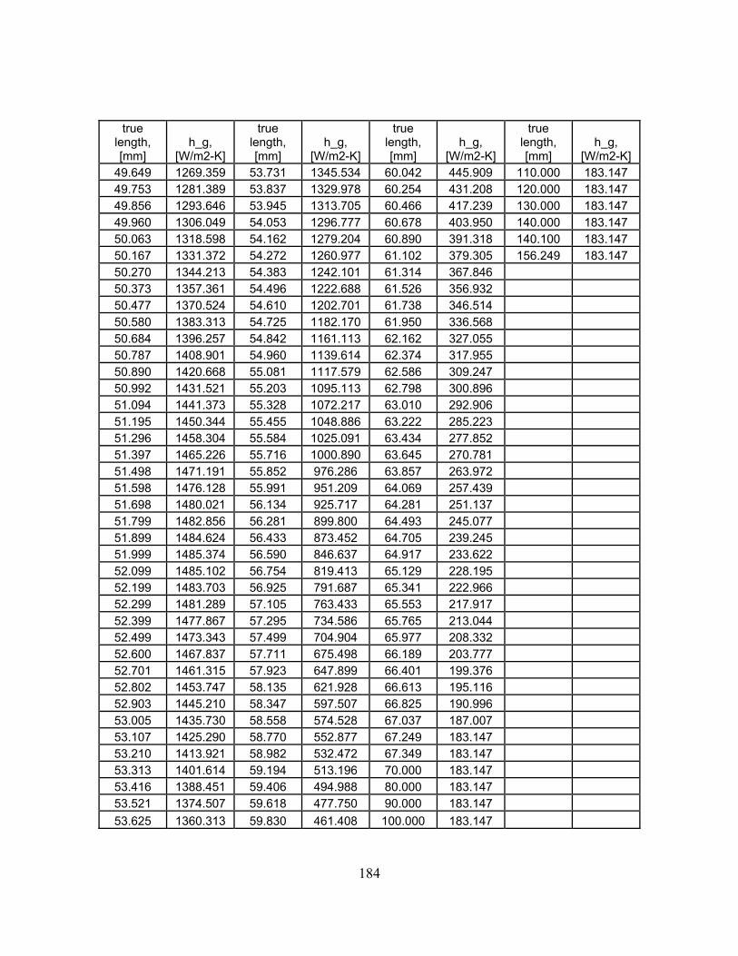
184
true length, [mm]
h_g, [W/m2-K]
true length, [mm]
h_g, [W/m2-K]
true length, [mm]
h_g, [W/m2-K]
true length, [mm]
h_g, [W/m2-K]
49.649 1269.359 53.731 1345.534 60.042 445.909 110.000 183.147 49.753 1281.389 53.837 1329.978 60.254 431.208 120.000 183.147 49.856 1293.646 53.945 1313.705 60.466 417.239 130.000 183.147 49.960 1306.049 54.053 1296.777 60.678 403.950 140.000 183.147 50.063 1318.598 54.162 1279.204 60.890 391.318 140.100 183.147 50.167 1331.372 54.272 1260.977 61.102 379.305 156.249 183.147 50.270 1344.213 54.383 1242.101 61.314 367.846 50.373 1357.361 54.496 1222.688 61.526 356.932 50.477 1370.524 54.610 1202.701 61.738 346.514 50.580 1383.313 54.725 1182.170 61.950 336.568 50.684 1396.257 54.842 1161.113 62.162 327.055 50.787 1408.901 54.960 1139.614 62.374 317.955 50.890 1420.668 55.081 1117.579 62.586 309.247 50.992 1431.521 55.203 1095.113 62.798 300.896 51.094 1441.373 55.328 1072.217 63.010 292.906 51.195 1450.344 55.455 1048.886 63.222 285.223 51.296 1458.304 55.584 1025.091 63.434 277.852 51.397 1465.226 55.716 1000.890 63.645 270.781 51.498 1471.191 55.852 976.286 63.857 263.972 51.598 1476.128 55.991 951.209 64.069 257.439 51.698 1480.021 56.134 925.717 64.281 251.137 51.799 1482.856 56.281 899.800 64.493 245.077 51.899 1484.624 56.433 873.452 64.705 239.245 51.999 1485.374 56.590 846.637 64.917 233.622 52.099 1485.102 56.754 819.413 65.129 228.195 52.199 1483.703 56.925 791.687 65.341 222.966 52.299 1481.289 57.105 763.433 65.553 217.917 52.399 1477.867 57.295 734.586 65.765 213.044 52.499 1473.343 57.499 704.904 65.977 208.332 52.600 1467.837 57.711 675.498 66.189 203.777 52.701 1461.315 57.923 647.899 66.401 199.376 52.802 1453.747 58.135 621.928 66.613 195.116 52.903 1445.210 58.347 597.507 66.825 190.996 53.005 1435.730 58.558 574.528 67.037 187.007 53.107 1425.290 58.770 552.877 67.249 183.147 53.210 1413.921 58.982 532.472 67.349 183.147 53.313 1401.614 59.194 513.196 70.000 183.147 53.416 1388.451 59.406 494.988 80.000 183.147 53.521 1374.507 59.618 477.750 90.000 183.147
53.625 1360.313 59.830 461.408 100.000 183.147

185
APPENDIX III: MATLAB Code to Iterate the Fin Height Equation
% 1/25/11 to 3/15/11 % %%%%%%%%%%%%%%%%%%%%%%%%%%% % % this code iterates the heat transfer theory equation for the height of a % cooling channel with the various equations for the heat % transfer coefficient of convection inside a cooling channel; see other % notes for details % %%%%%%%%%%%%%%%%%%%%%%%%%%% clc clear % constants and knowns: hmax = 0.008; % max channel height by fabrication constraint, [m] % minimum and maximum number of cooling channels to iterate for, calculated % such that the channel widths are guaranteed to fall within the machining % and stress limits because these two numbers are calculated based on % those limits, by hand: ncmin = 19; % minimum number of cooling channels to iterate for, calculated ncmax = 37; % maximum number of cooling channels to iterate for, calculated nciter = ncmax-ncmin+1; %%%debug%%% 2; % total number of iterations for n_c cp_bm = 2222; % specific heat of methane, standard reference temperature % FLUENT Material Database constant, [J/kg-K] lambda_bm = 0.0332; % thermal conductivity of methane, s.r.t.F.M.D.c., [W/m-K] mu_bm = 1.087e-5; % viscosity of methane, s.r.t.F.M.D.c., [kg/m-s] mdot_t = 0.018; % total mass flow rate of methane, ref. [9], [kg/s] r_o = 0.006248; % outer radius of nozzle at throat, calculated, [m] hinitial = 0.001; %%%debug%%% 0.00001 % initial guess for the fin height [m] deltah = 0.0001; % delta h for adding incremental height at each iteration [m] lambda_f = 295; % thermal conductivity of NARloy-Z, ref. [25], [W/m-K] T_co = 298.15; % standard reference temperature for "coolant bulk % temperature", [K] T_wc = 533; % coolant side wall temperature, ref. [16], [K] mu_w = 1.7525e-5; % coolant (methane) viscosity at coolant-side wall % temperature T_wc, calculated, [kg/m-s] diff = zeros(1,2); % initiate dummy difference variable converge = 1.0e-6; % convergence criteria hi = zeros(1,2); % iteration values holder for h % matrix of solutions: % rows = range of n_c values % column 1 = n_c value % column 2 = w value for n_c [m] % column 3 = delta_f value for n_c [m] % column 4 = mdot_c for n_c [kg/s] % column 5 = alpha_g_1 value [W/m2-K]
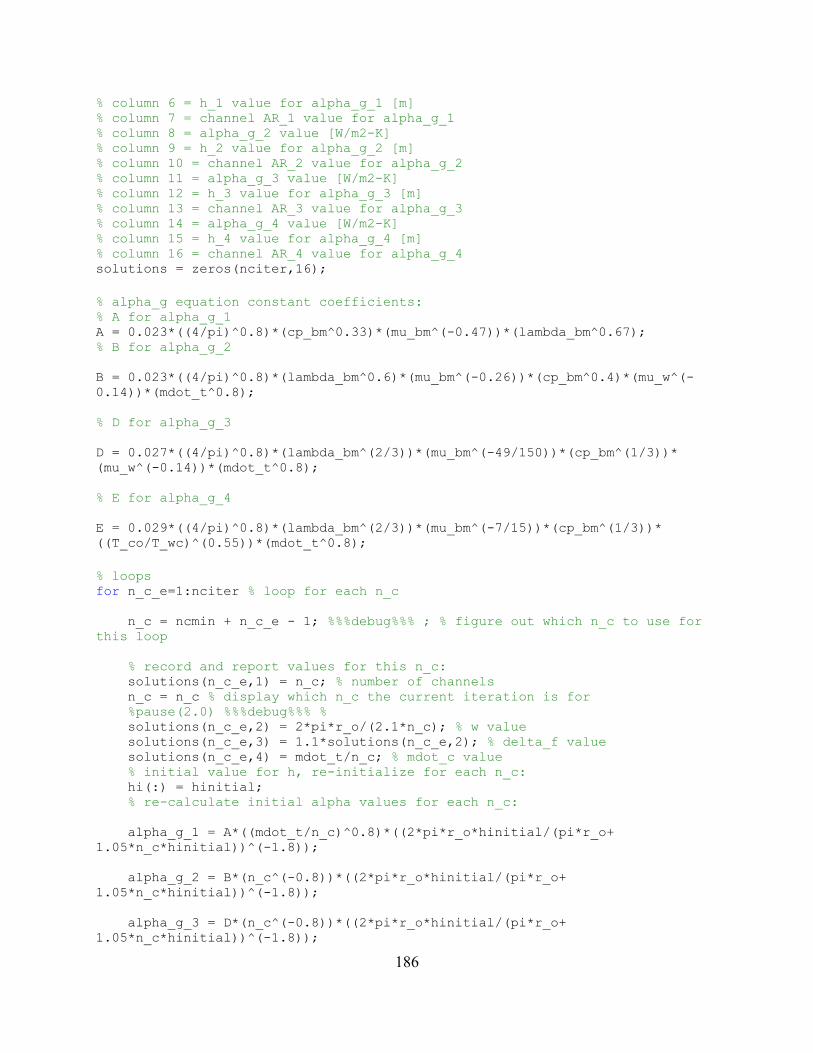
186
% column 6 = h_1 value for alpha_g_1 [m] % column 7 = channel AR_1 value for alpha_g_1 % column 8 = alpha_g_2 value [W/m2-K] % column 9 = h_2 value for alpha_g_2 [m] % column 10 = channel AR_2 value for alpha_g_2 % column 11 = alpha_g_3 value [W/m2-K] % column 12 = h_3 value for alpha_g_3 [m] % column 13 = channel AR_3 value for alpha_g_3 % column 14 = alpha_g_4 value [W/m2-K] % column 15 = h_4 value for alpha_g_4 [m] % column 16 = channel AR_4 value for alpha_g_4 solutions = zeros(nciter,16); % alpha_g equation constant coefficients: % A for alpha_g_1 A = 0.023*((4/pi)^0.8)*(cp_bm^0.33)*(mu_bm^(-0.47))*(lambda_bm^0.67); % B for alpha_g_2 B = 0.023*((4/pi)^0.8)*(lambda_bm^0.6)*(mu_bm^(-0.26))*(cp_bm^0.4)*(mu_w^(-0.14))*(mdot_t^0.8); % D for alpha_g_3 D = 0.027*((4/pi)^0.8)*(lambda_bm^(2/3))*(mu_bm^(-49/150))*(cp_bm^(1/3))* (mu_w^(-0.14))*(mdot_t^0.8); % E for alpha_g_4 E = 0.029*((4/pi)^0.8)*(lambda_bm^(2/3))*(mu_bm^(-7/15))*(cp_bm^(1/3))* ((T_co/T_wc)^(0.55))*(mdot_t^0.8); % loops for n_c_e=1:nciter % loop for each n_c n_c = ncmin + n_c_e - 1; %%%debug%%% ; % figure out which n_c to use for this loop % record and report values for this n_c: solutions(n_c_e,1) = n_c; % number of channels n_c = n_c % display which n_c the current iteration is for %pause(2.0) %%%debug%%% % solutions(n_c_e,2) = 2*pi*r_o/(2.1*n_c); % w value solutions(n_c_e,3) = 1.1*solutions(n_c_e,2); % delta_f value solutions(n_c_e,4) = mdot_t/n_c; % mdot_c value % initial value for h, re-initialize for each n_c: hi(:) = hinitial; % re-calculate initial alpha values for each n_c: alpha_g_1 = A*((mdot_t/n_c)^0.8)*((2*pi*r_o*hinitial/(pi*r_o+ 1.05*n_c*hinitial))^(-1.8)); alpha_g_2 = B*(n_c^(-0.8))*((2*pi*r_o*hinitial/(pi*r_o+ 1.05*n_c*hinitial))^(-1.8)); alpha_g_3 = D*(n_c^(-0.8))*((2*pi*r_o*hinitial/(pi*r_o+ 1.05*n_c*hinitial))^(-1.8));

187
alpha_g_4 = E*(n_c^(-0.8))*((2*pi*r_o*hinitial/(pi*r_o+ 1.05*n_c*hinitial))^(-1.8)); diff(:) = 1000; % re-initialize for each n_c for n_alpha=1:4 %loop for each alpha_g %n_alpha = n_alpha %%%debug%%% % % choose which initial alpha_g value to use and set index to store solution if (n_alpha == 1) alpha_g = alpha_g_1; index = 5; elseif (n_alpha == 2) alpha_g = alpha_g_2; index = 8; elseif (n_alpha == 3) alpha_g = alpha_g_3; index = 11; else alpha_g = alpha_g_4; index = 14; end hi(:) = hinitial; % re-initialize for each alpha_g (which use hinitial) diff(:) = 1000; % re-initialize for each alpha_g ee = 0; % WHILE loop counter, re-initialize for each alpha_g % loop to iterate h while (diff(1,1) > converge) ee = ee + 1; hi(1,2) = 1.4192*((11*pi*r_o*lambda_f/(21*n_c))^0.5)* (alpha_g^(-0.5))-(11*pi*r_o/(21*n_c)); %%%debug%%% ; diff(1,2) = abs(hi(1,2)-hi(1,1)); %%%debug%%% ; %pause(2.0) %%%debug%%% % % multiplier to handle divergence if (diff(1,2) >= diff(1,1)) diff(:) = 1000; % reset value to initial if diverging to start over deltahmult = -1; % make hinitial smaller else deltahmult = 0; end % multiplier to handle negative values of h if (hi(1,2) <= 0.0) hi(1,2) = hinitial + deltah*ee; % reset value to initial plus more each time deltahmult = 5; % add a lot more of deltah

188
diff(:) = 1000; % reset since reseting hi else deltahmult = 0; end % store the alpha_g value before calculating a new one for the % next loop since the current value will correspond to the % converged h: solutions(n_c_e,index) = alpha_g; % prepare for next loop: % set current/new hi(1,2) to previous hi(1,1): hi(1,1) = hi(1,2) + deltahmult*deltah; %hi(1,1) = hi(1,1) %%%debug%%% % %pause(2.0) %%%debug%%% % % set current diff to previous diff to loop: diff(1,1) = diff(1,2); % calculate a new alpha_g for the next WHILE loop, depending % on which alpha_g is being used for the current WHILE loop: if (n_alpha == 1) alpha_g_1 = A*((mdot_t/n_c)^0.8)*((2*pi*r_o*hi(1,1)/(pi*r_o+ 1.05*n_c*hi(1,1)))^(-1.8)); alpha_g = alpha_g_1; elseif (n_alpha == 2) alpha_g_2 = B*(n_c^(-0.8))*((2*pi*r_o*hi(1,1)/(pi*r_o+ 1.05*n_c*hi(1,1)))^(-1.8)); alpha_g = alpha_g_2; elseif (n_alpha == 3) alpha_g_3 = D*(n_c^(-0.8))*((2*pi*r_o*hi(1,1)/(pi*r_o+ 1.05*n_c*hi(1,1)))^(-1.8)); alpha_g = alpha_g_3; else alpha_g_4 = E*(n_c^(-0.8))*((2*pi*r_o*hi(1,1)/(pi*r_o+ 1.05*n_c*hi(1,1)))^(-1.8)); alpha_g = alpha_g_4; end end % diff(1,1) = diff(1,1) %%%debug%%% % %converge = converge %%%debug%%% % %pause(2.0) %%%debug%%% % % handle machining restriction and save the associated alpha: if (hi(1,1) > hmax) hi(1,1) = hmax if (n_alpha == 1) alpha_g_1 = A*((mdot_t/n_c)^0.8)*((2*pi*r_o*hi(1,1)/(pi*r_o+ 1.05*n_c*hi(1,1)))^(-1.8)); alpha_g = alpha_g_1; elseif (n_alpha == 2)

189
alpha_g_2 = B*(n_c^(-0.8))*((2*pi*r_o*hi(1,1)/(pi*r_o+ 1.05*n_c*hi(1,1)))^(-1.8)); alpha_g = alpha_g_2; elseif (n_alpha == 3) alpha_g_3 = D*(n_c^(-0.8))*((2*pi*r_o*hi(1,1)/(pi*r_o+ 1.05*n_c*hi(1,1)))^(-1.8)); alpha_g = alpha_g_3; else alpha_g_4 = E*(n_c^(-0.8))*((2*pi*r_o*hi(1,1)/(pi*r_o+ 1.05*n_c*hi(1,1)))^(-1.8)); alpha_g = alpha_g_4; end solutions(n_c_e,index) = alpha_g; end % record and report values for this n_c and alpha_g: solutions(n_c_e,index+1) = hi(1,1); % h value, (1,1) because a % new (1,2) will not be % recalculated anyway hi(1,1) = hi(1,1) % display the determined h value %pause(2.0) %%%debug%%% % solutions(n_c_e,index+2) = hi(1,1)/solutions(n_c_e,2); % channel AR value end end % % end of program

190
APPENDIX IV: Results of Fin Height Iteration
The results of the fin height iteration are presented in one table in three parts, broken at the
jagged lines.
number of
channels, n_c
channel width, w, [m]
fin width, delta_f, [m]
mass flow rate per channel, mdot_c,
[kg/s]
heat transfer
coefficient 1,
alpha_g_1, [W/m2-k]
channel (and fin) height,
h_1, [m]
channel AR,
AR_1
19 0.0009839 0.0010823 0.00094737 2722.4 0.008 8.13120 0.0009347 0.0010282 0.0009 2837.5 0.008 8.5589
21 0.0008902 0.00097921 0.00085714 2952.7 0.008 8.9869
22 0.0008497 0.0009347 0.00081818 3068 0.008 9.414823 0.0008128 0.00089406 0.00078261 3183.4 0.008 9.842724 0.0007789 0.00085681 0.00075 3298.8 0.008 10.27125 0.0007478 0.00082253 0.00072 3414.4 0.008 10.69926 0.0007190 0.0007909 0.00069231 3547.4 0.0077431 10.76927 0.0006924 0.00076161 0.00066667 3683.8 0.0074563 10.76928 0.0006676 0.00073441 0.00064286 3820.2 0.00719 10.76929 0.0006446 0.00070908 0.00062069 3956.7 0.0069421 10.76930 0.0006231 0.00068545 0.0006 4093.1 0.0067107 10.76931 0.0006030 0.00066333 0.00058065 4229.5 0.0064942 10.76932 0.0005842 0.00064261 0.0005625 4366 0.0062913 10.76933 0.0005665 0.00062313 0.00054545 4502.4 0.0061006 10.76934 0.0005498 0.0006048 0.00052941 4638.9 0.0059212 10.76935 0.0005341 0.00058752 0.00051429 4775.3 0.005752 10.76936 0.0005193 0.0005712 0.0005 4911.9 0.0055922 10.769
37 0.0005052 0.00055577 0.00048649 5048.3 0.005441 10.769

191
heat transfer
coefficient 2,
alpha_g_2, [W/m2-k]
channel (and fin) height,
h_2, [m]
channel AR,
AR_2
heat transfer
coefficient 3,
alpha_g_3, [W/m2-k]
channel (and fin) height,
h_3, [m]
channel AR,
AR_3
heat transfer
coefficient 4,
alpha_g_4, [W/m2-k]
channel (and fin) height,
h_4, [m]
2490.2 0.008 8.131 2985.9 0.008 8.131 2491.1 0.0082595.5 0.008 8.5589 3112.2 0.008 8.5589 2596.4 0.008
2700.9 0.008 8.9869 3238.5 0.008 8.9869 2701.9 0.0082806.3 0.008 9.4148 3365 0.008 9.4148 2807.4 0.0082911.9 0.008 9.8427 3491.6 0.008 9.8427 2913 0.0083017.5 0.008 10.271 3621.5 0.0079553 10.213 3018.6 0.0083123.2 0.008 10.699 3772.4 0.0076371 10.213 3124.3 0.0083228.9 0.008 11.127 3923.3 0.0073434 10.213 3230.1 0.0083344.2 0.0078447 11.33 4074.2 0.0070714 10.213 3345.5 0.007843
3468 0.0075645 11.33 4225.1 0.0068189 10.213 3469.4 0.00756293591.9 0.0073036 11.33 4376 0.0065837 10.213 3593.3 0.00730213715.8 0.0070602 11.33 4526.9 0.0063643 10.213 3717.2 0.00705873839.6 0.0068324 11.33 4677.7 0.006159 10.213 3841.1 0.0068313963.5 0.0066189 11.33 4828.6 0.0059665 10.213 3965.1 0.00661754087.3 0.0064184 11.33 4979.5 0.0057857 10.213 4089 0.0064174211.2 0.0062296 11.33 5130.4 0.0056155 10.213 4212.9 0.00622834335.1 0.0060515 11.33 5281.3 0.0054551 10.213 4336.9 0.0060503
4459 0.0058834 11.33 5432.2 0.0053036 10.213 4460.8 0.0058822
4582.9 0.0057244 11.33 5583.1 0.0051602 10.213 4584.7 0.0057232

192
channel AR,
AR_4 average
alpha average height
channel half width,
[m] fin half
width, [m]
channel half width +
fin half width, [m]
8.131 2672.4 0.008 0.00049195 0.00054115 0.00103310 8.5589 2785.4 0.008 0.00046735 0.00051410 0.00098145
8.9869 2898.5 0.008 0.00044510 0.00048961 0.00093470
9.4148 3011.675 0.0080000 0.00042487 0.00046735 0.00089222 use 9.8427 3124.975 0.0080000 0.00040639 0.00044703 0.00085342 these 10.271 3239.1 0.0079888 0.00038946 0.00042841 0.00081787 channels10.699 3358.575 0.0079093 0.00037388 0.00041127 0.00078515 only 11.127 3482.425 0.0077716 0.00035950 0.00039545 0.00075495 11.328 3611.925 0.0075539 0.00034619 0.00038081 0.00072699 11.328 3745.675 0.0072841 0.00033382 0.00036721 0.00070103 11.328 3879.475 0.0070329 0.00032231 0.00035454 0.00067685 11.328 4013.25 0.0067985 0.00031157 0.00034273 0.00065429 11.328 4146.975 0.0065792 0.00030152 0.00033167 0.00063318 11.328 4280.8 0.0063736 0.00029210 0.00032131 0.00061340 11.328 4414.55 0.0061804 0.00028324 0.00031157 0.00059481 11.328 4548.35 0.0059987 0.00027491 0.00030240 0.00057731 11.328 4682.15 0.0058272 0.00026706 0.00029376 0.00056082 11.328 4815.975 0.0056654 0.00025964 0.00028560 0.00054524
11.328 4949.75 0.0055122 0.00025262 0.00027789 0.00053051

193
APPENDIX V: Drawing Coordinates for CFD geometry
n_c = 22 n_c = 23 ( x y z ) mm ( x y z ) mm
A = 0 0 0 A = 0 0 0 B = -156.249 0 1.0980 B = -156.249 0 1.0980 C = -156.249 0 9.0980 C = -156.249 0 9.0980 D = -156.249 0.4249 9.0980 D = -156.249 0.4064 9.0980 E = -156.249 0.4249 1.0980 E = -156.249 0.4064 1.0980 F = 0 0 1.0980 F = 0 0 1.0980 G = 0 0.4249 1.0980 G = 0 0.4064 1.0980 H = 0 0.4249 9.0980 H = 0 0.4064 9.0980 I = 0 0.8922 9.0980 I = 0 0.8534 9.0980 J = 0 0.8922 0 J = 0 0.8534 0 K = 0 0 9.0980 K = 0 0 9.0980 L = 0 0 10.0980 L = 0 0 10.0980 M = 0 0.8922 10.0980 M = 0 0.8534 10.0980
n_c = 24 n_c = 25
( x y z ) mm ( x y z ) mm A = 0 0 0 A = 0 0 0 B = -156.249 0 1.0980 B = -156.249 0 1.0980 C = -156.249 0 9.0868 C = -156.249 0 9.0073 D = -156.249 0.3895 9.0868 D = -156.249 0.3739 9.0073 E = -156.249 0.3895 1.0980 E = -156.249 0.3739 1.0980 F = 0 0 1.0980 F = 0 0 1.0980 G = 0 0.3895 1.0980 G = 0 0.3739 1.0980 H = 0 0.3895 9.0868 H = 0 0.3739 9.0073 I = 0 0.8179 9.0868 I = 0 0.7851 9.0073 J = 0 0.8179 0 J = 0 0.7851 0 K = 0 0 9.0868 K = 0 0 9.0073 L = 0 0 10.0868 L = 0 0 10.0073 M = 0 0.8179 10.0868 M = 0 0.7851 10.0073

194
n_c = 26 n_c = 27 ( x y z ) mm ( x y z ) mm
A = 0 0 0 A = 0 0 0 B = -156.249 0 1.0980 B = -156.249 0 1.0980 C = -156.249 0 8.8696 C = -156.249 0 8.6519 D = -156.249 0.3595 8.8696 D = -156.249 0.3462 8.6519 E = -156.249 0.3595 1.0980 E = -156.249 0.3462 1.0980 F = 0 0 1.0980 F = 0 0 1.0980 G = 0 0.3595 1.0980 G = 0 0.3462 1.0980 H = 0 0.3595 8.8696 H = 0 0.3462 8.6519 I = 0 0.7550 8.8696 I = 0 0.7270 8.6519 J = 0 0.7550 0 J = 0 0.7270 0 K = 0 0 8.8696 K = 0 0 8.6519 L = 0 0 9.8696 L = 0 0 9.6519 M = 0 0.7550 9.8696 M = 0 0.7270 9.6519
n_c = 28 n_c = 29
( x y z ) mm ( x y z ) mm A = 0 0 0 A = 0 0 0 B = -156.249 0 1.0980 B = -156.249 0 1.0980 C = -156.249 0 8.3821 C = -156.249 0 8.1309 D = -156.249 0.3338 8.3821 D = -156.249 0.3223 8.1309 E = -156.249 0.3338 1.0980 E = -156.249 0.3223 1.0980 F = 0 0 1.0980 F = 0 0 1.0980 G = 0 0.3338 1.0980 G = 0 0.3223 1.0980 H = 0 0.3338 8.3821 H = 0 0.3223 8.1309 I = 0 0.7010 8.3821 I = 0 0.6769 8.1309 J = 0 0.7010 0 J = 0 0.6769 0 K = 0 0 8.3821 K = 0 0 8.1309 L = 0 0 9.3821 L = 0 0 9.1309 M = 0 0.7010 9.3821 M = 0 0.6769 9.1309

195
n_c = 30 n_c = 31 ( x y z ) mm ( x y z ) mm
A = 0 0 0 A = 0 0 0 B = -156.249 0 1.0980 B = -156.249 0 1.0980 C = -156.249 0 7.8965 C = -156.249 0 7.6772 D = -156.249 0.3116 7.8965 D = -156.249 0.3015 7.6772 E = -156.249 0.3116 1.0980 E = -156.249 0.3015 1.0980 F = 0 0 1.0980 F = 0 0 1.0980 G = 0 0.3116 1.0980 G = 0 0.3015 1.0980 H = 0 0.3116 7.8965 H = 0 0.3015 7.6772 I = 0 0.6543 7.8965 I = 0 0.6332 7.6772 J = 0 0.6543 0 J = 0 0.6332 0 K = 0 0 7.8965 K = 0 0 7.6772 L = 0 0 8.8965 L = 0 0 8.6772 M = 0 0.6543 8.8965 M = 0 0.6332 8.6772
n_c = 32 n_c = 33
( x y z ) mm ( x y z ) mm A = 0 0 0 A = 0 0 0 B = -156.249 0 1.0980 B = -156.249 0 1.0980 C = -156.249 0 7.4716 C = -156.249 0 7.2784 D = -156.249 0.2921 7.4716 D = -156.249 0.2832 7.2784 E = -156.249 0.2921 1.0980 E = -156.249 0.2832 1.0980 F = 0 0 1.0980 F = 0 0 1.0980 G = 0 0.2921 1.0980 G = 0 0.2832 1.0980 H = 0 0.2921 7.4716 H = 0 0.2832 7.2784 I = 0 0.6134 7.4716 I = 0 0.5948 7.2784 J = 0 0.6134 0 J = 0 0.5948 0 K = 0 0 7.4716 K = 0 0 7.2784 L = 0 0 8.4716 L = 0 0 8.2784 M = 0 0.6134 8.4716 M = 0 0.5948 8.2784

196
n_c = 34 n_c = 35 ( x y z ) mm ( x y z ) mm
A = 0 0 0 A = 0 0 0 B = -156.249 0 1.0980 B = -156.249 0 1.0980 C = -156.249 0 7.0967 C = -156.249 0 6.9252 D = -156.249 0.2749 7.0967 D = -156.249 0.2671 6.9252 E = -156.249 0.2749 1.0980 E = -156.249 0.2671 1.0980 F = 0 0 1.0980 F = 0 0 1.0980 G = 0 0.2749 1.0980 G = 0 0.2671 1.0980 H = 0 0.2749 7.0967 H = 0 0.2671 6.9252 I = 0 0.5773 7.0967 I = 0 0.5608 6.9252 J = 0 0.5773 0 J = 0 0.5608 0 K = 0 0 7.0967 K = 0 0 6.9252 L = 0 0 8.0967 L = 0 0 7.9252 M = 0 0.5773 8.0967 M = 0 0.5608 7.9252
n_c = 36 n_c = 37
( x y z ) mm ( x y z ) mm A = 0 0 0 A = 0 0 0 B = -156.249 0 1.0980 B = -156.249 0 1.0980 C = -156.249 0 6.7634 C = -156.249 0 6.6102 D = -156.249 0.2596 6.7634 D = -156.249 0.2526 6.6102 E = -156.249 0.2596 1.0980 E = -156.249 0.2526 1.0980 F = 0 0 1.0980 F = 0 0 1.0980 G = 0 0.2596 1.0980 G = 0 0.2526 1.0980 H = 0 0.2596 6.7634 H = 0 0.2526 6.6102 I = 0 0.5452 6.7634 I = 0 0.5305 6.6102 J = 0 0.5452 0 J = 0 0.5305 0 K = 0 0 6.7634 K = 0 0 6.6102 L = 0 0 7.7634 L = 0 0 7.6102 M = 0 0.5452 7.7634 M = 0 0.5305 7.6102

197
CURRICULUM VITA
Christopher Bradford is a native (odd to most locals) of El Paso, Texas, graduating from Andress
High School in the top 3% of the May 1999 class. Moving on with ephemeral hope for the
future, he soon discovered the inadequate preparedness for college and an indication into the true
nature of human interaction that his prior years had not afforded. Transferring from The
University of Arizona and New Mexico State University, he eventually graduated with a
Bachelor of Science degree in Aerospace Engineering from Texas A&M University in May of
2005, although at many times he imagined the benefit of attending a different university. Soon
after graduation he realized the negative potential that a lack of knowledge in other fields of
study could have on his future, discovering through experience that simply following a
standardized curriculum does not necessarily guarantee a person has much intelligence. He thus
began taking the initiative to learn from many fields including philosophy, sociology, physics,
and other engineering disciplines to supplement his multiple interests and talents, as he
highlights at www.myspace.com/christopher_aerospace, if hosting services remain available.
While daydreaming, he often ponders the futility of personal human desires, and the true value of
money. However, he provides non-legally-binding,, no-liability, academic-style consultation
services for a nominal fee when scheduled in advance at "christopherbradford at yahoo dot com"
(if email services remain available), because he realized from Plato's writings on Socrates that
knowledge itself may fulfill the intellect but not necessarily the stomach. Returning to academia
after multiple career ventures, he expects to earn a Master of Science degree in Mechanical
Engineering from The University of Texas at El Paso in the summer of 2011. Christopher does
not consider himself to reside at any permanent address, for various reasons.


![REGENERATIVE BRAKING SYSTEM IN ELECTRIC VEHICLES · REGENERATIVE BRAKING SYSTEM IN ELECTRIC VEHICLES ... REGENERATIVE BRAKING SYSTEM ... Regenerative action during braking[9].](https://static.cupdf.com/doc/110x72/5adccef67f8b9a1a088c7cf0/regenerative-braking-system-in-electric-vehicles-braking-system-in-electric-vehicles.jpg)
