i
OKON, UBOKUDOM ETIM
PG/Ph.D/10/ 58105
ASSESSMENT OF INCOME GENERATING ACTIVITIES AMONG URBAN FARM HOUSEHOLDS IN SOUTH-SOUTH NIGERIA
FACULTY OF AGRICULTURE
DEPARTMENT OF AGRICULTURAL ECONOMICS
Ebere Omeje Digitally Signed by: Content manager’s Name
DN : CN = Webmaster’s name
O= University of Nigeria, Nsukka
OU = Innovation Centre
ii
ASSESSMENT OF INCOME GENERATING ACTIVITIES AMONG UR BAN FARM HOUSEHOLDS IN SOUTH-SOUTH NIGERIA
BY
OKON, UBOKUDOM ETIM
PG/Ph.D/10/ 58105
DEPARTMENT OF AGRICULTURAL ECONOMICS
UNIVERSITY OF NIGERIA, NSUKKA
DECEMBER, 2014
i
ASSESSMENT OF INCOME GENERATING ACTIVITIES AMONG UR BAN FARM HOUSEHOLDS IN SOUTH-SOUTH NIGERIA
A Ph.D THESIS SUBMITTED TO THE DEPARTMENT OF AGRICU LTURAL ECONOMICS, UNIVERSITY OF NIGERIA, NSUKKA, IN PARTIA L FULFILMENT OF THE REQUIREMENTS FOR THE AWARD OF THE DEGREE OF DOCTOR OF
PHILOSOPHY IN AGRICULTURAL ECONOMICS
BY
OKON, UBOKUDOM ETIM
PG/Ph.D/10/ 58105
DEPARTMENT OF AGRICULTURAL ECONOMICS, UNIVERSITY OF NIGERIA, NSUKKA
DECEMBER, 2014
ii
---------------------------- -------------- ------------------------------ -------------- PROF. E. C. OKORJI Date DR. A. A. ENETE Date (Supervisor) (Supervisor) ------------------------------------ -------------- ---------------------------- ------------ PROF. S. A. N. D. CHIDEBELU Date External Examiner Date (Head of Department)
CERTIFICATION
Mr OKON, UBOKUDOM ETIM, a postgraduate student of the Department of Agricultural
Economics, University of Nigeria, Nsukka with Registration Number PG/Ph.D/10/58105 has
satisfactorily completed the requirements for research work for the award of the degree of Doctor
of Philosophy (Ph.D) in Agricultural Economics. The work embodied in this thesis is original
and has not been submitted in part or full for any other diploma or degree in this or any other
University.

iii
DEDICATION
To God, to whom I return all the Glory and Honour; and to my Son Aniekeme-Abasi Okon
iv
ACKNOWLEDGEMENTS
In the name of God Almighty the most merciful, compassionate and beneficent who bestowed
me with intellect, strength, enthusiasm and patience to this challenging task of Ph.D. Without his
blessings, I would not be able to complete this demanding job. I am grateful from the core of my
heart to Prof. E. C. Okorji, my major supervisor whose direction; efforts and encouragement
aided the outcome of this study. He was there for me just like a father would for his son. I deeply
appreciate the new insights that our interaction brought into the work. He provided me his
excellent guidance and enthusiastic support for my research and professional development. His
guidance, suggestions, and constructive criticisms during the whole period of my research
project contributed a lot to improve the final outcome from this research investigation.
I express my profound gratitude to Dr. A.A. Enete, my second supervisor; his constructive
criticism during my master’s work provided me an opportunity to improve my research skills.
His thoughtful advice often serves to give me a sense of direction during my studies. I will not
forget late Prof. E.C. Nwagbo, who gave me the fundamentals of farm management during our
farm management classes. I appreciate the contributions of the Head of Department Prof.
S.A.N.D. Chidebelu and other lecturers in the Department, Prof. Arua, Prof. N.J. Nweze, Prof.
E.C. Eboh, Prof. C. J. Arene, Prof. C.U. Okoye, Prof. Achike, Dr. F. U. Agbo, Dr. Okpupara, Dr.
Chukwuone, Dr. Amechina, Mr Onyekuru, Mrs R. Arua, and Mrs Onyenekwe. The
administrative staff, Mrs Romaine, Blessing and all PG students for their contributions during
the first draft of this work at the departmental seminar.
My special appreciation to Bishop Etuk Eka, for his prayers, counseling, advice, and
encouragement to my family during this challenging period. A bundle of thanks are to my friends
Dr. Idorenyin Udoh, Mr Jude Nwankwo, Mr Aniefiok Udoh, Mr Ukeme Ene, Dr. Taofeeq
v
Amusa, Dr. Nsikan Bassey, Dr. Taru Bala, Dr Ndifreke Umohudo, Dr I. E. Ele, Mr. Nseobong
Okpura, Mr Nseobong Uto, Mr Ifreke Udoidem, Mr Anthony Ekpo, Eng. Aniekan Ikpe, Mr
Sebastian Etefia, Pastor Abel, and Offiong Ukpe. I also acknowledge the support of Dr I. C.
Idiong, for his worthy time and mentoring during my research career. I offer my deepest sense of
gratitude to my late parent whose care, support and advice guided me through the storms of this
world. My special thank goes to my most elder sister Mrs Enebong Solomon for her prayers,
moral and financial support without which the Ph.D work would not have been fruitful. She gave
me a hand during the hard times, when I felt hopeless; I will never forget what she did for me.
My thanks and affection will always be available to her. My appreciation also goes to all my
siblings Mr Aniekan-abasi Okon, Mrs Ememobong Atakpa, Ms Enobong Okon, Mr & Mrs John
Akpan, my nephews and nieces Ubong, Kufre, Solomon, Edidiong, Deborah, Emmanuel etc and
my Inlaws Mr and Mrs M.O. Olutunbi and family.
Finally, am indebted to my wife, Deborah Ubokudom Okon and my Son, Aniekeme-Abasi Okon
for their continued support, Prayers, sacrifices and hardship they faced during this Ph.D work. I
truly appreciate their love, understanding, sufferings and patience. I also thank all whose names
are not mentioned here but played significant roles in this research work.
vi
ABSTRACT
The study analyzed the income generating activities among urban farm households in South-
south Nigeria. Primary data were collected using structured questionnaires administered to two
hundred and eighty nine urban farm households, which were selected by purposive, and simple
random sampling techniques. The data were analyzed using descriptive statistics, Ordinary least
squares, multinomial logit, quantile regression and vulnerability index analysis. The results
showed that majority (66%) of the respondents were male, with mean age of 44 years. All
respondents were literate with at least secondary education. Average farming experience was 9
years. About 47.05% of the respondents practiced sole cropping with vegetables as their major
crop. Non-agricultural wage income (36%) and crop production income (26%) were major
income generating activities practiced by the respondents. All respondents owned mobile
phones. Only 37% of the respondents owned land. About 39%, 22%, 21%, and 32% of the
respondents owned refrigerators, tricycles, cars, and other equipment respectively. The
explanatory variables such as land size and asset value positively and significantly (p < 0.01)
influenced livestock production income. In addition to land size and asset value, farming
experience had positive and significant (p < 0.01) influence, while household size had negative
and significant (p < 0.05) influence on crop production income. Compared to non-agricultural
wage income, farm size (p < 0.01), gender (p < 0.01), years of formal education (p < 0.01), and
farming experience (p < 0.05) were the major determinants of households’ participation in
agricultural wage income category, while years of formal education (p < 0.01) and age of
household heads (p < 0.05) were the major determinants of households’ participation in non-
agricultural wage income category. Quantile regression results showed that age, gender, land
size, asset value, and non-farm income positively and significantly (p < 0.01) influenced farm
income at 75th quantile, while farm location, years of formal education, farming experience,
marital status, household size, loan access, market proximity negatively and significantly (p <
0.01) influenced farm income also at 75th quantile. Vulnerability index analysis showed that
urban farm households were 55% more likely to be vulnerable to economic shocks. The results
call for policies aimed at making land more available to urban farmers by incorporating urban
farming in developmental planning processes, redesigning of urban centers, boosting
households’ asset and encouraging households to participate in urban farming for poverty
reduction and food security.
vii TABLE OF CONTENTS
Page
Title Page i
Certification ii
Dedication iii
Acknowledgements iv
Abstract vi
Table of Content vii
List of Tables viii
List of Figures ix
CHAPTER ONE: INTRODUCTION
1.1 Background of the Study 1
1.2 Problem Statement 6
1.3 Objectives of the Study 10
1.4 Hypotheses of the Study 11
1.5 Justification of the Study 11
1.6 Limitation of the Study 13
CHAPTER TWO: LITERATURE REVIEW
2.1 Concepts of Household 14
2.2 Sustainable Livelihood Approaches 15
2.3 Urban households Income Generating Activities 19
2.4 Asset and Classification 23
2.4.1 Why assets are important 24
2.4.2 Classification of Asset 25
viii
2.5 Households Asset Utilization 27
2.6 Linking Asset, Activity Choice and Income: Conceptual Approach 27
2.7 Urbanization and Poverty 32
2.8 Urban Agriculture at Household level 34
2.9 Households Vulnerability to Shocks 35
2.9.1 Prevention Strategies 38
2.9.2 Mitigation Strategies 38
2.9.3 Coping Strategies 39
2.9.4 Quantifying Vulnerability 39
2.9.5 Vulnerability as Uninsured Exposure to Risk (VER) 39
2.9.6 Vulnerability as low Expected Utility (VEU) 40
2.9.7 Vulnerability as Expected Poverty (VEP) 40
2.10 Theoretical Framework 41
2.10.1 Utility Theory 41
2.10.2 Sustainability Theory 43
2.10.3 Theories considering Risk Averse Farmers 44
2.11 Analytical Framework 46
2.11.1 Ordinary Least Square (OLS) 46
2.11.2 Multinomial Logit Model (MNL) 47
2.11.3 Quantile Regression 50
ix
CHAPTER THREE: METHODOLOGY
3.1 Study Area 54
3.2 Sampling Procedures 54
3.3 Method of Data Collection 55
3.4 Data Analysis 56
3.4.1 Ordinary Least Squares 57
3.4.2 Multinomial Logit Model (MNL) 58
3.4.3 Quantile Regression Analysis 62
3.4.4 Vulnerability Index Analysis 65
CHAPTER FOUR: RESULTS AND DISCUSSION
4.1.1 Age of the Household Heads 68
4.1.2 Level of Education of the Household Heads 69
4.1.3 Household size of the Respondents 70
4.1.4 Farming Experience of the Household heads 72
4.1.5 Gender of the household heads 72
4.1.6 Marital status of the household heads 72
4.1.7 Distribution of the household heads by income generating activities 73
4.1.8 Level of livelihood asset available to the respondents 75
4.1.9 Production patterns of the Respondents 77
4.2 Respondents Households’ composition 79
x
4.3 Factors that determine households’ level of income from each category of income
generating activity 81
4.4 Socio-economic factors influencing participation in income generating activities by urban
farming households in the study area 86
4.5 Quantile regression estimates of the determinants of farm income among urban farm
households in the study area 93
4.6 Urban farm households’ vulnerability to economic shocks in the study area 99
CHAPTER FIVE: SUMMARY CONCLUSION AND RECOMMENDATION S
5.1 Summary 106
5.2 Conclusion 110
5.3 Recommendations 111
5.4 Contribution to Knowledge 112
5.5 Suggestions for further Research 112
References 113
Appendix 132
xi
LIST OF TABLES
Tables Page
2.1 Some strategies adopted by poor households 17
4.1 Socio-economic characteristics of the respondents 56
4.2 Distribution of household heads by major categories of Income Generating Activities 59
4.3 Frequency distribution of the respondents according to production patterns 60
4.4 Frequency distribution of respondents according to types of livestock and crops grown 61
4.5 Frequency distribution of the respondents according to household Composition 62
4.6 Summary statistics of the respondents total household income 62
4.7 Percentage distribution of respondents by asset ownership 63
4.8 Results of the OLS estimates of factors influencing households’ level of Income from each
category of Income Generating activity 66
4.9 Parameter estimates of the Multinomial logit (MNL) analysis of the Socio-economic factors
influencing Choice of Income Generating activities by the respondents 72
4.10 Marginal effects of the Multinomial logit (MNL) estimates of the Socio-economic factors
influencing Choice of Income Generating activities by the respondents 73
4.11 Quantile regression and OLS estimates of the Determinants of farm income among the respondents 78
4.12 Vulnerability level of the respondents 83
xii
LIST OF FIGURES
Figure Page
2.1 Sustainable livelihood framework 22
2.2 Asset pentagon 21
2.3 Factors influencing households 25
4.1 Bar chart showing percentage distribution of respondents by major categories of Income Generating Activities 59
4.2 Bar chart showing percentage distribution of respondents by asset ownership status 64
4.3 Bar chart showing Vulnerability level of the respondents 84
1
CHAPTER ONE
INTRODUCTION
1.1 Background of the Study
Urbanization and population increases are among the diverse pressures acting on
agricultural systems in various parts of the world, and they have had profound effects on food
security, especially for poor urban dwellers. In Nigeria, agriculture remains one of the dominant
economic activities. In recent years, however, urbanization has become one of the major factors
driving increasing loss of agricultural land. Urbanization presents both challenges and
opportunities for the developing countries as a whole. For instance, it brings opportunities
because it is often accompanied by some level of development, and challenges because it takes
up agricultural land, coupled with the fact that a sizable proportion of those who migrate to cities
in search of a better life, such as in paid employment, actually end up not achieving their
aspirations, and hence wanting to leave. In addition, with the economic restructuring occurring in
many developing countries, some of those already employed in cities are often laid off. Scenarios
such as these have brought about urban poverty and food insecurity. This may be because
urbanization has not yet been matched with commensurate infrastructural and economic
development (Drescher, 2001).
The 2005 revision of the UN World Urbanization Prospects report described the
twentieth century as witnessing ‘the rapid urbanization of the world’s population’. The report
noted that by 2030, the global proportion of urban population would rise to 60% (4.5 billion)
(UN-Habitat, 2012). It is expected that by 2020, 85% of the poor in Latin America and about 40–
45% of the poor in Africa will be concentrated in towns and cities, (Resource centers on Urban
Agriculture and Food security, RUAF, 2007). The UN (2006) also reported that by sometime in
2
the middle of 2007, the majority of people worldwide would have been living in towns or cities
for the first time in history; this was referred to as the arrival of the ‘Urban Millennium’.
Consequently, many city-dwellers will be faced with the reality of unemployment and
inadequate food/shelter, decisions on which they will be powerless to influence. These are all
dimensions of poverty, of which hunger is the most fundamental (World Bank, 2000).
Moreover, with the rising food prices, unemployment and decline in the average real
income of both rural and urban households (Umoh, 2006) and with the government’s reluctance
to increase salaries to match the inflationary trend (Arene & Mbata, 2008), many urban dwellers,
including the employed, have resorted to farming in urban centres and their surroundings. In a
bid to avoid being crushed by their depressed economic situation, poor urban dwellers now see
urban agriculture as a spontaneous and innovative response to reduce poverty and food
insecurity.
In Nigeria, for instance urban agriculture (UA) constitutes a significant source of
livelihoods, especially for the urban poor, since more than 30% of their household income
originates from this activity (Zezza & Tasciotti, 2010). Drechsel & Dongus (2010) reported that
urban agriculture can have many different expressions, varying from backyard gardening to
poultry and livestock farming, as well as crop production on larger open spaces in cities of Sub-
Saharan Africa. Urban Agriculture (UA) is defined as: An industry located within (intra-urban)
or on the fringe (peri-urban) of a town, a city or a metropolis, which grows and raises, processes
and distributes a diversity of food and non-food products (re-)using largely human and material
resources, products and services found in and around that urban area, and in turn supplying
human and material resources, products and services largely to that urban area (Mougeot, 2000).
3
UA – which is simply the growing of crops and rearing of animals within and around
cities (RUAF, 2007) – has therefore emerged as a strategic imperative for developing countries
(Drakakis-Smith, 1997). UA is not a new or recent invention. Agricultural activities within city
limits have existed since the first urban populations were established thousands of years ago
(Drescher, 2002). It is only recently that UA has become a systematic focus of research and
development attention, as its scale and importance in an urbanizing world become increasingly
recognized (van Veehuizen, Smit, & Bailkay, 2006). It is estimated that 800 million people are
engaged in urban agriculture worldwide, 200 million of whom are considered to be market
producers, employing 150 million people full-time (UNDP, 1996; FAO, 1999). These urban
farmers produce substantial amounts of food for urban consumers. Usually, vegetables, fruit and
arable crops are grown on land that are either unsuitable for building or yet to be developed.
In addition, intensive livestock production systems are operational around and within city
limits. These urban farmers choose income generating activities based on their goals, availability
of resources, cultural values, skills/labour requirements, and most importantly on the
expectations of urban expansion. As urbanization develops, there is an increase in urban poverty,
food insecurity and malnutrition. Urban poverty occurs everywhere, but is deeper and more
widespread in developing countries. For instance, nearly 50% of the population in Sub-Saharan
Africa lives on less than one dollar a day: the world’s highest rate of extreme poverty (AfDB,
2012). People without resources and social networks are most vulnerable to food insecurity.
The major response to the food insecurity and other household level economic crisis is
the diversification of income generating activities, but the scope for such diversification varies
between households, which have different degrees of resilience and vulnerability (Rakodi 1995).
Urban households seek to mobilize resources and opportunities and to combine these into a
4
livelihood strategy (Rakodi, 2002). They diversify their income sources to maintain or raise their
incomes. For the poor, increasing their food security is usually the main motivation for farming
in cities, and for others it is a survival strategy.
Reports indicate that urban agriculture (UA) is an important source of food throughout
the urban developing world and is a critical food security strategy for poor urban households
(Armar-klemesu & Maxwell, 2000; Mougeot, 2000; Nugent, 2000). Urban agriculture may also
improve household nutrition as it provides a source of fresh crops (Aina, Oladapo, Adebosin &
Ajibola, 2012) that are rich in key micronutrients in poor households’ diets (FAO, 2001;
Maxwell, 1995) and it can also increase household incomes (Sanyal, 1985; Smit, 1996; Sabates,
Gould, & Villarreal, 2001; Henn, 2002; Pandya, 2012).
In Nigeria, like other developing nation of the world, Urban areas constitute a unique
ecosystem upon which most of the country’s population depends for survival and/or commercial
purposes. This implies that urban areas resources utilization such as production of fresh
vegetable and small livestock is recognized to form a key element of the urban economy. The
urban population welfare also depends on the availability of other employment opportunities.
Therefore sustainable management of urban areas, their resources and employment creation are
critical to the livelihood of many urban households.
Zezza & Tasciotti (2010), observed that the poorest households spend up to 90% of their
meager income on food. Governments and developmental agencies have adopted different
strategies to eradicate the high spending on food items and the increasing malnutrition of urban
poor. Strategies such as food subsidies, food stamps, school children and mother feeding
programmes have been experimented in many nations of the world. Also, Odion (2009) noted
that Nigerian governments initiated sustainable development programmes like; Operation Feed
5
the Nation (OFN) which was launched in the 1970s and Green Revolution, initiated in 1980 to
address the problems of poverty. Other efforts made by successive governments include the
establishment of the Directorate of Food, Roads and Rural Infrastructure (DFRRI), National
Directorate of employment (NDE), Better Life Programme, (BLP), the Peoples’ Bank of Nigeria
(PBN), Family Support programme (FSP), Family Economic Advancement Programme (FEAP)
and National Economic Empowerment and Development Strategy (NEEDs) with very little
success.
One of the reasons for the poor performance of these household food security
management strategies was because it operated on or uses the top-bottom or top-down approach.
It was a non-participatory strategy that ignores the opinion of the beneficiaries. That is why
Drescher (1996) stressed the need for an individual household micro level strategy, a strategy
that has direct influence on the financial empowerment of individuals. The foregoing stresses the
need for sustainable livelihood framework in urban farm households. These frameworks put
people at the center of development (Ludy & Slater, 2008). The starting points is that individuals
and households can draw on the assets and respond to opportunities and risks, minimizing
vulnerability and maintaining, smoothing or improving wellbeing, by adopting income
generating activities.
Urban farm households are engaged in a variety of activities (for food security and
income generation); they cultivate crops in vacant plots, raise animals, work as government
employers, wage laborers on other farms etc. The sustainable livelihood framework is based on
the idea that poor households use a portfolio of assets (Chambers & Conway, 1992; Chambers,
Pacey, & Thrupp, 1989) to generate income. These assets are made up of both tangible resources
(such as land, cash or stores of food) as well as intangible assets like skills and social networks
6
(Rakodi, 2002, 1995). As a result, the literature generally agrees that the sustainable livelihoods
analysis, which was originally applied in a rural context (Scoones, 1998), can also be applied in
urban areas (Ellis, 1998; Rakodi, 2002). A key feature of this concept of livelihood is the link
between assets, activities and income as well as the institutional role in determining the use and
returns to this assets. Ellis (2000) defines a livelihood as comprising "the assets (natural,
physical, human, financial and social capital), the activities, and the access to these (mediated by
institutions and social relations) that together determine the living gained by an individual or
household". The livelihoods framework was initially designed to improve the understanding of
rural households, but it is now seen as a generic framework for use in urban as well as rural areas
(Singh & Gilman, 1999; Martín, Oudwater & Meadows, 2000; Sanderson, 2000).
The livelihood framework views poor households as being dependent upon a diversity of
activities in order to generate income. These activities are based on a set of household ‘assets’:
natural capital (land and water); financial capital; physical capital (houses, equipment, animals,
seeds); human capital (in terms of both labor power and capacity, or skill); and social capital
(networks of trust between different social groups). The deployment of assets also depends on
external influences such as dealing with regulations, policies, urban authorities and local
marketing practices. The inability of urban farm household to adequately use and employ the
various assets at their disposal can leave the households vulnerable to economic, environmental,
health and political stresses and shocks.
1.2 Problem Statement
Cities in Sub- Saharan Africa (SSA) are growing fast, with annual growth rate of 3.7%
(Central Intelligence Agency, 2012). The projection is that by 2015 there would be 25 cities in
Sub-Saharan Africa (SSA) with higher urban than rural populations, and by 2030 there would be
7
41 countries in this group with 54% of their population living in urban areas (UN- Habitat,
2012). In Nigeria, the annual rate of urbanization is 3.75%, and 49.6% of her population are
living in cities (CIA, 2012). This rapid urbanization has implications in the areas of social,
economic, environmental protection and the supply of adequate shelter, food, water and
sanitation (UNFPA, 2007). The traditional focus of development aids on rural areas in Africa and
Nigeria in particular would therefore be increasingly targeting a minority group. In addition, the
Nigerian official statistics confirm that poverty cuts across both urban and rural populations
(Oduh, 2012). The National Bureau of Statistics (NBS, 2012) report shows that rural poverty
increased to 73.2% in 2010, 9.1% higher than 2004 estimate; while urban poverty increased from
35.4% in 2004 to about 61.8% in 2010.
In South-South Nigeria (which is part of Niger Delta region), urban poverty is further
exacerbated by intensive oil exploration/ exploitation, which have cause oil spillage in most rural
areas. As a result, most farmers left their farm land to cities (rural-urban migration) in search of
greener pasture; this led to increased population in the cities. In line with this, Jedwab (2012),
argued that African countries are “urbanized but poor” because resource exports have permitted
urbanization without producing long term growth. However, urbanization without economic
growth increases poverty and food insecurity. The foregoing brings about new and critical
challenges for urban development policy, especially in terms of income generation. This
underscores the need to assess the different income generating activities adopted by the urban
dwellers.
Over the years, various governments in Nigeria had adopted series of anti-poverty
reforms aimed at ameliorating food insecurity and poverty but all to no avail. There exists a wide
gap between food demand and food production due to the rural-urban drift (migration) primarily
8
in search of white collar jobs. Moreso, the increasing demand for food and jobs among urban
dwellers has compelled many urban households to embark on urban agriculture and many other
income generating activities as a means of filling the food demand - supply gap and providing
income for other household requirements. Owing to the above facts, UA has become a
contemporary issue, gaining prominence in the developing economies as a viable option to
ameliorate food insecurity, poverty, and employment creation. Despite the growing awareness
among the developed nations on UA, Nigerian agricultural scientists and policy makers have not
really given it much needed attention as a tool for building community/urban food security which
is a viable tool for economic growth and development. As such, little is known about the pattern
of production and the livelihood assets available to the urban dwellers.
The causes of poverty have been identified as lack of employment opportunities,
inadequate access to physical assets e.g. land and capital, inadequate access to social and
infrastructural facilities among others (Egbunna, 2008). In Nigeria, the urban slum dwellers form
one of the more deprived groups, as they lack access to, control over, and ownership of assets
necessary for income generation. Increasing the nexus of control over assets will potentially
enable people create a stable and productive life, as asset poverty may leave them vulnerable to
economic shocks (Deere & Doss, 2006). The foregoing underscores the need to determine the
asset position of the urban farm households in other to ascertain the extent of their vulnerability
to economic shocks. This is because according to Lerman & McKernan, (2008) asset poverty
could make households unable to take advantage of the broad opportunities offered by the
prosperous society.
Several studies have been carried out in urban agriculture in different regions of the
world, for example: Kessler (2003) analysed different farming systems in four West African
9
capitals (Lomé, Cotonou, Bamako and Ouagadougou). The study showed that differences in
crops and inputs of the different farming systems are derived from different economic strategies
adopted by the farmers, and that the annual profit ranges from US$20 to US$700, depending on
the management capacities and farm size. Nkegbe (2002) investigated the profitability of
vegetable production under irrigation in 15 urban and 15 peri-urban areas in Tamale, Ghana. He
observed that, in 10 out of the 15 cases, the average yields/ ha produced in urban Tamale were
higher than in peri-urban Tamale, but the production costs were much lower in the peri-urban
areas. Buechler & Devi (2002) compared farming systems and income between urban, peri-
urban, and rural agriculture in India. They observed that para grass production in urban and peri-
urban areas of Hyderabad generates the highest annual income.
In Nigeria, Ezedinma & Chukuezi (1999) compared the returns of commercial vegetable
production in Lagos with commercial floriculture in Port Harcourt. They observed that, both
`production systems were profitable ventures, and that commercial vegetable entrepreneurs
engage in vegetable production as an off-season income-generating activity. Egbuna (2008),
carried out a pilot survey on urban agricultural productions in Abuja and verified the fact that
UA is thriving and sustaining a large population of unemployed and employed people in Abuja.
She further suggested integration of UA into the city system. Yusuf, Adesanoye & Awotide
(2008), assessed the poverty level among the urban farmers in Ibadan Metropolis. They observed
that urban farming has the potential for poverty reduction. While these studies are informative
and methodologically sound, they are silent on other income generating activities engaged by the
urban farm households. Moreover, Egbunna (2008) observed that there is no explicit policy for
urban agriculture in Nigeria. She further highlighted the need for a comprehensive study on
urban agricultural systems in Nigeria in order to gather data for planning and research. This
10
study attempted to address this information gap, while providing explicit answers to the
following research questions?
a) what are the pattern of production adopted by urban farm households,
b) what factors influenced the type of income generating activities adopted by the urban
farm households in the study area?
c) what are the types of livelihood asset available to urban farm household for use in
their income generating activities in the study area?
d) what are the determinants of urban farm households’ income in South-South Nigeria?
e) to what extent are urban farm households vulnerable to economic shocks?
1.3 Objectives of the Study
The broad objective of this Study was to analyze the income generating activities among
urban farm households in South-South Nigeria. Specifically the study:
a) examined the production patterns and describe the income generating activities of the
urban farm households in the study area;
b) examined the level of livelihood assets available to the respondents;
c) identified the factors that determine their level of income from different categories of
income generating activities;
d) determined the factors that influence their participation in these income generating
activities;
e) estimated the determinants of farm income among the respondents in the study area; and
f) examined the respondent’s level of vulnerability to economic shocks.
11
1.4 Hypotheses of the Study
The null hypotheses tested include that:
a) socio-economic characteristics have no significant influence on the type of income
generating activities adopted by the respondents;
b) assets position of the respondents have no significant relationship with their income from
different sources ;
c) socio-economic characteristics of the respondents have stable relationship with income at
different quantiles; and
d) urban farm household are not vulnerable to economic shock.
1.5 Justification of the Study
Our world today is predominantly urban, yet a sizeable proportion of the urban
population remains without access to food and benefits that cities produce. Also, as the world
seeks a more people-centered, sustainable approach to development, cities can lead a way with
local solutions to global problems (UN-Habitat, 2012). Nigeria has witnessed many initiatives
from international development agencies as well as governmental and non-governmental
organizations for agricultural development. The main objectives of these initiatives were to
promote sustainable agricultural development for improved standard of living through increased
income generating activities. Most of these initiatives failed to meet its objectives, may be
because they were all non-participatory strategies (operating from bottom-top or top-bottom).
However, emphases were mostly made on rural farm households at the expense or neglecting
farm households in the urban centers, with the rapid rate of urbanization, increasing population
12
growth rate, couple with rural- urban migration in the country. It is imperative to access the
income generating activities adopted by the farming household in urban areas, in order to
inform policy makers and development professionals to implement policy that will proffer a
lasting solution to their constraints.
This study have contributed to the understanding of households’ activities participation
decision in urban areas, so that in future policy makers can come up with better informed
strategies for better management and use of urban resources. It also gives an understanding of
how urban farm households in the study area utilize their assets to generate income thereby
improving their wellbeing, since low resource holdings limits households’ potential for social
and economic development (Bebbington, 1999). Understanding how those with limited assets
can build up their asset base is likely to be an important policy issue. The analysis in this study
have also provided a holistic and integrated view of the process by which urban farm
households achieve sustainable livelihoods, as this will help in the achievement of the
millennium development goals of; (eradicating extreme poverty/hunger, and promoting
environmental sustainability).
Moreover, factors influencing urban farm households’ income in the study area were
identified. It also identified factors influencing the type of income generating activities adopted
by these urban farm households. However, the outcomes of this study has provided a
documented database of the urban farmers’ household characteristics, their income and asset
status, as these will assist the policy makers in policy formulation in Nigeria. This study has
identified the extent of vulnerability among urban farm households, as well as what
characteristics are correlated with their movements in and out of poverty, as this can yield a
critical insight for policy makers in designing poverty intervention policies. Findings in this
13
study is a resource material to scholars, policymakers, development planners and all others
interested in promoting urban farming in the world.
1.6 Limitations of the Study
The major problem encountered in the course of this study was lack of record keeping by
most participating households (i.e most households interviewed did not have comprehensive
records of their activities), and as such, many households lacked sufficient information to
adequately address all issues regarding income composition. In addition, most households were
not willing to give information on their income level. The problem was addressed by adopted
expenditure approach in eliciting income data, this also reduced measurement error. Another
constraint was language barrier; this was overcome by recruiting/ training of research assistant
that were indigenes of the area. Furthermore, there was inconsistency in filling some of the
research instruments; this was taken care of by using only the completed instruments for the
study.
14
CHAPTER TWO
LITERATURE REVIEW
Literature were reviewed on the following sub- headings
� Concepts of Household
� Urban Agriculture as a livelihood strategy
� Sustainable livelihood Approaches
� Households Income Generating Activities
� Assets and Classification
� Household asset utilization
� Linking Assets with activity Choice and Income: Conceptual approaches
� Urbanization and Poverty
� Urban farming at household level
� Households Vulnerability to shocks
� Theoretical Framework
� Analytical Framework
2.1 The Concept of Farm Household
The concepts of households have been defined by different researchers, for instance
United Nation articulates that: "The concept of household is based on the arrangements made by
persons, individually or in groups, or providing themselves with food or other essentials for
living. A household may be either (a) a one-person household, that is to say, a person who makes
provision for his or her own food or other essentials for living without combining with any other
person to form part of a multi-person household, or (b) a multi-person household, that is to say, a
15
group of two or more persons living together who make common provision for food or other
essentials for living. The persons in the group may pool their incomes and may to a greater or
lesser extent, have a common budget; they may be related or unrelated persons or constitute a
combination of persons both related and unrelated” (UN, 1997).
Ashok, El- Osita, Morehart, Johnson & Hopkins (2002), in their study observed that the
households of primary operators of farms can be organized as individual operations,
partnerships, and family corporations. These farms are closely held (legally controlled) by their
operator and the operator’s household. Farm operator households exclude households associated
with farms organized as nonfamily corporations or cooperatives, as well as households where the
operator is a hired manager. Household members include all persons dependent on the household
for financial support, whether they live in the household or not. Students away at school, for
example, are counted as household members if they are dependents. A household is recognized
as a group of more than one individual (although a single individual can also constitute a
household), who share economic activities necessary for the survival of the household and for
the generation of well-being for its members (Mattila-Wiro, 1999). This study adopted the
definition of household by the Nigerian National Population Commission which states that “a
household consist of a person or group of persons living together usually under the same roof or
the same building/ compound, who share the same source of food and recognized themselves as
a social unit with the head of the unit” (NPoC, 2006).
2.2 Sustainable Livelihoods Approaches (SLAs)
The concept of sustainable livelihoods has many supporters and the usage of the term
‘sustainable livelihood approaches‘ gained prominence through the Brundtland Report of the
16
World Commission on Environment and Development in 1990s (Bennet, 2010). Before then,
there were a number of early cross-disciplinary research efforts (Lipton & Moore, 1972; Farmer,
1977; Long, 1984; Moock, 1986) focusing on household studies, village studies, and farming
systems that informed and influenced development studies and livelihood thinking. Hassen
(2008) emphasizes that the concept of sustainable livelihood requires a mind-shift from the
traditional approaches. A number of international development agencies have developed and
utilized the concept. These include Oxfam, Care International, Canadian International
Development Agency, Swedish International Development Cooperation Agency, World Bank,
Department for International Development (DFID) and the United Nations Development
Programme (UNDP). Even though their emphases are different, they share the same basic
concern that poverty should be tackled from the viewpoint of the poor. Scoones (2009),
articulates that sustainable livelihood approaches (SLAs) emanated due to increased attention to
poverty reduction, people oriented approaches to development theory/practiced and sustainability
in political arena. Rakodi (2002) noted that SLAs should be regarded as complementing the more
traditional approaches to development, and thus not seen as a new approach, because, as Myers
(1999) observes, sustenance already exists in communities but it is the levels that differ, as, if the
community was not sustainable before the development organization came, it could not exist.
There is evidence to suggest that even poor communities are quite sophisticated in developing
sustainable survival strategies in terms of food, water and housing. The development
organization’s approach therefore determines the success of the interventions and the dimensions
of sustainability utilized. The asset base of the poor counters vulnerability to poverty. This is
because poverty is not only characterized by an overall lack of assets and the inability to
accumulate assets, but also entails the inability to devise an appropriate coping strategy.
17
Rakodi (2002) highlighted that the sustainable livelihood approach recognizes that the
poor may not have cash or other savings, but they have other material or non-material assets,
such as their health, labor, their knowledge and skills, their kinship ties and friends, as well as
the natural resources around them. According to Narayan & Pritchett (1999) the poor‘s assets
constitute a stock of capital which can be stored, accumulated, exchanged or depleted and put to
work to generate a flow of income or other benefits.
The approach requires a practical understanding of these assets in order to identify the
opportunities and constraining environments. Goldman et al, (2004) emphasized that
development facilitators should focus on the assets of the poor, rather than on their lack of assets
as this is an empowering approach for all those involved. It is important to note that unlike the
rural economy, the urban economy is cash based and the poor use their different assets in
exchange for cash.
Ashley & Carney (1999) argued that the sustainable livelihood approaches has proved to
be of value in a number of areas like (a) the schematic and holistic analysis of poverty, (b)
providing an informed view of development opportunities, challenges and impacts; and (c)
placing people at the center of development work. Carney, (2003) and Hussein, (2002) in their
separate studies noted that SLAs have also lead to an improved understanding of poor people’s
lives; the constraints facing them, and inter-group differences. Furthermore, SLAs increases
intersectoral, collaborative, and interdisciplinary community development research and work;
and creating increased link between micro, meso, and macro level considerations in poverty and
development discourse.
Hinshelwood (2003) observed that the critical and creative adaptation of the framework
by trained and experienced community development professionals will make it a priceless
18
conceptual toolkit and useful addition at any stage of almost any development project. Indeed,
livelihoods thinking, frameworks and approaches have been applied in a wide variety of
geographical contexts to explore urban and rural locales, a diverse array of occupations, social
differentiation, and livelihood directions and patterns (Scoones, 2009). In studies, livelihoods
thinking has been adapted to situations ranging from exploring livelihoods in situations of
chronic conflict (Longley & Maxwell, 2003) and from examining the relationships of HIV/AIDS
to food security and livelihoods (Loevinsohn & Gillespie, 2003) to assessing the impacts of
tourism on livelihoods (Simpson, 2007). Also, livelihoods frameworks have been used to explore
the relationships of livelihoods to terrestrial and marine biodiversity conservation initiatives
(Salafsky & Wollenberg, 2000; Vaughan & Katjiua, 2003).
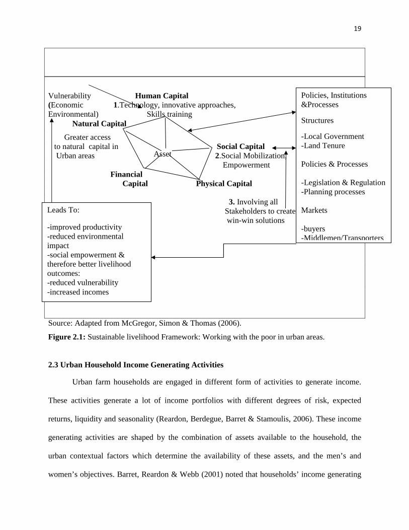
The framework below considers the causes of vulnerability of the poor, their assets and
the policies, processes and institutions that affect their use of assets. These combine to produce a
wide range of ways in which urban farm household construct their livelihood (see fig. 1). The
distorted shape of the assets pentagon in figure 1 below indicates the relative reliance on natural
resources of urban farm households and their access to financial or physical assets. The three
points (numbered) are actions that could help improve the asset base of the poor and change the
policy environment to be more pro-poor to improve wellbeing (as shown in the bottom left box).
19
Vulnerability Human Capital (Economic 1.Technology, innovative approaches, Environmental) Skills training
Natural Capital
Greater access to natural capital in Social Capital Urban areas 2.Social Mobilization,
Empowerment Financial Capital Physical Capital 3. Involving all Stakeholders to create win-win solutions
Source: Adapted from McGregor, Simon & Thomas (2006).
Figure 2.1: Sustainable livelihood Framework: Working with the poor in urban areas.
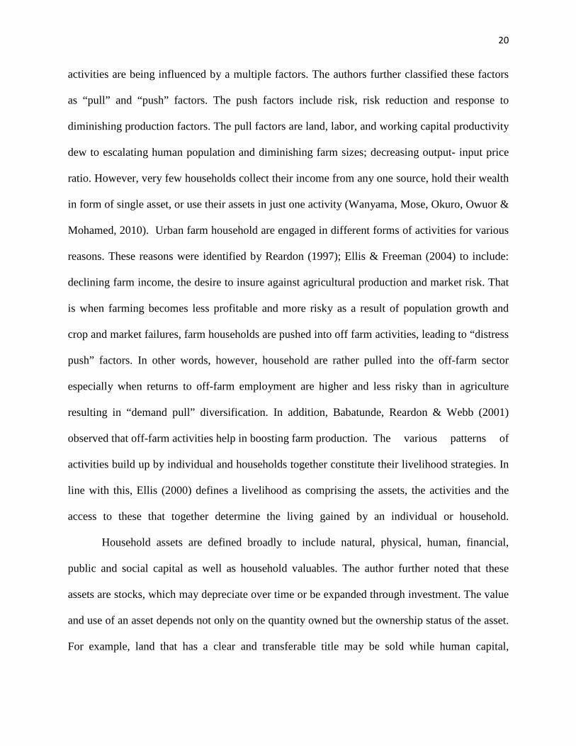
2.3 Urban Household Income Generating Activities
Urban farm households are engaged in different form of activities to generate income.
These activities generate a lot of income portfolios with different degrees of risk, expected
returns, liquidity and seasonality (Reardon, Berdegue, Barret & Stamoulis, 2006). These income
generating activities are shaped by the combination of assets available to the household, the
urban contextual factors which determine the availability of these assets, and the men’s and
women’s objectives. Barret, Reardon & Webb (2001) noted that households’ income generating
Asset
Policies, Institutions &Processes
Structures
-Local Government -Land Tenure Policies & Processes -Legislation & Regulation -Planning processes Markets -buyers -Middlemen/Transporters
Leads To:
-improved productivity -reduced environmental impact -social empowerment & therefore better livelihood outcomes: -reduced vulnerability -increased incomes
20
activities are being influenced by a multiple factors. The authors further classified these factors
as “pull” and “push” factors. The push factors include risk, risk reduction and response to
diminishing production factors. The pull factors are land, labor, and working capital productivity
dew to escalating human population and diminishing farm sizes; decreasing output- input price
ratio. However, very few households collect their income from any one source, hold their wealth
in form of single asset, or use their assets in just one activity (Wanyama, Mose, Okuro, Owuor &
Mohamed, 2010). Urban farm household are engaged in different forms of activities for various
reasons. These reasons were identified by Reardon (1997); Ellis & Freeman (2004) to include:
declining farm income, the desire to insure against agricultural production and market risk. That
is when farming becomes less profitable and more risky as a result of population growth and
crop and market failures, farm households are pushed into off farm activities, leading to “distress
push” factors. In other words, however, household are rather pulled into the off-farm sector
especially when returns to off-farm employment are higher and less risky than in agriculture
resulting in “demand pull” diversification. In addition, Babatunde, Reardon & Webb (2001)
observed that off-farm activities help in boosting farm production. The various patterns of
activities build up by individual and households together constitute their livelihood strategies. In
line with this, Ellis (2000) defines a livelihood as comprising the assets, the activities and the
access to these that together determine the living gained by an individual or household.
Household assets are defined broadly to include natural, physical, human, financial,
public and social capital as well as household valuables. The author further noted that these
assets are stocks, which may depreciate over time or be expanded through investment. The value
and use of an asset depends not only on the quantity owned but the ownership status of the asset.
For example, land that has a clear and transferable title may be sold while human capital,
21
although clearly owned, cannot be transferred. Many urban households’ income generating
strategies integrate rural and peri-urban activities. Many poor urban households are
opportunistic, diversifying their sources of income and drawing, where possible, on a portfolio of
activities (such as formal waged employment, informal trading and service activities). Clearly
the activities undertaken by poor households will in part be determined by the assets available to
households’ members. Chambers (1997) also stresses the importance of the poor diversifying
their income as a broad survival strategy, distinguishing between full time employees with one
main source of livelihoods (‘hedgehogs’), and poor people with a wide portfolio of activities
(‘foxes’). ‘Fox’ households undertake many different activities and strategies. However, it
should be noted that many urban farm households are involved in many income generating
activities out of necessity rather than choice. Meikle, Ramasut & Walker (2001) distinguishes
between short term strategies, often adopted out of necessity as strategies aim at reducing
expenditure and long term strategies aiming to invest in future capacity to build livelihoods. In
this light, it will be wrong to assume that parents who take their children out of school as an
immediate response to a financial household crises do not attribute value to education in the long
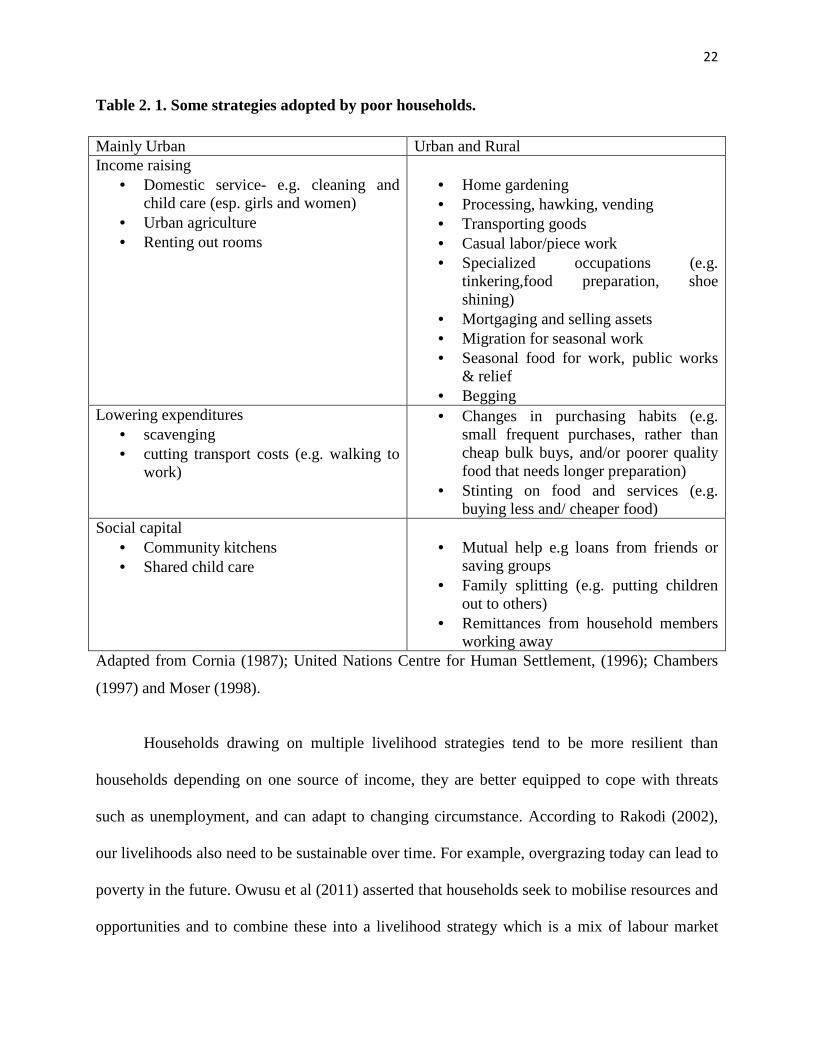
term. Some of the strategies adapted by the poor households are shown in table 2.2 below
22
Table 2. 1. Some strategies adopted by poor households.
Mainly Urban Urban and Rural Income raising
• Domestic service- e.g. cleaning and child care (esp. girls and women)
• Urban agriculture • Renting out rooms
• Home gardening • Processing, hawking, vending • Transporting goods • Casual labor/piece work • Specialized occupations (e.g.
tinkering,food preparation, shoe shining)
• Mortgaging and selling assets • Migration for seasonal work • Seasonal food for work, public works
& relief • Begging
Lowering expenditures • scavenging • cutting transport costs (e.g. walking to
work)
• Changes in purchasing habits (e.g. small frequent purchases, rather than cheap bulk buys, and/or poorer quality food that needs longer preparation)
• Stinting on food and services (e.g. buying less and/ cheaper food)
Social capital • Community kitchens • Shared child care
• Mutual help e.g loans from friends or
saving groups • Family splitting (e.g. putting children
out to others) • Remittances from household members
working away Adapted from Cornia (1987); United Nations Centre for Human Settlement, (1996); Chambers
(1997) and Moser (1998).
Households drawing on multiple livelihood strategies tend to be more resilient than
households depending on one source of income, they are better equipped to cope with threats
such as unemployment, and can adapt to changing circumstance. According to Rakodi (2002),
our livelihoods also need to be sustainable over time. For example, overgrazing today can lead to
poverty in the future. Owusu et al (2011) asserted that households seek to mobilise resources and
opportunities and to combine these into a livelihood strategy which is a mix of labour market
23
involvement; savings; borrowing and investment; productive and reproductive activities; income;
labour and asset pooling; and social networking. Rakodi (2002) argued that households and
individuals adjust the mix according to their own circumstances (age, life-cycle stage,
educational level, tasks) and the changing context in which they live. They further noted that
economic activities form the basis of a household strategy. To these may be added migration
movements, maintenance of ties with rural areas, urban food production, decisions about access
to services such as education and housing, and participation in social networks. Rakodi (2002)
observed that only a few households in poor countries can support themselves through one
business activity (farming or non-farming) or full-time wage employment. Given the inadequate
capital and skills, a poor person's capacity for developing an enterprise with ample profit margins
is limited and, in any case, the risk of relying on a single business is too great. Wages have often
fallen below the minimum required to support a family, as recession and structural adjustment
policies have bitten.
2.4 Asset and Classification
Being able to access, control, and own productive assets such as land, labor, finance, and
social capital enable people to create stable and productive lives (Meinzen et al, 2011).
According to Lerman & McKernan (2008), assets are rights or claims related to property, both
tangible (financial and physical assets) and intangible (e.g., human capital). They are a stock of
resources that can be converted into a flow of income, and provide individuals and families with
security and with the capacity to increase their living standards. To achieve these purposes,
people save and invest in financial, physical, and human capital assets.
Reardon & Vosti (1995) differentiates natural, human, on-farm physical, off-farm
physical, and community owned resources. Barret & Reardon (2000) distinguished between
24
productive and non-productive assets. The authors asserted that productive assets are inputs used
in the productive process and therefore generate income indirectly via the activities. In contrast,
non-productive assets generate income indirectly through transfers of capital gains.
Deere & Doss (2006), in their study noted that productive assets can generate products or
services that can be consumed or sold to generate income. Assets are also stores of wealth that
can increase (or decrease) in value. Assets can act as collateral and facilitate access to credit and
financial services as well as increase social status. Flexibility of assets to serve multiple
functions provides both security through emergencies and opportunities in periods of growth.
Narayan, Petal, Schafft, Rademacher & Koch-Schulte (2000), in their study “voices of
the poor,” observed that “the poor rarely speak of income, but focus instead on managing assets
(physical, human, social and environmental) as a way to cope with their vulnerability.” They
further observed that access to, control over, and ownership of assets including land and
livestock, homes and equipment, and other resources enable people to create stable and
productive lives. Increasing the nexus of control over assets also potentially enables more
permanent pathways out of poverty compared to measures that aim to increase incomes or
consumption alone.
2.4.1 Why Assets are important
In describing why assets are important, it is useful to begin by distinguishing income
from assets. Incomes are flows of resources. They are what people receive as a return on their
labor or use of their capital, or as a public program transfer. Most income is spent on current
consumption. Assets are stocks of resources. They are what people accumulate and hold over
time. Assets provide for future consumption and are a source of security against contingencies.
25
As investments, they also generate returns that generally increase aggregate lifetime
consumption and improve a household’s well-being over an extended time horizon.
The dimensions of poverty, and its relative distribution among different social classes, are
significantly different when approached from an assets perspective, as opposed to an income
perspective. Those with a low stock of resources to draw on in times of need are asset poor. This
asset poverty may leave them vulnerable to unexpected economic events and unable to take
advantage of the broad opportunities offered by a prosperous society (Bebbington, 1999). Many
studies have found that the rate of asset poverty exceeds the poverty rate as calculated by the
traditional measure, which is based on an income standard. Many poor urban farm households
have little financial cushion to sustain them in the event of crop failure, job loss, illness, or other
income shortfall. Also, social and economic development of these households may be limited by
a lack of investment in education, homes, businesses, or other assets.
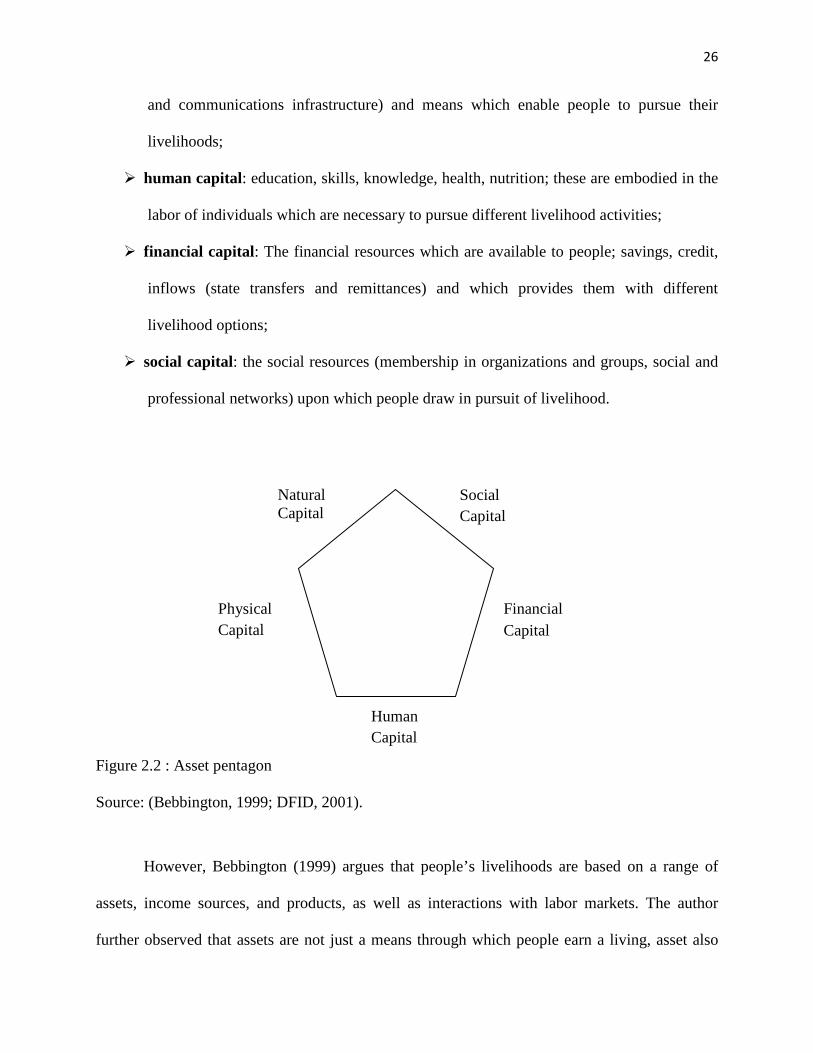
2.4.2 Classification of Assets
Households and individuals hold and invest in different types of assets, including tangible
assets such as land, livestock, and machinery, as well as intangible assets such as education and
social relationships. These different forms of asset holdings have been categorized by
Bebbington (1999); and DFID 2001) in their separate studies as shown in the asset pentagon in
figure 2.2 below:
� natural resource capital: The natural resource stock from which resources flows useful
for livelihoods are derived (e.g land, water, trees, genetic resources, soil fertility);
� physical capital: The basic infrastructures (agricultural and business equipment, houses,
consumer durables, vehicles and transportation, water supply and sanitation facilities,
26
and communications infrastructure) and means which enable people to pursue their
livelihoods;
� human capital: education, skills, knowledge, health, nutrition; these are embodied in the
labor of individuals which are necessary to pursue different livelihood activities;
� financial capital: The financial resources which are available to people; savings, credit,
inflows (state transfers and remittances) and which provides them with different
livelihood options;
� social capital: the social resources (membership in organizations and groups, social and
professional networks) upon which people draw in pursuit of livelihood.
Figure 2.2 : Asset pentagon
Source: (Bebbington, 1999; DFID, 2001).
However, Bebbington (1999) argues that people’s livelihoods are based on a range of
assets, income sources, and products, as well as interactions with labor markets. The author
further observed that assets are not just a means through which people earn a living, asset also
Natural Capital
Human Capital
Physical Capital
Financial Capital
Social Capital
27
give meaning to people’s lives as well as giving individuals the capability to be and to act.
Bebbington’s framework of Capitals and Capabilities treats assets as “vehicles for instrumental
action (making a living), hermeneutic action (living meaningful) and emancipatory action
(challenging the structures under which one makes a living)” (Bebbington, 1999).
2.5 Households Asset Utilization
Household assets are broadly defined to include natural, physical, human, financial and
social capital as well as household valuables (Winters, Davis & Corral 2001). The value and use
of asset depend not only on the quantity owned but also on the ownership status of the asset. For
instance, land has a clear and transferable title and may be sold while human capital, although
clearly owned cannot be transferred. Assets such as literacy and numeracy of household
members, can potentially be used in a number of productive activities while other, such as farm
machinery tend to be coupled with particular activities. Winters, Davis & Corral 2001, also
observed that in some cases such coupling may be products of specialization and can lead to
higher returns to the assets. Based on access to a set of assets, household allocate labor to
different activities to produce outcomes such as income, food security, and investment spending.
The allocation of labor to a particular activity may be short-run response to make-up income
deficit due to economic shock or to obtain liquidity for investment, may be an active attempts to
manage risk involving in different income generating activities, or may be part of a long term
strategy to improve household wellbeing. For this reason at a given point in time household may
get involved in different income generating activities.
Individual within the household may own asset used in different income generating
activities. However, there is now substantial evidence to contradict the still-common assumption
made in economics (and many development projects) that households are groups of individuals
28
who have the same preferences and fully pool their resources. This unitary model has been
rejected in both developed and developing countries, with important implications for policy
(Strauss & Thomas, 1995; Haddad, Ruel & Garret, 1997; Behrman, 1997). An alternative, the
collective model, allows for differences of opinion regarding economic and other decisions
among household members on asset utilization. Most authors (Manser & Brown 1980; McElroy
& Horney, 1981) opined that under the collective model, when there is a disagreement, its
resolution may depend on the bargaining power of individuals within the household. One of the
determinants of the bargaining power of individuals is the ownership and the nexus of control
over assets. Haddad, Ruel & Garret, (1997), in their view, observed that within households,
assets are not always pooled, but rather can be held individually by men, women, and children
who within a household has access to which resources and for what purposes is conditioned both
by the broader socio-cultural context as well as by intra-household allocation rules.
Some household members may contribute more asset than others in terms of income
generation. Empirical evidence shows that women contribute more labor inputs in farming than
men, but men are believed to play the dominant role, and hence income distribution among
household members is erroneously skewed in favor of men (Okorji, 1988).
Different types of assets may also have different implications for bargaining power or
well-being within the household. In societies as diverse as Ethiopia and Indonesia, assets that
women bring to marriage are associated with what they can take upon divorce and their
bargaining power within the household (Fafchamps & Quisumbing, 2002; Thomas, Frankenberg,
& Contreras 2002). However, Panda & Agarwal (2005) observed that in India, ownership of a
house is associated with lower incidence of domestic violence against women. However, intra-
household asset allocation rules is not in the scope of this study.
29
2.6 Linking Asset, Activity Choice and Income: Conceptual approach
Conceptual framework for research purposes is a schematic description and illustration of
the causative mechanisms and relationship deducible from the research problems (Eboh, 2009).
Conceptual framework depicts a schema providing structural meaning and linkages among major
concepts or variables in a phenomena being investigated, their interdependence and relationship
with each other.
However, several forces influence the households’ decision to participate in different
income generating activities. The decision to participate in a certain activity is triggered by the
reward offered, risks associated with the activity and households’ capacity, which is determined
by the assets endowment (Barret, Reardon & Webb, 2001). The conceptual framework of this
study is built on two approaches in the literature linking income and activities: the livelihood
approach and the assets-activities-incomes approach.
There exists some variation in the definition of a livelihood in the literature. This study
earlier adopted the definition by Ellis (2000). As livelihood and income are not synonymous,
they are nevertheless inseparably connected, because income “at a given point in time is the most
direct and measurable outcome of the livelihood process” (Ellis, 2000). The livelihood approach
as defined earlier emphasizes the role of the household’s resources as determinants of activities
and highlights the link between assets, activities and incomes. Moreover, it stresses the
multiplicity of activities households are engaged in. A review of empirical studies on average
shares of income on urban farm households in Africa participating in urban agriculture (Zezza &
Tasciotti, 2010) shows their importance for urban farm households. The authors noted that on the
average, between 18% and 24% of all urban households in African countries sampled,
agricultural activities constitutes 30% of total income or more.
Another approach linking assets, activities and incomes was developed by Barrett &
30
Reardon (2000). The authors, who had a production function in mind, maintained that assets
correspond to the factors of production and incomes to the outputs of production. Activities are
the ex ante production flows of asset services. In contrast to the livelihood approach they
highlight the role of prices in the income generating process. They also point out that “it is
crucial to note that the goods and services produced by activities need to be valued by prices,
formed by markets at meso and macro levels, and in order to obtained the measured outcomes
called incomes” (Barrett & Reardon, 2000). However, more emphasis will be given to factors
mediating the use of assets. This framework has been adopted by several authors including;
Oseni & Winter (2009) in evaluating the effect of rural non-farm income on agricultural crop
production in Nigeria. Babatunde, Reardon & Webb (2010), in determining the effects of
participation in off-farm employment among small-holder farming households in Kwara State,
Nigeria, used a similar approach. Also, Babatunde & Quaim (2010); Wanyama, Mose, Okuro,
Owuor & Mohammed (2010) and Zeller & Minten (2000) adopted similar approach
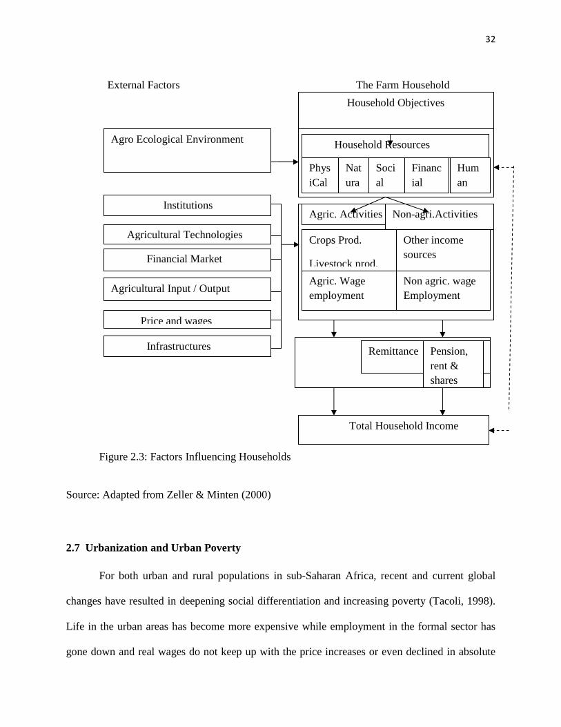
Household is assumed to maximise its utility which is a function of the consumption of
goods and leisure. It is subject to various constraints, such as a cash constraint. According to its
objective, the household allocates its resources to activities subject to factors which are external
to the household (Figure 3). These activities generate outcomes which will meet the objectives.
The activities as well as the income generated have an effect on the stock of resources available
to the house-hold in the future. The total household income is the aggregate measure of the out-
come of all the activities the household is engaged in. Determinants of the production decision
which are external to the household are illustrated on the left hand side of the conceptual
framework. They condition, or as Ellis (2000) calls it, mediate the use of the household’s
resources. The household’s assets are shown on the right hand side, which also stylizes the
31
decision making process of the household. The household is taken as a single decision-making
body. Processes by which resources are allocated among household members, the so-called intra
household resource allocation, are not taken into account due to limitations in time and budget
for data collection. This implies that consequences of policies can only be modeled for the
household as a whole and not for its individual members. Factors external to the household
influencing decision-making are the agro-ecological and socio-economic environment. Main
components of the latter are the access to institutions (such as for agricultural extension and
credit), agricultural technologies, infrastructure and the access to agricultural input and output
markets. These components determine together with development policies the transaction costs
and farm-gate prices of producers and consumers. Figure 2.3 below shows the factors
influencing households
32
External Factors The Farm Household
Figure 2.3: Factors Influencing Households
Source: Adapted from Zeller & Minten (2000)
2.7 Urbanization and Urban Poverty
For both urban and rural populations in sub-Saharan Africa, recent and current global
changes have resulted in deepening social differentiation and increasing poverty (Tacoli, 1998).
Life in the urban areas has become more expensive while employment in the formal sector has
gone down and real wages do not keep up with the price increases or even declined in absolute
Household Objectives
Total Household Income
Household Resources
PhysiCal
Natura
Social
Financial
Human
Agric. Activities Non-agri.Activities
Crops Prod.
Livestock prod.
Other income sources
Agric. Wage employment
Non agric. wage Employment
Remittance
ii
Agro Ecological Environment
Institutions
Agricultural Technologies
Financial Market
Price and wages
Agricultural Input / Output Market
Infrastructures Pension, rent & shares
33
terms (UNDP, 2006). Increases in food prices and service charges and cuts in public expenditure
on health, education and infrastructure have been particularly felt by low-income groups (Tacoli,
2002).
People's responses to (urban) poverty are roughly twofold: first, try to raise or at least
maintain one's income and, secondly, reduce one's expenses. Raising or maintaining one's
income can usually be done by diversification of income sources. Cutting expenses is done on
such services like education and health, on material expenses, as well as on consumption and
dietary pattern. An increasing number of the urban poor in Sub-Saharan Africa have started to
grow some food within the city. This has become an important coping mechanism in the context
of cuts in food subsidies, rises in the cost of living and declines in poor family purchasing power
(Nugent, 2000).
The growth of urban agriculture since the late 1970s is largely understood as a response
to escalating poverty and to rising food prices or shortages which were exacerbated by the
implementation of structural adjustment policies in the 1980s (Drakakis-Smith, 1997; Gefu,
1992; Foeken & Mboganie 2000; Tacoli, 1998). What these changes in the two areas have in
common is the element of risk spreading or risk management: households perform a wide range
of different activities in order to maintain a certain level of living or even to avoid starvation.
However, there is still much debate as to whether urban poverty differs from rural poverty and
whether policies to address the two should focus on different aspects of poverty. In some views,
rural and urban poverty are interrelated and there is a need to consider both urban and rural
poverty together for they have many structural causes in common, e.g. socially constructed
constraints to opportunities (class, gender) and macroeconomic policies. Many point to the
important connections between the two, as household livelihood or survival strategies have both
34
rural and urban components (Satterthwaite, 1995). Baker (1995) and Wratten (1995) illustrate
this point in terms of rural-urban migration, seasonal labor, remittances and family support
networks. Baker (2005) illustrates how urban and rural households adopt a range of
diversification strategies, by having one foot in rural activities and another in urban. This study
addressed how urban farm households used their assets to generate income in other to escape
from poverty.
2.8 Urban agriculture at the household level
Urban farm households face choices in how to allocate their labor and their expenditures
in order to maximize their welfare within a constraint of limited resources. A simple economic
model predicts behavior that would bring the most income into the family. This means family
members jointly choose how to allocate their work time to the most remunerative income-
generating activities over a given time horizon. However, urban farmers are simultaneously
suppliers of labor to agriculture, and producers and consumers of food. This makes the
maximization problem more complex. In order to understand household behavior with respect to
urban agriculture, the existence of other factors that affect income expectations must be brought
into the analysis.
The major economic complications are imperfect labor and land markets in urban areas,
unreliable or sporadic market information available to some urban dwellers, and poor quality or
non-existent markets for inputs, such as credit and fertilizer (Nugent, 2000). The author further
suggested that such conditions imply that a household is likely to have a complicated definition
of welfare that could include diversification of income sources, adaptation to underemployment,
and other goals that will help assure its wellbeing under conditions of uncertainty. Additionally,
35
other factors, such as social expectations, risk perceptions; cultural mores and family gender
relationships also come into play and may be even more important than economic factors.
The behavioral process of urban households facing the decision of whether to farm. On a
microeconomic scale, the decision to engage in urban agriculture will lead to changes in how a
household allocates its time and expenditures. Therefore, from the perspective of suppliers of
labor, households will produce food themselves if the farming activity provides a higher return
(either monetary or in-kind) for the effort expended than other activities. Added to that decision
process is the perspective of households as food consumers. A household will produce its own
food when it is less costly (in terms of time and money) than purchasing food. The effort put into
urban agriculture can be derived from the household’s constrained welfare maximization
problem:
Goal: Maximise household welfare from among employment alternatives, including leisure.
Given: Household resources, such as labour, capital and set of skills; Prices of and access to
foodstuffs and other consumables; Prices of and access to needed inputs, including land; Risks
and uncertainty about markets, policies, and weather.
2.9 Households Vulnerability to Shocks
“Vulnerability refers both to external exposure to shocks, stress and risk (e.g. loss of
income sources, illness, natural disasters, crime) and the inability of people to cope with these
risks without suffering damaging loss. While both the poor and the better off are subject to risks,
the poor are usually less able to cope without suffering from damaging loss (UNDP, 1997)”
Satterthwaite (2007) reasoned that in urban areas, vulnerability is also so much influenced by the
extent and quality of infrastructure and public services, especially for vulnerable populations.
36
Whether or not a farm household is poor is widely recognized as an important, indicator of a
household’s well-being. However, today’s poor may or may not be tomorrow’s poor. Currently
non-poor households, who face a high probability of a large adverse shock, may, on experiencing
the shock, become poor tomorrow. And the currently poor households may include some who
are only transitorily poor as well as other who will continue to be poor (or poorer) in the future.
Urban farm households and communities face the risks of suffering from different types
of shocks. Some shocks affect communities as a whole (these are often referred to as covariate
shocks), such as economic and financial crises and natural disasters. Others affect one or a few
households (idiosyncratic shocks), such as a death or a loss of a job (Ninno & Marini, 2005).
Even though, any household can be affected by those shocks, not all of them have the same
probability of recovering from the consequences of suffering from them. Poor households that
lack the necessary physical and human capital will be less likely to recover from it.
The concept of risk is gaining increasing importance in poverty literature (Azam & Imai,
2012). Sen (1999), observed that “the challenge of development does not only includes the
elimination of persistent and endemic deprivation, but also the removal of vulnerability of
sudden and severe destitution”. This implies that adequate understanding of the risk-poverty
nexus and the way vulnerability affects basic household’s welfare is importance generally for the
design of the developmental policies and poverty reduction in particular. In line with this,
Christiaensen (2004) described vulnerability as an intrinsic aspect of wellbeing, he observed that
“one cannot limit oneself to the person’s actual welfare status today, but must also account for
his prospect for being well in the future. Since being well today does not imply being well
tomorrow. Chaudhuri (2003) construed vulnerability broadly as an ex- ante measure of
wellbeing, reflecting not so much on how well of a household currently is, but what their future
37
prospects are. According to Calvo & Davon (2005), vulnerability can be understood as impact of
risk in the “threat of poverty, measured ex ante, before the veil of uncertainty has been lifted”.
Vulnerability analysis takes into account the occurrence of shock, the level of poverty and the
availability of household’s livelihood assets.
Farm household’s make considerable movement in and out of poverty depending on the
natural, social and economic environments of varying degrees of risks and uncertainty they are
embedded in. Risk may emanate from two broad sources: idiosyncratic shocks; or covariate
shocks. Household’s idiosyncratic shocks are households –specific shocks such as death of the
principal income earner, injury, chronic illness or unemployment/underemployment etc which
are very common in Nigeria and other developing countries. This may be mainly due to the
absence of easy access to medical care, portable drinking water, unhygienic living conditions,
and limited opportunities of diversifying income sources (Azam & Imai, 2012). These
difficulties are compounded by lack of financial intermediation and formal insurance, credit
market imperfections, and weak infrastructural facilities (Gaiha & Imai, 2004).
Covariate shocks i.e community level shocks are natural disasters like floods, cyclones,
droughts or epidemics etc. All these can potentially contribute to high income volatility of
households. Vulnerability is thus a dynamic concept and could be thought of as products of
poverty, household’s exposure to risk and their ability to cope with such risks. However, the
presence of risks can distort household’s inter-temporal allocation behavior, not only for those
who are currently poor, but also for the non-poor who have a high probability of becoming poor
in the future. These distorted behaviors can be economically costly and may propel household
into persistence poverty (Carter & Barrett, 2006). Ajah & Rana (2005) in their view underscored
the need for adequate understanding of the risk- poverty linkage, which they observed could be
38
beneficial in identifying some of the key constraints to poverty reduction binding at micro level.
Identifying who are most vulnerable, as well as what characteristics are correlated with
movements in and out of poverty, can yield a critical insight for policy makers. World Bank
(2000), emphasized that in order to address the objective of poverty reduction, “policies should
not only highlight poverty alleviation interventions to support those who are identified as the
poor ex post, but also the poverty ‘preventions’ to help those who are poor ex ante, that is,
prevent those who are vulnerable to shocks not to fall into poverty. These observations gave birth
to the World Bank’s risk management which highlights three types of risk management
strategies: Prevention, Mitigation and Coping (Holzmann & Jorgensen, 2000).
2.9.1 Prevention Strategies: These are strategies that are implemented before a risk event
occurs. Reducing the probability of an adverse risk increases people’s expected income and
reduces income variance, and both of these effects increase welfare. There are many possible
strategies for preventing or reducing the occurrence of risks, many of which fall outside of social
protection, such as sound macroeconomic policies, environmental policies, and investments in
education. Preventive social protection interventions typically form part of measures designed to
reduce risks in the labor market, notably the risk of unemployment, under-employment, or low
wages due to inappropriate skills or malfunctioning labor markets.
2.9.2 Mitigation Strategies: As with prevention strategies, mitigation strategies aim to address
the risk before it occurs. Whereas preventive strategies reduce the probability of the risk
occurring, mitigation strategies help individuals to reduce the impact of a future risk event
through pooling over assets, individuals, and over time. For example, a household might invest
39
in a variety of different assets that yield returns at different times (for example, two kinds of
crops that can be harvested in different seasons), which would reduce the variability of the
household’s income flow. Another mitigation strategy is for households that face largely
uncorrelated risks to “pool”
them through formal and informal insurance mechanisms.
2.9.3 Coping Strategies: These are strategies designed to relieve the impact of the risk once it
has occurred. The main forms of coping consist of individual dissaving, borrowing, or relying on
public or private transfers. The government has an important role to play in helping people to
cope (for example, when individuals or households have not been able to accumulate enough
assets to handle repeated or catastrophic risks). The smallest income loss would make these
people destitute and virtually unable to recover.
2.9.4 Quantifying vulnerability
Hoddinot & Quisumbing (2003) identified three different methodologies used to assess
vulnerability, these include: Vulnerability as uninsured Exposure to Risk (VER), Vulnerability as
low Expected Utility (VEU) and Vulnerability as Expected Poverty (VEP). All the three methods
construct a measure of welfare of the farm households.
2.9.5 Vulnerability as Uninsured Exposure to Risk (VER)
This method is based on ex post facto assessment of the extent to which a negative shock
causes welfare loss (Hoddinot & Quisumbing, 2003) the impact of shocks is assessed using panel
data to quantify the change in induced consumption.
40
2.9.6 Vulnerability as a Low Expected Utility (VEU)
VEU focuses on the magnitude of the difference in welfare/utility associated with a
certainty equivalent level of welfare (a benchmark) and the household’s own expected
welfare/utility. Under this method, Ligon & Schechter (2003) defined vulnerability as the
difference between utility derived from some level of consumption at and above, which the
household would not be considered vulnerable. The limitation of VER and VEU methods is that,
in the absence of panel data, estimates of impacts, especially from cross sectional data are often
biased and thus inconclusive (Skoufias, 2003).
2.9.7 Vulnerability as Expected Poverty (VEP)
VEP focuses on the likelihood that well-being will be below the benchmark in the future,
under this framework, a farmer’s vulnerability is considered as the probability of that farmer
becoming poor in the future if currently not poor or the prospect of that farmer continuing to be
poor if currently poor (Christiaensen & Subbarao, 2004). It is argued that pre-existing conditions
and forces influences the magnitude and the ability of farm households or communities to reduce
their vulnerability to shocks. Hence, under this scenario, vulnerability is seen as expected
poverty, with consumption or income being used as the welfare indicator. In this conception, the
vulnerability is measured by estimating the probability that a given shock, or set of shocks,
moves consumption of an individual/household below a given minimum level (for example a
consumption poverty line) or forces the consumption level to stay below the given minimum
requirement if it is already below that level (Chaudhuri, Jalan & Suryahadi, 2002). In this case,
vulnerability can be measured using the cross sectional data unlike the other methods that require
panel data. Both measures have much in common. They differ in
41
1)Their definition of well-being
2)Their treatment of states of the world above the benchmark.
2.10 Theoretical Framework
Several forces influence the households’ decision to participate in different income
generating activities. Qasim, (2012) asserted that the farm household behavior is influenced by
several natural markets and social uncertainties in developing countries. This has raised some
complexities in terms of understanding their production decisions. According to (Corral &
Reardon, 2001), farm households’ decision to participate in a certain activity is triggered by the
rewards offered, risks associated with the activity and households’ capacity which is determined
by asset endowment, and this explains why not all household have the same opportunities to
participate in different activities. The main theories behind this study are utility theory,
sustainability theory and theories considering risk-averse farmers.
2.10.1 Utility Theory
Utility theory is concerned with people’s choice and decisions. It is concerned also with
preferences and with judgements of preferability, worth, value, goodness or any of a number of
similar concepts (Fishburn, 1968). This theory provides a methodological framework for the
evaluation of alternative choices made by individual, firms and organisations. Utility refers to the
satisfactions that each choice provides to the decision makers. Thus, this theory assumes that any
decision is made on the basis of the utility maximization principles according to which the best
choice is the one that provides the highest utility (satisfaction) to the decision makers.
Utility theory is often used to explain the behaviour of individual consumers. In this case,
42
urban farmer plays the role of the decision maker that must decide which income generating
activities to participate to secure the highest possible level of total utility subject to his or her
available asset and other factors. The traditional framework of the utility theory has been
extended over the past three decades to multi-attribute case, in which decisions are taken by
multiple criteria. In all cases the utility that the decision makers that is, farmers get from
selecting an income generating activity is measure by a utility function U, which is a
mathematical representation of the decision makers (farmers) system of preferences such that: U
(x1) > U (x2), where choice of an income generating activity x1 is preferred over choice x2 or Ux1
= Ux2, where choice x1 is indifferent from choice x2, that is both choices are equally preferred.
Also, preferences are described by their utility function or payoff function. This is an ordinal
number an individual assigns over the available actions, such as:
U (ai) > U (aj)
The individual's preferences are then expressed as the relation between these ordinal
assignments (Allingham, 2002). For example, if a farmer prefers owning a farm over working as
wage labourer and as a wage labourer over remittance earnings, his preferences would have the
relation:
U (Owned farm) > U (wage labourer) > U (remittance earnings).
In this case, it could be inferred that owning a farm is prefer over remittance earnings.
The income generating activities adopted by the farmers was modelled into MNL function to
determine the socio-economic factors that influence the income generating activities among
urban farm households.
43
2.10.2 Sustainability theory
Theories of sustainability attempt to prioritize and integrate social responses to environmental
and cultural problems. An economic model relates to sustain natural and financial capital; an
ecological model relates to biological diversity and ecological integrity; a political model relates
to social systems that realize human dignity. Religion has entered the debate with symbolic,
critical, and motivational resources for cultural change. Economic models propose to sustain
opportunity, usually in the form of capital. According to the classic definition formulated by the
economist Solow (1991), “we should think of sustainability as an investment problem, in which
we must use returns from the use of natural resources to create new opportunities of equal or
greater value”. The theoretical basis of sustainability theory is the forms of progress that meet the
needs of the present without compromising the ability of future generations to meet their needs
(Shahan, 2009). One of the major concerns of economist is how to make efficient use of scarce
natural resources with alternative uses so as to ensure sustainability and improved environmental
quality for man (Hoffman & Ashwell, 2001). Sustainability as regards natural resources such as
land and its deposits, forests, air and water bodies means a balanced use of these resources over a
long period of time without impairing the fundamental ability of the natural resource base to
support future generation. An environmentally sustainable system must maintain a stable
resource base, avoiding over-exploitation of renewable resource systems or environmental sink
functions, and depleting non-renewable resources only to the extent that investment is made in
adequate substitutes.
Sustainability has become a key concept to solving global resource and environmental
issues (McGee, 2006) most especially in the management of natural resources in an urbanizing
world (fast growing urban population). Sustainable agriculture according to Olowookere (2010)
44
is the ability of farmers to produce food in such a way that the environment and surrounding
ecosystem, is unaffected by their agricultural activities. This study assessed how urban farm
household utilize the available natural resources (assets) in their income generating activities.
2.10.3 Theories considering Risk-averse Farmers
According to Dasgupta (1993), seeking to insure household members against hunger and
poverty is of great importance to any farm family in a developing country. The risk behavior of
farm household (engaging in different income generating activities) is determined not only by
individual preferences but also by the availability of institutions that facilitate risk bearing
(Rounasset, 1976). Where institutional arrangements provide imperfect insurance, household will
self-protect themselves by exercising caution in their production decisions (Morduch, 1995). All
these factors formulate farm households’ production choices and explain why vulnerable farmers
are often observed to sacrifice expected profits for greater self-protection.
Ellis (1992) asserted that farm households always operate under risk and uncertainty
induced by natural hazards (weather, pests, diseases, and natural disasters), market fluctuations
and social uncertainty (insecurity associated with control over resources such as land tenure and
state interventions, and war). These conditions pose risks to farm production and make farmers
cautious in their decision making (Walker & Jodha, 1986). Farmers are generally assumed to
exhibit risk aversion in their decision making. Lipton, (1968) who criticized profit maximization
approach showed that the existence of uncertainty and risk eroded theoretical basis of profit-
maximizing model. He argued that small-scale farmers are risk averse, because they have to
secure their household needs from their current activity or face starvation.
45
There are two ways of conceptualizing the farm households’ risk aversion, the standard
expected utility theory and the disaster avoidance approach. According to the former approach,
farm households make choices from available risky alternatives, based on what appeals most to
their given preferences in relation to outcomes and their beliefs about the probability of
occurrence. This normative approach is based on a set of assumptions and on an implicit
hypothesis that farm household, as decision makers are in fact utility maximizers. Both
household behavior and its revealed attitude towards risk (e.g risk aversion) are reflected in its
utility function. Other things being equal a risk –averse household prefers a smooth income
stream to a fluctuating one. This, in contexts of incomplete capital markets or underdeveloped
institutional arrangements entails a low risk portfolio choice of productive activities (Morduch,
1994).
The disaster avoidance approach assumed that, among risky income sources, farm
households first opt for safety, and that they choose (from different income generating activity)
safe alternatives based on expected utility. These models based on a feasible decision process are
known as safety first models of choice under uncertainty. In this case the decision maker wants
to ensure survival for him or herself and to avoid the risk of his or her income falling below a
certain minimum (subsistence) level (Qasim, 2012). This safety- first criterion can lead the
household into favoring either risky income streams or low risk alternatives. This means there is
no reason to expect that individuals behave in conformity with the expected utility theory at very
low income levels. The disaster avoidance perspective is helpful for describing individual choice
under such conditions (Dasgupta, 1993). The attraction of safety –first approach is that it is a
positive method to capture some specific behavior that can be eliminated from the expected
utility theory near threshold income levels. The safety-first theory does not take actual decision
46
rules as given, as in a “pure behavioural approach”. This theory is an appropriate descriptive
device for a risky choice in low income farm farmers. Utility maximization theory cannot highlight
such problems as extreme poverty, insecurity, and deprivation that characterize farm life in most
parts of the world, the safety –first theory explicitly captures these aspects of farm behavior in
developing economies (Qasim, 2012).
2.11 Analytical Framework
The nature and purpose of study determine the type of analysis to be employed
(Chukwuone, 2009). Also, the choice of techniques depends on a host of factors in particular the
objectives of the study, the availability of data, time and budget (McNally & Othman, 2002).
Different approaches could be used to analyze data. The first step of simple but important
analytical tool used in data analysis is the descriptive statistical tools (McNally & Othman,
2002). These include frequency distributions, percentages, mean, bar charts and standard
deviation. However, any study that requires a detailed analysis of quantitative relations needs a
higher level of analysis other than descriptive statistical tools (Eboh, 2009). In this study, in
addition to descriptive statistical tools, the following specific models were employed. Ordinary
least square (OLS) regression analysis, Multinomial logistic (MNL) regression analysis, Quantile
regression model and Vulnerability index analysis.
2.11.1 Ordinary Least Squares (OLS)
Ordinary least-squares (OLS) regression is a generalized linear modelling technique that
may be used to model a single response variable which has been recorded on at least an interval
scale. The technique may be applied to single or multiple explanatory variables and also
categorical explanatory variables that have been appropriately coded (Hutcheson, 2011).
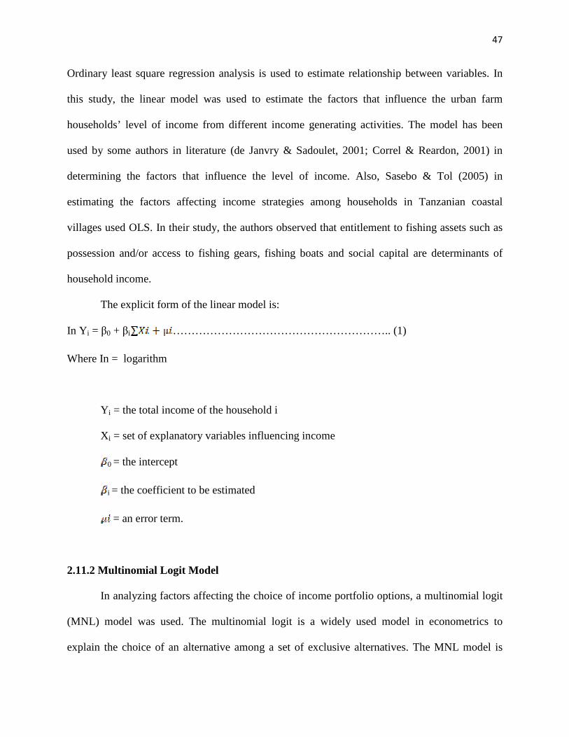
47
Ordinary least square regression analysis is used to estimate relationship between variables. In
this study, the linear model was used to estimate the factors that influence the urban farm
households’ level of income from different income generating activities. The model has been
used by some authors in literature (de Janvry & Sadoulet, 2001; Correl & Reardon, 2001) in
determining the factors that influence the level of income. Also, Sasebo & Tol (2005) in
estimating the factors affecting income strategies among households in Tanzanian coastal
villages used OLS. In their study, the authors observed that entitlement to fishing assets such as
possession and/or access to fishing gears, fishing boats and social capital are determinants of
household income.
The explicit form of the linear model is:
In Yi = β0 + βi ………………………………………………….. (1)
Where In = logarithm
Y i = the total income of the household i
X i = set of explanatory variables influencing income
0 = the intercept
i = the coefficient to be estimated
= an error term.
2.11.2 Multinomial Logit Model
In analyzing factors affecting the choice of income portfolio options, a multinomial logit
(MNL) model was used. The multinomial logit is a widely used model in econometrics to
explain the choice of an alternative among a set of exclusive alternatives. The MNL model is
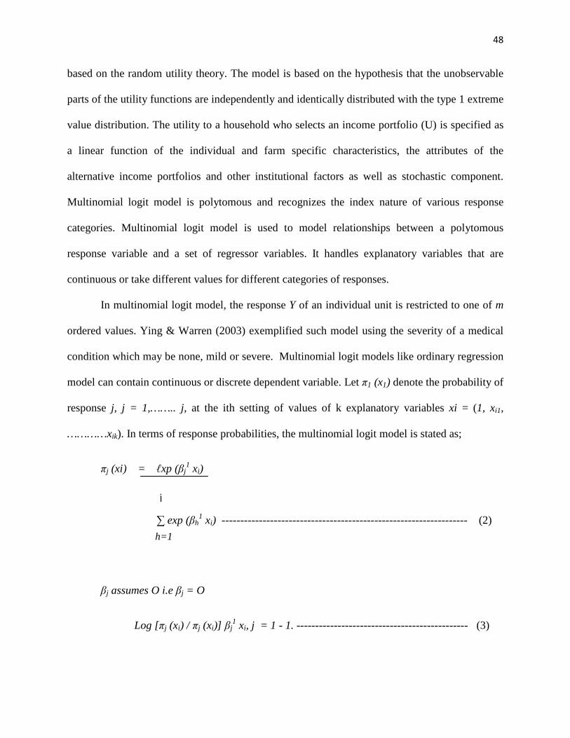
48
based on the random utility theory. The model is based on the hypothesis that the unobservable
parts of the utility functions are independently and identically distributed with the type 1 extreme
value distribution. The utility to a household who selects an income portfolio (U) is specified as
a linear function of the individual and farm specific characteristics, the attributes of the
alternative income portfolios and other institutional factors as well as stochastic component.
Multinomial logit model is polytomous and recognizes the index nature of various response
categories. Multinomial logit model is used to model relationships between a polytomous
response variable and a set of regressor variables. It handles explanatory variables that are
continuous or take different values for different categories of responses.
In multinomial logit model, the response Y of an individual unit is restricted to one of m
ordered values. Ying & Warren (2003) exemplified such model using the severity of a medical
condition which may be none, mild or severe. Multinomial logit models like ordinary regression
model can contain continuous or discrete dependent variable. Let π1 (x1) denote the probability of
response j, j = 1,…….. j, at the ith setting of values of k explanatory variables xi = (1, xi1,
…………xik). In terms of response probabilities, the multinomial logit model is stated as;
πj (xi) = ℓxp (βj1 xi)
∑ exp (βh1 xi) ------------------------------------------------------------------ (2)
βj assumes O i.e βj = O
Log [πj (xi) / πj (xi)] βj1 xi, j = 1 - 1. ---------------------------------------------- (3)
j
h=1
49
Multinomial logit model is one of the most widely used models for ordinal response data.
Several empirical studies in which the dependent variable has to be measured in an ordinal
categorical manner and in which multinomial logit model has been employed include study
conducted by Stratton, O’toole & Wetzel (2003) to estimate the attrition that distinguishes
between stop out and dropout behaviour. The respondents in the study were made to face three
choices; continuous enrolment =1, short term enrolment =2 and long–term dropout=3. Also
Pablo & Miguel (2005) on the factors influencing the adoption of environmental technologies in
the pulp and paper sector in Spain employed multinomial logit model. In their study, three sets of
interrelated factors influencing the widespread adoption of these technologies were considered;
factors of external to the farm, characteristics of the environmental technologies, and internal
characteristics / conditions of the potential adopters. Chukwuone (2009) carried out a study on
analysis of conservation and utilization of Non-wood forest products in Southern Nigeria. The
author used multinomial logistic regression to determine the socio-economic characteristics of
respondent that determine the odds of a household being in one of the categories of production of
non – wood forest product species; production of non-wood forest product was categories into
four. Okon, Enete & Amusa (2012) in estimating the socio economic factors that influenced
urban farmers’ enterprise choice decisions in Uyo Metropolis employed multinomial logit. Also,
Okorji, Okon & Nwankwo (2012) in estimating factors influencing choice of irrigation
techniques among dry season vegetable farmers in Anambra State, Nigeria employed
multinomial logit model.
The MNL category is modelled as a function of individual specific characteristics x that
affect the category associated with each choice differently; Hence, Uji = Xi α j + ℓji .................(4)
where; j = denotes the category,
50
i = denotes the individual.
In this study MNL was used to estimate the socio economic factors that influenced the urban
farm households’ choice of income generating activities. The socio-economic characteristics of
the farm household constitute the explanatory variables for this study. These variables are clearly
defined under section 3.4 of the methodology. By implication, after estimating the parameters,
one can predict the probability that a sampled farm household either with a specified set of socio-
economic characteristics may choose from the category of income generating activities.
2.11.3 Quantile Regression
Quantile regression is a way to estimate the conditional quantiles of a response variable
distribution in the linear model that provides a more complete view of possible causal
relationships between variables. Ordinary least squares (OLS) regression analyses would give an
incomplete picture of the relationships between variables. This is especially problematic for
regression models with heterogeneous variances, which are common in Agriculture. A regression
model with heterogeneous variances implies that there is not a single rate of change that
characterizes changes in the probability distributions. Focusing exclusively on changes in the
means may underestimate, overestimate, or fail to distinguish real nonzero changes in
heterogeneous distributions (Terrell, Cade, Carpenter & Thompson, 1996; Cade, Terrel, &
Schroeder, 1999). As a consequence, there may be a weak or no predictive relationship between
the mean of the response variable (y) distribution and the measured predictive factors (X) as in
ordinary least squares. Yet there may be stronger, useful predictive relationships with other parts
of the response variable distribution. This study prefers quantile regression estimates to ordinary
least squares because OLS regression models the relationship between one or more covariates X
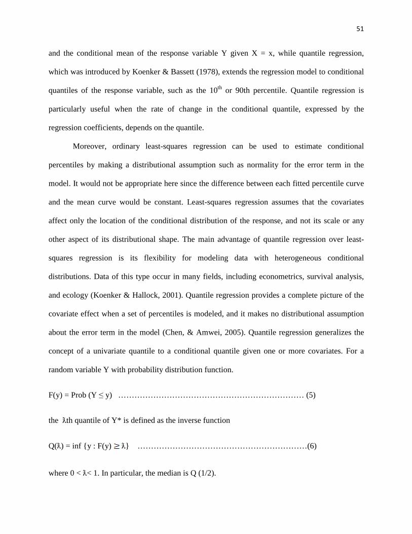
51
and the conditional mean of the response variable Y given X = x, while quantile regression,
which was introduced by Koenker & Bassett (1978), extends the regression model to conditional
quantiles of the response variable, such as the 10th or 90th percentile. Quantile regression is
particularly useful when the rate of change in the conditional quantile, expressed by the
regression coefficients, depends on the quantile.
Moreover, ordinary least-squares regression can be used to estimate conditional
percentiles by making a distributional assumption such as normality for the error term in the
model. It would not be appropriate here since the difference between each fitted percentile curve
and the mean curve would be constant. Least-squares regression assumes that the covariates
affect only the location of the conditional distribution of the response, and not its scale or any
other aspect of its distributional shape. The main advantage of quantile regression over least-
squares regression is its flexibility for modeling data with heterogeneous conditional
distributions. Data of this type occur in many fields, including econometrics, survival analysis,
and ecology (Koenker & Hallock, 2001). Quantile regression provides a complete picture of the
covariate effect when a set of percentiles is modeled, and it makes no distributional assumption
about the error term in the model (Chen, & Amwei, 2005). Quantile regression generalizes the
concept of a univariate quantile to a conditional quantile given one or more covariates. For a
random variable Y with probability distribution function.
F(y) = Prob (Y ≤ y) …………………………………………………………… (5)
the ƛth quantile of Y* is defined as the inverse function
Q(ƛ) = inf {y : F(y) ƛ} ………………………………………………………(6)
where 0 < ƛ< 1. In particular, the median is Q (1/2).
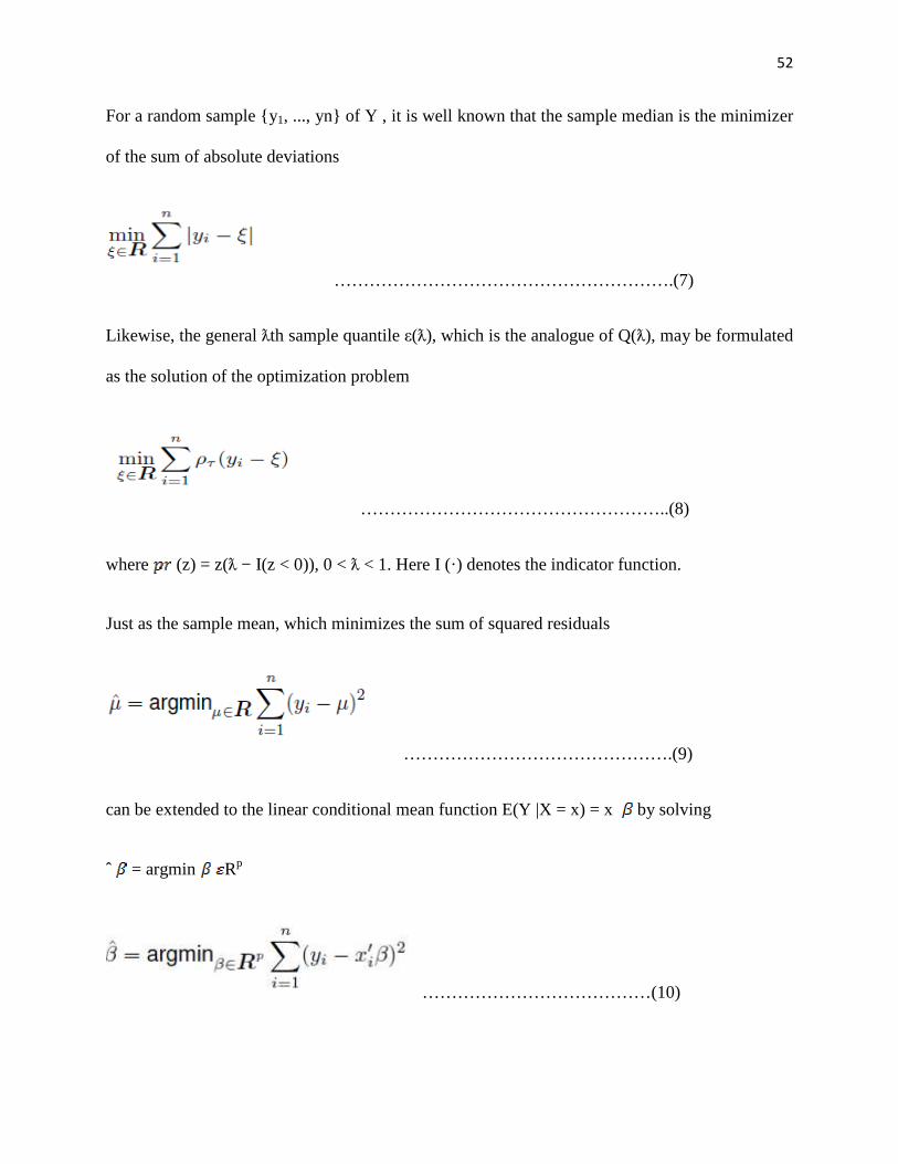
52
For a random sample {y1, ..., yn} of Y , it is well known that the sample median is the minimizer
of the sum of absolute deviations
………………………………………………….(7)
Likewise, the general ƛth sample quantile ε(ƛ), which is the analogue of Q(ƛ), may be formulated
as the solution of the optimization problem
……………………………………………..(8)
where (z) = z(ƛ − I(z < 0)), 0 < ƛ < 1. Here I (·) denotes the indicator function.
Just as the sample mean, which minimizes the sum of squared residuals
……………………………………….(9)
can be extended to the linear conditional mean function E(Y |X = x) = x by solving
ˆ = argmin Rp
…………………………………(10)
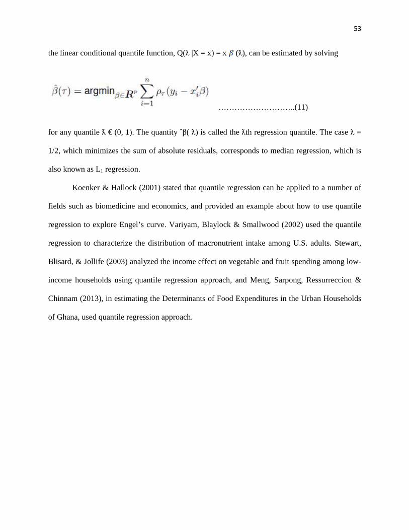
53
the linear conditional quantile function, Q(ƛ |X = x) = x (ƛ), can be estimated by solving
………………………..(11)
for any quantile ƛ € (0, 1). The quantity ˆβ( ƛ) is called the ƛth regression quantile. The case ƛ =
1/2, which minimizes the sum of absolute residuals, corresponds to median regression, which is
also known as L1 regression.
Koenker & Hallock (2001) stated that quantile regression can be applied to a number of
fields such as biomedicine and economics, and provided an example about how to use quantile
regression to explore Engel’s curve. Variyam, Blaylock & Smallwood (2002) used the quantile
regression to characterize the distribution of macronutrient intake among U.S. adults. Stewart,
Blisard, & Jollife (2003) analyzed the income effect on vegetable and fruit spending among low-
income households using quantile regression approach, and Meng, Sarpong, Ressurreccion &
Chinnam (2013), in estimating the Determinants of Food Expenditures in the Urban Households
of Ghana, used quantile regression approach.
54
CHAPTER THREE METHODOLOGY
3.1 Study area
Nigeria lies between latitudes 40 and 140 N and longitudes 30 and 140 E, covering a land
area of about 92,000km2 with a population of about 150 million people (NPoC, 2006). The study
was carried out in the South-South geopolitical zone of Nigeria, which is strategically located at
the point where the river Niger joins the Atlantic Ocean through the Gulf of Guinea. The South-
South region is made up of six out of the 36 States of the Federal Republic of Nigeria. The six
States are Akwa Ibom, Bayelsa, Cross River, Edo, Delta and Rivers States. The area has a total
population of 21,034,081 people (NPoC, 2006). The South-South which is the core oil producing
area provides the economic mainstay of the country: oil and gas. In addition to oil and gas, the
region equally contributes other key resources, with potential huge opportunities in tourism and
agriculture. It has an average annual rainfall of 1,200 to 2,500mm (NIMET, 2012). The climate
of the area allows for favourable cultivation and extraction of agricultural and forest products
such as palm produce, rubber, cocoa, cassava, yam, plantain, banana, maize, vegetables, timber
etc. Majority of the inhabitants are farmers, practicing farming and other enterprises such as crop
production, livestock breeding, forestry practices, fisheries, aquaculture, agricultural processing
as well as urban commerce and transport business.
3.2 Sampling Procedure This study employed purposive, multistage and simple random sampling techniques in
selecting the respondents. Three (3) out of the six States in the South-South geographical zone
were randomly selected, namely: Akwa Ibom, Cross River and Delta States. Three of the State
55
capitals were purposively selected (namely, Uyo, Calabar and Asaba), since the study is on urban
agriculture. Three additional towns classified as urban from Nigerian living Standard survey
were randomly selected from each of the selected States, namely; Ikot Ekpene, Ikom and Warri
from Akwa Ibom, Cross River and Delta States respectively, making a total of six urban areas.
The selected urban areas were in line with the characteristics and classification of urban areas in
Nigeria, as having a population of more than 20,000 people (UNCHS, 2001). In addition to
population density, there are divisions of labour, inhabitants are from diverse races and culture,
having varieties of food habits, administrative and social amenities, occupational specialization
are very much in common. Lists of urban farmers were obtained from the State Agricultural
Development Programme offices. Eighty households were randomly selected from each of the
three selected State capitals, while twenty households were randomly selected from each of the
additional towns in the State, all in proportion to the population of the cities. This gave a sample
size of three hundred households (100 from each State). However, data from Delta State were
less than 100 due inconsistencies by some respondent in filling/returning of some questionnaires.
After data cleaning, 89 questionnaires were considered appropriate for analysis from Delta State.
This gave effective sample size of 289 respondents.
3.3 Method of Data Collection
Data for this study were obtained mainly from primary sources using structured and
pretested questionnaires administered by the researcher and trained enumerators to cover the
three selected States. Because many households lacked sufficient information to adequately
address all the issues regarding income composition. The study adopted intensive cost route
approach to data collection. That is a weekly expenditure of the participating households was
56
used. This reduced measurement errors which could have arisen from poor memory recall. The
income data were collected using expenditure approach. Data were collected for a period of six
months.
The data focused on the following: household composition and other socio-economic
data of the respondents, namely: the production pattern, income generating activities undertaken
by the respondents, and level of assets, membership of organizations, gender of household heads,
engagement in agricultural/ non agricultural activities, asset utilization, and household
vulnerability to shocks. Broadly, this study disaggregates activities and income into seven
categories: (i) Crop Income; (ii) Livestock Income (iii) Agricultural Wage income including
earnings from supplying wage labour to other farms; (iv) non-agricultural wage income
including income from both formal and informal wage employment (v) other income sources, i.e.
income from owned businesses; (vi) remittance income received from relatives and friends not
presently living in the household; (vii) income from pension, shares and rents. However, the first
three are grouped into agricultural income while the last four are grouped into non- agricultural
income. It should be noted that this study focused on urban households’ involvement in
agriculture rather than strictly urban agricultural activities. Therefore the location of the farm
does not matter.
3.4 Data Analysis
Data collected were analyzed using descriptive and relevant inferential statistics in order
to achieve the specific objectives. Objectives (i) and (ii) were achieved using descriptive
statistics such as percentages, frequencies, bar charts, means and standard deviations. In
objective (ii), household’s asset comprising natural capital (was measured by size of land
57
holdings), physical capital (livestock and other physical asset owned by farm household were
measured by valuation). Human capital was measured by years of formal schooling. Social
capital was measured by membership of an organization. Financial capital was measured by the
accessibility of credit sources. Objective (iii) was actualized using ordinary least square
regression model. Objective (iv) was realized using multinomial logistic regression model
(MNL). Objective (v) was realized using quantile regression model. Vulnerability analysis was
used to achieve objective (vi). Hypotheses (i), (ii) and (iii) were tested using t-test as embedded
in the inferential statistical tools. Hypothesis (iv) was tested using vulnerability index analysis.
Model specification
3.4.1 Ordinary Least Squares (OLS)
To determine the influence of socio-economic factors on household income from each of
the income generating activities, ordinary least square (OLS) method of estimation was used.
Four functional forms (linear, semi-log, double-log and exponential) were specified, the linear
models were chosen as the best fit in all income categories. These models are expressed thus:-
Yi = β0 + β1Х1+ β2Х2 + β3Х3+ β4Х4+ β5Х5 + β6Х6 + β7Х7 + β8Х8 + β9Х9 + µ
Yi = household income from an income generating activity
β0 = intercepts, Х1 – Х9 are vector of the variables influencing income, β1 – β9 vector co-efficient
which was estimated and µ = error term.
Х1 = Age of Household Head (in years),
Х2 = Educational level of household Head (Years of formal schooling),
58
Х3 = household size (Number of household member)
Х4 = Farming Experience (in years)
Х5 = Farm size in ha (area of land own by household),
Х6 = Assets (value of productive asset owned by the household in Naira),
Х7 = Gender of household head (dummy, male =1, otherwise =0),
Х8 = Access to formal or informal credit (dummy, if have access = 1, otherwise = 0),
Х9 = Marital Status (dummy, 1 if married, otherwise = 0),
NB productive assets include farm implements and transport equipments as well as household
appliances such as sewing machines, and refrigerators. Also, incomes from the different income
generating activities are thus: Liv- income = livestock income, CR-income = crop income, Aw-
income = agric wage income, NAW-income = non- agric wage income, OTH-income = income
from other sources , RE-income = Remittance income, and PSR= income from Pension, shares
and rents.
3.4.2: Multinomial Logit model (MNL)
The categorical nature of the dependent variable (choice of participation) in income
generating activities in objective (iv), multinomial logit was used to estimate the influence of
socio-economic characteristics of the respondent on the choice of an income generating activity
in the surveyed area. The choice decision which determines the odds of a particular household
participating in one of the income generating activity listed in section 3.3 above was chosen. The
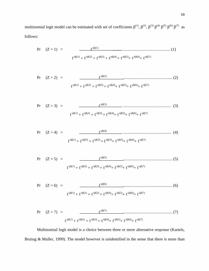
59
multinomial logit model can be estimated with set of coefficients β(1), β(2), β(3) β(4) β(5) β(6) β(7) as
follows:
Pr (Z = 1) = ℓxβ(1) ........................................................ (1)
ℓxβ(1) + ℓxβ(2) + ℓxβ(3) + ℓxβ(4) + ℓxβ(5)+ ℓxβ(6)+ ℓxβ(7)
Pr (Z = 2) = ℓxβ(2) ................................................ (2)
ℓxβ(1) + ℓxβ(2) + ℓxβ(3) + ℓxβ(4)+ ℓxβ(5)+ ℓxβ(6)+ ℓxβ(7)
Pr (Z = 3) = ℓxβ(3) ............................................... (3)
ℓxβ(1) + ℓxβ(2) + ℓxβ(3) + ℓ
xβ(4)+ ℓxβ(5)+ ℓxβ(6)+ ℓxβ(7)
Pr (Z = 4) = ℓxβ(4) ............................................... (4)
ℓxβ(1) + ℓxβ(2) + ℓxβ(3) + ℓ
xβ(3)+ ℓxβ(5)+ ℓxβ(6)+ ℓxβ(7)
Pr (Z = 5) = ℓxβ(5) ................................................ (5)
ℓxβ(1) + ℓxβ(2) + ℓxβ(3) + ℓxβ(4)+ ℓxβ(5)+ ℓxβ(6)+ ℓxβ(7)
Pr (Z = 6) = ℓxβ(6) ................................................ (6)
ℓxβ(1) + ℓxβ(2) + ℓxβ(3) + ℓxβ(4)+ ℓxβ(5)+ ℓxβ(6)+ ℓxβ(7)
Pr (Z = 7) = ℓxβ(7) ................................................ (7)
ℓxβ(1) + ℓxβ(2) + ℓxβ(3) + ℓxβ(4)+ ℓxβ(5)+ ℓxβ(6)+ ℓxβ(7)
Multinomial logit model is a choice between three or more alternative response (Kartels,
Boztug & Muller, 1999). The model however is unidentified in the sense that there is more than
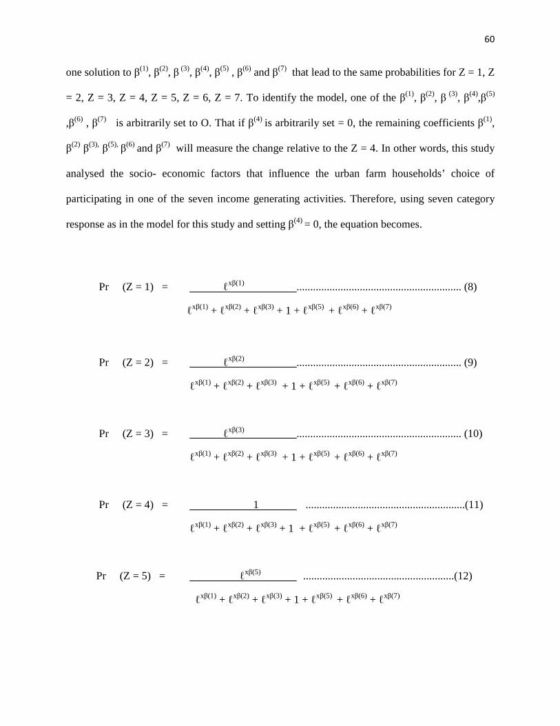
60
one solution to β(1), β(2), β (3), β(4), β(5) , β(6) and β(7) that lead to the same probabilities for Z = 1, Z
= 2, Z = 3, Z = 4, Z = 5, Z = 6, Z = 7. To identify the model, one of the β(1), β(2), β (3), β(4),β(5)
,β(6) , β(7) is arbitrarily set to O. That if β(4) is arbitrarily set = 0, the remaining coefficients β(1),
β(2) β(3), β(5),
β(6) and β(7) will measure the change relative to the Z = 4. In other words, this study
analysed the socio- economic factors that influence the urban farm households’ choice of
participating in one of the seven income generating activities. Therefore, using seven category
response as in the model for this study and setting β(4) = 0, the equation becomes.
Pr (Z = 1) = ℓxβ(1) ............................................................ (8)
ℓxβ(1) + ℓxβ(2) + ℓxβ(3) + 1 + ℓxβ(5) + ℓxβ(6) + ℓxβ(7)
Pr (Z = 2) = ℓxβ(2) ............................................................ (9)
ℓxβ(1) + ℓxβ(2) + ℓxβ(3) + 1 + ℓxβ(5) + ℓxβ(6) + ℓxβ(7)
Pr (Z = 3) = ℓxβ(3) ............................................................ (10)
ℓxβ(1) + ℓxβ(2) + ℓxβ(3) + 1 + ℓxβ(5) + ℓxβ(6) + ℓxβ(7)
Pr (Z = 4) = 1 ..........................................................(11)
ℓxβ(1) + ℓxβ(2) + ℓxβ(3) + 1 + ℓxβ(5) + ℓxβ(6) + ℓxβ(7)
Pr (Z = 5) = ℓxβ(5) .......................................................(12)
ℓxβ(1) + ℓxβ(2) + ℓxβ(3) + 1 + ℓxβ(5) + ℓxβ(6) + ℓxβ(7)
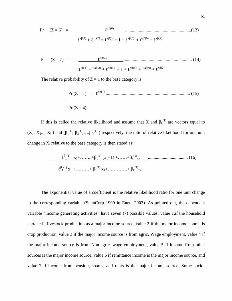
61
Pr (Z = 6) = ℓxβ(6) ..........................................................(13)
ℓxβ(1) + ℓxβ(2) + ℓxβ(3) + 1 + ℓxβ(5) + ℓxβ(6) + ℓxβ(7)
Pr (Z = 7) = ℓxβ(7) ............................................................ (14)
ℓxβ(1) + ℓxβ(2) + ℓxβ(3) + 1 + ℓxβ(5) + ℓxβ(6) + ℓxβ(7)
The relative probability of Z = 1 to the base category is
Pr (Z = 1) = ℓxβ(1) .......................................................................... (15)
Pr (Z = 4)
If this is called the relative likelihood and assume that X and βk(1) are vectors equal to
(X1, X2..., Xn) and (β1(1), β2
(1),….βk(1) ) respectively, the ratio of relative likelihood for one unit
change in Xi relative to the base category is then stated as;
ℓβ1(1) x1+……..+β1
(1) (x1+1) +……+βk(1)
xk ................................... (16)
ℓβ1(1) x1 +………+ β1
(1) x1+………….+ βk(1)
xk.
The exponential value of a coefficient is the relative likelihood ratio for one unit change
in the corresponding variable (StataCorp 1999 in Enete 2003). As pointed out, the dependent
variable “income generating activities” have seven (7) possible values; value 1,if the household
partake in livestock production as a major income source, value 2 if the major income source is
crop production, value 3 if the major income source is from agric. Wage employment, value 4 if
the major income source is from Non-agric. wage employment, value 5 if income from other
sources is the major income source, value 6 if remittance income is the major income source, and
value 7 if income from pension, shares, and rents is the major income source. Some socio-
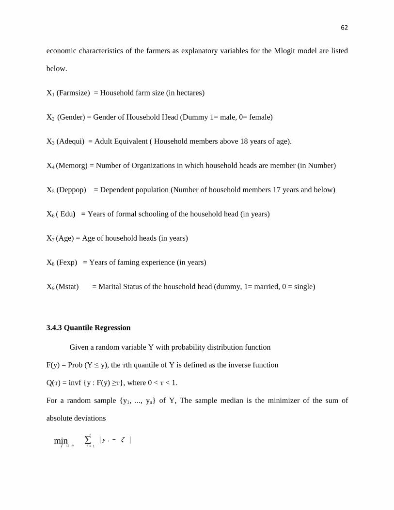
62
economic characteristics of the farmers as explanatory variables for the Mlogit model are listed
below.
X1 (Farmsize) = Household farm size (in hectares)
X2 (Gender) = Gender of Household Head (Dummy 1= male, 0= female)
X3 (Adequi) = Adult Equivalent ( Household members above 18 years of age).
X4 (Memorg) = Number of Organizations in which household heads are member (in Number)
X5 (Deppop) = Dependent population (Number of household members 17 years and below)
X6 ( Edu) = Years of formal schooling of the household head (in years)
X7 (Age) = Age of household heads (in years)
X8 (Fexp) = Years of faming experience (in years)
X9 (Mstat) = Marital Status of the household head (dummy, 1= married, 0 = single)
3.4.3 Quantile Regression
Given a random variable Y with probability distribution function
F(y) = Prob (Y ≤ y), the ᴛth quantile of Y is defined as the inverse function
Q(ᴛ) = invf {y : F(y) ≥ᴛ}, where 0 < ᴛ < 1.
For a random sample {y1, ..., yn} of Y, The sample median is the minimizer of the sum of
absolute deviations
∑=∈
−n
iR
iy1
min ζζ
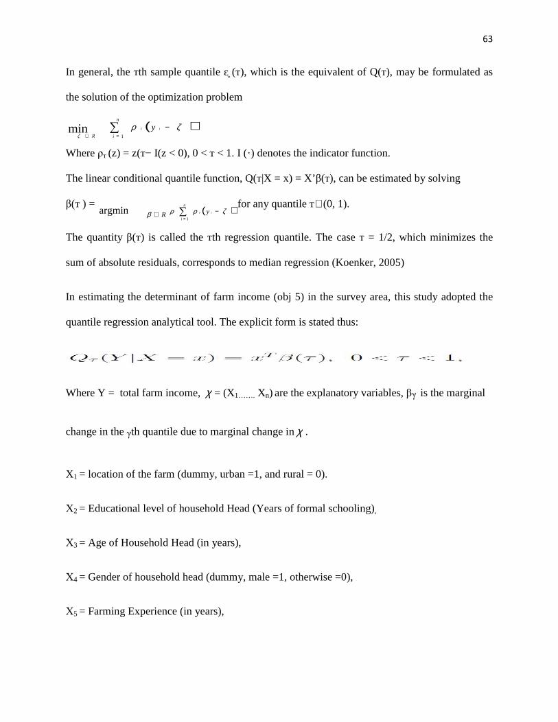
63
In general, the ᴛth sample quantile ᶓ (ᴛ), which is the equivalent of Q(ᴛ), may be formulated as
the solution of the optimization problem
( )∑=∈
−n
iR
iy1
min ζρ τ
ζ
Where ρᴛ (z) = z(ᴛ− I(z < 0), 0 < ᴛ < 1. I (·) denotes the indicator function.
The linear conditional quantile function, Q(ᴛ|X = x) = X’β(ᴛ), can be estimated by solving
β(ᴛ ) = ( )∑
=−∈
n
i
iyR1
argmin ζρρβ τ
for any quantile ᴛ∈(0, 1).
The quantity β(ᴛ) is called the ᴛth regression quantile. The case ᴛ = 1/2, which minimizes the
sum of absolute residuals, corresponds to median regression (Koenker, 2005)
In estimating the determinant of farm income (obj 5) in the survey area, this study adopted the
quantile regression analytical tool. The explicit form is stated thus:
Where Y = total farm income, χ = (X1……. Xn) are the explanatory variables, βᵧ is the marginal
change in the ᵧth quantile due to marginal change inχ .
X1 = location of the farm (dummy, urban =1, and rural = 0).
Х2 = Educational level of household Head (Years of formal schooling),
Х3 = Age of Household Head (in years),
Х4 = Gender of household head (dummy, male =1, otherwise =0),
Х5 = Farming Experience (in years),
64
Х6 = Marital Status (dummy, 1 if married, 0 = otherwise)
Х7 = household size (number of persons in the household)
Х8 = Farm size in ha (area owned by household),
Х9 = Access to formal or informal credit (dummy, if have access = 1, otherwise = 0),
X10 = Proximity to market (approximate distance to nearby market in km),
Х11 = Assets (value of productive asset owned by the household in naira),
Х12 = Non-farm income status (dummy, 1=if partake in off-farm income, 0 = otherwise)
In the analysis, total farm income was the dependent variable, while socioeconomic and
demographic characteristics (i.e. Farm location, educational level of household head, years of
farming experience, age, marital status, household size, land size, access formal credit, asset
value, gender, market proximity and Non-farm income) served as explanatory variables. The
quantile regression at 25th, 50th, and 75th quantiles was applied to examine how socio-
demographic factors affect the income distribution in urban farm households. In fact, a large
number of studies has explored the theory background and application of quantile regression, and
also made a clear comparison about Ordinary Least Squares regression (OLS) and quantile
regression. It is crucial to note that the Ordinary Least Squares regression estimates the
relationship between the set of explanatory variables and the conditional mean of the response
variable, while the quantile regression extends the regression model to conditional quantiles of a
response variable, such as the 10th, or 90th quantile. Just as the mean gives an incomplete
picture of a single distribution, the regression curve of the OLS also gives a corresponding
incomplete picture for a set of distributions, thus we could compute several different regression
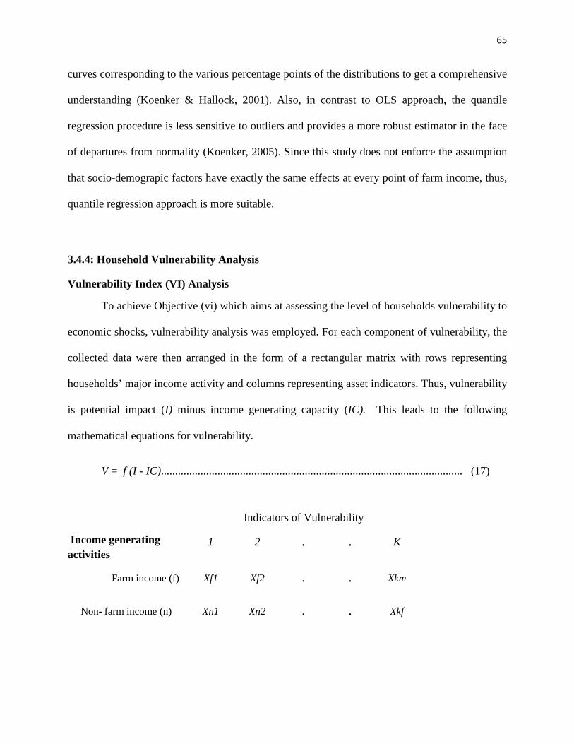
65
curves corresponding to the various percentage points of the distributions to get a comprehensive
understanding (Koenker & Hallock, 2001). Also, in contrast to OLS approach, the quantile
regression procedure is less sensitive to outliers and provides a more robust estimator in the face
of departures from normality (Koenker, 2005). Since this study does not enforce the assumption
that socio-demograpic factors have exactly the same effects at every point of farm income, thus,
quantile regression approach is more suitable.
3.4.4: Household Vulnerability Analysis
Vulnerability Index (VI) Analysis
To achieve Objective (vi) which aims at assessing the level of households vulnerability to
economic shocks, vulnerability analysis was employed. For each component of vulnerability, the
collected data were then arranged in the form of a rectangular matrix with rows representing
households’ major income activity and columns representing asset indicators. Thus, vulnerability
is potential impact (I) minus income generating capacity (IC). This leads to the following
mathematical equations for vulnerability.
V = f (I - IC)........................................................................................................... (17)
Income generating activities
Indicators of Vulnerability
1 2 . . K
Farm income (f) Xf1 Xf2 . . Xkm
Non- farm income (n) Xn1 Xn2 . . Xkf
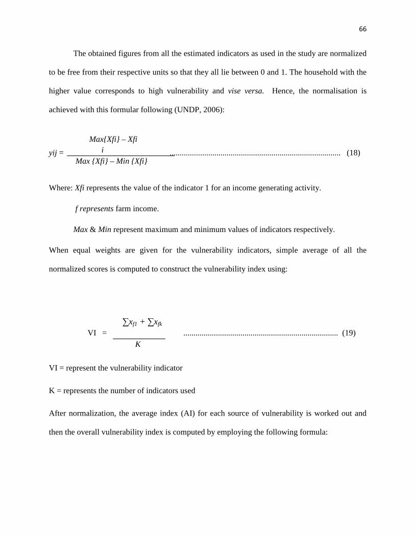
66
The obtained figures from all the estimated indicators as used in the study are normalized
to be free from their respective units so that they all lie between 0 and 1. The household with the
higher value corresponds to high vulnerability and vise versa. Hence, the normalisation is
achieved with this formular following (UNDP, 2006):
yij = .................................................................................... (18)
Where: Xfi represents the value of the indicator 1 for an income generating activity.
f represents farm income.
Max & Min represent maximum and minimum values of indicators respectively.
When equal weights are given for the vulnerability indicators, simple average of all the
normalized scores is computed to construct the vulnerability index using:
VI = ............................................................................ (19)
VI = represent the vulnerability indicator
K = represents the number of indicators used
After normalization, the average index (AI) for each source of vulnerability is worked out and
then the overall vulnerability index is computed by employing the following formula:
∑xf1 + ∑xfk
j j K
Max{Xfi} – Xfi i
Max {Xfi} – Min {Xfi}
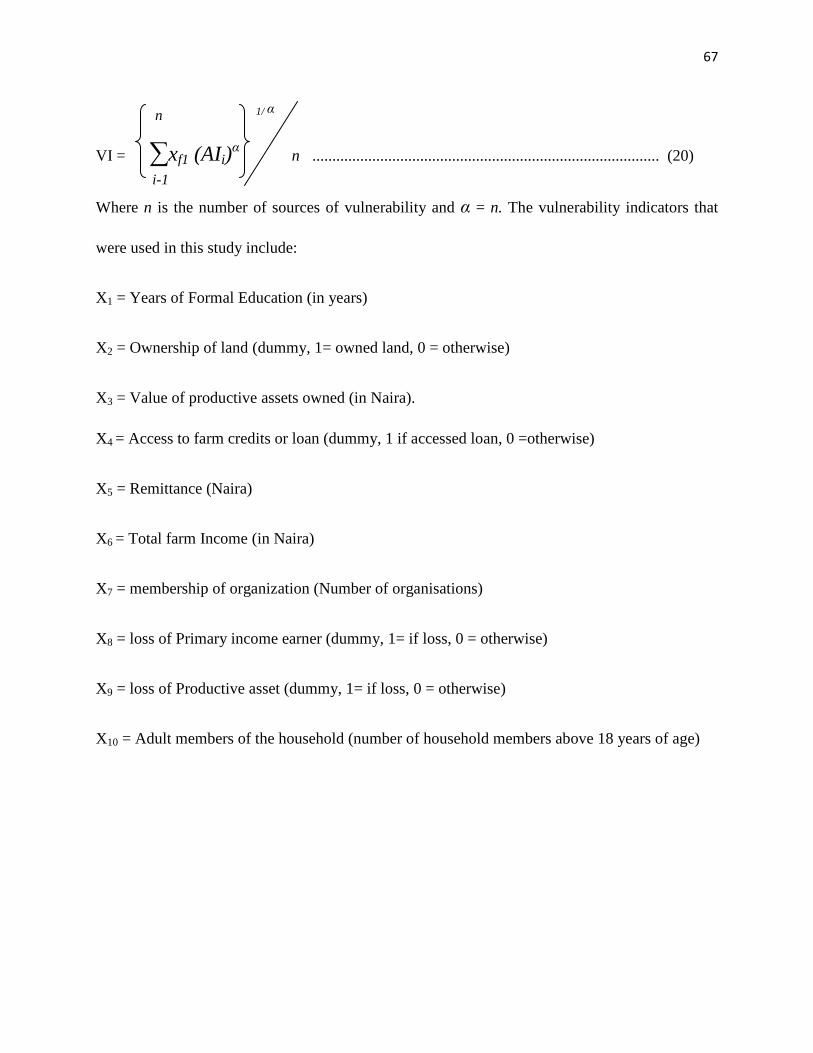
67
VI = ∑xf1 (AIi)α ....................................................................................... (20)
Where n is the number of sources of vulnerability and α = n. The vulnerability indicators that
were used in this study include:
X1 = Years of Formal Education (in years)
X2 = Ownership of land (dummy, 1= owned land, 0 = otherwise)
X3 = Value of productive assets owned (in Naira).
X4 = Access to farm credits or loan (dummy, 1 if accessed loan, 0 =otherwise)
X5 = Remittance (Naira)
X6 = Total farm Income (in Naira)
X7 = membership of organization (Number of organisations)
X8 = loss of Primary income earner (dummy, 1= if loss, 0 = otherwise)
X9 = loss of Productive asset (dummy, 1= if loss, 0 = otherwise)
X10 = Adult members of the household (number of household members above 18 years of age)
n
i-1
1/ α
n
68
CHAPTER FOUR
RESULTS AND DISCUSSION
4.1 Socio-economic characteristics of the respondents
In this chapter, the major socio-economic characteristics of households covered by the
survey are presented. These characteristics relate to age, level of education, household size,
farming experience, gender, marital status, major income generating activities, production
patterns, and household composition. The level of asset, the socio economic factors influencing
the choice of an income generating activity by the respondents, determinants of farm income
among the respondents and their level of vulnerability are also presented/ discussed.
4.1.1 Age of household heads
Rougoor, Ruud, Huine, & Renkema (1998) examined the significance of age on farm
output and observed that the influence of age on farm productivity is very diverse. Also, a study
by Adubi (1992) shows that age, in correlation with farming experience, has significant influence
on decision making process of farmers with respect to risk aversion, adoption of improved
technology and other production related decisions. Age has been found to determine how active
and productive the head of the household would be. It is also a strong determinant of the
probability of the household head getting involved in different income generating activities.
Table 4.1 shows the distribution of household heads by age ranges. The table shows that the age
distribution of household heads was fairly similar across the three surveyed States. But on the
average, approximately 69% of the household heads were between 31 and 50 years of age. The
mean age of the household heads was 44 years (with a standard deviation of 9.69). For the
sample as a whole, approximately 77% of the household heads were in the active and productive
age range. Only 23% of the respondents fell within the old age of lower productivity (more than
69
50 years). This shows that an average urban household head in the surveyed area was in his
middle years suggesting high economic productivity. This finding concurs with results of Etim &
Ukoha (2010) who observed that inability to generate income (or poverty incidence) is highest
(69%) and lowest (31%) when households are headed by persons within the age of 61-80 and 21-
40 years respectively. The predominance of active and productive heads of households among
the respondents has a direct bearing on increased availability of labour for production and
adoption of different income generating activities for survival/household poverty reduction and,
hence, improving households’ livelihoods in the study area.
4.1.2 Level of Education of Household heads.
The level of education could determine the level of opportunities available to improve
livelihood strategies, enhance food security and reduce the level of poverty. Educational level
also affects the level of exposure to new ideas and managerial capacity in production and the
perception of the household members on how to adopt and integrate innovations into the
household’s survival strategies. Household head’s educational level may determine the
household level of income as well as their decision to partake in different income generating
activities. According to Reardon, Berdegue, Barret & Stamoilis (2006), education is an important
part of human capital, which determines both participation in and income from non-farm
activities. The distribution of respondents according to level of education attained is shown in
Table 4.1. In all the three surveyed States, the pattern of distribution of the levels of formal
education was fairly similar. However, the highest literacy level was found in Akwa Ibom State,
with a mean educational level of 15.38 (16 denoting Higher National Diploma) and the lowest
literacy level was found in Cross River State (mean of 13.28). The mean educational level for the
whole sample was 14.39 years.
70
4.1.3 Household size of the respondents
The significance of household size in agriculture hinges on the possible availability of
labour for farm production, such that the total area cultivated to different crop enterprises and the
quantity of livestock reared could all be determined by the size of the farm household.
Household size could also boost household income especially when there are more income
earners in the household. The pattern of distribution of household sizes across the surveyed
States was similar. But, in relative terms, the mean household size was higher in Akwa Ibom
than Cross River and Delta States. The mean household size in the study area was approximately
5 persons (Table 4.1). Thus, a typical urban farming household is not large, which could indicate
a low supply of labour to the family enterprise.
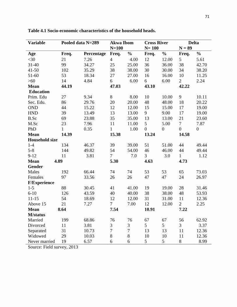
71
Table 4.1 Socio-economic characteristics of the household heads.
Variable Pooled data N=289 Akwa Ibom N=100
Cross River N= 100
Delta N = 89
Age Freq. Percentage Freq. % Freq. % Freq. % <30 21 7.26 4 4.00 12 12.00 5 5.61 31-40 99 34.27 25 25.00 36 36.00 38 42.70 41-50 102 35.29 38 38.00 30 30.00 34 38.20 51-60 53 18.34 27 27.00 16 16.00 10 11.25 >60 14 4.84 6 6.00 6 6.00 2 2.24 Mean 44.19 47.03 43.10 42.22 Education Prim. Edu 27 9.34 8 8.00 10 10.00 9 10.11 Sec. Edu. 86 29.76 20 20.00 48 48.00 18 20.22 OND 44 15.22 12 12.00 15 15.00 17 19.00 HND 39 13.49 13 13.00 9 9.00 17 19.00 B.Sc 69 23.88 35 35.00 13 13.00 21 23.60 M.Sc 23 7.96 11 11.00 5 5.00 7 7.87 PhD 1 0.35 1 1.00 0 0 0 0 Mean 14.39 15.38 13.24 14.58 Household size 1-4 134 46.37 39 39.00 51 51.00 44 49.44 5-8 144 49.82 54 54.00 46 46.00 44 49.44 9-12 11 3.81 7 7.0 3 3.0 1 1.12 Mean 4.89 5.30 4.63 4.73 Gender Males 192 66.44 74 74 53 53 65 73.03 Females 97 33.56 26 26 47 47 24 26.97 F/Experience 1-5 88 30.45 41 41.00 19 19.00 28 31.46 6-10 126 43.59 40 40.00 38 38.00 48 53.93 11-15 54 18.69 12 12.00 31 31.00 11 12.36 Above 15 21 7.27 7 7.00 12 12.00 2 2.25 Mean 8.64 7.54 10.91 7.22 M/status Married 199 68.86 76 76 67 67 56 62.92 Divorced 11 3.81 3 3 5 5 3 3.37 Separated 31 10.73 7 7 13 13 11 12.36 Widowed 29 10.03 8 8 10 10 11 12.36 Never married 19 6.57 6 6 5 5 8 8.99 Source: Field survey, 2013
72
4.1.4 Farming experience of household’s head
Farming experience is an important factor in determining both the productivity and the
production level. The influence of farming experience on productivity and production may be
positive or negative. Generally, it would appear that up to a certain number of years, farming
experience would have positive effect; after that, the effect may become negative. The negative
effect may be derived from aging or reluctance to change (Amaza, Tahirou, Patrick, & Amara,
2009). Table 4.1 shows that the farming experience of the respodents in the surveyed area varied
widely, with a minimum of only 2 years and a maximum of 58 years. The average farming
experience, however, did not vary widely across the States as the variation was between 7 years
in Delta State and Approximately 11 years in Cross River State. The mean farming experience in
the study area was approximately 9 years. This shows that the average urban farming household
head had a considerable experience in urban farming.
4.1.5 Gender of household’s head
Table 4.1 shows the distribution of the household heads according to gender. The table
shows that the percentage of male household heads (66.44%) was higher than female household
heads (33.56%). However, the female headed households were more (47%) in Cross River than
all the surveyed states (Akwa Ibom and Delta) which had an average of about 26%. The
predominance of female headed households in Cross River State could be attributed to their
tradition, which permits women inheritance to landed properties.
4.1.6 Marital Status of the household heads
The significance of marital status on agricultural production can be explained in terms of
supply of agricultural family labour. It is expected that family labour would be more available
73
where the household heads are married. Also, married households are expected to shoulder more
responsibilities which could require more income which in turns pushes them to partake on
different income generating activities. Adenegan, Adams & Nwauwa, (2013), observed that
being married determined the capability of the farm households to allocate their resources
efficiently on both farm and non-farm activities to boost the household income. Table 4.1 shows
that 76% in Akwa Ibom were married, while 67% and 62.92% were married in Cross River and
Delta States respectively. However, a cursory look at Table 4.1 shows that on the average, about
93.43% of the respondents were once married, while only 6.57% never got married.
4.1.7 Income generating activities of the household heads
In Sub-Saharan Africa, it is common for some poor urban dwellers to engage in different
income generating activities to reduce poverty and food insecurity. In this survey, income
generating activities were classified into seven different categories. These are presented in Table
4.2 and bar chart in figure 4.1, as major categories of income generating activities. The table
shows that non-agricultural wage income was the most important activity as 35.64% of the
households were involved. Crop production was the second most important activity (25% of the
respondents were involved). About 19.03 % of the surveyed household adopted income from
other sources as their major income source, 14.19 % of them adopted Livestock production as
the most important income generating activity. Agricultural wage employment income, income
from pension, rent, and shares, and remittance income were adopted by 2.77%, 1.73% and 1.04
% of the respondents respectively. This is an indication that agricultural wage income, income
from rent and remittances were not major sources of income in the surveyed area. The
dependence of urban families on farming (crops and animal production) may have a positive
effect on income generation of the household, depending on availability of land and allocation of
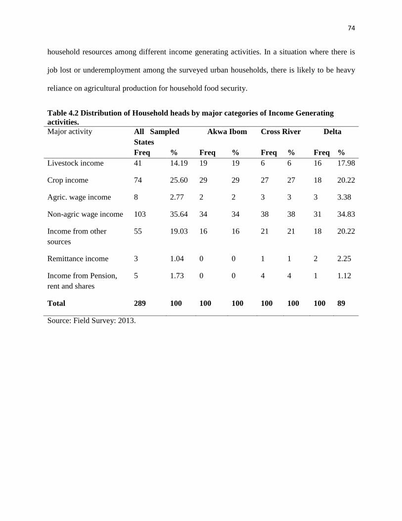
74
household resources among different income generating activities. In a situation where there is
job lost or underemployment among the surveyed urban households, there is likely to be heavy
reliance on agricultural production for household food security.
Table 4.2 Distribution of Household heads by major categories of Income Generating activities. Major activity All Sampled
States Akwa Ibom Cross River Delta
Freq % Freq % Freq % Freq % Livestock income 41 14.19 19 19 6 6 16 17.98
Crop income 74 25.60 29 29 27 27 18 20.22
Agric. wage income 8 2.77 2 2 3 3 3 3.38
Non-agric wage income 103 35.64 34 34 38 38 31 34.83
Income from other sources
55 19.03 16 16 21 21 18 20.22
Remittance income 3 1.04 0 0 1 1 2 2.25
Income from Pension, rent and shares
5 1.73 0 0 4 4 1 1.12
Total 289 100 100 100 100 100 100 89
Source: Field Survey: 2013.
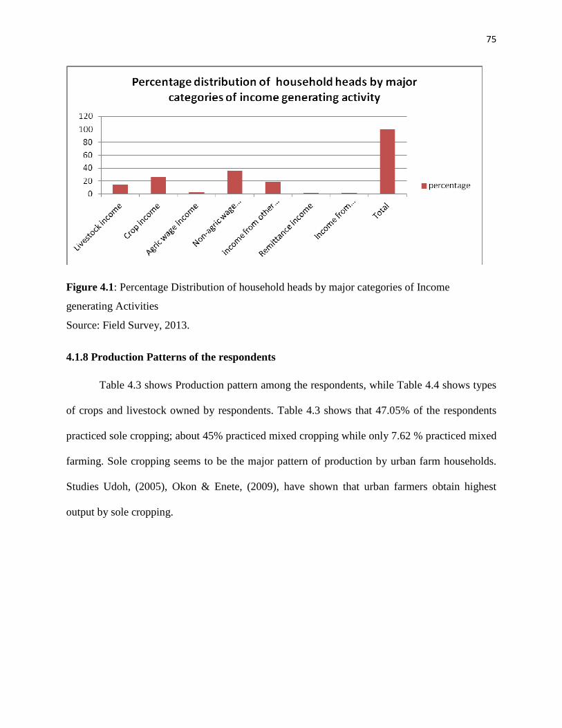
75
Figure 4.1: Percentage Distribution of household heads by major categories of Income
generating Activities
Source: Field Survey, 2013.
4.1.8 Production Patterns of the respondents
Table 4.3 shows Production pattern among the respondents, while Table 4.4 shows types
of crops and livestock owned by respondents. Table 4.3 shows that 47.05% of the respondents
practiced sole cropping; about 45% practiced mixed cropping while only 7.62 % practiced mixed
farming. Sole cropping seems to be the major pattern of production by urban farm households.
Studies Udoh, (2005), Okon & Enete, (2009), have shown that urban farmers obtain highest
output by sole cropping.
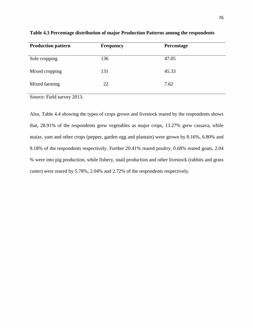
76
Table 4.3 Percentage distribution of major Production Patterns among the respondents
Production pattern Frequency Percentage
Sole cropping 136 47.05
Mixed cropping 131 45.33
Mixed farming 22 7.62
Source: Field survey 2013.
Also, Table 4.4 showing the types of crops grown and livestock reared by the respondents shows
that, 28.91% of the respondents grew vegetables as major crops, 13.27% grew cassava, while
maize, yam and other crops (pepper, garden egg and plantain) were grown by 8.16%, 6.80% and
9.18% of the respondents respectively. Further 20.41% reared poultry, 0.68% reared goats, 2.04
% were into pig production, while fishery, snail production and other livestock (rabbits and grass
cutter) were reared by 5.78%, 2.04% and 2.72% of the respondents respectively.
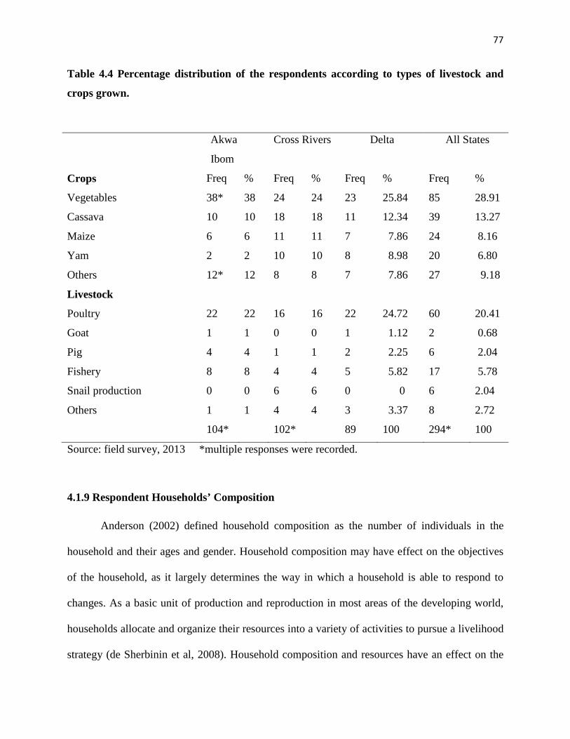
77
Table 4.4 Percentage distribution of the respondents according to types of livestock and
crops grown.
Source: field survey, 2013 *multiple responses were recorded.
4.1.9 Respondent Households’ Composition
Anderson (2002) defined household composition as the number of individuals in the
household and their ages and gender. Household composition may have effect on the objectives
of the household, as it largely determines the way in which a household is able to respond to
changes. As a basic unit of production and reproduction in most areas of the developing world,
households allocate and organize their resources into a variety of activities to pursue a livelihood
strategy (de Sherbinin et al, 2008). Household composition and resources have an effect on the
Akwa
Ibom
Cross Rivers Delta All States
Crops Freq % Freq % Freq % Freq %
Vegetables 38* 38 24 24 23 25.84 85 28.91
Cassava 10 10 18 18 11 12.34 39 13.27
Maize 6 6 11 11 7 7.86 24 8.16
Yam 2 2 10 10 8 8.98 20 6.80
Others 12* 12 8 8 7 7.86 27 9.18
Livestock
Poultry 22 22 16 16 22 24.72 60 20.41
Goat 1 1 0 0 1 1.12 2 0.68
Pig 4 4 1 1 2 2.25 6 2.04
Fishery 8 8 4 4 5 5.82 17 5.78
Snail production 0 0 6 6 0 0 6 2.04
Others 1 1 4 4 3 3.37 8 2.72
104* 102* 89 100 294* 100
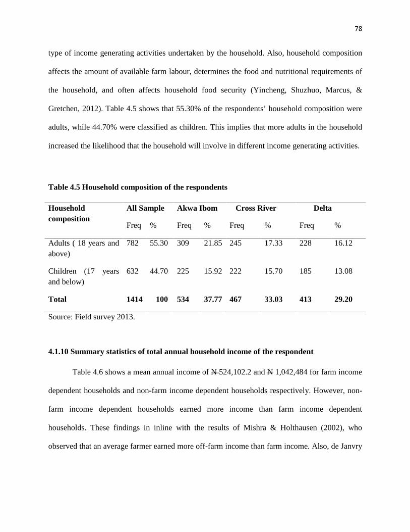
78
type of income generating activities undertaken by the household. Also, household composition
affects the amount of available farm labour, determines the food and nutritional requirements of
the household, and often affects household food security (Yincheng, Shuzhuo, Marcus, &
Gretchen, 2012). Table 4.5 shows that 55.30% of the respondents’ household composition were
adults, while 44.70% were classified as children. This implies that more adults in the household
increased the likelihood that the household will involve in different income generating activities.
Table 4.5 Household composition of the respondents
Household composition
All Sample Akwa Ibom Cross River Delta
Freq % Freq % Freq % Freq %
Adults ( 18 years and above)
782 55.30 309 21.85 245 17.33 228 16.12
Children (17 years and below)
632 44.70 225 15.92 222 15.70 185 13.08
Total 1414 100 534 37.77 467 33.03 413 29.20
Source: Field survey 2013.
4.1.10 Summary statistics of total annual household income of the respondent
Table 4.6 shows a mean annual income of N 524,102.2 and N 1,042,484 for farm income
dependent households and non-farm income dependent households respectively. However, non-
farm income dependent households earned more income than farm income dependent
households. These findings in inline with the results of Mishra & Holthausen (2002), who
observed that an average farmer earned more off-farm income than farm income. Also, de Janvry
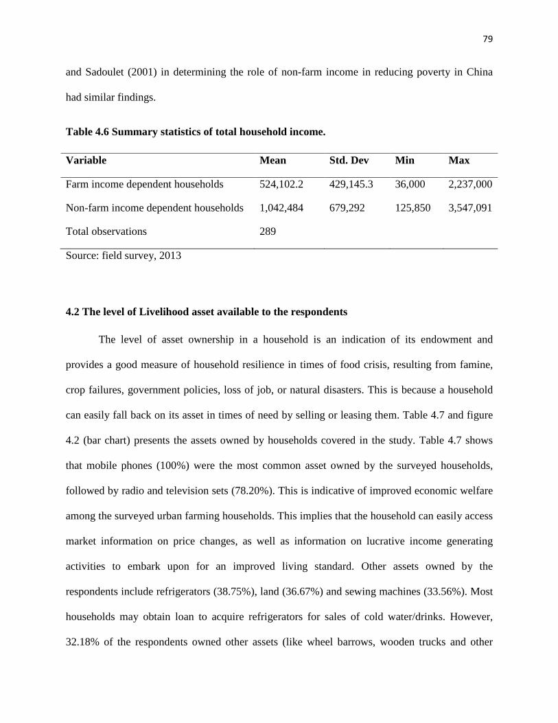
79
and Sadoulet (2001) in determining the role of non-farm income in reducing poverty in China
had similar findings.
Table 4.6 Summary statistics of total household income.
Variable Mean Std. Dev Min Max
Farm income dependent households 524,102.2 429,145.3 36,000 2,237,000
Non-farm income dependent households 1,042,484 679,292 125,850 3,547,091
Total observations 289
Source: field survey, 2013
4.2 The level of Livelihood asset available to the respondents
The level of asset ownership in a household is an indication of its endowment and
provides a good measure of household resilience in times of food crisis, resulting from famine,
crop failures, government policies, loss of job, or natural disasters. This is because a household
can easily fall back on its asset in times of need by selling or leasing them. Table 4.7 and figure
4.2 (bar chart) presents the assets owned by households covered in the study. Table 4.7 shows
that mobile phones (100%) were the most common asset owned by the surveyed households,
followed by radio and television sets (78.20%). This is indicative of improved economic welfare
among the surveyed urban farming households. This implies that the household can easily access
market information on price changes, as well as information on lucrative income generating
activities to embark upon for an improved living standard. Other assets owned by the
respondents include refrigerators (38.75%), land (36.67%) and sewing machines (33.56%). Most
households may obtain loan to acquire refrigerators for sales of cold water/drinks. However,
32.18% of the respondents owned other assets (like wheel barrows, wooden trucks and other
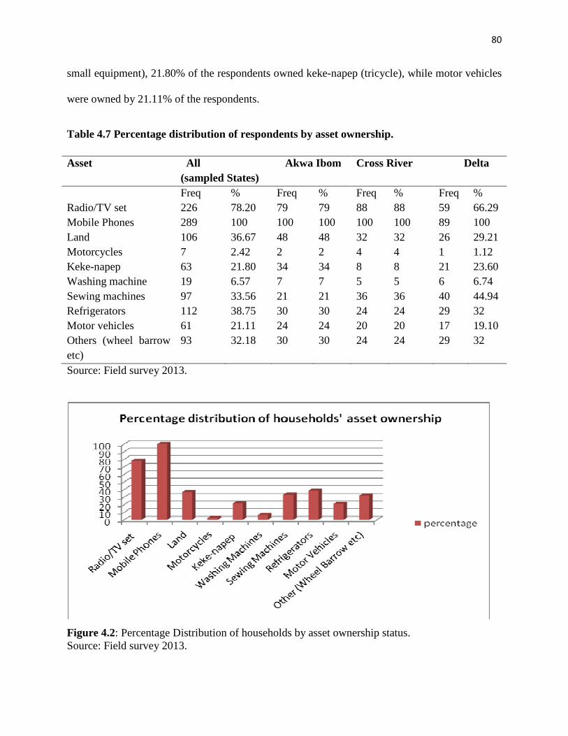
80
small equipment), 21.80% of the respondents owned keke-napep (tricycle), while motor vehicles
were owned by 21.11% of the respondents.
Table 4.7 Percentage distribution of respondents by asset ownership.
Asset All (sampled States)
Akwa Ibom Cross River Delta
Freq % Freq % Freq % Freq % Radio/TV set 226 78.20 79 79 88 88 59 66.29 Mobile Phones 289 100 100 100 100 100 89 100 Land 106 36.67 48 48 32 32 26 29.21 Motorcycles 7 2.42 2 2 4 4 1 1.12 Keke-napep 63 21.80 34 34 8 8 21 23.60 Washing machine 19 6.57 7 7 5 5 6 6.74 Sewing machines 97 33.56 21 21 36 36 40 44.94 Refrigerators 112 38.75 30 30 24 24 29 32 Motor vehicles 61 21.11 24 24 20 20 17 19.10 Others (wheel barrow etc)
93 32.18 30 30 24 24 29 32
Source: Field survey 2013.
Figure 4.2: Percentage Distribution of households by asset ownership status. Source: Field survey 2013.
81
4.3 Factors that determine households’ level of income from each category of income
generating activity.
The analysis of socio-economic factors that influence households’ level of income from
each categories of income (their major sources of income) is presented in Table 4.8. Four out of
the seven categories of income are presented. Three namely, agric. wage income, remittance
income and income from pension, rents and shares, are not presented because very few
households participated in them as their major income source.
Since all household obtained income, the total household income from each of the income
generating activity is estimated by OLS. The linear model was chosen as the best out of four
(linear, semi-log, double-log and exponential) functional forms in all income categories (see
appendix). The fit of the models are quite reasonable compared to models in the literature on
total household income. Table 4.8 presents the analysis of OLS result of the four categories of
income generating activities. The R2 are 0.61, 0.66, 0.29 and 0.55 for livestock income, crop
income, non-agricultural wage income and income from other sources respectively. This implies
that 61 %, 66 %, 29 % and 55 % of the variations in the livestock income, crop income, non-
agric wage income and income from other sources were explained by the independent variables
included in the model. The F–statistics of 5.40 (0.0002), 13.99 (0.0000), 4.32 (0.0001), and 6.14
(0.0000) for livestock income, crop income, non-agric wage and income from other sources
respectively was significant at 1 percent critical value, suggesting that all the models were of
good fit.
Education coefficient was found to be negative and not statistically significant in farm
income category (livestock income and crop income), although positive and significant in non-
agric wage income (p < 0.10) and, also in income from other sources (p < 0.01). Suggesting the
probability of involvement in non-farm activities among the surveyed household’s increases with
82
increase in educational level. Ferreira and Lanjouw (2001), observed that years of formal
education make the household heads more employable (for example, because they would be
more knowledgeable of employment opportunities and more adaptable in the range of task that
they can perform as a hired worker or self-employed). Also this finding is in consonance with the
results of Atamanov (2011), who observed that higher education significantly increased self-
employed income. Specifically, an individual educated beyond 14 years is found to be more
likely to work off-farm (Matshe & Young 2004).
Age could reflect the stage of life of the household head. The coefficient of age was
negative and not statistically significant in all the regressed income generating categories. This is
not surprising, perhaps because increasing the variable age (holding others constant) will
decrease the probability of generating income from any of the income generating categories. This
implies that older household heads may not be able to generate more income in all the regressed
income generating activities.
Gender may influence available opportunities for income generation. The coefficient of
gender although was not statistically significant, was positive in three (livestock income, non-
agric. wage income and income from other sources) out of the four regressed income generating
categories. However, the gender coefficient was negatively signed in crop income generating
category. This suggests that women were more likely to be involved in crop production
enterprise than their male counterpart. This agrees with the findings of Chant (2013) who
observed that women are more likely than men to be employed informally and tend to have less
well-paid and more insecure jobs.
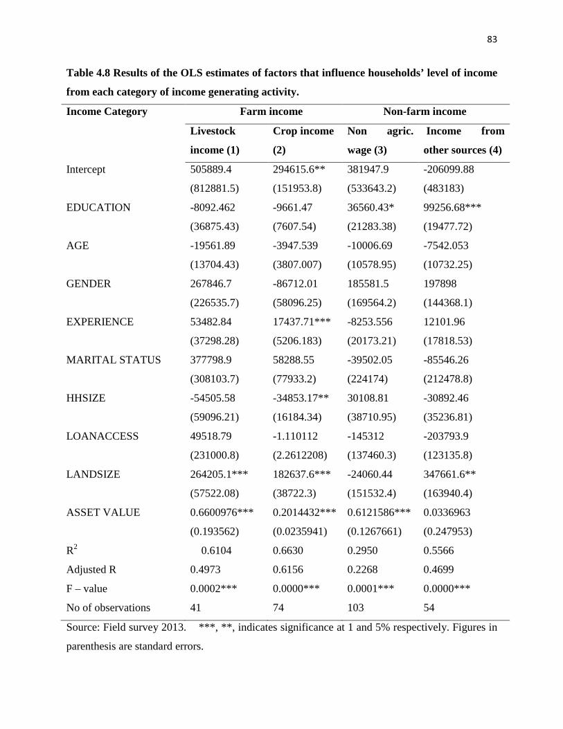
83
Table 4.8 Results of the OLS estimates of factors that influence households’ level of income
from each category of income generating activity.
Income Category Farm income Non-farm income
Livestock
income (1)
Crop income
(2)
Non agric.
wage (3)
Income from
other sources (4)
Intercept 505889.4
(812881.5)
294615.6**
(151953.8)
381947.9
(533643.2)
-206099.88
(483183)
EDUCATION
-8092.462
(36875.43)
-9661.47
(7607.54)
36560.43*
(21283.38)
99256.68***
(19477.72)
AGE -19561.89
(13704.43)
-3947.539
(3807.007)
-10006.69
(10578.95)
-7542.053
(10732.25)
GENDER
267846.7
(226535.7)
-86712.01
(58096.25)
185581.5
(169564.2)
197898
(144368.1)
EXPERIENCE
53482.84
(37298.28)
17437.71***
(5206.183)
-8253.556
(20173.21)
12101.96
(17818.53)
MARITAL STATUS 377798.9
(308103.7)
58288.55
(77933.2)
-39502.05
(224174)
-85546.26
(212478.8)
HHSIZE
-54505.58
(59096.21)
-34853.17**
(16184.34)
30108.81
(38710.95)
-30892.46
(35236.81)
LOANACCESS
49518.79
(231000.8)
-1.110112
(2.2612208)
-145312
(137460.3)
-203793.9
(123135.8)
LANDSIZE
264205.1***
(57522.08)
182637.6***
(38722.3)
-24060.44
(151532.4)
347661.6**
(163940.4)
ASSET VALUE
0.6600976***
(0.193562)
0.2014432***
(0.0235941)
0.6121586***
(0.1267661)
0.0336963
(0.247953)
R2 0.6104 0.6630 0.2950 0.5566
Adjusted R 0.4973 0.6156 0.2268 0.4699
F – value 0.0002*** 0.0000*** 0.0001*** 0.0000***
No of observations 41 74 103 54
Source: Field survey 2013. ***, **, indicates significance at 1 and 5% respectively. Figures in
parenthesis are standard errors.
84
The coefficient of farming experience was negative and not statistically significant in
non-agricultural wage income category. However, farming experience was positive and
statistically significant (p < 0.01) among the crop income dependent households, this implies that
increasing years of farming experience among crop farming household will have a significant
increase on their level of income, thereby improving their wellbeing. This result also confirmed
the findings by Adebayo (2012) who observed a positive relationship between farming
experience and household income.
Marital Status: Through marriage, household could gain access to family labour for
income generation. The coefficient of marital status was positive but not statistically significant
in all the four categories of income generating activity. Suggesting that being married
contributed positively to income generation. This could be because married household may have
more household members which could generate income from different activities.
The coefficient of household size was negative and statistically significant (p < 0.05) in
crop income generating category. The implication of this finding is that large household sizes are
more likely to have less income from crop production. A plausible explanation to this finding is
that large household sizes could consume farm produce which otherwise could have been sold
for income. This result further confirmed the findings by Okunmadewa, Yusuf & Omonona
(2007) who observed that a unit increase in household size is associated with 3.1 % increase in
poverty.
Coefficient of loan access was positive in livestock income model and negative in crop
income, non-agric wage income and income from other sources although it was not statistically
significant. This could mean that those households that are depending solely on livestock income
had access to loan (both formal and informal). A plausible explanation to this could be that most
85
livestock farmers in the surveyed area were members of social organizations which may have
given them access to agricultural credit. It could also be that lenders give more credit to livestock
farmers. This however, increased their income level thereby improving their wellbeing.
Land size has positive and statistically significant (p < 0.01) coefficient in both livestock
income and crop income and, also statistically significant (p < 0.05) in income from other
sources models. This is not surprising because land is an important factor in livestock and crop
production. This implies that a unit increase in land size will significantly increase household
income from both crop and livestock production. This result agrees with findings by Martey, Al-
Hassan, and kuwornu (2012) who observed that households with large farms have the potential
to increase their market surplus, hence increasing farm income. Furthermore, households
depending on income from other sources could use land as collateral in obtaining loans. This
could also boost their income level, thereby making them to escape from poverty.
The coefficient of asset value was positive and significant (p < 0.01) in livestock , crop
income and non-agric-wage income generating category. This is to be expected because assets
are very important in households’ income generation. The ability of a household to engage in a
more profitable income generating activity is dependents on their access to assets (Tacoli, 1998).
This could be because access to, control over and ownership of assets are critical components of
wellbeing (Cater & Barret, 2006). In addition, households’ assets can be used as a buffer against
harsh economic situations, thereby improving their welfare. Also, asset can act as collateral and
facilitate access to credit and financial services as well as increase social status. Bebbington
(1999) noted that “peoples asset are not merely means through which they make a living: they
also give meaning to the person’s world”.
86
4.4 Socio-economic factors influencing participation in income generating activities by
urban farm households in the study area.
In this analysis, the base category is “Non- Agricultural Wage Income (4)”. The results of
the multinomial logit model indicate that socio-economic factors (Farm size, gender, number of
adults in the household, number of organizations which the household head belongs to,
dependent population, educational status of household heads, age of household heads, farming
experience, and marital status) influenced the type of income generating activities (IGA)
practiced by the respondents.
The estimated coefficient of the MNL model along with the levels of significance, are
presented in Table 4.9. The results in Table 4.9 shows that the likelihood ratio (χ 2) is
statistically significant at the one percent level meaning that the variables considered jointly
exert a very significant influence on the choice of income generating activities. In terms of
consistency with a priori expectations on the relationship between the dependent and the
explanatory variables, the model appears to have performed well. However, the parameter
estimates of the MNL model provide only the direction of the effect of the independent variables
on the dependent (response) variable: estimates do not represent actual magnitude of change or
probabilities. Thus, the marginal effects from the MNL, which measure the expected change in
probability of a particular choice being made with respect to a unit change in an independent
variable, are reported and discussed. In all cases the estimated coefficients were compared with
the base category (Non- Agric Wage-Income). Table 4.10 presents the marginal effects along
with the levels of statistical significance.
Land Size is closely linked to agricultural production, including crop and livestock
production. Bigger land sizes increase the probability that the urban farm household will be
involved in Livestock income, Crop income and Agric-wage income. As can be observed in
87
Table 4.9 land size significantly increased the probability that an urban farm household will
choose livestock income (p < 0.01), crop income (p < 0.01) and agricultural wage income (p<
0.01) as their major income generating activities as opposed to non-agric wage income. Also, the
result of the marginal effect (table 4.10) indicates that an additional hectare of land ceteris
paribus will result in a 12.6%, 14.51% and 1.2% increase in the probability of household
participating in Livestock income, Crop income and Agric-wage income respectively as their
major income generating activities. Moreover, the coefficient of land size was positively and
statistically significant in all categories of farm income, suggesting a positive relationship
between land size and farm income. The relationship is not surprising, because livestock
production, crop production and agric. wage income require land for their operations. Adenagan,
Adam and Nwauwa (2013) also found a positive relationship between land size and farm
income.
Gender of Household Heads: The result in Table 4.10 indicates that female headed
households are 35.99% more likely to choose crop income and 0.5% more likely to choose
remittance income as their major income generating activity, as opposed to Non- agricultural
wage income. This could be attributed to central and cultural role of women in household food
delivery. The marginal effect (table 4.10), also suggests that their male counterparts are 22.40%
more likely to choose Non- agricultural wage income as their major income generating activity.
This could be because, as compared to Non- agric wage income, crop income and remittance
income may not require educational qualification which most female headed households may not
have. Non- agric. wage income may require a certain level of education before one can be
gainfully employed.
88
Adult Household Members (Household members aged 18 years and above): Having more
adult members of the household is positively related to the likelihood that urban farming
household would partake in livestock or crop production as their major income generating
activity. This could be because of labour intensive nature of livestock and crop production in the
area, although the coefficients of adult household members were not statistically significant. The
implication of this result is that increasing adult members could increase household participation
in labour intensive IGA.
Membership of Organization (number of social organizations the household head belongs
to): The result in Table 4.9 shows that number of organizations the household heads belong to
lead to increased participation in livestock production, but has no statistically significant
influence on other categories of activities. The marginal effects (table 4.10) shows that being
membership of more than one organization increases the likelihood of urban farm household
choosing livestock production as their major income activity by 8.13 percent. The reason for this
might be that poultry production, the most common livestock activity, is produced by almost one
quarter of the surveyed households. The increasing cost of feed makes management of the
livestock a little difficult. Poultry farmers often get to know the best management practice by the
experiences of other farmers. Moreover, other farmers are often the most trusted and only source
of information on how they could manage their stock. Meetings of social organizations are a
good opportunity to meet other poultry farmers and discuss such issues.
Dependents Population (household members aged 17 and below; and above 65 years): As
expected, having more dependent members in a household reduces the probability that the
household will partake in livestock production, agricultural wage income, income from other
source, and income from pension, rents and shares (table 4.9). Conversely, dependent population
89
increases the likelihood that the surveyed urban farm household will choose crop income and
remittance income as their major IGA, as opposed to non- agricultural wage income. This is to
be expected because, remittance income is mostly sent to dependent members (unemployed and
students) of a household to cater for their welfare and school fees. In addition, the non-technical
aspect of crop production (fruit harvesting, and cassava planting) could be done by dependent
population. However, the coefficients are not statistically significant across all categories of
income generating activity.
Years of Education: Table 4.9 shows that holding other variables constant, a one year
increase in the years of education of household head’s decreases the probability of the household
choosing livestock income, crop income and agricultural wage income by 0.06%, 7.76% and
0.04% respectively as opposed to non- agric wage income. In other words, a one year increase in
education of household head decreases the probability of participation in livestock production,
crop production and agric. wage income. The implication of this finding is that more educated
household heads could be gainfully employed in government organizations, and as such, may not
participate in farm income activities. This finding agrees with the results of Reardon, Berdegue
& Escorbar (2001) who asserted that, more educated people avoid farm wage employment and
are mostly engaged in non-farm wage employment. Also, de Janvry, Sadoulet and Zhu (2005),
found a positive relationship between education and participation in non-agricultural
employments. In addition, Taylor and Yunez-Naude (2000) observed that the human capital of
household as measured by schooling is expected to generally be linked to non-agricultural
activities, since this is where the returns to education are more likely to be highest.
Age of Household Heads: Table 4.10 shows that a one unit increase in age of household
heads statistically increases the likelihood of the urban farm household choosing remittance and
90
income from pension, rents and shares, while a one unit increase in age ceteris paribus,
decreases the likelihood of the respondent choosing income from other sources (by 1.2%),
livestock income, crop income, or agric. wage income as their major income generating
activities. The implication of this result is that livestock production, crop production and agric
wage employment could be labour intensive, and as such; the aged household heads may not be
energetic enough to carry out their activities.
Years of farming Experience: Table 4.9 shows that years of farming experience has a
positive and significant effect on household’s choice of income generating activities. For
instance (table 4.10), a unit increase in years of experience of household heads results in a
0.44%, 1.56%, 0.19% and 0.85% increase in the probability of participating in livestock income,
crop income, agric. wage income and income from other sources respectively as opposed to
non-agricultural wage income.
The coefficient of marital status was not statistically significant (table 4.9). The table
shows that marital status has a negative relationship with farm income categories (livestock
income, crop income and agric. wage income), but a positive relationship with non-farm income
categories (non-agricultural wage income, income from other sources, remittance and income
from pension, rents and shares).
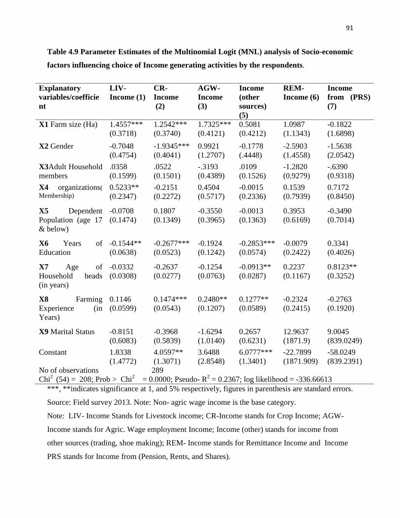
91
Table 4.9 Parameter Estimates of the Multinomial Logit (MNL) analysis of Socio-economic
factors influencing choice of Income generating activities by the respondents.
Explanatory variables/coefficient
LIV-Income (1)
CR- Income (2)
AGW-Income (3)
Income (other sources) (5)
REM-Income (6)
Income from (PRS) (7)
X1 Farm size (Ha) 1.4557*** (0.3718)
1.2542*** (0.3740)
1.7325*** (0.4121)
0.5081 (0.4212)
1.0987 (1.1343)
-0.1822 (1.6898)
X2 Gender -0.7048 (0.4754)
-1.9345*** (0.4041)
0.9921 (1.2707)
-0.1778 (.4448)
-2.5903 (1.4558)
-1.5638 (2.0542)
X3Adult Household members
.0358 (0.1599)
.0522 (0.1501)
-.3193 (0.4389)
.0109 (0.1526)
-1.2820 (0.9279)
-.6390 (0.9318)
X4 organizations( Membership)
0.5233** (0.2347)
-0.2151 (0.2272)
0.4504 (0.5717)
-0.0015 (0.2336)
0.1539 (0.7939)
0.7172 (0.8450)
X5 Dependent Population (age 17 & below)
-0.0708 (0.1474)
0.1807 (0.1349)
-0.3550 (0.3965)
-0.0013 (0.1363)
0.3953 (0.6169)
-0.3490 (0.7014)
X6 Years of Education
-0.1544** (0.0638)
-0.2677*** (0.0523)
-0.1924 (0.1242)
-0.2853*** (0.0574)
-0.0079 (0.2422)
0.3341 (0.4026)
X7 Age of Household heads (in years)
-0.0332 (0.0308)
-0.2637 (0.0277)
-0.1254 (0.0763)
-0.0913** (0.0287)
0.2237 (0.1167)
0.8123** (0.3252)
X8 Farming Experience (in Years)
0.1146 (0.0599)
0.1474*** (0.0543)
0.2480** (0.1207)
0.1277** (0.0589)
-0.2324 (0.2415)
-0.2763 (0.1920)
X9 Marital Status -0.8151 (0.6083)
-0.3968 (0.5839)
-1.6294 (1.0140)
0.2657 (0.6231)
12.9637 (1871.9)
9.0045 (839.0249)
Constant 1.8338 (1.4772)
4.0597** (1.3071)
3.6488 (2.8548)
6.0777*** (1.3401)
-22.7899 (1871.909)
-58.0249 (839.2391)
No of observations 289 Chi2 (54) = 208; Prob > Chi2 = 0.0000; Pseudo- R2 = 0.2367; log likelihood = -336.66613
***, **indicates significance at 1, and 5% respectively, figures in parenthesis are standard errors.
Source: Field survey 2013. Note: Non- agric wage income is the base category.
Note: LIV- Income Stands for Livestock income; CR-Income stands for Crop Income; AGW-
Income stands for Agric. Wage employment Income; Income (other) stands for income from
other sources (trading, shoe making); REM- Income stands for Remittance Income and Income
PRS stands for Income from (Pension, Rents, and Shares).
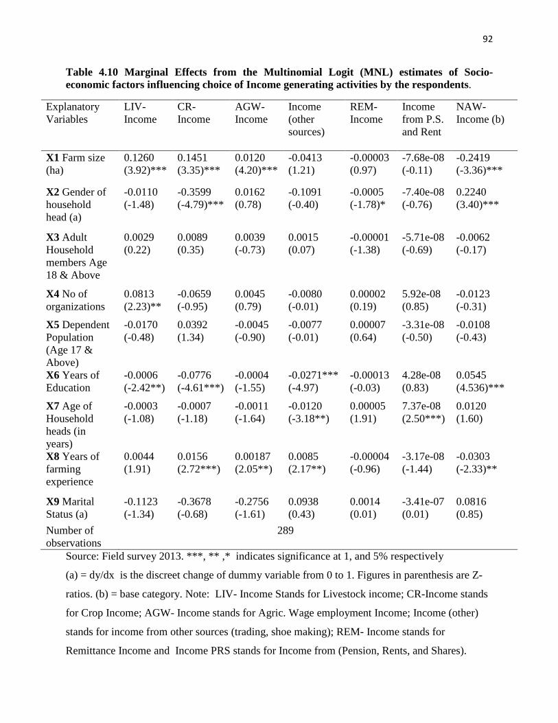
92
Table 4.10 Marginal Effects from the Multinomial Logit (MNL) estimates of Socio-economic factors influencing choice of Income generating activities by the respondents.
Explanatory Variables
LIV-Income
CR-Income
AGW-Income
Income (other sources)
REM-Income
Income from P.S. and Rent
NAW-Income (b)
X1 Farm size (ha)
0.1260 (3.92)***
0.1451 (3.35)***
0.0120 (4.20)***
-0.0413 (1.21)
-0.00003 (0.97)
-7.68e-08 (-0.11)
-0.2419 (-3.36)***
X2 Gender of household head (a)
-0.0110 (-1.48)
-0.3599 (-4.79)***
0.0162 (0.78)
-0.1091 (-0.40)
-0.0005 (-1.78)*
-7.40e-08 (-0.76)
0.2240 (3.40)***
X3 Adult Household members Age 18 & Above
0.0029 (0.22)
0.0089 (0.35)
0.0039 (-0.73)
0.0015 (0.07)
-0.00001 (-1.38)
-5.71e-08 (-0.69)
-0.0062 (-0.17)
X4 No of organizations
0.0813 (2.23)**
-0.0659 (-0.95)
0.0045 (0.79)
-0.0080 (-0.01)
0.00002 (0.19)
5.92e-08 (0.85)
-0.0123 (-0.31)
X5 Dependent Population (Age 17 & Above)
-0.0170 (-0.48)
0.0392 (1.34)
-0.0045 (-0.90)
-0.0077 (-0.01)
0.00007 (0.64)
-3.31e-08 (-0.50)
-0.0108 (-0.43)
X6 Years of Education
-0.0006 (-2.42**)
-0.0776 (-4.61***)
-0.0004 (-1.55)
-0.0271*** (-4.97)
-0.00013 (-0.03)
4.28e-08 (0.83)
0.0545 (4.536)***
X7 Age of Household heads (in years)
-0.0003 (-1.08)
-0.0007 (-1.18)
-0.0011 (-1.64)
-0.0120 (-3.18**)
0.00005 (1.91)
7.37e-08 (2.50***)
0.0120 (1.60)
X8 Years of farming experience
0.0044 (1.91)
0.0156 (2.72***)
0.00187 (2.05**)
0.0085 (2.17**)
-0.00004 (-0.96)
-3.17e-08 (-1.44)
-0.0303 (-2.33)**
X9 Marital Status (a)
-0.1123 (-1.34)
-0.3678 (-0.68)
-0.2756 (-1.61)
0.0938 (0.43)
0.0014 (0.01)
-3.41e-07 (0.01)
0.0816 (0.85)
Number of observations
289
Source: Field survey 2013. ***, ** ,* indicates significance at 1, and 5% respectively
(a) = dy/dx is the discreet change of dummy variable from 0 to 1. Figures in parenthesis are Z-
ratios. (b) = base category. Note: LIV- Income Stands for Livestock income; CR-Income stands
for Crop Income; AGW- Income stands for Agric. Wage employment Income; Income (other)
stands for income from other sources (trading, shoe making); REM- Income stands for
Remittance Income and Income PRS stands for Income from (Pension, Rents, and Shares).
93
4.5 Quantile regression estimates of the determinants of farm income among urban farm
households in the study area.
Socio-demographic factors that determine the level of farm income in the surveyed area
were analyzed using quantile regression. Table 4.11 displays the estimation results of the
quantile regression at 25th, 50th and 75th quantiles, as well the ordinary least square results (OLS).
The first three columns show the quantile regression results and as a comparison, the last column
is the OLS results.
Farm location coefficient was positive and not statistically significant at the 25th and 50th
income quantiles (i.e two lowest quantiles), but was negative and statistically significant (p <
0.01) at 75th income quantiles, and also at mean level (table 4.11). This finding stresses that,
household whose farm land are located in the urban centers made less income than households
whose farm land are located in rural areas. This finding has implication on economy of scale,
because urban farmers are land constrained, they may not be able to expand their farm land to
produce more income. However, urban agriculture is not a recognized land use activity in
Nigeria. As such there is no policy guide on urban farming that could warrant farmland
expansion.
Table 4.11 shows that educational level was found to be a significant factor. At the 25th
and 50th quantiles, the coefficient of education was positive but not statistically significant.
Interestingly, at 75th quantile, educational attainment was negative and statistically significant (P
< 0.01). The implication of this is that higher educational attainment reduces participation in
farm income (Reardon, Berdegue, & Escobar, 2001). Perhaps, because highly educated
household heads will work in wage employment. Also as farm income increases, there is every
indication that highly educated household heads will tend to divert income from farm to other
non-farm activity.
94
The coefficient of age was positively correlated with farm income across all quantiles,
and at mean level (table 4.11). At 50th and 75th quantiles, the coefficient of age was statistically
significant (p < 0.01). This findings stresses that farm income increases with age. Perhaps,
because as the household head grows older, he may gain new skills which could improve farm
profit, thereby increasing income, but again this response may be tempered when the farmer is
too old (from seventy years and above). Also, in a traditional African society, older household
heads have better access to land resource which is an important factor of production unlike the
younger household heads that mainly rely on inherited land (Taruvinga & Mushunje, 2010).
This finding also supports the role of age in resource ownership (Mukundi, Mathenge & Ngigi,
2013), in determining household decision to join Community forest.
Gender is an important indicator of household decision making whereby in a traditional
African set-up, key decisions in the household are made by men. Gender also depicts preferences
(choice of an income generating activity) of male and female household heads. The coefficient of
gender was positively correlated with farm income across all quantiles, and at mean level (table
4.11). At 75th quantile, the coefficient of gender was positive and statistically significant. The
implication of this finding is that men earn more income from all sources than women. This
result confirmed the findings of Okorji (1988), who observed that household income were
erroneously skewed in favour of men although women may earn more income. This could be
attributed to the importance of gender in defining specialization of labour supply within a
household. This finding also agrees with observation of Musyoki, Mugwe, Mutundu & Muchiri
(2013).
Farming experience coefficient was negatively correlated with farm income (table 4.11).
This is counter intuitive because one could expect that years of experience in farming could
95
increase farm income, but this is not the case here. This could be because experienced household
head may not have gotten enough farm land to display their wealth of experience which could
improve farm income. Also, in the life cycle of a farmer, point of decreasing marginal labour
productivity is anticipated whereby further increase in farming experience is expected to be
negatively associated with farm income (Amaza, Tahirou, Patrick, & Amara, 2009).
Marital status had a negative effect on farm income (table 4.11). Also, at 50th and 75th
quantiles, the coefficient of marital status was negative and statistically significant (p < 0.01).
This finding is consistent with the observation that married household are inclined to have less
income than their single counterpart (Reardon, Berdegue, & Escobar, 2001). This could be
because married household could have more household members that consume farm produce,
which otherwise could have been sold for money.
Household size had a negative and significant influence on farm income (table 4.11). At
lower income quantiles (25th and 50th quantiles) the coefficient of household size was negative
and not statistically significant, but negative and statistically significant (p < 0.01) at 75th income
quantile. This means that bigger household sizes reduce farm income. The same explanation in
marital status could also apply here. This is true because a typical urban farming household could
have relatives (who could be unemployed) staying with them while searching for white collar
jobs. As farm income increases, this could attract more members of the extended family into
their household thereby increasing the household size.
Land is an asset that is very useful across a range of activities and has a direct value in
agricultural production, although it can be used for different agricultural activities. It may have
an indirect value in other economic activities, as it could be used as collateral for credit. As
expected, the coefficient of land size had a positive and significant relationship with farm income
96
(table 4.11). It is expected that as land size increases, this could discourage participation in non-
farm activities, since increase in land size would help to lower cost of production, thereby
increasing farm income. Several studies, Yunez-Naude & Taylor (2001); Winters, Davis &
Corral, (2002); Adams, (2002) and de Janvry, Sadoulet & Zhu, (2005), found a positive
relationship between land size and farm income.
Loan access was negatively correlated with farm income across all income quantiles, and
at mean level (table 4.11). At 50th and 75th quantiles loan access was negative and statistically
significant (p < 0.01). The implication of this finding is that farm household that had access to
loan in the last two years, could diversify their farm income into non-farm activities when their
farm income increases. It could also mean that households who had access to loan could divert
the loan to other income generating activities.
Market proximity has economic implication on the household farm and market activities
(Owuor, 2009). A positive significant coefficient of the household distance to the market is an
indication of the relative effect of transaction cost to the household’s socio-economic activities.
Market proximity affects farm income in terms of travel time and costs. The analysis shows that,
distance to the market had a positive effect on farm income at the lower income quantiles (25th
and 50th), and at mean level. At 75th income quantile, market proximity had a negative and
statistically significant (p < 0.01) relationship with farm income (table 4.11). A plausible
explanation for this finding could be attributed to farm location (urban or rural). Interestingly,
household whose farm land are located in rural areas made more income than their counterpart
whose farm land are located in urban centers (explanation for location could also apply here).
Also, these same groups of household (who are at higher income quantile) are far from
97
agricultural market. This could be the reason why market proximity was negative at the 75th
income quantile.
Table 4.11 shows that asset value was positive and statistically significant (p<0.01) both
at the 75th income quantile and at mean level. This result stresses the important of assets in
income generating activities. Lack of assets is seen as both symptom and cause of poverty (de
Janvry & Sadoulet, 2000). In addition, assets support consumption by contribution to overall
production and income and allowing exchange and/or consumption in periods when there is no
income.
Non-farm Income (off- farm status) coefficient was negative and not significant at the
lower income quantiles (table 4.11). However, it had a positive and statistically significant (P <
0.01) coefficient at the 75th income quantile, and also statistically significant (p < 0.05) at mean.
This finding stresses the important of off-farm income on farm income. The implication of this
finding is that as off-farm income increases, there is every indication that the farm household
will invest the off-farm income in farm technology to boost production volume, which thereby
increases farm income. Marthy, Al-Hassan & Kuwornu (2012) also had similar findings. Also,
Matshe & Young (2004) observed that non-farm income has positive spin-offs in agricultural
performance by providing cash for productivity, enhancing inputs, thus easing credit constraints.
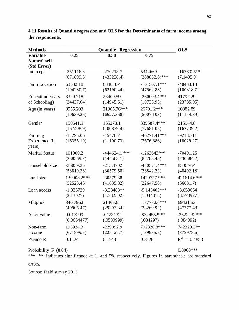
98
4.11 Results of Quantile regression and OLS for the Determinants of farm income among the respondents. Methods Quantile Regression OLS Variable Name/Coeff (Std Error)
0.25 0.50 0.75
Intercept -351116.3 (671899.5)
-270218.7 (433228.4)
5344669 (288832.6)***
-1678326** (7.1495.9)
Farm Location 63532.18 (104280.7)
6348.374 (62190.44)
-161567.1*** (47562.83)
-48433.13 (100318.7)
Education (years of Schooling)
3320.718 (24437.04)
23400.59 (14945.61)
-260003.4*** (10735.95)
41797.29 (23785.05)
Age (in years) 8555.203 (10639.26)
21305.76*** (6627.368)
26701.2*** (5007.103)
10382.89 (11144.39)
Gender 150641.9 (167408.9)
165273.1 (100839.4)
339587.4*** (77681.05)
215944.8 (162739.2)
Farming Experience (in years)
-14295.06 (16355.19)
-15476.7 (11190.73)
-46271.41*** (7676.886)
-9218.711 (18029.27)
Marital Status 101000.2 (238569.7)
-444624.1 *** (144563.1)
-1263643*** (84783.48)
-70401.25 (230584.2)
Household size -35039.35 (53810.33)
-213.8702 (30579.58)
-440571.4*** (23842.22)
8306.954 (48492.18)
Land size 139908.2*** (52523.46)
-30579.38 (41635.82)
1429727 *** (22647.58)
421614.6*** (66081.7)
Loan access -1.926729 (2.13027)
-3.23483** (1.382502)
-5.145402*** (1.044318)
-3.659664 (8.770927)
Mktprox 340.7962 (40906.47)
21465.6 (29293.34)
-187782.6*** (23260.92)
69421.53 (47777.48)
Asset value 0.017299 (0.0664477)
.0123132 (.0530999)
.8344552*** (.034297)
.2622232*** (.084092)
Non-farm income
195924.3 (671899.5)
-229092.9 (225127.7)
702820.8*** (189985.5)
742320.3** (378978.6)
Pseudo R 0.1524 0.1543 0.3828 R2 = 0.4853 Probability F (8.64) 0.0000*** ***, **, indicates significance at 1, and 5% respectively. Figures in parenthesis are standard
errors.
Source: Field survey 2013
99
4.6 Urban farm households’ vulnerability to economic shocks in the study area.
Households face different kinds and magnitude of risk that may lead to a wide variation
in their income from year to year including loss of productive assets (Alayande & Alayande,
2004). When there are not enough assets to reduce shocks or risk to livelihood, household
sometimes may experience losses including reduction in quality and quantity of nutritious food
intake; or sometimes school-aged children can temporally or permanently stop schooling
(Osawe, 2013), this could reduce household human capital base, thereby making them vulnerable
to economic shocks.
The estimation of household vulnerability to economic shocks was done using asset
capacity approach. Table 4.12 and figure 4.3 shows vulnerability analysis of the respondents.
The vulnerability indicators assessed in this study include: years of formal schooling (education),
land ownership status of the farmer, asset value, access to loan, access to remittance to support
farming, total farm income, membership of social organizations, loss of primary income earners
in the last five years, loss of productive asset in the last five years, and number of adult members
of household. It is assumed that most of these factors either reduces or increases respondents’
vulnerability to economic shocks. As presented in Table 4.12, the actual values of the asset base
indicators are in different units and scales. To obtain the vulnerability indices on each of the
indicators, the methodology used by United Nations Development Programme (UNDP) (2006)
for assessing Human Development Index was followed to normalize and standardize the values
to lie between 0 and 1. A value less than 0.5 implies that the household is not vulnerable to
economic shocks, while value greater than 0.5 indicates that the household is vulnerabile to
economic shocks. The most preferred and natural candidate for the vulnerability threshold is 0.5.
This midway dividing point has an attractive feature, it makes intuitive sense to say a household
is ‘vulnerable’ if it faces a 50 % or higher probability of falling into poverty in the near future.
100
The underlying logic is that “the observed poverty rate represents the mean vulnerability level in
the population, anyone whose vulnerability level lies above this threshold faces the risk of
poverty that is greater than the average risk in the population and hence can be legitimately be
included among the vulnerable” (Chaudhuri, 2003). In practice, therefore most of the empirical
studies adopted the vulnerability threshold of 0.5.
Using Education of the household heads as an indicator, farm income dependent
households in the surveyed area had vulnerability index of 0.69 while non-farm income
dependent households had vulnerability index of 0.20. The implication of this finding is that
farm income dependent households are 69 % vulnerable to economic shocks, while their non-
farm income dependent counterparts are not vulnerable. It could also mean that farm income
dependent household had low educational qualifications which could deny them opportunities to
be employed in more remunerative jobs, which otherwise could assist them to cope with
economic shocks. It is worthy to note that poverty and vulnerability diminishes as we move up
the education ladder (Osawe, 2013). Education can affect people’s standard of living through a
number of channels: it helps skill formation resulting in higher marginal productivity of labour
that eventually enables people to engage in more remunerative jobs. Highly educated people may
have better coping abilities against future odds. Indeed, educated people may adapt more easily
to changing circumstances, therefore showing greater ex-post coping capacity (Christiansen &
Subbarao, 2005).
Considering land ownership status, farm income dependent households had vulnerability
index of 0.86, suggesting 86 % vulnerability, while non-farm income dependent households were
not vulnerable (0.31). This implies that non-farm income dependent households’ had more
access to land than their counterparts. This is not unconnected to the high educational level of
101
non-farm income dependent households which might have given them the financial
empowerment to purchase land, and this made them less vulnerable to economic shocks.
In terms of asset value, farm income dependent households had vulnerability index of
0.82 suggesting high vulnerability while the non-farm income dependent households had a
vulnerability index of 0.53 suggesting that all surveyed respondents were vulnerable. Households
that have low asset value are more likely to be poor and have higher level of vulnerability
(Bebbington, 1999).
Access to loan as a vulnerability indicator, showed that farm income dependent
households were 95 % vulnerable with vulnerability index of 0.95 while non-farm income
dependent household were not vulnerable (0.38). The explanation on educational level above
could also apply here. It could also mean that non-farm income dependent households (who are
more educated) might have gotten financial resources through collaterals to secure loan. Access
to financial resources reduces vulnerability and poverty.
Remittance appears to make a difference in households’ living standards. Household
receiving remittances fare much better that household not receiving any remittance. The survey
shows that both farm (51 %) and non-farm income (91 %) dependent households were
vulnerable to economic shocks. This could mean that only few households received remittances.
Total farm income, interestingly, the vulnerability index of farm income dependent
households was 71 % while that of non- farm income dependent household was 13 %. It could
mean that in most farm income dependent households, a greater proportion of their farm
produced was for home consumption instead of selling for income.
Vulnerability threshold on membership of organizations indicates that both respondents
were not vulnerable. However, the farm income dependent households had relatively lower
102
vulnerability (17 %) than their non-farm income counterpart (47 %). This could mean that farm
households who depends on farm income as their major income source, had more social ties than
their counterpart.
Loss of primary income earner as a vulnerability indicator shows that, farm income
dependent households were 80 % vulnerable while their non-farm income counterpart were not
vulnerable (23 %). It could mean that, loss of primary income earner among the farm income
dependents households may drive the respondents to urban farming activities. In addition, loss of
primary income earner per family further exacerbates vulnerability when faced. Le Breton &
Brusati, (2001) observed that loss of primary income earner (parents) increases child labor,
increases risk of engaging in risky livelihood strategies; such as living and working on the
streets; working children are exposed to increase risk of sexual abuse at work.
Considering loss of productive assets, the vulnerability indicator shows that farm income
dependent households were 73 % likely to be vulnerable while their counterparts were not
vulnerable (38 %). This could likely suggest that farm income dependent household lost most of
their productive assets either due to urban expansion, eviction from unsecured land or
government policies.
Vulnerability analysis on number of adult members of the household suggests that non-
farm income dependent households were 71 % likely to be vulnerable, while their farm income
dependent counterparts were not vulnerable (41 %). The implication of this finding is that non-
farm income dependent household could have more dependent population than their counterpart,
which could make them vulnerable to economic shocks. Whitehead (2002) noted that households
with more adult members had lower vulnerability and poverty status than those with few adult
members.
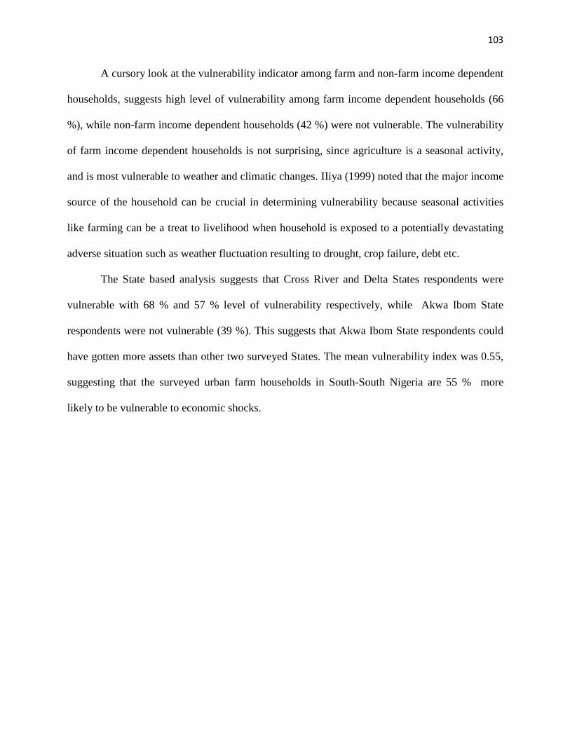
103
A cursory look at the vulnerability indicator among farm and non-farm income dependent
households, suggests high level of vulnerability among farm income dependent households (66
%), while non-farm income dependent households (42 %) were not vulnerable. The vulnerability
of farm income dependent households is not surprising, since agriculture is a seasonal activity,
and is most vulnerable to weather and climatic changes. IIiya (1999) noted that the major income
source of the household can be crucial in determining vulnerability because seasonal activities
like farming can be a treat to livelihood when household is exposed to a potentially devastating
adverse situation such as weather fluctuation resulting to drought, crop failure, debt etc.
The State based analysis suggests that Cross River and Delta States respondents were
vulnerable with 68 % and 57 % level of vulnerability respectively, while Akwa Ibom State
respondents were not vulnerable (39 %). This suggests that Akwa Ibom State respondents could
have gotten more assets than other two surveyed States. The mean vulnerability index was 0.55,
suggesting that the surveyed urban farm households in South-South Nigeria are 55 % more
likely to be vulnerable to economic shocks.
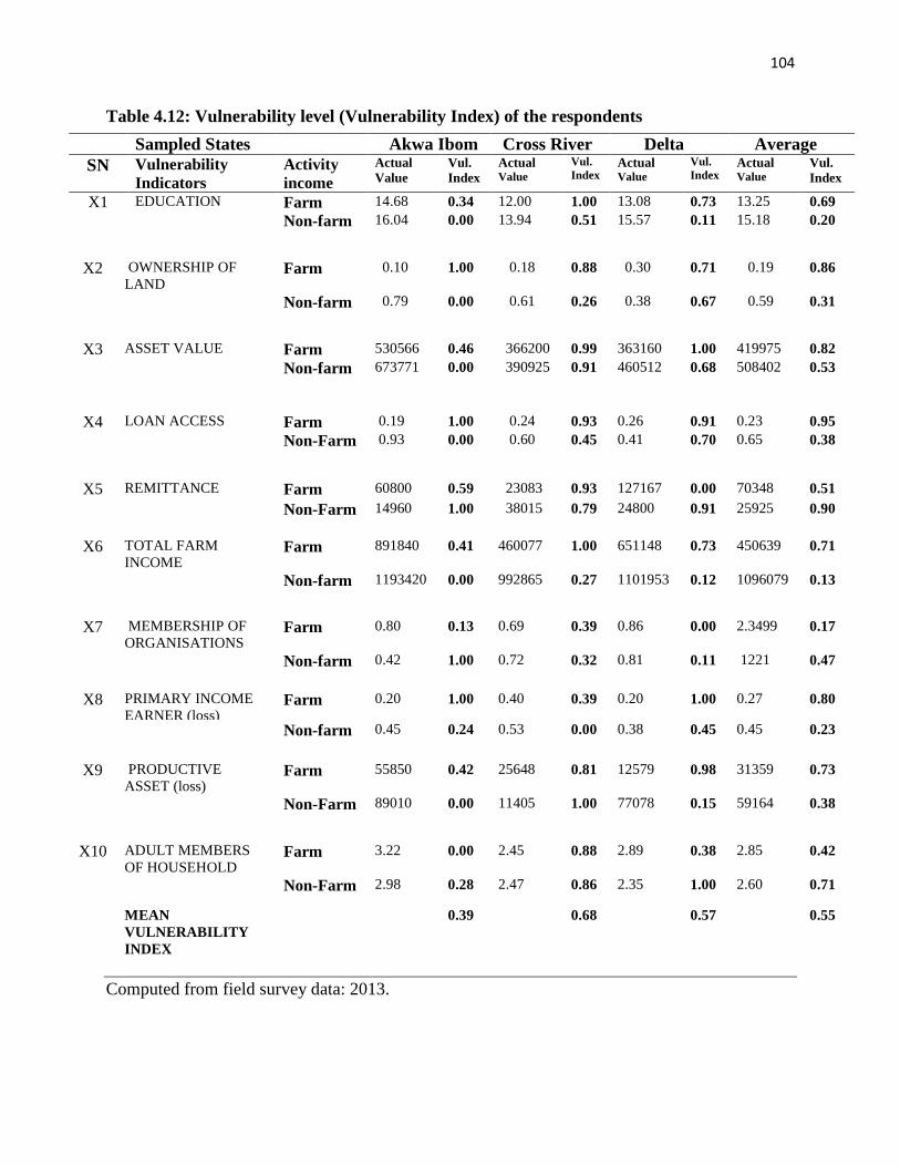
104
Table 4.12: Vulnerability level (Vulnerability Index) of the respondents
Computed from field survey data: 2013.
Sampled States Akwa Ibom Cross River Delta Average SN Vulnerability
Indicators Activity income
Actual Value
Vul. Index
Actual Value
Vul. Index
Actual Value
Vul. Index
Actual Value
Vul. Index
X1 EDUCATION Farm 14.68 0.34 12.00 1.00 13.08 0.73 13.25 0.69 Non-farm 16.04 0.00 13.94 0.51 15.57 0.11 15.18 0.20
X2 OWNERSHIP OF LAND
Farm 0.10 1.00 0.18 0.88 0.30 0.71 0.19 0.86
Non-farm 0.79 0.00 0.61 0.26 0.38 0.67 0.59 0.31
X3 ASSET VALUE Farm 530566 0.46 366200 0.99 363160 1.00 419975 0.82 Non-farm 673771 0.00 390925 0.91 460512 0.68 508402 0.53
X4 LOAN ACCESS Farm 0.19 1.00 0.24 0.93 0.26 0.91 0.23 0.95 Non-Farm 0.93 0.00 0.60 0.45 0.41 0.70 0.65 0.38
X5 REMITTANCE Farm 60800 0.59 23083 0.93 127167 0.00 70348 0.51
Non-Farm 14960 1.00 38015 0.79 24800 0.91 25925 0.90
X6 TOTAL FARM INCOME
Farm 891840 0.41 460077 1.00 651148 0.73 450639 0.71
Non-farm 1193420 0.00 992865 0.27 1101953 0.12 1096079 0.13
X7 MEMBERSHIP OF ORGANISATIONS
Farm 0.80 0.13 0.69 0.39 0.86 0.00 2.3499 0.17
Non-farm 0.42 1.00 0.72 0.32 0.81 0.11 1221 0.47
X8 PRIMARY INCOME EARNER (loss)
Farm 0.20 1.00 0.40 0.39 0.20 1.00 0.27 0.80
Non-farm 0.45 0.24 0.53 0.00 0.38 0.45 0.45 0.23
X9 PRODUCTIVE ASSET (loss)
Farm 55850 0.42 25648 0.81 12579 0.98 31359 0.73
Non-Farm 89010 0.00 11405 1.00 77078 0.15 59164 0.38
X10 ADULT MEMBERS OF HOUSEHOLD
Farm 3.22 0.00 2.45 0.88 2.89 0.38 2.85 0.42
Non-Farm 2.98 0.28 2.47 0.86 2.35 1.00 2.60 0.71
MEAN VULNERABILITY INDEX
0.39 0.68 0.57 0.55
105
Farm Income dependent household =0.66
Non- Farm Income dependent household =0.42
Overall vulnerability index = 0.55
The overall vulnerability index of 0.55 is an indication that urban farm households in South-
South Nigeria are likely to be vulnerable to economic shocks.
Figure 4.3 Bar chart showing vulnerability level of the respondents.
106
CHAPTER FIVE
SUMMARY, CONCLUSION AND RECOMMENDATIONS
5.1 Summary
As a long term solution to poverty and food insecurity problems in urban areas, farm
households need access to productive activities to generate more income. This is because the
urban environment is cash driven (intensive) and low incomes are likely to propel poor
households into food insecurity and poverty cycle. One way out is for such households to engage
in different income generating activities, using available households’ assets. By this, households
could exit poverty and food insecurity problems.
This study assessed the income generating activities among urban farm
households in South-South Nigeria using descriptive and inferential statistics. Six specific
objectives were developed to guide the study. Purposive, multi-stage and simple random
sampling techniques were employed in selecting 300 farm households from three (out of six)
States for the study. Out of the 300 copies of the questionnaire administered, 289 copies were
retrieved and used for the study. Data for the study were obtained from primary source using
structured questionnaires. Descriptive and relevant inferential statistics such as frequency,
percentages, mean, standard deviation, bar charts, ordinary least squares (OLS), Multinomial
logit (MNL) model, Quantile regression, and vulnerability analysis, were used for data analysis.
Based on the data analyzed from this study, majority (66%) of the household heads were
males while 34% were females. About (69%) of the respondents were between 31-50 years of
age, with the mean age of 44 years, and a standard deviation of 9.69. The bulks (77%) of the
household heads were in their active productive age range of less than 50 years. All the
respondents had some form of formal education. For instance, about 39% of the respondents had
107
at least secondary education. The remaining 61% had at least tertiary education with 15% of
them having Ordinary National Diploma (OND). Also, 14% had Higher National Diploma
(HND), 24% had Bachelor degree, while 8% had Masters degree. The average years of formal
education among the respondents was about 14 years, an indication that an average urban
farming household head was literate. The average household size of the respondent was about 5
persons. Greater percentage (44%) of the respondents had between 6-10 years of farming
experience while the average year of farming experience of the respondents was about 9 years.
Majority (93%) of the sampled respondents were once married, while about 7% never got
married.
Non-agric wage income was the most important income generating activity practiced by
about 36% of the household heads. Crop production income was the second most important
activity engaged by the sampled household heads (25% of the sampled respondent were
involved). About 19% of the respondents participated in income from other sources (trading,
bricklaying, and shoe making) as their major income generating activity. 14 % of the respondents
choose livestock income as their major income generating activity, while agricultural wage
income, income from pension, shares and rents, and remittance income were chosen by about
3%, 2% and 1% of the respondents respectively.
The results of the OLS estimates on the level of income generated by four income
generating categories showed that the models are quite reasonable compared to models in the
literature on total household income. The R2 were 0.61, 0.66, 0.29 and 0.55 for livestock income,
crop income, non-agricultural wage income and income from other sources respectively. This
implies that 61%, 66%, 29% and 55% of the variations in the livestock income, crop income,
non-agric wage income and income from other sources were explained by the independent
108
variables included in the model. The F–statistics of 0.0002 (5.40), 0.0000 (13.99), 0.0001 (4.32),
and 0.0000 (6.14) for livestock income, crop income, non-agric wage and income from other
sources respectively was significant at 1 percent critical value, suggesting that all the models
were of good fit.
Model 1 (livestock production model) showed that land size (p < 0.01) and asset value (p
< 0.01) positively and significantly influenced livestock production among the surveyed urban
farming households. Model 2 (crop production model) showed that while farming experience (p
< 0.01), land size (p < 0.01) and asset value (p < 0.01) positively and significantly influenced
crop production, the coefficient of household size (p < 0.05) had negative influence on crop
production. Suggesting that increasing household size reduces crop production income. Model 3
(non-agricultural wage income model), showed that educational level (p < 0.10) of household
heads and asset value (p < 0.01) significantly influenced non-agric. wage income among the
respondents. Model 4 (income from other sources) showed that educational level (p < 0.01) and
land size (0.05) significantly influenced income from other sources among the respondents.
On the socio-economic factors influencing choice of income generating activities among
the respondents. The multinomial logit analysis results showed that the coefficient of farm size
was statistically and significantly related to the probability that an urban farm household chooses
crop production (p < 0.01), livestock production (p < 0.01), and agricultural wage income (p <
0.01), as opposed to non-agricultural wage income. Also, the result of the marginal effect
indicates that an additional hectare of land ceteris paribus will result in a 12.6 %, 14.51 % and
1.2 % increase in the probability of household participating in Livestock income, Crop income
and Agric-wage income respectively as their major income generating activities.
109
The coefficient of gender had a negative and significant relationship with the probability
of a farm household choosing crop production as their major income generating activity. The
result of the marginal effect suggests that female headed households were about 36 % more
likely to choose crop production income as opposed to non-agricultural wage income. The
coefficient of adult household members in the household suggests that, having more adult
members in the household is positively related to the likelihood that household members would
partake in livestock or crop production as their major income generating activity. Also, number
of organizations in which the household heads belongs to, lead to an increased participation in
livestock production income. In addition, the marginal effect showed that being a member of one
additional social organization increased their participation in livestock production by 8.13
percent. Number of dependent in the household decreases the likelihood that an urban farm
household will partake in livestock production, agric. wage income, self-employed income and
other income sources.
A one year increase in years of formal education decreases the probability of the
household choosing livestock income, crop income and agricultural wage income by 0.06 %,
7.76 % and 0.04 % respectively, as opposed to non- agric wage income. A one unit increase in
age of household heads statistically increases the likelihood of the respondent choosing
remittance and other income sources as their major source of income. Also, a unit increase in
years of farming experience among household heads will results in a 0.44 %, 1.56 %, 0.19 % and
0.85 % increase in their probability of participating in crop income, agric. wage income and
income from other sources respectively as opposed to non-agricultural wage income. Marital
status coefficient had a negative relationship with farm income categories as opposed to non-
farm income categories. Meaning married households partook in non-farm income sources.
110
Analysis of the determinants of farm income among the surveyed urban farming
households suggests that, farmer’s age, gender, land size, assets value and non-farm income
positively and significantly influenced farm income. Conversely, educational level, farming
experience, marital status, household size, loan access and market proximity negatively and
significantly influenced farm income among the respondents.
Vulnerability analysis suggests that the urban farm households in the study area were
55% more likely to be vulnerable to economic shocks.
5.2 Conclusion
Urban farm household are engaged in different income generating activities to reduce
poverty and food insecurity problems. Households with large land sizes and high assets value
had more income from livestock production. In addition to large land size and high asset value,
households with more years of farming experienced and headed by female made more income
from crop production. Highly educated households, made more income from non-agricultural
wage and other income sources (although large land sizes also lead to increased income from this
category). Also, large land sizes, high asset value, years of farming experienced significantly
influenced households’ participation in crop production, livestock production and agricultural
wage income. Educational attainments significantly influenced households’ participation in non-
farm income generating activities.
Factors like, age of household heads, gender, land size, asset value, and non-farm income
positively and statistically influenced farm income. Conversely, farm location, years of formal
schooling, farming experience, marital status, household size, loan access, and market proximity
negatively and statistically influenced farm income. Urban farm household in the study area are
111
likely to be vulnerable to economic shocks. However, this study concludes that increasing urban
farm households’ productive assets strengthens household’s income generating capacities,
thereby ensuring tangible recoveries from economic shocks.
5.3 Recommendations
Based on the findings of this study, the following recommendations are made;
(a) Policy intervention strategies by international agencies, NGOs, private organizations and
government at all levels currently targeting rural farm households, should also focus on urban
farm households for sustainable development and achievement of millennium development
goals.
(b) Since land size positively influenced income generation, city planners and policy makers
should make effort to reclaim land which are unsuitable for building, as this will make land
available for agricultural production in the urban areas, thereby reducing food insecurity and
poverty.
(c) Asset value was statistically significant; the government at both State and local levels are
advised to establish a sustainable framework that will enable urban farmers access loan at
reduced interest rates. The provision of low interest capital will boost the acquisition of
productive assets which could increase household income, hence reducing their level of
vulnerability to economic shocks.
112
(d) Membership of organizations significantly influenced farm income. Urban farmers should be
encouraged to join more organizations (producer groups). Also, the capacities of existing
organizations/ producers group need to be strengthened.
5.4 Contribution to Knowledge
Many studies focused on rural development at the expense of urban dwellers, however,
this study focused on urban dwellers. The study indicated the socio-demographic factors that
influenced farm income among urban farmers of which farm location, years of formal schooling,
gender of household heads, marital status, household size, land size, access to loan, proximity to
market, asset value and non-farm income were found to be statistically significant. In addition,
the study showed the extent of vulnerability among urban farm households in the study area. The
identified factors are essential for the design of policies for promoting alternative income
generating activities, which will reduce poverty and food insecurity problems among urban farm
households. This is a significant contribution to knowledge for urban planners and policy makers
in agricultural development matters.
5.5 Suggestions for further Studies
Future researchers may focus on the following:
(i) A comparative study of Urban and Peri-urban farming in South-South Nigeria;
(ii) The impact of Urban agriculture on household food security in the study area;
(iii) Replicating this study in other geopolitical regions in Nigeria;
(iv) Efficiency of resource use among urban women farmers in South-South Nigeria; and
(v) Research on the extent of urban agriculture in Nigeria is necessary.
113
REFERENCES
Adams, R (2002). Non-Farm Income, Inequality and Land in Rural Egypt. Economic
Development and Cultural change 50 (2): 339-363
Adebayo, O.O. (2012). Family Income among Small-scale Farmers: A Panacea for food security
in Oyo State, Nigeria. Research on Humanities and Social Sciences. Vol. 2 no 7.
Adenegan, K. O., Adams, O., and Nwauwa, L. O. E.,(2013) Gender Impacts of Small-Scale
Farm Households on Agricultural Commercialisation in Oyo State, Nigeria. British
Journal of Economics, Management and Trade. Vol 3 no 1 pp 1-11
Adubi, A. A (1992). An Empirical analysis of production risk and attitudes of small farmers in Oyo State, Nigeria. Ph.D Thesis submitted to University of Ibadan, Nigeria.
African Development Bank (AfDB, 2012). Income inequality in Africa. Briefing notes for AfDB’s long-term strategy. Briefing number 5, 7th march.
Aina, O. S., Oladapo, A.,Adebosin, W. G. & Ajibola, S. (2012). “Urban Livelihood: Urban Agriculture Implication In Food: Case Study of Ibadan Metropolis”. Journal of Applied Hypotechnology in Environmental Sanitation, Vol. 1, Number 4.
Ajah, T. & Rana, H. (2005). “ Conceptualizing and Measuring Poverty as Vulnerability”: Does it make a different? ERD Policy Brief Series No. 41, Manila. Asian Development Bank.
Alayande, B. A & Alayande, O. (2004). A quantitative and qualitative assessment of vulnerability to poverty in Nigeria. A paper submitted for presentation of CSAE conference on poverty reduction, growth and human development in Africa, March.
Allingham, M. (2002). Choice Theory: A Very Short Introduction, Oxford: Oxford University Press.
Amaza, P., Tahorou, A., Patrick, K., & Amara, T., (2009). Changes in Househould Food Security and Poverty status in PROSAB areas of southern Borno State, Nigeria. Promoting Sustainable Agriculture in Bornu State (PROSAB). International Institute of Tropical Agriculture, Ibadan, Nigeria, pp 40.
Anderson, A. S.,(2002). Effect of Cash Cropping, Credit, and Household Composition on food Security in Southern Malawi. African Studies Quaterly, Vol. 6 no. 1&2.
Arene, C.J. & Mbata, G.I.O. (2008), ‘Determinant of profitability and willingness to pay for metropolitan waste-use in urban agriculture of the Federal territory, Abuja, Nigeria’, Journal of Tropical Agriculture, Food Environment and Extension, Vol 7, No 1,pp 41-46.
114
Armar-Klemeu M & Maxwell D. (2000). Accra: urban agriculture as an asset strategy, supplementing income and diets.
Armar-Klemesu, M. (2000) ‘Urban agriculture and food security, nutrition, and health’, in Growing Cities, Growing Food: Urban Agriculture on the Policy Agenda, German Foundation for International Development (DSE), Feldafing, Germany.
Ashley, C & Carney, D (1999). Sustainable livelihoods: Lessons from early experience. London: DFID.
Ashok K. Mishra, Hisham S. El-Osta, Mitchell J. Morehart, James D. Johnson & Jeffrey W. Hopkins (2002), Income,Wealth, and the Economic Well-Being of Farm households. Farm Sector Performance and Well-Being Branch, Resource Economics Division, Economic Research Service,U.S. Department of Agriculture. Agricultural Economic Report No. 812. Atamanov, A. (2011). Micro-economic analysis of rural non-farm activities in the Kyrgyz Republic: What determines participation and returns. Maastricht Graduate School of Governance, Maastricht University, The Netherlands. Azam, M. S & Imai, K. S (2012). Measuring Households Vulnerability to Idiosyncratic and Covariate Shocks- The case of Bangladesh. Being a discussion paper for Institute of Economics Economics and Business Administration. Kobe University Japan. Babatunde, R. O; Olagunju, F.I; Fakayode, S.B & Adejobi, A.O (2010). ‘Determinants of Participation in off-farm Employment among small-holder farming Households in Kwara State, Nigeria’. Production, Agriculture and Technology (PAT) Vol. 6(2) pp 1- 14. Babatunde, R. O & Qaim, I. (2010) “ Impact of off Farm Income on Food Security and Nutrition in Nigeria. Food Policy Vol. 35 pp 303-311. Barker, J. (2005). Survival and Accumulation Strategies at the Rural Urban Interface in North- west Tanzania. Rural Urban Linkages. Earthscan, London. Barret, A. & Reardon. (2000) ‘Poverty reduction in India: Towards building successful slum upgrading strategies.’Discussion paper for Urban Futures 2000 conference, Johannesburg.
115
Barret, C. B.; Reardon, T. & Webb, P (2001). Non-farm Income diversification and household livelihood Strategies in rural Africa: Concepts, Dynamics, and Policy implications. Food policy (26): 315- 331. Bebbington, A. (1999). Capitals and capabilities: A framework for analyzing peasant viability, rural livelihoods and poverty. World Development 27 (12): 2021–2044. Bennett, N. (2010). Sustainable Livelihoods from Theory to Conservation Practice: An Extended Annotated Bibliography for Prospective Application of Livelihoods Thinking in Protected Area Community Research. Protected Area and Poverty Reduction Alliance Working Paper No. 1. Victoria, Canada: MPARG (UVic); PAPR (VIU). Behrman, J. R. (1997). Intrahousehold distribution and the family. In Handbook of population and family economics, M. R. Rosenzweig and O. Stark, eds. The Netherlands: Elsevier Science. Borton, J. & Shoham, J. (1991). Mapping vulnerability to food insecurity: tentative guidelines for WFP offices. Study commissioned by the World Food Programme. London, UK, Relief and Development Institute. (Mimeo) Buechler, S. & Devi, G. (2002). Wastewater use for Urban Agriculture. Table handout during Hyderabad Conference, November. IWMI-IDRC (mimeo) Cade, B.S., Terrel,J.W., & Schroeder, R.L. (1999). Estimation effects of limiting factors with Regression Quantiles. Ecology 80:311-23 Calvo, C. & Davon, S. (2005). “ Measuring Individual Vulnerability”. Economic Series working Papers No. 229, Oxford, Department of Economics, University of Oxford. Campos, J., Ericsson, N. R. & Hendry, D. F., (1996). Cointegration tests in the presence of structural breaks. Journal of Econometrics, 70:187-220. Carney, D. (2003). Sustainable Livelihoods Approaches: Progress and Possibilities for Change. London: DFID. Carter, M. R & Barrett, C. B (2006). “The Economics of Poverty Traps and Persistence Poverty”. Journal of Development Studies. No. 2 pp 178-199. Central Intelligence Agency (CIA) (2012). The world fact book. Retrieved 10th April 2013 from http//www.CIA.gov/library.
116
Chambers, R, Pacey, A, & Thrupp, L.A (eds) (1989). Farmer first: Farmer innovation and agricultural research. Intermediate Technology Publications, London.
Chambers, R. & Conway, R. (1992) ‘Sustainable rural livelihoods: Practical concepts for the 21st century’, Institute of Development Studies (IDS), Brighton, UK, Discussion Paper
Chambers, R. (1997), “Whose Reality Counts: Putting the Last First”. Intermediate Technology Publications No. 296
Chant, S (2013). Cities through a “Gender Lens”; a golden “urban Lens” for women in the global South. Environment and Urbanization Vol. 25, No 1, April.
Chaudhuri, S. (2003). “Assessing Vulnerability to Poverty: Concepts, Empirical Methods, and Illustrative Examples”. Mimeo, Columbia University.
Chaudhuri, S., J. Jalan, & A. Suryahadi. (2002). Assessing household vulnerability to poverty: A methodology and estimates for Indonesia. Department of Economics Discussion Paper No. 0102-52. New York: Columbia University.
Chen, C., Amwei, Y. (2005). Computational Issues on Quantile regression. Special issue on quantile regression and related methods. Sankhya. Forthcoming .
Christiaensen, L (2004): Measuring Households Vulnerability: Conceptual issues and illustrative examples. PADI conference on Measuring, Understanding and Alleviating Households Vulnerability, Dar es Salaam, 2-3 February. World Bank.
Christiaensen, J., & Subbarao, K. (2004). Toward an understanding of household vulnerability in rural Kenya. World Bank Policy Research Working Paper 3326. Washington D.C: World Bank.
Chukwuone, N.A. (2009). “Analysis of Conservation and Utilization of Non-Wood Forest Products in Southern Nigeria: Implications for Forest Management and Poverty Alleviation”. A Ph.D Thesis Submitted to the Department of Agricultural Economies, University of Nigeria, Nsukka.
Corel, L & Reardon, T (2001): Rural non- farm income in Nicaragua: World Development. 29 (3): 427-442.
Cornia, G. A. (1987) “Adjustment at the household Level: potential and Limitations of Survival Strategies” in Cornia, Jolly and Stewart (eds). Adjustment with Human Face, UNICEF, Claredon press, Oxford.
117
Dasgupta, P. (1993) An Inquiry into Wellbeing and Destitution. Oxford: Claredon Press.
Deaton, A. (1997). The Analysis of Household Surveys. Baltimore: The John Hopkins University Press.
Deere, C. D., & Doss, C. (2006). The Gender Asset Gap: What do we know and why does it matter? Feminist Economics 12(1–2): 1–50.
Deressa, T. T; Hassan, R. M & Ringler, C. (2009). Assessing Household Vulnerability to Climate Change: The Case of Farmers in the Nile Basin of Ethiopia. Washington DC: International Food Policy Research Institute (IFPRI).
de Janvry, A & Sadoulet, E (2001). Income Strategies amoung Rural households in Mexico: the role of off-farm activities. World Development report. 29(3) : 467-480
de Janvry, A., Sadoulet, E., & Zhu, N., (2005). The Role of Non-Farm Incomes In reducing Poverty and Inequality in China. CUDARE working paper 1001, University of Califonia, Berkeley.
de Sherbinin, A., Vanwey, L.K., McSweeney, K., Aggarawal. R., Barbieri, A, Henry, S., Hunter, L.M., Twine, W., Walker, R., (2008). Rural household demographics, livelihoods and the Environment. Global environmental Change, 18. 38-53
Department for International Development DFID. (2001) Sustainable Livelihoods Guidance sheets. <www.livelihoods.org/info/info_guidanceSheets.html#6> (accessed September 2012).
Diebold, F. X. & Chen, C., (1996). Testing structural stability with endogenous breakpoint – A size comparison of analytic and bootstrap procedures. Journal of Econometrics, 70:221-241. Drakakis-Smith, D. (1997), ‘Third world cities: sustainable urban development 111 – basic needs and human rights’, Urban Studies, Vol 34, Nos 5–6, pp 797–323.
Drechsel P. & Dongus, S. (2010). Dynamics and sustainability of urban agriculture: examples from sub-Saharan Africa. Sustain. Sci., 5(1): 69-78.
Drescher A. (1996). Management strategies in African homegardens and the need for new extension approaches. In: Heidhues F & Fadani A (eds), Food security and innovations: successes and lessons learned (Frankfurt: Peter Lang).
Drescher, A.W. (2001), ‘The integration of urban agriculture into urban planning – an analysis of current status and constraints’, in Annotated Bibliography on Urban Agriculture, ETC Urban Agriculture Programme & Swedish International Development Agency (SIDA),
118
Leusden, The Netherlands, accessed 20 September 2011 from website: http://www.rauf.org/bibliography/annotated/html.
Drescher, A.W. (2002), ‘Urban and peri-urban agriculture and urban planning’, a paper contributed to the Electronic Conference on Urban and Peri-urban Agriculture, RUAF, accessed 21 October 2007 website: http:// www.fao.org/urbanag/paper/_enhtm.
Eboh, E. C. (2009). Developing Conceptual Framework for Empirical Research. In Anyakoha, E. U. (Ed) Developing Research Skills: Concepts and Conceptual Frameworks. Nsukka: Great AP Express Publishers Ltd.
Egbuna, N. E. (2008). Urban Agriculture: A strategy for Poverty Reduction in Nigeria. CBN Abuja, Nigeria.
Ellis. F. (1992). Peasant Economics. Cambridge: Cambridge University Press.
Ellis, F.(1998). Household Strategies and Rural Livelihood Diversification, Journal of Development Studies, vol. 35:1, 1-38.
Ellis, F (2000). Determinants of Rural Diversification in Developing Countries. Journal of Agricultural Economics 51 (2): 289-302
Ellis, F. & Freeman, H.A. (2004): Rural Livelihoods and Poverty Reduction Strategies in Four African Countries, Journal of Development Studies, 40:4, 1-30.
Enete, A.A. (2003). “Resource Use, Marketing and Diversification Decisions in Cassava Producing Household of Sub-Saharan Africa”. A Ph.D Dissertation Presented to the Department of Agricultural Economics, Catholic University of Louvain, Belgium.
Etim, N. A., & Ukoha, O.O (2010). Analysis of poverty profile of rural households: evidence from South-South Nigeria.
Ezedinma, C. & Chukuezi, C (1999). A comparative analysis of urban agriculture enterprises in Lagos and Port Harcourt, Nigeria. Environment and Urbanization, 11(2): 135-144.
Fafchamps, M. &. Quisumbing, A. R. (2002). Control and ownership of assets within rural Ethiopian households. Journal of Development Studies 38(2): 47-82.
Farmer, B. H. (1977). Green revolution? Technology and Change in Rice-Growing Areas of Tamil Nadu and Sri Lanka. Boulder, Colorado: Westview Press. Retrieved November 22, 2012, from http://www.cababstractsplus.org/abstracts%5C/Abstract.aspx?AcNo=19776.
Ferreira, F. H.G, Lanjouw, P., (2001). Rural non-farm activities and poverty in the Brazillian Northeast. World Development, 23 (3) 509-528
Fishburn, P. C. (1968). Utility Theory. Management Sciences. 14 (5): 335 – 378.
119
Food & Agricultural Organization (FAO), 1999, Issues on urban agricultural retrieved 8th December 2011 from FAO Website: http://www.fao.org/ag/magazine19901sp2.htm
Food & Agricultural Organization (FAO). (2001). A briefing guide for the successful implementation of urban and peri-urban agriculture in developing countries and countries of transition. Revision 2, Handbook Series. Volume III.Rome
Food & Agricultural Organization (FAO), WFP & IFAD (2012). The State of Food Insecurity in the World. Economic Growth is Necessary but not Sufficient to Accelerate Reduction of Hunger and Malnutrition. Rome, Food and Agricultural Organization.
Frankenberger, T. (1996). Measuring household livelihood security: an approach for reducing absolute poverty. Food Forum, No. 34. Washington, DC, USA.
Foeken, D. & Mboganie M, A. (2000). Increasing food security through urban farming in Nairobi. In N. Bakker, M. Dubbeling, S.Guendel, U. Sabel Koschella & H. de Zeeuw, eds. 2000. Growing cities, growing food, urban agriculture on the policy agenda, pp 303–328. DSE, Feldafing.
Gaiha, R., & Imai, K. (2004). Vulnerability, persistence of poverty and shocks – estimates for semi-arid rural India. Oxford Development Studies 32, no 2: 261-81
Gefu, J. O. (1992) “ Part-time Farming as an Urban Survival Strategy: A Nigerian Case Study: in Barker, J & Pendersen, P. O. (Eds). The Rural Urban Interface in Africa: Expansion and Adaptation, Nordiska Afrikainstitute, Uppsala.
Goldman, I, Franks, T, Toner, A, Howlett, D, Kamuzara, F, Muhumuza, N & Tamasane, T (2004). Goodbye to projects: Application of sustainable livelihood principles. http://www.brad.ac.uk/acad/dppc/GTP/goodbye.html. Accessed on October 2012.
Greene , W. H., (2003) Econometric Analysis. London: Prentice Hall.
Grootaert, C. (1999). Social Capital, Household Welfare and Poverty in Indonesia. Washington D.C. The World Bank.
Haddad L; John H. & Harold A. (1997). Intra-household Resource Allocation in Developing Countries, Johns Hopkins University Press, Baltimore. Haddad L, Ruel M, & Garrett, J. (1997). Growing Urban Poverty and Undernutrition and some
Urban Facts of Life: Implications for Research and Policy. Washington, DC: International Food Policy Research Institute.
Hassen, E. K (2008). Fighting poverty in South Africa: A civil society. http://www.naledi.org. Accessed on 2012-05-02.
120
Henn, P. (2002). User benefits of urban agriculture in Havana, Cuba: An Application of the Contingent Valuation Method. Available at http://www.cityfarmer.org/havanaBenefit.html [accessed on 23 September 2012].
Hinshelwood, E. (2003). Making friends with the sustainable livelihoods framework. Community Development Journal, 38(3), 243-254.
Hoddinott, J., & Quisumbing, A, (2003). Methods for microeconometric risk and vulnerability assessments. Social Protection Discussion Paper Series No. 0324. Social Protection Unit, Human Development Network. Washington D.C: World Bank.
Hoffman, T and Ashwell, A. (2001). Nature Divided: Land Degradation in the South Africa. Cape Town: University of Cape Town Press.
Holzmann, R. & Jorgensen, S (2000). “Social Protection as Social Risk Management:
Conceptual Underpinnings for the Social Protection Sector Strategy Paper”. Journal of International Development, vol. 1, 1005-27.
Hussein, K. (2002). Livelihoods Approaches Compared: A Multi-Agency Review of Current Practice. London, UK: DFID.
Hutcheson, G. D. (2011). Ordinary Least-Squares Regression. In L. Moutinho and G. D. Hutcheson, The SAGE Dictionary of Quantitative Management Research. Pp 224-228.
IIiya, M. A. (1999). Income Diversification in Semi-arid zone of Nigeria: A study of Gigane, Sokoto, North-west Nigeria. ASC working paper, vol. 39. Kano: center for research and documentation (CRD) and Leiden: African Studies center.
International Food Policy Research Institute. IFPRI (2007). Pathways from poverty: A proposal for a global research program (GRP26). Washington, DC: International Food Policy Research Institute.
Jedwab, R. (2012).“Why Is African Urbanization Different? Evidence from Resource Exports in Ghana and Ivory Coast. http://home.gwu.edu/~jedwab/JEDWAB_JMP_14112011 pdf.
Kessler, A. (2003). Economic strategies of different plant production farming systems of urban and peri-urban agriculture in West Africa. Urban Agriculture Magazine, no 7. August, Economics of urban agriculture. Leusden, The Netherlands, RUAF.
Koenker, R. (2005). Quantile Regression. Cambridge University Press.
Koenker, R. & Basset, G. W. (1978), “Regression Quantiles” Econometrica,vol. 46, pp 33-50.
Koenker, R & Hallock, K (2001), “Regression Quantiles: An introduction” Journal of Economic perspective, vol. 15,no 4 pp 143-156.
121
Kozumi, H. & Hasegawa, H., (2000). A Bayesian analysis of structural chances with an application to the displacement effect. The Manchester School of Economic and Social Studies, 68:476- 490. Le Breton, S. & Brusati (2001). A review study on HIV and labour interface: save the children Lerman & McKernan (2008). The Effects of Holding Assets on Social and Economic Outcomes
of Families: A review of Theory and Evidence. The urban Institute Center for Social Development. Washington University. http//aspe.hhs.gov/hsp/.
Ligon, E., & L. Schechter. (2003). Measuring vulnerability. Manuscript. California: University of California, Berkeley.
Lipton, M. (1968). Theory of Optimizing Peasant. Journal of Development studies. 4 (3): 327-51
Lipton, M., & Moore, M. (1972). The Methodology of Village Studies in Less Developed Countries. Brighton: IDS,University of Sussex.
Loevinsohn, M., & Gillespie, S. (2003). HIV/AIDS, Food Security and Rural Livelihoods. FCND Discussion Paper 157. International Food Policy Research Institute (IFPRI). Retrieved November 22, 2012, from http://ideas.repec.org/p/fpr/fcnddp/157.html
Long, N. (1984). Family and Work in Rural Societies: Perspectives on Non-Wage Labour. London; New York: Tavistock.
Longley, C., & Maxwell, D. (2003). Livelihoods, Chronic Conflict and Humanitarian Response: A Synthesis of Current Practice. Working Paper 182. London: ODI.
Ludi, E & Slater, R (2008). Using Sustainable Livelihood Framework to Understand and Tackle Poverty. Working paper. London: ODI
Manser, M., & Brown, M. (1980). Marriage and household decision making: A bargaining analysis. International Economic Review 21: 31–44.
Marenya, P. P. & Barrett, C. B. (2007). Household Level Determinants of Adoption of Improved Natural Resource Management Practices among Smallholder farmers in Western Kenya. Food Policy 32: 515-536.
Martey, E., Al-Hassan, R.M., & Kuwornu, J.K.,(2012). Commercialization of smallholder agriculture in Ghana: A Tobit regression analysis. African Journal of Agricultural Research, 7(14), 2131-2141.
Martin, A., Oudwater, N. & Meadows, K. (2000) ‘Urban agriculture and the livelihoods of the poor in Southern Africa: Case Studies from Cape Town and Pretoria, South Africa and Harare, Zimbabwe’, Paper presented at the International Symposium ‘Urban agriculture
122
and horticulture: the linkage with urban planning’, 7–9 July 2000, Berlin, Germany. Sponsored by TRIALOG, Vienna, Austria; Humboldt-University, Berlin, Germany; HABITAT, Havana, Cuba.
Mathenge, M., Place, F., Olwande, J., & Mithofer, D., (2010). Participation in Agricultural markets among the poor and marginalized: Analysis of Factors Influencing Participation and Impacts on Income and Poverty in Kenya.Teemeo institute. Egerton University, Kenya.
Matshe, I. & Young, T. (2004) Off-farm Labor Allocation Decisions in Small Scale Rural Households in Zimbabwe. Agricultural Economics, 40 (2): 175-186
Mattila-wiro, P. (1999). Economic theories of Household: A critical review. Issue 159 WIDER working paper. World institute for Development Economics Research.
Maxwell, D (1995) Alternative food Security Strategy: A household analysis of Urban Agriculture in Kampala. World Development 23(10): 1669-1681
McElroy, M. B. & Horney, M. J (1981). Nash-bargained household decisions: Toward a generalization of the theory of demand. International Economic Review 22: 333–49.
McGee, T. (2006). Constructal Theory: Sustainability. Retrieved December 10, 2012 from http://www.treehugger.com/about?.
McNally, R. & Othman, M. S. (2002). Environmental Economics: A practical Guide. Malaysia, WWF – UK.
Meng, T, Florkowski, J. W, Sarpong, D., Resurreccion, A. V, Chinnan, M (2013). The Determinants of Food Expenditure in Urban Households of Ghana: A Quantile Regression Approach. A Paper presented at the Southern Agricultural Economics Association (SAEA) annual meeting, Orlando, Florida, 3-5 February.
Meikle, S., Ramasut, T. & Walker, J. (2001). Sustainable Urban Livelihoods: Concepts and Implication for Policy. Working Paper No. 112.
Meinzen-Dick, R., N. Johnson, A. Quisumbing, J. Njuki, J. Behrman, D. Rubin, A. Peterman, and E. Waitanji (2011). Gender, Assets, and Agricultural Development Programs: A Conceptual Framework. CAPRi Working Paper No. 99. International Food Policy Research Institute: Washington, DC. http://dx.doi.org/10.2499/CAPRiWP99.
Mishra, A. K. & Holthausen, D. M. (2002). Effect of farm income and off-farm wage variability on off-farm labour supply. Agricultural and Resource Economics Review, 31 (2), 187- 199
123
Moock, J. (1986). Understanding Africa's Rural Households and Farming Systems. Boulder: Westview Press.
Morduch, (1994) “Poverty and Vulnerability” American Economic review vol.84, no 2, pp 221- 225
Morduch, (1995) “ Income Smoothing and Consumption Smoothing” Journal of economic Perspectives. Vol. 9, No. 3 pp 103-114
Moser, C. (1998). Confronting Crises: “A Comparative Study of Household Responses to Poverty and Vulnerability in Four Urban Communities”. ESD. Washington.
Mougeot, L. (2000) ‘Urban agriculture: definition, presence, potentials and risks’, in Bakker, N., Dubelling, M., Gründel, S., Sabel-Koschella, U. and de Zeeuw, H. (eds) Growing Cities, Growing Food. Urban Agriculture on the Policy Agenda, German Foundation for International Development (DSE), Feldafing, Germany.
Mukundi, E., Mathenge, M., & Ngigi, M (2013). Sweet potato Marketing among small-holder farmers: The role of collective action. Invited paper presented at the 4th International conference of the African Association of Agricultural economist, September 22-25, Hammamet, Tunisia.
Musyoki, J.K., Mugwe, J., Mutundu, K., & Muchiri, M., (2013). Determinants of Household Decision to join community Forest Associations: A case Study of Kenya. ISRN Forestry.
Myers, B. (1999). Walking with the poor. New York: Orbis.
Narayan, D., with R. Patel, K. Schafft, A. Rademacher, & S. Koch-Schulte (2000). Voices of the poor: Can anyone hear us? New York: Oxford University Press for the World Bank.
Narayan, D, & Pritchette, L. (1999). Cents and Sociability: Household Income and Social Capital in Tanzania in Economic Development and Cultural Change 47(4), 871–897.
National Bureau of Statistics. NBS (2012). Press briefing by the Statistician-General of the Federation/ Chief Executive officer; National Bureau of Statistics (NBS) on the Nigerian Poverty profile. 2010/ 2011. Abuja, Nigeria.
National Population Commission. NPoC (2006) National Population Census, Federal Republic of Nigeria official gazette, Lagos, Nigeria.
Ninno, C. D. & Marini, A. (2005): Household’s Vulnerability to Shocks in Zambia. Special protection Discussion Paper No. 0536, World Bank.
124
Nkegbe, P. K. (2002) Benefit Costs analysis of Irrigated Vegetable Production in Urban and Peri-urban Tamale. University of Development Studies, Ghana.
Nugent, R. (2000) ‘The impact of urban agriculture on the household and local economies’, in Bakker, N., Dubelling, M., Gründel, S., Sabel-Koschella, U. and de Zeeuw, H. (eds) Growing Cities, Growing Food: Urban Agriculture on the Policy Agenda, DSE, Feldafing, Germany.
Oduh, M.O. (2012). The Dynamics of Poverty and Income Distribution: Is the Nigerian Middle Class Statistically or Economically growing? Developing Countries Studies, Vol. 2, No.7.
Odion, W. E. (2009). Millennium Development Goals (MDGs) and the Poverty Questions in Nigeria. in Omotor, D. G and Akpotor, A. S. (eds) Millennium development Goals and Challenges Abraka: Delsu Investment Nigeria Ltd.
Okon, U. E & Enete, A. A. (2009). Resource Use Efficiency among Urban Vegetable farmers in Akwa Ibom State, Nigeria. Tropicultura, Vol. 27, No. 4.
Okon, U. E., Enete, A. A. & Amusa, T. A. (2012): Enterprise Choice Decisions in Urban Food Production in Nigeria: Empirical evidence from Akwa Ibom State. Outlook on Agriculture Vol. 41, No 1, Pp 51-56.
Okorji, E. C (1988). Women and Rural development Strategies for sustaining Women contribution in Rural Households of Anambra State, Nigeria. Working paper No 166. Women in International Development, Michigan State University, pp 16.
Okorji, E. C., Okon, U. E., Nwankwo, J. O. (2012). Socio-economic Determinants of Irrigated Vegetable Production Systems in Anambra Agricultural Zone of Anambra State, Nigeria. Nigerian Agricultural Journal vol. 43
Okunmadewa, F.Y, Yusuf, S. A., Omonoma, B. T. (2007). Effects of Social Capital on rural Poverty in Nigeria. Pakistan Journal of Social Sciences 4(3): 331-339
Olowookere, S. (2010). Sustainable Agriculture. Retrieved December 10, 2012 from http://www.education.ezinemark.com
Osawe, O.W., (2013). Livelihood vulnerability and migration decision making nexus: The case of rural farm households in Nigeria. Invited paper presented at the 4th International conference of the African Association of Agricultural economist, September 22-25, Hammamet, Tunisia.
125
Oseni, G. & Winter,P (2009) “ Rural no-farm Activities and agricultural crop Production in Nigeria. Agricultural Economics, Vol. 40 pp 189-20.
Otieno, D. J., Omiti, J. Nyanamba, T. & McCullough, E. (2009). Application of Chow test to Improve Farmer Participation in Markets in Kenya. A contributed paper prepared for presentation at the 27th Conference of the International Association of Agricultural Economist (IAAE), 16th -22nd August, Beijing, China.
Owuor, G., (2009). Can Group Based Credit Uphold Smallholders Farmers Productivity and Reduce Poverty in Africa? Empirical Evidence from Kenya. Seminar paper presented at 111 EAAE-IAAE Seminar 26th -27th June, University of Kent, Canterbury, United Kingdom.
Pablo, D. & Miguel, T. (2005). A Multinomial Logit Econometric Model of the Factors Influencing the adoption of environmental technologies in the Pulp and Paper sector in Spain. International Journal of Envoronmental Technology and Management Vol. 5(4), Pp 28.
Panda, P. & Agarwal, B. (2005). Marital violence, human development and women’s property status in India. World Development 33(5): 823–850.
Pandya, Y (2012). Urban Agriculture: Growing green in grey concrete. Agency: DNA (Daily News and Analysis) http:/www.dnaindia.com/analysis/column_urban-agriculture- growing-green-in-grey-concrete. Assessed 11th September,2013.
Phillips, D., Williams, K., Andrews, G., Clarke, J., Carter, M., Kinsman, P.,Smith, D., Willis, K., Bradbury,I.,Wu, K. & Hillyer, A. (1999): Literature Review on Peri-Urban Natural Conceptualization and Management Approaches, Final Technical Report, DFID Natural Resource Systems Programme (NRSP), Project R6949, University of Nottingham and University of Liverpool.
Phillips, D & Rayhan, M (2004). Vulnerability and Poverty: What are the causes and how are they related? International Doctoral Studies, center for development research; University of Bonn, Germany.
Qasim, M. (2012) Determinants of Farm Income and Agricultural Risk Management strategies. The case of Rainfed Farm Households in Pakistan’s Punjab. International Rural development, vol. 3.
Rakodi C. (2002). A livelihood approach- conceptual issues and definitions. In Urban Livelihoods: A People-Centred Approach to Reducing Poverty, Rakodi C, Lloyd-Jones T (eds).Earthscan Publications: London.
126
Rakodi C. (1995). The household strategies of urban poor: coping with poverty and recession in Gweru, Zimbabwe. Habitat International 19 (4): 447–471.
Reardon, T. (1997). Using Evidence of Household Income Diversification to inform study of the rural nonfarm labor market in Africa. World Development 25 (5): 735-748.
Reardon, T. Berdegué, J. Barrett, C. B. & Stamoulis, K,(2006). Household Income Diversification into Rural Nonfarm Activities. In S. Haggblade, P. Hazell and T. Reardon (Eds.), Transforming the Rural Nonfarm Economy. Baltimore: Johns Hopkins University Press.
Reardon, T. & S. Vosti, (1995). Links between rural poverty and the environment in developing countries: Asset categories and Investment Poverty. World Development, 23(9): 1495- 1506.
Resource Centers on Urban Agriculture and Food Security [RUAF Foundation] (2007), ‘Why urban agriculture is important’, accessed 18 December 2011 from website: http://www.ruaf.org.
Rougoor, C. W., Ruud, B. M., Huirne, & Renkema (1998). How to define and study farmers’ management capacity: Theory and use in Agricultural Economics. Agricultural Economics, 18: 261-272
Roumasset, J. (1976). Rice, Risk: Decision Making among Low-Income Farmers. North-Holland, Amsterdam. North-Holland Publishing.
Sabates R, Gould B.W, & Villarreal, H.J. (2001). Household composition and food expenditures: A Cross Country Comparison. Food Policy 26: 571–586.
Salafky, N. & Wollenberg, (2000) linking livelihoods and Conservation: A conceptual framework and Scale for Assessing the Integration of human needs and Biodiversity. World development 28 (8)
Sanderson, D. (2000) Cities, Disasters and Livelihoods, CARE, United Kingdom. Also available at www.livelihoods.org/cgi-bin/dbtcgi.exe (accessed 20 November 2011)
Sanyal B. (1985). Urban agriculture: who cultivates and why? Food and Nutrition Bulletin 7 (3): 15–25.
Satterthwaite, D. (1995) ‘Urban poverty: Reconsidering its scale and nature’. IDS Bulletin 28 (2). Brighton, UK: Institute of Development Studies, University of Sussex.
127
Satterthwaite, D. (2000) ‘Seeking an understanding of poverty that recognises rural–urban differences and rural–urban linkages.’ Paper presented at the World Bank’s urban forum on Urban Poverty Reduction in the 21st Century, International Institute for Environment and Development (IIED), April.
Satterthwaite, D., Huq, S., Pelling, M., Reid, H. & Lankao, P. R ( 2007). Adapting to Climate Change in Urban Areas: The possibilities and constraints in low- and middle-income nations. IIED Human Settlements Discussion Paper Series. Retrieved from www.iied.org/pubs/display.php on Oct 31, 2012.
Scoones, I. (1998). Sustainable Rural Livelihoods: A Framework for Analysis. IDS Working Paper 72. Sussex: IDS,University of Sussex
Scoones, I. (2009). Livelihoods perspectives and rural development. Journal of Peasant Studies, 36(1), 171-196.
Sen, A. (1999) Development as Freedom. Anchor Books, New York. Retrieved 18th June 2013 from http//www.ocean.otr.usm.edu.
Sesabo, J. K & Tol, R. S (2005). Factors affecting Income Strategies among household in Tanzanian Coastal Villages: Implication for Development conservation initiatives. Research unit sustainability & Global Change. Humburg University and Center for Marie and Atmospheric science. Working Paper FNU- 70.
Shahan, Z. (2009). What is Sustainability? The Practice Makes the Ideal, the Critical 4th Component. Retrieved December 10, 2012 from http://www.blog.sustainablog.org/
Simpson, M. C. (2007). An integrated approach to assess the impacts of tourism on community development and sustainable livelihoods. Community Development Journal, 44(2), 186- 208.
Singh, N. & Gilman, J. (1999) ‘Making livelihoods more sustainable’, International Social Science Journal, vol 51, no 4, pp539–545
Skoufias, E. (2003). Consumption smoothing in Russia. Economics of Transition 11(1): 67–91.
Smit J. (1996). Urban agriculture – food jobs and sustainable cities. United Nations Development Programmes: New York.
Solow, R. M. (1991), Sustainability: An Economist Perspectives. A Paper presented at the eighteenth J. Seward Johnson Lecture to the Marine policy center. Woods Hole Oceanographic Institution, Massachussetts, June 11.
128
Stratton, L.S., D.M, O’toole & J.M, Wetzel. (2003). “A Multinomial Logit Model of Attrition That Distinguishes Between Stopout and Dropout Behaviour.” Retrieved June 14, 2012, from http:// www.eric.ed.gov/
Strauss, J & Thompson, D (1995). Human Resources: Emperical modelling of Household and Family Decisions. In Berhman, J & Srinivasan, T. N (eds). Hand Book of development Economics.
Tacoli, C. (1998) ‘Rural–urban linkages and sustainable rural livelihoods’ in Carney, D (ed.) Sustainable rural livelihoods. London: Department for International Development, HMSO
Tacoli, C. (2002), Changing rural-urban interactions in sub-Saharan Africa and their impact on livelihoods: a summary. Working Paper Series on Rural-Urban Interactions and Livelihood Strategies: Working Paper 7. London: International Institute for Environment and Development (IIED)
Taruvinga, A. & Mushunje, A., (2010). Socio-economic factors that influence households’ participation in wetland cultivation: A binary logistic regression of wetland cultivators and non-cultivators. Paper presented at the Joint 3rd African Association of Agricultural Economics (AAAE) and 48th Agricultural Economist Association of South Africa (AEASA) Conference, Cape Town, South Africa, September 19-23.
Taylor, J. E., & Yunez-Naude, A. (2000). The returns from Schooling on a Diversified Rural Economy. American Journal of Agricultural Economics vol. 82, 287-297.
Terrel, J. W., Cade, B. S., Carpenter, J., & Thompson, J. M., (1996). Modelling Stream Fish habitat limitations from wedged-shaped patterns of variation in standing stock. Trans Am fish soc 125: 104-17
Thomas, D.;Contreras, D & Frankenberg, E. (2002). Distribution of power within the household and child health. Mimeo. Santa Monica, CA: RAND.
Umoh, G.S. (2006), ‘Resource use efficiency in urban farming: an application of stochastic frontier production function. International Journal of Agriculture and Biology, Vol 8, No1, pp 37–44.
United Nations Human Settlement Programme (UN-Habitat, 2012).
United Nations (2008). World urbanization prospects: the 2007 revision. United Nations, Department of Economic and Social Affairs, Population Division, New York. http://esa.un.org/unup.
129
United Nations Center for Human Settlements, UNCHS (1996), An Urbanizing World: Global Report on Human Settlements. London: Oxford University Press (for United Nations Centre for Human Settlements).
United Nations Population Fund (2007). The State of the World Population. United Nations Population Fund, (UNPF) New York. http://www.unfpa.org/swp/2007
United Nations Development Programme (1996), Urban Agriculture: Food, Jobs and Sustainable Cities, United Nations Development Programme (UNDP), New York.
United Nations Development Programme (1997) Human Development Report, Oxford University Press.
United Nations Development Programme (1997). Governance for Sustainable Human Development. New York. ‘Developing SL indicators: Reviewing lessons learned and a framework for action.’UNDP (http://www.undp.org/).
United Nations General Assembly, (2010). Progress to date and remaining gaps in the implementation of the outcomes of the major summits in the area of sustainable development and analysis of the themes for the Conference: Report of the Secretary- General. The Preparatory Committee for the United Nations Conference on Sustainable Development, 17-19 May.
United Nations (2006), World Urbanization Prospects – The 2005 Revision, Department of Economic and Social Affairs, United Nations Population Division, New York.
Van Veenhuizen, R. (2006), ‘Cities farming for the future’, in Van Veenhuisen, R., ed, Cities Farming for the Future: Urban Agriculture for Green and Productive Cities, RUAF Foundation, IIRR, IDRC, Ottawa, Canada, pp 1–17.
Variyam, J. N., Blaylock, J., & Smallwood, D. (2002). Characterising the Distribution of Micro- nutrient Intake among US adults: A quantile regression approach. American Agricultural Economics, 84 (2), 454- 466.
Vaughan, C., & Katjiua, J. (2003). An Overview of Community Based Natural Resources Management and Rural Livelihoods in Khoadi/Haos Conservancy - Kunene Region. Wildlife Integration for Livelihood Diversification (WILD)
Walker, T., & Jodha, N. (1986). “How Small Farmers adapt to risk”. In P. Hazell, C. P. Mareda, and Valdez, eds., Crop insurance for agricultural development. Baltimore: John Hopkins University press.
Wanyama, M; Mose, L.O; Okuro, J; Owuor, G. S & Mohammed, L (2010) ‘Determinant of income diversification Srategies amongst Rural Households in Maize based farming systems of Kenya. African Journal of Food Science, vol. 4(12) pp 754-763.
130
Whitehead, A. (2002). Tracking livelihood change: Theoretical, Methodological and Empirical Perspectives from North-East Ghana. Journal of Southern African studies, Volume 28 (3), pp : 573-598, Special Issue: changing livelihoods.
Wilcox, R. R., (1997). Comparing the slopes of two independent regression lines when there is complete heteroscedasticity. British Journal of Mathematical and Statistical Psychology, 50:309-317. Winters, P., Davis, B. & Corral, L (2001). Asset, Activities and Income Generation in Rural Mexico. Factoring in Social and Public Capital. Agricultural Economics 27 (2): 139- 156 World Bank, (2000). “ Attacking Poverty”. World Development Report, New York, Oxford University press.
World Bank (2008). World Development Report: Agriculture for Development, Washington DC: The World Bank.
World Bank (2013). Ending Extreme Poverty and Promoting Shared Prosperity. Retrieved 1st April 2014 from http://www.worldbank.org/en/news/features.
Wratten E., (1995), “Conceptualising Urban Poverty” Environment and Urbanisation Vol. 7, No.1.
Yicheng, L., Shuzhuo, L., Marcus, W. F., Gretchen, C. D., (2012). Does Household Composition Matter? The impact of Grain for Green Program on Rural Livelihoods in China. Ecological Economics, 75 pp 152-160.
Ying, So & F.K, Warren. (2003). “Multinomial Logit Models.” Retrieved June 14, 2008, from http://www.support.sas.com/techsup/tnote-start.
Yunez-Naude, A., & Taylor, J.E., (2001) The Determinants of Non-farm Activities and Incomes in Rural Households in Mexico with an emphasis on Education. World Development 29 (3): 561-572
Yusuf, S.A., Adesanoye, A.O., & Awotide, D.O. (2008). Assessment of Poverty among Urban farmers in Ibadan Metropolis, Nigeria. Journal of Human Ecology, 24 (3).
Zeller, M. & Minten, B. (2000). Conceptual Framework, survey design and sampling frame for household and community level analysis. In: B. Minten and M. Zel-ler (ed.). Beyond market liberalisations. Welfare, income generation and environmental sustainability in rural Madagaskar. Ashgate: Aldershot.
131
Zezza, A., and Tasciotti, L. (2010), ‘Urban agriculture, poverty and food security: empirical evidence from a sample of developing countries’, Food Policy, Vol 35, pp 265–273.


![UNIVERSITY OF NIGERIA, NSUKKA · 2018-06-10 · f m.sc abia dr b.c. okpukpara university of nigeria nsukka [bachelor of agriculture agricultural economics ] 11 unn/pg/2017-18/001148](https://static.cupdf.com/doc/110x72/5e6dc63e21e9851d6541ee94/university-of-nigeria-nsukka-2018-06-10-f-msc-abia-dr-bc-okpukpara-university.jpg)