Defining Landscape Resistance Values in Least-CostConnectivity Models for the Invasive Grey Squirrel: AComparison of Approaches Using Expert-Opinion andHabitat Suitability ModellingClaire D. Stevenson-Holt1*, Kevin Watts2, Chloe C. Bellamy3, Owen T. Nevin4, Andrew D. Ramsey5
1 Centre for Wildlife Conservation, University of Cumbria, Ambleside, Cumbria, United Kingdom, 2 Centre for Ecosystems, Society and Biosecurity, Forest Research,
Farnham, Surrey, United Kingdom, 3 Centre for Ecosystems, Society and Biosecurity, Forest Research, Roslin, Midlothian, United Kingdom, 4 School of Medical and Applied
Sciences, Central Queensland University, Gladstone, Queensland, Australia, 5 School of Biological and Forensic Sciences, University of Derby, Derby, Derbyshire, United
Kingdom
Abstract
Least-cost models are widely used to study the functional connectivity of habitat within a varied landscape matrix. A criticalstep in the process is identifying resistance values for each land cover based upon the facilitating or impeding impact onspecies movement. Ideally resistance values would be parameterised with empirical data, but due to a shortage of suchinformation, expert-opinion is often used. However, the use of expert-opinion is seen as subjective, human-centric andunreliable. This study derived resistance values from grey squirrel habitat suitability models (HSM) in order to compare theutility and validity of this approach with more traditional, expert-led methods. Models were built and tested with MaxEnt,using squirrel presence records and a categorical land cover map for Cumbria, UK. Predictions on the likelihood of squirreloccurrence within each land cover type were inverted, providing resistance values which were used to parameterise a least-cost model. The resulting habitat networks were measured and compared to those derived from a least-cost model builtwith previously collated information from experts. The expert-derived and HSM-inferred least-cost networks differ inprecision. The HSM-informed networks were smaller and more fragmented because of the higher resistance valuesattributed to most habitats. These results are discussed in relation to the applicability of both approaches for conservationand management objectives, providing guidance to researchers and practitioners attempting to apply and interpret a least-cost approach to mapping ecological networks.
Citation: Stevenson-Holt CD, Watts K, Bellamy CC, Nevin OT, Ramsey AD (2014) Defining Landscape Resistance Values in Least-Cost Connectivity Models for theInvasive Grey Squirrel: A Comparison of Approaches Using Expert-Opinion and Habitat Suitability Modelling. PLoS ONE 9(11): e112119. doi:10.1371/journal.pone.0112119
Editor: Benjamin Lee Allen, University of Queensland, Australia
Received July 11, 2014; Accepted October 13, 2014; Published November 7, 2014
Copyright: � 2014 Stevenson-Holt et al. This is an open-access article distributed under the terms of the Creative Commons Attribution License, which permitsunrestricted use, distribution, and reproduction in any medium, provided the original author and source are credited.
Data Availability: The authors confirm that all data underlying the findings are fully available without restriction. Data on grey squirrel sightings can beobtained from Red Squirrels Northern England http://rsne.org.uk/sightings and Cumbria Biodiversity Data Centre http://www.cbdc.org.uk/.
Funding: This project was funded by the Forestry Commission GB and the National School of Forestry at the University of Cumbria. The funders had no role instudy design, data collection and analysis, decision to publish, or preparation of the manuscript.
Competing Interests: The authors have the following competing interest: This work was funded by the Forestry Commission GB and National School ofForestry at the University of Cumbria. This does not alter the authors’ adherence to all the PLOS ONE policies on sharing data and materials.
* Email: [email protected]
Introduction
Effective biodiversity conservation within fragmented land-
scapes often requires the modelling of connectivity to define the
extent of the problem, target conservation activities and to
evaluate the impacts of landscape change [1]. Connectivity is
defined as the degree to which the landscape facilitates or impedes
species movement among resource patches [2]. A landscape
consists of a complex, often dynamic, heterogeneous mixture of
habitats and land uses which may impact on important ecological
processes, such as species movement, habitat selection and
survival, and influence behavioural and physiological responses
[2–5]. The study of the impacts of the matrix on species
movement, known as functional connectivity [6], is now the
subject of much research within modified and fragmented
landscapes [7]. Assessing functional connectivity is commonly
used to aid conservation strategies by identifying potential
movement pathways across fragmented landscapes for species of
conservation concern [8–10]. It has also been used to help predict
the potential dispersal and movement of invasive species to aid
species management by identifying areas to target resources
[11,12].
Geographical Information System (GIS), raster-based least-cost
analysis techniques are often used to assess functional connectivity
by modelling the impact of permeability of the surrounding
landscape matrix on species movement [10]. It has been used in
conservation [8–10] and invasive species management contexts
[11,12]. For example, the population expansion of the grey
squirrel (Sciurus carolinensis) in Britain, following its first
introduction in 1876 [13], has had negative effects upon the
forestry industry and native biodiversity [14–16]. In particular, it
has occurred simultaneously with the decline and replacement of
PLOS ONE | www.plosone.org 1 November 2014 | Volume 9 | Issue 11 | e112119
native red squirrel (Sciurus vulgaris) populations through resource
competition and disease [14–16]. Therefore, an understanding of
how grey squirrels utilise and move through the landscape is
essential for effective red squirrel conservation and grey squirrel
management. By using least-cost modelling it is possible to identify
the potential dispersal areas, in addition to the most probable
dispersal corridors, to assess the extent of spread [11]. Developing
these models involves defining a species’ ‘core’ or ‘source’ habitat
and assigning resistance values to the surrounding landscape
features, based on the actual or perceived impact to species
movement at a particular resolution [17]. A cell with a high
resistance value is used to represent an area that an individual is
unlikely to traverse under typical conditions because of high
energy, mortality, or other ecological costs [18]. Using information
on a species’ maximum dispersal distance, the area around a core
habitat patch that is accessible to a species can be mapped with a
simple Euclidean buffer. The permeability buffer zone is then
taken into account so that the buffer is compressed or stretched
according to the cumulative resistance scores assigned to the
underlying landscape features. Overlapping buffers therefore
signify connections where the species is assumed to be able to
move between core habitat patches, forming a functionally
connected habitat network.
It is widely acknowledged [4,18,19] that a critical step in least-
cost modelling is defining resistance values for each type of
landscape feature. Beier et al. [19] highlighted three ranked
choices for estimating landscape resistance values with the first
being the most highly ranked option: 1. empirical animal
movement data, genetic distance or rates of inter-patch move-
ments; 2. animal occurrence, density or fitness; 3. literature review
and expert opinion. Ideally, resistance values should be informed
and parameterised with independent field data, such as extensive
mark release recapture studies, actual movement data from radio-
telemetry or Global Positioning System (GPS) studies [11,20], data
from experimental studies to record movement through different
land cover types [21], or inferred movement data from landscape
genetics [9]. However, as these resistance values are species and
landscape specific, there is an understandable shortage of such
empirical data [22]. Zeller et al. [23] reviewed the different types
of data used to parameterize least-cost models and concluded that
expert-opinion and occurrence data are most often used.
However, they also suggest that comparative studies on the data
used to derive resistance values are needed.
Although the use of expert-opinion to parameterise least-cost
models is seen as subjective and out performed by values informed
by empirical data [24], many studies utilise this type of
information to parameterise models [3,12,25]. The use of
expert-opinion may be appropriate in some cases, such as where
there is a particular shortage of empirical data, an urgency to act,
or a focus on general principles, focal species or particular species
traits. However, in an attempt to make the setting of landscape
resistance values less biased and more data-driven, some
researchers [26–31] are starting to utilise species distribution
models, such as MaxEnt [32], to parameterise least-cost connec-
tivity models (defined as option 2 by Beier [19]). This study uses
MaxEnt, a species distribution model which utilises maximum
entropy principles to predict a species’ use of a landscape based
upon occurrence data and a selected set of environmental
predictors [32]. The habitat suitability indices provided by the
models can then be used in calculations [26–31] to create least-
cost connectivity models. Given that resistance values informed by
empirical data are ranked higher [19] and seen to outperform
expert-opinion values [24], it is hypothesised that the HSM-
informed values will produce a more accurate least-cost network
than expert-opinion data. The aim of this study is to investigate
how expert-derived resistance values compare against values
informed by habitat suitability modelling (HSM). The results of
this study provide guidance to researchers and practitioners on the
suitability of these approaches for informing management and
research objectives relating to both species of conservation concern
and invasive species spread.
Materials and Methods
Ethical statementEthical clearance for this study was approved by the University
of Cumbria Ethics Committee, ref 09/17. This was a desk based
study with no field work required. Therefore, research permits and
licences were not required.
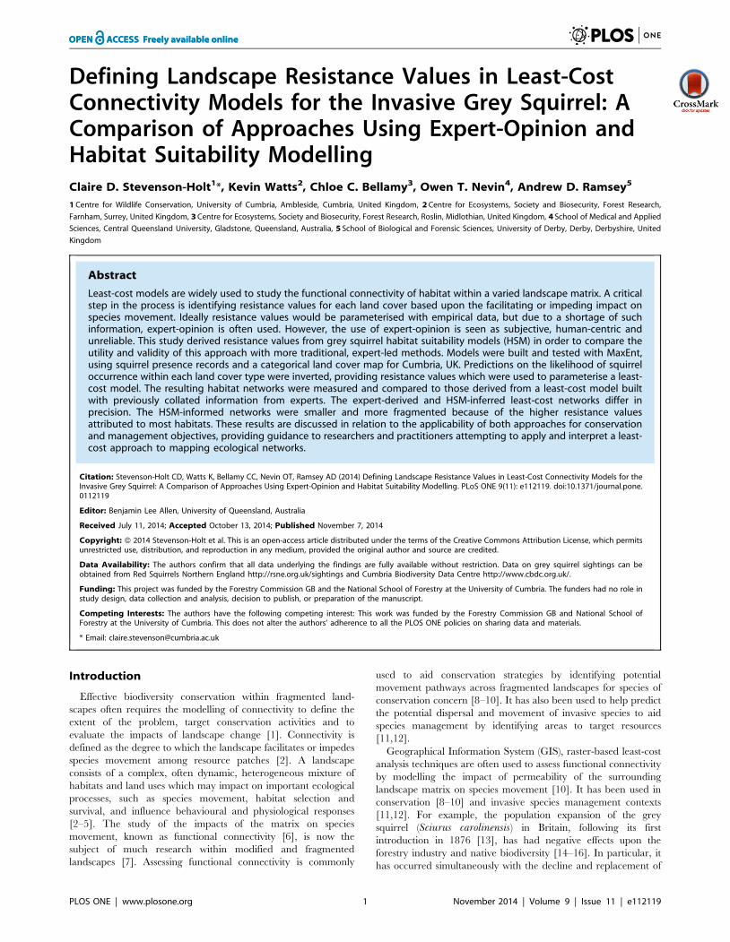
Study siteTo compare expert-derived resistance values against HSM-
informed values, grey squirrel within the county of Cumbria UK
(Figure 1), are used as the study species. Whilst six large
woodlands in Cumbria are designated red squirrel refuge reserves
(Figure 1), the grey squirrel remains throughout the county. A
number of previous studies have used expert-derived least-cost
models to define habitat connectivity for Britain’s native red
squirrels and invasive grey squirrels [33–36], providing expert-
opinion on land cover resistance. In addition, Cumbria has an
extensive collection of grey squirrel distribution records available
with which to create HSM-informed data for comparison.
Cumbria covers an area of 6,768 km2 and has a sparse population
of 490,000 people. The Lake District National Park is located in
the centre of Cumbria and has legislation and planning restrictions
to conserve the landscape. The National Park Authority are
responsible for implementing legislation and planning decisions
aimed at conserving the landscape and its species, which means
that little has changed regarding land use during the time frame
that the species presence data used within this study were recorded
(2000–2009). The topography is varied with the Cumbrian
Mountain range (#978 m a.s.l.) that runs approximately west to
east across the middle of the county. The majority of land at these
higher elevations is used for grazing with little woodland habitat.
However, at lower elevations there are numerous woodlands, and
other semi-natural habitats, scattered within an agricultural matrix
which may provide greater potential for squirrel movement.
Identifying least-cost networksLand cover types from a highly accurate and up to date vector
land cover map (Ordnance Survey Master Map) were reclassified
into 21 broad land cover categories for Cumbria (Table 1). The
map was rasterised at 10 m resolution to ensure accurate
representation of narrow linear features, such as strips of
woodland. All woodland patches were classed as core habitat as
squirrels use these areas for nesting and breeding [37,38]. This
map was then parameterised with five alternative expert-derived
resistance sets from previous studies (Table 1). The resistance
values given in the different studies varied substantially. An
additional set of values was developed by the authors by refining
Stevenson’s [35] scores (referred to as new expert-derived),
following a review of the literature and the ecological underpin-
ning of the values that had been applied previously, as described
below.
Coniferous, mixed and broadleaved woodland were all assigned
the lowest resistance value of 1, as core habitat. Scrub, coppice,
orchard, and garden were given relatively low resistance values
because they often contain tree species and are commonly used by
Defining Landscape Resistance Values in Least-Cost Models
PLOS ONE | www.plosone.org 2 November 2014 | Volume 9 | Issue 11 | e112119
grey squirrels for commuting [11,20]. Path, track, road verge, road
and railway verge may also be used as commuting corridors, [13],
but their use may confer higher mortality risks and therefore they
were assigned a relatively high score. Improved/arable/amenity,
rough grassland and heath were all attributed higher values still, as
squirrel species tend to avoid open habitats [39]. Due to the threat
of railways and the difficulty of moving over marsh, water, urban
areas, buildings, and rocky areas like cliffs, the high scores assigned
in previous studies were maintained.
Least-cost networks were created for each set of resistance
values (Table 1) using the least-cost network process outlined in
Watts et al. [10]. This network tool analysis utilises ArcView 9.1
and the Spatial Analyst extension (ESRI, Redlands, CA). The first
step defined suitable patches of woodland habitat and generated a
cost surface raster from the land cover map, by joining the
resistance values (Table 1) to the 21 land cover classes. Secondly,
the ‘cost-distance’ function in the Spatial Analyst toolbox was used
to create a cost-distance surface between woodland patches. The
resulting accumulated cost raster was then reclassified to a
standardised maximum dispersal distance of 8 km to ensure
comparability between the different resistance sets. The ‘region
group’ function was used to define each discrete network, using an
eight-cell rule so that touching cells, either adjacent and diagonally
opposite, within the minimum distance of any given patch were
considered part of the same network.
Deriving resistance scores from habitat suitabilitymodelling
Records of grey squirrel presence were obtained from Save Our
Squirrels (http://www.saveoursquirrels.org.uk/). These consisted
of 2,281 verified sightings recorded year-round between 2000 and
2009 given by members of the public from both within woodland
habitat (35%) and the wider landscape (65%). The grid references
and type of habitat the sightings were recorded and verified by
Save Our Squirrels. Sightings that were recorded outside of the
grey squirrels known distribution range were also verified by
contacting the recorder. The points outside of core woodland
habitat are believed to relate to landscape use and movement,
rather than indicating suitable foraging, breeding or nesting
resources [37,38]. It is these non-woodland records that are used
to infer the permeability of the landscape matrix using the habitat
suitability modelling software, MaxEnt [40,32]. MaxEnt assigns
each raster cell a Habitat Suitability Index (HSI) based on the
environmental conditions at locations where a species has been
recorded, using the maximum entropy method [41]. There are
three output formats given by the MaxEnt programme: raw,
cumulative and logistic; the most easily intuitive logistic HSI
scores, which indicate the probability of occupancy ranging
between 0–1 and assuming that this is 0.5 at an average site
[40,32], were used in this study.
Both the species records and environmental data were prepared
for modelling with MaxEnt. The squirrel data were filtered to
remove locations recorded at a resolution of .100 m. Of the
remaining 2,008 points, 842 squirrel presences recorded were
Figure 1. Map of red squirrel reserves in Cumbria and neighbouring counties with reference to its location in the UK. * 1. Whinlatter;2. Thirlmere; 3. Greystoke; 4. Whinfell; 5. Garsdale/Mallerstang and 6. Kielder (Cumbria proportion of). Boundary lines were obtained through EDINADigimap Ordnance Survey Service, http://digimap.edina.ac.uk/digimap/home.doi:10.1371/journal.pone.0112119.g001
Defining Landscape Resistance Values in Least-Cost Models
PLOS ONE | www.plosone.org 3 November 2014 | Volume 9 | Issue 11 | e112119
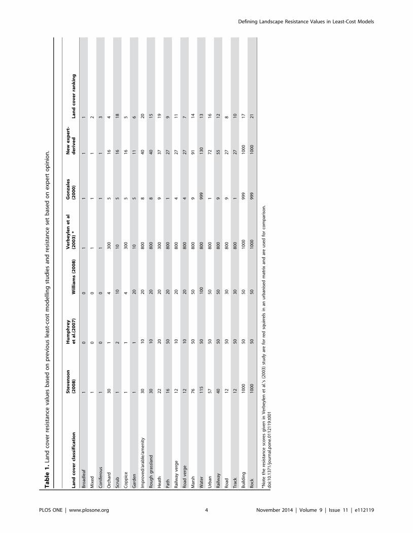
Ta
ble
1.
Lan
dco
ver
resi
stan
ceva
lue
sb
ase
do
np
revi
ou
sle
ast-
cost
mo
de
llin
gst
ud
ies
and
resi
stan
cese
tb
ase
do
ne
xpe
rto
pin
ion
.
La
nd
cov
er
cla
ssif
ica
tio
nS
tev
en
son
(20
08
)H
um
ph
rey
et
al.
(20
07
)W
illi
am
s(2
00
8)
Ve
rbe
yle
ne
ta
l(2
00
3)
*G
on
za
les
(20
00
)N
ew
ex
pe
rt-
de
riv
ed
La
nd
cov
er
ran
kin
g
Bro
adle
af1
00
11
11
Mix
ed
10
01
11
2
Co
nif
ero
us
10
01
11
3
Orc
har
d3
01
43
00
51
64
Scru
b1
21
01
05
16
18
Co
pp
ice
11
43
00
51
65
Gar
de
n1
12
01
05
11
6
Imp
rove
d/a
rab
le/a
me
nit
y3
01
02
08
00
84
02
0
Ro
ug
hg
rass
lan
d3
01
02
08
00
84
01
5
He
ath
22
20
20
30
09
37
19
Pat
h1
65
02
08
00
12
79
Rai
lway
verg
e1
21
02
08
00
42
71
1
Ro
adve
rge
12
10
20
80
04
27
7
Mar
sh7
65
05
08
00
99
11
4
Wat
er
11
55
01
00
80
09
99
13
01
3
Urb
an5
75
05
08
00
17
21
6
Rai
lway
40
50
50
80
09
55
12
Ro
ad1
25
03
08
00
92
78
Tra
ck1
25
03
08
00
12
71
0
Bu
ildin
g1
00
05
05
01
00
09
99
10
00
17
Ro
ck1
00
05
05
01
00
09
99
10
00
21
*No
teth
ere
sist
ance
sco
res
giv
en
inV
erb
eyl
en
et
al.’s
(20
03
)st
ud
yar
efo
rre
dsq
uir
rels
inan
urb
anis
ed
mat
rix
and
are
use
dfo
rco
mp
aris
on
.d
oi:1
0.1
37
1/j
ou
rnal
.po
ne
.01
12
11
9.t
00
1
Defining Landscape Resistance Values in Least-Cost Models
PLOS ONE | www.plosone.org 4 November 2014 | Volume 9 | Issue 11 | e112119
within the matrix. A categorical land cover raster (gridded data
map) was created using the same Ordnance Survey Master Map
data and 21 broad land cover categories as previously described
(Table 1). However, a coarser resolution of 100 m was used to
match the spatial accuracy of the squirrel records. To ensure that
linear habitat features were not under-represented, each land
cover type was rasterised separately at a 10 m resolution and then
aggregated to 100 m using the ‘maximum’ rule. These rasters
were mosaicked using ranks that prioritised the classification of
each 100 m square containing more than one land cover type
(Table 1). All areas of woodland (core habitat), rocks and buildings
(highly impermeable) were removed from the land cover map to
prevent their incorporation in the model. In an effort to account
for sampling bias towards accessible areas, a well-known and
common characteristic of species data collected in an ad-hoc or
non-systematic way [42], all areas over 500 m from a road, track
or path were also removed from the map. This left a total of 665
squirrel records that fell within the remaining areas of the land
cover map which were used to train and test the habitat suitability
model. Each point (located in the south west of the 100 m grid
square) was adjusted by 50 m east and 50 m north to locate each
point in the centre of the grid square. This was to ensure that the
points matched the 100 m raster landscape i.e. were within one
cell, not potentially boarding four.
All models were run in MaxEnt Version 3.3.3k, using primarily
default settings (regularisation multiplier = 1; duplicate occur-
rences removed; maximum number of background points
= 10000, as used in Kramer-Schadt et al. [43]). Five-fold cross
validation was used to calculate mean Area Under Roc Curve
(AUC) and extrinsic omission rates (the average proportion of test
points that fall outside the area predicted to be suitable), following
use of the occupancy threshold rule that maximises the sum of test
sensitivity and specificity (as recommended by Liu et al., [44]).
Residual spatial autocorrelation (rSAC) can inflate measures of
model performance [45–47] therefore Moran’s correlograms were
created (1 – predicted HSI for each species record; [48]) using the
Spatial Analysis in Macroecology software program (SAM; [49]).
Significance of Moran’s I was calculated using a randomisation
test with 9,999 Monte Carlo permutations, correcting for multiple
testing.
The response curves, which showed the mean predicted
probability of a species’ presence (p; 0–1 scale) within each land
cover type, were used to derive the resistance values for each land
cover type. For both the new expert-derived and the HSM-
informed values, woodland was given a value of 1, as permeable
core habitat, and rock and building given values of 1000, as
impermeable land cover types. The remaining land cover type
values were inverted and standardised to the same scale as the new
expert-derived values, (1–130; using 1-(p6130)). These values were
then used to identify least-cost networks using the same approach
as applied to the new expert-derived resistance scores.
Comparing resistance scores and resulting habitatnetworks
An area-minimisation methodology was applied to select for the
smallest network that captures the majority ($90%) of the filtered
distribution point data (n = 842). This methodology, derived
during this study, was based on the principle that when managing
invasive species, areas for control must be defined and defensible
to provide successful management [50]. As the grey squirrel
population continues to expand in the Cumbria study site, it is
important that control efforts are targeted to provide effective
management. By identifying habitat networks management can be
targeted in these specific areas of the landscape. The larger the
habitat networks are the more widespread management would
have to be. Therefore, the resistance set which produced networks
that include a high proportion of distribution points but a small
network area are regarded as the better networks as management
can be targeted in these focused areas. In addition a chi square test
was used to test whether a significant number of distribution points
were within the networks when compared to random points.
The HSM-informed resistance scores and the resulting networks
were compared to those created with the new expert-derived set
selected by the area-minimisation criteria. A Wilcoxon signed
ranks test was used to assess the relative difference between scores.
The habitat networks produced were also measured and compared
visually and using the distribution points. Distribution points that
were within the new expert-derived networks but not within the
HSM-informed networks were identified along with the land cover
type they were in and vice versa.
Results
Habitat Suitability Model performanceThe results from five-fold cross-validation test showed that the
models performed well (Training sample size = 532; Test sample
size = 133; Training AUC = 0.8060.001; Test
AUC = 0.7860.04; Test gain = 0.7060.19; Extrinsic omission
rate = 0.23, P,0.001), indicating that land cover type provides
useful information on the likelihood of grey squirrel presence. No
significant residual spatial autocorrelation was found at any
distance lag. Moran’s I values were ,0.05 and statistically
insignificant at each distance lag, indicating that the residuals
were not spatially autocorrelated.
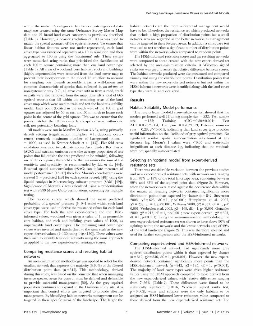
Selecting an ‘optimal model’ from expert-derivedresistance sets
There was considerable variation between the previous studies
and new expert-derived resistance sets, with network area ranging
from 78% to 15% of the total landscape area, containing between
99% and 32% of the squirrel point data (Figure 2). However,
when the networks were tested against the occurrence data within
the matrix all resulting networks contained significantly more
distribution points than expected by chance (n = 842, Stevenson
2008, x2 = 623, df. = 1, p,0.001; Humphreys et al. 2007,
x2 = 238, df. = 1, p,0.001; Williams 2008, x2 = 357, df. = 1, p,
0.001; Verbeylen et al. 2003, x2 = 169, df. = 1, p,0.001; Gonzales
2000, x2 = 213, df. = 1, p,0.001; new expert-derived, x2 = 623,
df. = 1, p,0.001). Using the area-minimisation methodology, the
new expert-derived resistance set was shown to have above 90% of
sightings within the networks and the lowest networks area of 49%
of the total landscape (Figure 2). This was therefore selected and
used for further comparison with the HSM-informed networks.
Comparing expert-derived and HSM-informed networksThe HSM-informed network had significantly more grey
squirrel distribution points within it than expected by chance
(n = 842, x2 = 836, df. = 1, p,0.001). However, the new expert-
derived network contained significantly more points than the
HSM-informed network (n = 842, x2 = 185, df. = 1, p,0.001).
The majority of land cover types were given higher resistance
values using the HSM approach compared to those derived from
the new expert-derived values, with relative differences ranging
from 7–86% (Table 2). These differences were found to be
statistically significant (n = 16, Wilcoxon signed ranks test,
p = 0.002); water and coppice were the only habitats to be
assigned an HSM-informed lower resistance value compared to
those derived from the new expert-derived resistance set. The
Defining Landscape Resistance Values in Least-Cost Models
PLOS ONE | www.plosone.org 5 November 2014 | Volume 9 | Issue 11 | e112119
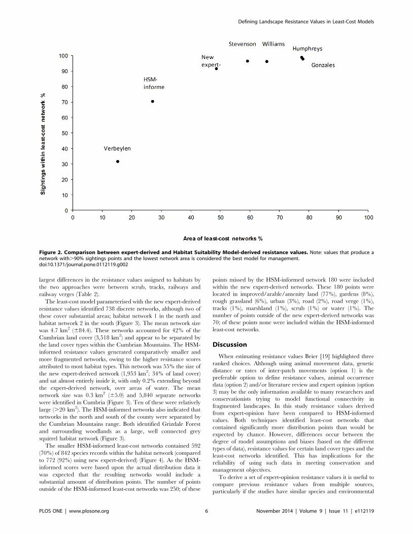
largest differences in the resistance values assigned to habitats by
the two approaches were between scrub, tracks, railways and
railway verges (Table 2).
The least-cost model parameterised with the new expert-derived
resistance values identified 738 discrete networks, although two of
these cover substantial areas; habitat network 1 in the north and
habitat network 2 in the south (Figure 3). The mean network size
was 4.7 km2 (684.4). These networks accounted for 42% of the
Cumbrian land cover (3,518 km2) and appear to be separated by
the land cover types within the Cumbrian Mountains. The HSM-
informed resistance values generated comparatively smaller and
more fragmented networks, owing to the higher resistance scores
attributed to most habitat types. This network was 55% the size of
the new expert-derived network (1,953 km2; 34% of land cover)
and sat almost entirely inside it, with only 0.2% extending beyond
the expert-derived network, over areas of water. The mean
network size was 0.3 km2 (65.0) and 5,840 separate networks
were identified in Cumbria (Figure 3). Ten of these were relatively
large (.20 km2). The HSM-informed networks also indicated that
networks in the north and south of the county were separated by
the Cumbrian Mountains range. Both identified Grizdale Forest
and surrounding woodlands as a large, well connected grey
squirrel habitat network (Figure 3).
The smaller HSM-informed least-cost networks contained 592
(70%) of 842 species records within the habitat network (compared
to 772 (92%) using new expert-derived) (Figure 4). As the HSM-
informed scores were based upon the actual distribution data it
was expected that the resulting networks would include a
substantial amount of distribution points. The number of points
outside of the HSM-informed least-cost networks was 250; of these
points missed by the HSM-informed network 180 were included
within the new expert-derived networks. These 180 points were
located in improved/arable/amenity land (77%), gardens (8%),
rough grassland (6%), urban (3%), road (2%), road verge (1%),
tracks (1%), marshland (1%), scrub (1%) or water (1%). The
number of points outside of the new expert-derived networks was
70; of these points none were included within the HSM-informed
least-cost networks.
Discussion
When estimating resistance values Beier [19] highlighted three
ranked choices. Although using animal movement data, genetic
distance or rates of inter-patch movements (option 1) is the
preferable option to define resistance values, animal occurrence
data (option 2) and/or literature review and expert opinion (option
3) may be the only information available to many researchers and
conservationists trying to model functional connectivity in
fragmented landscapes. In this study resistance values derived
from expert-opinion have been compared to HSM-informed
values. Both techniques identified least-cost networks that
contained significantly more distribution points than would be
expected by chance. However, differences occur between the
degree of model assumptions and biases (based on the different
types of data), resistance values for certain land cover types and the
least-cost networks identified. This has implications for the
reliability of using such data in meeting conservation and
management objectives.
To derive a set of expert-opinion resistance values it is useful to
compare previous resistance values from multiple sources,
particularly if the studies have similar species and environmental
Figure 2. Comparison between expert-derived and Habitat Suitability Model-derived resistance values. Note: values that produce anetwork with.90% sightings points and the lowest network area is considered the best model for management.doi:10.1371/journal.pone.0112119.g002
Defining Landscape Resistance Values in Least-Cost Models
PLOS ONE | www.plosone.org 6 November 2014 | Volume 9 | Issue 11 | e112119
conditions. The resistance values given in previous studies were
highly variable, resulting in varied least-cost habitat network areas
and number of distribution points within networks. Although the
land cover resistance values given in these studies were for red or
grey squirrels, the studies took place in different countries with
different regional environmental conditions and large scale and
inevitable differences in landscape composition and structure. This
may account for the differences in values given and resulting
networks. Verbeylen et al [3] in particular was focused on red
squirrels and based in an urban area which is very different to the
largely-rural and sparsely populated Cumbria. However by
assessing the range of different resistance values given in these
studies and additional literature on land cover use, the new expert-
derived resistance set was created. The area-minimisation method
suggests that these values appear to be the best set for management
purposes in this area, capturing a high percentage of distribution
points within the smallest network area.
The resistance values for the new expert-derived and HSM-
informed least-cost models in this study were significantly different
from one another. The HSM-informed model provided higher
resistance values for most land cover types. The validity of HSM-
informed least-cost models may be limited as the probability of
occurrence in a particular land cover type does not always equate
to the resistance of that land cover type during species movement
[19]. In using distribution/occurrence data, certain land cover
types may be undervalued when in reality they are used by the
species. Conversely there will be land cover types that are
overvalued. A key assumption of presence only modelling is that
the data has come from random sampling or is representative of
the whole landscape [51]. It is questionable whether the degree of
bias in presence data can be truly known [51]. Squirrels are well
known to use scrub habitat and will use this and linear features to
aid dispersal [13,52–54], yet scrub and railway verge (a linear
feature) were given high HSM-informed resistance values due to a
low number of distribution points. Of the distribution points
missed by the HSM-informed networks but included within the
new expert-derived networks, 77% were within improved/arable/
amenity land cover type. This suggests that the inverted HSM
values for this land cover may be too high, and squirrels may be
able to cross these hostile areas quickly and undetected. The
dispersal distance used for both expert-derived model and the
HSM-informed model were set at 8 km. Therefore, it is the higher
resistance values given to certain land cover types using the
inverted-HSM that led to the identification of smaller and more
fragmented networks.
The HSM-informed networks were 45% smaller than the
expert-derived networks and were spatially nested inside these
networks. The smaller mean size of HSM-informed networks
suggests that grey squirrel occurs in a highly fragmented and
functionally unconnected landscape. Both models highlight the
land cover types of the Cumbrian Mountains as a barrier to
movement; the combination of relatively high elevation and
intense grazing result in a lack of woodland in the area. Although,
some individuals may attempt to cross the barrier, the lack of
available habitat will impede dispersal subjecting individuals to
high levels of predation and starvation. There are no recorded
introductions of the grey squirrel into Cumbria [55,56] and
therefore these animals have been able to spread to their present
Table 2. Average probability of grey squirrel presence according to land cover type.
Habitat typeHSMp score
HSM-resistancescore
New expert-derivedresistance score
Difference between HSM and Expert-derivedresistance scores
Scrub 0.10 117 16 0.86
Track 0.16 109 27 0.75
Railway 0.17 108 27 0.75
Railway verge 0.17 108 27 0.75
Path 0.34 86 27 0.69
Heath 0.17 108 37 0.66
Garden 0.73 32 11 0.66
Road 0.41 77 27 0.65
Improved/arable/amenity
0.13 113 40 0.65
Rough grassland 0.13 113 40 0.65
Road verge 0.43 74 27 0.64
Orchard 0.77 30 16 0.47
Urban 0.29 92 72 0.22
Marsh 0.17 108 91 0.16
Broadleaf N/A 1 1 0.00
Coniferous N/A 1 1 0.00
Mixed N/A 1 1 0.00
Building N/A 1000 1000 0.00
Rock N/A 1000 1000 0.00
Coppice 0.86 15 16 20.07
Water 0.18 107 130 20.21
p = mean predicted probability of presence according to habitat type.doi:10.1371/journal.pone.0112119.t002
Defining Landscape Resistance Values in Least-Cost Models
PLOS ONE | www.plosone.org 7 November 2014 | Volume 9 | Issue 11 | e112119
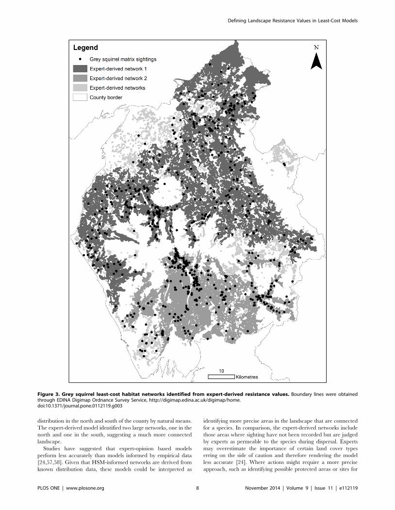
distribution in the north and south of the county by natural means.
The expert-derived model identified two large networks, one in the
north and one in the south, suggesting a much more connected
landscape.
Studies have suggested that expert-opinion based models
perform less accurately than models informed by empirical data
[24,57,58]. Given that HSM-informed networks are derived from
known distribution data, these models could be interpreted as
identifying more precise areas in the landscape that are connected
for a species. In comparison, the expert-derived networks include
those areas where sighting have not been recorded but are judged
by experts as permeable to the species during dispersal. Experts
may overestimate the importance of certain land cover types
erring on the side of caution and therefore rendering the model
less accurate [24]. Where actions might require a more precise
approach, such as identifying possible protected areas or sites for
Figure 3. Grey squirrel least-cost habitat networks identified from expert-derived resistance values. Boundary lines were obtainedthrough EDINA Digimap Ordnance Survey Service, http://digimap.edina.ac.uk/digimap/home.doi:10.1371/journal.pone.0112119.g003
Defining Landscape Resistance Values in Least-Cost Models
PLOS ONE | www.plosone.org 8 November 2014 | Volume 9 | Issue 11 | e112119
an efficient and intensive control program, a HSM modelling
approach would be appropriate. However, when assessing invasive
species it is not just the most likely areas that a species will disperse
to, but the entire possible range that needs identified. In an
invasive species context, it may be more appropriate to apply a
conservative less precise model, such as the expert-derived model,
to enable all possible areas of dispersal to be included within the
network.
In the case of invasive species the assessment of potential
movement and impact is needed as soon as possible to aid
management planning. This method is not dependent upon
extensive species distribution data and can therefore be produced
relatively quickly. Clevenger et al. [24] found that expert only
derived resistance values had a weaker correlation with empirical-
derived values than literature-derived values. Systematically
collecting expert opinion, as promoted by Eycott et al [59], in
Figure 4. Highly fragmented grey squirrel least-cost habitat networks identified with Habitat Suitability Model-derived resistancevalues. Boundary lines were obtained through EDINA Digimap Ordnance Survey Service, http://digimap.edina.ac.uk/digimap/home.doi:10.1371/journal.pone.0112119.g004
Defining Landscape Resistance Values in Least-Cost Models
PLOS ONE | www.plosone.org 9 November 2014 | Volume 9 | Issue 11 | e112119
combination with published data on land cover usage will enable
resistance values to be assigned in the initial stages to give an
indication of species movements whilst other empirical data is
collected where possible. Adriensen et al [18] suggested that once a
‘starter kit’ of resistance values has been identified, sensitivity
studies can be initiated and multiple alternative resistance sets can
be tested [60]. Once species distribution data is collected, HSM-
informed least-cost networks can be identified and used to aid the
selection of most likely used sites to focus monitoring or
eradication programs. It should not be assumed that using
distribution data (option 2 in Beier et al. [19]) to identify
resistance values is better or worse than using well developed
expert-opinion (option 3 in Beier et al. [19]) as the choice of which
method to use may depend upon the aims and objectives of the
user and the appropriate precision of the approach.
This paper describes the first step towards developing least-cost
habitat networks using ad hoc species records and a simple, land
cover-based habitat suitability model. It is acknowledged, howev-
er, that species respond to their surrounding environment over a
range of spatial scales and that both local and landscape features
will affect both the suitability of the core habitat and the
permeability of the surrounding matrix [5,61]. More complex
models incorporating multiscale information on the terrain, built
environment, and the composition, structure and arrangement of
habitat patches are likely to provide more accurate and useful
models [45], providing predictions at each location, rather than
assuming consistent levels of permeability for a particular land
cover type. This spatially explicit technique would enable
landscape level decision making, improving our ability to identify
important networks of habitat and enabling a targeted and
informed approach to both conservation and infrastructural
development.
ConclusionEven though approaches to gather expert opinion are becoming
more systematic and robust, it should not be seen as a blanket
substitute for empirical data. Empirical data will continue to be
important for studies on single species, where there is considerable
uncertainty or where there is significant investment in time and
money on conservation activities. Conservation planners must be
aware of the subjectivity and pitfalls of the different types of data
used in least-cost models, without any further validation or
sensitivity testing of model values. If expert opinion is the only
option available it should be used as a first step by systematically
combining multiple expert opinions and published data, but with
the knowledge that further assessment of resistance values through
sensitivity analysis and empirical data will be needed. Where
distribution data is already available, the type of data collection
and the subjective translation issues of over and under valuing land
cover types must be assessed with expert knowledge or empirical
data and explicitly stated in methodologies [51,62].
This study successfully compared expert-derived and HSM-
informed resistance values used in least-cost modelling. Although
the results of the models differed, both identified equally useful
least-cost networks. For the grey squirrel in Cumbria, both expert-
derived and HSM-informed networks have shown that there is a
separation between north and south of Cumbria due to the land
cover types and lack of habitat of the Cumbrian Mountain range.
The expert-derived networks indicate a conservative less precise
least-cost network that indicates the potential dispersal range of the
grey squirrel and suggests that there may be multiple infiltration
routes into the county from the north and south. This conservative
expert-derived approach is useful when dealing with invasive or
generalist species to identify the potential extend of spread. When
assessing endangered or specialist species, or areas that are highly
likely to contain target species, the HSM-informed network
provides smaller precise networks. These precise networks should
be used to inform targeted conservation to increase connectivity
for species of conservation concern, or to inform targeted
management to prevent the incursion of invasive species. The
variable but acceptable precision of both expert-derived and
HSM-informed least-cost networks highlights the need to consider
data reliability and environmental context when deciding on the
most appropriate management of invasive species.
Acknowledgments
The Authors would like to thank Dr Sallie Bailey for advice and comments,
Phillip Handley for GIS advice and Simon O’Hare for sightings data.
Country and county outlines in Figures 1, 3 and 4 and OSMM data were
obtained through EDINA Digimap Ordnance Survey Service, http://
digimap.edina.ac.uk/digimap/home.
Author Contributions
Conceived and designed the experiments: CDSH KW OTN ADR.
Performed the experiments: CDSH KW CB. Analyzed the data: CDSH
KW CB. Contributed reagents/materials/analysis tools: CDSH KW CB
OTN ADR. Wrote the paper: CDSH KW CB OTN ADR.
References
1. Worboys G, Francis WL, Lockwood M (2009) Connectivity conservation
management: A global guide (with particular reference to mountain connectivityconservation). London: Earthscan/James & James.
2. Taylor PD, Fahrig L, Henein K, Merriam G (1993) Connectivity is a vitalelement of landscape structure. Oikos 68: 571–573.
3. Verbeylen G, De Bruyn L, Adriaensen F, Matthysen E (2003) Does matrixresistance influence red squirrel (Sciurus vulgaris L. 1978) distribution in an
urban landscape? Landscape Ecology 18: 791–805.
4. Spear SF, Balkenhol N, Fortin MJ, McRae BH, Scribner K (2010) Use of
resistance surfaces for landscape genetic studies: Considerations for parameter-ization and analysis. Mol Ecol 19: 3576–3591.
5. Ricketts TH (2001) The matrix matters: Effective isolation in fragmentedlandscapes. The American Naturalist 158: 87–99.
6. Tischendorf L, Fahrig L (2000) On the usage and measurement of landscapeconnectivity. Oikos 90: 7–19.
7. Crooks KR (2006) Connectivity conservation. Cambridge: Cambridge Univ Pr.
8. Ferreras P (2001) Landscape structure and asymmetrical inter-patch connectivity
in a metapopulation of the endangered Iberian lynx. Biol Conserv 100: 125–136.
9. Epps CW, Wehausen JD, Bleich VC, Torres SG, Brashares JS (2007)
Optimizing dispersal and corridor models using landscape genetics. J Appl Ecol
44: 714–724.
10. Watts K, Eycott AE, Handley P, Ray D, Humphrey JW, et al. (2010) Targeting
and evaluating biodiversity conservation action within fragmented landscapes:
An approach based on generic focal species and least-cost networks. Landscape
Ecology 25: 1305–1318.
11. Stevenson CD, Ferryman M, Nevin OT, Ramsey AD, Bailey S, et al. (2013)
Using GPS telemetry to validate least-cost modeling of gray squirrel (Sciuruscarolinensis) movement within a fragmented landscape. Ecology and Evolution
3: 2350–2361.
12. Gonzales EK, Gergel SE (2007) Testing assumptions of cost surface analysis- a
tool for invasive species management. Landscape Ecology 22: 1155–1168.
13. Middleton AD (1930) The ecology of the American grey squirrel (Sciuruscarolinensis gmelin) in the British isles. J Zool, Lond. 100: 809–843.
14. Gurnell J, Wauters LA, Lurz PWW, Tosi G (2004) Alien species and interspecific
competition: Effects of introduced eastern grey squirrels on red squirrel
population dynamics. J Anim Ecol 73: 26–35.
15. Gurnell J, Mayle B (2003) Ecological impacts of the alien grey squirrel (Sciuruscarolinensis) in Britain. In Bowen CP, editor. MammAliens – A one day
conference on the problems caused by non- native British mammals. London:
Peoples Trust for Endangered Species/Mammals Trust UK. pp.40–45.
16. Kenward RE (1983) The causes of damage by red and grey squirrels. Mamm
Rev 13: 159–166.
17. Sawyer SC, Epps CW, Brashares JS (2011) Placing linkages among fragmented
habitats: Do least-cost models reflect how animals use landscapes? J Appl Ecol
48: 668–678.
Defining Landscape Resistance Values in Least-Cost Models
PLOS ONE | www.plosone.org 10 November 2014 | Volume 9 | Issue 11 | e112119
18. Adriaensen F, Chardon JP, De Blust G, Swinnen E, Villalba S, et al. (2003) The
application of ‘least-cost’ modelling as a functional landscape model. Landscapeand Urban Planning 64: 233–247.
19. Beier P, Majka DR, Spencer WD (2008) Forks in the road: Choices in
procedures for designing wildland linkages. Conserv Biol 22: 836–851.20. Driezen K, Adriaensen F, Rondinini C, Doncaster CP, Matthysen E (2007)
Evaluating least-cost model predictions with empirical dispersal data: A case-study using radio tracking data of hedgehogs (Erinaceus europaeus). Ecological
Modelling 209: 314–322.
21. Stevens VM, Polus E, Wesselingh RA, Schtickzelle N, Baguette M (2005)Quantifying functional connectivity: Experimental evidence for patch-specific
resistance in the natterjack toad (Bufo calamita). Landscape Ecol 19: 829–842.22. Eycott AE, Stewart GB, Buyung-Ali LM, Bowler DE, Watts K, et al. (2012) A
meta-analysis on the impact of different matrix structures on species movementrates. Landscape Ecol 27: 1263–1278.
23. Zeller KA, McGarigal K, Whiteley AR (2012) Estimating landscape resistance to
movement: A review. Landscape Ecol 27: 777–797.24. Clevenger AP, Wierzchowski J, Chruszcz B, Gunson K (2002) GIS-generated,
expert-based models for identifying wildlife habitat linkages and planningmitigation passages. Conserv Biol 16: 503–514.
25. Chardon JP, Adriaensen F, Matthysen E (2003) Incorporating landscape
elements into a connectivity measure: A case study for the speckled woodbutterfly (Pararge aegeris L.). Landscape Ecology 18: 561–573.
26. Wang Y, Yang K, Bridgman CL, Lin L (2008) Habitat suitability modelling tocorrelate gene flow with landscape connectivity. Landscape Ecol 23: 989–1000.
27. Richards-Zawacki CL (2009) Effects of slope and riparian habitat connectivityon gene flow in an endangered Panamanian frog, Atelopus varius. Divers Distrib
15: 796–806.
28. Decout S, Manel S, Miaud C, Luque S (2010) Connectivity loss in humandominated landscape: Operational tools for the identification of suitable habitat
patches and corridors on amphibian’s population. Landscape InternationalConference IUFRO, Portugal.
29. Wang IJ, Summers K (2010) Genetic structure is correlated with phenotypic
divergence rather than geographic isolation in the highly polymorphicstrawberry poison-dart frog. Mol Ecol 19: 447–458.
30. Decout S, Manel S, Miaud C, Luque S (2012) Integrative approach forlandscape-based graph connectivity analysis: A case study with the common frog
(Rana temporaria) in human-dominated landscapes. Landscape Ecol 27: 267–279.
31. Howard A, Bernardes S (2012) A maximum entropy and least cost path model of
bearded capuchin monkey movement in Northeastern brazil. Intergraph.Available: https://intergraphgovsolutions.com/assets/white-paper/A_
Maximum_Entropy-2_Imagery.sflb.pdf Accessed 2013.32. Phillips SJ, Anderson RP, Schapire RE (2006) Maximum entropy modeling of
species geographic distributions. Ecol Model 190: 231–259.
33. Gonzales EK (2000) Distinguishing between modes of dispersal by introducedeastern grey squirrels (Sciurus carolinensis). MSc Thesis, University of Guelph.
34. Humphrey J, Smith M, Shepherd N, Handley P (2007) Developing lowlandhabitat networks in Scotland: Phase 2. Edinburgh: Forestry Commission.
35. Stevenson CD (2008) Modelling red squirrel population viability under a rangeof landscape scenarios in fragmented woodland ecosystems on the Solway plain,
Cumbria. London: People’s Trust for Endangered Species. Available http://
insight.cumbria.ac.uk. Accessed 2013.36. Williams S (2008) Red squirrel strongholds consultation. Edinburgh: Forestry
Commission.37. Lowe VPW (1993) The spread of the grey squirrel (Sciurus carolinensis) into
Cumbria since 1960 and its present distribution. J Zool, Lond 231: 663–667.
38. Skelcher G (1997) The ecological replacement of red by grey squirrels. In:Gurnell J, Lurz P, editors. The conservation of red squirrels, Sciurus vulgaris L.
London: People’s Trust for Endangered Species. pp.67–78.
39. Nixon CM, McClain MW, Donohoe RW (1980) Effects of clear-cutting on grey
squirrels. Journal of Wildlife Management 44: 403–412.
40. Phillips SJ, Dudik M (2008) Modeling of species distributions with maxent: New
extensions and a comprehensive evaluation. Ecography 31: 161–175.
41. Phillips SJ, Dudı́k M, Elith J, Graham CH, Lehmann A, et al. (2009) Sample
selection bias and presence-only distribution models: Implications for back-
ground and pseudo-absence data. Ecol Appl 19: 181–197.
42. Warton DI, Renner IW, Ramp D (2013) Model-based control of observer bias
for the analysis of presence-only data in ecology. Plos One 8: e79168.
43. Schadt S, Knauer F, Kaczensky P, Revilla E, Wiegand T, et al. (2002) Rule-
based assessment of suitable habitat and patch connectivity for the Eurasian
lynx. Ecol Appl 12: 1469–1483.
44. Liu C, White M, Newell G (2013) Selecting thresholds for the prediction of
species occurrence with presence-only data. J Biogeogr 40: 778–789.
45. Bellamy C, Scott C, Altringham J (2013) Multiscale, presence-only habitat
suitability models: Fine-resolution maps for eight bat species. J Appl Ecol 50:
892–901.
46. Merckx B, Steyaert M, Vanreusel A, Vincx M, Vanaverbeke J (2011) Null
models reveal preferential sampling, spatial autocorrelation and overfitting in
habitat suitability modelling. Ecol Model 222: 588–597.
47. Veloz SD (2009) Spatially autocorrelated sampling falsely inflates measures of
accuracy for presence-only niche models. J Biogeogr 36: 2290–2299.
48. De Marco P, Diniz-Filho JA, Bini LM (2008) Spatial analysis improves species
distribution modelling during range expansion. Biol Lett 4: 577–580.
49. Rangel TF, Diniz-Filho JAF, Bini LM (2010) SAM: A comprehensive
application for spatial analysis in macroecology. Ecography 33: 46–50.
50. Zalewski A, Piertney SB, Zalewska H, Lambin X (2009) Landscape barriers
reduce gene flow in an invasive carnivore: Geographical and local genetic
structure of American mink in Scotland. Mol Ecol 18: 1601–1615.
51. Yackulic CB, Chandler R, Zipkin EF, Royle JA, Nichols JD, et al. (2013)
Presence-only modelling using MaxEnt: When can we trust the inferences?
Methods in Ecology and Evolution 4: 236–243.
52. Taylor KD, Shorten M, Lloyd HG, Courtier FA (1971) Movements of the grey
squirrel as revealed by trapping. J Appl Ecol 8: 123–146.
53. Fitzgibbon CD (1993) The distribution of grey squirrel dreys in farm woodland:
The influence of wood area, isolation and management. J Appl Ecol 30: 736–
742.
54. Wauters LA, Gurnell J, Currado I, Mazzoglio P (1997) Grey squirrel Sciuruscarolinensis management in Italy - squirrel distribution in a highly fragmented
landscape. Wildlife Biology 3: 117–123.
55. Shorten M (1954) Squirrels. London: Collins.
56. Shorten M (1957) Squirrels in England, Wales and Scotland, 1955. J Animal
Ecol 26: 287–294.
57. Pearce J, Cherry K, Whish G (2001) Incorporating expert opinion and fine-scale
vegetation mapping into statistical models of faunal distribution. J Appl Ecol 38:
412–424.
58. Seoane J, Bustamante J, Diaz-Delgado R (2005) Effect of expert opinion on the
predictive ability of environmental models of bird distribution. Conserv Biol 19:
512–522.
59. Eycott AE, Marzano M, Watts K (2011) Filling evidence gaps with expert
opinion: The use of Delphi analysis in least-cost modelling of functional
connectivity. Landscape Urban Plann 103: 400–409.
60. Rayfield B, Fortin MJ, Fall A (2010) The sensitivity of least-cost habitat graphs to
relative cost surface values. Landscape Ecol 25: 519–532.
61. Wiens JA (1989) Spatial scaling in ecology. Funct Ecol 3: 385–397.
62. Beier P, Majka DR, Newell SL (2009) Uncertainty analysis of least-cost modeling
for designing wildlife linkages. Ecological Applications 19: 2067–2077.
Defining Landscape Resistance Values in Least-Cost Models
PLOS ONE | www.plosone.org 11 November 2014 | Volume 9 | Issue 11 | e112119