Incompressible Polar Active Matter: Defects,Coarsening and Turbulence
A thesis
Submitted to theTata Institute of Fundamental Research, Mumbai
for the degree ofDoctorate of Philosophy in Physics
by
Navdeep Rana
Tata Institute of Fundamental Research
Tifr Center for Interdisciplinary SciencesHyderabad, India
September, 2021

To the open-source community
Publications relevant to the thesis
1. Navdeep Rana, Pushpita Ghosh, and Prasad Perlekar, “Spreading of nonmotile bacteria
on a hard agar plate: Comparison between agent-based and stochastic simulations”.
In Physical Review E 96, 052403 (2017).
2. Navdeep Rana and Prasad Perlekar, “Coarsening in the 2D incompressible Toner-Tu
equation: Signatures of turbulence”. In Physical Review E 102, 032617 (2020).
3. Navdeep Rana and Prasad Perlekar, “Phase-ordering, topological defects, and turbu-
lence in the 3D incompressible Toner-Tu equation”. In arxiv:2106.03383
4. Navdeep Rana, Rayan Chatterjee, Sriram Ramaswamy, and Prasad Perlekar, “Dense sus-
pensions of polar active particles: Stability and Turbulence”. Manuscript under
preparation.
5. Navdeep Rana, Gaurav Garg, Prathu B. Tiwari, Sayak Bhowmick and Prasad Perlekar,
“Turbulence on a DGX Station : a GPGPU pseudo-spectral solver”. Manuscript
under preparation.
Other publications
1. Rayan Chatterjee, Navdeep Rana, R. Aditi Simha, Prasad Perlekar and Sriram Ramaswamy,
“Inertia drives a flocking phase transition in viscous active fluids”. In arxiv:1907.03492.
To appear in Physical Review X.
| iii

Acknowledgments
I am grateful for all the support my thesis advisor Prasad Perlekar has provided me through-
out my doctoral research. I thank him for being patient with me and help me understand
things better. I would like to extend my gratitude towards my collaborators Akshi Gupta,
Debjani Paul, Gaurav Garg, Pushpita Ghosh, Purnima Jain, Rayan Chatterjee, Sriram
Ramaswamy and Vikash Pandey. I enjoyed working with them a lot.
I thank my thesis committee members Smarajit Karmakar and Surajit Sengupta for
their helpful advice throughout the years. I have learnt a lot (dare I say) from the courses
taught by Mustansir Barma, N.D. Hari Dass, Prasad Perlekar, Rama Govindarajan, Sagar
Chakraborty, Shubha Tiwari, Smarajit Karmakar, Sriram Ramaswamy, Subodh Shenoy and
Tamal Das. I am indebted to Gaurav Garg for teaching me Cuda programming.
I thank my teachers Ashwani Kumar, Balraj Bandral, Kanchan Bala, Kanta Sharma,
Madhu Sharma, Neena Awasthi, Sudhir Awasthi, S. K. Soni, V. K. Vats and Yuvraj Sharma
for their constant support in my school and college years.
Most of the work in this thesis would not have been possible without the efforts of open-
source developers, who have spent countless hours creating excellent quality software that
I used daily. To mention a few, I thank the developers of Vim, Neovim, Linux, Cinnamon,
Paraview, Gnuplot, Numpy, Scipy and Matplotlib.
I will fondly remember the time I have spent with the theory group in TIFR Hyderabad
discussing physics and myriad other things. A special thanks to Kabir for all the coffee
table discussions.
I want to express my gratitude to TIFR Hyderabad and the Department of Atomic
Energy for funding support. I thank TIFR Hyderabad HPC facility for computational
resources and Kalyan, Suman and Srinidhi for technical support.
PhD life would not have been so good without my friends in Hyderabad and home.
Anusheela, Arpita, Debankur, Delta, Jose, Kallol, Mukul, Nikhita, Pankaj, Pappu, Raju,
Sharada, Sumit, Tapas, Vikash and Vishnu made my times memorable in TIFR Hyderabad.
| v

Friends at home, Abhimanyu, Abhishek, Aruna, Ashish, Bharti, Jaswinder, Manav, Nitin,
Priyanka, Rakesh and Vivek, have always supported me. A special thanks to the members
of TIFR-H sports groups and The GrimCamRiPper for all the games and plays. I will
surely miss putting up lively performances with Plain Blue Jeans.
Finally, this would not have been possible without the constant support from my family.
I thank them for always looking out for me and for their constant care and love.
vi |
Contents
1 Introduction 1
1.1 Active Matter . . . . . . . . . . . . . . . . . . . . . . . . . . . . . . . . . . . 1
1.2 Hydrodynamic formalism: Polar order parameter . . . . . . . . . . . . . . . 4
1.3 Hydrodynamic formalism: Momentum conservation . . . . . . . . . . . . . . 5
1.3.1 Dry active matter . . . . . . . . . . . . . . . . . . . . . . . . . . . . 5
1.3.2 Wet active matter . . . . . . . . . . . . . . . . . . . . . . . . . . . . 7
1.4 Hydrodynamic formalism: Number conservation . . . . . . . . . . . . . . . . 10
1.4.1 Malthusian active matter . . . . . . . . . . . . . . . . . . . . . . . . 10
1.4.2 Incompressible active matter . . . . . . . . . . . . . . . . . . . . . . 10
1.5 Topological defects in polar active systems . . . . . . . . . . . . . . . . . . . 12
1.5.1 Incompressible topological defects . . . . . . . . . . . . . . . . . . . . 13
1.6 Activity in bacteria colonies growing on hard substrates . . . . . . . . . . . . 15
1.7 A guide to this thesis . . . . . . . . . . . . . . . . . . . . . . . . . . . . . . . 16
2 Coarsening in the two-dimensional incompressible Toner-Tu equation 19
2.1 Introduction . . . . . . . . . . . . . . . . . . . . . . . . . . . . . . . . . . . . 19
2.2 Model . . . . . . . . . . . . . . . . . . . . . . . . . . . . . . . . . . . . . . . 20
2.3 Dimensionless ITT equation . . . . . . . . . . . . . . . . . . . . . . . . . . . 21
2.4 Vortex solution for the ITT equation . . . . . . . . . . . . . . . . . . . . . . 22
2.5 Coarsening dynamics of the ITT equation . . . . . . . . . . . . . . . . . . . 24
2.6 Vortex merger dynamics . . . . . . . . . . . . . . . . . . . . . . . . . . . . . 25
2.7 Energy dissipation rate and energy spectrum . . . . . . . . . . . . . . . . . . 27
2.7.1 Energy dissipation rate . . . . . . . . . . . . . . . . . . . . . . . . . . 27
2.7.2 Energy dissipation rate and the coarsening length scale . . . . . . . . 28
2.7.3 Energy spectrum and enstrophy budget . . . . . . . . . . . . . . . . 31
2.8 Structure functions . . . . . . . . . . . . . . . . . . . . . . . . . . . . . . . . 34
| vii
2.9 Effect of noise on the coarsening dynamics . . . . . . . . . . . . . . . . . . . 35
2.10 Coarsening in ITT versus bacterial turbulence . . . . . . . . . . . . . . . . . 36
2.11 Pseudo-spectral algorithm for the 2D ITT equation . . . . . . . . . . . . . . 36
2.12 Comparison with Nek5000 . . . . . . . . . . . . . . . . . . . . . . . . . . . . 39
2.13 Conclusions . . . . . . . . . . . . . . . . . . . . . . . . . . . . . . . . . . . . 39
3 Phase ordering, defects, and turbulence in the 3D incompressible Toner-Tu
equation 41
3.1 Introduction . . . . . . . . . . . . . . . . . . . . . . . . . . . . . . . . . . . . 41
3.2 Direct numerical simulations . . . . . . . . . . . . . . . . . . . . . . . . . . 43
3.3 Results . . . . . . . . . . . . . . . . . . . . . . . . . . . . . . . . . . . . . . 44
3.3.1 Average velocity . . . . . . . . . . . . . . . . . . . . . . . . . . . . . 44
3.3.2 Excess free energy surfaces and topological defects . . . . . . . . . . 45
3.3.3 Defect clustering . . . . . . . . . . . . . . . . . . . . . . . . . . . . . 47
3.3.4 Velocity gradient invariants . . . . . . . . . . . . . . . . . . . . . . . 47
3.4 Energy spectrum and the phase ordering length scale . . . . . . . . . . . . . 49
3.4.1 Low Reynolds number . . . . . . . . . . . . . . . . . . . . . . . . . . 49
3.4.2 High Reynolds number: Turbulence in the 3D ITT equation . . . . . 52
3.4.3 Structure function analysis . . . . . . . . . . . . . . . . . . . . . . . 53
3.5 Conclusions . . . . . . . . . . . . . . . . . . . . . . . . . . . . . . . . . . . . 54
4 Dense suspensions of polar active particles 55
4.1 Introduction . . . . . . . . . . . . . . . . . . . . . . . . . . . . . . . . . . . . 55
4.2 Equations of motion . . . . . . . . . . . . . . . . . . . . . . . . . . . . . . . 58
4.2.1 Equations for dense suspensions . . . . . . . . . . . . . . . . . . . . . 59
4.3 Linear stability analysis . . . . . . . . . . . . . . . . . . . . . . . . . . . . . 60
4.3.1 Linear stability phase diagram . . . . . . . . . . . . . . . . . . . . . 64
4.4 Non-dimensional equations of motion . . . . . . . . . . . . . . . . . . . . . . 65
4.5 Numerical studies in two dimensions . . . . . . . . . . . . . . . . . . . . . . 66
4.5.1 Numerical verification of linear stability analysis . . . . . . . . . . . . 66
4.6 Turbulence in two dimensions . . . . . . . . . . . . . . . . . . . . . . . . . . 68
4.6.1 Correlation functions and correlation length . . . . . . . . . . . . . . 70
4.6.2 Energy Spectrum . . . . . . . . . . . . . . . . . . . . . . . . . . . . . 71
4.7 Turbulence in three dimensions . . . . . . . . . . . . . . . . . . . . . . . . . 72
viii |
4.8 Comparison with Malthusian suspensions . . . . . . . . . . . . . . . . . . . . 74
4.8.1 Linear stability analysis . . . . . . . . . . . . . . . . . . . . . . . . . 74
4.8.2 Non equilibrium steady states . . . . . . . . . . . . . . . . . . . . . . 74
4.9 Conclusions . . . . . . . . . . . . . . . . . . . . . . . . . . . . . . . . . . . . 75
5 Population fluctuations in growing bacteria colonies 77
5.1 Introduction . . . . . . . . . . . . . . . . . . . . . . . . . . . . . . . . . . . . 77
5.2 Construction of the stochastic continuum model . . . . . . . . . . . . . . . . 81
5.2.1 Nutrient-Bacteria (NB) models . . . . . . . . . . . . . . . . . . . . . 82
5.3 Numerical methods . . . . . . . . . . . . . . . . . . . . . . . . . . . . . . . . 83
5.3.1 Numerical integration scheme . . . . . . . . . . . . . . . . . . . . . . 84
5.4 Results . . . . . . . . . . . . . . . . . . . . . . . . . . . . . . . . . . . . . . . 87
5.4.1 Snapshots of growing colonies . . . . . . . . . . . . . . . . . . . . . . 87
5.4.2 Front speed . . . . . . . . . . . . . . . . . . . . . . . . . . . . . . . . 88
5.4.3 Morphological behavior . . . . . . . . . . . . . . . . . . . . . . . . . 90
5.5 Comparison with the agent-based model . . . . . . . . . . . . . . . . . . . . 91
5.6 Conclusions . . . . . . . . . . . . . . . . . . . . . . . . . . . . . . . . . . . . 93
6 Turbulence on DGX architecture: a GPGPU pseudospectral solver 95
6.1 Introduction . . . . . . . . . . . . . . . . . . . . . . . . . . . . . . . . . . . . 95
6.2 Pseudospectral algorithm for the Navier-Stokes equation . . . . . . . . . . . 99
6.2.1 Integration scheme . . . . . . . . . . . . . . . . . . . . . . . . . . . . 100
6.2.2 Computing the nonlinear term . . . . . . . . . . . . . . . . . . . . . 100
6.2.3 Aliasing errors . . . . . . . . . . . . . . . . . . . . . . . . . . . . . . 101
6.2.4 Dealiasing . . . . . . . . . . . . . . . . . . . . . . . . . . . . . . . . . 102
6.3 Overview of the DGX architecture . . . . . . . . . . . . . . . . . . . . . . . 103
6.4 Earlier attempts on porting FFT algorithms to multi-GPU architecture . . . 105
6.5 Pseudospectral algorithm on the DGX architecture . . . . . . . . . . . . . . 106
6.6 The FFT Core . . . . . . . . . . . . . . . . . . . . . . . . . . . . . . . . . . 106
6.6.1 Data Layout for the in place transforms . . . . . . . . . . . . . . . . 106
6.6.2 FFT benchmarks on DGX architecture . . . . . . . . . . . . . . . . . 107
6.6.3 Strong scaling for FFT on DGX architecture . . . . . . . . . . . . . . 108
6.6.4 Performance . . . . . . . . . . . . . . . . . . . . . . . . . . . . . . . . 109
6.7 The Pseudospectral Core . . . . . . . . . . . . . . . . . . . . . . . . . . . . . 111
| ix
6.8 Validating the solver . . . . . . . . . . . . . . . . . . . . . . . . . . . . . . . 114
6.9 Memory requirements of the Navier-Stokes solver . . . . . . . . . . . . . . . 116
6.10 Performance of the Navier-Stokes solver . . . . . . . . . . . . . . . . . . . . 116
6.10.1 Computational cost of the FFTs . . . . . . . . . . . . . . . . . . . . 117
6.11 Limitations of the GPGPU solver . . . . . . . . . . . . . . . . . . . . . . . . 119
6.12 Conclusions and future work . . . . . . . . . . . . . . . . . . . . . . . . . . . 120
7 Conclusions and future directions 121
References 125
x |
Chapter 1
Introduction
1.1 Active Matter
Collectively moving animals are a sight to behold. Starling flocks show intricately coordi-
nated motion over large length scales [1]. Other animal species, from wildebeest herds to
fish schools and bacterial colonies, also exhibit similar collective motion [2–13]. All these
living systems share a common characteristic; they consist of individuals that continuously
consume energy and self-propel. Such systems are broadly classified as active matter. Ac-
tivity is not limited to living organisms. Artificial active systems are readily realized in
controlled laboratory settings, for example, rods on a vibrating surface [14, 15], Janus par-
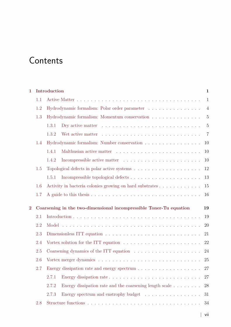
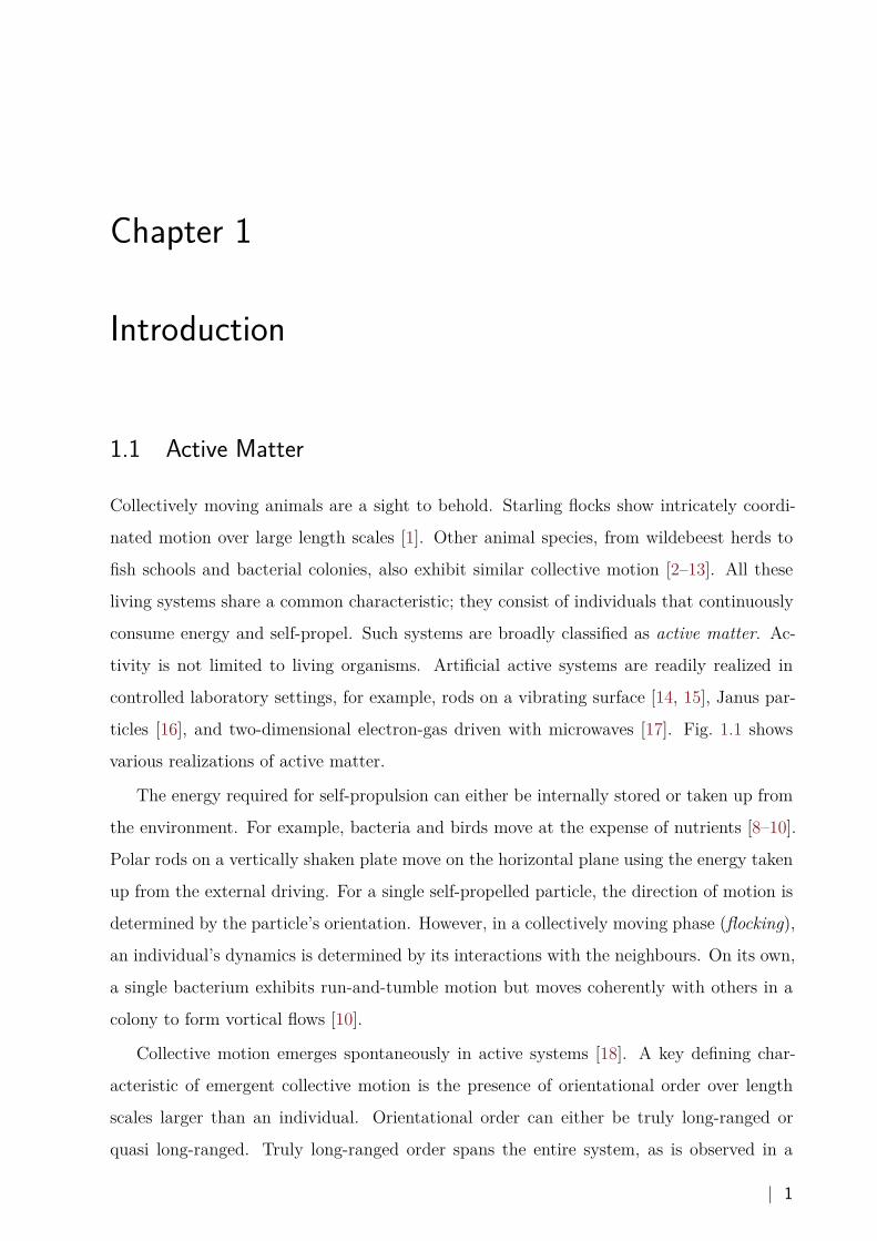
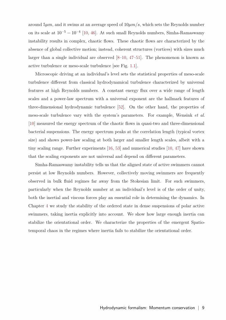
ticles [16], and two-dimensional electron-gas driven with microwaves [17]. Fig. 1.1 shows
various realizations of active matter.
The energy required for self-propulsion can either be internally stored or taken up from
the environment. For example, bacteria and birds move at the expense of nutrients [8–10].
Polar rods on a vertically shaken plate move on the horizontal plane using the energy taken
up from the external driving. For a single self-propelled particle, the direction of motion is
determined by the particle’s orientation. However, in a collectively moving phase (flocking),
an individual’s dynamics is determined by its interactions with the neighbours. On its own,
a single bacterium exhibits run-and-tumble motion but moves coherently with others in a
colony to form vortical flows [10].
Collective motion emerges spontaneously in active systems [18]. A key defining char-
acteristic of emergent collective motion is the presence of orientational order over length
scales larger than an individual. Orientational order can either be truly long-ranged or
quasi long-ranged. Truly long-ranged order spans the entire system, as is observed in a
| 1
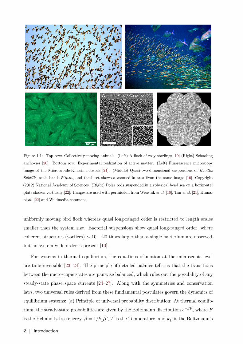
Figure 1.1: Top row: Collectively moving animals. (Left) A flock of rosy starlings [19] (Right) Schooling
anchovies [20]. Bottom row: Experimental realization of active matter. (Left) Fluorescence microscopy
image of the Microtubule-Kinesin network [21]. (Middle) Quasi-two-dimensional suspensions of Bacillis
Subtilis, scale bar is 50𝜇𝑚, and the inset shows a zoomed-in area from the same image [10], Copyright
(2012) National Academy of Sciences. (Right) Polar rods suspended in a spherical bead sea on a horizontal
plate shaken vertically [22]. Images are used with permission from Wensink et al. [10], Tan et al. [21], Kumar
et al. [22] and Wikimedia commons.
uniformly moving bird flock whereas quasi long-ranged order is restricted to length scales
smaller than the system size. Bacterial suspensions show quasi long-ranged order, where
coherent structures (vortices) ∼ 10 − 20 times larger than a single bacterium are observed,
but no system-wide order is present [10].
For systems in thermal equilibrium, the equations of motion at the microscopic level
are time-reversible [23, 24]. The principle of detailed balance tells us that the transitions
between the microscopic states are pairwise balanced, which rules out the possibility of any
steady-state phase space currents [24–27]. Along with the symmetries and conservation
laws, two universal rules derived from these fundamental postulates govern the dynamics of
equilibrium systems: (a) Principle of universal probability distribution: At thermal equilib-
rium, the steady-state probabilities are given by the Boltzmann distribution 𝑒−𝛽𝐹 , where 𝐹is the Helmholtz free energy, 𝛽 = 1/𝑘𝐵𝑇 , 𝑇 is the Temperature, and 𝑘𝐵 is the Boltzmann’s
2 | Introduction
constant. (b) Fluctuation-dissipation theorem: The relation between the fluctuations in a
system and the system’s response to said fluctuations.
Continuous energy intake at an individual’s level breaks the time-reversal symmetry at
the microscopic level and drives active matter out of equilibrium. Consequently, steady
states in active matter do not obey the principle of detailed balance and exhibit constant
mean energy and momentum fluxes [28]. The absence of detailed balance implies that the
fluctuation-dissipation theorem is not valid for such systems. Owing to the continuous
driving, we cannot treat activity as a small perturbation to an equilibrium system. The
equations of motion for an active system are then governed solely by the conservation laws
and the symmetries. The precise nature of non-equilibrium steady states will vary from
system to system [28], but common features like collective motion, steady-state currents, and
topological defects shared by a variety of active systems suggests that a general statistical
framework, independent of the microscopic details, is possible for active systems.
In this thesis, we study the statistical and dynamical properties of dense collections
of polar self-propelled particles using the coarse-grained hydrodynamic description. Active
hydrodynamics, pioneered by Toner and Tu [4], Marchetti et al. [18], Simha and Ramaswamy
[29] and others, has proven to be quite successful in understanding various properties of
active matter. It focuses on the large-time, long-wavelength (average) behaviour of slow
variables of a dynamical system that do not relax to their steady-state values in a finite
time [30, 31]. Examples of slow variables are densities of conserved quantities and broken
symmetry variables. A well known hydrodynamic equation is the equation of continuity
which says that if the total mass in a system is conserved, the local mass density 𝜌(𝐱, 𝑡)can only be altered via density currents. For a simple fluid, mass conservation reads [32]
𝜕𝑡𝜌 + ∇ ⋅ (𝜌𝐮) = 0, (1.1)
where 𝐮 is the fluid velocity.
In the first part of the thesis, we focus on the coarsening dynamics of dense polar ac-
tive matter in the absence of momentum conservation. In the second part, we explore the
stability of the aligned state to perturbations in bulk suspensions of active polar particles,
where the system’s total momentum is conserved. In the final part, we study the spreading
of a bacterial colony growing on a hard agar plate, where the energy-intake does not lead
to self-propulsion, but drives birth-death processes. The rest of this chapter surveys the hy-
drodynamic formalism and previously known results for active systems under consideration
in this thesis. We conclude the chapter with a brief guide to the thesis.
Hydrodynamic formalism: Polar order parameter | 3
1.2 Hydrodynamic formalism: Polar order parameter
Collective motion in active matter is characterized by orientational order, which arises from
alignment interactions between the self-propelled particles. These interactions are either
mechanical, for example, in polar rods [2, 22], or behavioural as observed in a bird flock
[2, 3, 18].
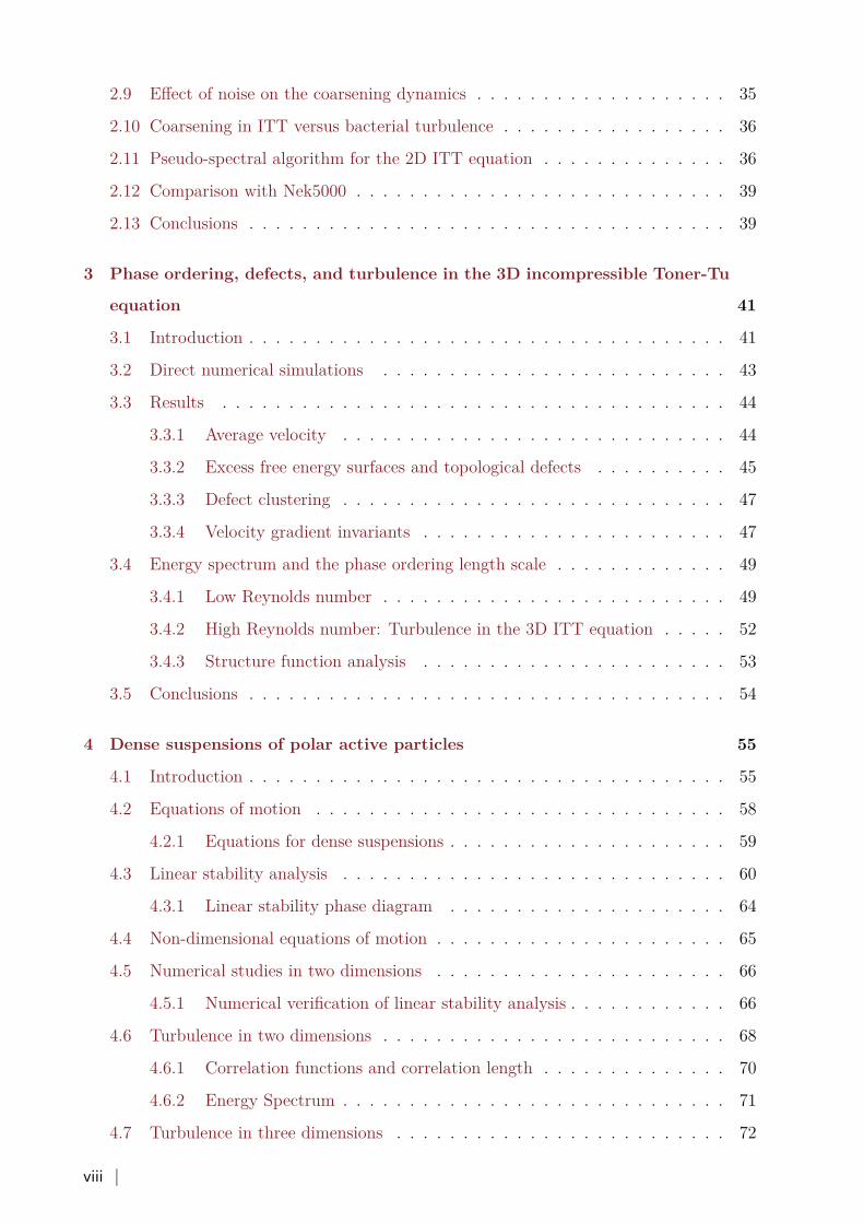
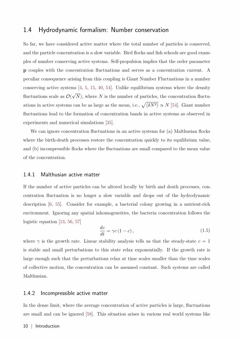
Orientational alignment can either be polar or apolar. Polar individuals have a preferred
sense of direction along the alignment axis that apolar individuals lack. Bird flocks, Bacteria
and Fish schools are polar systems, whereas Microtubules are apolar. Apolarity can also
manifest on macroscopic scales when polar individuals rapidly switch the direction of self-
propulsion as observed in the colonies of Myxobacteria [33].
Figure 1.2: (a) Polar and (b) apolar (nematic) orientational order. Reflection symmetry for the local
orientation is only available for the apolar orientational order. Rotating an arrow by 180∘ does not lead to
the same state, rotating a symmetric rod does.
We are interested in polar active systems, where a vector order parameter 𝐩 measures
the extent of orientational order [2, 29, 34]. 𝐩 = 0 everywhere represents a disordered
phase, whereas 𝐩 = 1 throughout implies a perfect orientational alignment. Orientational
order in active systems emerges spontaneously and a priori, there is no preferred direction
of alignment. A flock can end up orienting in any direction with equal probability [2, 4,
35]. By virtue of this rotational symmetry, the ordered state is invariant under uniform
rotations. The transverse component of the order parameter 𝐩⟂ is then a slow variable with
an infinitely long relaxation time [36]. Note that the longitudinal component of the order
parameter field is not a slow variable as there is no symmetry preventing it from relaxing
back quickly [36].
The reader should note that not all active systems show alignment interactions. For
example, spherical self-propelled colloids do not align with their neighbours [37]. Such
systems are described by a scalar order parameter, namely the density difference between the
liquid and gaseous phase, and show motility induced phase separation [37, 38]. Alignment
interactions are also absent in chiral active fluids, where the activity manifests as a self-
spinning at a constant rate in two dimensions [39]. For a discussion on Nematic, Scalar,
4 | Introduction
and Chiral active systems, we refer the reader to the articles of Ramaswamy [2], Marchetti
et al. [18], Cates and Tailleur [37], Cates and Tjhung [38], and Fürthauer et al. [39].
1.3 Hydrodynamic formalism: Momentum conservation
Based on how the background fluid is treated we can classify active matter into two cate-
gories: (i) dry active matter and (ii) wet active matter.
1.3.1 Dry active matter
Active systems where the background fluid is ignored in the hydrodynamic formalism are
called dry. Typical examples of dry active matter are bird flocks and granular rods on a
vibrating surface. In quiescent conditions, the surrounding air exerts negligible force on a
bird, and we need not consider the motion of the air to understand the dynamics of the bird
flock. For polar rods on a vibrating surface, there is no background fluid present. Another
classic example of a dry active system is the microscopic Vicsek model, where a polar
individual moves at a constant speed and aligns in the average direction of its neighbours,
albeit with some rotational error (noise) [35]. Since the background fluid is ignored in
the hydrodynamic theory, the total momentum of the active particles and the fluid is not
conserved.
The hydrodynamic equations of motion (also known as the Toner-Tu theory in literature)
for dry active matter with conserved number of particles1 are: [4–6, 40]
𝜕𝑡𝑐 + ∇ ⋅ (𝐩𝑐) = 0,
𝜕𝑡𝐩 + 𝜆(𝐩 ⋅ ∇)𝐩 + 𝜆2(∇ ⋅ 𝐩)𝐩 + 𝜆3∇(|𝐩|2) = (𝛼 − 𝛽|𝐩|2)𝐩 − ∇Π − 𝐩(𝐩 ⋅ ∇Π2)
+ 𝐷∇2𝐩 + 𝐷1∇(∇ ⋅ 𝐩) + 𝐷2(𝐩 ⋅ ∇)2𝐩 + 𝜼.(1.2)
Here 𝑐(𝐱, 𝑡) is the local concentration, 𝜆 terms arise from the self-propulsion, Π and Π2
are the pressure terms, 𝐷𝑖 are the diffusion terms, and 𝜼 is the rotational noise. The active
driving term (𝛼−𝛽|𝐩|2) tries to maintain the magnitude of the velocity field at 𝑝0 = √𝛼/𝛽provided 𝛼, 𝛽 > 0. The diffusion terms with coefficients 𝜈, and 𝐷𝑖 represent the tendency
of active particles to follow their neighbors.
In the absence of momentum conservation, (1.2) lack Galilean invariance and contains
terms that are otherwise not allowed for equilibrium systems. For example, for a fluid1We discuss number conservation in active matters in details in Section 1.4
Hydrodynamic formalism: Momentum conservation | 5
described by the Navier-Stokes equation, Galilean invariance forces 𝜆 = 1, 𝜆2 = 𝜆3 = 0,
and the anisotropic pressure term Π2 is forbidden [32].
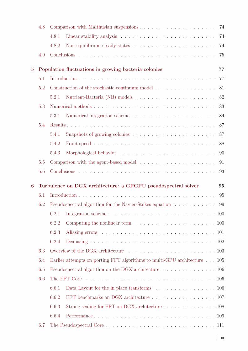
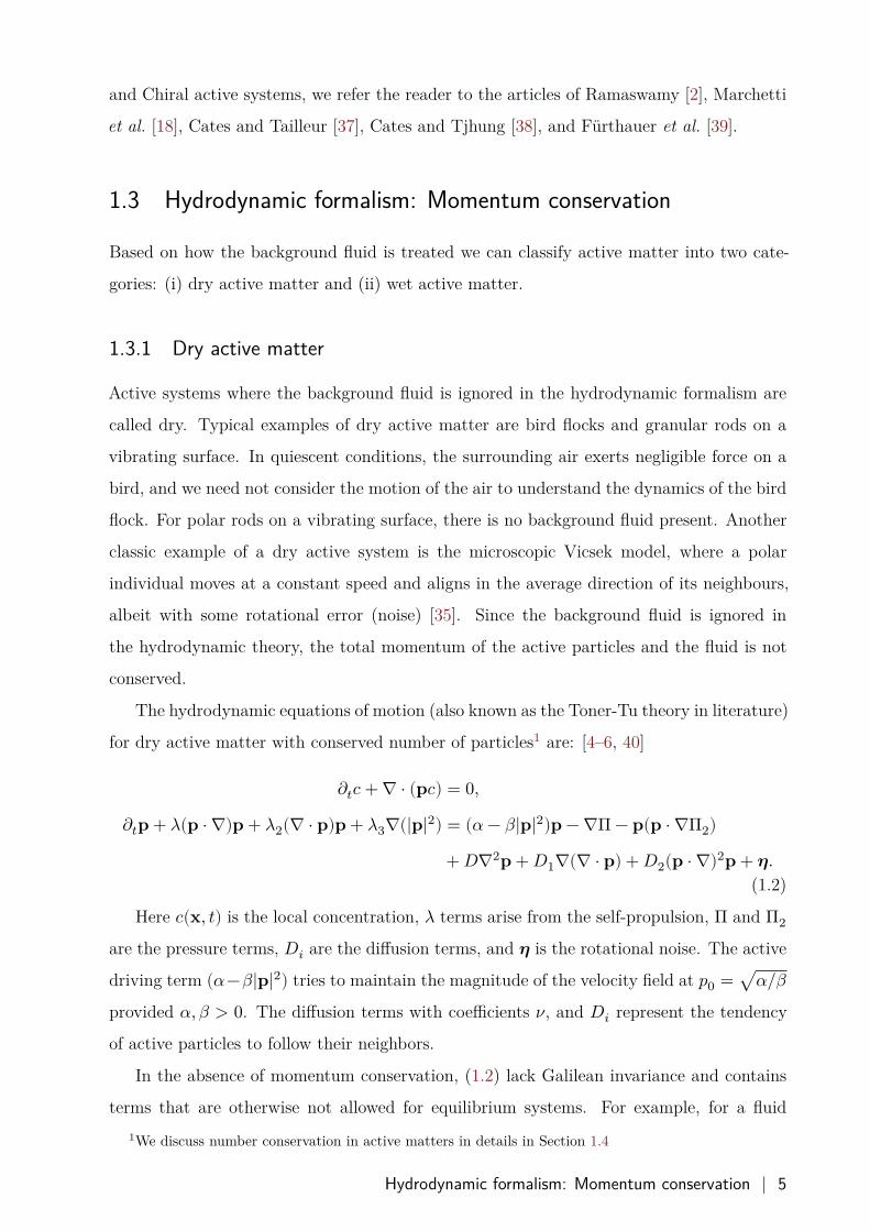
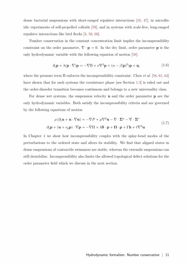
Figure 1.3: Phase diagram for polar dry active systems [34]. Three distinct phases are observed based on
the strength of rotational noise and the mean particle concentration (density), (i) Homogeneous disordered
phase, (ii) Coexistence phase, where dense bands of particles are observed amidst a disordered gaseous
phase, and (iii) An orientationally ordered phase where the entire flock moves collectively. Reprinted with
permission from Chaté [34].
Order-disorder transition
The Toner-Tu hydrodynamic theory and its microscopic variant, the Vicsek model, show
that dry active systems exhibit three distinct phases based on the strength of rotational noise
and the mean particle concentration. At low concentration or high noise, a homogeneous
disordered phase is observed. As the concentration is increased while keeping the noise fixed
(or the noise is decreased keeping the concentration fixed), a coexistence phase emerges,
where dense collectively moving bands are observed amidst a disordered gaseous phase. At
low noise or high concentration an orientationally ordered phase emerges, where the entire
flock moves collectively.
While the order-disorder transition is well understood within the framework of Toner-Tu
theory and the Vicsek model, the coarsening dynamics from the disordered gas-like phase to
the orientationally ordered liquid-like phase is yet to be explored fully. A key challenge in
understanding coarsening in dry active systems arises from the fact that the concentration
and the velocity field are strongly coupled [34, 41–43]. Indeed Mishra et al. [41] used both
the density and the velocity correlations to study coarsening in the TT equations. The
6 | Introduction
authors observed that the coarsening length scale grew faster than equilibrium systems
with the vector order parameter, and argued that the advective nonlinearity accelerates the
coarsening dynamics. However, how nonlinearity alters energy transfer between different
scales remains unanswered. In Chapters 2 and 3 we study the coarsening dynamics of
incompressible polar active matter in two and three dimensions, respectively. In the dense
limit, the fact that the order parameter is the only hydrodynamic variable allows us to
characterize the role of advective nonlinearity in the coarsening dynamics. We show that the
coarsening proceeds via repeated defect merger, and turbulence accelerates the coarsening
dynamics.
1.3.2 Wet active matter
In wet systems, the dynamics of the background fluid flow is explicitly taken into account
[29]. Suspensions of self-propelling swimmers like Escherichia coli [8, 10] and Chlamy-
domonas are typical examples of wet active matter. Here, the swimmers generate stresses
that churn the surrounding fluid. In turn, the fluid flow alters the swimmer orientation and
velocity in a momentum conserving fashion [18, 29, 38].
In the limit of constant suspension density 𝜌, the total mass conservation equation (1.1)
reduces to the incompressibility constraint ∇ ⋅ 𝐮 = 0 for the suspension velocity 𝐮. Further,
momentum conservation gives us the following equations of motion [29, 38]:
𝜕𝑡(𝜌𝐮) = −∇ ⋅ 𝚺,
𝜕𝑡𝐩 + (𝐮 + 𝑣0𝐩) ⋅ ∇𝐩 = 𝜆𝐒 ⋅ 𝐩 + 𝛀 ⋅ 𝐩 + Γ𝐡 + ℓ∇2𝐮,
𝜕𝑡𝑐 + ∇ ⋅ [(𝐮 + 𝑣1𝐩) 𝑐] = 0,
(1.3)
where 𝚺 = 𝑃 𝐈 + 𝜌𝐮𝐮 − 𝜇(∇𝐮 + ∇𝐮𝑇 ) + 𝚺𝑎 + 𝚺𝑟 is the total stress tensor. 𝑃𝐈, 𝜇(∇𝐮 +∇𝐮𝑇 ), and 𝜌𝐮𝐮 are the familiar pressure, viscous and inertial stresses of a Newtonian fluid,
respectively. 𝚺𝑎 = 𝜎𝑎(𝑐)𝐩𝐩 + 𝛾𝑎(𝑐) (∇𝐩 + ∇𝐩𝑇 ) and 𝚺𝑟 = 𝜆+𝐡𝐩 + 𝜆−𝐩𝐡 + ℓ(∇𝐡 + ∇𝐡𝑇 )are the active and restoring stresses arising from swimming activity [18, 29, 38], where
𝜎𝑎(𝑐) > 0(< 0) for extensile (contractile) swimmers [see Fig. 1.4], and 𝛾𝑎 determines the
polar contribution to the active stress.
In the 𝐩 equation, 𝑣0𝐩 is the local velocity of the suspended particles, 𝜆 is the flow
alignment parameter, 𝐒 and 𝛀 are the symmetric and anti-symmetric parts of the velocity
gradient tensor ∇𝐮. 𝐡 = −𝛿𝐹/𝛿𝐩 is the molecular field conjugate to 𝐩 derived from the
Hydrodynamic formalism: Momentum conservation | 7
free-energy functional
𝐹 = ∫ 𝑑3𝑟 [𝐾2 (∇𝐩)2 + 1
4(𝐩.𝐩 − 1)2 − 𝐸𝐩 ⋅ ∇𝑐] . (1.4)
𝐹 favors a uniform ordered state with a unit magnitude. For simplicity, we choose a single
Frank constant 𝐾, which penalizes gradients in 𝐩 [44]. 𝐸 favors the alignment of 𝐩 to up
or down gradients of 𝑐 according to its sign. Γ is the rotational mobility for the relaxation
of the order parameter field, and ℓ governs the lowest-order polar flow-coupling term [45].
𝑣1 is the speed at which the order parameter advects the concentration field.
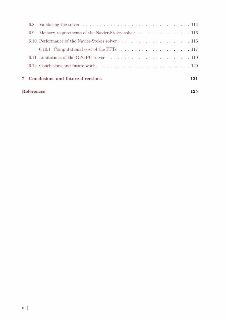
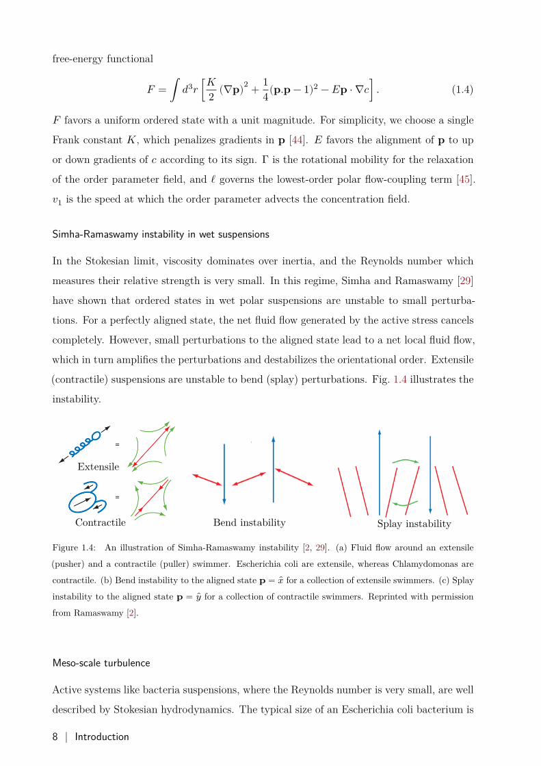
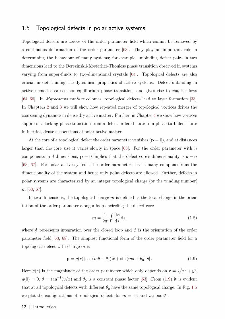
Simha-Ramaswamy instability in wet suspensions
In the Stokesian limit, viscosity dominates over inertia, and the Reynolds number which
measures their relative strength is very small. In this regime, Simha and Ramaswamy [29]
have shown that ordered states in wet polar suspensions are unstable to small perturba-
tions. For a perfectly aligned state, the net fluid flow generated by the active stress cancels
completely. However, small perturbations to the aligned state lead to a net local fluid flow,
which in turn amplifies the perturbations and destabilizes the orientational order. Extensile
(contractile) suspensions are unstable to bend (splay) perturbations. Fig. 1.4 illustrates the
instability.
Figure 1.4: An illustration of Simha-Ramaswamy instability [2, 29]. (a) Fluid flow around an extensile
(pusher) and a contractile (puller) swimmer. Escherichia coli are extensile, whereas Chlamydomonas are
contractile. (b) Bend instability to the aligned state 𝐩 = �� for a collection of extensile swimmers. (c) Splay
instability to the aligned state 𝐩 = 𝑦 for a collection of contractile swimmers. Reprinted with permission
from Ramaswamy [2].
Meso-scale turbulence
Active systems like bacteria suspensions, where the Reynolds number is very small, are well
described by Stokesian hydrodynamics. The typical size of an Escherichia coli bacterium is
8 | Introduction
around 5𝜇𝑚, and it swims at an average speed of 10𝜇𝑚/𝑠, which sets the Reynolds number
on its scale at 10−5 − 10−4 [10, 46]. At such small Reynolds numbers, Simha-Ramaswamy
instability results in complex, chaotic flows. These chaotic flows are characterized by the
absence of global collective motion; instead, coherent structures (vortices) with sizes much
larger than a single individual are observed [8–10, 47–51]. The phenomenon is known as
active turbulence or meso-scale turbulence [see Fig. 1.1].
Microscopic driving at an individual’s level sets the statistical properties of meso-scale
turbulence different from classical hydrodynamical turbulence characterized by universal
features at high Reynolds numbers. A constant energy flux over a wide range of length
scales and a power-law spectrum with a universal exponent are the hallmark features of
three-dimensional hydrodynamic turbulence [52]. On the other hand, the properties of
meso-scale turbulence vary with the system’s parameters. For example, Wensink et al.
[10] measured the energy spectrum of the chaotic flows in quasi-two and three-dimensional
bacterial suspensions. The energy spectrum peaks at the correlation length (typical vortex
size) and shows power-law scaling at both larger and smaller length scales, albeit with a
tiny scaling range. Further experiments [16, 53] and numerical studies [10, 47] have shown
that the scaling exponents are not universal and depend on different parameters.
Simha-Ramaswamy instability tells us that the aligned state of active swimmers cannot
persist at low Reynolds numbers. However, collectively moving swimmers are frequently
observed in bulk fluid regimes far away from the Stokesian limit. For such swimmers,
particularly when the Reynolds number at an individual’s level is of the order of unity,
both the inertial and viscous forces play an essential role in determining the dynamics. In
Chapter 4 we study the stability of the ordered state in dense suspensions of polar active
swimmers, taking inertia explicitly into account. We show how large enough inertia can
stabilize the orientational order. We characterize the properties of the emergent Spatio-
temporal chaos in the regimes where inertia fails to stabilize the orientational order.
Hydrodynamic formalism: Momentum conservation | 9
1.4 Hydrodynamic formalism: Number conservation
So far, we have considered active matter where the total number of particles is conserved,
and the particle concentration is a slow variable. Bird flocks and fish schools are good exam-
ples of number conserving active systems. Self-propulsion implies that the order parameter
𝐩 couples with the concentration fluctuations and serves as a concentration current. A
peculiar consequence arising from this coupling is Giant Number Fluctuations in a number
conserving active systems [4, 5, 15, 40, 54]. Unlike equilibrium systems where the density
fluctuations scale as O(√
𝑁), where 𝑁 is the number of particles, the concentration fluctu-
ations in active systems can be as large as the mean, i.e., √⟨𝛿𝑁2⟩ ∝ 𝑁 [54]. Giant number
fluctuations lead to the formation of concentration bands in active systems as observed in
experiments and numerical simulations [35].
We can ignore concentration fluctuations in an active systems for (a) Malthusian flocks
where the birth-death processes restore the concentration quickly to its equilibrium value,
and (b) incompressible flocks where the fluctuations are small compared to the mean value
of the concentration.
1.4.1 Malthusian active matter
If the number of active particles can be altered locally by birth and death processes, con-
centration fluctuation is no longer a slow variable and drops out of the hydrodynamic
description [6, 55]. Consider for example, a bacterial colony growing in a nutrient-rich
environment. Ignoring any spatial inhomogeneities, the bacteria concentration follows the
logistic equation [13, 56, 57]𝑑𝑐𝑑𝑡 = 𝛾𝑐 (1 − 𝑐) , (1.5)
where 𝛾 is the growth rate. Linear stability analysis tells us that the steady-state 𝑐 = 1is stable and small perturbations to this state relax exponentially. If the growth rate is
large enough such that the perturbations relax at time scales smaller than the time scales
of collective motion, the concentration can be assumed constant. Such systems are called
Malthusian.
1.4.2 Incompressible active matter
In the dense limit, where the average concentration of active particles is large, fluctuations
are small and can be ignored [58]. This situation arises in various real world systems like
10 | Introduction
dense bacterial suspensions with short-ranged repulsive interactions [10, 47], in microflu-
idic experiments of self-propelled colloids [59], and in systems with scale-free, long-ranged
repulsive interactions like bird flocks [3, 58, 60].
Number conservation in the constant concentration limit implies the incompressibility
constraint on the order parameter, ∇ ⋅ 𝐩 = 0. In the dry limit, order parameter 𝐩 is the
only hydrodynamic variable with the following equation of motion [58]:
𝜕𝑡𝐩 + 𝜆(𝐩 ⋅ ∇)𝐩 = −∇Π + 𝜈∇2𝐩 + (𝛼 − 𝛽|𝐩|2)𝐩 + 𝜼, (1.6)
where the pressure term Π enforces the incompressibility constraint. Chen et al. [58, 61, 62]
have shown that for such systems the coexistence phase [see Section 1.3] is ruled out and
the order-disorder transition becomes continuous and belongs to a new universality class.
For dense wet systems, the suspension velocity 𝐮 and the order parameter 𝐩 are the
only hydrodynamic variables. Both satisfy the incompressibility criteria and are governed
by the following equations of motion
𝜌 (𝜕𝑡𝐮 + 𝐮 ⋅ ∇𝐮) = −∇𝑃 + 𝜇∇2𝐮 − ∇ ⋅ 𝚺𝑎 − ∇ ⋅ 𝚺𝑟
𝜕𝑡𝐩 + (𝐮 + 𝑣0𝐩) ⋅ ∇𝐩 = −∇Π + 𝜆𝐒 ⋅ 𝐩 + 𝛀 ⋅ 𝐩 + Γ𝐡 + ℓ∇2𝐮.(1.7)
In Chapter 4 we show how incompressibility couples with the splay-bend modes of the
perturbations to the ordered state and alters its stability. We find that aligned states in
dense suspensions of contractile swimmers are stable, whereas the extensile suspensions can
still destabilize. Incompressibility also limits the allowed topological defect solutions for the
order parameter field which we discuss in the next section.
Hydrodynamic formalism: Number conservation | 11
1.5 Topological defects in polar active systems
Topological defects are zeroes of the order parameter field which cannot be removed by
a continuous deformation of the order parameter [63]. They play an important role in
determining the behaviour of many systems; for example, unbinding defect pairs in two
dimensions lead to the Berezinskii-Kosterlitz-Thouless phase transition observed in systems
varying from super-fluids to two-dimensional crystals [64]. Topological defects are also
crucial in determining the dynamical properties of active systems. Defect unbinding in
active nematics causes non-equilibrium phase transitions and gives rise to chaotic flows
[64–66]. In Myxococcus xanthus colonies, topological defects lead to layer formation [33].
In Chapters 2 and 3 we will show how repeated merger of topological vortices drives the
coarsening dynamics in dense dry active matter. Further, in Chapter 4 we show how vortices
suppress a flocking phase transition from a defect-ordered state to a phase turbulent state
in inertial, dense suspensions of polar active matter.
At the core of a topological defect the order parameter vanishes (𝐩 = 0), and at distances
larger than the core size it varies slowly in space [63]. For the order parameter with 𝑛components in 𝑑 dimensions, 𝐩 = 0 implies that the defect core’s dimensionality is 𝑑 − 𝑛[63, 67]. For polar active systems the order parameter has as many components as the
dimensionality of the system and hence only point defects are allowed. Further, defects in
polar systems are characterized by an integer topological charge (or the winding number)
𝑚 [63, 67].
In two dimensions, the topological charge 𝑚 is defined as the total change in the orien-
tation of the order parameter along a loop encircling the defect core
𝑚 = 12𝜋 ∮ d𝜙
d𝑠 d𝑠, (1.8)
where ∮ represents integration over the closed loop and 𝜙 is the orientation of the order
parameter field [63, 68]. The simplest functional form of the order parameter field for a
topological defect with charge 𝑚 is
𝐩 = 𝑔(𝑟) [cos (𝑚𝜃 + 𝜃0) 𝑥 + sin (𝑚𝜃 + 𝜃0) 𝑦] . (1.9)
Here 𝑔(𝑟) is the magnitude of the order parameter which only depends on 𝑟 = √𝑥2 + 𝑦2,
𝑔(0) = 0, 𝜃 = tan−1(𝑦/𝑥) and 𝜃0 is a constant phase factor [63]. From (1.9) it is evident
that at all topological defects with different 𝜃0 have the same topological charge. In Fig. 1.5
we plot the configurations of topological defects for 𝑚 = ±1 and various 𝜃0.
12 | Introduction
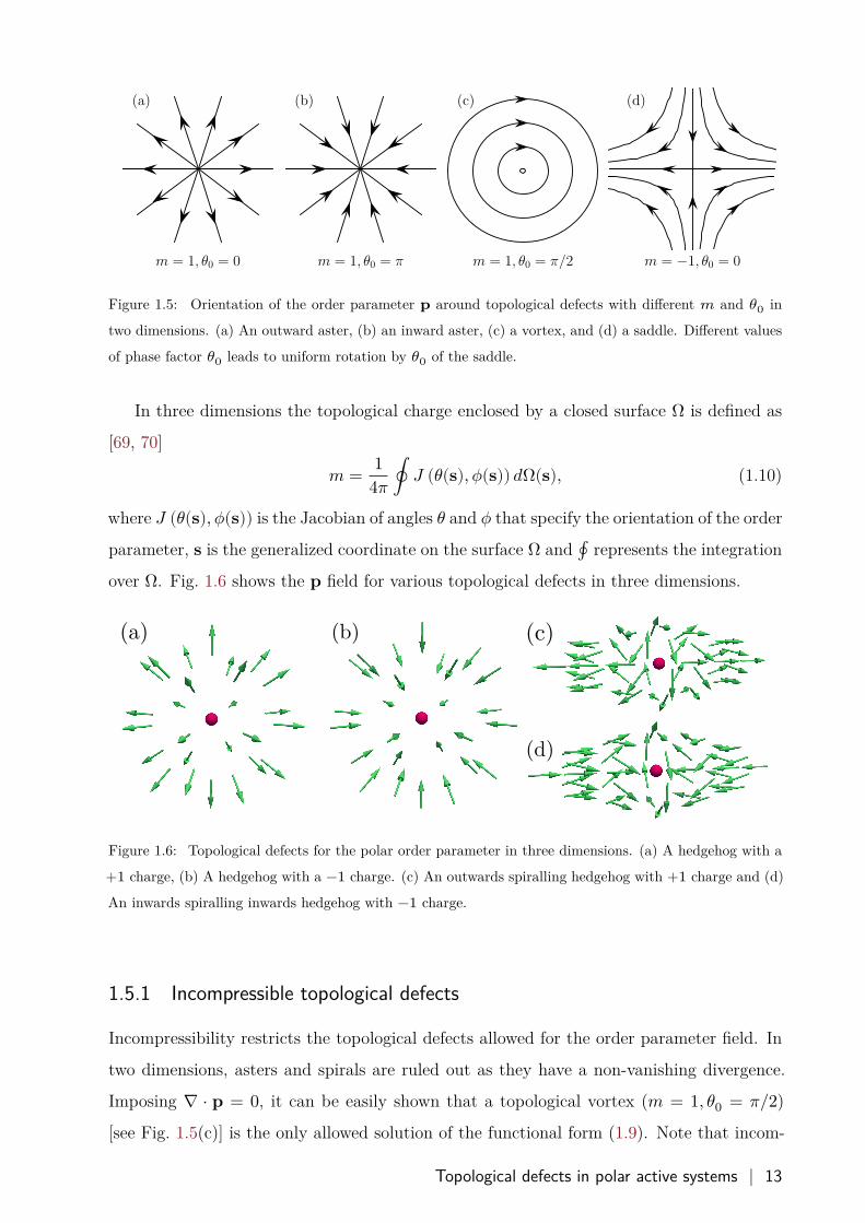
Figure 1.5: Orientation of the order parameter 𝐩 around topological defects with different 𝑚 and 𝜃0 in
two dimensions. (a) An outward aster, (b) an inward aster, (c) a vortex, and (d) a saddle. Different values
of phase factor 𝜃0 leads to uniform rotation by 𝜃0 of the saddle.
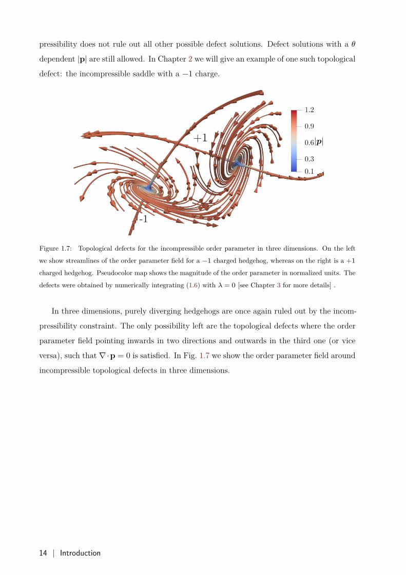
In three dimensions the topological charge enclosed by a closed surface Ω is defined as
[69, 70]
𝑚 = 14𝜋 ∮ 𝐽 (𝜃(𝐬), 𝜙(𝐬)) 𝑑Ω(𝐬), (1.10)
where 𝐽 (𝜃(𝐬), 𝜙(𝐬)) is the Jacobian of angles 𝜃 and 𝜙 that specify the orientation of the order
parameter, 𝐬 is the generalized coordinate on the surface Ω and ∮ represents the integration
over Ω. Fig. 1.6 shows the 𝐩 field for various topological defects in three dimensions.
Figure 1.6: Topological defects for the polar order parameter in three dimensions. (a) A hedgehog with a
+1 charge, (b) A hedgehog with a −1 charge. (c) An outwards spiralling hedgehog with +1 charge and (d)
An inwards spiralling inwards hedgehog with −1 charge.
1.5.1 Incompressible topological defects
Incompressibility restricts the topological defects allowed for the order parameter field. In
two dimensions, asters and spirals are ruled out as they have a non-vanishing divergence.
Imposing ∇ ⋅ 𝐩 = 0, it can be easily shown that a topological vortex (𝑚 = 1, 𝜃0 = 𝜋/2)
[see Fig. 1.5(c)] is the only allowed solution of the functional form (1.9). Note that incom-
Topological defects in polar active systems | 13
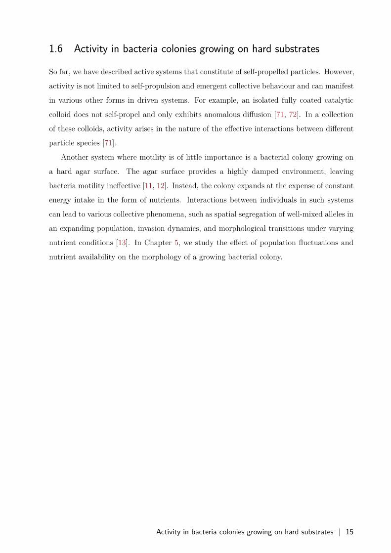
pressibility does not rule out all other possible defect solutions. Defect solutions with a 𝜃dependent |𝐩| are still allowed. In Chapter 2 we will give an example of one such topological
defect: the incompressible saddle with a −1 charge.
Figure 1.7: Topological defects for the incompressible order parameter in three dimensions. On the left
we show streamlines of the order parameter field for a −1 charged hedgehog, whereas on the right is a +1charged hedgehog. Pseudocolor map shows the magnitude of the order parameter in normalized units. The
defects were obtained by numerically integrating (1.6) with 𝜆 = 0 [see Chapter 3 for more details] .
In three dimensions, purely diverging hedgehogs are once again ruled out by the incom-
pressibility constraint. The only possibility left are the topological defects where the order
parameter field pointing inwards in two directions and outwards in the third one (or vice
versa), such that ∇⋅𝐩 = 0 is satisfied. In Fig. 1.7 we show the order parameter field around
incompressible topological defects in three dimensions.
14 | Introduction
1.6 Activity in bacteria colonies growing on hard substrates
So far, we have described active systems that constitute of self-propelled particles. However,
activity is not limited to self-propulsion and emergent collective behaviour and can manifest
in various other forms in driven systems. For example, an isolated fully coated catalytic
colloid does not self-propel and only exhibits anomalous diffusion [71, 72]. In a collection
of these colloids, activity arises in the nature of the effective interactions between different
particle species [71].
Another system where motility is of little importance is a bacterial colony growing on
a hard agar surface. The agar surface provides a highly damped environment, leaving
bacteria motility ineffective [11, 12]. Instead, the colony expands at the expense of constant
energy intake in the form of nutrients. Interactions between individuals in such systems
can lead to various collective phenomena, such as spatial segregation of well-mixed alleles in
an expanding population, invasion dynamics, and morphological transitions under varying
nutrient conditions [13]. In Chapter 5, we study the effect of population fluctuations and
nutrient availability on the morphology of a growing bacterial colony.
Activity in bacteria colonies growing on hard substrates | 15
1.7 A guide to this thesis
This section provides a summary of the rest of the chapters in this thesis.
In Chapter 2, we investigate the coarsening dynamics in two-dimensional dry incom-
pressible polar active matter, where the order parameter is the only dynamical variable
[58, 62]. We show that coarsening proceeds via vortex merger events, and the dynamics
crucially depend on the Reynolds number Re. For low Re, the coarsening process has sim-
ilarities to Ginzburg-Landau dynamics. On the other hand, for high Re, coarsening shows
signatures of turbulence. In particular, we show the presence of an enstrophy cascade from
the inter-vortex separation scale to the dissipation scale. Although the coarsening dynamics
is Re dependent, we show that defects are uniformly distributed throughout the domain,
and dynamical scaling holds at all Re.
In Chapter 3, we study coarsening dynamics in three-dimensional dry incompressible
polar active matter. As was observed in two-dimensions, the transient states en route to
the global order are turbulent. We observe a forward energy cascade and a Kolmogorov
energy spectra and once again, turbulence accelerates the coarsening dynamics. However,
the defect distribution changes as we vary Re. At low Re defects are uniformly distributed
but show clustering at high Re. Further, dynamical scaling holds only at low Re and we
observe that multiple, interacting length scales govern the coarsening dynamics at high Re.
In Chapter 4, we study dense wet suspensions of active polar particles in two and three-
dimensions. We investigate the instabilities of the aligned state to small perturbations
and show how inertia can stabilize the orientational order in incompressible suspensions of
extensile swimmers. We find that a non-dimensional parameter 𝑅 characterizes the stability
of the aligned state. At small 𝑅, the instabilities in the ordered state exhibit a growth rate
proportional to O(𝑞). After a threshold value of 𝑅 = 𝑅1, the instabilities grow at a rate
proportional to O(𝑞2). Past a second threshold value 𝑅 = 𝑅2, the flock is stable. We further
characterize the properties of the spatio-temporal chaos resulting from the instabilities. We
show that, for all 𝑅 < 𝑅2, the flow is riddled with topological vortices with no global order
in sight. Further, the inter-defect spacing grows with 𝑅 and in two dimensions, appears to
diverge at 𝑅 = 𝑅2.
In Chapter 5 we focus on bacterial colonies growing on a hard agar surface. We investi-
gate how population fluctuations and nutrient availability can affect the morphology of grow-
ing bacterial colony. We find that the population fluctuations and nutrient-dependent bac-
16 | Introduction
teria diffusion are sufficient to cause the morphological transition from finger-like branched
fronts to smooth fronts upon increasing nutrient concentration.
In Chapter 6 we present the numerical methods used in this thesis. The chapter focuses
on a general-purpose GPU based (GPGPU) pseudospectral solver for the Navier-Stokes
equation in three dimensions. First, we describe the pseudospectral algorithm and its
GPGPU implementation. We then discuss the performance of the pseudospectral algorithm
on a high bandwidth GPGPU architecture. We will show how the high bandwidth GPGPU
architecture is an ideal platform to perform discrete numerical simulations of the Navier-
Stokes equation at moderate resolutions of size 5123 − 20483 in three dimensions.
In the Chapter 7 we conclude the thesis and outline possible future research directions.
A guide to this thesis | 17

Chapter 2
Coarsening in the two-dimensional incompress-ible Toner-Tu equation
In this chapter, we investigate the coarsening dynamics in the two-dimensional, incompress-
ible Toner-Tu equation. We show that coarsening proceeds via vortex merger events, and the
dynamics crucially depend on the Reynolds number Re. For low Re, the coarsening process
has similarities to Ginzburg-Landau dynamics. On the other hand, for high Re, coarsening
shows signatures of turbulence. In particular, we show the presence of an enstrophy cascade
from the inter-vortex separation scale to the dissipation scale.
2.1 Introduction
Active matter theories have made remarkable progress in understanding the dynamics of
active suspension of polar particles (SPP) such as fish schools, locust swarms, and bird
flocks [2, 18, 73]. The particle based Vicsek model [35] and the hydrodynamic Toner-Tu
(TT) equation [5] provide the simplest setting to investigate the dynamics of SPP. Variants
of the TT equation have been used to model bacterial turbulence [10] and pattern forma-
tion in active fluids [74–77]. An important prediction of these theories is the presence of
a liquid-gas-like transition from a disordered gas phase to an orientationally ordered liquid
phase [2, 34, 37]. This picture is dramatically altered if the density fluctuations are sup-
pressed by imposing an incompressibility constraint. Chen et al. [58, 61], using dynamical
renormalization group studies, showed that for the incompressible Toner-Tu (ITT) equation
the order-disorder transition becomes continuous. The near ordered state of the wet SPP
on a substrate or under confinement [45, 58, 59] belongs to the same universality class as
| 19
the two-dimensional (2D) ITT equation.
Investigating coarsening dynamics from a disordered state to an ordered state in sys-
tems showing phase transitions has been the subject of intense investigation [78–83]. In
active-matter coarsening has been studied either in systems showing motility-induced phase
separation [37, 84] or for dry aligning dilute active matter (DADAM) [34, 41–43]. A key
challenge in understanding coarsening in DADAM comes from the fact that the density
and the velocity field are strongly coupled to each other. Indeed, in [41] the authors used
both the density and the velocity correlations to study coarsening in the TT equation. The
authors observed that the coarsening length scale grew faster than equilibrium systems with
the vector order parameter and argued that the accelerated dynamics are because of the
advective nonlinearity in the TT equation. However, how nonlinearity alters energy transfer
between different scales remains unanswered.
The incompressible limit, where the velocity field is the only dynamical variable, provides
an ideal platform to investigate the role of advection. Therefore, in this paper, we investigate
coarsening dynamics using the ITT equation [58]:
𝜕𝑡𝐮 + 𝜆𝐮 ⋅ ∇𝐮 = −∇𝑃 + 𝜈∇2𝐮 + (𝛼 − 𝛽|𝐮|2) 𝐮. (2.1)
Here 𝐮(𝐱, 𝑡) is the velocity (or the order parameter) field at position 𝐱 and time 𝑡, 𝜆 is
the advection coefficient, 𝜈 is the viscosity, and (𝛼 − 𝛽|𝐮|2) 𝐮 is the active driving term with
coefficients 𝛼, 𝛽 > 0. The pressure 𝑃(𝐱, 𝑡) enforces the incompressibility criterion ∇⋅𝐮 = 0.
We do not consider the random driving term in (2.3) because we are interested in
coarsening under a sudden quench to zero noise. For 𝜆 = 0 and in the absence of pressure
term, (2.3) reduces to the Ginzburg-Landau (GL) equation. On the other hand, (2.3)
reduces to the Navier-Stokes (NS) equation on fixing 𝛼 = 0, 𝛽 = 0, and 𝜆 = 1. Since most
of the dry active matter studies are done on a substrate, we investigate coarsening in two
spatial dimensions.
2.2 Model
We begin by writing down the hydrodynamic equations for dry active matter on a substrate,
which acts as a momentum sink and provides a preferred frame of reference1. The governing
equations of motion for the coarse grained velocity field 𝐮(𝐱, 𝑡) and the density field 𝜌(𝐱, 𝑡)are determined by the conservation laws and the symmetries of the system [4, 36, 40]2. For
1Particles move relative to the surface.2For an excellent pedagogical review see [36].
20 | Coarsening in the two-dimensional incompressible Toner-Tu equation
dry active matter, in the absence of any birth and death processes, there is only one conser-
vation law; the density remains conserved. The system also possesses complete rotational
symmetry as the active particles are equally likely to move in any direction on the substrate.
The equations of motion then are
𝜕𝑡𝜌 + ∇ ⋅ (𝐮𝜌) = 0,
𝜕𝑡𝐮 + 𝜆(𝐮 ⋅ ∇)𝐮 + 𝜆2(∇ ⋅ 𝐮)𝐮 + 𝜆3∇(|𝐮|2) = (𝛼 − 𝛽|𝐮|2)𝐮 − ∇𝑃1 − 𝐮(𝐮 ⋅ ∇𝑃2)
+ 𝜈∇2𝐮 + 𝐷1∇(∇ ⋅ 𝐮) + 𝐷2(𝐮 ⋅ ∇)2𝐮 + 𝜼.(2.2)
As the system is not Galilean invariant, (2.2) contains terms that are otherwise not allowed
for equilibrium systems. For example, for a fluid described by the Navier-Stokes equation,
Galilean invariance forces 𝜆 = 1, 𝜆2,3 = 0, and the anisotropic pressure term (𝑃2) is
forbidden. The active driving term (𝛼 − 𝛽|𝐮|2) tries to maintain the magnitude of the
velocity field at 𝑈 = √𝛼/𝛽 provided 𝛼, 𝛽 > 0. The diffusion terms with coefficients 𝜈, and
𝐷𝑖 represent the tendency of active particles to follow their neighbors. 𝜼 is the noise term
which represents fluctuations in the system. All the parameters, in general, are functions
of the density field 𝜌 and the magnitude of the velocity field |𝐮|.For dense systems on a substrate, we can assume that the particle density is uniform and
constant. In this case, the conservation equation reduces to the incompressibility constraint
∇ ⋅ 𝐮 = 0 that is enforced by the pressure term −∇𝑃 , where 𝑃 = 𝑃1 + 𝜆3|𝐮|2. 𝜆2 and
𝐷1 terms also drop out due to the incompressibility constraint and the parameters 𝜆, 𝛼, 𝛽,
and 𝜈 will only depend on the magnitude of the local velocity |𝐮|, for simplicity we assume
them to be constants. We further drop the anisotropic pressure and diffusion terms to keep
our analysis simple and arrive at the incompressible Toner-Tu equation (ITT)
𝜕𝑡𝐮 + 𝜆(𝐮 ⋅ ∇)𝐮 = −∇𝑃 + 𝜈∇2𝐮 + (𝛼 − 𝛽|𝐮|2)𝐮 + 𝜼. (2.3)
Since we are interested in coarsening dynamics of disordered configurations quenched to
zero temperature, we will ignore the noise term in the following discussion. We discuss the
effect of the noise on the coarsening dynamics in Section 2.9.
2.3 Dimensionless ITT equation
In this section, we write down the dimensionless form of the ITT equation and enumerate
the dimensionless numbers that govern its characteristics. We rescale the space 𝐱′ → 𝐱/𝐿,
Dimensionless ITT equation | 21
the time 𝑡′ → 𝛼𝑡, the velocity field 𝐮′ → 𝐮/𝑈 , and the pressure 𝑃 ′ → 𝑃/𝛼𝐿𝑈 , to get
𝛼𝑈𝜕𝑡′𝐮′ + 𝜆𝑈2
𝐿 𝐮′ ⋅ ∇′𝐮′ = −𝛼𝑈∇′𝑃 ′ + 𝜈𝑈𝐿2 ∇′2𝐮′ + (𝛼 − 𝛽𝑈2|𝐮′|2) 𝑈𝐮′.
Here 𝐿 is the box length and 𝑈2 = 𝛼/𝛽. Ignoring the primed index for convenience, we
arrive at the dimensionless form of the ITT equation
𝜕𝑡𝐮 + ReCn2𝐮 ⋅ ∇𝐮 = −∇𝑃 + Cn2∇2𝐮 + (1 − |𝐮|2) 𝐮.
Here Re ≡ 𝜆𝐿𝑈/𝜈 is the Reynolds number, Cn ≡ ℓ𝑐2/𝐿2 is the Cahn number, and ℓ𝑐 =
√𝜈/𝛼 is the length scale above which fluctuations in the homogeneous disordered state
𝐮 = 0 are linearly unstable3. The ITT equation is then entirely characterized by Re and
Cn.
2.4 Vortex solution for the ITT equation
In this section, we will discussion the topological defect solutions for the ITT equation. The
2D Ginzburg-Landau equation
𝜕𝑡𝐮 = Cn2∇2𝐮 + (1 − |𝐮|2)𝐮, (2.4)
allows for topological defect solutions of the form
𝐮(𝑟, 𝜃) = 𝑓(𝑟) [cos(𝑚𝜃 + 𝜙) 𝑥 + sin(𝑚𝜃 + 𝜙) 𝑦] . (2.5)
Here (𝑟, 𝜃) are the polar coordinates, ( 𝑥, 𝑦) are the unit vectors in Cartesian coordinates,
𝜙 is a constant phase, and 𝑚 is the winding number of the defect. Although, any integer
winding number satisfies (2.4), defects with higher winding number (|𝑚| > 1) are unstable
and decay down to defects with 𝑚 = ±1 [63, 85]. In Fig. 1.5 we plot the velocity field for
different configurations for 𝑚 = ±1. To get the governing equation for 𝑓(𝑟), we set 𝑚 = 1,
and 𝜙 = 0 in (2.5) . The equation for the radial component of the velocity field readily
gives
Cn2 (𝑓 ′′ + 𝑓 ′
𝑟 − 𝑓𝑟2 ) + (1 − 𝑓2)𝑓 = 0. (2.6)
Here the superscript ′ indicates derivatives with respect to 𝑟, and the boundary conditions
are 𝑓(0) = 0, and 𝑓 ′(1) = 0.
For the ITT equation, the nonlinear advection term and the incompressibility constraint
impose additional restrictions on the allowed defect solutions. In particular, ∇ ⋅ 𝐮 = 0 rules3Alternatively, ℓ𝑐 is also the core radius of the vortex defect.
22 | Coarsening in the two-dimensional incompressible Toner-Tu equation
out all other solutions for 𝑚 = 1 except when 𝜙 = ±𝜋/2. It means that vortices are the only
positively charged solutions allowed for the ITT equation. For 𝑚 = −1, no incompressible
solutions of the form (2.5) exist, although other topological charges with 𝑚 = −1 are not
ruled out.
0.0 0.1 0.2 0.3 0.4 0.5 0.6 0.7r
0.0
0.2
0.4
0.6
0.8
1.0f
(r)
Cn = 1.0× 10⁻¹
Cn = 3.2× 10⁻²
Cn = 1.0× 10⁻²
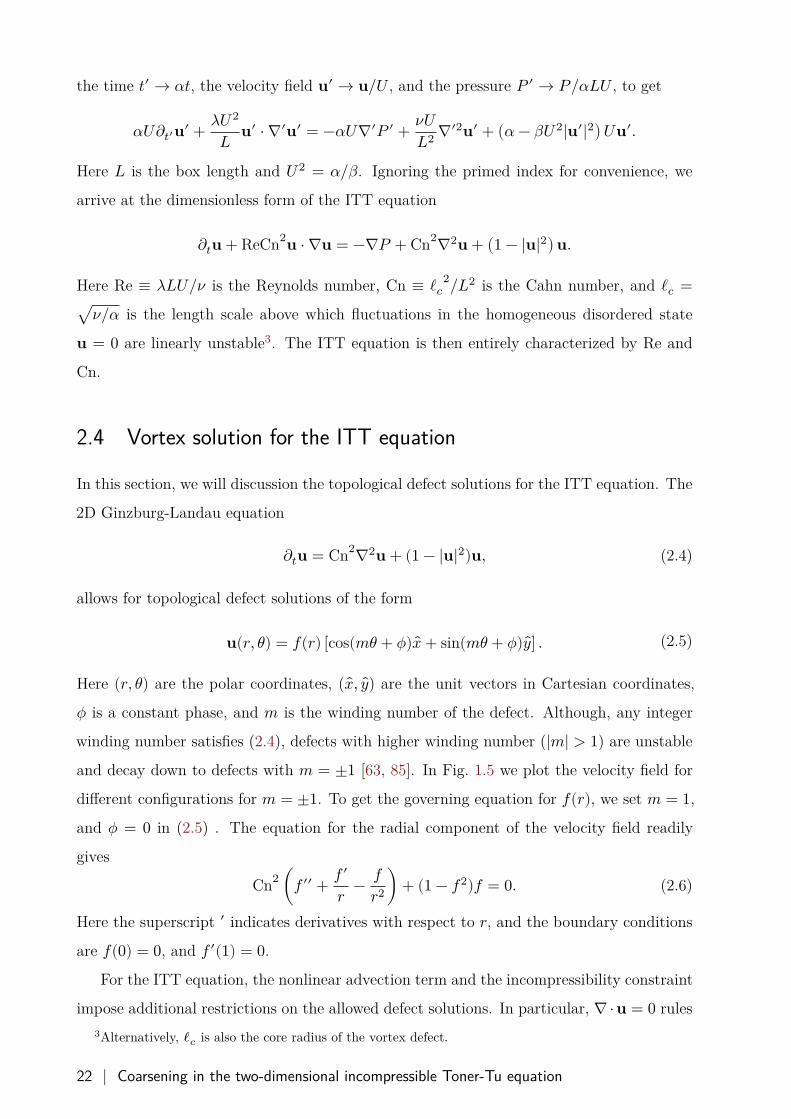
Figure 2.1: Plot of 𝑓(𝑟) vs 𝑟 for different values of Cn.
Consider now the radially symmetric velocity field of an isolated unbounded vortex
𝐮(𝐱, 𝑡) ≡ 𝑓(𝑟) 𝜃, where 𝜃 is the unit vector along the angular direction. Substituting in the
ITT equation, we get the following equations
(𝑓 ′′ + 𝑓 ′
𝑟 − 𝑓𝑟2 ) = 1
Cn2 (𝑓2 − 1)𝑓,
𝑃 (𝑟) = ReCn2 ∫𝑟
0
𝑓2(𝑠)𝑠 𝑑𝑠.
(2.7)
The ITT equation thus admits vortex solutions with pressure being a function of radius 𝑟only. Note that equation for 𝑓(𝑟) does not depend on Re and is identical to the equation of
an isolated defect in the Ginzburg-Landau equation (2.6). In Fig. 2.1 we plot the numerical
solution of 𝑓(𝑟) for different values of Cn. For Cn << 1, a regular perturbation analysis
reveals that 𝑓(𝑟) → 𝐴𝑟(1 − 𝑟2/8Cn2).
Vortex solution for the ITT equation | 23
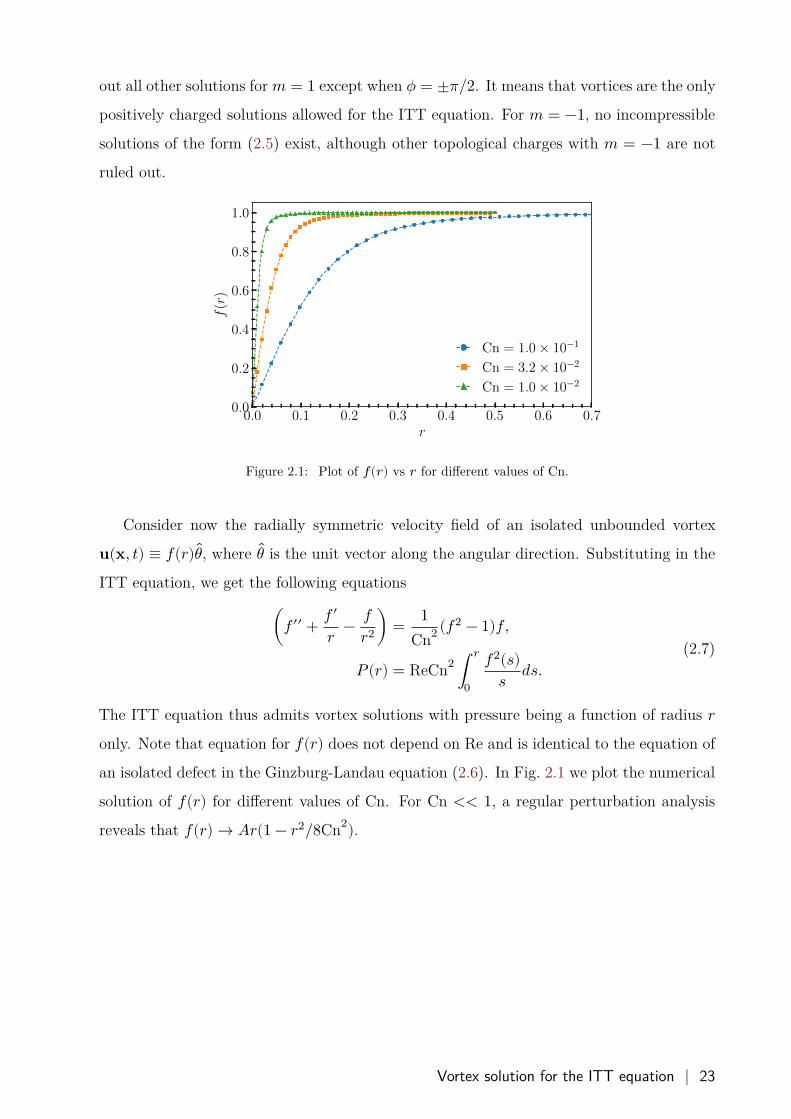
2.5 Coarsening dynamics of the ITT equation
We will now present the results from our study of the coarsening dynamics of (2.3). We use
a pseudospectral method in the stream function-vorticity formulation [86, 87] to perform
direct numerical simulation (DNS) of (2.3) in a periodic square box of side length 𝐿, and
discretize the simulation domain with 𝑁2 collocation points. Unless stated otherwise, we
set 𝐿 = 2𝜋 and 𝑁 = 2048. For details of the numerical methods, see Section 2.11.
(a)
(b)
Figure 2.2: Pseudocolor plots of the vorticity field 𝜔 = 𝑧 ⋅ ∇ × 𝐮 superimposed on the velocity streamlines
at different times for (a) Re = 2𝜋 × 102, and (b) Re = 2𝜋 × 104 in the coarsening regime.
To investigate the coarsening dynamics of the ITT equation, we initialize our simu-
lations in a disordered configuration of randomly oriented velocity vectors drawn from a
Gaussian distribution with zero mean and standard deviation 𝜎 = 𝑈/3. The pseudocolor
plot of the vorticity field in Fig. 2.2(a) and (b) shows different stages of coarsening at
low (Re = 2𝜋 × 102) and high (Re = 2𝜋 × 104) Reynolds number respectively. During
the coarsening, vortices merge, and the inter-vortex spacing continues increasing. For low
Re [see Fig. 2.2(a)], the dynamics in the coarsening regime resembles defect dynamics in
the Ginzburg-Landau equation [79, 82, 88]. On the other hand, for high Re, the vorticity
snapshots resemble 2D turbulence. In particular, similar to vortex merger events in 2D
[89, 90], it is easy to identify a pair of co-rotating vortices undergoing a merger and the
surrounding filamentary structure. Earlier studies on the vortex merger in two-dimensional
Navier-Stokes equations have showed that the filamentary structures formed during the
merger process lead to an enstrophy cascade. Because the ITT equation structure is similar
24 | Coarsening in the two-dimensional incompressible Toner-Tu equation
to NS equations we expect that the vortex merger at high Re will also lead to an enstrophy
cascade.
2.6 Vortex merger dynamics
To investigate the merger of two co-rotating vortices, we perform a DNS of an isolated
vortex-saddle-vortex configuration at various Reynolds numbers. We use a square domain
of area 𝐿2 = 4𝜋2 and discretize it with 𝑁2 = 40962 collocation points. Furthermore, to
minimize the effect of periodic boundaries, we set 𝛼 = −10 for 𝑟 > 0.9𝐿/2 and keep 𝛼 = 1otherwise, where 𝑟 ≡ √(𝑥 − 𝐿/2)2 + (𝑦 − 𝐿/2)2. This ensures that the velocity decays to
zero for 𝑟 ≥ 0.9𝐿/2. The initial condition constitutes a saddle at the center of the square
domain, and two vortices placed at coordinates [(𝐿 − 1)/2, 𝐿/2] and [(𝐿 + 1)/2, 𝐿/2]. It is
important to note that
• Similar to the GL equation [63, 88, 91], vortices in ITT have a topological charge,
• Similar to the NS equation [92], the ITT equation has an advective nonlinearity and
the presence of pressure leads to non-local interactions.
In Fig. 2.3(a)-(e), we plot vorticity contours during different stages of the vortex merger for
different Re. Since the saddle is at equal distance away from the two vortices, its position
does not change during evolution. For low Re = 0, the vortex dynamics has similarities
to the over-damped motion of defects with opposite topological charge in the Ginzburg-
Landau equation. Vortices get attracted to the saddle and move along a straight-line path.
On increasing Re ≥ 2𝜋 × 102, similar to Navier-Stokes, advective nonlinearity in the ITT
becomes crucial. Not only are the vortices attracted to the saddle, but they also go around
each other. The flexure of the vortex trajectory also depends on the Reynolds number.
Thus a vortex merger event in the two-dimensional ITT equation has ingredients both from
the NS and the GL equations.
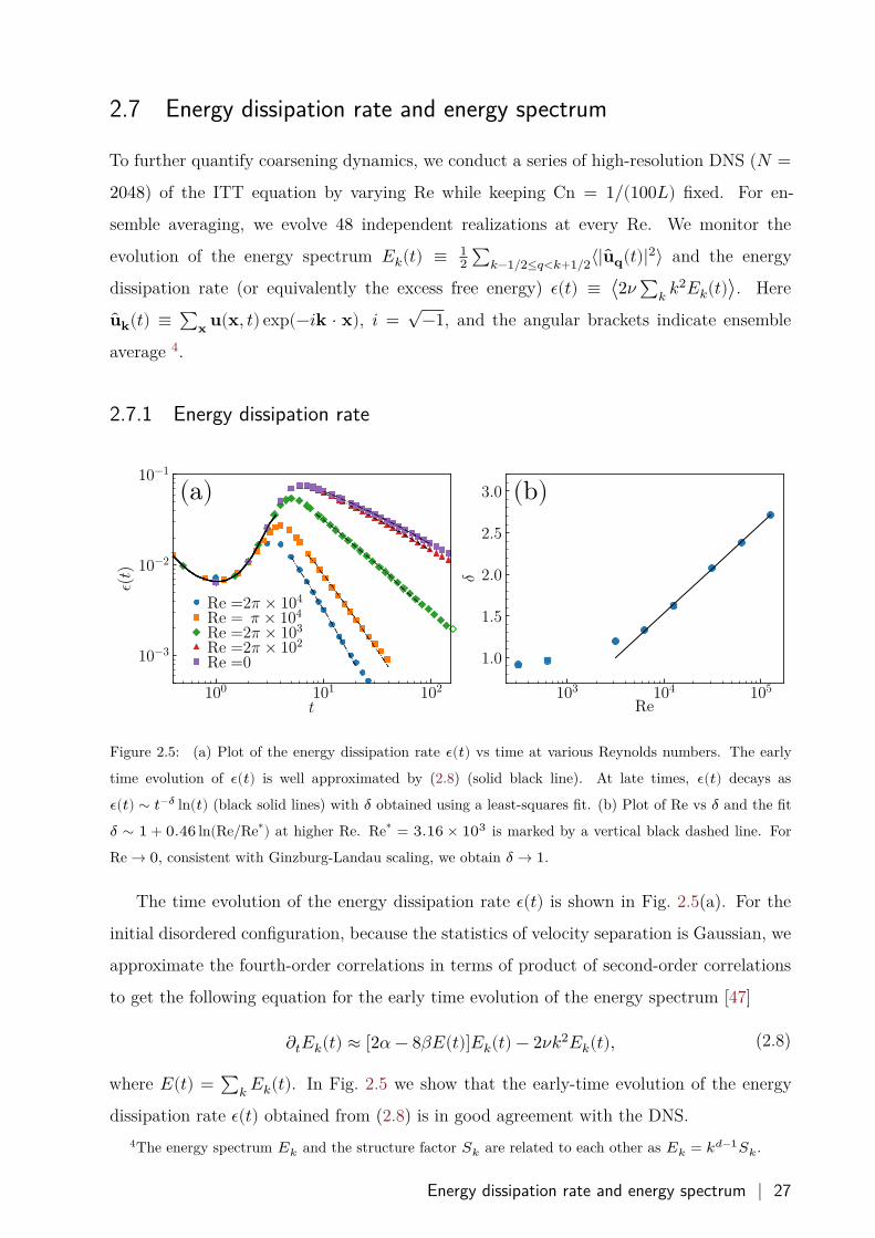
In Fig. 2.4(a) we plot the inter-vortex separation 𝑑(𝑡) versus time for different Re. Be-
cause of long-range hydrodynamic interactions due to incompressibility, the merger dynam-
ics is accelerated even for Re = 0. The inter-vortex separation decreases as 𝑑(𝑡) ∼ 1/√
𝑡[see Fig. 2.4(b)] in contrast to the much slower 𝑑(𝑡) ∼ √𝑡0 − 𝑡 observed in the GL dy-
namics [63, 93]. On increasing the Re number, inertia becomes dominant, vortices rotate
around each other, and 𝑑(𝑡) decreases in an oscillatory manner. The time for the merger 𝑡0
decreases with increasing Re [see Fig. 2.4(c)].
Vortex merger dynamics | 25
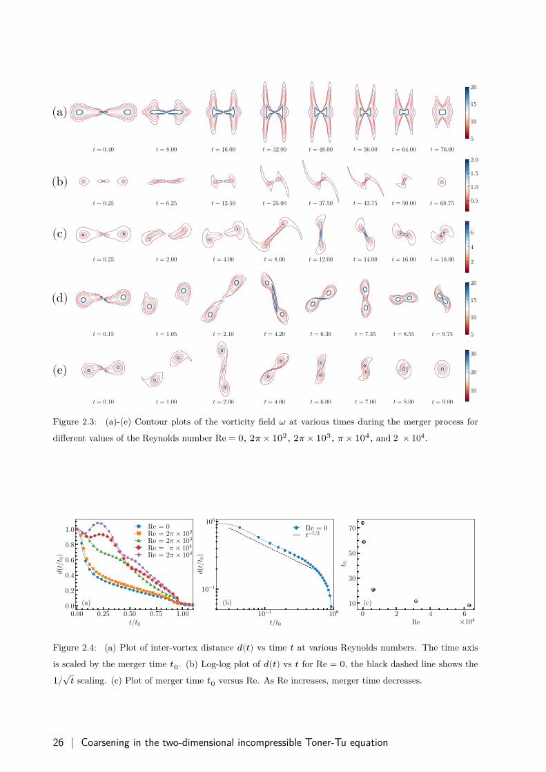
Figure 2.3: (a)-(e) Contour plots of the vorticity field 𝜔 at various times during the merger process for
different values of the Reynolds number Re = 0, 2𝜋 × 102, 2𝜋 × 103, 𝜋 × 104, and 2� × 104.
0.00 0.25 0.50 0.75 1.00t/t0
0.0
0.2
0.4
0.6
0.8
1.0
d(t/t
0)
(a)
Re = 0Re = 2π × 102
Re = 2π × 103
Re = π × 104
Re = 2π × 104
10−1 100
t/t0
10−1
100
d(t/t
0)
(b)
Re = 0t−1/2
0 2 4 6Re ×104
10
30
50
70
t 0
(c)
Figure 2.4: (a) Plot of inter-vortex distance 𝑑(𝑡) vs time 𝑡 at various Reynolds numbers. The time axis
is scaled by the merger time 𝑡0. (b) Log-log plot of 𝑑(𝑡) vs 𝑡 for Re = 0, the black dashed line shows the
1/√
𝑡 scaling. (c) Plot of merger time 𝑡0 versus Re. As Re increases, merger time decreases.
26 | Coarsening in the two-dimensional incompressible Toner-Tu equation
2.7 Energy dissipation rate and energy spectrum
To further quantify coarsening dynamics, we conduct a series of high-resolution DNS (𝑁 =2048) of the ITT equation by varying Re while keeping Cn = 1/(100𝐿) fixed. For en-
semble averaging, we evolve 48 independent realizations at every Re. We monitor the
evolution of the energy spectrum 𝐸𝑘(𝑡) ≡ 12 ∑𝑘−1/2≤𝑞<𝑘+1/2⟨|��𝐪(𝑡)|2⟩ and the energy
dissipation rate (or equivalently the excess free energy) 𝜖(𝑡) ≡ ⟨2𝜈 ∑𝑘 𝑘2𝐸𝑘(𝑡)⟩. Here
��𝐤(𝑡) ≡ ∑𝐱 𝐮(𝐱, 𝑡) exp(−𝑖𝐤 ⋅ 𝐱), 𝑖 =√
−1, and the angular brackets indicate ensemble
average 4.
2.7.1 Energy dissipation rate
Figure 2.5: (a) Plot of the energy dissipation rate 𝜖(𝑡) vs time at various Reynolds numbers. The early
time evolution of 𝜖(𝑡) is well approximated by (2.8) (solid black line). At late times, 𝜖(𝑡) decays as
𝜖(𝑡) ∼ 𝑡−𝛿 ln(𝑡) (black solid lines) with 𝛿 obtained using a least-squares fit. (b) Plot of Re vs 𝛿 and the fit
𝛿 ∼ 1 + 0.46 ln(Re/Re∗) at higher Re. Re∗ = 3.16 × 10³ is marked by a vertical black dashed line. For
Re → 0, consistent with Ginzburg-Landau scaling, we obtain 𝛿 → 1.
The time evolution of the energy dissipation rate 𝜖(𝑡) is shown in Fig. 2.5(a). For the
initial disordered configuration, because the statistics of velocity separation is Gaussian, we
approximate the fourth-order correlations in terms of product of second-order correlations
to get the following equation for the early time evolution of the energy spectrum [47]
𝜕𝑡𝐸𝑘(𝑡) ≈ [2𝛼 − 8𝛽𝐸(𝑡)]𝐸𝑘(𝑡) − 2𝜈𝑘2𝐸𝑘(𝑡), (2.8)
where 𝐸(𝑡) = ∑𝑘 𝐸𝑘(𝑡). In Fig. 2.5 we show that the early-time evolution of the energy
dissipation rate 𝜖(𝑡) obtained from (2.8) is in good agreement with the DNS.4The energy spectrum 𝐸𝑘 and the structure factor 𝑆𝑘 are related to each other as 𝐸𝑘 = 𝑘𝑑−1𝑆𝑘.
Energy dissipation rate and energy spectrum | 27
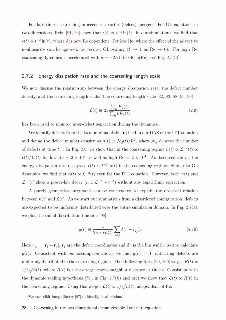
For late times, coarsening proceeds via vortex (defect) mergers. For GL equations in
two dimensions, Refs. [91, 94] show that 𝜖(𝑡) ∝ 𝑡−1 ln(𝑡). In our simulations, we find that
𝜖(𝑡) ∝ 𝑡−𝛿 ln(𝑡), where 𝛿 is now Re dependent. For low Re, where the effect of the advective
nonlinearity can be ignored, we recover GL scaling (𝛿 → 1 as Re → 0). For high Re,
coarsening dynamics is accelerated with 𝛿 = −2.71 + 0.46 ln(Re) [see Fig. 2.5(b)].
2.7.2 Energy dissipation rate and the coarsening length scale
We now discuss the relationship between the energy dissipation rate, the defect number
density, and the coarsening length scale. The coarsening length scale [82, 83, 88, 95, 96]
L(𝑡) ≡ 2𝜋 ∑𝑘 𝐸𝑘(𝑡)∑𝑘 𝑘𝐸𝑘(𝑡) (2.9)
has been used to monitor inter-defect separation during the dynamics.
We identify defects from the local minima of the |𝐮| field in our DNS of the ITT equation
and define the defect number density as 𝑛(𝑡) ≡ N𝑑(𝑡)/𝐿2, where N𝑑 denotes the number
of defects at time 𝑡 5. In Fig. 2.6, we show that in the coarsening regime 𝑛(𝑡) ∝ L−2(𝑡) ∝𝜖(𝑡)/ ln(𝑡) for low Re = 2 × 10² as well as high Re = 2 × 10⁴. As discussed above, the
energy dissipation rate decays as 𝜖(𝑡) ∼ 𝑡−𝛿 ln(𝑡) in the coarsening regime. Similar to GL
dynamics, we find that 𝑛(𝑡) ∝ L−2(𝑡) even for the ITT equation. However, both 𝑛(𝑡) and
L−2(𝑡) show a power-law decay (𝑛 ∝ L−2 ∼ 𝑡−𝛿) without any logarithmic correction.
A purely geometrical argument can be constructed to explain the observed relation
between 𝑛(𝑡) and L(𝑡). As we start our simulations from a disordered configuration, defects
are expected to be uniformly distributed over the entire simulation domain. In Fig. 2.7(a),
we plot the radial distribution function [98]
𝑔(𝑟) ≡ 12𝜋𝑟d𝑟𝑛(𝑡) ∑
𝑖≠𝑗𝛿(𝑟 − 𝑟𝑖𝑗). (2.10)
Here 𝑟𝑖𝑗 = |𝐫𝑖 − 𝐫𝑗|, 𝐫𝑖 are the defect coordinates and d𝑟 is the bin width used to calculate
𝑔(𝑟). Consistent with our assumption above, we find 𝑔(𝑟) = 1, indicating defects are
uniformly distributed in the coarsening regime. Then following Refs. [99, 100] we get 𝑅(𝑡) =1/2√𝑛(𝑡), where 𝑅(𝑡) is the average nearest-neighbor distance at time 𝑡. Consistent with
the dynamic scaling hypothesis [79], in Fig. 2.7(b) and 4(c) we show that L(𝑡) ∝ 𝑅(𝑡) in
the coarsening regime. Using this we get L(𝑡) ∝ 1/√𝑛(𝑡) independent of Re.
5We use scikit-image library [97] to identify local minima
28 | Coarsening in the two-dimensional incompressible Toner-Tu equation
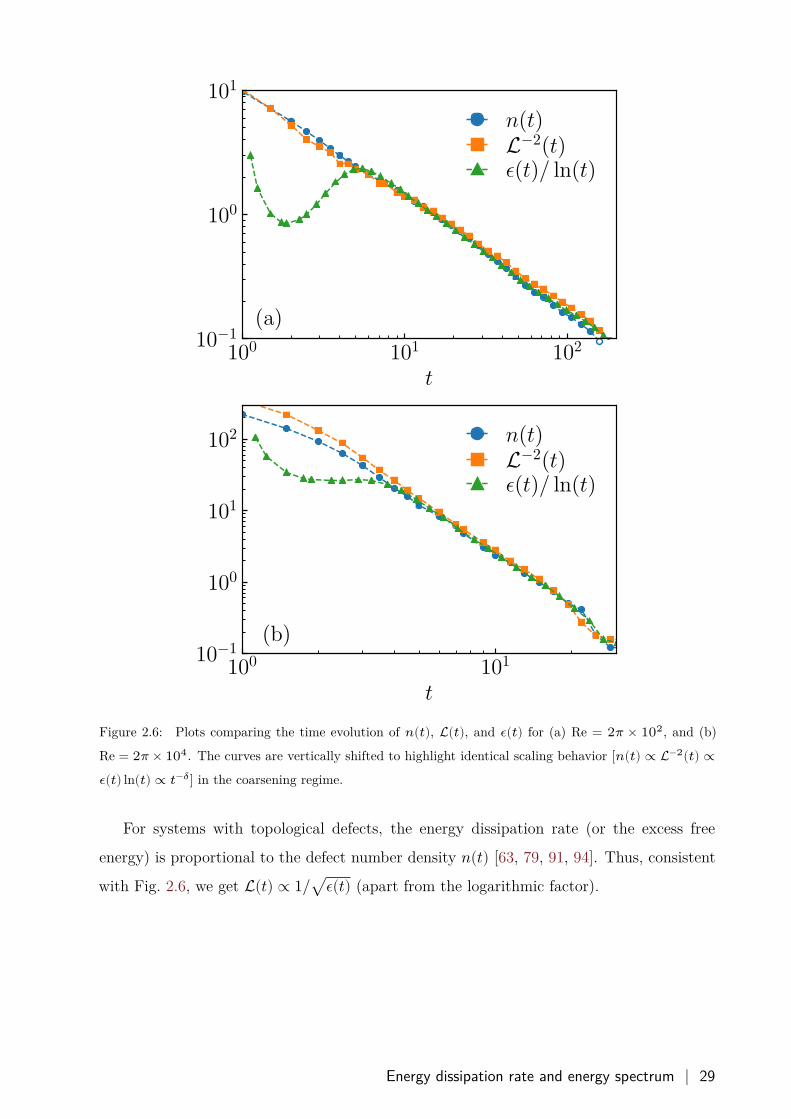
Figure 2.6: Plots comparing the time evolution of 𝑛(𝑡), L(𝑡), and 𝜖(𝑡) for (a) Re = 2𝜋 × 102, and (b)
Re = 2𝜋 × 104. The curves are vertically shifted to highlight identical scaling behavior [𝑛(𝑡) ∝ L−2(𝑡) ∝𝜖(𝑡) ln(𝑡) ∝ 𝑡−𝛿] in the coarsening regime.
For systems with topological defects, the energy dissipation rate (or the excess free
energy) is proportional to the defect number density 𝑛(𝑡) [63, 79, 91, 94]. Thus, consistent
with Fig. 2.6, we get L(𝑡) ∝ 1/√𝜖(𝑡) (apart from the logarithmic factor).
Energy dissipation rate and energy spectrum | 29
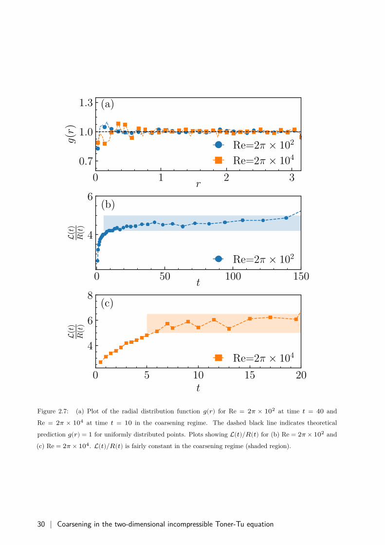
Figure 2.7: (a) Plot of the radial distribution function 𝑔(𝑟) for Re = 2𝜋 × 102 at time 𝑡 = 40 and
Re = 2𝜋 × 104 at time 𝑡 = 10 in the coarsening regime. The dashed black line indicates theoretical
prediction 𝑔(𝑟) = 1 for uniformly distributed points. Plots showing L(𝑡)/𝑅(𝑡) for (b) Re = 2𝜋 × 102 and
(c) Re = 2𝜋 × 104. L(𝑡)/𝑅(𝑡) is fairly constant in the coarsening regime (shaded region).
30 | Coarsening in the two-dimensional incompressible Toner-Tu equation
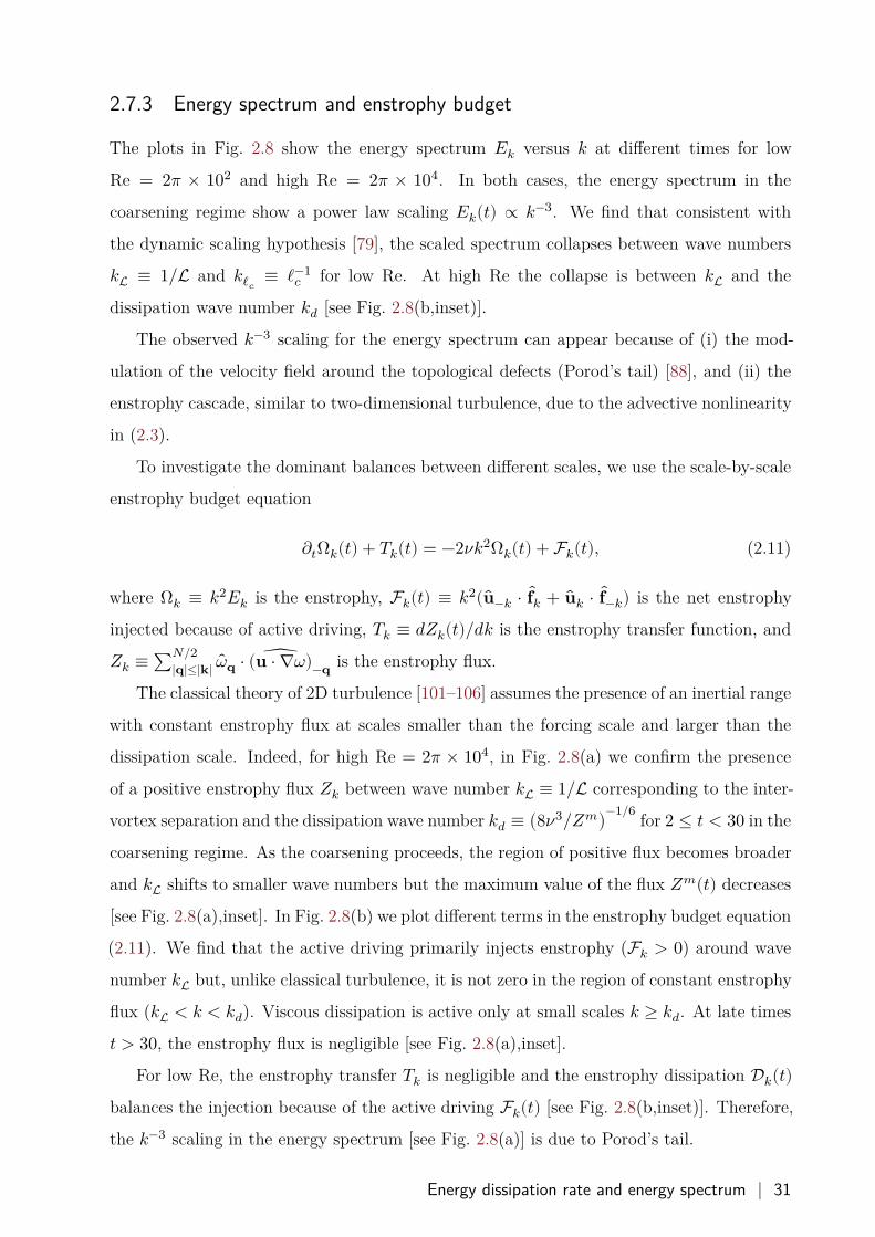
2.7.3 Energy spectrum and enstrophy budget
The plots in Fig. 2.8 show the energy spectrum 𝐸𝑘 versus 𝑘 at different times for low
Re = 2𝜋 × 102 and high Re = 2𝜋 × 104. In both cases, the energy spectrum in the
coarsening regime show a power law scaling 𝐸𝑘(𝑡) ∝ 𝑘−3. We find that consistent with
the dynamic scaling hypothesis [79], the scaled spectrum collapses between wave numbers
𝑘L ≡ 1/L and 𝑘ℓ𝑐≡ ℓ−1
𝑐 for low Re. At high Re the collapse is between 𝑘L and the
dissipation wave number 𝑘𝑑 [see Fig. 2.8(b,inset)].
The observed 𝑘−3 scaling for the energy spectrum can appear because of (i) the mod-
ulation of the velocity field around the topological defects (Porod’s tail) [88], and (ii) the
enstrophy cascade, similar to two-dimensional turbulence, due to the advective nonlinearity
in (2.3).
To investigate the dominant balances between different scales, we use the scale-by-scale
enstrophy budget equation
𝜕𝑡Ω𝑘(𝑡) + 𝑇𝑘(𝑡) = −2𝜈𝑘2Ω𝑘(𝑡) + F𝑘(𝑡), (2.11)
where Ω𝑘 ≡ 𝑘2𝐸𝑘 is the enstrophy, F𝑘(𝑡) ≡ 𝑘2(��−𝑘 ⋅ 𝐟𝑘 + ��𝑘 ⋅ 𝐟−𝑘) is the net enstrophy
injected because of active driving, 𝑇𝑘 ≡ 𝑑𝑍𝑘(𝑡)/𝑑𝑘 is the enstrophy transfer function, and
𝑍𝑘 ≡ ∑𝑁/2|𝐪|≤|𝐤| ��𝐪 ⋅ (𝐮 ⋅ ∇𝜔)−𝐪 is the enstrophy flux.
The classical theory of 2D turbulence [101–106] assumes the presence of an inertial range
with constant enstrophy flux at scales smaller than the forcing scale and larger than the
dissipation scale. Indeed, for high Re = 2𝜋 × 104, in Fig. 2.8(a) we confirm the presence
of a positive enstrophy flux 𝑍𝑘 between wave number 𝑘L ≡ 1/L corresponding to the inter-
vortex separation and the dissipation wave number 𝑘𝑑 ≡ (8𝜈3/𝑍𝑚)−1/6 for 2 ≤ 𝑡 < 30 in the
coarsening regime. As the coarsening proceeds, the region of positive flux becomes broader
and 𝑘L shifts to smaller wave numbers but the maximum value of the flux 𝑍𝑚(𝑡) decreases
[see Fig. 2.8(a),inset]. In Fig. 2.8(b) we plot different terms in the enstrophy budget equation
(2.11). We find that the active driving primarily injects enstrophy (F𝑘 > 0) around wave
number 𝑘L but, unlike classical turbulence, it is not zero in the region of constant enstrophy
flux (𝑘L < 𝑘 < 𝑘𝑑). Viscous dissipation is active only at small scales 𝑘 ≥ 𝑘𝑑. At late times
𝑡 > 30, the enstrophy flux is negligible [see Fig. 2.8(a),inset].
For low Re, the enstrophy transfer 𝑇𝑘 is negligible and the enstrophy dissipation D𝑘(𝑡)balances the injection because of the active driving F𝑘(𝑡) [see Fig. 2.8(b,inset)]. Therefore,
the 𝑘−3 scaling in the energy spectrum [see Fig. 2.8(a)] is due to Porod’s tail.
Energy dissipation rate and energy spectrum | 31
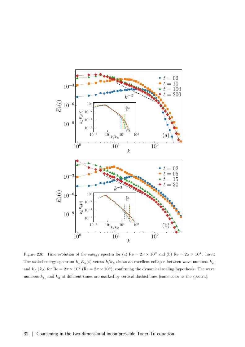
Figure 2.8: Time evolution of the energy spectra for (a) Re = 2𝜋 × 102 and (b) Re = 2𝜋 × 104. Inset:
The scaled energy spectrum 𝑘L𝐸𝑘(𝑡) versus 𝑘/𝑘L shows an excellent collapse between wave numbers 𝑘L
and 𝑘ℓ𝑐(𝑘𝑑) for Re = 2𝜋 × 102 (Re = 2𝜋 × 104), confirming the dynamical scaling hypothesis. The wave
numbers 𝑘ℓ𝑐and 𝑘𝑑 at different times are marked by vertical dashed lines (same color as the spectra).
32 | Coarsening in the two-dimensional incompressible Toner-Tu equation
Figure 2.9: (a) Plot of the enstrophy flux 𝑍𝑘(𝑡)/𝑍𝑚(𝑡) versus 𝑘 at Re = 2𝜋×104 for different times in the
coarsening regime. Wave numbers 𝑘L and 𝑘𝑑 are marked with vertical dashed lines (same color as the main
plot). Inset: Time evolution of 𝑍𝑚(𝑡). (b) Enstrophy budget: Plot of the transfer function T𝑘 ≡ 𝑑𝑍𝑘/𝑑𝑘,
enstrophy injection due to the active driving F𝑘, and the enstrophy dissipation D𝑘 = −2𝜈𝑘2Ω𝑘 for
Re = 2𝜋 × 104 and at time 𝑡 = 7 in the coarsening regime. Inset: Plot of different terms in the enstrophy
budget for low Re = 2𝜋 × 102 and at time 𝑡 = 25 in the coarsening regime.
Energy dissipation rate and energy spectrum | 33
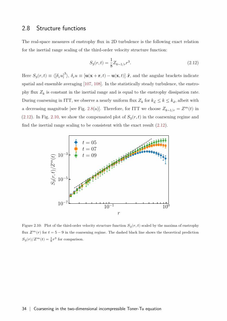
2.8 Structure functions
The real-space measures of enstrophy flux in 2D turbulence is the following exact relation
for the inertial range scaling of the third-order velocity structure function:
𝑆3(𝑟, 𝑡) = 18𝑍𝑘∼1/𝑟𝑟3. (2.12)
Here 𝑆3(𝑟, 𝑡) ≡ ⟨[𝛿𝑟𝑢]3⟩, 𝛿𝑟𝑢 ≡ [𝐮(𝐱 + 𝐫, 𝑡) − 𝐮(𝐱, 𝑡)] . 𝐫, and the angular brackets indicate
spatial and ensemble averaging [107, 108]. In the statistically steady turbulence, the enstro-
phy flux 𝑍𝑘 is constant in the inertial range and is equal to the enstrophy dissipation rate.
During coarsening in ITT, we observe a nearly uniform flux 𝑍𝑘 for 𝑘L ≤ 𝑘 ≤ 𝑘𝑑, albeit with
a decreasing magnitude [see Fig. 2.8(a)]. Therefore, for ITT we choose 𝑍𝑘∼1/𝑟 = 𝑍𝑚(𝑡) in
(2.12). In Fig. 2.10, we show the compensated plot of 𝑆3(𝑟, 𝑡) in the coarsening regime and
find the inertial range scaling to be consistent with the exact result (2.12).
10−1 100
r
10−7
10−5
10−3
S3(r,t
)/Zm
(t)
t = 05t = 07t = 09
Figure 2.10: Plot of the third-order velocity structure function 𝑆3(𝑟, 𝑡) scaled by the maxima of enstrophy
flux 𝑍𝑚(𝑟) for 𝑡 = 5 − 9 in the coarsening regime. The dashed black line shows the theoretical prediction
𝑆3(𝑟)/𝑍𝑚(𝑡) = 18 𝑟3 for comparison.
34 | Coarsening in the two-dimensional incompressible Toner-Tu equation
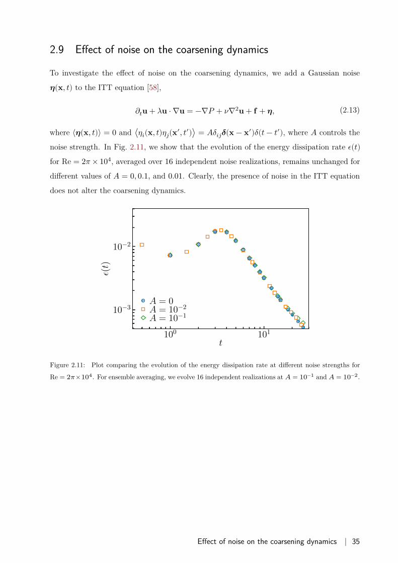
2.9 Effect of noise on the coarsening dynamics
To investigate the effect of noise on the coarsening dynamics, we add a Gaussian noise
𝜼(𝐱, 𝑡) to the ITT equation [58],
𝜕𝑡𝐮 + 𝜆𝐮 ⋅ ∇𝐮 = −∇𝑃 + 𝜈∇2𝐮 + 𝐟 + 𝜼, (2.13)
where ⟨𝜼(𝐱, 𝑡)⟩ = 0 and ⟨𝜂𝑖(𝐱, 𝑡)𝜂𝑗(𝐱′, 𝑡′)⟩ = 𝐴𝛿𝑖𝑗𝜹(𝐱 − 𝐱′)𝛿(𝑡 − 𝑡′), where 𝐴 controls the
noise strength. In Fig. 2.11, we show that the evolution of the energy dissipation rate 𝜖(𝑡)for Re = 2𝜋 × 104, averaged over 16 independent noise realizations, remains unchanged for
different values of 𝐴 = 0, 0.1, and 0.01. Clearly, the presence of noise in the ITT equation
does not alter the coarsening dynamics.
100 101
t
10−3
10−2
ε(t)
A = 0A = 10−2
A = 10−1
Figure 2.11: Plot comparing the evolution of the energy dissipation rate at different noise strengths for
Re = 2𝜋×104. For ensemble averaging, we evolve 16 independent realizations at 𝐴 = 10−1 and 𝐴 = 10−2.
Effect of noise on the coarsening dynamics | 35
2.10 Coarsening in ITT versus bacterial turbulence
Bacterial turbulence (BT) refers to the chaotic spatio-temporal flows generated by dense
suspensions of motile bacteria [8, 10]. The dynamics of a turbulent bacterial suspension is
modeled by the ITT equation, albeit with the viscous dissipation in ITT replaced with a
Swift-Hohenberg-type fourth-order term to mimic energy injection due to bacterial swim-
ming [10, 47, 109–111],
𝜕𝑡𝐮 + 𝜆𝐮 ⋅ ∇𝐮 = −∇𝑃 − 𝜈∇2𝐮 − Γ∇4𝐮 + 𝐟, (2.14)
where 𝜈 > 0 and the parameter Γ > 0.
In contrast to BT (2.14) , the ITT is a model of flocking dynamics. Indeed the ho-
mogeneous, ordered state is a stable solution of the ITT (2.3) but not of BT (2.14). Fur-
thermore, (2.14) and its variants show an inverse energy transfer from small scales to large
scales, whereas during coarsening in ITT we observe a forward enstrophy cascade from the
coarsening length scale L to small scales.
2.11 Pseudo-spectral algorithm for the 2D ITT equation
In this section, we describe the numerical methods used for the direct numerical simulations
(DNS) of the ITT equation(2.3). We use a pseudo-spectral method in the stream function-
vorticity formulation [86, 87] to perform DNS of (2.3) in a periodic square box of side
length 𝐿, and discretize the simulation domain with 𝑁2 collocation points. Unless stated
otherwise, we set 𝐿 = 2𝜋 and 𝑁 = 2048. The stream function-vorticity formulation of the
ITT equation reads as
𝜕𝑡𝝎 + 𝜆𝐮 ⋅ ∇𝝎 = 𝜈∇2𝝎 + 𝛼𝝎 − 𝛽∇ × (|𝐮|2𝐮). (2.15)
Here 𝝎 ≡ 𝑧 ⋅ ∇ × 𝐮 is the vorticity field, 𝐮 = (𝜕𝑦𝜓, −𝜕𝑥𝜓), and 𝜓 satisfies the Laplace
equation 𝜔 = ∇2𝜓. In Fourier space, (2.15) is
𝜕𝑡𝝎 + 𝜆 (𝐮 ⋅ ∇𝝎) = (𝛼 − 𝜈𝑘2) 𝝎 − 𝛽𝐤 × (|𝐮|2𝐮), (2.16)
where 𝝎(𝐤, 𝑡) ≡ ∑𝐱 𝝎(𝐱, 𝑡) exp(−𝑖𝐤 ⋅ 𝐱) is the Fourier transform of the vorticity field. We
discretize time with steps of size Δ𝑡 and use a second-order exponential time differencing
scheme (ETD2)[112] for time integration.
36 | Coarsening in the two-dimensional incompressible Toner-Tu equation
ETD schemes integrate the −𝜈𝑘2𝝎 term explicitly, and the other terms are approximated
by their weighted sum at the time steps 𝑛 and 𝑛 − 1. The ETD2 discretized form of (2.16)
is
𝝎(𝐤, 𝑡 + Δ𝑡) = 𝝎(𝐤, 𝑡)𝑒𝑐Δ𝑡 + (1 + 𝑐Δ𝑡)𝑒𝑐Δ𝑡 − 1 − 2𝑐Δ𝑡Δ𝑡𝑐2 𝐹(𝐤, 𝑡) + 1 + 𝑐Δ𝑡 − 𝑒𝑐Δ𝑡
Δ𝑡𝑐2 𝐹(𝐤, 𝑡 − Δ𝑡).(2.17)
Here 𝑐 = −𝜈𝑘2 and 𝐹(𝐤, 𝑡) = 𝜆𝐮 ⋅ ∇𝝎 − 𝛽(𝐤 × |𝐮|2𝐮). Since 𝐹(𝐤, 𝑡 − Δ𝑡) is not known at
𝑡 = 0, we integrate (2.16) at the first time step using an ETD1 scheme
𝝎(𝐤, 𝑡 + Δ𝑡) = 𝝎(𝐤, 𝑡)𝑒𝑐Δ𝑡 + 𝑒𝑐Δ𝑡 − 1𝑐 𝐹(𝐤, 𝑡). (2.18)
In the limit 𝑐 = 0, for example for 𝑘 = 0, ETD1 scheme reduces to the Euler scheme and
ETD2 scheme reduces to the Adam-Bashford scheme.
The mean vorticity in the simulation domain is zero; ⟨𝜔⟩ = ⟨𝜕𝑥𝑢𝑦 − 𝜕𝑦𝑢𝑥⟩ = 06, as a
result 𝐮 computed from the stream function only contains the fluctuating part of the local
velocity, and the mean velocity 𝐮 in the stream function-vorticity formulation is also zero.
To account for the global long-range order that may arise during the evolution, we evolve
the mean velocity separately. We integrate (2.3) over the entire simulation domain, to get
the equation of motion for the mean velocity
𝜕𝑡𝐮 = 𝛼𝐮 − 𝛽|𝐮|2𝐮. (2.19)
𝐮 is then updated using (2.19) and added to the fluctuating 𝐮 computed from the stream
function in real space before computing 𝐮 ⋅ ∇𝝎 at each time step. In Algorithm. 1, we
outline our numerical algorithm.
6⟨𝜕𝑓/𝜕𝑥𝑖⟩ = 0 for any periodic function 𝑓.
Pseudo-spectral algorithm for the 2D ITT equation | 37
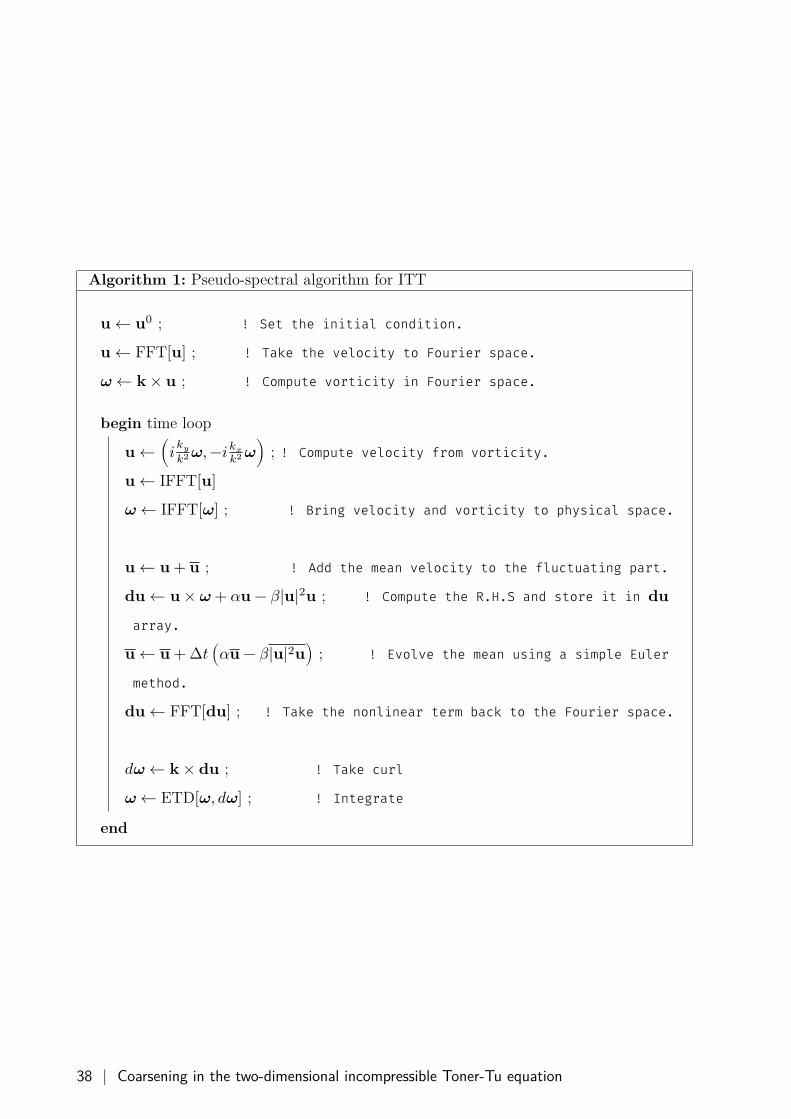
Algorithm 1: Pseudo-spectral algorithm for ITT
𝐮 ← 𝐮0 ; ! Set the initial condition.
𝐮 ← FFT[𝐮] ; ! Take the velocity to Fourier space.
𝝎 ← 𝐤 × 𝐮 ; ! Compute vorticity in Fourier space.
begin time loop
𝐮 ← (𝑖𝑘𝑦𝑘2 𝝎, −𝑖𝑘𝑥
𝑘2 𝝎) ; ! Compute velocity from vorticity.
𝐮 ← IFFT[𝐮]𝝎 ← IFFT[𝝎] ; ! Bring velocity and vorticity to physical space.
𝐮 ← 𝐮 + 𝐮 ; ! Add the mean velocity to the fluctuating part.
𝐝𝐮 ← 𝐮 × 𝝎 + 𝛼𝐮 − 𝛽|𝐮|2𝐮 ; ! Compute the R.H.S and store it in 𝐝𝐮array.
𝐮 ← 𝐮 + Δ𝑡 (𝛼𝐮 − 𝛽|𝐮|2𝐮) ; ! Evolve the mean using a simple Euler
method.
𝐝𝐮 ← FFT[𝐝𝐮] ; ! Take the nonlinear term back to the Fourier space.
𝑑𝝎 ← 𝐤 × 𝐝𝐮 ; ! Take curl
𝝎 ← ETD[𝝎, 𝑑𝝎] ; ! Integrate
end
38 | Coarsening in the two-dimensional incompressible Toner-Tu equation
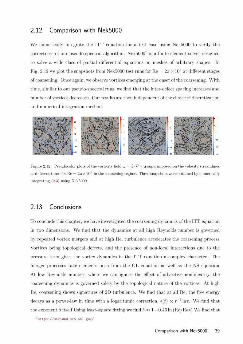
2.12 Comparison with Nek5000
We numerically integrate the ITT equation for a test case using Nek5000 to verify the
correctness of our pseudo-spectral algorithm. Nek50007 is a finite element solver designed
to solve a wide class of partial differential equations on meshes of arbitrary shapes. In
Fig. 2.12 we plot the snapshots from Nek5000 test runs for Re = 2𝜋×104 at different stages
of coarsening. Once again, we observe vortices emerging at the onset of the coarsening. With
time, similar to our pseudo-spectral runs, we find that the inter-defect spacing increases and
number of vortices decreases. Our results are then independent of the choice of discretization
and numerical integration method.
Figure 2.12: Pseudocolor plots of the vorticity field 𝜔 = 𝑧 ⋅∇×𝐮 superimposed on the velocity streamlines
at different times for Re = 2𝜋×104 in the coarsening regime. These snapshots were obtained by numerically
integrating (2.3) using Nek5000.
2.13 Conclusions
To conclude this chapter, we have investigated the coarsening dynamics of the ITT equation
in two dimensions. We find that the dynamics at all high Reynolds number is governed
by repeated vortex mergers and at high Re, turbulence accelerates the coarsening process.
Vortices being topological defects, and the presence of non-local interactions due to the
pressure term gives the vortex dynamics in the ITT equation a complex character. The
merger processes take elements both from the GL equation as well as the NS equation.
At low Reynolds number, where we can ignore the effect of advective nonlinearity, the
coarsening dynamics is governed solely by the topological nature of the vortices. At high
Re, coarsening shows signatures of 2D turbulence. We find that at all Re, the free energy
decays as a power-law in time with a logarithmic correction, 𝜖(𝑡) ∝ 𝑡−𝛿 ln 𝑡. We find that
the exponent 𝛿 itself Using least-square fitting we find 𝛿 ≈ 1+0.46 ln (Re/Re∗) We find that7https://nek5000.mcs.anl.gov/
Comparison with Nek5000 | 39
the exponent 𝛿 itself is an increasing function of Re. As Re → 0, 𝛿 → 1, and we recover the
GL scaling. We find that at all Re, the energy spectrum shows a power-law scaling of 𝑘−3.
At low Re, the scaling appears due to the Porod’s law. At high Re, we show the presence
of a forward enstrophy cascade, which extends the power law scaling to much higher wave
numbers as compared to low Re. Finally, we verify the exact relation for the third-order
velocity structure-function at high Re.
40 | Coarsening in the two-dimensional incompressible Toner-Tu equation
Chapter 3
Phase ordering, defects, and turbulence in the3D incompressible Toner-Tu equation
We investigate coarsening dynamics of the incompressible Toner-Tu equation in three di-
mensions. We show that the dynamics is characterized by Reynolds number Re. At all
Re, coarsening proceeds via defect merger events. At low Re, the dynamics is similar to
the Ginzburg-Landau equation. We find a unique growing length scale viz. the inter-defect
spacing and dynamical scaling holds. At high Re, turbulence alters the coarsening dynam-
ics. In particular, we observe a forward energy cascade and multi-scaling similar to classical
three-dimensional turbulence.
3.1 Introduction
Phase ordering (or coarsening) refers to the dynamics of a system from a disordered state
to an orientationally ordered phase with broken symmetry on a sudden change of the con-
trol parameter [63, 113]. Biological systems such as a fish school or a flock of birds show
collective behavior - an otherwise randomly moving group of organisms start to perform co-
herent motion to generate spectacularly ordered patterns whose size is much larger than an
individual organism [2, 18, 73]. Although the exact biological or environmental factors that
trigger such transition depend on the particular species, physicists have successfully used
the theory of dry-active matter to study disorder-order phase transition in these systems
[4, 34, 114]. Theoretical studies have revealed that for an incompressible or a Malthu-
sian flock, where we can ignore density fluctuations, the order-disorder phase transition is
continuous [58, 60–62].
| 41
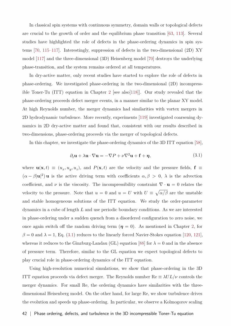
In classical spin systems with continuous symmetry, domain walls or topological defects
are crucial to the growth of order and the equilibrium phase transition [63, 113]. Several
studies have highlighted the role of defects in the phase-ordering dynamics in spin sys-
tems [70, 115–117]. Interestingly, suppression of defects in the two-dimensional (2D) XY
model [117] and the three-dimensional (3D) Heisenberg model [70] destroys the underlying
phase-transition, and the system remains ordered at all temperatures.
In dry-active matter, only recent studies have started to explore the role of defects in
phase-ordering. We investigated phase-ordering in the two-dimensional (2D) incompress-
ible Toner-Tu (ITT) equation in Chapter 2 [see also[118]]. Our study revealed that the
phase-ordering proceeds defect merger events, in a manner similar to the planar XY model.
At high Reynolds number, the merger dynamics had similarities with vortex mergers in
2D hydrodynamic turbulence. More recently, experiments [119] investigated coarsening dy-
namics in 2D dry-active matter and found that, consistent with our results described in
two-dimensions, phase-ordering proceeds via the merger of topological defects.
In this chapter, we investigate the phase-ordering dynamics of the 3D ITT equation [58],
𝜕𝑡𝐮 + 𝜆𝐮 ⋅ ∇𝐮 = −∇𝑃 + 𝜈∇2𝐮 + 𝐟 + 𝜼, (3.1)
where 𝐮(𝐱, 𝑡) ≡ (𝑢𝑥, 𝑢𝑦, 𝑢𝑧), and 𝑃(𝐱, 𝑡) are the velocity and the pressure fields, 𝐟 ≡(𝛼 − 𝛽|𝐮|2) 𝐮 is the active driving term with coefficients 𝛼, 𝛽 > 0, 𝜆 is the advection
coefficient, and 𝜈 is the viscosity. The incompressibility constraint ∇ ⋅ 𝐮 = 0 relates the
velocity to the pressure. Note that 𝑢 = 0 and 𝑢 = 𝑈 with 𝑈 ≡ √𝛼/𝛽 are the unstable
and stable homogeneous solutions of the ITT equation. We study the order-parameter
dynamics in a cube of length 𝐿 and use periodic boundary conditions. As we are interested
in phase-ordering under a sudden quench from a disordered configuration to zero noise, we
once again switch off the random driving term (𝜼 = 0). As mentioned in Chapter 2, for
𝛽 = 0 and 𝜆 = 1, Eq. (3.1) reduces to the linearly forced Navier-Stokes equation [120, 121],
whereas it reduces to the Ginzburg-Landau (GL) equation [88] for 𝜆 = 0 and in the absence
of pressure term. Therefore, similar to the GL equation we expect topological defects to
play crucial role in phase-ordering dynamics of the ITT equation.
Using high-resolution numerical simulations, we show that phase-ordering in the 3D
ITT equation proceeds via defect merger. The Reynolds number Re ≡ 𝜆𝑈𝐿/𝜈 controls the
merger dynamics. For small Re, the ordering dynamics have similarities with the three-
dimensional Heisenberg model. On the other hand, for large Re, we show turbulence drives
the evolution and speeds up phase-ordering. In particular, we observe a Kolmogorov scaling
42 | Phase ordering, defects, and turbulence in the 3D incompressible Toner-Tu equation
in the energy spectrum over a range of length scales, and a detailed analysis of the velocity
structure-functions reveals multi-fractal scaling.
The rest of the chapter is organised as follows. In Section 3.2 we discuss the details
of our direct numerical simulations. In Section 3.3 we present the results for the mean
order and the energy dissipation rate at low and high Re. In Sections 3.4.1 and 3.4.2 we
characterize the coarsening at low and high Re respectively. We conclude the chapter in
Section 3.5.
3.2 Direct numerical simulations
The dimensionless form of the ITT equation is [see Chapter 2 and [118]]:
𝜕𝑡𝐮 + ReCn2𝐮 ⋅ ∇𝐮 = −∇𝑃 + Cn2∇2𝐮 + (1 − |𝐮|2) 𝐮, (3.2)
where Re ≡ 𝜆𝑈𝐿/𝜈 is the Reynolds number with 𝑈 ≡ √𝛼/𝛽, and Cn = √𝜈/𝛼𝐿2 is the
Cahn number.
We use a pseudospectral method to perform direct numerical simulation (DNS) of
Eq. (3.2) in a tri-periodic cubic box of length 𝐿 = 2𝜋. We discretize the box with 𝑁3 collo-
cation points with 𝑁 = 1024 and use a second-order exponential time differencing scheme
for time integration [112]. We decompose the velocity field into its mean 𝐕(𝑡) = ⟨𝐮⟩ and
fluctuating part 𝐮′(𝑥, 𝑡) ≡ 𝐮(𝑥, 𝑡) − 𝐕(𝑡) to investigate the ordering dynamics, where the
angular brackets denote spatial averaging. Along with the velocity field, we monitor the
evolution of the energy spectrum
𝐸𝑘(𝑡) ≡ 12 ∑
𝑘− 12 ≤𝑝<𝑘+ 1
2
|��𝐩(𝑡)|2, (3.3)
and the energy E(𝑡) = ∑𝑁/2𝑘=1 𝐸𝑘(𝑡). Here, ��𝐤(𝑡) ≡ ∑𝐱 𝐮(𝐱, 𝑡) exp(−𝑖𝐤 ⋅ 𝐱) is the Fourier
transform of the velocity field with 𝑖 =√
−1 [118]. Note that the total energy is 𝐸(𝑡) ≡∑𝑁/2
𝑘=0 𝐸𝑘(𝑡)12𝑉 2(𝑡) + E(𝑡). The flow is initialized with a disordered configuration with
𝐸𝑘(𝑡 = 0) = 𝐴𝑘2 and 𝐴 = 10−8. In our DNS, we choose Cn = 1/(2𝜋 × 102), 𝑈 = 1, and
vary Re.
Direct numerical simulations | 43
20 40 60 80 100t
10−4
10−3
10−2
10−1
100
V(t
)
(a)
10−1 100
t
10−4
10−2
V(t
)
et
Re=0Re=2π × 102
Re=5π × 103
Re= π × 104
Re=2π × 104
20 40 60 80t
0.1
0.2
0.3
0.4
0.5
E(t)
(b)
10−1 100
t
10−3
10−1
E(t)
t−32 e2t
Re=0Re=2π × 102
Re=5π × 103
Re= π × 104
Re=2π × 104
Figure 3.1: Time evolution of (a) the mean velocity 𝑉 (𝑡) and (b) the fluctuating energy E(𝑡) for different
Re. (Insets) Zoomed in plots compare early time-evolution with the corresponding theoretical prediction
(dashed black lines).
3.3 Results
3.3.1 Average velocity
In Fig. 3.1, we plot the magnitude of the mean velocity 𝑉 (𝑡) and the fluctuation energy
E(𝑡) = ∑𝑁/2𝑘=1 𝐸𝑘(𝑡). At early times, the nonlinearities in Eq. (3.1) can be ignored and we
44 | Phase ordering, defects, and turbulence in the 3D incompressible Toner-Tu equation
arrive at the following time evolution equation of the energy spectrum [47, 118]
𝜕𝑡𝐸𝑘(𝑡) ≈ 2(1 − Cn2𝑘2)𝐸𝑘(𝑡). (3.4)
Using Eq. (3.4) and the initial condition for the energy spectrum we obtain 𝑉 (𝑡) ∼ exp(𝑡)and E ∼ exp(2𝑡)/𝑡3/2 [see Fig. 3.1]. The departure from the early exponential growth of 𝑉 (𝑡)and E(𝑡) marks the onset of the phase-ordering regime. We observe that 𝑉 (𝑡) approaches
the ordered state faster by increasing the Reynolds number. On the other hand, E(𝑡) first
increases, attains a plateau and then decreases. The plateau region and the peak value of
E(𝑡) decrease with increasing Reynolds. We show later in Section 3.4.2 that the shorter
plateau region is an indicator of strength of the forward energy cascade.
3.3.2 Excess free energy surfaces and topological defects
For the ITT equations, the excess free-energy per unit volume is ℎ ≡ Cn2|∇𝐮|2/2 and
the defects are identified as velocity nulls, i.e. spatial locations where 𝐮 = 𝟎. For a 𝑛-
component order parameter in 𝐷-dimensions, the dimensionality of the defects is 𝑛 − 𝐷[63]. Since 𝑛 = 𝐷 = 3 for us, the ITT equation permits unit magnitude topological
charge. We locate defects using the algorithm prescribed by Berg and Lüscher [69] that
has been successfully used to study: (a) the role of defects in the 3D Heisenberg transition
[70], and (b) coarsening dynamics in the 3D Ginzburg-Landau equations [116]. Similar
algorithms have also been used to identify vector nulls in magnetohydrodynamics [122, 123]
and homogeneous, isotropic turbulence [124].
In Fig. 3.2(a,b) we show the time evolution of the iso-ℎ surfaces overlaid with defect
positions during phase-ordering for low and high-Re. The streamline plots of pair of oppo-
sitely charged defects undergoing merger are shown in Fig. 3.2(c) [Re = 0] and Fig. 3.2(d)
[Re = 2𝜋 × 104]. At low Re, in Fig. 3.2(a), we show that the iso-surfaces are primar-
ily localized around the lines joining oppositely charged defects. The evolution resembles
phase-ordering in the 3D Ginzburg-Landau equations [115, 116]; we shall explore this fur-
ther in Section 3.4. In contrast, at high-Re we observe tubular structures similar to fluid
turbulence [125] and the defects reside in the proximity of these tubes [see Fig. 3.2(b)].
Results | 45
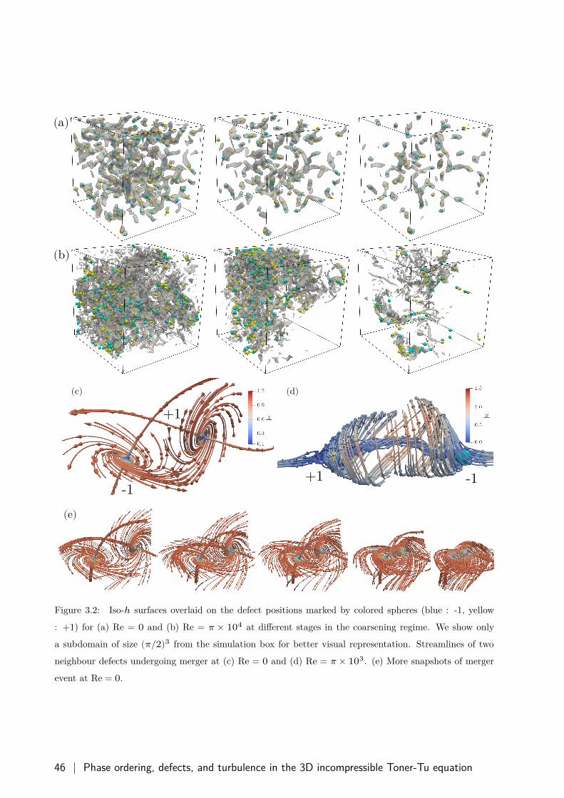
Figure 3.2: Iso-ℎ surfaces overlaid on the defect positions marked by colored spheres (blue : -1, yellow
: +1) for (a) Re = 0 and (b) Re = 𝜋 × 104 at different stages in the coarsening regime. We show only
a subdomain of size (𝜋/2)3 from the simulation box for better visual representation. Streamlines of two
neighbour defects undergoing merger at (c) Re = 0 and (d) Re = 𝜋 × 103. (e) More snapshots of merger
event at Re = 0.
46 | Phase ordering, defects, and turbulence in the 3D incompressible Toner-Tu equation
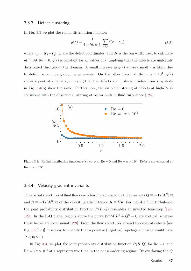
3.3.3 Defect clustering
In Fig. 3.3 we plot the radial distribution function
𝑔(𝑟) ≡ 14𝜋𝑟2𝑑𝑟𝑛(𝑡) ∑
𝑖≠𝑗𝛿(𝑟 − 𝑟𝑖𝑗), (3.5)
where 𝑟𝑖𝑗 = |𝐫𝑖 −𝐫𝑗|, 𝐫𝑖 are the defect coordinates, and 𝑑𝑟 is the bin width used to calculate
𝑔(𝑟). At Re = 0, 𝑔(𝑟) is constant for all values of 𝑟, implying that the defects are uniformly
distributed throughout the domain. A small increase in 𝑔(𝑟) at very small 𝑟 is likely due
to defect pairs undergoing merger events. On the other hand, at Re = 𝜋 × 104, 𝑔(𝑟)shows a peak at smaller 𝑟, implying that the defects are clustered. Indeed, our snapshots
in Fig. 3.4(b) show the same. Furthermore, the visible clustering of defects at high-Re is
consistent with the observed clustering of vector nulls in fluid turbulence [124].
0.5 1.0 1.5 2.0r
0
5
10
g(r
)
(a) Re = 0Re = π × 104
Figure 3.3: Radial distribution function 𝑔(𝑟) vs. 𝑟 at Re = 0 and Re = 𝜋 × 104. Defects are clustered at
Re = 𝜋 × 104.
3.3.4 Velocity gradient invariants
The spatial structures of fluid flows are often characterized by the invariants 𝑄 ≡ −Tr(𝐀2)/3and 𝑅 ≡ −Tr(𝐀3)/3 of the velocity gradient tensor 𝐀 ≡ ∇𝐮. For high-Re fluid turbulence,
the joint probability distribution function 𝑃(𝑅, 𝑄) resembles an inverted tear-drop [126–
129]. In the R-Q plane, regions above the curve (27/4)𝑅2 + 𝑄3 = 0 are vortical, whereas
those below are extensional [129]. From the flow structures around topological defects [see
Fig. 3.2(c,d)], it is easy to identify that a positive (negative) topological charge would have
𝑅 < 0(> 0).In Fig. 3.4, we plot the joint probability distribution function 𝑃(𝑅, 𝑄) for Re = 0 and
Re = 2𝜋 × 104 at a representative time in the phase-ordering regime. By overlaying the 𝑄
Results | 47
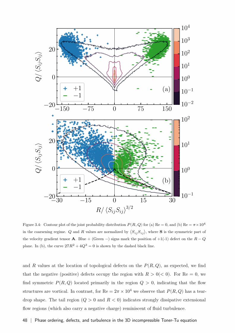
−150 −75 0 75 150−20
0
20
Q/〈S
ijSij〉
(a)+1−1
−30 −15 0 15 30
R/ 〈SijSij〉3/2−20
0
20
Q/〈S
ijSij〉
(b)+1−1
10−2
10−1
100
101
102
103
104
10−1
100
101
102
Figure 3.4: Contour plot of the joint probability distribution 𝑃(𝑅, 𝑄) for (a) Re = 0, and (b) Re = 𝜋×104
in the coarsening regime. 𝑄 and 𝑅 values are normalized by ⟨𝑆𝑖𝑗𝑆𝑖𝑗⟩, where 𝐒 is the symmetric part of
the velocity gradient tensor 𝐀. Blue + (Green −) signs mark the position of +1(-1) defect on the 𝑅 − 𝑄plane. In (b), the curve 27𝑅2 + 4𝑄3 = 0 is shown by the dashed black line.
and 𝑅 values at the location of topological defects on the 𝑃(𝑅, 𝑄), as expected, we find
that the negative (positive) defects occupy the region with 𝑅 > 0(< 0). For Re = 0, we
find symmetric 𝑃 (𝑅, 𝑄) located primarily in the region 𝑄 > 0, indicating that the flow
structures are vortical. In contrast, for Re = 2𝜋 × 104 we observe that 𝑃(𝑅, 𝑄) has a tear-
drop shape. The tail region (𝑄 > 0 and 𝑅 < 0) indicates strongly dissipative extensional
flow regions (which also carry a negative charge) reminiscent of fluid turbulence.
48 | Phase ordering, defects, and turbulence in the 3D incompressible Toner-Tu equation
3.4 Energy spectrum and the phase ordering length scale
A unique length scale typically describes the dynamics of systems undergoing phase-ordering,
this is often referred to as the dynamic scaling hypothesis. In Chapter 2 we have shown
that at all Re, there exists a unique growing length scale, namely the inter-defect separa-
tion, that determines the coarsening dynamics. In the following sections we investigate the
validity of this hypothesis for phase-ordering in the 3D ITT equation for low and high-Re.
3.4.1 Low Reynolds number
In Fig. 3.5, we plot the energy spectrum. With time, the peak of the spectrum shifts towards
small-wave numbers, indicating a growing length scale often defined as [88, 88, 91, 94, 113,
118, 130]
L(𝑡) ≡ 2𝜋 ∑𝑘 𝐸𝑘(𝑡)∑𝑘 𝑘𝐸𝑘(𝑡) . (3.6)
For low Re → 0, consistent with the Ginzburg-Landau scaling, we observe L(𝑡) ∼√
𝑡 [see
Fig. 3.5(b)] [79]. The rescaled energy spectrum 𝑘L𝐸𝑘 versus 𝑘/𝑘L collapses onto a single
curve for different times [see Fig. 3.5(a)], and we observe Porod’s scaling 𝐸𝑘L ∝ (𝑘L)−4
for 𝑘L(𝑡) > 1 due to the presence of defects [79]. Note that the energy spectrum and the
structure factor are related to each other as 𝐸(𝑘, 𝑡) = 4𝜋𝑘2𝑆(𝑘, 𝑡).
Dynamical scaling hypothesis
The plot in Fig. 3.5(b) shows that the average minimum inter-defect separation 𝑅(𝑡) ∝ L(𝑡),validating the dynamical scaling hypothesis. For uniformly distributed defects, we expect
L(𝑡) ∝ 𝑛(𝑡)−1/3, where 𝑛(𝑡) is the defect number density [99, 100, 118]. We verify the same
in Fig. 3.5(b,inset).
Energy spectrum and the phase ordering length scale | 49
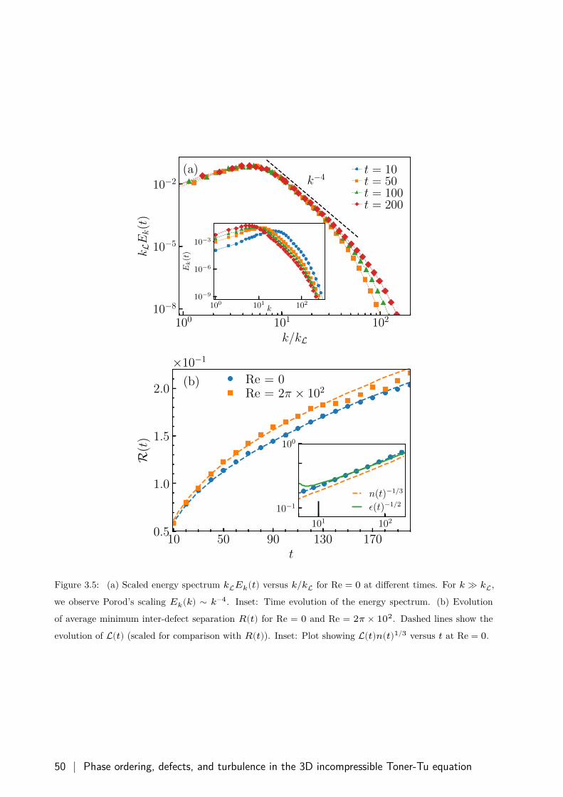
100 101 102
k/kL
10−8
10−5
10−2
kLE
k(t
)
k−4(a)
100 101 102k
10−9
10−6
10−3
Ek(t
)
t = 10t = 50t = 100t = 200
10 50 90 130 170t
0.5
1.0
1.5
2.0
R(t)
×10−1
(b)
101 102
10−1
100
n(t)−1/3
ε(t)−1/2
Re = 0Re = 2π × 102
Figure 3.5: (a) Scaled energy spectrum 𝑘L𝐸𝑘(𝑡) versus 𝑘/𝑘L for Re = 0 at different times. For 𝑘 ≫ 𝑘L,
we observe Porod’s scaling 𝐸𝑘(𝑘) ∼ 𝑘−4. Inset: Time evolution of the energy spectrum. (b) Evolution
of average minimum inter-defect separation 𝑅(𝑡) for Re = 0 and Re = 2𝜋 × 102. Dashed lines show the
evolution of L(𝑡) (scaled for comparison with 𝑅(𝑡)). Inset: Plot showing L(𝑡)𝑛(𝑡)1/3 versus 𝑡 at Re = 0.
50 | Phase ordering, defects, and turbulence in the 3D incompressible Toner-Tu equation
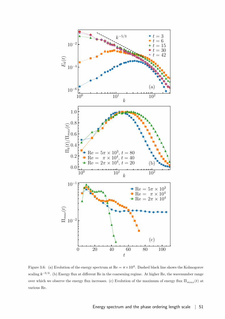
100 101 102
k
10−6
10−4
10−2
Ek(t
)
k−5/3
(a)
t = 3t = 6t = 15t = 30t = 42
100 101 102
k
0.0
0.2
0.4
0.6
0.8
1.0
Πk(t
)/Πmax(t
)
(b)
Re = 5π × 103, t = 80Re = π × 104, t = 40Re = 2π × 104, t = 20
0 20 40 60 80 100t
10−2
10−1
Πmax(t
)
(c)
Re = 5π × 103
Re = π × 104
Re = 2π × 104
Figure 3.6: (a) Evolution of the energy spectrum at Re = 𝜋×104. Dashed black line shows the Kolmogorov
scaling 𝑘−5/3. (b) Energy flux at different Re in the coarsening regime. At higher Re, the wavenumber range
over which we observe the energy flux increases. (c) Evolution of the maximum of energy flux Π𝑚𝑎𝑥(𝑡) at
various Re.
Energy spectrum and the phase ordering length scale | 51
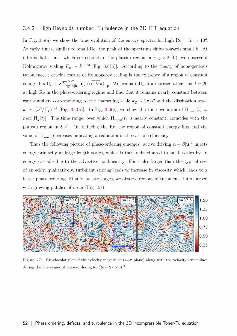
3.4.2 High Reynolds number: Turbulence in the 3D ITT equation
In Fig. 3.6(a) we show the time evolution of the energy spectra for high Re = 5𝜋 × 103.
At early times, similar to small Re, the peak of the spectrum shifts towards small 𝑘. At
intermediate times which correspond to the plateau region in Fig. 3.2 (b), we observe a
Kolmogorov scaling 𝐸𝑘 ∼ 𝑘−5/3 [Fig. 3.6(b)]. According to the theory of homogeneous
turbulence, a crucial feature of Kolmogorov scaling is the existence of a region of constant
energy flux Π𝑘 ≡ 𝜆 ∑𝑁/2|𝐩|≤|𝐤| ��𝐩 ⋅ (𝐮 ⋅ ∇𝐮)−𝐩. We evaluate Π𝑘 at a representative time 𝑡 = 20
at high Re in the phase-ordering regime and find that it remains nearly constant between
wave-numbers corresponding to the coarsening scale 𝑘L ∼ 2𝜋/L and the dissipation scale
𝑘𝜂 ∼ (𝜈3/Π𝑘)1/4 [Fig. 3.6(b)]. In Fig. 3.6(c), we show the time evolution of Π𝑚𝑎𝑥(𝑡) ≡𝑚𝑎𝑥[Π𝑘(𝑡)]. The time range, over which Π𝑚𝑎𝑥(𝑡) is nearly constant, coincides with the
plateau region in E(𝑡). On reducing the Re, the region of constant energy flux and the
value of Π𝑚𝑎𝑥 decreases indicating a reduction in the cascade efficiency.
Thus the following picture of phase-ordering emerges: active driving 𝛼 − 𝛽|𝐮|2 injects
energy primarily at large length scales, which is then redistributed to small scales by an
energy cascade due to the advective nonlinearity. For scales larger than the typical size
of an eddy, qualitatively, turbulent stirring leads to increase in viscosity which leads to a
faster phase-ordering. Finally, at late stages, we observe regions of turbulence interspersed
with growing patches of order (Fig. 3.7).
Figure 3.7: Pseudocolor plot of the velocity magnitude (z=𝜋 plane) along with the velocity streamlines
during the late stages of phase-ordering for Re = 2𝜋 × 104.
52 | Phase ordering, defects, and turbulence in the 3D incompressible Toner-Tu equation
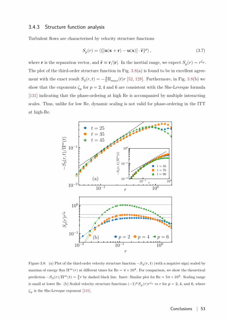
3.4.3 Structure function analysis
Turbulent flows are characterised by velocity structure functions
𝑆𝑝(𝑟) = ⟨{[𝐮(𝐱 + 𝐫) − 𝐮(𝐱)] ⋅ 𝐫}𝑝⟩ , (3.7)
where 𝐫 is the separation vector, and 𝐫 ≡ 𝐫/|𝐫|. In the inertial range, we expect 𝑆𝑝(𝑟) ∼ 𝑟𝜁𝑝 .
The plot of the third-order structure function in Fig. 3.8(a) is found to be in excellent agree-
ment with the exact result 𝑆3(𝑟, 𝑡) = −45Π𝑚𝑎𝑥(𝑡)𝑟 [52, 128]. Furthermore, in Fig. 3.8(b) we
show that the exponents 𝜁𝑝 for 𝑝 = 2, 4 and 6 are consistent with the She-Leveque formula
[131] indicating that the phase-ordering at high Re is accompanied by multiple interacting
scales. Thus, unlike for low Re, dynamic scaling is not valid for phase-ordering in the ITT
at high-Re.
10−1 100r
10−2
10−1
−S3(r,t
)/Πm
(t)
(a)10−1 100
r10−2
10−1
100
−S3(r,t
)/Πm
(t)
t = 50t = 70t = 90
t = 25t = 35t = 45
10−2 10−1 100
r
10−1
100
Sp(r
)rζ p
(b) p = 2 p = 4 p = 6
Figure 3.8: (a) Plot of the third-order velocity structure function −𝑆3(𝑟, 𝑡) (with a negative sign) scaled by
maxima of energy flux Π𝑚(𝑟) at different times for Re = 𝜋×104. For comparison, we show the theoretical
prediction −𝑆3(𝑟)/Π𝑚(𝑡) = 45 𝑟 by dashed black line. Inset: Similar plot for Re = 5𝜋×103. Scaling range
is small at lower Re. (b) Scaled velocity structure functions (−1)𝑝𝑆𝑝(𝑟)𝑟𝜁𝑝 vs 𝑟 for 𝑝 = 2, 4, and 6, where
𝜁𝑝 is the She-Leveque exponent [131].
Conclusions | 53
3.5 Conclusions
In this chapter, we have studied the phase-ordering dynamics of the 3D ITT equation. We
found that similar to 2D, coarsening proceeds via repeated defect merger. At low Re, the
defects are uniformly distributed throughout the domain and the coarsening dynamics is
characterized by a unique growing length scale. On the other hand, at high Re, defects
are clustered and the advective nonlinearities alter the coarsening dynamics. We find that
transient states enroute to global order show characteristics of three-dimensional turbulence.
In particular, we observe a near constant energy flux in the coarsening regime, with the
turbulent showing multi-fractal intermittent nature.
54 | Phase ordering, defects, and turbulence in the 3D incompressible Toner-Tu equation
Chapter 4
Dense suspensions of polar active particles
In this chapter, we study dense, wet suspensions of active polar particles in two and three
dimensions. We first investigate the instabilities of the aligned state to small perturbations
and show how inertia can stabilize the orientational order. Further, we perform high resolu-
tion direct numerical simulations and characterize the nature of the turbulent states arising
in such systems.
4.1 Introduction
Self-propelled particles in a bulk fluid display a variety of dynamical phenomenon, from
chaotic flows to ordered collective motion [2, 8, 10, 18, 49, 51, 132, 133]. Of particular
interest to us are suspensions of polar active particles.
At low Reynolds number, viscous forces dominate over the inertial forces, such suspen-
sions are well described by Stokesian hydrodynamics, where the inertia is ignored com-
pletely. For example, the typical size of an Escherichia coli bacterium is around 5𝜇𝑚 and
it swims at an average speed of 10𝜇𝑚/𝑠, which sets the Reynolds number on its scale at
Re ∼ 10−5 − 10−4 [10, 46]. Bacterial suspensions are then overwhelmingly Stokesian. In
this limit, Simha and Ramaswamy [29] have shown that orientationally ordered states of
swimmers are unstable to small perturbations. The instability arises as follows: A perfectly
aligned state of active swimmers in quiescent fluid results in uniform uni axial stress. Per-
turbations on this state generate spatially varying stresses, which give rise to a net local
fluid flow. The resulting flow alters the alignment of the swimmers and can amplify the
perturbations, destabilizing the orientational order. Suspensions of extensile (contractile)
swimmers are unstable to bend (splay) perturbations [see Fig. 1.4 in Chapter 1] .
| 55
Simha-Ramaswamy instability at low Re results in lively chaotic flows widely observed
in bacterial suspensions [8, 10]. The phenomenon is also known as active turbulence or meso-
scale turbulence [see [10] and Fig. 1.1 in Chapter 1]. These chaotic flows are characterized
by the absence of global orientational order; instead, coherent structures (vortices) with
size much larger than a single individual but smaller than the experimental domain are
observed [8–10, 47–51].
Activity is not limited to low Re swimmers and aligned swimmers moving collectively
are frequently observed in bulk fluid in regimes that are far away from the Stokesian limit.
Clearly these swimmers are successful in escaping the Stokesian instability which governs
the fate of low Re swimmers. We can group these flocks into two categories: (a) Flocks of
swimmers where Re at an individual’s scale is very large (Re ≫ 1), such as sardine schools.
In this case, inertial forces are orders of magnitude larger than the viscous forces and hence
inviscid hydrodynamic interactions alone determine the dynamics of such flocks [18, 134].
(b) Flocks of swimmers with Re ∼ O(1), like brine shrimp, larval squids, fish schools where
individuals of size O(𝑚𝑚) are found moving at a speed O(𝑚𝑚𝑠−1) [134] in water. For such
swimmers inertial and viscous forces are comparable to each other and play an essential
role in determining the dynamics.
In this chapter, we consider the latter type of swimmers, and ask the following ques-
tion: Can inertia stabilize the ordered state in extensile suspensions against the Stokesian
instability? We focus on dense suspensions, where fluctuations in active particle concentra-
tion are small compared to its average value and are ignored [58]. This situation arises in
various experimental systems like dense bacterial suspensions with short-ranged repulsive
interactions [10, 47], in microfluidic experiments with self-propelled colloids [59], and in
systems with long-ranged repulsive interactions like bird flocks [58, 60] where the density is
maintained at an optimal level.
We show that indeed, inertia can stabilize the ordered state with respect to small
perturbations. Our linear stability analysis reveals that a single dimensionless parame-
ter 𝑅 ≡ 𝜌𝑣20/2𝜎0, where 𝜌 is the suspension mass density, 𝑣0 is the self-propulsion speed of
active particles, and 𝜎0 is the force-dipole density, governs the stability of the suspension to
small perturbations. For 𝑅 < 𝑅1, where 𝑅1 = 1 + 𝜆 and 𝜆 is the flow-alignment parameter,
we find an inviscid instability where the most unstable pure bend modes grow at a rate
I(𝜔) ∝ 𝑞. For 𝑅1 < 𝑅 < 𝑅2, we find that the pure bend perturbations grow at a rate
I(𝜔) ∝ 𝑞2. Finally for 𝑅 > 𝑅2, orientational order is stable. Our numerical studies in two
56 | Dense suspensions of polar active particles

dimensions show that the chaotic flows at all 𝑅 < 𝑅2 are riddled with topological vortices
and we do not observe any global order. Inter-defect spacing grows as we increase R and
appears to diverge at 𝑅 ∼ 𝑅2.
The rest of chapter is organized as follows. In Section 4.2 we write down the equations
of motion for dense suspensions in the constant concentration limit. In Section 4.3 we
outline our linear stability analysis results. In Section 4.5 we present the results of our
numerical simulations in two dimensions and in Section 4.7 we present the results from our
three-dimensional simulations. Finally we contrast our results for dense suspensions with
our earlier study of Malthusian suspensions [55, 135].
Introduction | 57
4.2 Equations of motion
The equations of motion for a suspension of polar self-propelled particles (SPP) described
by the hydrodynamic velocity field 𝐮(𝐱, 𝑡), the polar order parameter field 𝐩(𝐱, 𝑡), and the
concentration 𝑐(𝐱, 𝑡) are [18, 29, 45, 55, 136]
𝜌 (𝜕𝑡𝐮 + 𝐮 ⋅ ∇𝐮) = −∇𝑃 + 𝜇∇2𝐮 − ∇. (𝚺𝑎 + 𝚺𝑟) ,
𝜕𝑡𝐩 + (𝐮 + 𝑣0𝐩) ⋅ ∇𝐩 = 𝜆𝐒.𝐩 + 𝛀.𝐩 + Γ𝐡 + ℓ∇2𝐮, and
𝜕𝑡𝑐 + ∇ ⋅ [(𝐮 + 𝑣1𝐩)𝑐] = 0.
(4.1)
Here 𝜌 is the suspension density, 𝜇 is the fluid viscosity, and the hydrodynamic pressure
term 𝑃(𝐱, 𝑡) enforces incompressibility ∇ ⋅ 𝐮 = 0. 𝐒 and 𝛀 are the symmetric and anti-
symmetric parts of the velocity gradient tensor ∇𝐮, 𝜆 is the flow alignment parameter, 𝑣0𝐩is the local self-propulsion velocity of the active particles, and 𝑣1𝐩 is the velocity at which
the polar order parameter advects the concentration field.
𝚺𝑎 = 𝜎𝑎(𝑐)𝐩𝐩 + 𝛾𝑎(𝑐) (∇𝐩 + ∇𝐩𝑇 ) (4.2)
is the intrinsic stress associated with the swimming activity, where 𝜎𝑎 > 0(< 0) is the force-
dipole density for extensile (contractile) swimmers and 𝛾𝑎 determines the polar contribution
to the active stress [29, 55, 136].
𝚺𝑟 = 𝜆+𝐡𝐩 + 𝜆−𝐩𝐡 + ℓ(∇𝐡 + ∇𝐡𝑇 ) (4.3)
is the reversible thermodynamic stress [137], 𝜆± = (𝜆 ± 1)/2, and 𝐡 = −𝛿𝐹/𝛿𝐩 is the
molecular field conjugate to 𝐩, derived from a free-energy functional
𝐹 = ∫ 𝑑3𝑟 [𝐾2 (∇𝐩)2 + 1
4(𝐩.𝐩 − 1)2 − 𝐸𝐩 ⋅ ∇𝑐] (4.4)
that favors a aligned order parameter state with unit magnitude. For simplicity, we choose
a single Frank constant 𝐾, which penalizes gradients in 𝐩 [44]. 𝐸 favors the alignment of
𝐩 to up or down gradients of 𝑐, according to its sign. Γ is the rotational mobility for the
relaxation of the order parameter field, and ℓ governs the lowest-order polar flow-coupling
term [45]. All the coefficients in our hydrodynamic description are phenomenological in
nature. In particular, 𝜎𝑎(𝑐) and 𝛾𝑎(𝑐) are functions of the concentration 𝑐 and in the limit
𝑐 → 0 are proportional to 𝑐.
58 | Dense suspensions of polar active particles
4.2.1 Equations for dense suspensions
In the constant concentration limit (𝑐 = 𝑐0), number conservation implies the incompress-
ibility constraint on the order parameter ∇ ⋅ 𝐩 = 0 [58]. Further, all the phenomenological
parameters take their values at 𝑐0. In our earlier study on Malthusian flocks [55] we have
shown that 𝛾𝑎 and ℓ do not alter the nature of the inviscid instability and only change
the coefficients of O(𝑞2) terms in the dispersion relation. In coming sections, we will show
that only splay-bend modes couple to the number-conservation. Twist-bend modes are de-
termined solely by the 𝐮 and 𝐩 dynamics. Thus, the nature of instability of these modes
is identical for number conserving, Malthusian, and dense suspensions. 𝛾𝑎 and ℓ will then
have similar effects in the constant concentration limit as well and we set them to zero to
simplify our analysis. Our effective equations of motion then are
𝜌 (𝜕𝑡𝐮 + 𝐮.∇𝐮) = −∇𝑃 + 𝜇∇2𝐮 − 𝜎0𝐩 ⋅ ∇𝐩 − ∇ ⋅ (𝜆−𝐩𝐡 + 𝜆+𝐡𝐩) ,
𝜕𝑡𝐩 + (𝐮 + 𝑣0𝐩).∇𝐩 = −∇Π + 𝜆𝐒.𝐩 + 𝛀.𝐩 + Γ𝐡,(4.5)
where 𝐡 = 𝐾∇2𝐩 + (1 − |𝐩|2) 𝐩, 𝜎0 = 𝜎𝑎(𝑐0) and the additional pressure-like term Πenforces the incompressibility constraint ∇ ⋅ 𝐩 = 0.
Equations of motion | 59
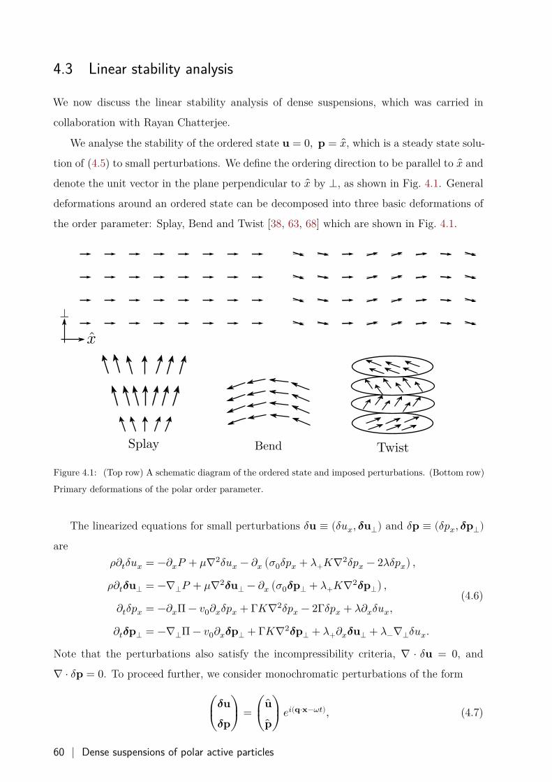
4.3 Linear stability analysis
We now discuss the linear stability analysis of dense suspensions, which was carried in
collaboration with Rayan Chatterjee.
We analyse the stability of the ordered state 𝐮 = 0, 𝐩 = 𝑥, which is a steady state solu-
tion of (4.5) to small perturbations. We define the ordering direction to be parallel to 𝑥 and
denote the unit vector in the plane perpendicular to 𝑥 by ⟂, as shown in Fig. 4.1. General
deformations around an ordered state can be decomposed into three basic deformations of
the order parameter: Splay, Bend and Twist [38, 63, 68] which are shown in Fig. 4.1.
Figure 4.1: (Top row) A schematic diagram of the ordered state and imposed perturbations. (Bottom row)
Primary deformations of the polar order parameter.
The linearized equations for small perturbations 𝛿𝐮 ≡ (𝛿𝑢𝑥, 𝜹𝐮⟂) and 𝛿𝐩 ≡ (𝛿𝑝𝑥, 𝜹𝐩⟂)are
𝜌𝜕𝑡𝛿𝑢𝑥 = −𝜕𝑥𝑃 + 𝜇∇2𝛿𝑢𝑥 − 𝜕𝑥 (𝜎0𝛿𝑝𝑥 + 𝜆+𝐾∇2𝛿𝑝𝑥 − 2𝜆𝛿𝑝𝑥) ,
𝜌𝜕𝑡𝜹𝐮⟂ = −∇⟂𝑃 + 𝜇∇2𝜹𝐮⟂ − 𝜕𝑥 (𝜎0𝜹𝐩⟂ + 𝜆+𝐾∇2𝜹𝐩⟂) ,
𝜕𝑡𝛿𝑝𝑥 = −𝜕𝑥Π − 𝑣0𝜕𝑥𝛿𝑝𝑥 + Γ𝐾∇2𝛿𝑝𝑥 − 2Γ𝛿𝑝𝑥 + 𝜆𝜕𝑥𝛿𝑢𝑥,
𝜕𝑡𝜹𝐩⟂ = −∇⟂Π − 𝑣0𝜕𝑥𝜹𝐩⟂ + Γ𝐾∇2𝜹𝐩⟂ + 𝜆+𝜕𝑥𝜹𝐮⟂ + 𝜆−∇⟂𝛿𝑢𝑥.
(4.6)
Note that the perturbations also satisfy the incompressibility criteria, ∇ ⋅ 𝛿𝐮 = 0, and
∇ ⋅ 𝛿𝐩 = 0. To proceed further, we consider monochromatic perturbations of the form
⎛⎜⎝
𝜹𝐮𝜹𝐩
⎞⎟⎠
= ⎛⎜⎝
����
⎞⎟⎠
𝑒𝑖(𝐪⋅𝐱−𝜔𝑡), (4.7)
60 | Dense suspensions of polar active particles
where 𝐪 ≡ (𝑞𝑥 𝑥 + 𝐪⟂⋅ ⟂) is the perturbation wavevector and 𝜔 = R(𝜔) + 𝑖I(𝜔), and
R(𝜔) and I(𝜔) are the real and imaginary parts of 𝜔. Ordered state will be unstable to
perturbations if I(𝜔) > 0. Substituting (4.7) in (4.6) gives
(−𝑖𝜌𝜔 + 𝜈𝑞2) ��𝑥 = −𝑖𝑞𝑥𝑃 − 𝑖(𝜎0 − 𝜆+𝐾𝑞2 − 2𝜆)𝑞𝑥 𝑝𝑥
(−𝑖𝜌𝜔 + 𝜈𝑞2) ��⟂ = −𝑖𝐪⟂𝑃 − 𝑖(𝜎0 − 𝜆+𝐾𝑞2)𝑞𝑥��⟂
(−𝑖𝜔 + Γ𝐾𝑞2 + 𝑖𝑣0𝑞𝑥) 𝑝𝑥 = −𝑖𝑞𝑥Π − 2Γ 𝑝𝑥 + 𝑖𝜆𝑞𝑥��𝑥
(−𝑖𝜔 + Γ𝐾𝑞2 + 𝑖𝑣0𝑞𝑥) ��⟂ = −𝑖𝐪⟂Π + 𝑖(𝜆+𝑞𝑥��⟂ + 𝜆−𝐪⟂��𝑥),
(4.8)
In the 𝛿𝑝𝑥 equation, the leading order term independent of the wavevector 𝐪 is −2𝛿𝑝𝑥.
In the absence of pressure term Π, perturbations parallel to the ordering direction decay
exponentially and are rendered fast [55]. Π couples the longitudinal and transverse pertur-
bations and 𝛿𝑝𝑥 is no longer a fast variable. However, incompressibility constraints on 𝐮and 𝐩 allows us to proceed in terms of transverse perturbations only, for which we have
(−𝑖𝜌𝜔 + 𝜇𝑞2)��⟂ = 2𝑖𝜆𝑞𝑥𝐪⟂ ⋅ ��⟂
𝑞2 𝐪⟂ − 𝑖𝑞𝑥 (𝜎0 − 𝜆+𝐾𝑞2) ��⟂
(−𝑖𝜔 + Γ𝐾𝑞2 + 𝑖𝑣0𝑞𝑥)��⟂ = −2Γ𝐪⟂ ⋅ ��⟂𝑞2 𝐪⟂ + 𝑖𝜆+𝑞𝑥��⟂.
(4.9)
Out of the four eigenvectors of (4.9), two are parallel to 𝐪⟂ and represent the coupled
splay-bend modes. The other two are perpendicular to 𝐪⟂ and represent the twist-bend
modes. Twist deformations are three-dimensional and hence the twist-bend modes do not
exist for two-dimensional systems.
Twist-bend modes
Taking the cross product of (4.9) with 𝐪⟂ gives us the following dispersion relation for
twist-bend modes
⎡⎢⎣
−𝑖𝜌𝜔 + 𝜇𝑞2 𝑖𝑞 cos 𝜙(𝜎0 − 𝜆+𝐾𝑞2)−𝑖𝜆+𝑞 cos 𝜙 −𝑖𝜔 + Γ𝐾𝑞2 + 𝑖𝑣0𝑞 cos 𝜙
⎤⎥⎦
⎡⎢⎣
𝐪⟂ × ��⟂
𝐪⟂ × ��⟂
⎤⎥⎦
= 0, (4.10)
where 𝑞𝑥 = 𝑞 cos 𝜙 and 𝐪⟂ = 𝑞 sin 𝜙. From the above equation we get
2𝜔𝑡± = 𝑣0𝑞 cos 𝜙 − 𝑖𝜇+
𝜌 𝑞2 ± 1𝜌√(𝜌𝑣0𝑞 cos 𝜙 + 𝑖𝜇−𝑞2)2 − 4𝜌𝜆+𝑞2 cos2 𝜙(𝜎0 − 𝜆+𝐾𝑞2),
(4.11)
where 𝜇± = 𝜇 ± Γ𝐾𝜌. A large wavelength (small 𝑞) expansion gives
2𝜔𝑡± = 𝑣0 cos 𝜙 (1 ± √1 − 𝑅1
𝑅 ) 𝑞 + 𝑖𝜇𝜌
⎛⎜⎜⎝
± (1 − 𝛽)√1 − 𝑅1
𝑅
− (1 + 𝛽)⎞⎟⎟⎠
𝑞2, (4.12)
Linear stability analysis | 61
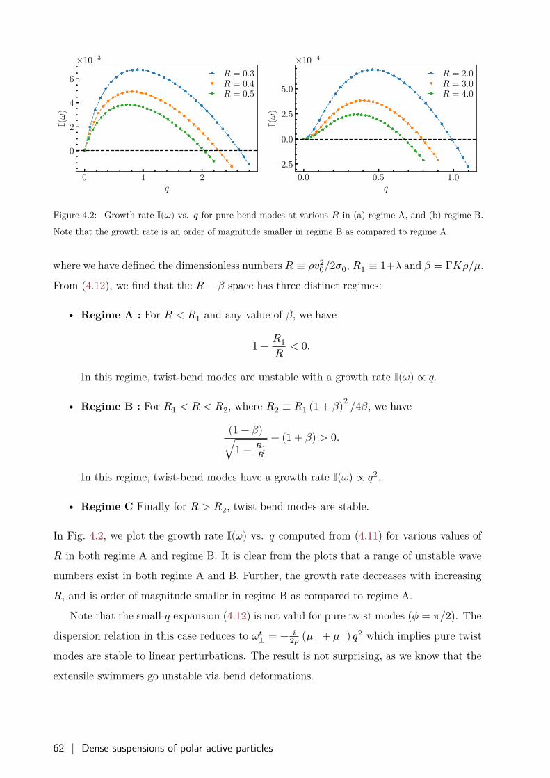
0 1 2q
0
2
4
6
I(ω
)×10−3
R = 0.3R = 0.4R = 0.5
0.0 0.5 1.0q
−2.5
0.0
2.5
5.0
I(ω
)
×10−4
R = 2.0R = 3.0R = 4.0
Figure 4.2: Growth rate I(𝜔) vs. 𝑞 for pure bend modes at various 𝑅 in (a) regime A, and (b) regime B.
Note that the growth rate is an order of magnitude smaller in regime B as compared to regime A.
where we have defined the dimensionless numbers 𝑅 ≡ 𝜌𝑣20/2𝜎0, 𝑅1 ≡ 1+𝜆 and 𝛽 = Γ𝐾𝜌/𝜇.
From (4.12), we find that the 𝑅 − 𝛽 space has three distinct regimes:
• Regime A : For 𝑅 < 𝑅1 and any value of 𝛽, we have
1 − 𝑅1𝑅 < 0.
In this regime, twist-bend modes are unstable with a growth rate I(𝜔) ∝ 𝑞.
• Regime B : For 𝑅1 < 𝑅 < 𝑅2, where 𝑅2 ≡ 𝑅1 (1 + 𝛽)2 /4𝛽, we have
(1 − 𝛽)√1 − 𝑅1
𝑅
− (1 + 𝛽) > 0.
In this regime, twist-bend modes have a growth rate I(𝜔) ∝ 𝑞2.
• Regime C Finally for 𝑅 > 𝑅2, twist bend modes are stable.
In Fig. 4.2, we plot the growth rate I(𝜔) vs. 𝑞 computed from (4.11) for various values of
𝑅 in both regime A and regime B. It is clear from the plots that a range of unstable wave
numbers exist in both regime A and B. Further, the growth rate decreases with increasing
𝑅, and is order of magnitude smaller in regime B as compared to regime A.
Note that the small-𝑞 expansion (4.12) is not valid for pure twist modes (𝜙 = 𝜋/2). The
dispersion relation in this case reduces to 𝜔𝑡± = − 𝑖
2𝜌 (𝜇+ ∓ 𝜇−) 𝑞2 which implies pure twist
modes are stable to linear perturbations. The result is not surprising, as we know that the
extensile swimmers go unstable via bend deformations.
62 | Dense suspensions of polar active particles
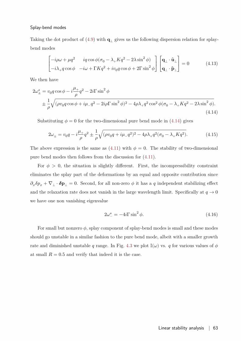
Splay-bend modes
Taking the dot product of (4.9) with 𝐪⟂ gives us the following dispersion relation for splay-
bend modes
⎡⎢⎣
−𝑖𝜌𝜔 + 𝜇𝑞2 𝑖𝑞 cos 𝜙(𝜎0 − 𝜆+𝐾𝑞2 − 2𝜆 sin2 𝜙)−𝑖𝜆+𝑞 cos 𝜙 −𝑖𝜔 + Γ𝐾𝑞2 + 𝑖𝑣0𝑞 cos 𝜙 + 2Γ sin2 𝜙
⎤⎥⎦
⎡⎢⎣
𝐪⟂ ⋅ ��⟂
𝐪⟂ ⋅ ��⟂
⎤⎥⎦
= 0 (4.13)
We then have
2𝜔𝑠± = 𝑣0𝑞 cos 𝜙 − 𝑖𝜇+
𝜌 𝑞2 − 2𝑖Γ sin2 𝜙
± 1𝜌
√(𝜌𝑣0𝑞 cos 𝜙 + 𝑖𝜇−𝑞2 − 2𝑖𝜌Γ sin2 𝜙)2 − 4𝜌𝜆+𝑞2 cos2 𝜙(𝜎0 − 𝜆+𝐾𝑞2 − 2𝜆 sin2 𝜙).(4.14)
Substituting 𝜙 = 0 for the two-dimensional pure bend mode in (4.14) gives
2𝜔± = 𝑣0𝑞 − 𝑖𝜇+𝜌 𝑞2 ± 1
𝜌√(𝜌𝑣0𝑞 + 𝑖𝜇−𝑞2)2 − 4𝜌𝜆+𝑞2(𝜎0 − 𝜆+𝐾𝑞2). (4.15)
The above expression is the same as (4.11) with 𝜙 = 0. The stability of two-dimensional
pure bend modes then follows from the discussion for (4.11).
For 𝜙 > 0, the situation is slightly different. First, the incompressibility constraint
eliminates the splay part of the deformations by an equal and opposite contribution since
𝜕𝑥𝛿𝑝𝑥 + ∇⟂ ⋅ 𝜹𝐩⟂ = 0. Second, for all non-zero 𝜙 it has a 𝑞 independent stabilizing effect
and the relaxation rate does not vanish in the large wavelength limit. Specifically at 𝑞 → 0we have one non vanishing eigenvalue
2𝜔𝑠− = −4𝑖Γ sin2 𝜙. (4.16)
For small but nonzero 𝜙, splay component of splay-bend modes is small and these modes
should go unstable in a similar fashion to the pure bend mode, albeit with a smaller growth
rate and diminished unstable 𝑞 range. In Fig. 4.3 we plot I(𝜔) vs. 𝑞 for various values of 𝜙at small 𝑅 = 0.5 and verify that indeed it is the case.
Linear stability analysis | 63
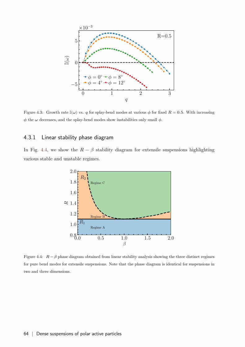
0 1 2 3q
−5
0
5
I(ω
)
×10−3
R=0.5
φ = 0◦φ = 4◦
φ = 8◦φ = 12◦
Figure 4.3: Growth rate I(𝜔) vs. 𝑞 for splay-bend modes at various 𝜙 for fixed 𝑅 = 0.5. With increasing
𝜙 the 𝜔 decreases, and the splay-bend modes show instabilities only small 𝜙.
4.3.1 Linear stability phase diagram
In Fig. 4.4, we show the 𝑅 − 𝛽 stability diagram for extensile suspensions highlighting
various stable and unstable regimes.
0.0 0.5 1.0 1.5 2.0β
0.8
1.0
1.2
1.4
1.6
1.8
2.0
R
R1
R2
Regime A
Regime B
Regime C
Figure 4.4: 𝑅 − 𝛽 phase diagram obtained from linear stability analysis showing the three distinct regimes
for pure bend modes for extensile suspensions. Note that the phase diagram is identical for suspensions in
two and three dimensions.
64 | Dense suspensions of polar active particles
4.4 Non-dimensional equations of motion
Linear stability analysis have already given us two non-dimensional numbers, 𝑅 and 𝛽which determine the stability of the ordered state [see Fig. 4.4]. By rescaling the space
𝐱′ → 𝐿𝐱, the time 𝑡′ → 𝑇 𝑡, the pressure terms 𝑃 ′ → 𝜌𝑈2𝑃 , Π′ → Π/𝑈 and the velocity
field 𝑢′𝑖 → 𝑈𝑢𝑖, where 𝑈 = 𝐿/𝑇 we get
𝜕𝑡𝑢𝑖 + 𝑢𝑗𝜕𝑗𝑢𝑖 = −𝜕𝑖𝑃 + 𝜇𝜌𝑈𝐿𝜕2
𝑗 𝑢𝑖 − 1𝜌𝑈2 𝜎0𝑝𝑗𝜕𝑗𝑝𝑖,
𝜕𝑡𝑝𝑖 + (𝑢𝑗 + 𝑣0𝑈 𝑝𝑗) 𝜕𝑗𝑝𝑖 = −𝜕𝑖Π + 𝜆−𝑝𝑗𝜕𝑖𝑢𝑗 + 𝜆+𝑝𝑗𝜕𝑗𝑢𝑖 + Γ𝐾
𝑈𝐿𝜕2𝑗 𝑝𝑖 + Γ𝐿𝑎
𝑈 (1 − 𝑝2𝑗 ) 𝑝𝑖.(4.17)
Here we have ignored the prime index for brevity. Further, choosing 𝑈 = 𝑣0 and
ℓ𝜎 = 𝜇/√𝜌𝜎0 as our velocity and length scales respectively we get
𝜕𝑡𝑢𝑖 + 𝑢𝑗𝜕𝑗𝑢𝑖 = −𝜕𝑖𝑃 + 1√𝑅𝜕2
𝑗 𝑢𝑖 − 12𝑅𝑝𝑗𝜕𝑗𝑝𝑖,
𝜕𝑡𝑝𝑖 + (𝑢𝑗 + 𝑝𝑗) 𝜕𝑗𝑝𝑖 = −𝜕𝑖Π + 𝜆−𝑝𝑗𝜕𝑖𝑢𝑗 + 𝜆+𝑝𝑗𝜕𝑗𝑢𝑖 + 𝛽√2𝑅 [𝜕2
𝑗 𝑝𝑖 + 𝜃𝛼 (1 − 𝑝2
𝑗 ) 𝑝𝑖] ,(4.18)
where we have defined the other dimensionless numbers 𝛼 = 𝐾𝜌/𝜇2, and 𝜃 = 𝑎/𝜎0.
Non-dimensional equations of motion | 65
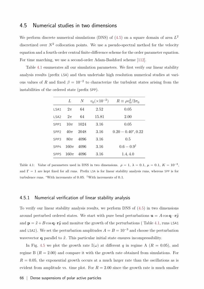
4.5 Numerical studies in two dimensions
We perform discrete numerical simulations (DNS) of (4.5) on a square domain of area 𝐿2
discretized over 𝑁2 collocation points. We use a pseudo-spectral method for the velocity
equation and a fourth-order central finite-difference scheme for the order parameter equation.
For time marching, we use a second-order Adam-Bashford scheme [112].
Table 4.1 enumerates all our simulation parameters. We first verify our linear stability
analysis results (prefix LSA) and then undertake high resolution numerical studies at vari-
ous values of 𝑅 and fixed 𝛽 = 10−2 to characterize the turbulent states arising from the
instabilities of the ordered state (prefix SPP).
𝐿 𝑁 𝑣0(×10−2) 𝑅 ≡ 𝜌𝑣20/2𝜎0
LSA1 2𝜋 64 2.52 0.05LSA2 2𝜋 64 15.81 2.00SPP1 10𝜋 1024 3.16 0.05SPP2 40𝜋 2048 3.16 0.20 − 0.40∗, 0.22SPP3 80𝜋 4096 3.16 0.5SPP4 160𝜋 4096 3.16 0.6 − 0.9†
SPP5 160𝜋 4096 3.16 1.4, 4.0
Table 4.1: Value of parameters used in DNS in two dimensions. 𝜌 = 1, 𝜆 = 0.1, 𝜇 = 0.1, 𝐾 = 10−3,
and Γ = 1 are kept fixed for all runs. Prefix LSA is for linear stability analysis runs, whereas SPP is for
turbulence runs. ∗With increments of 0.05. †With increments of 0.1.
4.5.1 Numerical verification of linear stability analysis
To verify our linear stability analysis results, we perform DNS of (4.5) in two dimensions
around perturbed ordered states. We start with pure bend perturbations 𝐮 = 𝐴 cos 𝐪 ⋅ 𝐫 𝑦and 𝐩 = 𝑥+𝐵 cos 𝐪 ⋅𝐫 𝑦 and monitor the growth of the perturbations ( Table 4.1, runs LSA1
and LSA2). We set the perturbation amplitudes 𝐴 = 𝐵 = 10−3 and choose the perturbation
wavevector 𝐪 parallel to 𝑥. This particular initial state ensures incompressibility.
In Fig. 4.5 we plot the growth rate I(𝜔) at different 𝑞 in regime A (𝑅 = 0.05), and
regime B (𝑅 = 2.00) and compare it with the growth rate obtained from simulations. For
𝑅 = 0.05, the exponential growth occurs at a much larger rate than the oscillations as is
evident from amplitude vs. time plot. For 𝑅 = 2.00 since the growth rate is much smaller
66 | Dense suspensions of polar active particles
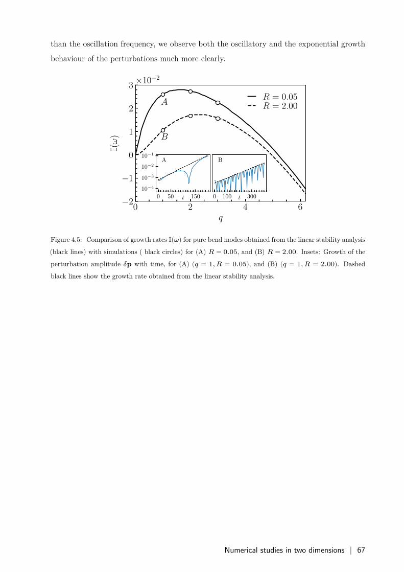
than the oscillation frequency, we observe both the oscillatory and the exponential growth
behaviour of the perturbations much more clearly.
0 2 4 6q
−2
−1
0
1
2
3
I(ω
)
×10−2
A
B
0 50 150t
10−4
10−3
10−2
10−1
A
0 100 300t
B
R = 0.05R = 2.00
Figure 4.5: Comparison of growth rates I(𝜔) for pure bend modes obtained from the linear stability analysis
(black lines) with simulations ( black circles) for (A) 𝑅 = 0.05, and (B) 𝑅 = 2.00. Insets: Growth of the
perturbation amplitude 𝛿𝐩 with time, for (A) (𝑞 = 1, 𝑅 = 0.05), and (B) (𝑞 = 1, 𝑅 = 2.00). Dashed
black lines show the growth rate obtained from the linear stability analysis.
Numerical studies in two dimensions | 67
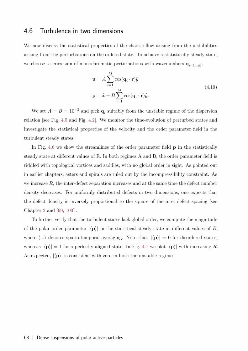
4.6 Turbulence in two dimensions
We now discuss the statistical properties of the chaotic flow arising from the instabilities
arising from the perturbations on the ordered state. To achieve a statistically steady state,
we choose a series sum of monochromatic perturbations with wavenumbers 𝐪𝑖=1…𝑀 ,
𝐮 = 𝐴𝑀
∑𝑖=1
cos(𝐪𝑖 ⋅ 𝐫) 𝑦
𝐩 = 𝑥 + 𝐵𝑀
∑𝑖=1
cos(𝐪𝑖 ⋅ 𝐫) 𝑦.(4.19)
We set 𝐴 = 𝐵 = 10−3 and pick 𝐪𝑖 suitably from the unstable regime of the dispersion
relation [see Fig. 4.5 and Fig. 4.2]. We monitor the time-evolution of perturbed states and
investigate the statistical properties of the velocity and the order parameter field in the
turbulent steady states.
In Fig. 4.6 we show the streamlines of the order parameter field 𝐩 in the statistically
steady state at different values of R. In both regimes A and B, the order parameter field is
riddled with topological vortices and saddles, with no global order in sight. As pointed out
in earlier chapters, asters and spirals are ruled out by the incompressibility constraint. As
we increase 𝑅, the inter-defect separation increases and at the same time the defect number
density decreases. For uniformly distributed defects in two dimensions, one expects that
the defect density is inversely proportional to the square of the inter-defect spacing [see
Chapter 2 and [99, 100]].
To further verify that the turbulent states lack global order, we compute the magnitude
of the polar order parameter |⟨𝐩⟩| in the statistical steady state at different values of 𝑅,
where ⟨…⟩ denotes spatio-temporal averaging. Note that, |⟨𝐩⟩| = 0 for disordered states,
whereas |⟨𝐩⟩| = 1 for a perfectly aligned state. In Fig. 4.7 we plot |⟨𝐩⟩| with increasing 𝑅.
As expected, |⟨𝐩⟩| is consistent with zero in both the unstable regimes.
68 | Dense suspensions of polar active particles
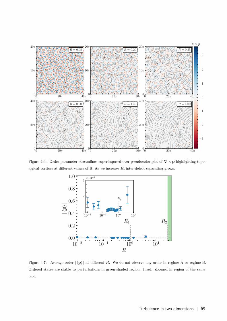
0 20π 40π0
10π
20πR = 0.05
0 20π 40π0
10π
20πR = 0.20
0 20π 40π0
10π
20πR = 0.35
0 20π 40π0
20π
40πR = 0.90
0 20π 40π0
20π
40πR = 1.40
0 20π 40π0
20π
40πR = 4.00
−3
−2
−1
0
1
2
3
∇× p
Figure 4.6: Order parameter streamlines superimposed over pseudocolor plot of ∇ × 𝐩 highlighting topo-
logical vortices at different values of R. As we increase 𝑅, inter-defect separating grows.
10−2 10−1 100 101
R
0.0
0.2
0.4
0.6
0.8
1.0
|〈p〉|
R1 R2
10−2 10−1 100 1010
2
4×10⁻²
R1
Figure 4.7: Average order | ⟨𝐩⟩ | at different 𝑅. We do not observe any order in regime A or regime B.
Ordered states are stable to perturbations in green shaded region. Inset: Zoomed in region of the same
plot.
Turbulence in two dimensions | 69
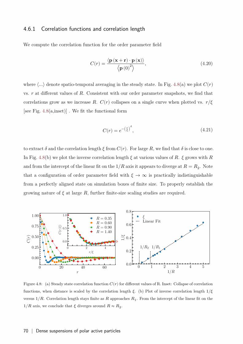
4.6.1 Correlation functions and correlation length
We compute the correlation function for the order parameter field
𝐶(𝑟) = ⟨𝐩 (𝐱 + 𝐫) ⋅ 𝐩 (𝐱)⟩⟨𝐩 (0)2⟩
, (4.20)
where ⟨…⟩ denote spatio-temporal averaging in the steady state. In Fig. 4.8(a) we plot 𝐶(𝑟)vs. 𝑟 at different values of 𝑅. Consistent with our order parameter snapshots, we find that
correlations grow as we increase 𝑅. 𝐶(𝑟) collapses on a single curve when plotted vs. 𝑟/𝜉[see Fig. 4.8(a,inset)] . We fit the functional form
𝐶(𝑟) = 𝑒−( 𝑟𝜉 )𝛿
, (4.21)
to extract 𝛿 and the correlation length 𝜉 from 𝐶(𝑟). For large 𝑅, we find that 𝛿 is close to one.
In Fig. 4.8(b) we plot the inverse correlation length 𝜉 at various values of 𝑅. 𝜉 grows with 𝑅and from the intercept of the linear fit on the 1/𝑅 axis it appears to diverge at 𝑅 = 𝑅2. Note
that a configuration of order parameter field with 𝜉 → ∞ is practically indistinguishable
from a perfectly aligned state on simulation boxes of finite size. To properly establish the
growing nature of 𝜉 at large 𝑅, further finite-size scaling studies are required.
0 20 40 60r
0.00
0.25
0.50
0.75
1.00
C(r
)
0 2 4
r/ξ
0.0
0.5
1.0
C(r/ξ
)
R = 0.35R = 0.60R = 0.90R = 1.40
0 1 2 3 4 51/R
0.0
0.2
0.4
0.6
0.8
1/ξ
1/R11/R2
ξLinear Fit
Figure 4.8: (a) Steady state correlation function 𝐶(𝑟) for different values of R. Inset: Collapse of correlation
functions, when distance is scaled by the correlation length 𝜉. (b) Plot of inverse correlation length 1/𝜉versus 1/𝑅. Correlation length stays finite as 𝑅 approaches 𝑅1. From the intercept of the linear fit on the
1/𝑅 axis, we conclude that 𝜉 diverges around 𝑅 ≈ 𝑅2.
70 | Dense suspensions of polar active particles
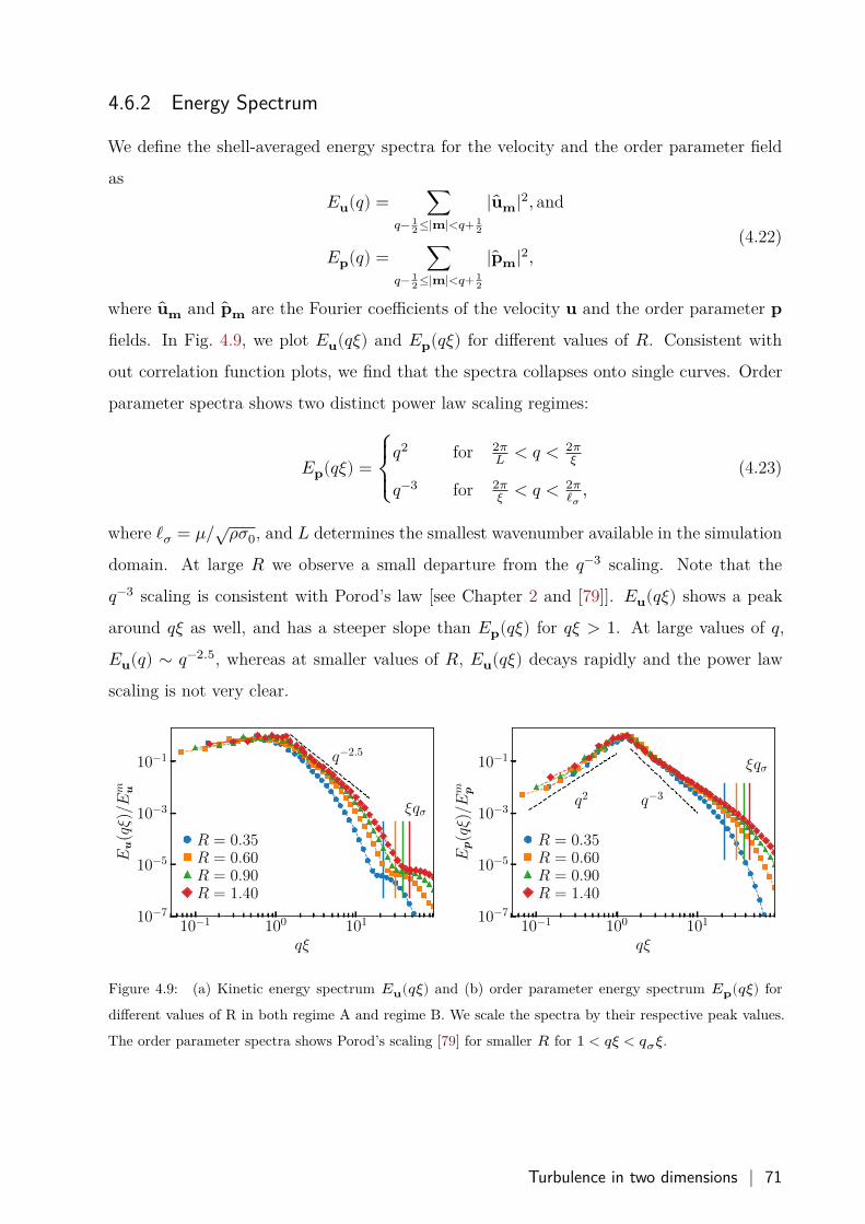
4.6.2 Energy Spectrum
We define the shell-averaged energy spectra for the velocity and the order parameter field
as𝐸𝐮(𝑞) = ∑
𝑞− 12 ≤|𝐦|<𝑞+ 1
2
|��𝐦|2, and
𝐸𝐩(𝑞) = ∑𝑞− 1
2 ≤|𝐦|<𝑞+ 12
|��𝐦|2,(4.22)
where ��𝐦 and ��𝐦 are the Fourier coefficients of the velocity 𝐮 and the order parameter 𝐩fields. In Fig. 4.9, we plot 𝐸𝐮(𝑞𝜉) and 𝐸𝐩(𝑞𝜉) for different values of 𝑅. Consistent with
out correlation function plots, we find that the spectra collapses onto single curves. Order
parameter spectra shows two distinct power law scaling regimes:
𝐸𝐩(𝑞𝜉) =⎧{⎨{⎩
𝑞2 for 2𝜋𝐿 < 𝑞 < 2𝜋
𝜉
𝑞−3 for 2𝜋𝜉 < 𝑞 < 2𝜋
ℓ𝜎,
(4.23)
where ℓ𝜎 = 𝜇/√𝜌𝜎0, and 𝐿 determines the smallest wavenumber available in the simulation
domain. At large 𝑅 we observe a small departure from the 𝑞−3 scaling. Note that the
𝑞−3 scaling is consistent with Porod’s law [see Chapter 2 and [79]]. 𝐸𝐮(𝑞𝜉) shows a peak
around 𝑞𝜉 as well, and has a steeper slope than 𝐸𝐩(𝑞𝜉) for 𝑞𝜉 > 1. At large values of 𝑞,
𝐸𝐮(𝑞) ∼ 𝑞−2.5, whereas at smaller values of 𝑅, 𝐸𝐮(𝑞𝜉) decays rapidly and the power law
scaling is not very clear.
10−1 100 101
qξ
10−7
10−5
10−3
10−1
Eu(qξ)/E
m u
q−2.5
ξqσ
R = 0.35R = 0.60R = 0.90R = 1.40
10−1 100 101
qξ
10−7
10−5
10−3
10−1
Ep(qξ)/E
m p
q−3q2
ξqσ
R = 0.35R = 0.60R = 0.90R = 1.40
Figure 4.9: (a) Kinetic energy spectrum 𝐸𝐮(𝑞𝜉) and (b) order parameter energy spectrum 𝐸𝐩(𝑞𝜉) for
different values of R in both regime A and regime B. We scale the spectra by their respective peak values.
The order parameter spectra shows Porod’s scaling [79] for smaller 𝑅 for 1 < 𝑞𝜉 < 𝑞𝜎𝜉.
Turbulence in two dimensions | 71
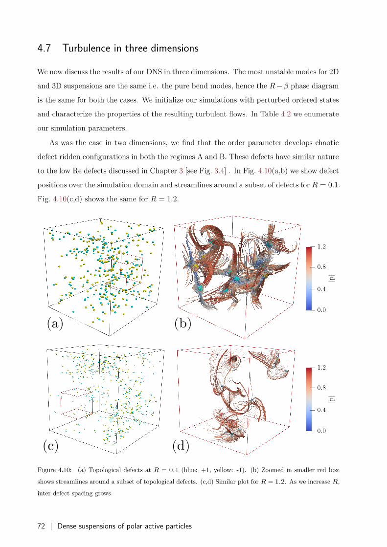
4.7 Turbulence in three dimensions
We now discuss the results of our DNS in three dimensions. The most unstable modes for 2D
and 3D suspensions are the same i.e. the pure bend modes, hence the 𝑅 − 𝛽 phase diagram
is the same for both the cases. We initialize our simulations with perturbed ordered states
and characterize the properties of the resulting turbulent flows. In Table 4.2 we enumerate
our simulation parameters.
As was the case in two dimensions, we find that the order parameter develops chaotic
defect ridden configurations in both the regimes A and B. These defects have similar nature
to the low Re defects discussed in Chapter 3 [see Fig. 3.4] . In Fig. 4.10(a,b) we show defect
positions over the simulation domain and streamlines around a subset of defects for 𝑅 = 0.1.
Fig. 4.10(c,d) shows the same for 𝑅 = 1.2.
Figure 4.10: (a) Topological defects at 𝑅 = 0.1 (blue: +1, yellow: -1). (b) Zoomed in smaller red box
shows streamlines around a subset of topological defects. (c,d) Similar plot for 𝑅 = 1.2. As we increase 𝑅,
inter-defect spacing grows.
72 | Dense suspensions of polar active particles
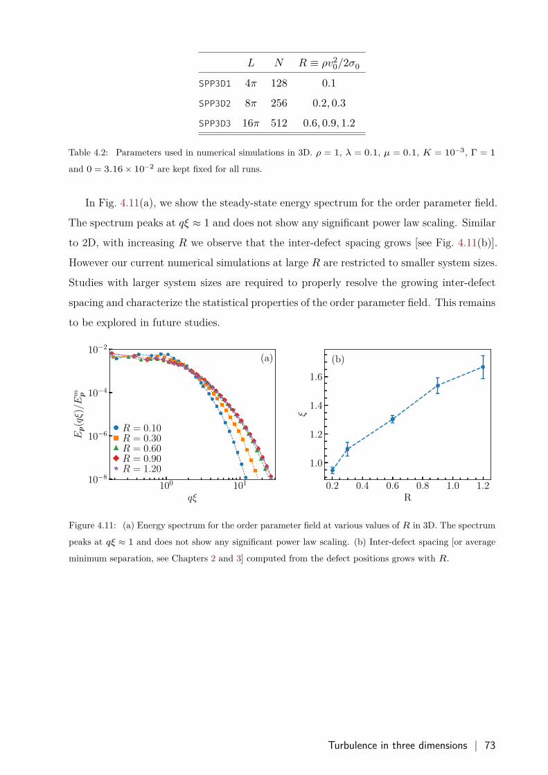
𝐿 𝑁 𝑅 ≡ 𝜌𝑣20/2𝜎0
SPP3D1 4𝜋 128 0.1SPP3D2 8𝜋 256 0.2, 0.3SPP3D3 16𝜋 512 0.6, 0.9, 1.2
Table 4.2: Parameters used in numerical simulations in 3D. 𝜌 = 1, 𝜆 = 0.1, 𝜇 = 0.1, 𝐾 = 10−3, Γ = 1and 0 = 3.16 × 10⁻² are kept fixed for all runs.
In Fig. 4.11(a), we show the steady-state energy spectrum for the order parameter field.
The spectrum peaks at 𝑞𝜉 ≈ 1 and does not show any significant power law scaling. Similar
to 2D, with increasing 𝑅 we observe that the inter-defect spacing grows [see Fig. 4.11(b)].
However our current numerical simulations at large 𝑅 are restricted to smaller system sizes.
Studies with larger system sizes are required to properly resolve the growing inter-defect
spacing and characterize the statistical properties of the order parameter field. This remains
to be explored in future studies.
100 101
qξ
10−8
10−6
10−4
10−2
Ep(qξ)/E
m p
(a)
R = 0.10R = 0.30R = 0.60R = 0.90R = 1.20
0.2 0.4 0.6 0.8 1.0 1.2R
1.0
1.2
1.4
1.6
ξ
(b)
Figure 4.11: (a) Energy spectrum for the order parameter field at various values of 𝑅 in 3D. The spectrum
peaks at 𝑞𝜉 ≈ 1 and does not show any significant power law scaling. (b) Inter-defect spacing [or average
minimum separation, see Chapters 2 and 3] computed from the defect positions grows with 𝑅.
Turbulence in three dimensions | 73
4.8 Comparison with Malthusian suspensions
In an earlier study [55] [see also Section 1.4 and [135]], we have studied the stability of
ordered state in Malthusian suspensions where the birth-death processes occur at time
scales smaller than the time scales of collective motion, and can restore the concentration
to its equilibrium value quickly. Concentration is a fast variable in such systems and is
ignored in the hydrodynamic description. The equations of motion are
𝜌 (𝜕𝑡𝐮 + 𝐮.∇𝐮) = −∇𝑃 + 𝜇∇2𝐮 − ∇.𝚺,
𝜕𝑡𝐩 + (𝐮 + 𝑣0𝐩).∇𝐩 = 𝜆𝐒.𝐩 + 𝛀.𝐩 + Γ𝐡,
∇ ⋅ 𝐮 = 0.
(4.24)
Here all the phenomenological parameters take their values at the equilibrium concentration
maintained by the birth-death processes. Note that the order parameter is not incompress-
ible for Malthusian suspensions. We now highlight the similarities and differences between
dense and Malthusian suspensions.
4.8.1 Linear stability analysis
For a suspension described by (4.1), concentration fluctuations couple only to the two-
dimensional splay-bend modes [55, 135]. Any constraints imposed on the number conser-
vation equation will then also affect only these modes. Thus, the linear stability of the
twist-bend modes and crucially the most unstable pure bend modes is independent of the
dynamics of the concentration fluctuations. The differences between the Malthusian and
dense suspensions arise in the form of allowed topological defects and the nature of steady
states in regimes A and B, which we describe below.
4.8.2 Non equilibrium steady states
For dense suspensions, vortices and saddles are the only allowed topological defects. On the
other hand, asters are the dominant structures for Malthusian suspensions. In Fig. 4.12 we
show various structures observed in the steady-state at different values of 𝑅 for Malthusian
and dense suspensions. Malthusian suspensions show a non-equilibrium flocking transition
from aster-riddled defect turbulent states to aligned but phase turbulent states as R crosses
from regime A to B. We do not observe any such transition for incompressible suspensions,
where we observe vortices even in regime B. The absence of phase-turbulence is corroborated
74 | Dense suspensions of polar active particles
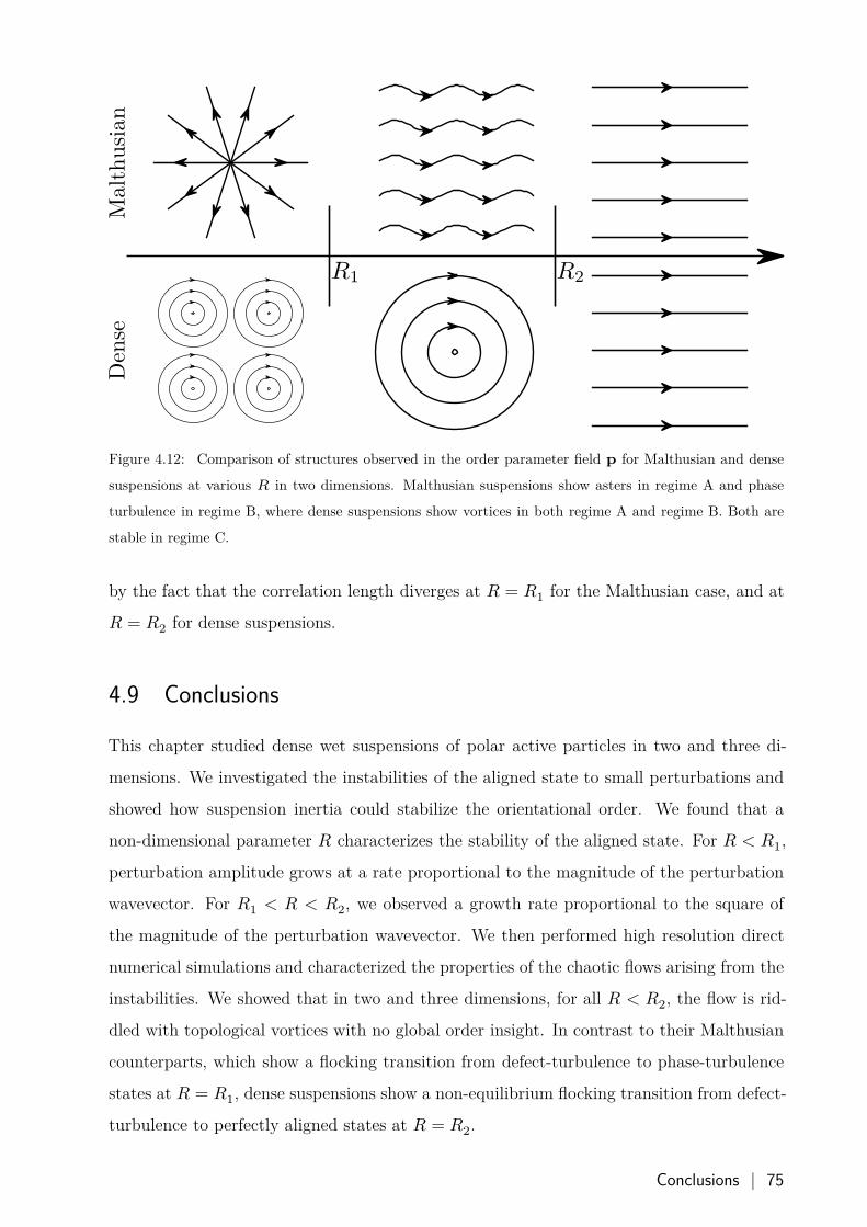
Figure 4.12: Comparison of structures observed in the order parameter field 𝐩 for Malthusian and dense
suspensions at various 𝑅 in two dimensions. Malthusian suspensions show asters in regime A and phase
turbulence in regime B, where dense suspensions show vortices in both regime A and regime B. Both are
stable in regime C.
by the fact that the correlation length diverges at 𝑅 = 𝑅1 for the Malthusian case, and at
𝑅 = 𝑅2 for dense suspensions.
4.9 Conclusions
This chapter studied dense wet suspensions of polar active particles in two and three di-
mensions. We investigated the instabilities of the aligned state to small perturbations and
showed how suspension inertia could stabilize the orientational order. We found that a
non-dimensional parameter 𝑅 characterizes the stability of the aligned state. For 𝑅 < 𝑅1,
perturbation amplitude grows at a rate proportional to the magnitude of the perturbation
wavevector. For 𝑅1 < 𝑅 < 𝑅2, we observed a growth rate proportional to the square of
the magnitude of the perturbation wavevector. We then performed high resolution direct
numerical simulations and characterized the properties of the chaotic flows arising from the
instabilities. We showed that in two and three dimensions, for all 𝑅 < 𝑅2, the flow is rid-
dled with topological vortices with no global order insight. In contrast to their Malthusian
counterparts, which show a flocking transition from defect-turbulence to phase-turbulence
states at 𝑅 = 𝑅1, dense suspensions show a non-equilibrium flocking transition from defect-
turbulence to perfectly aligned states at 𝑅 = 𝑅2.
Conclusions | 75

Chapter 5
Population fluctuations in growing bacteria colonies
In earlier chapters, we have investigated systems where the activity manifests as self-
propelling particles. In this chapter, we focus on a colony of nonmotile bacteria growing
on a hard agar surface. Here, the activity arises not from the particle motility, but the
birth-death processes. At the colony front, bacteria repeatedly grow and divide at the expense
of nutrients and push each other in the process. These steric repulsions between the bacteria
result in an expanding colony. Population fluctuations intrinsic to any birth-death process
become essential for such systems, especially at the growing front where the number of
organisms is small compared to the colony’s interior. We investigate how these fluctuations
and nutrient availability can affect the growing colony’s morphology. We find that the
population fluctuations and nutrient-dependent bacteria diffusion are sufficient to cause the
morphological transition from finger-like branched fronts to smooth fronts upon increasing
nutrient concentration.
5.1 Introduction
Pattern formation is one of the fascinating feature observed in a broad range of natural
phenomena [18, 138, 139]. For example, colonies of bacteria growing on a Petri dish exhibit
a large variety of intricate spatial patterns ranging from compact circular growth, concentric
rings to long branched patterns [11, 13, 140–145]. The colony morphology depends on
various factors such as nutrient concentration, cell motility, birth-death dynamics, and
other chemical and physical variables [146–154].
In Fig. 5.1, we show various morphological patterns observed in Escherichia Coli colonies
growing on a hard agar surface in different environment settings. The colonies show compact
| 77
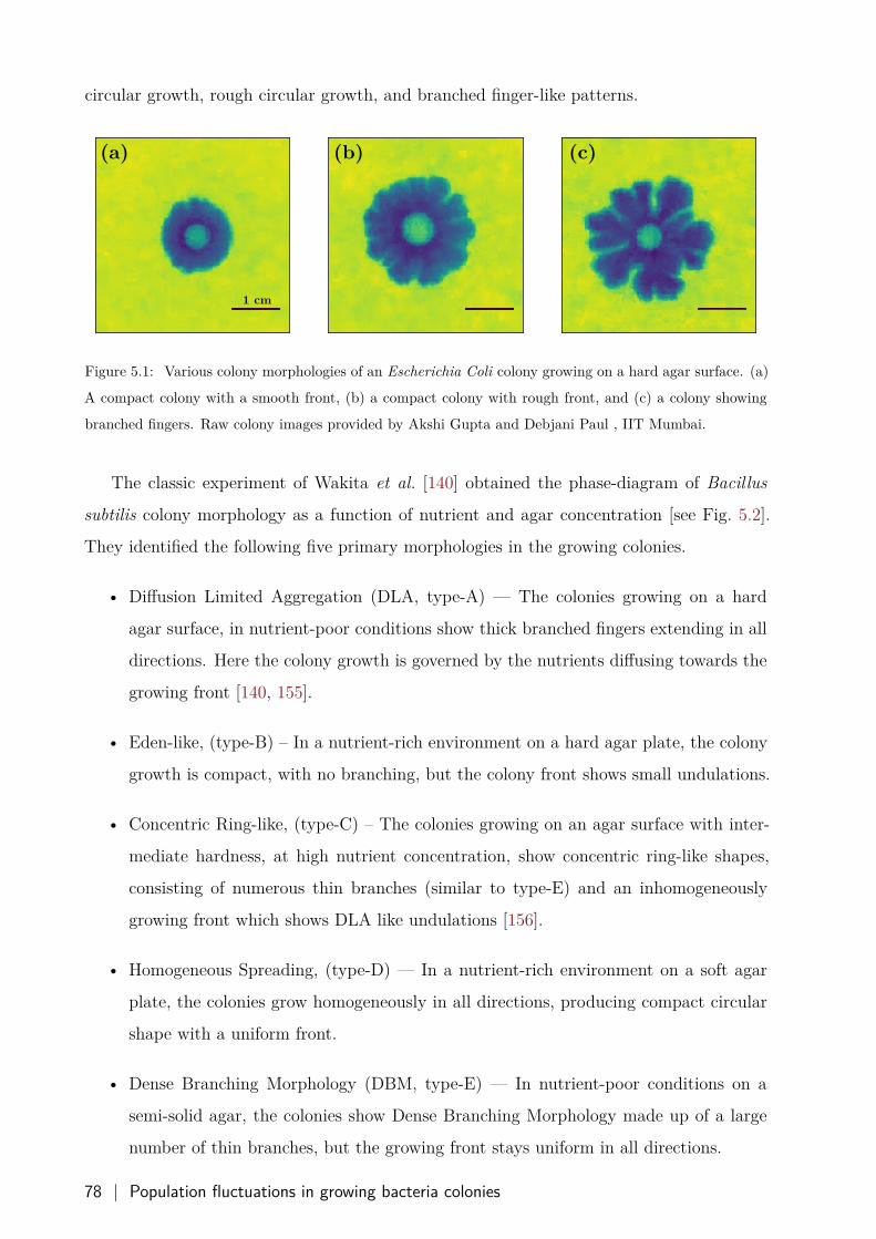
circular growth, rough circular growth, and branched finger-like patterns.
(a) (b) (c)
1 cm
Figure 5.1: Various colony morphologies of an Escherichia Coli colony growing on a hard agar surface. (a)
A compact colony with a smooth front, (b) a compact colony with rough front, and (c) a colony showing
branched fingers. Raw colony images provided by Akshi Gupta and Debjani Paul , IIT Mumbai.
The classic experiment of Wakita et al. [140] obtained the phase-diagram of Bacillus
subtilis colony morphology as a function of nutrient and agar concentration [see Fig. 5.2].
They identified the following five primary morphologies in the growing colonies.
• Diffusion Limited Aggregation (DLA, type-A) — The colonies growing on a hard
agar surface, in nutrient-poor conditions show thick branched fingers extending in all
directions. Here the colony growth is governed by the nutrients diffusing towards the
growing front [140, 155].
• Eden-like, (type-B) – In a nutrient-rich environment on a hard agar plate, the colony
growth is compact, with no branching, but the colony front shows small undulations.
• Concentric Ring-like, (type-C) – The colonies growing on an agar surface with inter-
mediate hardness, at high nutrient concentration, show concentric ring-like shapes,
consisting of numerous thin branches (similar to type-E) and an inhomogeneously
growing front which shows DLA like undulations [156].
• Homogeneous Spreading, (type-D) — In a nutrient-rich environment on a soft agar
plate, the colonies grow homogeneously in all directions, producing compact circular
shape with a uniform front.
• Dense Branching Morphology (DBM, type-E) — In nutrient-poor conditions on a
semi-solid agar, the colonies show Dense Branching Morphology made up of a large
number of thin branches, but the growing front stays uniform in all directions.
78 | Population fluctuations in growing bacteria colonies
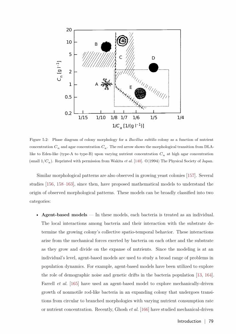
Figure 5.2: Phase diagram of colony morphology for a Bacillus subtilis colony as a function of nutrient
concentration 𝐶𝑛 and agar concentration 𝐶𝑎. The red arrow shows the morphological transition from DLA-
like to Eden-like (type-A to type-B) upon varying nutrient concentration 𝐶𝑛 at high agar concentration
(small 1/𝐶𝑎). Reprinted with permission from Wakita et al. [140]. ©(1994) The Physical Society of Japan.
Similar morphological patterns are also observed in growing yeast colonies [157]. Several
studies [156, 158–163], since then, have proposed mathematical models to understand the
origin of observed morphological patterns. These models can be broadly classified into two
categories:
• Agent-based models — In these models, each bacteria is treated as an individual.
The local interactions among bacteria and their interaction with the substrate de-
termine the growing colony’s collective spatio-temporal behavior. These interactions
arise from the mechanical forces exerted by bacteria on each other and the substrate
as they grow and divide on the expanse of nutrients. Since the modeling is at an
individual’s level, agent-based models are used to study a broad range of problems in
population dynamics. For example, agent-based models have been utilized to explore
the role of demographic noise and genetic drifts in the bacteria population [13, 164].
Farrell et al. [165] have used an agent-based model to explore mechanically-driven
growth of nonmotile rod-like bacteria in an expanding colony that undergoes transi-
tions from circular to branched morphologies with varying nutrient consumption rate
or nutrient concentration. Recently, Ghosh et al. [166] have studied mechanical-driven
Introduction | 79
spontaneous phase-segregation of nonmotile, rod-shaped bacteria in the presence of
self-secreted extracellular polymeric substances in a growing biofilm.
• Reaction-Diffusion models — In such models, we treat bacteria density and nutri-
ent concentration as fields described by a set of continuum equations. Diffusive terms
model the bacteria and nutrient motility, and the birth-death processes are modeled
with a reaction term. Perhaps the most widely used reaction-diffusion equation is the
Fisher-Kolmogorov-Piscunoff-Petrovsky equation (FKPP) [56, 57]
𝜕𝑡𝜌 = 𝐷∇2𝜌 + 𝛾𝜌 (1 − 𝜌) , (5.1)
where 𝜌 is the bacteria density fraction, 𝛾 is the growth rate, and 𝐷 is the bacteria
diffusivity. (5.1) has been successfully used to model homogeneous spreading of bac-
teria on a soft-agar plate and in a nutrient-rich environment. Several studies have
incorporated the effect of the nutrient concentration and bacteria motility by coupling
(5.1) with an additional equation for each of these variables to obtain different mor-
phological patterns discussed above [11, 13, 140–145]. Studies designed to investigate
the role of demographic noise use the stochastic variants of (5.1) [13, 57, 167–170].
In this chapter, we explore how the morphology of a colony of nonmotile bacteria growing
on a hard agar substrate changes with varying initial nutrient concentration. Our study is
designed to mimic the experiments of Wakita et al. [140], which show a transition from DLA-
like morphology (type-A) to Eden-like patterns (type-B) when initial nutrient concentration
is increased at a fixed (high) agar concentration (shown by the red arrow in Fig. 5.2).
Earlier studies [11, 143, 163, 171, 172] attribute observed morphological patterns to
substrate properties such as irregularities of the agar substrate [171], substrate hardness
that depends on the agar concentration [11], and local lubrication created by the bacteria
[163]. These models ignore the population fluctuations which are intrinsic to birth-death
processes, and describe the colony growth in a mean-field setting. Recent studies [13, 173,
174] have however shown that fluctuations play an important role in determining the growth,
competition, and cooperation in growing bacterial colonies. Population fluctuations become
essential at the growing front, where the number of bacteria is very small compared to the
colony interior, and cannot be ignored. In particular, Kessler and Levine [173] show that
the stochastic noise leads to diffusive instabilities in the otherwise homogeneously growing
front.
80 | Population fluctuations in growing bacteria colonies
We present here a stochastic continuum model, to study the role of initial nutrient
concentration on the spreading of nonmotile bacteria colony on a hard agar surface. Our
model takes into account the population fluctuation and we assume that the substrate is uni-
form, lacks any inhomogeneities, and ignore substrate-bacteria interaction. Our numerical
experiments show that population fluctuations and nutrient-dependent bacteria diffusivity
destabilize the front and lead to the formation of finger-like patterns in nutrient-deprived
conditions. We find that increasing initial nutrient concentration leads to faster growing
colonies, and the front speed agrees with the mean-field predictions. The front structure
undergoes a transition from a branching pattern to an Eden pattern on increasing the initial
nutrient condition.
In the rest of the chapter, we discuss our continuum model, numerical methods and
results in details.
5.2 Construction of the stochastic continuum model
In this section we outline the construction of the continuum model for a reaction-diffusion
bacteria-nutrient system [56, 57, 160, 175]. We model the growth and division of the bacteria
on the expense of the nutrients using the following reaction
𝐵 + 𝐹 → 𝐵 + 𝐵 at a rate 𝑘, (5.2)
where 𝐵 denotes bacteria and 𝐹 denotes nutrient. A bacterium eats a unit nutrient at a
rate 𝑘 per unit time and divides into two. Ignoring the spatial variations and defining 𝜌𝐵(𝑡)and 𝑐(𝑡) as the bacteria and nutrient number density at time 𝑡, the bacteria density fraction
𝜌(𝑡) = 𝜌𝐵/(𝜌𝐵 + 𝑐) obeys the equation
𝑑𝜌𝑑𝑡 = 𝛾𝜌 (1 − 𝜌) + 𝜇√𝜌 (1 − 𝜌)𝜂 (𝑡) . (5.3)
Here 𝛾 = 𝑘 (𝜌𝐵 + 𝑐) is the growth rate, 𝜇 controls the noise strength and 𝜂(𝑡) is a Gaussian
white noise with ⟨𝜂(𝑡)⟩ = 0, ⟨𝜂 (𝑡) 𝜂 (𝑡′)⟩ = 𝛿 (𝑡 − 𝑡′), and the angular brackets indicate
averaging over noise realizations.
In a spatially extended system where the bacteria are allowed to diffuse and the nutri-
ent concentration is uniform everywhere, (5.3) leads to the stochastic Fisher-Kolmogorov-
Piscunoff-Petrovsky (sFKPP) equation
𝜕𝑡𝜌 = 𝐷∇2𝜌 + 𝛾𝜌 (1 − 𝜌) + 𝜇√𝜌 (1 − 𝜌)𝜂(𝐱, 𝑡) (5.4)
Construction of the stochastic continuum model | 81
where 𝐷 is the diffusivity and 𝜂(𝐱, 𝑡) is Gaussian white noise with ⟨𝜂(𝐱, 𝑡)⟩ = 0, ⟨𝜂(𝐱, 𝑡)𝜂 (𝐱′, 𝑡′)⟩ =𝜹 (𝐱 − 𝐱′) 𝛿 (𝑡 − 𝑡′).
In the absence of population fluctuations (𝜇 = 0), (5.4) reduces to the mean-field FKPP
equation (5.1), which admits wave solutions of the form 𝜌(𝐱, 𝑡) = 𝑤 (𝐱 − 𝑉 𝑡). The front
propagation velocity 𝑉 satisfies the criterion 𝑉 ≥ 2√𝐷𝛾, and for sufficiently sharp initial
fronts the minimum speed 𝑉 = 2√𝐷𝛾 is selected [56, 57, 167]. For the sFKPP equation
(5.4), the stochastic term leads to corrections in the selected speed [167, 176, 177]. In the
weak noise limit, where the dimensionless noise strength 𝜇/ (𝐷𝛾)1/4 < 1, the selected front
velocity for the sFKPP equation is 𝑉 ≈ √𝐷𝛾 [2 − 𝜋2/(4 log2 𝜇)], whereas in the strong
noise limit where 𝜇/ (𝐷𝛾)1/4 > 1 the front velocity is 𝑉 = 2𝐷𝛾/𝜇2 [167].
5.2.1 Nutrient-Bacteria (NB) models
We now write our nutrient-bacteria (NB) models in which, similar to (5.2), bacteria con-
sumes nutrient and divides at a rate 𝛾 per unit biomass while diffusing through space. In
the mean-field setting, the bacteria-nutrient dynamics can be described by the diffusive
Fisher-Kolmogorov equations [56, 57, 160]:
𝜕𝑡𝑐 = 𝐷∇2𝑐 − 𝛾𝜌𝐵𝑐,
𝜕𝑡𝜌𝐵 = 𝐷𝐵∇2𝜌𝐵 + 𝛾𝜌𝐵𝑐.(5.5)
Here, 𝜌𝐵(𝐱, 𝑡) is the bacterial number density and 𝑐 (𝐱, 𝑡) is the nutrient concentration at
position 𝐱 and time 𝑡, 𝐷𝐵 and 𝐷 are diffusion coefficient of bacteria and nutrient, and total
number density over the entire domain 𝐿−2 ∫ [𝜌𝐵(𝐱, 𝑡) + 𝑐(𝐱, 𝑡)] 𝑑𝑥𝑑𝑦 remains conserved.
Variants of the NB model (5.5) but with more complicated reaction and diffusion terms
have been used earlier to investigate the transition from type-A to type-B [56, 160, 163].
However, these mean-field models ignore the role of population fluctuations in the system.
We incorporate population fluctuations in the NB model by adding to it a multiplicative
noise term similar to the sFKPP equation (5.4) [167, 170, 178]. The stochastic NB (sNB)
model that we use, written in terms of the total density 𝜌𝑇 (𝐱, 𝑡) ≡ 𝜌𝐵(𝐱, 𝑡) + 𝑐(𝐱, 𝑡) and
the bacterial number density 𝜌𝐵(𝐱, 𝑡) is
𝜕𝑡𝜌𝑇 = 𝐷𝐵∇2𝜌𝐵 + 𝐷∇2𝑐,
𝜕𝑡𝜌𝐵 = 𝐷𝐵∇2𝜌𝐵 + 𝛾𝜌𝐵 (𝜌𝑇 − 𝜌𝐵) + 𝜇√𝜌𝐵(𝜌𝑇 − 𝜌𝐵)𝜂(𝐱, 𝑡).(5.6)
The first equation simply tells us that the total number density can only vary due to the
diffusion of nutrient and bacteria (5.2) conserves the total number of particles. The second
equation describes the growth of the colony on the expanse of limited available nutrients.
82 | Population fluctuations in growing bacteria colonies
In the sNB model, even in the absence of nutrients, the bacteria will diffuse through
space. However, in a more realistic case the motility of the colony might depend upon
nutrient concentration as well, wherein scarce nutrient conditions will lead to very less
or no movement at all. The diffusion of passive nutrients remains unchanged. Following
Golding et al. [160], we incorporate this effect by using a non-linear nutrient dependent
bacteria diffusivity to get the sNBNL model
𝜕𝑡𝜌𝑇 = 𝐷𝐵∇ ⋅ (𝑐∇𝜌𝐵) + 𝐷∇2𝑐, and
𝜕𝑡𝜌𝐵 = 𝐷𝐵∇ ⋅ (𝑐∇𝜌𝐵) + 𝛾𝜌𝐵 (𝜌𝑇 − 𝜌𝐵) + 𝜇√𝜌𝐵 (𝜌𝑇 − 𝜌𝐵)𝜂(𝐱, 𝑡).(5.7)
In what follows, we present a systematic study of how bacterial front speed and mor-
phology is modified because of nutrient concentration, population fluctuations, bacterial
diffusivity, and nutrient diffusivity using direct numerical simulations (DNS) of sNB and
sNBNL models.
5.3 Numerical methods
We perform simulations of sNB and sNBNL models on a square domain of length 𝐿 dis-
cretized with 𝑁2 collocation points. We use a second-order centered finite-difference scheme
to numerically evaluate the spatial derivatives and impose Neumann boundary conditions
on all sides of the simulation domain. For time marching, we use a variant of the operator
splitting scheme proposed in Refs [175, 179] as described below. We initialize the bacteria
and nutrient number density as
𝜌𝐵 (𝐱, 0) = 12 [1 − tanh {𝑎 (𝑦 − 𝑏)}] ,
𝑐 (𝐱, 0) = 𝐶0 {1 − 𝜌𝐵(𝐱, 0)} .(5.8)
The constants 𝑎 and 𝑏 fix the width and the position of the colony front, and 𝐶0 fixes
the initial nutrient concentration.
Constants in the simulations: In the macroscopic experiments of colony growth, the
number of bacteria is significant. To mimic the same, we fix the strength of population
noise to a small value 𝜇 = 5 × 10⁻² in all our simulations. Our simulations are then in the
weak noise limit, where 𝜇/ (𝐷𝐵𝛾)1/4 < 1. We also fix 𝐷 = 10−1 to mimic the slow diffusion
of nutrients on a hard agar plate and choose our timescale such that 𝛾 = 1.
Numerical methods | 83
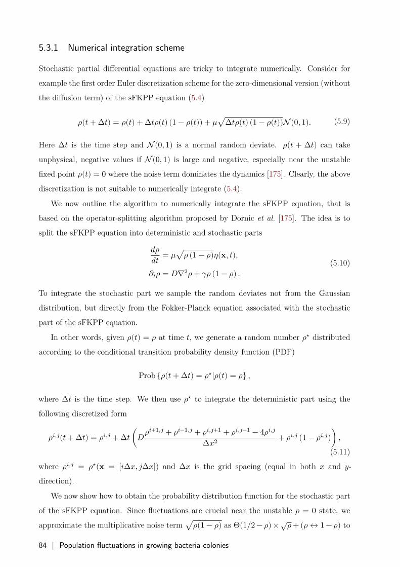
5.3.1 Numerical integration scheme
Stochastic partial differential equations are tricky to integrate numerically. Consider for
example the first order Euler discretization scheme for the zero-dimensional version (without
the diffusion term) of the sFKPP equation (5.4)
𝜌(𝑡 + Δ𝑡) = 𝜌(𝑡) + Δ𝑡𝜌(𝑡) (1 − 𝜌(𝑡)) + 𝜇√Δ𝑡𝜌(𝑡) (1 − 𝜌(𝑡))N (0, 1). (5.9)
Here Δ𝑡 is the time step and N (0, 1) is a normal random deviate. 𝜌(𝑡 + Δ𝑡) can take
unphysical, negative values if N (0, 1) is large and negative, especially near the unstable
fixed point 𝜌(𝑡) = 0 where the noise term dominates the dynamics [175]. Clearly, the above
discretization is not suitable to numerically integrate (5.4).
We now outline the algorithm to numerically integrate the sFKPP equation, that is
based on the operator-splitting algorithm proposed by Dornic et al. [175]. The idea is to
split the sFKPP equation into deterministic and stochastic parts
𝑑𝜌𝑑𝑡 = 𝜇√𝜌 (1 − 𝜌)𝜂(𝐱, 𝑡),
𝜕𝑡𝜌 = 𝐷∇2𝜌 + 𝛾𝜌 (1 − 𝜌) .(5.10)
To integrate the stochastic part we sample the random deviates not from the Gaussian
distribution, but directly from the Fokker-Planck equation associated with the stochastic
part of the sFKPP equation.
In other words, given 𝜌(𝑡) = 𝜌 at time 𝑡, we generate a random number 𝜌⋆ distributed
according to the conditional transition probability density function (PDF)
Prob {𝜌(𝑡 + Δ𝑡) = 𝜌⋆|𝜌(𝑡) = 𝜌} ,
where Δ𝑡 is the time step. We then use 𝜌⋆ to integrate the deterministic part using the
following discretized form
𝜌𝑖,𝑗(𝑡 + Δ𝑡) = 𝜌𝑖,𝑗 + Δ𝑡 (𝐷𝜌𝑖+1,𝑗 + 𝜌𝑖−1,𝑗 + 𝜌𝑖,𝑗+1 + 𝜌𝑖,𝑗−1 − 4𝜌𝑖,𝑗
Δ𝑥2 + 𝜌𝑖,𝑗 (1 − 𝜌𝑖,𝑗)) ,(5.11)
where 𝜌𝑖,𝑗 = 𝜌⋆(𝐱 = [𝑖Δ𝑥, 𝑗Δ𝑥]) and Δ𝑥 is the grid spacing (equal in both 𝑥 and 𝑦-
direction).
We now show how to obtain the probability distribution function for the stochastic part
of the sFKPP equation. Since fluctuations are crucial near the unstable 𝜌 = 0 state, we
approximate the multiplicative noise term √𝜌(1 − 𝜌) as Θ(1/2 − 𝜌) × √𝜌 + (𝜌 ↔ 1 − 𝜌) to
84 | Population fluctuations in growing bacteria colonies
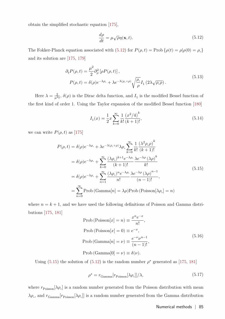
obtain the simplified stochastic equation [175],
𝑑𝜌𝑑𝑡 = 𝜇√𝜌𝜂(𝐱, 𝑡). (5.12)
The Fokker-Planck equation associated with (5.12) for 𝑃(𝜌, 𝑡) = Prob {𝜌(𝑡) = 𝜌|𝜌(0) = 𝜌∘}and its solution are [175, 179]
𝜕𝑡𝑃 (𝜌, 𝑡) = 𝜇2
2 𝜕2𝜌 [𝜌𝑃 (𝜌, 𝑡)] ,
𝑃 (𝜌, 𝑡) = 𝛿(𝜌)𝑒−𝜆𝜌∘ + 𝜆𝑒−𝜆(𝜌∘+𝜌)√𝜌∘𝜌 𝐼1 (2𝜆√𝜌∘𝜌) .
(5.13)
Here 𝜆 = 2𝜇2𝑡 , 𝛿(𝜌) is the Dirac delta function, and 𝐼1 is the modified Bessel function of
the first kind of order 1. Using the Taylor expansion of the modified Bessel function [180]
𝐼1(𝑥) = 12𝑥
∞∑𝑘=0
1𝑘!
(𝑥2/4)𝑘
(𝑘 + 1)! , (5.14)
we can write 𝑃(𝜌, 𝑡) as [175]
𝑃(𝜌, 𝑡) = 𝛿(𝜌)𝑒−𝜆𝜌∘ + 𝜆𝑒−𝜆(𝜌∘+𝜌)𝜆𝜌∘∞
∑𝑘=0
1𝑘!
(𝜆2𝜌∘𝜌)𝑘
(𝑘 + 1)!
= 𝛿(𝜌)𝑒−𝜆𝜌∘ +∞
∑𝑘=0
(𝜆𝜌∘)𝑘+1𝑒−𝜆𝜌∘
(𝑘 + 1)!𝜆𝑒−𝜆𝜌 (𝜆𝜌)𝑘
𝑘!
= 𝛿(𝜌)𝑒−𝜆𝜌∘ +∞
∑𝑛=1
(𝜆𝜌∘)𝑛𝑒−𝜆𝜌∘
𝑛!𝜆𝑒−𝜆𝜌 (𝜆𝜌)𝑛−1
(𝑛 − 1)! ,
=∞
∑𝑛=0
Prob (Gamma[𝑛] = 𝜆𝜌)Prob (Poisson[𝜆𝜌∘] = 𝑛)
(5.15)
where 𝑛 = 𝑘 + 1, and we have used the following definitions of Poisson and Gamma distri-
butions [175, 181]Prob (Poisson[𝑥] = 𝑛) ≡ 𝑥𝑛𝑒−𝑥
𝑛! ,
Prob (Poisson[𝑥] = 0) ≡ 𝑒−𝑥,
Prob (Gamma[𝑛] = 𝜈) ≡ 𝑒−𝜈𝜈𝑛−1
(𝑛 − 1)! ,
Prob (Gamma[0] = 𝜈) ≡ 𝛿(𝜈).
(5.16)
Using (5.15) the solution of (5.12) is the random number 𝜌⋆ generated as [175, 181]
𝜌⋆ = 𝑟Gamma[𝑟Poisson[𝜆𝜌∘]]/𝜆, (5.17)
where 𝑟Poisson[𝜆𝜌∘] is a random number generated from the Poisson distribution with mean
𝜆𝜌∘, and 𝑟Gamma[𝑟Poisson[𝜆𝜌∘]] is a random number generated from the Gamma distribution
Numerical methods | 85
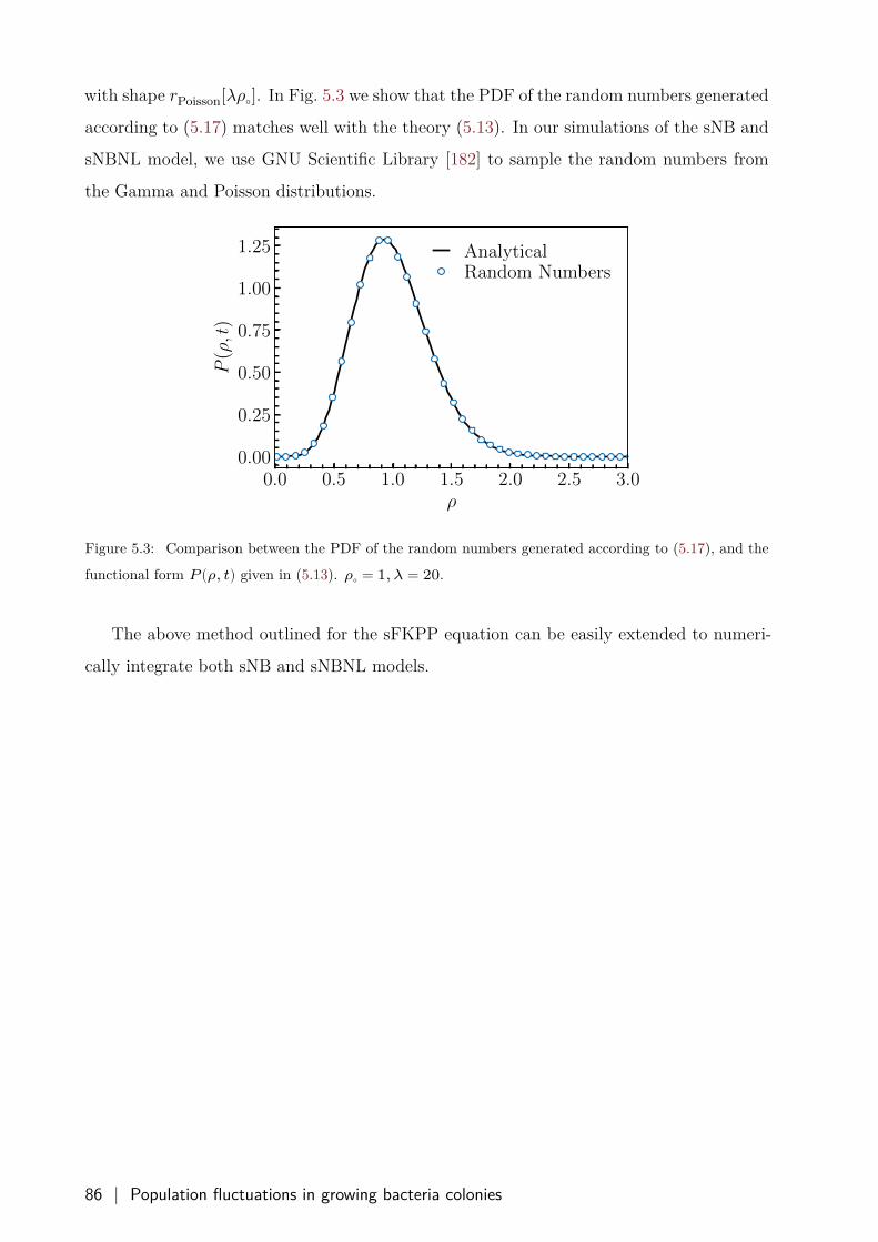
with shape 𝑟Poisson[𝜆𝜌∘]. In Fig. 5.3 we show that the PDF of the random numbers generated
according to (5.17) matches well with the theory (5.13). In our simulations of the sNB and
sNBNL model, we use GNU Scientific Library [182] to sample the random numbers from
the Gamma and Poisson distributions.
0.0 0.5 1.0 1.5 2.0 2.5 3.0ρ
0.00
0.25
0.50
0.75
1.00
1.25
P(ρ,t
)
AnalyticalRandom Numbers
Figure 5.3: Comparison between the PDF of the random numbers generated according to (5.17), and the
functional form 𝑃(𝜌, 𝑡) given in (5.13). 𝜌∘ = 1, 𝜆 = 20.
The above method outlined for the sFKPP equation can be easily extended to numeri-
cally integrate both sNB and sNBNL models.
86 | Population fluctuations in growing bacteria colonies
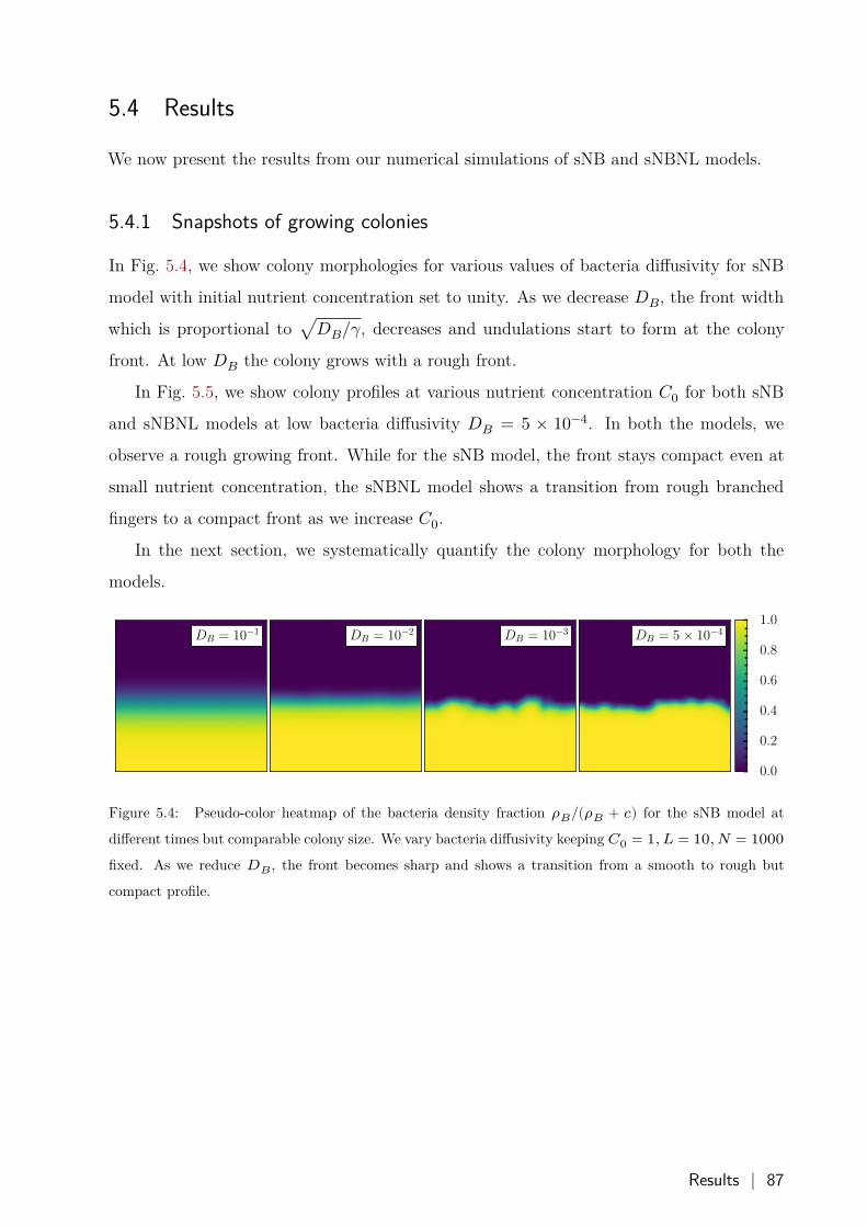
5.4 Results
We now present the results from our numerical simulations of sNB and sNBNL models.
5.4.1 Snapshots of growing colonies
In Fig. 5.4, we show colony morphologies for various values of bacteria diffusivity for sNB
model with initial nutrient concentration set to unity. As we decrease 𝐷𝐵, the front width
which is proportional to √𝐷𝐵/𝛾, decreases and undulations start to form at the colony
front. At low 𝐷𝐵 the colony grows with a rough front.
In Fig. 5.5, we show colony profiles at various nutrient concentration 𝐶0 for both sNB
and sNBNL models at low bacteria diffusivity 𝐷𝐵 = 5 × 10⁻⁴. In both the models, we
observe a rough growing front. While for the sNB model, the front stays compact even at
small nutrient concentration, the sNBNL model shows a transition from rough branched
fingers to a compact front as we increase 𝐶0.
In the next section, we systematically quantify the colony morphology for both the
models.
DB = 10−1 DB = 10−2 DB = 10−3 DB = 5× 10⁻⁴
0.0
0.2
0.4
0.6
0.8
1.0
Figure 5.4: Pseudo-color heatmap of the bacteria density fraction 𝜌𝐵/(𝜌𝐵 + 𝑐) for the sNB model at
different times but comparable colony size. We vary bacteria diffusivity keeping 𝐶0 = 1, 𝐿 = 10, 𝑁 = 1000fixed. As we reduce 𝐷𝐵, the front becomes sharp and shows a transition from a smooth to rough but
compact profile.
Results | 87
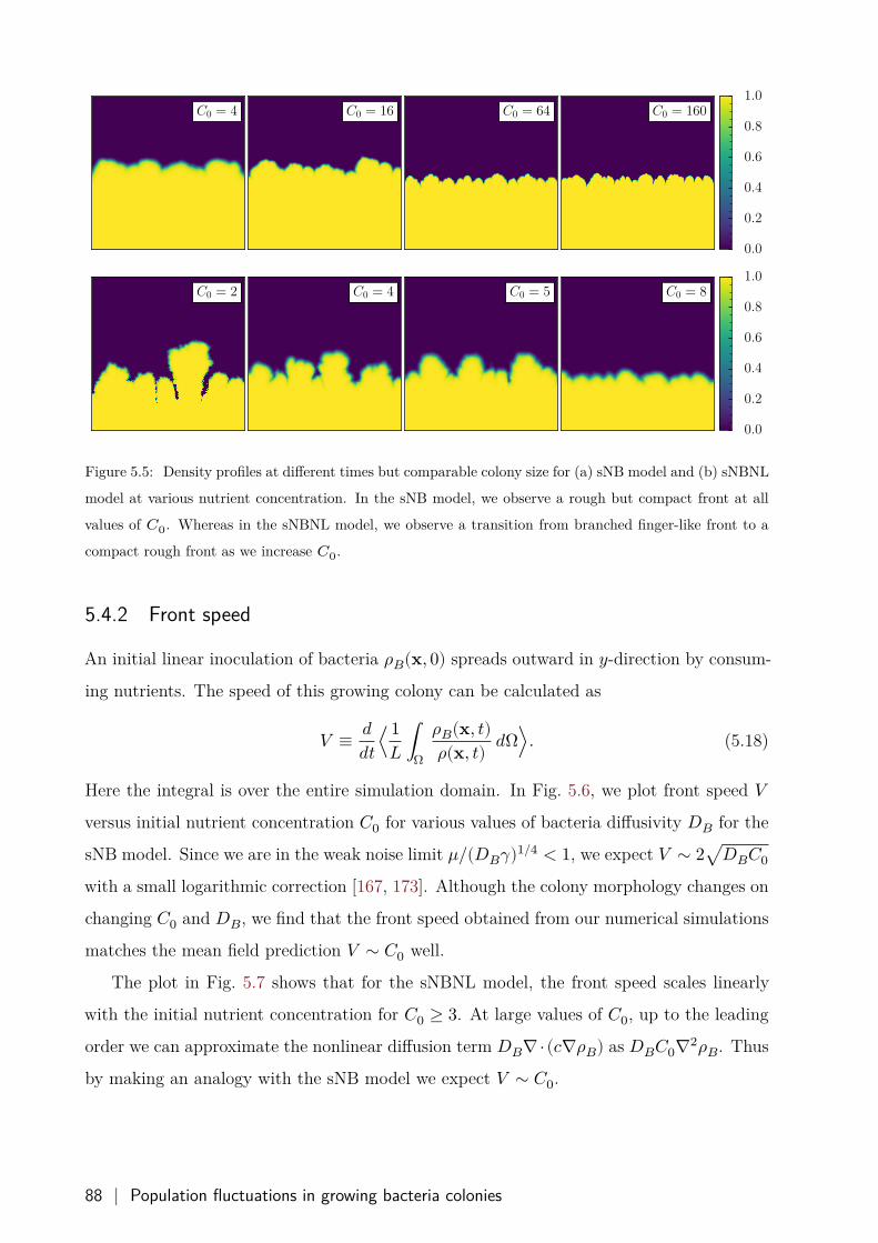
Figure 5.5: Density profiles at different times but comparable colony size for (a) sNB model and (b) sNBNL
model at various nutrient concentration. In the sNB model, we observe a rough but compact front at all
values of 𝐶0. Whereas in the sNBNL model, we observe a transition from branched finger-like front to a
compact rough front as we increase 𝐶0.
5.4.2 Front speed
An initial linear inoculation of bacteria 𝜌𝐵(𝐱, 0) spreads outward in 𝑦-direction by consum-
ing nutrients. The speed of this growing colony can be calculated as
𝑉 ≡ 𝑑𝑑𝑡⟨ 1
𝐿 ∫Ω
𝜌𝐵(𝐱, 𝑡)𝜌(𝐱, 𝑡) 𝑑Ω⟩. (5.18)
Here the integral is over the entire simulation domain. In Fig. 5.6, we plot front speed 𝑉versus initial nutrient concentration 𝐶0 for various values of bacteria diffusivity 𝐷𝐵 for the
sNB model. Since we are in the weak noise limit 𝜇/(𝐷𝐵𝛾)1/4 < 1, we expect 𝑉 ∼ 2√𝐷𝐵𝐶0
with a small logarithmic correction [167, 173]. Although the colony morphology changes on
changing 𝐶0 and 𝐷𝐵, we find that the front speed obtained from our numerical simulations
matches the mean field prediction 𝑉 ∼ 𝐶0 well.
The plot in Fig. 5.7 shows that for the sNBNL model, the front speed scales linearly
with the initial nutrient concentration for 𝐶0 ≥ 3. At large values of 𝐶0, up to the leading
order we can approximate the nonlinear diffusion term 𝐷𝐵∇⋅(𝑐∇𝜌𝐵) as 𝐷𝐵𝐶0∇2𝜌𝐵. Thus
by making an analogy with the sNB model we expect 𝑉 ∼ 𝐶0.
88 | Population fluctuations in growing bacteria colonies
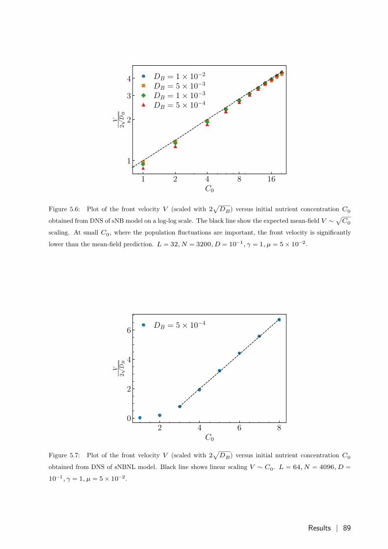
Figure 5.6: Plot of the front velocity 𝑉 (scaled with 2√𝐷𝐵) versus initial nutrient concentration 𝐶0
obtained from DNS of sNB model on a log-log scale. The black line show the expected mean-field 𝑉 ∼ √𝐶0
scaling. At small 𝐶0, where the population fluctuations are important, the front velocity is significantly
lower than the mean-field prediction. 𝐿 = 32, 𝑁 = 3200, 𝐷 = 10−1, 𝛾 = 1, 𝜇 = 5 × 10⁻².
Figure 5.7: Plot of the front velocity 𝑉 (scaled with 2√𝐷𝐵) versus initial nutrient concentration 𝐶0
obtained from DNS of sNBNL model. Black line shows linear scaling 𝑉 ∼ 𝐶0. 𝐿 = 64, 𝑁 = 4096, 𝐷 =10−1, 𝛾 = 1, 𝜇 = 5 × 10⁻².
Results | 89
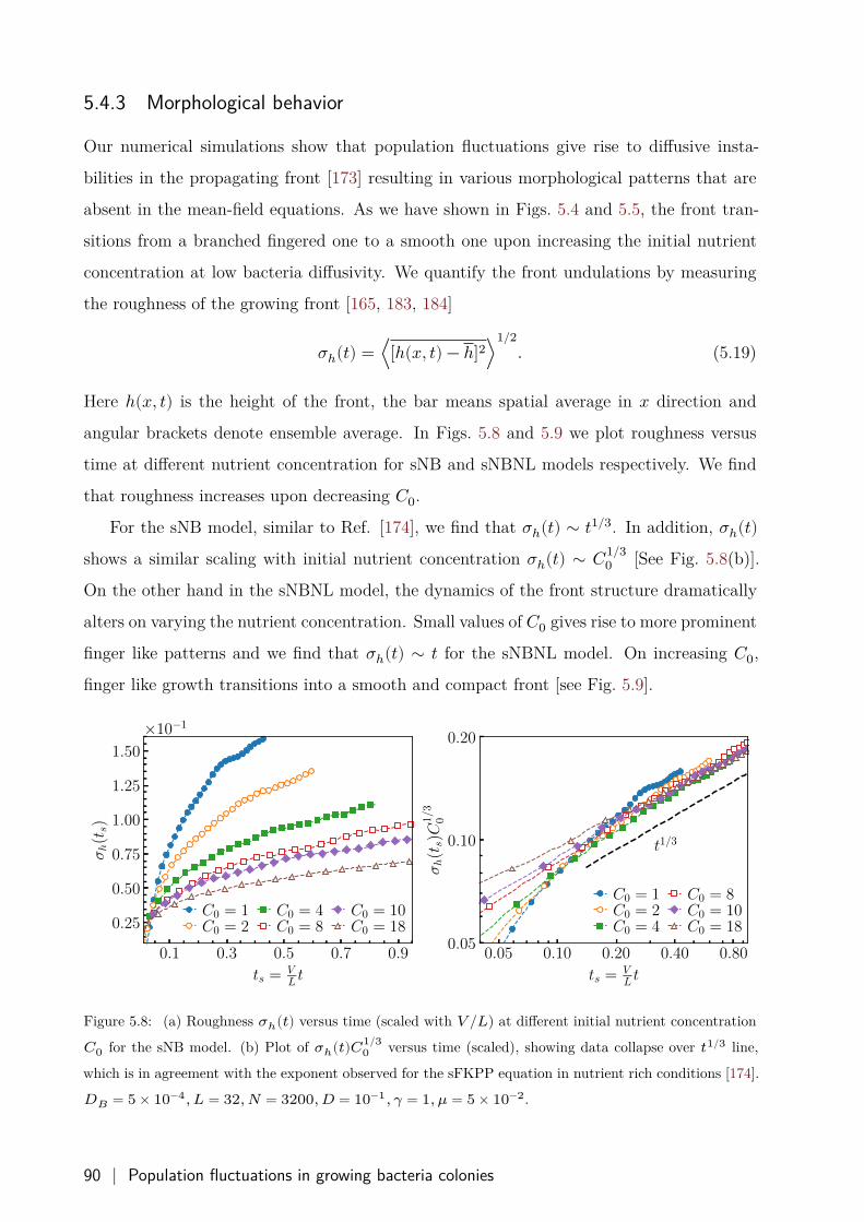
5.4.3 Morphological behavior
Our numerical simulations show that population fluctuations give rise to diffusive insta-
bilities in the propagating front [173] resulting in various morphological patterns that are
absent in the mean-field equations. As we have shown in Figs. 5.4 and 5.5, the front tran-
sitions from a branched fingered one to a smooth one upon increasing the initial nutrient
concentration at low bacteria diffusivity. We quantify the front undulations by measuring
the roughness of the growing front [165, 183, 184]
𝜎ℎ(𝑡) = ⟨[ℎ(𝑥, 𝑡) − ℎ]2⟩1/2
. (5.19)
Here ℎ(𝑥, 𝑡) is the height of the front, the bar means spatial average in 𝑥 direction and
angular brackets denote ensemble average. In Figs. 5.8 and 5.9 we plot roughness versus
time at different nutrient concentration for sNB and sNBNL models respectively. We find
that roughness increases upon decreasing 𝐶0.
For the sNB model, similar to Ref. [174], we find that 𝜎ℎ(𝑡) ∼ 𝑡1/3. In addition, 𝜎ℎ(𝑡)shows a similar scaling with initial nutrient concentration 𝜎ℎ(𝑡) ∼ 𝐶1/3
0 [See Fig. 5.8(b)].
On the other hand in the sNBNL model, the dynamics of the front structure dramatically
alters on varying the nutrient concentration. Small values of 𝐶0 gives rise to more prominent
finger like patterns and we find that 𝜎ℎ(𝑡) ∼ 𝑡 for the sNBNL model. On increasing 𝐶0,
finger like growth transitions into a smooth and compact front [see Fig. 5.9].
0.1 0.3 0.5 0.7 0.9
ts = VL t
0.25
0.50
0.75
1.00
1.25
1.50
σh(ts)
×10−1
C0 = 1C0 = 2
C0 = 4C0 = 8
C0 = 10C0 = 18
0.05 0.10 0.20 0.40 0.80
ts = VL t
0.05
0.10
0.20
σh(ts)C
1/3
0
t1/3
C0 = 1C0 = 2C0 = 4
C0 = 8C0 = 10C0 = 18
Figure 5.8: (a) Roughness 𝜎ℎ(𝑡) versus time (scaled with 𝑉 /𝐿) at different initial nutrient concentration
𝐶0 for the sNB model. (b) Plot of 𝜎ℎ(𝑡)𝐶1/30 versus time (scaled), showing data collapse over 𝑡1/3 line,
which is in agreement with the exponent observed for the sFKPP equation in nutrient rich conditions [174].
𝐷𝐵 = 5 × 10⁻⁴, 𝐿 = 32, 𝑁 = 3200, 𝐷 = 10−1, 𝛾 = 1, 𝜇 = 5 × 10⁻².
90 | Population fluctuations in growing bacteria colonies
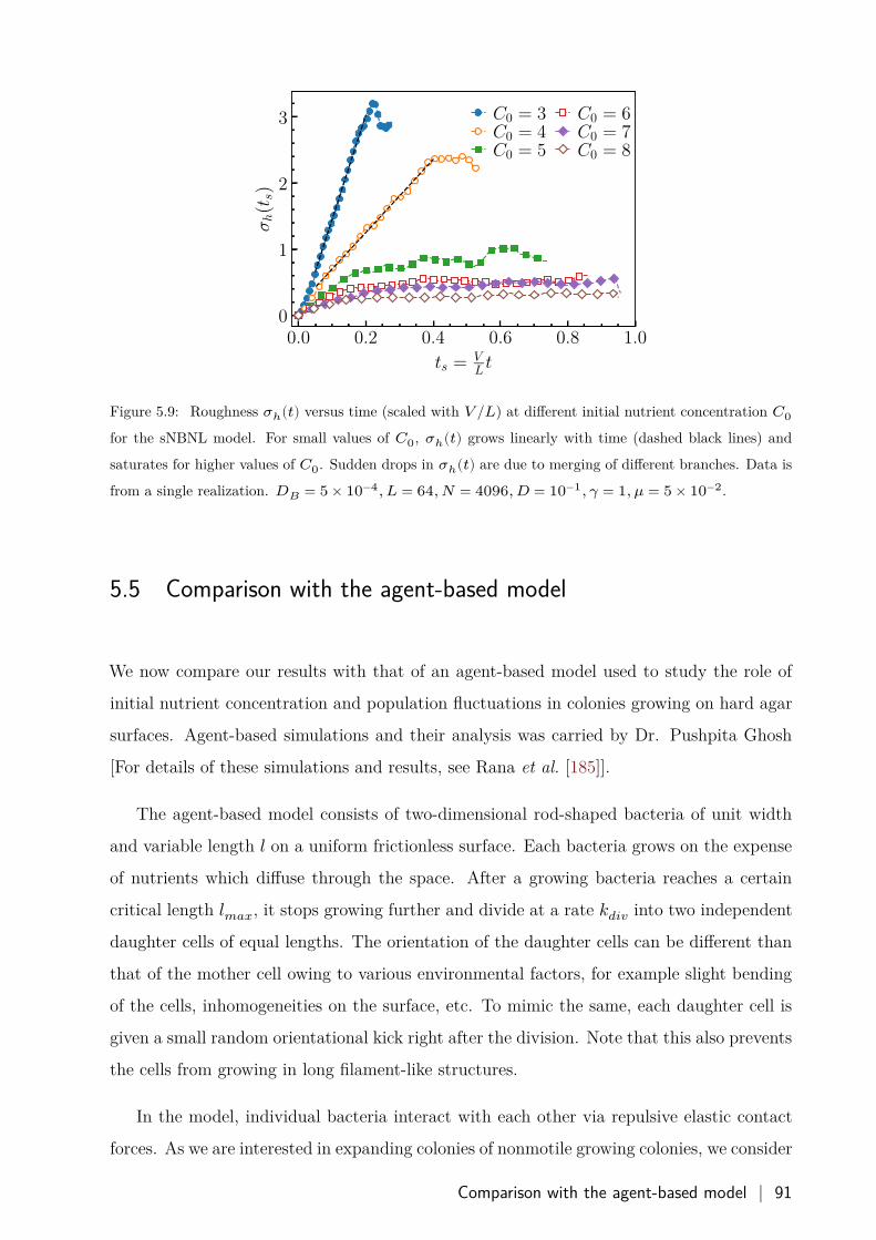
0.0 0.2 0.4 0.6 0.8 1.0
ts = VL t
0
1
2
3
σh(ts)
C0 = 3C0 = 4C0 = 5
C0 = 6C0 = 7C0 = 8
Figure 5.9: Roughness 𝜎ℎ(𝑡) versus time (scaled with 𝑉 /𝐿) at different initial nutrient concentration 𝐶0
for the sNBNL model. For small values of 𝐶0, 𝜎ℎ(𝑡) grows linearly with time (dashed black lines) and
saturates for higher values of 𝐶0. Sudden drops in 𝜎ℎ(𝑡) are due to merging of different branches. Data is
from a single realization. 𝐷𝐵 = 5 × 10⁻⁴, 𝐿 = 64, 𝑁 = 4096, 𝐷 = 10−1, 𝛾 = 1, 𝜇 = 5 × 10⁻².
5.5 Comparison with the agent-based model
We now compare our results with that of an agent-based model used to study the role of
initial nutrient concentration and population fluctuations in colonies growing on hard agar
surfaces. Agent-based simulations and their analysis was carried by Dr. Pushpita Ghosh
[For details of these simulations and results, see Rana et al. [185]].
The agent-based model consists of two-dimensional rod-shaped bacteria of unit width
and variable length 𝑙 on a uniform frictionless surface. Each bacteria grows on the expense
of nutrients which diffuse through the space. After a growing bacteria reaches a certain
critical length 𝑙𝑚𝑎𝑥, it stops growing further and divide at a rate 𝑘𝑑𝑖𝑣 into two independent
daughter cells of equal lengths. The orientation of the daughter cells can be different than
that of the mother cell owing to various environmental factors, for example slight bending
of the cells, inhomogeneities on the surface, etc. To mimic the same, each daughter cell is
given a small random orientational kick right after the division. Note that this also prevents
the cells from growing in long filament-like structures.
In the model, individual bacteria interact with each other via repulsive elastic contact
forces. As we are interested in expanding colonies of nonmotile growing colonies, we consider
Comparison with the agent-based model | 91
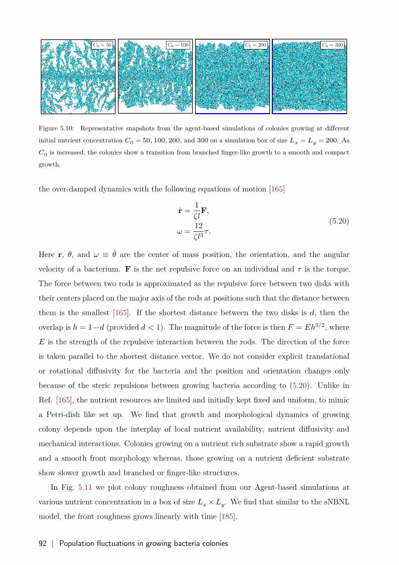
Figure 5.10: Representative snapshots from the agent-based simulations of colonies growing at different
initial nutrient concentration 𝐶0 = 50, 100, 200, and 300 on a simulation box of size 𝐿𝑥 = 𝐿𝑦 = 200. As
𝐶0 is increased, the colonies show a transition from branched finger-like growth to a smooth and compact
growth.
the over-damped dynamics with the following equations of motion [165]
𝐫 = 1𝜁𝑙𝐅,
𝜔 = 12𝜁𝑙3 𝜏.
(5.20)
Here 𝐫, 𝜃, and 𝜔 ≡ 𝜃 are the center of mass position, the orientation, and the angular
velocity of a bacterium. 𝐅 is the net repulsive force on an individual and 𝜏 is the torque.
The force between two rods is approximated as the repulsive force between two disks with
their centers placed on the major axis of the rods at positions such that the distance between
them is the smallest [165]. If the shortest distance between the two disks is 𝑑, then the
overlap is ℎ = 1−𝑑 (provided 𝑑 < 1). The magnitude of the force is then 𝐹 = 𝐸ℎ3/2, where
𝐸 is the strength of the repulsive interaction between the rods. The direction of the force
is taken parallel to the shortest distance vector. We do not consider explicit translational
or rotational diffusivity for the bacteria and the position and orientation changes only
because of the steric repulsions between growing bacteria according to (5.20). Unlike in
Ref. [165], the nutrient resources are limited and initially kept fixed and uniform, to mimic
a Petri-dish like set up. We find that growth and morphological dynamics of growing
colony depends upon the interplay of local nutrient availability, nutrient diffusivity and
mechanical interactions. Colonies growing on a nutrient rich substrate show a rapid growth
and a smooth front morphology whereas, those growing on a nutrient deficient substrate
show slower growth and branched or finger-like structures.
In Fig. 5.11 we plot colony roughness obtained from our Agent-based simulations at
various nutrient concentration in a box of size 𝐿𝑥 × 𝐿𝑦. We find that similar to the sNBNL
model, the front roughness grows linearly with time [185].
92 | Population fluctuations in growing bacteria colonies
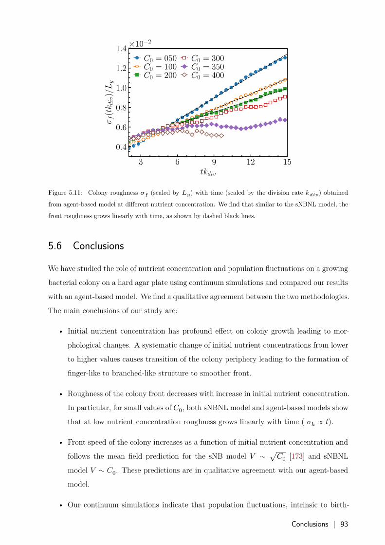
3 6 9 12 15tkdiv
0.4
0.6
0.8
1.0
1.2
1.4
σf(tkdiv
)/Ly
×10−2
C0 = 050C0 = 100C0 = 200
C0 = 300C0 = 350C0 = 400
Figure 5.11: Colony roughness 𝜎𝑓 (scaled by 𝐿𝑦) with time (scaled by the division rate 𝑘𝑑𝑖𝑣) obtained
from agent-based model at different nutrient concentration. We find that similar to the sNBNL model, the
front roughness grows linearly with time, as shown by dashed black lines.
5.6 Conclusions
We have studied the role of nutrient concentration and population fluctuations on a growing
bacterial colony on a hard agar plate using continuum simulations and compared our results
with an agent-based model. We find a qualitative agreement between the two methodologies.
The main conclusions of our study are:
• Initial nutrient concentration has profound effect on colony growth leading to mor-
phological changes. A systematic change of initial nutrient concentrations from lower
to higher values causes transition of the colony periphery leading to the formation of
finger-like to branched-like structure to smoother front.
• Roughness of the colony front decreases with increase in initial nutrient concentration.
In particular, for small values of 𝐶0, both sNBNL model and agent-based models show
that at low nutrient concentration roughness grows linearly with time ( 𝜎ℎ ∝ 𝑡).
• Front speed of the colony increases as a function of initial nutrient concentration and
follows the mean field prediction for the sNB model 𝑉 ∼ √𝐶0 [173] and sNBNL
model 𝑉 ∼ 𝐶0. These predictions are in qualitative agreement with our agent-based
model.
• Our continuum simulations indicate that population fluctuations, intrinsic to birth-
Conclusions | 93
death processes can explain the transition from branched finger-like growth to smoothly
growing colonies on increasing initial nutrient concentration.
Although our present model only considers bacterial growth in a mono layer on surface,
there is a definite scope to extend our model in three-dimensions to study the growth
dynamics of bacteria forming biofilm-like structures. Bacteria growth and development
in three-dimensions might lead to complex morphologies as an outcome of interactions of
bacteria with surface and extracellular matrix [186]. Moreover, it would also be interesting
to investigate the spatio temporal dynamics of coexisting species using the ideas we present
here.
94 | Population fluctuations in growing bacteria colonies
Chapter 6
Turbulence on DGX architecture: a GPGPU pseu-dospectral solver
In this chapter, we present a general purpose GPU based (GPGPU) pseudospectral solver
for the Navier-Stokes equation. First, we describe the pseudospectral algorithm and its
GPGPU implementation. We then discuss the performance of the pseudospectral algorithm
on the DGX architecture. We will show how the DGX architecture with its powerful GPU
cards and high bandwidth NVLINK communication switches is an ideal platform to perform
discrete numerical simulations of the Navier-Stokes equation at moderate resolutions of size
5123 − 20483.
6.1 Introduction
Finally, there is a physical problem that is common to many fields, that is very
old, and that has not been solved. It is not the problem of finding new fundamental
particles, but something left over from a long time ago –over a hundred years.
Nobody in physics has really been able to analyze it mathematically satisfactorily
in spite of its importance to the sister sciences. It is the analysis of circulating or
turbulent fluids.
– Richard Feynman
Turbulence is often touted as the last unsolved problem of classical physics. Several re-
searchers have tried to understand it both via experimental and analytical means. Perhaps,
the most significant breakthrough was achieved by Kolmogorov in his seminal work in the
early 1940s [187, 188]. Kolmogorov’s theory of turbulence assumes the fluid flow to be sta-
| 95
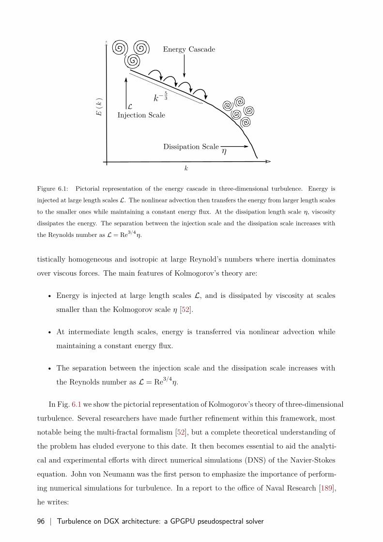
Energy Cascade
Dissipation Scale
Injection Scale
Figure 6.1: Pictorial representation of the energy cascade in three-dimensional turbulence. Energy is
injected at large length scales L. The nonlinear advection then transfers the energy from larger length scales
to the smaller ones while maintaining a constant energy flux. At the dissipation length scale 𝜂, viscosity
dissipates the energy. The separation between the injection scale and the dissipation scale increases with
the Reynolds number as L = Re3/4𝜂.
tistically homogeneous and isotropic at large Reynold’s numbers where inertia dominates
over viscous forces. The main features of Kolmogorov’s theory are:
• Energy is injected at large length scales L, and is dissipated by viscosity at scales
smaller than the Kolmogorov scale 𝜂 [52].
• At intermediate length scales, energy is transferred via nonlinear advection while
maintaining a constant energy flux.
• The separation between the injection scale and the dissipation scale increases with
the Reynolds number as L = Re3/4𝜂.
In Fig. 6.1 we show the pictorial representation of Kolmogorov’s theory of three-dimensional
turbulence. Several researchers have made further refinement within this framework, most
notable being the multi-fractal formalism [52], but a complete theoretical understanding of
the problem has eluded everyone to this date. It then becomes essential to aid the analyti-
cal and experimental efforts with direct numerical simulations (DNS) of the Navier-Stokes
equation. John von Neumann was the first person to emphasize the importance of perform-
ing numerical simulations for turbulence. In a report to the office of Naval Research [189],
he writes:
96 | Turbulence on DGX architecture: a GPGPU pseudospectral solver
...our intuitive relationship to the subject is still too loose—not having succeeded
at anything like deep mathematical penetration in any part of the subject, we are
still quite disoriented as to the relevant factors, and as to the proper analytical
machinery to be used.
Under these conditions there might be some hope to “break the deadlock” by extensive, but
well-planned, computational efforts. It must be admitted that the problems in question are
too vast to be solved by a direct computational attack, that is, by an outright calculation of a
representative family of special cases. There are, however, strong indications that one could
name certain strategic points in this complex, where relevant information must be obtainable
by direct calculations. If this is properly done, and the operation is then repeated on the
basis of broader information then becoming available, etc., there is a reasonable chance of
effecting real penetrations into this complex of problems and gradually developing a useful,
intuitive relationship to it. This should, in the end, make an attack with analytical methods,
that is truly more mathematical, possible.
– John von Neumann
He further remarks on the spatial resolution required and the capabilities of machines
of that era,
... even a linear resolution of 1:8 would require following 83 = 512 spatial
points and a linear resolution of 1:20 would already call for 203 = 8000 points.
The machines which one can hope to use in the immediate future will hardly be
able to exceed the first limit and none that is in sight for several years to come is
likely to get much beyond the second one. ...
– John von Neumann
As Neumann pointed out, it was hopeless to even perform a simulation with a resolution
of 83 grid points at that time, and it remained so until the computation capacity of the
machines improved dramatically. Simulations with large enough resolution required to
understand the dynamics of the turbulent flows became possible only after Patterson and
Orszag introduced the pseudospectral methods in the late 1960s and early 1970s [190–194].
Leveraging the newly introduced Cooley-Turkey algorithm for the Fourier transforms [195],
they performed the first pseudospectral simulations with a spatial resolution of 323 on a
cubic domain of side 2𝜋 and achieved a Taylor-microscale Reynolds number Re𝜆 ∼ 20 [190].
Since then, the computational capacity of the machines has increased by order of mag-
nitudes, and we have come far ahead of the 83 simulations Neumann proposed in the 1950s.
Introduction | 97
The advent of parallel computing using the MPI-framework has allowed the researchers to
conduct high-resolution DNSs of the Navier-Stokes equation, which have played a crucial
role in improving our understanding of turbulent flows. In this regard, the 40963 DNS of
fluid turbulence by Kaneda et al. [125] is a landmark. Further attempts have been made to
increase the grid-resolution and to the best of our knowledge, Iyer et al. [196] have achieved
the highest resolution of 163843 using the pseudospectral algorithm.
While the distributed memory clusters with thousands of CPU cores, communicating
via MPI-framework, dominated the high-performance computing (HPC) in the 1990s and
2000s, recent advances in HPC have come in terms of general-purpose GPU (GPGPU)
computing. Over the past decade, several algorithms like Molecular dynamics, Lattice-
Boltzmann methods have been successfully ported over to GPU based architecture with
impressive performance gains. Researchers have also tried to port FFT algorithms onto
distributed-GPU machines but with poor results. Unlike Lattice-Boltzmann, Molecular
Dynamics or Finite-difference based methods for solving partial differential equations, where
only the neighbor CPUs or GPUs communicate with each other, computing FFTs requires
all-to-all communication, which is the primary reason behind poor performance observed
for distributed-GPU FFT algorithms.
The issue is further aggravated by the fact that on traditional distributed-GPU ma-
chines, GPU-GPU communication takes place via CPUs. To communicate with a remote
GPU, first, the GPU transfers data to its host CPU via PCIe channels, which then commu-
nicates with the host CPU of the remote GPU via MPI interconnect, and finally, the remote
CPU transfers the data to the remote GPU. As a result of these significant communication
bottlenecks, roughly 80% of the total execution time for the FFTs on distributed GPU ma-
chines is spent in the communication phase alone, and the maximum achieved performance
is < 1% of the peak performance [197–199].
Recently introduced DGX architecture attempts to alleviate these issues. On a DGX
machine, the GPUs communicate directly via high bandwidth NVLINK switches, thus
eliminating the need to communicate with the CPUs. Further, each GPU card has a
significantly larger computational capacity and device memory than the earlier available
cards. In this chapter, we show how with enhancements on both the computational and
communication sides, DGX architecture presents as an ideal platform to perform moderate
resolution DNS of the Navier-Stokes equation.
The rest of the chapter is organized as follows. We begin by outlining the theory behind
98 | Turbulence on DGX architecture: a GPGPU pseudospectral solver
the pseudospectral algorithm. Then we present a brief overview of the DGX architecture and
discuss the performance of FFT algorithms. We then describe the GPGPU implementation
of the pseudospectral algorithm and show how it performs on the DGX architecture. We
conclude the chapter by highlighting significant advantages and limitations of the DGX
architecture and a roadmap of our future work.
6.2 Pseudospectral algorithm for the Navier-Stokes equation
The dynamics of Newtonian flows is described by the Navier-Stokes equation [52, 200, 201]
𝜕𝑡𝐮 = −∇𝑃 + 𝐮 × 𝝎 + 𝜈∇2𝐮 + 𝐟, (6.1)
where 𝐮(𝐱, 𝑡) is the velocity field, 𝝎(𝐱, 𝑡) = ∇ × 𝐮 is the vorticity field, 𝜈 is the viscosity,
the pressure term 𝑃(𝐱, 𝑡) enforces incompressibility criterion ∇ ⋅ 𝐮 = 0, and 𝐟 is a suitable
driving term which injects energy in the system.
Our goal is to numerically integrate (6.1) on a periodic cubic domain of side 𝐿 discretized
over 𝑁3 collocation points. We use a pseudospectral algorithm [190, 192, 202] where a vector
field 𝐮(𝐱, 𝑡) is represented as a discrete Fourier series expansion 1
𝐮(𝐱, 𝑡) = 1𝑁 ∑
𝐤��𝐤𝑒𝑖𝐤⋅𝐱, (6.2)
where 𝑥𝛼 ∈ 𝐿𝑁 {0, 1, 2 … , 𝑁 − 1}, 𝑘𝛼 ∈ 2𝜋
𝐿 {−𝑁2 + 1, −𝑁
2 + 2, … , 𝑁2 }, and the Fourier am-
plitudes ��𝐤 are defined as ��𝐤 = F𝐤 {𝐮} ≡ ∑𝐱 𝐮(𝐱, 𝑡)𝑒−𝑖𝐤⋅𝐱. In Fourier space (6.1) is
written as𝜕𝑡��𝐤 = −𝑖𝐤𝑃𝐤 + 𝑊𝐤 − 𝜈𝑘2��𝐤 + 𝐟𝐤,
𝐤 ⋅ ��𝐤 = 0,(6.3)
where 𝑊𝐤 = F𝐤 {𝐮 × 𝝎}, 𝑃𝐤 = F𝐤 {𝑃}, 𝐟𝐤 = F𝐤 {𝐟}, and 𝑘2 = 𝐤 ⋅ 𝐤. Taking dot product
of (6.3) with 𝐤 and using the incompressibility constraint 𝐤 ⋅ ��𝐤 = 0 we get
𝑃𝐤 = 𝑖𝐤 ⋅ (𝑊𝐤 + 𝐟𝐤) /𝑘2. (6.4)
Substituting 𝑃𝐤 back in (6.3) we obtain for 𝐤 ≠ 0
𝜕𝑡��𝐤 = −𝜈𝑘2��𝐤 + P ⋅ (𝑊𝐤 + 𝐟𝐤) , (6.5)
where P = I − ���� is the projection operator, and �� = 𝐤/𝑘. For 𝐤 = 0 (6.3) simplifies to
𝜕𝑡��0 = 𝑊0 + 𝐟0. (6.6)1Or a scalar field 𝜙(𝐱, 𝑡) as 𝜙(𝐱, 𝑡) = 1
𝑁 ∑𝐤 𝜙𝐤𝑒𝑖𝐤⋅𝐱.
Pseudospectral algorithm for the Navier-Stokes equation | 99
6.2.1 Integration scheme
We use a second order exponential scheme (ETD2) [112] which relies on exact integration
of the linear terms present in (6.5). Below we outline the derivation of ETD2 scheme. We
begin by rewriting (6.5) as
𝜕𝑡��𝐤 = 𝑐��𝐤 + 𝐹𝐤(𝑡), (6.7)
where 𝑐 = −𝜈𝑘2 and 𝐹𝐤(𝑡) = P ⋅ (𝑊𝐤 + 𝐟𝐤). Multiplying (6.7) with the integrating factor
𝑒−𝑐𝑡 and integrating from 𝑡 to 𝑡 + Δ𝑡 yields
��𝐤(𝑡 + Δ𝑡) = ��𝐤(𝑡)𝑒𝑐Δ𝑡 + 𝑒𝑐Δ𝑡 ∫Δ𝑡
0𝑒−𝑐𝑡′𝐹𝐤(𝑡 + 𝑡′)𝑑𝑡′. (6.8)
For the second order scheme (ETD2), we use the following approximation for 𝐹𝐤(𝑡 + 𝑡′),
𝐹𝐤 (𝑡 + 𝑡′) = 𝐹𝐤(𝑡) + 𝑡′
Δ𝑡 (𝐹𝐤(𝑡) − 𝐹𝐤(𝑡 − Δ𝑡)) + O (Δ𝑡2) ∀ 𝑡′ ∈ [0, Δ𝑡]. (6.9)
Solving the integral in (6.8) with the above approximation gives us the ETD2 scheme for
the Navier-Stokes equation,
��𝐤(𝑡 + Δ𝑡) = ��𝐤(𝑡)𝑒𝑐Δ𝑡 + (1 + 𝑐Δ𝑡)𝑒𝑐Δ𝑡 − 1 − 2𝑐Δ𝑡Δ𝑡𝑐2 𝐹𝐤(𝑡) + 1 + 𝑐Δ𝑡 − 𝑒𝑐Δ𝑡
Δ𝑡𝑐2 𝐹𝐤(𝑡 − Δ𝑡),(6.10)
with a local truncation error 5Δ𝑡3 𝐹𝐤(𝑡)/12. Note that (6.10) requires the knowledge of
both 𝐹𝐤(𝑡) and 𝐹𝐤(𝑡 − Δ𝑡) at all times. Since 𝐹𝐤(𝑡 − Δ𝑡) is not known at 𝑡 = 0, we use a
first order scheme (ETD1)
��𝐤(𝑡 + Δ𝑡) = ��𝐤(𝑡)𝑒𝑐Δ𝑡 + 𝑒𝑐Δ𝑡 − 1𝑐 𝐹𝐤(𝑡), (6.11)
to perform the first integration step that is derived from the approximation that 𝐹𝐤(𝑡) stays
constant in the interval 𝑡 and 𝑡 + Δ𝑡,
𝐹𝐤 (𝑡 + 𝑡′) = 𝐹𝐤(𝑡) + O (Δ𝑡) ∀ 𝑡′ ∈ [0, Δ𝑡]. (6.12)
6.2.2 Computing the nonlinear term
Using the Fourier amplitudes of the velocity 𝐮(𝐱) = ∑𝐩 ��𝐩𝑒𝑖𝐩⋅𝐱 and the vorticity field
𝝎(𝐱) = ∑𝐪 𝝎𝐪𝑒𝑖𝐪⋅𝐱, we can write the nonlinear term 𝐮 × 𝝎 as
(𝐮 × 𝝎)𝛼 = 𝜖𝛼𝛽𝛾𝑢𝛽𝜔𝛾
= 𝜖𝛼𝛽𝛾 ∑𝐩,𝐪
��𝐩,𝛽��𝐪,𝛾𝑒𝑖(𝐩+𝐪)⋅𝐱. (6.13)
100 | Turbulence on DGX architecture: a GPGPU pseudospectral solver
Fourier transform of the above equation gives
𝑊𝐤,𝛼 = F {(𝐮 × 𝝎)𝛼} = 𝜖𝛼𝛽𝛾 ∑𝐩+𝐪=𝐤
��𝐩,𝛽��𝐪,𝛾, (6.14)
where 𝛿 (𝐩 + 𝐪 − 𝐤) is the Kronecker-Delta function.
From (6.14) it is evident that the nonlinear advection term is a convolution in the
Fourier space and computing it will require O (𝑁6) operations. In contrast, computing the
nonlinear term in the real space will only need O (𝑁3) operations. Thus the nonlinear term
can be computed in the real space, and then transformed to the Fourier space to perform
numerical integration provided efficient methods for the Fourier transforms exist. Orszag
and Patterson [193] realized that expensive convolutions could be avoided by leveraging
Fast Fourier Transform (FFT) algorithms which require O (𝑁3 log 𝑁3) operations. In the so
called Pseudospectral method, at each time step the velocity and vorticity fields are brought
back to the real space and the nonlinear term is then computed via simple multiplication.
It is then transformed to the Fourier space to perform the time integration. While FFTs
reduce the computational cost of the pseudospectral algorithm, computing the nonlinear
term in the Fourier space leads to aliasing errors in the pseudospectral algorithm, which we
describe in the next section.
6.2.3 Aliasing errors
In pseudospectral methods, aliasing errors arise due to the nonlinear advection term. To
see that consider the following expression for the nonlinear term [see (6.14)]
𝑊𝐤,𝛼 = 𝜖𝛼𝛽𝛾 ∑𝐩,𝐪
��𝐩,𝛽��𝐪,𝛾 [ 1𝑁 ∑
𝐱𝑒𝑖(𝐩+𝐪−𝐤)⋅𝐱] . (6.15)
Since the exponential is periodic on [0, 2𝜋], we can add or subtract 𝑁𝐛, where the compo-
nents of 𝐛 take integer values, from 𝐩 + 𝐪 − 𝐤 and the expression will remain unchanged.
𝑊𝐤,𝛼 = 𝜖𝛼𝛽𝛾 ∑𝐩,𝐪
��𝐩,𝛽��𝐪,𝛾 [ 1𝑁 ∑
𝐱𝑒𝑖(𝐩+𝐪−𝐤±𝐛𝑁)⋅𝐱]
= 𝜖𝛼𝛽𝛾 ∑𝐩,𝐪
��𝐩,𝛽��𝐪,𝛾𝛿 (𝐩 + 𝐪 − 𝐤 ± 𝐛𝑁)
= 𝜖𝛼𝛽𝛾 ∑𝐩+𝐪=𝐤±𝐛𝑁
��𝐩,𝛽��𝐪,𝛾.
(6.16)
Thus, the mode 𝐩 + 𝐪 can alias as the mode 𝐤 ± 𝐛𝑁 . The only values components of
𝐛 can take is either zero or one, as for all other possibilities the aliased wavenumber will
lie outside of the available wavenumber range. Then we can write 𝐛 = ∑𝛼 𝐈𝛼 𝐞𝛼, where
Pseudospectral algorithm for the Navier-Stokes equation | 101
𝛼 ∈ {1, 2, 3}, 𝐼𝛼 are indicator functions which take values zero or one, and 𝐞𝛼 are the unit
vectors in three dimensions. Out of all the terms, 𝐛 = 0 gives us the actual expression of
the nonlinear term and the rest of the seven possible values of 𝐛 leads to aliasing terms as
listed below.
𝑊𝐤,𝛼 = 𝜖𝛼𝛽𝛾 ∑𝐩+𝐪=𝐤
��𝐩,𝛽��𝐪,𝛾
+ 𝜖𝛼𝛽𝛾 ⎡⎢⎣
∑𝐩+𝐪=𝐤±𝑁��1
+ ∑𝐩+𝐪=𝐤±𝑁��2
+ ∑𝐩+𝐪=𝐤±𝑁��3
⎤⎥⎦
��𝐩,𝛽��𝐪,𝛾
+ 𝜖𝛼𝛽𝛾 ⎡⎢⎣
∑𝐩+𝐪=𝐤±𝑁��1±𝑁��2
+ ∑𝐩+𝐪=𝐤±𝑁��1±𝑁��3
+ ∑𝐩+𝐪=𝐤±𝑁��2±𝑁��3
⎤⎥⎦
��𝐩,𝛽��𝐪,𝛾
+ 𝜖𝛼𝛽𝛾 ∑𝐩+𝐪=𝐤±𝑁��1±𝑁��2±𝑁��3
��𝐩,𝛽��𝐪,𝛾.
(6.17)
6.2.4 Dealiasing
We use the “Two-third” truncation rule [192] to eliminate the aliasing errors, where all the
wavenumbers with magnitude larger than 𝑘2dealias = (2
3 ⋅ 𝑁2 )2 = 𝑁2
9 are removed. Other
Dealiasing algorithms are also available which retain slightly higher number of modes than
the Two-third rule, for a discussion see [202, 203].
102 | Turbulence on DGX architecture: a GPGPU pseudospectral solver
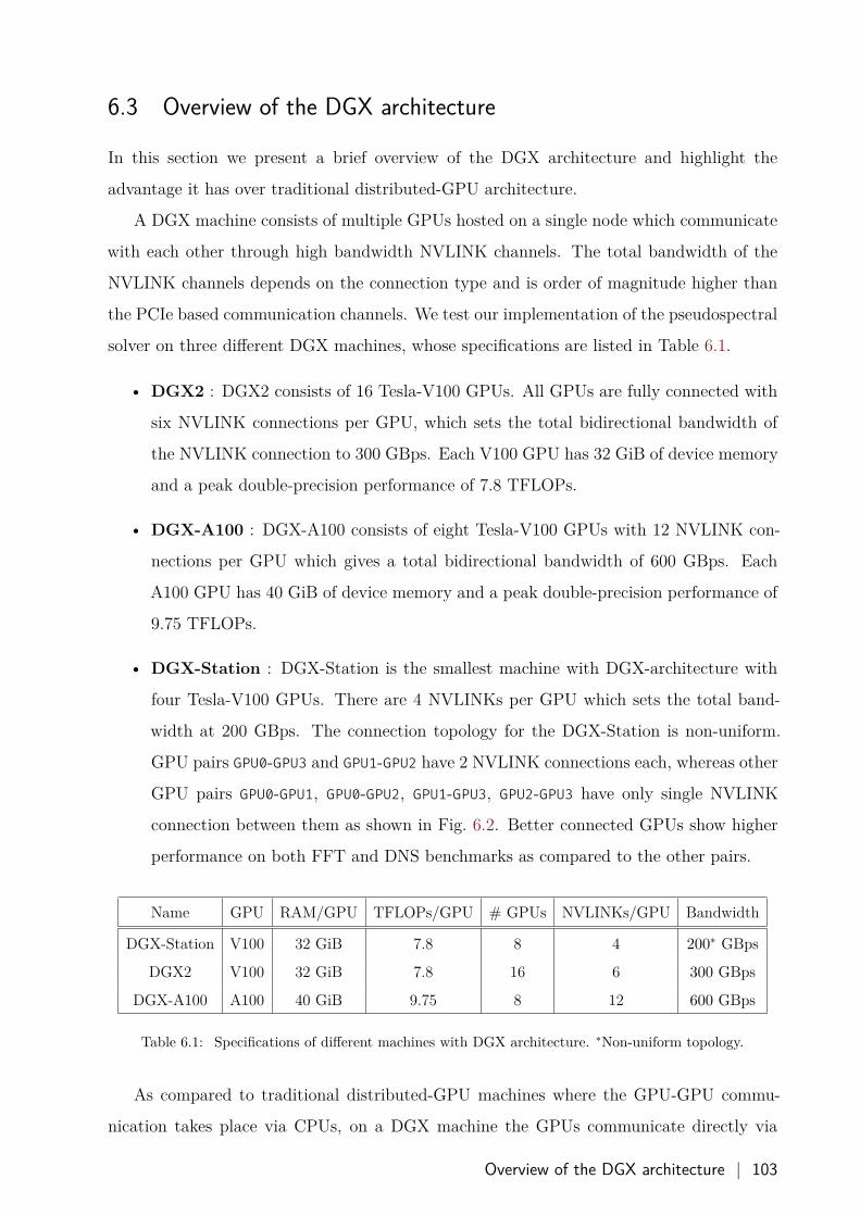
6.3 Overview of the DGX architecture
In this section we present a brief overview of the DGX architecture and highlight the
advantage it has over traditional distributed-GPU architecture.
A DGX machine consists of multiple GPUs hosted on a single node which communicate
with each other through high bandwidth NVLINK channels. The total bandwidth of the
NVLINK channels depends on the connection type and is order of magnitude higher than
the PCIe based communication channels. We test our implementation of the pseudospectral
solver on three different DGX machines, whose specifications are listed in Table 6.1.
• DGX2 : DGX2 consists of 16 Tesla-V100 GPUs. All GPUs are fully connected with
six NVLINK connections per GPU, which sets the total bidirectional bandwidth of
the NVLINK connection to 300 GBps. Each V100 GPU has 32 GiB of device memory
and a peak double-precision performance of 7.8 TFLOPs.
• DGX-A100 : DGX-A100 consists of eight Tesla-V100 GPUs with 12 NVLINK con-
nections per GPU which gives a total bidirectional bandwidth of 600 GBps. Each
A100 GPU has 40 GiB of device memory and a peak double-precision performance of
9.75 TFLOPs.
• DGX-Station : DGX-Station is the smallest machine with DGX-architecture with
four Tesla-V100 GPUs. There are 4 NVLINKs per GPU which sets the total band-
width at 200 GBps. The connection topology for the DGX-Station is non-uniform.
GPU pairs GPU0-GPU3 and GPU1-GPU2 have 2 NVLINK connections each, whereas other
GPU pairs GPU0-GPU1, GPU0-GPU2, GPU1-GPU3, GPU2-GPU3 have only single NVLINK
connection between them as shown in Fig. 6.2. Better connected GPUs show higher
performance on both FFT and DNS benchmarks as compared to the other pairs.
Name GPU RAM/GPU TFLOPs/GPU # GPUs NVLINKs/GPU Bandwidth
DGX-Station V100 32 GiB 7.8 8 4 200∗ GBps
DGX2 V100 32 GiB 7.8 16 6 300 GBps
DGX-A100 A100 40 GiB 9.75 8 12 600 GBps
Table 6.1: Specifications of different machines with DGX architecture. ∗Non-uniform topology.
As compared to traditional distributed-GPU machines where the GPU-GPU commu-
nication takes place via CPUs, on a DGX machine the GPUs communicate directly via
Overview of the DGX architecture | 103
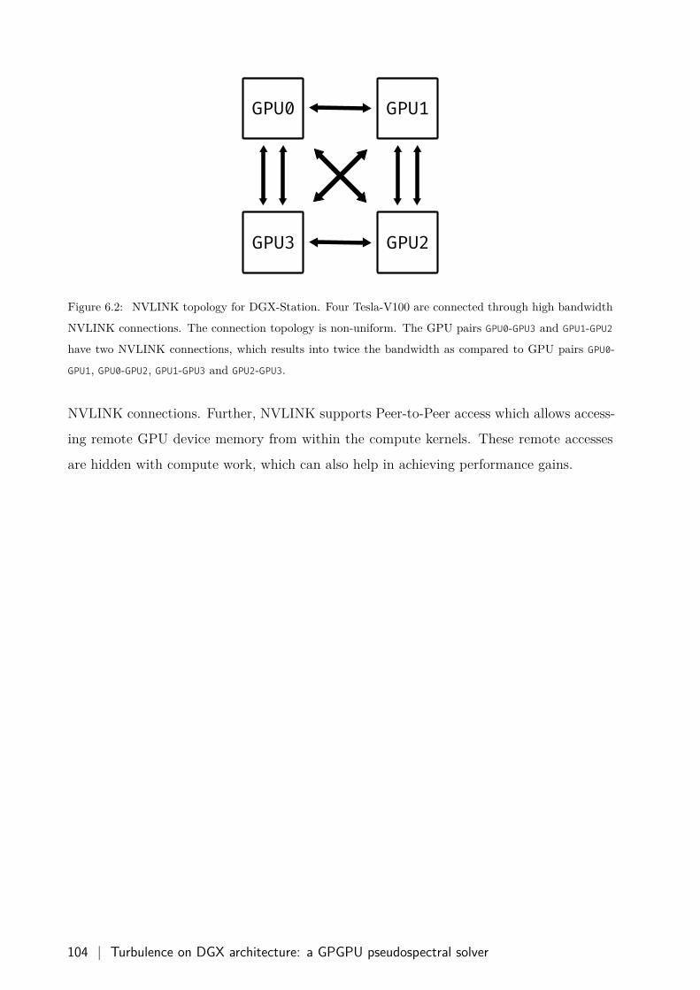
GPU0 GPU1
GPU3 GPU2
Figure 6.2: NVLINK topology for DGX-Station. Four Tesla-V100 are connected through high bandwidth
NVLINK connections. The connection topology is non-uniform. The GPU pairs GPU0-GPU3 and GPU1-GPU2
have two NVLINK connections, which results into twice the bandwidth as compared to GPU pairs GPU0-
GPU1, GPU0-GPU2, GPU1-GPU3 and GPU2-GPU3.
NVLINK connections. Further, NVLINK supports Peer-to-Peer access which allows access-
ing remote GPU device memory from within the compute kernels. These remote accesses
are hidden with compute work, which can also help in achieving performance gains.
104 | Turbulence on DGX architecture: a GPGPU pseudospectral solver
6.4 Earlier attempts on porting FFT algorithms to multi-GPU archi-
tecture
Earlier works have implemented distributed FFT on CUDA enabled GPUs [197–199] but
with poor performance. Nukada et al. [197] show scaling results for up to 768 M2050 Fermi
GPUs for a 20483 size transform using a self-written CUDA FFT implementation. They
achieved a maximum performance which was around 1.2% of the peak performance.
Czechowski et al. [198] designed diGPUFFT which is based on P3DFFT. Although the
library was designed for the experimental validation of theoretical complexity analysis of
three-dimensional FFTs and what implications it has on the design of high performance
exa-scale architectures, once again the authors report a maximum performance which is
less than 1% of the peak performance.
Gholami et al. [199] used both cuFFT and FFTW to compute Fourier transforms on
machines with multiple GPUs distributed across various nodes. The authors were able
to reduce the PCIe communication overhead with novel transpose techniques, but even
with reduced communications, their scaling results show that to offset the communication
overhead incurred while moving from a single GPU to many, one needs a large number of
GPUs to achieve performance similar to a single GPU. Specifically they show that for a
transform of size 256 × 515 × 1024, minimum eight K40 GPUs are required to achieve a
performance comparable to a single K40 GPU.
The common thread in all these earlier studies is the severe communication bottlenecks.
Since the GPUs on different nodes communicate to each other through CPUs, communica-
tion time makes up for more than 70 − 80% of the total execution time, which results in
poor performance.
In the following sections we will show how DGX architecture overcomes these challenges
and is able to deliver a maximum performance for FFT and DNS simulations which is
15 − 20% of the peak performance.
Earlier attempts on porting FFT algorithms to multi-GPU architecture | 105
6.5 Pseudospectral algorithm on the DGX architecture
We now describe the implementation of the pseudospectral solver for the Navier-Stokes
equation for DGX architecture. The solver is written in cudafortran dialect of the Fortran
language. It has two core components:
• The FFT Core, where we define easy to use wrapper functions to perform multi-GPU
FFTs of three dimensional data using the cuFFT library.
• The Pseudospectral Core, which leverages the FFT core to numerically integrate the
Navier-Stokes equation.
Apart from these two core components, our solver contains multi-gpu finite difference
routines which we have used to perform three-dimensional simulations discussed in Chap-
ter 4 . It also contains various analysis routines that can compute common physical quan-
tities like total energy, energy spectrum, energy budget, and handles input and output of
data.
6.6 The FFT Core
We use the cuFFT library to compute Fourier transforms. Specifically, we use the multi-
GPU, in place “Real-to-Complex” (forward) and “Complex-to-Real” (backward) transform
methods, which overwrite the input array with the transformed data. Using in place trans-
form methods helps us to reduce the memory requirements, which can become large very
quickly in three dimensions. See Section 6.9 for the memory requirements for pseudospectral
methods.
6.6.1 Data Layout for the in place transforms
Data layout for the in place cuFFT transforms is determined as follows. We discretize the
velocity field on a cubic box of side length 𝐿 with 𝑁3 collocation points. Wavevectors
available on this domain have components 𝑘𝛼 = 2𝜋𝐿 {−𝑁
2 + 1, −𝑁2 + 2, … , 𝑁
2 − 1, 𝑁2 }. As
the velocity is a real physical variable, its Fourier amplitudes satisfy the Hermitian property
��−𝐤 = ��∗𝐤,
where ��−𝐤 is the complex conjugate of ��𝐤. Thus we only need to store amplitudes for half
the total possible modes, which amounts to storing (𝑁/2+1)𝑁2 complex numbers. Since a
106 | Turbulence on DGX architecture: a GPGPU pseudospectral solver
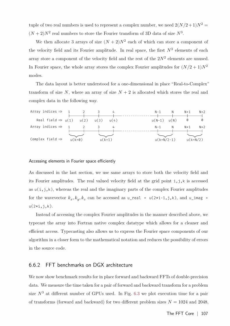
tuple of two real numbers is used to represent a complex number, we need 2(𝑁/2+1)𝑁2 =(𝑁 + 2)𝑁2 real numbers to store the Fourier transform of 3D data of size 𝑁3.
We then allocate 3 arrays of size (𝑁 + 2)𝑁2 each of which can store a component of
the velocity field and its Fourier amplitude. In real space, the first 𝑁3 elements of each
array store a component of the velocity field and the rest of the 2𝑁2 elements are unused.
In Fourier space, the whole array stores the complex Fourier amplitudes for (𝑁/2 + 1)𝑁2
modes.
The data layout is better understood for a one-dimensional in place “Real-to-Complex”
transform of size 𝑁 , where an array of size 𝑁 + 2 is allocated which stores the real and
complex data in the following way.
1 2 3 4
u(1) u(2) u(3) u(4) u(N-1) u(N) 0 0
N-1 N N+1 N+2Array indices ⇒
Real field ⇒1 2 3 4 N-1 N N+1 N+2
u(k=0) u(k=1) u(k=N/2-1) u(k=N/2)
Array indices ⇒
Complex field ⇒
Accessing elements in Fourier space efficiently
As discussed in the last section, we use same arrays to store both the velocity field and
its Fourier amplitudes. The real valued velocity field at the grid point i,j,k is accessed
as u(i,j,k), whereas the real and the imaginary parts of the complex Fourier amplitudes
for the wavevector 𝑘𝑥, 𝑘𝑦, 𝑘𝑧 can be accessed as u_real = u(2*i-1,j,k), and u_imag =
u(2*i,j,k).
Instead of accessing the complex Fourier amplitudes in the manner described above, we
typecast the array into Fortran native complex datatype which allows for a cleaner and
efficient access. Typecasting also allows us to express the Fourier space components of our
algorithm in a closer form to the mathematical notation and reduces the possibility of errors
in the source code.
6.6.2 FFT benchmarks on DGX architecture
We now show benchmark results for in place forward and backward FFTs of double-precision
data. We measure the time taken for a pair of forward and backward transform for a problem
size 𝑁3 at different number of GPUs used. In Fig. 6.3 we plot execution time for a pair
of transforms (forward and backward) for two different problem sizes 𝑁 = 1024 and 2048,
The FFT Core | 107
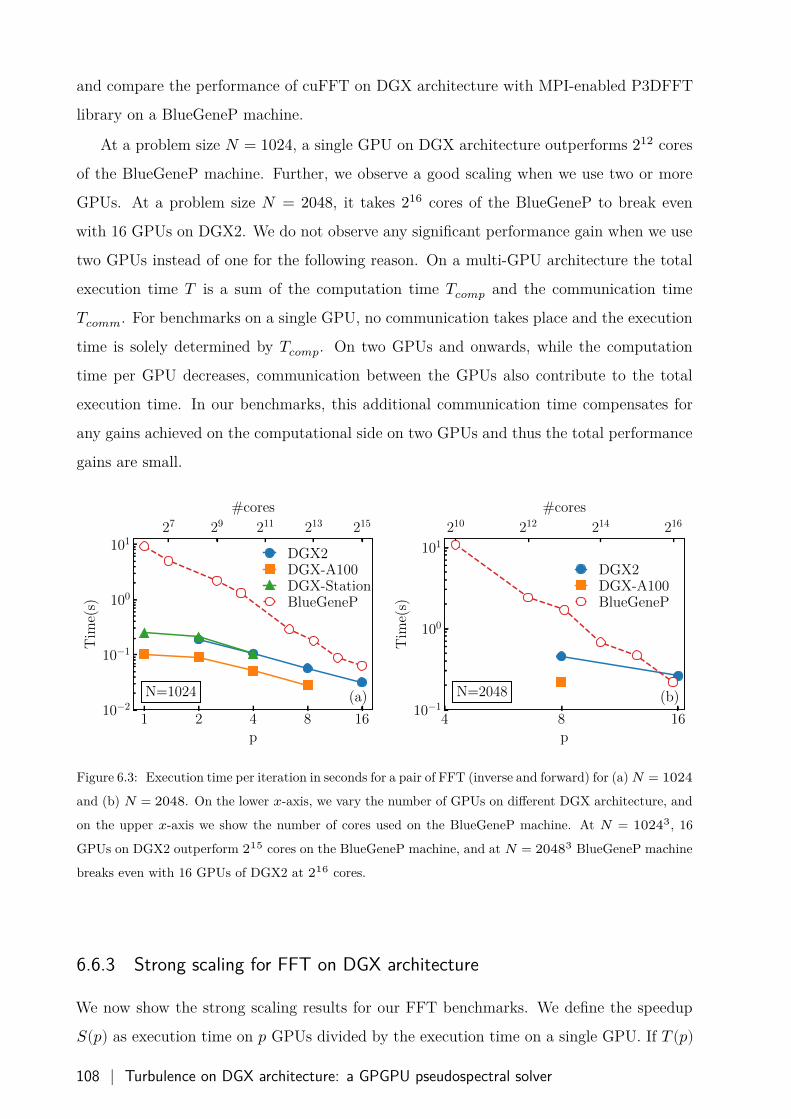
and compare the performance of cuFFT on DGX architecture with MPI-enabled P3DFFT
library on a BlueGeneP machine.
At a problem size 𝑁 = 1024, a single GPU on DGX architecture outperforms 212 cores
of the BlueGeneP machine. Further, we observe a good scaling when we use two or more
GPUs. At a problem size 𝑁 = 2048, it takes 216 cores of the BlueGeneP to break even
with 16 GPUs on DGX2. We do not observe any significant performance gain when we use
two GPUs instead of one for the following reason. On a multi-GPU architecture the total
execution time 𝑇 is a sum of the computation time 𝑇𝑐𝑜𝑚𝑝 and the communication time
𝑇𝑐𝑜𝑚𝑚. For benchmarks on a single GPU, no communication takes place and the execution
time is solely determined by 𝑇𝑐𝑜𝑚𝑝. On two GPUs and onwards, while the computation
time per GPU decreases, communication between the GPUs also contribute to the total
execution time. In our benchmarks, this additional communication time compensates for
any gains achieved on the computational side on two GPUs and thus the total performance
gains are small.
1 2 4 8 16p
10−2
10−1
100
101
Tim
e(s)
N=1024 (a)
DGX2DGX-A100DGX-StationBlueGeneP
4 8 16p
10−1
100
101
Tim
e(s)
N=2048 (b)
DGX2DGX-A100BlueGeneP
27 29 211 213 215
#cores
210 212 214 216
#cores
Figure 6.3: Execution time per iteration in seconds for a pair of FFT (inverse and forward) for (a) 𝑁 = 1024and (b) 𝑁 = 2048. On the lower 𝑥-axis, we vary the number of GPUs on different DGX architecture, and
on the upper 𝑥-axis we show the number of cores used on the BlueGeneP machine. At 𝑁 = 10243, 16
GPUs on DGX2 outperform 215 cores on the BlueGeneP machine, and at 𝑁 = 20483 BlueGeneP machine
breaks even with 16 GPUs of DGX2 at 216 cores.
6.6.3 Strong scaling for FFT on DGX architecture
We now show the strong scaling results for our FFT benchmarks. We define the speedup
𝑆(𝑝) as execution time on 𝑝 GPUs divided by the execution time on a single GPU. If 𝑇 (𝑝)
108 | Turbulence on DGX architecture: a GPGPU pseudospectral solver
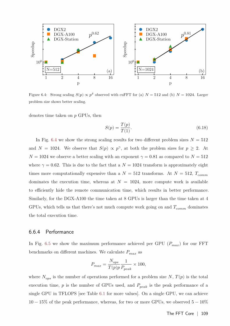
1 2 4 8 16p
100
Sp
eed
up
p0.62
N=512 (a)
DGX2DGX-A100DGX-Station
1 2 4 8 16p
100
Sp
eed
up
p0.81
N=1024 (b)
DGX2DGX-A100DGX-Station
Figure 6.4: Strong scaling 𝑆(𝑝) ∝ 𝑝𝛿 observed with cuFFT for (a) 𝑁 = 512 and (b) 𝑁 = 1024. Larger
problem size shows better scaling.
denotes time taken on 𝑝 GPUs, then
𝑆(𝑝) = 𝑇 (𝑝)𝑇 (1) . (6.18)
In Fig. 6.4 we show the strong scaling results for two different problem sizes 𝑁 = 512and 𝑁 = 1024. We observe that 𝑆(𝑝) ∝ 𝑝𝛾, at both the problem sizes for 𝑝 ≥ 2. At
𝑁 = 1024 we observe a better scaling with an exponent 𝛾 = 0.81 as compared to 𝑁 = 512where 𝛾 = 0.62. This is due to the fact that a 𝑁 = 1024 transform is approximately eight
times more computationally expensive than a 𝑁 = 512 transforms. At 𝑁 = 512, 𝑇𝑐𝑜𝑚𝑚
dominates the execution time, whereas at 𝑁 = 1024, more compute work is available
to efficiently hide the remote communication time, which results in better performance.
Similarly, for the DGX-A100 the time taken at 8 GPUs is larger than the time taken at 4
GPUs, which tells us that there’s not much compute work going on and 𝑇𝑐𝑜𝑚𝑚 dominates
the total execution time.
6.6.4 Performance
In Fig. 6.5 we show the maximum performance achieved per GPU (𝑃𝑚𝑎𝑥) for our FFT
benchmarks on different machines. We calculate 𝑃𝑚𝑎𝑥 as
𝑃𝑚𝑎𝑥 = 𝑁𝑜𝑝𝑠𝑇 (𝑝)𝑝
1𝑃𝑝𝑒𝑎𝑘
× 100,
where 𝑁𝑜𝑝𝑠 is the number of operations performed for a problem size 𝑁 , 𝑇 (𝑝) is the total
execution time, 𝑝 is the number of GPUs used, and 𝑃𝑝𝑒𝑎𝑘 is the peak performance of a
single GPU in TFLOPS [see Table 6.1 for more values]. On a single GPU, we can achieve
10 − 15% of the peak performance, whereas, for two or more GPUs, we observed 5 − 10%
The FFT Core | 109
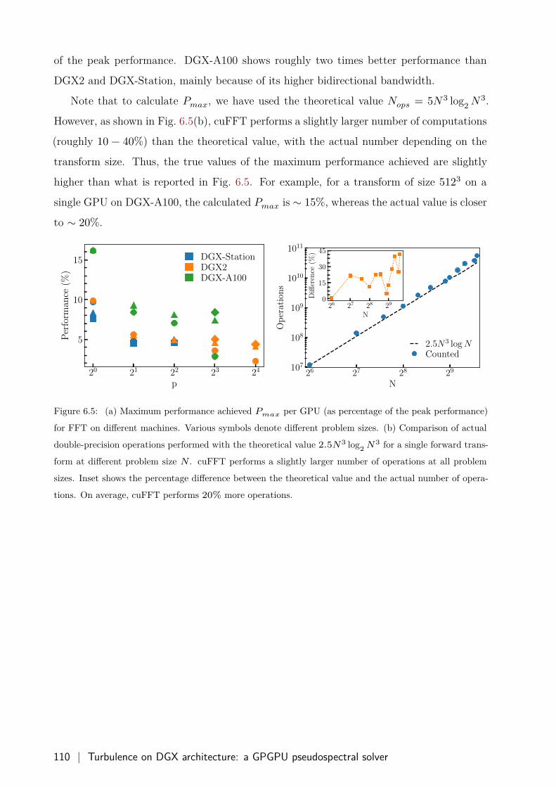
of the peak performance. DGX-A100 shows roughly two times better performance than
DGX2 and DGX-Station, mainly because of its higher bidirectional bandwidth.
Note that to calculate 𝑃𝑚𝑎𝑥, we have used the theoretical value 𝑁𝑜𝑝𝑠 = 5𝑁3 log2 𝑁3.
However, as shown in Fig. 6.5(b), cuFFT performs a slightly larger number of computations
(roughly 10 − 40%) than the theoretical value, with the actual number depending on the
transform size. Thus, the true values of the maximum performance achieved are slightly
higher than what is reported in Fig. 6.5. For example, for a transform of size 5123 on a
single GPU on DGX-A100, the calculated 𝑃𝑚𝑎𝑥 is ∼ 15%, whereas the actual value is closer
to ∼ 20%.
20 21 22 23 24
p
5
10
15
Per
form
ance
(%)
DGX-StationDGX2DGX-A100
26 27 28 29
N
107
108
109
1010
1011
Op
erat
ion
s
26 27 28 29
N
0
15
30
45
Diff
eren
ce(%
)
2.5N3 logNCounted
Figure 6.5: (a) Maximum performance achieved 𝑃𝑚𝑎𝑥 per GPU (as percentage of the peak performance)
for FFT on different machines. Various symbols denote different problem sizes. (b) Comparison of actual
double-precision operations performed with the theoretical value 2.5𝑁3 log2 𝑁3 for a single forward trans-
form at different problem size 𝑁. cuFFT performs a slightly larger number of operations at all problem
sizes. Inset shows the percentage difference between the theoretical value and the actual number of opera-
tions. On average, cuFFT performs 20% more operations.
110 | Turbulence on DGX architecture: a GPGPU pseudospectral solver
6.7 The Pseudospectral Core
We now describe the different steps of our GPGPU implementation of the pseudospectral
algorithm.
1. Initialization : The simulation is setup here. Required array are allocated, initial
conditions are set and ETD integration factors are computed.
2. Velocity in the Fourier space : Beginning of the time loop. If the velocity field was
initialized in real space, it is transformed to Fourier space before proceeding further.
3. Spectral analysis (Optional) : As the velocity is in Fourier space, spectral analysis,
for example, calculation of the energy spectrum is carried out at this step.
4. To real space : The velocity and vorticity arrays are transformed back to the real
space.
5. Real analysis, Snapshots (Optional): The velocity and vorticity fields are in real space
at this time step, and any real space analysis is performed here. Additionally, snap-
shots of the velocity field are also stored.
6. Compute the nonlinear term: Nonlinear term is computed and stored in the array
containing the vorticity field.
7. Add real space forces (Optional): Any additional forcing terms, which are better rep-
resented in the real space are added to the array containing the nonlinear term at this
step.
8. To Fourier space: The array containing the nonlinear term and additional real space
forces is transformed to the Fourier space.
9. Add Fourier space forces (Optional): Any additional forcing terms, which are better
represented in the Fourier space are added to the array containing the nonlinear term
at this step.
10. Integration: Time integration is performed at this step.
First, we apply the projection operator on the array containing the nonlinear term
and additional forces to get 𝐹𝐤(𝑡), and then the velocity is updated appropriately.
Additionally, 𝐹𝐤(𝑡) is stored away for use in the next integration time step. At this
The Pseudospectral Core | 111
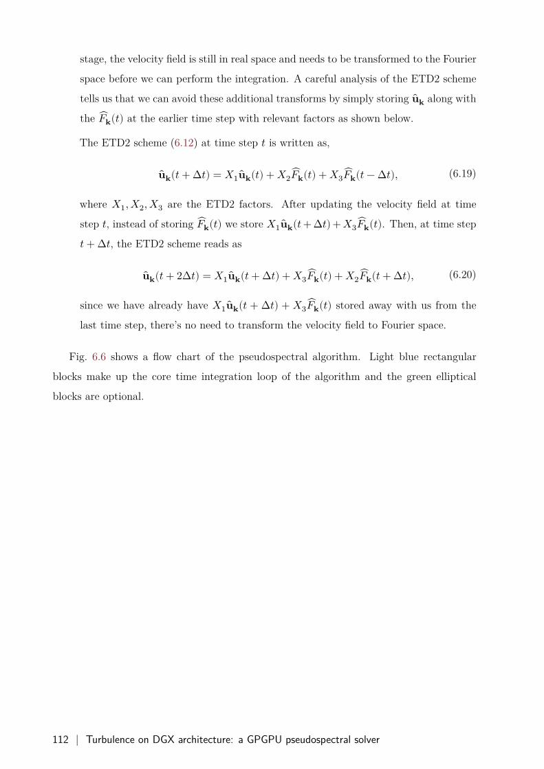
stage, the velocity field is still in real space and needs to be transformed to the Fourier
space before we can perform the integration. A careful analysis of the ETD2 scheme
tells us that we can avoid these additional transforms by simply storing ��𝐤 along with
the 𝐹𝐤(𝑡) at the earlier time step with relevant factors as shown below.
The ETD2 scheme (6.12) at time step 𝑡 is written as,
��𝐤(𝑡 + Δ𝑡) = 𝑋1��𝐤(𝑡) + 𝑋2𝐹𝐤(𝑡) + 𝑋3𝐹𝐤(𝑡 − Δ𝑡), (6.19)
where 𝑋1, 𝑋2, 𝑋3 are the ETD2 factors. After updating the velocity field at time
step 𝑡, instead of storing 𝐹𝐤(𝑡) we store 𝑋1��𝐤(𝑡 + Δ𝑡) + 𝑋3𝐹𝐤(𝑡). Then, at time step
𝑡 + Δ𝑡, the ETD2 scheme reads as
��𝐤(𝑡 + 2Δ𝑡) = 𝑋1��𝐤(𝑡 + Δ𝑡) + 𝑋3𝐹𝐤(𝑡) + 𝑋2𝐹𝐤(𝑡 + Δ𝑡), (6.20)
since we have already have 𝑋1��𝐤(𝑡 + Δ𝑡) + 𝑋3𝐹𝐤(𝑡) stored away with us from the
last time step, there’s no need to transform the velocity field to Fourier space.
Fig. 6.6 shows a flow chart of the pseudospectral algorithm. Light blue rectangular
blocks make up the core time integration loop of the algorithm and the green elliptical
blocks are optional.
112 | Turbulence on DGX architecture: a GPGPU pseudospectral solver
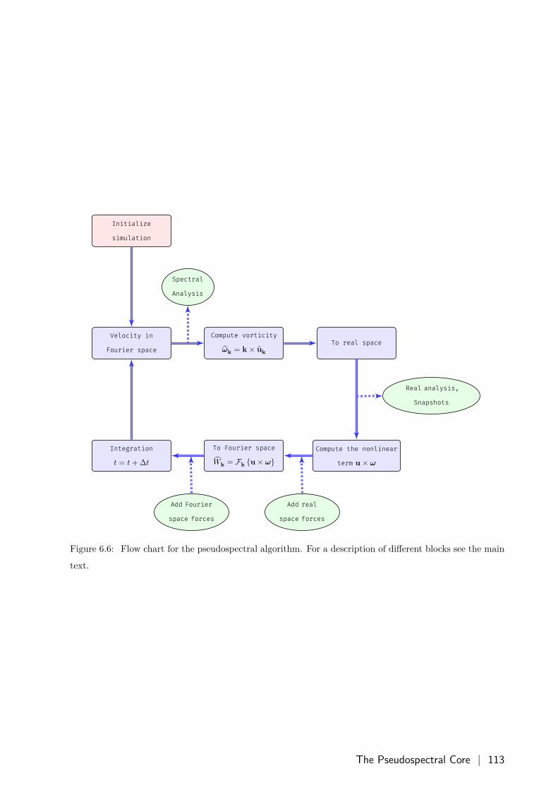
Initialize
simulation
Velocity in
Fourier space
Compute vorticity
𝝎𝐤 = 𝐤 × ��𝐤To real space
Compute the nonlinear
term 𝐮 × 𝝎To Fourier space
𝑊𝐤 = F𝐤 {𝐮 × 𝝎}Integration
𝑡 = 𝑡 + Δ𝑡
Spectral
Analysis
Real analysis,
Snapshots
Add real
space forces
Add Fourier
space forces
Figure 6.6: Flow chart for the pseudospectral algorithm. For a description of different blocks see the main
text.
The Pseudospectral Core | 113
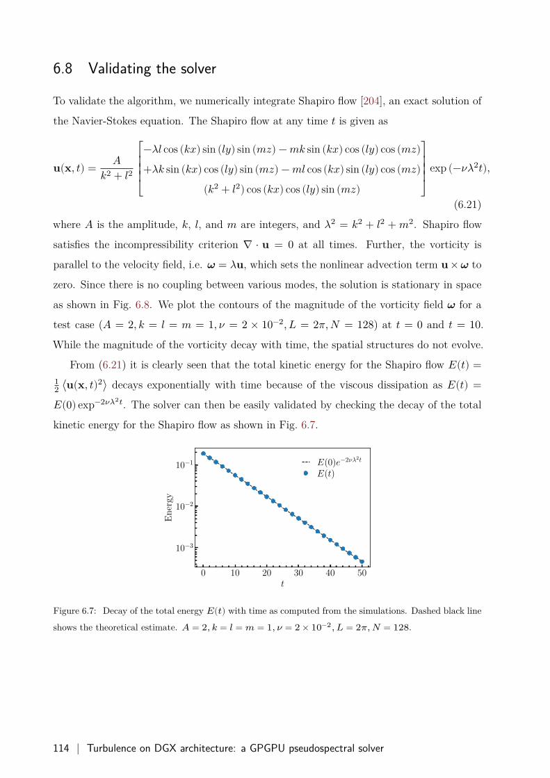
6.8 Validating the solver
To validate the algorithm, we numerically integrate Shapiro flow [204], an exact solution of
the Navier-Stokes equation. The Shapiro flow at any time 𝑡 is given as
𝐮(𝐱, 𝑡) = 𝐴𝑘2 + 𝑙2
⎡⎢⎢⎢⎣
−𝜆𝑙 cos (𝑘𝑥) sin (𝑙𝑦) sin (𝑚𝑧) − 𝑚𝑘 sin (𝑘𝑥) cos (𝑙𝑦) cos (𝑚𝑧)+𝜆𝑘 sin (𝑘𝑥) cos (𝑙𝑦) sin (𝑚𝑧) − 𝑚𝑙 cos (𝑘𝑥) sin (𝑙𝑦) cos (𝑚𝑧)
(𝑘2 + 𝑙2) cos (𝑘𝑥) cos (𝑙𝑦) sin (𝑚𝑧)
⎤⎥⎥⎥⎦
exp (−𝜈𝜆2𝑡),
(6.21)
where 𝐴 is the amplitude, 𝑘, 𝑙, and 𝑚 are integers, and 𝜆2 = 𝑘2 + 𝑙2 + 𝑚2. Shapiro flow
satisfies the incompressibility criterion ∇ ⋅ 𝐮 = 0 at all times. Further, the vorticity is
parallel to the velocity field, i.e. 𝝎 = 𝜆𝐮, which sets the nonlinear advection term 𝐮 × 𝝎 to
zero. Since there is no coupling between various modes, the solution is stationary in space
as shown in Fig. 6.8. We plot the contours of the magnitude of the vorticity field 𝝎 for a
test case (𝐴 = 2, 𝑘 = 𝑙 = 𝑚 = 1, 𝜈 = 2 × 10⁻², 𝐿 = 2𝜋, 𝑁 = 128) at 𝑡 = 0 and 𝑡 = 10.
While the magnitude of the vorticity decay with time, the spatial structures do not evolve.
From (6.21) it is clearly seen that the total kinetic energy for the Shapiro flow 𝐸(𝑡) =12 ⟨𝐮(𝐱, 𝑡)2⟩ decays exponentially with time because of the viscous dissipation as 𝐸(𝑡) =𝐸(0) exp−2𝜈𝜆2𝑡. The solver can then be easily validated by checking the decay of the total
kinetic energy for the Shapiro flow as shown in Fig. 6.7.
0 10 20 30 40 50t
10−3
10−2
10−1
En
ergy
E(0)e−2νλ2t
E(t)
Figure 6.7: Decay of the total energy 𝐸(𝑡) with time as computed from the simulations. Dashed black line
shows the theoretical estimate. 𝐴 = 2, 𝑘 = 𝑙 = 𝑚 = 1, 𝜈 = 2 × 10⁻², 𝐿 = 2𝜋, 𝑁 = 128.
114 | Turbulence on DGX architecture: a GPGPU pseudospectral solver
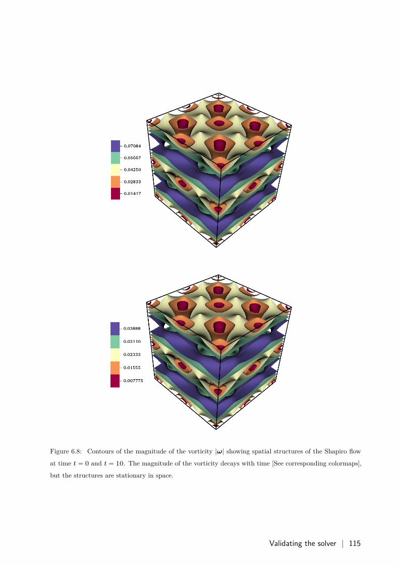
Figure 6.8: Contours of the magnitude of the vorticity |𝝎| showing spatial structures of the Shapiro flow
at time 𝑡 = 0 and 𝑡 = 10. The magnitude of the vorticity decays with time [See corresponding colormaps],
but the structures are stationary in space.
Validating the solver | 115
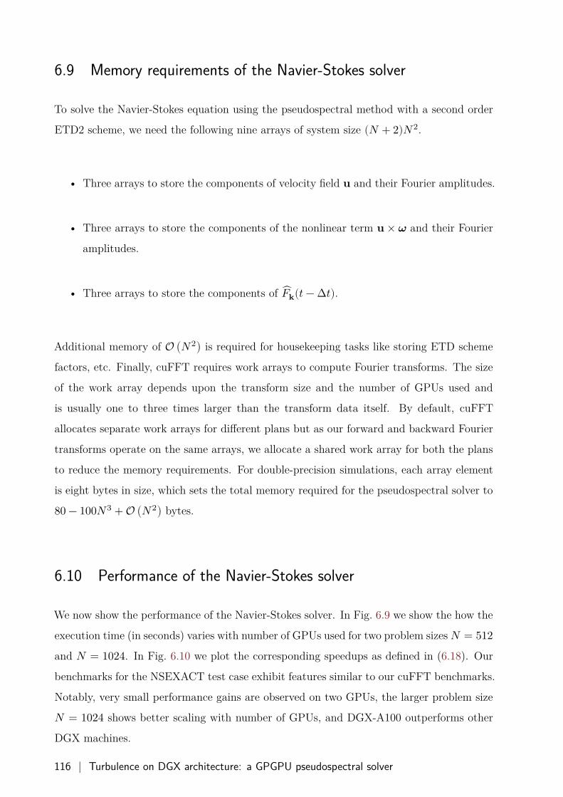
6.9 Memory requirements of the Navier-Stokes solver
To solve the Navier-Stokes equation using the pseudospectral method with a second order
ETD2 scheme, we need the following nine arrays of system size (𝑁 + 2)𝑁2.
• Three arrays to store the components of velocity field 𝐮 and their Fourier amplitudes.
• Three arrays to store the components of the nonlinear term 𝐮 × 𝝎 and their Fourier
amplitudes.
• Three arrays to store the components of 𝐹𝐤(𝑡 − Δ𝑡).
Additional memory of O (𝑁2) is required for housekeeping tasks like storing ETD scheme
factors, etc. Finally, cuFFT requires work arrays to compute Fourier transforms. The size
of the work array depends upon the transform size and the number of GPUs used and
is usually one to three times larger than the transform data itself. By default, cuFFT
allocates separate work arrays for different plans but as our forward and backward Fourier
transforms operate on the same arrays, we allocate a shared work array for both the plans
to reduce the memory requirements. For double-precision simulations, each array element
is eight bytes in size, which sets the total memory required for the pseudospectral solver to
80 − 100𝑁3 + O (𝑁2) bytes.
6.10 Performance of the Navier-Stokes solver
We now show the performance of the Navier-Stokes solver. In Fig. 6.9 we show the how the
execution time (in seconds) varies with number of GPUs used for two problem sizes 𝑁 = 512and 𝑁 = 1024. In Fig. 6.10 we plot the corresponding speedups as defined in (6.18). Our
benchmarks for the NSEXACT test case exhibit features similar to our cuFFT benchmarks.
Notably, very small performance gains are observed on two GPUs, the larger problem size
𝑁 = 1024 shows better scaling with number of GPUs, and DGX-A100 outperforms other
DGX machines.
116 | Turbulence on DGX architecture: a GPGPU pseudospectral solver
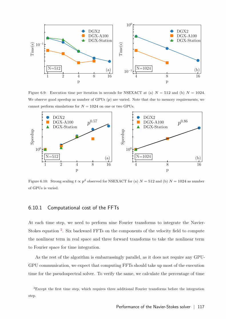
1 2 4 8 16p
10−1
Tim
e(s)
N=512 (a)
DGX2DGX-A100DGX-Station
4 8 16p
10−1
100
Tim
e(s)
N=1024 (b)
DGX2DGX-A100DGX-Station
Figure 6.9: Execution time per iteration in seconds for NSEXACT at (a) 𝑁 = 512 and (b) 𝑁 = 1024.
We observe good speedup as number of GPUs (𝑝) are varied. Note that due to memory requirements, we
cannot perform simulations for 𝑁 = 1024 on one or two GPUs.
1 2 4 8 16p
100
Sp
eed
up
p0.57
N=512 (a)
DGX2DGX-A100DGX-Station
4 8 16p
100
Sp
eed
up
p0.86
N=1024 (b)
DGX2DGX-A100DGX-Station
Figure 6.10: Strong scaling 𝑡 ∝ 𝑝𝛿 observed for NSEXACT for (a) 𝑁 = 512 and (b) 𝑁 = 1024 as number
of GPUs is varied.
6.10.1 Computational cost of the FFTs
At each time step, we need to perform nine Fourier transforms to integrate the Navier-
Stokes equation 2. Six backward FFTs on the components of the velocity field to compute
the nonlinear term in real space and three forward transforms to take the nonlinear term
to Fourier space for time integration.
As the rest of the algorithm is embarrassingly parallel, as it does not require any GPU-
GPU communication, we expect that computing FFTs should take up most of the execution
time for the pseudospectral solver. To verify the same, we calculate the percentage of time
2Except the first time step, which requires three additional Fourier transforms before the integration
step.
Performance of the Navier-Stokes solver | 117
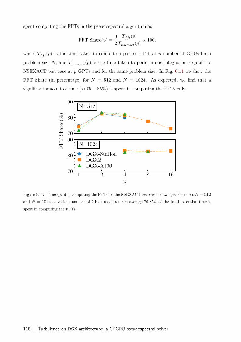
spent computing the FFTs in the pseudospectral algorithm as
FFT Share(p) = 92
𝑇𝑓𝑓𝑡(𝑝)𝑇𝑛𝑠𝑒𝑥𝑎𝑐𝑡(𝑝) × 100,
where 𝑇𝑓𝑓𝑡(𝑝) is the time taken to compute a pair of FFTs at 𝑝 number of GPUs for a
problem size 𝑁 , and 𝑇𝑛𝑠𝑒𝑥𝑎𝑐𝑡(𝑝) is the time taken to perform one integration step of the
NSEXACT test case at 𝑝 GPUs and for the same problem size. In Fig. 6.11 we show the
FFT Share (in percentage) for 𝑁 = 512 and 𝑁 = 1024. As expected, we find that a
significant amount of time (≈ 75 − 85%) is spent in computing the FFTs only.
70
80
90N=512
1 2 4 8 16p
70
80
90N=1024
FF
TS
har
e(%
)
DGX-StationDGX2DGX-A100
Figure 6.11: Time spent in computing the FFTs for the NSEXACT test case for two problem sizes 𝑁 = 512and 𝑁 = 1024 at various number of GPUs used (𝑝). On average 70-85% of the total execution time is
spent in computing the FFTs.
118 | Turbulence on DGX architecture: a GPGPU pseudospectral solver
6.11 Limitations of the GPGPU solver
As we have shown in this chapter, pseudospectral algorithms perform well on DGX architec-
ture, which, owing to its powerful GPU cards and high bandwidth NVLINK communication
channels, is an ideal platform for performing moderate resolution DNS (5123 − 20483) of
the Navier-Stokes equation. However, there are some limitations of using pseudospectral
algorithms on DGX architecture, which we address now.
• Architecture specific: The current implementation of our solver is specific to DGX-
architecture only, where multiple GPUs reside on a single node and communicate via
NVLINK communication. With few tweaks, the implementation should also work
on multiple GPUs without NVLINK support, but the performance gains rely heav-
ily on the high-speed communication channels between the GPUs. Further, GPUs
distributed over multiple nodes are not supported yet.
• Memory requirements: As discussed earlier, the total memory required to perform a
simulation at a 𝑁3 resolution is around 80−100𝑁3 +O (𝑁2) bytes. For example, for
the NSEXACT test case at 𝑁3 = 10243 resolution, around 90 GiB of device memory
is required. A single Tesla-V100 has 32 GiB device memory, and we need four such
GPUs to perform the simulations at this resolution. Often, the fluid flow is coupled
with other physical fields, in which case memory requirements can increase two or
three-folds, which severely reduces the maximum achievable resolution. For example,
in wet incompressible polar active runs performed in Chapter 4, we need 18 additional
system size arrays, which brings the total memory requirements to 220−240𝑁3 bytes.
For these simulations, the maximum resolution we can achieve on DGX-Station then
reduces to 𝑁3 = 5123.
• Ease of development: While multiple libraries are available for CUDA programming
in C/C++, the support for cudafortran is not as extensive. The situation is improv-
ing rapidly, and one can still use the Fortran-C bindings to write wrappers for any
C/C++ libraries which are not available in cudafortran. Although it is doable, it
does introduce some friction and is not suitable for beginners. In addition, some al-
gorithms are easier to write on CPUs and require extensive efforts to port them over
to GPUs. OpenACC standard attempts to alleviate these issues and is designed to
simplify parallel programming of heterogeneous CPU/GPU systems.
Limitations of the GPGPU solver | 119
6.12 Conclusions and future work
Regardless of the limitations mentioned above, GPGPU pseudospectral methods show ex-
cellent performance and strong scaling as we increase the number of GPUs used on DGX
architecture. Thus, DGX architecture is an ideal platform to perform the DNS of the
Navier-Stokes equation on moderate resolutions of 5123 − 20483. The algorithm can be
easily ported to two dimensions, where the memory scales with the resolution as O (𝑁2),
and one can achieve very high-resolution simulations viz. 327682 − 655362.
Overall, memory requirements are the major bottleneck to perform high-resolution sim-
ulations in three dimensions. In the future, we will focus on adding support for GPUs
distributed over multiple nodes, which will allow us to achieve higher resolutions but at
the expense of performance. Further, we will couple the pseudospectral solver with particle
tracking methods and mesh evolution algorithms.
120 | Turbulence on DGX architecture: a GPGPU pseudospectral solver
Chapter 7
Conclusions and future directions
In this thesis, we have studied the statistical and dynamical properties of incompressible
polar active matter.
In Chapters 2 and 3 we studied the coarsening dynamics of the ITT equation at various
Re in 2D and 3D, respectively. In particular, we have shown that coarsening proceeds
via repeated defect merger events. In 2D, defects are uniformly distributed at all Re,
and a unique growing length scale characterizes the coarsening dynamics. At low Re, the
coarsening dynamics proceeds similarly to the XY model, whereas at high Re, we observed a
forward enstrophy cascade and showed that turbulence accelerates the coarsening dynamics.
In 3D, the spatial distribution of defects depends on Re. At low Re, similar to 2D, defects
are uniformly distributed, at high Re we observed defect-clustering in the intense vorticity
regions. We observe Kolmogorov scaling in the energy spectrum over a range of length
scales and a forward energy cascade. While low Re coarsening is governed by a unique
growing length scale, at high Re our structure-function analysis indicates the presence of
multiple interacting length scales.
In our coarsening studies, we have focused on the constant concentration limit. A
straight-forward direction would be to study the coarsening dynamics in the presence of
concentration fluctuations. Indeed, earlier studies [34, 41–43] on the coarsening dynamics
of the Toner-Tu equations with concentration fluctuations have reported that both the
velocity and coarsening fields are coupled and coarsen simultaneously but with different
scaling exponents. Further, the coarsening proceeds faster compared to equilibrium systems.
However, a detailed study of the energy transfer and defect dynamics in systems with
concentration fluctuations is still lacking.
In Chapter 4 we studied dense suspensions of extensile swimmers in two and three
| 121
dimensions. We investigated the instabilities of the aligned state to small perturbations
and established how inertia can stabilize the orientational order. We found that a non
dimensional parameter 𝑅 characterizes the stability of the aligned state. At small 𝑅, the
instabilities in the ordered state exhibit a growth rate proportional to O(𝑞). For 𝑅 > 𝑅1,
the instabilities grow at a rate proportional to O(𝑞2). Past a second threshold 𝑅2, the
flock is stable. Further, we performed high-resolution direct numerical simulations and
characterize the properties of the spatio-temporal chaos arising from the instabilities. We
showed that in two dimensions, for all 𝑅 < 𝑅2, the flow is riddled with topological vortices
with no global order in sight. The correlation length (or the inter-defect spacing) grows with
𝑅 and appears to diverge at 𝑅2. Our preliminary DNS in 3D showed that bulk suspensions
also exhibit defects for 𝑅 < 𝑅2. To characterize the properties of growing inter-defect
separation and the order-disorder transition requires numerical studies on larger system
size, which is another future direction to look forward to.
In Chapter 4 and Chatterjee et al. [55] we have shown that the most unstable modes for
the number-conserving, Malthusian, and dense suspensions are identical, but the statistical
properties of the turbulent states differ widely. For the Malthusian case, we observed an
order-disorder transition from defect-turbulent states to phase-turbulent states at 𝑅 = 𝑅1.
In dense suspensions, defect-turbulent states persist all the way up to 𝑅 = 𝑅2. How
incompressibility suppresses the transition from defect-ridden states to phase-turbulence
is still remains to be addressed. Further, how the inclusion of concentration fluctuations
alters the nature of steady states and the transition remains yet to be studied. We also
look forward to the experimental validation of our linear stability and numerical studies.
In general, in Chapters 2 to 4 we have shown that topological defects play a crucial role
in determining the dynamics of incompressible polar active systems. While much is known
about the nature of topological defects for equilibrium systems, interest in active defects
is relatively new, and much remains unexplored. A recent review article by Shankar et al.
[64] has highlighted the advances in this direction. The complex nonlinear terms in the
equations of dry and wet polar active systems alter the nature of defects. For example, in
the Malthusian suspensions [55], we have shown that due to the presence of self-propulsion
term asters are preferred over spirals and the saddles have string-like structures. Defect
dynamics in active systems is another area of interest.
In Chapter 5 we focused on a colony of nonmotile bacteria growing on a hard agar sur-
face. Here, the activity arises not from the particle motility, but the birth-death processes.
122 | Conclusions and future directions
At the colony front, bacteria repeatedly grow and divide at the expense of nutrients and
push each other in the process. The colony thus expands because of the steric repulsions
between the bacteria. While the interior of the colony is densely populated, population
fluctuations intrinsic to any birth-death process become essential for such systems at the
growing front where the number of organisms is small. We investigated how these fluctua-
tions and nutrient availability can affect the growing colony’s morphology. We found that
the population fluctuations and nutrient-dependent bacteria diffusion are sufficient to cause
a morphological transition from finger-like branched fronts to smooth fronts with increasing
nutrient concentration.
In Chapter 6 we presented a general purpose GPU based (GPGPU) pseudospectral
solver for the Navier-Stokes equation. We showed how the DGX architecture is an ideal
platform to perform discrete numerical simulations of the Navier-Stokes and related equa-
tions at moderate resolutions of size 5123 −20483. Our GPGPU pseudospectral solver in its
current state is designed for multiple GPUs hosted on a single node. To tackle much more
computationally intensive problems, for example the characterization of the order-disorder
transition in wet suspensions in 3D, we plan to support multi-node multi-GPU architecture
in near future.
Finally, we have used coarse-grained hydrodynamic equations in our numerical studies of
incompressible polar active systems. An alternative approach is to use agent-based models
of active systems, where each particle is modelled at the microscopic level. Concentration
fluctuations are intrinsic to these models. For example, the coarsening dynamics described
in Chapter 2 can also be studied with motile rods moving on frictional substrates [165].
| 123

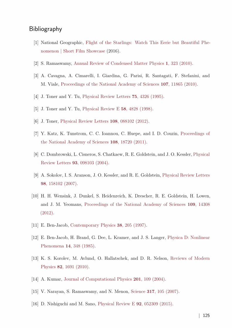
Bibliography
[1] National Geographic, Flight of the Starlings: Watch This Eerie but Beautiful Phe-
nomenon | Short Film Showcase (2016).
[2] S. Ramaswamy, Annual Review of Condensed Matter Physics 1, 323 (2010).
[3] A. Cavagna, A. Cimarelli, I. Giardina, G. Parisi, R. Santagati, F. Stefanini, and
M. Viale, Proceedings of the National Academy of Sciences 107, 11865 (2010).
[4] J. Toner and Y. Tu, Physical Review Letters 75, 4326 (1995).
[5] J. Toner and Y. Tu, Physical Review E 58, 4828 (1998).
[6] J. Toner, Physical Review Letters 108, 088102 (2012).
[7] Y. Katz, K. Tunstrom, C. C. Ioannou, C. Huepe, and I. D. Couzin, Proceedings of
the National Academy of Sciences 108, 18720 (2011).
[8] C. Dombrowski, L. Cisneros, S. Chatkaew, R. E. Goldstein, and J. O. Kessler, Physical
Review Letters 93, 098103 (2004).
[9] A. Sokolov, I. S. Aranson, J. O. Kessler, and R. E. Goldstein, Physical Review Letters
98, 158102 (2007).
[10] H. H. Wensink, J. Dunkel, S. Heidenreich, K. Drescher, R. E. Goldstein, H. Lowen,
and J. M. Yeomans, Proceedings of the National Academy of Sciences 109, 14308
(2012).
[11] E. Ben-Jacob, Contemporary Physics 38, 205 (1997).
[12] E. Ben-Jacob, H. Brand, G. Dee, L. Kramer, and J. S. Langer, Physica D: Nonlinear
Phenomena 14, 348 (1985).
[13] K. S. Korolev, M. Avlund, O. Hallatschek, and D. R. Nelson, Reviews of Modern
Physics 82, 1691 (2010).
[14] A. Kumar, Journal of Computational Physics 201, 109 (2004).
[15] V. Narayan, S. Ramaswamy, and N. Menon, Science 317, 105 (2007).
[16] D. Nishiguchi and M. Sano, Physical Review E 92, 052309 (2015).
| 125
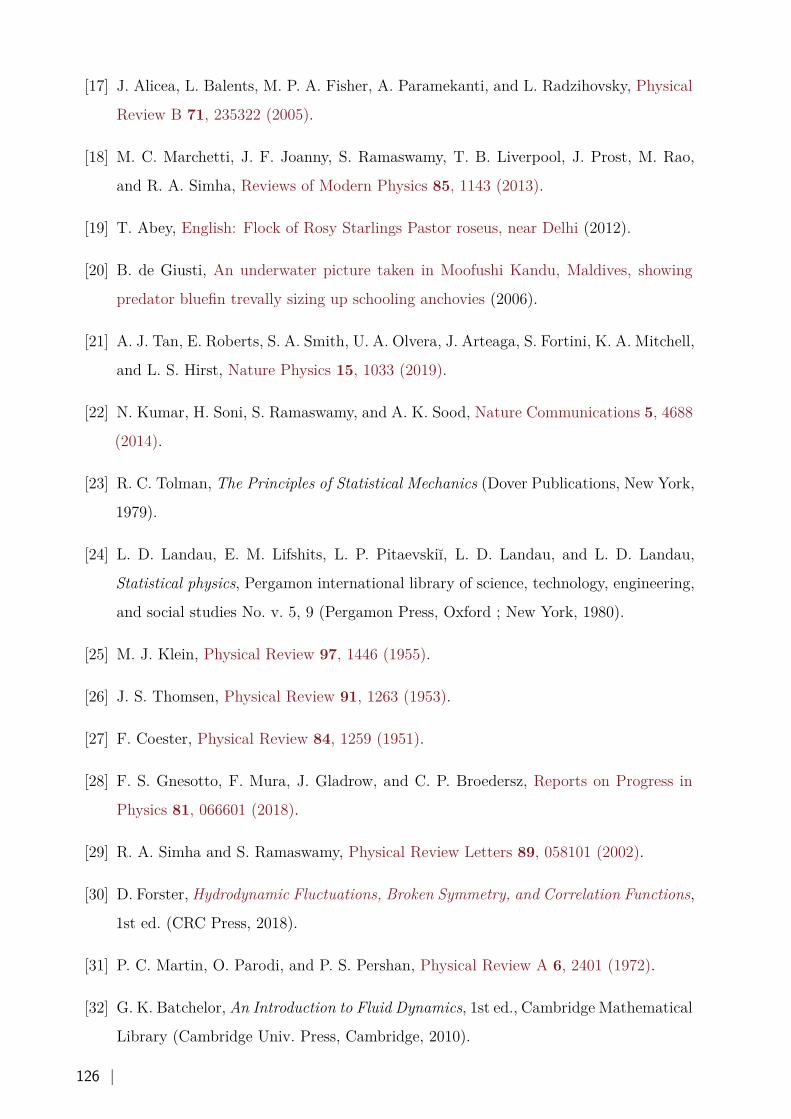
[17] J. Alicea, L. Balents, M. P. A. Fisher, A. Paramekanti, and L. Radzihovsky, Physical
Review B 71, 235322 (2005).
[18] M. C. Marchetti, J. F. Joanny, S. Ramaswamy, T. B. Liverpool, J. Prost, M. Rao,
and R. A. Simha, Reviews of Modern Physics 85, 1143 (2013).
[19] T. Abey, English: Flock of Rosy Starlings Pastor roseus, near Delhi (2012).
[20] B. de Giusti, An underwater picture taken in Moofushi Kandu, Maldives, showing
predator bluefin trevally sizing up schooling anchovies (2006).
[21] A. J. Tan, E. Roberts, S. A. Smith, U. A. Olvera, J. Arteaga, S. Fortini, K. A. Mitchell,
and L. S. Hirst, Nature Physics 15, 1033 (2019).
[22] N. Kumar, H. Soni, S. Ramaswamy, and A. K. Sood, Nature Communications 5, 4688
(2014).
[23] R. C. Tolman, The Principles of Statistical Mechanics (Dover Publications, New York,
1979).
[24] L. D. Landau, E. M. Lifshits, L. P. Pitaevskiĭ, L. D. Landau, and L. D. Landau,
Statistical physics, Pergamon international library of science, technology, engineering,
and social studies No. v. 5, 9 (Pergamon Press, Oxford ; New York, 1980).
[25] M. J. Klein, Physical Review 97, 1446 (1955).
[26] J. S. Thomsen, Physical Review 91, 1263 (1953).
[27] F. Coester, Physical Review 84, 1259 (1951).
[28] F. S. Gnesotto, F. Mura, J. Gladrow, and C. P. Broedersz, Reports on Progress in
Physics 81, 066601 (2018).
[29] R. A. Simha and S. Ramaswamy, Physical Review Letters 89, 058101 (2002).
[30] D. Forster, Hydrodynamic Fluctuations, Broken Symmetry, and Correlation Functions,
1st ed. (CRC Press, 2018).
[31] P. C. Martin, O. Parodi, and P. S. Pershan, Physical Review A 6, 2401 (1972).
[32] G. K. Batchelor, An Introduction to Fluid Dynamics, 1st ed., Cambridge Mathematical
Library (Cambridge Univ. Press, Cambridge, 2010).
126 |
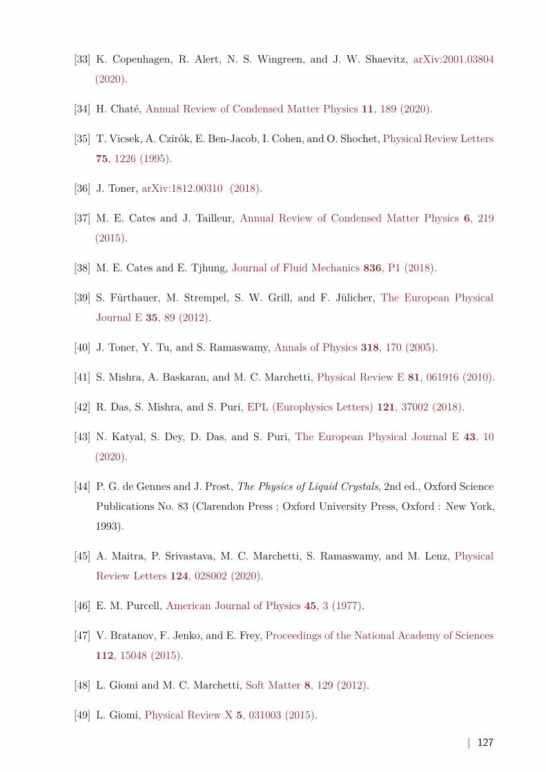
[33] K. Copenhagen, R. Alert, N. S. Wingreen, and J. W. Shaevitz, arXiv:2001.03804
(2020).
[34] H. Chaté, Annual Review of Condensed Matter Physics 11, 189 (2020).
[35] T. Vicsek, A. Czirók, E. Ben-Jacob, I. Cohen, and O. Shochet, Physical Review Letters
75, 1226 (1995).
[36] J. Toner, arXiv:1812.00310 (2018).
[37] M. E. Cates and J. Tailleur, Annual Review of Condensed Matter Physics 6, 219
(2015).
[38] M. E. Cates and E. Tjhung, Journal of Fluid Mechanics 836, P1 (2018).
[39] S. Fürthauer, M. Strempel, S. W. Grill, and F. Jülicher, The European Physical
Journal E 35, 89 (2012).
[40] J. Toner, Y. Tu, and S. Ramaswamy, Annals of Physics 318, 170 (2005).
[41] S. Mishra, A. Baskaran, and M. C. Marchetti, Physical Review E 81, 061916 (2010).
[42] R. Das, S. Mishra, and S. Puri, EPL (Europhysics Letters) 121, 37002 (2018).
[43] N. Katyal, S. Dey, D. Das, and S. Puri, The European Physical Journal E 43, 10
(2020).
[44] P. G. de Gennes and J. Prost, The Physics of Liquid Crystals, 2nd ed., Oxford Science
Publications No. 83 (Clarendon Press ; Oxford University Press, Oxford : New York,
1993).
[45] A. Maitra, P. Srivastava, M. C. Marchetti, S. Ramaswamy, and M. Lenz, Physical
Review Letters 124, 028002 (2020).
[46] E. M. Purcell, American Journal of Physics 45, 3 (1977).
[47] V. Bratanov, F. Jenko, and E. Frey, Proceedings of the National Academy of Sciences
112, 15048 (2015).
[48] L. Giomi and M. C. Marchetti, Soft Matter 8, 129 (2012).
[49] L. Giomi, Physical Review X 5, 031003 (2015).
| 127
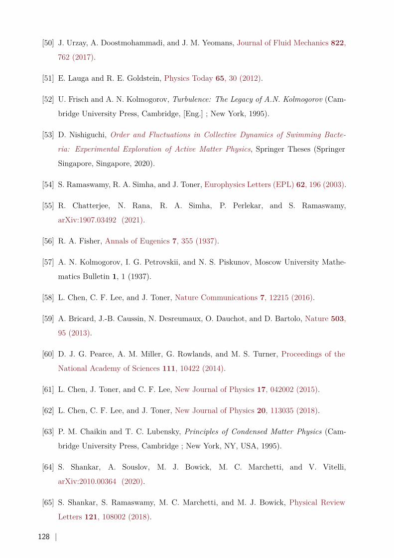
[50] J. Urzay, A. Doostmohammadi, and J. M. Yeomans, Journal of Fluid Mechanics 822,
762 (2017).
[51] E. Lauga and R. E. Goldstein, Physics Today 65, 30 (2012).
[52] U. Frisch and A. N. Kolmogorov, Turbulence: The Legacy of A.N. Kolmogorov (Cam-
bridge University Press, Cambridge, [Eng.] ; New York, 1995).
[53] D. Nishiguchi, Order and Fluctuations in Collective Dynamics of Swimming Bacte-
ria: Experimental Exploration of Active Matter Physics, Springer Theses (Springer
Singapore, Singapore, 2020).
[54] S. Ramaswamy, R. A. Simha, and J. Toner, Europhysics Letters (EPL) 62, 196 (2003).
[55] R. Chatterjee, N. Rana, R. A. Simha, P. Perlekar, and S. Ramaswamy,
arXiv:1907.03492 (2021).
[56] R. A. Fisher, Annals of Eugenics 7, 355 (1937).
[57] A. N. Kolmogorov, I. G. Petrovskii, and N. S. Piskunov, Moscow University Mathe-
matics Bulletin 1, 1 (1937).
[58] L. Chen, C. F. Lee, and J. Toner, Nature Communications 7, 12215 (2016).
[59] A. Bricard, J.-B. Caussin, N. Desreumaux, O. Dauchot, and D. Bartolo, Nature 503,
95 (2013).
[60] D. J. G. Pearce, A. M. Miller, G. Rowlands, and M. S. Turner, Proceedings of the
National Academy of Sciences 111, 10422 (2014).
[61] L. Chen, J. Toner, and C. F. Lee, New Journal of Physics 17, 042002 (2015).
[62] L. Chen, C. F. Lee, and J. Toner, New Journal of Physics 20, 113035 (2018).
[63] P. M. Chaikin and T. C. Lubensky, Principles of Condensed Matter Physics (Cam-
bridge University Press, Cambridge ; New York, NY, USA, 1995).
[64] S. Shankar, A. Souslov, M. J. Bowick, M. C. Marchetti, and V. Vitelli,
arXiv:2010.00364 (2020).
[65] S. Shankar, S. Ramaswamy, M. C. Marchetti, and M. J. Bowick, Physical Review
Letters 121, 108002 (2018).
128 |
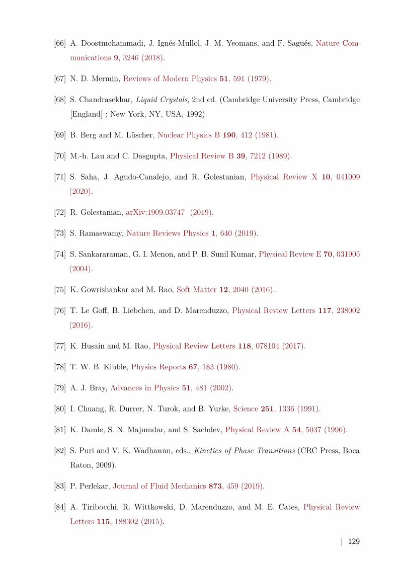
[66] A. Doostmohammadi, J. Ignés-Mullol, J. M. Yeomans, and F. Sagués, Nature Com-
munications 9, 3246 (2018).
[67] N. D. Mermin, Reviews of Modern Physics 51, 591 (1979).
[68] S. Chandrasekhar, Liquid Crystals, 2nd ed. (Cambridge University Press, Cambridge
[England] ; New York, NY, USA, 1992).
[69] B. Berg and M. Lüscher, Nuclear Physics B 190, 412 (1981).
[70] M.-h. Lau and C. Dasgupta, Physical Review B 39, 7212 (1989).
[71] S. Saha, J. Agudo-Canalejo, and R. Golestanian, Physical Review X 10, 041009
(2020).
[72] R. Golestanian, arXiv:1909.03747 (2019).
[73] S. Ramaswamy, Nature Reviews Physics 1, 640 (2019).
[74] S. Sankararaman, G. I. Menon, and P. B. Sunil Kumar, Physical Review E 70, 031905
(2004).
[75] K. Gowrishankar and M. Rao, Soft Matter 12, 2040 (2016).
[76] T. Le Goff, B. Liebchen, and D. Marenduzzo, Physical Review Letters 117, 238002
(2016).
[77] K. Husain and M. Rao, Physical Review Letters 118, 078104 (2017).
[78] T. W. B. Kibble, Physics Reports 67, 183 (1980).
[79] A. J. Bray, Advances in Physics 51, 481 (2002).
[80] I. Chuang, R. Durrer, N. Turok, and B. Yurke, Science 251, 1336 (1991).
[81] K. Damle, S. N. Majumdar, and S. Sachdev, Physical Review A 54, 5037 (1996).
[82] S. Puri and V. K. Wadhawan, eds., Kinetics of Phase Transitions (CRC Press, Boca
Raton, 2009).
[83] P. Perlekar, Journal of Fluid Mechanics 873, 459 (2019).
[84] A. Tiribocchi, R. Wittkowski, D. Marenduzzo, and M. E. Cates, Physical Review
Letters 115, 188302 (2015).
| 129
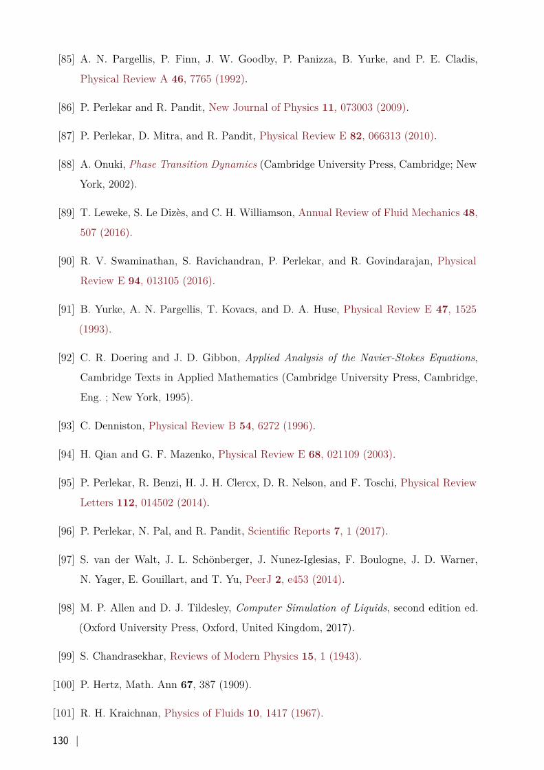
[85] A. N. Pargellis, P. Finn, J. W. Goodby, P. Panizza, B. Yurke, and P. E. Cladis,
Physical Review A 46, 7765 (1992).
[86] P. Perlekar and R. Pandit, New Journal of Physics 11, 073003 (2009).
[87] P. Perlekar, D. Mitra, and R. Pandit, Physical Review E 82, 066313 (2010).
[88] A. Onuki, Phase Transition Dynamics (Cambridge University Press, Cambridge; New
York, 2002).
[89] T. Leweke, S. Le Dizès, and C. H. Williamson, Annual Review of Fluid Mechanics 48,
507 (2016).
[90] R. V. Swaminathan, S. Ravichandran, P. Perlekar, and R. Govindarajan, Physical
Review E 94, 013105 (2016).
[91] B. Yurke, A. N. Pargellis, T. Kovacs, and D. A. Huse, Physical Review E 47, 1525
(1993).
[92] C. R. Doering and J. D. Gibbon, Applied Analysis of the Navier-Stokes Equations,
Cambridge Texts in Applied Mathematics (Cambridge University Press, Cambridge,
Eng. ; New York, 1995).
[93] C. Denniston, Physical Review B 54, 6272 (1996).
[94] H. Qian and G. F. Mazenko, Physical Review E 68, 021109 (2003).
[95] P. Perlekar, R. Benzi, H. J. H. Clercx, D. R. Nelson, and F. Toschi, Physical Review
Letters 112, 014502 (2014).
[96] P. Perlekar, N. Pal, and R. Pandit, Scientific Reports 7, 1 (2017).
[97] S. van der Walt, J. L. Schönberger, J. Nunez-Iglesias, F. Boulogne, J. D. Warner,
N. Yager, E. Gouillart, and T. Yu, PeerJ 2, e453 (2014).
[98] M. P. Allen and D. J. Tildesley, Computer Simulation of Liquids, second edition ed.
(Oxford University Press, Oxford, United Kingdom, 2017).
[99] S. Chandrasekhar, Reviews of Modern Physics 15, 1 (1943).
[100] P. Hertz, Math. Ann 67, 387 (1909).
[101] R. H. Kraichnan, Physics of Fluids 10, 1417 (1967).
130 |
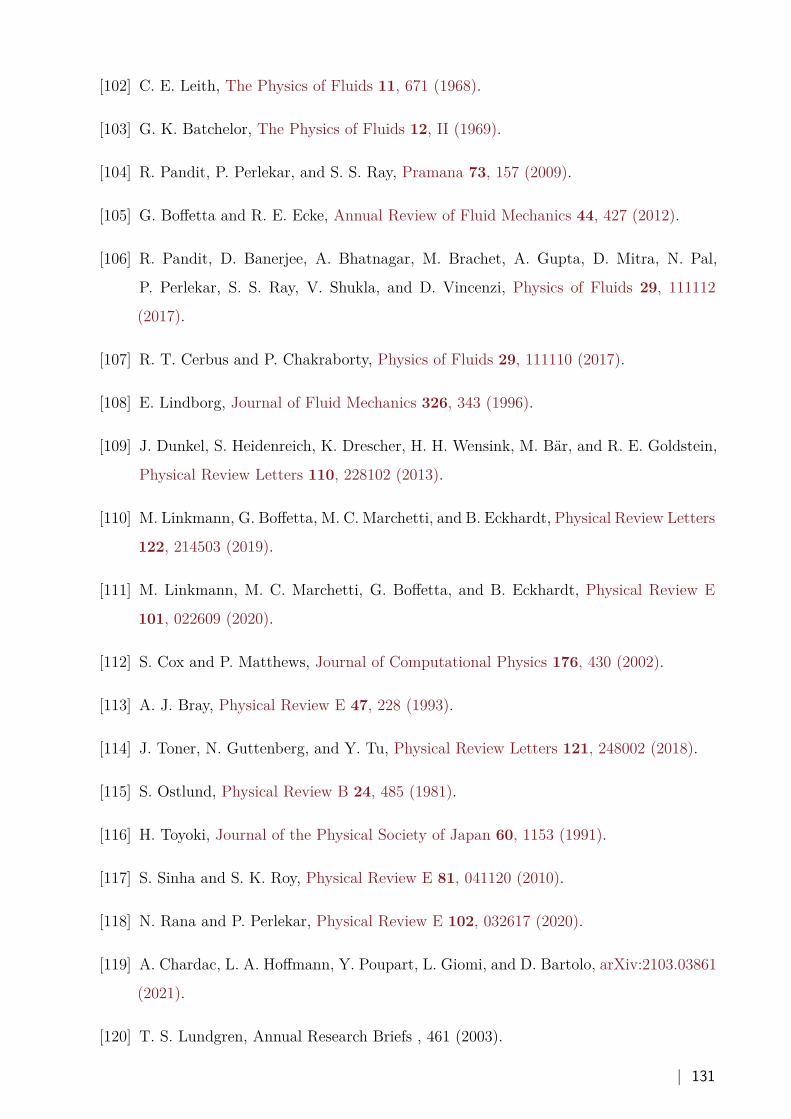
[102] C. E. Leith, The Physics of Fluids 11, 671 (1968).
[103] G. K. Batchelor, The Physics of Fluids 12, II (1969).
[104] R. Pandit, P. Perlekar, and S. S. Ray, Pramana 73, 157 (2009).
[105] G. Boffetta and R. E. Ecke, Annual Review of Fluid Mechanics 44, 427 (2012).
[106] R. Pandit, D. Banerjee, A. Bhatnagar, M. Brachet, A. Gupta, D. Mitra, N. Pal,
P. Perlekar, S. S. Ray, V. Shukla, and D. Vincenzi, Physics of Fluids 29, 111112
(2017).
[107] R. T. Cerbus and P. Chakraborty, Physics of Fluids 29, 111110 (2017).
[108] E. Lindborg, Journal of Fluid Mechanics 326, 343 (1996).
[109] J. Dunkel, S. Heidenreich, K. Drescher, H. H. Wensink, M. Bär, and R. E. Goldstein,
Physical Review Letters 110, 228102 (2013).
[110] M. Linkmann, G. Boffetta, M. C. Marchetti, and B. Eckhardt, Physical Review Letters
122, 214503 (2019).
[111] M. Linkmann, M. C. Marchetti, G. Boffetta, and B. Eckhardt, Physical Review E
101, 022609 (2020).
[112] S. Cox and P. Matthews, Journal of Computational Physics 176, 430 (2002).
[113] A. J. Bray, Physical Review E 47, 228 (1993).
[114] J. Toner, N. Guttenberg, and Y. Tu, Physical Review Letters 121, 248002 (2018).
[115] S. Ostlund, Physical Review B 24, 485 (1981).
[116] H. Toyoki, Journal of the Physical Society of Japan 60, 1153 (1991).
[117] S. Sinha and S. K. Roy, Physical Review E 81, 041120 (2010).
[118] N. Rana and P. Perlekar, Physical Review E 102, 032617 (2020).
[119] A. Chardac, L. A. Hoffmann, Y. Poupart, L. Giomi, and D. Bartolo, arXiv:2103.03861
(2021).
[120] T. S. Lundgren, Annual Research Briefs , 461 (2003).
| 131
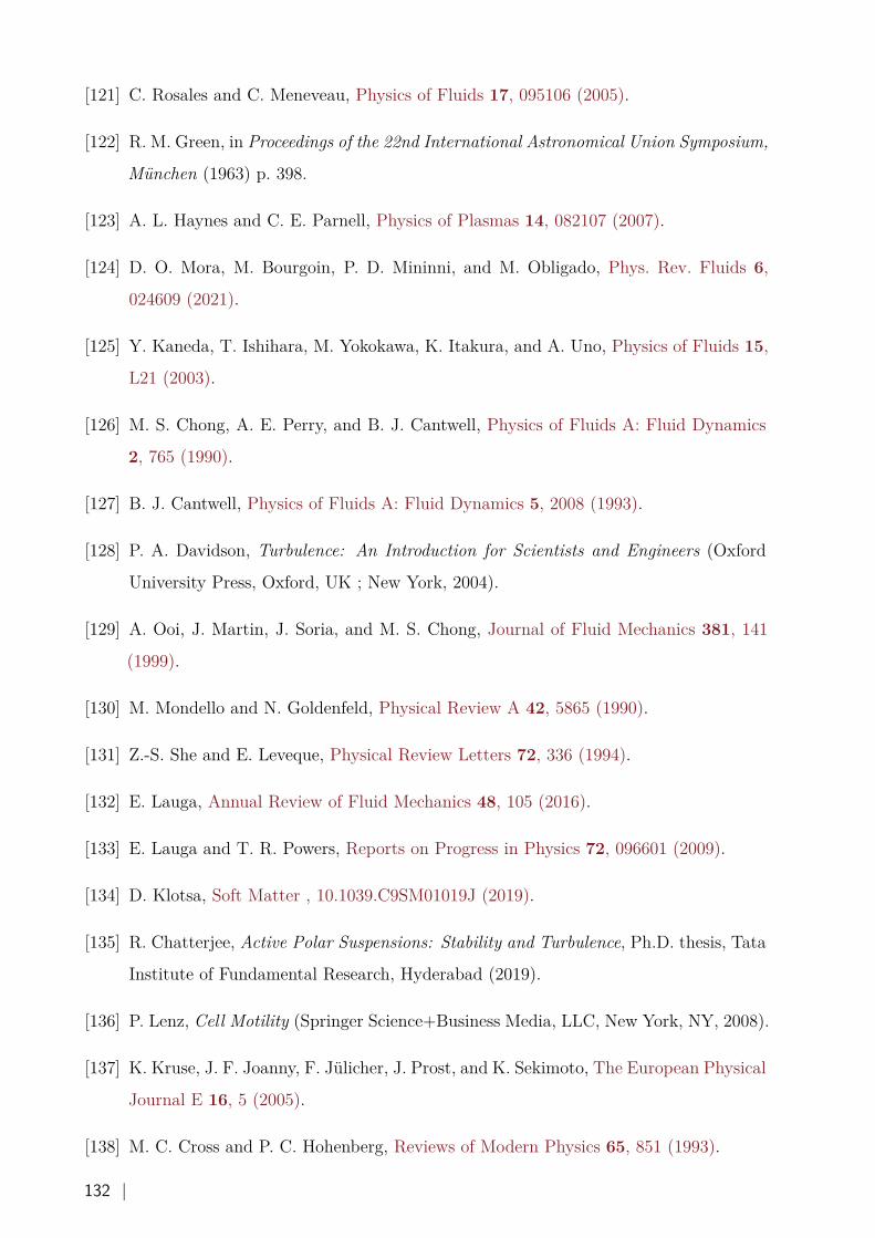
[121] C. Rosales and C. Meneveau, Physics of Fluids 17, 095106 (2005).
[122] R. M. Green, in Proceedings of the 22nd International Astronomical Union Symposium,
München (1963) p. 398.
[123] A. L. Haynes and C. E. Parnell, Physics of Plasmas 14, 082107 (2007).
[124] D. O. Mora, M. Bourgoin, P. D. Mininni, and M. Obligado, Phys. Rev. Fluids 6,
024609 (2021).
[125] Y. Kaneda, T. Ishihara, M. Yokokawa, K. Itakura, and A. Uno, Physics of Fluids 15,
L21 (2003).
[126] M. S. Chong, A. E. Perry, and B. J. Cantwell, Physics of Fluids A: Fluid Dynamics
2, 765 (1990).
[127] B. J. Cantwell, Physics of Fluids A: Fluid Dynamics 5, 2008 (1993).
[128] P. A. Davidson, Turbulence: An Introduction for Scientists and Engineers (Oxford
University Press, Oxford, UK ; New York, 2004).
[129] A. Ooi, J. Martin, J. Soria, and M. S. Chong, Journal of Fluid Mechanics 381, 141
(1999).
[130] M. Mondello and N. Goldenfeld, Physical Review A 42, 5865 (1990).
[131] Z.-S. She and E. Leveque, Physical Review Letters 72, 336 (1994).
[132] E. Lauga, Annual Review of Fluid Mechanics 48, 105 (2016).
[133] E. Lauga and T. R. Powers, Reports on Progress in Physics 72, 096601 (2009).
[134] D. Klotsa, Soft Matter , 10.1039.C9SM01019J (2019).
[135] R. Chatterjee, Active Polar Suspensions: Stability and Turbulence, Ph.D. thesis, Tata
Institute of Fundamental Research, Hyderabad (2019).
[136] P. Lenz, Cell Motility (Springer Science+Business Media, LLC, New York, NY, 2008).
[137] K. Kruse, J. F. Joanny, F. Jülicher, J. Prost, and K. Sekimoto, The European Physical
Journal E 16, 5 (2005).
[138] M. C. Cross and P. C. Hohenberg, Reviews of Modern Physics 65, 851 (1993).
132 |
[139] S. Kondo and T. Miura, Science 329, 1616 (2010).
[140] J.-i. Wakita, K. Komatsu, A. Nakahara, T. Matsuyama, and M. Matsushita, Journal
of the Physical Society of Japan 63, 1205 (1994).
[141] D. Woodward, R. Tyson, M. Myerscough, J. Murray, E. Budrene, and H. Berg, Bio-
physical Journal 68, 2181 (1995).
[142] J. A. Shapiro, BioEssays 17, 597 (1995).
[143] E. Ben-Jacob, I. Cohen, and D. L. Gutnick, Annual Review of Microbiology 52, 779
(1998).
[144] N. Verstraeten, K. Braeken, B. Debkumari, M. Fauvart, J. Fransaer, J. Vermant, and
J. Michiels, Trends in Microbiology 16, 496 (2008).
[145] P. Deng, L. de Vargas Roditi, D. van Ditmarsch, and J. B. Xavier, New Journal of
Physics 16, 015006 (2014).
[146] A. Mitchell and J. Wimpenny, Journal of Applied Microbiology 83, 76 (1997).
[147] R. M. Harshey, Annual Review of Microbiology 57, 249 (2003).
[148] H. Shimada, T. Ikeda, J.-i. Wakita, H. Itoh, S. Kurosu, F. Hiramatsu, M. Nakatsuchi,
Y. Yamazaki, T. Matsuyama, and M. Matsushita, Journal of the Physical Society of
Japan 73, 1082 (2004).
[149] C. Kaito and K. Sekimizu, Journal of Bacteriology 189, 2553 (2007).
[150] M. Fauvart, P. Phillips, D. Bachaspatimayum, N. Verstraeten, J. Fransaer, J. Michiels,
and J. Vermant, Soft Matter 8, 70 (2012).
[151] P. Kumar and A. Libchaber, Biophysical Journal 105, 783 (2013).
[152] M. Deforet, D. van Ditmarsch, C. Carmona-Fontaine, and J. B. Xavier, Soft Matter
10, 2405 (2014).
[153] C. Giverso, M. Verani, and P. Ciarletta, Journal of The Royal Society Interface 12,
20141290 (2015).
[154] Y. Wu, Quantitative Biology 3, 199 (2015).
| 133
[155] M. Matsushita, J. Wakita, H. Itoh, I. Ràfols, T. Matsuyama, H. Sakaguchi, and
M. Mimura, Physica A: Statistical Mechanics and its Applications 249, 517 (1998).
[156] E. Ben-Jacob, I. Cohen, and H. Levine, Advances in Physics 49, 395 (2000).
[157] T. Sams, K. Sneppen, M. H. Jensen, C. Ellegaard, B. E. Christensen, and U. Thrane,
Physical Review Letters 79, 313 (1997).
[158] E. Ben-Jacob, O. Schochet, A. Tenenbaum, I. Cohen, A. Czirók, and T. Vicsek, Nature
368, 46 (1994).
[159] K. Kawasaki, A. Mochizuki, M. Matsushita, T. Umeda, and N. Shigesada, Journal of
Theoretical Biology 188, 177 (1997).
[160] I. Golding, Y. Kozlovsky, I. Cohen, and E. Ben-Jacob, Physica A: Statistical Mechan-
ics and its Applications 260, 510 (1998).
[161] P. Ghosh, E. Ben-Jacob, and H. Levine, Physical Biology 10, 066006 (2013).
[162] P. Patra, K. Kissoon, I. Cornejo, H. B. Kaplan, and O. A. Igoshin, PLOS Computa-
tional Biology 12, e1005010 (2016).
[163] D. Schwarcz, H. Levine, E. Ben-Jacob, and G. Ariel, Physica D: Nonlinear Phenomena
318-319, 91 (2016).
[164] K. S. Korolev, J. B. Xavier, D. R. Nelson, and K. R. Foster, The American Naturalist
178, 538 (2011).
[165] F. D. C. Farrell, O. Hallatschek, D. Marenduzzo, and B. Waclaw, Physical Review
Letters 111, 168101 (2013).
[166] P. Ghosh, J. Mondal, E. Ben-Jacob, and H. Levine, Proceedings of the National
Academy of Sciences 112, E2166 (2015).
[167] C. R. Doering, C. Mueller, and P. Smereka, Physica A: Statistical Mechanics and its
Applications Stochastic Systems: From Randomness to Complexity, 325, 243 (2003).
[168] P. Perlekar, R. Benzi, D. R. Nelson, and F. Toschi, Journal of Physics: Conference
Series 318, 092025 (2011).
[169] R. Benzi, M. H. Jensen, D. R. Nelson, P. Perlekar, S. Pigolotti, and F. Toschi, The
European Physical Journal Special Topics 204, 57 (2012).
134 |
[170] S. Pigolotti, R. Benzi, P. Perlekar, M. H. Jensen, F. Toschi, and D. R. Nelson, Theo-
retical Population Biology 84, 72 (2013).
[171] A. M. Lacasta, I. R. Cantalapiedra, C. E. Auguet, A. Peñaranda, and L. Ramírez-
Piscina, Physical Review E 59, 7036 (1999).
[172] E. Ben-Jacob, I. Cohen, A. Czirók, T. Vicsek, and D. L. Gutnick, Physica A: Statis-
tical Mechanics and its Applications 238, 181 (1997).
[173] D. A. Kessler and H. Levine, Nature 394, 556 (1998).
[174] S. Nesic, R. Cuerno, and E. Moro, Physical Review Letters 113, 180602 (2014).
[175] I. Dornic, H. Chaté, and M. A. Muñoz, Physical Review Letters 94, 100601 (2005).
[176] O. Hallatschek and K. S. Korolev, Physical Review Letters 103, 108103 (2009).
[177] E. Brunet and B. Derrida, Physical Review E 56, 2597 (1997).
[178] S. Pigolotti and R. Benzi, Physical Review Letters 112, 188102 (2014).
[179] L. Pechenik and H. Levine, Physical Review E 59, 3893 (1999).
[180] A. Jeffrey and H.-H. Dai, Handbook of Mathematical Formulas and Integrals, 4th ed.
(Academic Press/Elsevier, Burlington, MA, 2008).
[181] L. Devroye, Non-Uniform Random Variate Generation (Springer, New York, 1986).
[182] M. Galassi, ed., GNU Scientific Library: Reference Manual, 3rd ed., A GNU Manual
(Network Theory, s.l., 2009).
[183] J. A. Bonachela, C. D. Nadell, J. B. Xavier, and S. A. Levin, Journal of Statistical
Physics 144, 303 (2011).
[184] A.-L. Barabási, H. E. Stanley, and Cambridge University Press, Fractal concepts in
surface growth (Cambridge University Press, New York, N.Y., 1995).
[185] N. Rana, P. Ghosh, and P. Perlekar, Physical Review E 96, 052403 (2017).
[186] M. Asally, M. Kittisopikul, P. Rue, Y. Du, Z. Hu, T. Cagatay, A. B. Robinson, H. Lu,
J. Garcia-Ojalvo, and G. M. Suel, Proceedings of the National Academy of Sciences
109, 18891 (2012).
| 135
[187] A. N. Kolmogorov, Proceedings: Mathematical and Physical Sciences 434, 9 (1991).
[188] A. N. Kolmogorov, Proceedings: Mathematical and Physical Sciences 434, 15 (1991).
[189] J. von Neumann, in Collected Works (1949-1963), Vol. 6 (Pergamon Press, 1963) pp.
437–472.
[190] S. A. Orszag, The Physics of Fluids 12, II (1969).
[191] S. A. Orszag, Journal of Fluid Mechanics 49, 75 (1971).
[192] S. A. Orszag, Journal of the Atmospheric Sciences 28, 1074 (1971).
[193] S. A. Orszag and G. S. Patterson, Statistical Models and Turbulence , 127 (1972).
[194] S. A. Orszag, Journal of Computational Physics 37, 70 (1980).
[195] J. W. Cooley and J. W. Tukey, Mathematics of Computation 19, 297 (1965).
[196] K. P. Iyer, K. R. Sreenivasan, and P. K. Yeung, Physical Review X 9, 041006 (2019).
[197] A. Nukada, K. Sato, and S. Matsuoka, in SC ’12: Proceedings of the International
Conference on High Performance Computing, Networking, Storage and Analysis (2012)
pp. 1–10.
[198] K. Czechowski, C. Battaglino, C. McClanahan, K. Iyer, P.-K. Yeung, and R. Vuduc,
in Proceedings of the 26th ACM International Conference on Supercomputing - ICS
’12 (ACM Press, San Servolo Island, Venice, Italy, 2012) p. 205.
[199] A. Gholami, J. Hill, D. Malhotra, and G. Biros, arXiv:1506.07933 (2016).
[200] G. K. Batchelor, The Theory of Homogeneous Turbulence, Cambridge Science Classics
(Cambridge University Press, Cambridge ; New York, 1982).
[201] S. B. Pope, Turbulent Flows (Cambridge University Press, Cambridge ; New York,
2000).
[202] C. Canuto, M. Y. Hussaini, A. Quarteroni, and T. A. Zang, Spectral Methods in Fluid
Dynamics (Springer Berlin Heidelberg, Berlin, Heidelberg, 1988).
[203] R. S. Rogallo, Numerical Experiments in Homogeneous Turbulence, Tech. Rep. (NASA,
1981).
[204] A. Shapiro, Monthly Weather Review 121, 2420 (1993).
136 |