ARTICLEdoi:10.1038/nature11229
Deep carbon export from a SouthernOcean iron-fertilized diatom bloomVictor Smetacek1,2*, Christine Klaas1*, Volker H. Strass1, Philipp Assmy1,3, Marina Montresor4, Boris Cisewski1,5, Nicolas Savoye6,7,Adrian Webb8, Francesco d’Ovidio9, Jesus M. Arrieta10,11, Ulrich Bathmann1,12, Richard Bellerby13,14, Gry Mine Berg15,Peter Croot16,17, Santiago Gonzalez10, Joachim Henjes1,18, Gerhard J. Herndl10,19, Linn J. Hoffmann16, Harry Leach20, Martin Losch1,Matthew M. Mills15, Craig Neill13,21, Ilka Peeken1,22, Rudiger Rottgers23, Oliver Sachs1,24, Eberhard Sauter1, Maike M. Schmidt25,Jill Schwarz1,26, Anja Terbruggen1 & Dieter Wolf-Gladrow1
Fertilization of the ocean by adding iron compounds has induced diatom-dominated phytoplankton bloomsaccompanied by considerable carbon dioxide drawdown in the ocean surface layer. However, because the fate ofbloom biomass could not be adequately resolved in these experiments, the timescales of carbon sequestration fromthe atmosphere are uncertain. Here we report the results of a five-week experiment carried out in the closed core of avertically coherent, mesoscale eddy of the Antarctic Circumpolar Current, during which we tracked sinking particlesfrom the surface to the deep-sea floor. A large diatom bloom peaked in the fourth week after fertilization. This wasfollowed by mass mortality of several diatom species that formed rapidly sinking, mucilaginous aggregates of entangledcells and chains. Taken together, multiple lines of evidence—although each with important uncertainties—lead us toconclude that at least half the bloom biomass sank far below a depth of 1,000 metres and that a substantial portion islikely to have reached the sea floor. Thus, iron-fertilized diatom blooms may sequester carbon for timescales of centuriesin ocean bottom water and for longer in the sediments.
The Southern Ocean is regarded as a likely source and sink of atmo-spheric CO2 over glacial–interglacial climate cycles, but the relativeimportance of physical and biological mechanisms driving CO2
exchange are under debate1,2. The iron hypothesis3, which is basedon iron limitation of phytoplankton growth in extensive, nutrient-rich areas of today’s oceans, is that the greater supply of iron-bearingdust to these regions during the dry glacials stimulated phytoplanktonblooms that, by sinking from the surface to the deep ocean, sequesteredclimatically relevant amounts of carbon from exchange with the atmo-sphere. Twelve ocean iron fertilization (OIF) experiments carried outto test this hypothesis have provided unambiguous support for the firstcondition: that iron addition generates phytoplankton blooms inregions with high nutrient but low chlorophyll concentrations includ-ing the Southern Ocean4,5. The findings are consistent with satelliteobservations of natural phytoplankton blooms in these regions stimu-lated by dust input from continental6 and volcanic7 sources.
The timescales on which CO2 taken up by phytoplankton issequestered from the atmosphere depend on the depths at whichorganic matter sinking out of the surface layer is subsequentlyremineralized back to CO2 by microbes and zooplankton. In the
Southern Ocean, the portion of CO2 retained within the 200-m-deepwinter mixed layer would be in contact with the atmosphere withinmonths, but carbon sinking to successively deeper layers, and finallythe sediments, will be sequestered for decades to centuries or longer.Previous OIF experiments have not adequately demonstrated the fateand depth of sinking of bloom biomass5, so it is uncertain whethermass, deep-sinking events comparable to those observed in theaftermath of natural blooms8 also ensue from OIF blooms.Furthermore, palaeo-oceanographic proxies from the underlyingsediments are ambiguous regarding productivity of the glacialSouthern Ocean1,2,9,10. Hence, the second condition of the iron hypo-thesis, that OIF-generated biomass sinks to greater depths, has yet tobe confirmed. The issue is currently receiving broad attention becauseOIF is one of the techniques listed in the geoengineering portfolio tomitigate the effects of climate change11.
Monitoring the sinking flux from an experimental bloom requiresvertical coherence between surface and deeper layers, a conditionfulfilled by the closed cores of mesoscale eddies formed by meanderingfrontal jets of the Antarctic Circumpolar Current, which are prom-inent in satellite altimeter images as sea surface height anomalies12. An
*These authors contributed equally to this work.
1Alfred Wegener Institute for Polar and Marine Research, Am Handelshafen 12, 27570 Bremerhaven, Germany. 2National Institute of Oceanography, Dona Paula, Goa 403 004, India. 3Norwegian PolarInstitute, Fram Centre, Hjalmar Johansens Gate 14, 9296 Tromsø, Norway. 4Ecology and Evolution of Plankton, Stazione Zoologica Anton Dohrn, Villa Comunale, 80121-Napoli, Italy. 5Johann Heinrich vonThunen Institute, Institute of Sea Fisheries, Palmaille 9, 22767 Hamburg, Germany. 6Department of Analytical and Environmental Chemistry, Vrije Universiteit Brussel, Pleinlaan 2, 1050 Brussels, Belgium.7Univ. Bordeaux/CNRS, EPOC, UMR 5805, Station Marine d’Arcachon, 2 rue du Professeur Jolyet, F-33120 Arcachon, France. 8Oceanography Department, University of Cape Town, Private Bag X3,Rondebosch, 7701 Cape Town, South Africa. 9LOCEAN-IPSL, CNRS/UPMC/IRD/MNHN, 4 Place Jussieu, 75252 Paris Cedex 5, France. 10Department of Biological Oceanography, Royal NetherlandsInstitute for Sea Research, PO Box 59, 1790 AB Den Burg, The Netherlands. 11Department of Global Change Research, Instituto Mediterraneo de Estudios Avanzados, CSIC-UIB, Miquel Marques 21, 07190Esporles, Mallorca, Spain. 12Leibniz Institute for Baltic Sea Research Warnemunde, Seestraße 15, 18119 Rostock, Germany. 13Bjerknes Centre for Climate Research, University of Bergen, Allegaten 55,N-5007 Bergen, Norway. 14Norwegian Institute for Water Research, Thormøhlensgate 53 D, 5006 Bergen, Norway. 15Department of Environmental Earth System Science, Stanford University, Stanford,California 94305, USA. 16Helmholtz Centre for Ocean Research Kiel, Dusternbrooker Weg 20, 24105 Kiel, Germany. 17Earth and Ocean Sciences, School of Natural Sciences, National University of Ireland,Galway, Quadrangle Building, University Road, Galway, Ireland. 18Phytolutions GmbH, Campus Ring 1, 28759 Bremen, Germany. 19Department of Marine Biology, University of Vienna, Althanstrasse 14,1090 Vienna, Austria. 20School of Environmental Sciences, University of Liverpool, Room 209 Nicholson Building, 4 Brownlow Street, Liverpool L69 3GP, UK. 21Wealth from Oceans Flagship,Commonwealth Scientific and Industrial Research Organisation, Castray Esplanade, Hobart, Tasmania 7000, Australia. 22MARUM – Center for Marine Environmental Sciences, University of Bremen,Leobener Strasse, D-28359 Bremen, Germany. 23Institute for Coastal Research, Helmholtz-Zentrum Geesthacht, Center for Materials and Coastal Research, Max-Planck-Strasse 1, 21502 Geesthacht,Germany. 24Eberhard & Partner AG, General Guisan Strasse 2, 5000 Arau, Switzerland. 25Centre for Biomolecular Interactions Bremen, FB 2, University of Bremen, Postfach 33 04 40, 28359 Bremen,Germany. 26School of Marine Science & Engineering, Plymouth University, Drake Circus, Plymouth PL4 8AA, UK.
1 9 J U L Y 2 0 1 2 | V O L 4 8 7 | N A T U R E | 3 1 3
Macmillan Publishers Limited. All rights reserved©2012

added advantage offered by closed eddy cores is that processes occur-ring in the fertilized patch can be compared with natural processes inadjoining unfertilized waters of the same provenance.
The eddy and experimentThe European Iron Fertilization Experiment (EIFEX) was carried outfrom 11 February 2004 to 20 March 2004 during RV Polarstern cruiseANT XXI/3, in the clockwise-rotating core of an eddy formed by ameander of the Antarctic polar front (Fig. 1 and SupplementaryInformation). The eddy was mapped over a period of seven daysshortly after fertilization of the patch with a grid of 80 stations along
eight north–south transects 9 km apart. The rotating patch wasencountered on two of the grid transects. Measurements of currentspeed and direction with the vessel-mounted acoustic Dopplercurrent profiler and images of sea surface height anomalies revealeda closed, 60-km-diameter core clearly demarcated from the surround-ing meander of the Antarctic polar front in all measured physical,chemical and biological properties (Fig. 1a, b and SupplementaryInformation).
Estimates of geostrophic shear and transports derived from tem-perature and salinity profiles (Supplementary Figs 1 and 2) indicate acoherent surface-to-bottom eddy circulation that was almost closed
-18
-18
-16
-16
-16-16
-16
-14-14
-14
-14
-14
-14
-14
-12
-12
-12
-12
-12-12
-12
-12
-12
-10 -10
-10
-10
-10
-10-10
-10
-10
-10
-8
-8-8
-8
-8
-8
-8-8
-8
-8
-8
-8
-6
-6
-6
-6
-6
-6
-6
-6
-6
-6
-6
-6
-6
-6
-4
-4-4
-4
-4
-4-4
-4
-4
-4
-4
-4
-2
-2
-2-2
-2
-2
-2-2
-2
-2
-2
-2
0
0
0
0
00
0
0
0
0
0
0
00
0
0
2
2 22
2
2
4
4 44
4
6
66
6
8
8
8
10
10
30′15′2° E45′
49° S
50′
10′
20′
30′
40′
30′1–3/3/2004
30′15′2° E45′
49° S
50′
10′
20′
30′
40′
21.510.5
30′
2.5
23–24/2/2004
Chl (μg l–1)
Chl (μg l–1)
g h i48° S
50° S
52° S
48° S
50° S
52° S2–12 February 04 26 Feb–11 March 04 13–20 March 04
SSHA (cm)^ (1,000 m2 s–1)
a b
20′
49° S
40′
50° S30′
20′
40′
30′ 30′2° E 3° E
120
18/2/2004
6–6–18 –12120 6–6–18 –12
c
d e f
50 cm s–1
1° E 30′30′ 30′2° E 3° E1° E
21.510.5 2.5
30′15′2° E45′30′
0.450.35 0.55
1–3/3/2004
Fv/Fm fCO2 (μatm)
344 348 352 356 360
1–3/3/2004
49° S
50′
10′
20′
30′
40′
30′15′2° E45′30′
2° E0° E 4° E 2° E
Longitude
Latit
ude
0° E 4° E 2° E0° E 4° E
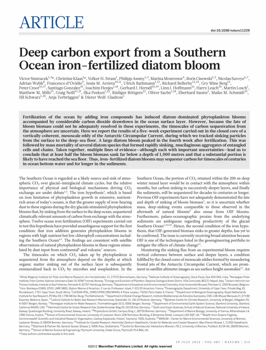
Figure 1 | Experimental eddy and the fertilized patch. a, The eddy coredepicted with the stream function (Y; contours and colour scale) derived fromcurrents measured using a vessel-mounted acoustic Doppler current profiler ata regular grid of stations between days 1 and 7. The black spiral is the ship’strack (a Lagrangian circle) around the buoy drifting southwestward duringfertilization. The white line is the superimposed track of the drifting buoyduring its first rotation from days 21 to 11 (same as in b and c). b, Altimeterimage of sea surface height anomaly (SSHA; contours and colour scale fromCCAR, http://argo.colorado.edu/,realtime/gsfc_global-real-time_ssh/.) Therectangle in a and b is enlarged in c–f. c, Area and location of the patch ondays 10 and 11 after fertilization, depicted on the basis of chlorophyll
measurements. The yellow area is the hot spot. d–f, Location and area of thepatch 17 days after fertilization, depicted in terms of photochemical efficiency(Fv/Fm; d), CO2 fugacity (fCO2; e) and chlorophyll concentration (f). The line isthe track of the drifting buoy during its second rotation (days 13–21). The redarea in f is the hot spot. g–i, Satellite-derived surface chlorophyll concentrationsof the EIFEX eddy before fertilization (g), during the bloom peak (h) and in itsdemise phase (i). The eddy core is encircled in white; the EIFEX bloom isevident in h and i (green colour is .1mg Chl l21). Note the natural bloom alongthe Antarctic polar front, which disappeared in this period. SeaWiFS images(g–i) courtesy of the NASA SeaWiFS Project and GeoEye.
RESEARCH ARTICLE
3 1 4 | N A T U R E | V O L 4 8 7 | 1 9 J U L Y 2 0 1 2
Macmillan Publishers Limited. All rights reserved©2012

and had little divergence. The vertical coherence of the eddy was alsorevealed by the congruent tracks of four neutrally buoyant floatspositioned at respective depths of 200, 300, 500 and 1,000 m(Supplementary Fig. 3). A post-cruise Lagrangian analysis based ondelayed-time altimetry13 showed that, for the entire duration of theexperiment, the compact core was only marginally eroded by lateralstirring, losing less than 10% of its content in total (SupplementaryInformation). This finding is consistent with diffusive heat budgetsderived from the observed warming of the eddy’s cold core14. Hence,the EIFEX eddy provided ideal conditions for monitoring the samewater column from the surface to the sea floor over time.
The site of the pre-fertilization control station was marked with adrifting buoy around which a circular patch of 167 km2 was fertilizedwith dissolved Fe(II) sulphate on 12–13 February (day 0) to yield aconcentration of 1.5 mmol Fe m23 in the 100-m-deep surface mixedlayer, which is greater than background values by a factor of aroundfive. A second fertilization on days 13 and 14 added an additional0.34 mmol Fe m23 to the 100-m-deep surface layer of the spreadingpatch. The patch was inadvertently placed off-centre but well withinthe closed eddy core and completed four rotations during the experi-ment. The area of the patch increased from 167 km2 on day 0 to447 km2 on day 11 and to 798 km2 on day 19 (Fig. 1c–f andSupplementary Information). ‘In-stations’ were taken in the least-diluted region of the patch: the ‘hot spot’ (Fig. 1c–f). ‘Out-stations’were taken within the eddy core well away from the patch but indifferent locations relative to it, and hence did not represent idealcontrols for quantifying processes within the patch.
Sampling frequency and depth coverage by discrete measurementsare illustrated by the vertical distributions of chlorophyll and silicateconcentrations (Fig. 2). Vertical profiles from in situ recording instru-ments indicated that the boundary of the mixed layer, defined by asharp dip in temperature, salinity, fluorescence and transmission, wasgenerally at a depth of 100 m (ref. 15; 97.6 6 20.6 m). The element andbiomass budgets presented here are based on inventories (in moles orgrams per square metre) derived from the trapezoidal integration ofsix to eight discrete measurements from the 100-m-deep surface layer.For comparison with other studies, the stocks (inventories) from thislayer are also presented where appropriate as depth-averaged concen-trations (in millimoles or milligrams per cubic metre).
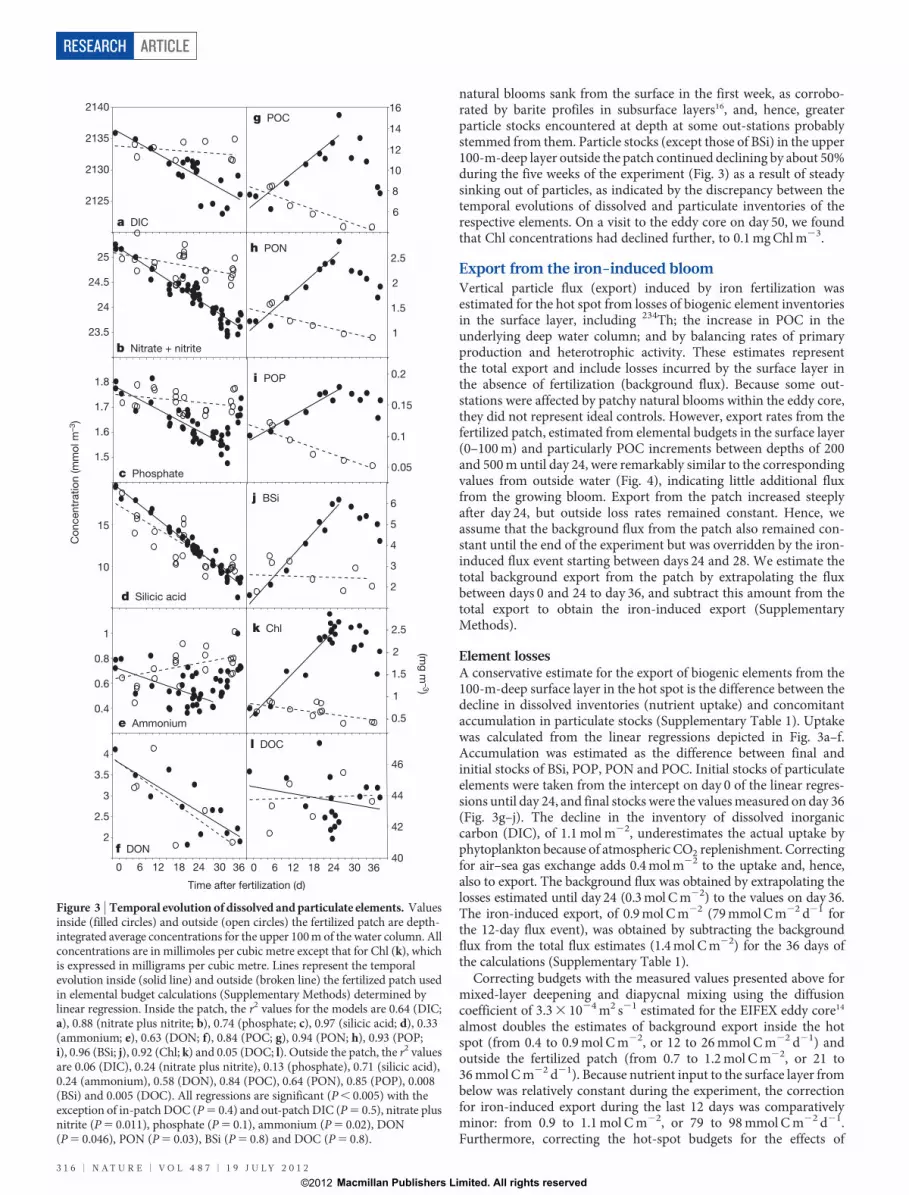
Processes inside and outside the patchEnhanced phytoplankton growth stimulated by iron fertilizationresulted in highly significant, linear increases in stocks of chlorophyll(Chl), particulate organic carbon (POC), nitrogen (PON), phosphate(POP) and biogenic silica (BSi) until day 24 (Figs 2a and 3). Thesestocks, depicted as depth-averaged concentrations in Fig. 3, declinedthereafter, although at different rates. However, inventories of thecorresponding dissolved nutrients, including dissolved organicnitrogen (DON), underwent a constant, linear decline until the endof the experiment, indicating that the respective uptake rates weremaintained throughout (Fig. 3). Detailed, visual, quantitative examina-tion of organisms and their remains across the entire size spectrum ofthe plankton revealed that population growth of many different speciesof large diatoms accounted for 97% of the Chl increase. The declineafter day 24 was caused by mass death and formation of rapidly sinkingaggregates by some diatom species, which was partly compensated bycontinued growth of other, heavily silicified species with high accu-mulation rates. The strikingly linear, instead of exponential, trends canbe attributed to the effects of patch dilution with surrounding waterbecause dilution rates (0.06–0.1 d21; Supplementary Information) andphytoplankton accumulation rates (0.03–0.11 d21) were similar.
The discrepancies in the budgets of particulate and dissolved poolsof the various elements in the surface layer can only be explained bythe sinking out of particles, as losses to dissolved organic pools canlargely be ruled out: stocks of dissolved organic carbon (DOC)remained stable (44 6 2 mmol C m23; Fig. 3l), those of DON halved(from 3.8 to 2.0 mmol N m23; Fig. 3f) and those of dissolved organicphosphate (not shown) were at the detection limit. The decline inDON was barely reflected in DOC because it was apparently asso-ciated with a relatively small, labile fraction with much lower C/Nratios than that of the large refractory DOC pool.
The post-fertilization eddy survey revealed that the patch waslocated in the region of the eddy core with the highest silicate andlowest chlorophyll concentrations (,0.7 mg Chl m23; Supplemen-tary Information). Patchy, natural blooms, probably caused by localdust input along the Antarctic polar front6, had occurred before ourarrival adjacent to the patch (Fig. 1g), as indicated by lower nutrientand higher Chl stocks (up to 1.2 mg Chl m23) and higher particleloads in subsurface layers (Supplementary Information). These
10 15 20 25 30 35 401 2 3
Dep
th (m
)
a
Time after fertilization (d)
–250
–200
–150
–100
–50
0
–250
–200
–150
–100
–50
0b
2.51.50.5
Time after fertilization (d)0 4 8 12 16 20 24 28 32 36
c
d
0 4 8 12 16 20 24 28 32 36
Dep
th (m
)
In-patch Chl (μg l–1)
Out-patch Chl (μg l–1)
In-patch silicate (mmol m–3)
Out-patch silicate (mmol m–3)
Figure 2 | Temporal evolution of chlorophyll and silicate concentrations.a, Chlorophyll concentrations reflect the growth, peak and demise phases of thebloom in the patch. b, By comparison, the Chl concentration outside the patchis low. The slightly higher out-patch values soon after fertilization are due to
local patchiness in outside water and not to interim accumulation. c, d, Thedeclining trend of silicate in outside water (d) is interrupted by local patchiness,whereas within the patch the trend is smooth (c). Note the variations in mixed-layer depth below 100 m. Black diamonds indicate depths of discrete samples.
ARTICLE RESEARCH
1 9 J U L Y 2 0 1 2 | V O L 4 8 7 | N A T U R E | 3 1 5
Macmillan Publishers Limited. All rights reserved©2012
natural blooms sank from the surface in the first week, as corrobo-rated by barite profiles in subsurface layers16, and, hence, greaterparticle stocks encountered at depth at some out-stations probablystemmed from them. Particle stocks (except those of BSi) in the upper100-m-deep layer outside the patch continued declining by about 50%during the five weeks of the experiment (Fig. 3) as a result of steadysinking out of particles, as indicated by the discrepancy between thetemporal evolutions of dissolved and particulate inventories of therespective elements. On a visit to the eddy core on day 50, we foundthat Chl concentrations had declined further, to 0.1 mg Chl m23.
Export from the iron-induced bloomVertical particle flux (export) induced by iron fertilization wasestimated for the hot spot from losses of biogenic element inventoriesin the surface layer, including 234Th; the increase in POC in theunderlying deep water column; and by balancing rates of primaryproduction and heterotrophic activity. These estimates representthe total export and include losses incurred by the surface layer inthe absence of fertilization (background flux). Because some out-stations were affected by patchy natural blooms within the eddy core,they did not represent ideal controls. However, export rates from thefertilized patch, estimated from elemental budgets in the surface layer(0–100 m) and particularly POC increments between depths of 200and 500 m until day 24, were remarkably similar to the correspondingvalues from outside water (Fig. 4), indicating little additional fluxfrom the growing bloom. Export from the patch increased steeplyafter day 24, but outside loss rates remained constant. Hence, weassume that the background flux from the patch also remained con-stant until the end of the experiment but was overridden by the iron-induced flux event starting between days 24 and 28. We estimate thetotal background export from the patch by extrapolating the fluxbetween days 0 and 24 to day 36, and subtract this amount from thetotal export to obtain the iron-induced export (SupplementaryMethods).
Element lossesA conservative estimate for the export of biogenic elements from the100-m-deep surface layer in the hot spot is the difference between thedecline in dissolved inventories (nutrient uptake) and concomitantaccumulation in particulate stocks (Supplementary Table 1). Uptakewas calculated from the linear regressions depicted in Fig. 3a–f.Accumulation was estimated as the difference between final andinitial stocks of BSi, POP, PON and POC. Initial stocks of particulateelements were taken from the intercept on day 0 of the linear regres-sions until day 24, and final stocks were the values measured on day 36(Fig. 3g–j). The decline in the inventory of dissolved inorganiccarbon (DIC), of 1.1 mol m22, underestimates the actual uptake byphytoplankton because of atmospheric CO2 replenishment. Correctingfor air–sea gas exchange adds 0.4 mol m22 to the uptake and, hence,also to export. The background flux was obtained by extrapolating thelosses estimated until day 24 (0.3 mol C m22) to the values on day 36.The iron-induced export, of 0.9 mol C m22 (79 mmol C m22 d21 forthe 12-day flux event), was obtained by subtracting the backgroundflux from the total flux estimates (1.4 mol C m22) for the 36 days ofthe calculations (Supplementary Table 1).
Correcting budgets with the measured values presented above formixed-layer deepening and diapycnal mixing using the diffusioncoefficient of 3.3 3 1024 m2 s21 estimated for the EIFEX eddy core14
almost doubles the estimates of background export inside the hotspot (from 0.4 to 0.9 mol C m22, or 12 to 26 mmol C m22 d21) andoutside the fertilized patch (from 0.7 to 1.2 mol C m22, or 21 to36 mmol C m22 d21). Because nutrient input to the surface layer frombelow was relatively constant during the experiment, the correctionfor iron-induced export during the last 12 days was comparativelyminor: from 0.9 to 1.1 mol C m22, or 79 to 98 mmol C m22 d21.Furthermore, correcting the hot-spot budgets for the effects of
b Nitrate + nitrite
a DIC
h PON
2125
2130
2135
2140
23.5
24
24.5
25
1
1.5
2
2.5
g POC
6
10
14
2
3
4
5
6
10
15
d Silicic acid
j BSi
8
12
42
44
46
l DOC
0 6 12 18 24 30
2
2.5
3
3.5
4
Time after fertilization (d)
f DON40
36
16
1.5
1.6
1.7
1.8
c Phosphate
0.1
0.15
0.2i POP
0.4
0.6
0.8
1
e Ammonium
0.05
0.5
1
1.5
2
2.5k Chl
(mg m
–3)
Con
cent
ratio
n (m
mol
m–3
)
0 6 12 18 24 30 36
Figure 3 | Temporal evolution of dissolved and particulate elements. Valuesinside (filled circles) and outside (open circles) the fertilized patch are depth-integrated average concentrations for the upper 100 m of the water column. Allconcentrations are in millimoles per cubic metre except that for Chl (k), whichis expressed in milligrams per cubic metre. Lines represent the temporalevolution inside (solid line) and outside (broken line) the fertilized patch usedin elemental budget calculations (Supplementary Methods) determined bylinear regression. Inside the patch, the r2 values for the models are 0.64 (DIC;a), 0.88 (nitrate plus nitrite; b), 0.74 (phosphate; c), 0.97 (silicic acid; d), 0.33(ammonium; e), 0.63 (DON; f), 0.84 (POC; g), 0.94 (PON; h), 0.93 (POP;i), 0.96 (BSi; j), 0.92 (Chl; k) and 0.05 (DOC; l). Outside the patch, the r2 valuesare 0.06 (DIC), 0.24 (nitrate plus nitrite), 0.13 (phosphate), 0.71 (silicic acid),0.24 (ammonium), 0.58 (DON), 0.84 (POC), 0.64 (PON), 0.85 (POP), 0.008(BSi) and 0.005 (DOC). All regressions are significant (P , 0.005) with theexception of in-patch DOC (P 5 0.4) and out-patch DIC (P 5 0.5), nitrate plusnitrite (P 5 0.011), phosphate (P 5 0.1), ammonium (P 5 0.02), DON(P 5 0.046), PON (P 5 0.03), BSi (P 5 0.8) and DOC (P 5 0.8).
RESEARCH ARTICLE
3 1 6 | N A T U R E | V O L 4 8 7 | 1 9 J U L Y 2 0 1 2
Macmillan Publishers Limited. All rights reserved©2012

horizontal dilution (patch spreading) increases the total DIC uptaketo 2.4 mol C m22, of which 0.6 mol C m22 is exported laterally
(Table 1). However, the increase of iron-induced export to 1.2 molm22 is again minor (Table 1). Dividing the total DIC uptake(2.4 mol C m22) by the total amount of iron added to the patch watercolumn (0.18 mmol Fe m22) yields a C/Fe ratio of 13,000 6 1,000(s.e.m.). This ratio is conservative for reasons discussed inSupplementary Information.
Nitrate (nitrate plus nitrite) uptake until the bloom peak onday 24 (0.17 mol m22) accounted for 80% of PON production(0.21 mol N m22), resulting in negative values for background fluxnot indicated by the other elements (Supplementary Table 2). Thedecline in DON, through uptake by bacteria and excretion asammonium to phytoplankton, more than compensates for the Ndeficit, but its origin is enigmatic. The same amount of DON, butmuch less DIC, nitrate and phosphate, were taken up outside thepatch (Fig. 3 and Supplementary Table 3); hence DON contributionto export outside the patch is likely to have been similar to that insidethe patch. The high variability in ammonium stocks (Fig. 3e) is con-sistent with rapid turnover within this pool. No clear trends wereobserved in the subsurface ammonium maxima inside and outsidethe patch (Supplementary Fig. 4), indicating minor additional accu-mulation of breakdown products from the flux event in the subsurfacelayer. The C/N ratio for iron-induced export (8.5) is higher than thePOC/PON ratio of suspended elements (,5), a result that was alsoobserved during the Southern Ocean Iron Experiment4.
The steep increase in phosphate stocks on days 35 and 36 (Fig. 3c)is only partly explained by leaching from autolysed cytoplasm, owingto the well-established greater mobility of this element relative tocarbon17. Hence, the negative value for exported P due to fertilization(Table 1) is difficult to explain, because unlike for N, the source ofthe additional phosphate during the last two days is unknown.Approximately 65% of the silicate taken up was exported during the36 days, of which half can be attributed to iron-induced export at aC/Si ratio of 3 and the other half to background flux at a C/Si ratio of0.8. Outside the patch, silicate uptake was slightly lower than insidebut all of it was exported in the same period at a C/Si ratio of 0.9, whichwe attribute to the activity of diatom species that selectively sink silica.
POC export rates from the hot spot estimated from 234Thincreased steeply from background values ,40 mmol C m22 d21 to125 mmol C m22 d21 during days 28–32, but declined thereafterpresumably owing to uncertainties associated with short-termsampling by this method (Supplementary Information). Nevertheless,the two peak values during the flux event are the highest recorded so farin the Southern Ocean.
Transmissometer profilesBeam attenuation of the profiling transmissometer was highly corre-lated with discrete POC measurements across the entire range ofconcentrations encountered (r2 5 0.934 and P , 0.001, where r isthe correlation coefficient and P is the observed significance level;Supplementary Fig. 5). Because of the high-resolution vertical cov-erage of the water column, the depth-integrated transmissometerprofiles provide a record of POC accumulation and depletion overdepth and time from which export can be estimated18.
Integrated POC stocks in the upper 3,000 m of the water column ofthe patch increased over 36 days by 1.3 6 0.2 mol C m22 (s.d.; Fig. 5),implying an accumulation rate of 38 mmol C m22 d21. The flux eventafter day 24 is signalled by steeply increasing POC stocks in the watercolumn below 200 m (Fig. 4). These stocks reached 0.8 6 0.1 mol C m22
(s.d.) above background levels on day 36, of which 0.7 6 0.1 mol C m22
(s.d.) was below 500 m (Fig. 5). The increase in deep POC stocks isreasonably close to the corrected estimate of iron-induced exportfrom the surface layer budget (1.2 6 0.4 mol C m22 (s.d.)), given thatsome POC had already reached the deep-sea floor, as indicated byfresh diatom cells and labile pigments found close to the bottom(Supplementary Fig. 7). Hence, losses of iron-induced sinking fluxdue to ongoing respiration were apparently minor. Profiles of biogenic
0.6
0.8
1.0
1.2
0.2
0.3
0.4
0.5
0.06
0.10
0.14
0.08
0.10
0.12
0.04
0.06
0.08
0.20
0.25
0.30
0.1
0.2
0.3
0.4
0.1
0.2
0.3
0 6 12 18 24 30 36Time after fertilization (d)
0 6 12 18 24 30 36
a i
b j
c k
d l
e m
f
g
h p
n
o
Sto
ck (m
ol m
–2)
Figure 4 | Temporal evolution of particulate organic carbon stocks insuccessive depth layers. Stocks for the respective layers are derived fromdepth-integrated, vertical profiles of beam attenuation of a transmissometercalibrated using discrete POC measurements (black symbols). Filled and opensymbols show data inside and outside the patch, respectively. Depth intervals ofintegrations are 0–100 m (a, i), 100–200 m (b, j), 200–300 m (c, k), 300–400 m(d, l), 400–500 m (e, m), 500–1,000 m (f, n), 1,000–2,000 m (g, o) and 2,000–3,000 m (h, p). Lines are derived from linear regression models. Variability instocks and trends in the layers at 100–200 m (b, j) is due to intermittent shoalingand deepening of the particle-rich, surface mixed layer between 100 and 120 m,possibly as a result of the passage of internal waves. The high out-patch valueson days 5 and 34 are not included in the regressions. The layer below 3,000 m isnot included to avoid contamination by resuspended sediments in thenepheloid layer. Red diamonds show integrated stocks from measurements ondiscrete water samples. Variability in these values is due to low depth resolution,particularly below 500 m.
ARTICLE RESEARCH
1 9 J U L Y 2 0 1 2 | V O L 4 8 7 | N A T U R E | 3 1 7
Macmillan Publishers Limited. All rights reserved©2012
barite16 indicate that only ,11% of POC exported during the flux eventwas remineralized between depths of 200 and 1,000 m. By contrast, thebackground export until day 24 was largely respired above 500 m,because the POC increase below 200 m (Fig. 4) amounted to0.04 mol C m22, which is ,10% of the concomitant loss from thesurface layer calculated from corrected element budgets. Identical ratesof POC increase in subsurface layers outside the patch also indicatethat background export was remineralized above 500 m.
We attribute the comparatively high POC stocks in outside waters(0.5 6 0.1 mol C m22 (s.d.) above background) between 200 and1,000 m on day 5 and between 300 and 3,000 m on days 33 and 34(Fig. 4) to slower sinking particle flux from the patchy natural blooms
mentioned above (Supplementary Information). Local patchiness inout-stations is indicated by greater scatter in values from successiveprofiles taken during the same station than in in-stations (Figs 4 and 5).
The steep increase in POC stocks below 200 m under the patch afterday 28 (Fig. 4) can be attributed to POC in the mucilaginous matrix ofdiatom aggregates in the .1-mm size range, which appeared as spikesin the transmissometer profiles. The occurrence of large aggregatesreflected in spikiness of the profiles was notably higher under the hotspot than outside it (Supplementary Fig. 6). Sinking rates of.500 m d21 and aggregates in the centimetre size range are requiredto account for the similar slopes of increasing POC at all depths down tothe sea floor after day 28, just four days after the enhanced appearance ofspikes (aggregate formation) at the pycnocline (Supplementary Fig. 6a)and visual observation of mass mortality in a major, spiny diatomspecies, Chaetoceros dichaeta. By contrast, the smaller aggregates fromthe less dense natural blooms sank more slowly than those from thepatch. Coagulation models19,20 of aggregate formation confirm the rela-tionships between sinking rate and bloom density and, respectively, cellsize (including spine length). The latter depends on the species com-position of the bloom, which thus has a decisive role in the long-termfate of its biomass.
Organism stocks and ratesBiomass estimates from organism counts were highly correlated with therespective bulk measurements: the ratio of POC to phytoplanktoncarbon was 1.4 mol mol21 (r2 5 0.54, P , 0.0001), that of phytoplank-ton carbon to Chl was 27 mg mg21 (r2 5 0.87, P , 0.0001) and that ofBSi to total diatom carbon was 0.9 mol mol21 (r2 5 0.76, P , 0.0001).This indicated that accumulation of particulate organic detritus wasminor, that POC increments had a high cellular chlorophyll contentas a result of newly accumulated biomass (POC/Chl 5 32 mg mg21,r2 5 0.394, P , 0.0001) and that new biomass was dominated bydiatoms. Rates of primary production doubled following fertilizationand stabilized at 0.13 mol C m22 d21 (1.5 6 0.1 g C m22 d21) fromdays 9 to 35 but declined to 0.08 mol C m22 d21 on day 36. The totalC accumulation and export rates estimated from element budgets areeasily accommodated in the organic carbon produced during thebloom (4.2 mol C m22, or 51 g C m22). The remainder could be attri-buted to recycling in the surface layer by bacteria, microzooplanktonand copepods, whereby grazing pressure on the diatoms was lowerthan on other protists. Bacterial stocks and production rates declinedby ,30% in the demise phase of the bloom, which supports the hightransfer efficiency of POC to depth. Thus, the budgets of biologicalrates are remarkably consistent with other budgets.
In outside water, primary production amounted to 1.36 mol C m22
(16 g C m22) over 34 days, which is too low to accommodate the esti-mated sinking losses of 1.2 mol C m22 (14.4 g C m22; SupplementaryTable 3) because bacterial remineralization rates and copepod grazingpressure were in the same range outside the patch as inside. The
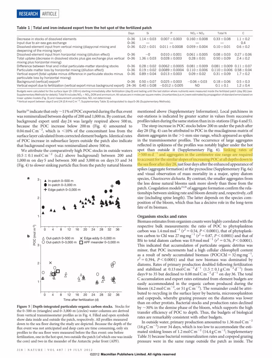
Table 1 | Total and iron-induced export from the hot spot of the fertilized patchDays Si P NO2 1 NO3 Total N C
Decrease in stocks of dissolved elements 0–36 1.14 6 0.03 0.007 6 0.003 0.160 6 0.008 0.33 6 0.08 1.1 6 0.2Input due to air–sea gas exchange 0–36 — — — — 0.4Dissolved-element input from vertical mixing (diapycnal mixing anddeepening of the mixing layer)
0–36 0.22 6 0.01 0.011 6 0.0008 0.059 6 0.004 0.10 6 0.01 0.6 6 0.2
Dissolved-element input from horizontal mixing (dilution effect) 0–36 ,0 0.010 6 0.001 0.061 6 0.005 0.08 6 0.03 0.27 6 0.06Total uptake (decrease in dissolved stocks plus gas exchange plus verticalmixing plus horizontal mixing)
0–36 1.36 6 0.03 0.028 6 0.003 0.28 6 0.01 0.50 6 0.09 2.4 6 0.2
Difference between final and initial particulate-matter standing stocks 0–36 0.28 6 0.02 0.0062 6 0.0005 0.081 6 0.009 0.081 6 0.009 0.11 6 0.07Particulate matter loss by horizontal mixing (dilution effect) 0–36 0.19 6 0.02 0.0089 6 0.0004 0.110 6 0.006 0.110 6 0.006 0.58 6 0.04Vertical export (total uptake minus difference in particulate stocks minusparticulate loss by horizontal mixing)
0–36 0.89 6 0.04 0.013 6 0.003 0.09 6 0.02 0.31 6 0.09 1.7 6 0.2
Background (vertical) export* 0–36 0.50 6 0.07 0.025 6 0.003 20.06 6 0.03 0.18 6 0.06 0.5 6 0.3Vertical export due to fertilization (vertical export minus background export) 24–36 0.40 6 0.08 20.012 6 0.005 ND 0.1 6 0.1 1.2 6 0.4
Budgets were calculated for the surface layer (0–100 m) starting immediately after fertilization (day 0) and lasting until the last station where nutrients were measured inside the fertilized patch (day 36) (seeSupplementary Methods for details). Total N includes NO2 1 NO3, DON and ammonium. All values are in moles per square metre. Uncertainties (s.e.m.) were estimated by propagation of standard errors based onlinear uptake models (Fig. 3) and measurement uncertainties. ND, not determined.*Vertical export between days 0 and 24 (0.4 mol C m22; Supplementary Table 3) extrapolated to days 0–36 (Supplementary Methods).
0 4 8 12 16 20 24 28 32 36
Time after fertilization (d)
1
2
3
PO
C (m
ol m
–2)
In-patch 0–500 mIn-patch 0–3,000 m
Out-patch 0–500 mOut-patch 0–3,000 m
Edge patch 0–3,000 m
1
2
3
0 4 8 12 16 20 24 28 32 36
Edge eddy 0–3,000 m
a
b
APF meander 0–3,000 m
Figure 5 | Depth-integrated particulate organic carbon stocks. Stocks forthe 0–500-m (triangles) and 0–3,000-m (circles) water columns are derivedfrom vertical transmissometer profiles as in Fig. 4. Filled and open symbolsshow data inside and outside the patch, respectively. All profiles measureddown to the sea floor during the study are depicted. Because the depth of theflux event was not anticipated and deep casts are time consuming, only sixprofiles to the sea floor were measured before the flux event: one beforefertilization, one in the hot spot, two outside the patch (of which one was insidethe core) and two in the meander of the Antarctic polar front (APF).
RESEARCH ARTICLE
3 1 8 | N A T U R E | V O L 4 8 7 | 1 9 J U L Y 2 0 1 2
Macmillan Publishers Limited. All rights reserved©2012

discrepancy between measured production and estimated loss rates ispartly due to three out-stations placed where there had been previousnatural blooms with comparatively low surface DIC inventories(Fig. 3a) but where much of the corresponding POC stocks hadalready sunk to subsurface layers. Furthermore, the vertical diffusioncoefficient applied14 seems to lead to an overestimation of export.Applying another, twofold-higher, diffusion coefficient for diapycnalmixing derived from microstructure profiles during EIFEX15 results intwofold-higher export values that are supported even less by directobservations of the plankton community and by POC profiles.
ConclusionsThe peak chlorophyll stock of 286 mg m22 is the highest recorded inan OIF experiment so far5 and demonstrates that, contrary to thecurrent view21, a massive bloom can develop in a mixed layer as deepas 100 m. The EIFEX results provide support for the second conditionof the iron hypothesis4, that mass sinking of aggregated cells andchains in the demise phase of diatom blooms also occurs in the openSouthern Ocean, both in natural22,23 and in artificially fertilizedblooms. Given the large sizes, high sinking rates and low respiratorylosses of aggregates from the iron-induced bloom, much of the bio-mass is likely to have been deposited on the sea floor as a fluff layer24
with carbon sequestration times of many centuries and longer.Larger-scale, longer-term OIF experiments will be required to reducethe effects of horizontal dilution and to explore further the potential ofthis technique for hypothesis testing in the fields of ecology, biogeo-chemistry and climate.
METHODS SUMMARYThe eddy was selected on the basis of satellite altimetry and surface chlorophylldistribution. Fertilization was carried out by releasing 7 t of commercial Fe(II)sulphate dissolved in 54 m3 of acidified (HCl) sea water into the ship’s propellerwash while spiralling out from a drifting buoy at 0.9-km radial intervals. Byday 14, the initial 167-km2 patch had spread and an area of 740 km2 was againfertilized with 7 t of Fe(II) sulphate, this time along east–west transects 3 km apart,from north to south in the direction of the moving patch (Fig. 1c).
The patch was located using the drifting buoy, and the photochemicalefficiency (Fv/Fm) was measured continuously with a fast-repetition-ratefluorometer. As in previous experiments, Fv/Fm was significantly higher iniron-fertilized water. Within a week, the bloom had accumulated sufficient bio-mass that additional tracers (chlorophyll concentration and continuous measure-ments of fCO2) could be used to locate the part of the patch least affected bydilution with outside water, that is, that with the highest chlorophyll concentra-tion and, in the last week, the lowest fCO2 value (Fig. 1c–f). All in-stations wereplaced inside this hot spot and care was taken to locate it with small-scale surveysbefore sampling and to keep the ship within it during sampling at each station,which generally lasted about 8 h. Some in-stations were within the patch but weresubsequently shown to have missed the hot spot and have therefore beenexcluded. For logistical reasons, the out-stations were taken in different locationsof the core relative to the direction of the moving patch, that is, ahead, behind ordiagonally opposite it.
Standard oceanographic methods and instruments15 were used to collectsamples and measure the properties of the water column. See SupplementaryInformation for details.
Received 15 November 2011; accepted 3 May 2012.
1. Sigman, D. M. Hain, M. P. & Haug, G. H. The polar ocean and glacial cycles inatmospheric CO2 concentration. Nature 466, 47–55 (2010).
2. Anderson, R. F. et al. Wind-driven upwelling in the Southern Ocean and thedeglacial rise in atmospheric CO2. Science 323, 1443–1448 (2009).
3. Martin, J. H. Glacial-interglacial CO2 changes: the iron hypothesis.Paleoceanography 5, 1–13 (1990).
4. Coale, K. H. et al. Southern Ocean iron enrichment experiment: carbon cycling inhigh- and low-Si waters. Science 304, 408–414 (2004).
5. Boyd, P. et al. Mesoscale iron-enrichment experiments 1993–2005: synthesis andfuture directions. Science 315, 612–617 (2007).
6. Cassar, N.et al. The Southern Ocean biological response to aeolian irondeposition.Science 317, 1067–1070 (2007).
7. Hamme, R. C. et al. Volcanic ash fuels anomalous plankton bloom in subarcticnortheast Pacific. Geophys. Res. Lett. 37, L19604 (2010).
8. Lampitt, R. S. et al. Material supply to the abyssal seafloor in the Northeast Atlantic.Prog. Oceanogr. 50, 27–63 (2001).
9. Abelmann, A., Gersonde, R., Cortese, G., Kuhn, G. & Smetacek, V. Extensivephytoplankton blooms in the Atlantic sector of the glacial Southern Ocean.Paleoceanography 21, PA1013 (2006).
10. Kohfeld, K. E., Le Quere, C., Harrison, S. P. & Anderson, R. F. Role of marine biologyin glacial-interglacial CO2 cycles. Science 308, 74–78 (2005).
11. The Royal Society. Geoengineering the Climate: Science, Governance andUncertainty. RS policy document 10/09 (The Royal Society, 2009).
12. Chelton, D. B., Schlax, M. G., Samelson, R. M. & de Szoeke, R. A. Global observationsof large oceanic eddies. Geophys. Res. Lett. 34, L15606 (2007).
13. d’Ovidio, F., Isern-Fontanet, J., Lopez, C., Hernandez-Garcia, E. & Garcia-Ladona, E.Comparison between Eulerian diagnostics and finite-size Lyapunov exponentscomputed from altimetry in the Algerian basin. Deep Sea Res. Part I Oceanogr. Res.Pap. 56, 15–31 (2009).
14. Hibbert, A., Leach, H., Strass, V. & Cisewski, B. Mixing in cyclonic eddies in theAntarctic Circumpolar Current. J. Mar. Res. 67, 1–23 (2009).
15. Cisewski, B., Strass, V. H., Losch, M. & Prandke, H. Mixed layer analysis of amesoscale eddy in the Antarctic Polar Front Zone. J. Geophys. Res. 113, C05017(2008).
16. Jacquet, S. H. M., Savoye, N., Dehairs, F., Strass, V. H. & Cardinal, D. D. Mesopelagiccarbon remineralization during the European Iron Fertilization Experiment. Glob.Biogeochem. Cycles 22, GB1023 (2008).
17. Paytan, A. & McLaughlin, K. The oceanic phosphorus cycle. Chem. Rev. 107,563–576 (2007).
18. Bishop, J. K. B., Wood, T. J., Davis, R. E. & Sherman, J. T. Robotic observations ofenhanced carbon biomass and export at 55u S during SOFeX. Science 304,417–420 (2004).
19. Jackson, G. A. A model of the formation of marine algal flocs by physicalcoagulation processes. Deep-Sea Res. 37, 1197–1211 (1990).
20. Riebesell, U. & Wolf-Gladrow, D. A. The relationship between physical aggregationof phytoplankton and particle flux: a numerical model. Deep-Sea Res. A 39,1085–1102 (1992).
21. de Baar, H. J. W. et al. Synthesis of iron fertilization experiments: from the iron agein the age of enlightenment. J. Geophys. Res. 110, C09S16 (2005).
22. Blain, S. et al. Effect of natural iron fertilization on carbon sequestration in theSouthern Ocean. Nature 446, 1070–1074 (2007).
23. Pollard, R. et al. Southern Ocean deep-water carbon export enhanced by naturaliron fertilization. Nature 457, 577–580 (2009).
24. Beaulieu, S. E. in Oceanography and Marine Biology. An Annual Review (eds Gibson,R. N., Barnes, M. & Atkinson, R. J.) 171–232 (Taylor & Francis, 2002).
Supplementary Information is linked to the online version of the paper atwww.nature.com/nature.
Acknowledgements We thank C. Balt, K. Loquay, S. Mkatshwa, H. Prandke, H. Rohr,M. Thomas and I. Voge for help on board. We are also grateful to U. Struck for POC andPON analyses. The altimeter products were produced by Ssalto/Duacs and distributedbyAviso with support fromCnes. We thank the captainand crewofRVPolarstern (cruiseANT XXI/3) for support throughout the cruise.
Author Contributions V.S. and C.K. wrote the manuscript. V.S. directed the experimentand C.K. carried out the budget calculations. V.H.S., P.A., M.M. and D.W.-G. contributedto the preparation of the manuscript. V.H.S., B.C., H.L. and M.L. contributed physicaldata on mixed-layer depth dynamics, eddy coherence, patch movement andtransmissometer data. N.S. provided thorium data. A.W. provided nutrient data. P.A.and J.H. provided phytoplankton and BSi data. F.D. carried out the Lagrangian analysisbasedondelayed-timealtimetry. J.M.A. andG.J.H.providedbacterial data.C.N. andR.B.provided inorganic carbon data. G.M.B., C.K. and M.M.M. provided POC and PON data.P.C. provided the iron data. S.G. and A.T. provided DOM data. I.P. and L.J.H. performedthe 14C primary production measurements and provided high-pressure liquidchromatography data. R.R. provided data on photochemical efficiency (Fv/Fm). C.K.,M.M.S. andA.T. providedChldata.U.B., E.S., O.S. and J.S. provideddataon theeddycorefrom a subsequent cruise and satellite Chl images.
Author Information Reprints and permissions information is available atwww.nature.com/reprints. The authors declare no competing financial interests.Readers are welcome to comment on the online version of this article atwww.nature.com/nature. Correspondence and requests for materials should beaddressed to V.S. ([email protected]) or C.K. ([email protected]).
ARTICLE RESEARCH
1 9 J U L Y 2 0 1 2 | V O L 4 8 7 | N A T U R E | 3 1 9
Macmillan Publishers Limited. All rights reserved©2012
�
Supplementary information
Table of contents
SI 1. Eddy properties…………………………………………….......2-6
SI 2. Eddy dynamics…………………………………………..........7-13
SI 3. Patch area evolution and dilution rates……………………...14-18
SI 4. Patch dynamics and dilution……….......................................19-22
SI 5. Iron induced and background export………..........................23-26
WWW.NATURE.COM/NATURE | 1
SUPPLEMENTARY INFORMATIONdoi:10.1038/nature

�
Supplementary Information SI 1 Properties of the eddy core and surrounding frontal meander
The eddy core and the surrounding Antarctic Polar Front (APF) meander were mapped and the
distributions of physical, chemical and biological properties measured during a quasi-synoptic
survey with a grid of 80 stations along 8 north/south transects 22 km apart from days 1 – 7, i.e.
shortly after the patch was fertilized on day 0. The ADCP derived stream function and altimeter
image from this survey are shown in Fig. 1 a and b (main text). The corresponding nutrient,
chlorophyll and diatom carbon distributions are shown in Fig. S1.1. Each station in the grid (Fig.
S1.1 c) consisted of a single CTD cast to 500 m depth which provided vertical profiles of
temperature, salinity, chlorophyll fluorescence and beam attenuation of the transmissometer.
Surface samples from the ship’s seawater intake were taken for measurements of nutrients,
chlorophyll a and microplankton composition and biomass along the survey (Fig. S1.1 b and e).
Integrated POC stocks recorded with the profiling transmissometer are depicted for the upper 500 m
and for each of the layers 0-100, 100-200, 200-300, 300-400, 400-500 m separately in Fig. S1.2.
The grid was interrupted on days 4 and 5 for one full in and two out stations, respectively.
Values for all parameters (fig. S1.1) are consistently higher in the closed eddy core and the duct
connecting it with Antarctic Zone (AZ) water in the south-eastern corner of the grid than in the
surrounding APF meander. The closed core and its origin from the AZ are clearly represented in the
high silicate and nitrate concentrations (Fig. S1.1 a-b). Note the larger gradient in silicate compared
to nitrate from core centre to the surrounding meander of the APF. Phosphate distribution within the
core is patchier than Si and N but nevertheless distinctly higher than in the meander (Fig. S1.1 c).
The same chlorophyll values, but depicted at different scales, are shown in panels d and f of Fig.
S1.1. In panel d the same scale as in Fig. 1 c and f of the main text has been used to highlight the
concentrations reached in the iron-induced bloom (see Fig. 1 c, f main text). The chlorophyll scale
used in panel e encompasses the measured values in order to magnify variability in horizontal
distribution. The orange region marked with the oval in the upper part of panel e is the patch,
crossed on grid transects 3 and 4 (from West to East), on days 3 and 4 after fertilization. The
apparent patch elongation is a sampling artefact as the patch was moving eastward with the survey.
Distribution of total diatom biomass (determined from surface samples counted under the
microscope) shown in panel f also exhibits horizontal variability which does not quite match that of
chlorophyll presumably due to differences in C/Chl ratios between iron-starved and iron-replete
cells and shifts in the ratio of total phytoplankton (i.e. including autotrophic flagellates) to diatom
carbon biomass (~ 1 in that period). Whereas the range of concentrations of chlorophyll and diatom
carbon within the eddy core is only twofold, the range of these values across the entire eddy is
about sixfold.
The scales used to depict integrated POC stocks in different layers shown in Fig. S1.2 span the
same range as the respective depth layers in Fig. 4 of the main text. Thus, maximum POC stocks
recorded in the patch would appear deep red in all these figures. The greater horizontal
homogeneity of POC stocks compared to values for Chl and diatom biomass can be explained by
variability in C/Chl ratios leading to a much smaller POC increment of the growing bloom relative
to background values and the fact that the former is an integrated value for the 100 m water column,
whereas the latter are surface values. Since the survey was carried out in a period of relatively calm
weather, accumulation of phytoplankton biomass in the surface could have led to the discrepancy.
Further, diatom C at the start of the experiment accounted for only 28% of total POC.
WWW.NATURE.COM/NATURE | 2
SUPPLEMENTARY INFORMATIONRESEARCHdoi:10.1038/nature

�
Fig. S1.1. Nutrient, chlorophyll a (Chl) and diatom biomass distribution during the eddy survey carried out from day 1
to day 7 after fertilization (14th
to 20th
February 2004). Nutrients in mmol m-3
, Chl and diatom carbon in mg m-3
.
Crosses in panel c show location of CTD stations. The grid was interrupted on days 4 and 5 for one full in-station (red
diamond in panel c) and two out-stations (black diamonds in panel c), respectively. Location of surface underway
measurements are shown as crosses in panel b (all nutrients) and e (chlorophyll). The approximate location of the patch
is marked with an elongated oval in panel e. Note minor, natural blooms to the east and south of the EIFEX patch. The
surface chlorophyll distribution on panel d is given, for comparison, using the same colour-scale as in the Figure 1 c – f
(main text). Background isopleths correspond to sea surface height anomalies (in cm) from February 18th
2004 obtained
from the Near-Real-Time Altimetry Project, Colorado Center for Astrodynamics Research (CCAR),
http://argo.colorado.edu/~realtime/gsfc_global-real-time_ssh/
WWW.NATURE.COM/NATURE | 3
SUPPLEMENTARY INFORMATIONRESEARCHdoi:10.1038/nature

�
Fig. S1.2. Integrated particulate organic carbon stock distribution in the closed core and APF meander recorded during
the same grid as Fig. 1 and S1.1. Upper left panel shows stocks for the layer integrated over 0 – 500 m and the other
panels show integrated stocks for successive 100 m layers as indicated. POC stocks are derived from beam attenuation
of a profiling transmissometer mounted on a CTD rosette calibrated with discrete POC measurements (Supplementary
Figure 5). Positions of CTD casts are indicated by the black diamonds. For comparison, the colour scales span the same
range in POC stock as the Y scales in Fig. 4 (main text) for the corresponding depth intervals. Black background
indicates values smaller than minimum values of corresponding range in Fig. 4. Background isopleths are the same as in
Fig. S1.1.
WWW.NATURE.COM/NATURE | 4
SUPPLEMENTARY INFORMATIONRESEARCHdoi:10.1038/nature
�
POC stocks integrated to 500 m depth within the eddy core ranged between 1.2 and 1.5 mol C m-2
and exhibited a greater degree of patchiness than in the surface layer due to variability in stocks in
the deeper layers. The lowest subsurface POC stocks in the core were found in the region in which
the patch was located. This region extended to the centre of the core with higher values “ahead” but
particularly “behind” the patch in the direction of flow. Since the locations of out-stations relative
to the patch were selected for logistical reasons, they were sometimes inadvertently located in these
regions of higher POC stocks. Thus, during the first survey out stations had higher particulate
stocks than the station on day -1 and the in-station on day 4.
We attribute the higher POC stocks in deeper layers to ongoing particle flux from the surface which
was remarkably patchy at local scales. This is indicated by the wide range of POC stocks in the
upper 500 m measured by successive casts taken several hours apart during the out-station on day 5
which was located in a region of higher diatom biomass in the surface (Fig. 4 k-n, main text). The
only deep cast taken at this station happened to be one with higher deep particle stocks than most of
the other casts. The higher values extended only to 1,000 m depth, stocks below 1,000 m were
similar to pre-fertilization deep stocks (Fig. 4 o-p, main text). Higher POC stocks were again
encountered in deeper layers during the last out-stations on days 33-34. High values now extended
down to 3,000 m depth, concomitant with a decline above 300 m depth compared to stocks from
day 5 (Fig. 4, main text) suggestive of sinking rates in the order of 10 - 100 m d-1
in the intervening
period. These higher stocks were absent in the previous deep cast of the out-station taken on day 25
which was evidently located in the region of low POC stocks, hence comparable to the initial
conditions of the fertilized patch and representative of most of the out-stations (Fig. 4, main text).
The tenfold higher sinking speeds of aggregates from the patch could be explained by their larger
size (compare profiles in Supplementary Fig. 6 c with d).
The patchy higher POC stocks in deep layers of the core outside the patch (Fig. S1.2.) are most
probably due to the effects of local differences in iron input by aeolian dust. The difference between
the lowest and highest out-station POC stocks between 0 – 3,000 m on days 25 and 34 respectively
is 0.62 mol C m-2
. The maximum biomass attained by these natural blooms was less than half that
attained in the hotspot. For comparison, the average value present in the upper 500 m of the hotspot
from day 20 – 36 was 1.7 ± 0.1 mol C m-2
(n = 34) and the maximum values for the 0 - 3000 m
water column on day 36 were 2.84 ± 0.04 mol C m-2
(n=3).
In striking contrast to the eddy core, POC stocks in the surrounding APF meander recorded during
the grid in the upper 500 m were consistently < 1.0 mol C m-2
. The 2 deep casts taken in the
meander (1.4 and 1.6 mol C m-2
between 0 – 3,000 m) were in the same range as the lower values
from days -1 and 25 out-patch (Fig. 5 main text). The higher 0 – 3,000 m value of 2.1 mol C m-2
obtained on day 3 was from a station located in the outer rim of the eddy and was similar to the
maximum out-patch values taken on day 35. The low POC stocks in the deep water column of the
meander are of particular interest as satellite images show that it had been the site of a bloom 2
weeks prior to our arrival (Fig. 1 g, main text). This extensive bloom along the APF had
presumably been terminated by a combination of iron and silicate limitation. Hence, the low POC
stocks indicate that biomass built up in the bloom had settled out of the water column within a two-
week period. The transmissometer profile recorded in the centre of the eddy 50 days after
fertilization during a following cruise (ANT XXI/4) indicated a lower particle load than during
EIFEX. The profile could not be accurately converted into POC because instrument drift in the
interim was not accounted for,. High uptake rates of oxygen across the sediment/water interface
were measured with a bottom lander equipped with an array of O2 sensors under the APF meander
southwest of the core during ANT XXI/4. These measurements indicated that a substantial amount
WWW.NATURE.COM/NATURE | 5
SUPPLEMENTARY INFORMATIONRESEARCHdoi:10.1038/nature

�
of POC had been previously deposited on the sea floor. Similar O2 uptake rates were found at the
sediment surface under the eddy core which we assume resulted from deposition of POC from the
iron-induced bloom. In contrast, O2 uptake rates recorded at a site in the AZ further to the south
were threefold lower.
Conclusions
a) The water mass comprising the closed core of the eddy originated from the AZ south of the APF.
b) Most properties within the core varied by <30%, indicating a coherent water mass of the same
provenance within the core.
c) However, chlorophyll concentrations, diatom biomass and deep POC stocks varied by a factor of
2 within the core but outside the patch due to processes initiated after formation of the eddy.
d) POC from the patchy natural blooms sank deep but more slowly than from the iron-induced
bloom.
e) The high POC stocks in the hotspot water column could only have come from the overlying iron-
induced bloom.
WWW.NATURE.COM/NATURE | 6
SUPPLEMENTARY INFORMATIONRESEARCHdoi:10.1038/nature

�
Supplementary Information SI 2
Eddy dynamics and dilution
Lateral stirring and eddy dilution
Lateral stirring is able to induce filaments by which water is exchanged between the core and the
exterior of eddies. This process strongly depends on the temporal variability of the velocity field
and arises on spatiotemporal scales of the order of ~10-100 km and weeks/months - relevant for the
duration and size of the fertilization. In order to minimize the dilution of the fertilized patch due to
the lateral stirring, the eddy was chosen on the basis of two dynamical characteristics observed from
altimetry before and during the cruise: (i) an extremely slow temporal variability and (ii) a very
weak interaction with the other nearby eddies. These characteristics persisted during the cruise. In
order to confirm quantitatively that these characteristics implied a weak dilution of the eddy core,
we performed a post-cruise Lagrangian analysis based on altimetry data1.
The analysis was based on the calculation of Okubo-Weiss parameter, finite-size Lyapunov
exponent2 and particle trajectories. These tools applied to altimetry have been shown to describe in
a robust way the filamentation of mesoscale eddies by lateral stirring, reproducing filaments well
matched in chlorophyll and sea surface temperature images1,3,4
.
The Okubo-Weiss parameter is routinely used to localize eddies from snapshots of the velocity
field. This diagnostic provides the dominance of the strain rate in respect to vorticity and therefore
marks with negative values regions occupied by eddies. Calling u and v respectively the
longitudinal and zonal component of the velocities, one can measure the normal and shear
components of the strain Sn and Ss and the vorticity ω:
Ss=∂v/∂x+∂u/∂y
Sn=∂u/∂x-∂v/∂y
ω=∂v/∂x-∂u/∂y
Then the Okubo-Weiss parameter W is
W= Sn2+Ss
2-ω2
The Lyapunov exponent is computed at point x and time t by calculating the separation of
trajectories initialized nearby backward in time. This is achieved by integrating the altimetry-
derived geostrophic velocities. Calling δ0 and δ respectively the initial and final trajectories'
separation and Δt the time needed to reach the separation δ, the local Lyapunov exponent λ is
obtained by assuming an exponential separation of the nearby trajectories:
δ = δ0 exp(λ . ∆t)
Inverting this relation one can find the Lyapunov exponent as:
λ (x,t)= (1/∆t) log(δ /δ0)
In physical terms, the value of the Lyapunov exponent indicates the exponential stretching that a
parcel of water undergoes while it is advected. Maxima of Lyapunov exponents correspond to sharp
WWW.NATURE.COM/NATURE | 7
SUPPLEMENTARY INFORMATIONRESEARCHdoi:10.1038/nature
�
fronts of tracers that have been passively advected for timescales of the order of 1/λ (refs.1,3,5,6).
The combination of Okubo-Weiss and Lyapunov exponents has been shown to be a powerful tool
for detecting the position of mesoscale eddies and the effect of these eddies on advected tracers3.
Here we used this approach to identify the fertilized eddy and the fronts defining the boundaries of
the eddy core. The analysis was based on geostrophic velocities produced by AVISO from satellite
sea surface height anomalies7 and RIO-05 mean dynamic topography
8 that were linearly
interpolated in space and time when needed. Integration of the velocity was done with a Runge-
Kutta integrator of fourth order. Details of the calculation can be found in refs. 2 and 3.
A map of Okubo-Weiss parameter and local Lyapunov exponent for the first day after fertilization
(14 February 2004) is shown in Figs. S2.1 and S2.2, where a white square indicates the centre of the
fertilized patch. The Okubo-Weiss map reveals the fertilized eddy as the dominant recirculating
structure (in terms of vorticity vs. strain signature) in the mesoscale field. The lines of Lyapunov
maximal values (corresponding to fronts that separate water masses of different origin) show this
eddy as the one with the most regular and closed core. This difference is remarkable when the core
of the fertilized eddy is compared to the core of the anticyclone at 3.7°E, 49.2°S which has a
relatively strong Okubo-Weiss signature but lacks an isolated core, appearing in the Lyapunov map
only as a lobe of the Antarctic Circumpolar Current. This is a consequence of both a stronger
vorticity and weaker temporal dynamics of the fertilized eddy in comparison to the other eddies of
the region. The fertilized eddy contains a core centered at 2.25°E, 49.6°S with a diameter of about
60 km, encircled by a peripheral region with a width of ~20 km. A meander of the Antarctic
Circumpolar Current is visible around the eddy. The South-East sector of the core is shifted South-
East in respect to the boundary detected by the Okubo-Weissparameter, otherwise the core is fairly
aligned with Okubo-Weiss isolines. The core is characterized by a very weak stretching rate
(Lyapunov exponents less than 0.1 d-1
) and is delimited by Lyapunov exponents in excess of 0.3 d-1
.
We recall that the intensity of Lyapunov values indicate the timescale over which a tracer contour
aligns to the line of maximal Lyapunov exponents3. For the case of the core boundaries, this
corresponds to 1/0.3≈3 days. The core appears to exchange water only through a thin duct a few
kilometers wide, stemming from the southern edge of the core and extending westward. This
analysis is consistent with the numerical advection of a test tracer initially located inside the eddy at
the day of fertilization (Fig. S2.3).
These results from delayed-time altimetry strongly support the pre- and in-cruise analysis based on
near-real-time altimetry, confirming a weak perturbation of the fertilized eddy by the other eddies
and an almost closed structure of the eddy core. Note also that the south-eastward shift of the
Lagrangian core (i.e., of the water mass most isolated inside the eddy) relative to the position of the
centre of the sea surface height anomaly (or Okubo-Weiss minimum) balanced the inadvertent off-
centre error during the placement of the fertilized patch.
WWW.NATURE.COM/NATURE | 8
SUPPLEMENTARY INFORMATIONRESEARCHdoi:10.1038/nature

�
Figure S2.1. Eddy detection. Okubo-Weiss parameter calculated from altimetry-derived
geostrophic velocity at the beginning of the experiment (14th February 2004). The Okubo-Weiss
parameter identifies eddies as regions where vorticity dominates the strain rate. The white square
corresponds to the centre of the fertilized patch.
WWW.NATURE.COM/NATURE | 9
SUPPLEMENTARY INFORMATIONRESEARCHdoi:10.1038/nature

�
Figure S2.2. Fronts induced by lateral stirring. Lyapunov exponent calculated from altimetry-
derived geostrophic velocity at the beginning of the experiment (14th February 2004). The
Lyapunov exponent (d-1
) measures the stretching of an advected parcel of fluid. Lines of maxima of
Lyapunov exponent indicate transport barriers induced by the lateral stirring. These lines can be
interpreted as fronts between water masses of different origins (see text for an interpretation of the
Lyapunov values). The white square corresponds to the centre of the fertilized patch. Note that the
fertilized eddy is the only mesoscale structure in the region with a core well bounded by transport
barriers.
Core dynamics and dilution rate
In order to quantify the dilution of the eddy core during the experiment, we reconstructed the
evolution of the eddy content by numerically measuring the advection of a test tracer initially
placed in the region of negative Okubo-Weiss values. The advection was done by integration of
altimetry-derived geostrophic velocities, linearly interpolating in space and time when needed. The
Okubo-Weiss signature of the eddy was tracked for each day. Some snapshots of the advected patch
are shown in Fig. S2.3. By reconstructing the origin of the eddy content for each day, we estimated
the dilution rate as the fraction of the initial eddy content that was exchanged1. The fraction of the
tracer located inside the eddy at the day of fertilization and still present inside the eddy in the
following days is plotted in Fig. S2.4. As expected by the eddy structure revealed by the Lyapunov
analysis, there is a sharp decrease during the first days, when the content of the eddy periphery is
rapidly ejected (8-10 days). This part of the eddy accounts for 20-25% of the original content of the
eddy and corresponds equivalently to a dilution rate of 2-3%/day. The dilution proceeds then at a
much slower speed (about 0.1%/day) when the content of the eddy core starts to be eroded. We thus
WWW.NATURE.COM/NATURE | 10
SUPPLEMENTARY INFORMATIONRESEARCHdoi:10.1038/nature

�
concluded that during the experiment (38 days) the eddy core may have been contaminated by the
intrusion of surrounding waters by less than 10%.
Figure S2.3. Lagrangian evolution of the eddy content. Advection of a numerical tracer (black
dots) and Okubo-Weiss parameter (color scale as in Fig. S1.1).The tracer is initialized inside the
fertilized eddy on the 13th of February 2004. The panels show the evolution of the tracer and the
Okubo-Weiss field at day 0, 2, 8, and 16 from fertilization (i.e., February 13, 15, 21 and 1st of
March 2004, from left to right and from top to bottom). Note that already at the second day most of
the tracer contained in the eddy periphery is ejected. After eight days the tracer shadows the
structure unveiled by the Lyapunov exponent analysis. After sixteen days the core is still mostly
preserved, being only eroded by a very thin filament. Spatial structures and timescales are in
excellent agreement with results from the Lyapunov analysis.
WWW.NATURE.COM/NATURE | 11
SUPPLEMENTARY INFORMATIONRESEARCHdoi:10.1038/nature

�
Figure S2.4. Eddy dilution. The plot shows the fraction of the original content of the EIFEX eddy
(defined as the region with negative Okubo-Weiss) that remained inside the eddy as a function of
time from 12th
February 2004. The eddy region is defined as a circle of 100 km centered over the
eddy centre (computed as the minimum of the Okubo-Weiss parameter at each day). In agreement
with the Lyapunov analysis (Fig. S2.2) and particle trajectories (Fig. S2.3), the eddy dilution occurs
in two steps: a fast ejection of the periphery (days 5-10, 20-25% of the eddy content) followed by a
much slower erosion of the core (about 2-3% of the eddy, or 3-4% of the core, in 20 days).
References for SI 2
1. Lehahn, Y., d'Ovidio, F., Lévy, M. & Heifetz, E. Stirring of the northeast Atlantic spring bloom:
A Lagrangian analysis based on multisatellite data. J. of Geophys. Res. Vol 112, C08005 (2007).
2. d’Ovidio, F., Fernandez, V., Hernandez-Garcia, E. & Lopez, C. Mixing structures in the
Mediterranean Sea from finite-size Lyapunov exponents. Geophys. Res. Lett. Vol 31 , L17203
(2004).
3. d'Ovidio, F., Isern-Fontanet, J., López, C., García-Ladona, E. & Hernández-García, E.
Comparison between Eulerian diagnostics and the finite-size Lyapunov exponent computed from
altimetry in the Algerian Basin. Deep Sea Res. I 56, 15-31 (2009).
WWW.NATURE.COM/NATURE | 12
SUPPLEMENTARY INFORMATIONRESEARCHdoi:10.1038/nature

�
4. Beron-Vera, F. J., Olascoaga, M. J. & and Goni, G. J. Oceanic mesoscale eddies as revealed by
Lagrangian coherent structures. Geophys. Res. Lett. 35, L12603 (2008).
5. Boffetta, G., Lacorata, G., Redaelli, G. & Vulpiani, A. Detecting barriers of transport: a review of
different techniques. Physica D 159, 58-70 (2001).
6. Shadden, S.C., Lekien, F. & Marsden, J. E. Definition and properties of Lagrangian coherent
structures from finite-time Lyapunov exponents in two-dimensional aperiodic flows. Physica D
212, 271-304 (2005).
7. Ssalto/Duacs User handbook (M)SLA and (M)ADT near-real time and delayed time products.
CLS-DOS-NT-06.034 (2006)
8. Rio, M.-H., Poulain, P.-M., Pascual, A., Mauri, E., Larnicol, G. & Santoleri, R. A Mean Dynamic
Topography of the Mediterranean Sea computed from altimetric data, in-situ measurements and
a general circulation model. J. Mar. Sys. 65, 484-508 (2007).
WWW.NATURE.COM/NATURE | 13
SUPPLEMENTARY INFORMATIONRESEARCHdoi:10.1038/nature
�
Supplementary Information SI 3 Patch area evolution and dilution rates
Patch area
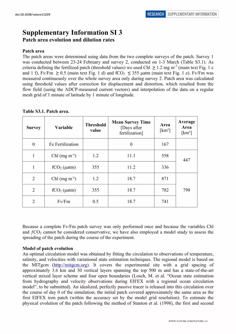
The patch areas were determined using data from the two complete surveys of the patch. Survey 1
was conducted between 23-24 February and survey 2, conducted on 1-3 March (Table S3.1). As
criteria defining the fertilized patch (threshold values) we used Chl ≥ 1.2 mg m-3
(main text Fig. 1 c
and 1 f), Fv/Fm ≥ 0.5 (main text Fig. 1 d) and fCO2 ≤ 355 µatm (main text Fig. 1 e). Fv/Fm was
measured continuously over the whole survey area only during survey 2. Patch area was calculated
using threshold values after correction for displacement and distortion, which resulted from the
flow field (using the ADCP-measured current vectors) and interpolation of the data on a regular
mesh grid of 1 minute of latitude by 1 minute of longitude.
Table S3.1. Patch area.
Survey Variable
Threshold
value
Mean Survey Time
[Days after
fertilization]
Area
[km²]
Average
Area
[km²]
0 Fe Fertilization 0 167
1 Chl (mg m-³) 1.2 11.1 558
1 fCO2 (µatm) 355 11.2 336
447
2 Chl (mg m-³) 1.2 18.7 871
2 fCO2 (µatm) 355 18.7 782
2 Fv/Fm 0.5 18.7 741
798
Because a complete Fv/Fm patch survey was only performed once and because the variables Chl
and ƒCO2 cannot be considered conservative, we have also employed a model study to assess the
spreading of the patch during the course of the experiment.
Model of patch evolution
An optimal circulation model was obtained by fitting the circulation to observations of temperature,
salinity, and velocities with variational state estimation techniques. The regional model is based on
the MITgcm (http://mitgcm.org). It covers the experimental site with a grid spacing of
approximately 3.6 km and 30 vertical layers spanning the top 500 m and has a state-of-the-art
vertical mixed layer scheme and four open boundaries (Losch, M. et al. “Ocean state estimation
from hydrography and velocity observations during EIFEX with a regional ocean circulation
model”, to be submitted). An idealized, perfectly passive tracer is released into this circulation over
the course of day 0 of the simulation; the initial patch covered approximately the same area as the
first EIFEX iron patch (within the accuracy set by the model grid resolution). To estimate the
physical evolution of the patch following the method of Stanton et al. (1998), the first and second
WWW.NATURE.COM/NATURE | 14
SUPPLEMENTARY INFORMATIONRESEARCHdoi:10.1038/nature

�
moments (relative to the centre of mass) of the passive tracer distribution are calculated for every
4th
hour of the model simulation. The squared mean radial distance of a tracer particle from the
centre of mass is estimated from these moments under the assumption of a Gaussian distribution of
the tracer concentrations as m2/m0 -m12/m0
2, where mi is the i'th moment (Fig. S3.1). The
assumption of a Gaussian distribution is, however, not valid for the first days of the integration
when the patch concentration is nearly homogeneous and has a sharp edge.
Figure S3.1. Temporal development of the patch area as estimated by the model-calculated
squared radial distance multiplied by π (red dots) and patch areas obtained from the surveys of
ƒCO2 (blue dots), Fv/Fm (orange dots) and Chl (green dots). The different parameters used to
define patch boundaries leads to the scatter in patch areas obtained at a given time, however, they
have a minor effect on the estimation of temporal developments of the patch sizes.
Using the same model data for a regression of the squared radial distance versus time in seconds
yields a slope of 113 which after division by 2 translates into a horizontal diffusivity of 56 m2 s
-1.
Dilution rates
From the temporal evolution of the patch area (A) the dilution rate for the whole patch (γ) can be
estimated by assuming that the patch area increases at a constant rate γ = A-1
dA/dt.
Spreading rates are obtained by fitting observations of patch area to straight lines through each pair
of points and for the sake of consistency using a linear regression (Fig. S3.1). The patch area
WWW.NATURE.COM/NATURE | 15
SUPPLEMENTARY INFORMATIONRESEARCHdoi:10.1038/nature

�
estimated from Fv/Fm is related to the initially fertilised area. Fv/Fm reacted to the addition of iron
within hours and afterwards remained at approximately constant high values until the end of the
experiment. From all variables measured in the field, Fv/Fm thus was the most direct and
`conservative´ indicator of the iron supply.
The obtained dilution rates vary between 0.058 d-1
and 0.106 d-1
(Table S3.2). Because this range
results from combining conservative and non-conservative properties, it likely overestimates the
error of the dilution rate that can be determined from our assessment. Closest to each other are the
dilution rates determined from the model (0.064 d-1
) and from combining the fertilised area and the
Fv/Fm survey (0.068 d-1
). Using the horizontal diffusivity Kh = 56 m2
s-1
implied by the model (see
caption Figure S5.1) to estimate the dilution rate as γ = 2 Kh / σ2, where σ2
is the squared radial
distance (12.4 km) yields 0.064 d-1
.
Table S3.2. Patch dilution rates (rates are in d-1
)
Model
Fv/Fm
Fertilization
→
Survey 2
Chl
Survey 1
→
Survey 2
ƒCO2
Survey 1
→
Survey 2
0.064 0.068 0.058 0.106
These patch dilution rates are a factor 6 – 12 higher than the dilution rates estimated for the core
water mass of the eddy (Figs. S.3.2 and S3.3) due to mixing with water from the outside, either
based on a horizontal diffusivity 87 m2
s-1
derived from the observed gradual warming of the eddy
core1 (0.008 d
-1, Fig. S3.3) or 0.009 d
-1 determined by lateral stirring derived from altimetry-based
eddy dynamics (Supplementary Information SI.2, Fig. S2.4). Note that while the horizontal
diffusivities determined for the patch (56 m2
s-1
) and for the eddy2 (87 m
2 s
-1) differ by less then a
factor of 2, the difference in dilution rates (about one order of magnitude) results from horizontal
scales being roughly three times larger for the eddy compared to the fertilized patch.
WWW.NATURE.COM/NATURE | 16
SUPPLEMENTARY INFORMATIONRESEARCHdoi:10.1038/nature
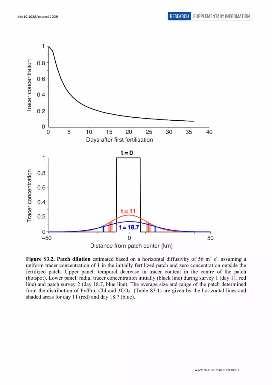
�
Figure S3.2. Patch dilution estimated based on a horizontal diffusivity of 56 m2 s
-1 assuming a
uniform tracer concentration of 1 in the initially fertilized patch and zero concentration outside the
fertilized patch. Upper panel: temporal decrease in tracer content in the centre of the patch
(hotspot). Lower panel: radial tracer concentration initially (black line) during survey 1 (day 11, red
line) and patch survey 2 (day 18.7, blue line). The average size and range of the patch determined
from the distribution of Fv/Fm, Chl and ƒCO2 (Table S3.1) are given by the horizontal lines and
shaded areas for day 11 (red) and day 18.7 (blue).
WWW.NATURE.COM/NATURE | 17
SUPPLEMENTARY INFORMATIONRESEARCHdoi:10.1038/nature
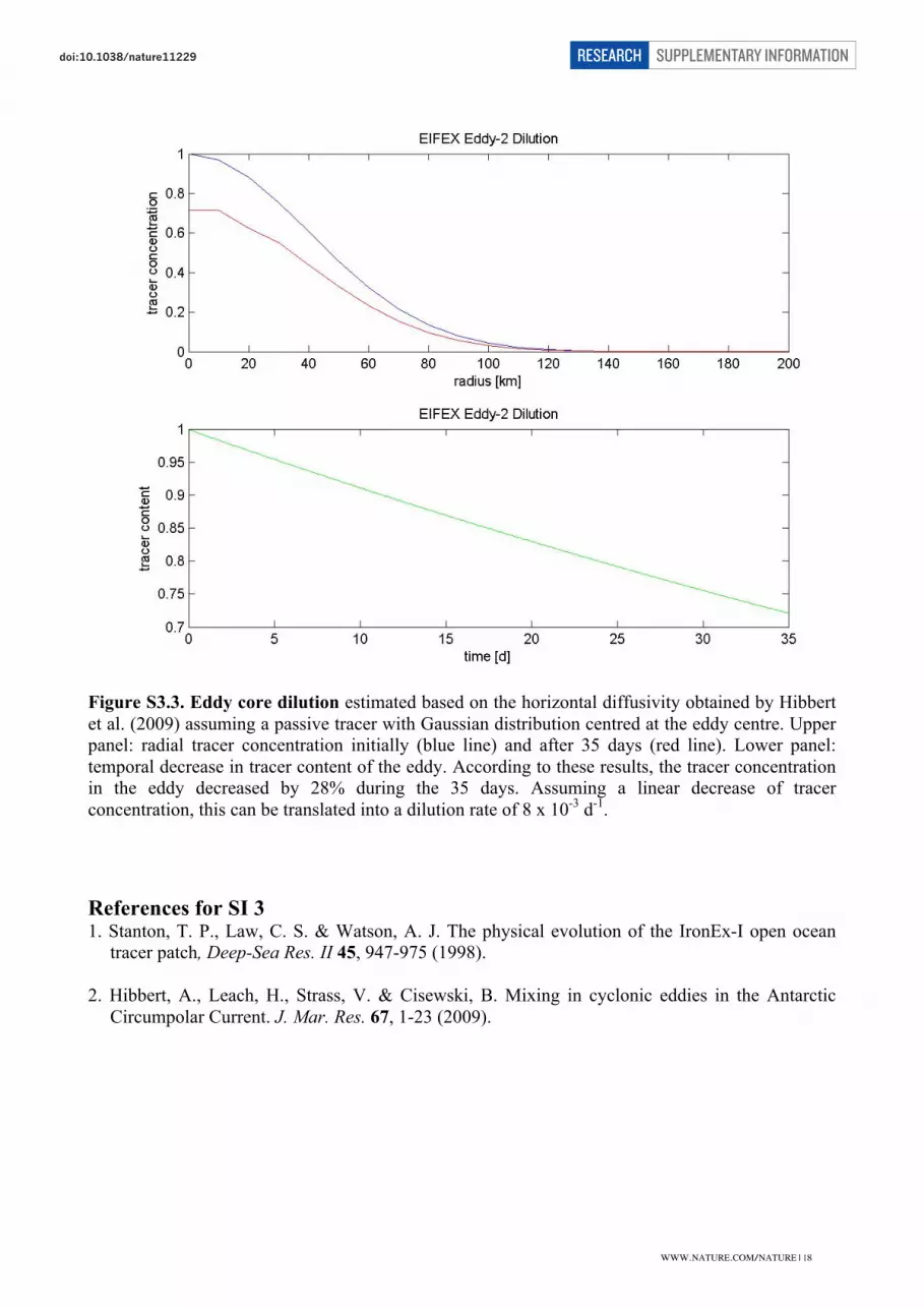
�
Figure S3.3. Eddy core dilution estimated based on the horizontal diffusivity obtained by Hibbert
et al. (2009) assuming a passive tracer with Gaussian distribution centred at the eddy centre. Upper
panel: radial tracer concentration initially (blue line) and after 35 days (red line). Lower panel:
temporal decrease in tracer content of the eddy. According to these results, the tracer concentration
in the eddy decreased by 28% during the 35 days. Assuming a linear decrease of tracer
concentration, this can be translated into a dilution rate of 8 x 10⁻³
d-1
.
References for SI 3 1. Stanton, T. P., Law, C. S. & Watson, A. J. The physical evolution of the IronEx-I open ocean
tracer patch, Deep-Sea Res. II 45, 947-975 (1998).
2. Hibbert, A., Leach, H., Strass, V. & Cisewski, B. Mixing in cyclonic eddies in the Antarctic
Circumpolar Current. J. Mar. Res. 67, 1-23 (2009).
WWW.NATURE.COM/NATURE | 18
SUPPLEMENTARY INFORMATIONRESEARCHdoi:10.1038/nature

�
Supplementary Information SI 4 Patch dynamics and dilution
The same Lagrangian scheme employed in SI 2 is used to estimate the dilution of the fertilized
patch under the effect of filamentation (due to lateral stirring) and diffusion (due to small-scale
turbulence). In order to achieve this, we advect Lagrangian particles initially equally spaced at
0.001 deg. with the altimetry-derived velocity field plus a random noise with an intensity
corresponding to a diffusivity of 56 m2 s
-1. The advantage of this method is that no hypothesis is
made on the shape that the patch maintains during its evolution. Some snapshots of the patch
evolution, computed as the density of Lagrangian particles over a grid of 0.06 deg intervals are
shown in Fig. S4.1. Particle number and grid size are chosen so that the particle density fluctuations
over the grid due to the representation of diffusivity in terms of noise are negligible and so that
patch filamentation can be fully resolved. The particle density is normalized so that a density of 1
corresponds to the undiluted fertilized patch. In agreement with the Lyapunov analysis of the eddy
core evolution, stretching is very weak in the fertilized region and the patch maintains a regular and
isotropic shape during its evolution. A weak stretching can be seen in Fig. S4.1 (lower right panel),
when the patch starts to be skewed and the hotspot is a few km off from the eddy center. For each
time of the simulation we measured the patch dispersion computing the standard deviation of
particles composing the patch (white circles in Fig. S4.1). Figure S4.2 shows, in blue, the standard
deviation of particle distribution, as a function of the days since fertilization. If only diffusion is
active, the problem of a patch evolution in two dimensions has a well known analytical solution
corresponding to:
Therefore, for this case the patch dispersion has a linear relation with the time:
This Gaussian behaviour is shown by the red line in Fig. S4.2. The modelled patch deviates from
the linear relation because of the presence of stirring, which stretches and skews the patch and
amplifies the diffusivity due to small-scale turbulence. The dispersion is clearly super-diffusive
after 35 days, when the patch develops some skewness and the Gaussian approximation for the
standard deviation breaks down. The evolution of the hotspot (i.e., the maximal concentration of the
patch) is indicated in Fig. S4.3. Again, the red line represents the dilution that is expected for a
patch whose Gaussian evolution is determined by diffusion alone. In this case the maximum or
hotspot concentration evolves as:
The hotspot (blue line in Fig. S4.3) closely follows a Gaussian behaviour and is less affected by
stirring than the standard deviation. The model estimates the hotspot dilution is 26%, 13%, 9.5%
and 0.075% after respectively 10, 20, 30, and 40 days. Also note that if the patch had been released
in a region of more intense stirring, such as at the eddy periphery, the filamentation process would
have started to dominate over the Gaussian behaviour from the beginning of the experiment, and the
patch would have been dispersed after a few days.
WWW.NATURE.COM/NATURE | 19
SUPPLEMENTARY INFORMATIONRESEARCHdoi:10.1038/nature
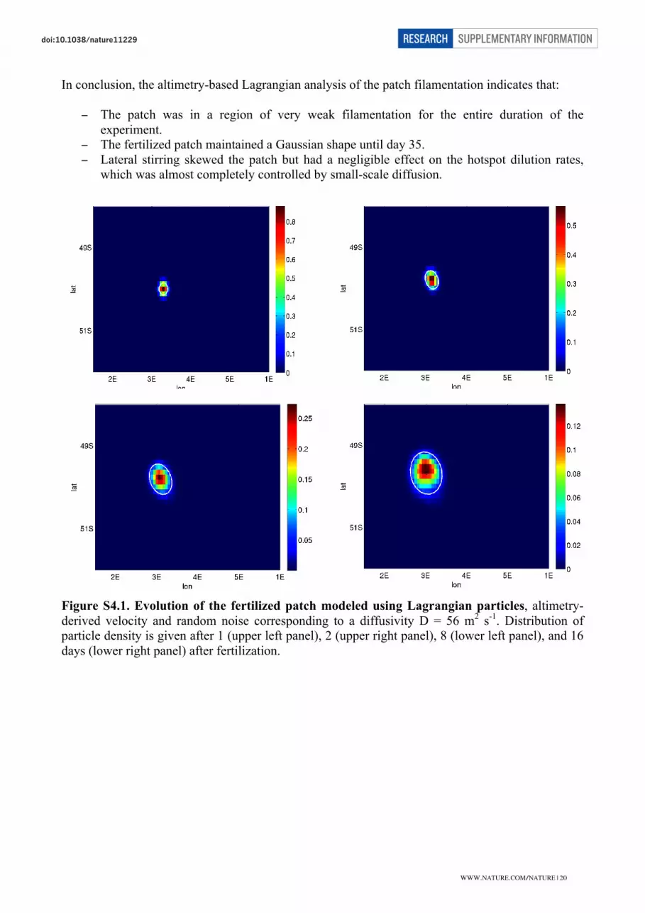
�
In conclusion, the altimetry-based Lagrangian analysis of the patch filamentation indicates that:
− The patch was in a region of very weak filamentation for the entire duration of the
experiment.
− The fertilized patch maintained a Gaussian shape until day 35.
− Lateral stirring skewed the patch but had a negligible effect on the hotspot dilution rates,
which was almost completely controlled by small-scale diffusion.
Figure S4.1. Evolution of the fertilized patch modeled using Lagrangian particles, altimetry-
derived velocity and random noise corresponding to a diffusivity D = 56 m2 s
-1. Distribution of
particle density is given after 1 (upper left panel), 2 (upper right panel), 8 (lower left panel), and 16
days (lower right panel) after fertilization.
WWW.NATURE.COM/NATURE | 20
SUPPLEMENTARY INFORMATIONRESEARCHdoi:10.1038/nature
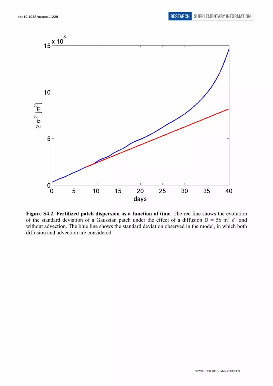
�
Figure S4.2. Fertilized patch dispersion as a function of time. The red line shows the evolution
of the standard deviation of a Gaussian patch under the effect of a diffusion D = 56 m2 s
-1 and
without advection. The blue line shows the standard deviation observed in the model, in which both
diffusion and advection are considered.
WWW.NATURE.COM/NATURE | 21
SUPPLEMENTARY INFORMATIONRESEARCHdoi:10.1038/nature

�
Figure S4.3. Evolution of the hotspot particle concentration as a function of time. The red line
shows the evolution of the maximum concentration of a Gaussian patch under the effect of a
diffusivity D = 56 m2 s
-1 alone. The blue line shows the maximum (hotspot) concentration observed
in the model, in which both diffusion and advection are considered.
WWW.NATURE.COM/NATURE | 22
SUPPLEMENTARY INFORMATIONRESEARCHdoi:10.1038/nature
�
Supplementary Information SI 5 Iron-induced and background export
Export from natural vs. artificial blooms
The Antarctic Zone is the least productive belt of the ACC with Chl concentrations typically <0.2
mg Chl m-3
. Hence, the concentrations prevailing in the eddy core in the region of the patch prior to
fertilization (~0.7 mg Chl m-3
) are elevated and the patches in the core with twofold higher
concentrations can be accorded the status of minor blooms. The Antarctic Polar Front on the other
hand is the most productive zone of the ACC presumably due to dust deposition caused by higher
rainfall levels along this weather front. Ship-borne observations indicate that precipitation events
tend to be local and short which would explain the patchiness within the eddy core. Further to the
West, dust input from iceberg melting can be a significant source of iron but icebergs were absent
in the EIFEX eddy.
Our observations indicate that export from the 3 biomass levels encountered during EIFEX: the 0.7
Chl mg m-3
pre-fertilization situation, the >1.0 mg minor, natural blooms in the eddy core and the
2.8 mg Chl m-3
reached at the peak of the EIFEX bloom varied with regard to the rate of sinking
and the depths reached by the sinking particles prior to remineralisation. The common feature is
that the carbon missing from the surface layer was not respired within it but exported to
successively deeper layers depending on the biomass levels of the diatom stocks. Apparently the
surface regenerating community has an upper threshold of retention beyond which “excess” POC,
contributed by diatoms in the presence of silicate, eventually settles out together with the iron on
which the production was based. This is consistent with the short life-time of iron introduced from
dust or from shelf sediments to the surface layer1,2
and implies that, at least in the case of diatoms,
the iron is lost together with organic matter at high C:Fe ratios3.
Similarly, there will also be an upper threshold on the ability of the subsurface heterotrophic
community to respond to an increase in the food supply dictated by their respective intrinsic growth
rates. Thus, export from lower biomass levels was respired in the upper few 100 m within days as
the accumulation rate was <10 % of export. In contrast, sinking POC from the intermediate biomass
level (natural blooms) had a much longer life-time (weeks) in the water column. Vertical flux from
these minor blooms was slower than from the EIFEX bloom, presumably because the lower
concentrations of the former resulted in smaller aggregates. Nevertheless, the bulk of biomass from
these natural diatom blooms apparently also sank deep. Export from the EIFEX bloom lost an even
smaller percentage of POC to respiration underway. Similarly, the extensive bloom present in the
APF meander prior to our arrival had not only disappeared from the surface, but from the entire
water column some 2 weeks later when the grid was conducted (Fig. S1.2). It is likely that the entire
1.8 mol C m-2 which accumulated in the water column during EIFEX sank out of it within weeks of
our departure. In conclusion, subsurface respiration of sinking particles increases with the
magnitude of flux up to a threshold beyond which the bulk of the flux settles out of the water
column. Testing this hypothesis and estimating the response rates of the subsurface heterotrophic
community to increasing flux could be one of the foci of future experiments.
Our observations are consistent with the conclusions drawn from excess barium profiles taken
during EIFEX4 which is a proxy for carbon remineralisation rates. The authors estimated rates
ranging between 14 and 96 mg C m-2
d-1
(1.2 – 8 mmol) for the 150 – 1000 m water column inside
and outside the patch whereby the highest values were recorded on days 28 in-patch (at the start of
the iron induced flux) and on day 34 out-patch (in the site of the natural bloom). Interestingly, rates
WWW.NATURE.COM/NATURE | 23
SUPPLEMENTARY INFORMATIONRESEARCHdoi:10.1038/nature
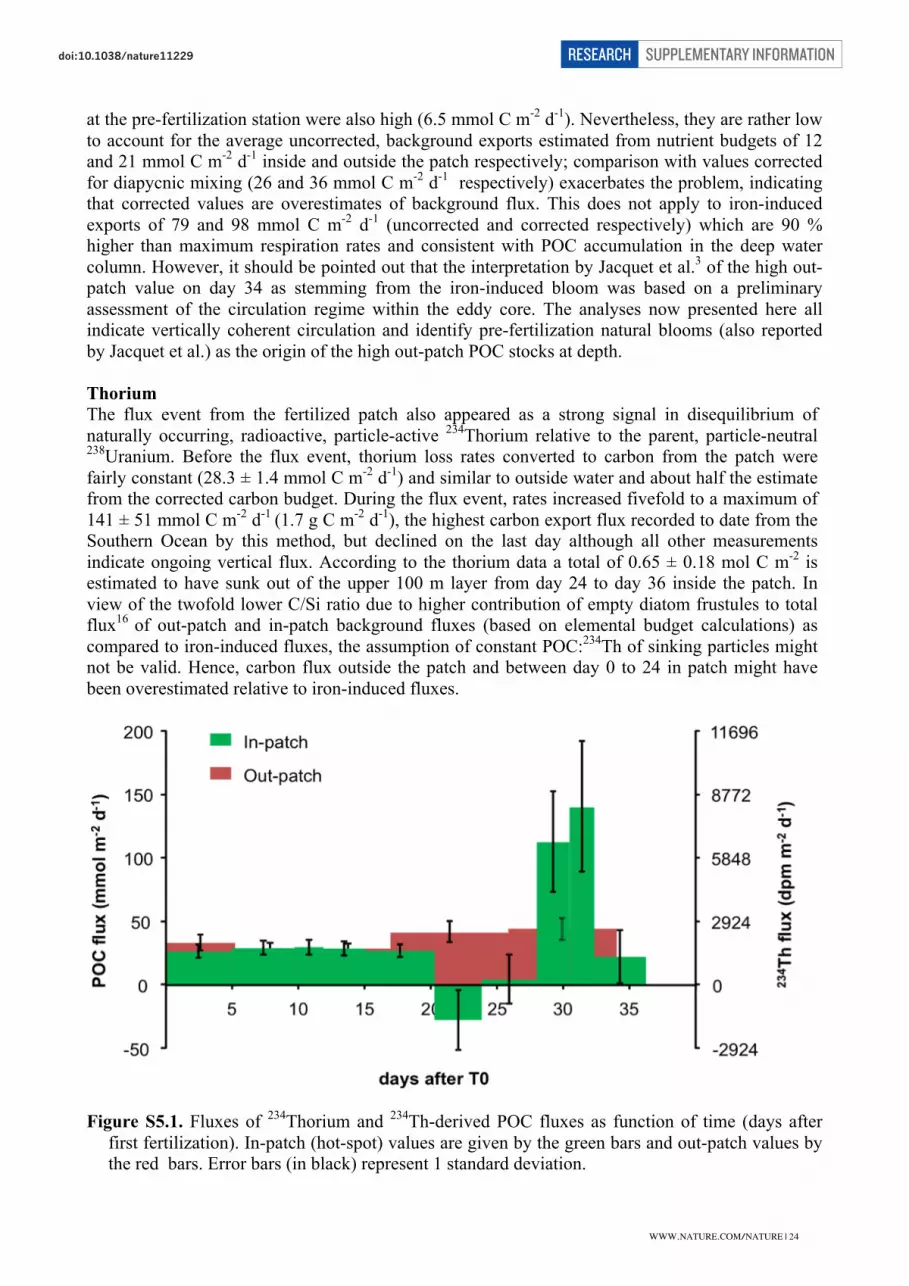
�
at the pre-fertilization station were also high (6.5 mmol C m-2
d-1
). Nevertheless, they are rather low
to account for the average uncorrected, background exports estimated from nutrient budgets of 12
and 21 mmol C m-2
d-1
inside and outside the patch respectively; comparison with values corrected
for diapycnic mixing (26 and 36 mmol C m-2
d-1
respectively) exacerbates the problem, indicating
that corrected values are overestimates of background flux. This does not apply to iron-induced
exports of 79 and 98 mmol C m-2
d-1
(uncorrected and corrected respectively) which are 90 %
higher than maximum respiration rates and consistent with POC accumulation in the deep water
column. However, it should be pointed out that the interpretation by Jacquet et al.3 of the high out-
patch value on day 34 as stemming from the iron-induced bloom was based on a preliminary
assessment of the circulation regime within the eddy core. The analyses now presented here all
indicate vertically coherent circulation and identify pre-fertilization natural blooms (also reported
by Jacquet et al.) as the origin of the high out-patch POC stocks at depth.
Thorium
The flux event from the fertilized patch also appeared as a strong signal in disequilibrium of
naturally occurring, radioactive, particle-active 234
Thorium relative to the parent, particle-neutral 238
Uranium. Before the flux event, thorium loss rates converted to carbon from the patch were
fairly constant (28.3 ± 1.4 mmol C m-2
d-1
) and similar to outside water and about half the estimate
from the corrected carbon budget. During the flux event, rates increased fivefold to a maximum of
141 ± 51 mmol C m-2
d-1
(1.7 g C m-2
d-1
), the highest carbon export flux recorded to date from the
Southern Ocean by this method, but declined on the last day although all other measurements
indicate ongoing vertical flux. According to the thorium data a total of 0.65 ± 0.18 mol C m-2
is
estimated to have sunk out of the upper 100 m layer from day 24 to day 36 inside the patch. In
view of the twofold lower C/Si ratio due to higher contribution of empty diatom frustules to total
flux16
of out-patch and in-patch background fluxes (based on elemental budget calculations) as
compared to iron-induced fluxes, the assumption of constant POC:234
Th of sinking particles might
not be valid. Hence, carbon flux outside the patch and between day 0 to 24 in patch might have
been overestimated relative to iron-induced fluxes.
Figure S5.1. Fluxes of 234
Thorium and 234
Th-derived POC fluxes as function of time (days after
first fertilization). In-patch (hot-spot) values are given by the green bars and out-patch values by
the red bars. Error bars (in black) represent 1 standard deviation.
WWW.NATURE.COM/NATURE | 24
SUPPLEMENTARY INFORMATIONRESEARCHdoi:10.1038/nature

�
C/Fe ratios of the EIFEX bloom
The C/Fe ratio of 13,000 ± 1000 presented in the main text is an underestimate for the following
reasons: a) Fv/Fm values did not change until the end of the experiment implying that hotspot
phytoplankton had not yet reached iron limitation; b) the iron added during the second fertilization
remained in the water column as dissolved iron for several weeks (Fig. S5.2) and the increase in
dissolved iron concentrations below 100 m depth (Fig. S5.2) indicates that much of the iron from
the second fertilization was lost through physical processes; c) enhanced primary production and
carbon uptake and fluxes continued after we left the eddy.
Figure S5.2. Dissolved iron concentrations as function of time (days after first fertilization).
Average surface layer (0-100 m) in-patch values are given by the filled circles and out-patch values
by the open circles. Mean concentrations in deeper layers (120-150 m) are shown by grey
diamonds. Theoretical dissolved iron curve (dotted line) shows the dissolved iron evolution in the
hot-spot assuming no uptake and a horizontal diffusivity of 56 m2s
-1. The high value at 150 m on
day 35 is probably an outlier.
We employed an alternative approach to estimating the C/Fe ratio of biomass built up by
fertilization: We estimated the total amount of chlorophyll in the 100 m surface layer of the patch
after it had spread to 798 km2 during the second mapping on days 17 – 20 using 1.0 mg Chl m
-3 as
the outer boundary of the patch. If, in a thought experiment, this amount is compressed into the 167
km2 area initially fertilized, we obtain a standing stock of 900 mg Chl m
-2 which is three times the
stock measured in the hotspot a day later. POC in the hotspot water column integrated to 3,000 m
depth continued increasing at the same rate until the end of the experiment, implying that the rate of
biomass accumulation did not change. We extrapolate the increase from day 0 – 20 to day 36 and
obtain a hypothetical standing stock in the initial patch of 1600 mg Chl m-2
. Converted into POC
using the C/Chl (mg/mg) ratio of 32 we obtain 50 g C m-2
or 4.2 mol C m-2
which yields a C/Fe
WWW.NATURE.COM/NATURE | 25
SUPPLEMENTARY INFORMATIONRESEARCHdoi:10.1038/nature
�
ratio of 23,000. This ratio is still an underestimate because the 1 mg Chl m-3
cut-off is well above
Chl concentrations prevalent in outside water at the time (0.6 mg Chl m-3
). Based on these
considerations we estimate that C/Fe ratios in all probability were closer to 30,000 than the 13,000
estimate presented in the main text.
References for SI 5
1. Blain, S., et al. Effect of natural iron fertilization on carbon sequestration in the Southern Ocean.
Nature 446, 1070-1075 (2007).
2. Pollard, R., et al. Southern Ocean deep-water carbon export enhanced by natural iron
fertilization. Nature 457, 577-580 (2009).
3. Sarmiento, J. L., Slater, R. D., Dunne, J. P. & Hiscock, M. R. Efficiency of small scale carbon
mitigation by patch iron fertilization. Biogeosciences, 7, 3593-3624 (2010).
4. Jacquet, S. H. M., Savoye, N., Dehairs, F., Strass, V. H. & D. Cardinal, D. Mesopelagic carbon
remineralization during the European Iron Fertilization Experiment. Glob. Biogeochem. Cycles.
22, GB1023, doi:10.1029/2006GB002902 (2008).
WWW.NATURE.COM/NATURE | 26
SUPPLEMENTARY INFORMATIONRESEARCHdoi:10.1038/nature