Decoupling Co2 Emissions From GDP in Asean-8:
A Panel Data Analysis
Debesh Bhowmik
Retired Principal and Associated with Indian Economic Association and The Indian Econometric Society,Life member, Bengal Economic Association, Economic Association of Bihar
Email: [email protected]; [email protected]: 5 January 2019; Revised: 15 February 2019; Accepted: 10 April 2019; Publication: 5 May 2019
Abstract: In this paper author attempted to analyze the decoupling hypothesis of CO2
emission from GDP in ASEAN8 countries during 19802016 in panel data which werecollected from the World Bank with the assistance of the econometric models of panel fixedeffect regression model, Johansen (1988)Fisher (1932) panel cointegration and panelvector error correction model respectively for long run relationship and applied the Waldtest (1943) for short run causality. The VEC residual normality test of HansenDoornik(1994) residual correlation was used to test normality. After verifying the Hausman test(1978) in the random effect model author used fixed effect panel regression model andfound that there is no decoupling because the elasticity is positive and greater than orequal to +1. 0 with respect to GDP, there is absolute decoupling when the elasticity is zeroor negative with respect to square of GDP, and there is relative decoupling with respect tothe cube of GDP during the survey period. All are significant at 5% level. Thus, it provesthe existence of inverted U shaped Environment Kuznets Curve. Residual cross sectiondependence test confirmed that there is cross section dependence in the statistic of BreuschPagan LM(1979) and Pesaran CD (2015) which were rejected at null hypothesis of nocrosssection dependence (correlation) in residuals. The coefficient diagnostic test assuredthat the confidence ellipseis significant at 5% level. The cointegration test suggests thatthere is long run association among CO
2 emissions and the GDP of the ASEAN8 having
two cointegrating equations given by Trace and Max Eigen statistic. From the VECM1of the system equation, cointegrating equation2 has been approaching towardsequilibrium which implies there is long run causality from GDP of previous period, squareof GDP of previous period, and cube of GDP of previous period to the change of CO
2
emissionsalthough it is not significant at 5% level. The speed of adjustment is 0. 73% peryear. The similar findings have been observed from other estimated VECM of the systemequations. But, there is no short run causality from GDP to CO
2 emission in ASEAN8.
Besides, there are both short run and long run causality from GDP, square of GDP andcube of GDP of previous periods to GDP of the given period. In general, VECM is stablebut nonstationary, nonnormal and serially correlated.
Key Words: CO2 emission, GDP, decoupling, panel cointegration, panel VECM, short
run causality, long run causality
JEL Classification codes: C14, C23, C32, Q01, Q38, Q43, Q52, Q53, Q5
Indian Journal of Applied Economics and BusinessVol. 1, No. 1, 2019
ARF INDIAAcademic Open Access Publishingwww. arfjournals. com
Author of “Essays on International Money”, “Asian Economic Integration”, ”Euro Crisisand International Liquidity Problems”, “International Monetary System:Past, Presentand Future”, “India and her Ancient International trade”, “Econometric Applications”,“Applications of Econometrics in Economics”, “Developmental Issues of Tribes”,“Economics of Poverty”

2 Debesh Bhowmik
I. INTRODUCTION
Kuznet (1955) hypothesized that economic inequality initially increases,reaches a critical threshold and then decreases as the country developed.Later on, this fundamental notion was developed by Gross and Krueger(1991, 1995)who stated that the Environment Kuznets Curve suggests thateconomic development initially leads to a deterioration in the environment,but after a certain level of economic growth a country begins to improveand reduces environmental degradation. Generally, a nation starts toimprove its relationship with the environment and levels of environmentdegradation reduces generating the EKC inverted U curve. Again, whilepollution per unit of output might go down and absolute pollution levelwill go up as economic growth increases where question arises abouttechnological change on pollution. Simply, the EKC hypothesis postulatesan inverted Ushaped relation between different pollutants and per capitaincome or in other words, environmental pressure increases up to a certainlevel as income goes up, after that, it decreases. Shafik (1994) reassertedthat various indicators of environmental degradation tend to get worse asmodern economic growth occurs until average income reaches a certainpoint over the course of development. In sum, EKC suggests that “thesolution to pollution is economic growth”. In EKC hypothesis, economistsand policy makers take decoupling indicator to measure the correlationbetween the economic and environmental spheres to explain themechanism of the relation. They preferred environment variable as CO
2
emissions and economic variable as GDP or GDP per capita. Generally,decoupling occurs when the rate of growth of CO
2 emissions becomes less
than the growth of GDP over a period. Absolute decoupling occurs whenemissions go down while economy grows. This is currently happening inmany developed countries. Absolute decoupling is a subset of relativedecoupling and it indicates emissions declining. Relative decouplinghappens when emissions per unit economic activity go down and eachdollar of economic activity requires less emissions. Relative decoupling isa consequence of the steady upward rising of economic growth . It is relatedwith productivity growth and structural change. Most countries areexperiencing relative decoupling. In China and in India, emissions growwith relative decoupling but in US and in EU, Sweden and UK, emissionsreached at peak and declining with relative decoupling. The problem withrelative decoupling is that emissions can still grow strongly depending onthe level of economic activity. The USA has had relative decoupling fordecades with emissions growing before 2005 and decoupling after.Chinahas also had relative decoupling for decades while maintaining strongemissions growth. If China maintains the same relative decoupling it may
Decoupling Co2 Emissions from GDP in Asean-8: A Panel Data Analysis 3
lead to a peak in emission i. e. absolute decoupling simply because of slowerGDP growth. There may be weak and strong decoupling. In weakdecoupling situation GDP increases while primary energy consumptionor CO
2 intensity decreases. On the contrary, in strong decoupling GDP
increases while primary energy consumption or CO2 emission decreases.
Another explaining area was shown by Kaya (1990) whose identityexpressed that there is empirical tradeoff between GDP growth andemission reduction. The higher the GDP growth the harder it is to reduceemission for a given relative decoupling. The higher is emission reductionthe harder it is to grow the economy for a given relative decoupling.
The International Energy Agency and Nordic Energy Research presentthe Nordic countries’ remarkable achievements in decarbonizing theirenergy systems and decoupling emissions from economic growth. A keymessage from Nordic Council ministers at COP21 is that low carbon growthis possible and 5 Nordic countries have actively used policy frameworksin decoupling CO
2 emissions from GDP.
Other researches on the opposite views on EKC remain crucial. Simon(1996) explained that rising income brings population growth rates down,therefore population growth is detrimental to the environment. Thus,economic value needs to be decoupled from resources depletion andenvironmental destruction. Stern (1998) stated that econometric techniqueused have improved, however, empirical decompositions of the EKC intoproximate or underlying causes are either limited in scope or nonsystematic and explicit testing of the various theoretical models have notbeen attempted. Arrow (2000) pointed out that the EKC provides very littleinformation about the mechanisms by which economic growth affects theenvironments. For example, as income increases industry developmentsand innovations may have reduced negative externalities on theenvironment. Also with greater national income and wealth there is greaterdemand on the authorities for environmental regulations. Uchiyama(2018)stated that there seem to be little consensus about whether EKC is formedwith regard to CO
2 emissions as CO
2 is a global pollutant that has yet to
prove its validity within Kuznets curve.
II. LITERATURE REVIEW
Sugiawanand Managi (2016) studied the relationship between economicgrowth and CO
2 emission in Indonesia from 1971 to 2010 using ARDL
approach to cointegration and found long run relation and an U shapedenvironment Kuznets curve. Marques, Fuinhasand Leal (2018) verified thenexus between economic growth and CO
2 emission using EKC and
decoupling index in Australia during 19652016 and showed the validity

4 Debesh Bhowmik
of environment Kuznets curve which stated that economic growth causesCO
2 emissions and consequently environment degradation. Joshua et al
(2017) examined empirically the relation between CO2 emission, economic
growth and energy consumption in China during 19702015 by ARDLmodel and found U shaped curve. Lu et al (2007) analyzed the decouplingof transport energy demand and CO
2 emissions from economic growth in
Taiwan, Germany, Japanand South Korea. Tapio (2005) also analyzed thedecoupling of GDP and traffic volume and CO
2 emissions from transport
in EU15 countries during 19702001. Both of them found significant EKChypothesis. Finel and Tapio (2012) studied 137 countries during 19752005to link GDP and transport CO
2 emissions. They found weak negative
decoupling in a two largest group and a strong decoupling where GDPgrowth and emissions decreased in 21 countries. Armeanu et al (2018)studied empirically the relation between economic growth and GHGemissions in 28 EU countries during 19902014 using OLS with DriscollKraay standard error and panel vector error correction and confirmed thatthere is a short run unidirectional causality from primary energyconsumption and GHG emissions and there is no causal link betweeneconomic growth and primary energy consumption. Lise et al (2007)supported a unidirectional causality from economic growth to energyconsumption and motivated that energy consumption policies will notimpairs economic growth. Wang (2017) examined the relationship betweeneconomic growth and environmental quality in Sweden and Albania during19842012 and found that there was no decoupling between economicgrowth and environmental quality. Asante (2016) verified the relationshipbetween CO
2 emissions, economic growth, energy consumption and trade
openness in Ghana during 19802011 by ECM and Granger causality andfound significant existence of EKC and unidirectional causality fromeconomic growth to CO
2 emissions, energy consumption and trade
openness, energy consumption to CO2 emissions and CO
2 emissions to trade
openness and there is long run equilibrium among them with the speed ofadjustment of 122% per year. Zhou et al (2018) studied five developingcountries i. e. China, India, Brazil, Mexico and South Africa and fourdeveloped countries i. e. EU, USA , Canada and Japan during 19832013 onthe relationship between economic growth and emissions. It observed thatcarbon emission is heterogenous across quantiles where energyconsumption increases the CO
2 emission. Energy consumption in CO
2
emission for developed countries are higher than developing countriesand found inverted U shaped EKC. Zhou et al (2016) and Honma (2014)found a little evidence in support of an inverted U shaped curve in ASEAN5 and AsiaPacific countries respectively. Bhowmik (2018) verified

Decoupling Co2 Emissions from GDP in Asean-8: A Panel Data Analysis 5
decoupling per capita CO2 emission from per capita GDP in Euro Area and
South Asia during 19912017. The paper showed that there is absolutedecoupling in income elasticity , no decoupling in square of incomeelasticity , absolute decoupling cubic income elasticity, and relativedecoupling in income elasticity to the power four respectively. There is along run association between per capita CO
2 emission and cubic function
of per capita GDP of South Asia and Euro Area during 19912017. The speedsof adjustment of error corrections are 8. 86% and 161. 6% per annumrespectively. There is no short run association between per capita CO
2
emission and per capita GDP in different order. It satisfied EKC hypothesis.
III. OBJECTIVE OF THE PAPER
In this paper author tried to show the relationship between CO2 emission
and GDP in ASEAN8 regions through fixed effect panel regression, panelcointegration and vector error correction models during 19802016 withthe hypothesis of decoupling to justify the Environment Kuznets Curve inthe form of inverted U or N shaped. The short and long run associationbetween CO
2 emission and GDPwith higher order were also the aim of
analysis of the paper.
IV. METHODOGY AND SOURCE OF DATA
To find the relationship between per capita CO2 in kilo ton and GDP in
US$ in current prices during 19802016, author used fixed effect panelregression model after verifying the Hausman Test (1978) taking decouplingmodel. Fisher (1932)Johansen cointegration test (1988) was used to showcointegration. Johansen (1991) Panel Vector Error Correction Model wasalso used to show long and short run association between CO
2 emission
and GDP where Wald test (1943) was used to verifyshort run causality inthe system equations.
Data of CO2 emissions in metric ton and GDP in US$ in current prices
for ASEAN8 from 1980 to 2016 were taken from the World Bank. TheASEAN8 consists of Brunei, Indonesia, Lao PDR, Malaysia, Philippines,Singapore, Thailand and Vietnam respectively.
V. OBSERVATIONS FROM ECONOMETRIC MODELS.
Random Effect Model of OLS between CO2 emissions and GDP of ASEAN
8 during 19802016 in panel data is given below where cross sections=8,periods=37, observations=296, y = CO
2 emissions in Kilo ton, x = GDP in
current US $.Log(y)=5. 43960+1.868129log(x)0.14150log(x)2+0.004029log(x)3+u
i
(38.33)* (11.06)* (2.47)* (0.71)

6 Debesh Bhowmik
R2=0. 89, F=814. 29*, DW=0. 187, �2 (3)=107. 004(p=0. 00), *=significant at 5%level.Therefore, Random effect model is rejected. And the fixed effect model isshown below.
Log(y)=5.033073+2.350266log(x)0.340356log(x)2+0.028098log(x)3+ui
(33.95)* (13.26)* (5.57)* (4.58)*
R2=0.926, F=82.597*, DW=0.248, *=significant at 5% level.
Thus, it is proved that dlog(y)/dlog(x)=2. 350266>1 which implies thatthere is no decoupling because the elasticity is positive and greater than orequal to +1. 0, then CO
2 emissions is directly coupled with GDP. Moreover,
dlog(y)/dlog(x)2=0. 340356<0, i. e. there is absolute decoupling when theelasticity is zero or negative. Even, dlog(y)/dlog(x)3=0. 028098>0<1, herethe elasticity is positive and less than +1. 0, so that there is relativedecoupling. All values are significant at 5% level and the estimation is agood fit except for low DW which implies autocorrelation problems.Therefore, it can be noted that there is existence of environment Kuznetscurve in ASEAN8 during 19802016. In the Figure 1, the inverted U shapedenvironment Kuznets curve is seen clearly in the actual and fitted lines ofthe fixed effect panel regression model.
Residual cross section dependence test confirmed that there is crosssection dependence in the statistic of BreuschPagan LM(1979), Pesaran
Figure 1: Inverted U shaped EKC
Source: Plotted by author

Decoupling Co2 Emissions from GDP in Asean-8: A Panel Data Analysis 7
scaled LM(2004) and Pesaran CD (2015)which were rejected at nullhypothesis of no crosssection dependence (correlation) in residuals givenin the Table 1.
Table 1Residual cross section dependence test
Test Statistic Degree of freedom Probability
BreuschPagan LM 195.7657 28 0.0000Pesaran scaled LM 21.34959 0.0000Pesaran CD 2.651163 0.0080
Null hypothesis: No crosssection dependence (correlation) in residualsSource: Calculated by author.
The coefficient diagnostic test of the above estimated equation assuredthat the confidence ellipse of the coefficients namely c(1)=5.033, c(2)=2.350,c(3)=0.34 and c(4)=0.028 at the confidence level 0. 95% are highly significantwhich are plotted in the Figure 2.
Johansen (1988)Fisher (1943) panel cointegration test among log(y),log(x), log(x)2, log(x)3 during 19802016 under the assumption of linear
Figure 2: Confidence ellipse of the coefficients
Source: Plotted by author
8 Debesh Bhowmik
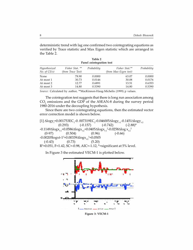
deterministic trend with lag one confirmed two cointegrating equations asverified by Trace statistic and Max Eigen statistic which are arranged inthe Table 2.
Table 2Panel cointegration test
Hypothesized Fisher Stat. ** Probability Fisher Stat.** ProbabilityNo. of CE(s) (from Trace Test) (from MaxEigen test)
None 78.90 0.0000 63.07 0.0000At most 1 30.73 0.0146 30.08 0.0176At most 2 12.77 0.6891 13.51 0.6353At most 3 14.80 0.5390 14.80 0.5390
Source: Calculated by author, **MacKinnonHaugMichelis (1999) p values.
The cointegration test suggests that there is long run association amongCO
2 emissions and the GDP of the ASEAN8 during the survey period
19802016 under the decoupling hypothesis.Since there are two cointegrating equations, then the estimated vector
error correction model is shown below.
[1]��logyt=0.001753EC
10. 007319EC
20.046005�logy
t10.1451�logy
t2
(0.293) (0.157) (0.742) (2.88)*0.1149�logx
t1+0.0586�logx
t2+0.0405�logx
t120.0258�log x
t22
(097) (0.504) (0.96) (0.66)0.00205logxt13+0.00339�logx
t23+0.0505
(0.43) (0.73) (5.20)R2=0.051, F=1.42, SC=0.98, AIC=1.12, *=significant at 5% level.
In Figure 3 the estimated VECM1 is plotted below.
Figure 3: VECM-1

Decoupling Co2 Emissions from GDP in Asean8: A Panel Data Analysis 9
VECM1 is a bad fit with low R2, F, and insignificant SC and AIC. Allcoefficients are insignificant except the coefficient of Älogy
t2. Yet the
coefficient of EC2 is negative but not significant which implies the
cointegrating equation tends to equilibrium with speed of adjustment 0.73% per year during 19802016.
[2] �logxt=0.00561EC
10.0446EC
2+0.02518�logy
t1+0.03508�logy
t2
(0.64) (0.65) (0.27) (0.47)+0.5608�logx
t10.2056�logx
t20.1269�logx
t120.00253�logx
t22
(3.24)* (1.21) (2.06) (0.04)+0.00949logx
t13+0.00172�logx
t23+0.06836
(1.36) (0.25) (4.59)*R2=0.066, F=1.86, SC=0.227, AIC=0.372, *=significant at 5% level.
VECM2 is also a bad fit with low R2, F, and insignificant SC and AIC.All coefficients are insignificant except the coefficient of �logx
t1. Yet the
coefficient of EC2 is negative but not significant which implies the
cointegrating equation tends to equilibrium with speed of adjustment 4.46% per year during 19802016.
In Figure 4 the estimated VECM2 is plotted below.
Figure 4: VECM-2
The estimated VECM3 is given below.[3] �logx
t2=0.040009EC
1+0. 251159EC
2+0. 4177�logy
t1+0. 2463�logy
t2
(0.68) (0.55) (0.691) (0.50)+0.6701�logx
t10.0923�logx
t20.27234�logx
t120.3935�logx
t22
(0.58) (1.08) (0.66) (1.006)

10 Debesh Bhowmik
+0.003398logxt1
3+0.0457�logxt2
3+0.533(0.73) (1.01) (5.36)*
R2=0.044, F=1.217, SC=3. 57, AIC=3.42, *=significant at 5% level.
VECM3 is not a good fit with low R2, F, and insignificant SC and AIC.All coefficients are insignificant. Yet, the coefficient of EC
1 is negative but
not significant which implies the cointegrating equation tends toequilibrium with speed of adjustment 4.0% per year during 19802016.
In Figure 5 the estimated VECM3 is plotted below.
Figure 5: VECM-3
The estimated VECM4 is shown below.[4]�logx
t3 = 0.0839EC
1+0.0474EC
2+1.58109�logy
t1+1.166�logy
t2
(0.22) (0.016) (0.40) (0.36)+3.0098�logx
t1+1.5038�logx
t22.1569�logx
t122.539�logx
t22
(0.40) (0.204) (0.80) (1.00)+0.3277logx
t13+0.2904�logx
t23+3.5351
(1.08) (0.99) (5.47)*R2=0.075, F=2.11, SC=7.31, AIC=7.16, *=significant at 5% level.
VECM4 is not a good fit with low R2, F, and insignificant SC andAIC. All coefficients are insignificant. Yet, the coefficient of EC
1 is
negative but not significant which implies the cointegrating equationtends to equilibrium with speed of adjustment 8.39% per year during19802016.

Decoupling Co2 Emissions from GDP in Asean8: A Panel Data Analysis 11
In Figure 6 the estimated VECM4 is plotted below.
Figure 6: VECM-4
Source: Plotted by author
Four pairs of cointegrating equations of estimated VECM can be foundfrom the system equations .
In the system equation of VECM1, the corresponding cointegratingequations are as follows:
[i] �logyt=0.001753logy
t14.543logx
t12+0.39715logx
t13+33.82
(0.293) (2.38)* (1.276)[ii] �logy
t=0.007319logx
t10.8101logx
t12+0.06732logx
t13+4.4217
(0.157) (3.33)* (1.69)
Cointegrating equationii has been approaching towards equilibriumwhich implies there is long run causality from logx
t1, logx
t12and log x
t13 to
��logyt although it is insignificant. The speed of adjustment is 0. 73% per
year and *=significant at 5% level.In the system equation of VECM2, the corresponding cointegrating
equations are as follows:
[iii] �logxt=0.0056logy
t14.543logx
t12+0.39715logx
t13+33.82
(0.64) (2.38)* (1.276)[iv] �logx
t=0.0446logx
t10.8101logx
t12+0.06732logx
t13+4.4217
(0.656) (3.33)* (1.69)

12 Debesh Bhowmik
Cointegrating equationiv has been approaching towards equilibriumwhich implies there is long run causality from log x
t1, log x
t12 and log
xt1
3 to ��logxt although it is insignificant. The speed of adjustment is 4. 46%
per year and *=significant at 5% level.In the system equation of VECM3 , the corresponding cointegrating
equations are as follows:
[v] �logxt2=0.0400logy
t14.543logx
t12+0.39715logx
t13+33.82
(0.686) (2.38)* (1.276)[vi] �logx
t2=0.2511logx
t10.8101logx
t12+0.06732logx
t13+4.4217
(0.552) (3.33)* (1.69)
Cointegrating equationv has been tending towards equilibrium whichimplies there is long run causality from log y
t1, log x
t12 and log
xt1
3 to ��log xt2 although it is insignificant. The speed of adjustment is 4.0%
per year and *=significant at 5% level.In the system equation of VECM4 , the corresponding cointegrating
equations are as follows:
[vii] �logxt3=0.0839logy
t14.543logx
t12 + 0.39715logx
t13 + 33.82
(0.221) (2.38)* (1.276)[viii] �logx
t3=0.0474logx
t10.8101logx
t12+0.06732logx
t13+4.4217
(0.016) (3.33)* (1.69)
Cointegrating equationvii has been moving towards equilibrium whichimplies there is long run causality from log y
t1, log x
t12 and log
xt1
3 to �log xt3 although it is insignificant. The speed of adjustment is 8. 39%
per year and *=significant at 5% level.The short run causalitieswere found from the Walt test and the
observations are as follows.[i] There are short run causalities from �log y
t1 and ��log y
t2 to �logy
t
because �2(2)=0. 0141 is rejected from the Wald Test where H0=no
causality where c(3)=c(4)=0.
[ii] There are short run causalities from �log xt1
and ��log xt2
to ��log xt
because �2(2)=0. 0051 is rejected from the Wald Test where H0=no
causality where c(16)=c(17)=0.
[iii] There are short run causalities from ��logxt1
2 and ��logxt2
2 to ��logxt
because �2(2) = 0. 098 is rejected from the Wald Test where H0=no
causality where c(18)=c(19)=0.
Their two cointegrating equations in terms of graph of cointegrationtest are shown in the Figure 7.

Decoupling Co2 Emissions from GDP in Asean8: A Panel Data Analysis 13
In general, the VECM is stable because there are 3 unit roots,two roots are less than one, one root is negative and six roots areimaginary under AR roots of characteristic polynomial. These are shownin Table 3.
Table 3Values of roots
Root Modulus
1.001425 1.001425
1.000000 1.000000
1.000000 1.000000
0.862635 0.862635
0.277945 0.353104i 0.449372
0.277945 + 0.353104i 0.449372
0.056787 0.413282i 0.417165
0.056787 + 0.413282i 0.417165
0.029794 0.390006i 0.391142
0.029794 + 0.390006i 0.391142
0.218469 0.218469
0.108898 0.108898
Source: Calculated by author
In the unit circle all roots lie inside or on the circle which proved thatVECM is stable and nonstationary.
All the variables in the VECM suffer from autocorrelation problem that’swhy the correlogram showed vertical bars are either sides which are shownin Figure 9.
Figure 7: Cointegration graph
Source: Plotted by author

14 Debesh Bhowmik
Figure 8: Unit circle
Source: Plotted by author
Figure 9: Autocorrelation
Source: Plotted by author
-.2
-.1
.0
.1
.2
1 2 3 4 5 6 7 8 9 10 11 12
Cor(LOG(Y),LOG(Y)(-i ))
-. 2
-.1
.0
.1
.2
1 2 3 4 5 6 7 8 9 10 11 12
Cor(LOG(Y),LOG(X)(-i))
-.2
-.1
.0
.1
.2
1 2 3 4 5 6 7 8 9 10 11 12
Cor(LOG(Y),LOG(X)̂ 2(-i))
-.2
-.1
.0
.1
.2
1 2 3 4 5 6 7 8 9 10 11 12
Cor(LOG(Y),LOG(X)^3(-i ))
-.2
-.1
.0
.1
.2
1 2 3 4 5 6 7 8 9 10 11 12
Cor(LOG(X),LOG(Y)(-i ))
-. 2
-.1
.0
.1
.2
1 2 3 4 5 6 7 8 9 10 11 12
Cor(LOG(X),LOG(X)(-i))
-.2
-.1
.0
.1
.2
1 2 3 4 5 6 7 8 9 10 11 12
Cor(LOG(X),LOG(X)̂ 2(-i))
-.2
-.1
.0
.1
.2
1 2 3 4 5 6 7 8 9 10 11 12
Cor(LOG(X),LOG(X)^3(-i ))
-.2
-.1
.0
.1
.2
1 2 3 4 5 6 7 8 9 10 11 12
Cor(LOG(X)̂ 2,LOG(Y)(-i ))
-. 2
-.1
.0
.1
.2
1 2 3 4 5 6 7 8 9 10 11 12
Cor(LOG(X)̂ 2,LOG(X)(-i))
-.2
-.1
.0
.1
.2
1 2 3 4 5 6 7 8 9 10 11 12
Cor(LOG(X)̂ 2,LOG(X)^2(-i ))
-.2
-.1
.0
.1
.2
1 2 3 4 5 6 7 8 9 10 11 12
Cor(LOG(X)̂ 2,LOG(X)̂ 3(-i))
-.2
-.1
.0
.1
.2
1 2 3 4 5 6 7 8 9 10 11 12
Cor(LOG(X)̂ 3,LOG(Y)(-i ))
-. 2
-.1
.0
.1
.2
1 2 3 4 5 6 7 8 9 10 11 12
Cor(LOG(X)̂ 3,LOG(X)(-i))
-.2
-.1
.0
.1
.2
1 2 3 4 5 6 7 8 9 10 11 12
Cor(LOG(X)̂ 3,LOG(X)^2(-i ))
-.2
-.1
.0
.1
.2
1 2 3 4 5 6 7 8 9 10 11 12
Cor(LOG(X)̂ 3,LOG(X)̂ 3(-i))
Autocorrelations with 2 Std.Err. Bounds

Decoupling Co2 Emissions from GDP in Asean8: A Panel Data Analysis 15
The VEC residual normality test of HansenDoornik(1994 ) residualcorrelation showed that the Chisquares values of skewness and kurtosisand the values of JarqueBera were not accepted for normality during 19802016 which is shown in the Table 4.
Table 4Normality test
Component Skewness Chisquare Degree of freedom Probability.
1 0.311402 4.433455 1 0.03522 2.748108 123.0982 1 0.00003 0.759953 22.30854 1 0.00004 1.093667 39.48967 1 0.0000
Joint 189.3298 4 0.0000Component Kurtosis Chisquare Degree of freedom Probability.
1 7.747851 108.2612 1 0.00002 22.92494 0.592656 1 0.44143 20.90326 521.8076 1 0.00004 22.66816 486.2992 1 0.0000
Joint 1116.961 4 0.0000Component JarqueBera Degree of freedom Probability.
1 112.6946 2 0.00002 123.6908 2 0.00003 544.1162 2 0.00004 525.7889 2 0.0000
Joint 1306.290 8 0.0000
Source: Calculated by author
The Impulse Response Functions assure that any external shocks fromthe independent variables on the emission do not move the system intothe equilibrium i. e. the functions diverge from the equilibrium which isshown in the Figure 10.
VI. LIMITATION AND THE FUTURE PROSPECT OF RESEARCH
Pollution is not simply a function of income but depends on manyfactors;such as the effectiveness of government regulations, thedevelopment of the economy, population level, energy price shock, literacy,income inequality, structural shifts in manufacturing, trade openness onenvironmental quality and other socioeconomic variables. Even,environmental impacts also fall with technological development.Sometimes, EKC may be N shaped. In this model, the inverted U shapedwould be more perfect if the observations are to be very large. The linkbetween Kaya identity to the EKC hypothesis and the decompositionanalysis in ASEAN8 are absent here although there is positive associationamong CO
2emission, GDP and carbon intensity which is highly significant

16 Debesh Bhowmik
at 5% level in ASEAN8 during 19802016 under fixed effect panel regressionmodel.
�y = 1077. 443+433. 9351�x + 15. 81398�(y/x)(1. 103) (8. 508)* (3. 448)*
R2=0. 313, F=3. 089*, DW=2. 36
Actual and estimated lines of Kaya equation in ASEAN8 have beenapproaching towards equilibrium point which is shown in Figure 11.
Moreover, the diagnostic test for coefficients of the estimated equationin confidence ellipse at 5% significant level is proved to be accepted whichis shown in Figure 12.
VII. POLICY RECOMMENDATIONS
The imposition of emission tax, carbon tax, a system of tradable emissionquota, a ceiling on total annual emissions level and increase in productionof renewable energy are recommended to reduce emissions level of ASEAN.More convergence of GDP are necessary among ASEAN regions whichcan accelerate emission reduction in the countries of the bloc in EKChypothesis.
- .04
.00
.04
.08
.12
.16
1 2 3 4 5 6 7 8 9 10
Response of LOG(Y) to LOG(Y)
-.04
.00
.04
.08
.12
.16
1 2 3 4 5 6 7 8 9 10
Response of LOG(Y) to LOG(X)
-.04
.00
.04
.08
.12
.16
1 2 3 4 5 6 7 8 9 10
Response of LOG(Y) to LOG(X)^2
-.04
.00
.04
.08
.12
.16
1 2 3 4 5 6 7 8 9 10
Response of LOG(Y) to LOG(X)^3
.0
.1
.2
1 2 3 4 5 6 7 8 9 10
Response of LOG(X) to LOG(Y)
.0
.1
.2
1 2 3 4 5 6 7 8 9 10
Response of LOG(X) to LOG(X)
.0
.1
.2
1 2 3 4 5 6 7 8 9 10
Response of LOG(X) to LOG(X)^2
.0
.1
.2
1 2 3 4 5 6 7 8 9 10
Response of LOG(X) to LOG(X)^3
0.0
0.4
0.8
1.2
1.6
1 2 3 4 5 6 7 8 9 10
Response of LOG(X)^2 to LOG(Y)
0.0
0.4
0.8
1.2
1.6
1 2 3 4 5 6 7 8 9 10
Response of LOG(X) 2̂ to LOG(X)
0.0
0.4
0.8
1.2
1.6
1 2 3 4 5 6 7 8 9 10
Response of LOG(X)^2 to LOG(X)̂ 2
0.0
0.4
0.8
1.2
1.6
1 2 3 4 5 6 7 8 9 10
Response of LOG(X)^2 to LOG(X)^3
0
2
4
6
8
1 2 3 4 5 6 7 8 9 10
Response of LOG(X)^3 to LOG(Y)
0
2
4
6
8
1 2 3 4 5 6 7 8 9 10
Response of LOG(X) 3̂ to LOG(X)
0
2
4
6
8
1 2 3 4 5 6 7 8 9 10
Response of LOG(X)^3 to LOG(X)̂ 2
0
2
4
6
8
1 2 3 4 5 6 7 8 9 10
Response of LOG(X)^3 to LOG(X)^3
Response to Cholesky One S.D. Innov ations
Figure 10: Impulse Response Functions
Source: Plotted by author

Decoupling Co2 Emissions from GDP in Asean8: A Panel Data Analysis 17
Figure 11: Estimated Kaya equationSource: Plotted by author
Figure 12: Diagnostic test for coefficients
Source: Plotted by author

18 Debesh Bhowmik
VIII. CONCLUSIONS
The paper concludes thatthere is no decoupling because the elasticity ispositive and greater than or equal to +1. 0 with respect to GDP, there isabsolute decoupling when the elasticity is zero or negative with respect tosquare of GDP, and there is relative decoupling with respect to the cube ofGDP during the survey period. All are significant at 5% level. Thus, it provesthe existence of inverted Ushaped Environment Kuznets Curve. Residualcross section dependence test confirmed that there is cross sectiondependence in the statistic of BreuschPagan LM (1979) and Pesaran CD(2015) which were rejected at null hypothesis of no crosssectiondependence (correlation) in residuals. The coefficient diagnostic testassured that the confidence ellipseis significant at 5% level. The cointegration test suggests that there is long run association among CO
2
emissions and the GDP of the ASEAN8 having two cointegratingequations given by Trace and Max Eigen statistic. From the VECM1of thesystem equation, cointegrating equation2has been approaching towardsequilibrium which implies there is long run causality from GDP of previousperiod, square of GDP of previous period, and cube of GDP of previousperiod to the change of CO
2 emission although it is not significant at 5%
level. The speed of adjustment is 0. 73% per year. The similar findings havebeen observed from other estimated VECM of the system equations. But,there is no short run causality from GDP to CO
2 emission in ASEAN8.
Besides, there are both short run and long run causalities from GDP, squareof GDP and cube of GDP of previous periods to GDP of the given period.In general, VECM is stable but nonstationary, nonnormal and seriallycorrelated.
References
Asante, Kwesi. (2016). Study on the Evidence of the Environmental Kuznets CurveHypothesis in Ghana, KOILAKAIST Scholarship programme.
Armeanu, Daniel et al. (2018). Exploring the link between environmental pollutionand economic growth in EU28 countries:Is there an Environmental Kuznets Curve?Plos One, 128.
Bhowmik, Debesh. (2018). Decoupling per capita CO2 emission from GDP per capita
in South Asia and Euro Area:Panel Data Analysis, Paper presented at Birla GlobalUniversity on 2324 November, Bhubaneshwar.
Breusch, T. S., & Pagan, A. R. (1979). A simple test for heteroscedasticity and randomcoefficient variation. Econometrica, 47(5), 12871287.
Finel, Nufar., & Tapio, Petri. (2012). Decoupling Transport CO2 from GDP. FinlandFutures Research Centre, University of Turku.
Fisher, R. A. (1932). Statistical Methods for Research Workers. Edinburg: Oliver & Boyd.12th Edition.

Decoupling Co2 Emissions from GDP in Asean8: A Panel Data Analysis 19
Grossman, G. M., & Krueger, A. B. (1991). Environmental impact of NorthAmericanFree Trade Agreements . Working Paper3914, NBER.
Grossman, G. M., & Krueger, A. B. (1995). Economic growth and the Environment.TheQuaterly Journal of Economics, 110(2), 353377.
Hansen, H., & Doornik, J. A. (1994). An omnibus test for univariate and multivariatenormality. Discussion Paper, Nuffield College, Oxford University.
Hausman, J. A. (1978). Specification Test in Econometrics. Econometrica, 46(6), 12511271.
Honma, S. (2014). Environmental and economic efficiencies in the AsiaPacific region.Journal of AsiaPacific Business, 15(2), 122135.
Johansen, S. (1988). Statistical Analysis of Cointegrating Vectors. Journal of EconomicDynamics and Control, 12, 231254.
Johansen. S. (1991). Estimation and Hypothesis Testing of Cointegration Vectors inGaussian Vector Autoregressive Models. Econometrica, 59(6), 15511580.
Joshua Sunday et al. (2017). Decoupling CO2 emission and economic growth in China:Is
there consistency in estimation results in analyzing Environmental Kuznets Curve?Journal of Cleaner Production.
Kaya, Y. (1990). Impact of carbon dioxide emissions on GDP growth:Interpretation ofproposed scenarios, www.wiki.nus.edu.sg
Kuznet, Simon. (1955). Economic growth and Income Inequality. American EconomicReview, 45, 128.
Li Nan et al. (2017). Energy structure, economic growth, and carbon emissions:Evidencefrom Shaanki Province of China (19902012). Forum Scientiae Oeconomic , 5(1), 7993.
Lise, W. et al. (2007). Energy consumption and GDP in Turkey:Is there a cointegrationrelationship? Energy Economics, 29(6), 116678.
Lu et al. (2007). Decomposition and decoupling effects of carbon dioxide emission fromhighway transportation in Taiwan, Germany, Japan and South Korea. Energy Policy,35, 32263235.
Marques, A. C., Fuinhas, J. A., & Leal, P. A. (2018). The Impact of economic growth onCO2 emissions in Australia:The Environment Kuznets Curve and decoupling index.Environment Science Pollution Research International, 25(27), 2728327296.
Pesaran, M. H. (2004). General Diagnostic test for cross section dependence in Panels.CESIFO, Working Paper, 1229, IZA Paper No1240.
Pesaran, M. H. (2015). Testing weak cross sectional dependence in large panel.Econometric Reviews, 34, 10881116.
Shafik, Nemat. (1994). Economic development and environment quality:An econometricanalysis. Oxford Economic Papers, 46, 757773.
Simon, J. L. (1996). The Ultimate Resource. Princeton: Princeton University Press.
Stern, David I. (1998). Progress on the environment Kuznets curve? Environment andDevelopment Economics, 3(2), 173196.
Sugiawam, Yogi., & Managi, Shunsuke. (2016). The Environmental Kuznets Curve inIndonesia:Exploring the potential of renewable energy. MPRA Paper No80839.

20 Debesh Bhowmik
Tapio, P. (2005). Towards a theory of decoupling in the EU and the case of road trafficin Finland between 1970 and 2001. Transport Policy, 35, 137151.
Uchiyama, Katsuhisa (2018). Environmental Kuznets Curve Hypothesis and CarbonDioxide Emissions, Springer.
Wald, Abraham (1943). Test of Statistical Hypothesis concerning several parameterswhen the number of observations is large. Transactions of American MathematicalSociety, 54, 42682.
Wang, Min Na. (2017). Investing the environment Kuznets Curve of Consumption fordeveloping and developed countries: A study of Albania and Sweden, Bachalor’sThesis, Aalto University.
Zhou, H. M. et al. (2016). The effect of FDI , economic growth and energy consumptionon carbon emission in ASEAN5: Evidence from panel quantile regression. EconomicModelling, 58, 237248.
Zhou, Yefan., Sirisrisakulchai, Jirakom., Liu, Jianxu., & Sriboonchitta, Songsak. (2018).The Impact of economic growth and energy consumption on carbon emissions:Evidence from panel quantile regression. Journal of Physics, Conference Series,Volume1053.