This document is downloaded from DR‑NTU (https://dr.ntu.edu.sg)Nanyang Technological University, Singapore.
Data‑driven product family design for additivemanufacturing
Lei, Ningrong
2016
Lei, N. (2016). Data‑driven product family design for additive manufacturing. Doctoralthesis, Nanyang Technological University, Singapore.
https://hdl.handle.net/10356/66496
https://doi.org/10.32657/10356/66496
Downloaded on 08 Mar 2022 14:23:03 SGT
DATA-DRIVEN PRODUCT FAMILY DESIGN
FOR
ADDITIVE MANUFACTURING
LEI, NINGRONG
School of Mechanical and Aerospace Engineering
A thesis submitted to the Nanyang Technological Universityin partial ful�llment of the requirement for the degree of
Doctor of Philosophy
2016

Acknowledgement
I would like to extend my appreciation to all of those who helped and contributed, in
one form or another, through my Doctor of Philosophy (PhD) research. My deep love
and gratitude go to my family who provide me their unconditional love, full support and
encouragement throughout all my life. The love, support, inspiration from my husband,
Oliver, helped me through the challenges of PhD study and make me a better person.
I would like to express my gratitude to my supervisor, Dr. Seung Ki Moon for
his support, advice, insights, and encouragement throughout of my PhD research. He
provided me many opportunities to advance my research and improve professional skills
through research collaboration, projects, and international conferences. I also would like
to thank Dr. Chun-Hsien Chen and Dr. Songlin Chen for their comments and suggestions
during our discussions on product development. Special thanks to Dr. Guijun Bi who
I collaborated on a joint research project between Singapore Institute of Manufacturing
Technology (SIMTech) and Nanyang Technological University (NTU).
Thanks to my colleagues, Samyeon, Xiling, Hyunwoong, Passarporn, and Yun En in
the Design Sciences Laboratory at NTU, Singapore. I cherish the discussions and time
we spent together.
I would like to thank Dr. David, W. Rosen from George W. Woodru� School of
Mechanical Engineering at Georgia Institute of Technology for inviting me as a visiting
scholar there. This opportunity provided great opportunity for me to bring the depth
and width to my research. During my brief stay, I am indebted to Jane and Chad for
I

their helpful discussions and for letting me use, modify and improve on their designs of
�nger pump family.
Finally, I would like to thank the School of Mechanical and Aerospace Engineer at
NTU for providing the scholarship to support my research.
II
Contents
1 Introduction 1
1.1 Research background . . . . . . . . . . . . . . . . . . . . . . . . . . . . . . 2
1.2 Research motivation . . . . . . . . . . . . . . . . . . . . . . . . . . . . . . 6
1.3 Research objectives and scope . . . . . . . . . . . . . . . . . . . . . . . . . 8
1.4 Overview of the thesis . . . . . . . . . . . . . . . . . . . . . . . . . . . . . 8
2 Literature review 11
2.1 Product family and product platform design tools and methods . . . . . . 12
2.2 Market segmentation and product positioning with data mining and ma-
chine learning techniques . . . . . . . . . . . . . . . . . . . . . . . . . . . . 18
2.3 Multi-objective decision support problems . . . . . . . . . . . . . . . . . . 22
2.4 Additive manufacturing facilitates customization . . . . . . . . . . . . . . 28
2.5 Summary and preview . . . . . . . . . . . . . . . . . . . . . . . . . . . . . 33
3 A data-driven product family design method for additive manufac-
turing 35
3.1 Overview and rationale . . . . . . . . . . . . . . . . . . . . . . . . . . . . . 35
3.2 The method: data-driven product family design for additive manufacturing 37
3.2.1 Step 1: data-driven market segmentation and product positioning . 39
3.2.2 Step 2: rede�ne customization for additive manufacturing . . . . . 42
III
3.2.3 Step 3: formulate a utility-based compromise decision support
problem . . . . . . . . . . . . . . . . . . . . . . . . . . . . . . . . . 44
3.2.4 Step 4: solve the decision support problem . . . . . . . . . . . . . . 46
3.3 Summary and preview . . . . . . . . . . . . . . . . . . . . . . . . . . . . . 47
4 A data-driven decision support system for market segmentation and
product positioning 49
4.1 Overview of the decision support system . . . . . . . . . . . . . . . . . . . 50
4.2 The construction of the decision support system . . . . . . . . . . . . . . . 52
4.2.1 Data preparation . . . . . . . . . . . . . . . . . . . . . . . . . . . . 54
4.2.2 Decision support with the DSSDB Explorer . . . . . . . . . . . . . 54
4.3 Market segmentation and product positioning of the automotive market . 62
4.3.1 Use case data . . . . . . . . . . . . . . . . . . . . . . . . . . . . . . 63
4.3.2 Use case testing . . . . . . . . . . . . . . . . . . . . . . . . . . . . . 64
4.3.3 Discussion . . . . . . . . . . . . . . . . . . . . . . . . . . . . . . . . 70
4.4 Summary and preview . . . . . . . . . . . . . . . . . . . . . . . . . . . . . 73
5 Data-driven decision support system design and evaluation 76
5.1 Overview of data-driven decision support system design problems . . . . . 77
5.2 Design and evaluation of the decision support system . . . . . . . . . . . . 79
5.2.1 Intrinsic dimensionality estimation . . . . . . . . . . . . . . . . . . 79
5.2.2 Dimensionality reduction . . . . . . . . . . . . . . . . . . . . . . . 83
5.2.3 Clustering . . . . . . . . . . . . . . . . . . . . . . . . . . . . . . . . 84
5.2.4 Performance evaluation . . . . . . . . . . . . . . . . . . . . . . . . 85
5.3 A robust decision support system for market segmentation and product
positioning . . . . . . . . . . . . . . . . . . . . . . . . . . . . . . . . . . . 87
5.3.1 An example: automobile market segmentation . . . . . . . . . . . . 87
5.3.2 Lessons learned . . . . . . . . . . . . . . . . . . . . . . . . . . . . . 90
IV
5.4 Summary and preview . . . . . . . . . . . . . . . . . . . . . . . . . . . . . 93
6 Product family design for additive manufacturing 95
6.1 Overview of in�uences of additive manufacturing to product family design 96
6.2 An additive manufacturing process model for product family design . . . . 98
6.2.1 Product family design . . . . . . . . . . . . . . . . . . . . . . . . . 98
6.2.2 Topology optimization . . . . . . . . . . . . . . . . . . . . . . . . . 100
6.2.3 Finite element analysis and cost analysis . . . . . . . . . . . . . . . 101
6.2.4 Customized product family . . . . . . . . . . . . . . . . . . . . . . 103
6.3 Designing a family of cantilever beams . . . . . . . . . . . . . . . . . . . . 103
6.3.1 Product family optimization . . . . . . . . . . . . . . . . . . . . . . 104
6.3.2 Finite element analysis and performance surfaces . . . . . . . . . . 106
6.3.3 Cost analysis . . . . . . . . . . . . . . . . . . . . . . . . . . . . . . 108
6.3.4 Customization of the cantilever beam product family . . . . . . . . 110
6.3.5 Beam fabrication and mechanical veri�cation . . . . . . . . . . . . 111
6.4 Summary and preview . . . . . . . . . . . . . . . . . . . . . . . . . . . . . 113
7 Data-driven product family design for additive manufacturing: design
of a �nger pump family 115
7.1 Overview of the dialysis pump design problem . . . . . . . . . . . . . . . . 116
7.2 The �nger pump family design . . . . . . . . . . . . . . . . . . . . . . . . 118
7.2.1 The �nger pump model description . . . . . . . . . . . . . . . . . . 118
7.2.2 Step 1: de�ne market segmentation . . . . . . . . . . . . . . . . . . 121
7.2.3 Step 2: optimize individual products for additive manufacturing . . 122
7.2.4 Step 3: formulation of the utility-based product family design prob-
lem . . . . . . . . . . . . . . . . . . . . . . . . . . . . . . . . . . . . 127
7.2.5 Step 4: Solve the optimization problem to de�ne the product family130
7.3 Comparison to product platform constructal theory method results . . . . 131
V
7.4 Summary . . . . . . . . . . . . . . . . . . . . . . . . . . . . . . . . . . . . 134
8 Closure: achievements and recommendations 136
8.1 Research summary . . . . . . . . . . . . . . . . . . . . . . . . . . . . . . . 136
8.2 Research contributions . . . . . . . . . . . . . . . . . . . . . . . . . . . . . 138
8.3 Limitations . . . . . . . . . . . . . . . . . . . . . . . . . . . . . . . . . . . 140
8.4 Recommendations and future work . . . . . . . . . . . . . . . . . . . . . . 142
8.5 Concluding remarks . . . . . . . . . . . . . . . . . . . . . . . . . . . . . . 143
Bibliography 145
A 168
A.1 Acronyms . . . . . . . . . . . . . . . . . . . . . . . . . . . . . . . . . . . . 168
A.2 Matlab code . . . . . . . . . . . . . . . . . . . . . . . . . . . . . . . . . . . 172
VI
Summary
Platform based product family design is a promising approach to meet diverse Customer
Needs (CNs) and achieve organizational objectives. We have dedicated this work to
improve product family design by incorporating advanced information and new manu-
facturing technologies. Our e�ort resulted in a data-driven product family design for
Additive Manufacturing (AM) method. The proposed data-driven approach used Data
Mining (DM) to extract meaningful information from market data. The extracted in-
formation was interpreted by advanced machine learning algorithms to form a Decision
Support System (DSS), that helps designers make informed decisions for market seg-
mentation and product positioning. Based on the identi�ed market segments, an AM
process model for product family design was developed to o�er a�ordable customization
for each targeted market segment. Finally, a Utility-Based Compromise Decision Support
Problem (u-cDSP) was formulated to serve as a mathematical framework for modeling
a multi-objective product family design problem. The thesis highlights data-driven de-
cision making and the opportunities for AM based product family design to operate
in a much broader design space that is free from constraints which arise in traditional
product family designs from �nding a compromise between commonality and product
performances.
The data-driven product family design for AMmethod was tested and veri�ed through
three distinct case studies. The �rst case study focused on the design of a DSS for mar-
ket segmentation and product positioning based on US automotive market data. The
VII
proposed DSS automates market segmentation and product positioning and provides a
framework for the construction of a robust DSS. In the second case study, we used the
proposed method to design a product family of cantilever beams. We found that our
process model re�ects the ability of AM to produce arbitrarily complex structures with
virtually no tooling e�ort, and it makes these powerful properties available to practition-
ers working in the �eld of product family design. The �nal case study centered on the
design of a dialysis �nger pump family. The proposed method translates the bene�ts of
AM into improved customization and cost reduction without compromising individual
product performances.
We created new knowledge in the product family design area by describing the theo-
retical and empirical validation process of the data-driven product family design for AM
method. The main result of this research is a systematic framework which seamlessly
integrates AM technologies into product family design to facilitate improved customiza-
tion. The primary contribution of the framework is a data-driven DSS that advances
market segmentation and product positioning. It is expected that the proposed method
will rede�ne how we think about customization in product family design.
VIII

Chapter 1
Introduction
First, the taking in of scattered particulars under
one Idea, so that everyone understands what is
being talked about ... Second, the separation of the
Idea into parts, by dividing it at the joints, as
nature directs, not breaking any limb in half as a
bad carver might.
Plato, Phaedrus, 265 BC
This thesis proposes a data-driven product family design for Additive Manufacturing
(AM) method that helps companies meet increasing customization requirements. This
chapter presents carefully selected material on platform based product family design and
thereby it provides the background of our research work. Section 1.2 postulates three
research questions which sparked the research on data-driven product family design for
AM. Section 1.3 presents the research objectives, scope and contributions for the work.
Finally, Section 1.4 introduces the thesis overview.
1
1.1 Research background
We are living in the age of the �buyer's market� where the producer of goods must satisfy
individual customer requirements [1]. One way to meet the individual requirements is
the mass customization strategy. This strategy creates competitive market places, which
require manufacturers to introduce an increasing number of products with a shorter life
span at a lower cost [2]. Therefore, producers are continuously thriving to �nd new ways
for reducing the production cost, while still o�ering attractive products [3].
The product family paradigm has been proposed to address the challenges of designing
products for mass customization in order to meet diverse Customer Needs (CNs). The
term product family is frequently de�ned in the literature as a set of similar products
that are derived from a common platform and yet possess speci�c features/functionality
to meet particular customer requirements [4, 5, 6]. A member of a product family is
called product variant [4]. Each product variant possesses characteristics in response
to unique CNs. The product family paradigm introduces product proliferation while
taking advantage of mass production e�ciency [7]. Many companies invest in product
family development practices in order to provide su�cient variety to the market while
maintaining the economies of scale and scope within their manufacturing capabilities
[8]. The underlying focus of product family optimization is to design a group of related
products, which are built around a common functional system architecture known as
platform [4, 9]. Product platforms are commonly characterized by two types: modular
platforms and scalable platforms [10]. A modular platform is used to create variants
through the con�guration of existing modules [4, 11]. While a scalable platform facilitates
the di�erentiation of variants, that possess the same function, with varying capacities
[10].
Well-known examples of platform based product families include: Black and Decker©
power tools, HP© printers, IBM©, and Microsoft© Operation Systems [4]. Many in-
2

dustries have acknowledged the competitive advantages of product family and platform
approaches [12]. Product families are successful in the market place, because they ex-
ploit commonality between the family of products and thereby they o�er a competitive
advantage for companies. However, too much commonality (i.e. not enough diversity)
within a product family can lead to a lack of product distinctiveness and a compromise in
product performance. Consequently, there is an inherent trade-o� between commonality
and diversity within any product family [13, 14]. Conventional product family opti-
mization focuses on exploiting the commonality between individual products [15]. The
fundamental assumption is that common components are less cost intensive than dis-
tinctive ones. Hence, harvesting the bene�ts of product family design means to identify
features and functions that can be shared amongst products. However, product family
design compromises on which CNs are satis�ed. The compromise implies that some CNs
are not satis�ed. As a consequence companies struggle to realize the full potential of a
market. To rectify the shortcoming means to improve mass customization in order to
serve customers better and to achieve commercial success.
The main objective of the platform based product family design is to provide cost
e�ective product variety [9]. The objective is achieved by increasing the commonality
across multiple products and di�erentiating each product in the family by satisfying
individually targeted CNs. Before we can e�ectively meet diverse CNs, we have to
understand market segmentation, because the market segmentation strategy structures
the customer demands. To be speci�c, market segmentation divides the market into
customer clusters with similar needs or characteristics [16].
Meyer and Lehnerd developed a market segmentation grid, as shown in Figure 1.1.
It conceptualizes product platforms across di�erent market segments [4]. In the market
segmentation grid, major market segments, that are serviced by a company's products,
are listed horizontally. The vertical axis re�ects di�erent price and performance tiers
within each market segment. The market segmentation grid provides a useful attention
3
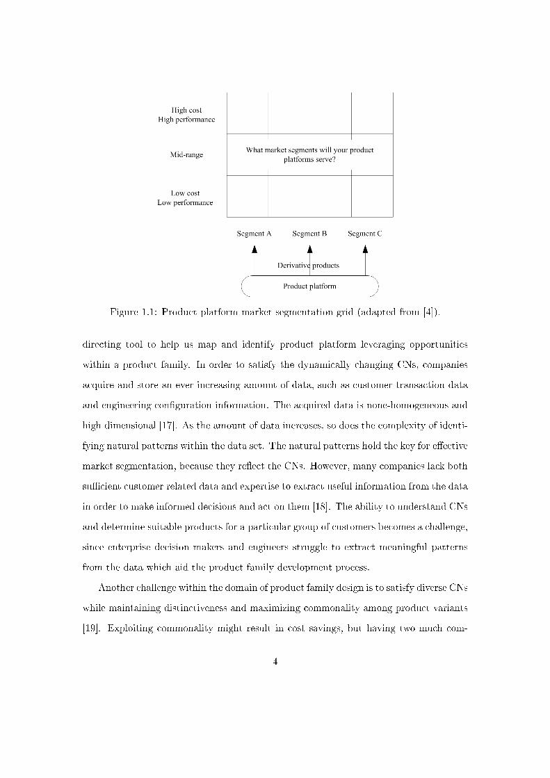
Figure 1.1: Product platform market segmentation grid (adapted from [4]).
directing tool to help us map and identify product platform leveraging opportunities
within a product family. In order to satisfy the dynamically changing CNs, companies
acquire and store an ever increasing amount of data, such as customer transaction data
and engineering con�guration information. The acquired data is none-homogeneous and
high dimensional [17]. As the amount of data increases, so does the complexity of identi-
fying natural patterns within the data set. The natural patterns hold the key for e�ective
market segmentation, because they re�ect the CNs. However, many companies lack both
su�cient customer related data and expertise to extract useful information from the data
in order to make informed decisions and act on them [18]. The ability to understand CNs
and determine suitable products for a particular group of customers becomes a challenge,
since enterprise decision makers and engineers struggle to extract meaningful patterns
from the data which aid the product family development process.
Another challenge within the domain of product family design is to satisfy diverse CNs
while maintaining distinctiveness and maximizing commonality among product variants
[19]. Exploiting commonality might result in cost savings, but having two much com-
4
monality in the product family may make some low-end products over-designed and some
high-end products under-designed. As a result, there is a danger of losing market share
in high-end market niches or wasting capital investment in low-end niches [20]. Further-
more, in a large product family, more compromises/trade-o�s are required, which cause
a degradation of individual product performances. When the product variants show too
many similar features and fail to be distinct from each other, a company might lose
the unique brand identity. As a consequence, the reduced brand identity might trigger
a loss of market share to the competition. Therefore, o�ering a�ordable customization
is the foremost challenge that enterprises face when they follow the product family de-
sign paradigm. The power of a company to o�er improved mass customization depends
on a good understanding of CNs and on the manufacturing capabilities. To translate
CNs data into tangible design decisions requires advanced information technology. Sim-
ilarly, the realization of the improved mass customization demands new and advanced
manufacturing technologies.
Innovations in manufacturing technology are likely to bring numerous competitive
advantages, such as low costs, superior quality, shorter delivery cycles, low inventories,
shorter and new product development cycles [21]. AM is such a technological innovation
which holds the promise to generate competitive advantages. The new technology can
be de�ned as �the process of joining materials to make objects from 3D model data,
usually layer upon layer, as opposed to subtractive manufacturing methodologies, such
as traditional machining� [22]. The competitive advantages arise from the fact that AM
technologies, unlike material removal processes, facilitate free-form fabrication of geo-
metrically complex parts without special �xtures and expensive tooling. Due to these
positive properties, AM has the potential to shorten the lead time signi�cantly and pro-
duce customized parts cost-e�ectively. However, a prerequisite to realize the competitive
advantages is a design methodology which unlocks the potential of AM.
We have dedicated this work to incorporate advanced information and new man-
5
ufacturing technology into product family design. This e�ort resulted a data-driven
product family design for AM method. The proposed data-driven approach used Data
Mining (DM) to extract meaningful information from market data. The extracted in-
formation was interpreted by advanced machine learning algorithms to form a Decision
Support System (DSS), that helps designers make informed decisions for market segmen-
tation and product positioning. Based on the identi�ed market segments, an AM process
model for product family design was developed to o�er a�ordable customization for each
targeted market segment. Finally, a Utility-Based Compromise Decision Support Prob-
lem (u-cDSP) was formulated to serve as a mathematical framework for modeling the
multi-objective product family design problem.
The proposed method is expressed in the research questions and hypotheses in the
next section.
1.2 Research motivation
The motivation of our research comes from the new challenges for product family de-
sign in the global competitive �buyer's market". The increasing demand for product
customization and the increasing capability to realize customization in a cost e�ective
way force companies to rethink their product family design strategies. The use of new
information and manufacturing technologies is not an option, it is a must for companies'
survival and pro�tability. As a consequence, there is a need for new design methodolo-
gies that incorporate advanced information and manufacturing technologies into product
family design.
After having established a powerful need for updated design methodologies, which
incorporate new technologies, as a key driver of the research work, we have to re�ne this
need into three major research questions.
6
Research question 1: How to enable more agile and more accurate decision-
making for market segmentation and product positioning?
Research question 2: How to incorporate AM into product family design
processes in order to facilitate customization in targeted market segments?
Research question 3: How to mathematically model and support product
platform decisions that involve multiple objectives?
The main hypothesis is that the data-driven product family design for AM method
has the ability to answer these research questions. The proposed method was developed
for the design of scalable product families. A scalable product family adjusts the platform
by changing values of dimensions or other parameters such that the resulting components
address speci�c CNs. For example, through scaling of a common set of design variables,
the product family can satisfy a wide variety of customer requirements without or with
minimum compromise in individual product quality and performances.
To address each research question in greater detail, the following one-to-one corre-
sponding sub-hypotheses are stated:
Sub-hypothesis 1: A DSS that employs advanced DM and machine learning
techniques can be developed to help designers identify market segmentation and
predict product positioning.
Sub-hypothesis 2: An AM process model for product family design can be
developed to incorporate AM into product family design process in order to
facilitate improved customization in target market segments.
Sub-hypothesis 3: A utility-based compromise Decision Support Problem
(DSP) can be formulated to model multiple objectives product family design
problem.
The sub-hypotheses are outlined here to provide context for the literature review in
the next chapter. Furthermore, they structure and guide the development of the proposed
method. The next section presents research objectives and research scope.
7

1.3 Research objectives and scope
The principal goal of the research work, presented in this thesis, is to develop a data-
driven product family design for AM method. The proposed method incorporates ad-
vanced DM and machine learning techniques, as well as AM into product family design.
We aim to provide a new product family design method that o�er improved customization
in a cost e�ective way. Keeping the primary research as a focus, the following detailed
objectives are investigated:
� Develop a robust DSS to automate and objectify market segmentation and product
positioning processes.
� Rede�ne the product family design process to accommodate AM for improved cus-
tomization.
� Analyze the manufacturing cost for Selective Laser Sintering (SLS) based product
family designs.
� Formulate and solve a u-cDSP for multi-objective product family optimization
problems.
Two main aspects of our method are: (1) objective decision making by using DM and
machine learning techniques for market segmentation and product positioning based on
market data; (2) Incorporating AM technologies into product family design to provide
improved customization.
1.4 Overview of the thesis
An overview of the thesis chapters is shown in Figure 1.2. As seen in the most left
column, there are four parts of the thesis structure, including problem identi�cation,
method, testing, and closure. The �ow chart column shows the relationship and logical
8
�ow of di�erent chapters. The relevance column brie�y introduces the main contents of
each chapter and its role in the thesis.
Having introduced the research background, motivation and objectives in this chapter,
the next chapter reviews the related state-of-the-art research, elucidating the research
gaps and opportunities in product family design. Four research areas are reviewed: (1)
product family design methods and tools (2) DM and machine learning techniques and
their roles in product family design, (3) multi-objective decision support problems, and
(4) AM technologies and their in�uence on mass customization.
The proposed data-driven product family design for AM method is illustrated in
Chapter 3. Chapter 4 introduces and veri�es the data-driven DSS for market segmen-
tation and product positioning. Chapter 5 augments the previous developed DSS and
develops a framework on how to construct a robust DSS for market segmentation and
product positioning. Chapter 6 demonstrates implementation of AM process model for
product family design. Chapter 7 fully implements the proposed data-driven product
family design for AM method on designing a family of �nger pumps. In each chapter, a
speci�c problem is identi�ed, the steps of the proposed method are performed, and the
rami�cations of the results are discussed.
Chapter 8 is the �nal chapter and it contains a summary of the thesis. Section 8.2
restates the research hypotheses and emphasizes research contributions. Limitations of
the research work and possible directions of future work are discussed in Sections 8.3 and
8.4 respectively. Final remarks are drawn in Section 8.5.
9
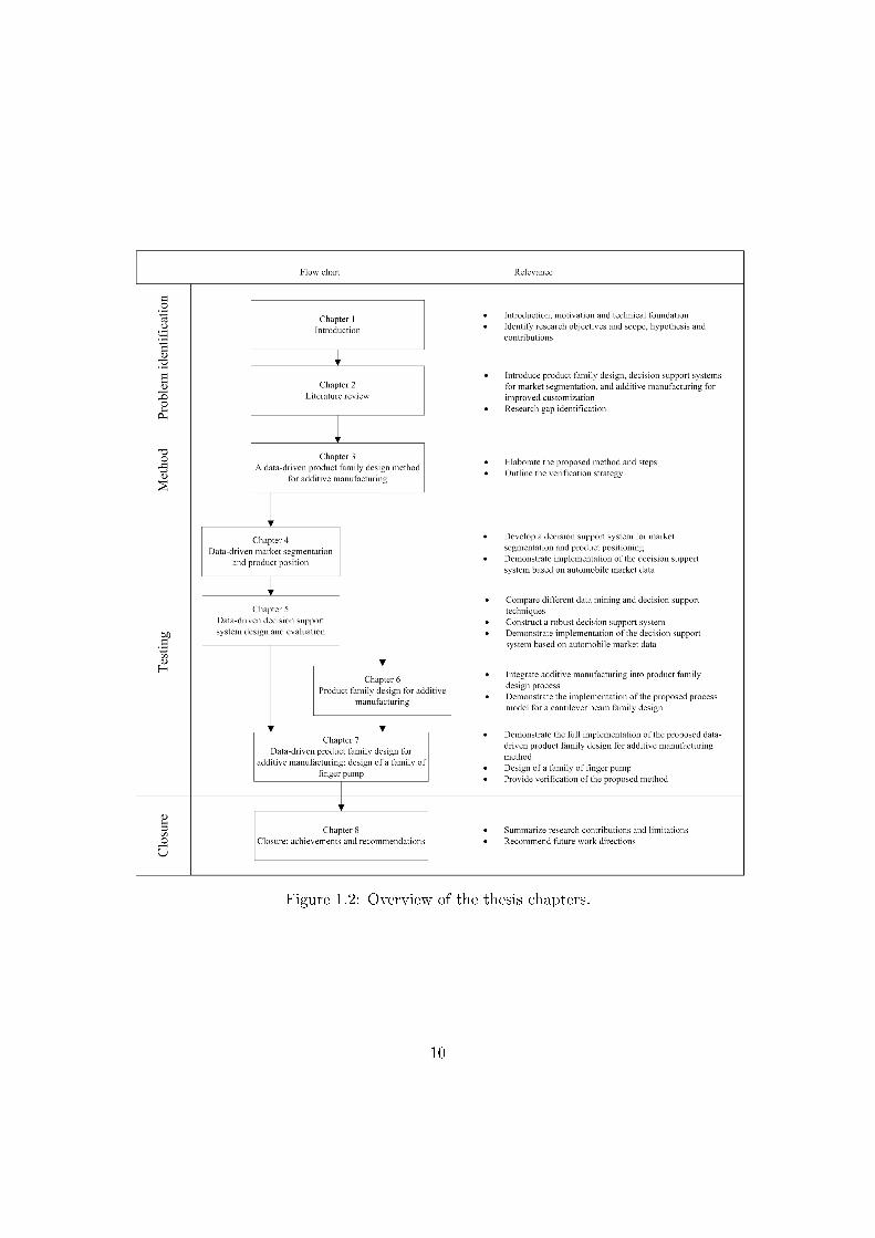
Figure 1.2: Overview of the thesis chapters.
10
Chapter 2
Literature review
In competitive markets, companies have to meet Customer Needs (CNs) in order to be
commercially successful. The problems on how to meet the CNs are not new. There
is a whole ecosystem, complete with research niches, of literature that aims to pro-
vide elegant solutions that address CNs in a most economic way. In this chapter, we
embark on the di�cult task of selecting and indeed justifying a manageable subset of
the problems, the solutions of which help companies provide improved and a�ordable
customization. The selection process starts by reviewing the argument that led to the
postulation of product family design methodologies. Based on the literature review, we
share the insight that product family design is greatly in�uenced by information and
manufacturing technologies. As a direct consequence of the realization, we investigated
new enabling technologies for product customization. Having intensely studied the me-
chanics of product family design and their intricate relationship with technologies, we
came to the conclusion that there is a need for integrating advanced data-driven infor-
mation technology and Additive Manufacturing (AM) into product family design. As
such, that is important work, because of the socio-economic interest in improving mass
customization.
Section 2.1 reviews and discusses the platform based product family design as one
11

method to optimize the product creation process. Increasing customer requirements and
changing socio-economic climate drive the complexity of product family design. To man-
age the increasing complexity, more and more designers employ Data Mining (DM) and
machine learning tools. Section 2.2 gives an overview of market segmentation and prod-
uct positioning methods with DM and machine learning techniques. Section 2.3 reviews
multi-objective product family design decision problems. Both the design itself and de-
sign strategies are not static, they have to adapt to changing CNs and new technologies.
Section 2.4 states how design methodologies need to change in order to facilitate new
technologies, such as AM. Each of these product family design approaches is critically
reviewed. Strengths, weaknesses and accepted application domains are discussed. Taken
together, the literature review provides the necessary constructs for the development of
the data-driven product family design for AM method as outlined in Chapter 3.
2.1 Product family and product platform design tools and methods
Platform based product family development has received much attention in both academia
and industries alike over last decades [19]. The reason for the wide spread interest comes
from the fact that this design strategy is seen as an economic way to achieve mass cus-
tomization. Conceptually, platform based product development unfolds as a logical and
organized method for generating a family of products [23]. The product platform provides
a generic umbrella to capture and utilize commonality, within which each new product
is instantiated and extended in order to anchor future designs to a common product line
structure.
The common product line structure is achieved by either modularization or scaling
the design parameters. Hence, platform based product families can be categorized into
modular product families and scalable product families [24].
� Modular product families: product family members are instantiated by adding,
12
substituting, and/or removing one or more functional modules from the product
platform [25, 26]. Modular platforms allow designers to create functionally di�erent
product variants.
� Scalable product families: scaling variables are used to �stretch� or �shrink� the
product platform in one or more dimensions to obtain di�erent product variants
[10]. Scalable platforms allow a designer to create functionally identical products
with di�erent capacities.
Modularization achieves cost savings by (a) harvesting the economies of scale for
modules that can be used across product families, (b) complexity reduction through-
out manufacturing and assembly processes, and (c) inventory reduction through risk
pooling and postponement [27]. Kreng and Lee synthesized modular design goals in
the literature into 14 module drivers: carryover, technology evolution, planned product
changes, standardization of common modules, product variety, customization, �exibil-
ity of use, product development, product development management, styling, purchasing
modularity components, manufacturability re�nement and quality assurance, quick ser-
vice and maintenance, product upgrading, recycling, reuse, and disposal [28]. These
module drivers were linked to di�erent company functions, such as product development
and design, production, after sales, etc. Various approaches have been developed to es-
tablish mathematical models for modularity and commonality. For example, Fujita and
Yoshida developed an algorithm that simultaneously optimizes both module attributes
and modular combinations [29]. In their model, modules are either independent, similar,
or common. Huang and Kusiak used a modular matrix to identify the number of modules
and the number of di�erentiation components, both values were selected such that they
satisfy varieties [30]. Ye et al. used a matrix-based design tool which supports clustering
product attributes into common, variable, and unique modules [31]. A detailed review
on metrics for modularity was done by Gershenson et al. [32]. As the amount of relevant
13

data and the product family design complexity increase, the design community faces
the challenge of �nding meaningful information to support design processes. Therefore,
the community turns to advanced information technologies in order to �nd solutions
for the eminent data overload. Some of the most promising techniques are information
extraction and decision support algorithms. Hence, these methods have been used to
extract meaningful information from modular design data. There are several methods
for grouping or distinguishing modules. For example, association rules and fuzzy cluster-
ing [33], mathematical programming [34], Genetic Algorithm (GA) [35], Particle Swarm
Optimization (PSO) [36]. This concludes our brief review of modular product family
design, the reader can refer to Jose and Tollenaere [37] and Joines and Culberth [38] for
a general view of modular methodologies.
Scalable product family design involves two basic tasks [19]. The �rst task is platform
selection � to determine which design parameters take common values. The second task is
design variable identi�cation � to determine the optimal values of common and distinctive
variables by satisfying performance and economic requirements. Several methods haven
been developed to design scalable platforms. Dai and Scott proposed the sensitivity anal-
ysis and cluster analysis based design method to improve both e�ciency and e�ectiveness
of a scalable product family design [20]. Nayak et al. proposed a variation-based plat-
form design methodology that aims to satisfy a range of performance requirements using
the smallest variation of product variants designs [39]. Simpson et al. introduced a prod-
uct platform concept exploration method called Product Platform Concept Exploration
Method (PPCEM) [19]. The corner stone of their method is a concept which minimizes
the sensitivity of performance variations in scaling factors. The PPCEM begins with
a market segmentation grid which is used to identify potential product family devel-
opment strategies. Subsequently, the product family design variables and performance
parameters are identi�ed. Next, product platform speci�cations are aggregated. The ag-
gregation step includes formulating an appropriate multi-objective model of the product
14
platform, in the form of a Compromise Decision Support Problem (cDSP). Finally, a
product platform, that best satis�es the overall design requirements, is obtained. Based
on a principle similar to PPCEM, the product variety trade-o� evaluation method was
presented by Simpson, et al [13]. The method is used to assess appropriate product family
trade-o�s using commonality and performance indices. In each of these approaches, the
set of scale factors and the common platform parameters are pre-selected. The method
we propose is based on similar assumptions.
Meyer and Lehnerd developed a three-level method for the design of a scalable
platform-based product family [4]. Figure 2.1 gives a graphical representation of the
design method. The method is structured into common building blocks, product plat-
forms, and market segmentation:
1. The common building blocks include consumer insights, product technologies, man-
ufacturing process, and organizational capabilities which are the basis for develop-
ing a product platform.
2. Product platforms constitute the basis for con�guring product variants. The vari-
ants, together with platforms, form a product family.
3. The market segmentation process identi�es a market segmentation grid. Each
market segment represents di�erent CNs. Each product variant addresses unique
customer requirements with its functionalities.
In the process of platform based product family planning and development, the mar-
ket segmentation grid, as shown in the market segmentation level of Figure 2.1, can
be used by companies to segment their markets and help in de�ning a clear product
platform strategy. The major market segments, serviced by a company's products, are
listed horizontally in the grid. The vertical axis re�ects di�erent tiers of price and per-
formance within each market segment. According to Meyer and Lehnerd, there are three
di�erent platform leveraging strategies within the market segmentation grid: horizontal
15
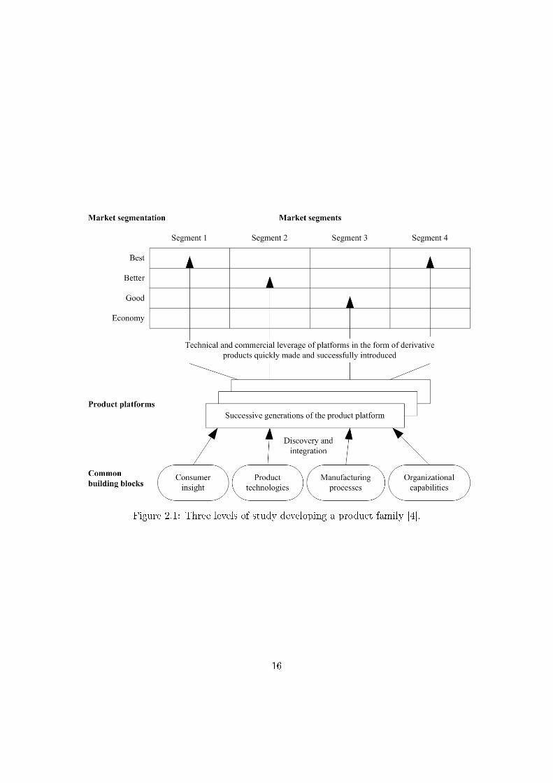
Figure 2.1: Three levels of study developing a product family [4].
16
leveraging, vertical leveraging, and the so called beachhead approach, which combines the
�rst two methods [4]. All three leveraging strategies enable a more e�cient and e�ec-
tive product family development. With all that research in the background, Simpson
et al. concluded that horizontal leveraging strategies always take advantage of modular
platforms, in contrast scale-based platform design can be used for vertical leveraging
strategies [13]. The methods and tools that haven been developed to identify market
segmentation is elaborated in the next section.
To help in designing and assessing a product platform, the degree of commonality be-
tween product variants, within a product family, is often used. Many commonality indices
have been developed based on di�erent parameters, such as number of common compo-
nents and their connections, costs, etc. These indices include: Degree of Commonality
Index (DCI), Commonality Index (CI), Generational Variety Index (GVI), Commonality
versus Diversity Index (CDI) [40, 41]. Common knowledge in the product family design
community is that products, which share more parts and modules within a product fam-
ily, achieve greater inventory reductions, exhibit less variability, improve standardization,
and shorten development and lead time, because more parts are reused and fewer new
parts have to be designed [42]. Simpson et al. developed a product variety trade-o�
evaluation method to help designers resolve the choice between platform commonality
and individual product performance within a product family [13]. The goal was achieved
through the use of two indices: the Non-Commonality Index (NCI) and the Performance
Deviation Index (PDI). Simpson et al. gave a comprehensive list and review of existing
commonality indices [19]. Thevenot et al. provided an extensive comparison between
many of these commonality indices [43].
Common to all the research discussed above is the realization that a successful prod-
uct platform must balance performance and commonality of individual products in the
family. The fundamental assumption is that common components are less cost intensive
than distinctive ones. Hence, harvesting the bene�ts of product family design means to
17
identify features and functions that can be shared among products. However, product
family design compromises on which CNs are satis�ed. Performance and commonality
are two con�icting objectives, a shared platform for all products in the family means to
establish an agreement which resolves the con�ict. The way in which the agreement is
reached depends also on the product variety induced manufacturing complexity, because
manufacturing complexity is a signi�cant cost factor and sometimes there are hard techni-
cal limitations [44]. Therefore, o�ering product variety without compromising individual
performance and realizing product variants in a cost e�ective manner are challenging
tasks that have to be addressed.
2.2 Market segmentation and product positioning with data mining and
machine learning techniques
Since the early 1960s, market segmentation is widely considered to be a key marketing
concept and a signi�cant amount of marketing research literature focused on this topic
[16]. The literature is concerned with the fact that a �rm must continuously reposition
and redesign its existing products or introduce new products to speci�c market segments
in order to maintain and enhance the level of pro�tability in an increasingly competi-
tive and transparent market place [45]. Decisions on market segmentation and product
positioning are crucial for companies to meet diverse CNs and achieve its goals. A com-
pany has to establish its market and subsequently subdivide the market so that it can
address the needs, posed by a particular market segment, with speci�c products. De-
spite the acknowledged importance of market segmentation for business practice, most
of the relevant literature is conceptual or normative in nature, dealing with how market
segmentation should be conducted [46, 47], rather than with how market segmentation
is actually performed in practice.
With the advent of cheap data storage and fast computers, the amount of engineering
18
data generated during design and development accumulates beyond the ability of human
beings to re�ne the data into knowledge or information. Yet, in the current volatile mar-
kets, accessing and distilling valuable knowledge, hidden in the vast amount of data, is
crucial [48]. Over the last few decades, DM and machine learning techniques for intelli-
gent analysis of large data volumes have been incorporated in the product design process
in order to improve and optimize engineering design and manufacturing process decisions
[49]. To keep their competitiveness, commercial organizations continuously monitor their
target market segments by gathering data from both consumers and competitors [50].
The resulting data is analyzed to form the basis for market segmentation and product po-
sitioning. The analysis quality de�nes the validity of both processes. As a consequence,
there is an urgent need to �nd and apply e�cient methods for extracting information
from the data.
In the context of product development, DM and machine learning are emerging ar-
eas of research that have the potential to signi�cantly impact on engineering design and
manufacturing e�orts [51, 52, 53]. Westphal and Blaxton identi�ed four functions of
DM: classi�cation, estimation, segmentation and description [54]. Classi�cation involves
assigning labels to previously unseen data records based on the knowledge extracted
from historical data. Estimation is the task of �ling in missing values in the �elds of an
incoming record as a function of �elds in other records. Segmentation (also called cluster-
ing) divides a population into smaller subpopulations with similar behavior. Clustering
methods maximize homogeneity within a group and maximize heterogeneity between the
groups. A description task focuses on explaining the relationships among the data.
A variety of DM and machine learning algorithms have been proposed to automate
or at least to support market segmentation and product positioning [55, 15]. Market
basket analysis (also known as Association Rule Mining (ARM)) is widely used to dis-
cover customer purchasing patterns by extracting associations or co-occurrences from
transactional databases [56]. Agard and Kusiak utilized DM, clustering techniques and
19
ARM to analyze the functional requirements in a new product development process and
thereby solve the customer segmentation problem [57]. Later works by Kusiak illustrated
the bene�ts of DM in a wide range of diversi�ed industries, such as biotechnology, en-
ergy, pharmaceutical, etc [51]. Yu and Wang proposed a genetic algorithm-based ARM
approach to capturing CNs and de�ning product speci�cation [58]. Chen et al. used
the machine learning method of Self-Organizing Map (SOM) to transfer customer re-
quirements into a speci�c product concept by considering a�ective factors from both
customers and designers [59]. Kuo et al. introduced a two-stage method that combined
SOM with the K-means algorithms [60]. Initially, SOM determined the number of clus-
ters and the starting point. Subsequently, the K-means method was used to �nd the
�nal solution. Tsai and Chiu embedded GA into a purchase-based segmentation algo-
rithm to identify market segmentation, based on product speci�c variables, such as the
purchased items and associated monetary expenses from transactional customer histories
[61]. Han et al. presented an market segmentation model using weighted fuzzy K-means
to support category management in convenience store chains [62]. Using three examples,
including retail sales forecasting, direct marketing and target marketing, Venugopal and
Baets demonstrated the capability of Arti�cial Neural Networks (ANNs) in marketing
management [63].
The successful development of DM-based knowledge discovery is a key issue to achieve
objective decision support for marketing research problem-solving [64]. Intelligent DM
and machine learning techniques can be used to extract nontrivial and potentially useful
patterns and information from otherwise incomprehensible data sets. These techniques
provide explicit information that has a human readable form and they can be used to
solve classi�cation or forecasting problems. Decisions, based upon the extracted patterns,
will be more reliable [64]. Plank observed that management decisions were a�ected by
the availability and use of market data [65]. However, many companies lack both data
and expertise to harvest useful information which helps them make informed decisions
20

and act on them [18]. Therefore, making market data directly accessible to decision
makers and providing decision support are essential for the success of a company [66].
The access must be as barrier free as possible and the decision support must be as reliable
as possible to ensure usability and to create a positive impact on management decisions,
targeting speci�c market segments and product o�erings.
Intelligent algorithms and advanced information technology have made cluster-based
marketing research more relevant. However, from the literature review, we discovered
that most researchers selected the methods and techniques without a coherent strategy on
an ad-hoc basis. Fewer e�orts were devoted into the discussion of applicability and �tness
of the existing methods [67]. K-means is one of the most commonly used algorithms in
market research. Apart from the K-means method, some research explored the GA and
ANN. ANN-based clustering has been dominated by SOM and Adaptive Resonance
Theory (ART). There are only a few publications which compared limited number of
di�erent DM and machine learning techniques. Balakrishnan et al. compared SOM with
K-means, and found that the former performed signi�cantly worse than K-means when
applied to simulated data [68]. Hruschka and Natter compared the performance of K-
means and ANN approaches for market segmentation using a real life dataset [69]. They
found K-means algorithm failed in discovering any somewhat stronger cluster structure.
Kuo et al. combined PSO and K-means into Particle Swarm K-means Optimization
(PSKO) to solve clustering problem [70]. The authors compared the proposed method
with genetic K-means algorithm and PSO, and claimed that PSKO yielded better result.
We found that every market research problem requires us to search a suitable algo-
rithm structure, because di�erent algorithms, for the same task, have di�erent merits
and shortcomings. It is impossible to know a priory which algorithm or combination of
algorithms give the best results. Therefore, to select the best algorithms is empirical
science where possible algorithms and algorithm combinations are tested. In order to
provide reliable decision support for market segmentation and product positioning, there
21
is a clear need for a method that compares all the representative computation intelligent
techniques, thus chose the most suitable algorithm structure for a problem at hand.
2.3 Multi-objective decision support problems
Since the late 1990s, there has been a growing recognition in the engineering design
research community that decisions are a fundamental construct in engineering design
[71]. In product family design, each product variant has its own performance targets and
speci�c desired characteristics. Therefore, multiple goals must be considered in product
family design. At the heart of all product family designs lies a multi-objective optimiza-
tion problem [10]. According to Simpson et al., more than 40 di�erent optimization-based
methods have been developed to support multiple criteria decision-making [10].
Among the decision making methods, the cDSP is a general framework for solving
multi-objective, non-linear, optimization problems [72]. The cDSP decision model is used
to determine values of design variables that satisfy a set of constraints and bounds while
achieving a set of con�icting goals. The cDSP method provides �exible decision sup-
port for practitioners by suggesting a compromise among multiple goals while satisfying
constraints and bounds. But, it has several limitations: (1) Uncertain goal values; (2) It-
erations required to set weights or priority levels; (3) Designers preferences are restricted
to a linear form or to priority levels; (4) Sensitive to target values [73].
Utility theory is a branch of decision theory in which a decision maker's preferences
are assessed under conditions of risk and uncertainty. Its strength lies in the fact that it is
based on rigorous mathematics and axioms. The method captures designer preferences
with a quantitative model, through the development of an expected utility function
[74]. If an appropriate numerical utility function can be developed, a designer can rank
possible alternatives by calculating their expected utilities and choosing the one with the
highest expected utility. This rational decision making process has signi�cant advantages
22
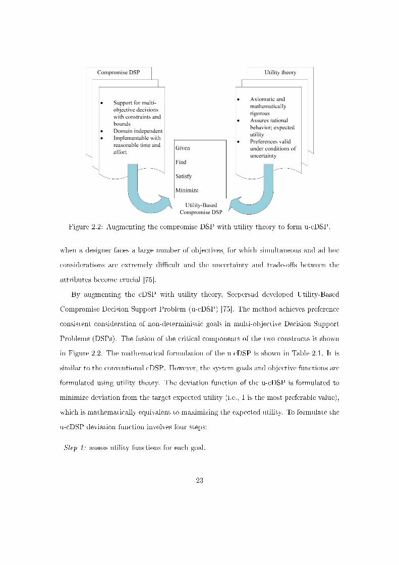
Figure 2.2: Augmenting the compromise DSP with utility theory to form u-cDSP.
when a designer faces a large number of objectives, for which simultaneous and ad hoc
considerations are extremely di�cult and the uncertainty and trade-o�s between the
attributes become crucial [75].
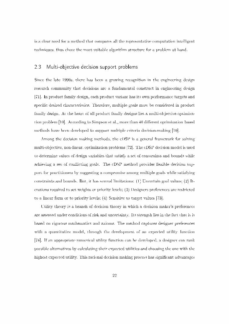
By augmenting the cDSP with utility theory, Seepersad developed Utility-Based
Compromise Decision Support Problem (u-cDSP) [75]. The method achieves preference
consistent consideration of non-deterministic goals in multi-objective Decision Support
Problems (DSPs). The fusion of the critical components of the two constructs is shown
in Figure 2.2. The mathematical formulation of the u-cDSP is shown in Table 2.1. It is
similar to the conventional cDSP. However, the system goals and objective functions are
formulated using utility theory. The deviation function of the u-cDSP is formulated to
minimize deviation from the target expected utility (i.e., 1 is the most preferable value),
which is mathematically equivalent to maximizing the expected utility. To formulate the
u-cDSP deviation function involves four steps:
Step 1: assess utility functions for each goal.
23
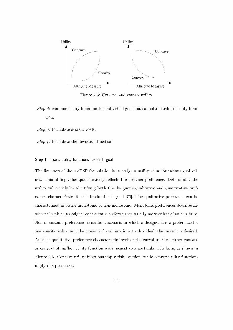
Figure 2.3: Concave and convex utility.
Step 2: combine utility functions for individual goals into a multi-attribute utility func-
tion.
Step 3: formulate system goals.
Step 4: formulate the deviation function.
Step 1: assess utility functions for each goal
The �rst step of the u-cDSP formulation is to assign a utility value for various goal val-
ues. This utility value quantitatively re�ects the designer preference. Determining the
utility value includes identifying both the designer's qualitative and quantitative pref-
erence characteristics for the levels of each goal [76]. The qualitative preference can be
characterized as either monotonic or non-monotonic. Monotonic preferences describe in-
stances in which a designer consistently prefers either strictly more or less of an attribute.
Non-monotonic preferences describe a scenario in which a designer has a preference for
one speci�c value, and the closer a characteristic is to this ideal, the more it is desired.
Another qualitative preference characteristic involves the curvature (i.e., either concave
or convex) of his/her utility function with respect to a particular attribute, as shown in
Figure 2.3. Concave utility functions imply risk aversion, while convex utility functions
imply risk proneness.
24
Table 2.1: Mathematical form of the utility-based compromise decision support problem.
Given: An alternative to be improved through modi�cation. Assumptions usedto model the domain of interest. The system parameters. All otherrelevant information.n number of system variablesp+ q number of system constraintsp equality constraintsq inequality constraintsm number of system goalsgi(X) system constraint functionAi(X) system goalsUi(Ai(X)) utility function for each goalU(X) overall, multi-attribute utility function
= f [u1(A1(X)), u2(A2(X)), ..., um(Am(X))]Find: The values of the independent system variables (that describe the phys-
ical attributes of an artifact).X = X1, ..., Xj j = 1, ..., nThe values of the deviation variables (that indicate the extent to whichtarget utilities are achieved).d−i , d
+i i = 1, ...,m
Satisfy: The system constraints that must be satis�ed for the solution to befeasible. There is no restriction place on linearity or convexity.gr(X) = 0 r = 1, ..., pgr(X)X ≥ 0 r = p+ 1, ..., p+ qThe system goals that must achieve a target utility to the extent possible.There is no restriction place on linearity or convexity.E[ui(Ai(X))] + d−i + d+
i = 1 i = 1, ...,mThe lower and upper bounds on the system variables.Xminj ≤ Xj ≤ Xmax
j j = 1, ..., n
d−i , d+i ≥ 0 and d−i · d
+i = 0
Minimize: The objective function:Case a: additive multi-attribute utility function
Z = 1− E[U(X)] =m∑i=1
ki(d−i + d+
i )
Case b: multiplicative multi-attribute utility function
Z = 1− E[U(X)] = 1− 1/K
(m∏i=1
[K ki E[ui(Ai(X))] + 1]
)− 1
= 1/K
(m∏i=1
[K ki(1− (d−i + d+i )) + 1]
)− 1
25
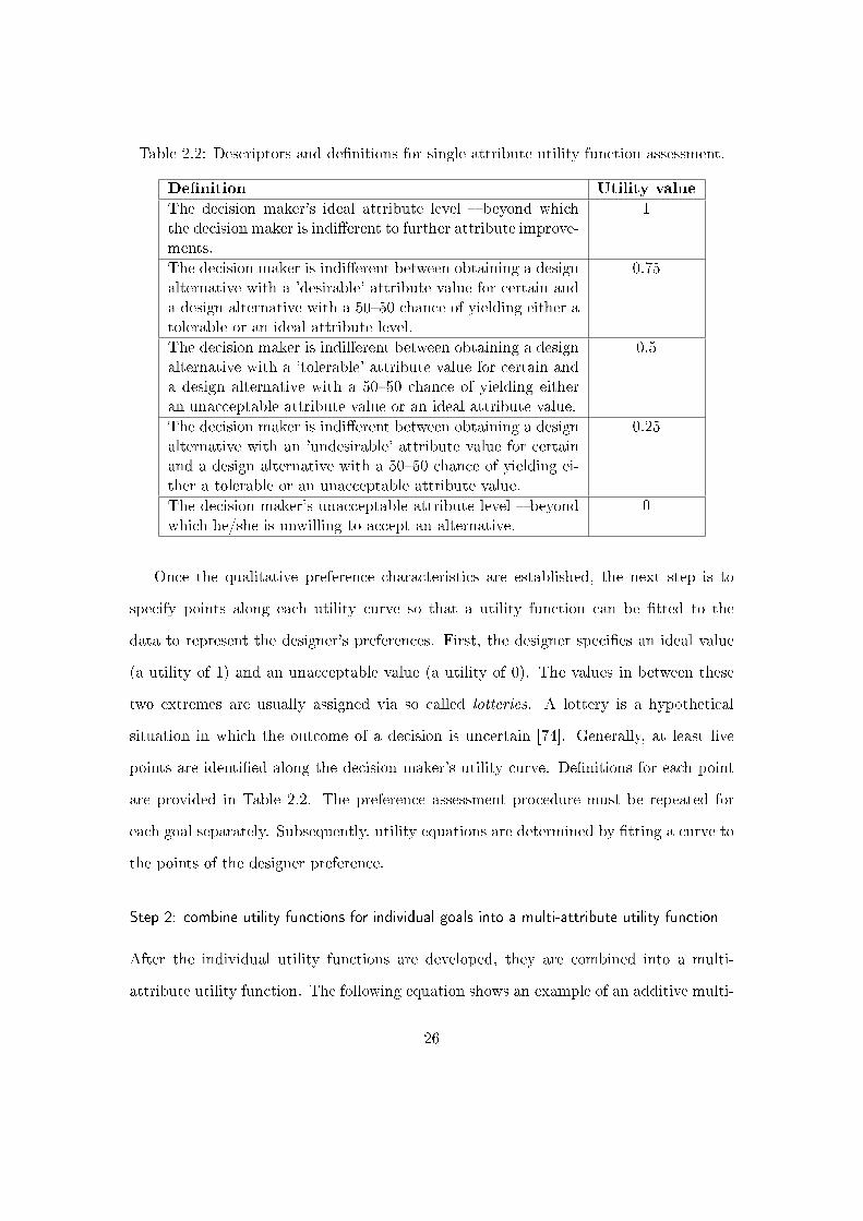
Table 2.2: Descriptors and de�nitions for single attribute utility function assessment.
De�nition Utility value
The decision maker's ideal attribute level � beyond whichthe decision maker is indi�erent to further attribute improve-ments.
1
The decision maker is indi�erent between obtaining a designalternative with a 'desirable' attribute value for certain anda design alternative with a 50�50 chance of yielding either atolerable or an ideal attribute level.
0.75
The decision maker is indi�erent between obtaining a designalternative with a 'tolerable' attribute value for certain anda design alternative with a 50�50 chance of yielding eitheran unacceptable attribute value or an ideal attribute value.
0.5
The decision maker is indi�erent between obtaining a designalternative with an 'undesirable' attribute value for certainand a design alternative with a 50�50 chance of yielding ei-ther a tolerable or an unacceptable attribute value.
0.25
The decision maker's unacceptable attribute level � beyondwhich he/she is unwilling to accept an alternative.
0
Once the qualitative preference characteristics are established, the next step is to
specify points along each utility curve so that a utility function can be �tted to the
data to represent the designer's preferences. First, the designer speci�es an ideal value
(a utility of 1) and an unacceptable value (a utility of 0). The values in between these
two extremes are usually assigned via so called lotteries. A lottery is a hypothetical
situation in which the outcome of a decision is uncertain [74]. Generally, at least �ve
points are identi�ed along the decision maker's utility curve. De�nitions for each point
are provided in Table 2.2. The preference assessment procedure must be repeated for
each goal separately. Subsequently, utility equations are determined by �tting a curve to
the points of the designer preference.
Step 2: combine utility functions for individual goals into a multi-attribute utility function
After the individual utility functions are developed, they are combined into a multi-
attribute utility function. The following equation shows an example of an additive multi-
26
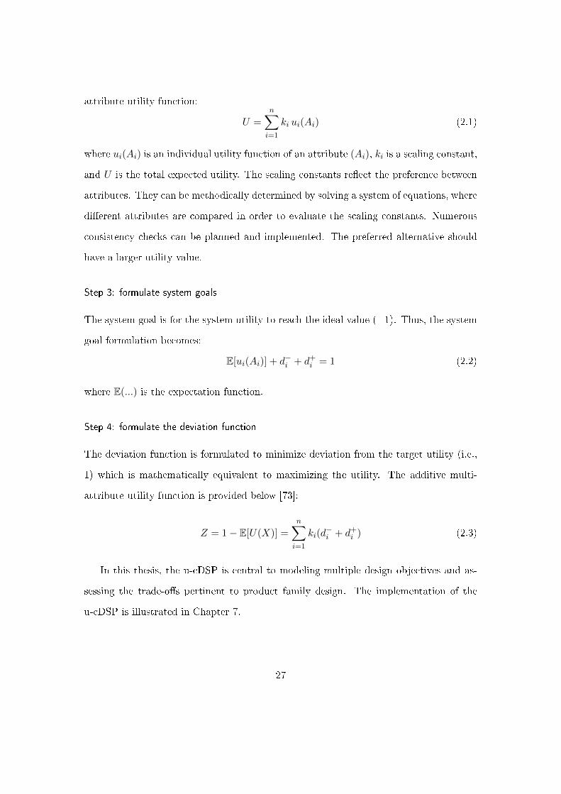
attribute utility function:
U =n∑i=1
ki ui(Ai) (2.1)
where ui(Ai) is an individual utility function of an attribute (Ai), ki is a scaling constant,
and U is the total expected utility. The scaling constants re�ect the preference between
attributes. They can be methodically determined by solving a system of equations, where
di�erent attributes are compared in order to evaluate the scaling constants. Numerous
consistency checks can be planned and implemented. The preferred alternative should
have a larger utility value.
Step 3: formulate system goals
The system goal is for the system utility to reach the ideal value (=1). Thus, the system
goal formulation becomes:
E[ui(Ai)] + d−i + d+i = 1 (2.2)
where E(...) is the expectation function.
Step 4: formulate the deviation function
The deviation function is formulated to minimize deviation from the target utility (i.e.,
1) which is mathematically equivalent to maximizing the utility. The additive multi-
attribute utility function is provided below [73]:
Z = 1− E[U(X)] =
n∑i=1
ki(d−i + d+
i ) (2.3)
In this thesis, the u-cDSP is central to modeling multiple design objectives and as-
sessing the trade-o�s pertinent to product family design. The implementation of the
u-cDSP is illustrated in Chapter 7.
27
2.4 Additive manufacturing facilitates customization
Many enterprises use product family design strategies to increase product customization
and reduce time to market while keeping the cost under control. The design of plat-
forms, within a product family, enables manufacturers to maintain the economic bene�ts
of having common parts and processes (reduced system complexity, reduced develop-
ment time and costs) while still being able to o�er variety to customers [15]. Thevenot
et al. [43] developed a product variety trade-o� evaluation method which helps design-
ers to balance all factors that determine platform commonality and individual product
performance within a product family. Jiao and Tseng [77] developed a product family
architecture model to handle the trade-o�s between diverse customer requirements, de-
sign re-usability and process capabilities. Martin and Ishii [40] introduced a design for
variety method, that includes the generational variety index and the coupling index, to
help reduce the design e�ort and time-to-market for products of a family. Williams et
al. [78] proposed an optimization-based platform design approach, called the augmented
product platform constructal theory method, which enables designers to systematically
manage modularity and commonality in the design of both product and process plat-
forms. Common to the aforementioned research work is the realization that a successful
product platform must balance the performance and commonality of individual products
in the family. However, performance and commonality are two con�icting objectives,
a sharing platform for all products in the family means to compromise in one way or
another. Furthermore, product variety induced manufacturing complexity has become
a signi�cant problem [44]. O�ering a�ordable customization is the foremost di�culty
that enterprises face when they follow the product family design paradigm. Most of
the product family design literature focuses on methodologies that optimize processes in
the traditional manufacturing technology context. However, new technology, especially
new manufacturing technology, can be a game changer. Porters was among the �rst
28
researchers who realized the transformational power of technology [21]. In his in�uential
work on competitive strategy, he suggested that technology is perhaps the most impor-
tant single source of major market share changes among competitors and it can lead to
the demise of an entrenched dominant �rm.
AM refers to the process of fabricating parts layer-by-layer directly from a Computer
Aided Design (CAD) model. AM production technique is clearly distinguished from
other conventional manufacturing techniques, such as machining (material removal) or
casting (deform material). Some common AM processes include Stereolithography (SL),
Fused Deposition Modeling (FDM), Selective Laser Sintering (SLS) and 3D printing.
These processes share some similarities, but they also have a number of distinguishing
properties. Initially, we introduce the common AM processes. More detailed reviews of
numerous AM technologies can be found in [79, 80].
The development of SL processes can be traced back to the mid-1980s. The process
produces parts one layer at a time by curing a photo-reactive resin with a Ultraviolet (UV)
laser or another similar power source. At present, 3D SystemsTM is the predominant
manufacturer of SL machines in the world. The two main advantages of SL technology
over other AM technologies are part accuracy and surface �nish, in combination with
average mechanical properties [81].
Powder Bed Fusion (PBF) processes were among the �rst commercialized AM pro-
cesses. Developed at the University of Texas at Austin, USA, SLS was the �rst com-
mercialized PBF process. The schematic in Figure 2.4 shows the its basic method of
operation. All PBF processes share a basic set of characteristics. These include one or
more thermal source for inducing the fusion between powder particles, a method for con-
trolling powder fusion to a prescribed region of each layer, and mechanisms for adding
and smoothing powder layers [79]. The SLS process works with a variety of thermo-
plastic materials, such as polyamide and Acrylonitrile Butadiene Styrene (ABS), it also
works with metal and ceramic powders. In PBF, the loose powder bed is a su�cient
29

Figure 2.4: Schematic of the SLS process.
support material for polymer PBF. This saves signi�cant time during part building and
post-processing, and enables advanced geometries that are di�cult to be post-processed
when supports are necessary. Accuracy and surface �nish of powder-based AM process
are typically inferior to liquid-based processes. However, accuracy and surface �nish are
strongly in�uenced by the operating conditions and the powder particle size. The ability
to nest polymer parts in 3-dimensions enables many parts to be produced in a single
build, thus dramatically improving the productivity of the PBF process when compared
with processes that require supports.
The FDM process, which is produced and developed by StratasysTM, uses a heating
chamber to liquefy a polymer that is fed into the system as a �lament. The �lament is
pushed into the chamber by a tractor wheel arrangement. The major strength of FDM
is in the range of materials that can be used for manufacturing and good mechanical
properties of the resulting parts. For example, parts made using FDM are amongst the
strongest for any polymer-based AM processes [79].
30
From the brief introduction above, it is clear that each AM process builds 3D objects
in layers, the means by which the layers are built di�er from method to method. With the
unique capabilities for fabricating components with high complexity in shape, function,
and material, AM technologies have greatly increased the design freedom in the product
development area [79]. Holmström et al. [82] suggested the unique characteristics of the
AM production lead to the following bene�ts:
� No tooling is needed, signi�cantly reducing production ramp-up time and expense.
� Small production batches are feasible and economical.
� Possibility to execute rapid design changes.
� Allows the product to be optimized for a speci�c function.
� Allows economical custom products (batch of one).
� Possibility to reduce waste.
� Potential for simpler supply chains; shorter lead times and lower inventories.
� Design customization.
Over the past two decades, the research community has developed novel AM pro-
cesses and applied them in the aerospace [83, 84], automotive [85] and biomedical [86]
�elds. These AM processes and applications di�er from each other in terms of stock
material types, material bonding mechanism, dimensional accuracies, post-processing re-
quirements, etc. [8]. The di�erences open up a wide range of options for product design-
ers. As a consequence, Rosen [87] puts forward that, in order to take advantage of these
unique technologies, we have to move to Design for Additive Manufacturing (DFAM)
from Design for Manufacture (DFM). The DFAM principles and strategies have been
explored in the literature. Gibson et al. [79] de�ned the goals of DFAM as �maximize
product performance through the synthesis of shapes, sizes, hierarchical structures, and
31
material compositions, subject to the capability of AM technologies". The de�nition
sparked lots of research and design studies related to AM. For example, Hague et al. [88]
studied and summarized design rules for SL and SLS, based on DFM guidelines for injec-
tion molding. They found that some DFM rules for injection molding are not applicable
to AM. In other words, AM overcomes many limitations of conventional manufacturing
processes. Su et al. [89] suggested a set of design guidelines of non-assembly mechanism
built in one piece using Selective Laser Melting (SLM). Maidin et al. [90] constructed a
design feature database for AM, which enabled users to visualize and gather information
in the conceptual design stage. Xu et al. [91] developed generic models to help the
designers select the most suitable AM process for a speci�c part creation.
The increased capabilities of AM techniques pave the way for optimized design ap-
proaches, such as topology optimization. In many cases, designs from topology optimiza-
tion, although optimal, may be impossible to manufacture with traditional manufacturing
methods. In recent years, topology optimization has emerged as a promising approach
to utilize the bene�ts of AM as manufacturing tool [92]. For example, Rezaie et al. [93]
developed a methodology which conceptualizes the application of topology optimization
to design parts built by FDM.
With AM technologies, a manufacturing cell that includes both fabrication and as-
sembly becomes possible. Furthermore, without tooling needs, AM processes could be
particularly interesting for practitioners of mass customization. For example, Siemens
Hearing Instruments, Inc. produces hearing aid shells that �t into individual ears us-
ing SL technology [94]. In 2007, the company claimed that about half of the in-the-ear
hearing aids, that it produced in the US, were fabricated using AM technologies. For
a consumer goods market, that deals with electronic devices, the electronics inside may
remain the same while the outside housing can be customized for a particular customer.
The manufacturing cost, associated with the customization, would be no higher than
the manufacturing cost of generic items. Production planing and control will become
32
much more important however � particularly in terms of the information technology sys-
tems. Instead of having to warehouse parts, and/or tooling, a manufacturer just needs
to maintain individual customer data and corresponding electronic design speci�cations.
However, the product data management challenge will be enormous.
Most of the existing research, related to AM, analyzed singular part designs, with a
special focus on geometric design freedom and limitations. There is limited research which
investigates the interrelation between AM and customization in product family design.
However, we have reasons to belief that the interrelation holds the key for improved
customization. As a consequence, there is a need for design models to bridge these
two paradigms such that they bene�t from each other in order to achieve a�ordable
customization in the product family development area.
2.5 Summary and preview
The role of Chapter 2 is to present, discuss and critically evaluate the building blocks
of a data-driven product family design method for AM. The discussions aim to explain
and justify the research challenges introduced in Chapter 1. The following list details
how the discussion in this chapter justi�ed and contributed to the theoretical structural
validation of the proposed method.
� Section 2.1 reviewed product family design methods and tools with a focus on
scalable product families. Section 2.2 critically reviewed DM and machine learning
techniques in the domain of product family design. We argued that these advanced
techniques are e�ective for information extraction and provide informed decision
making. The data-driven method is formalized into a Decision Support System
(DSS) for market segmentation and product positioning in Section 3.2.1. The
detailed method is implemented in Chapter 4, and validated in Chapter 5.
� Section 2.3 reviewed the DSP methods. The u-cDSP is employed as a mathematical
33

framework for modeling product family design decisions involving multiple objec-
tives in Section 3.2.3. The u-cDSP is formulated and solved for design of �nger
pump design in Chapter 7.
� Section 2.4 reviewed the state-of-the-art AM technologies. These enabling tech-
nologies are integrated to product family design process in Section 3.2.2 and it is
developed in Chapter 6 for customized cantilever beam family designs.
� The three building blocks are merged into the data-driven product family design
for AM. It is implemented and validated in Chapter 7.
In the next chapter, these constitutive elements are integrated to create the proposed
method.
34

Chapter 3
A data-driven product family design method
for additive manufacturing
Designing a product family in a dynamic contemporary environment requires us to re-
think the way how our creations provide value to customers over time. This chapter
elaborates on these thought processes and presents results to some of the most pressing
problems. The results center on data-driven product family design for Additive Manu-
facturing (AM). Section 3.2 introduces the details of the proposed method, along with
the employed tools. Section 3.3 concludes the chapter and with a look ahead to the
implementation of the proposed method and the example problems through Chapter 4
to Chapter 7.
3.1 Overview and rationale
This section links the research gaps, identi�ed in the literature review of Chapter 2, with
the research hypotheses put forward in Section 1.2. During the literature review, we
found that a successful product platform must balance performance and commonality
of individual products in the family. Performance and commonality are two con�icting
35

objectives, a shared platform for all products in the family means to establish an agree-
ment which resolves the con�ict. The way in which the agreement is reached depends
also on the product variety induced manufacturing complexity, because manufacturing
complexity is a signi�cant cost factor and sometimes there are hard technical limitations.
Therefore, o�ering product variety without compromising individual performance and re-
alizing product variants in a cost e�ective manner are challenging tasks that have to be
addressed. Our main hypothesis is that the data-driven product family design method
for AM has the ability to solve the problem. The following text highlights the novelty
of the main hypothesis. To be speci�c, we relate the re�ned sub-hypotheses to research
gaps identi�ed in the literature review.
In Section 2.2 of the literature review, we put forward that decisions on market seg-
mentation and product positioning are crucial for companies to meet diverse Customer
Needs (CNs) and achieve its goals. The successful development of Data Mining (DM)-
based knowledge discovery is a key issue to achieve objective decision support for market-
ing research problem-solving. However, the existing DM-based methods and techniques
were selected without a coherent strategy on an ad-hoc basis. We found every market
research problem requires us to establish a suitable algorithm structure, because di�er-
ent algorithms, for the same task, have di�erent merits and shortcomings. In order to
provide reliable decision support for market segmentation and product positioning, there
is a clear need for a method that compares all the representative computation intelligent
techniques, thus chose the most suitable algorithm structure for a problem at hand. To
solve that problem, we put forward our research sub-hypothesis 1:
Sub-hypothesis 1: A Decision Support System (DSS) that employs advanced
DM and machine learning techniques can be developed to help identify market
segmentation and predict product positioning.
In Section 2.4 of the literature review, we found that most of the product family design
literature focuses on methodologies that optimize processes in the traditional manufac-
36
turing technology context. However, new technology, such as AM, can be rede�ne the
way we think of o�ering customization for identi�ed market segments. In the AM lit-
erature, most of the research analyzed singular part designs, with a special focus on
geometric design freedom and limitations. There is limited research which investigates
the interrelation between AM and customization in product family design. However, we
have reasons to belief that the interrelation holds the key for improved customization.
As a consequence, there is a need for design models to bridge these two paradigms such
that they bene�t from each other in order to achieve a�ordable customization in the
product family development area. To solve that problem, we put forward our research
sub-hypothesis 2:
Sub-hypothesis 2: An AM process model for product family design can be
developed to incorporate AM into product family design process in order to
facilitate improved customization in target market segments.
Scalable product family designs pose multi-objective Decision Support Problems
(DSPs). To solve that problem, we put forward our research sub-hypothesis 3:
Sub-hypothesis 3: A utility-based compromise DSP can be formulated to
model multiple design objectives.
In order to substantiate the individual research hypotheses, we propose the data-
driven product family design method for AM. The method addresses the research gaps in
a logically and methodically re�ned way. The next section is dedicated to the introduction
of the method.
3.2 The method: data-driven product family design for additive manu-
facturing
This section introduces data-driven product family design for AM and it illustrates how
the proposed method addresses the research questions. By addressing the research ques-
tions, we validate the research hypotheses. Before we embark on outlining the details
37
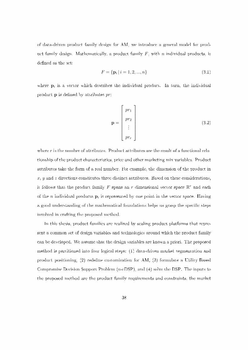
of data-driven product family design for AM, we introduce a general model for prod-
uct family design. Mathematically, a product family F , with n individual products, is
de�ned as the set:
F = {pi | i = 1, 2, ..., n} (3.1)
where pi is a vector which describes the individual product. In turn, the individual
product p is de�ned by attributes pr:
p =
pr1
pr2
...
prr
(3.2)
where r is the number of attributes. Product attributes are the result of a functional rela-
tionship of the product characteristics, price and other marketing mix variables. Product
attributes take the form of a real number. For example, the dimension of the product in
x, y and z directions constitutes three distinct attributes. Based on these considerations,
it follows that the product family F spans an r dimensional vector space Rr and each
of the n individual products pi is represented by one point in the vector space. Having
a good understanding of the mathematical foundations helps us grasp the speci�c steps
involved in crafting the proposed method.
In this thesis, product families are realized by scaling product platforms that repre-
sent a common set of design variables and technologies around which the product family
can be developed. We assume that the design variables are known a priori. The proposed
method is partitioned into four logical steps: (1) data-driven market segmentation and
product positioning, (2) rede�ne customization for AM, (3) formulate a Utility-Based
Compromise Decision Support Problem (u-cDSP), and (4) solve the DSP. The inputs to
the proposed method are the product family requirements and constraints, the market
38

Figure 3.1: Overview diagram of the data-driven product family design for AM method.
data, as well as the Design for Additive Manufacturing (DFAM) requirements and con-
straints. The output is the customized product family design. Four steps describe how to
formulate the problems and solve them. The sections below detail the individual steps.
Figure 3.1 shows the individual steps of the proposed method as well as the applied tools
and methods for each step.
3.2.1 Step 1: data-driven market segmentation and product positioning
The �rst step identi�es market segmentation and product positioning. The market seg-
mentation provides a link between management, marketing, and engineering design. It
helps decision makers identify which type of leveraging strategy can be used to meet
the overall design requirements and realize a suitable product family. The data from
39

Table 3.1: Market segmentation matrix.
Customer preferencesCluster 1 2 3 . . . N − 1 N
1(20%) G1
2(15%) G2
.... . .
n(10%) Gn
both consumers and competitors form the basis for market segmentation and product
positioning.
The market data that contains the needed information, i.e. the customer preference
data, is collected and standardized. The individual customers di�er in their perception of
product attributes. Thus the customer preferences can be represented by a set of product
attributes P = {prx|x = 1, 2, ..., r}. Suppose a total of N customer preference data
sets are analyzed with cluster-based DM methods. The clustering process identi�es the
preference data pattern, because the data structure is shaped by the CNs. The extracted
information represents customer groups that share the same or very similar value criteria.
The core idea revolves around the fact that we interpret the clustering result as market
segmentation. Based on the analysis, customers are isolated and grouped into n clusters,
as shown in Table 3.1. Mathematically, the market segmentation is represented as:
Gy|∀y = 1, 2, ..., n (3.3)
where n ≤ N , denote the market segments. Each market segment is related to a speci�c
set of product attributes P . By ordering the product attribute sets we form n product
vectors p which belong to the product family F .
40
In Table 3.1, the customers who belong to the same cluster have similar preference
for a speci�c product. Table 3.1 also provides useful information about the size of each
cluster. For example, 20% of the customer population for cluster 1, 15% for cluster 2
and 10% for cluster Gn. Consumer behavior studies suggest that the consumers falling
into the same cluster usually hold the same purchase trend and thus the customer can
be satis�ed by providing such a product that the total variations of functionality from
what the customer prefers are the smallest [95]. Furthermore, the information may be
used to help product con�guration and production capacity estimation.
Based on the market segmentation, machine learning techniques are employed to
provide decision support on product positioning. The product positions are in�uenced
directly by the product attributes. In order to objectify both market segmentation and
product positioning decisions, we develop a DSS that integrates powerful data manage-
ment with robust analytical methods into an intuitive Graphical User Interface (GUI).
We realized that every DSS problem requires a suitable algorithm structure, because
di�erent algorithms, for the same task, have di�erent merits and shortcomings and it
is impossible to know a priori which combination of algorithms gives the best results.
Therefore, to select the best algorithms is empirical science where the possible combi-
nations are tested. Therefore, the proposed DSS for market segmentation and product
positioning is partitioned into four subsystems including (1) data subsystem, (2) o�ine
model subsystem, (3) online model subsystem and (4) dialog subsystem. Figure 3.2 gives
the overview of the DSS. In the data subsystem, the data set, that contains the needed
information, is collected and stored. Data standardization and accessibility are a prereq-
uisite to realize the promise of DSS. Hence, a data conditioning software is employed to
build up database tables from the collected data set. The data subsystem o�ers robust,
reliable, and e�cient data storage and easy retrieval for large volumes of data. Based on
a user's need, the selected data from the the data subsystem will be fed into o�ine sub-
system. The o�ine subsystem performs clustering using representative DM and machine
41

Figure 3.2: A decision support system for market segmentation and product positioning.
learning techniques, and rigorously evaluates the clustering performance. Only the best
processing structure is chosen for the online subsystem active decision support on market
segmentation and product positioning. In the dialog subsystem, we integrate powerful
data management with robust analytical methods into an intuitive GUI, which ensures
a user barrier free access to decision support information. A detailed construction of the
proposed DSS is illustrated and validated in Chapters 4 and 5
3.2.2 Step 2: rede�ne customization for additive manufacturing
Once the market segmentation is identi�ed and the targeted market segments are chosen,
the next step is to de�ne a customization space and o�er customization to di�erent
market segments. The �space of customization� is de�ned as the set of all feasible value
combinations of product attributes that a manufacturing enterprise is willing to satisfy
42
[96]. It is de�ned by three components:
� Customization parameters to be o�ered. The number of parameters determines the
dimension of the customization space. For example, o�ering di�erent pump �ow
rates de�nes a one-dimension customization space.
� The range of each customization parameter. The range values are usually de�ned
by economic or technological limitations. The customization space is not limited
to continuous variables. It can be formed by continuous, discrete or mixed-valued
requirements. For example, pump �ow rate range from 100 ml/min to 1000 ml/min.
� The analysis of the demand of the targeted market segments.
As discussed in Section 2.4, AM technology provides more �exibility in product family
design when compared to traditional manufacturing methods. The unique properties
of AM will fundamentally alter considerations about commonality and customization
in product family design. With this enabling technology, the ultimate aim is to o�er
individual customization where the CNs are fully satis�ed. Due to the AM processes
restrictions, the DFAM guidelines have to be incorporated into to the product family
design process.
This step follows the DFAM guidelines that are developed by Gibson et al. [79].
� AM enables the usage of complex geometry in achieving design goals without in-
curring time or cost penalties compared with simple geometry.
� AM enables the usage of customized geometry and parts by direct production from
3D data.
� With AM, it is often possible to consolidate parts by integrating features into more
complex parts and avoiding assembly issues.
� AM allows designers to ignore all of the constraints imposed by conventional man-
ufacturing processes.
43
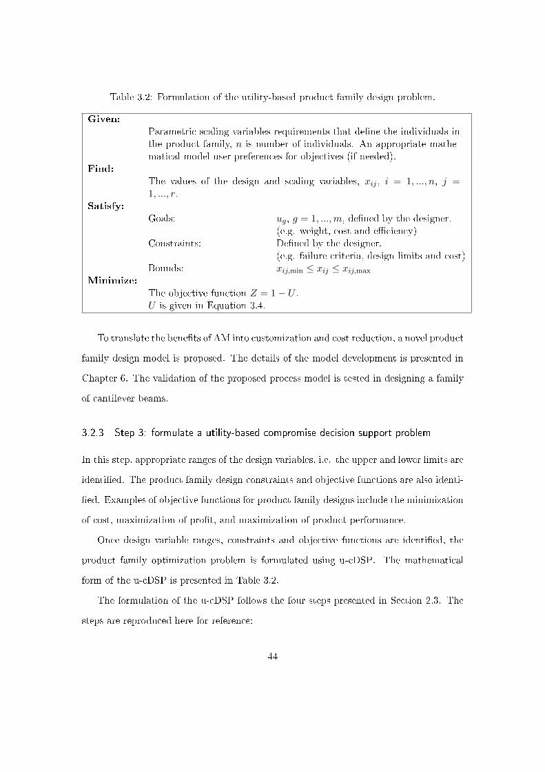
Table 3.2: Formulation of the utility-based product family design problem.
Given:
Parametric scaling variables requirements that de�ne the individuals inthe product family, n is number of individuals. An appropriate mathe-matical model user preferences for objectives (if needed).
Find:
The values of the design and scaling variables, xij , i = 1, ..., n, j =1, ..., r.
Satisfy:
Goals: ug, g = 1, ...,m, de�ned by the designer.(e.g. weight, cost and e�ciency)
Constraints: De�ned by the designer.(e.g. failure criteria, design limits and cost)
Bounds: xij,min ≤ xij ≤ xij,max
Minimize:
The objective function Z = 1− U .U is given in Equation 3.4.
To translate the bene�ts of AM into customization and cost reduction, a novel product
family design model is proposed. The details of the model development is presented in
Chapter 6. The validation of the proposed process model is tested in designing a family
of cantilever beams.
3.2.3 Step 3: formulate a utility-based compromise decision support problem
In this step, appropriate ranges of the design variables, i.e. the upper and lower limits are
identi�ed. The product family design constraints and objective functions are also identi-
�ed. Examples of objective functions for product family designs include the minimization
of cost, maximization of pro�t, and maximization of product performance.
Once design variable ranges, constraints and objective functions are identi�ed, the
product family optimization problem is formulated using u-cDSP. The mathematical
form of the u-cDSP is presented in Table 3.2.
The formulation of the u-cDSP follows the four steps presented in Section 2.3. The
steps are reproduced here for reference:
44
� Assess the utility functions for each goal. Initially, we have to identify the de-
signer's qualitative and quantitative preference characteristics for the �ve utility
value levels of each goal. Subsequently, we have to �t a utility function to the
designer's preferences based on the utility value levels of each goal. In this the-
sis, the designers' preferences for each objective are modeled as risk averse (i.e.,
preference to act conservatively by avoiding risks), because most designers, under
most circumstances, are risk averse. They prefer alternatives that o�er on-target
outcomes to those that have considerable chances of yielding undesirable results.
Once the identi�cation of preferences is done, each utility function is �t to the �ve
points assess according to Table 2.2.
� Combine utility functions for individual goals into a multi-attribute utility func-
tion. We suppose that both the utility independence and additive independence of
multiple goals hold true. Hence, a designer's risk aversion, for the utility levels of
a goal, is constant, regardless of the utility levels associated with other goals. Fur-
thermore, there are no interactions between the designer's preferences for di�erent
goals. In this case, the sum of the scaling constants of individual goals equals to 1,
that is:∑m
g=1 kg = 1. Therefore, the expected utility function is formulated as an
additive multi-attribute utility function, as shown in Equation 3.4.
U =m∑g=1
kg ug (3.4)
where kg is a scaling constant for the goal ug.
� Formulate system goals. The utility functions are normalized such that the result
values are within the range from 0 to 1 (with 1 corresponding to the most preferred
goal value, and 0 stands for the least preferred goal value). Therefore, the target
45
value in the goal formulation is 1. The system goal is formulated as:
E[ui(Ai)] + d−i + d+i = 1 (3.5)
� Formulate the deviation function. The deviation function is formulated to minimize
the deviation form the target utility (i.e. 1) which is mathematically equivalent to
maximizing the utility. The deviation function of additive multi-attribute utility
functions is formulated as follows:
Z = 1− E[U(X)] =
m∑i=1
ki(d−i + d+
i ) (3.6)
Chapter 7 illustrates the formulation of the u-cDSP in detail for the design of a �nger
pump family.
3.2.4 Step 4: solve the decision support problem
The �nal step is to obtain a solution for the multi-objective u-cDSP formulated in the
previous step. As discussed by Williams [97], there are two methods for analyzing the
design space: through continuous evaluation, or through numerical discretization of the
space. Though the continuous evaluation approach represents the most rigorous and ex-
act technique, it is limited by the need de�ned by the objective functions as well as the
requirement that the demand scenarios must be functions of the design speci�cations.
The requirement adds considerable complexity to the derivation of the objective func-
tions, and ultimately excludes the integration of objective or demand functions, because
they cannot be solved analytically. To circumvent these limitations, Williams proposes
a discrete analysis whereby the design space is approximated by multiple discrete points
across the space. We have adopted this approach for solve the multi-objective DSP.
There are several algorithms, such as exhaustive search, generalized reduced gradient,
46
and sequential quadratic programming, can be used to �nd the design solution. The ex-
haustive search algorithm locates the design solution with a minimum deviation function
value that satis�es all of the constraints and bounds. If a generalized reduced gradi-
ent algorithm was employed, then it is necessary to investigate whether the algorithm
converged and whether it converged to a desirable region of the design space. With an
exhaustive search, these investigations are not necessary. It is important to check that
the constraints on the deviation variables have been satis�ed. The exhaustive search al-
gorithms insure that the constraints are satis�ed. Therefore, we employed an exhaustive
search algorithm to �nd a solution for the example problem in Chapter 7.
3.3 Summary and preview
Product family design is a complex process involving intensive decision making activities.
It is of paramount importance to use e�ective methods which help designers make the
right decisions. The role of this chapter is to:
� Present the data-driven product family design for AM method. Both Chapters 4
and 5 use and evaluate DM as well as machine learning techniques extensively. It
is understood that the presented techniques don't exhaust all the possible ways
in which to identify market segmentation and product positioning. However, the
chapters provide a blue print on how to construct a framework for robust data-
driven decision support.
� Incorporate AM into the product family design methodology in order to facilitate
improved mass customization. A case of design a family of cantilever beams is
presented in Chapter 6. The key contribution is the infusion of AM into the product
family design process. Chapter 7 extends this idea further.
� Present the formulation of the u-cDSP. The details of how the u-cDSP can be
formulated, including the cost model for Selective Laser Sintering (SLS), are pre-
47

sented in Chapter 7. An empirical structure and permanences are presented and
benchmarked.
This chapter provides a comprehensive and well-de�ned framework to assist data-
driven decision making in the product family design. The following chapters illustrate
the data-driven product family design for AM method and evaluate the proposed method
with case studies.
48
Chapter 4
A data-driven decision support system for
market segmentation and product
positioning
Making sense of market data is of paramount importance for competitive companies that
seek to address diverse Customer Needs (CNs). Meaningful market data is necessarily
high dimensional and large in volume. As a consequence, human interpretation of such
data is error prone and time intensive. With the current state of information technol-
ogy, better methods for market data interpretation are based on Data Mining (DM) and
machine learning. In an attempt to harvest the analytical power of modern DM and
machine learning algorithms, we present a data-driven Decision Support System (DSS)
that mines important information from market data to identify market segments with-
out prede�ned ones, and it provides decision support for product positioning. Section
4.2 introduces the DM and machine learning techniques, including Principle Component
Analysis (PCA), K-means, and AdaBoost classi�cation, that construct the DSS for mar-
ket segmentation and product positioning. The DSS implements Step 1 of the proposed
49
method, as outlined in Chapter 3. Section 4.3 describes the automotive case study and
the instantiation of the DSS. The results are reported along with a discussion. Section
4.4 summarizes the case study and its role in the veri�cation and validation strategy for
the thesis.
4.1 Overview of the decision support system
Market segmentation and product positioning aims to establish the properties of products
a �rm should o�er to customers in speci�c market segments. Product design is concerned
with establishing the physical product characteristics [98]. Both product positioning
and product design are non-stationary processes, i.e. they change over time and they
in�uence each other in complex ways. Therefore, decision makers have to concurrently
consider, which (a) market segments to serve, (b) competitors to challenge, and (c)
product characteristics to select [99]. DM techniques, that assimilate training sets, based
upon available data, help us to identify market segments, but these techniques are unlikely
to provide support for decision problems in the area of product positioning and design.
The knowledge discovery for the design intentions and marketing strategies should be
modeled, such that they can be retained throughout the product development process
[100]. The knowledge discovery requires clear modeling techniques, which incorporate
advanced decision making tools and utilities for early design stage decision making [101].
DSS frameworks provide a modeling strategy by combining knowledge discovery and
automated decision making. In the early 1970s, DSSs were developed as a new type of
tools which integrate DM with arti�cial decision making [102]. Power de�ned a DSS as
�an interactive computer-based system or subsystem intended to help decision makers
use communication technologies, data, documents, knowledge and/or models to identify
and solve problems, complete decision process tasks, and make decisions� [103]. In the
early product design and development stage, it is di�cult to make precise and objective
50
decisions due to a lack of information. Eeckhout and De Bosschere put forward that
early design stage decision support tools can provide extremely valuable information for
designers and decision makers [104]. There are many approaches being used for engi-
neering design, such as Pugh's selection matrix [105], Analytic Hierarchy Process (AHP)
[106], Suh's axiomatic design [107] and design for six sigma [108]. These decision mak-
ing tools enable more accurate decision making even amidst uncertain conditions. The
ability to carry out robust decision making has improved both e�ciency and relevance
of modern DSSs. However, none of these methods attempt to set targets or select a
design concept utilizing an enterprise-level decision criterion. Quality Function Deploy-
ment (QFD) is designed as a tool to provide an enterprise-level view to engineering design
[109]. However, using only customer and competitor information to set targets without
consideration of the physics of engineering attribute interactions or other product objec-
tives, such as market size and potential pro�t, can result in targets that can never be
achieved in practice [110]. There are various DSSs were developed to provide decision
support in marketing research. For example, Chiu et al. developed a DSS for market
segmentation using DM and optimization methods, however, these decision aids stop at
the market segmentation step. Besharati et al. proposed a DSS for supporting the prod-
uct design selection process [111]. The method was based on purchase or non-purchase
decisions from customers and they did not consider competitors' products. Xu et al.
provided appropriate evaluation and decision tools for concurrent product development
[101]. Their method has value in academic research, but their approach lacks an intu-
itive user interface, hence applications in an industrial setting are limited. The literature
review shows that both DM and decision making algorithms are utilized in many �elds
of science and engineering. However, there is no dedicated DSS which integrates these
algorithms in a meaningful and trustworthy way to support market segmentation and
product positioning simultaneously. Therefore, there is a need for DSSs that provide
synergy early in the product development stage.
51
This chapter presents a DSS for market segmentation and product positioning. The
proposed system is based on the proposition that DM and decision support tools make
relevant market data directly available to decision makers. We achieve this goal by in-
tegrating powerful data management with robust analytical methods into an intuitive
Graphical User Interface (GUI), which ensures barrier free access to decision support
information. On the methodology side, our core idea revolves around the fact that we
interpret the result of clustering algorithms on market data as market segmentation.
Based on the market segmentation, we use machine learning to provide decision support
on product positioning and design. These two concepts objectify both market segmen-
tation and design decisions. To demonstrate the usefulness of the proposed DSS for
market segmentation and product positioning, we present a case study based on the US
automotive market in 2010.
4.2 The construction of the decision support system
This section describes the methods used in the proposed data-driven DSS for market
segmentation and product positioning. Figure 4.1 shows an overview block diagram of
the system. It is structured into two phases: I, data preparation; II, decision support
with the Decision Support System Database Explorer (DSSDB Explorer). Each of these
phases is realized as a separate software program written in Java [112]. On a functional
level, the system reads in market data and converts it to entries in database tables. The
next step employs PCA and K-means clustering to identify the market segments. An
AdaBoost classi�er is trained on these individual market segments, and subsequently it
is used to determine the market segment to which a new product design belongs. The
following subsections describe the algorithms and methods used in the implementation.
52
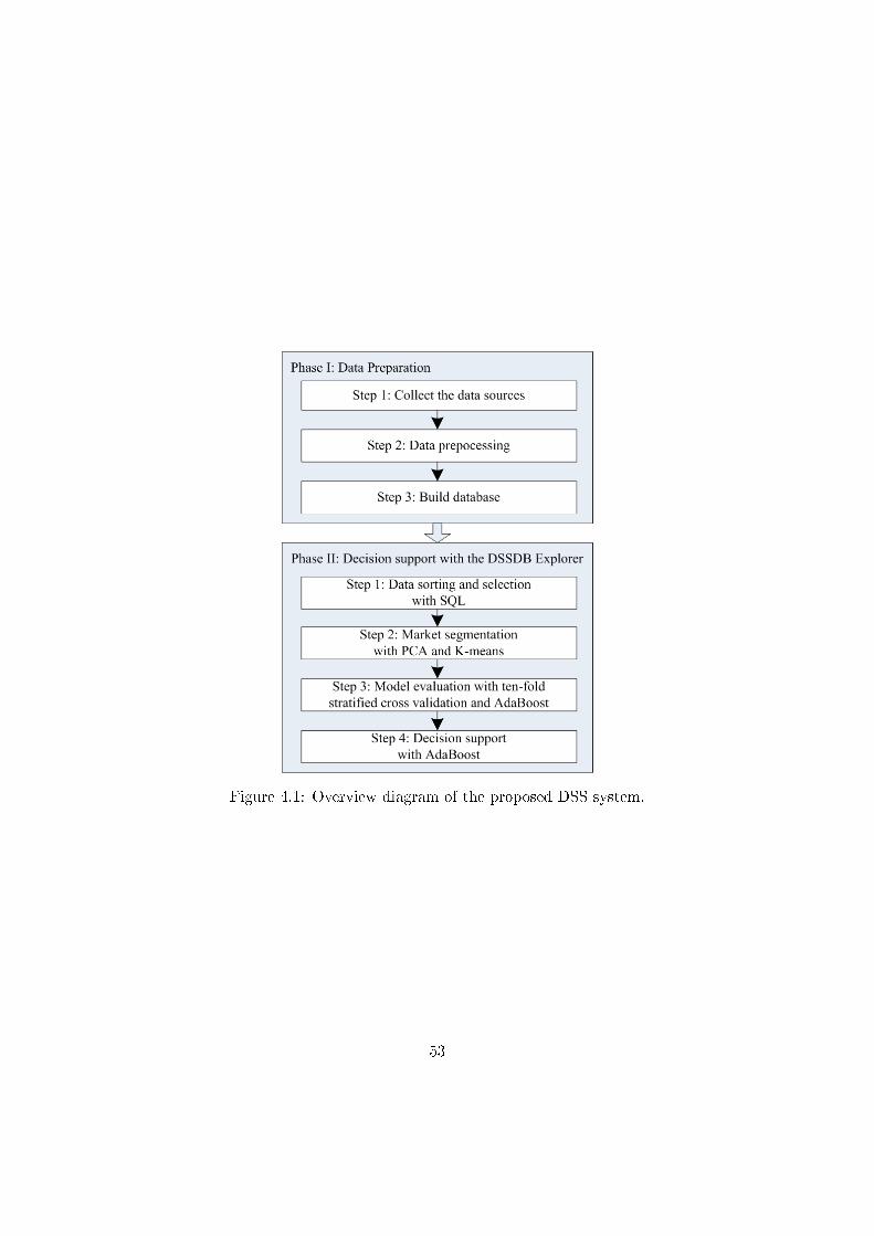
Figure 4.1: Overview diagram of the proposed DSS system.
53
4.2.1 Data preparation
Data standardization and accessibility are a prerequisite to realize the promise of DM.
In the data preparation phase, the data set, that contains the needed information, is
collected. Then a data conditioning software is employed to build up database tables
from the collected data set. These database tables o�er robust, reliable, and e�cient
data storage and easy retrieval for large volumes of data [113]. Therefore, they can be
used as a basis for DSSs, such as the proposed DSSDB Explorer [114].
4.2.2 Decision support with the DSSDB Explorer
This phase consists of four steps, as shown in Figure 4.1. The decision support process
starts with user driven data sorting and selection. On a technical level, this is realized
with Structured Query Language (SQL) statements and tabulated data display. Once
the data is chosen, the data analysis step employs PCA and K-means to identify the
market segments. Subsequently, the AdaBoost algorithm is used to build a classi�cation
model. This model decides to which market segment a new user de�ned data set belongs.
Strati�ed cross validation is used to evaluate the performance of the decision making
models. The next sections introduce the algorithms which were used to realize these
functions in a bottom-up way.
Principal Component Analysis (PCA)
PCA is a mathematical procedure that uses an orthogonal transformation to convert
a set of observations with possibly correlated variables into a set of values of linearly
uncorrelated variables called principal components [115]. The number of principal com-
ponents is less than or equal to the number of original variables. This transformation is
de�ned in such a way that the �rst principal component has the largest possible variance
(that is, accounts for as much of the variability in the data as possible), and each suc-
ceeding component in turn has the highest variance possible under the constraint that
54
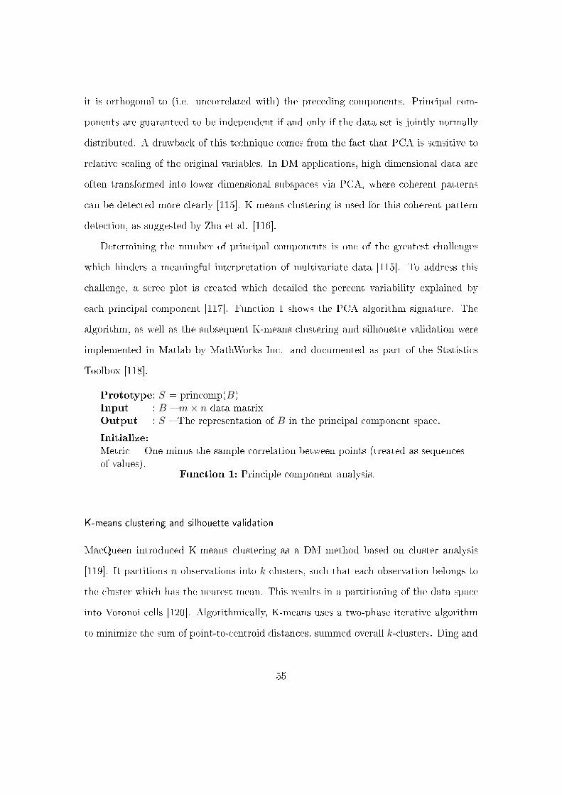
it is orthogonal to (i.e. uncorrelated with) the preceding components. Principal com-
ponents are guaranteed to be independent if and only if the data set is jointly normally
distributed. A drawback of this technique comes from the fact that PCA is sensitive to
relative scaling of the original variables. In DM applications, high dimensional data are
often transformed into lower dimensional subspaces via PCA, where coherent patterns
can be detected more clearly [115]. K-means clustering is used for this coherent pattern
detection, as suggested by Zha et al. [116].
Determining the number of principal components is one of the greatest challenges
which hinders a meaningful interpretation of multivariate data [115]. To address this
challenge, a scree plot is created which detailed the percent variability explained by
each principal component [117]. Function 1 shows the PCA algorithm signature. The
algorithm, as well as the subsequent K-means clustering and silhouette validation were
implemented in Matlab by MathWorks Inc. and documented as part of the Statistics
Toolbox [118].
Prototype: S = princomp(B)Input : B � m× n data matrixOutput : S � The representation of B in the principal component space.
Initialize:
Metric = One minus the sample correlation between points (treated as sequencesof values).
Function 1: Principle component analysis.
K-means clustering and silhouette validation
MacQueen introduced K-means clustering as a DM method based on cluster analysis
[119]. It partitions n observations into k clusters, such that each observation belongs to
the cluster which has the nearest mean. This results in a partitioning of the data space
into Voronoi cells [120]. Algorithmically, K-means uses a two-phase iterative algorithm
to minimize the sum of point-to-centroid distances, summed overall k-clusters. Ding and
55
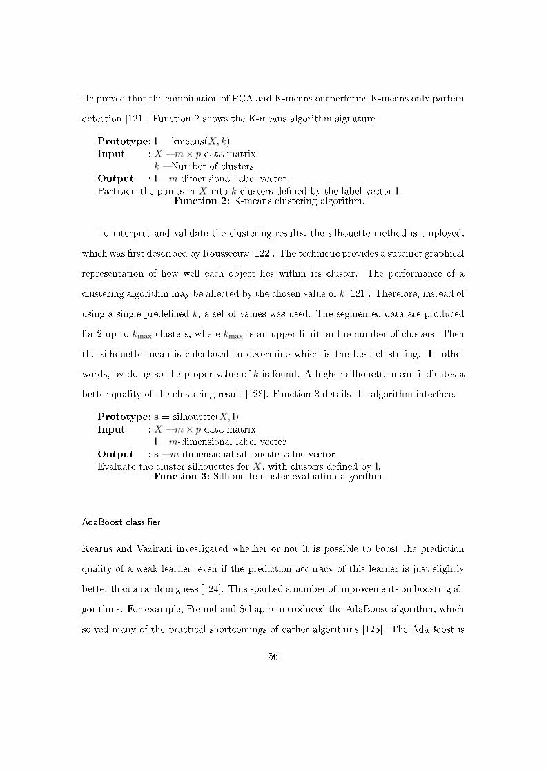
He proved that the combination of PCA and K-means outperforms K-means only pattern
detection [121]. Function 2 shows the K-means algorithm signature.
Prototype: l = kmeans(X, k)Input : X � m× p data matrix
k � Number of clustersOutput : l � m dimensional label vector.Partition the points in X into k clusters de�ned by the label vector l.
Function 2: K-means clustering algorithm.
To interpret and validate the clustering results, the silhouette method is employed,
which was �rst described by Rousseeuw [122]. The technique provides a succinct graphical
representation of how well each object lies within its cluster. The performance of a
clustering algorithm may be a�ected by the chosen value of k [121]. Therefore, instead of
using a single prede�ned k, a set of values was used. The segmented data are produced
for 2 up to kmax clusters, where kmax is an upper limit on the number of clusters. Then
the silhouette mean is calculated to determine which is the best clustering. In other
words, by doing so the proper value of k is found. A higher silhouette mean indicates a
better quality of the clustering result [123]. Function 3 details the algorithm interface.
Prototype: s = silhouette(X, l)Input : X � m× p data matrix
l � m-dimensional label vectorOutput : s � m-dimensional silhouette value vectorEvaluate the cluster silhouettes for X, with clusters de�ned by l.
Function 3: Silhouette cluster evaluation algorithm.
AdaBoost classi�er
Kearns and Vazirani investigated whether or not it is possible to boost the prediction
quality of a weak learner, even if the prediction accuracy of this learner is just slightly
better than a random guess [124]. This sparked a number of improvements on boosting al-
gorithms. For example, Freund and Schapire introduced the AdaBoost algorithm, which
solved many of the practical shortcomings of earlier algorithms [125]. The AdaBoost is
56
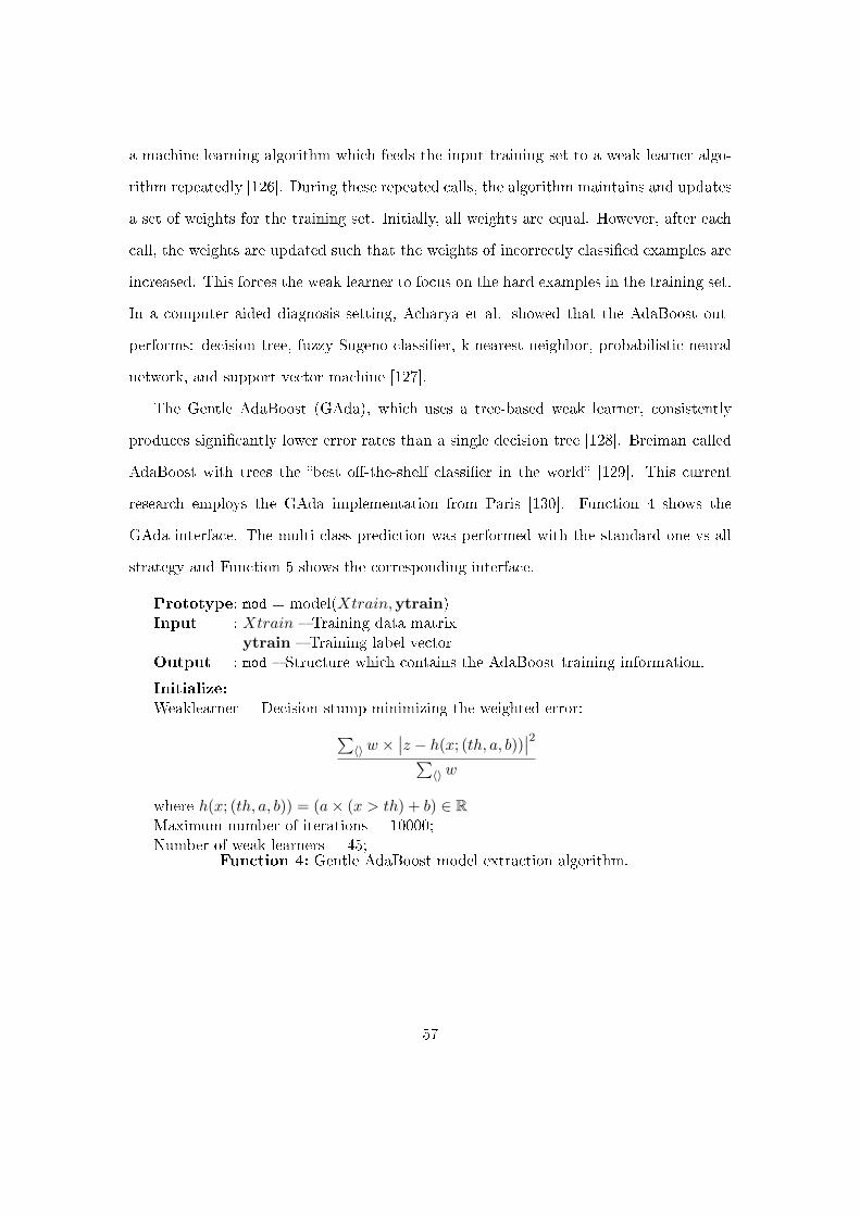
a machine learning algorithm which feeds the input training set to a weak learner algo-
rithm repeatedly [126]. During these repeated calls, the algorithm maintains and updates
a set of weights for the training set. Initially, all weights are equal. However, after each
call, the weights are updated such that the weights of incorrectly classi�ed examples are
increased. This forces the weak learner to focus on the hard examples in the training set.
In a computer aided diagnosis setting, Acharya et al. showed that the AdaBoost out-
performs: decision tree, fuzzy Sugeno classi�er, k-nearest neighbor, probabilistic neural
network, and support vector machine [127].
The Gentle AdaBoost (GAda), which uses a tree-based weak learner, consistently
produces signi�cantly lower error rates than a single decision tree [128]. Breiman called
AdaBoost with trees the �best o�-the-shelf classi�er in the world� [129]. This current
research employs the GAda implementation from Paris [130]. Function 4 shows the
GAda interface. The multi-class prediction was performed with the standard one-vs-all
strategy and Function 5 shows the corresponding interface.
Prototype: mod = model(Xtrain,ytrain)Input : Xtrain � Training data matrix
ytrain � Training label vectorOutput : mod � Structure which contains the AdaBoost training information.
Initialize:
Weaklearner = Decision stump minimizing the weighted error:∑〈〉w ×
∣∣z − h(x; (th, a, b))∣∣2∑
〈〉w
where h(x; (th, a, b)) = (a× (x > th) + b) ∈ RMaximum number of iterations = 10000;Number of weak learners = 45;
Function 4: Gentle AdaBoost model extraction algorithm.
57
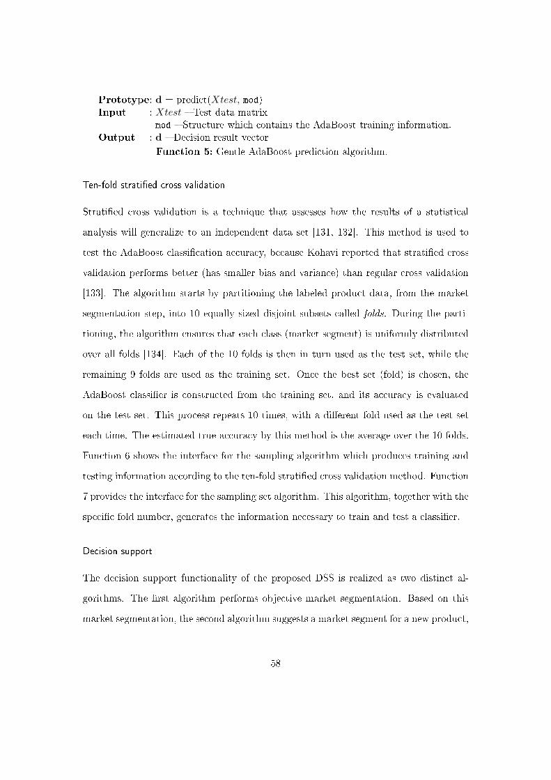
Prototype: d = predict(Xtest, mod)Input : Xtest � Test data matrix
mod � Structure which contains the AdaBoost training information.Output : d � Decision result vector
Function 5: Gentle AdaBoost prediction algorithm.
Ten-fold strati�ed cross validation
Strati�ed cross validation is a technique that assesses how the results of a statistical
analysis will generalize to an independent data set [131, 132]. This method is used to
test the AdaBoost classi�cation accuracy, because Kohavi reported that strati�ed cross
validation performs better (has smaller bias and variance) than regular cross validation
[133]. The algorithm starts by partitioning the labeled product data, from the market
segmentation step, into 10 equally sized disjoint subsets called folds. During the parti-
tioning, the algorithm ensures that each class (market segment) is uniformly distributed
over all folds [134]. Each of the 10 folds is then in turn used as the test set, while the
remaining 9 folds are used as the training set. Once the best set (fold) is chosen, the
AdaBoost classi�er is constructed from the training set, and its accuracy is evaluated
on the test set. This process repeats 10 times, with a di�erent fold used as the test set
each time. The estimated true accuracy by this method is the average over the 10 folds.
Function 6 shows the interface for the sampling algorithm which produces training and
testing information according to the ten-fold strati�ed cross validation method. Function
7 provides the interface for the sampling set algorithm. This algorithm, together with the
speci�c fold number, generates the information necessary to train and test a classi�er.
Decision support
The decision support functionality of the proposed DSS is realized as two distinct al-
gorithms. The �rst algorithm performs objective market segmentation. Based on this
market segmentation, the second algorithm suggests a market segment for a new product,
58
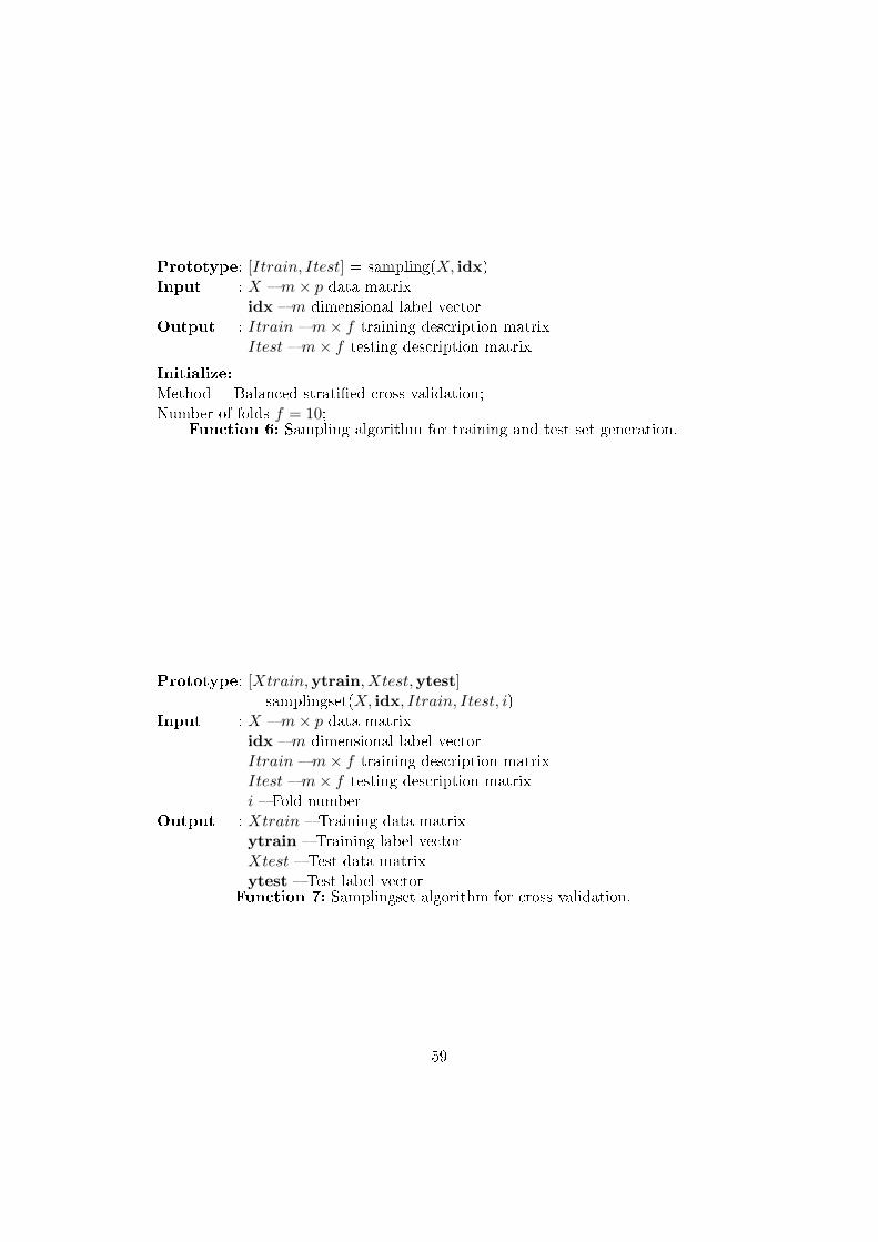
Prototype: [Itrain, Itest] = sampling(X, idx)Input : X � m× p data matrix
idx � m dimensional label vectorOutput : Itrain � m× f training description matrix
Itest � m× f testing description matrix
Initialize:
Method = Balanced strati�ed cross validation;Number of folds f = 10;
Function 6: Sampling algorithm for training and test set generation.
Prototype: [Xtrain,ytrain, Xtest,ytest]= samplingset(X, idx, Itrain, Itest, i)
Input : X � m× p data matrixidx � m dimensional label vectorItrain � m× f training description matrixItest � m× f testing description matrixi � Fold number
Output : Xtrain � Training data matrixytrain � Training label vectorXtest � Test data matrixytest � Test label vector
Function 7: Samplingset algorithm for cross validation.
59

which is described by a set of product properties.
The pseudocode of Function 8 describes the analysis algorithm that determines the
market segmentation from a given set of market data A. The algorithm normalizes A
before PCA is used to transform the high dimensional data into a lower dimensional
data X. The next step analyzes how well X clusters. To be speci�c, the loop shown
in Line 4. of Function 8 analyzes 2 to kmax = 16 clusters which were generated with
K-means and assessed with the silhouette tests. Line 5. of the algorithm determines the
cluster-con�guration with the highest silhouette area (idx) and this cluster-con�guration
will be used for the subsequent ten-fold strati�ed cross validation step. The loop, shown
in Line 7., traverses through the 10 folds. Each of these folds is used to train and test the
AdaBoost classi�er. Line 7. (d) evaluates the performance of the individual folds. The
accumulative mean classi�cation accuracy of the individual folds constitutes the ten-fold
cross validated classi�er performance r. For the proposed DSS, this parameter provides a
quality measure for the market segmentation step, which is implemented as the analysis
algorithm.
The second algorithm of the proposed DSS suggests a market segment for a given
set of product properties. To realize this functionality the algorithm, shown in Function
9, uses the AdaBoost classi�er to determine to which cluster the test vector belongs.
Line 1. of Function 9 extends the data matrix A by adding the test vector as the last
row. After normalization, the �rst m rows of the lower dimensional matrix X are used
to train the classi�er. Once the classi�er is trained, the last row of X is used for testing.
Combining data matrix and test vector ensures consistency as well as data integrity. The
result of the decision support step d can be interpreted as the speci�c market position of
the new product.
60

Prototype: [idx, r]=analysis(A)Input : A � m× n data matrixOutput : idx � m dimensional label vector
r � Test error
1. B = Standardized version of A, such that the ns of A are centered to have mean 0and scaled to have standard deviation 1;
2. S = princomp(B);
3. X = S(:,1:3);
4. for k = 2, 3, ..., kmax do
(a) lk = kmeans(X, k);
(b) s = silhouette(X, lk);
(c) msk = mean(s);
end
5. idx = lmax(ms);
6. [Itrain, Itest] = sampling(X, idx);
7. for i = 1, 2, ..., 10 do
(a) [Xtrain,ytrain, Xtest,ytest] =samplingset(X, idx, Itrain, Itest, i);
(b) mod = model(Xtrain,ytrain);
(c) d = predict(Xtest, mod);
(d)
ei =∑〈〉
di <> ytestif
where f is the dimension of d as well as ytest and
a <> b =
{0 if a = b
1 else
end
8. r=mean(e);
Function 8: Analysis algorithm to establish the data quality.
61
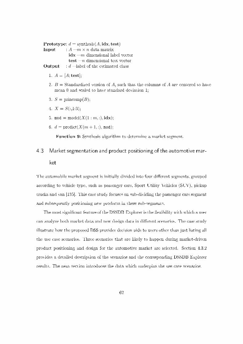
Prototype: d = synthesis(A, idx, test)Input : A � m× n data matrix
idx � m dimensional label vectortest � n dimensional test vector
Output : d � label of the estimated class
1. A = [A; test];
2. B = Standardized version of A, such that the columns of A are centered to havemean 0 and scaled to have standard deviation 1;
3. S = princomp(B);
4. X = S(:,1:3);
5. mod = model(X(1 : m, :), idx);
6. d = predict(X(m+ 1, :), mod);
Function 9: Synthesis algorithm to determine a market segment.
4.3 Market segmentation and product positioning of the automotive mar-
ket
The automobile market segment is initially divided into four di�erent segments, grouped
according to vehicle type, such as passenger cars, Sport Utility Vehicles (SUV), pickup
trucks and van [135]. This case study focuses on sub-dividing the passenger cars segment
and subsequently positioning new products in these sub-segments.
The most signi�cant feature of the DSSDB Explorer is the �exibility with which a user
can analyze both market data and new design data in di�erent scenarios. The case study
illustrate how the proposed DSS provides decision aids to users other than just listing all
the use case scenarios. Three scenarios that are likely to happen during market-driven
product positioning and design for the automotive market are selected. Section 4.3.2
provides a detailed description of the scenarios and the corresponding DSSDB Explorer
results. The next section introduces the data which underpins the use case scenarios.
62
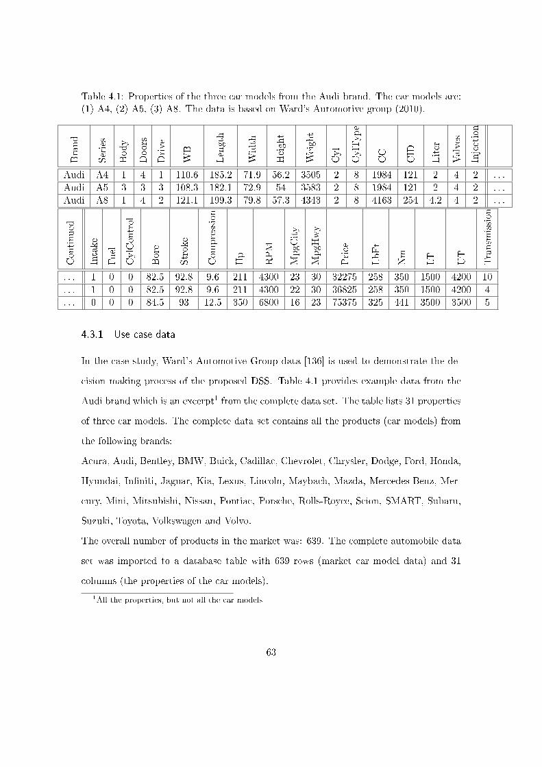
Table 4.1: Properties of the three car models from the Audi brand. The car models are:(1) A4, (2) A5, (3) A8. The data is based on Ward's Automotive group (2010).
Brand
Series
Body
Doors
Drive
WB
Length
Width
Height
Weight
Cyl
CylType
CC
CID
Liter
Valves
Injection
Audi A4 1 4 1 110.6 185.2 71.9 56.2 3505 2 8 1984 121 2 4 2 . . .
Audi A5 3 3 3 108.3 182.1 72.9 54 3583 2 8 1984 121 2 4 2 . . .
Audi A8 1 4 2 121.1 199.3 79.8 57.3 4343 2 8 4163 254 4.2 4 2 . . .
Continued
Intake
Fuel
CylControl
Bore
Stroke
Com
pression
Hp
RPM
MpgC
ity
MpgH
wy
Price
LbFt
Nm
LT
UT
Transm
ission
. . . 1 0 0 82.5 92.8 9.6 211 4300 23 30 32275 258 350 1500 4200 10
. . . 1 0 0 82.5 92.8 9.6 211 4300 22 30 36825 258 350 1500 4200 4
. . . 0 0 0 84.5 93 12.5 350 6800 16 23 75375 325 441 3500 3500 5
4.3.1 Use case data
In the case study, Ward's Automotive Group data [136] is used to demonstrate the de-
cision making process of the proposed DSS. Table 4.1 provides example data from the
Audi brand which is an excerpt1 from the complete data set. The table lists 31 properties
of three car models. The complete data set contains all the products (car models) from
the following brands:
Acura, Audi, Bentley, BMW, Buick, Cadillac, Chevrolet, Chrysler, Dodge, Ford, Honda,
Hyundai, In�niti, Jaguar, Kia, Lexus, Lincoln, Maybach, Mazda, Mercedes-Benz, Mer-
cury, Mini, Mitsubishi, Nissan, Pontiac, Porsche, Rolls-Royce, Scion, SMART, Subaru,
Suzuki, Toyota, Volkswagen and Volvo.
The overall number of products in the market was: 639. The complete automobile data
set was imported to a database table with 639 rows (market car model data) and 31
columns (the properties of the car models).
1All the properties, but not all the car models
63
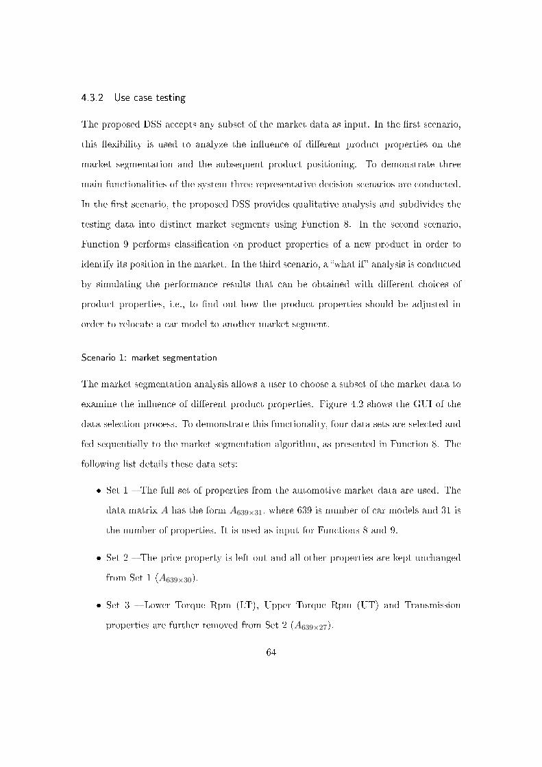
4.3.2 Use case testing
The proposed DSS accepts any subset of the market data as input. In the �rst scenario,
this �exibility is used to analyze the in�uence of di�erent product properties on the
market segmentation and the subsequent product positioning. To demonstrate three
main functionalities of the system three representative decision scenarios are conducted.
In the �rst scenario, the proposed DSS provides qualitative analysis and subdivides the
testing data into distinct market segments using Function 8. In the second scenario,
Function 9 performs classi�cation on product properties of a new product in order to
identify its position in the market. In the third scenario, a �what if� analysis is conducted
by simulating the performance results that can be obtained with di�erent choices of
product properties, i.e., to �nd out how the product properties should be adjusted in
order to relocate a car model to another market segment.
Scenario 1: market segmentation
The market segmentation analysis allows a user to choose a subset of the market data to
examine the in�uence of di�erent product properties. Figure 4.2 shows the GUI of the
data selection process. To demonstrate this functionality, four data sets are selected and
fed sequentially to the market segmentation algorithm, as presented in Function 8. The
following list details these data sets:
� Set 1 � The full set of properties from the automotive market data are used. The
data matrix A has the form A639×31, where 639 is number of car models and 31 is
the number of properties. It is used as input for Functions 8 and 9.
� Set 2 � The price property is left out and all other properties are kept unchanged
from Set 1 (A639×30).
� Set 3 � Lower Torque Rpm (LT), Upper Torque Rpm (UT) and Transmission
properties are further removed from Set 2 (A639×27).
64
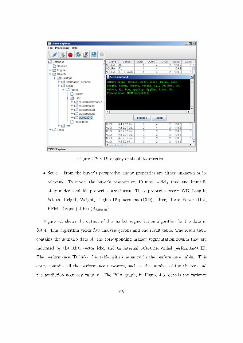
Figure 4.2: GUI display of the data selection.
� Set 4 � From the buyer's perspective, many properties are either unknown or ir-
relevant. To model the buyer's perspective, 10 most widely used and immedi-
ately understandable properties are chosen. These properties were: WB, Length,
Width, Height, Weight, Engine Displacement (CID), Liter, Horse Power (Hp),
RPM, Torque (LbFt) (A639×10).
Figure 4.3 shows the output of the market segmentation algorithm for the data in
Set 4. This algorithm yields �ve analysis graphs and one result table. The result table
contains the scenario data A, the corresponding market segmentation results that are
indicated by the label vector idx, and an internal reference, called performance ID.
The performance ID links this table with one entry in the performance table. This
entry contains all the performance measures, such as the number of the clusters and
the prediction accuracy value r. The PCA graph, in Figure 4.3, details the variance
65
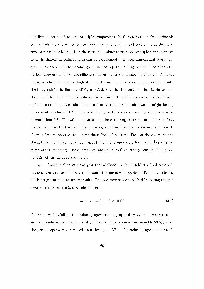
distribution for the �rst nine principle components. In this case study, three principle
components are chosen to reduce the computational time and cost while at the same
time preserving at least 80% of the variance. Taking these three principle components as
axis, the dimension reduced data can be represented in a three dimensional coordinate
system, as shown in the second graph in the top row of Figure 4.3. The silhouette
performance graph shows the silhouette mean versus the number of clusters. For data
Set 4, six clusters show the highest silhouette mean. To support this important result,
the last graph in the �rst row of Figure 4.3 depicts the silhouette plot for six clusters. In
the silhouette plot, silhouette values near one mean that the observation is well placed
in its cluster; silhouette values close to 0 mean that that an observation might belong
to some other cluster [122]. The plot in Figure 4.3 shows an average silhouette value
of more than 0.8. The value indicates that the clustering is strong, most market data
points are correctly classi�ed. The clusters graph visualizes the market segmentation. It
allows a human observer to inspect the individual clusters. Each of the car models in
the automotive market data was mapped to one of these six clusters. Area 1O shows the
result of this mapping. The clusters are labeled C0 to C5 and they contain 73, 138, 72,
62, 212, 82 car models respectively.
Apart from the silhouette analysis, the AdaBoost, with ten-fold strati�ed cross val-
idation, was also used to assess the market segmentation quality. Table 4.2 lists the
market segmentation accuracy results. The accuracy was established by taking the test
error r, from Function 8, and calculating:
accuracy = (1− r)× 100% (4.1)
For Set 1, with a full set of product properties, the proposed system achieved a market
segment prediction accuracy of 76.4%. The prediction accuracy increased to 93.5% when
the price property was removed from the input. With 27 product properties in Set 3,
66
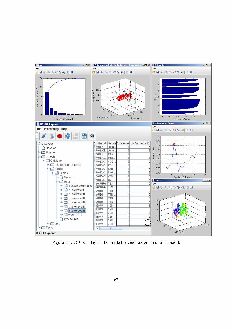
Figure 4.3: GUI display of the market segmentation results for Set 4.
67
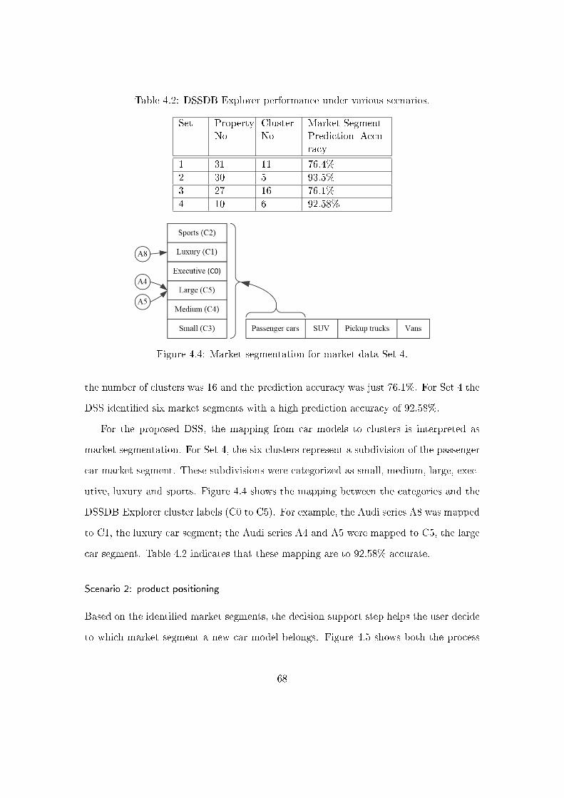
Table 4.2: DSSDB Explorer performance under various scenarios.
Set PropertyNo
ClusterNo
Market SegmentPrediction Accu-racy
1 31 11 76.4%
2 30 5 93.5%
3 27 16 76.1%
4 10 6 92.58%
Figure 4.4: Market segmentation for market data Set 4.
the number of clusters was 16 and the prediction accuracy was just 76.1%. For Set 4 the
DSS identi�ed six market segments with a high prediction accuracy of 92.58%.
For the proposed DSS, the mapping from car models to clusters is interpreted as
market segmentation. For Set 4, the six clusters represent a subdivision of the passenger
car market segment. These subdivisions were categorized as small, medium, large, exec-
utive, luxury and sports. Figure 4.4 shows the mapping between the categories and the
DSSDB Explorer cluster labels (C0 to C5). For example, the Audi series A8 was mapped
to C1, the luxury car segment; the Audi series A4 and A5 were mapped to C5, the large
car segment. Table 4.2 indicates that these mapping are to 92.58% accurate.
Scenario 2: product positioning
Based on the identi�ed market segments, the decision support step helps the user decide
to which market segment a new car model belongs. Figure 4.5 shows both the process
68
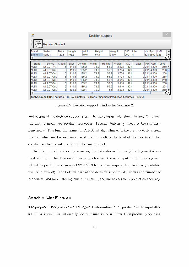
Figure 4.5: Decision support window for Scenario 2.
and output of the decision support step. The table input �eld, shown in area 2O, allows
the user to input new product properties. Pressing button 1O executes the synthesis
Function 9. This function trains the AdaBoost algorithm with the car model data from
the individual market segments. And then it predicts the label of the new input that
constitutes the market position of the new product.
In this product positioning scenario, the data shown in area 2O of Figure 4.5 was
used as input. The decision support step classi�ed the new input into market segment
C1 with a prediction accuracy of 92.58%. The user can inspect the market segmentation
results in area 3O. The bottom part of the decision support GUI shows the number of
properties used for clustering, clustering result, and market segment prediction accuracy.
Scenario 3: �what if� analysis
The proposed DSS provides market segment information for all products in the input data
set. This crucial information helps decision makers to customize their product properties.
69
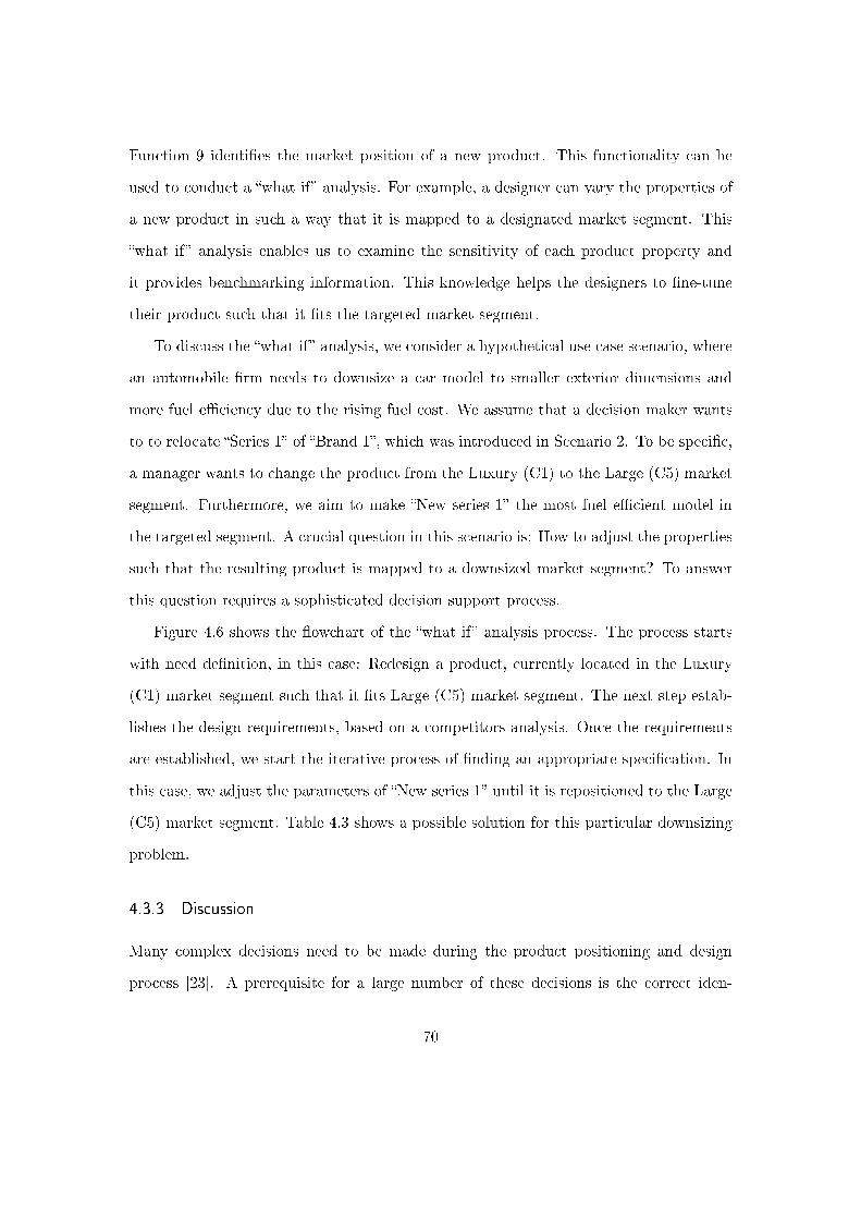
Function 9 identi�es the market position of a new product. This functionality can be
used to conduct a �what if� analysis. For example, a designer can vary the properties of
a new product in such a way that it is mapped to a designated market segment. This
�what if� analysis enables us to examine the sensitivity of each product property and
it provides benchmarking information. This knowledge helps the designers to �ne-tune
their product such that it �ts the targeted market segment.
To discuss the �what if� analysis, we consider a hypothetical use case scenario, where
an automobile �rm needs to downsize a car model to smaller exterior dimensions and
more fuel e�ciency due to the rising fuel cost. We assume that a decision maker wants
to to relocate �Series 1� of �Brand 1�, which was introduced in Scenario 2. To be speci�c,
a manager wants to change the product from the Luxury (C1) to the Large (C5) market
segment. Furthermore, we aim to make �New series 1� the most fuel e�cient model in
the targeted segment. A crucial question in this scenario is: How to adjust the properties
such that the resulting product is mapped to a downsized market segment? To answer
this question requires a sophisticated decision support process.
Figure 4.6 shows the �owchart of the �what if� analysis process. The process starts
with need de�nition, in this case: Redesign a product, currently located in the Luxury
(C1) market segment such that it �ts Large (C5) market segment. The next step estab-
lishes the design requirements, based on a competitors analysis. Once the requirements
are established, we start the iterative process of �nding an appropriate speci�cation. In
this case, we adjust the parameters of �New series 1� until it is repositioned to the Large
(C5) market segment. Table 4.3 shows a possible solution for this particular downsizing
problem.
4.3.3 Discussion
Many complex decisions need to be made during the product positioning and design
process [23]. A prerequisite for a large number of these decisions is the correct iden-
70
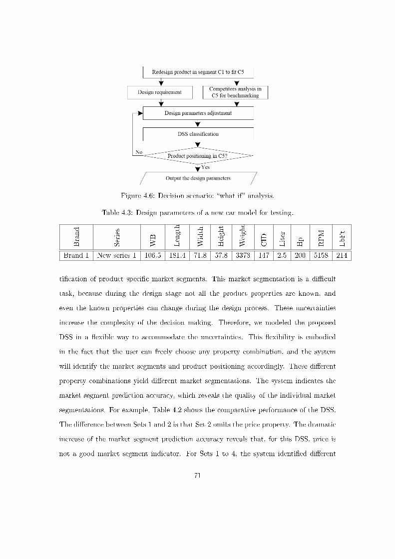
Figure 4.6: Decision scenario: �what if� analysis.
Table 4.3: Design parameters of a new car model for testing.
Brand
Series
WB
Length
Width
Height
Weight
CID
Liter
Hp
RPM
LbFt
Brand 1 New series 1 106.5 181.4 71.8 57.8 3373 147 2.5 200 5158 214
ti�cation of product speci�c market segments. This market segmentation is a di�cult
task, because during the design stage not all the product properties are known, and
even the known properties can change during the design process. These uncertainties
increase the complexity of the decision making. Therefore, we modeled the proposed
DSS in a �exible way to accommodate the uncertainties. This �exibility is embodied
in the fact that the user can freely choose any property combination, and the system
will identify the market segments and product positioning accordingly. These di�erent
property combinations yield di�erent market segmentations. The system indicates the
market segment prediction accuracy, which reveals the quality of the individual market
segmentations. For example, Table 4.2 shows the comparative performance of the DSS.
The di�erence between Sets 1 and 2 is that Set 2 omits the price property. The dramatic
increase of the market segment prediction accuracy reveals that, for this DSS, price is
not a good market segment indicator. For Sets 1 to 4, the system identi�ed di�erent
71

number of clusters with di�erent prediction accuracies. The results suggest that there
is a non-linear relationship between the number of properties and the market segment
prediction accuracy. But the results show an inverse relationship between amount of
clusters and the market segment prediction accuracy. This last point is understandable
because, decision support tools, such as the proposed DSSDB Explorer, perform better
when they have to deal with fewer signal classes [137].
To make better decisions on product positioning and design, it is necessary to con-
currently consider the changing customer needs and the entry or changed strategy of
the competitors [13]. The proposed DSS evaluates the market segments based on avail-
able market data, as this market data changes over time, so does the objective market
segmentation step in the DSSDB Explorer. This adaptive adjustment helps keep track
of vital information in dynamic market places. The resulting information can bene�t
enterprise decision making in a number of ways [138]. First, it allows the �rm to identify
segments with signi�cant opportunities. Second, through examination of di�erent mar-
ket segment results and current product portfolios, the decision makers can identify gaps
in their products, thus creating a justi�cation for developing new products. Also, the
product positioning result helps the �rm to strategically position their products in the
targeted segments. Furthermore, the proposed DSS can be used in �what if� scenarios,
where the new product properties are altered and the outcome of the market segment
decision is observed. Another bene�t is that the proposed DSS works even with incom-
plete parameters, that means all the bene�ts listed above can be realized early in the
design phase.
A brief summary and preview is given in the next section to close this chapter.
72
4.4 Summary and preview
The need for complex decision making, combined with the emergence of powerful infor-
mation systems, give rise to sophisticated DSSs. This chapter introduces the data-driven
DSS for market segmentation and product positioning. The proposed system combines
the reliability and accessibility of database entries with DM and machine learning meth-
ods. The GUI dialog system manages and coordinates the interaction between a user (a
decision maker), model and data, so that the decision maker receives barrier free sup-
port to solve product positioning and design problems. The proposed system identi�es
market segments and provides objective decision aids for product positioning and design.
Furthermore, the decision makers can use the system to model di�erent use scenarios
and conduct �what if� analysis.
By using real world market data, the proposed system works accurately in a practical
setting, even when there was just subset of the design data available. Therefore, enterprise
decision makers can obtain valuable decision support even in an early design phase.
The proposed DSS obtained 93.5% market segment prediction accuracy, in classifying
unknown product properties into one of the �ve market segments, with 30 out of 31
properties. This result was obtained with ten-fold strati�ed cross validation. The fact
that the high accuracy was achieved with this strict validation method makes us con�dent
that the proposed DSS can handle complex real world decision making situations. The
proposed system identi�es the market segments and suggests a speci�c market segment
for the new product design. The enabling techniques, such as market segmentation,
product positioning and �what if� analysis, ensure that the decision making processes
is conducted in an objective and systematic manner. Therefore, the proposed system
enables a �rm to tailor new products for speci�c market segments.
The limitations of the proposed DSS come from the ideas of objectivity. The funda-
mental problem is that even digital processing machinery is not entirely objective. These
73
machines have been built by humans to do speci�c tasks, i.e. a classi�er is build according
to speci�c rules and parameters to mimic human decision making. Furthermore, these
machines act on speci�c input data, but this data is selected according to subjective
criteria. For the case study, we used automotive data from Ward's Automotive Group,
a division of Penton Media Inc. (2010) and the decision to use this data was entirely
subjective. Another limitation of this work is that it did not include a way to rank the
individual input parameters. For example, human experts place lots of emphasis on the
price in contrast our system treats all input parameters with equal importance. The
reason why this weighting feature is absent comes from the fact that data weighting is
subjective and our aim was to produce a system which is as objective as possible. In other
words, weighting the input data would lead to market segmentation and subsequently to
decision support which is very much dependent on human experts. But this dependence
would limit the usefulness of the proposed system, because these human expert decisions,
which rely on weighting the input data, are not transferable between di�erent markets.
In this particular case, the proposed DSS works for any market where appropriate market
data is available with a minimum of subjective human intervention. The high prediction
accuracy makes us con�dent that the proposed DSS can provide useful information for
a wide range decision makers.
This chapter shows how the data-driven method can provide objective decision sup-
port for market segmentation and product positioning. Though the proposed DSS has
the aforementioned advantages, some questions remain unanswered.
� The selection of the DM techniques employed in the proposed DSS seems arbitrary,
even though it turned out the prediction accuracy of the system is pretty high for
this particular case study decision support problem. But is the combination of the
PCA, K-means and GAda algorithms the best way to form the DSS? Would an
alternative DSS design yield higher prediction accuracy?
74

� What will be the more robust and reliable way to construct a data-driven DSS for
market segmentation and product positioning?
The next chapter aims to shed some light on these unanswered questions, by providing
an extensive investigation into the tools and methods for data-driven market segmenta-
tion and product positioning. The investigation leads to a framework which answers how
to construct a robust DSS.
75
Chapter 5
Data-driven decision support system design
and evaluation
This chapter augments the data-driven Decision Support System (DSS) for market seg-
mentation and product design in Chapter 4. We focus on the o�ine and online subsystem
construction as well as testing of the proposed DSS, as shown in Figure 3.2 in Section
3.2.1. Every DSS problem requires us to search a suitable algorithm structure, because
di�erent algorithms, for the same task, have di�erent merits and shortcomings and it
is impossible to know a priory which combination of algorithms gives the best results.
Therefore, to select the best algorithms is empirical science where the possible combi-
nations are tested. The o�ine subsystem evaluates di�erent algorithms and selects the
best processing structure for the online subsystem. The rigorous evaluation and selection
process ensures reliable decision support from the DSS.
Section 5.1 reviews the data-driven product family design problems. Section 5.2
introduces the tools and techniques used in the construction of the o�ine and online
subsystems. In Section 5.3, these systems are tested and validated based on the same
example as in the previous chapter. The subsequent discussion section relates the �ndings
to the wider research on data-driven methods. Section 5.4 puts forward the summary of
76
the chapter.
5.1 Overview of data-driven decision support system design problems
In recent years, both scienti�c applications and business practices have become increas-
ingly data-intensive [139]. In today's competitive economy, information is central to the
enterprise's capacity to act [66]. Information, extracted from data, is a key element which
enables competitive companies to design successful products for a global market [140].
But, the fundamental question is: How do we extract this information from potentially
vast amounts of data? Questions like this gave rise to Data Mining (DM), which describes
a collection of methods and algorithms to extract information from data. However, DM
does not interpret the data, it just delivers information as a condensed form of raw data.
It is up to managers to make sense of this information and to use it as a basis for decisions.
This need for subjective interpretation leaves room for biased decisions which are prone
to baseline errors and informal fallacies [141]. As a result, complex product development
problems require decision aids, such as Decision Support Systems (DSSs). A DSS aims
to assist managers to make strategic decisions or predict future consequences by taking
into account the actual outcomes/performance of the enterprise's historical and current
marketing data. One way of constructing such a DSS is to combine DM methods with
machine learning for automated decision making.
DM is used to extract relevant information from data and machine learning uses this
information to create new insights, i.e. speculate about or predict the future trends
and model complex systems based on design variables [142]. One of the most critical
issues in engineering design is making decisions on a sound basis in the early design
stage [143]. In the product design process, a necessary design task is to make a decision
among candidate designs or parametric values, after the design has been formalized [144].
Data-driven approaches are gaining popularity within the enterprise as the amount of
77
available data increases in tandem with market pressures [139]. These approaches make
valuable and critical decisions traceable and repeatable. Brynjolfsson et al. found that
output and productivity of the �rms that adopt data-driven management increased 5�
6% [145]. The success of the data-driven approach relies on the quality of the gathered
data, the e�ectiveness of data analysis and the objectiveness of results interpretation.
Most of the evaluation criteria focus on ease of use, cost and capabilities of the systems
[146]. The computerized DSSs are designed to �reduce human error�. However, Skitka
et al. pointed out that an unreliable support aid might have disastrous consequences for
a company [147]. To overcome this problem, a reliable DSS must focus on properties,
such as accuracy, ease of use, cost and capabilities of the system [146]. Therefore, the
evaluation and subsequent selection of the DSS algorithms and methods is crucial for all
computerized DSSs.
This chapter describes the design of a robust DSS for market segmentation and prod-
uct positioning. It focuses on the systems design methodology and the algorithm eval-
uation. Our main contribution is that we structured the DSS into o�ine and online
subsystems, where the o�ine subsystem evaluates and selects the best processing struc-
ture for the online subsystem active decision support. To show the feasibility of the pro-
posed method, we discuss a DSS for product positioning in the automotive market. The
proposed system uses DM methods to extract market segmentation information from au-
tomotive market data and machine learning algorithms use this information to determine
the market segment of a new product. The o�ine subsystem compared (1) four intrinsic
dimension estimation techniques: Eigenvalue-based Estimator (EVE), Maximum Likeli-
hood Estimator (MLE), Correlation Dimension Estimator (CDE) and Geodesic Minimum
Spanning Tree (GMST), (2) three dimension reduction techniques: Local Linear Embed-
ding (LLE), Principle Component Analysis (PCA) and Multidimensional Scaling (MDS),
and (3) three clustering techniques: cluster, Fuzzy C-Means (FCM) and K-means. These
DM techniques were evaluated by measuring the cluster deviation, the silhouette mean
78
and the 10-fold cross validated accuracy of three automated classi�cation algorithms:
Gentle AdaBoost (GAda), Nearest Neighbor (NN) and Support Vector Machine (SVM).
For the proposed DSS, the SVM delivers the highest and most consistent classi�cation
accuracy.
5.2 Design and evaluation of the decision support system
This section focuses on the construction of the o�ine and online subsystems. The o�ine
subsystem evaluates the merits of both algorithms and a system structure. In this par-
ticular case, the results include the best dimension reduction algorithm, the best cluster
algorithm and the training model from the best classi�cation algorithm. These results are
used in the online subsystem to determine the market segment of a new product. Figure
5.1 shows the block diagram of the proposed DSS and the information transfer from the
o�ine to the online subsystems. The input for the o�ine subsystem is the high dimen-
sional data from the data subsystem. The intrinsic dimension estimation step estimates
the data dimensionality. The following dimension reduction step reduces the data to
this estimated dimension. The clustering algorithms extract structural information from
the new structured data set. The robust tests determine how valuable the information
is for a particular problem. In the online subsystem, the best algorithms for dimension
reduction, clustering and classi�cation are used to deliver the decision support to the
decision maker. The following sections detail the DM and machine learning techniques
which are employed in the proposed systems.
5.2.1 Intrinsic dimensionality estimation
There is a consensus in the high dimensional data analysis community that many types
of real life high dimensional data is embedded in a high-dimensional space. They can
be e�ciently summarized in a much lower dimension space without losing much infor-
79
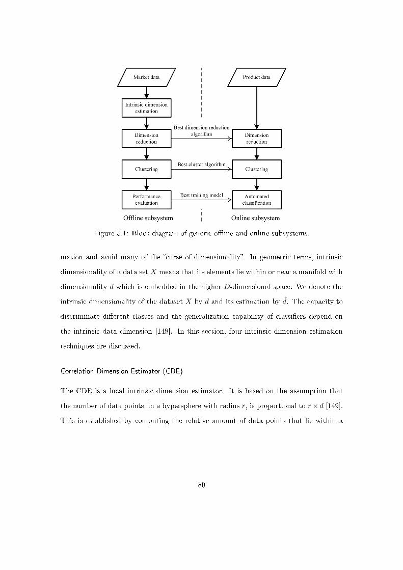
Figure 5.1: Block diagram of generic o�ine and online subsystems.
mation and avoid many of the �curse of dimensionality�. In geometric terms, intrinsic
dimensionality of a data set X means that its elements lie within or near a manifold with
dimensionality d which is embedded in the higher D-dimensional space. We denote the
intrinsic dimensionality of the dataset X by d and its estimation by d̂. The capacity to
discriminate di�erent classes and the generalization capability of classi�ers depend on
the intrinsic data dimension [148]. In this section, four intrinsic dimension estimation
techniques are discussed.
Correlation Dimension Estimator (CDE)
The CDE is a local intrinsic dimension estimator. It is based on the assumption that
the number of data points, in a hypersphere with radius r, is proportional to r× d [149].
This is established by computing the relative amount of data points that lie within a
80
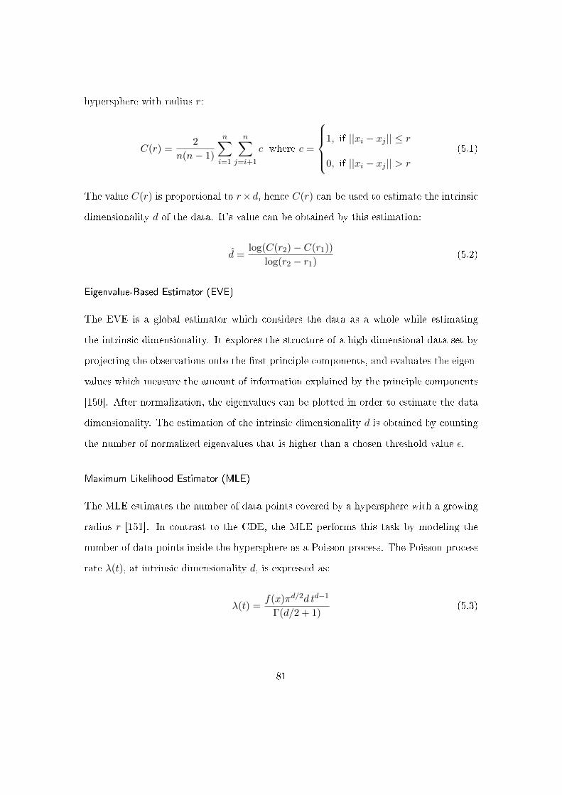
hypersphere with radius r:
C(r) =2
n(n− 1)
n∑i=1
n∑j=i+1
c where c =
1, if ||xi − xj || ≤ r
0, if ||xi − xj || > r
(5.1)
The value C(r) is proportional to r× d, hence C(r) can be used to estimate the intrinsic
dimensionality d of the data. It's value can be obtained by this estimation:
d̂ =log(C(r2)− C(r1))
log(r2 − r1)(5.2)
Eigenvalue-Based Estimator (EVE)
The EVE is a global estimator which considers the data as a whole while estimating
the intrinsic dimensionality. It explores the structure of a high-dimensional data set by
projecting the observations onto the �rst principle components, and evaluates the eigen-
values which measure the amount of information explained by the principle components
[150]. After normalization, the eigenvalues can be plotted in order to estimate the data
dimensionality. The estimation of the intrinsic dimensionality d is obtained by counting
the number of normalized eigenvalues that is higher than a chosen threshold value ε.
Maximum Likelihood Estimator (MLE)
The MLE estimates the number of data points covered by a hypersphere with a growing
radius r [151]. In contrast to the CDE, the MLE performs this task by modeling the
number of data points inside the hypersphere as a Poisson process. The Poisson process
rate λ(t), at intrinsic dimensionality d, is expressed as:
λ(t) =f(x)πd/2d td−1
Γ(d/2 + 1)(5.3)
81
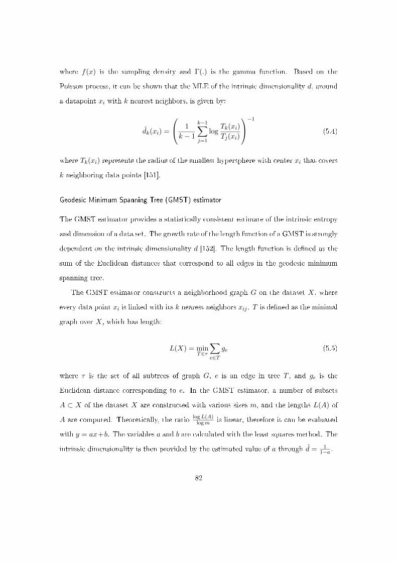
where f(x) is the sampling density and Γ(.) is the gamma function. Based on the
Poisson process, it can be shown that the MLE of the intrinsic dimensionality d, around
a datapoint xi with k nearest neighbors, is given by:
d̂k(xi) =
1
k − 1
k−1∑j=1
logTk(xi)
Tj(xi)
−1
(5.4)
where Tk(xi) represents the radius of the smallest hypersphere with center xi that covers
k neighboring data points [151].
Geodesic Minimum Spanning Tree (GMST) estimator
The GMST estimator provides a statistically consistent estimate of the intrinsic entropy
and dimension of a data set. The growth rate of the length function of a GMST is strongly
dependent on the intrinsic dimensionality d [152]. The length function is de�ned as the
sum of the Euclidean distances that correspond to all edges in the geodesic minimum
spanning tree.
The GMST estimator constructs a neighborhood graph G on the dataset X, where
every data point xi is linked with its k nearest neighbors xij . T is de�ned as the minimal
graph over X, which has length:
L(X) = minT∈τ
∑e∈T
ge (5.5)
where τ is the set of all subtrees of graph G, e is an edge in tree T , and ge is the
Euclidean distance corresponding to e. In the GMST estimator, a number of subsets
A ⊂ X of the dataset X are constructed with various sizes m, and the lengths L(A) of
A are computed. Theoretically, the ratio logL(A)logm is linear, therefore it can be evaluated
with y = ax+b. The variables a and b are calculated with the least squares method. The
intrinsic dimensionality is then provided by the estimated value of a through d̂ = 11−a .
82
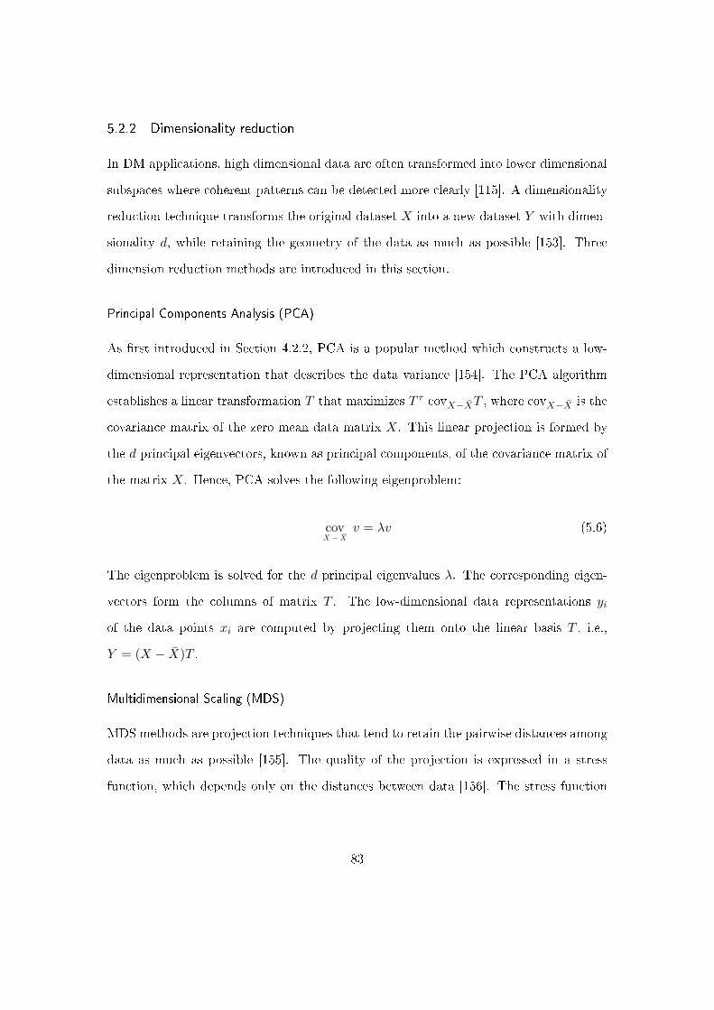
5.2.2 Dimensionality reduction
In DM applications, high dimensional data are often transformed into lower dimensional
subspaces where coherent patterns can be detected more clearly [115]. A dimensionality
reduction technique transforms the original dataset X into a new dataset Y with dimen-
sionality d, while retaining the geometry of the data as much as possible [153]. Three
dimension reduction methods are introduced in this section.
Principal Components Analysis (PCA)
As �rst introduced in Section 4.2.2, PCA is a popular method which constructs a low-
dimensional representation that describes the data variance [154]. The PCA algorithm
establishes a linear transformation T that maximizes T τ covX−X̄T , where covX−X̄ is the
covariance matrix of the zero mean data matrix X. This linear projection is formed by
the d principal eigenvectors, known as principal components, of the covariance matrix of
the matrix X. Hence, PCA solves the following eigenproblem:
covX − X̄
v = λv (5.6)
The eigenproblem is solved for the d principal eigenvalues λ. The corresponding eigen-
vectors form the columns of matrix T . The low-dimensional data representations yi
of the data points xi are computed by projecting them onto the linear basis T , i.e.,
Y = (X − X̄)T .
Multidimensional Scaling (MDS)
MDS methods are projection techniques that tend to retain the pairwise distances among
data as much as possible [155]. The quality of the projection is expressed in a stress
function, which depends only on the distances between data [156]. The stress function
83
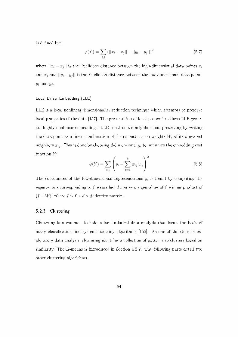
is de�ned by:
ϕ(Y ) =∑i j
(||xi − xj || − ||yi − yj ||)2 (5.7)
where ||xi − xj || is the Euclidean distance between the high-dimensional data points xi
and xj and ||yi − yj || is the Euclidean distance between the low-dimensional data points
yi and yj .
Local Linear Embedding (LLE)
LLE is a local nonlinear dimensionality reduction technique which attempts to preserve
local properties of the data [157]. The preservation of local properties allows LLE gener-
ate highly nonlinear embeddings. LLE constructs a neighborhood preserving by writing
the data point as a linear combination of the reconstruction weights Wi of its k nearest
neighbors xij . This is done by choosing d-dimensional yi to minimize the embedding cost
function Y :
ϕ(Y ) =∑〈i〉
yi − k∑j=1
wij yij
2
(5.8)
The coordinates of the low-dimensional representations yi is found by computing the
eigenvectors corresponding to the smallest d non-zero eigenvalues of the inner product of
(I −W ), where I is the d× d identity matrix.
5.2.3 Clustering
Clustering is a common technique for statistical data analysis that forms the basis of
many classi�cation and system modeling algorithms [158]. As one of the steps in ex-
ploratory data analysis, clustering identi�es a collection of patterns to clusters based on
similarity. The K-means is introduced in Section 4.2.2. The following parts detail two
other clustering algorithms.
84
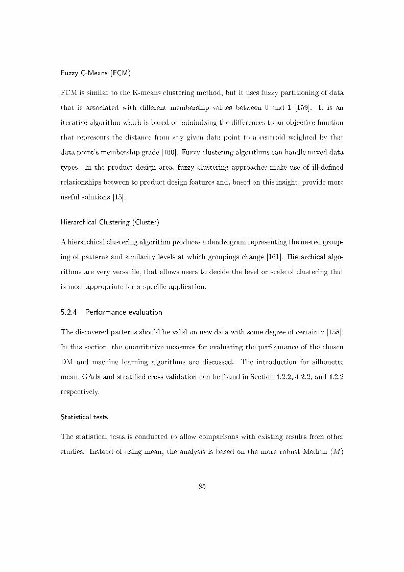
Fuzzy C-Means (FCM)
FCM is similar to the K-means clustering method, but it uses fuzzy partitioning of data
that is associated with di�erent membership values between 0 and 1 [159]. It is an
iterative algorithm which is based on minimizing the di�erences to an objective function
that represents the distance from any given data point to a centroid weighted by that
data point's membership grade [160]. Fuzzy clustering algorithms can handle mixed data
types. In the product design area, fuzzy clustering approaches make use of ill-de�ned
relationships between to product design features and, based on this insight, provide more
useful solutions [15].
Hierarchical Clustering (Cluster)
A hierarchical clustering algorithm produces a dendrogram representing the nested group-
ing of patterns and similarity levels at which groupings change [161]. Hierarchical algo-
rithms are very versatile, that allows users to decide the level or scale of clustering that
is most appropriate for a speci�c application.
5.2.4 Performance evaluation
The discovered patterns should be valid on new data with some degree of certainty [158].
In this section, the quantitative measures for evaluating the performance of the chosen
DM and machine learning algorithms are discussed. The introduction for silhouette
mean, GAda and strati�ed cross validation can be found in Section 4.2.2, 4.2.2, and 4.2.2
respectively.
Statistical tests
The statistical tests is conducted to allow comparisons with existing results from other
studies. Instead of using mean, the analysis is based on the more robust Median (M)
85

and the well known Standard Deviation (σ).
M =
(N+1
2
)th term if N is odd
(N2 )th term+(N
2+1)th term
2 if N is even
σ =√
1N
∑Ni=1(xi − µ)2, where µ = 1
N
∑Ni=1 xi
(5.9)
where xi is the number of elements in a cluster, N is the number of clusters and the ith
term indicates the value xi when the cluster size is sequentially ordered.
Nearest Neighbor (NN)
The NN decision rule assigns to an unclassi�ed sample point the class of the nearest
of a set of previously classi�ed points [162]. The prototype based learning algorithm
provides a simple and intuitive model while promising generalization performance in
pattern classi�cation tasks [163].
Support Vector Machine (SVM)
SVM is a popular learning algorithm, which was introduced by Vapnic et al. [164]
and successively extended by a number of other researchers [165]. The SVM shows a
remarkably robust performance when confronted with sparse and noisy data. This makes
it the system of choice for a number of di�erent applications, from text recognition and
categorization to disease classi�cation [166].
The SVM algorithm separates a given set of binary training data with a hyperplane.
This plane separates the two clusters with a maximum distance. For cases in which a
linear separation is not possible, a kernel technique can be used [167]. This technique
automatically realizes a nonlinear mapping to a feature space. The hyperplane, found in
this feature space, corresponds to a nonlinear decision boundary.
86
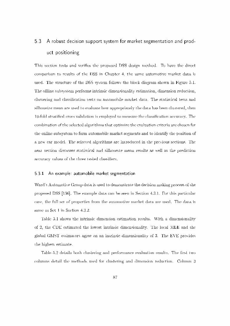
5.3 A robust decision support system for market segmentation and prod-
uct positioning
This section tests and veri�es the proposed DSS design method. To have the direct
comparison to results of the DSS in Chapter 4, the same automotive market data is
used. The structure of the DSS system follows the block diagram shown in Figure 5.1.
The o�ine subsystem performs intrinsic dimensionality estimation, dimension reduction,
clustering and classi�cation tests on automobile market data. The statistical tests and
silhouette mean are used to evaluate how appropriately the data has been clustered, then
10-fold strati�ed cross validation is employed to measure the classi�cation accuracy. The
combination of the selected algorithms that optimize the evaluation criteria are chosen for
the online subsystem to form automobile market segments and to identify the position of
a new car model. The selected algorithms are introduced in the previous sections. The
next section discusses statistical and silhouette mean results as well as the prediction
accuracy values of the three tested classi�ers.
5.3.1 An example: automobile market segmentation
Ward's Automotive Group data is used to demonstrate the decision making process of the
proposed DSS [136]. The example data can be seen in Section 4.3.1. For this particular
case, the full set of properties from the automotive market data are used. The data is
same as Set 1 in Section 4.3.2.
Table 5.1 shows the intrinsic dimension estimation results. With a dimensionality
of 2, the CDE estimated the lowest intrinsic dimensionality. The local MLE and the
global GMST estimators agree on an intrinsic dimensionality of 3. The EVE provides
the highest estimate.
Table 5.2 details both clustering and performance evaluation results. The �rst two
columns detail the methods used for clustering and dimension reduction. Column 3
87

Table 5.1: Intrinsic dimension estimation results.
Method EVE MLE CDE GMST
Dimensions 10 3 2 3
71.38± 32.58GAda
95.78± 5.21NN
99.19± 1.63SVM
40
60
80
100Classi�cation
accuracy
Figure 5.2: Classi�cation accuracy over all clusters.
indicates the intrinsic dimensionality, the numbers are linked to the results shown in Table
5.1. The last column of the clustering part indicates the number of clusters found by the
individual clustering algorithms. The �rst two columns, of the performance evaluation
part, state M and σ of the clusters. The following silhouette mean column provides a
statistical indication of the cluster performance (0 worst, 1 best). The last three columns
of the Table 5.1 provide the 10-fold strati�ed cross validated accuracy results for the
three tested classi�ers. For example, the �rst result row in Table 5.2 indicates that,
with a PCA based dimensionality reduction from 31 to 2 (CDE), the K-means algorithm
partitions the data into 2 clusters. Comparing these clusters results in M = 24.5 and σ
= 152.45. With 0.67 the silhouette mean is high. Therefore, the low accuracy score for
GAda of 25.24% is unexpected. With 99.68% vs. 98.25% the SVM outperforms the NN.
Figure 5.2 shows mean and standard deviation of the classi�cation accuracy over all
analyzed data, i.e. across the respective column in Table 5.2.
88
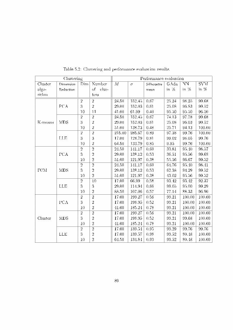
Table 5.2: Clustering and performance evaluation results.
Clustering Performance evaluation
Clusteralgo-rithm
Dimension
Reduction
Dim Numberof clus-ters
M σ Silhouette
mean
GAdain %
NNin %
SVMin %
K-means
PCA2 2 24.50 152.45 0.67 25.24 98.25 99.683 2 29.00 152.03 0.61 25.08 96.83 99.5210 11 41.00 61.99 0.40 95.50 95.50 96.50
MDS2 2 24.50 152.45 0.67 74.13 97.78 99.683 2 29.00 152.03 0.61 25.08 96.03 99.5210 2 51.00 138.73 0.48 25.71 94.13 100.00
LLE2 2 215.00 285.67 0.89 97.38 99.76 100.003 3 17.00 128.79 0.81 99.02 98.05 99.7610 2 64.50 133.79 0.85 0.95 99.76 100.00
FCM
PCA2 2 24.50 141.17 0.60 33.81 95.40 98.573 2 29.00 138.12 0.53 36.51 95.56 99.6810 2 51.00 121.97 0.38 55.56 96.67 99.52
MDS2 2 24.50 141.17 0.60 64.76 95.40 98.413 2 29.00 138.12 0.53 62.38 94.29 99.5210 2 51.00 121.97 0.38 43.02 95.56 99.52
LLE2 10 17.00 66.99 0.58 93.42 93.42 92.373 3 29.00 114.94 0.66 99.05 95.00 99.2910 2 88.50 107.06 0.57 77.14 88.33 96.90
Cluster
PCA2 2 17.00 199.27 0.56 99.21 100.00 100.003 2 17.00 198.95 0.52 99.21 100.00 100.0010 2 41.00 185.24 0.78 99.21 100.00 100.00
MDS2 2 17.00 199.27 0.56 99.21 100.00 100.003 2 17.00 198.95 0.52 99.21 99.68 100.0010 2 41.00 185.24 0.78 99.21 100.00 100.00
LLE2 2 17.00 139.54 0.95 99.29 99.76 99.763 2 17.00 139.57 0.98 99.52 80.48 100.0010 2 64.50 134.84 0.93 99.52 80.48 100.00
89
5.3.2 Lessons learned
The block diagram in Figure 5.1 gives a blueprint on how to construct the o�ine and
online subsystems for a DSS. Initially there is the fundamental split between o�ine and
online subsystems. The construction of the o�ine subsystem is more challenging, because
there is no a priori knowledge on what algorithms to use. This lack of knowledge forces
us to conduct empirical science by trying out di�erent algorithms and measuring their
performance. Therefore, it is important to get an overview of the existing algorithms in
the respective �elds. From an application development point of view it is not feasible
to implement new algorithms, these algorithms have to come from libraries and other
prior implementations. Therefore, the Matlab eco-system is a good starting point for
�nding these algorithm implementations. The subsequent step is crucial: testing these
algorithms. The testing should involve at least two di�erent methods, namely a statistical
method and a classi�cation method. The statistical method ensures that the results are
believable and they show whether or not the investigator is on the right track.
DM algorithms are used to extract market segmentation information from automotive
market data and subsequently machine learning algorithms are used for online decision
support of a new car model positioning. In this particular setup, the market data di-
mensionality is too high, therefore the �rst processing step in the o�ine subsystem is
the intrinsic dimensionality reduction. Four di�erent estimation methods give three dif-
ferent results. The diversity of these results indicates that there is no single objective
method which delivers the correct solution to problems encountered in the construction
of a DSS. Similarly, the three di�erent methods, in the subsequent dimension reduction
step, lead also to di�erent results. The dimension reduction step changes the meaning of
the individual parameters, i.e. after dimension reduction the parameters have no direct
relationship to physical properties, such as Length and Width. Therefore, the subse-
quent clustering and classi�cation steps have to extract meaning from this reduced set of
parameters. As before, there are di�erent clustering algorithms in existence and for this
90
work three of them are tested. As expected, di�erent clustering algorithms give di�erent
results.
For this case study, the result of the clustering algorithms is interpreted as market
segmentation information. In other words, this clustering function maps individual car
models to di�erent market segments. As part of the o�ine subsystem, 36 di�erent
clustering results are observed, each of which are obtained with a di�erent algorithm
con�guration. The last step in the o�ine subsystem is concerned with the task of �nding
the best algorithm combination. This step is crucial, therefore the vigorous evaluations
are conducted on the clustering information in terms ofM , σ, silhouette mean and the 10-
fold strati�ed cross validated accuracy of three di�erent classi�cation algorithms. M and
σ are straight forward statistical methods to compare the clustering results. A M close
to the mean and a low standard deviation indicate clusters of similar size. For example,
with σ=61.99, K-means clustering on a PCA reduced 10 dimensional dataset achieved
the lowest standard-deviation, i.e. the cluster size is similar. The high silhouette of 0.95
mean is obtained with the cluster algorithm acting on LLE reduced data. However, these
statistical methods do not correlate well with the classi�cation results.
Using classi�cation algorithms to evaluate the performance of the market segmenta-
tion has a dual purpose. The 10-fold strati�ed cross validation test is the best practical
test, because it is speci�cally targeted to the problem of �nding the market segment for
a new product from its properties. The most accurate classi�cation algorithm will serve
in the online subsystem to provide decision support. There is a number of clustering
strategies which leads to high and highest classi�cation accuracy. Therefore, the cluster-
ing method can be selected according to secondary considerations, such as the number
of clusters and the cluster homogeneity. For example, if chose silhouette mean and pre-
diction accuracy as performance criteria, the following combination should be chosen for
the online subsystem to provide decision support: MLE or GMST for intrinsic dimension
estimation which gives 3 dimension estimation, the LLE for dimension reduction, the
91
Cluster for clustering and SVM for classi�cation. This combination yields the highest
silhouette mean of 0.98 and highest prediction accuracy of 100% as shown in Table 5.2.
As shown in Figure 5.2, with the lowest mean of 71.38% and highest variance of
32.58%, the GAda classi�er performs worst among three. On the contrary, for this
particular case data used, it is found out that the SVM algorithm scores consistently
well. Figure 5.2 indicates that, on average, it outperforms NN and GAda with the
highest mean of 99.19% and smallest variance 1.63%. Therefore, the online subsystem
features the SVM algorithm for decision support.
Looking back to the results from table 4.2 in Section 4.3.2, both the silhouette mean
of 0.40 and prediction accuracy of 76.4% of the previous DSS are quite low. Which
means that the combination of the PCA, K-means, and GAda isn't a good choice for
this particular data set. This result is consistent with the result in Table 5.2. However,
as discussed in Section 4.3.2, when the dimension of the chosen data set varies, both the
clustering results and DSS performances vary dramatically. With the full set of design
parameters (31 parameters), Table 5.2 shows that the majority of the chosen methods
yield clustering results of two, and a few methods yield clustering results of three, ten
and eleven. Based on these objective results, a decision maker might raise a question:
�How can two clusters of these 639 cars be helpful?�. There are merits in asking how
helpful an objective measure is. A question like �what if we chose more representative
design parameters in the data set?� can be formulated and incorporated in the DSS. As
we discussed in Section 4.3.3, in the �what if� scenarios where di�erent design parameter
are chosen, the DSS will yield di�erent market segmentation and product positioning
results. Through examination of di�erent results and current product portfolios, the
decision makers can create a justi�cation for developing new products. If a particular
objective measure is not helpful, we have to look for di�erent or more suitable objective
measures to increase their relevance. In general, it is not a good idea to dismiss an
objective measure, because it fails a subjective test. Failing that test is a motivation
92
which generates tasks for future work.
5.4 Summary and preview
This chapter delivers a blueprint on how to construct o�ine and online subsystems of
a DSS for market segmentation and product positioning. The o�ine system uses DM
techniques to extract useful information from the available data. In general, it is di�cult
to know a priori what are the best algorithms for information extraction, because of the
fuzzy relationship between data and clusters. Therefore, empirical science is needed to
�nd the best combination from an available set of algorithms. The online subsystem de-
livers active decisions that can help during the decision making process. To demonstrate
the empirical process is demonstrated based on data from the US automotive market,
which leads to the selection of the best processing structure with the most suitable algo-
rithms. Four intrinsic dimensionality estimation algorithms are used on the data. These
algorithms provided three di�erent estimates (2, 3, 10) which are used in the dimen-
sionality reduction step. To be speci�c, three di�erent dimension reduction algorithms
are employed to compress the original data into the prior evaluated dimensions. The
resulting nine datasets are fed into three di�erent clustering algorithms. The results of
these clustering algorithms are analyzed with statistical methods, silhouette mean and
three classi�cation algorithms. The main �nding of the analysis step is that the SVM
classi�cation algorithm outperforms both NN and GAda. Therefore, the SVM classi�er
is best matched for this type of data, hence it should be used in the online subsystem.
The analysis results show that empirical science is necessary to �nd the best combi-
nation of algorithms for the problem at hand. Furthermore, there is even some leverage
to adjust speci�c parameters and conduct a `What if' analysis as shown in Scenario 3 in
Section 4.3.2. The most important point is to assess the algorithm combination quality
with di�erent test methods, such as statistical evaluation and classi�cation tests. These
93
test results have to guide the empirical process to select the most suitable algorithms.
After the intense study of algorithm structures and outlining the merits of o�ine and
online systems, we are in a position to answer the questions posed in Section 4.3.3:
� Is the combination of the PCA, K-means and GAda algorithms the best way to
form the DSS? Would an alternative DSS design yield higher prediction accuracy?
It turns out that the arbitrary selection in the previous DSS is not a wise choice.
The GAda prediction accuracy is pretty disappointing, as discussed in Section 5.3.2.
Thus, the poor accuracy of the randomly chosen algorithm validates the main point
of this chapter: rigorous testing should be conducted in the o�ine subsystem, and
only the best algorithms are chosen for the online subsystem to provide reliable
decision support.
� What will be the more robust and reliable way to construct a data-driven DSS for
market segmentation and product positioning? As shown in Figure 3.2, the pro-
posed method partitioned the DSS into four subsystems. Each of these subsystems
has its own functions and is realized using di�erent tools and techniques. The data
subsystem provides e�cient data storage and easy retrieval for large volumes and
high dimensional data. It serves as a basis for the DSS. The o�ine subsystem
employs vigorous evaluation methods to �nd the best combination of DM and ma-
chine learning algorithms. Only the algorithm combination that yields the highest
classi�cation accuracy is used in the online subsystem to provide reliable decision
support through a user friendly Graphical User Interface (GUI).
With the focus on data-driven market segmentation and product positioning methods,
Chapters 4 and 5 illustrated how to construct a robust DSS, along with a review and
comparison of the most commonly used DM and machine learning techniques. Chapters
6 and 7 move one step forwards using Additive Manufacturing (AM) technologies and
providing improved customization for product family designs.
94
Chapter 6
Product family design for additive
manufacturing
This chapter presents an Additive Manufacturing (AM) process model for product fam-
ily design. As discussed in Section 2.4, AM is projected to have a profound impact on
the mass customization of consumer products. In order to take advantage of this man-
ufacturing resource, new design methods have to be established. The need is addressed
by proposing an AM centered process model for product family design. The proposed
model re�ects the ability of AM to produce arbitrarily complex structures with virtually
no tooling e�ort, and it makes these powerful properties available to practitioners work-
ing in the �eld of product family design. By utilizing AM, all constraints, which arise in
conventional product family designs, from �nding a compromise between commonality
and product performance are eliminated.
This chapter is organized as follows: Section 6.1 presents a brief review on the in-
�uences of AM on product family design. Section 6.2 introduces the methods which
are used to realize the proposed process model. Section 6.3 introduces a case study to
test the proposed model. Section 6.4 summarizes the virtuous of AM for product family
design.
95

6.1 Overview of in�uences of additive manufacturing to product family
design
Competition in the global market place lead to the advancement of platform-based prod-
uct families during the early 1980s. The product family paradigm introduces product
proliferation while taking advantage of mass production e�ciency [7]. Many companies
invest in product family development practices so that they can provide su�cient variety
to the market while maintaining the economies of scale and scope within their manufac-
turing capabilities [8]. Conventional product family optimization focuses on exploiting
the commonality between individual products [15]. The fundamental assumption is that
common components are less cost intensive than distinctive ones [168]. Hence, a prereq-
uisite to harvest the bene�ts of product family design is process planning, with a special
focus on keeping the production process as stable as possible [169]. In accordance with
the diversity required by customized products, process family planning involves large data
volumes pertaining to both the product family and the process family to be planned [170].
In addition, process family planning requires complex considerations which take into ac-
count marketing information and manufacturing restrictions, such as limited resources
existing on shop �oors [171]. Thus, a fundamental issue in process family planning is the
modeling of production processes [92].
A production process describes routings, operations and manufacturing resources
(e.g., machines, tools, �xtures and jigs) that are adopted to materialize a design [172].
From the production process perspective, Additive Manufacturing (AM) is a manufactur-
ing resource that produces shaped parts by gradual creation or addition of solid material.
This is fundamentally di�erent from traditional forming and material removal manufac-
turing techniques [173]. The main bene�t of AM is the ability to manufacture parts of
virtually any geometric complexity without the need for tooling [174]. The Economist
predicts that these bene�cial properties have a profound impact on the way manufac-
96

turing businesses operate and indeed on how they generate revenue [175]. For product
family design, AM is used to add value by customizing selected features [80]. Hague et
al. [88] predicted that AM will have a profound in�uence on the product family pro-
duction process. Hence, AM requires new design concepts and models [174, 176]. These
concepts should exploit the �exibilities, o�ered by the AM, in an optimal way [177]. To
achieve customization through AM requires that we update or indeed upgrade the design
methods in such a way that a practitioner can translate these �exibilities into tangible
advantages in the global market place.
This chapter addresses the need to model AM as part of a product family design
process. It's recognized that the unique properties of AM will fundamentally alter con-
siderations about commonality, customization and ultimately pro�tability. This chapter
highlights the opportunities for AM based product family design to operate in a much
broader design space that is free from constraints which arise in conventional product
family designs from �nding a compromise between commonality and performance. To
translate the bene�ts of AM into customization and cost reduction, a novel product fam-
ily design model is proposed. The model allows practitioners to evaluate the performance
of an in�nite number of product designs and select the most suitable ones. To be speci�c,
topology optimization and Finite Element Analysis (FEA) are used to generate a per-
formance graph for individual component groups. The performance graph is combined
with the result of a cost model. Therefore, the manufacturing cost is related to the prod-
uct performance. Having such a clear relationship opens up a fair competition between
individual component realizations and the most suitable product family design can be
selected. To verify the proposed model, a case study was conducted and the customized
product family designs were fabricated with Fused Deposition Modeling (FDM). The
results of the case study con�rm the �tnesses of the proposed model.
97

6.2 An additive manufacturing process model for product family design
This section introduces the AM process model for product family design, along with a
formulation for a scalable product family design problem. AM is used for mechanical part
fabrication. Figure 6.1 shows a block diagram of the proposed model. The model starts
with the designer de�ning the primary requirements and constraints that will de�ne the
product family. In the second step, topology optimization is used to generate optimal
individual designs to best achieve the design requirements. In a subsequent step, the
performance and the cost measures are investigated. FEA is employed to verify the
ful�llment of the performance requirements. The AM cost analysis allows us to identify
potential commonalities in order to reduce the product family development cost further.
If the requirement check is failed, the design process goes back to the �rst step. Once
the requirements are fully ful�lled and the cost is further reduced, a customized product
family is accomplished. AM is used to realize the customized designs and mechanical
veri�cation is carried out. The test results are compared with FEA simulation results.
6.2.1 Product family design
The proposed model incorporates AM technologies into the design of a scalable product
family. The idea of the scalable product family is that the platform is adjustable by
changing values of dimensions or other parameters to adjust the sizes of components in
the platform. This is in contrast to modular product families or platforms where modules
are swapped in order to generate variety.
The processes basis is the identi�cation of the product family design and Design for
Additive Manufacturing (DFAM) requirements and constraints, which have to be met to
ful�ll the product functionalities. The requirements also represent the objectives needed
for the de�nition of the topology optimization process.
98
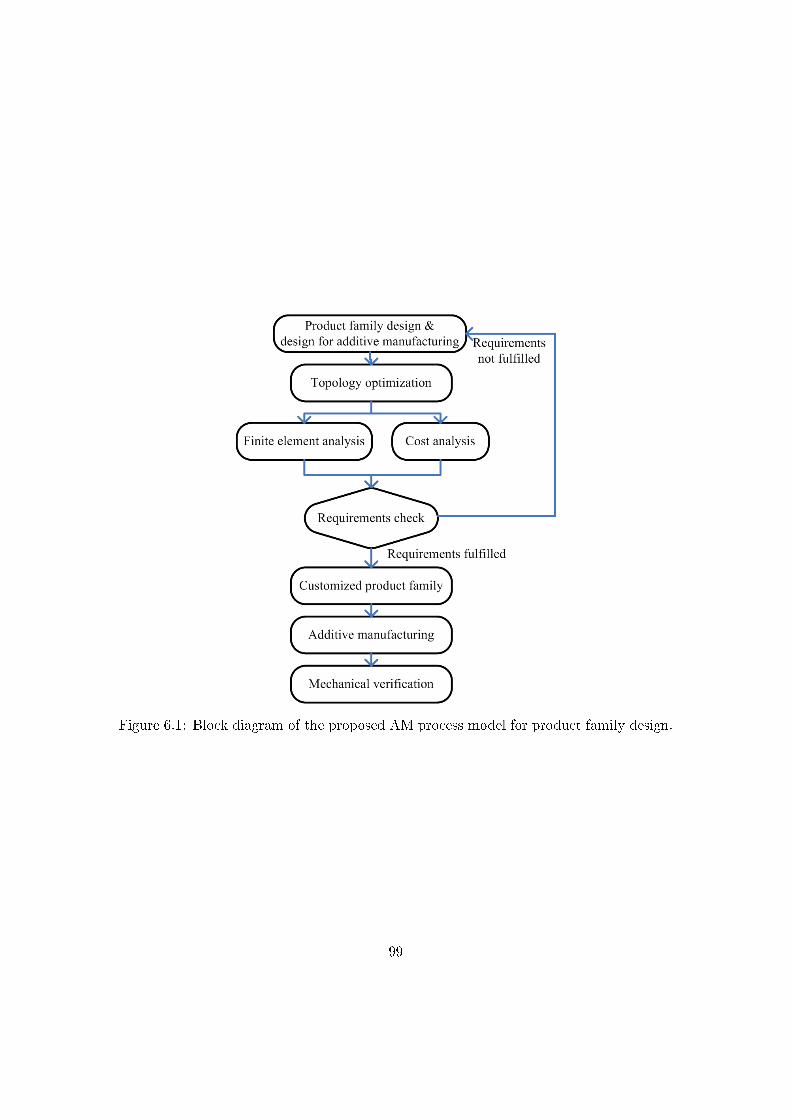
Figure 6.1: Block diagram of the proposed AM process model for product family design.
99
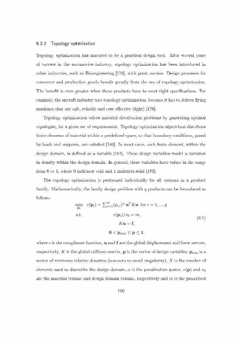
6.2.2 Topology optimization
Topology optimization has matured to be a practical design tool. After several years
of success in the automotive industry, topology optimization has been introduced in
other industries, such as Bioengineering [178], with great success. Design processes for
consumer and production goods bene�t greatly from the use of topology optimization.
The bene�t is even greater when these products have to meet tight speci�cations. For
example, the aircraft industry uses topology optimization, because it has to deliver �ying
machines that are safe, reliable and cost e�ective (light) [179].
Topology optimization solves material distribution problems by generating optimal
topologies, for a given set of requirements. Topology optimization algorithms distribute
�nite elements of material within a prede�ned space, so that boundary conditions, posed
by loads and supports, are satis�ed [180]. In most cases, each �nite element, within the
design domain, is de�ned as a variable [181]. These design variables model a variation
in density within the design domain. In general, these variables have values in the range
from 0 to 1, where 0 indicates void and 1 indicates solid [182].
The topology optimization is performed individually for all variants in a product
family. Mathematically, the family design problem with q products can be formulated as
follows:
minpi
c(pi) =∑N
c=1(pi,c)α uTKu for i = 1, ..., q
s.t. v(pi)/v0 = m,
Ku = f ,
0 < pmin ≤ p ≤ 1.
(6.1)
where c is the compliance function, u and f are the global displacement and force vectors,
respectively, K is the global sti�ness matrix, p is the vector of design variables, pmin is a
vector of minimum relative densities (non-zero to avoid singularity), N is the number of
elements used to discretize the design domain, α is the penalization power, v(p) and v0
are the material volume and design domain volume, respectively and m is the prescribed
100
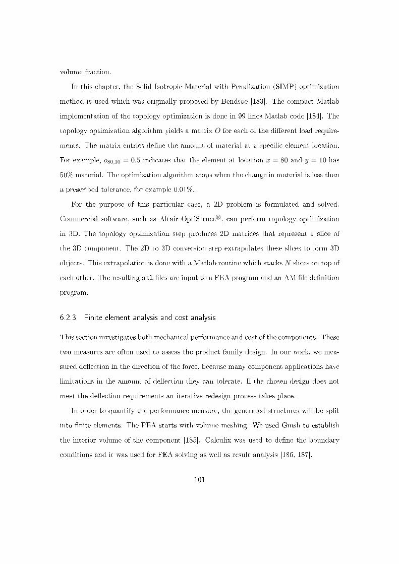
volume fraction.
In this chapter, the Solid Isotropic Material with Penalization (SIMP) optimization
method is used which was originally proposed by Bendsøe [183]. The compact Matlab
implementation of the topology optimization is done in 99 lines Matlab code [184]. The
topology optimization algorithm yields a matrix O for each of the di�erent load require-
ments. The matrix entries de�ne the amount of material at a speci�c element location.
For example, o80,10 = 0.5 indicates that the element at location x = 80 and y = 10 has
50% material. The optimization algorithm stops when the change in material is less than
a prescribed tolerance, for example 0.01%.
For the purpose of this particular case, a 2D problem is formulated and solved.
Commercial software, such as Altair OptiStructr, can perform topology optimization
in 3D. The topology optimization step produces 2D matrices that represent a slice of
the 3D component. The 2D to 3D conversion step extrapolates these slices to form 3D
objects. This extrapolation is done with a Matlab routine which stacks N slices on top of
each other. The resulting stl �les are input to a FEA program and an AM �le de�nition
program.
6.2.3 Finite element analysis and cost analysis
This section investigates both mechanical performance and cost of the components. These
two measures are often used to assess the product family design. In our work, we mea-
sured de�ection in the direction of the force, because many component applications have
limitations in the amount of de�ection they can tolerate. If the chosen design does not
meet the de�ection requirements an iterative redesign process takes place.
In order to quantify the performance measure, the generated structures will be split
into �nite elements. The FEA starts with volume meshing. We used Gmsh to establish
the interior volume of the component [185]. Calculix was used to de�ne the boundary
conditions and it was used for FEA solving as well as result analysis [186, 187].
101
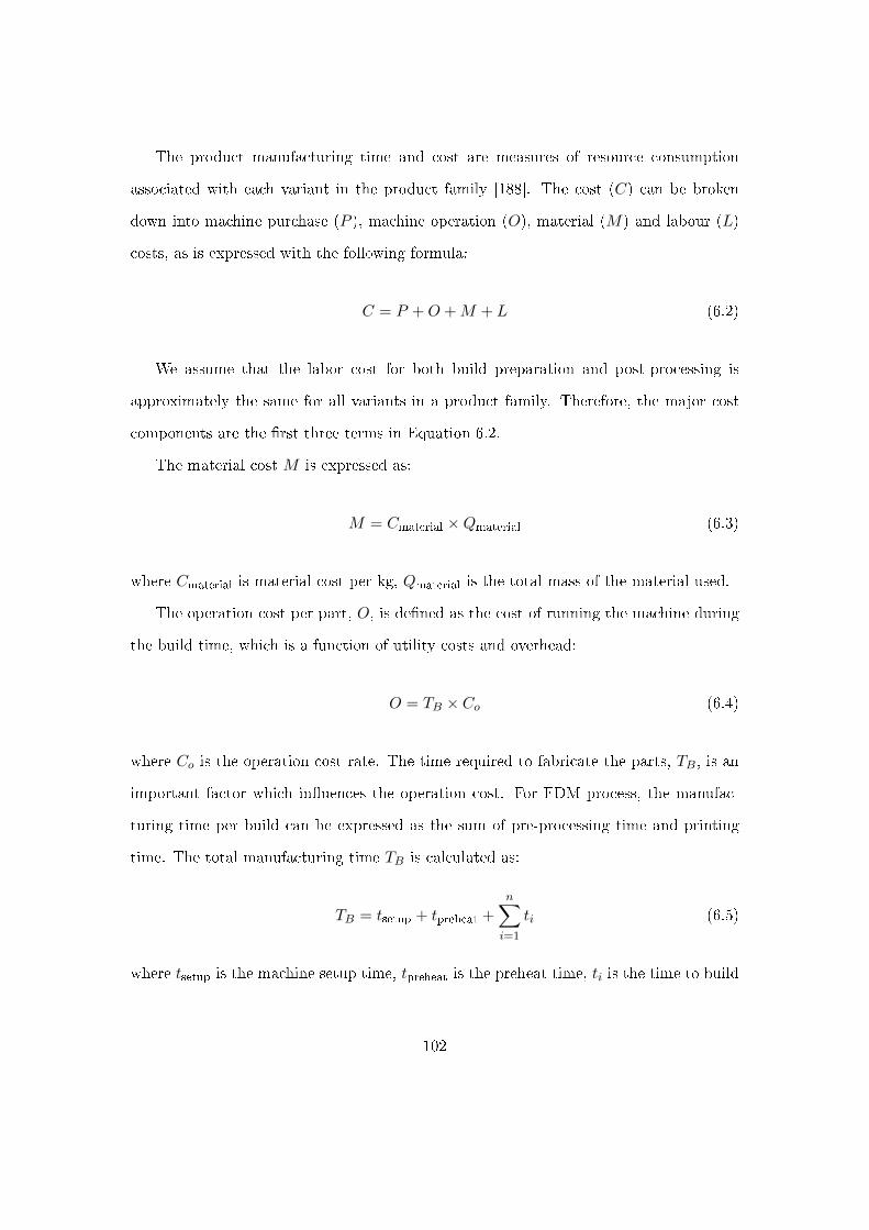
The product manufacturing time and cost are measures of resource consumption
associated with each variant in the product family [188]. The cost (C) can be broken
down into machine purchase (P ), machine operation (O), material (M) and labour (L)
costs, as is expressed with the following formula:
C = P +O +M + L (6.2)
We assume that the labor cost for both build preparation and post-processing is
approximately the same for all variants in a product family. Therefore, the major cost
components are the �rst three terms in Equation 6.2.
The material cost M is expressed as:
M = Cmaterial ×Qmaterial (6.3)
where Cmaterial is material cost per kg, Qmaterial is the total mass of the material used.
The operation cost per part, O, is de�ned as the cost of running the machine during
the build time, which is a function of utility costs and overhead:
O = TB × Co (6.4)
where Co is the operation cost rate. The time required to fabricate the parts, TB, is an
important factor which in�uences the operation cost. For FDM process, the manufac-
turing time per build can be expressed as the sum of pre-processing time and printing
time. The total manufacturing time TB is calculated as:
TB = tsetup + tpreheat +
n∑i=1
ti (6.5)
where tsetup is the machine setup time, tpreheat is the preheat time, ti is the time to build
102
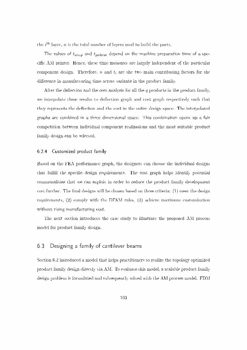
the ith layer, n is the total number of layers used to build the parts.
The values of tsetup and tpreheat depend on the machine preparation time of a spe-
ci�c AM printer. Hence, these time measures are largely independent of the particular
component design. Therefore, n and ti are the two main contributing factors for the
di�erence in manufacturing time across variants in the product family.
After the de�ection and the cost analysis for all the q products in the product family,
we interpolate these results to de�ection graph and cost graph respectively such that
they represents the de�ection and the cost in the entire design space. The interpolated
graphs are combined in a three dimensional space. This combination opens up a fair
competition between individual component realizations and the most suitable product
family design can be selected.
6.2.4 Customized product family
Based on the FEA performance graph, the designers can choose the individual designs
that ful�ll the speci�c design requirements. The cost graph helps identify potential
commonalities that we can exploit in order to reduce the product family development
cost further. The �nal designs will be chosen based on three criteria: (1) meet the design
requirements, (2) comply with the DFAM rules, (3) achieve maximum customization
without rising manufacturing cost.
The next section introduces the case study to illustrate the proposed AM process
model for product family design.
6.3 Designing a family of cantilever beams
Section 6.2 introduced a model that helps practitioners to realize the topology optimized
product family design directly via AM. To evaluate this model, a scalable product family
design problem is formulated and subsequently solved with the AM process model. FDM
103
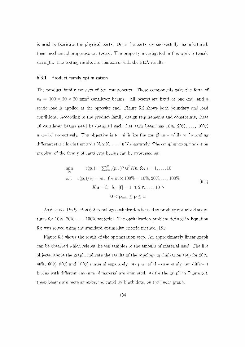
is used to fabricate the physical parts. Once the parts are successfully manufactured,
their mechanical properties are tested. The property investigated in this work is tensile
strength. The testing results are compared with the FEA results.
6.3.1 Product family optimization
The product family consists of ten components. These components take the form of
v0 = 100 × 20 × 20 mm3 cantilever beams. All beams are �xed at one end, and a
static load is applied at the opposite end. Figure 6.2 shows both boundary and load
conditions. According to the product family design requirements and constraints, these
10 cantilever beams need be designed such that each beam has 10%, 20%, . . . , 100%
material respectively. The objective is to minimize the compliance while withstanding
di�erent static loads that are 1 N, 2 N, . . . , 10 N separately. The compliance optimization
problem of the family of cantilever beams can be expressed as:
minpi
c(pi) =∑N
c=1(pi,c)α uTKu for i = 1, . . . , 10
s.t. v(pi)/v0 = m, for m× 100% = 10%, 20%, . . . , 100%
Ku = f , for |f | = 1 N, 2 N, . . . , 10 N
0 < pmin ≤ p ≤ 1.
(6.6)
As discussed in Section 6.2, topology optimization is used to produce optimized struc-
tures for 10%, 20%, . . . , 100% material. The optimization problem de�ned in Equation
6.6 was solved using the standard optimality criteria method [181].
Figure 6.3 shows the result of the optimization step. An approximately linear graph
can be observed which relates the ten samples to the amount of material used. The �ve
objects, above the graph, indicate the results of the topology optimization step for 20%,
40%, 60%, 80% and 100% material separately. As part of the case study, ten di�erent
beams with di�erent amounts of material are simulated. As for the graph in Figure 6.3,
these beams are mere samples, indicated by black dots, on the linear graph.
104
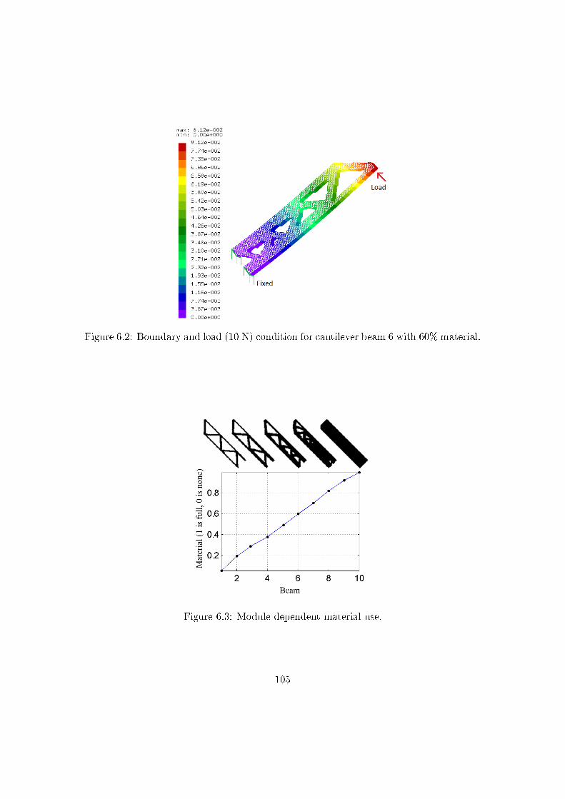
Figure 6.2: Boundary and load (10 N) condition for cantilever beam 6 with 60% material.
Figure 6.3: Module dependent material use.
105
6.3.2 Finite element analysis and performance surfaces
The FEA step analyzes both de�ection and stress for each beam with static loads of
1 N, 2 N, . . . , 10 N. The results constituted 100 (number of structures × number of
load scenarios) samples in 3-dimensional de�ection and stress spaces. In an interpolation
step, we connected these samples and thereby we created performance surfaces. These
performance surfaces have an in�nite number of points, therefore it is possible to assess
an in�nite number of components. Within this in�nite pool of possible components, there
is one component which meets the design requirements, in terms of de�ection and stress.
Hence, the designers can select an optimal component design based on a prescribed set
of performance criteria.
Figure 6.4 shows the de�ection performance surface. The intersection between two
black lines indicates a sample point. For example, through FEA we found that Beam
1 (10% v0) shows a maximum de�ection of 0.025 mm and Beam 10 (100% v0) shows a
de�ection of just 0.01 mm. The surface facets of the de�ection performance surface are
interpolated. To be speci�c, they describe an operation which maps a beam, with any
amount of material which is subjected to a load scenario from 1 N to 10 N, to a speci�c
de�ection. This straight forward interpolation was possible, because the performance
surface is well behaved, i.e. it behaves according to expectations. For example, the
beam with only 10% material has the highest de�ection and a full beam shows the least
de�ection. There is a linear relationship between de�ection and load for all the beams.
The relationship between di�erent beams (with di�erent amounts of material) having the
same load can be approximated by an exponential decay function.
Figure 6.5 shows the stress performance surface. This performance surface is not well
behaved, because, contrary to our expectation, the stress in the material does not depend
on the amount of material used to construct the beam. The beam with 90% material
shows the second highest stress levels for all the load conditions. Furthermore, the beam
with 40% material shows higher stress levels than the beam with 30% material. Upon
106
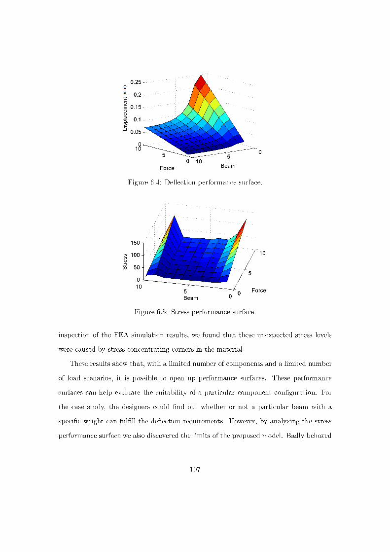
Figure 6.4: De�ection performance surface.
Figure 6.5: Stress performance surface.
inspection of the FEA simulation results, we found that these unexpected stress levels
were caused by stress concentrating corners in the material.
These results show that, with a limited number of components and a limited number
of load scenarios, it is possible to open up performance surfaces. These performance
surfaces can help evaluate the suitability of a particular component con�guration. For
the case study, the designers could �nd out whether or not a particular beam with a
speci�c weight can ful�ll the de�ection requirements. However, by analyzing the stress
performance surface we also discovered the limits of the proposed model. Badly behaved
107
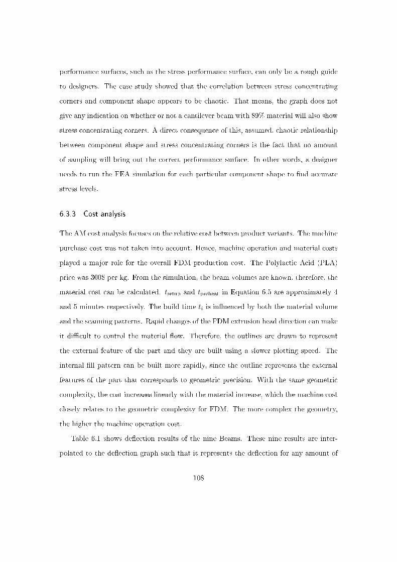
performance surfaces, such as the stress performance surface, can only be a rough guide
to designers. The case study showed that the correlation between stress concentrating
corners and component shape appears to be chaotic. That means, the graph does not
give any indication on whether or not a cantilever beam with 89% material will also show
stress concentrating corners. A direct consequence of this, assumed, chaotic relationship
between component shape and stress concentrating corners is the fact that no amount
of sampling will bring out the correct performance surface. In other words, a designer
needs to run the FEA simulation for each particular component shape to �nd accurate
stress levels.
6.3.3 Cost analysis
The AM cost analysis focuses on the relative cost between product variants. The machine
purchase cost was not taken into account. Hence, machine operation and material costs
played a major role for the overall FDM production cost. The Polylactic Acid (PLA)
price was 300$ per kg. From the simulation, the beam volumes are known, therefore, the
material cost can be calculated. tsetup and tpreheat in Equation 6.5 are approximately 4
and 5 minutes respectively. The build time ti is in�uenced by both the material volume
and the scanning patterns. Rapid changes of the FDM extrusion head direction can make
it di�cult to control the material �ow. Therefore, the outlines are drawn to represent
the external feature of the part and they are built using a slower plotting speed. The
internal �ll pattern can be built more rapidly, since the outline represents the external
features of the part that corresponds to geometric precision. With the same geometric
complexity, the cost increases linearly with the material increase, which the machine cost
closely relates to the geometric complexity for FDM. The more complex the geometry,
the higher the machine operation cost.
Table 6.1 shows de�ection results of the nine Beams. These nine results are inter-
polated to the de�ection graph such that it represents the de�ection for any amount of
108
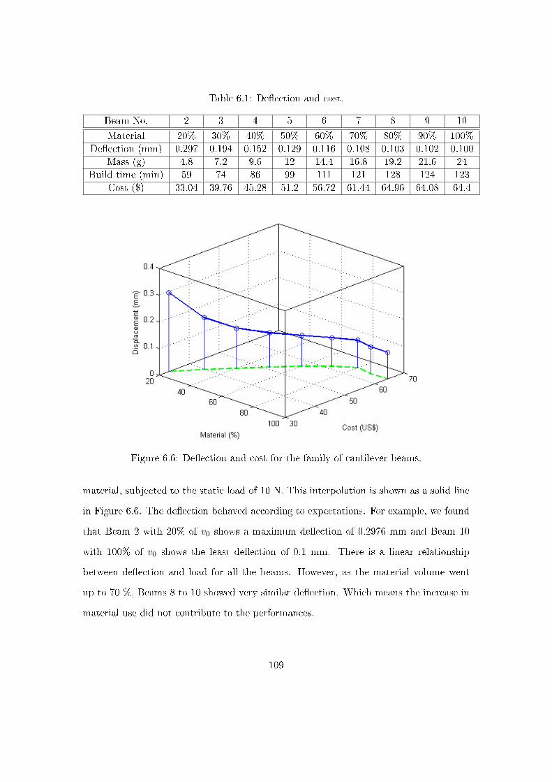
Table 6.1: De�ection and cost.
Beam No. 2 3 4 5 6 7 8 9 10
Material 20% 30% 40% 50% 60% 70% 80% 90% 100%
De�ection (mm) 0.297 0.194 0.152 0.129 0.116 0.108 0.103 0.102 0.100
Mass (g) 4.8 7.2 9.6 12 14.4 16.8 19.2 21.6 24
Build time (min) 59 74 86 99 111 121 128 124 123
Cost ($) 33.04 39.76 45.28 51.2 56.72 61.44 64.96 64.08 64.4
Figure 6.6: De�ection and cost for the family of cantilever beams.
material, subjected to the static load of 10 N. This interpolation is shown as a solid line
in Figure 6.6. The de�ection behaved according to expectations. For example, we found
that Beam 2 with 20% of v0 shows a maximum de�ection of 0.2976 mm and Beam 10
with 100% of v0 shows the least de�ection of 0.1 mm. There is a linear relationship
between de�ection and load for all the beams. However, as the material volume went
up to 70 %, Beams 8 to 10 showed very similar de�ection. Which means the increase in
material use did not contribute to the performances.
109
The build time ti was obtained from the open source software Cura1. The estimation
of the build time and cost of the product family components are listed in Table 6.1. The
costs for Beams 2 to 10 were interpolated to cost graph that is shown as a dashed line
in Figure 6.6. We observed that from Beams 2 to 8 both the build time and the cost
increased. However, the build time and cost of Beams 9 and 10 decreased even with
more material. From Beams 2 to 10, the material volume increase linearly. Beams 2
to 4 have similar geometric complexity. From Beams 5 to 7, the geometric complexity
increases that results in longer scanning length and frequent direction changes of the
extrusion head. From Beams 8 to 10, the geometric complexity decreases that results in
short scanning length. This explain the cost drop for Beams 9 and 10.
The above discussion was based on the FDM process. For di�erent AM processes, the
cost pro�les di�er. For example, in 3D printing, the bulk of each printed layer, regardless
of complexity, is deposited by the same and rapid spreading process. Therefore the build
time will be a constant for Beams 1 to 10.
6.3.4 Customization of the cantilever beam product family
The results from the previous step indicated that, though AM o�ers freedom of design,
it does not always o�er complexity for free. Speci�cally, for processes, such as jetting-
based systems, the �complexity is free� statement is true; conversely it is not correct
for extrusion-based systems [79], such as FDM. The build times are higher for complex
shapes than for simple shapes since the extrusion-based processes have to trace out the
the cross section pro�le.
Following the updated design requirements, Beams 1 and 2 share the same design
(20% v0) to comply with DFAM restriction of minimum wall thickness, Beams 3, 4, 5,
6, 7 each have distinct optimal designs that o�er the individualization, Beams 8, 9 and
10 share the same design (100% v0) to reduce the product family cost further without
1http://software.ultimaker.com
110
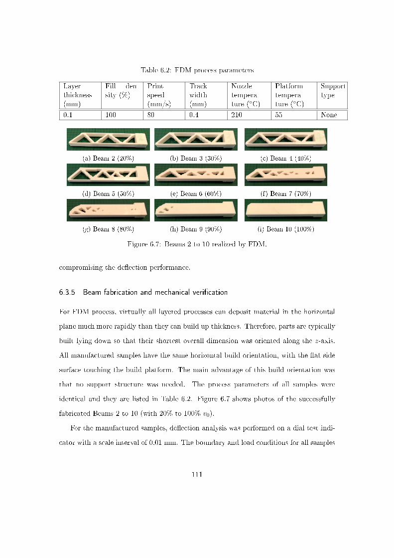
Table 6.2: FDM process parameters
Layerthickness(mm)
Fill den-sity (%)
Printspeed(mm/s)
Trackwidth(mm)
Nozzletempera-ture (◦C)
Platformtempera-ture (◦C)
Supporttype
0.1 100 80 0.4 210 55 None
(a) Beam 2 (20%) (b) Beam 3 (30%) (c) Beam 4 (40%)
(d) Beam 5 (50%) (e) Beam 6 (60%) (f) Beam 7 (70%)
(g) Beam 8 (80%) (h) Beam 9 (90%) (i) Beam 10 (100%)
Figure 6.7: Beams 2 to 10 realized by FDM.
compromising the de�ection performance.
6.3.5 Beam fabrication and mechanical veri�cation
For FDM process, virtually all layered processes can deposit material in the horizontal
plane much more rapidly than they can build up thickness. Therefore, parts are typically
built lying down so that their shortest overall dimension was oriented along the z-axis.
All manufactured samples have the same horizontal build orientation, with the �at side
surface touching the build platform. The main advantage of this build orientation was
that no support structure was needed. The process parameters of all samples were
identical and they are listed in Table 6.2. Figure 6.7 shows photos of the successfully
fabricated Beams 2 to 10 (with 20% to 100% v0).
For the manufactured samples, de�ection analysis was performed on a dial test indi-
cator with a scale interval of 0.01 mm. The boundary and load conditions for all samples
111
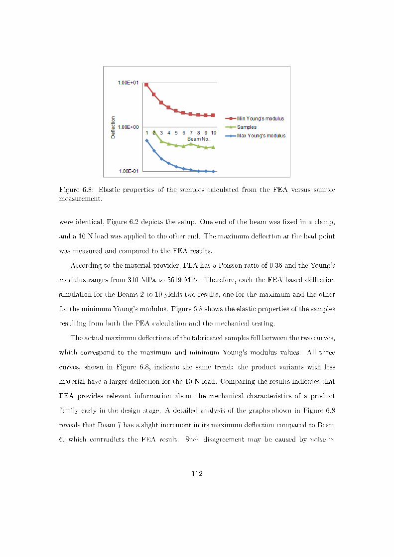
Figure 6.8: Elastic properties of the samples calculated from the FEA versus samplemeasurement.
were identical, Figure 6.2 depicts the setup. One end of the beam was �xed in a clamp,
and a 10 N load was applied to the other end. The maximum de�ection at the load point
was measured and compared to the FEA results.
According to the material provider, PLA has a Poisson ratio of 0.36 and the Young's
modulus ranges from 310 MPa to 5619 MPa. Therefore, each the FEA based de�ection
simulation for the Beams 2 to 10 yields two results, one for the maximum and the other
for the minimum Young's modulus. Figure 6.8 shows the elastic properties of the samples
resulting from both the FEA calculation and the mechanical testing.
The actual maximum de�ections of the fabricated samples fell between the two curves,
which correspond to the maximum and minimum Young's modulus values. All three
curves, shown in Figure 6.8, indicate the same trend: the product variants with less
material have a larger de�ection for the 10 N load. Comparing the results indicates that
FEA provides relevant information about the mechanical characteristics of a product
family early in the design stage. A detailed analysis of the graphs shown in Figure 6.8
reveals that Beam 7 has a slight increment in its maximum de�ection compared to Beam
6, which contradicts the FEA result. Such disagreement may be caused by noise in
112

either the manufacturing process or in the de�ection measurement process. However, the
disagreement was small, therefore it did not a�ect decisions based on FEA models.
6.4 Summary and preview
This chapter proposes an AM process model for product family design. The model out-
lines an optimal customized designs which fully bene�ts from advanced AM technologies.
To substantiate and discuss the proposed model, a case study of designing a family of
10 cantilever beams was introduced. These beams shared the same design space, but
they had di�erent load and weight requirements. Based on these requirements, the
beam realization was broken down to a material distribution problem which was solved
with topology optimization. The optimization process resolved the geometry and the
structural response, such that the optimized designs could be used for AM. The beam
performance was evaluated with FEA and performance surfaces were constructed. These
performance surfaces and the AM cost model helped us to �nd the trade-o� between
performance and cost within the family of products. Subsequently, beam designs were
fabricated using FDM with PLA. The elastic properties of each sample were established
through FEA and measurements. The model validation was done by comparing the
results of both methods.
Compared with existing methods of designing commonality in product families, the
proposed model greatly increased customization by introducing AM resources. Further-
more, a limited number of variants was extrapolated to a performance surface. In the case
study, ten beams and ten load conditions for each beam were used to evaluate an in�nite
number of component realizations. This approach yields a powerful model that can be
used to �nd optimal designs that meet a prescribed set of performance targets. However,
this extrapolation is only valid for well-behaved component properties. In the cantilever
beam case study, the de�ection is such a well behaved linear relationship. In contrast,
113
the levels of stress do not correlate with the amount of material used. To be speci�c,
we found that a beam with 90% material has a stress concentrating corner. Therefore,
this beam showed the second highest levels of stress. Even by taking the restrictions into
account, the proposed model can help practitioners to select optimal components for a
given set of requirements.
The importance of the AM resources will rise as the production costs go down. There-
fore, it will become more and more important to harvest the bene�ts of this production
process in an optimal way. Modeling is a �rst step to address this problem, because it
allows us to conduct `what if' analysis and to extrapolate results. Both considerations are
of eminent importance to change the paradigm for truly individualized product family
development.
The chapter illustrates a simple product family design. More sophisticated product
family design problems are formulated in Chapter 7. As for the cost analysis, we consid-
ered only one component per build in this case study. The e�cient parallel production
of a mixed family of products is demonstrated in next chapter in which the cost saving
of the AM will be even more signi�cant compared to traditional manufacturing methods.
114

Chapter 7
Data-driven product family design for
additive manufacturing: design of a �nger
pump family
In this chapter, the data-driven product family design for Additive Manufacturing (AM)
method, that is proposed in Chapter 3, is applied in full to a dialysis �nger pump family
design for a �nal veri�cation of the proposed method. Details of the market segmentation
and product positioning step have been elaborated in Chapters 4 and 5. In Chapter 6,
the design model that integrates AM into product family design is developed to facilitate
customization.
The arrangements of the chapter is as follows. Section 7.1 presents overview and
motivation of the dialysis pump design. Section 7.2.2 describes Step 1 of the proposed
method, namely market segmentation. In Section 7.2.3, AM technologies are assumed to
enable the customization. Furthermore, a detailed cost model based on Selective Laser
Sintering (SLS) is developed to assess the customization cost. A Utility-Based Compro-
mise Decision Support Problem (u-cDSP) for the family of �nger pump is formulated
115
and solved in Sections 7.2.4 and 7.2.5 respectively. The results are discussed and bench-
marked in Section 7.3. Research �ndings and lessons learned are summarized at the end
of the chapter.
7.1 Overview of the dialysis pump design problem
End Stage Renal Disease (ESRD), commonly known as kidney failure, is a signi�cant
medical problem [189]. With a continuing year-to-year increase over a quarter-century,
more than 738,000 patients were diagnosed with ESRD in 2012 [190]. Over 560,000
patients depend on treatments in dedicated dialysis centres for three to �ve hours, usually
three times a week. Even with dialysis treatment, patients still su�er from accelerated
cardiovascular disease and infections. Hence, technology to miniaturize and automate
home dialysis is necessary to o�er extended daily dialysis to most ESRD patients. Recent
reports estimate that the dialysis at home market size is 7% of the haemodialysis market
and 35�52% of current patients qualify for home treatment [190]. This translates to
10,000 patients with home haemodialysis devices in 2012 and the number is expected to
grow to over 14,000 by 2017.
Currently, peristaltic pumps, also known as roller pumps, are widely used for drug
delivery, pumping of caustic chemicals, dialysis, and cardiac bypass. A signi�cant advan-
tage of roller pumps is that it retains the �uid in the delivering tube so that it does not
come into contact with the pumping mechanism. Thus, the mechanism prevents cross
contamination of the sterile �uid. For this reason, roller pumps have become very popular
in biomedical applications as well as pumping chemicals in lab environments. However,
the use of a sti� tube in roller pumps reduces the pumping e�ciency. Furthermore, the
use of the large motor makes it di�cult for these pumps to be utilized in home-based
and portable medical devices, where small size and energy e�ciency are critical require-
ments. Therefore, it would be extremely bene�cial to develop a small, light and e�cient
116
alternative to the roller pump.
To address the demand for portable home haemodialysis devices, initial investigations
demonstrated that substantial improvements in pump size and e�ciency were possible
[191, 192]. An alternative to the roller pump, called a �nger pump, has been developed by
Kang [192]. The �nger pump maintains the bene�ts of traditional positive displacement
roller pumps (i.e., no �uid contamination) with the added bene�ts of higher e�ciency
and smaller size compared to pumps with a similar �ow rate, as well as a reduction
in clotting when pumping biological �uids. Apart from haemodialysis, the portable
�nger pump design can be utilized in many other applications or market segments where
roller pumps are currently used. Each market segment requires di�erent �ow rates.
Individual pump designs for each speci�c application would be far too costly and too
time consuming, thus limiting the feasibility of expansion and business success.
This chapter highlights the opportunities for AM based product family design. The
opportunities open up because we operate in a much broader design space that is free from
constraints which arise in traditional product family designs from �nding a compromise
between commonality and performance of products. A family of positive displacement
�nger pumps is investigated. The individual products aim to satisfy the diverse needs
of home-based and portable medical devices, where small size, energy e�ciency and low
cost are critical requirements. The product family design problem is reformulated with
broader ranges for the design variables and without the requirement for commonality.
The problem is solved using a utility-based optimization method for each product variant,
since commonality is no longer required. The product family is assumed to be manufac-
tured using AM, with a suitable cost model and objective, so that they can be designed
for individual needs or applications. The product family is motivated speci�cally by
the need for new haemodialysis systems, but it has a broader market base when more
application domains are considered.
117

Figure 7.1: Finger pump design and design parameters (Courtesy Kang et al. [192]).
7.2 The �nger pump family design
The data-driven product family design for AM method is used to develop a scalable
�nger pump family. AM provides a�ordable customization, eliminating design trade-
o�s between product performance and cost. A key assumption in product family design
is that increased standardization leads to reduced cost, while increased variety results
in signi�cant cost increases. This assumption is no longer valid when AM is used to
manufacture components in a product family. A formulation for a scalable product
family design problem is presented in this section, along with a design method which is
speci�cally formulated for AM based mechanical part fabrication.
7.2.1 The �nger pump model description
A Computer Aided Design (CAD) model of the pump design is shown in Figure 7.1. Two
rows of �ngers are utilized in the pump, where one row is used to pump blood, while the
other pumps the dialysate. The displacement pattern of the �ngers is controlled by a
camshaft that is driven by an electric motor through a gear train. The pump assembly
consists of housing, �ngers, and camshaft. The �nger pump has �ve design variables
118
including tube width (tw), tube height (th), �nger width (fw), number of �ngers on each
side (nf ), and voltage (v). The pump width (pl), depth (pd), and height (ph) dimensions
and the volume of the pump (vol) are variables that depend on these �ve design variables.
The achieved pump �ow rate, e�ciency are represented by fr and η respectively. The
mathematical model of the �nger pumper in this work is developed according to Kang
et al. [192]. The following equations describe the relationship between the variables.
Finger pump volume calculation
The �nger pump volume is calculated by multiplying the three characteristic lengths of
the pump as shown in Equation 7.1.
vol = pl × pd × ph
pd = nf × fw + α
pl = 2× (tw + β)
ph = th + γ
(7.1)
where α, β and γ are constants. For the current implementation these values are set
to α = 1 cm, β = 1 cm and γ = 2 cm. Note that these constants can be adjusted to
accommodate design changes such as added frame sti�ness.
Flow rate calculation
The �ow in the �nger pump is generated by a motor driven cam, which sequentially
presses the �ngers onto the tube. The �nger movement compresses the �uid �lled tubing
thus pushing the �uid forward. Therefore, the volume of �uid displaced by a �nger stroke
(ml) and the rate of the strokes per minute determine the pump �ow rate, as shown in
Equation 7.2.
fr = Volume per Stroke× Rate of Strokes (7.2)
119
The volume per stroke is the volume of �uid in the section of tubing beneath the
�nger about to be displaced, therefore the volume per stroke is the product of the tube
cross section and the �nger width. When the tube is inserted into the pump, it takes
the shape of a long oval, as shown in Figure 7.1. While the oval cross section can be
calculated as the product of the tube width and tube height with a constant, namely
π/4. Testing the model against experimental measurements revealed that the model over
estimates the pump �ow rate. This is due to a number of e�ects, such as head change,
and back �ow. To compensate for these losses, the cross section has been adjusted to an
e�ective cross section using an �oval constant�. The oval constant is used as a lumped
constant to account for pump losses and it was determined using experimental data.
Assuming a 1:1 gearing from the motor to the cam shaft, each motor revolution results
in one stroke for each �nger in the row. The rate of strokes is therefore the product
of the motor speed and the number of �ngers in the row. The Volume per Stroke and
Rate of Strokes are calculated using Equation 7.3.
Volume per Stroke = E�ective Cross Section× fw
E�ective Cross Section = Oval Constant× tw × th(7.3)
for the current pump setup the Oval Constant is set to be 0.589. The motor speed,
as a function of input voltage, is approximated by a linear �t of experimental data:
Motor Speed = 9.083× v + 6.514.
E�ciency calculation
The �nger pump e�ciency is calculated by dividing the �uid power by the brake power.
Fluid power refers to the theoretical power required to transport the �uid at a speci�ed
�ow rate and pressure. For this biomedical application, the pressure is set to be blood
pressure, 100 mmHg. Brake refers to the power required to operate the pump. The
120
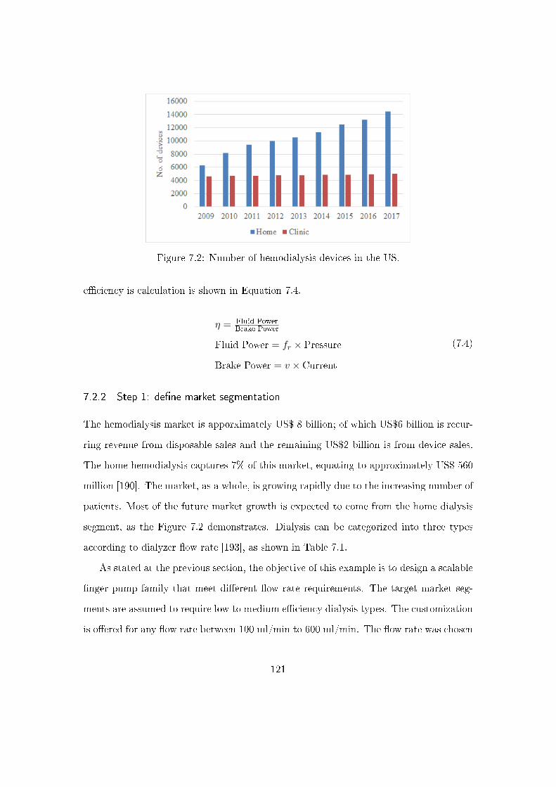
Figure 7.2: Number of hemodialysis devices in the US.
e�ciency is calculation is shown in Equation 7.4.
η = Fluid PowerBrake Power
Fluid Power = fr × Pressure
Brake Power = v × Current
(7.4)
7.2.2 Step 1: de�ne market segmentation
The hemodialysis market is apporximately US$ 8 billion; of which US$6 billion is recur-
ring revenue from disposable sales and the remaining US$2 billion is from device sales.
The home hemodialysis captures 7% of this market, equating to approximately US$ 560
million [190]. The market, as a whole, is growing rapidly due to the increasing number of
patients. Most of the future market growth is expected to come from the home dialysis
segment, as the Figure 7.2 demonstrates. Dialysis can be categorized into three types
according to dialyzer �ow rate [193], as shown in Table 7.1.
As stated at the previous section, the objective of this example is to design a scalable
�nger pump family that meet di�erent �ow rate requirements. The target market seg-
ments are assumed to require low to medium e�ciency dialysis types. The customization
is o�ered for any �ow rate between 100 ml/min to 600 ml/min. The �ow rate was chosen
121
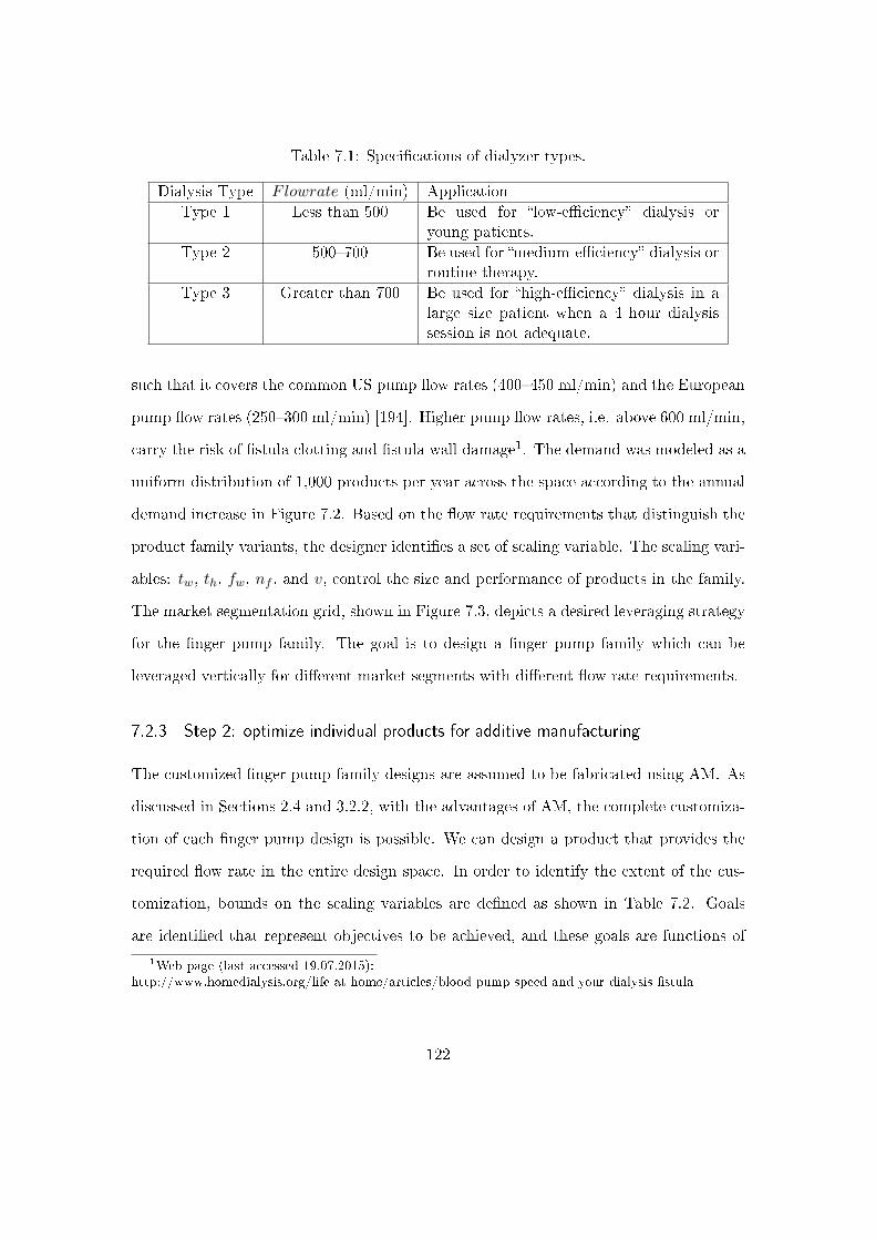
Table 7.1: Speci�cations of dialyzer types.
Dialysis Type Flowrate (ml/min) Application
Type 1 Less than 500 Be used for �low-e�ciency� dialysis oryoung patients.
Type 2 500�700 Be used for �medium-e�ciency� dialysis orroutine therapy.
Type 3 Greater than 700 Be used for �high-e�ciency� dialysis in alarge size patient when a 4 hour dialysissession is not adequate.
such that it covers the common US pump �ow rates (400�450 ml/min) and the European
pump �ow rates (250�300 ml/min) [194]. Higher pump �ow rates, i.e. above 600 ml/min,
carry the risk of �stula clotting and �stula wall damage1. The demand was modeled as a
uniform distribution of 1,000 products per year across the space according to the annual
demand increase in Figure 7.2. Based on the �ow rate requirements that distinguish the
product family variants, the designer identi�es a set of scaling variable. The scaling vari-
ables: tw, th, fw, nf , and v, control the size and performance of products in the family.
The market segmentation grid, shown in Figure 7.3, depicts a desired leveraging strategy
for the �nger pump family. The goal is to design a �nger pump family which can be
leveraged vertically for di�erent market segments with di�erent �ow rate requirements.
7.2.3 Step 2: optimize individual products for additive manufacturing
The customized �nger pump family designs are assumed to be fabricated using AM. As
discussed in Sections 2.4 and 3.2.2, with the advantages of AM, the complete customiza-
tion of each �nger pump design is possible. We can design a product that provides the
required �ow rate in the entire design space. In order to identify the extent of the cus-
tomization, bounds on the scaling variables are de�ned as shown in Table 7.2. Goals
are identi�ed that represent objectives to be achieved, and these goals are functions of
1Web page (last accessed 19.07.2015):http://www.homedialysis.org/life-at-home/articles/blood-pump-speed-and-your-dialysis-�stula
122
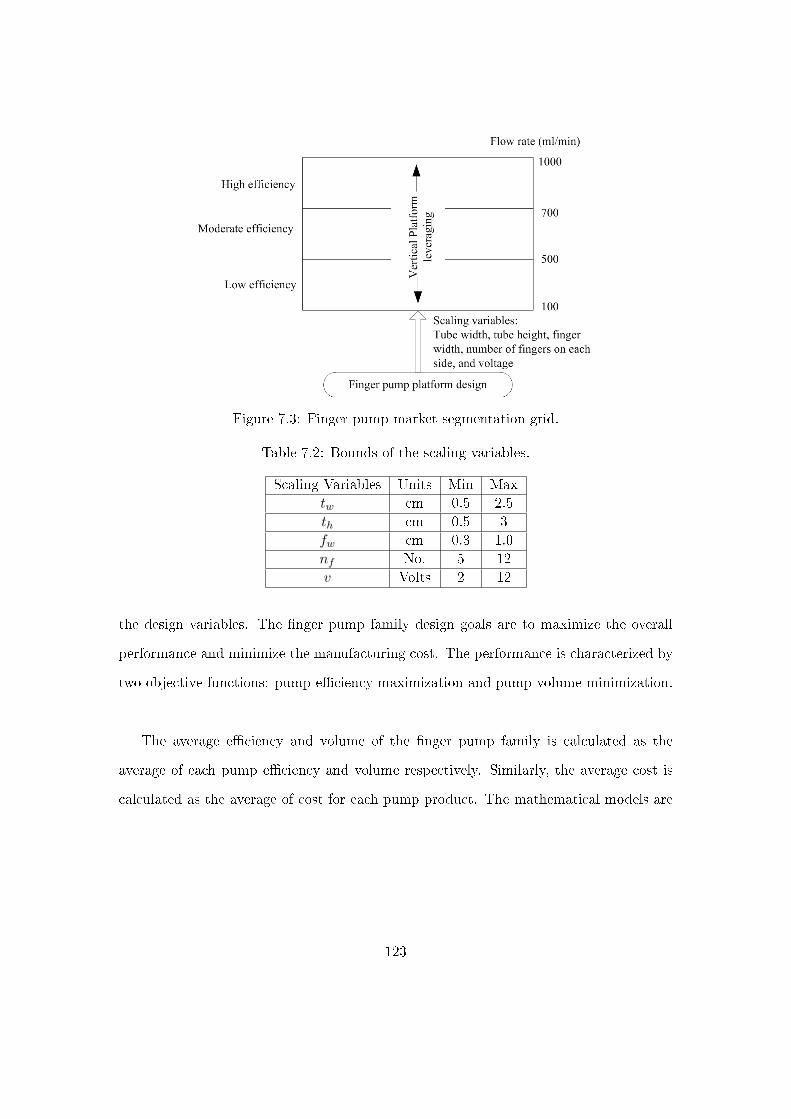
Figure 7.3: Finger pump market segmentation grid.
Table 7.2: Bounds of the scaling variables.
Scaling Variables Units Min Max
tw cm 0.5 2.5
th cm 0.5 3
fw cm 0.3 1.0
nf No. 5 12
v Volts 2 12
the design variables. The �nger pump family design goals are to maximize the overall
performance and minimize the manufacturing cost. The performance is characterized by
two objective functions: pump e�ciency maximization and pump volume minimization.
The average e�ciency and volume of the �nger pump family is calculated as the
average of each pump e�ciency and volume respectively. Similarly, the average cost is
calculated as the average of cost for each pump product. The mathematical models are
123
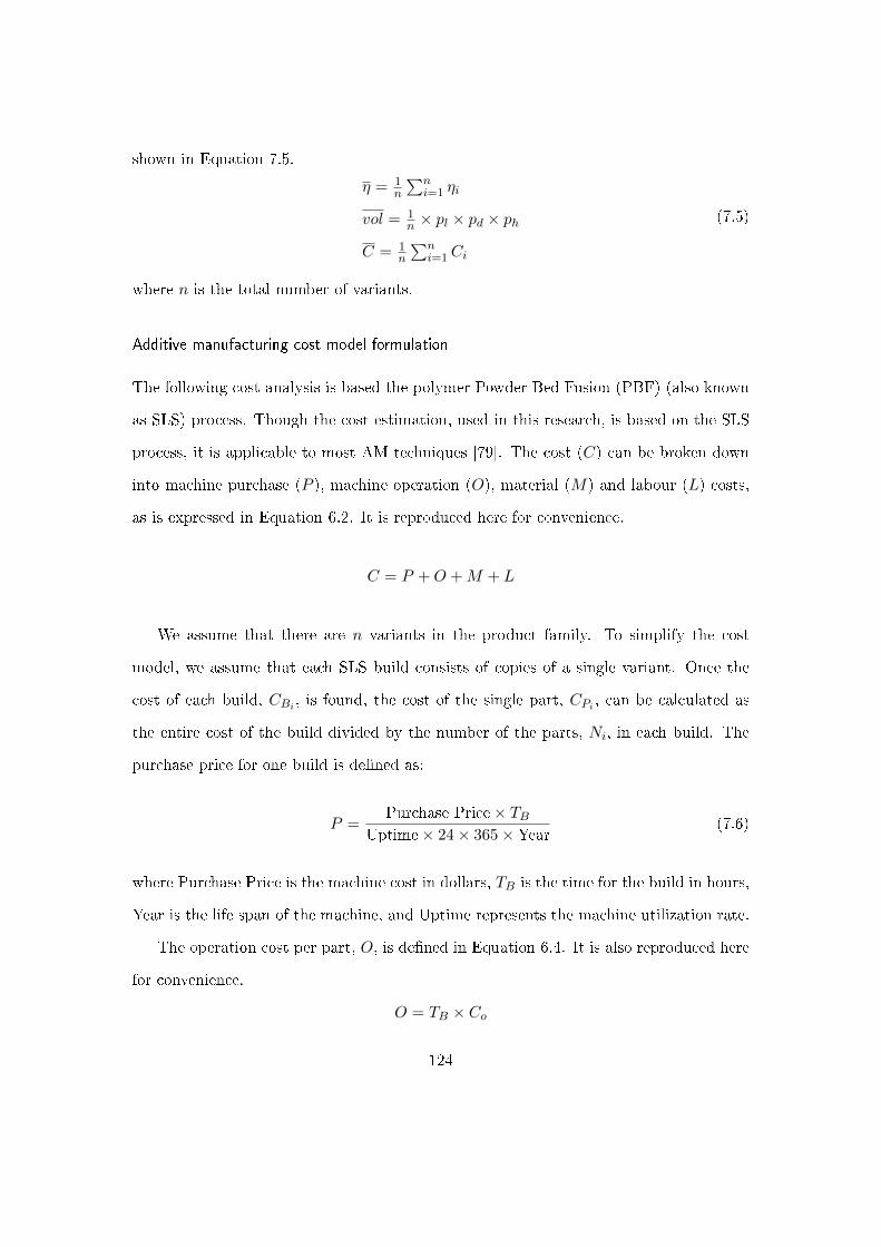
shown in Equation 7.5.
η = 1n
∑ni=1 ηi
vol = 1n × pl × pd × ph
C = 1n
∑ni=1Ci
(7.5)
where n is the total number of variants.
Additive manufacturing cost model formulation
The following cost analysis is based the polymer Powder Bed Fusion (PBF) (also known
as SLS) process. Though the cost estimation, used in this research, is based on the SLS
process, it is applicable to most AM techniques [79]. The cost (C) can be broken down
into machine purchase (P ), machine operation (O), material (M) and labour (L) costs,
as is expressed in Equation 6.2. It is reproduced here for convenience.
C = P +O +M + L
We assume that there are n variants in the product family. To simplify the cost
model, we assume that each SLS build consists of copies of a single variant. Once the
cost of each build, CBi , is found, the cost of the single part, CPi , can be calculated as
the entire cost of the build divided by the number of the parts, Ni, in each build. The
purchase price for one build is de�ned as:
P =Purchase Price× TB
Uptime× 24× 365×Year(7.6)
where Purchase Price is the machine cost in dollars, TB is the time for the build in hours,
Year is the life span of the machine, and Uptime represents the machine utilization rate.
The operation cost per part, O, is de�ned in Equation 6.4. It is also reproduced here
for convenience.
O = TB × Co
124

The operation cost is the cost that relates to machine maintenance, utility costs, factory
�oor space cost, and company overhead. Co is the operation cost rate.
The material cost (M) is given by:
M = (VB +WB)× ρ× Cm
WB = (1− σ)× (Vbed − VB)(7.7)
where VB is the volume of the entire build, sum of the N parts with volume (VP ) include
in the build; WB is the material volume wasted per build; ρ is the material mass density;
Cm is the material cost per kg; Vbed is the volume of the build platform that is express
by PLx, PLy, and PLz; PLx, PLy, and PLz are the size of the platform in x, y, and z
dimensions; σ ∈ [0, 1] is the recycle factor, depending on manufacturing process. In this
case, we assume σ = 0.8.
Labor cost is related to the time Tl required for technicians to set up the build, remove
fabricated parts, clean the parts, and get the machine ready for the next build.
L =TechSalary× TlAnnualworkh
(7.8)
where TechSalary is the technician salary per year and Annualworkh represents the an-
nual work hours.
Build time model
The time required to fabricate the parts is an important factor which in�uences the
operation cost. The manufacturing time per build can be expressed as the sum of scan
or deposition time (Txy), recoat time (Tz), and delay time (Td). We adapted the time
functions from Ru�o et al. [195]. The total manufacturing time TB is calculated as:
TB = Txy + Tz + Td (7.9)
125
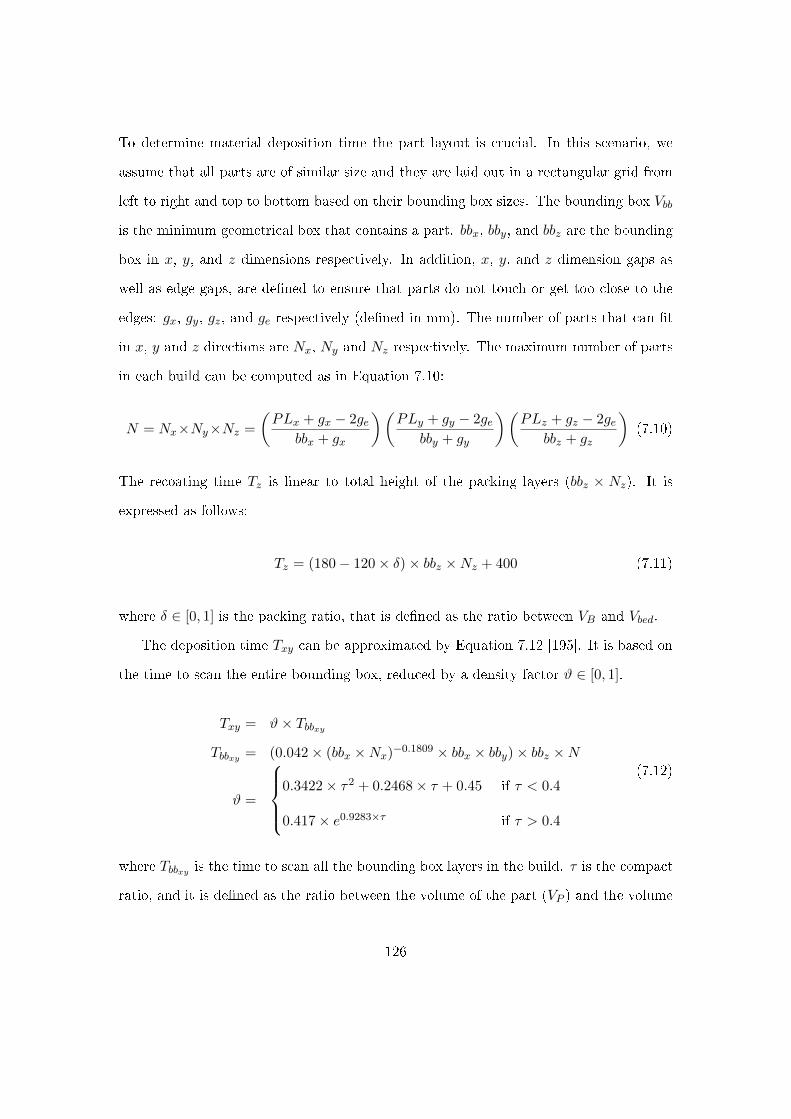
To determine material deposition time the part layout is crucial. In this scenario, we
assume that all parts are of similar size and they are laid out in a rectangular grid from
left to right and top to bottom based on their bounding box sizes. The bounding box Vbb
is the minimum geometrical box that contains a part. bbx, bby, and bbz are the bounding
box in x, y, and z dimensions respectively. In addition, x, y, and z dimension gaps as
well as edge gaps, are de�ned to ensure that parts do not touch or get too close to the
edges: gx, gy, gz, and ge respectively (de�ned in mm). The number of parts that can �t
in x, y and z directions are Nx, Ny and Nz respectively. The maximum number of parts
in each build can be computed as in Equation 7.10:
N = Nx×Ny×Nz =
(PLx + gx − 2ge
bbx + gx
)(PLy + gy − 2ge
bby + gy
)(PLz + gz − 2ge
bbz + gz
)(7.10)
The recoating time Tz is linear to total height of the packing layers (bbz × Nz). It is
expressed as follows:
Tz = (180− 120× δ)× bbz ×Nz + 400 (7.11)
where δ ∈ [0, 1] is the packing ratio, that is de�ned as the ratio between VB and Vbed.
The deposition time Txy can be approximated by Equation 7.12 [195]. It is based on
the time to scan the entire bounding box, reduced by a density factor ϑ ∈ [0, 1].
Txy = ϑ× Tbbxy
Tbbxy = (0.042× (bbx ×Nx)−0.1809 × bbx × bby)× bbz ×N
ϑ =
0.3422× τ2 + 0.2468× τ + 0.45 if τ < 0.4
0.417× e0.9283×τ if τ > 0.4
(7.12)
where Tbbxy is the time to scan all the bounding box layers in the build. τ is the compact
ratio, and it is de�ned as the ratio between the volume of the part (VP ) and the volume
126
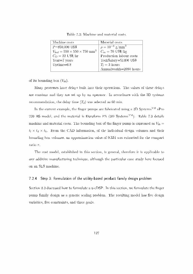
Table 7.3: Machine and material costs.
Machine costs Material costs
P=850,000 US$ ρ = 10−3 g/mm3
Vbed = 550× 550× 750 mm3 Cm = 70 US$/kgCO = 22 US$/hr Production labour costsYear=7 years TechSalary=51400 US$Uptime=0.8 Tl = 3 hours
Annualworkh=2080 hours
of its bounding box (Vbb).
Many processes have delays built into their operations. The values of these delays
are constant and they are set up by an operator. In accordance with the 3D systems
recommendation, the delay time (Td) was selected as 60 min.
In the current example, the �nger pumps are fabricated using a 3D SystemsTM sPro
230 HS model, and the material is Duraform PA (3D SystemsTM). Table 7.3 details
machine and material costs. The bounding box of the �nger pump is expressed as Vbb =
tl × td × th. From the CAD information, of the individual design volumes and their
bounding box volumes, an approximation value of 0.334 was extracted for the compact
ratio τ .
The cost model, established in this section, is general, therefore it is applicable to
any additive manufacturing technique, although the particular case study here focused
on an SLS machine.
7.2.4 Step 3: formulation of the utility-based product family design problem
Section 2.3 discussed how to formulate a u-cDSP. In this section, we formulate the �nger
pump family design as a generic scaling problem. The resulting model has �ve design
variables, �ve constraints, and three goals.
127
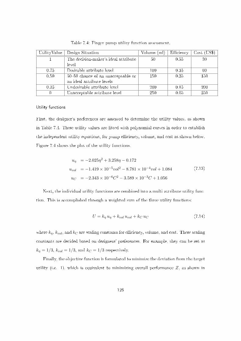
Table 7.4: Finger pump utility function assessment.
UtilityValue Design Situation Volume (ml) E�ciency Cost (US$)
1 The decision-maker's ideal attributelevel
50 0.55 30
0.75 Desirable attribute level 100 0.35 60
0.50 50�50 chance of an unacceptable oran ideal attribute levels
150 0.25 150
0.25 Undesirable attribute level 200 0.15 200
0 Unacceptable attribute level 250 0.05 250
Utility functions
First, the designer's preferences are assessed to determine the utility values, as shown
in Table 7.4. These utility values are �tted with polynomial curves in order to establish
the independent utility equations, for pump e�ciency, volume, and cost as shown below.
Figure 7.4 shows the plot of the utility functions.
uη = −2.025η2 + 3.258η − 0.172
uvol = −1.419× 10⁻⁵vol2 − 8.781× 10⁻⁴vol + 1.084
uC = −2.343× 10⁻⁶C2 − 3.589× 10⁻³C + 1.056
(7.13)
Next, the individual utility functions are combined into a multi-attribute utility func-
tion. This is accomplished through a weighted sum of the three utility functions:
U = kη uη + kvol uvol + kC uC (7.14)
where kη, kvol, and kC are scaling constants for e�ciency, volume, and cost. These scaling
constants are decided based on designers' preferences. For example, they can be set as
kη = 1/3, kvol = 1/3, and kC = 1/3 respectively.
Finally, the objective function is formulated to minimize the deviation from the target
utility (i.e. 1), which is equivalent to minimizing overall performance Z, as shown in
128
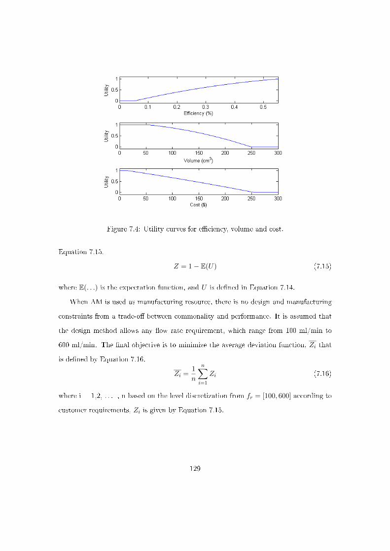
Figure 7.4: Utility curves for e�ciency, volume and cost.
Equation 7.15.
Z = 1− E(U) (7.15)
where E(. . .) is the expectation function, and U is de�ned in Equation 7.14.
When AM is used as manufacturing resource, there is no design and manufacturing
constraints from a trade-o� between commonality and performance. It is assumed that
the design method allows any �ow rate requirement, which range from 100 ml/min to
600 ml/min. The �nal objective is to minimize the average deviation function, Zi that
is de�ned by Equation 7.16.
Zi =1
n
n∑i=1
Zi (7.16)
where i = 1,2, . . . , n based on the level discretization from fr = [100, 600] according to
customer requirements, Zi is given by Equation 7.15.
129
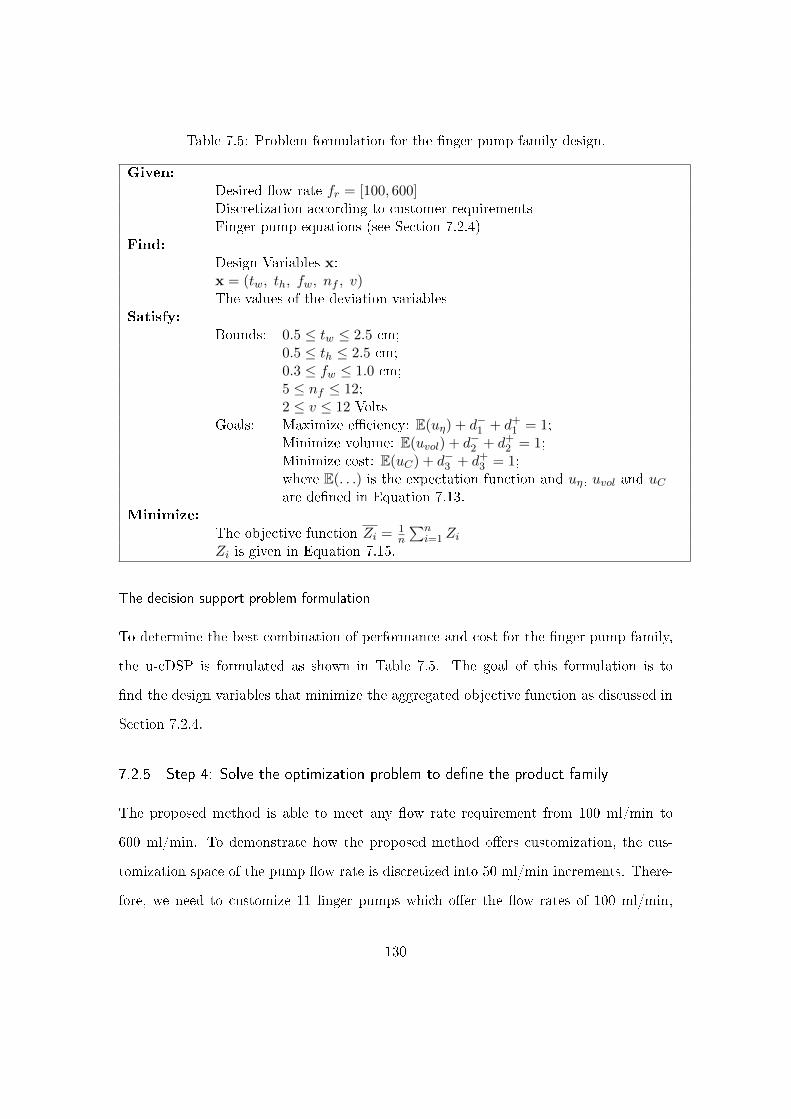
Table 7.5: Problem formulation for the �nger pump family design.
Given:
Desired �ow rate fr = [100, 600]Discretization according to customer requirementsFinger pump equations (see Section 7.2.4)
Find:
Design Variables x:x = (tw, th, fw, nf , v)The values of the deviation variables
Satisfy:
Bounds: 0.5 ≤ tw ≤ 2.5 cm;0.5 ≤ th ≤ 2.5 cm;0.3 ≤ fw ≤ 1.0 cm;5 ≤ nf ≤ 12;2 ≤ v ≤ 12 Volts
Goals: Maximize e�ciency: E(uη) + d−1 + d+1 = 1;
Minimize volume: E(uvol) + d−2 + d+2 = 1;
Minimize cost: E(uC) + d−3 + d+3 = 1;
where E(. . .) is the expectation function and uη, uvol and uCare de�ned in Equation 7.13.
Minimize:
The objective function Zi = 1n
∑ni=1 Zi
Zi is given in Equation 7.15.
The decision support problem formulation
To determine the best combination of performance and cost for the �nger pump family,
the u-cDSP is formulated as shown in Table 7.5. The goal of this formulation is to
�nd the design variables that minimize the aggregated objective function as discussed in
Section 7.2.4.
7.2.5 Step 4: Solve the optimization problem to de�ne the product family
The proposed method is able to meet any �ow rate requirement from 100 ml/min to
600 ml/min. To demonstrate how the proposed method o�ers customization, the cus-
tomization space of the pump �ow rate is discretized into 50 ml/min increments. There-
fore, we need to customize 11 �nger pumps which o�er the �ow rates of 100 ml/min,
130
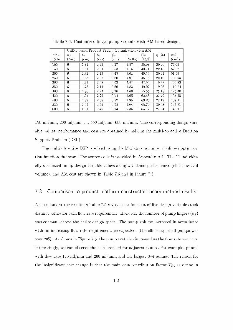
Table 7.6: Customized �nger pump variants with AM-based design.
Utility-based Product Family Optimization with AM
FlowRate
nf
(No.)tw(cm)
th(cm)
fw(cm)
v(Volts)
CP
(US$)η (%) vol
(cm3)
100 6 1.81 2.22 0.37 2.57 35.08 20.20 76.62
150 6 1.61 2.01 0.53 3.15 40.71 20.18 87.68
200 6 1.82 2.23 0.48 3.61 40.59 20.41 91.99
250 6 1.68 2.07 0.60 4.07 46.16 20.10 100.55
300 6 1.71 2.08 0.63 4.47 47.65 19.98 105.83
350 6 1.73 2.11 0.66 4.83 49.02 19.96 110.74
400 6 1.86 2.24 0.70 4.60 55.55 25.18 125.40
450 6 1.91 2.29 0.74 4.65 62.68 27.79 135.35
500 6 1.97 2.35 0.72 4.95 63.25 27.17 137.11
550 6 2.07 2.46 0.72 4.94 65.79 30.03 145.81
600 6 2.01 2.46 0.74 5.35 65.77 27.94 145.91
150 ml/min, 200 ml/min, ..., 550 ml/min, 600 ml/min. The corresponding design vari-
able values, performance and cost are obtained by solving the multi-objective Decision
Support Problem (DSP).
The multi-objective DSP is solved using the Matlab constrained nonlinear optimiza-
tion function, fmincon. The source code is provided in Appendix A.1. The 11 individu-
ally optimized pump design variable values along with their performance (e�ciency and
volume), and AM cost are shown in Table 7.6 and in Figure 7.5.
7.3 Comparison to product platform constructal theory method results
A close look at the results in Table 7.5 reveals that four out of �ve design variables took
distinct values for each �ow rate requirement. However, the number of pump �ngers (nf )
was constant across the entire design space. The pump volume increased in accordance
with an increasing �ow rate requirement, as expected. The e�ciency of all pumps was
over 20%. As shown in Figure 7.5, the pump cost also increased as the �ow rate went up.
Interestingly, we can observe the cost level o� for adjacent pumps, for example, pumps
with �ow rate 150 ml/min and 200 ml/min, and the largest 3�4 pumps. The reason for
the insigni�cant cost change is that the main cost contribution factor TB, as de�ne in
131
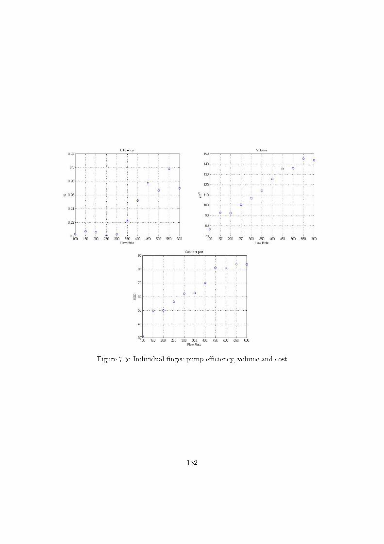
Figure 7.5: Individual �nger pump e�ciency, volume and cost
132
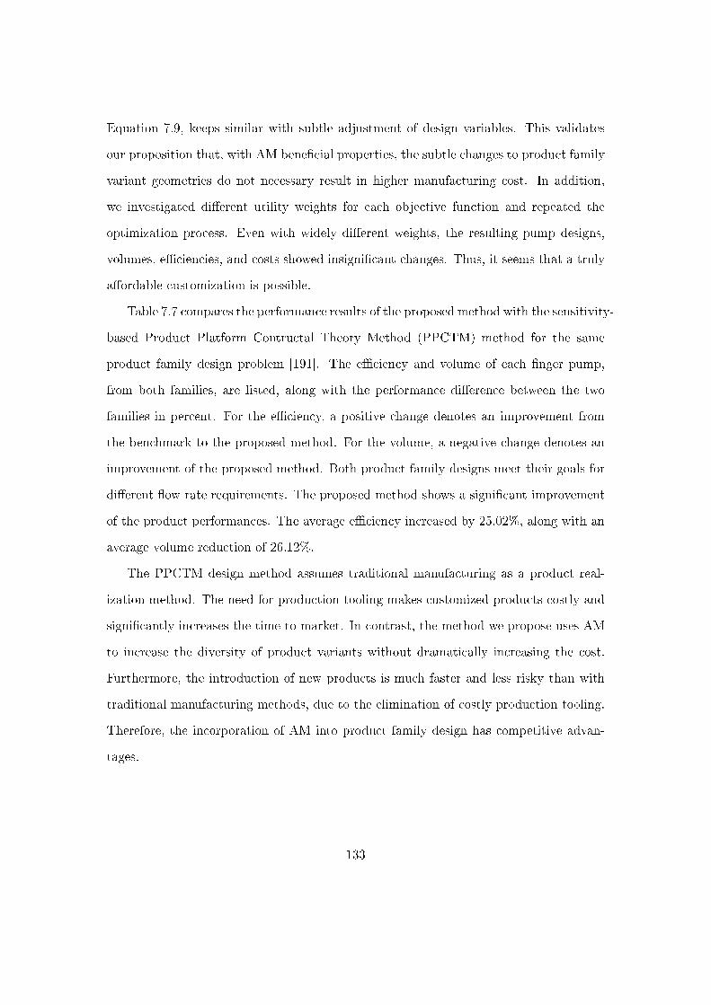
Equation 7.9, keeps similar with subtle adjustment of design variables. This validates
our proposition that, with AM bene�cial properties, the subtle changes to product family
variant geometries do not necessary result in higher manufacturing cost. In addition,
we investigated di�erent utility weights for each objective function and repeated the
optimization process. Even with widely di�erent weights, the resulting pump designs,
volumes, e�ciencies, and costs showed insigni�cant changes. Thus, it seems that a truly
a�ordable customization is possible.
Table 7.7 compares the performance results of the proposed method with the sensitivity-
based Product Platform Contructal Theory Method (PPCTM) method for the same
product family design problem [191]. The e�ciency and volume of each �nger pump,
from both families, are listed, along with the performance di�erence between the two
families in percent. For the e�ciency, a positive change denotes an improvement from
the benchmark to the proposed method. For the volume, a negative change denotes an
improvement of the proposed method. Both product family designs meet their goals for
di�erent �ow rate requirements. The proposed method shows a signi�cant improvement
of the product performances. The average e�ciency increased by 25.02%, along with an
average volume reduction of 26.12%.
The PPCTM design method assumes traditional manufacturing as a product real-
ization method. The need for production tooling makes customized products costly and
signi�cantly increases the time to market. In contrast, the method we propose uses AM
to increase the diversity of product variants without dramatically increasing the cost.
Furthermore, the introduction of new products is much faster and less risky than with
traditional manufacturing methods, due to the elimination of costly production tooling.
Therefore, the incorporation of AM into product family design has competitive advan-
tages.
133
Table 7.7: Customized �nger pump variants with AM-based design and comparison ofbaseline results.
Utility-based Product Fam-ily Optimization with AM
Sensitivity-basedPPCTM Pumps
Performance Im-provement (%)
FlowRate
CP
(US$)η (%) vol
(cm3)η (%) vol
(cm3)η (%) vol
(cm3)
100 35.08 20.20 76.62 19.1 125.9 4.50 -37.47
150 40.71 20.18 87.68 18.0 125.9 12.67 -32.93
200 40.59 20.41 91.99 19.8 142.5 12.98 -31.92
250 46.16 20.10 100.55 18.1 142.5 11.99 -30.19
300 47.65 19.98 105.83 19.8 154.8 0.81 -33.13
350 49.02 19.96 110.74 19.0 154.8 14.95 -27.67
400 55.55 25.18 125.40 20.0 163.1 7.80 -29.49
450 62.68 27.79 135.35 18.3 163.1 34.64 -23.34
500 63.25 27.17 137.11 19.9 173.4 17.89 -27.08
550 65.79 30.03 145.81 18.6 173.4 27.47 -24.64
600 65.77 27.94 145.91 17.3 173.4 18.27 -26.62
Average improvement: 25.02 -26.12
7.4 Summary
In this chapter, the proposed method is applied in full to the design of a �nger pump
family. The �nger pump family is based on a common scalable product platform that
is scaled around �ve design variables to provide di�erent �ow rates. The market seg-
mentation grid helps us to identify the targeting market segments and the appropriate
leveraging strategy. By introducing AM to the product family design, all constraints,
which arise in traditional product family designs from �nding a compromise between
commonality and performance of products, are eliminated. After determining both the
design space and objectives, the �nger pump family optimization problems are formu-
lated. The optimization step yields individual optimized products.
The proposed method achieved signi�cant performance improvement when compared
to the design methods that are constrained by traditional manufacturing processes and
therefore have to exploit the commonality between products. With the advantages of AM,
the customized �nger pumps can be fabricated in a more economic way when compare to
traditional manufacturing methods. Our method provides truly a�ordable individualized
134

designs without compromising the performance.
In conclusion, the proposed method provides a solution for improved mass customiza-
tion. It o�ers a�ordable customized designs without dramatically increasing the manu-
facturing cost. The integration of AM into product family design holds the promise of
reducing the current design for manufacturing e�orts. However, further research work is
necessary, because the use of AM for the production of functional products and assem-
blies is largely unexplored. We believe that a widespread adoption of AM would reduce
the machine and material costs due to the economies of scale. This would signi�cantly
reduce part costs and make AM an even more viable production route.
The next and �nal chapter presents a summary of achievements and contributions of
the work. A critical review of the current research and a discussion of possible directions
of future work are also provided.
135

Chapter 8
Closure: achievements and
recommendations
This thesis presents a data-driven product family design for Additive Manufacturing
(AM) method. The preceding text shows a theoretical introduction to the topic of AM
based product family design and practical case studies on implementation and testing.
In this chapter, the development and presentation of this method is brought to a close.
Section 8.1 summarizes the research work that has been done since August 2011. Section
8.2 explains and highlights the resulting contributions. Section 8.3 discusses limitations
and general shortcomings of the proposed methods. Possible directions of future work
are described in Section 8.4. Finally, Section 8.5 gives concluding remarks to close this
chapter and the thesis.
8.1 Research summary
To create a product is a mentally demanding process; to master it requires an enormous
amount of learning and focused dedication. This thesis outlines our knowledge and novel
ideas on the topic of data-driven product family design for AM. The research has focused
136
on data-driven product family design for AM method to improve mass customization.
As discussed in Chapter 1, the three primary research questions are:
Research question 1: How to enable more agile and more accurate decision-
making for market segmentation and product positioning?
Research question 2: How to incorporate AM into product family design
processes in order to facilitate customization in targeted market segments?
Research question 3: How to mathematically model and support product
platform decisions that involve multiple objectives?
To answer the �rst research question we conducted a critical literature review, which
is outlined in Section 2.2. During the literature review, we found that objective decision
making is of paramount importance in the current and in the future socio-economic
environment. Subjective and biased decision making leads to inferior results. In a product
design environment, such decisions may lead to sub-standard products which are less
competitive. As a consequence, we formulated the following research thesis: Data Mining
(DM) and machine learning technologies should be used to improve the objectiveness of
decision making processes. Chapters 4 and 5 presented both the theoretical and empirical
validation for the proposed Decision Support System (DSS). Section 4.2 established the
DSS to support the decision making in market segmentation and product positioning. To
augment this DSS, Section 5.2 proposed a framework to how to develop more rigorous
DSS for the decision support problems at hand. The automotive example was used
to test and validate the proposed method. While only demonstrated for one example,
it is asserted that the proposed DSS is generally applicable to other examples where
appropriate data is available.
For the second research question, the stand-of-the-art AM technologies were reviewed
and the impact on customization design was analyzed in Section 2.4. We found that the
AM based product family designs can operate in a much broader design space that
137
is free from constraints which arise in traditional product family designs from �nding
a compromise between commonality and performance of products. In order to take
advantage of the new manufacturing technology, the AM process model is established in
Section 6.2. In Section 6.3, the cantilever beam family design example demonstrates how
to the proposed model facilitate AM technologies to provide the customization.
To answer the third research question, we reviewed and compared Decision Support
Problem (DSP) methods. Both review process and review results are outlined in Section
2.3. For the scalable product family design, the individual targets for derivative products
can be aggregated into a weighted single target using the Utility-Based Compromise
Decision Support Problem (u-cDSP) method. The holistic method, which integrates
the three constructs, namely data-driven DSS for market segmentation and product
positioning, the AM process model for product family design, and u-cDSP method, is
presented in Chapter 2.3. The full implementation of the method is demonstrated in
Chapter 7 for the �nger pump family design. The benchmarking shows that the proposed
method achieved signi�cant performance improvement when compared to the design
methods that are constrained by tradition manufacturing processes and therefore need
to exploit commonality. It provides truly a�ordable customization without compromising
the product performances.
A summary of the research contributions is presented in the next section.
8.2 Research contributions
This research work is focused on the data-driven product family design for AM. The
primary contribution of this research is that it establishes a systematic framework that
seamlessly integrates AM into product family design to facilitate a�ordable customiza-
tion. The main result of the framework is the data-driven DSS to support market seg-
mentation and product positioning decision making. It is expected that the proposed
138
method will rede�ne how we think about customization in product family design. Other
major contributions include:
� Develop the data-driven DSS, called Decision Support System Database Explorer
(DSSDB Explorer), for automated market segmentation and product positioning
[138].
� Provide an unparalleled benchmark for 81 di�erent combinations of DM and ma-
chine learning techniques in the product family design domain [17].
� Provide a framework for the construction of a robust DSS.
� Rede�ne customization in product family design by incorporating AM technologies
[196].
� Develop a cost model for a family of products which are fabricated using Selective
Laser Sintering (SLS).
� Solve the multi-objective u-cDSP for product family design.
The contributions, associated with data-driven methods for market segmentation
and product positioning, lead to more robust design methods. DM and machine learning
methods have been widely used to solve product family design related problems. However,
most of these methods arbitrarily chose one or several techniques. The comparison of
the performance accuracy for di�erent DSSs in the product family design had never been
performed in such depth and breadth.
By incorporating AM for customization in product family design, we contributed
signi�cantly to both understanding and improving of mass customization. The improve-
ments come from the fact that the proposed method eliminates the constraints which
arise in traditional product family designs from �nding a compromise between common-
ality and individual performances. Our literature review shows that the proposed method
139
reduces a research gap, because there is a lack of structured approaches which utilize the
advantages of AM in product family design. Most of the existing product family design
methods focused on the trade-o�s between commonality and performance in the conven-
tional manufacturing context. However, the AM technologies rede�ne the way we think
about customization. The case study showed that the proposed AM based process model
for product family design translate the bene�ts of AM into improved customization and
cost reduction.
The formulation and solving of the u-cDSP are not of signi�cant value since these
techniques were adopted from the literature. However, extending them such that they
can be used to solve AM cost related problem is unique. Extending the u-cDSP technique
provides insights that can be used to improve existing methods.
In summary, the resulting data-driven product family design for AM method provides
additional knowledge of and a new concept for product family design and mass customiza-
tion. However, the proposed method is by no means without limitations. Towards this
end, a critical evaluation of the research is o�ered in the next section.
8.3 Limitations
In this section, the research itself is critically evaluated. The research is based on as-
sumptions, which might turn out to be false, and raise new, hopefully more re�ned,
questions.
For the application of the proposed method, there are two basic requirements. First,
the design variables or the input of the DSS are assumed to be known as priori. The
selection of these inputs limit the objective decision making. For example, in the auto-
motive case study in Chapters 4 and 5, it takes a decision making process to determine
which input to use and how to rank this input, such as Length, Width and Height.
The immediate question is: What design information are relevant and dominate for the
140
design process? The answer to this question is always centered on an implicit decision.
DM and machine learning technologies mechanize both clustering (market segmentation)
and classi�cation (product positioning) processes. These processes are mathematically
correct, i.e. they follow understandable algorithms. However, one limitation of these
algorithms is that they were invented by humans to solve speci�c problems, therefore
all of these algorithms have an inherent bias which diminishes their objectivity. Clas-
si�cation requires a training phase which is based on known data. In most cases this
training data was classi�ed through subjective decision making processes. Hence, during
the classi�cation phase the algorithm applies subjective decision making criteria in an
objective way. In terms of objectivity this is a major drawback. However the training
data comes from successful product designs, this, at least to some extent, validates the
training process. More abstractly speaking, the objective algorithm has learned good
decision making and this is now available access to wide range of designs.
In addition to the type of clustering and the distance measurement technique, results
of a clustering problem depend upon the selection of variables. The selection of �good�
variables may come about with a fair bit of trial and error complemented with the
analyst's intuition and background knowledge of the data set. Selection of �unwanted�
variables leads to clusters that do not present an informative structure. Additionally,
�goodness� of the clustering solution should be measured using various indices. This is
an inexact science and requires some degree of subjectivity.
Another limitation of the proposed method comes from the assumptions made when
we incorporated AM into the product family design process. Both guidelines and cri-
teria for the selection of either AM or traditional manufacturing technologies for part
realization are needed in the research community. For example, in Chapter 7, the fam-
ily of �nger pump assembles are assumed to automatically produced using SLS. The
cost analysis is based on the SLS process. The exploration of most cost e�ective way is
not conducted. For instance, which modules or components should be fabricated using
141

traditional manufacturing methods, and which ones should be fabricated using AM tech-
nologies. Furthermore, the demand is assumed to be uniform, the uncertainty in demand
does not taken into account.
Exploring the limitation of the use of the utility theory, it is noted that its use
might not be entirely warranted. The major weakness comes from its dependence on the
rationality and capability of the decision maker to e�ectively quantify their preferences
consistently.
Though the research has certain limitations, these limitations provide an avenue for
the future improvements. Recommendations for the future work in the areas of data-
driven product family design and AM for customization are discussed in the next section.
8.4 Recommendations and future work
The ability to meet diverse Customer Needs (CNs) and manufacture customized prod-
ucts or features with the e�ciency and a�ordable cost, is increasingly recognized as a
source of competitiveness in future markets. In order to achieve this capability, the de-
sign methodologies should concurrently consider product design, production design and
organization design. The key areas to be addressed include the following:
� Identify customized features, modules or full products based on CNs data,
� Design for Additive Manufacturing (DFAM) rules and principles to suggest which
AM technologies and materials should be used to provide customization,
� Concurrent design of product and process architectures,
� Systematic DSS that integrate market analysis, product design and manufacturing,
and supply chain.
� Improve the performance of the DSS by integrating and benchmarking even more
advanced decision support tools and utilities.
142
In the future, we aim to improve the performance of the proposed DSS by integrating
and benchmarking even more advanced decision support tools and utilities. This helps
us to address the problems that are posed by theoretical and practical management tasks
better. Future work will focus on extending the ideas of the system to cover all elements
of the product life cycle in the early stage of product development, in order to improve
the decision processes in concurrent engineering.
There is one good reason why data-driven methods for product family design will get
more and more important in the future. The reason comes from the fact that there is a
steady increase in the amount of available data. For example, new technology will bring
new sensors with higher resolution which are deployed pervasively. The latest data from
various sources is piled on top of legacy data. Most of the time there will be little or no
structure in this data. To make sense of this data will be the challenge which decides the
future of an enterprise. Even at current levels, it is impossible for humans to deal with
all that data. DM is necessary for enterprises to bene�t from the data. However even
with DM, the extracted information might be, and many cases still is, too complex or too
much removed from an understandable format. Arti�cial Intelligence (AI) techniques can
provide a problem driven data interpretation, for example by providing speci�c decision
support. In future only a consequent application of this new technology will ensure that
enterprises stay pro�table in a globalized economy.
8.5 Concluding remarks
Nothing is static. Everything is evolving. The research community in product family
design is no exception. The proposed method in this thesis is not an end in itself. It
provides a stepping stone for the future research work in related �elds of product family
design. We hope that the proposed method provides a framework to integrate data-
driven methods and new manufacturing technologies into product family design areas.
143

New problems and new demands in the product design arena will merge, new technologies
will change the way we solve the problems. New paths can be explored and new methods
can be developed which continue to advance the state-of-the-art in product design and
customization.
144

Bibliography
[1] M. H. Meyer and J. M. Utterback. �The product family and the dynamics of core
capability�. In: Sloan Management Review 34 (1993), pp. 29�47.
[2] D. Ben-Arieh, T. Easton, and A. M. Choubey. �Solving the multiple platforms con-
�guration problem�. In: International Journal of Production Research 47.7 (2009),
pp. 1969�1988.
[3] J. P. MacDu�e, K. Sethuraman, and M. L. Fisher. �Product variety and manufac-
turing performance: evidence from the international automotive assembly plant
study�. In: Management Science 42.3 (Mar. 1996), pp. 350�369.
[4] M. H. Meyer and A. P. Lehnerd. The power of product platforms: building value
and cost leadership. Free Press, 1997.
[5] A. Messac, M. P. Martinez, and T. W. Simpson. �E�ective product family design
using physical programming�. In: Engineering Optimization 34.3 (2002), pp. 245�
261.
[6] F. Alizon, K. Khadke, H. J. Thevenot, J. K. Gershenson, T. J. Marion, S. B.
Shooter, and T. W. Simpson. �Frameworks for product family design and devel-
opment�. In: Concurrent Engineering 15.2 (2007), pp. 187�199.
[7] B. J. Pine and S. Davis. Mass customization: the new frontier in business compe-
tition. Harvard Business School Press, 1999.
145
[8] D. Robertson and K. Ulrich. �Planning for product platforms.� In: Sloan Manage-
ment Review 39.4 (1998), pp. 19�31.
[9] T. W. Simpson, T. Marion, O. de Weck, K. Holtta-Otto, M. Kokkolaras, and S.
B. Shooter. �Platform-based design and development: current trends and needs in
industry�. In: Philadelphia, Pennsylvania, USA: ASME, 2006, pp. 801�810.
[10] T. W. Simpson, Z. Siddique, and J. Jiao. Product platform and product family
design: methods and applications. Birkhäuser, 2006.
[11] C. da Cunha, B. Agard, and A. Kusiak. �Design for cost: module-based mass
customization�. In: Automation Science and Engineering, IEEE Transactions on
4.3 (2007), pp. 350�359.
[12] M. Mu�atto and M. Roveda. �Developing product platforms:: analysis of the de-
velopment process�. In: Technovation 20.11 (2000), pp. 617�630.
[13] T. W. Simpson, C. C. Seepersad, and F. Mistree. �Balancing commonality and
performance within the concurrent design of multiple products in a product fam-
ily�. In: Concurrent Engineering 9.3 (2001), pp. 177�190.
[14] Z. Liu, Y. S. Wong, and K. S. Lee. �Modularity analysis and commonality design: a
framework for the top-down platform and product family design�. In: International
Journal of Production Research 48.12 (2010), pp. 3657�3680.
[15] S. K Moon, T. W. Simpson, and S. R. T. Kumara. �A methodology for knowledge
discovery to support product family design�. In: Annals of Operations Research
174.1 (2010), pp. 201�218.
[16] P. E. Green and Y.Wind.Marketing research and modeling : progress and prospects
: a tribute to Paul E. Green. International series in quantitative marketing: 14.
Boston : Kluwer Academic Publishers, c2004., 2004.
146

[17] N. Lei and S. K. Moon. �Decision support systems design for data-driven manage-
ment�. In: ASME 2014 International Design Engineering Technical Conferences
and Computers and Information in Engineering Conference, Volume 2A: 40th De-
sign Automation Conference. Bu�alo, New York, USA, Aug. 2014, DETC2014�
34871.
[18] N. Lei and S. K. Moon. �Objective product family design analysis using self-
organization map�. In: Industrial Engineering and Engineering Management (IEEM),
2012 IEEE International Conference on. Hong Kong, China, Dec. 2012, pp. 46�50.
[19] T. W. Simpson. �Product platform design and customization: status and promise�.
In: Arti�cial Intelligence for Engineering Design, Analysis and Manufacturing 18
(1 2004), pp. 3�20.
[20] Z. Dai and M. Scott. �Product platform design through sensitivity analysis and
cluster analysis�. In: Journal of Intelligent Manufacturing 18 (1 2007), pp. 97�113.
[21] M. E. Porter. �Technology and competitive advantage�. In: Journal of Business
Strategy 5.3 (1985), pp. 60�78.
[22] ASTM Standard. Standard Terminology for Additive Manufacturing Technologies.
10.04.
[23] J. (Roger) Jiao, T. Simpson, and Z. Siddique. �Product family design and platform-
based product development: a state-of-the-art review�. English. In: Journal of
Intelligent Manufacturing 18 (1 2007), pp. 5�29.
[24] J. Gonzalez-Zugasti, K. Otto, and J. Baker. �Assessing value in platformed prod-
uct family design�. In: Research in Engineering Design 13 (1 2001), pp. 30�41.
[25] X. Du, J. Jiao, and M. M. Tseng. �Architecture of product family: fundamentals
and methodology�. In: Concurrent Engineering 9.4 (2001), pp. 309�325.
147
[26] K. T. Ulrich and S. D. Eppinger. Product design and development / Karl T. Ulrich,
Steven D. Eppinger. Boston : McGraw-Hill Higher Education., 2008.
[27] S. K. Fixson. �Modularity and commonality research: past developments and fu-
ture opportunities�. In: Concurrent Engineering 15.2 (2007), pp. 85�111.
[28] V. B. Kreng and T.-P. Lee. �QFD-based modular product design with linear inte-
ger programming�a case study�. In: Journal of Engineering Design 15.3 (2004),
pp. 261�284.
[29] K. Fujita and H. Yoshida. �Product variety optimization simultaneously designing
module combination and module attributes�. In: Concurrent Engineering 12.2
(2004), pp. 105�118.
[30] C.-C. Huang and A. Kusiak. �Modularity in design of products and systems�. In:
Systems, Man and Cybernetics, Part A: Systems and Humans, IEEE Transactions
on 28.1 (Jan. 1998), pp. 66�77.
[31] X. Ye and J. K. Gershenson. �Attribute-based clustering methodology for product
family design�. In: Journal of Engineering Design 19.6 (2008), pp. 571�586.
[32] J. K. Gershenson, G. J. Prasad, and Y. Zhang. �Product modularity: measures
and design methods�. In: Journal of Engineering Design 15.1 (2004), pp. 33�51.
[33] S. K. Moon, S. R. T. Kumara, and T. W. Simpson. �Data mining and fuzzy
clustering to support product family design�. In: Proceedings of IDETC/CIE'06.
ASME, 2006, pp. 317�325.
[34] T. J. van Beek, M. S. Erden, and T. Tomiyama. �Modular design of mechatronic
systems with function modeling�. In: Mechatronics 20.8 (2010). Special Issue on
Theories and Methodologies for Mechatronics Design, pp. 850�863.
148

[35] T.-L. Yu, A. Yassine, and D. Goldberg. �An information theoretic method for
developing modular architectures using genetic algorithms�. English. In: Research
in Engineering Design 18.2 (2007), pp. 91�109.
[36] O. Durán, L. Pérez, and A. Batocchio. �Optimization of modular structures using
particle swarm optimization�. In: Expert Systems with Applications 39.3 (2012),
pp. 3507�3515.
[37] A. Jose and M. Tollenaere. �Modular and platform methods for product family
design: literature analysis�. In: Journal of Intelligent Manufacturing 16.3 (2005),
pp. 371�390.
[38] J. A. Joines, C. T. Culbreth, and R. E. King. �Manufacturing cell design: an
integer programming model employing genetic algorithms�. In: IIE Transactions
28.1 (1996), pp. 69�85.
[39] R. U. Nayak, W. Chen, and T. W. Simpson. �A variation-based method for prod-
uct family design�. In: Engineering Optimization 34.1 (2002), pp. 65�81.
[40] M. Martin and K. Ishii. �Design for variety: developing standardized and modu-
larized product platform architectures�. In: Research in Engineering Design 13.4
(2002), pp. 213�235.
[41] H. J. Thevenot and T. W. Simpson. �A comprehensive metric for evaluating com-
ponent commonality in a product family�. In: Proceedings of IDETC/CIE'06.
ASME, 2006, pp. 823�832.
[42] D. A. Collier. �The measurement and operating bene�ts of component part com-
monality�. In: Decision Sciences 12.1 (1981), pp. 85�96.
[43] H. J. Thevenot and T. W. Simpson. �Commonality indices for product family
design: a detailed comparison�. In: Journal of Engineering Design 17.2 (2006),
pp. 99�119.
149
[44] H. Wang, X. Zhu, H. Wang, S. J. Hu, Z. Lin, and G. Chen. �Multi-objective
optimization of product variety and manufacturing complexity in mixed-model
assembly systems�. In: Journal of Manufacturing Systems 30.1 (2011), pp. 16�27.
[45] V. R. R. Anil Kaul. �Research for product positioning and design decisions: An in-
tegrative review�. In: International Journal of Research in Marketing 12.4 (1995),
pp. 293�320.
[46] N. F. Piercy and N. A. Morgan. �Strategic and operational market segmentation:
a managerial analysis�. In: Journal of Strategic Marketing 1.2 (1993), pp. 123�140.
[47] K. Sausen, T. Tomczak, and A. Herrmann. �Development of a taxonomy of strate-
gic market segmentation: a framework for bridging the implementation gap be-
tween normative segmentation and business practice�. In: Journal of Strategic
Marketing 13.3 (2005), pp. 151�173.
[48] C. J. Romanowski, R. Nagi, and M. Sudit. �Data mining in an engineering design
environment: OR applications from graph matching�. In: Computers & Operations
Research 33.11 (2006), pp. 3150�3160.
[49] D. Braha. Data mining for design and manufacturing : methods and applications
/ edited by Dan Braha. Massive computing: v. 3. Boston : Kluwer Academic Pub-
lishers, 2001.
[50] D. J. Kim, D. L. Ferrin, and H. R. Rao. �A trust-based consumer decision-making
model in electronic commerce: the role of trust, perceived risk, and their an-
tecedents�. In: Decision Support Systems 44.2 (2008), pp. 544�564.
[51] A. Kusiak. �Data mining: manufacturing and service applications�. In: Interna-
tional Journal of Production Research 44 (2006), pp. 4175�4191.
[52] C. S. Tucker, H. M. Kim, D. E. Barker, and Y. Zhang. �A ReliefF attribute
weighting and X-means clustering methodology for top-down product family op-
timization.� In: Engineering Optimization 42.7 (2010), pp. 593�616.
150
[53] P. McCorduck. Machines who think : a personal inquiry into the history and
prospects of arti�cial intelligence. Natick, Mass. : A.K. Peters., 2004.
[54] C. R. Westphal and T. Blaxton. Data mining solutions : methods and tools for
solving real-world problems / Christopher Westphal, Teresa Blaxton. New York :
Wiley, 1998.
[55] Y. Kim and W. Street. �An intelligent system for customer targeting: a data
mining approach�. In: Decision Support Systems 37.2 (2004), pp. 215�228.
[56] T. Raeder and N. V. Chawla. �Market basket analysis with networks�. In: Social
Network Analysis and Mining 1.2 (2010), pp. 97�113.
[57] B. Agard and A. Kusiak. �Data-mining-based methodology for the design of
product families�. In: International Journal of Production Research 42.15 (2004),
pp. 2955�2969.
[58] L. Yu and L. Wang. �Product portfolio identi�cation with data mining based
on multi-objective GA�. In: Journal of Intelligent Manufacturing 21.6 (2010),
pp. 797�810.
[59] C.-H. Chen, L. P. Khoo, and W. Yan. �An investigation into a�ective design using
sorting technique and Kohonen self-organising map�. In: Advances in Engineering
Software 37.5 (2006), pp. 334�349.
[60] R. J. Kuo, L. M. Ho, and C. M. Hu. �Integration of self-organizing feature map
and K-means algorithm for market segmentation�. In: Computers & Operations
Research 29.11 (2002), pp. 1475�1493.
[61] C. Y. Tsai and C. C. Chiu. �A purchase-based market segmentation methodology�.
In: Expert Systems with Applications 27.2 (2004), pp. 265�276.
151
[62] S. Han, Y. Ye, X. Fu, and Z. Chen. �Category role aided market segmentation
approach to convenience store chain category management�. In: Decision Support
Systems 57 (2014), pp. 296�308.
[63] W. B. V. Venugopal. �Neural networks and statistical techniques in marketing
research: a conceptual comparison�. In: Marketing Intelligence & Planning 12.7
(1994), pp. 30�38.
[64] K. Wang, S. Tong, B. Eynard, L. Roucoules, and N. Matta. �Review on application
of data mining in product design and manufacturing�. In: Fuzzy Systems and
Knowledge Discovery (FSKD). Fourth International Conference on. Vol. 4. 2007,
pp. 613�618.
[65] R. E. Plank. �A critical review of industrial market segmentation�. In: Industrial
Marketing Management 14.2 (1985), pp. 79�91.
[66] N. Lei and S. K. Moon. �A decision support system for market segment driven
product design�. In: Proceedings of the 19th International Conference on Engineer-
ing Design (ICED13), Design for Harmonies, Vol.9: Design Methods and Tools.
ICED. Seoul, Korea, Aug. 2013, pp. 177�186.
[67] J.-L. Seng and T. Chen. �An analytic approach to select data mining for business
decision�. In: Expert Systems with Applications 37.12 (2010), pp. 8042�8057.
[68] P. Balakrishnan, M. C. Cooper, V. S. Jacob, and P. A. Lewis. �Comparative per-
formance of the {FSCL} neural net and K-means algorithm for market segmenta-
tion�. In: European Journal of Operational Research 93.2 (1996). Neural Networks
and Operations Research/Management Science, pp. 346�357.
[69] H. Hruschka and M. Natter. �Comparing performance of feedforward neural nets
and K-means for cluster-based market segmentation�. In: European Journal of
Operational Research 114.2 (1999), pp. 346�353.
152
[70] R. J. Kuo, M. J. Wang, and T. W. Huang. �An application of particle swarm
optimization algorithm to clustering analysis�. In: Soft Computing 15.3 (2011),
pp. 533�542.
[71] G. A. Hazelrigg. Systems engineering : an approach to information-based design.
Prentice-Hall international series in industrial and systems engineering. Upper
Saddle River, NJ : Prentice Hall, c1996., 1996.
[72] F. Mistree, O. F Hughes, and B. A. Bras. �The compromise decision support prob-
lem and the adaptive linear programming algorithm�. In: Structural optimization:
status and promise. Ed. by M. P. Kamat. Washington, DC: The American Insti-
tute of Aeronautics and Astronautics, 1992, pp. 251�290.
[73] C. C. Seepersad. �The utility-based compromise decision support problem with
applications in product platform design�. Master thesis. Atlanta, GA, USA: GW
Woodru� School of Mechanical Engineering, Georgia Institute of Technology,
2001.
[74] R. L. Keeney and H. Rai�a. Decisions with multiple objectives : preferences and
value tradeo�s. Cambridge University Press, 1993.
[75] C. C. Seepersad, F. Mistree, and J. K. Allen. �A quantitative approach for design-
ing multiple product platforms for an evolving portfolio of products�. In: Proceed-
ings of ASME 2002 International Design Engineering Technical Conferences and
Computers and Information in Engineering Conference on. Montreal, Quebec,
Canada: ASME, 2002, pp. 579�592.
[76] M. G. Fernandez, C. C. Seepersad, D. W. Rosen, J. K. Allen, and F. Mistree.
�Utility-based decision, support for selection in engineering design�. In: Proceed-
ings of the 2001 ASME Design Engineering Technical Conferences. Pittsburgh,
PA, USA, 2001, DETC2001/DAC�21106.
153
[77] J. Jiao and M. Tseng. �A methodology of developing product family architecture
for mass customization�. English. In: Journal of Intelligent Manufacturing 10.1
(1999), pp. 3�20.
[78] C. B. Williams, J. K. Allen, D. W. Rosen, and F. Mistree. �Designing platforms
for customizable products and processes in markets of non-uniform demand�. In:
Concurrent Engineering 15.2 (2007), pp. 201�216.
[79] I. Gibson, D. W. Rosen, and B. Stucker. Additive manufacturing technologies:
rapid prototyping to direct digital manufacturing. Boston, MA : Springer Sci-
ence+Business Media, LLC 2010, 2010.
[80] N. Hopkinson, R. J. M. Hague, and P. M. Dickens. Rapid manufacturing : an
industrial revolution for the digital age. Ed. by N. Hopkinson, R. J. M. Hague,
and P. M. Dickens. Chichester, England : John Wiley, c2006., 2006.
[81] P. F. Jacobs. Rapid prototyping and manufacturing: fundamentals of stereolithog-
raphy. New York, NY, USA: McGraw-Hill, Inc., 1993.
[82] J. Holmström, J. Partanen, J. Tuomi, and M. Walter. �Rapid manufacturing in the
spare parts supply chain�. In: Journal of Manufacturing Technology Management
21.6 (2010), pp. 687�697.
[83] C. Thomas, T. Ga�ney, S. Kaza, and C. Lee. �Rapid prototyping of large scale
aerospace structures�. In: Aerospace Applications Conference, 1996. Proceedings.,
1996 IEEE. Vol. 4. Feb. 1996, pp. 219�230.
[84] S. K. Moon, Y. E. Tan, J. Hwang, and Y.-J. Yoon. �Application of 3D printing
technology for designing light-weight unmanned aerial vehicle wing structures�.
English. In: International Journal of Precision Engineering and Manufacturing-
Green Technology 1.3 (2014), pp. 223�228.
154
[85] Y. Ding, H. Lan, J. Hong, and D. Wu. �An integrated manufacturing system for
rapid tooling based on rapid prototyping�. In: Robotics and Computer-Integrated
Manufacturing 20.4 (2004), pp. 281�288.
[86] F. Rengier, A. Mehndiratta, H. von Tengg-Kobligk, C. M. Zechmann, R. Unterhin-
ninghofen, H.-U. Kauczor, and F. L. Giesel. �3D printing based on imaging data:
review of medical applications�. English. In: International Journal of Computer
Assisted Radiology and Surgery 5.4 (2010), pp. 335�341.
[87] D. W. Rosen. �Computer-aided design for additive manufacturing of cellular struc-
tures�. In: Computer-Aided Design and Applications 4.5 (2007), pp. 585�594.
[88] R. Hague, S. Mansour, and N. Saleh. �Material and design considerations for rapid
manufacturing�. In: International Journal of Production Research 42.22 (2004),
pp. 4691�4708.
[89] X. Su, Y. Yang, D. Xiao, and Y. Chen. �Processability investigatation of non-
assembly mechanisms for powder bed fusion process�. English. In: The Interna-
tional Journal of Advanced Manufacturing Technology 64.5-8 (2013), pp. 1193�
1200.
[90] S. Bin Maidin, I. Campbell, and E. Pei. �Development of a design feature database
to support design for additive manufacturing�. In: Assembly Automation 32.3
(2012), pp. 235�244.
[91] F. Xu, Y. S. Wong, and H. T. Loh. �Toward generic models for comparative
evaluation and process selection in rapid prototyping and manufacturing�. In:
Journal of Manufacturing Systems 19.5 (2001), pp. 283�296.
[92] N. Lei, S. K. Moon, and G. Bi. �Additive manufacturing and topology optimiza-
tion to support product family design�. English. In: High Value Manufacturing:
Advanced Research in Virtual and Rapid Prototyping: Proceedings of the 6th In-
155
ternational Conference on Advanced Research in Virtual and Rapid Prototyping,
Leiria, Portugal. Ed. by P. Bartolo et al. CRC Press, 2013, pp. 505�510.
[93] R. Rezaie, M. Badrossamay, A. Ghaie, and H. Moosavi. �Topology optimization
for fused deposition modeling process�. In: Procedia CIRP 6.0 (2013). Proceedings
of the Seventeenth CIRP Conference on Electro Physical and Chemical Machining
(ISEM), pp. 521�526.
[94] Siemens Hearing Instruments, Inc. www.siemens-hearing.com. Accessed: 2015-
04-30.
[95] J. Jiao and Y. Zhang. �Product portfolio identi�cation based on association rule
mining�. In: Computer-Aided Design 37.2 (2005), pp. 149�172.
[96] G. Hernandez, J. K. Allen, and F. Mistree. �Platform design for customizable
products as a problem of access in a geometric space�. In: Engineering Optimiza-
tion 35.3 (2003), pp. 229�254.
[97] C. B. Williams. �Platform design for customizable product and processes with
non-uniform demand�. Master thesis. Atlanta, GA, USA: GW Woodru� School of
Mechanical Engineering, Georgia Institute of Technology, 2003.
[98] V. Krishnan and K. T. Ulrich. �Product development decisions: a review of the
literature�. In: Management Science 47.1 (2001), pp. 1�21.
[99] R. Varadarajan. �Strategic marketing and marketing strategy: domain, de�ni-
tion, fundamental issues and foundational premises�. English. In: Journal of the
Academy of Marketing Science 38.2 (2010), pp. 119�140.
[100] R. Howard and B.-C. Björk. �Building information modelling � experts' views on
standardisation and industry deployment�. In: Advanced Engineering Informatics
22.2 (2008), pp. 271�280.
156
[101] L. Xu, Z. Li, S. Li, and F. Tang. �A decision support system for product design in
concurrent engineering�. In: Decision Support Systems 42.4 (2007), pp. 2029�2042.
[102] G. Marakas. Decision support systems in the 21st century. Prentice Hall, 2003.
[103] D. J. Power. A brief history of decision support system @ONLINE Last accessed
December 2013: http://DSSResources.com/history/dsshistory.html. 2007.
[104] L. Eeckhout and K. D. Bosschere. �How accurate should early design stage pow-
er/performance tools be? A case study with statistical simulation�. In: Journal of
Systems and Software 73.1 (2004), pp. 45�62.
[105] B. Prasad. �Review of QFD and related deployment techniques�. In: Journal of
manufacturing Systems 17.3 (1998), pp. 221�234.
[106] T. L. Saaty. Fundamentals of decision making and priority theory with the analytic
hierarchy process / Thomas L. Saaty. AHP series: vol. 6. Pittsburgh, PA : RWS
Publications., 2000.
[107] N. P. Suh. �A theory of innovation and case study�. In: International Journal of
Innovation Management 14.05 (2010), pp. 893�913.
[108] Y. Zare Mehrjerdi. �Six-sigma: methodology, tools and its future�. In: Assembly
Automation 31.1 (2011), pp. 79�88.
[109] R. Kazemzadeh, M. Behzadian, M. Aghdasi, and A. Albadvi. �Integration of mar-
keting research techniques into house of quality and product family design�. In:
The International Journal of Advanced Manufacturing Technology 41.9-10 (2009),
pp. 1019�1033.
[110] S. Aungst, R. Barton, and D. Wilson. �The virtual integrated design method�. In:
Quality Engineering 15.4 (2003), pp. 565�579.
157
[111] B. Besharati, S. Azarm, and P. Kannan. �A decision support system for product
design selection: a generalized purchase modeling approach�. In: Decision Support
Systems 42.1 (2006), pp. 333�350.
[112] J. Gosling. The Java language speci�cation. Java series. Upper Saddle River, NJ
: Addison-Wesley, c2005., 2005.
[113] S. Chaudhuri, U. Dayal, and V. Ganti. �Database technology for decision support
systems�. In: Computer 34.12 (2001), pp. 48�55.
[114] P. DuBois. MySQL [electronic resource] : the de�nitive guide to using, program-
ming, and administering MySQL4 / Paul DuBois. Developer's library. Boston,
MA : ProQuest Information and Learning Company, 2003., 2003.
[115] I. T. Jolli�e. Principal component analysis. Springer Series in Statistics. Springer,
2002.
[116] H. Zha, X. He, C. H. Q. Ding, M. Gu, and H. D. Simon. �Spectral relaxation for
K-means clustering.� In: Proceedings of Neural Information Processing Systems.
Vol. 14. Vancouver, Canada: NIPS, Dec. 2001, pp. 1057�1064.
[117] R. B. Cattell. �The scree test for the number of factors�. In: Multivariate Behav-
ioral Research 1.2 (1966), pp. 245�276.
[118] MATLAB version 8 (R2012b). http://www.mathworks.com/help/. Natick, Mas-
sachusetts: The MathWorks Inc., 2012.
[119] J. MacQueen. �Some methods for classi�cation and analysis of multivariate obser-
vations�. In: Proceedings of the �fth Berkeley symposium on mathematical statistics
and probability. Vol. 1. California, USA. 1967, p. 14.
[120] J. A. Hartigan and M. A. Wong. �Algorithm AS 136: a K-means clustering algo-
rithm�. In: Journal of the Royal Statistical Society. Series C (Applied Statistics)
28.1 (1979), pp. 100�108.
158
[121] C. Ding and X. He. �K-means clustering via principal component analysis�. In:
Proceedings of the twenty-�rst international conference on Machine learning. ICML
'04. New York, NY, USA: ACM, 2004.
[122] P. J. Rousseeuw. �Silhouettes: A graphical aid to the interpretation and validation
of cluster analysis�. In: Journal of Computational and Applied Mathematics 20.0
(1987), pp. 53�65.
[123] A. Struyf, M. Hubert, and P. J. Rousseeuw. �Integrating robust clustering tech-
niques in S-PLUS�. In: Computational Statistics & Data Analysis 26.1 (1997),
pp. 17�37.
[124] M. J. Kearns and U. V. Vazirani. An introduction to computational learning theory.
MIT Press, Aug. 1994.
[125] Y. Freund and R. Schapire. �A desicion-theoretic generalization of on-line learn-
ing and an application to boosting�. In: Computational Learning Theory. Ed. by
P. Vitányi. Vol. 904. Lecture Notes in Computer Science. Springer Berlin / Hei-
delberg, 1995, pp. 23�37.
[126] W. Iba and P. Langley. �Induction of one-level decision trees�. In: Proceedings of
the Ninth International Workshop on Machine Learning. ML '92. San Francisco,
CA, USA: Morgan Kaufmann Publishers Inc., 1992, pp. 233�240.
[127] U. R. Acharya, O. Faust, N. Adib Kadri, J. S. Suri, and W. Yu. �Automated
identi�cation of normal and diabetes heart rate signals using nonlinear measures�.
In: Computers in Biology and Medicine 43.10 (2013), pp. 1523�1529.
[128] J. Friedman, T. Hastie, and R. Tibshirani. �Additive logistic regression: a statis-
tical view of boosting�. In: The Annals of Statistics 28.2 (2000), pp. 337�407.
[129] L. Breiman. �Bagging predictors�. In:Machine Learning 24.2 (Aug. 1996), pp. 123�
140.
159
[130] S. Paris. Multiclass GentleAdaboosting. Matlab central, �le exchange. 2012.
[131] S. Geisser. Predictive inference. Monographs on Statistics and Applied Probabil-
ity. Taylor & Francis, 1993.
[132] C. Scha�er. �Selecting a classi�cation method by cross-validation�. In: Machine
Learning 13.1 (1993), pp. 135�143.
[133] R. Kohavi. �A study of cross-validation and bootstrap for accuracy estimation
and model selection�. In: Proceedings of the 14th international joint conference on
Arti�cial intelligence - Volume 2. IJCAI'95. Montreal, Quebec, Canada: Morgan
Kaufmann Publishers Inc. San Francisco, CA, USA, 1995, pp. 1137�1143.
[134] L. Breiman. Classi�cation and regression trees. Wadsworth statistics/probability
series. Wadsworth International Group, 1984.
[135] National Highway Tra�c Safety Administration. 5-Star Ratings FAQ @ONLINE
Last accessed June 2014: www.safercar.gov/Vehicle+Shoppers/5-Star+FAQ.
[136] Ward's Automotive Group, a division of Penton Media Inc. 10 Model Car U.S.
Speci�cations and Prices � Final. Ward_LV_Specs_2010.xls. 2010.
[137] S. jin Wang, A. Mathew, Y. Chen, L. feng Xi, L. Ma, and J. Lee. �Empirical
analysis of support vector machine ensemble classi�ers�. In: Expert Systems with
Applications 36.3, Part 2 (2009), pp. 6466�6476.
[138] N. Lei and S. K. Moon. �A decision support system for market-driven product
positioning and design�. In: Decision Support Systems 69.0 (2015), pp. 82�91.
[139] D. J. Power and R. Sharda. �Model-driven decision support systems: concepts and
research directions�. In: Decision Support Systems 43.3 (2007), pp. 1044�1061.
[140] A. T. Olewnik and K. E. Lewis. �On validating design decision methodologies�.
In: ASME DETC, Computers and Information in Engineering Conference. 2003.
160
[141] G. F. Smith. �Beyond critical thinking and decision making: teaching business
students how to think�. In: Journal of Management Education 27.1 (2003), pp. 24�
51.
[142] T. W. Simpson, J. Peplinski, P. N. Koch, and J. K. Allen. �On the use of statistics
in design and the implications for deterministic computer experiments�. In: Design
Theory and Methodology-DTM'97. 1997, pp. 14�17.
[143] M. G. Fernández, C. C. Seepersad, D. W. Rosen, J. K. Allen, and F. Mistree.
�Decision support in concurrent engineering � the utility-based selection decision
support problem�. In: Concurrent Engineering 13.1 (2005), pp. 13�27.
[144] K. N. Otto and E. K. Antonsson. �The method of imprecision compared to util-
ity theory for design selection problems�. In: Design Theory and Methodology�
DTM'93. 1993, pp. 167�173.
[145] E. Brynjolfsson, L. M. Hitt, and H. H. Kim. �Strength in numbers: how does
data-driven decision making a�ect �rm performance?� In: Proceedings of the in-
ternational conference on information systems. 13. Shanghai, China, Dec. 2011.
[146] D. J. Power. �Understanding data-driven decision support systems�. In: Informa-
tion Systems Management 25.2 (2008), pp. 149�154.
[147] L. J. Skitka, K. L. Mosier, and M. Burdick. �Does automation bias decision-
making?� In: International Journal of Human-Computer Studies 51.5 (1999), pp. 991�
1006.
[148] F. Camastra. �Data dimensionality estimation methods: a survey�. In: Pattern
Recognition 36.12 (2003), pp. 2945�2954.
[149] W. A. Broock, J. A. Scheinkman, W. D. Dechert, and B. LeBaron. �A test for
independence based on the correlation dimension�. In: Econometric Reviews 15.3
(1996), pp. 197�235.
161

[150] K. Fukunaga and D. R. Olsen. �An algorithm for �nding intrinsic dimensionality
of data�. In: Computers, IEEE Transactions on C-20.2 (1971), pp. 176�183.
[151] E. Levina and P. J. Bickel. �Maximum likelihood estimation of intrinsic dimen-
sion�. In: Advances in neural information processing systems. 2004, pp. 777�784.
[152] J. A. Costa and A. O. Hero. �Geodesic entropic graphs for dimension and entropy
estimation in manifold learning�. In: Signal Processing, IEEE Transactions on
52.8 (2004), pp. 2210�2221.
[153] L. J. P. Van der Maaten, E. O. Postma, and H. J. Van den Herik. �Dimensionality
reduction: a comparative review�. In: Technical Report TiCC TR 2009-005 (2009).
[154] H. Hotelling. �Analysis of a complex of statistical variables into principal compo-
nents.� In: Journal of educational psychology 24.6 (1933), p. 417.
[155] J. B. Kruskal. �Multidimensional scaling by optimizing goodness of �t to a non-
metric hypothesis�. In: Psychometrika 29.1 (1964), pp. 1�27.
[156] J. W. Sammon. �A nonlinear mapping for data structure analysis�. In: Computers,
IEEE Transactions on C-18.5 (1969), pp. 401�409.
[157] S. T. Roweis and L. K. Saul. �Nonlinear dimensionality reduction by locally linear
embedding�. In: Science 290.5500 (2000), pp. 2323�2326.
[158] U. Fayyad, G. Piatetsky-shapiro, and P. Smyth. �From data mining to knowledge
discovery in databases�. In: AI Magazine 17.3 (1996), pp. 37�54.
[159] J. C. Bezdek. Pattern recognition with fuzzy objective function algorithms. Kluwer
Academic Publishers, 1981.
[160] S. L. Chiu. �Fuzzy model identi�cation based on cluster estimation�. In: Journal
of intelligent and Fuzzy systems 2.3 (1994), pp. 267�278.
[161] A. K. Jain, M. N. Murty, and P. J. Flynn. �Data clustering: a review�. In: ACM
Computing Survey 31.3 (1999), pp. 264�323.
162
[162] T. Cover and P. Hart. �Nearest neighbor pattern classi�cation�. In: Information
Theory, IEEE Transactions on 13.1 (1967), pp. 21�27.
[163] A. K. Qin, P. N. Suganthan, and J. J. Liang. �A new generalized LVQ algorithm
via harmonic to minimum distance measure transition�. In: Systems, Man and Cy-
bernetics, 2004 IEEE International Conference on. Vol. 5. IEEE. 2004, pp. 4821�
4825.
[164] V. N. Vapnik and S. Kotz. Estimation of dependences based on empirical data.
Vol. 41. Springer-Verlag New York, 1982.
[165] B Schölkopf, P Simard, V Vapnik, and A. J. Smola. �Improving the accuracy and
speed of support vector machines�. In: Advances in neural information processing
systems 9 (1997), pp. 375�381.
[166] R. U. Acharya, O. Faust, A. P. C. Alvin, S. V. Sree, F. Molinari, L. Saba, A.
Nicolaides, and J. S. Suri. �Symptomatic vs. asymptomatic plaque classi�cation
in carotid ultrasound�. In: Journal of medical systems 36.3 (2012), pp. 1861�1871.
[167] B. E. Boser, I. M. Guyon, and V. N. Vapnik. �A training algorithm for optimal
margin classi�ers�. In: Proceedings of the 5th Annual ACM Workshop on Compu-
tational Learning Theory. ACM Press, 1992, pp. 144�152.
[168] S. C. Silva and A. C. Alves. �Detailed design of product oriented manufacturing
systems�. In: Balancing Knowledge and Technology in Manufacturing and Services
(2006), pp. 359�366.
[169] L. L. Zhang and B. Rodrigues. �A tree uni�cation approach to constructing generic
processes�. In: IIE Transactions 41.10 (2009), pp. 916�929.
[170] U. Lindemann, M. Maurer, and T. Braun. Structural complexity management.
Springer, 2009.
163
[171] L. L. Zhang, X. Qianli, and H. Petri. �A knowledge-based system for process family
planning�. In: Manufacturing Technology Management 24.2 (2013), pp. 174�196.
[172] L. Zhang and Q. Xu. �Process family planning: a methodology integrating Petri
nets and knowledge-based systems�. In: Industrial Engineering and Engineer-
ing Management (IEEM), 2011 IEEE International Conference on. IEEE. 2011,
pp. 1755�1759.
[173] J. P. Kruth, M. C. Leu, and T. Nakagawa. �Progress in additive manufacturing
and rapid prototyping�. In: CIRP Annals - Manufacturing Technology 47.2 (1998),
pp. 525�540.
[174] R. Ponche, J. Hascoet, O. Kerbrat, and P. Mognol. �A new global approach to de-
sign for additive manufacturing�. In: Virtual and Physical Prototyping 7.2 (2012),
pp. 93�105.
[175] Anon. �Survey: the solid future of rapid prototyping�. In: The Economist 358.8421
(2001), pp. 49�51.
[176] S. Mansour and R. Hague. �Impact of rapid manufacturing on design for man-
ufacture for injection moulding�. In: Proceedings of the Institution of Mechanical
Engineers, Part B: Journal of Engineering Manufacture 217.4 (2003), pp. 453�
461.
[177] M. Anc u and C. Caizar. �The computation of Pareto-optimal set in multicri-
terial optimization of rapid prototyping processes�. In: Computers & Industrial
Engineering 58.4 (2010), pp. 696�708.
[178] L. Podshivalov, A. Fischer, and P. Z. Bar-Yoseph. �Multiresolution 2D geometric
meshing for multiscale �nite element analysis of bone micro-structures�. In: Virtual
and Physical Prototyping 5.1 (2010), pp. 33�43.
164
[179] U. Schramm and M. Zhou. �Recent developments in the commercial implemen-
tation of topology optimization�. In: IUTAM Symposium on Topological Design
Optimization of Structures, Machines and Materials. Ed. by M. Bendsoe, N. Ol-
ho�, and O. Sigmund. Vol. 137. Solid Mechanics and Its Applications. Springer
Netherlands, 2006, pp. 239�248.
[180] P. Y. Papalambros. �The optimization paradigm in engineering design: promises
and challenges�. In: Computer-Aided Design 34.12 (2002), pp. 939�951.
[181] M. P. Bendsøe and O. Sigmund. Topology, optimization: theory, methods, and
applications / M. P. Bendsøe, O. Sigmund. Engineering online library. Berlin ;
New York : Springer, 2003., 2003.
[182] X. Huang and Y. M. Xie. Evolutionary topology optimization of continuum struc-
tures: methods and applications. Chichester West Sussex, U.K. : Wiley 2010, 2010.
[183] M. Bendsøe. �Optimal shape design as a material distribution problem�. English.
In: Structural optimization 1.4 (1989), pp. 193�202.
[184] O. Sigmund. �A 99 line topology optimization code written in Matlab�. In: Struc-
tural and Multidisciplinary Optimization 21.2 (2001), pp. 120�127.
[185] C. Geuzaine and J.-F. Remacle. �Gmsh: a 3-D �nite element mesh generator
with built-in pre- and post-processing facilities�. In: International Journal for
Numerical Methods in Engineering 79.11 (2009), pp. 1309�1331.
[186] G. D. C. Dhondt. The �nite element method for three-dimensional thermomechan-
ical applications. Wiley, 2004.
[187] K. Wittig. CalculiX user's manual-CalculiX GraphiX, Version 2.3. 2011.
[188] C. B. Williams, J. K. Allen, D. W. Rosen, and F. Mistree. �Process parameter
platform design to manage workstation capacity�. English. In: Product Platform
165
and Product Family Design. Ed. by T. W. Simpson, Z. Siddique, and J. R. Jiao.
Springer US, 2006, pp. 421�455.
[189] C.-Y. Hsu, E. Vittingho�, F. Lin, and M. Shlipak. �The incidence of end-stage
renal disease is increasing faster than the prevalence of chronic renal insu�ciency�.
In: Ann Intern Med 141.2 (2004), pp. 95�101.
[190] U.S. Renal Data System. �USRDS 2012 annual data report: Atlas of end-stage
renal disease in the United States.� In: National Institute of Diabetes and Digestive
and Kidney Diseases. National Institutes of Health, 2012.
[191] A. C. Hume. �Platform variable identi�cation using sensitivity analysis for prod-
uct platform design�. Master thesis. Atlanta, GA, USA: GW Woodru� School of
Mechanical Engineering, Georgia Institute of Technology, 2013.
[192] J. Kang, T. Scholz, J. Weaver, D. N. Ku, and D. W. Rosen. �Pump design for
a portable renal replacement system�. In: ASME Proceedings of Biomedical and
Biotechnology Engineering. Vancouver, British Columbia, Canada, 2010, pp. 331�
340.
[193] A. Azar. �Increasing dialysate �ow rate increases dialyzer urea clearance and dial-
ysis e�ciency: an in vivo study�. In: Saudi Journal of Kidney Diseases and Trans-
plantation 20.6 (2009), pp. 1023�1029.
[194] J. A. Hasbargen and R. J. Bergstrom. �Variable blood pump �ow rates and the
e�ect on recirculation.� In: Clinical nephrology 42.5 (1994), pp. 322�326.
[195] M. Ru�o and R. Hague. �Cost estimation for rapid manufacturing simultaneous
production of mixed components using laser sintering�. In: Proceedings of the In-
stitution of Mechanical Engineers, Part B: Journal of Engineering Manufacture
221.11 (2007), pp. 1585�1591.
166

[196] N. Lei, S. K. Moon, and G. Bi. �An additive manufacturing resource process model
for product family design�. In: Industrial Engineering and Engineering Manage-
ment (IEEM), 2013 IEEE International Conference on. Dec. 2013, pp. 616�620.
167
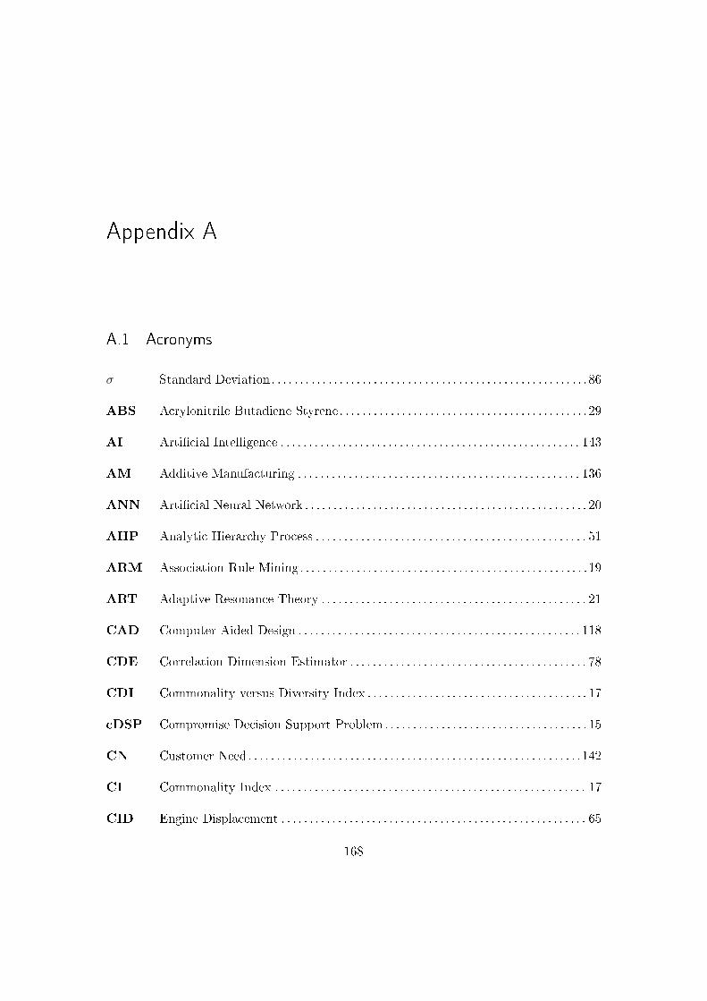
Appendix A
A.1 Acronyms
σ Standard Deviation. . . . . . . . . . . . . . . . . . . . . . . . . . . . . . . . . . . . . . . . . . . . . . . . . . . . . . . .86
ABS Acrylonitrile Butadiene Styrene . . . . . . . . . . . . . . . . . . . . . . . . . . . . . . . . . . . . . . . . . . . .29
AI Arti�cial Intelligence . . . . . . . . . . . . . . . . . . . . . . . . . . . . . . . . . . . . . . . . . . . . . . . . . . . . . 143
AM Additive Manufacturing . . . . . . . . . . . . . . . . . . . . . . . . . . . . . . . . . . . . . . . . . . . . . . . . . . 136
ANN Arti�cial Neural Network . . . . . . . . . . . . . . . . . . . . . . . . . . . . . . . . . . . . . . . . . . . . . . . . . . 20
AHP Analytic Hierarchy Process . . . . . . . . . . . . . . . . . . . . . . . . . . . . . . . . . . . . . . . . . . . . . . . . 51
ARM Association Rule Mining. . . . . . . . . . . . . . . . . . . . . . . . . . . . . . . . . . . . . . . . . . . . . . . . . . .19
ART Adaptive Resonance Theory . . . . . . . . . . . . . . . . . . . . . . . . . . . . . . . . . . . . . . . . . . . . . . . 21
CAD Computer Aided Design . . . . . . . . . . . . . . . . . . . . . . . . . . . . . . . . . . . . . . . . . . . . . . . . . . 118
CDE Correlation Dimension Estimator . . . . . . . . . . . . . . . . . . . . . . . . . . . . . . . . . . . . . . . . . . 78
CDI Commonality versus Diversity Index . . . . . . . . . . . . . . . . . . . . . . . . . . . . . . . . . . . . . . . 17
cDSP Compromise Decision Support Problem . . . . . . . . . . . . . . . . . . . . . . . . . . . . . . . . . . . . 15
CN Customer Need. . . . . . . . . . . . . . . . . . . . . . . . . . . . . . . . . . . . . . . . . . . . . . . . . . . . . . . . . . .142
CI Commonality Index . . . . . . . . . . . . . . . . . . . . . . . . . . . . . . . . . . . . . . . . . . . . . . . . . . . . . . . 17
CID Engine Displacement . . . . . . . . . . . . . . . . . . . . . . . . . . . . . . . . . . . . . . . . . . . . . . . . . . . . . . 65
168
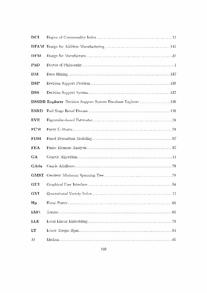
DCI Degree of Commonality Index . . . . . . . . . . . . . . . . . . . . . . . . . . . . . . . . . . . . . . . . . . . . . 17
DFAM Design for Additive Manufacturing . . . . . . . . . . . . . . . . . . . . . . . . . . . . . . . . . . . . . . . 142
DFM Design for Manufacture . . . . . . . . . . . . . . . . . . . . . . . . . . . . . . . . . . . . . . . . . . . . . . . . . . . .31
PhD Doctor of Philosophy . . . . . . . . . . . . . . . . . . . . . . . . . . . . . . . . . . . . . . . . . . . . . . . . . . . . . . . I
DM Data Mining . . . . . . . . . . . . . . . . . . . . . . . . . . . . . . . . . . . . . . . . . . . . . . . . . . . . . . . . . . . . . 137
DSP Decision Support Problem . . . . . . . . . . . . . . . . . . . . . . . . . . . . . . . . . . . . . . . . . . . . . . . . 138
DSS Decision Support System . . . . . . . . . . . . . . . . . . . . . . . . . . . . . . . . . . . . . . . . . . . . . . . . . 137
DSSDB Explorer Decision Support System Database Explorer . . . . . . . . . . . . . . . . . . 139
ESRD End Stage Renal Disease . . . . . . . . . . . . . . . . . . . . . . . . . . . . . . . . . . . . . . . . . . . . . . . . . 116
EVE Eigenvalue-based Estimator. . . . . . . . . . . . . . . . . . . . . . . . . . . . . . . . . . . . . . . . . . . . . . . .78
FCM Fuzzy C-Means . . . . . . . . . . . . . . . . . . . . . . . . . . . . . . . . . . . . . . . . . . . . . . . . . . . . . . . . . . . . 78
FDM Fused Deposition Modeling . . . . . . . . . . . . . . . . . . . . . . . . . . . . . . . . . . . . . . . . . . . . . . . . 97
FEA Finite Element Analysis . . . . . . . . . . . . . . . . . . . . . . . . . . . . . . . . . . . . . . . . . . . . . . . . . . . 97
GA Genetic Algorithm. . . . . . . . . . . . . . . . . . . . . . . . . . . . . . . . . . . . . . . . . . . . . . . . . . . . . . . . .14
GAda Gentle AdaBoost . . . . . . . . . . . . . . . . . . . . . . . . . . . . . . . . . . . . . . . . . . . . . . . . . . . . . . . . . . 79
GMST Geodesic Minimum Spanning Tree . . . . . . . . . . . . . . . . . . . . . . . . . . . . . . . . . . . . . . . . . 78
GUI Graphical User Interface . . . . . . . . . . . . . . . . . . . . . . . . . . . . . . . . . . . . . . . . . . . . . . . . . . . 94
GVI Generational Variety Index . . . . . . . . . . . . . . . . . . . . . . . . . . . . . . . . . . . . . . . . . . . . . . . . 17
Hp Horse Power . . . . . . . . . . . . . . . . . . . . . . . . . . . . . . . . . . . . . . . . . . . . . . . . . . . . . . . . . . . . . . . 65
LbFt Torque . . . . . . . . . . . . . . . . . . . . . . . . . . . . . . . . . . . . . . . . . . . . . . . . . . . . . . . . . . . . . . . . . . . . 65
LLE Local Linear Embedding. . . . . . . . . . . . . . . . . . . . . . . . . . . . . . . . . . . . . . . . . . . . . . . . . . .78
LT Lower Torque Rpm . . . . . . . . . . . . . . . . . . . . . . . . . . . . . . . . . . . . . . . . . . . . . . . . . . . . . . . . 64
M Median . . . . . . . . . . . . . . . . . . . . . . . . . . . . . . . . . . . . . . . . . . . . . . . . . . . . . . . . . . . . . . . . . . . . 85
169
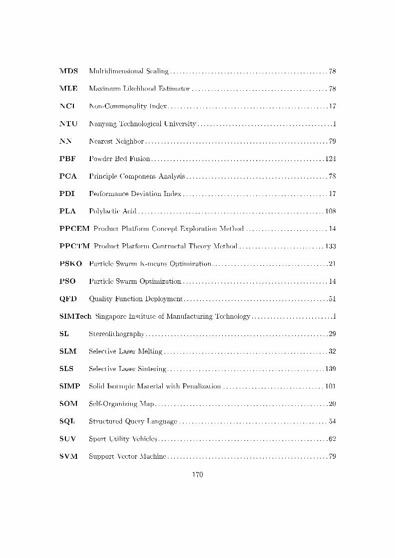
MDS Multidimensional Scaling . . . . . . . . . . . . . . . . . . . . . . . . . . . . . . . . . . . . . . . . . . . . . . . . . . 78
MLE Maximum Likelihood Estimator . . . . . . . . . . . . . . . . . . . . . . . . . . . . . . . . . . . . . . . . . . . 78
NCI Non-Commonality Index. . . . . . . . . . . . . . . . . . . . . . . . . . . . . . . . . . . . . . . . . . . . . . . . . . .17
NTU Nanyang Technological University . . . . . . . . . . . . . . . . . . . . . . . . . . . . . . . . . . . . . . . . . . . I
NN Nearest Neighbor . . . . . . . . . . . . . . . . . . . . . . . . . . . . . . . . . . . . . . . . . . . . . . . . . . . . . . . . . . 79
PBF Powder Bed Fusion . . . . . . . . . . . . . . . . . . . . . . . . . . . . . . . . . . . . . . . . . . . . . . . . . . . . . . . 124
PCA Principle Component Analysis . . . . . . . . . . . . . . . . . . . . . . . . . . . . . . . . . . . . . . . . . . . . . 78
PDI Performance Deviation Index . . . . . . . . . . . . . . . . . . . . . . . . . . . . . . . . . . . . . . . . . . . . . . 17
PLA Polylactic Acid . . . . . . . . . . . . . . . . . . . . . . . . . . . . . . . . . . . . . . . . . . . . . . . . . . . . . . . . . . . 108
PPCEM Product Platform Concept Exploration Method . . . . . . . . . . . . . . . . . . . . . . . . . . 14
PPCTM Product Platform Contructal Theory Method . . . . . . . . . . . . . . . . . . . . . . . . . . . 133
PSKO Particle Swarm K-means Optimization. . . . . . . . . . . . . . . . . . . . . . . . . . . . . . . . . . . . .21
PSO Particle Swarm Optimization . . . . . . . . . . . . . . . . . . . . . . . . . . . . . . . . . . . . . . . . . . . . . . 14
QFD Quality Function Deployment. . . . . . . . . . . . . . . . . . . . . . . . . . . . . . . . . . . . . . . . . . . . . .51
SIMTech Singapore Institute of Manufacturing Technology . . . . . . . . . . . . . . . . . . . . . . . . . . I
SL Stereolithography. . . . . . . . . . . . . . . . . . . . . . . . . . . . . . . . . . . . . . . . . . . . . . . . . . . . . . . . . .29
SLM Selective Laser Melting . . . . . . . . . . . . . . . . . . . . . . . . . . . . . . . . . . . . . . . . . . . . . . . . . . . . 32
SLS Selective Laser Sintering. . . . . . . . . . . . . . . . . . . . . . . . . . . . . . . . . . . . . . . . . . . . . . . . . .139
SIMP Solid Isotropic Material with Penalization . . . . . . . . . . . . . . . . . . . . . . . . . . . . . . . . 101
SOM Self-Organizing Map. . . . . . . . . . . . . . . . . . . . . . . . . . . . . . . . . . . . . . . . . . . . . . . . . . . . . . . 20
SQL Structured Query Language . . . . . . . . . . . . . . . . . . . . . . . . . . . . . . . . . . . . . . . . . . . . . . . 54
SUV Sport Utility Vehicles . . . . . . . . . . . . . . . . . . . . . . . . . . . . . . . . . . . . . . . . . . . . . . . . . . . . . .62
SVM Support Vector Machine . . . . . . . . . . . . . . . . . . . . . . . . . . . . . . . . . . . . . . . . . . . . . . . . . . . 79
170

u-cDSP Utility-Based Compromise Decision Support Problem . . . . . . . . . . . . . . . . . . . . 138
UT Upper Torque Rpm. . . . . . . . . . . . . . . . . . . . . . . . . . . . . . . . . . . . . . . . . . . . . . . . . . . . . . . .64
UV Ultraviolet . . . . . . . . . . . . . . . . . . . . . . . . . . . . . . . . . . . . . . . . . . . . . . . . . . . . . . . . . . . . . . . . 29
171
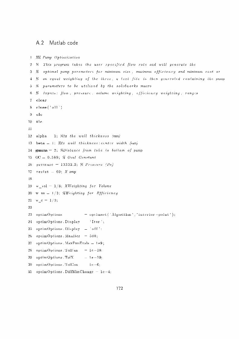
A.2 Matlab code
1 %% Pump Opt imizat ion
2 % This program take s the user s p e c i f i e d f l ow ra t e and w i l l g enera te the
3 % opt imal pump parameters f o r minimum s i z e , maximum e f f i c i e n c y and minimum cos t or
4 % an equa l we i gh t ing o f the three , a t e x t f i l e i s then genera ted con ta in ing the pump
5 % parameters to be u t i l i z e d by the so l i dwor k s macro
6 % Inputs : f low , pressure , volume weigh t ing , e f f i c i e n c y weigh t ing , ranges
7 clear
8 close ( ' a l l ' )
9 clc
10 t ic
11
12 alpha = 1 ; %2x the wa l l t h i c k n e s s (mm)
13 beta = 1 ; %2x wa l l t h i c kn e s s+cen te r width (mm)
14 gamma = 2 ; %Distance from tube to bottom of pump
15 OC = 0 . 5 8 9 ; % Oval Constant
16 pr e s su r e = 13332 . 2 ; % Pressure (Pa)
17 r e s i s t = 60 ; % amp
18
19 w_vol = 1/3 ; %Weighting f o r Volume
20 w_nu = 1/3 ; %Weighting f o r E f f i c i e n c y
21 w_c = 1/3 ;
22
23 optimOptions = opt imset ( ' Algorithm ' , ' i n t e r i o r−point ' ) ;
24 optimOptions . Display = ' I t e r ' ;
25 optimOptions . Display = ' o f f ' ;
26 optimOptions . MaxIter = 500 ;
27 optimOptions . MaxFunEvals = 1e9 ;
28 optimOptions . TolFun = 1e−10;
29 optimOptions . TolX = 1e−10;
30 optimOptions . TolCon = 1e−6;
31 optimOptions . DiffMinChange = 1e−4;
172
32 % optimOptions . PlotFcns = @op t imp lo t f va l ;
33
34 x0 = [ 1 . 8 4 7 8 , 2 . 2 5 4 7 , 4 . 5 1 7 , 0 6 , 0 . 2 1 8 7 ] ; %TW,TH, vo l t ,NoF,FW
35 %x0 = [2 .1021 ,2 . 2345 ,02 . 7264 ,05 , 0 . 3526 ] ; %TW,TH, vo l t ,NoF,FW
36 lb = [ 0 . 5 , 0 . 5 , 0 2 , 0 5 , 0 . 0 ] ;
37 ub = [ 2 . 5 , 3 . 0 , 1 2 , 1 2 , 1 . 0 ] ;
38 n = 1 ;
39 i =1;
40
41 for f low = 100 :50 :600
42
43 %% Optimizat ion f o r min Volume
44 [ x , f , e x i t f l a g , output ] = fmincon (@PumpObjFunc , x0 , [ ] , [ ] , [ ] , [ ] , lb , ub , . . .
45 . . . @PumpCon, optimOptions , alpha , beta ,gamma,OC, f low , pres sure , r e s i s t , w_vol ,w_nu,w_c) ;
46 x (4 ) = round( x ( 4 ) ) ;
47
48 x = f loor ( x * 1000) / 1000 ;
49
50 syms V
51 Voltage = so l v e (x (5)*OC*x (1)* x (2)* x (4 )* ( 9 . 9083*V−6.5144)− f low ) ;
52 x (3 ) = double ( Voltage ) ;
53
54 RPM = 9.9083*x (3)−6.5144;
55 f l owra t e = x (5)*OC*x (1)* x (2)* x (4)*RPM;
56
57 %% Ef f i c i e n c y
58 [ nu , f luid_power , brake_power ] = e f f i c i e n c y ( f l owrate , pres sure , r e s i s t , x ) ;
59 nu ;
60
61 %% Pump Volume
62 [ P_Vol , P_Depth ,P_Width , P_Height ] = PumpVol(x , alpha , beta ,gamma,OC) ;
63 P_Vol ;
64 %% pump cos t
173
65 [P, O, M, L , N, T_B, T_z, T_xy, T_d] = PumpCost (x , alpha , beta ,gamma) ;
66 %f i n g e r pump cos t
67 C = (P + O + M + L)/N;
68
69 %% U t i l i t y
70 U_nu = −6.8238.*nu .^2+5.8722.*nu−0.2650;
71 %U_nu = −1.4323.*nu .^2+2.6802.*nu−0.0381;
72
73 i f U_nu >= 1
74 U_nu = 1 ;
75 end
76 i f U_nu <= 0
77 U_nu = 0 ;
78 end
79 i f nu>=0.45
80 U_nu = 1 ;
81 end
82
83 U_Vol = −1.419*10e−5*P_Vol.^2−8.7807*10 e−4*P_Vol+1.0839
84 i f U_Vol >= 1
85 U_Vol = 1 ;
86 end
87 i f U_Vol <= 0
88 U_Vol = 0 ;
89 end
90 i f P_Vol>=250
91 U_Vol = 0 ;
92 end
93 i f P_Vol <= 50
94 U_Vol = 1 ;
95 end
96
97 U_C = −2.343*10e−6*C^2−3.589*10e−3*C+1.056;
174
98 i f U_C >= 1
99 U_C = 1 ;
100 end
101 i f U_C <= 0
102 U_C = 0 ;
103 end
104 i f C>=150
105 U_C = 0 ;
106 end
107 i f C <= 20
108 U_C = 1 ;
109 end
110
111 x ;
112 U_Vol
113 U_nu
114 U_C
115 U = (1/3*U_nu+1/3*U_Vol+1/3*U_C)
116 Z = 1−U;
117
118 %% Pump Range
119 RPM_Range = [20 , 1 1 2 ] ;
120 flow_range = x (5)*OC*x (1)* x (2)* x (4)*RPM_Range;
121 flow_range = round( flow_range ) ;
122 % x (4) = round ( x ( 4 ) ) ;
123 dim( i , : ) = [ f l owrate , Z , nu , P_Vol , x ( 5 ) , x ( 4 ) , x ( 3 ) , . . .
124 . . . RPM, x (1 ) , x ( 2 ) , U, C, f low , P, O, M, L , N, T_B, T_z, T_xy, T_d ] ;
125 v a r i a b l e s ( i , : ) = [ f l owrate , x ] ;
126 i = i +1;
127
128 end
129 toc
130
175
131 Z_avg = mean(dim ( : , 2 ) )
132 Eff ic_avg = mean(dim ( : , 3 ) )
133 Vol_avg = mean(dim ( : , 4 ) )
134 U_avg = mean(dim ( : , 1 1 ) )
135 C_avg = mean(dim ( : , 1 2 ) )
136
137 f igure
138 plot (dim ( : , 1 3 ) , dim ( : , 1 9 ) , ' o ' )
139 t i t l e ( ' Bui ld time ' )
140 xlabel ( ' Flow Rate ' )
141 ylabel ( 'T_B' )
142 grid on
143
144 f igure
145 plot (dim ( : , 1 3 ) , dim ( : , 1 8 ) , ' o ' )
146 t i t l e ( 'Number o f par t s per bu i ld ' )
147 xlabel ( ' Flow Rate ' )
148 ylabel ( 'N ' )
149 grid on
150
151 f igure
152 plot (dim ( : , 1 3 ) , dim ( : , 1 2 ) , ' o ' )
153 t i t l e ( ' Cost per part ' )
154 xlabel ( ' Flow Rate ' )
155 ylabel ( 'USD ' )
156 grid on
157
158 f igure
159 plot (dim ( : , 1 3 ) , dim ( : , 3 ) , ' o ' )
160 t i t l e ( ' E f f i c i e n c y ' )
161 xlabel ( ' Flow Rate ' )
162 ylabel ( '%' )
163 grid on
176

164
165 f igure
166 plot (dim ( : , 1 3 ) , dim ( : , 4 ) , ' o ' )
167 t i t l e ( 'Volume ' )
168 xlabel ( ' Flow Rate ' )
169 ylabel ( 'cm^3 ' )
170 grid on
Listing A.1: The �nger pump family optimization code.
177