Current Controlled Buck Converter based
Photovoltaic Emulator
Ankur V. Rana C. G. Patel Institute of Technology, Bardoli, Surat, India
Email: [email protected]
Hiren H. Patel Sarvajanik College of Engineering & Technology, Surat, India
Email: [email protected]
Abstract—The output characteristics of the Photovoltaic (PV)
modules, and hence, the array greatly depends on the
environmental factors. Therefore, it is difficult to reproduce
and maintain the same environmental conditions for testing
and comparing the performance of PV power conditioning
systems. A PV emulator, which usually is a power electronic
converter, can reproduce the desired output characteristics
irrespective of the environmental conditions. It gives
opportunity to test and analyze different PV systems in
intended controlled environment. The aim of the work is to
design a current-controlled buck type dc-dc converter based
PV emulator. In order to confirm the effectiveness of the
emulator in reproducing the PV module(s), the performance
of PV emulator is evaluated with different types of loads
(linear and non-linear loads) and is compared with the
results that would have been obtained if the loads were fed
from the real PV source. Extensive simulation results
obtained in MATLAB are included to show that the PV
emulator system behaves electrically similar to a real PV
source.
Index Terms— Photovoltaic, emulator, buck converter
I. INTRODUCTION
Several factors like depletion of the conventional
sources, increase in the cost of electricity, increased
concern about the environment, government policies and
incentives for renewable energy generation, etc. have
drawn more attention of the researchers towards the
renewable or non-conventional energy sources. One of
the most promising renewable energy sources is solar
photovoltaic (PV). Due to number of benefits like direct
solar to electric energy conversion, no operating cost, no
moving parts, modularization, no constraints in terms of
site location etc., the number of PV systems (isolated or
grid-connected) has increased greatly over the past few
years [1]
However, PV systems do have some limitations[2], [3].
These include low efficiency, higher initial cost,
interaction with the other systems connected in parallel,
etc. Also, the effect of the partial shading may lead to
decrease in the output power of the PV array, difficulty in
Manuscript received December 31, 2012; revised January 25, 2013.
tracking the maximum power point (MPP), increase in
harmonics, poor THD etc. Large number of PV systems
in the existing electrical power systems network may also
cause problems like congestion, voltage instability,
resonance etc. Such issues demand investigations in
understanding the behavior of the PV systems. Hence, it
is essential to test such systems prior to their design
and/or installations.
The objective can be achieved with the help of an
experimental set up that is capable of reproducing the
characteristics similar to that of a PV array. Such
experimental set-up is called an emulator [4]-[7]. Some of
the reasons, which suggest the need for an emulator to
reproduce the characteristics of PV array are as under:
The cost of actual PV array is very high.
1) The commissioning of actual PV array requires a
large area. Also, to study the characteristics for
different array configurations one has to reconnect
the PV modules differently, which is a laborious
task and consumes time.
2) It is difficult to emulate a PV array by simply
having either a Current Source (CS) or a Voltage
Source (VS).
3) It gives the liberty to carry out the experimentation
even at the night times when sun is not available or
under cloudy conditions and low insolation
conditions.
4) It is difficult to reproduce and maintain the similar
characteristics with the PV array as the insolation
and other environment conditions do not remain
same.
5) Such emulator can reproduce the different desired
characteristics, within no time and no extra cost, by
just making some minor changes in the algorithm of
the controller.
PV emulators based on op-amp circuits or DC-DC
converters have been proposed over the years [4]-[7]. To
emulate a PV module, a single reference solar cell and a
current amplifier is used as a reference in [7], while Lee
et.al [8], used a look-up-table with discrete values of the
solar panel’s output current and voltage. The system with
solar cell as reference is prone to inaccuracies in case the
solar cells have some defects and/or shading while the
system based on look up table relies on interpolation.
91
Journal of Industrial and Intelligent Information Vol. 1, No. 2, June 2013
©2013 Engineering and Technology Publishingdoi: 10.12720/jiii.1.2.91-96
Also, different look-up tables are required for different
modules. Further, in most of these studies the
performance of the emulator is demonstrated, mostly with
linear resistive load.
The paper presents a current-controlled buck converter
as a PV emulator, which can exhibit the characteristics of
the PV panels. The functioning of the emulator relies on
the PV model[9] and so can emulate different modules
easily with minor modifications. The performance of the
emulator is compared with that of the actual
characteristics and the simulation results are also
presented.
II. PV MODEL
Figure 1. Equivalent Circuit representing a one-diode model of a PV Cell [9]
Fig. 1 shows an equivalent circuit to model a PV cell.
A single diode model is considered [9] along with the
series resistance Rs to take into account the internal
electrical losses. Shunt resistance Rp is generally very
large and hence, ignored. The equation expressing the
relation between output current (Ipv) and its terminal
voltage (Vpv) under given solar radiation (G ) and
temperature (T) is
– ( ( )
) (1)
where,
Io is the diode saturation current [A];
n is the diode quality factor;
q is the electronic charge(1.6 ×10⁻¹⁹
C);
k is the Boltzmann constant (1.6×10⁻²³
J/K);
T is cell temperature [°C];
IL is the photo current generated by PV cell;
The non-linear transcendental equation (1) is difficult
to solve and hence, some numerical technique need to be
used to solve it. The approach suggested by Walker et.al,
[9] is used for solving (1). The characteristic for a
particular module can be obtained using (1)-(8). However,
some data for that module are required, which can be
obtained from the datasheet of the PV module or a priori
from experiments done on the module. Hence, to solve (1)
the previously known values of open circuit voltage (Voc)
and short circuit current (Isc) at two different temperatures
T1 and T2 are used. The subscript ‘1’ and ‘nom’ refers to
the standard conditions (Gnom = 1000W/m2, T1 = 25°C).
( ) ( ⁄ )
((
) (
–
))
(2)
( ) ( )
( ( )
– )
⁄ (3)
where, Vg is the energy gap of the material of the cell.
( ) ( ( ) ) (4)
( ) ( ) ( )⁄ (5)
( ( ) ( ) )
( )⁄ (6)
where Ko is the temperature coefficient of Isc (A/K). The
series resistance is computed using following equations
⁄ (7)
( ) ⁄
( )
(8)
III. SYSTEM CONFIGURATION
Fig. 2 shows the system configuration for a PV
emulator which comprises a buck type (step-down) dc-dc
converter, sensors, conditioning circuits, controller a gate
drive circuit. Vin represents a DC source of 100V.
Hysteresis (or bang-bang) control is used to provide
controlled output current. The reference current for the
hysteresis controller is derived using the PV model. The
value of inductor L and filter capacitor C are 25mH and
2000µF, respectively.
Figure 2. System configuration of a PV emulator
As shown in Fig. 2, the output voltage Vo and the
output current Io of the converter are sensed, filtered and
fed to the controller, which controls the converter to
behave like a PV module i.e. to act as a PV emulator. It is
evident that a PV module (or an array) operates at
different values of Vpv and Ipv depending on values of G,
T and the load connected across it (Rload). Hence, to
control the buck converter to operate at the voltage and
current in accordance to the values at which a PV
module operate under given conditions, the controller is
fed with G, T, Vo and Io. The controller employs the PV
model discussed in Section II. Using (1)-(8) and the
parameters G,T, Vo and Io, the controller computes the
value of Rpv and Rload. Rpv is defined as the ratio of Vpv and
Ipv. Depending on the difference in the value of Rload and
Rpv, the controller takes the corrective action to force the
operating point where, difference in Rload and Rpv is zero
or is negligible. The operating principle and the algorithm
for controlling the dc-dc converter as the PV emulator, is
discussed in the next section.
IV. ALGORITHM FOR THE CONTROL OF CONVERTER
G
T
Io
RSIpv
Vpv
IL
Voltage
conditioning
Circuit
Current Sensing
& Conditioning
Circuit
PV
MODEL
Vo / Io
TG
Bang – Bang
Control
Gate
Drive
L Io
Vo
Iref
Vin
Load
Io
Vo
Io
Rload
Vo
C
DSP Implementation
92
Journal of Industrial and Intelligent Information Vol. 1, No. 2, June 2013
©2013 Engineering and Technology Publishing
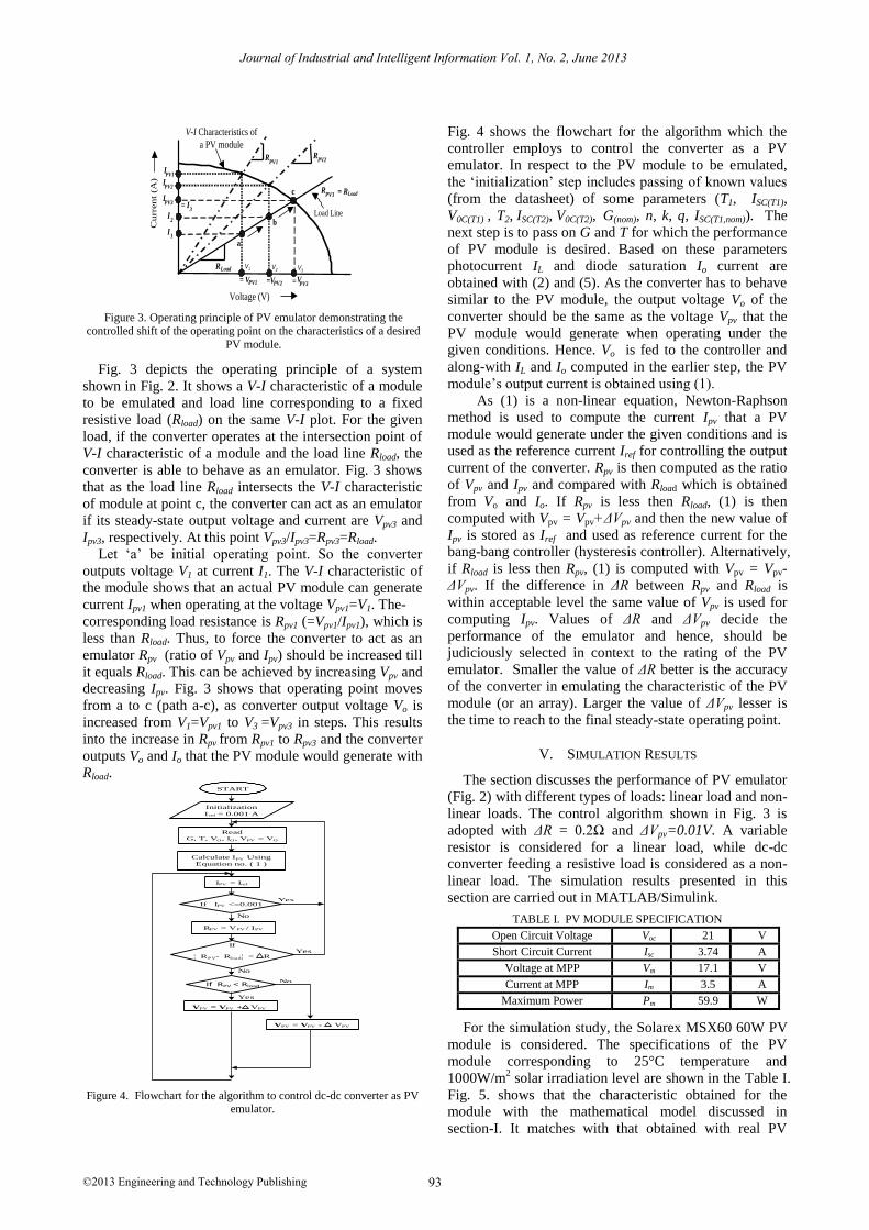
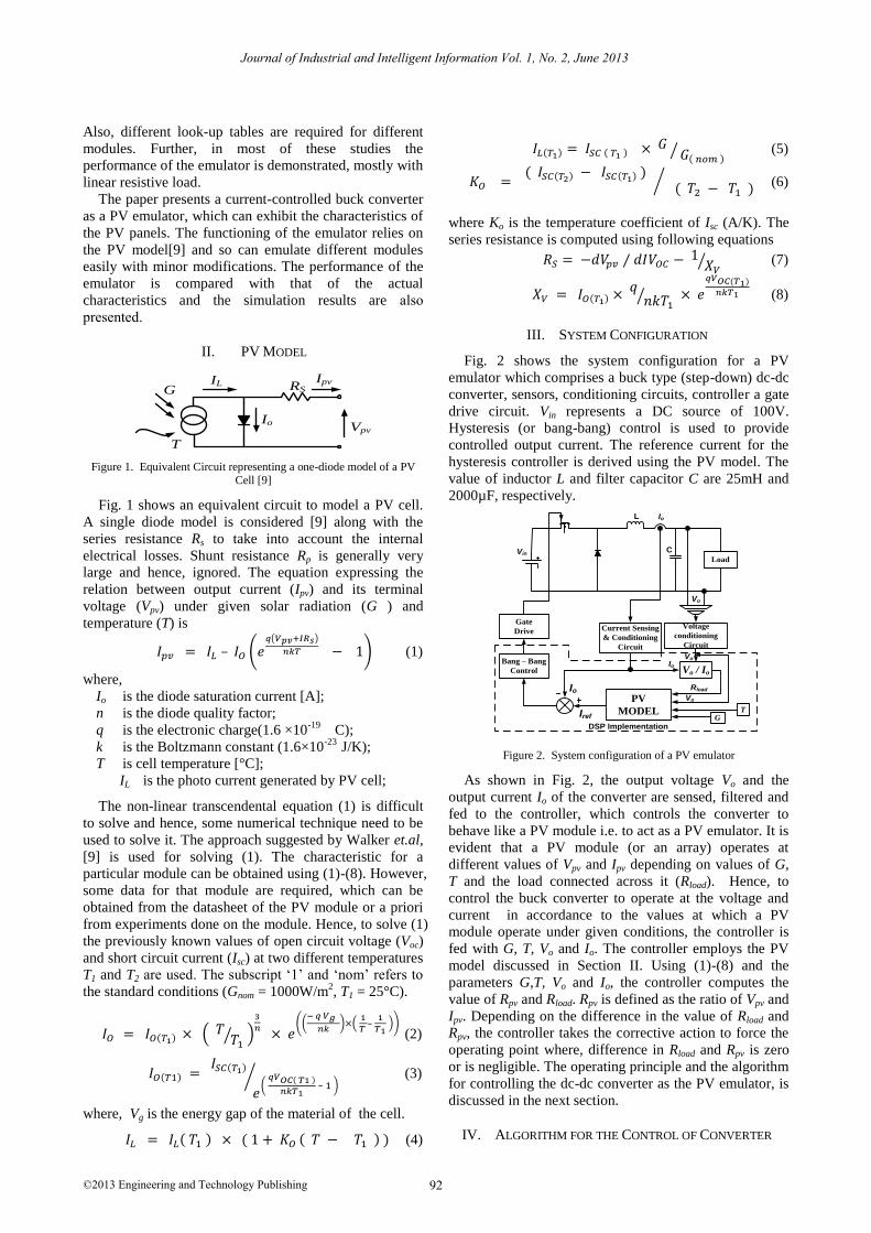
Figure 3. Operating principle of PV emulator demonstrating the controlled shift of the operating point on the characteristics of a desired
PV module.
Fig. 3 depicts the operating principle of a system
shown in Fig. 2. It shows a V-I characteristic of a module
to be emulated and load line corresponding to a fixed
resistive load (Rload) on the same V-I plot. For the given
load, if the converter operates at the intersection point of
V-I characteristic of a module and the load line Rload, the
converter is able to behave as an emulator. Fig. 3 shows
that as the load line Rload intersects the V-I characteristic
of module at point c, the converter can act as an emulator
if its steady-state output voltage and current are Vpv3 and
Ipv3, respectively. At this point Vpv3/Ipv3=Rpv3=Rload.
Let ‘a’ be initial operating point. So the converter
outputs voltage V1 at current I1. The V-I characteristic of
the module shows that an actual PV module can generate
current Ipv1 when operating at the voltage Vpv1=V1. The-
corresponding load resistance is Rpv1 (=Vpv1/Ipv1), which is
less than Rload. Thus, to force the converter to act as an
emulator Rpv (ratio of Vpv and Ipv) should be increased till
it equals Rload. This can be achieved by increasing Vpv and
decreasing Ipv. Fig. 3 shows that operating point moves
from a to c (path a-c), as converter output voltage Vo is
increased from V1=Vpv1 to V3 =Vpv3 in steps. This results
into the increase in Rpv from Rpv1 to Rpv3 and the converter
outputs Vo and Io that the PV module would generate with
Rload.
Figure 4. Flowchart for the algorithm to control dc-dc converter as PV emulator.
Fig. 4 shows the flowchart for the algorithm which the
controller employs to control the converter as a PV
emulator. In respect to the PV module to be emulated,
the ‘initialization’ step includes passing of known values
(from the datasheet) of some parameters (T1, ISC(T1),
V0C(T1) , T2, ISC(T2), V0C(T2), G(nom), n, k, q, ISC(T1,nom)). The
next step is to pass on G and T for which the performance
of PV module is desired. Based on these parameters
photocurrent IL and diode saturation Io current are
obtained with (2) and (5). As the converter has to behave
similar to the PV module, the output voltage Vo of the
converter should be the same as the voltage Vpv that the
PV module would generate when operating under the
given conditions. Hence. Vo is fed to the controller and
along-with IL and Io computed in the earlier step, the PV
module’s output current is obtained using (1).
As (1) is a non-linear equation, Newton-Raphson
method is used to compute the current Ipv that a PV
module would generate under the given conditions and is
used as the reference current Iref for controlling the output
current of the converter. Rpv is then computed as the ratio
of Vpv and Ipv and compared with Rload which is obtained
from Vo and Io. If Rpv is less then Rload, (1) is then
computed with Vpv = Vpv+ΔVpv and then the new value of
Ipv is stored as Iref and used as reference current for the
bang-bang controller (hysteresis controller). Alternatively,
if Rload is less then Rpv, (1) is computed with Vpv = Vpv-
ΔVpv. If the difference in ΔR between Rpv and Rload is
within acceptable level the same value of Vpv is used for
computing Ipv. Values of ΔR and ΔVpv decide the
performance of the emulator and hence, should be
judiciously selected in context to the rating of the PV
emulator. Smaller the value of ΔR better is the accuracy
of the converter in emulating the characteristic of the PV
module (or an array). Larger the value of ΔVpv lesser is
the time to reach to the final steady-state operating point.
V. SIMULATION RESULTS
The section discusses the performance of PV emulator
(Fig. 2) with different types of loads: linear load and non-
linear loads. The control algorithm shown in Fig. 3 is
adopted with ΔR = 0.2Ω and ΔVpv=0.01V. A variable
resistor is considered for a linear load, while dc-dc
converter feeding a resistive load is considered as a non-
linear load. The simulation results presented in this
section are carried out in MATLAB/Simulink.
TABLE I. PV MODULE SPECIFICATION
Open Circuit Voltage Voc 21 V
Short Circuit Current Isc 3.74 A
Voltage at MPP Vm 17.1 V
Current at MPP Im 3.5 A
Maximum Power Pm 59.9 W
For the simulation study, the Solarex MSX60 60W PV
module is considered. The specifications of the PV
module corresponding to 25°C temperature and
1000W/m2 solar irradiation level are shown in the Table I.
Fig. 5. shows that the characteristic obtained for the
module with the mathematical model discussed in
section-I. It matches with that obtained with real PV
V-I Characteristics of
a PV module
a
bLoad Line
R Load
= VPV1 =
V1
c
VPV2
V2
= PV3
V3
V
PV1I
PV2I
PV3I
PV1R PV2
R
PV3R = RLoad
Voltage (V)
Cu
rrent
(A)
1I
2I
3= I
START
ReadG, T, VO, IO, VPV = VO
Calculate IPV Using
Equation no. ( 1 )
IPV = Iref
RPV = VPV / IPV
VPV = VPV + VPV
VPV = VPV - VPV
Initialization
I ref = 0.001 A
If IPV <=0.001
If
¦RPV- Rload¦< ? R
If RPV < Rload
No
No
Yes
Yes
Yes
No
93
Journal of Industrial and Intelligent Information Vol. 1, No. 2, June 2013
©2013 Engineering and Technology Publishing
model. It is observed that the characteristic is non-linear
and is difficult to obtain it by just a CS or a VS.
Figure 5. V-I characteristics of PV Module
The operating point on the characteristic; may it be on
CS region, non-linear region, or VS region; is dependent
on the load. If Rload =R =10Ω, the operation will be at a
point where the PV module’s output voltage and current
are such that their ratio is equal to 10Ω. This is achieved
at point C, where the output voltage and current are
19.69V and 1.969A, respectively (19.69/1.969=10Ω).
Thus, depending on the load matching, there exists a
unique point on the characteristic where the operation is
possible. Hence, as the Rload changes, the output voltage
and current of the PV array change, unlike an ideal CS or
a VS where only one of these either output voltage or
output current changes. Some reference points A
(R=2.63Ω), B (R=5Ω), C(R=10Ω) and D(R=50Ω) are
marked, which shows that the Rpv decreases as the
operation moves from Point A (in the VS region),
towards the point D (in the CS region).
Figure 6. PV emulator response when feeding a resistive load: (a) Output voltage (b) Output current and (c) output voltage versus output
current
Fig. 6 shows performance of the PV emulator (Fig. 2),
when the resistance is varied (corresponding to points A`
to D`). Rload at time t=0s is 2.63Ω . The step change in the
resistances are applied at t=0.05s (2.63Ω to 5Ω), t=0.1s
(5Ω to 10Ω), and t=0.15s (10Ω to 50Ω). Fig. 6(a) and (b)
show the variation in the dc-dc converter’s output voltage
and current respectively, corresponding to these
resistances. The steady state operating points (A`B`C`D`)
obtained with the PV emulator are also highlighted in Fig.
6(c). It can be observed from Figs. 5 and Figs. 6(c) that
the steady state operating points for both the cases; (i)
resistive load directly fed from PV module (Fig. 5) and (ii)
resistive load fed from the converter (Fig. 6(c)); have a
close match. Thus, the dc-dc buck converter is controlled
as a PV emulator to behave similar to that of the PV
module. The response time of the emulator when a step
change in resistance is applied is also very small, less
than 0.01s. Unlike the results shown in Fig. 5, ripple in Io
(about 0.1A) and Vo (about 0.0007V) is observed in Fig.
6.However, the ripple is quite small and has not much
significance when the PV emulator is used in place of PV
module for testing the PV systems. In fact, the ripple in Io
and Vo can be minimized, if desired, by increasing the
buck inductance and filter capacitance.
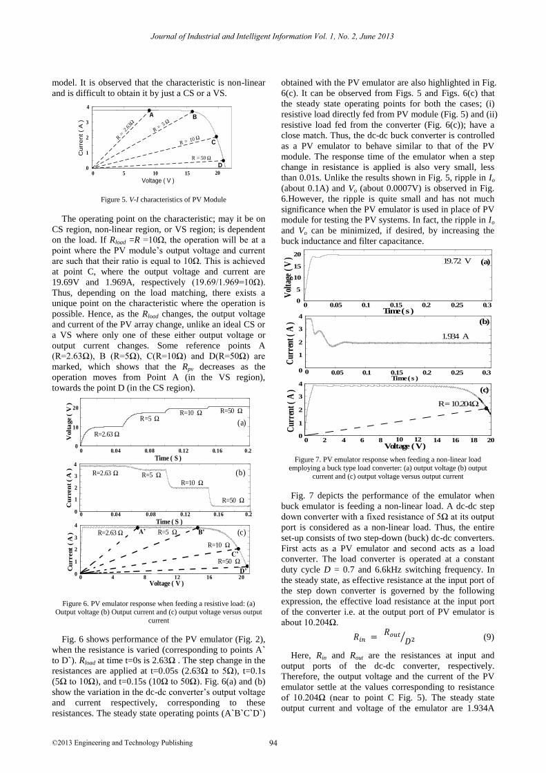
Figure 7. PV emulator response when feeding a non-linear load
employing a buck type load converter: (a) output voltage (b) output current and (c) output voltage versus output current
Fig. 7 depicts the performance of the emulator when
buck emulator is feeding a non-linear load. A dc-dc step
down converter with a fixed resistance of 5Ω at its output
port is considered as a non-linear load. Thus, the entire
set-up consists of two step-down (buck) dc-dc converters.
First acts as a PV emulator and second acts as a load
converter. The load converter is operated at a constant
duty cycle D = 0.7 and 6.6kHz switching frequency. In
the steady state, as effective resistance at the input port of
the step down converter is governed by the following
expression, the effective load resistance at the input port
of the converter i.e. at the output port of PV emulator is
about 10.204Ω.
⁄ (9)
Here, Rin and Rout are the resistances at input and
output ports of the dc-dc converter, respectively.
Therefore, the output voltage and the current of the PV
emulator settle at the values corresponding to resistance
of 10.204Ω (near to point C Fig. 5). The steady state
output current and voltage of the emulator are 1.934A
Cu
rre
nt (
A )
0 5 10 150
1
2
3
4
20
A B
C
D
R = 2
.63Ω
R = 50 Ω
R = 5
Ω
R = 10 Ω
Voltage ( V )
Cu
rre
nt
( A
) R=2.63 Ω
0 0.04 0.08 0.12 0.16 0.20
10
20
Time ( S )
Volt
age (
V )
0 0.04 0.08 0.12 0.16 0.20
1
2
3
4
Time ( S )
0 4 8 12 16 200
1
2
3
4
Voltage ( V )
Cu
rrent
( A
)
R=2.63 Ω
R=5 ΩR=10 Ω R=50 Ω
R=5 ΩR=10 Ω
R=50 Ω
R=2.63 Ω R=5 Ω
R=10 Ω
R=50 Ω
(a)
(b)
(c)A’ B’
C’
D’
0 0.05 0.1 0.15 0.2 0.25 0.30
5
10
15
20
Time ( s )
Vol
tage
( V
)
0 0.05 0.1 0.15 0.2 0.25 0.30
1
2
3
4
Time ( s )
Cur
rent
( A
)
0 2 4 6 8 10 12 14 16 18 200
1
2
3
4
Voltage ( V )
Cur
rent
( A
)
19.72 V
1.934 A
R = 10.204Ω
(a)
(b)
(c)
94
Journal of Industrial and Intelligent Information Vol. 1, No. 2, June 2013
©2013 Engineering and Technology Publishing
19.72V, respectively, which is in accordance to the output
of the PV module as observed from Fig. 5. Ripple in the
output current is about 0.1A and that in output voltage is
0.004V. The time to reach the steady state is 0.07s. As
the duty cycle of this converter varies, the effective
resistance at the input port of the converter varies
yielding different operating point on the V-I
characteristics of Fig. 5. Though the performance is not
shown for other values of duty cycles, the performance of
PV emulator for different duty cycles is in agreement
with that obtained when the non-linear load is directly
connected to the PV module.
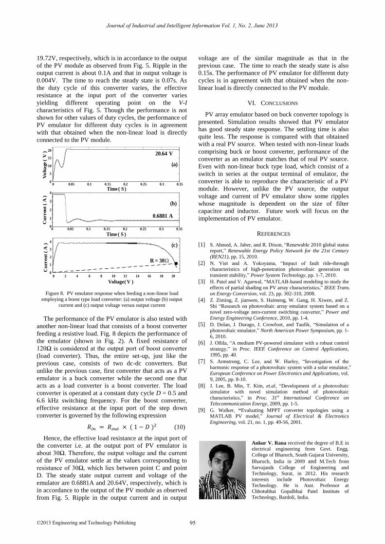
Figure 8. PV emulator response when feeding a non-linear load employing a boost type load converter: (a) output voltage (b) output
current and (c) output voltage versus output current
The performance of the PV emulator is also tested with
another non-linear load that consists of a boost converter
feeding a resistive load. Fig. 8 depicts the performance of
the emulator (shown in Fig. 2). A fixed resistance of
120Ω is considered at the output port of boost converter
(load converter). Thus, the entire set-up, just like the
previous case, consists of two dc-dc converters. But
unlike the previous case, first converter that acts as a PV
emulator is a buck converter while the second one that
acts as a load converter is a boost converter. The load
converter is operated at a constant duty cycle D = 0.5 and
6.6 kHz switching frequency. For the boost converter,
effective resistance at the input port of the step down
converter is governed by the following expression
( ) (10)
Hence, the effective load resistance at the input port of
the converter i.e. at the output port of PV emulator is
about 30Ω. Therefore, the output voltage and the current
of the PV emulator settle at the values corresponding to
resistance of 30Ω, which lies between point C and point
D. The steady state output current and voltage of the
emulator are 0.6881A and 20.64V, respectively, which is
in accordance to the output of the PV module as observed
from Fig. 5. Ripple in the output current and in output
voltage are of the similar magnitude as that in the
previous case. The time to reach the steady state is also
0.15s. The performance of PV emulator for different duty
cycles is in agreement with that obtained when the non-
linear load is directly connected to the PV module.
VI. CONCLUSIONS
PV array emulator based on buck converter topology is
presented. Simulation results showed that PV emulator
has good steady state response. The settling time is also
quite less. The response is compared with that obtained
with a real PV source. When tested with non-linear loads
comprising buck or boost converter, performance of the
converter as an emulator matches that of real PV source.
Even with non-linear buck type load, which consist of a
switch in series at the output terminal of emulator, the
converter is able to reproduce the characteristic of a PV
module. However, unlike the PV source, the output
voltage and current of PV emulator show some ripples
whose magnitude is dependent on the size of filter
capacitor and inductor. Future work will focus on the
implementation of PV emulator.
REFERENCES
[1] S. Ahmed, A. Jaber, and R. Dixon, “Renewable 2010 global status report,” Renewable Energy Policy Network for the 21st Century
(REN21), pp. 15, 2010. [2] N. Viet and A. Yokoyama, “Impact of fault ride-through
characteristics of high-penetration photovoltaic generation on
transient stability,” Power System Technology, pp. 1-7, 2010. [3] H. Patel and V. Agarwal, “MATLAB-based modeling to study the
effects of partial shading on PV array characteristics,” IEEE Trans.
on Energy Conversion, vol. 23, pp. 302-310, 2008. [4] Z. Ziming, Z. jianwen, S. Haimeng, W. Gang, H. Xiwen, and Z.
Shi “Research on photovoltaic array emulator system based on a novel zero-voltage zero-current switching converter,” Power and
Energy Engineering Conference, 2010, pp. 1-4.
[5] D. Dolan, J. Durago, J. Crowfoot, and Taufik, “Simulation of a photovoltaic emulator,” North American Power Symposium, pp. 1-
6, 2010. [6] J. Ollila, “A medium PV-powered simulator with a robust control
strategy,” in Proc. IEEE Conference on Control Applications, 1995, pp. 40.
[7] S. Armstrong, C. Lee, and W. Hurley, “Investigation of the
harmonic response of a photovoltaic system with a solar emulator,”
European Conference on Power Electronics and Applications, vol.
9, 2005, pp. 8-10.
[8] J. Lee, B. Min, T. Kim, et.al, “Development of a photovoltaic simulator with novel simulation method of photovoltaic
characteristics,” in Proc. 31st International Conference on Telecommunication Energy, 2009, pp. 1-5.
[9] G. Walker, “Evaluating MPPT converter topologies using a MATLAB PV model,” Journal of Electrical & Electronics
Engineering, vol. 21, no. 1, pp. 49-56, 2001.
Ankur V. Rana received the degree of B.E in
electrical engineering from Govt. Engg.
College of Bharuch, South Gujarat University,
Bharuch, India in 2009 and M.Tech from
Sarvajanik College of Engineering and Technology, Surat, in 2012. His research
interests include Photovoltaic Energy
Technology. He is Asst. Professor at Chhotubhai Gopalbhai Patel Institute of
Technology, Bardoli, India.
0 2 4 6 8 10 12 14 16 18 200
1
2
3
4
Voltage( V )
Cu
rren
t(
A)
20.64 V
0.6881 A
R = 30
(a)
(b)
(c)
Time ( S )0 0.05 0.1 0.15 0.2 0.25 0.3 0.35
0
1
2
3
4
Cu
rren
t(
A)
0 0.05 0.1 0.15 0.2 0.25 0.3 0.350
5
10
15
20
Time ( S )
Vo
lta
ge
(V
)
95
Journal of Industrial and Intelligent Information Vol. 1, No. 2, June 2013
©2013 Engineering and Technology Publishing

Hiren H. Patel received the degree of B.E in electrical engineering from S.V. National
Institute of Technology, South Gujarat
University, Surat, India in 1996 and M.Tech and Ph.D degrees from Indian Institute of
Technology, Bombay, India, in 2003 and
2009, respectively. His research interests include computer-aided simulation
techniques, distributed generation, and
renewable energy, especially energy extraction from photovoltaic arrays. He is Professor at Sarvajanik
College of Engineering and Technology, Surat, India and is a certified
energy manager. He has authored several international and national research papers and is a life member of Indian Society for Technical
Education.
96
Journal of Industrial and Intelligent Information Vol. 1, No. 2, June 2013
©2013 Engineering and Technology Publishing