DG-05603-001_v4.1 | January 2012
Design Guide
CUDA C BEST PRACTICES GUIDE
www.nvidia.com
CUDA C Best Practices Guide DG-05603-001_v4.1 | ii
DOCUMENT CHANGE HISTORY
DG-05603-001_v4.1
Version Date Authors Description of Change
3.0 February 4, 2010 CW
3.1 May 19, 2010 CW
3.2 August 20, 2010 CW
4.0 May 9, 2011 CW,NJ,VS
4.1 January 11, 2012 CW,TB,JV,GZ See Section C.1
www.nvidia.com
CUDA C Best Practices Guide DG-05603-001_v4.1 | iii
TABLE OF CONTENTS
PREFACE ......................................................................................................... 1
What is This Document? ..................................................................................... 1
Who Should Read This Guide? .............................................................................. 1
Assess, Parallelize, Optimize, Deploy ...................................................................... 2
Assess ....................................................................................................... 3
Parallelize ................................................................................................... 3
Optimize ..................................................................................................... 3
Deploy ....................................................................................................... 4
Recommendations and Best Practices ..................................................................... 4
ASSESSING YOUR APPLICATION ........................................................................ 5
Chapter 1. Heterogeneous Computing .................................................................... 6
1.1 Differences Between Host and Device.............................................................. 6
1.2 What Runs on a CUDA-Enabled Device? ........................................................... 7
Chapter 2. Application Profiling ....................................................................... 9
2.1 Profile .................................................................................................... 9
2.1.1 Creating the Profile ............................................................................ 9
2.1.2 Identifying Hotspots ......................................................................... 10
2.1.3 Understanding Scaling ....................................................................... 10
PARALLELIZING YOUR APPLICATION ........................................................................ 13
Chapter 3. Getting Started ............................................................................ 14
3.1 Parallel Libraries....................................................................................... 14
3.2 Parallelizing Compilers ............................................................................... 15
3.3 Coding to Expose Parallelism ....................................................................... 15
Chapter 4. Getting The Right Answer ............................................................. 16
4.1 Verification ............................................................................................. 16
4.1.1 Reference Comparison ....................................................................... 16
4.1.2 Unit Testing ................................................................................... 17
4.2 Debugging ............................................................................................. 17
4.3 Numerical Accuracy and Precision ................................................................. 18
4.3.1 Single vs. Double Precision ................................................................. 18
4.3.2 Floating-Point Math Is Not Associative .................................................... 18
4.3.3 Promotions to Doubles and Truncations to Floats ...................................... 18
4.3.4 IEEE 754 Compliance ........................................................................ 19
4.3.5 x86 80-bit Computations .................................................................... 19
OPTIMIZING CUDA APPLICATIONS................................................................... 20
Chapter 5. Performance Metrics .................................................................... 21
5.1 Timing .................................................................................................. 21
5.1.1 Using CPU Timers ............................................................................ 21
5.1.2 Using CUDA GPU Timers .................................................................... 22
5.2 Bandwidth .............................................................................................. 23
5.2.1 Theoretical Bandwidth Calculation ......................................................... 23
www.nvidia.com
CUDA C Best Practices Guide DG-05603-001_v4.1 | iv
5.2.2 Effective Bandwidth Calculation ............................................................ 23
5.2.3 Throughput Reported by Visual Profiler................................................... 24
Chapter 6. Memory Optimizations .................................................................. 25
6.1 Data Transfer Between Host and Device ......................................................... 25
6.1.1 Pinned Memory ............................................................................... 26
6.1.2 Asynchronous Transfers and Overlapping Transfers with Computation ............. 26
6.1.3 Zero Copy ...................................................................................... 29
6.1.4 Unified Virtual Addressing ................................................................... 30
6.2 Device Memory Spaces .............................................................................. 30
6.2.1 Coalesced Access to Global Memory ...................................................... 32
6.2.2 Shared Memory ............................................................................... 37
6.2.3 Local Memory ................................................................................. 44
6.2.4 Texture Memory .............................................................................. 45
6.2.5 Constant Memory ............................................................................. 46
6.2.6 Registers ....................................................................................... 46
6.3 Allocation ............................................................................................... 47
Chapter 7. Execution Configuration Optimizations ........................................... 48
7.1 Occupancy ............................................................................................. 48
7.1.1 Calculating Occupancy ....................................................................... 49
7.2 Hiding Register Dependencies ...................................................................... 50
7.3 Thread and Block Heuristics ........................................................................ 51
7.4 Effects of Shared Memory ........................................................................... 52
Chapter 8. Instruction Optimizations ............................................................. 54
8.1 Arithmetic Instructions ............................................................................... 54
8.1.1 Division and Modulo Operations ........................................................... 54
8.1.2 Reciprocal Square Root ...................................................................... 55
8.1.3 Other Arithmetic Instructions ............................................................... 55
8.1.4 Math Libraries ................................................................................. 55
8.1.5 Precision-related Compiler Flags ........................................................... 57
8.2 Memory Instructions ................................................................................. 57
Chapter 9. Control Flow ............................................................................... 58
9.1 Branching and Divergence .......................................................................... 58
9.2 Branch Predication .................................................................................... 59
9.3 Loop counters signed vs. unsigned ................................................................ 59
DEPLOYING CUDA APPLICATIONS .................................................................... 61
Chapter 10. Understanding the Programming Environment .............................. 62
10.1 CUDA Compute Capability ......................................................................... 62
10.2 Additional Hardware Data ......................................................................... 63
10.3 CUDA Runtime and Driver API Version .......................................................... 63
10.4 Which Compute Capability to Target ............................................................ 64
10.5 CUDA Runtime ...................................................................................... 65
Chapter 11. Preparing the Application for Deployment .................................... 66
11.1 Error handling ....................................................................................... 66
11.2 Distributing the CUDA Runtime and libraries ................................................... 66
Chapter 12. Deployment Infrastructure Tools ................................................ 68
www.nvidia.com
CUDA C Best Practices Guide DG-05603-001_v4.1 | v
12.1 nvidia-smi ............................................................................................ 68
12.1.1 Queryable state ............................................................................... 68
12.1.2 Modifiable state ............................................................................... 69
12.2 NVML ................................................................................................. 69
12.3 Cluster Management Tools ........................................................................ 70
12.4 Compiler JIT Cache Management ................................................................ 70
12.5 CUDA_VISIBLE_DEVICES.......................................................................... 70
Appendix A. Recommendations and Best Practices .......................................... 71
A.1 Overall Performance Optimization Strategies .................................................. 71
Appendix B. NVCC Compiler Switches ............................................................ 73
B.1 NVCC ................................................................................................. 73
Appendix C. Revision History ....................................................................... 74
C.1 Version 4.1........................................................................................... 74
www.nvidia.com
CUDA C Best Practices Guide DG-05603-001_v4.1 | 1
PREFACE
WHAT IS THIS DOCUMENT?
This Best Practices Guide is a manual to help developers obtain the best performance
from the NVIDIA® CUDA™ architecture using version 4.1 of the CUDA Toolkit. It
presents established parallelization and optimization techniques and explains coding
metaphors and idioms that can greatly simplify programming for the CUDA
architecture.
While the contents can be used as a reference manual, you should be aware that some
topics are revisited in different contexts as various programming and configuration
topics are explored. As a result, it is recommended that first-time readers proceed
through the guide sequentially. This approach will greatly improve your understanding
of effective programming practices and enable you to better use the guide for reference
later.
WHO SHOULD READ THIS GUIDE?
The discussions in this guide all use the C programming language, so you should be
comfortable reading C code.
This guide refers to and relies on several other documents that you should have at your
disposal for reference, all of which are available at no cost from the CUDA website
http://developer.nvidia.com/cuda-downloads. The following documents are especially
important resources:
CUDA Getting Started Guide
CUDA C Programming Guide
Heterogeneous Computing
www.nvidia.com
CUDA C Best Practices Guide DG-05603-001_v4.1 | 2
CUDA Toolkit Reference Manual
In particular, the optimization section of this guide assumes that you have already
successfully downloaded and installed the CUDA Toolkit (if not, please refer to the
relevant CUDA Getting Started Guide for your platform) and that you have a basic
familiarity with the CUDA C programming language and environment (if not, please
refer to the CUDA C Programming Guide).
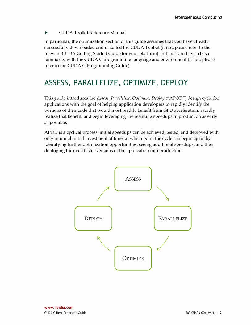
ASSESS, PARALLELIZE, OPTIMIZE, DEPLOY
This guide introduces the Assess, Parallelize, Optimize, Deploy (“APOD”) design cycle for
applications with the goal of helping application developers to rapidly identify the
portions of their code that would most readily benefit from GPU acceleration, rapidly
realize that benefit, and begin leveraging the resulting speedups in production as early
as possible.
APOD is a cyclical process: initial speedups can be achieved, tested, and deployed with
only minimal initial investment of time, at which point the cycle can begin again by
identifying further optimization opportunities, seeing additional speedups, and then
deploying the even faster versions of the application into production.
ASSESS
PARALLELIZE
OPTIMIZE
DEPLOY

Heterogeneous Computing
www.nvidia.com
CUDA C Best Practices Guide DG-05603-001_v4.1 | 3
Assess
For an existing project, the first step is to assess the application to locate the parts of the
code that are responsible for the bulk of the execution time. Armed with this knowledge,
the developer can evaluate these bottlenecks for parallelization and start to investigate
GPU acceleration.
By understanding the end-user’s requirements and constraints and by applying
Amdahl’s and Gustafson’s laws, the developer can determine the upper bound of
performance improvement from acceleration of the identified portions of the
application.
Parallelize
Having identified the hotspots and having done the basic exercises to set goals and
expectations, the developer needs to parallelize the code. Depending on the original
code, this can be as simple as calling into an existing GPU-optimized library such as
cuBLAS, cuFFT, or Thrust, or it could be as simple as adding a few preprocessor
directives as hints to a parallelizing compiler.
On the other hand, some applications’ designs will require some amount of refactoring
to expose their inherent parallelism. As even future CPU architectures will require
exposing this parallelism in order to improve or simply maintain the performance of
sequential applications, the CUDA family of parallel programming languages (CUDA
C/C++, CUDA Fortran, etc.) aims to make the expression of this parallelism as simple as
possible, while simultaneously enabling operation on CUDA-capable GPUs designed for
maximum parallel throughput.
Optimize
After each round of application parallelization is complete, the developer can move to
optimizing the implementation to improve performance. Since there are many possible
optimizations that can be considered, having a good understanding of the needs of the
application can help to make the process as smooth as possible. However, as with APOD
as a whole, program optimization is an iterative process (identify an opportunity for
optimization, apply and test the optimization, verify the speedup achieved, and repeat),
meaning that it is not necessary for a programmer to spend large amounts of time
memorizing the bulk of all possible optimization strategies prior to seeing good
speedups. Instead, strategies can be applied incrementally as they are learned.
Optimizations can be applied at various levels, from overlapping data transfers with
computation all the way down to fine-tuning floating-point operation sequences. The
available profiling tools are invaluable for guiding this process, as they can help suggest
a next-best course of action for the developer’s optimization efforts and provide
references into the relevant portions of the optimization section of this guide.

Heterogeneous Computing
www.nvidia.com
CUDA C Best Practices Guide DG-05603-001_v4.1 | 4
Deploy
Having completed the GPU acceleration of one or more components of the application it
is possible to compare the outcome with the original expectation. Recall that the initial
assess step allowed the developer to determine an upper bound for the potential
speedup attainable by accelerating given hotspots.
Before tackling other hotspots to improve the total speedup, the developer should
consider taking the partially parallelized implementation and carry it through to
production. This is important for a number of reasons; for example, it allows the user to
profit from their investment as early as possible (the speedup may be partial but is still
valuable), and it minimizes risk for the developer and the user by providing an
evolutionary rather than revolutionary set of changes to the application.
RECOMMENDATIONS AND BEST PRACTICES
Throughout this guide, specific recommendations are made regarding the design and
implementation of CUDA C code. These recommendations are categorized by priority,
which is a blend of the effect of the recommendation and its scope. Actions that present
substantial improvements for most CUDA applications have the highest priority, while
small optimizations that affect only very specific situations are given a lower priority.
Before implementing lower priority recommendations, it is good practice to make sure
all higher priority recommendations that are relevant have already been applied. This
approach will tend to provide the best results for the time invested and will avoid the
trap of premature optimization.
The criteria of benefit and scope for establishing priority will vary depending on the
nature of the program. In this guide, they represent a typical case. Your code might
reflect different priority factors. Regardless of this possibility, it is good practice to verify
that no higher-priority recommendations have been overlooked before undertaking
lower-priority items.
Code samples throughout the guide omit error checking for conciseness. Production
code should, however, systematically check the error code returned by each API call and
check for failures in kernel launches by calling cudaGetLastError().

www.nvidia.com
CUDA C Best Practices Guide DG-05603-001_v4.1 | 5
ASSESSING YOUR APPLICATION
From supercomputers to mobile phones, modern processors increasingly rely on
parallelism to provide performance. The core computational unit, which includes
control, arithmetic, registers and typically some cache, is replicated some number of
times and connected to memory via a network. As a result, all modern processors
require parallel code in order to achieve good utilization of their computational power.
While processors are evolving to expose more fine-grained parallelism to the
programmer, many existing applications have evolved either as serial codes or as coarse-
grained parallel codes (for example, where the data is decomposed into regions
processed in parallel, with sub-regions shared using MPI). In order to profit from any
modern processor architecture, GPUs included, the first steps are to assess the
application to identify the hotspots, determine whether they can be parallelized, and
understand the relevant workloads both now and in the future.

www.nvidia.com
CUDA C Best Practices Guide DG-05603-001_v4.1 | 6
Chapter 1. HETEROGENEOUS COMPUTING
CUDA programming involves running code on two different platforms concurrently: a
host system with of one or more CPUs and one or more CUDA-enabled NVIDIA GPU
devices.
While NVIDIA GPUs are frequently associated with graphics, they are also powerful
arithmetic engines capable of running thousands of lightweight threads in parallel. This
capability makes them well suited to computations that can leverage parallel execution.
However, the device is based on a distinctly different design from the host system, and
it’s important to understand those differences and how they determine the performance
of CUDA applications in order to use CUDA effectively.
1.1 DIFFERENCES BETWEEN HOST AND DEVICE
The primary differences are in threading model and in separate physical memories:
Threading resources. Execution pipelines on host systems can support a limited
number of concurrent threads. Servers that have four hex-core processors today can
run only 24 threads concurrently (or 48 if the CPUs support HyperThreading.) By
comparison, the smallest executable unit of parallelism on a CUDA device comprises
32 threads (termed a warp of threads). Modern NVIDIA GPUs can support up to
1536 active threads concurrently per multiprocessor (see Section F.1 of the CUDA C
Programming Guide). On GPUs with 16 multiprocessors, this leads to more than
24,000 concurrently active threads.
Threads. Threads on a CPU are generally heavyweight entities. The operating
system must swap threads on and off CPU execution channels to provide
multithreading capability. Context switches (when two threads are swapped) are
Heterogeneous Computing
www.nvidia.com
CUDA C Best Practices Guide DG-05603-001_v4.1 | 7
therefore slow and expensive. By comparison, threads on GPUs are extremely
lightweight. In a typical system, thousands of threads are queued up for work (in
warps of 32 threads each). If the GPU must wait on one warp of threads, it simply
begins executing work on another. Because separate registers are allocated to all
active threads, no swapping of registers or other state need occur when switching
among GPU threads. Resources stay allocated to each thread until it completes its
execution. In short, CPU cores are designed to minimize latency for one or two
threads at a time each, whereas GPUs are designed to handle a large number of
concurrent, lightweight threads in order to maximize throughput.
RAM. The host system and the device each have their own distinct attached physical
memories. As the host and device memories are separated by the PCI Express (PCIe)
bus, items in the host memory must occasionally be communicated across the bus to
the device memory or vice versa as described in Section 1.2.
These are the primary hardware differences between CPU hosts and GPU devices with
respect to parallel programming. Other differences are discussed as they arise elsewhere
in this document. Applications composed with these differences in mind can treat the
host and device together as a cohesive heterogeneous system wherein each processing
unit is leveraged to do the kind of work it does best: sequential work on the host and
parallel work on the device.
1.2 WHAT RUNS ON A CUDA-ENABLED DEVICE?
The following issues should be considered when determining what parts of an
application to run on the device:
The device is ideally suited for computations that can be run on numerous data
elements simultaneously in parallel. This typically involves arithmetic on large data
sets (such as matrices) where the same operation can be performed across thousands,
if not millions, of elements at the same time. This is a requirement for good
performance on CUDA: the software must use a large number (generally thousands
or tens of thousands) of concurrent threads. The support for running numerous
threads in parallel derives from the CUDA architecture’s use of a lightweight
threading model described above.
For best performance, there should be some coherence in memory access by adjacent
threads running on the device. Certain memory access patterns enable the hardware
to coalesce groups of reads or writes of multiple data items into one operation. Data
that cannot be laid out so as to enable coalescing, or that doesn’t have enough
locality to use the L1 or texture caches effectively, will tend to see lesser speedups
when used in computations on CUDA.

Heterogeneous Computing
www.nvidia.com
CUDA C Best Practices Guide DG-05603-001_v4.1 | 8
To use CUDA, data values must be transferred from the host to the device along the
PCI Express (PCIe) bus. These transfers are costly in terms of performance and
should be minimized. (See Section 6.1.) This cost has several ramifications:
● The complexity of operations should justify the cost of moving data to and from
the device. Code that transfers data for brief use by a small number of threads will
see little or no performance benefit. The ideal scenario is one in which many
threads perform a substantial amount of work.
For example, transferring two matrices to the device to perform a matrix addition
and then transferring the results back to the host will not realize much
performance benefit. The issue here is the number of operations performed per
data element transferred. For the preceding procedure, assuming matrices of size
N×N, there are N2 operations (additions) and 3N2 elements transferred, so the ratio
of operations to elements transferred is 1:3 or O(1). Performance benefits can be
more readily achieved when this ratio is higher. For example, a matrix
multiplication of the same matrices requires N3 operations (multiply-add), so the
ratio of operations to elements transferred is O(N), in which case the larger the
matrix the greater the performance benefit. The types of operations are an
additional factor, as additions have different complexity profiles than, for example,
trigonometric functions. It is important to include the overhead of transferring
data to and from the device in determining whether operations should be
performed on the host or on the device.
● Data should be kept on the device as long as possible. Because transfers should be
minimized, programs that run multiple kernels on the same data should favor
leaving the data on the device between kernel calls, rather than transferring
intermediate results to the host and then sending them back to the device for
subsequent calculations. So, in the previous example, had the two matrices to be
added already been on the device as a result of some previous calculation, or if the
results of the addition would be used in some subsequent calculation, the matrix
addition should be performed locally on the device. This approach should be used
even if one of the steps in a sequence of calculations could be performed faster on
the host. Even a relatively slow kernel may be advantageous if it avoids one or
more PCIe transfers. Section 6.1 provides further details, including the
measurements of bandwidth between the host and the device versus within the
device proper.
www.nvidia.com
CUDA C Best Practices Guide DG-05603-001_v4.1 | 9
Chapter 2. APPLICATION PROFILING
2.1 PROFILE
Many codes accomplish a significant portion of the work with a relatively small amount
of code. Using a profiler, the developer can identify such hotspots and start to compile a
list of candidates for parallelization.
2.1.1 Creating the Profile
There are many possible approaches to profiling the code, but in all cases the objective is
the same: to identify the function or functions in which the application is spending most
of its execution time.
High Priority: To maximize developer productivity, profile the application to determine hotspots and bottlenecks.
The most important consideration with any profiling activity is to ensure that the
workload is realistic – i.e., that information gained from the test and decisions based
upon that information are relevant to real data. Using unrealistic workloads can lead to
sub-optimal results and wasted effort both by causing developers to optimize for
unrealistic problem sizes and by causing developers to concentrate on the wrong
functions.
There are a number of tools that can be used to generate the profile. The following
example is based on gprof, which is an open-source profiler for Linux platforms from
the GNU Binutils collection.
Application Profiling
www.nvidia.com
CUDA C Best Practices Guide DG-05603-001_v4.1 | 10
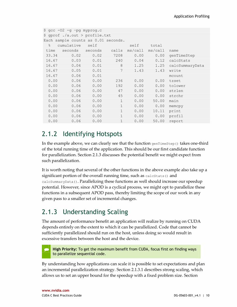
$ gcc -O2 -g –pg myprog.c
$ gprof ./a.out > profile.txt
Each sample counts as 0.01 seconds.
% cumulative self self total
time seconds seconds calls ms/call ms/call name
33.34 0.02 0.02 7208 0.00 0.00 genTimeStep
16.67 0.03 0.01 240 0.04 0.12 calcStats
16.67 0.04 0.01 8 1.25 1.25 calcSummaryData
16.67 0.05 0.01 7 1.43 1.43 write
16.67 0.06 0.01 mcount
0.00 0.06 0.00 236 0.00 0.00 tzset
0.00 0.06 0.00 192 0.00 0.00 tolower
0.00 0.06 0.00 47 0.00 0.00 strlen
0.00 0.06 0.00 45 0.00 0.00 strchr
0.00 0.06 0.00 1 0.00 50.00 main
0.00 0.06 0.00 1 0.00 0.00 memcpy
0.00 0.06 0.00 1 0.00 10.11 print
0.00 0.06 0.00 1 0.00 0.00 profil
0.00 0.06 0.00 1 0.00 50.00 report
2.1.2 Identifying Hotspots
In the example above, we can clearly see that the function genTimeStep() takes one-third
of the total running time of the application. This should be our first candidate function
for parallelization. Section 2.1.3 discusses the potential benefit we might expect from
such parallelization.
It is worth noting that several of the other functions in the above example also take up a
significant portion of the overall running time, such as calcStats() and
calcSummaryData(). Parallelizing these functions as well should increase our speedup
potential. However, since APOD is a cyclical process, we might opt to parallelize these
functions in a subsequent APOD pass, thereby limiting the scope of our work in any
given pass to a smaller set of incremental changes.
2.1.3 Understanding Scaling
The amount of performance benefit an application will realize by running on CUDA
depends entirely on the extent to which it can be parallelized. Code that cannot be
sufficiently parallelized should run on the host, unless doing so would result in
excessive transfers between the host and the device.
High Priority: To get the maximum benefit from CUDA, focus first on finding ways to parallelize sequential code.
By understanding how applications can scale it is possible to set expectations and plan
an incremental parallelization strategy. Section 2.1.3.1 describes strong scaling, which
allows us to set an upper bound for the speedup with a fixed problem size. Section

Application Profiling
www.nvidia.com
CUDA C Best Practices Guide DG-05603-001_v4.1 | 11
2.1.3.2 describes weak scaling, where the speedup is attained by growing the problem
size. In many applications, a combination of strong and weak scaling is desirable.
2.1.3.1 Strong scaling and Amdahl’s Law
Strong scaling is a measure of how, for a fixed overall problem size, the time to solution
decreases as more processors are added to a system. An application that exhibits linear
strong scaling has a speedup equal to the number of processors used.
Strong scaling is usually equated with Amdahl’s Law, which specifies the maximum
speedup that can be expected by parallelizing portions of a serial program. Essentially, it
states that the maximum speedup S of a program is:
Here P is the fraction of the total serial execution time taken by the portion of code that
can be parallelized and N is the number of processors over which the parallel portion of
the code runs.
The larger N is (that is, the greater the number of processors), the smaller the P/N
fraction. It can be simpler to view N as a very large number, which essentially
transforms the equation into S = 1 / (1 P). Now, if ¾ of the running time of a sequential
program is parallelized, the maximum speedup over serial code is 1 / (1 – ¾) = 4.
In reality, most applications do not exhibit perfectly linear strong scaling, even if they do
exhibit some degree of strong scaling. For most purposes, the key point is that the larger
the parallelizable portion P is, the greater the potential speedup. Conversely, if P is a
small number (meaning that the application is not substantially parallelizable),
increasing the number of processors N does little to improve performance. Therefore, to
get the largest speedup for a fixed problem size, it is worthwhile to spend effort on
increasing P, maximizing the amount of code that can be parallelized.
2.1.3.2 Weak scaling and Gustafson’s Law
Weak scaling is a measure of how the time to solution changes as more processors are
added to a system with a fixed problem size per processor; i.e., where the overall problem
size increases as the number of processors is increased.
Weak scaling is often equated with Gustafson’s Law, which states that in practice, the
problem size scales with the number of processors. Because of this, the maximum
speedup S of a program is:

Application Profiling
www.nvidia.com
CUDA C Best Practices Guide DG-05603-001_v4.1 | 12
Here P is the fraction of the total serial execution time taken by the portion of code that
can be parallelized and N is the number of processors over which the parallel portion of
the code runs.
Another way of looking at Gustafson’s Law is that it is not the problem size that remains
constant as we scale up the system but rather the execution time. Note that Gustafson’s
Law assumes that the ratio of serial to parallel execution remains constant, reflecting
additional cost in setting up and handling the larger problem.
2.1.3.3 Applying Strong and Weak Scaling
Understanding which type of scaling is most applicable to an application is an important
part of estimating speedup. For some applications the problem size will remain constant
and hence only strong scaling is applicable. An example would be modeling how two
molecules interact with each other, where the molecule sizes are fixed.
For other applications, the problem size will grow to fill the available processors.
Examples include modeling fluids or structures as meshes or grids and some Monte
Carlo simulations, where increasing the problem size provides increased accuracy.
Having understood the application profile, the developer should understand how the
problem size would change if the computational performance changes and then apply
either Amdahl’s or Gustafson’s Law to determine an upper bound for the speedup.
www.nvidia.com
CUDA C Best Practices Guide DG-05603-001_v4.1 | 13
PARALLELIZING YOUR APPLICATION
Having identified the hotspots and having done the basic exercises to set goals and
expectations, the developer needs to parallelize the code. Depending on the original
code, this can be as simple as calling into an existing GPU-optimized library such as
cuBLAS, cuFFT, or Thrust, or it could be as simple as adding a few preprocessor
directives as hints to a parallelizing compiler.
On the other hand, some applications’ designs will require some amount of refactoring
to expose their inherent parallelism. As even future CPU architectures will require
exposing this parallelism in order to improve or simply maintain the performance of
sequential applications, the CUDA family of parallel programming languages (CUDA
C/C++, CUDA Fortran, etc.) aims to make the expression of this parallelism as simple as
possible, while simultaneously enabling operation on CUDA-capable GPUs designed for
maximum parallel throughput.
www.nvidia.com
CUDA C Best Practices Guide DG-05603-001_v4.1 | 14
Chapter 3. GETTING STARTED
There are several key strategies for parallelizing sequential code. While the details of
how to apply these strategies to a particular application is a complex and problem-
specific topic, the general themes listed here apply regardless of whether we are
parallelizing code to run on for multicore CPUs or for use on CUDA GPUs.
3.1 PARALLEL LIBRARIES
The most straightforward approach to parallelizing an application is to leverage existing
libraries that take advantage of parallel architectures on our behalf. The CUDA Toolkit
includes a number of such libraries that have been fine-tuned for NVIDIA CUDA GPUs,
such as cuBLAS, cuFFT, and so on.
The key here is that libraries are most useful when they match well with the needs of the
application. Applications already using other BLAS libraries can often quite easily
switch to cuBLAS, for example, whereas applications that do little to no linear algebra
will have little use for cuBLAS. The same goes for other CUDA Toolkit libraries: cuFFT
has an interface similar to that of FFTW, etc.
Also of note is the Thrust library, which is a parallel C++ template library similar to the
C++ Standard Template Library. Thrust provides a rich collection of data parallel
primitives such as scan, sort, and reduce, which can be composed together to implement
complex algorithms with concise, readable source code. By describing your computation
in terms of these high-level abstractions you provide Thrust with the freedom to select
the most efficient implementation automatically. As a result, Thrust can be utilized in
rapid prototyping of CUDA applications, where programmer productivity matters most,
as well as in production, where robustness and absolute performance are crucial.

Getting Started
www.nvidia.com
CUDA C Best Practices Guide DG-05603-001_v4.1 | 15
3.2 PARALLELIZING COMPILERS
Another common approach to parallelization of sequential codes is to make use of
parallelizing compilers. Often this means the use of directives-based approaches, where
the programmer uses a pragma or other similar notation to provide hints to the compiler
about where parallelism can be found without needing to modify or adapt the
underlying code itself. By exposing parallelism to the compiler, directives allow the
compiler to do the detailed work of mapping the computation onto the parallel
architecture.
The OpenACC standard provides a set of compiler directives to specify loops and
regions of code in standard C, C++ and Fortran that should be offloaded from a host
CPU to an attached accelerator such as a CUDA GPU. The details of managing the
accelerator device are handled implicitly by an OpenACC-enabled compiler and
runtime.
See http://www.openacc-standard.org/ for details.
3.3 CODING TO EXPOSE PARALLELISM
For applications that need additional functionality or performance beyond what existing
parallel libraries or parallelizing compilers can provide, parallel programming
languages such as CUDA C/C++ that integrate seamlessly with existing sequential code
are essential.
Once we have located a hotspot in our application’s profile assessment and determined
that custom code is the best approach, we can use CUDA C/C++ to expose the
parallelism in that portion of our code as a CUDA kernel. We can then launch this kernel
onto the GPU and retrieve the results without requiring major rewrites to the rest of our
application.
This approach is most straightforward when the majority of the total running time of
our application is spent in a few relatively isolated portions of the code. More difficult to
parallelize are applications with a very flat profile – i.e., applications where the time
spent is spread out relatively evenly across a wide portion of the code base. For the latter
variety of application, some degree of code refactoring to expose the inherent
parallelism in the application might be necessary, but keep in mind that this refactoring
work will tend to benefit all future architectures, CPU and GPU alike, so it is well worth
the effort should it become necessary.
www.nvidia.com
CUDA C Best Practices Guide DG-05603-001_v4.1 | 16
Chapter 4. GETTING THE RIGHT ANSWER
Obtaining the right answer is clearly the principal goal of all computation. On parallel
systems, it is possible to run into difficulties not typically found in traditional serial-
oriented programming. These include threading issues, unexpected values due to the
way floating-point values are computed, and challenges arising from differences in the
way CPU and GPU processors operate. This chapter examines issues that can affect the
correctness of returned data and points to appropriate solutions.
4.1 VERIFICATION
4.1.1 Reference Comparison
A key aspect of correctness verification for modifications to any existing program is to
establish some mechanism whereby previous known-good reference outputs from
representative inputs can be compared to new results. After each change is made, ensure
that the results match using whatever criteria apply to the particular algorithm. Some
will expect bitwise identical results, which is not always possible, especially where
floating-point arithmetic is concerned; see Section 4.3 regarding numerical accuracy. For
other algorithms, implementations may be considered correct if they match the reference
within some small epsilon.
Note that the process used for validating numerical results can easily be extended to
validate performance results as well. We want to ensure that each change we make is
correct and that it improves performance (and by how much). Checking these things
frequently as an integral part of our cyclical APOD process will help ensure that we
achieve the desired results as rapidly as possible.
Getting The Right Answer
www.nvidia.com
CUDA C Best Practices Guide DG-05603-001_v4.1 | 17
4.1.2 Unit Testing
A useful counterpart to the reference comparisons described above is to structure the
code itself in such a way that is readily verifiable at the unit level. For example, we can
write our CUDA kernels as a collection of many short __device__ functions rather than
one large monolithic __global__ function; each device function can be tested
independently before hooking them all together.
For example, many kernels have complex addressing logic for accessing memory in
addition to their actual computation. If we validate our addressing logic separately prior
to introducing the bulk of the computation, then this will simplify any later debugging
efforts. (Note that the CUDA compiler considers any device code that does not
contribute to a write to global memory as dead code subject to elimination, so we must
at least write something out to global memory as a result of our addressing logic in order
to successfully apply this strategy.)
Going a step further, if most functions are defined as __host__ __device__ rather than
just __device__ functions, then these functions can be tested on both the CPU and the
GPU, thereby increasing our confidence that the function is correct and that there will
not be any unexpected differences in the results. If there are differences, then those
differences will be seen early and can be understood in the context of a simple function.
As a useful side effect, this strategy will allow us a means to reduce code duplication
should we wish to include both CPU and GPU execution paths in our application: if the
bulk of the work of our CUDA kernels is done in __host__ __device__ functions, we can
easily call those functions from both the host code and the device code without
duplication.
4.2 DEBUGGING
CUDA-GDB is a port of the GNU Debugger that runs on Linux and Mac; see
http://developer.nvidia.com/cuda-gdb.
The NVIDIA Parallel Nsight debugging and profiling tool for Microsoft Windows Vista
and Windows 7 is available as a free plugin for Microsoft Visual Studio; see
http://developer.nvidia.com/nvidia-parallel-nsight.
Several third-party debuggers now support CUDA debugging as well; see
http://developer.nvidia.com/debugging-solutions for more details.

Getting The Right Answer
www.nvidia.com
CUDA C Best Practices Guide DG-05603-001_v4.1 | 18
4.3 NUMERICAL ACCURACY AND PRECISION
Incorrect or unexpected results arise principally from issues of floating-point accuracy
due to the way floating-point values are computed and stored. The following sections
explain the principal items of interest. Other peculiarities of floating-point arithmetic are
presented in Section F.2 of the CUDA C Programming Guide as well as in a whitepaper
and accompanying webinar on floating-point precision and performance available from
http://developer.nvidia.com/content/precision-performance-floating-point-and-ieee-754-
compliance-nvidia-gpus.
4.3.1 Single vs. Double Precision
Devices of compute capability 1.3 and higher provide native support for double-
precision floating-point values (that is, values 64 bits wide). Results obtained using
double-precision arithmetic will frequently differ from the same operation performed
via single-precision arithmetic due to the greater precision of the former and due to
rounding issues. Therefore, it is important to be sure to compare like with like and to
express the results within a certain tolerance rather than expecting them to be exact.
Whenever doubles are used, use at least the –arch=sm_13 switch on the nvcc command
line; see Sections 3.1.3 and 3.1.4 of the CUDA C Programming Guide for more details.
4.3.2 Floating-Point Math Is Not Associative
Each floating-point arithmetic operation involves a certain amount of rounding.
Consequently, the order in which arithmetic operations are performed is important. If A,
B, and C are floating-point values, (A+B)+C is not guaranteed to equal A+(B+C) as it is in
symbolic math. When you parallelize computations, you potentially change the order of
operations and therefore the parallel results might not match sequential results. This
limitation is not specific to CUDA, but an inherent part of parallel computation on
floating-point values.
4.3.3 Promotions to Doubles and Truncations to Floats
When comparing the results of computations of float variables between the host and
device, make sure that promotions to double precision on the host do not account for
different numerical results. For example, if the code segment
float a;
…
a = a*1.02;
were performed on a device of compute capability 1.2 or less, or on a device with
compute capability 1.3 but compiled without enabling double precision (as mentioned
Getting The Right Answer
www.nvidia.com
CUDA C Best Practices Guide DG-05603-001_v4.1 | 19
above), then the multiplication would be performed in single precision. However, if the
code were performed on the host, the literal 1.02 would be interpreted as a double-
precision quantity and a would be promoted to a double, the multiplication would be
performed in double precision, and the result would be truncated to a float—thereby
yielding a slightly different result. If, however, the literal 1.02 were replaced with 1.02f,
the result would be the same in all cases because no promotion to doubles would occur.
To ensure that computations use single-precision arithmetic, always use float literals.
In addition to accuracy, the conversion between doubles and floats (and vice versa) has
a detrimental effect on performance, as discussed in Chapter 8.
4.3.4 IEEE 754 Compliance
All CUDA compute devices follow the IEEE 754 standard for binary floating-point
representation, with some small exceptions. These exceptions, which are detailed in
Section F.2 of the CUDA C Programming Guide, can lead to results that differ from IEEE
754 values computed on the host system.
One of the key differences is the fused multiply-add (FMA) instruction, which combines
multiply-add operations into a single instruction execution. Its result will often differ
slightly from results obtained by doing the two operations separately.
4.3.5 x86 80-bit Computations
x86 processors can use an 80-bit “double extended precision” math when performing
floating-point calculations. The results of these calculations can frequently differ from
pure 64-bit operations performed on the CUDA device. To get a closer match between
values, set the x86 host processor to use regular double or single precision (64 bits and
32 bits, respectively). This is done with the FLDCW assembly instruction or the equivalent
operating system API.
www.nvidia.com
CUDA C Best Practices Guide DG-05603-001_v4.1 | 20
OPTIMIZING CUDA APPLICATIONS
After each round of application parallelization is complete, the developer can move to
optimizing the implementation to improve performance. Since there are many possible
optimizations that can be considered, having a good understanding of the needs of the
application can help to make the process as smooth as possible. However, as with APOD
as a whole, program optimization is an iterative process (identify an opportunity for
optimization, apply and test the optimization, verify the speedup achieved, and repeat),
meaning that it is not necessary for a programmer to spend large amounts of time
memorizing the bulk of all possible optimization strategies prior to seeing good
speedups. Instead, strategies can be applied incrementally as they are learned.
Optimizations can be applied at various levels, from overlapping data transfers with
computation all the way down to fine-tuning floating-point operation sequences. The
available profiling tools are invaluable for guiding this process, as they can help suggest
a next-best course of action for the developer’s optimization efforts and provide
references into the relevant portions of the optimization section of this guide.
www.nvidia.com
CUDA C Best Practices Guide DG-05603-001_v4.1 | 21
Chapter 5. PERFORMANCE METRICS
When attempting to optimize CUDA code, it pays to know how to measure performance
accurately and to understand the role that bandwidth plays in performance
measurement. This chapter discusses how to correctly measure performance using CPU
timers and CUDA events. It then explores how bandwidth affects performance metrics
and how to mitigate some of the challenges it poses.
5.1 TIMING
CUDA calls and kernel executions can be timed using either CPU or GPU timers. This
section examines the functionality, advantages, and pitfalls of both approaches.
5.1.1 Using CPU Timers
Any CPU timer can be used to measure the elapsed time of a CUDA call or kernel
execution. The details of various CPU timing approaches are outside the scope of this
document, but developers should always be aware of the resolution their timing calls
provide.
When using CPU timers, it is critical to remember that many CUDA API functions are
asynchronous; that is, they return control back to the calling CPU thread prior to
completing their work. All kernel launches are asynchronous, as are memory-copy
functions with the Async suffix on their names. Therefore, to accurately measure the
elapsed time for a particular call or sequence of CUDA calls, it is necessary to
synchronize the CPU thread with the GPU by calling cudaDeviceSynchronize()
immediately before starting and stopping the CPU timer.

Performance Metrics
www.nvidia.com
CUDA C Best Practices Guide DG-05603-001_v4.1 | 22
cudaDeviceSynchronize()blocks the calling CPU thread until all CUDA calls previously
issued by the thread are completed.
Although it is also possible to synchronize the CPU thread with a particular stream or
event on the GPU, these synchronization functions are not suitable for timing code in
streams other than the default stream. cudaStreamSynchronize() blocks the CPU thread
until all CUDA calls previously issued into the given stream have completed.
cudaEventSynchronize() blocks until a given event in a particular stream has been
recorded by the GPU. Because the driver may interleave execution of CUDA calls from
other non-default streams, calls in other streams may be included in the timing.
Because the default stream, stream 0, exhibits serializing behavior for work on the
device (an operation in the default stream can begin only after all preceding calls in any
stream have completed; and no subsequent operation in any stream can begin until it
finishes), these functions can be used reliably for timing in the default stream.
Be aware that CPU-to-GPU synchronization points such as those mentioned in this
section imply a stall in the GPU’s processing pipeline and should thus be used sparingly
to minimize their performance impact.
5.1.2 Using CUDA GPU Timers
The CUDA event API provides calls that create and destroy events, record events (via
timestamp), and convert timestamp differences into a floating-point value in
milliseconds. Listing 5.1 illustrates their use.
cudaEvent_t start, stop;
float time;
cudaEventCreate(&start);
cudaEventCreate(&stop);
cudaEventRecord( start, 0 );
kernel<<<grid,threads>>> ( d_odata, d_idata, size_x, size_y,
NUM_REPS);
cudaEventRecord( stop, 0 );
cudaEventSynchronize( stop );
cudaEventElapsedTime( &time, start, stop );
cudaEventDestroy( start );
cudaEventDestroy( stop );
Listing 5.1 How to time code using CUDA events
Here cudaEventRecord() is used to place the start and stop events into the default
stream, stream 0. The device will record a timestamp for the event when it reaches that
event in the stream. The cudaEventElapsedTime() function returns the time elapsed
between the recording of the start and stop events. This value is expressed in
Performance Metrics
www.nvidia.com
CUDA C Best Practices Guide DG-05603-001_v4.1 | 23
milliseconds and has a resolution of approximately half a microsecond. Like the other
calls in this listing, their specific operation, parameters, and return values are described
in the CUDA Toolkit Reference Manual. Note that the timings are measured on the GPU
clock, so the timing resolution is operating-system-independent.
5.2 BANDWIDTH
Bandwidth—the rate at which data can be transferred—is one of the most important
gating factors for performance. Almost all changes to code should be made in the
context of how they affect bandwidth. As described in Chapter 6 of this guide,
bandwidth can be dramatically affected by the choice of memory in which data is stored,
how the data is laid out and the order in which it is accessed, as well as other factors.
To measure performance accurately, it is useful to calculate theoretical and effective
bandwidth. When the latter is much lower than the former, design or implementation
details are likely to reduce bandwidth, and it should be the primary goal of subsequent
optimization efforts to increase it.
High Priority: Use the effective bandwidth of your computation as a metric when measuring performance and optimization benefits.
5.2.1 Theoretical Bandwidth Calculation
Theoretical bandwidth can be calculated using hardware specifications available in the
product literature. For example, the NVIDIA Tesla M2090 uses GDDR5 (double data
rate) RAM with a memory clock rate of 1.85 GHz and a 384-bit-wide memory interface.
Using these data items, the peak theoretical memory bandwidth of the NVIDIA Tesla
M2090 is 177.6 GB/sec:
( 1.85 × 10⁹ × ( 384/8 ) × 2 ) / 109 = 177.6 GB/sec
In this calculation, the memory clock rate is converted in to Hz, multiplied by the
interface width (divided by 8, to convert bits to bytes) and multiplied by 2 due to the
double data rate. Finally, this product is divided by 109 to convert the result to GB/s.
Note that some calculations use 10243 instead of 109 for the final calculation. In such a
case, the bandwidth would be 165.4GB/s. It is important to use the same divisor when
calculating theoretical and effective bandwidth so that the comparison is valid.
5.2.2 Effective Bandwidth Calculation
Effective bandwidth is calculated by timing specific program activities and by knowing
how data is accessed by the program. To do so, use this equation:
Performance Metrics
www.nvidia.com
CUDA C Best Practices Guide DG-05603-001_v4.1 | 24
Effective bandwidth = (( Br + Bw ) / 109 ) / time
Here, the effective bandwidth is in units of GB/s, Br is the number of bytes read per
kernel, Bw is the number of bytes written per kernel, and time is given in seconds.
For example, to compute the effective bandwidth of a 2048 x 2048 matrix copy, the
following formula could be used:
Effective bandwidth = (( 20482 x 4 x 2 ) / 109 ) / time
The number of elements is multiplied by the size of each element (4 bytes for a float),
multiplied by 2 (because of the read and write), divided by 109 (or 1,0243) to obtain GB of
memory transferred. This number is divided by the time in seconds to obtain GB/s.
5.2.3 Throughput Reported by Visual Profiler
For devices with compute capability of 2.0 or greater, the Visual Profiler can be used to
collect several different memory throughput measures. The following throughput
metrics can be displayed in the Details or Detail Graphs view:
Requested Global Load Throughput
Requested Global Store Throughput
Global Load Throughput
Global Store Throughput
DRAM Read Throughput
DRAM Write Throughput
The Requested Global Load Throughput and Requested Global Store Throughput values
indicate the global memory throughput requested by the kernel and therefore
correspond to the effective bandwidth obtained by the calculation shown under Effective
Bandwidth Calculation.
Because the minimum memory transaction size is larger than most word sizes, the actual
memory throughput required for a kernel can include the transfer of data not used by
the kernel. For global memory accesses, this actual throughput is reported by the Global
Load Throughput and Global Store Throughput values.
It’s important to note that both numbers are useful. The actual memory throughput
shows how close the code is to the hardware limit, and a comparison of the effective or
requested bandwidth to the actual bandwidth presents a good estimate of how much
bandwidth is wasted by suboptimal coalescing of memory accesses (see Section 6.2.1).
For global memory accesses, this comparison of requested memory bandwidth to actual
memory bandwidth is reported by the Global Memory Load Efficiency and Global
Memory Store Efficiency metrics.
Note: the Visual Profiler uses 10243 when converting bytes/sec to GB/sec.

www.nvidia.com
CUDA C Best Practices Guide DG-05603-001_v4.1 | 25
Chapter 6. MEMORY OPTIMIZATIONS
Memory optimizations are the most important area for performance. The goal is to
maximize the use of the hardware by maximizing bandwidth. Bandwidth is best served
by using as much fast memory and as little slow-access memory as possible. This
chapter discusses the various kinds of memory on the host and device and how best to
set up data items to use the memory effectively.
6.1 DATA TRANSFER BETWEEN HOST AND DEVICE
The peak theoretical bandwidth between the device memory and the GPU is much
higher (177.6 GB/s on the NVIDIA Tesla M2090, for example) than the peak theoretical
bandwidth between host memory and device memory (8 GB/s on the PCIe ×16 Gen2).
Hence, for best overall application performance, it is important to minimize data
transfer between the host and the device, even if that means running kernels on the GPU
that do not demonstrate any speedup compared with running them on the host CPU.
High Priority: Minimize data transfer between the host and the device, even if it means running some kernels on the device that do not show performance gains when compared with running them on the host CPU.
Intermediate data structures should be created in device memory, operated on by the
device, and destroyed without ever being mapped by the host or copied to host
memory.
Also, because of the overhead associated with each transfer, batching many small
transfers into one larger transfer performs significantly better than making each transfer
separately.
Memory Optimizations
www.nvidia.com
CUDA C Best Practices Guide DG-05603-001_v4.1 | 26
Finally, higher bandwidth between the host and the device is achieved when using page-
locked (or pinned) memory, as discussed in the CUDA C Programming Guide and Section
6.1.1 of this document.
6.1.1 Pinned Memory
Page-locked or pinned memory transfers attain the highest bandwidth between the host
and the device. On PCIe ×16 Gen2 cards, for example, pinned memory can attain greater
than 5 GB/s transfer rates.
Pinned memory is allocated using the cudaHostAlloc() functions in the Runtime API.
The bandwidthTest.cu program in the NVIDIA GPU Computing SDK shows how to use
these functions as well as how to measure memory transfer performance.
Pinned memory should not be overused. Excessive use can reduce overall system
performance because pinned memory is a scarce resource. How much is too much is
difficult to tell in advance, so as with all optimizations, test the applications and the
systems they run on for optimal performance parameters.
6.1.2 Asynchronous Transfers and Overlapping Transfers with Computation
Data transfers between the host and the device using cudaMemcpy() are blocking
transfers; that is, control is returned to the host thread only after the data transfer is
complete. The cudaMemcpyAsync() function is a non-blocking variant of cudaMemcpy() in
which control is returned immediately to the host thread. In contrast with cudaMemcpy(),
the asynchronous transfer version requires pinned host memory (see Section 6.1.1), and it
contains an additional argument, a stream ID. A stream is simply a sequence of
operations that are performed in order on the device. Operations in different streams
can be interleaved and in some cases overlapped—a property that can be used to hide
data transfers between the host and the device.
Asynchronous transfers enable overlap of data transfers with computation in two
different ways. On all CUDA-enabled devices, it is possible to overlap host computation
with asynchronous data transfers and with device computations. For example, Listing
6.1 demonstrates how host computation in the routine cpuFunction() is performed
while data is transferred to the device and a kernel using the device is executed.
cudaMemcpyAsync(a_d, a_h, size, cudaMemcpyHostToDevice, 0);
kernel<<<grid, block>>>(a_d);
cpuFunction();
Listing 6.1 Overlapping computation and data transfers
The last argument to the cudaMemcpyAsync() function is the stream ID, which in this case
uses the default stream, stream 0. The kernel also uses the default stream, and it will not
Memory Optimizations
www.nvidia.com
CUDA C Best Practices Guide DG-05603-001_v4.1 | 27
begin execution until the memory copy completes; therefore, no explicit synchronization
is needed. Because the memory copy and the kernel both return control to the host
immediately, the host function cpuFunction() overlaps their execution.
In Listing 6.1, the memory copy and kernel execution occur sequentially. On devices that
are capable of concurrent copy and compute, it is possible to overlap kernel execution on
the device with data transfers between the host and the device. Whether a device has
this capability is indicated by the deviceOverlap field of the cudaDeviceProp structure (or
listed in the output of the deviceQuery SDK sample). On devices that have this
capability, the overlap once again requires pinned host memory, and, in addition, the
data transfer and kernel must use different, non-default streams (streams with non-zero
stream IDs). Non-default streams are required for this overlap because memory copy,
memory set functions, and kernel calls that use the default stream begin only after all
preceding calls on the device (in any stream) have completed, and no operation on the
device (in any stream) commences until they are finished.
Listing 6.2 illustrates the basic technique.
cudaStreamCreate(&stream1);
cudaStreamCreate(&stream2);
cudaMemcpyAsync(a_d, a_h, size, cudaMemcpyHostToDevice, stream1);
kernel<<<grid, block, 0, stream2>>>(otherData_d);
Listing 6.2 Concurrent copy and execute
In this code, two streams are created and used in the data transfer and kernel executions
as specified in the last arguments of the cudaMemcpyAsync call and the kernel’s execution
configuration.
Listing 6.2 demonstrates how to overlap kernel execution with asynchronous data
transfer. This technique could be used when the data dependency is such that the data
can be broken into chunks and transferred in multiple stages, launching multiple kernels
to operate on each chunk as it arrives. Listing 6.3 and Listing 6.4 demonstrate this. They
produce equivalent results. The first segment shows the reference sequential
implementation, which transfers and operates on an array of N floats (where N is
assumed to be evenly divisible by nThreads).
cudaMemcpy(a_d, a_h, N*sizeof(float), dir);
kernel<<<N/nThreads, nThreads>>>(a_d);
Listing 6.3 Sequential copy and execute
size=N*sizeof(float)/nStreams;
Memory Optimizations
www.nvidia.com
CUDA C Best Practices Guide DG-05603-001_v4.1 | 28
for (i=0; i<nStreams; i++) {
offset = i*N/nStreams;
cudaMemcpyAsync(a_d+offset, a_h+offset, size, dir, stream[i]);
kernel<<<N/(nThreads*nStreams), nThreads, 0,
stream[i]>>>(a_d+offset);
}
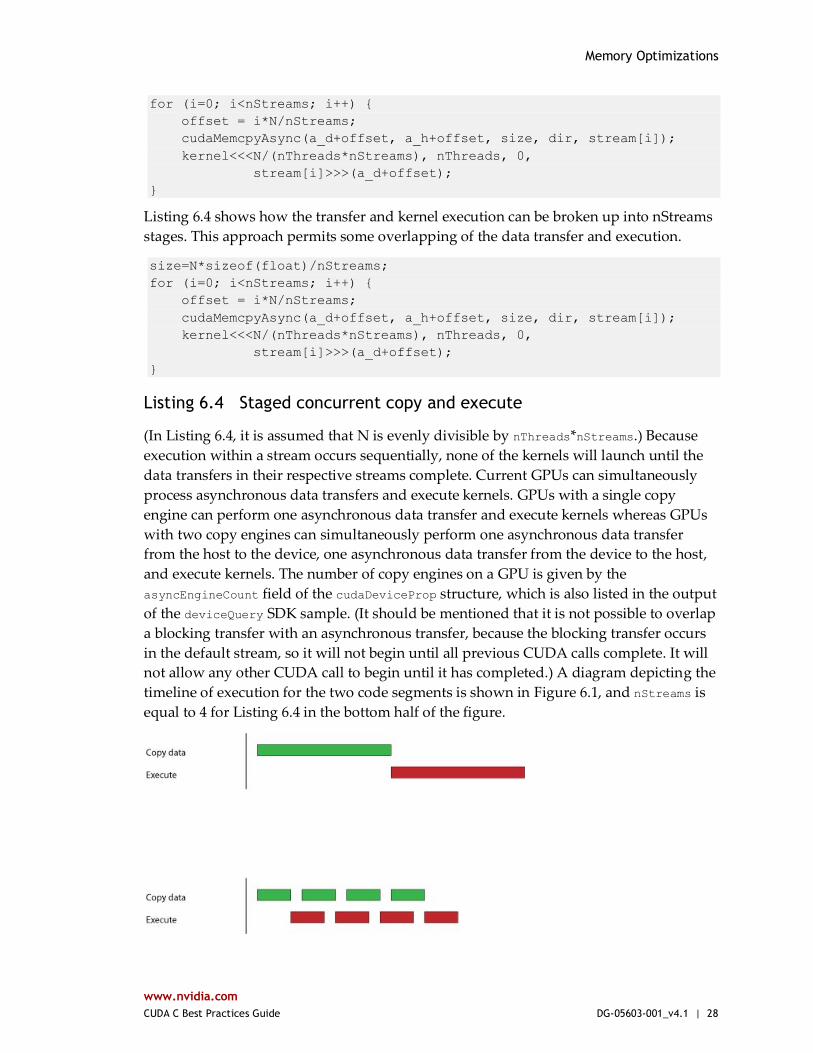
Listing 6.4 shows how the transfer and kernel execution can be broken up into nStreams
stages. This approach permits some overlapping of the data transfer and execution.
size=N*sizeof(float)/nStreams;
for (i=0; i<nStreams; i++) {
offset = i*N/nStreams;
cudaMemcpyAsync(a_d+offset, a_h+offset, size, dir, stream[i]);
kernel<<<N/(nThreads*nStreams), nThreads, 0,
stream[i]>>>(a_d+offset);
}
Listing 6.4 Staged concurrent copy and execute
(In Listing 6.4, it is assumed that N is evenly divisible by nThreads*nStreams.) Because
execution within a stream occurs sequentially, none of the kernels will launch until the
data transfers in their respective streams complete. Current GPUs can simultaneously
process asynchronous data transfers and execute kernels. GPUs with a single copy
engine can perform one asynchronous data transfer and execute kernels whereas GPUs
with two copy engines can simultaneously perform one asynchronous data transfer
from the host to the device, one asynchronous data transfer from the device to the host,
and execute kernels. The number of copy engines on a GPU is given by the
asyncEngineCount field of the cudaDeviceProp structure, which is also listed in the output
of the deviceQuery SDK sample. (It should be mentioned that it is not possible to overlap
a blocking transfer with an asynchronous transfer, because the blocking transfer occurs
in the default stream, so it will not begin until all previous CUDA calls complete. It will
not allow any other CUDA call to begin until it has completed.) A diagram depicting the
timeline of execution for the two code segments is shown in Figure 6.1, and nStreams is
equal to 4 for Listing 6.4 in the bottom half of the figure.
Memory Optimizations
www.nvidia.com
CUDA C Best Practices Guide DG-05603-001_v4.1 | 29
Figure 6.1 Timeline comparison for sequential (top) and concurrent (bottom) copy and kernel execution
For this example, it is assumed that the data transfer and kernel execution times are
comparable. In such cases, and when the execution time (tE) exceeds the transfer time
(tT), a rough estimate for the overall time is tE + tT/nStreams for the staged version versus
tE + tT for the sequential version. If the transfer time exceeds the execution time, a rough
estimate for the overall time is tT + tE/nStreams.
6.1.3 Zero Copy
Zero copy is a feature that was added in version 2.2 of the CUDA Toolkit. It enables GPU
threads to directly access host memory. For this purpose, it requires mapped pinned
(non-pageable) memory. On integrated GPUs (i.e., GPUs with the integrated field of the
CUDA device properties structure set to 1), mapped pinned memory is always a
performance gain because it avoids superfluous copies as integrated GPU and CPU
memory are physically the same. On discrete GPUs, mapped pinned memory is
advantageous only in certain cases. Because the data is not cached on the GPU, mapped
pinned memory should be read or written only once, and the global loads and stores
that read and write the memory should be coalesced. Zero copy can be used in place of
streams because kernel-originated data transfers automatically overlap kernel execution
without the overhead of setting up and determining the optimal number of streams.
Low Priority: Use zero-copy operations on integrated GPUs for CUDA Toolkit version 2.2 and later.
The host code in Listing 6.5 shows how zero copy is typically set up.
float *a_h, *a_map;
…
cudaGetDeviceProperties(&prop, 0);
if (!prop.canMapHostMemory)
exit(0);
cudaSetDeviceFlags(cudaDeviceMapHost);
cudaHostAlloc(&a_h, nBytes, cudaHostAllocMapped);
cudaHostGetDevicePointer(&a_map, a_h, 0);
kernel<<<gridSize, blockSize>>>(a_map);
Listing 6.5 Zero-copy host code
In this code, the canMapHostMemory field of the structure returned by
cudaGetDeviceProperties() is used to check that the device supports mapping host
memory to the device’s address space. Page-locked memory mapping is enabled by
calling cudaSetDeviceFlags() with cudaDeviceMapHost. Note that cudaSetDeviceFlags()
must be called prior to setting a device or making a CUDA call that requires state (that
is, essentially, before a context is created). Page-locked mapped host memory is

Memory Optimizations
www.nvidia.com
CUDA C Best Practices Guide DG-05603-001_v4.1 | 30
allocated using cudaHostAlloc(), and the pointer to the mapped device address space is
obtained via the function cudaHostGetDevicePointer(). In the code in Listing 6.5,
kernel() can reference the mapped pinned host memory using the pointer a_map in
exactly the same was as it would if a_map referred to a location in device memory.
Note: mapped pinned host memory allows you to overlap CPU-GPU memory transfers
with computation while avoiding the use of CUDA streams. But since any repeated
access to such memory areas causes repeated PCIe transfers, consider creating a second
area in device memory to manually cache the previously read host memory data.
6.1.4 Unified Virtual Addressing
Devices of compute capability 2.x support a special addressing mode called Unified
Virtual Addressing (UVA) on 64-bit Linux, MacOS, and Windows XP and on Windows
Vista/7 when using TCC driver mode. With UVA, the host memory and the device
memories of all installed supported devices share a single virtual address space.
Prior to UVA, an application had to keep track of which pointers referred to device
memory (and for which device) and which referred to host memory as a separate bit of
metadata (or as hard-coded information in the program) for each pointer. Using UVA,
on the other hand, the physical memory space to which a pointer points can be
determined simply by inspecting the value of the pointer using
cudaPointerGetAttributes().
Under UVA, pinned host memory allocated with cudaHostAlloc() will have identical
host and device pointers, so it is not necessary to call cudaHostGetDevicePointer() for
such allocations. Host memory allocations pinned after-the-fact via cudaHostRegister(),
however, will continue to have different device pointers than their host pointers, so
cudaHostGetDevicePointer() remains necessary in that case.
UVA is also a necessary precondition for enabling peer-to-peer (P2P) transfer of data
directly across the PCIe bus for supported GPUs in supported configurations, bypassing
host memory.
See the CUDA C Programming Guide for further explanations and software requirements
for UVA and P2P.
6.2 DEVICE MEMORY SPACES
CUDA devices use several memory spaces, which have different characteristics that
reflect their distinct usages in CUDA applications. These memory spaces include global,
local, shared, texture, and registers, as shown in Figure 6.2.
Memory Optimizations
www.nvidia.com
CUDA C Best Practices Guide DG-05603-001_v4.1 | 31
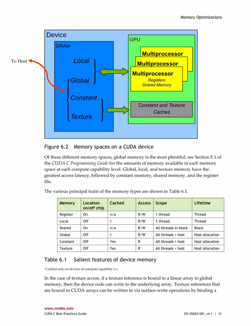
Figure 6.2 Memory spaces on a CUDA device
Of these different memory spaces, global memory is the most plentiful; see Section F.1 of
the CUDA C Programming Guide for the amounts of memory available in each memory
space at each compute capability level. Global, local, and texture memory have the
greatest access latency, followed by constant memory, shared memory, and the register
file.
The various principal traits of the memory types are shown in Table 6.1.
Memory Location
on/off chip
Cached Access Scope Lifetime
Register On n/a R/W 1 thread Thread
Local Off † R/W 1 thread Thread
Shared On n/a R/W All threads in block Block
Global Off † R/W All threads + host Host allocation
Constant Off Yes R All threads + host Host allocation
Texture Off Yes R All threads + host Host allocation
Table 6.1 Salient features of device memory
† Cached only on devices of compute capability 2.x.
In the case of texture access, if a texture reference is bound to a linear array in global
memory, then the device code can write to the underlying array. Texture references that
are bound to CUDA arrays can be written to via surface-write operations by binding a
Device
DRAM
Global
Constant
Texture
Local
GPU
Multiprocessor
Registers
Shared Memory Multiprocessor
Registers
Shared Memory Multiprocessor
Registers Shared Memory
Constant and Texture
Caches
To Host

Memory Optimizations
www.nvidia.com
CUDA C Best Practices Guide DG-05603-001_v4.1 | 32
surface to the same underlying CUDA array storage). Reading from a texture while
writing to its underlying global memory array in the same kernel launch should be
avoided because the texture caches are read-only and are not invalidated when the
associated global memory is modified.
6.2.1 Coalesced Access to Global Memory
Perhaps the single most important performance consideration in programming for the
CUDA architecture is the coalescing of global memory accesses. Global memory loads
and stores by threads of a warp (of a half warp for devices of compute capability 1.x) are
coalesced by the device into as few as one transaction when certain access requirements
are met.
High Priority: Ensure global memory accesses are coalesced whenever possible.
The access requirements for coalescing depend on the compute capability of the device
and are documented in the CUDA C Programming Guide (Section F.3.2 for compute
capability 1.x and Section F.4.2 for compute capability 2.x).
For devices of compute capability 2.x, the requirements can be summarized quite easily:
the concurrent accesses of the threads of a warp will coalesce into a number of
transactions equal to the number of cache lines necessary to service all of the threads of
the warp. By default, all accesses are cached through L1, which as 128-byte lines. For
scattered access patterns, to reduce overfetch, it can sometimes be useful to cache only in
L2, which caches shorter 32-byte segments (see the CUDA C Programming Guide).
Coalescing concepts are illustrated in the following simple examples. These examples
assume compute capability 2.x. These examples assume that accesses are cached through
L1, which is the default behavior, and that accesses are for 4-byte words, unless
otherwise noted.
For corresponding examples for compute capability 1.x, refer to earlier versions of this
guide.
6.2.1.1 A Simple Access Pattern
The first and simplest case of coalescing can be achieved by any CUDA-enabled device:
the k-th thread accesses the k-th word in a cache line. Not all threads need to participate.
For example, if the threads of a warp access adjacent 4-byte words (e.g., adjacent float
values), a single 128B L1 cache line and therefore a single coalesced transaction will
service that memory access. Such a pattern is shown in Figure 6.3.
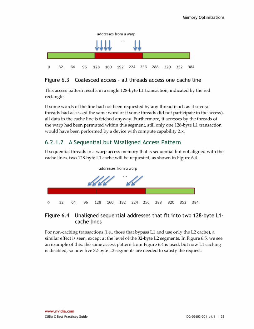
Memory Optimizations
www.nvidia.com
CUDA C Best Practices Guide DG-05603-001_v4.1 | 33
Figure 6.3 Coalesced access – all threads access one cache line
This access pattern results in a single 128-byte L1 transaction, indicated by the red
rectangle.
If some words of the line had not been requested by any thread (such as if several
threads had accessed the same word or if some threads did not participate in the access),
all data in the cache line is fetched anyway. Furthermore, if accesses by the threads of
the warp had been permuted within this segment, still only one 128-byte L1 transaction
would have been performed by a device with compute capability 2.x.
6.2.1.2 A Sequential but Misaligned Access Pattern
If sequential threads in a warp access memory that is sequential but not aligned with the
cache lines, two 128-byte L1 cache will be requested, as shown in Figure 6.4.
Figure 6.4 Unaligned sequential addresses that fit into two 128-byte L1-cache lines
For non-caching transactions (i.e., those that bypass L1 and use only the L2 cache), a
similar effect is seen, except at the level of the 32-byte L2 segments. In Figure 6.5, we see
an example of this: the same access pattern from Figure 6.4 is used, but now L1 caching
is disabled, so now five 32-byte L2 segments are needed to satisfy the request.
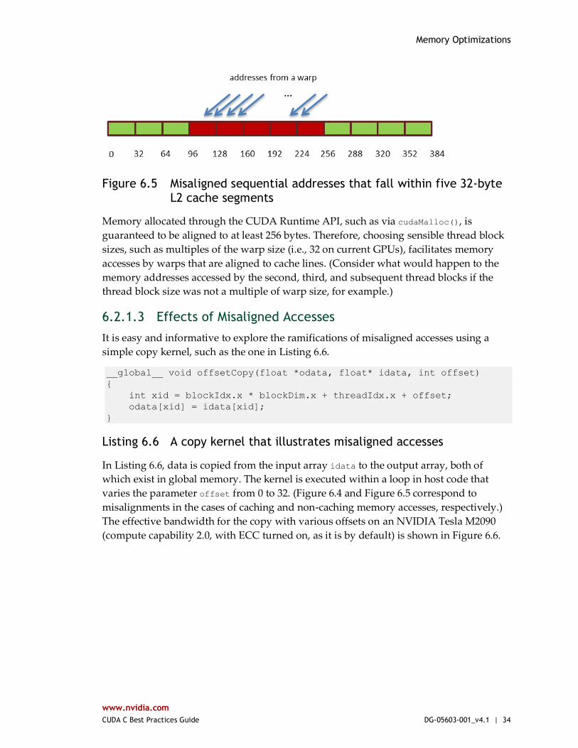
Memory Optimizations
www.nvidia.com
CUDA C Best Practices Guide DG-05603-001_v4.1 | 34
Figure 6.5 Misaligned sequential addresses that fall within five 32-byte L2 cache segments
Memory allocated through the CUDA Runtime API, such as via cudaMalloc(), is
guaranteed to be aligned to at least 256 bytes. Therefore, choosing sensible thread block
sizes, such as multiples of the warp size (i.e., 32 on current GPUs), facilitates memory
accesses by warps that are aligned to cache lines. (Consider what would happen to the
memory addresses accessed by the second, third, and subsequent thread blocks if the
thread block size was not a multiple of warp size, for example.)
6.2.1.3 Effects of Misaligned Accesses
It is easy and informative to explore the ramifications of misaligned accesses using a
simple copy kernel, such as the one in Listing 6.6.
__global__ void offsetCopy(float *odata, float* idata, int offset)
{
int xid = blockIdx.x * blockDim.x + threadIdx.x + offset;
odata[xid] = idata[xid];
}
Listing 6.6 A copy kernel that illustrates misaligned accesses
In Listing 6.6, data is copied from the input array idata to the output array, both of
which exist in global memory. The kernel is executed within a loop in host code that
varies the parameter offset from 0 to 32. (Figure 6.4 and Figure 6.5 correspond to
misalignments in the cases of caching and non-caching memory accesses, respectively.)
The effective bandwidth for the copy with various offsets on an NVIDIA Tesla M2090
(compute capability 2.0, with ECC turned on, as it is by default) is shown in Figure 6.6.

Memory Optimizations
www.nvidia.com
CUDA C Best Practices Guide DG-05603-001_v4.1 | 35
Figure 6.6 Performance of offsetCopy kernel
For the NVIDIA Tesla M2090, global memory accesses with no offset or with offsets that
are multiples of 32 words result in a single L1 cache line transaction or 4 L2 cache
segment loads (for non-L1-caching loads). The achieved bandwidth is approximately
130GB/s. Otherwise, either two L1 cache lines (caching mode) or four to five L2 cache
segments (non-caching mode) are loaded per warp, resulting in approximately 4/5th of
the memory throughput achieved with no offsets.
An interesting point is that we might expect the caching case to perform worse than the
non-caching case for this sample, given that each warp in the caching case fetches twice
as many bytes as it requires, whereas in the non-caching case, only 5/4 as many bytes as
required are fetched per warp. In this particular example, that effect is not apparent,
however, because adjacent warps reuse the cache lines their neighbors fetched. So while
the impact is still evident in the case of caching loads, it is not as great as we might have
expected. It would have been more so if adjacent warps had not exhibited such a high
degree of reuse of the over-fetched cache lines.
6.2.1.4 Strided Accesses
As seen above, in the case of misaligned sequential accesses, the caches of compute
capability 2.x devices help a lot to achieve reasonable performance. It may be different
with non-unit-strided accesses, however, and this is a pattern that occurs frequently
when dealing with multidimensional data or matrices. For this reason, ensuring that as
much as possible of the data in each cache line fetched is actually used is an important
part of performance optimization of memory accesses on these devices.
0
20
40
60
80
100
120
140
0 4 8 12 16 20 24 28 32
Ban
dw
idth
(G
B/s
)
Offset
Copy with Offset (Tesla M2090 - ECC on)
Caching
Non-caching
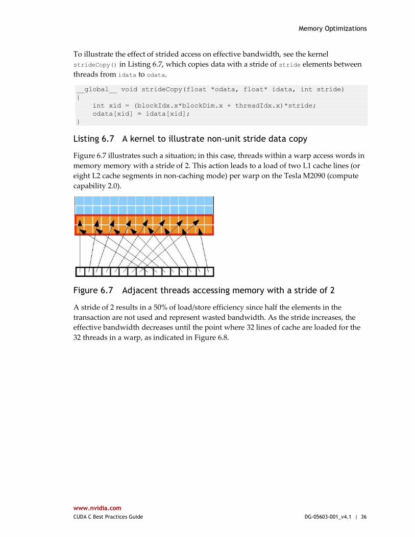
Memory Optimizations
www.nvidia.com
CUDA C Best Practices Guide DG-05603-001_v4.1 | 36
To illustrate the effect of strided access on effective bandwidth, see the kernel
strideCopy() in Listing 6.7, which copies data with a stride of stride elements between
threads from idata to odata.
__global__ void strideCopy(float *odata, float* idata, int stride)
{
int xid = (blockIdx.x*blockDim.x + threadIdx.x)*stride;
odata[xid] = idata[xid];
}
Listing 6.7 A kernel to illustrate non-unit stride data copy
Figure 6.7 illustrates such a situation; in this case, threads within a warp access words in
memory memory with a stride of 2. This action leads to a load of two L1 cache lines (or
eight L2 cache segments in non-caching mode) per warp on the Tesla M2090 (compute
capability 2.0).
Figure 6.7 Adjacent threads accessing memory with a stride of 2
A stride of 2 results in a 50% of load/store efficiency since half the elements in the
transaction are not used and represent wasted bandwidth. As the stride increases, the
effective bandwidth decreases until the point where 32 lines of cache are loaded for the
32 threads in a warp, as indicated in Figure 6.8.
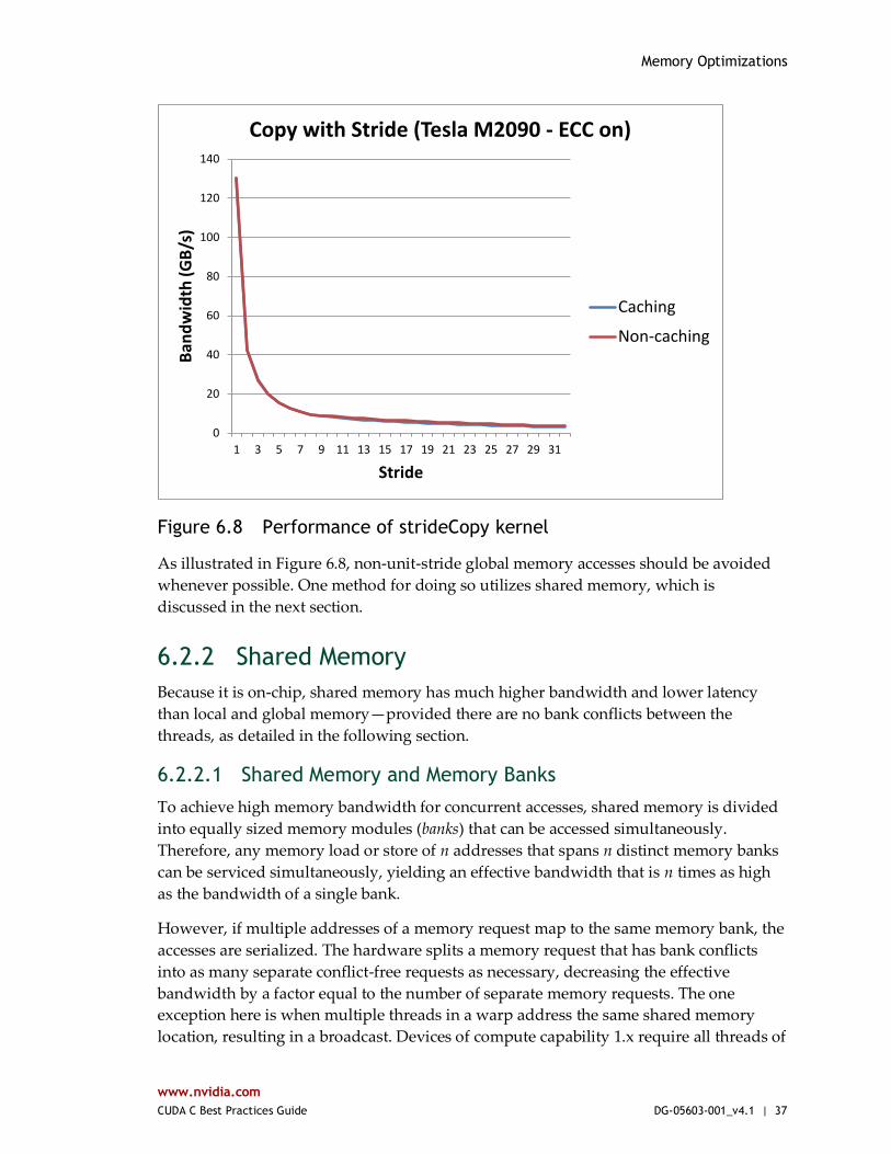
Memory Optimizations
www.nvidia.com
CUDA C Best Practices Guide DG-05603-001_v4.1 | 37
Figure 6.8 Performance of strideCopy kernel
As illustrated in Figure 6.8, non-unit-stride global memory accesses should be avoided
whenever possible. One method for doing so utilizes shared memory, which is
discussed in the next section.
6.2.2 Shared Memory
Because it is on-chip, shared memory has much higher bandwidth and lower latency
than local and global memory—provided there are no bank conflicts between the
threads, as detailed in the following section.
6.2.2.1 Shared Memory and Memory Banks
To achieve high memory bandwidth for concurrent accesses, shared memory is divided
into equally sized memory modules (banks) that can be accessed simultaneously.
Therefore, any memory load or store of n addresses that spans n distinct memory banks
can be serviced simultaneously, yielding an effective bandwidth that is n times as high
as the bandwidth of a single bank.
However, if multiple addresses of a memory request map to the same memory bank, the
accesses are serialized. The hardware splits a memory request that has bank conflicts
into as many separate conflict-free requests as necessary, decreasing the effective
bandwidth by a factor equal to the number of separate memory requests. The one
exception here is when multiple threads in a warp address the same shared memory
location, resulting in a broadcast. Devices of compute capability 1.x require all threads of
0
20
40
60
80
100
120
140
1 3 5 7 9 11 13 15 17 19 21 23 25 27 29 31
Ban
dw
idth
(G
B/s
)
Stride
Copy with Stride (Tesla M2090 - ECC on)
Caching
Non-caching
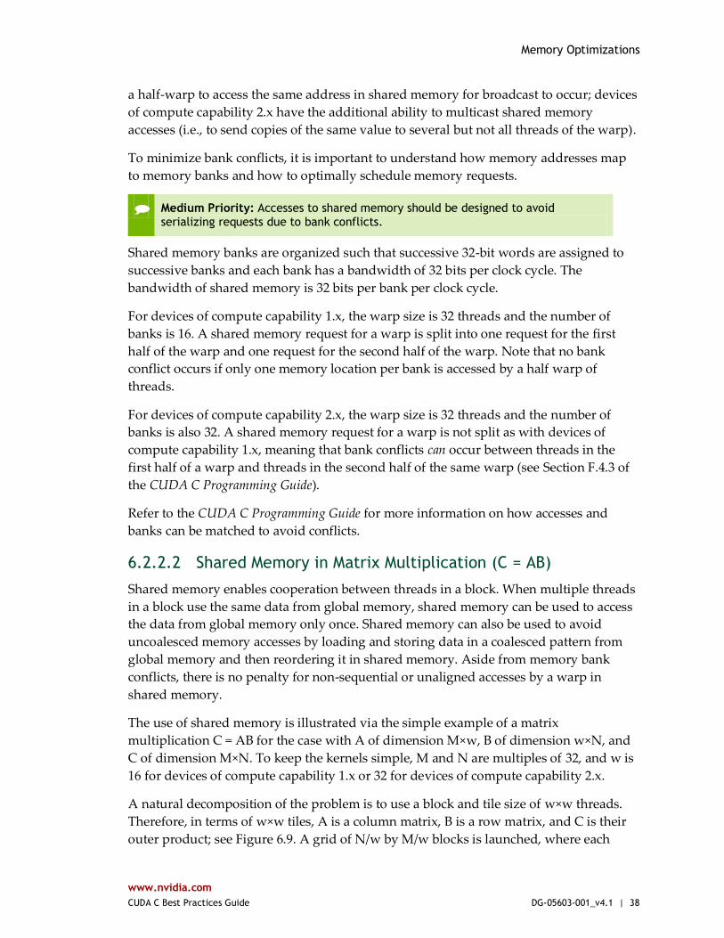
Memory Optimizations
www.nvidia.com
CUDA C Best Practices Guide DG-05603-001_v4.1 | 38
a half-warp to access the same address in shared memory for broadcast to occur; devices
of compute capability 2.x have the additional ability to multicast shared memory
accesses (i.e., to send copies of the same value to several but not all threads of the warp).
To minimize bank conflicts, it is important to understand how memory addresses map
to memory banks and how to optimally schedule memory requests.
Medium Priority: Accesses to shared memory should be designed to avoid serializing requests due to bank conflicts.
Shared memory banks are organized such that successive 32-bit words are assigned to
successive banks and each bank has a bandwidth of 32 bits per clock cycle. The
bandwidth of shared memory is 32 bits per bank per clock cycle.
For devices of compute capability 1.x, the warp size is 32 threads and the number of
banks is 16. A shared memory request for a warp is split into one request for the first
half of the warp and one request for the second half of the warp. Note that no bank
conflict occurs if only one memory location per bank is accessed by a half warp of
threads.
For devices of compute capability 2.x, the warp size is 32 threads and the number of
banks is also 32. A shared memory request for a warp is not split as with devices of
compute capability 1.x, meaning that bank conflicts can occur between threads in the
first half of a warp and threads in the second half of the same warp (see Section F.4.3 of
the CUDA C Programming Guide).
Refer to the CUDA C Programming Guide for more information on how accesses and
banks can be matched to avoid conflicts.
6.2.2.2 Shared Memory in Matrix Multiplication (C = AB)
Shared memory enables cooperation between threads in a block. When multiple threads
in a block use the same data from global memory, shared memory can be used to access
the data from global memory only once. Shared memory can also be used to avoid
uncoalesced memory accesses by loading and storing data in a coalesced pattern from
global memory and then reordering it in shared memory. Aside from memory bank
conflicts, there is no penalty for non-sequential or unaligned accesses by a warp in
shared memory.
The use of shared memory is illustrated via the simple example of a matrix
multiplication C = AB for the case with A of dimension M×w, B of dimension w×N, and
C of dimension M×N. To keep the kernels simple, M and N are multiples of 32, and w is
16 for devices of compute capability 1.x or 32 for devices of compute capability 2.x.
A natural decomposition of the problem is to use a block and tile size of w×w threads.
Therefore, in terms of w×w tiles, A is a column matrix, B is a row matrix, and C is their
outer product; see Figure 6.9. A grid of N/w by M/w blocks is launched, where each

Memory Optimizations
www.nvidia.com
CUDA C Best Practices Guide DG-05603-001_v4.1 | 39
thread block calculates the elements of a different tile in C from a single tile of A and a
single tile of B.
Figure 6.9 Block-column matrix (A) multiplied by block-row matrix (B) with resulting product matrix (C)
To do this, the simpleMultiply kernel (Listing 6.8) calculates the output elements of a tile
of matrix C.
__global__ void simpleMultiply(float *a, float* b, float *c,
int N)
{
int row = blockIdx.y * blockDim.y + threadIdx.y;
int col = blockIdx.x * blockDim.x + threadIdx.x;
float sum = 0.0f;
for (int i = 0; i < TILE_DIM; i++) {
sum += a[row*TILE_DIM+i] * b[i*N+col];
}
c[row*N+col] = sum;
}
Listing 6.8 Unoptimized matrix multiplication
In Listing 6.8, a, b, and c are pointers to global memory for the matrices A, B, and C,
respectively; blockDim.x, blockDim.y, and TILE_DIM are all equal to w. Each thread in the
w×w-thread block calculates one element in a tile of C. row and col are the row and
column of the element in C being calculated by a particular thread. The for loop over i
multiplies a row of A by a column of B, which is then written to C.
The effective bandwidth of this kernel is only 14.5GB/s on an NVIDIA Tesla M2090 (with
ECC on). To analyze performance, it is necessary to consider how warps access global

Memory Optimizations
www.nvidia.com
CUDA C Best Practices Guide DG-05603-001_v4.1 | 40
memory in the for loop. Each warp of threads calculates one row of a tile of C, which
depends on a single row of A and an entire tile of B as illustrated in Figure 6.10.
Figure 6.10 Computing a row of a tile in C using one row of A and an entire tile of B
For each iteration i of the for loop, the threads in a warp read a row of the B tile, which
is a sequential and coalesced access for all compute capabilities.
However, for each iteration i, all threads in a warp read the same value from global
memory for matrix A, as the index row*TILE_DIM+i is constant within a warp. Even
though such an access requires only 1 transaction on devices of compute capability 2.x,
there is wasted bandwidth in the transaction, because only one 4-byte word out of 32
words in the cache line is used. We can reuse this cache line in subsequent iterations of
the loop, and we would eventually utilize all 32 words; however, when many warps
execute on the same multiprocessor simultaneously, as is generally the case, the cache
line may easily be evicted from the cache between iterations i and i+1.
The performance on a device of any compute capability can be improved by reading a
tile of A into shared memory as shown in Listing 6.9.
__global__ void coalescedMultiply(float *a, float* b, float *c,
int N)
{
__shared__ float aTile[TILE_DIM][TILE_DIM];
int row = blockIdx.y * blockDim.y + threadIdx.y;
int col = blockIdx.x * blockDim.x + threadIdx.x;
float sum = 0.0f;
aTile[threadIdx.y][threadIdx.x] = a[row*TILE_DIM+threadIdx.x];
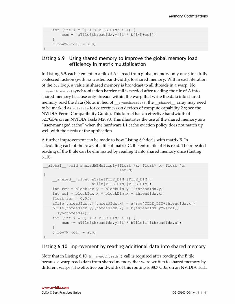
Memory Optimizations
www.nvidia.com
CUDA C Best Practices Guide DG-05603-001_v4.1 | 41
for (int i = 0; i < TILE_DIM; i++) {
sum += aTile[threadIdx.y][i]* b[i*N+col];
}
c[row*N+col] = sum;
}
Listing 6.9 Using shared memory to improve the global memory load efficiency in matrix multiplication
In Listing 6.9, each element in a tile of A is read from global memory only once, in a fully
coalesced fashion (with no wasted bandwidth), to shared memory. Within each iteration
of the for loop, a value in shared memory is broadcast to all threads in a warp. No
__syncthreads()synchronization barrier call is needed after reading the tile of A into
shared memory because only threads within the warp that write the data into shared
memory read the data (Note: in lieu of __syncthreads(), the __shared__ array may need
to be marked as volatile for correctness on devices of compute capability 2.x; see the
NVIDIA Fermi Compatibility Guide). This kernel has an effective bandwidth of
32.7GB/s on an NVIDIA Tesla M2090. This illustrates the use of the shared memory as a
“user-managed cache” when the hardware L1 cache eviction policy does not match up
well with the needs of the application.
A further improvement can be made to how Listing 6.9 deals with matrix B. In
calculating each of the rows of a tile of matrix C, the entire tile of B is read. The repeated
reading of the B tile can be eliminated by reading it into shared memory once (Listing
6.10).
__global__ void sharedABMultiply(float *a, float* b, float *c,
int N)
{
__shared__ float aTile[TILE_DIM][TILE_DIM],
bTile[TILE_DIM][TILE_DIM];
int row = blockIdx.y * blockDim.y + threadIdx.y;
int col = blockIdx.x * blockDim.x + threadIdx.x;
float sum = 0.0f;
aTile[threadIdx.y][threadIdx.x] = a[row*TILE_DIM+threadIdx.x];
bTile[threadIdx.y][threadIdx.x] = b[threadIdx.y*N+col];
__syncthreads();
for (int i = 0; i < TILE_DIM; i++) {
sum += aTile[threadIdx.y][i]* bTile[i][threadIdx.x];
}
c[row*N+col] = sum;
}
Listing 6.10 Improvement by reading additional data into shared memory
Note that in Listing 6.10, a __syncthreads() call is required after reading the B tile
because a warp reads data from shared memory that were written to shared memory by
different warps. The effective bandwidth of this routine is 38.7 GB/s on an NVIDIA Tesla

Memory Optimizations
www.nvidia.com
CUDA C Best Practices Guide DG-05603-001_v4.1 | 42
M2090. Note that the performance improvement is not due to improved coalescing in
either case, but to avoiding redundant transfers from global memory.
The results of the various optimizations are summarized in Table 6.2.
Optimization NVIDIA Tesla M2090
No optimization 14.5 GB/s
Coalesced using shared
memory to store a tile of A 32.7 GB/s
Using shared memory to
eliminate redundant reads
of a tile of B
38.7 GB/s
Table 6.2 Performance Improvements Optimizing C = AB Matrix Multiply
Medium Priority: Use shared memory to avoid redundant transfers from global memory.
6.2.2.3 Shared Memory in Matrix Multiplication (C = AAT)
A variant of the previous matrix multiplication can be used to illustrate how strided
accesses to global memory, as well as shared memory bank conflicts, are handled. This
variant simply uses the transpose of A in place of B, so C = AAT.
A simple implementation for C = AAT is shown in Listing 6.11.
__global__ void simpleMultiply(float *a, float *c, int M)
{
int row = blockIdx.y * blockDim.y + threadIdx.y;
int col = blockIdx.x * blockDim.x + threadIdx.x;
float sum = 0.0f;
for (int i = 0; i < TILE_DIM; i++) {
sum += a[row*TILE_DIM+i] * a[col*TILE_DIM+i];
}
c[row*M+col] = sum;
}
Listing 6.11 Unoptimized handling of strided accesses to global memory
In Listing 6.11, the row-th, col-th element of C is obtained by taking the dot product of
the row-th and col-th rows of A. The effective bandwidth for this kernel is 3.64 GB/s on
an NVIDIA Tesla M2090. These results are substantially lower than the corresponding
measurements for the C = AB kernel. The difference is in how threads in a half warp
access elements of A in the second term, a[col*TILE_DIM+i], for each iteration i. For a
warp of threads, col represents sequential columns of the transpose of A, and therefore

Memory Optimizations
www.nvidia.com
CUDA C Best Practices Guide DG-05603-001_v4.1 | 43
col*TILE_DIM represents a strided access of global memory with a stride of w, resulting
in plenty of wasted bandwidth.
The way to avoid strided access is to use shared memory as before, except in this case a
warp reads a row of A into a column of a shared memory tile, as shown in Listing 6.12.
__global__ void coalescedMultiply(float *a, float *c, int M)
{
__shared__ float aTile[TILE_DIM][TILE_DIM],
transposedTile[TILE_DIM][TILE_DIM];
int row = blockIdx.y * blockDim.y + threadIdx.y;
int col = blockIdx.x * blockDim.x + threadIdx.x;
float sum = 0.0f;
aTile[threadIdx.y][threadIdx.x] = a[row*TILE_DIM+threadIdx.x];
transposedTile[threadIdx.x][threadIdx.y] =
a[(blockIdx.x*blockDim.x + threadIdx.y)*TILE_DIM +
threadIdx.x];
__syncthreads();
for (int i = 0; i < TILE_DIM; i++) {
sum += aTile[threadIdx.y][i]* transposedTile[i][threadIdx.x];
}
c[row*M+col] = sum;
}
Listing 6.12 An optimized version of Listing 6.11 using coalesced reads from global memory
Listing 6.12 uses the shared transposedTile to avoid uncoalesced accesses in the second
term in the dot product and the shared aTile technique from the previous example to
avoid uncoalesced accesses in the first term. The effective bandwidth of this kernel is
27.5 GB/s on an NVIDIA Tesla M2090.These results are slightly lower than those
obtained by the final kernel for C = AB. The cause of the difference is shared memory
bank conflicts.
The reads of elements in transposedTile within the for loop are free of conflicts, because
threads of each half warp read across rows of the tile, resulting in unit stride across the
banks. However, bank conflicts occur when copying the tile from global memory into
shared memory. To enable the loads from global memory to be coalesced, data are read
from global memory sequentially. However, this requires writing to shared memory in
columns, and because of the use of w×w tiles in shared memory, this results in a stride
between threads of w banks – every thread of the warp hits the same bank. (Recall that
w is selected as 16 for devices of compute capability 1.x and 32 for devices of compute
capability 2.x.) These many-way bank conflicts are very expensive. The simple remedy is
to pad the shared memory array so that it has an extra column, as in the following line of
code.
__shared__ float transposedTile[TILE_DIM][TILE_DIM+1];
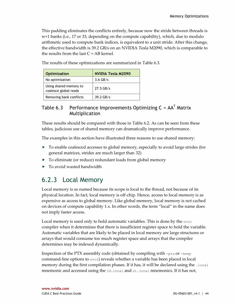
Memory Optimizations
www.nvidia.com
CUDA C Best Practices Guide DG-05603-001_v4.1 | 44
This padding eliminates the conflicts entirely, because now the stride between threads is
w+1 banks (i.e., 17 or 33, depending on the compute capability), which, due to modulo
arithmetic used to compute bank indices, is equivalent to a unit stride. After this change,
the effective bandwidth is 39.2 GB/s on an NVIDIA Tesla M2090, which is comparable to
the results from the last C = AB kernel.
The results of these optimizations are summarized in Table 6.3.
Optimization NVIDIA Tesla M2090
No optimization 3.6 GB/s
Using shared memory to
coalesce global reads 27.5 GB/s
Removing bank conflicts 39.2 GB/s
Table 6.3 Performance Improvements Optimizing C = AAT Matrix Multiplication
These results should be compared with those in Table 6.2. As can be seen from these
tables, judicious use of shared memory can dramatically improve performance.
The examples in this section have illustrated three reasons to use shared memory:
To enable coalesced accesses to global memory, especially to avoid large strides (for
general matrices, strides are much larger than 32)
To eliminate (or reduce) redundant loads from global memory
To avoid wasted bandwidth
6.2.3 Local Memory
Local memory is so named because its scope is local to the thread, not because of its
physical location. In fact, local memory is off-chip. Hence, access to local memory is as
expensive as access to global memory. Like global memory, local memory is not cached
on devices of compute capability 1.x. In other words, the term “local” in the name does
not imply faster access.
Local memory is used only to hold automatic variables. This is done by the nvcc
compiler when it determines that there is insufficient register space to hold the variable.
Automatic variables that are likely to be placed in local memory are large structures or
arrays that would consume too much register space and arrays that the compiler
determines may be indexed dynamically.
Inspection of the PTX assembly code (obtained by compiling with -ptx or -keep
command-line options to nvcc) reveals whether a variable has been placed in local
memory during the first compilation phases. If it has, it will be declared using the .local
mnemonic and accessed using the ld.local and st.local mnemonics. If it has not,
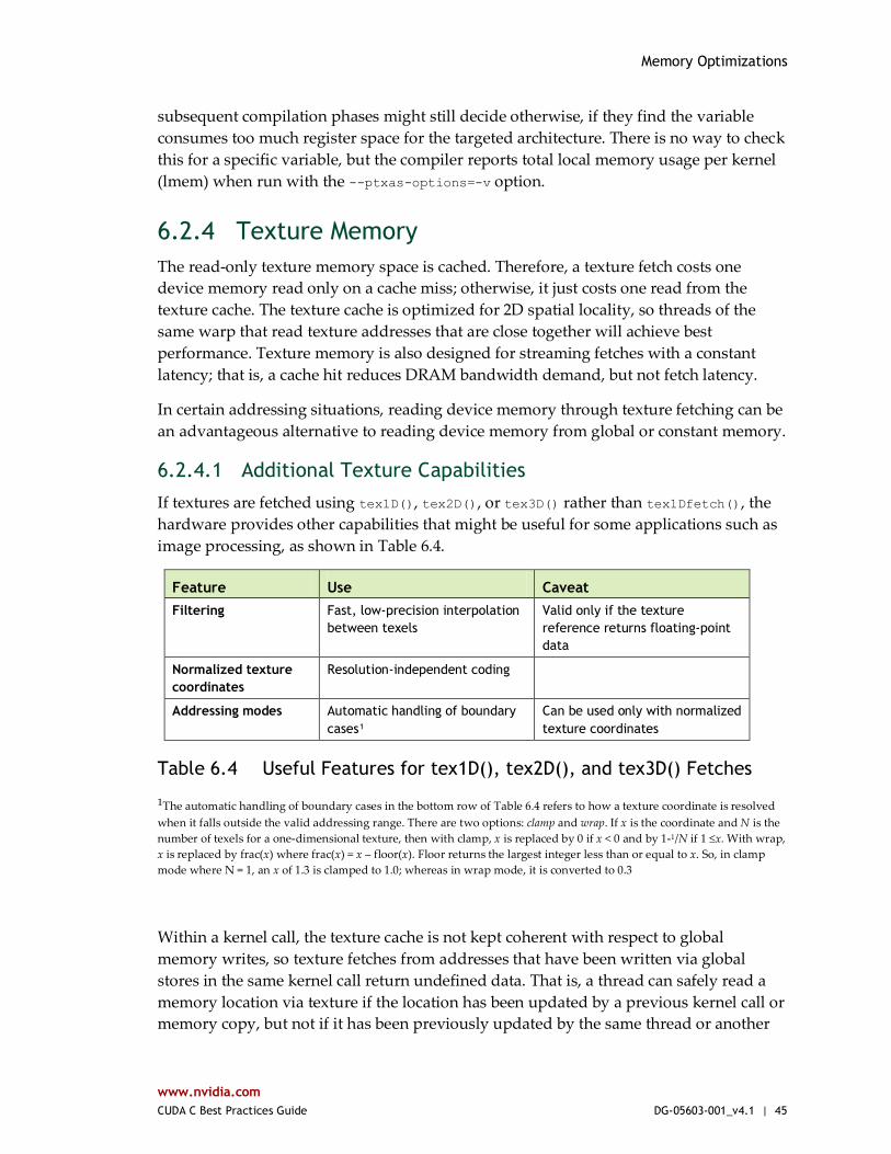
Memory Optimizations
www.nvidia.com
CUDA C Best Practices Guide DG-05603-001_v4.1 | 45
subsequent compilation phases might still decide otherwise, if they find the variable
consumes too much register space for the targeted architecture. There is no way to check
this for a specific variable, but the compiler reports total local memory usage per kernel
(lmem) when run with the --ptxas-options=-v option.
6.2.4 Texture Memory
The read-only texture memory space is cached. Therefore, a texture fetch costs one
device memory read only on a cache miss; otherwise, it just costs one read from the
texture cache. The texture cache is optimized for 2D spatial locality, so threads of the
same warp that read texture addresses that are close together will achieve best
performance. Texture memory is also designed for streaming fetches with a constant
latency; that is, a cache hit reduces DRAM bandwidth demand, but not fetch latency.
In certain addressing situations, reading device memory through texture fetching can be
an advantageous alternative to reading device memory from global or constant memory.
6.2.4.1 Additional Texture Capabilities
If textures are fetched using tex1D(), tex2D(), or tex3D() rather than tex1Dfetch(), the
hardware provides other capabilities that might be useful for some applications such as
image processing, as shown in Table 6.4.
Feature Use Caveat
Filtering Fast, low-precision interpolation
between texels
Valid only if the texture
reference returns floating-point
data
Normalized texture
coordinates
Resolution-independent coding
Addressing modes Automatic handling of boundary
cases¹
Can be used only with normalized
texture coordinates
Table 6.4 Useful Features for tex1D(), tex2D(), and tex3D() Fetches
¹The automatic handling of boundary cases in the bottom row of Table 6.4 refers to how a texture coordinate is resolved
when it falls outside the valid addressing range. There are two options: clamp and wrap. If x is the coordinate and N is the
number of texels for a one-dimensional texture, then with clamp, x is replaced by 0 if x < 0 and by 1-1/N if 1 ≤x. With wrap,
x is replaced by frac(x) where frac(x) = x – floor(x). Floor returns the largest integer less than or equal to x. So, in clamp
mode where N = 1, an x of 1.3 is clamped to 1.0; whereas in wrap mode, it is converted to 0.3
Within a kernel call, the texture cache is not kept coherent with respect to global
memory writes, so texture fetches from addresses that have been written via global
stores in the same kernel call return undefined data. That is, a thread can safely read a
memory location via texture if the location has been updated by a previous kernel call or
memory copy, but not if it has been previously updated by the same thread or another

Memory Optimizations
www.nvidia.com
CUDA C Best Practices Guide DG-05603-001_v4.1 | 46
thread within the same kernel call. This is relevant only when fetching from linear or
pitch-linear memory because a kernel cannot write to CUDA arrays.
6.2.5 Constant Memory
There is a total of 64 KB constant memory on a device. The constant memory space is
cached. As a result, a read from constant memory costs one memory read from device
memory only on a cache miss; otherwise, it just costs one read from the constant cache.
For all threads of a half warp, reading from the constant cache is as fast as reading from
a register as long as all threads read the same address. Accesses to different addresses by
threads within a half warp are serialized, so cost scales linearly with the number of
different addresses read by all threads within a half warp.
Alternatively, on devices of compute capability 2.x, programs use the LoaD Uniform
(LDU) operation; see Section F.4.4 of the CUDA C Programming Guide for details.
6.2.6 Registers
Generally, accessing a register consumes zero extra clock cycles per instruction, but
delays may occur due to register read-after-write dependencies and register memory
bank conflicts.
The latency of read-after-write dependencies is approximately 24 cycles, but this latency
is completely hidden on multiprocessors that have at least 192 active threads (that is, 6
warps) for devices of compute capability 1.x (8 CUDA cores per multiprocessor * 24
cycles of latency = 192 active threads to cover that latency). For devices of compute
capability 2.0, which have 32 CUDA cores per multiprocessor, as many as 768 threads
might be required to completely hide latency.
The compiler and hardware thread scheduler will schedule instructions as optimally as
possible to avoid register memory bank conflicts. They achieve the best results when the
number of threads per block is a multiple of 64. Other than following this rule, an
application has no direct control over these bank conflicts. In particular, there is no
register-related reason to pack data into float4 or int4 types.
6.2.6.1 Register Pressure
Register pressure occurs when there are not enough registers available for a given task.
Even though each multiprocessor contains thousands of 32-bit registers (see Section F.1
of the CUDA C Programming Guide), these are partitioned among concurrent threads. To
prevent the compiler from allocating too many registers, use the –maxrregcount=N
compiler command-line option (see Section B.1 below) or the launch bounds kernel
definition qualifier (see Section B.17 of the CUDA C Programming Guide) to control the
maximum number of registers to allocated per thread.

Memory Optimizations
www.nvidia.com
CUDA C Best Practices Guide DG-05603-001_v4.1 | 47
6.3 ALLOCATION
Device memory allocation and de-allocation via cudaMalloc() and cudaFree() are
expensive operations, so device memory should be reused and/or sub-allocated by the
application wherever possible to minimize the impact of allocations on overall
performance.
www.nvidia.com
CUDA C Best Practices Guide DG-05603-001_v4.1 | 48
Chapter 7. EXECUTION CONFIGURATION OPTIMIZATIONS
One of the keys to good performance is to keep the multiprocessors on the device as
busy as possible. A device in which work is poorly balanced across the multiprocessors
will deliver suboptimal performance. Hence, it’s important to design your application to
use threads and blocks in a way that maximizes hardware utilization and to limit
practices that impede the free distribution of work. A key concept in this effort is
occupancy, which is explained in the following sections.
Another important concept is the management of system resources allocated for a
particular task. How to manage this resource utilization is discussed in the final sections
of this chapter.
7.1 OCCUPANCY
Thread instructions are executed sequentially in CUDA, and, as a result, executing other
warps when one warp is paused or stalled is the only way to hide latencies and keep the
hardware busy. Some metric related to the number of active warps on a multiprocessor
is therefore important in determining how effectively the hardware is kept busy. This
metric is occupancy.
Occupancy is the ratio of the number of active warps per multiprocessor to the
maximum number of possible active warps. (To determine the latter number, see the
deviceQuery code sample in the GPU Computing SDK or refer to Appendix F in the
CUDA C Programming Guide.) Another way to view occupancy is the percentage of the
hardware’s ability to process warps that is actively in use.
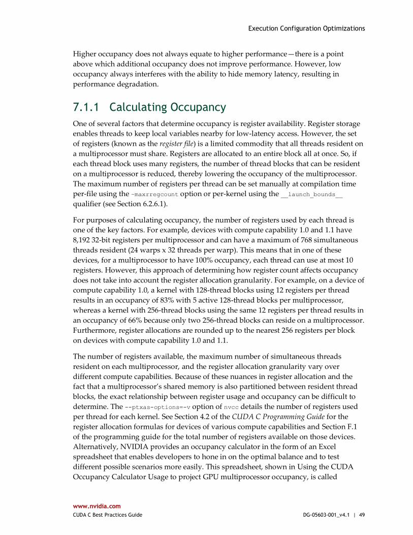
Execution Configuration Optimizations
www.nvidia.com
CUDA C Best Practices Guide DG-05603-001_v4.1 | 49
Higher occupancy does not always equate to higher performance—there is a point
above which additional occupancy does not improve performance. However, low
occupancy always interferes with the ability to hide memory latency, resulting in
performance degradation.
7.1.1 Calculating Occupancy
One of several factors that determine occupancy is register availability. Register storage
enables threads to keep local variables nearby for low-latency access. However, the set
of registers (known as the register file) is a limited commodity that all threads resident on
a multiprocessor must share. Registers are allocated to an entire block all at once. So, if
each thread block uses many registers, the number of thread blocks that can be resident
on a multiprocessor is reduced, thereby lowering the occupancy of the multiprocessor.
The maximum number of registers per thread can be set manually at compilation time
per-file using the –maxrregcount option or per-kernel using the __launch_bounds__
qualifier (see Section 6.2.6.1).
For purposes of calculating occupancy, the number of registers used by each thread is
one of the key factors. For example, devices with compute capability 1.0 and 1.1 have
8,192 32-bit registers per multiprocessor and can have a maximum of 768 simultaneous
threads resident (24 warps x 32 threads per warp). This means that in one of these
devices, for a multiprocessor to have 100% occupancy, each thread can use at most 10
registers. However, this approach of determining how register count affects occupancy
does not take into account the register allocation granularity. For example, on a device of
compute capability 1.0, a kernel with 128-thread blocks using 12 registers per thread
results in an occupancy of 83% with 5 active 128-thread blocks per multiprocessor,
whereas a kernel with 256-thread blocks using the same 12 registers per thread results in
an occupancy of 66% because only two 256-thread blocks can reside on a multiprocessor.
Furthermore, register allocations are rounded up to the nearest 256 registers per block
on devices with compute capability 1.0 and 1.1.
The number of registers available, the maximum number of simultaneous threads
resident on each multiprocessor, and the register allocation granularity vary over
different compute capabilities. Because of these nuances in register allocation and the
fact that a multiprocessor’s shared memory is also partitioned between resident thread
blocks, the exact relationship between register usage and occupancy can be difficult to
determine. The --ptxas-options=-v option of nvcc details the number of registers used
per thread for each kernel. See Section 4.2 of the CUDA C Programming Guide for the
register allocation formulas for devices of various compute capabilities and Section F.1
of the programming guide for the total number of registers available on those devices.
Alternatively, NVIDIA provides an occupancy calculator in the form of an Excel
spreadsheet that enables developers to hone in on the optimal balance and to test
different possible scenarios more easily. This spreadsheet, shown in Using the CUDA
Occupancy Calculator Usage to project GPU multiprocessor occupancy, is called
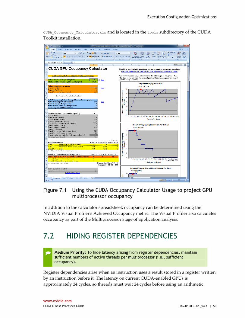
Execution Configuration Optimizations
www.nvidia.com
CUDA C Best Practices Guide DG-05603-001_v4.1 | 50
CUDA_Occupancy_Calculator.xls and is located in the tools subdirectory of the CUDA
Toolkit installation.
Figure 7.1 Using the CUDA Occupancy Calculator Usage to project GPU multiprocessor occupancy
In addition to the calculator spreadsheet, occupancy can be determined using the
NVIDIA Visual Profiler's Achieved Occupancy metric. The Visual Profiler also calculates
occupancy as part of the Multiprocessor stage of application analysis.
7.2 HIDING REGISTER DEPENDENCIES
Medium Priority: To hide latency arising from register dependencies, maintain sufficient numbers of active threads per multiprocessor (i.e., sufficient occupancy).
Register dependencies arise when an instruction uses a result stored in a register written
by an instruction before it. The latency on current CUDA-enabled GPUs is
approximately 24 cycles, so threads must wait 24 cycles before using an arithmetic

Execution Configuration Optimizations
www.nvidia.com
CUDA C Best Practices Guide DG-05603-001_v4.1 | 51
result. However, this latency can be completely hidden by the execution of threads in
other warps. See Section 6.2.6 for details.
7.3 THREAD AND BLOCK HEURISTICS
Medium Priority: The number of threads per block should be a multiple of 32 threads, because this provides optimal computing efficiency and facilitates coalescing.
The dimension and size of blocks per grid and the dimension and size of threads per
block are both important factors. The multidimensional aspect of these parameters
allows easier mapping of multidimensional problems to CUDA and does not play a role
in performance. As a result, this section discusses size but not dimension.
Latency hiding and occupancy depend on the number of active warps per
multiprocessor, which is implicitly determined by the execution parameters along with
resource (register and shared memory) constraints. Choosing execution parameters is a
matter of striking a balance between latency hiding (occupancy) and resource
utilization.
Choosing the execution configuration parameters should be done in tandem; however,
there are certain heuristics that apply to each parameter individually. When choosing
the first execution configuration parameter—the number of blocks per grid, or grid size—
the primary concern is keeping the entire GPU busy. The number of blocks in a grid
should be larger than the number of multiprocessors so that all multiprocessors have at
least one block to execute. Furthermore, there should be multiple active blocks per
multiprocessor so that blocks that aren’t waiting for a __syncthreads() can keep the
hardware busy. This recommendation is subject to resource availability; therefore, it
should be determined in the context of the second execution parameter—the number of
threads per block, or block size—as well as shared memory usage. To scale to future
devices, the number of blocks per kernel launch should be in the thousands.
When choosing the block size, it is important to remember that multiple concurrent
blocks can reside on a multiprocessor, so occupancy is not determined by block size
alone. In particular, a larger block size does not imply a higher occupancy. For example,
on a device of compute capability 1.1 or lower, a kernel with a maximum block size of
512 threads results in an occupancy of 66 percent because the maximum number of
threads per multiprocessor on such a device is 768. Hence, only a single block can be
active per multiprocessor. However, a kernel with 256 threads per block on such a
device can result in 100 percent occupancy with three resident active blocks.
Execution Configuration Optimizations
www.nvidia.com
CUDA C Best Practices Guide DG-05603-001_v4.1 | 52
As mentioned in Section 7.1, higher occupancy does not always equate to better
performance. For example, improving occupancy from 66 percent to 100 percent
generally does not translate to a similar increase in performance. A lower occupancy
kernel will have more registers available per thread than a higher occupancy kernel,
which may result in less register spilling to local memory. Typically, once an occupancy
of 50 percent has been reached, additional increases in occupancy do not translate into
improved performance. It is in some cases possible to fully cover latency with even
fewer warps, notably via instruction-level parallelism (ILP); for discussion, see
http://www.nvidia.com/content/GTC-2010/pdfs/2238_GTC2010.pdf.
There are many such factors involved in selecting block size, and inevitably some
experimentation is required. However, a few rules of thumb should be followed:
Threads per block should be a multiple of warp size to avoid wasting computation
on under-populated warps and to facilitate coalescing.
A minimum of 64 threads per block should be used, and only if there are multiple
concurrent blocks per multiprocessor.
Between 128 and 256 threads per block is a better choice and a good initial range for
experimentation with different block sizes.
Use several (3 to 4) smaller thread blocks rather than one large thread block per
multiprocessor if latency affects performance. This is particularly beneficial to
kernels that frequently call __syncthreads().
Note that when a thread block allocates more registers than are available on a
multiprocessor, the kernel launch fails, as it will when too much shared memory or too
many threads are requested.
7.4 EFFECTS OF SHARED MEMORY
Shared memory can be helpful in several situations, such as helping to coalesce or
eliminate redundant access to global memory. However, it also can act as a constraint on
occupancy. In many cases, the amount of shared memory required by a kernel is related
to the block size that was chosen, but the mapping of threads to shared memory
elements does not need to be one-to-one. For example, it may be desirable to use a 32×32
element shared memory array in a kernel, but because the maximum number of threads
per block is 512, it is not possible to launch a kernel with 32×32 threads per block. In
such cases, kernels with 32×16 or 32×8 threads can be launched with each thread
processing two or four elements, respectively, of the shared memory array. The
approach of using a single thread to process multiple elements of a shared memory
array can be beneficial even if limits such as threads per block are not an issue. This is
because some operations common to each element can be performed by the thread once,
amortizing the cost over the number of shared memory elements processed by the
thread.
Execution Configuration Optimizations
www.nvidia.com
CUDA C Best Practices Guide DG-05603-001_v4.1 | 53
A useful technique to determine the sensitivity of performance to occupancy is through
experimentation with the amount of dynamically allocated shared memory, as specified
in the third parameter of the execution configuration. By simply increasing this
parameter (without modifying the kernel), it is possible to effectively reduce the
occupancy of the kernel and measure its effect on performance.
As mentioned in the previous section, once an occupancy of more than 50 percent has
been reached, it generally does not pay to optimize parameters to obtain higher
occupancy ratios. The previous technique can be used to determine whether such a
plateau has been reached.

www.nvidia.com
CUDA C Best Practices Guide DG-05603-001_v4.1 | 54
Chapter 8. INSTRUCTION OPTIMIZATIONS
Awareness of how instructions are executed often permits low-level optimizations that
can be useful, especially in code that is run frequently (the so-called hot spot in a
program). Best practices suggest that this optimization be performed after all higher-
level optimizations have been completed.
8.1 ARITHMETIC INSTRUCTIONS
Single-precision floats provide the best performance, and their use is highly encouraged.
The throughput of individual arithmetic operations on devices of compute capability 1.x
is detailed in Section F.3 of the CUDA C Programming Guide, and the throughput of
these operations on devices of compute capability 2.x is detailed in Section F.4 of the
programming guide.
8.1.1 Division and Modulo Operations
Low Priority: Use shift operations to avoid expensive division and modulo calculations.
Integer division and modulo operations are particularly costly and should be avoided or
replaced with bitwise operations whenever possible: If n is a power of 2, (i/n) is
equivalent to (i ≫ log2(n)) and (i % n) is equivalent to (i & (n-1)).
The compiler will perform these conversions if n is literal. (For further information, refer
to Chapter 5 of the CUDA C Programming Guide).

Instruction Optimizations
www.nvidia.com
CUDA C Best Practices Guide DG-05603-001_v4.1 | 55
8.1.2 Reciprocal Square Root
The reciprocal square root should always be invoked explicitly as rsqrtf() for single
precision and rsqrt() for double precision. The compiler optimizes 1.0f/sqrtf(x) into
rsqrtf() only when this does not violate IEEE-754 semantics.
8.1.3 Other Arithmetic Instructions
Low Priority: Avoid automatic conversion of doubles to floats.
The compiler must on occasion insert conversion instructions, introducing additional
execution cycles. This is the case for
Functions operating on char or short whose operands generally need to be
converted to an int
Double-precision floating-point constants (defined without any type suffix) used as
input to single-precision floating-point computations
The latter case can be avoided by using single-precision floating-point constants, defined
with an f suffix such as 3.141592653589793f, 1.0f, 0.5f. This suffix has accuracy
implications in addition to its ramifications on performance. The effects on accuracy are
discussed in Section 4.3.3. Note that this distinction is particularly important to
performance on devices of compute capability 2.x.
For single-precision code, use of the float type and the single-precision math functions
are highly recommended. When compiling for devices without native double-precision
support such as devices of compute capability 1.2 and earlier, each double-precision
floating-point variable is converted to single-precision floating-point format (but retains
its size of 64 bits) and double-precision arithmetic is demoted to single-precision
arithmetic.
It should also be noted that the CUDA math library’s complementary error function,
erfcf(), is particularly fast with full single-precision accuracy.
8.1.4 Math Libraries
Medium Priority: Use the fast math library whenever speed trumps precision.
Two types of runtime math operations are supported. They can be distinguished by
their names: some have names with prepended underscores, whereas others do not (e.g.,
__functionName() versus functionName()). Functions following the __functionName()
naming convention map directly to the hardware level. They are faster but provide
somewhat lower accuracy (e.g., __sinf(x) and __expf(x)). Functions following
functionName() naming convention are slower but have higher accuracy (e.g., sinf(x)

Instruction Optimizations
www.nvidia.com
CUDA C Best Practices Guide DG-05603-001_v4.1 | 56
and expf(x)). The throughput of __sinf(x), __cosf(x), and __expf(x) is much greater
than that of sinf(x), cosf(x), tanf(x). The latter become even more expensive (about
an order of magnitude slower) if the magnitude of the argument x needs to be reduced.
Moreover, in such cases, the argument-reduction code uses local memory, which can
affect performance even more because of the high latency of local memory. More details
are available in the CUDA C Programming Guide.
Note also that whenever sine and cosine of the same argument are computed, the
sincos… family of instructions should be used to optimize performance:
sincosf() for single-precision fast math (see next paragraph)
sincosf() for regular single-precision
sincos() for double precision
The –use_fast_math compiler option of nvcc coerces every functionName() call to the
equivalent __functionName() call. This switch should be used whenever accuracy is a
lesser priority than the performance. This is frequently the case with transcendental
functions. Note this switch is effective only on single-precision floating point.
Medium Priority: Prefer faster, more specialized math functions over slower, more general ones when possible.
For small integer powers (e.g., x2 or x3), explicit multiplication is almost certainly faster
than the use of general exponentiation routines such as pow(). While compiler
optimization improvements continually seek to narrow this gap, explicit multiplication
(or the use of an equivalent purpose-built inline function or macro) can have a
significant advantage. This advantage is increased when several powers of the same
base are needed (e.g., where both x2 and x5 are calculated in close proximity), as this aids
the compiler in its common sub-expression elimination (CSE) optimization.
For exponentiation using base 2 or 10, use the functions exp2() or expf2() and exp10()
or expf10() rather than the functions pow() or powf(). Both pow() and powf() are heavy-
weight functions in terms of register pressure and instruction count due to the
numerous special cases arising in general exponentiation and the difficulty of achieving
good accuracy across the entire ranges of the base and the exponent. The functions
exp2(), exp2f(), exp10(), and exp10f(), on the other hand, are similar to exp() and
expf() in terms of performance, and can be as much as ten times faster than their
pow()/powf() equivalents.
For exponentiation with an exponent of 1/3, use the cbrt() or cbrtf() function rather
than the generic exponentiation functions pow() or powf(), as the former are significantly
faster than the latter. Likewise, for exponentation with an exponent of -1/3, use rcbrt()
or rcbrtf().
Replace sin(π*<expr>) with sinpi(<expr>) and cos(π*<expr>) with cospi(<expr>). This
is advantageous with regard to both accuracy and performance. As a particular example,

Instruction Optimizations
www.nvidia.com
CUDA C Best Practices Guide DG-05603-001_v4.1 | 57
to evaluate the sine function in degrees instead of radians, use sinpi(x/180.0).
Similarly, the single-precision functions sinpif() and cospif() should replace calls to
sinf() and cosf() when the function argument is of the form π*<expr>. (The
performance advantage sinpi() has over sin() is due to simplified argument reduction;
the accuracy advantage is because sinpi() multiplies by π only implicitly, effectively
using an infinitely precise mathematical π rather than a single- or double-precision
approximation thereof.)
8.1.5 Precision-related Compiler Flags
By default, the nvcc compiler generates IEEE-compliant code for devices of compute
capability 2.x, but it also provides options to generate code that somewhat less accurate
but faster and that is closer to the code generated for earlier devices:
-ftz=true (denormalized numbers are flushed to zero)
-prec-div=false (less precise division)
-prec-sqrt=false (less precise square root)
Another, more aggressive, option is -use_fast_math, which coerces every
functionName() call to the equivalent __functionName() call. This makes the code run
faster at the cost of diminished precision and accuracy. See Section 8.1.4.
8.2 MEMORY INSTRUCTIONS
High Priority: Minimize the use of global memory. Prefer shared memory access where possible.
Memory instructions include any instruction that reads from or writes to shared, local,
or global memory. When accessing uncached local or global memory, there are 400 to
600 clock cycles of memory latency.
As an example, the assignment operator in the following sample code has a high
throughput, but, crucially, there is a latency of 400 to 600 clock cycles to read data from
global memory:
__shared__ float shared[32];
__device__ float device[32];
shared[threadIdx.x] = device[threadIdx.x];
Much of this global memory latency can be hidden by the thread scheduler if there are
sufficient independent arithmetic instructions that can be issued while waiting for the
global memory access to complete. However, it is best to avoid accessing global memory
whenever possible.
www.nvidia.com
CUDA C Best Practices Guide DG-05603-001_v4.1 | 58
Chapter 9. CONTROL FLOW
9.1 BRANCHING AND DIVERGENCE
High Priority: Avoid different execution paths within the same warp.
Any flow control instruction (if, switch, do, for, while) can significantly affect the
instruction throughput by causing threads of the same warp to diverge; that is, to follow
different execution paths. If this happens, the different execution paths must be
serialized, since all of the threads of a warp share a program counter; this increases the
total number of instructions executed for this warp. When all the different execution
paths have completed, the threads converge back to the same execution path.
To obtain best performance in cases where the control flow depends on the thread ID,
the controlling condition should be written so as to minimize the number of divergent
warps.
This is possible because the distribution of the warps across the block is deterministic as
mentioned in Section 4.1 of the CUDA C Programming Guide. A trivial example is when
the controlling condition depends only on (threadIdx / WSIZE) where WSIZE is the warp
size.
In this case, no warp diverges because the controlling condition is perfectly aligned with
the warps.
Control Flow
www.nvidia.com
CUDA C Best Practices Guide DG-05603-001_v4.1 | 59
9.2 BRANCH PREDICATION
Low Priority: Make it easy for the compiler to use branch predication in lieu of loops or control statements.
Sometimes, the compiler may unroll loops or optimize out if or switch statements by
using branch predication instead. In these cases, no warp can ever diverge. The
programmer can also control loop unrolling using
#pragma unroll
For more information on this pragma, refer to the CUDA C Programming Guide.
When using branch predication, none of the instructions whose execution depends on
the controlling condition is skipped. Instead, each such instruction is associated with a
per-thread condition code or predicate that is set to true or false according to the
controlling condition. Although each of these instructions is scheduled for execution,
only the instructions with a true predicate are actually executed. Instructions with a false
predicate do not write results, and they also do not evaluate addresses or read operands.
The compiler replaces a branch instruction with predicated instructions only if the
number of instructions controlled by the branch condition is less than or equal to a
certain threshold: If the compiler determines that the condition is likely to produce
many divergent warps, this threshold is 7; otherwise it is 4.
9.3 LOOP COUNTERS SIGNED VS. UNSIGNED
Medium Priority: Use signed integers rather than unsigned integers as loop counters.
In the C language standard, unsigned integer overflow semantics are well defined,
whereas signed integer overflow causes undefined results. Therefore, the compiler can
optimize more aggressively with signed arithmetic than it can with unsigned arithmetic.
This is of particular note with loop counters: since it is common for loop counters to
have values that are always positive, it may be tempting to declare the counters as
unsigned. For slightly better performance, however, they should instead be declared as
signed.
For example, consider the following code:
for (i = 0; i < n; i++) {
out[i] = in[offset + stride*i];
}

Control Flow
www.nvidia.com
CUDA C Best Practices Guide DG-05603-001_v4.1 | 60
Here, the sub-expression stride*i could overflow a 32-bit integer, so if i is declared as
unsigned, the overflow semantics prevent the compiler from using some optimizations
that might otherwise have applied, such as strength reduction. If instead i is declared as
signed, where the overflow semantics are undefined, the compiler has more leeway to
use these optimizations.

www.nvidia.com
CUDA C Best Practices Guide DG-05603-001_v4.1 | 61
DEPLOYING CUDA APPLICATIONS
Having completed the GPU acceleration of one or more components of the application it
is possible to compare the outcome with the original expectation. Recall that the initial
assess step allowed the developer to determine an upper bound for the potential
speedup attainable by accelerating given hotspots.
Before tackling other hotspots to improve the total speedup, the developer should
consider taking the partially parallelized implementation and carry it through to
production. This is important for a number of reasons; for example, it allows the user to
profit from their investment as early as possible (the speedup may be partial but is still
valuable), and it minimizes risk for the developer and the user by providing an
evolutionary rather than revolutionary set of changes to the application.
www.nvidia.com
CUDA C Best Practices Guide DG-05603-001_v4.1 | 62
Chapter 10. UNDERSTANDING THE PROGRAMMING ENVIRONMENT
With each generation of NVIDIA processors, new features are added to the GPU that
CUDA can leverage. Consequently, it’s important to understand the characteristics of
the architecture.
Programmers should be aware of two version numbers. The first is the compute
capability, and the second is the version number of the CUDA Runtime and CUDA
Driver APIs.
10.1 CUDA COMPUTE CAPABILITY
The compute capability describes the features of the hardware and reflects the set of
instructions supported by the device as well as other specifications, such as the
maximum number of threads per block and the number of registers per multiprocessor.
Higher compute capability versions are supersets of lower (that is, earlier) versions, so
they are backward compatible.
The compute capability of the GPU in the device can be queried programmatically as
illustrated in the NVIDIA GPU Computing SDK in the deviceQuery sample. The output
for that program is shown in Figure 10.1. This information is obtained by calling
cudaGetDeviceProperties() and accessing the information in the structure it returns.
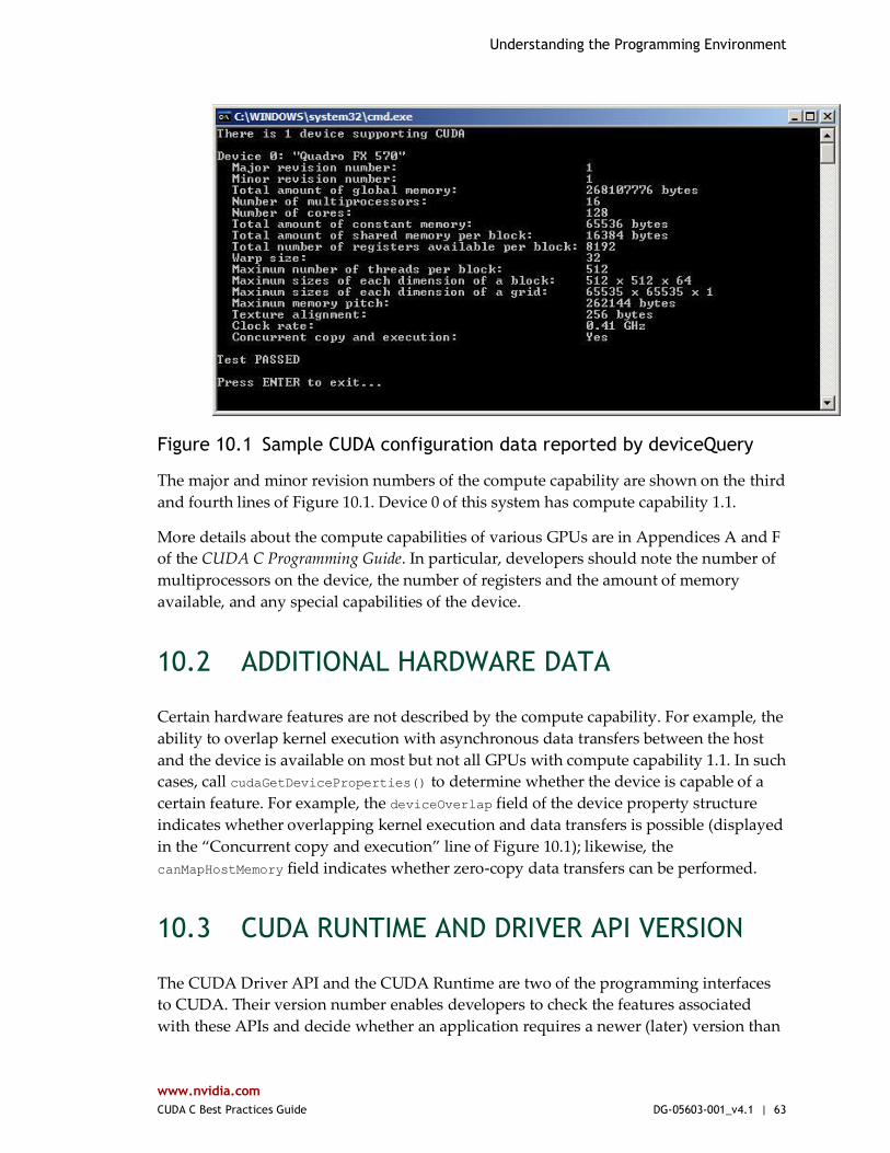
Understanding the Programming Environment
www.nvidia.com
CUDA C Best Practices Guide DG-05603-001_v4.1 | 63
Figure 10.1 Sample CUDA configuration data reported by deviceQuery
The major and minor revision numbers of the compute capability are shown on the third
and fourth lines of Figure 10.1. Device 0 of this system has compute capability 1.1.
More details about the compute capabilities of various GPUs are in Appendices A and F
of the CUDA C Programming Guide. In particular, developers should note the number of
multiprocessors on the device, the number of registers and the amount of memory
available, and any special capabilities of the device.
10.2 ADDITIONAL HARDWARE DATA
Certain hardware features are not described by the compute capability. For example, the
ability to overlap kernel execution with asynchronous data transfers between the host
and the device is available on most but not all GPUs with compute capability 1.1. In such
cases, call cudaGetDeviceProperties() to determine whether the device is capable of a
certain feature. For example, the deviceOverlap field of the device property structure
indicates whether overlapping kernel execution and data transfers is possible (displayed
in the “Concurrent copy and execution” line of Figure 10.1); likewise, the
canMapHostMemory field indicates whether zero-copy data transfers can be performed.
10.3 CUDA RUNTIME AND DRIVER API VERSION
The CUDA Driver API and the CUDA Runtime are two of the programming interfaces
to CUDA. Their version number enables developers to check the features associated
with these APIs and decide whether an application requires a newer (later) version than

Understanding the Programming Environment
www.nvidia.com
CUDA C Best Practices Guide DG-05603-001_v4.1 | 64
the one currently installed. This is important because the CUDA Driver API is backward
compatible but not forward compatible, meaning that applications, plug-ins, and libraries
(including the CUDA Runtime) compiled against a particular version of the Driver API
will continue to work on subsequent (later) driver releases. However, applications, plug-
ins, and libraries (including the CUDA Runtime) compiled against a particular version
of the Driver API may not work on earlier versions of the driver, as illustrated in Figure
10.2.
1.0
Driver
Apps,
Libs &
Plug-ins
1.1
Driver
Apps,
Libs &
Plug-ins
2.0
Driver
Apps,
Libs &
Plug-ins
Compatible Incompatible
...
...
Figure 10.2 Compatibility of CUDA versions
10.4 WHICH COMPUTE CAPABILITY TO TARGET
When in doubt about the compute capability of the hardware that will be present at
runtime, it is best to assume a compute capability of 1.0 as defined in the CUDA C
Programming Guide, Section F.1, or a compute capability of 1.3 if double-precision
arithmetic is required.
To target specific versions of NVIDIA hardware and CUDA software, use the
–arch, -code, and –gencode options of nvcc. Code that contains double-precision
arithmetic, for example, must be compiled with “-arch=sm_13” (or higher compute
capability), otherwise double-precision arithmetic will get demoted to single-precision
arithmetic (see Section 4.3.3). This and other compiler switches are discussed further in
Appendix B.

Understanding the Programming Environment
www.nvidia.com
CUDA C Best Practices Guide DG-05603-001_v4.1 | 65
10.5 CUDA RUNTIME
The host runtime component of the CUDA software environment can be used only by
host functions. It provides functions to handle the following:
Device management
Context management
Memory management
Code module management
Execution control
Texture reference management
Interoperability with OpenGL and Direct3D
As compared to the lower-level CUDA Driver API, the CUDA Runtime greatly eases
device management by providing implicit initialization, context management, and
device code module management. The C/C++ host code generated by nvcc utilizes the
CUDA Runtime, so applications that link to this code will depend on the CUDA
Runtime; similarly, any code that uses the cuBLAS, cuFFT, and other CUDA Toolkit
libraries will also depend on the CUDA Runtime, which is used internally by these
libraries.
The functions that make up the CUDA Runtime API are explained in the CUDA Toolkit
Reference Manual.
The CUDA Runtime handles kernel loading and setting up kernel parameters and
launch configuration before the kernel is launched. The implicit driver version checking,
code initialization, CUDA context management, CUDA module management (cubin to
function mapping), kernel configuration, and parameter passing are all performed by
the CUDA Runtime.
It comprises two principal parts:
A C-style function interface (cuda_runtime_api.h).
C++-style convenience wrappers (cuda_runtime.h) built on top of the C-style
functions.
For more information on the Runtime API, refer to Section 3.2 of the CUDA C
Programming Guide.

www.nvidia.com
CUDA C Best Practices Guide DG-05603-001_v4.1 | 66
Chapter 11. PREPARING THE APPLICATION FOR DEPLOYMENT
11.1 ERROR HANDLING
All CUDA Runtime API calls return an error code of type cudaError_t; the return value
will be equal to cudaSuccess if no errors have occurred. (The exceptions to this are kernel
launches, which return void, and cudaGetErrorString(), which returns a character string
describing the cudaError_t code that was passed into it.) The CUDA Toolkit libraries
(cuBLAS, cuFFT, etc.) likewise return their own sets of error codes.
Since some CUDA API calls and all kernel launches are asynchronous with respect to
the host code, errors may be reported to the host asynchronously as well; often this
occurs the next time the host and device synchronize with each other, such as during a
call to cudaMemcpy() or to cudaDeviceSynchronize().
Always check the error return values on all CUDA API functions, even for functions that
are not expected to fail, as this will allow the application to detect and recover from
errors as soon as possible should they occur. Applications that do not check for CUDA
API errors could at times run to completion without having noticed that the data
calculated by the GPU is incomplete, invalid, or uninitialized.
11.2 DISTRIBUTING THE CUDA RUNTIME AND LIBRARIES
The CUDA Toolkit’s end-user license agreement (EULA) allows for redistribution of
many of the CUDA libraries under certain terms and conditions.
Preparing the Application for Deployment
www.nvidia.com
CUDA C Best Practices Guide DG-05603-001_v4.1 | 67
This allows applications that depend on these libraries to redistribute the exact versions
of the libraries against which they were built and tested, thereby avoiding any trouble
for end users who might have a different version of the CUDA Toolkit (or perhaps none
at all) installed on their machines.
Please refer to the EULA for details.
Note: this does not apply to the NVIDIA driver; the end user must still download and
install an NVIDIA driver appropriate to their GPU(s) and operating system.
www.nvidia.com
CUDA C Best Practices Guide DG-05603-001_v4.1 | 68
Chapter 12. DEPLOYMENT INFRASTRUCTURE TOOLS
12.1 NVIDIA-SMI
The NVIDIA System Management Interface (nvidia-smi) is a command line utility that
aids in the management and monitoring of NVIDIA GPU devices. This utility allows
administrators to query GPU device state and, with the appropriate privileges, permits
administrators to modify GPU device state. nvidia-smi is targeted at Tesla and certain
Quadro GPUs, though limited support is also available on other NVIDIA GPUs.
nvidia-smi ships with NVIDIA GPU display drivers on Linux, and with 64-bit Windows
Server 2008 R2 and Windows 7. nvidia-smi can output queried information as XML or
as human-readable plain text either to standard output or to a file. See the nvidia-smi
documenation for details. Please note that new versions of nvidia-smi are not
guaranteed to be backward-compatible with previous versions.
12.1.1 Queryable state ECC error counts. Both correctable single-bit and detectable double-bit errors are
reported. Error counts are provided for both the current boot cycle and the lifetime
of the GPU.
GPU utilization. Current utilization rates are reported for both the compute
resources of the GPU and the memory interface.
Active compute process. The list of active processes running on the GPU is reported,
along with the corresponding process name/ID and allocated GPU memory.
Clocks and performance state. Max and current clock rates are reported for several
important clock domains, as well as the current GPU performance state (pstate).
Temperature and fan speed. The current GPU core temperature is reported, along
with fan speeds for products with active cooling.
Deployment Infrastructure Tools
www.nvidia.com
CUDA C Best Practices Guide DG-05603-001_v4.1 | 69
Power management. The current board power draw and power limits are reported
for products that report these measurements.
Identification. Various dynamic and static information is reported, including board
serial numbers, PCI device IDs, VBIOS/Inforom version numbers and product
names.
12.1.2 Modifiable state ECC mode. Enable and disable ECC reporting.
ECC reset. Clear single- and double-bit ECC error counts.
Compute mode. Indicate whether compute processes can run on the GPU and
whether they run exclusively or concurrently with other compute processes.
Persistence mode. Indicate whether the NVIDIA driver stays loaded when no
applications are connected to the GPU. It is best to enable this option in most
circumstances.
GPU reset. Reinitialize the GPU hardware and software state via a secondary bus
reset.
12.2 NVML
The NVIDIA Management Library (NVML) is a C-based interface that provides direct
access to the queries and commands exposed via nvidia-smi intended as a platform for
building 3rd-party system management applications. The NVML API is available on the
NVIDIA developer website as part of the Tesla Deployment Kit through a single header
file and is accompanied by PDF documentation, stub libraries, and sample applications;
see http://developer.nvidia.com/tesla-deployment-kit. Each new version of NVML is
backward-compatible.
An additional set of Perl and Python bindings are provided for the NVML API. These
bindings expose the same features as the C-based interface and also provide backwards
compatibility. The Perl bindings are provided via CPAN and the Python bindings via
PyPI.
All of these products (nvidia-smi, NVML, and the NVML language bindings) are
updated with each new CUDA release and provide roughly the same functionality.
See http://developer.nvidia.com/nvidia-management-library-nvml for additional
information.

Deployment Infrastructure Tools
www.nvidia.com
CUDA C Best Practices Guide DG-05603-001_v4.1 | 70
12.3 CLUSTER MANAGEMENT TOOLS
Managing your GPU cluster will help achieve maximum GPU utilization and help you
and your users extract the best possible performance. Many of the industry’s most
popular cluster management tools now support CUDA GPUs via NVML. For a listing of
some of these tools, see http://developer.nvidia.com/cluster-management.
12.4 COMPILER JIT CACHE MANAGEMENT
Any PTX device code loaded by an application at runtime is compiled further to binary
code by the device driver. This is called just-in-time compilation (JIT). Just-in-time
compilation increases application load time but allows applications to benefit from latest
compiler improvements. It is also the only way for applications to run on devices that
did not exist at the time the application was compiled.
When JIT compilation of PTX device code is used, the NVIDIA driver caches the
resulting binary code on disk. Some aspects of this behavior such as cache location and
maximum cache size can be controlled via the use of environment variables; see Section
3.1.1.2 of the CUDA C Programming Guide.
12.5 CUDA_VISIBLE_DEVICES
It is possible to rearrange the collection of installed CUDA devices that will visible to
and enumerated by a CUDA application prior to the start of that application by way of
the CUDA_VISIBLE_DEVICES environment variable.
Devices to be made visible to the application should be included as a comma-separated
list in terms of the system-wide list of enumerable devices. For example, to use only
devices 0 and 2 from the system-wide list of devices, set CUDA_VISIBLE_DEVICES=0,2
before launching the application. The application will then enumerate these devices as
device 0 and device 1, respectively.
www.nvidia.com
CUDA C Best Practices Guide DG-05603-001_v4.1 | 71
Appendix A. RECOMMENDATIONS AND BEST PRACTICES
This appendix contains a summary of the recommendations for optimization that are
explained in this document.
A.1 Overall Performance Optimization Strategies
Performance optimization revolves around three basic strategies:
Maximizing parallel execution
Optimizing memory usage to achieve maximum memory bandwidth
Optimizing instruction usage to achieve maximum instruction throughput
Maximizing parallel execution starts with structuring the algorithm in a way that
exposes as much data parallelism as possible. Once the parallelism of the algorithm has
been exposed, it needs to be mapped to the hardware as efficiently as possible. This is
done by carefully choosing the execution configuration of each kernel launch. The
application should also maximize parallel execution at a higher level by explicitly
exposing concurrent execution on the device through streams, as well as maximizing
concurrent execution between the host and the device.
Optimizing memory usage starts with minimizing data transfers between the host and
the device because those transfers have much lower bandwidth than internal device data
transfers. Kernel access to global memory also should be minimized by maximizing the
use of shared memory on the device. Sometimes, the best optimization might even be to
avoid any data transfer in the first place by simply recomputing the data whenever it is
needed.
Deployment Infrastructure Tools
www.nvidia.com
CUDA C Best Practices Guide DG-05603-001_v4.1 | 72
The effective bandwidth can vary by an order of magnitude depending on the access
pattern for each type of memory. The next step in optimizing memory usage is therefore
to organize memory accesses according to the optimal memory access patterns. This
optimization is especially important for global memory accesses, because latency of
access costs hundreds of clock cycles. Shared memory accesses, in counterpoint, are
usually worth optimizing only when there exists a high degree of bank conflicts.
As for optimizing instruction usage, the use of arithmetic instructions that have low
throughput should be avoided. This suggests trading precision for speed when it does
not affect the end result, such as using intrinsics instead of regular functions or single
precision instead of double precision. Finally, particular attention must be paid to
control flow instructions due to the SIMT (single instruction multiple thread) nature of
the device.
www.nvidia.com
CUDA C Best Practices Guide DG-05603-001_v4.1 | 73
Appendix B. NVCC COMPILER SWITCHES
B.1 NVCC
The NVIDIA nvcc compiler driver converts .cu files into C for the host system and
CUDA assembly or binary instructions for the device. It supports a number of
command-line parameters, of which the following are especially useful for optimization
and related best practices:
-arch=sm_13 or higher is required for double precision. See Section 4.3.3.
–maxrregcount=N specifies the maximum number of registers kernels can use at a per-
file level. See Section 6.2.6.1. (See also the __launch_bounds__ qualifier discussed in
Section B.17 of the CUDA C Programming Guide to control the number of registers
used on a per-kernel basis.)
--ptxas-options=-v or -Xptxas=-v lists per-kernel register, shared, and constant
memory usage.
-ftz=true (denormalized numbers are flushed to zero)
-prec-div=false (less precise division)
-prec-sqrt=false (less precise square root)
-use_fast_math compiler option of nvcc coerces every functionName() call to the
equivalent __functionName() call. This makes the code run faster at the cost of
diminished precision and accuracy. See Section 8.1.4.
www.nvidia.com
CUDA C Best Practices Guide DG-05603-001_v4.1 | 74
Appendix C. REVISION HISTORY
C.1 Version 4.1
Rearranged the entire guide based on the Assess, Parallelize, Optimize, Deploy
pattern.
www.nvidia.com
Notice
ALL NVIDIA DESIGN SPECIFICATIONS, REFERENCE BOARDS, FILES, DRAWINGS, DIAGNOSTICS, LISTS, AND OTHER
DOCUMENTS (TOGETHER AND SEPARATELY, “MATERIALS”) ARE BEING PROVIDED “AS IS.” NVIDIA MAKES NO WARRANTIES, EXPRESSED, IMPLIED, STATUTORY, OR OTHERWISE WITH RESPECT TO THE MATERIALS, AND
EXPRESSLY DISCLAIMS ALL IMPLIED WARRANTIES OF NONINFRINGEMENT, MERCHANTABILITY, AND FITNESS FOR
A PARTICULAR PURPOSE.
Information furnished is believed to be accurate and reliable. However, NVIDIA Corporation assumes no
responsibility for the consequences of use of such information or for any infringement of patents or other rights of third parties that may result from its use. No license is granted by implication of otherwise under
any patent rights of NVIDIA Corporation. Specifications mentioned in this publication are subject to change
without notice. This publication supersedes and replaces all other information previously supplied. NVIDIA Corporation products are not authorized as critical components in life support devices or systems without
express written approval of NVIDIA Corporation.
Trademarks
NVIDIA and the NVIDIA logo are trademarks or registered trademarks of NVIDIA Corporation in the U.S. and other countries. Other company and product names may be trademarks of the respective companies with
which they are associated.
Copyright
© 2012 NVIDIA Corporation. All rights reserved.