CROSSING CORRIDORS: WILDLIFE USE OF JUMPOUTS AND
UNDERCROSSINGS ALONG A HIGHWAY WITH
WILDLIFE EXCLUSION FENCING
A Thesis
presented to
the Faculty of California Polytechnic State University,
San Luis Obispo
In Partial Fulfillment
of the Requirements for the Degree
Master of Science in Biology
by
Alex Joseph Jensen
August 2018

ii
© 2018
Alex Joseph Jensen
ALL RIGHTS RESERVED

iii
COMMITTEE MEMBERSHIP
TITLE:
AUTHOR:
DATE SUBMITTED:
COMMITTEE CHAIR:
COMMITTEE MEMBER:
COMMITTEE MEMBER:
COMMITTEE MEMBER:
Crossing Corridors: Wildlife use of
jumpouts and undercrossings along a
highway with wildlife exclusion fencing
Alex Joseph Jensen
August 2018
John Perrine, Ph.D.
Associate Professor of Biological Sciences
Clinton Francis, PhD
Assistant Professor of Biological Sciences
Andrew Schaffner, PhD
Professor of Statistics
Anthony Giordano, PhD
Executive Director & President of
S.P.E.C.I.E.S

iv
ABSTRACT
Crossing Corridors: Wildlife use of jumpouts and undercrossings along a highway with
wildlife exclusion fencing
Alex Joseph Jensen
Roads pose two central problems for wildlife: wildlife-vehicle collisions (WVCs) and
habitat fragmentation. Wildlife exclusion fencing can reduce WVCs but can exacerbate
fragmentation. In Chapter 1, I summarize the relevant studies addressing these two
problems, with a focus on large mammals in North America. Chapters 2 and 3 summarize
field assessments of technologies to reduce WVCs and maintain connectivity, specifically
jumpout ramps and underpasses, along Highway 101 near San Luis Obispo, CA. In a
fenced highway, some animals inevitably breach the fence and become trapped, which
increases the risk of a wildlife-vehicle collision. Earthen escape ramps, or “jumpouts”,
can allow the trapped animal to escape the highway corridor. Few studies have quantified
wildlife use of jumpouts, and none for >2 years. We used wildlife cameras to quantify
wildlife use of 4 jumpouts from 2012-2017. Mule deer were 88% percent of our
detections and jumped out 20% of the time. After accounting for pseudoreplication, 33%
of the events were independent events, and 2 groups of deer accounted for 41% of all
detections at the top of the jumpout. Female deer were 86% of the detections and were
much more likely than males to return to the jumpout multiple times. This is the first
study to document use of jumpouts for more than 3 years, the first to account for
pseudoreplication, and the first to quantify differences in jumpout use between male and
female mule deer. We recommend a jumpout height between 1.75m-2m for mule deer to
increase the jumpout success rate. Chapter 3 addresses factors that may affect the use of
undercrossings by mule deer and other wildlife. Wildlife crossings combined with

v
wildlife exclusion fencing have been shown to be the most effective method to reduce
wildlife-vehicle collisions while maintaining ecological connectivity. Although several
studies have quantified wildlife use of undercrossings, very few have exceeded 24
months, and the factors affecting carnivores use of the undercrossings remain unclear.
We quantified mule deer, black bear, mountain lion, and bobcat use of 11 undercrossings
along Highway 101 near San Luis Obispo, California from 2012-2017. We constructed
zero-inflated Poisson general linear models on the monthly activity of our focal species
using underpass dimensionality, distance to cover, substrate, human activity, and location
relative to the wildlife exclusion fence as predictor variables. We accounted for temporal
variation, as well as spatial variation by quantifying the landscape resistance near each
undercrossing. We found that deer almost exclusively used the larger underpasses
whereas the carnivores were considerably less selective. Bears used undercrossings more
that were within the wildlife exclusion fence, whereas mountain lion activity was higher
outside the wildlife exclusion fence. Bobcat activity was highest and most widespread,
and was negatively associated with distance to cover. Regional connectivity is most
important for bear and mountain lion, and the surrounding habitat may be the most
important predictor for their use of undercrossings. We recommend placing GPS collars
on our focal species to more clearly document fine-scale habitat selection near the
highway.
vi
ACKNOWLEDGMENTS
I would like to thank our collaborators at California Department of
Transportation, Nancy Siepel and Morgan Robertson, for their field assistance and
flexibility in taking me on as a volunteer. I appreciate Doug Brewster’s technical
expertise in helping set up our cameras in the undercrossings underneath Highway 101. I
am grateful for the HOURS of time Cal Poly and Allan Hancock undergraduates devoted
to field work and entering data, notably Sofia Carrillo, Gennesee Garcia, Maddie Stukan,
and Mason Dubois. A big shout out to the staff in the Biological Sciences department:
Kristin Reeves, Ellen Calcagno, and Melanie Gutierrez. I appreciate my committee for
their guidance; thank you to Andrew Schaffner for his statistical expertise, and Clinton
Francis and Anthony Giordano for their valuable feedback and advice. Thank you most
of all to my advisor, Dr. John Perrine. He has helped me become a better scientist, as well
as a better writer. I appreciate the time and energy he invested in me during this process.

vii
TABLE OF CONTENTS
Page
LIST OF TABLES…………………………………………………………………...……x
LIST OF FIGURES…………………………………………………………………...….xii
CHAPTER
1. LITERATURE REVIEW……………………………………………………………….1
1.1 Introduction……………………………………………………………………1
1.2 Part 1: How Roads Affect Wildlife………………….…………………………2
1.2.a Direct effects: Wildlife-Vehicle Collisions…………………………..3
1.2.a.i Temporal variation……………………………………...….4
1.2.a.ii Human health and economics……………………………..6
1.2.b Indirect effects………………………………………………………6
1.3 Part 2: Mitigation……………………………………………………………..10
1.3.a Wildlife exclusion fencing………………………………………….10
1.3.b Jumpouts………………………………………………………...…11
1.3.c Wildlife crossings…………………………………………………..14
1.3.c.i Dimensionality……………………………………………16
1.3.c.ii Human dimensionality……………………………..…….17
1.3.c.iii Temporal and spatial variation………………………..…18
1.3.c.iv Adaptation time…………………………………….……19
1.3.c.v Community interactions…………………………….……19
1.3.c.vi Other factors…………………………..…………………20
2. WILDLIFE USE OF JUMPOUTS………………………………...………….……….23
viii
2.1 Introduction…………………………………………………………………..23
2.2 Methods………………………………………………………………………26
2.2.a Study site………………………………………………………...…26
2.2.b Data collection…………………………………………………...…27
2.2.c Data analysis…………………………………………………..……27
2.3 Results………………………………………………………………………..29
2.4 Discussion……………………………………………………………………33
2.4.a Group dynamics……………………………………………………37
2.4.b Deer behavior………………………………………………………38
2.4.c Management implications…………………………………………..39
3. WILDLIFE USE OF UNDERCROSSINGS………………………………………….52
3.1 Introduction…………………………………………………………………..52
3.2 Methods………………………………………………………………………55
3.2.a Study site…………………………………………………………...55
3.2.b Data collection………………………………………………...……56
3.2.c Data analysis………………………………………………..………57
3.3 Results………………………………………………………………………..62
3.3.a Landscape resistance…………………………………………….....63
3.3.b Dimensionality……………………………………………..………63
3.3.c Distance to cover and substrate…………………………………….64
3.3.d Fencing and human activity………………………………………..64
3.4 Discussion……………………………………………………………………65
3.4.a Deer…………………………………………………………...……65

ix
3.4.b Bear………………………………………………………………...67
3.4.c Mountain lion………………………………………………………69
3.4.d Bobcat…………………………………………………………..….71
3.4.e Next steps…………………………………………………………..72
3.4.f Management implications…………………………………………..72
4. REFERENCES…………………………………………………………..…………….89
x
LIST OF TABLES
Table Page
Table 2.1: Camera performance across all 4 sites. “Day active only” indicates
that the camera was not functional at night due to flash failure.…………...……….……..41
Table 2.2: The number (%) of detection events per species by site. These
numbers are irrespective of group size.…………………………………...……….....…...42
Table 2.3: Number (%) of deer detection events by site. 4 different outcomes
relative to the wildlife exclusion fence: II means approached from inside and
stayed inside (did not jump out), IO means approached from inside and
went outside (jumped out), OO means approached the jumpout from outside
and stayed outside, I? means the event started on the inside (on top of the
jumpout ramp) but the outcome was ambiguous, and OI means approached
the jumpout from outside and jumped in...…………………………………...………..….43
Table 2.4: Outcomes of events that began at the top of the jumpout ramp for
male and female deer. II means approached from inside and stayed inside (did
not jump out), and IO means approached from inside and went outside (jumped
out). Detections during the months of February, March, and April were removed..……...44
Table 2.5: Initial outcomes and jumpout ratios of 10 groups of deer detected
multiple times. Groups A-F are composed of females and juveniles that were
detected at least 10 times, groups G-J have a male deer in the group and
were detected multiple times. IO indicates events where the group successfully
jumped out.…………………………………………………………………………..…...45
Table 3.1: Total survey effort for each site, including monitoring time frame.…….…...75
Table 3.2a: Undercrossing attributes: dimensionality and distance to cover.
Openness is (width*height)/length. SB indicates the undercrossing entrance
on the southbound side of the highway, NB indicates the northbound side, and
Avg. is the average of the two.……………………………………………………..……76
Table 3.2b: Undercrossing landscape resistance, average number of human
detections per month, whether or not the undercrossing is within the wildlife
exclusion fence zone, and the substrate within each undercrossing. Resistance
values are calculated from Thorne and Huber (2011) and higher values indicate
lower connectivity. …...……………………………………………………………..…...77
Table 3.3: Factor effects for bobcat, mountain lion, bear, and deer models with
underpasses included. The response is the monthly count of detections of each
focal species. Effect is the directionality of the factor on activity, p value is
whether or the effect was significant, and β is the effect size for that factor.

xi
Bold values indicate significance at the 0.05 level. Effects and beta coefficients
are not listed for multi-level categorical variables, year and season. For “within
fence”, a positive beta indicates more use outside the wildlife exclusion fence
zone. For “substrate”, a positive value indicates more use on concrete substrate.…..…..78
Table 3.4: Factor effects for bobcat, mountain lion, and bear models with
underpasses removed. The response is monthly count of each focal species.
Effect is the directionality of the factor on activity, p value is whether or the
effect was significant, and the β is the effect size for that factor. Effects and beta
coefficient not listed for multi-level categorical variables, year and season. Bold
values indicate significance at the 0.05 level. For “within fence”, a positive beta
indicates more use outside the wildlife exclusion fence zone. For “substrate”, a
positive value indicates more use on concrete substrate. Deer were not included
because their activity was clearly associated with the underpasses. …….………………79
Table 3.5a: Count and activity of bobcat and mountain lion at each site. Count is
the number of detection events for a given species, irrespective of group size.
Activity is the count divided by the total survey days. “Act*30” is activity
multiplied by 30 to estimate the number of monthly detections at each site.
“-“ indicates zero activity for clarity. …….…………………………………….………..80
Table 3.5b: Count and activity of deer and black bear at each site. Count is the
number of detection events for a given species, irrespective of group size. “act.”
is the count divided by the total survey days. “act*30” is activity multiplied by
30 to estimate the number of monthly detections at each site. “-“ indicates zero
activity for clarity.………….………………………………………………………….....81
xii
LIST OF FIGURES
Figure Page
Figure 1.1: Jumpout ramp along Highway 101 in San Luis Obispo County,
California (TjCk-N site).……………….………………………………………………...22
Figure 2.1: Jumpout ramp along Highway 101 in San Luis Obispo County,
California (TjCk-N site).………….…………………………………………...…………46
Figure 2.2: Four jumpouts along Highway 101 between San Luis Obispo and
Atascadero, California. The wildlife exclusion fence is 4 km long.……………..………47
Figure 2.3: Deer activity at all 4 jumpouts irrespective of group size.………..…………48
Figure 2.4: Comparison of male and female deer with the months of February-April
removed. Total detections only includes events that started at the top of the ramp.
Red bars indicate how many groups/individuals jumped out, and green bars indicate
how many detections were unique groups/individuals.….………………………………49
Figure 2.5: Male deer about to jump out at the Hwy58-S site.…….….……...………….50
Figure 2.6: A doe and yearling fawn pair (Group B) bedded down the Hwy58-S
jumpout.……….…………………………………………………………………………51
Figure 3.1: Location of undercrossings along a 19.3 km section of Highway 101
between San Luis Obispo and Atascadero, California, USA. The wildlife exclusion
fence is 4 km long.……….……………………………………………………….……...81
Figure 3.2: Covariance matrix between height, length, width, and openness. Height
and width were highly (>0.7) correlated with openness, so height and width were
not included in modeling. Open indicates the factor “OPENNESS”.….…………….…..82
Figure 3.3: Monthly count of deer detections at each site, irrespective of group
size. Deer almost exclusively used the two underpasses (RR and SM). N=610……...…83
Figure 3.4: Monthly count of bear at each site, irrespective of group size. N=142.…..…84
Figure 3.5: Monthly count of mountain lion at each site, irrespective of group size.
N=32.….……………………………………………………………………...……….....85
Figure 3.6: Monthly count of bobcat at each site, irrespective of group size.
N=1231.……….……………………………………………………………………...….86
Figure 3.7: Monthly count of human at each site, irrespective of group size.
N=188.……….…………………………………………………………………………..87

xiii
Figure 3.8: Focal species activity at each site. Bars are the average monthly count
divided by 30 to give an estimate for daily activity. RR and SM are both
underpasses, the rest of the sites are culverts…………………………………………….88

1
Chapter 1
LITERATURE REVIEW: HOW ROADS AFFECT WILDLIFE AND TWO WAYS
HUMANS HAVE TRIED TO MITIGATE THOSE EFFECTS
Man holds the awesome power to alter his environment
and the occasional ability to manage the results.
-Michael Puglisi (1974)
INTRODUCTION
Habitat fragmentation is one of the most harmful and ubiquitous consequences of
human development, and in the long run, it may be just as disastrous as direct habitat
destruction (Harris and Scheck 1991). Fragmentation is harmful because an individual
may not be able meet all of its biological needs (i.e., finding food and/or mates) within a
single patch in a fragmented habitat. Moving between patches exposes individuals to
increased risks, assuming they are able to move between patches at all. At the population
level, fragmented habitat has a higher proportion of lower quality habitat (edge effects),
impedes recolonization and dispersal, while increasing the chances of inbreeding within
populations (Spencer et al. 2010, Clevenger and Huijser 2011).
While some sources of fragmentation are natural (e.g., rivers and mountain
ranges), anthropogenic fragmentation is a major conservation concern. The effects of
human development are wide-ranging and extensive, but none have modified the natural
landscape like the construction and maintenance of roads (Noss and Cooperrider 1994).
Roads are one of the most potent agents of ecological destruction worldwide, affecting
habitat structure and wildlife populations (Forman and Alexander 1998). In 1997, roads
covered about 1.1% of U.S. land area, with 0.6% being the actual road and 0.5% being
the roadside (Forman et al. 2003).

2
Although roads physically cover a significant amount of land, not all roads have
the same ecological effects. With some exceptions (such as roadkills; see below), traffic
volume and ecological effect are positively correlated. While 80% of the roads in the
U.S. are considered “low volume” (serving <400 vehicles/day; Forman et al. 2003),
major roads such as highways and freeways can pose significant barriers to wildlife
movement (Lee et al. 2012, Riley et al. 2006). Arterial roads (mainly for long distance
travel) and highways have been focal in regard to their ecological impacts because they
frequently cut through natural areas and serve 72% of all U.S. road travel while
consisting of only 11% of the U.S. road system (Forman et al. 2003).
Part I of this literature review breaks down the direct and indirect effects that
roads have on wildlife, focusing on wildlife-vehicle collisions and habitat fragmentation.
Part II summarizes ways that road ecologists have mitigated for these effects, with a
focus on jumpouts and undercrossings. Included in Part II are gaps in knowledge where
further research is needed.
PART I: HOW ROADS AFFECT WILDLIFE
The ecological effects of roads are diverse but generally fall into 4 categories: 1)
vehicle-wildlife collision mortality; 2) loss of habitat due to the physical footprint of the
road; 3) reduced habitat quality adjacent to roads (Forman and Alexander 1998,
Beckmann et al. 2010); 4) habitat fragmentation due to roads’ barrier effects. Factors 1
and 2 are physical effects that are often easier to quantify than 3 and 4.

3
Direct effects: Wildlife-Vehicle Collisions
Wildlife-vehicle collisions (hereafter WVCs) and resulting animal mortalities
(“roadkill”) are the most familiar and socially relevant consequences of interactions
between roads and wildlife. In the United States, WVCs with mammals, birds, and
reptiles were recorded as early as 1924 (Stoner 1925). As vehicular traffic has increased,
the number of WVCs has increased as well. In Pennsylvania from 1969-1982, officials
reported 313,338 collisions with white-tailed deer (Odocoileus virgnianus) across all
highways (Bashore et al. 1985). In the entire United States from 1990-2004 WVCs
increased by 50%, while deer (Odocoileus spp.) accounted for 77% of the increase
(Huijser et al. 2007) and approximately 5% of all reported collisions (Clevenger and
Huijser 2011). Clevenger and Huijser (2011) attributed this increase to more “vehicle
miles traveled” and general deer population growth. Deer are often involved in
potentially fatal WVCs due to a combination of their large size, ubiquity across the
landscape, and the dazzling effect of headlights.
Forman and Alexander (1998) estimated that one million vertebrates are killed on
United States roads every day. Most of these deaths are rodents and birds, which
reproduce faster than the rate they are killed by vehicles. Nonetheless, WVCs can be a
significant mortality source for those species with relatively low population densities,
which are typically large bodied, and often listed under the Endangered Species Act.
Before 1991, WVCs accounted for ~10% of Florida panther (Puma concolor coryi)
mortality, and ~16% of key deer mortality (Odocoileus virginianus clavium; Forman and
Alexander 1998). By 1991, wildlife crossings were constructed to increase the highway’s
permeability, which significantly reduced the number of WVCs with these species. In

4
Tasmania, WVCs became a significant source of mortality for Eastern quolls (Dasyurus
viverrinus) and Tasmanian devils (Sarcophilus harrisii) after a road was widened and
traffic speed allowed to increase (Jones 2000). Alarmingly, it has been estimated that
only half of all large mammal collisions and virtually none of the WVCs with smaller
species are reported (Garbutt 2009).
There is variation across and within species when considering likelihood of a
WVC. Metapopulation theory suggests that more mobile species would better be able to
adapt to habitat loss and fragmentation. Yet when barriers within the habitat matrix are
deadly, more mobile species may actually be more vulnerable to habitat loss (Clevenger
and Huijser 2011). Generally, roadkill is nonspecific in regard to age, sex, and condition
of individuals within a species (Bangs et al. 1989). A probable exception is mountain
lions (Puma concolor); roads are probably the largest source of mortality for dispersing
subadult males between 10 and 33 months (Beier et al. 1995, Hemker et al 1984, Maehr
et al. 1991). Young dispersers are not only inexperienced, but are generally traveling
through unfamiliar territory, and thus are more likely to be struck by a vehicle.
Temporal Variation
It may be intuitive that WVCs vary in space, but they also vary in time. Season
seems to be an important predictor for carnivores. Small and medium sized carnivore use
of culverts under roads in Portugal was highest in the spring (Grilo et al. 2008) and
bobcat (Lynx rufus) vehicle mortality in Southern California was highest during the
breeding season (September-March; Jennings 2013). Given that deer (Odocoileus spp.)
are involved in most serious WVCs, several groups have documented how seasonal
variation in their behavior might affect the rate of WVCs. Most evidence points towards

5
deer collisions being highest during the breeding season: October - December. In
Virginia, 52% of the annual collisions with deer from 2013-2015 occurred in October and
November alone (Donaldson et al. 2015). Similarly, two-thirds of annual deer collisions
in New York state occurred in October-December (New York Department of Motor
Vehicles 2006). In some cases, there were spikes in deer-vehicle collisions during both
fall and spring. In Pennsylvania, there were significantly more deer collisions in the
spring and fall of 1979 and 1980 than the rest of the year (Puglisi et al. 1974, Bashore et
al. 1985). Puglisi et al. (1974) attributed these spikes to increased agitation due to hunting
activity (in fall) and increased grazing (new vegetation next to highways) and post winter
dispersal (in spring). WVC rate may also depend on variation in seasonal vehicular traffic
as well. For example, roadkills in Alberta, Canada were highest in the summer months,
due to higher animal activity and vehicular traffic levels (Clevenger et al. 2003). The
highest rates of WVCs are during the fall, although there can be spikes during other times
of the year depending on the focal species and human activity.
Animal activity patterns also vary throughout the day, which could lead to
varying collision risk. Some species exhibit crepuscular activity (most active during the
hours around dawn and dusk), which combined with intermediate traffic levels during
those times could lead to higher rates of collision. In Central California, Snyder (2014)
found that collision potential was highest for mule deer (Odocoileus hemionus) during the
morning and evening, and highest for mesocarnivores in the evening during most of the
year, and highest in the morning during the summer. In Colorado, Siemers et al. (2015)
also found that mule deer activity as highest during the crepuscular time periods. Lastly,

6
collision risk may go up during the night because human detection ability is probably
worse at night.
Human health and economics
WVCs involving large mammals can cause substantial vehicle damage as well as
human injury or death. Every year in the United States deer (Odocoileus spp.) cause 150-
200 human deaths, more than 29,000 human injuries, and $1.1 billion in personal
property damage (Stull et al. 2011, Mastro et al. 2008). Several studies have quantified
the economic cost of WVCs. As calculated by the National Highway Traffic
Administration (Blincoe et al. 2002) a single human traffic fatality or serious injury has
lifetime economic costs of around $1,000,000. Huijser et al. (2009) estimated that the
average collision with a deer and a vehicle costs society $6,671, and argued that that
measures to mitigate WVCs make economic sense not even considering the benefits to
conservation.
Indirect Effects
The fact that roads cover 1.1% of the United States does not take into account the
numerous effects that reach beyond the physical footprint of roadways. Forman (2000)
estimated that roads ecologically affect 15-20% percent of the land area in the United
States, which is the same as the combined area of Alaska (15%) and California (5%).
Roads can have significant barrier (Poessel et al. 2014) or filtration (Clevenger and
Waltho 2005) effects on the movement of wildlife. When roads are barriers, they can
divide populations by physically stopping animals from crossing the road. Roads act like
filters when they are permeable to some species yet not others, or reduce movement rates

7
across the landscape. In recent decades, traffic noise has been found to have a negative
impact on some species (Shilling and Waetjen 2012). Birds may be most impacted by
traffic noise, as it can interfere with vocal signaling (Forman and Deblinger 2000). Roads
can also facilitate the spread of invasive species, promote erosion, and pollute nearby
land and waterways (Forman et al. 2003).
Carnivores are often more impacted by habitat fragmentation than other species
because of their relatively large ranges, low population density, and conflicts with (and
persecution by) humans (Crooks 2002). Thus large and medium sized carnivores have
been focal in fragmentation research, and several studies have documented carnivores
actively avoiding areas with roads. In Utah and Arizona, mountain lion home ranges
tended to be in areas with lower densities of improved dirt and paved roads, suggesting
either they either tended to avoid these types of roads or they do not tend to be built in
prime mountain lion habitat (Van Dyke et al. 1986). In the Netherlands, high road density
was explicitly linked to European badger (Meles meles) population declines, suggesting
that badgers avoided disturbed habitat and vehicle collisions contributed to the decline
(Van der Zee et al. 1992). In Southern California, bobcat home ranges were larger in
areas that included roads, suggesting that these areas were lower quality habitat (Riley et
al. 2003).
Even within carnivores, there is variation in road avoidance among and within
species. Mesocarnivores (such as bobcats) exhibit moderate sensitivity to fragmentation,
and therefore may be the best ecological indicators of habitat connectivity because they
can tolerate some levels of disturbance without disappearing from the landscape (Poessel
et al. 2014). In Montana, wolverine (Gulo gulo) home ranges were not impacted by the

8
presence of highways (Hornocker and Hash 1981), and in Florida, female Florida
panthers were more road-averse than males (Cramer and Portier 2001). Body size may be
an important predictor of extinction probability for carnivore species within a fragmented
ecosystem (Brown 1986, Belovsky 1987). In addition to body size, Crooks (2002) found
that sensitivity to fragmentation was also dependent on the species’ response to urban
development. Crooks conducted carnivore track surveys in coastal Southern California on
different sized patches of land, and found that mountain lions tended to disappear from
smaller and more isolated patches, coyotes (Canis latrans) were hardly affected, and the
bobcat response was somewhere in the middle. Therefore, while body size is probably an
important predictor, some species are less sensitive to anthropogenic fragmentation than
others.
Another reason carnivores have been focal in fragmentation research is their
“keystone” role in ecosystems (Crooks and Soulé 1999), as the presence of top predators
such as mountain lions is often an indicator of ecological integrity (Thorne et al. 2002).
Top predators play important “top-down” roles, by controlling the quantity, activity, and
distribution of their prey species (Ripple et al. 2014). When habitat becomes too
fragmented for top predators, subordinate “mesopredators” can undergo “ecological
release” and increase in quantity and activity (Crooks and Soulé 1999), which can have
cascading effects down trophic levels. This is evidenced by the increase of raccoons
(Procyon lotor; and deer) in areas where their predators have been removed (Thorne et al.
2002).
At a more local scale, road avoidance patterns can also depend on traffic volume.
In Arizona, elk (Cervus canadensis) were more likely to be near the highway when traffic

9
volumes were low (~100 vehicles/hr; Gagnon et al. 2007), and in Banff National Park in
Canada, grizzly bears (Ursus arctos) tended to be closer to roads with lower traffic
volumes (Chruszcz et al 2003). Large mammals avoid higher traffic volumes for a couple
of reasons, primarily traffic noise. Noise effects can extend several hundred meters to
nearly 3 km in a variety of California landscapes (Shilling and Waetjen 2012). Roads that
have a combination of intermediate traffic volume traveling at high speeds may have the
highest rates of WVCs. Low traffic volume probably allows animals to cross safely most
of the time, while animals simply avoid the road entirely when traffic volumes become
too high.
Roads can have complicated secondary ecological effects. The area immediately
adjacent to the road (the “right of way”) can serve as important habitat and even facilitate
movement for some species. In Pennsylvania, significant numbers of white-tailed deer
(Odocoileus virginianus) crossed intact interstate fences to gain access to vegetation on
highway margins when food was limited in the forest (Bashore et al. 1985). The
population density of small mammals is sometimes positively associated with roads,
possibly because of the relatively higher negative effects of roads on their predators
(Rytwinski unpublished). Lastly, roadkill can be a fatal attraction for scavengers that are
then at risk of being struck by a vehicle as well.
In summary, roads pose two central problems for wildlife: 1) death due to being
struck by vehicles, which can be a significant source of mortality for low density and/or
endangered species and 2) reduced habitat size from roads acting as barriers or animals
behaviorally avoiding roads. Part 2 will summarize ways to mitigate these effects, with a

10
focus on jumpout ramps as a relatively novel method to reduce WVCs, and
undercrossings as the leading method to provide safe passage for wildlife across roads.
Part 2: MITIGATION
Wildlife exclusion fencing
Transportation planners are increasingly interested in ways to mitigate the costs of
WVCs and reduced connectivity for wildlife. Wildlife exclusion fencing has been found
to be the most effective way to reduce WVCs. In a 2015 review, Huisjer et al. found that
well designed, implemented, and maintained wildlife exclusion fencing can reduce
collisions with large animals by 80-100%. A 2016 meta-analysis by Rytwinski et al.
showed that fences reduce WVCs by 54%, with or without associated crossing structures.
Other studies found that wildlife fencing is the most effective nonlethal method for
reducing collisions with deer specifically (Falk et al. 1978, Clevenger and Huijser 2011).
Despite these advantages, fencing can present additional problems. Although
WVC rate often decreases within the fenced zone, WVCs can be clustered at fence ends
(Clevenger et al. 2001). Further, in areas with development, gaps in fences are often
necessary to accommodate side roads leading to homes or utility infrastructure. Gates are
a solution for low volume side roads, although they can be left open. For higher volume
roads, various types of wildlife guards have been tested, and seem to be more effective
for ungulates (deer and other hooved mammals) than other taxa. For example, in
Montana, wildlife guards (in this case – essentially cattle guards) were found to be 85%
effective at deterring deer and 33-55% effective at deterring black bear (Ursus
americanus) and coyote (Allen et al. 2013). Electrified mats (“Electro-mats”) are an

11
emerging technology designed to also exclude plantigrade animals (e.g., bears) and other
species that easily cross traditional wildlife guards (Perrine 2015). Another potential
problem is prey entrapment; there is anecdotal evidence that reported an instance where
wildlife fencing blocked big horn sheep (Ovis canadensis) from escaping from predators
(Huisjer et al. 2015). Lastly, cost may be a factor, wildlife fencing is expensive.
However, Shilling and Waetjen (2015) argued that the savings in lives, injury, and
property damage from WVCs outweigh the cost.
Jumpouts
The goal of wildlife exclusion fencing is to significantly reduce the number of animals on
the highway, but complete elimination is impractical. Animals will enter the fenced zone
through side roads, fence ends, or gaps. This is dangerous because the animal is now
trapped between the road and the fence, increasing the probability of a WVC. There is
evidence that ungulates usually travel parallel to roads before attempting to cross (Puglisi
et al. 1974, Bashore et al. 1985), so many fencing projects also include lateral escape
measures. One-way gates are one method primarily designed for ungulates. Passive one-
way gates allow ungulates to “push” open the gate from the inside but not the outside,
while active one-way gates can either be opened by a patrolling wildlife manager or
triggered by a sensor activated by an animal (Huijser et al. 2015). These one-way gates
are generally not effective for medium or small animals, so Kruidering et al. (2005)
designed a smaller escape gate for the European badger (Meles meles), which works like
a one-way “doggie door”.

12
A newer solution to animals being trapped on the highway side of the fence is
earthen escape ramps, or “jumpouts”. Jumpouts are sloped mounds of earth that angle up
to near the height of the fence, then abruptly drop off, essentially becoming a
continuation of the fence on the non-highway side (Figure 1.1). They are sometimes set
back from the fence a few meters and can have auxiliary fencing that guides animals
towards them. Jumpouts have been installed in several places across the United States,
but only a few groups have monitored them, and none >2 years. Bissonette and Hammer
(2000) found 1.5 m high jumpouts to be 8-11 times more effective than one-way gates for
deer. Clevenger et al. (2002) reported use of jumpouts by deer, elk, and coyote, although
they documented only 32 detections in 33 months. In Arizona, bighorn sheep jumped out
96% (332/337) of the time when detected at the top of the ramp (Gagnon et al. 2013).
Huijser et al. (2013) reported differences between two deer species using 1.7-2.4 m high
jumpouts; 25-60% of the mule deer used the jumpouts, but white-tailed deer hardly used
them at all. In Colorado, the addition of 11 jumpouts significantly reduced the number of
mule deer collisions per mile per year (Siemers et al. 2015). Before installation, there
were 1.94 collisions/mile/year, which dropped to 1.53 after installing 3 jumpouts, and to
1.12 after 5 more were installed. They also documented 27 reversals (jumping over the
wall and into the right-of-way) out of 2,965 visits across the 11 jumpouts. Jumpouts seem
to be the most effective and efficient lateral escape measure, although only a few studies
have quantified their success. All of the studies have focused on ungulates, with varying
jump out success rates. However, none of these studies have marked individual animals
so it is impossible to know how many individuals are returning to the same jumpout more

13
than once, which means that these rates are not based on true replicates, but instead
“pseudoreplicates” (Hurlbert 1984).
Ideal jumpout height is not established, and may very well be species dependent.
This is a critical part of the design because the height of the jumpout is probably the main
determining factor when animals are deciding whether to jumpout (at lease the first time
they do so). The jumpout must be high enough to discourage use to enter the highway
corridor, yet low enough that animals are willing to use it. The Arizona Department of
Transportation (2013) recommended a height of 1.7-1.8m (any lower and elk can reverse
the ramp), while Huijser et al. (2015) suggested jumpouts between 1.5 and 2.1m high
appear to function best for mule deer, elk, and bighorn sheep.
Factors other than height also likely affect wildlife use of jumpouts. In Colorado,
distance to cover from the landing area was negatively correlated with mule deer jumpout
success (Siemers et al. 2015). They recommend the landing area, as well as the
surrounding 5-10 meters, be free from shrubs and other cover. Other important
considerations are the quantity and spacing of the jumpouts. The Arizona Department of
Transportation (2013) recommends a jumpout every 800m on both sides of the road,
while others have recommended one every 400m (Huijser et al. 2015). There may not be
a universal ideal spacing between jumpouts, but placement may be most effective in areas
where animals are most likely to enter the road corridor (i.e.,, near fence ends and access
roads).
We know wildlife use jumpouts to escape the highway corridor, but jumpout
success has varied in the limited number of studies that have been done. In order to
obtain a true jumpout rate, psuedoreplication needs to be accounted for by marking

14
individual animals. Jumpout success rate is probably principally determined by the height
of the jumpout wall, and more research is needed to determine the ideal height for
different species, as well as what other factors are important in determining jumpout
success.
Wildlife crossings
Although fencing has been shown to decrease WVCs (Falk et al. 1978, Clevenger and
Huijser 2011), fencing alone surely compounds the fragmentation effect of roads.
Therefore, fencing can be used to funnel animals towards suitable crossing structures
(Huijser et al. 2015). Fencing combined with wildlife crossings has been shown to be the
most effective overall strategy for reducing WVCs while maintaining ecological
connectivity (Loberger et al. 2013). The fence should lead wildlife to the crossing
structure (Glista et al. 2009), which often entails invaginating the fence line towards the
road. McCollister and Van Manen (2010) found that WVCs (primarily white-tailed deer)
within a fenced zone were lowest near underpasses and increased with distance from the
underpasses. Donaldson et al. (2015) cited several other studies and found that crossings
combined with fencing reduced WVCs by more than 80%. For example, in Florida, a
culvert system integrated with a barrier wall reduced wildlife road mortality by 93.5%
(Dodd et al. 2004). From a connectivity perspective, elk did not exhibit road avoidance
behavior in sections of an Arizona highway with underpasses, yet did avoid the highway
in sections without them (Gagnon et al. 2007). Ideally, managers should understand the
relative impact of WVCs and reduced permeability when planning to mitigate their
effects.

15
Overcrossings and undercrossings have become the standard methods to increase
a roads permeability. Compared to undercrossings, wildlife overcrossings are less
common and often more expensive, yet seem to facilitate crossing by a broader suite of
species. Sometimes referred to as “green bridges”, wildlife overcrossings are typically
planted with natural vegetation and are generally designed to provide large mammals
with landscape level connectivity across the road (Glista et al. 2009). Wildlife overpasses
are probably the most effective strategy to increase permeability for ungulates. In the
Netherlands, red deer (Cervus elaphus) and wild boar (Sus scrofa) frequently used a
wildlife overpass; the authors suggested that the 3-fold increase in use by red deer over
time was an indicator of adaptation (Van Wieren and Worm 2001).
Undercrossings are far more common, and typically fall into two categories:
culverts and underpasses. Culverts are essentially tunnels originally designed to carry
water under roads; they vary in size and makeup from 0.3m diameter corrugated metal
pipes to drive-through sized concrete boxes. Although drainage culverts can be retrofitted
to promote use by wildlife (e.g., installing ledges that will remain dry; Meese et al. 2009),
passages built for the sole purpose of facilitating animal use across the road are
increasingly being incorporated into highway construction projects as well. Compared to
culverts, underpasses are often taller, and much wider than culverts, thereby providing
much less confined passage for wildlife. Not surprisingly, underpasses tend to be used by
more species than culverts (Glista et al. 2009). Sometimes roads are built over
waterways, which can provide a road-crossing opportunity for species traveling along the
riparian corridor.

16
The best crossing structures would facilitate movement of a wide range of species
(Clevenger and Waltho 2000, Cramer and Bissonette 2005), particularly those that tend to
be road averse, and/or of conservation concern. Managers are interested in why certain
species decide to use or not use certain types of undercrossings. Below I summarize the
literature on what factors are useful in predicting wildlife use of undercrossings.
Dimensionality
Of the many factors that can affect wildlife use of crossing structures, the most apparent
is the structure’s physical dimensions: height, width, and length. These factors can be
combined into an “openness index”:
ℎ𝑒𝑖𝑔ℎ𝑡 × 𝑤𝑖𝑑𝑡ℎ ÷ 𝑙𝑒𝑛𝑔𝑡ℎ = Openness
where larger values indicate a more open undercrossing (Meese et al. 2009). Ungulates
tend to use larger, more open undercrossings. A review by Mastro et al. (2008) found that
Mule deer were more active in undercrossings with openness indexes greater than 0.8,
and tended to avoid anything less than 0.6. In Virginia, white-tailed deer activity was
higher on the roadside near a box culvert compared to a bridge overpass, suggesting deer
more readily used the overpass because they were less likely to be detected on the
roadside near there (Donaldson et al. 2015). In Canada, deer, grizzly bear, grey wolves
(Canis lupus), and elk also selected more open undercrossings (Clevenger and Waltho
2005). In contrast, Clevenger and Waltho (2000) found that ungulates selected smaller,
less open undercrossings; yet more open culverts were significantly noisier, and closer to
human habitation which likely confounded the results. However, in a recent report also
from Canada, Clevenger and Barrueto (2014) again found that mule deer preferred more

17
open crossing structures. Clevenger and Waltho (2005) suggested that structural
attributes are the best predictors of large predator and prey species when there is not high
human activity. Despite the ubiquity of the openness index in the literature, Clevenger
and Huijser (2011) note that it is highly correlated with length, and therefore recommend
using raw dimensions rather than the index.
Carnivores seem to more plastic in their use of undercrossings compared to
ungulates. Clevenger and Waltho (2000) found that, with the exception of coyotes, all
carnivores’ activity was higher in small, less open culverts. In contrast, Grilo et al. (2008)
found that carnivores preferred larger passages. In Banff National Park, Canada, bear and
mountain lion activity was higher in longer and narrower underpasses (Clevenger and
Waltho 2005), a pattern replicated for bear in a 17-year study (Clevenger and Barrueto
2014), but not found for mountain lion. At the very least carnivores do not seem to avoid
smaller, less open undercrossings, and may actually select for them.
Human activity
Human activity can influence wildlife use of undercrossings. In Spain, ungulate tracks
were never detected in any passages underneath a railway, likely due to human activity
(Rodriguez et al. 1996). In a 17-year study in Canada, large mammals habituated to
vehicular traffic over time, yet remained sensitive to human use of undercrossings
(Clevenger and Barrueto 2014). Human activity had a slight negative impact on deer and
mountain lion use, but no impact on bear use of crossing structures. In general, carnivores
seem to be more disturbed than ungulates by human activity; even if undercrossings are
placed in good habitat, too much human activity may preclude their use by carnivores
(Clevenger and Waltho 2000).

18
Temporal and spatial variation
The natural variation in landscape use by wildlife across spatial and temporal scales
likely affects their use of undercrossings. Depending on the region, some species vary
their movement rate significantly throughout the year. Crossing structures are typically
used more in warmer times of the year (Sparks and Gates 2017), due to a general increase
in activity during the warmer months. For example, in Canada, deer and mountain lion
activity was highest in warmer months (Clevenger and Barrueto 2014).
Habitat suitability may be the strongest predictor of a particular species use of the
culvert; if the culvert is in poor habitat, it is probably less likely to be used, and vice versa
(Yanes et al. 1995, Clevenger and Waltho 2000). One way to model habitat suitability is
based on vegetative community, topography, and human development density (including
road density; Thorne and Huber 2011). In general, wildlife tend to use areas with flat
slopes, and low topographic density (Alexander and Waters 2000). In Canada, mountain
lions activity was higher in crossing structures with less vegetative cover in a 1 km radius
around the culvert (Clevenger and Barrueto 2014). Mountain lions in particular are
known to travel along streams that lead into undercrossings (Beier et al. 1995). In
Southern California, bobcats and coyotes tended to use passages in areas surrounded by
less human development (Ng et al. 2004). Andis et al. (2017) compared large mammal
movement between arch-style underpasses and the surrounding habitat. They found that
mule deer used the underpasses significantly more, while black bear and coyote were
detected as expected based on movement through the surrounding habitat. Managing the
surrounding habitat around undercrossings may be a cost-effective way to increase use by
wildlife (Grilo et al. 2008).

19
On a more local scale, Ng et al. (2004) found that habitat type within a 250m
semicircle on either side of passage was important for predicting use by bobcats and
coyotes. Grilo et al. (2008) also reported that surrounding habitat, vegetation height at
crossing entrances, and distance to forest cover were important for some carnivores. In
Canada, distance to cover was positively correlated with use by mountain lion, grizzly
bear, elk, and deer (Clevenger and Waltho 2005). This pattern may be inversely true for
small to mid-sized mammals that prefer the safety of cover (Rodriguez et al. 1996).
Likewise, Beier et al. (1995) found that mountain lions used undercrossings with “ample
woody cover”.
Adaptation time
When wildlife crossing structures are installed or retrofitted, it may take some time for
wildlife to adapt to the new infrastructure. Large mammals can take 5-6 years to adapt to
crossing structures, although ungulates typically adapt faster than carnivores (Clevenger
and Huijser 2011). However, monitoring studies average 17 months (Clevenger et al.
2009), rarely long enough to capture long term adaptation. To date, only one study
examines long term adaptation: a 17-year study by Clevenger and Barrueto (2014), who
found that mule deer use of crossing structures increased with time up to year 8, then
leveled off.
Community interactions
Little is known about how community interactions affect wildlife use of undercrossings,
such as if competitors exhibit any avoidance of the same undercrossings, or whether prey
species avoid undercrossings used by predators. In Florida, Foster and Humphrey (1995)
suggest that deer avoided a particular underpass because it was frequently used by

20
Florida panther, bobcat, and humans. Little et al. (2002) found little evidence that
predators use undercrossings as prey traps – rather, most predatory events were
opportunistic. Moreover, undercrossings that are used more by predator or prey may
decouple predator-prey relationships, particularly if undercrossings can serve as prey
refuges (Clevenger and Waltho 2005). In Canada, carnivores tended to use
undercrossings close to drainage systems, while ungulates avoided them (Clevenger and
Waltho 2000). Also in Canada, there were positive correlations between wolf & grizzly
bear, and wolf & deer (Clevenger and Barrueto 2014). The authors suggested that the
former pairing indicated shared preference, while the latter may be an indication of
predatory intentions.
Other factors
In an experiment on the effect of artificial light on underpass use, Columbia black-tailed
deer (O.h. columbianus) were much more likely to use unlit sections of an underpass than
sections lit with artificial lights (Bliss-Ketchum et al. 2016). Beier et al. (1995) reported a
similar pattern: mountains lions tended to use undercrossings that lack artificial lighting.
In Canada, bear used culverts that were farther away from water (Clevenger and Barrueto
2014). In this same study, distance to water, and tree cover within a 1-km radius were
both found to no have no impact on deer crossing use. “Clarity of exit” (being able to see
the exit from the culvert entrance) may be important for some species (Rosell et al., 1997,
Knapp et al. 2004).
In summary, ungulates and carnivores seem to select for somewhat different
undercrossings. Ungulates use larger, more open undercrossings more than smaller, less
open ones, while carnivores (especially large ones) either are not as affected by

21
dimensionality or select for smaller, less open undercrossings. The surrounding landscape
probably plays a major role in determining how often different species will be near a
particular undercrossing in the first place. Human activity likely negatively affects use of
undercrossings by most species to some extent, albeit carnivores are probably more
deterred than ungulates. More research is needed in how interspecific interactions are
affecting wildlife use of undercrossings, as well as long term acclimation to retrofitted
crossing structures.

22
Figure 1.1: Jumpout ramp along Highway 101 in San Luis Obispo County, California
(TjCk-N site).

23
CHAPTER 2
WILDLIFE USE OF JUMPOUTS ALONG A HIGHWAY WITH
WILDLIFE EXCLUSION FENCING
INTRODUCTION
Roads can pose serious problems for wildlife. At the ecological level, roads fragment
habitat which can hinder dispersal and recolonization, increase the chance of inbreeding
within populations, and decouple predator-prey dynamics (Clevenger and Huijser 2011,
Spencer et al. 2010, Clevenger and Waltho 2005). At the population level, roads can
cause significant mortality because wildlife-vehicle collisions (hereafter WVCs) often
result in the death of the animal involved. An estimated 1,000,000 vertebrates are killed
on United States roads every day (Forman and Alexander 1998). Most of these species
are r-selected (like rodents and most birds), that reproduce fast enough for vehicle
mortality to have marginal effects on their populations. However, WVCs can be a
significant mortality source for species that are lower density across the landscape,
typically large bodied, and sometimes listed under the Endangered Species Act. For
example, WVCs accounted for 50% of Florida panther (Puma concolor coryi) mortality
and were a serious mortality factor for Key white-tailed deer (Odocoileus virginianus
clavium) before mitigation measures were put in place (Forman and Alexander 1998).
Collisions with wildlife also affect humans. In the United States every year WVCs
involving deer (Odocoileus sp.) cause 150-200 human deaths, >29,000 human injuries,
and monetary damages averaging >$6,600 per collision (Huijser et al. 2009, Mastro et al.
2008, Stull et al. 2011).

24
Various strategies have been implemented to reduce WVCs, usually by
attempting to modify animal behavior near the road. The most successful strategy has
been the installation of wildlife exclusion fencing combined with crossing infrastructure
(Stull et al. 2011, Rytwinski et al. 2016). In some areas, wildlife fencing reduced WVCs
involving large mammals by 80-100% (Huijser et al. 2015). However, despite well
designed and maintained wildlife exclusion fencing, complete elimination of WVCs is
impractical if animals can enter the highway corridor at the ends of the fence or via
access roads within the fence (Clevenger et al. 2001). In these scenarios, the probability
of a WVC in certain areas (often near fence ends and access roads) is increased because
the animals are now trapped between the fence and the road. For example, in Canada,
WVCs were associated with fence ends, and were actually higher than in non-fenced
parts of the road (Clevenger et al. 2001). This same pattern was also found for wildlife in
Montana (Huijser et al 2016).
Several strategies have been implemented to solve this problem, such as one-way
gates (see Huijser et al. 2015) and earthen escape ramps (“jumpouts”). Jumpouts are
sloped mounds of earth that angle up to near the height of the fence, then abruptly drop
off, essentially becoming a continuation of the fence on the non-highway side (Figure
2.1). Jumpouts are designed to encourage animals to walk up the ramp and jump out to
the safe side of the fence, while preventing them from traversing the ramp in the other
direction. In Utah, Bissonette and Hammer (2000) compared mule deer (Odocoileus
hemionus) use of one-way gates and jumpouts and found 1.5m high jumpouts to be 8-11
times more effective than one-way gates. In the time since the Bissonette and Hammer
(2000) study, several studies have examined ungulate use of jumpout ramps and the

25
associated reduction in WVCs. For example, bighorn sheep (Ovis canadensis) in Arizona
jumped out in 96% of their detection events on the ramps (Gagnon et al. 2013), and in
Colorado, installing jumpouts caused a significant reduction in the rate of WVCs
involving mule deer (Siemers et al. 2015). However, important questions remain
regarding wildlife use of jumpouts, even by closely-related species. Ideal jumpout height
has not been standardized and may very well be species dependent (Huijser et al. 2015).
Additionally, studies <2 years may not allow sufficient time to document how species to
learn to use the jumpouts (Clevenger and Huijser 2011).
The objective of our study was to quantify wildlife use of jumpouts along a major
highway, with mule deer (Odocoileus hemionis californicus) as our focal species.
Considering how important mule deer are from a highway safety perspective, we decided
to investigate their activity more deeply. A preliminary analysis of the first two years
(2012-2014) of data by Perrine (2015) revealed that deer clearly used the jumpouts, but
this only happened 6% of the time. For this study, we expected the jumpout rate (the
proportion that jumpout when detected at the top of the ramp) to remain below 50%, but
to increase over time as the population became accustomed to the jumpout. Further,
Perrine (2015) found that estimating the probability of jumping out was confounded by
the same individuals returning day after day (“pseudoreplication”). If the same
individuals are returning day after day, the observed proportion of events that result in
jumping out would not be a reliable indicator of the probability of any given deer using
the jumpout ramp, but the same individuals would instead be pseudoreplicates (Hurlbert
1984). To our knowledge, no previous research on jumpouts has attempted to account for
pseudoreplication as we do here.

26
We were also interested in how deer demographics relate to jumpout use. Perrine
(2015) suspected that male and female deer were using the jumpouts differently but did
not investigate further. We expected male deer to jump out more often than female deer,
and juvenile deer to jump out less than adults because of the risk associated with jumping
out. No previous research has addressed how sex and age relate to jumpout use for any
species.
METHODS
Study Site
Our study site was a 4 km section of US Highway 101 in San Luis Obispo County,
California (latitude 35.365, longitude -120.638), which is a major regional transportation
corridor with traffic volume of up to 4,000 vehicles per hour (Snyder 2014). Just north of
the city of San Luis Obispo, the highway crosses through the Santa Lucia Mountains, an
area dominated by natural land cover and part of the Los Padres National Forest (Figure
2.2). The surrounding landscape is indicative of the California Woodland Chaparral
Ecoregion, which is characterized by oak woodland and chaparral with annual and
perennial grasslands, and relatively small amounts of riparian habitat (deVos et al. 2003).
Here, the dominant species in oak woodland habitat are Coast live oak (Quercus
agrifolia), Poison oak (Toxicodendron diversilobum), Toyon (Heteromeles arbutifolia),
Ceanothus spp. (e.g., California lilac), and Artostaphylos (Manzanitas and Bearberries;
Barbour et al. 2007). The dominant species in the Chaparral habitat are California Sage
(Artemisia californica), Black Sage (Salvia mellifera), Coyote Bush (Baccharis
pilularis), and Mountain Mahogany (Cercocarpus spp.; Barbour et al. 2007). The climate

27
is “Mediterranean”, with hot dry summers, mild wet winters, and substantial annual
variation in precipitation (Sommer et al. 2007).
Recent habitat suitability modeling has identified this area as an important
regional and local movement corridor for large mammals such as mountain lion (Puma
concolor), mule deer and black bear (Ursus americanus; Thorne et al. 2006, Thorne and
Huber 2011), and roadkill surveys have indicated that this area is a hotspot for roadkills
of these taxa (Siepel et al. 2013). To minimize large-mammal roadkills and protect
human safety, the California Department of Transportation (hereafter, CalTrans)
constructed a 4 km wildlife exclusion fence, including 4 2m high jumpout ramps, through
the wildlife hotspot in April 2012 (Figure 2.2). For more details on the fencing project
and its infrastructure, see Siepel et al. 2013 and Perrine 2015.
Data collection
Wildlife activity at each jumpout was monitored using Reconyx HC600 Hyperfire
(Reconyx, Holmen, WI, USA) cameras with a motion activated trigger and infrared flash.
Cameras were deployed continuously from July 2012 through August 2017. The cameras
were aimed at the top of the jumpout, and set to take 3 photos per trigger event with “no
delay” between triggers. We checked each camera monthly, which entailed swapping out
data cards, replacing low batteries, and ensuring that the camera was aimed correctly and
in good working order.
Data analysis
After reviewing the photographs, we recorded the number of detection events,
which represented one or more individuals of the same species at a jumpout at a certain
time. A single detection event could range from 3 photos (1 trigger) to hundreds of

28
photos. To account for potential dependence between events we set a 15-minute buffer
period before another detection of the same species at the same site was considered a
different event. For each event at each jumpout, we recorded the date, time, species,
number of individuals involved, number of juveniles and adults, and how many deer had
antlers or not. We also assigned each event one of the following 4 outcomes: 1. The
animals approached from outside the wildlife exclusion fence and stayed outside; 2. The
animals approached from outside and went inside (i.e., they scaled the jumpout wall to
enter the fenced highway corridor; 3. The animals approached the ramp from inside the
fence and stayed inside (i.e.,, they did not jump out, but rather returned back down the
ramp toward the highway); 4. The animals approached the ramp from inside and went
outside (i.e.,, they jumped out). Detection events with ambiguous outcomes were
excluded from subsequent analyses. We counted animals of the same species traveling
together as one detection event, because their activity was likely interdependent (Allen et
al. 2013). We recorded all events consisting of large and medium sized mammals. We
also detected birds, reptiles, rodents, rabbits, humans, and domestic cats and dogs but did
not include them in subsequent analyses.
In order to quantify the amount of pseudoreplication we aimed to identify
individual deer (or groups of deer). Differentiating adult males and females during the
months that males bear antlers was straightforward, and we could differentiate males
from each other by antler length and point count. Male mule deer bear antlers during
most of the year, shedding them in January or early February and starting to re-grow
them in late spring (California Department of Fish and Wildlife 2018). There is some
variation in the timing of antler growth and shedding, which seems to be dependent on

29
the nutritional quality of the individual’s diet (Chapman and Feldhamer 1982). Our
photographs were consistent with the literature; antlered deer were relatively rare during
February through April, so we removed those months from the comparative analysis. We
used ear shape (location of folds and notches) to differentiate females from each other. It
was nearly impossible to differentiate individuals without antlers or ear notches (e.g.,
most juveniles), and sometimes fog obscured the image. In these cases, we identified
those individuals as novel even though some of them were likely to be pseudoreplicates.
We categorized an individual as a juvenile if it was spotted and/or a small antlerless deer
clearly associated with a larger doe. Data compilation, analysis, and visualization were
completed using Microsoft Excel 2016 and JMP 13 (SAS Institute Inc., Cary, NC, USA).
Analysis consisted of comparisons between groups of deer; we did not conduct any
statistical tests because we pooled our data across sites and a majority of the events were
pseudoreplicates.
RESULTS
We surveyed for a total of 7,361 nights across all 4 sites. The cameras were fully
operational for 7,132 (97%) of these nights (Table 2.1). There were 1015 total detection
events at the jumpouts, of which mule deer accounted for 895 (88%) of them. We also
detected black bear, bobcat (Lynx rufus), coyote (Canis latrans), gray fox (Urocyon
cinereoargenteus), opossum (Didelphis virginiana), raccoon (Procyon lotor), red fox
(Vulpes vulpes), striped skunk (Mephitis mephitis) (Table 2.2). With the exception of
mule deer (895), grey fox (57) and raccoon (12), every other species was detected less
than 10 times. Grey fox jumped out 9 of the 57 times (16%), and reversed the jumpout 3

30
(5%) times. We never detected mountain lion, feral pig (Sus scrofa), or badger (Taxidea
taxus) despite them being known to occur in our study area (Siepel et al. 2013, Perrine
2015). We detected bear at the top of the jumpout 4 times, which resulted in a successful
jumpout 1 time.
Deer activity was relatively consistent across years with the exception of 2017
(Figure 2.3). On average, there were 14-20 deer events per month from 2012-2016 and 4
events per month in 2017. In 299 of the 895 (33%) deer detection events, the deer were
detected below the jumpout ramp on the outside of the wildlife exclusion fence, but they
never jumped up onto the ramp and into the highway corridor. In the remaining 596
events, the deer were first detected on the ramp inside the wildlife exclusion fence. For 5
of these, the outcome was ambiguous, so these events were excluded from further
analysis. Of the remaining 591 events, deer jumped out in 119 (20%) of them. After
identifying individuals from these 591 events, we found that at most 198 (34%) of them
were independent events. In other words, at least 66% of the events could confidently be
identified as previously documented individuals (pseudoreplicates). Of the 198 unique
individuals or groups, 157 were detected once, 24 were detected twice, and 10 were
detected from 3 to 7 times. There were 4 individuals/groups that were detected 10-30
times, one group 89 times, and one group 153 times. The 6 groups that were detected >10
times accounted for 318 (54%) of the 591 on-ramp detection events, and the last two
groups accounted for 243 (41%) of the 591 on-ramp detection events. Nearly all of the
activity occurred at one site (Hwy 58S), which had 553 (94%) of the 591 on-ramp events
(Table 2.3). We did not detect the same individual or group at more than one site.
31
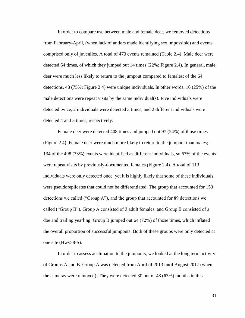
In order to compare use between male and female deer, we removed detections
from February-April, (when lack of antlers made identifying sex impossible) and events
comprised only of juveniles. A total of 473 events remained (Table 2.4). Male deer were
detected 64 times, of which they jumped out 14 times (22%; Figure 2.4). In general, male
deer were much less likely to return to the jumpout compared to females; of the 64
detections, 48 (75%; Figure 2.4) were unique individuals. In other words, 16 (25%) of the
male detections were repeat visits by the same individual(s). Five individuals were
detected twice, 2 individuals were detected 3 times, and 2 different individuals were
detected 4 and 5 times, respectively.
Female deer were detected 408 times and jumped out 97 (24%) of those times
(Figure 2.4). Female deer were much more likely to return to the jumpout than males;
134 of the 408 (33%) events were identified as different individuals, so 67% of the events
were repeat visits by previously-documented females (Figure 2.4). A total of 113
individuals were only detected once, yet it is highly likely that some of these individuals
were pseudoreplicates that could not be differentiated. The group that accounted for 153
detections we called (“Group A”), and the group that accounted for 89 detections we
called (“Group B”). Group A consisted of 3 adult females, and Group B consisted of a
doe and trailing yearling. Group B jumped out 64 (72%) of those times, which inflated
the overall proportion of successful jumpouts. Both of these groups were only detected at
one site (Hwy58-S).
In order to assess acclimation to the jumpouts, we looked at the long term activity
of Groups A and B. Group A was detected from April of 2013 until August 2017 (when
the cameras were removed). They were detected 30 out of 48 (63%) months in this

32
period, and their activity was highest in the winter months (December-February). Within
the 30 months Group A was detected, they were detected an average of 4.4 times per
month (SE 1.79), with a maximum of 25 detections in a single month. Group A did not
jump out for the first 107 times they were detected on the ramp then finally did so in
April 2016, 36 months after their first visit. They then visited the ramp 12 times without
jumping out, then jumped out again in November 2016. After that, they jumped out in 15
(47%) of the remaining 32 times they were detected on the ramp. On average, events for
this group lasted 15 minutes, and 34% of events lasted 1-2 minutes. Nine events lasted
longer than 60 minutes, and the longest event lasted 4 hours and 33 minutes.
Group B was detected 89 times from December 2015 through March 2017. They
were detected in 8 (50%) of the 16 months in this period, and their activity was
concentrated in early 2016. Within the 8 months Group B was detected, they were
detected an average of 11.1 times (SE 3.33) per month, with a maximum of 32 detections
in one month (January 2016). During this month, Group B returned to the jumpout nearly
every day, and sometimes multiple times per day. They did not jump out the first 2 times
they were detected on the ramp (in December 2015), but then proceeded to jump out the
next 3 events. These first 5 events contained only the doe, then its fawn appeared in the
6th detection. The pair did not jump out the first time they were detected together at the
jumpout, but then proceeded to jump out together for the following 7 events. Of the
remaining 76 detections, they jumped out 52 times (68%), but there was no clear pattern
across time. Additionally, sometimes this group would loiter at the top of the ramp for an
extended amount of time during a single detection event (Figure 2.5). On average, this
group stayed on and near the top of the jumpout ramp for 13 minutes, and 63% of events

33
lasted 1 minute or less. Four events lasted more than 1 hour, and the longest was 7 hours
and 11 minutes.
Four other groups of females and fawns were detected between 10 and 30 times
each (Groups C-F, Table 2.5), totaling 75 events. These groups never jumped out. There
were 4 other groups of deer that contained at least one buck (Groups G-I, Table 2.5),
which accounted for a total of 15 events. Three of these groups consisted of a single buck
and a single female, and 1 “group” was a solitary buck. In contrast to the 4 female
groups, 2 of these “with buck” groups jumped out on their 3rd visit to the jumpout (Table
2.5).
Juvenile deer were present in 142 (24%) of the 591 events that began on the ramp,
and they jumped out 47 times (33%). However, 43 (91%) of the 47 times a juvenile was
detected jumping out can be attributed to Group B (consisting of a doe and one trailing
juvenile).
DISCUSSION
Jumpouts are a promising advance in reducing WVCs, but remain relatively
untested. To our knowledge, our study is the first to monitor long enough to document
acclimation over multiple years (Clevenger and Huijser 2011), the first to account for
pseudoreplication, and the first to explore how intraspecific differences may influence
jumpout use.
Compared to deer, there were a handful of bear detections and no mountain lion
detections. Mountain lion and bear were certainly less abundant than deer in our area, but
we have detected them at other locations nearby (see Perrine 2015 for more details). We

34
have evidence that bear and mountain were crossing electrified wildlife guards (“electro-
mats”) near 2 of the jumpouts, and on 2 occasions bear were subsequently detected at the
jumpout (Perrine 2015). Deer usually travel parallel to roads before attempting to cross
(Puglisi 1974), while bear and mountain lion may try to cross sooner, thus limiting their
chances of encountering a jumpout. Likewise, deer may feel more comfortable closer to
the highway than mountain lion and bear (Rytwinski unpublished), and further, we have
evidence that carnivores may use some undercrossings more than deer (Perrine 2015),
and therefore be less likely to cross the highway itself.
The height of the jumpout is probably the primary factor in determining the jump
out rate, as well as how often the jumpout is reversed. The jumpout wall must be high
enough to discourage wildlife from jumping over the wall and entering the highway
corridor. Despite 4 reversals by mesocarnivores, we never detected a deer reversal in 299
detections below the ramp on the non-highway side of the fence. This number probably
underestimates deer activity at the base of the ramp because our cameras were aimed at
the top of the ramp rather than the base. To our knowledge, only 2 other studies have
reported ungulates reversing jumpouts, and their jumpouts were different heights from
ours. In Arizona, desert bighorn sheep reversed 1.83m jumpouts in 44 (3%) of 1312
detections on the outside of the fence; the reversals stopped after horizontal bars were
added at the appropriate height above the top of the wall (Gagnon et al. 2013). In
Colorado, there were 27 (0.9%) mule deer reversals out of 2,965 visits to their 11
jumpouts from 2012-2014 (Siemers et al. 2015). The jumpouts in Colorado varied in
height between 1.4m and 2m, and some had horizontal bars which raised their effective
height from 1.8m to 2m. The bars were installed about 0.5m above the jumpout wall, and

35
were intended to raise the effective height of the jumpout from perspective of the non-
highway side without hindering animals from jumping out (Jeremy Siemers pers.
comm.). The Arizona Department of Transportation (2013) recommends a height of 1.7 -
1.8m, and Huijser et al. (2015) suggest jumpouts 1.5m - 2.1m high appear to function
best for mule deer, elk, and bighorn sheep. The jumpouts in our study were 2m, which
was clearly high enough to discourage use to enter the highway corridor, yet perhaps too
high to encourage jumping out by a majority of individuals. Ideal height may very well
be species dependent, as different species have different jumping and climbing
capabilities.
In addition to its height, the texture (e.g., ease of purchase) of the jumpout wall is
relevant for species that can climb (Clevenger and Huijser 2011). The walls of our
jumpouts were made of plastic polymer planks buttressed by metal fence posts, which
provided minimal purchase for climbing species. Additionally, when our jumpouts were
first constructed they had a wooden plank that created a lip at the top of the jumpout wall
to discourage animals from climbing or jumping in. However, this plank was removed in
2015 after we obtained photo sequences that suggested that the flexion of the board may
have deterred deer from standing on it to jump out. We cannot conclusively determine
whether removing the plank had any effect on the jumpout rate because it is confounded
by pseudoreplication.
If the wildlife exclusion fence had worked perfectly, there would have been no
deer detected on top of any of the jumpout ramps. We did not expect this, and indeed,
deer did enter the highway corridor somehow and accessed all 4 jumpouts. Not
accounting for pseudoreplication, deer jumped out about 20% of the time. This is a

36
similar to a study in Canada that documented successful “escapes” by deer (19%), elk
(67%), and coyote (25%), however, there were only 33 total detections across these 3
species (Clevenger et al. 2002). Subsequent studies have reported higher rates of jumping
out. For example, in Arizona, bighorn sheep jumped out using 1.83m jumpouts 95% (322
of 337 events) of the time (Gagnon et al. 2013), and in Colorado, mule deer jumped out
51.5% (1333/2588) of the time using 1.3-2m jumpouts during a 2 year study (Siemers et
al. 2015). The wide variation in jumpout height for the Siemers et al. (2015) study was
due in part to the addition of horizontal bars which raised the effective height of the
jumpout. Further, there appear to be differences between the 2 deer species in the U.S.: a
study in Montana found that mule deer were 17 times more likely to jump out than white-
tailed deer (Huijser et al 2013). However, these studies did not account for
pseudoreplication, which could have potentially inflated the ratio of successful escapes in
those studies.
Ideally, we would have liked to explore relationships between successful jumpout
use and characteristics of the jumpouts. Unfortunately, this was impossible given our
sample size of 4 jumpouts. A study in Colorado with 11 jumpouts was able to quantify
some relationships, and suggested that the presence of a guide fence, shrubs closer to (but
not in) the landing area, and proximity to the highway all positively affected jumpout
success (Siemers et al. 2015). Location and spacing of jumpouts may be just as important
as characteristics of the jumpouts themselves. The Arizona Department of Transportation
(2013) recommended a jumpout every 0.8km on both sides of the road, while others have
recommended one every 0.4km (Huijser et al. 2015). Our jumpouts were ~3.2km apart on
one side of the highway and ~1.6km apart on the other side. There may be no universal

37
ideal spacing between jumpouts, but placement may be most effective in areas where
animals are most likely to enter the road corridor (i.e., near fence ends and access roads).
Group dynamics
If the same individuals return to the same jumpout multiple times, those events
are not independent, but instead pseudoreplicates. We identified at least 386 (66%) of the
584 deer detection events as individuals or groups that returned to the same jumpout
more than once. In fact, just two groups of deer (totaling 5 individuals) accounted for
47% of the deer detections over 5 years. This phenomenon is not unique to this project: in
Georgia, a single individual white-tailed deer accounted for >50% of 1,400 highway
crossings recorded in one year (Stickles et al. 2015).
Group A consisted of three female deer. This group was not always together; a
single deer identified by a unique ear notch pattern was detected more often than the
other two, but they were all detected together frequently enough to warrant grouping. In
comparison, Group B (more details below), was detected less frequently yet over a period
of time that was three times as long (51 vs. 16 months). Group A in particular appeared to
“learn” to use the jumpout. They were detected at the jumpout 107 times in 3 years
before jumping out for the first time. During the last 10 months of the study, they jumped
out 15 (47%) of 32 times suggesting that they had grown somewhat comfortable with this
behavior.
Group B consisted of a doe and yearling pair that would return to the same
jumpout day after day. Apparently, the jumpout became a part of their daily movement
patterns. This pair foraged at the top of the jumpout, and even bedded down at times. In
contrast to Group A, this pair jumped out more often and jumped out for the first time in

38
the first few visits to the jumpout. It’s possible they felt threatened during the first jump
outs, then learned that they could safely jump out after that. A more likely explanation is
that once the doe learned that jumping out was safe, her fawn simply followed suit. The
raised ramp provided food, visibility in all directions, and the option to return down the
ramp or jump out depending on where the deer might feel threatened.
We answered the question of whether deer used the jumpouts rather quickly; after
the first week of monitoring we obtained photo sequences of a deer using one of the
jumpouts to escape the highway corridor. Using Groups A and B, we were able to
explore long term acclimation to the jumpout that these groups used. Interestingly, these
two groups’ long term patterns were quite different: Group A appeared to learn to use the
jump out, while Group B starting jumping out relatively soon after their initial detection.
Monitoring for 5 years gave us previously unknown insight into how resident deer use
jumpouts over an extended time, since large mammals can take 5-6 years to acclimate to
new highway infrastructure (Clevenger and Huijser 2011).
Deer behavior
Deer in our area are most likely non-migratory, staying in the same general
vicinity while taking advantage of different microclimates within their home range
(Taber and Dasmann 1958). Further, deer home ranges tend to be relatively small; studies
on other subspecies of Mule deer have found that they range from 0.5 – 3 km2, with
males having larger home ranges than females (Harestad and Bunnel 1979). In general
mule deer are habitual animals, which includes their daily activity patterns (Chapman and
Feldhamer 1982). This probably explains why Group B would return to the jumpout day
after day: they incorporated it into their daily activity pattern. Further, there can be

39
significant variation in behavior between individual deer (Chapman and Feldhamer
1982), which is potentially why some groups would return to the jumpout over and over
and others were only detected once.
Except for during the mating season, male and female deer are generally
segregated from each other (Main and Coblentz 1990). The leading hypothesis is that this
is primarily due to sex-specific strategies to maximize fitness. In Oregon, female mule
deer tended to use areas with low coyote activity, security benefits, palatable browse
resources, and proximity to water, whereas males used areas that optimized foraging
opportunities (more biomass and species richness of forbes; Main and Coblentz 1996).
The factors that are associated with female space use are all likely to maximize offspring
survival. Roads can have a stronger negative effect on predators than their prey species,
which may be a factor in why small mammal population density can be positively
associated with roads (Rytwinski unpublished), and possibly why female deer (and their
fawns) were detected more frequently at the jumpouts in our study.
Management Implications
Jumpouts have been shown to be effective escape opportunities for large
mammals. Based on our data in the context of previous research, we recommend a
jumpout height lower than 2m, but probably not lower than 1.75m for mule deer (similar
to Huijser et al. 2015), yet the ideal height might very well be different for other species.
Jumpouts slightly lower than 2m may increase jumpout rate while still discouraging
animals from jumping in. The addition of horizontal bars seems to decrease how many
animals reverse the jumpout, while still allowing them to jump out safely, (Gagnon et al.
2013) but more research is needed into what factors contribute to successful jump outs.

40
Jumpout use by one group of deer suggests that they may acclimate to the jumpouts over
time. A necessary step is to radio collar individual animals to quantify habitat selection
and determine how animals are using the landscape near and around the highway so that
jumpout placement could be optimized. This true for deer, as well as mountain lion and
bear, especially given the amount of individual variation in behavior in deer we have
described above.

41
Table 2.1: Camera performance across all 4 sites. “Day active only” indicates that the
camera was not functional at night due to flash failure.
Site Total Survey Nights Active Not active Day active only
Hwy58-N 1840 1840 0 0
Hwy58-S 1840 1698 25 117
Wat-Dist 1840 1779 61 0
TjCk-N 1841 1815 26 0
Total 7361 7132 112 117

42
Table 2.2: The number (%) of detection events per species by site. These numbers are
irrespective of group size.
Species TjCk-N Hwy58-N Hwy58-S Wat-Dist Total
Bobcat 1 (16%) 0 4 (67%) 1 (16%) 6
Bear 2 (40%) 1 (20%) 0 2 (40%) 5
Coyote 1 (16%) 1 (16%) 4 (67%) 0 6
Mule deer 102 (11%) 157 (18%) 573 (64%) 83 (9%) 887
Grey fox 38 (67%) 0 15 (26%) 4 (7%) 57
House cat 3 (68%) 1 (16%) 0 1 (16%) 5
Opossum 2 (29%) 0 2 (29%) 3 (43%) 7
Raccoon 7 (58%) 1 (8%) 1 (8%) 3 (25%) 12
Red fox 2 (100%) 0 0 0 2
Skunk 0 0 2 (100%) 0 2
Turkey 0 3 (38%) 5 (62%) 0 8
? - Unidentifiable 0 14 (93%) 1 (7%) 0 15
Total 158 178 607 97 1007

43
Table 2.3: Number (%) of deer detection events by site. 4 different outcomes relative to
the wildlife exclusion fence: II means approached from inside and stayed inside (did not
jump out), IO means approached from inside and went outside (jumped out), OO means
approached the jumpout from outside and stayed outside, I? means the event started on
the inside (on top of the jumpout ramp) but the outcome was ambiguous, and OI means
approached the jumpout from outside and jumped in.
Site
Number of
Deer Detection
Events
Outcome
II IO OO I? OI
Hwy 58-N 157 33 (21%) 6 (4%) 118 (75%) 0 0
Hwy 58-S 553 410 (74%) 109 (20%) 29 (5%) 5 (1%) 0
Wat-Dist 83 6 (7%) 2 (2%) 75 (90%) 0 0
TjCk-N 102 23 (23%) 2 (2%) 77 (75%) 0 0
Total 895 472 (53%) 119 (13%) 299 (33%) 5 (1%) 0

44
Table 2.4: Outcomes of events that began at the top of the jumpout ramp for male and
female deer. II means approached from inside and stayed inside (did not jump out), and
IO means approached from inside and went outside (jumped out). Detections during the
months of February, March, and April were removed.
Female Male
Site Total II IO II IO
Hwy58-N 36 17 (47%) 1 (3%) 14 (39%) 4 (11%)
Hwy58-S
447
312 (70%)
101 (23%)
28 (6%)
6 (13%)
Wat-Dist
8
1 (13%)
0
5 (63%)
2 (24%)
TjCk-N
19
14 (74%)
0
3 (16%)
2 (11%)

45
Table 2.5: Initial outcomes and jumpout ratios of 10 groups of deer detected multiple
times. Groups A-F are composed of females and juveniles that were detected at least 10
times, groups G-J have a male deer in the group and were detected multiple times. IO
indicates events where the group successfully jumped out.
Group Detections IO IO%
First
Event
Events
until IO Composition
A 153 17 11 II 107 3 adult females
B 89 64 72 II 2 Doe and trailing yearling
C 28 0 0 II Never 2 adult females
D 24 0 0 II Never 2 adult females and 1 fawn
E 12 0 0 II Never 3 adult females
F 11 0 0 II Never 2 spotted fawns
G 5 0 0 II Never Buck and female
H 4 1 25 II 2 Buck and female
I 3 0 0 II Never Buck and female
J 3 1 33 II 2 Buck

46
Figure 2.1: Jumpout ramp along Highway 101 in San Luis Obispo County, California
(TjCk-N site).

47
Figure 2.2: Four jumpouts along Highway 101 between San Luis Obispo and Atascadero,
California. The wildlife exclusion fence is 4 km long.

48
Figure 2.3: Deer activity at all 4 jumpouts irrespective of group size.

49
Figure 2.4: Comparison of male and female deer with the months of February-April
removed. Total detections only includes events that started at the top of the ramp. Red
bars indicate how many groups/individuals jumped out, and green bars indicate how
many detections were unique groups/individuals.

50
Figure 2.5: Male deer about to jump out at the Hwy58-S site.

51
Figure 2.6: A doe and yearling fawn pair (Group B) bedded down the Hwy58-S jumpout.

52
CHAPTER 3
WILDLIFE USE OF UNDERCROSSINGS ALONG A HIGHWAY WITH
WILDLIFE EXCLUSION FENCING
INTRODUCTION
Roads have significant ecological impacts, including direct and indirect effects
upon wildlife populations and habitat structure (Forman and Alexander 1998). Wildlife-
vehicle collisions (hereafter WVCs) and the associated injuries and deaths to both wild
animals and humans are the most apparent effects. It has been estimated that 1,000,000
vertebrates are killed on United States roads every day (Forman and Alexander 1998).
The majority of these deaths are small, r-selected taxa like rodents and songbirds, which
can reproduce faster than the rate they are killed by vehicles. However, for species that
are less abundant (often large bodied and k-selected taxa), WVCs can be a significant
population-level mortality factor. For example, 50% of Florida panther (Puma concolor
coryi) mortality, and a significant proportion of Key white-tailed deer (Odocoileus
virginianus clavium) mortality was attributed to WVCs before safe crossing opportunities
were constructed (Forman and Alexander 1998). WVCs involving large-bodied mammals
such as deer (Odocoileus sp.) also affect human safety; every year in the United States
deer-vehicle collisions cause >29,000 injuries (about 80 per day), 150-200 human deaths,
and damages averaging >$6,600 per collision (Mastro et al. 2008, Huijser et al. 2009,
Stull et al. 2011).
In addition to direct mortality, roads can be significant barriers (Poessel et al.
2014) or filters (Clevenger and Waltho 2005) to the movement of wildlife. Forman
(2000) estimated that 15-20% of U.S. land is ecologically affected by roads. Animals

53
may not only hesitate to cross roads when encountered, but actively avoid them as well.
Further, large mammals (especially carnivores) are vulnerable to habitat fragmentation
because of their relatively large home ranges, lower population densities, and conflicts
with humans (Crooks 2002). For example, in the Southwest U.S., mountain lion (Puma
concolor) home ranges tended to be in areas with relatively lower densities of improved
dirt and paved roads (Van Dyke et al. 1986). Similarly, in the Netherlands, high road
density was explicitly linked to European badger (Meles meles) population declines,
which was attributed to avoidance of disturbed habitat as well as vehicle mortality (Van
der Zee et al. 1992).
Various mitigation measures have been used to modify animal behavior to reduce
WVCs. Wildlife exclusion fencing has been found to be the most effective (non-lethal
control) method for reducing collisions with deer (Clevenger and Huijser 2011). Despite
reducing WVCs, wildlife fencing may further decrease a road’s permeability for wildlife;
therefore, it is suggested that fencing be designed to funnel animals towards crossing
structures (Huijser at al. 2015). In some areas, well designed, implemented, and
maintained wildlife exclusion fencing combined with wildlife crossings has resulted in an
80-100% reduction in WVCs involving large mammals (Huijser et al. 2015).
Wildlife overcrossings and undercrossings have become the standard methods to
increase road permeability. When compared to undercrossings, overcrossings seem to be
used by a broader suite of species, although they are less common probably due to being
more expensive to build (Clevenger and Waltho 1999, Van Wieren and Worm 2001). We
categorize undercrossings into two categories: culverts and underpasses. Culverts are
usually originally designed to carry water under roads, although they can be retrofitted or

54
even built for the purpose of wildlife use. They can vary in size and composition from
0.3m corrugated pipes to 4mx4m concrete box culverts. In contrast, underpasses are often
taller, and much wider than culverts, providing much more open passage for wildlife.
Further, underpasses are often built over natural substrate (as opposed to culverts which
are often concrete or metal), which probably further facilitates wildlife use. As with the
overcrossings, underpasses tend to accommodate a wider suite of species than culverts
(Glista et al. 2009).
Our objective was to determine which factors are related to use of undercrossings
by mule deer (Odocoileus hemonius californicus), black bear (Ursus americanus),
mountain lion (Puma concolor), and bobcat (Lynx rufus). We chose deer as a focal
species because a combination of their large size and abundance make them a significant
safety concern for drivers. Mountain lion and bear are also a concern from a human
safety standpoint, and regional connectivity is important for these wide-ranging species.
Bobcats were a focal species because they can be an ecological indicator species for
habitat fragmentation in California (Jennings 2013) by providing insight into connectivity
on a sub-regional scale, and are representative of the mesocarnivore guild, which plays
important ecological roles such as mediating trophic cascades (Roemer et al. 2009).
Many studies have documented wildlife use of undercrossings, but far fewer have
attempted to correlate use with features of the undercrossings. Several studies have found
that deer use larger and more open undercrossings (Mastro et al. 2008, Clevenger and
Waltho 2005), and we expected to find these same patterns in our study area (see below).
However, despite decades of research, it is still unclear which factors are associated with
use by carnivores in particular. Some studies have found that large carnivores used

55
smaller and longer undercrossings more than larger and shorter ones(e.g., Clevenger and
Waltho 2005), but the associations were not as consistent as for deer. We expected
mountain lion and bear to use smaller culverts more than larger ones, and surrounding
habitat to have an effect on use. We expected bobcats to use smaller culverts more than
larger culverts.
Most wildlife crossing monitoring projects may not be long enough to account for
yearly variation and wildlife acclimation. The average monitoring duration of wildlife
crossing projects is 17 months, while some species can take 5-6 to adapt to new
infrastructure in their enviroment (Clevenger and Huijser 2011). We monitored most of
our undercrossings for more than 4 years, and all but one for 2 years or more, which
allowed us to account for yearly variation as well as long term acclimation to wildlife
exclusion fencing.
METHODS
Study site
Our study was along a 19.3 km section of U.S. Highway 101 in San Luis Obispo
County, California (latitude 35.365, longitude -120.638), between the cities of San Luis
Obispo and Atascadero (Figure 3.1). In this region, Highway 101 is a major regional
transportation corridor, with traffic volume of to 4,000 vehicles per hour (Snyder 2014).
Just north of San Luis Obispo, the highway passes through the Santa Lucia mountains,
which is part of a relatively narrow band of the Los Padres National Forest. The
surrounding landscape is representative of the California Woodland Chaparral Ecoregion,
which is characterized by oak woodland and chaparral communities, interspersed with
56
annual and perennial grasslands, and some riparian habitat (deVos et al. 2003). Here, the
oak woodland habitat is composed of Coast live oak (Quercus agrifolia), Poison oak
(Toxicodendron diversilobum), Toyon (Heteromeles arbutifolia), Ceanothus spp. (e.g.,
California lilac), and Artostaphylos (Manzanitas and Bearberries; Barbour et al. 2007).
The dominant species in the Chaparral habitat are California Sage (Artemisia
californica), Black Sage (Salvia mellifera), Coyote Bush (Baccharis pilularis), and
Mountain Mahogany (Cercocarpus spp.; Barbour et al. 2007). The region’s climate is
“Mediterranean”, with hot dry summers, mild wet winters, and considerable annual
variation in precipitation (Sommer 2007).
Computer modeling has identified this area as an important regional and local
movement corridor for mountain lion, mule deer and black bear (Thorne et al. 2006,
Thorne and Huber 2011), and field surveys have indicated that this area is a hotspot for
roadkills of these taxa (Siepel et al. 2013, Shilling and Waetjen 2015). In particular, the
roadkills were concentrated in a 4km section of the highway where the surrounding
habitat was relatively forested, and the computer models indicated higher levels of
landscape connectivity for our focal species. To minimize large-mammal roadkills and
protect human safety in this area, the California Department of Transportation (hereafter
CalTrans) constructed a 4 km wildlife exclusion fence along the roadkill hotspot that was
completed in April 2012 (Siepel et al. 2013; Figure 3.1).
Data collection
There were dozens of undercrossings along Highway 101 within and adjacent to
the wildlife exclusion fence zone. Since our focal species were medium to large sized
mammals we chose to document activity in only those with a width and height ≥1.2 m (4
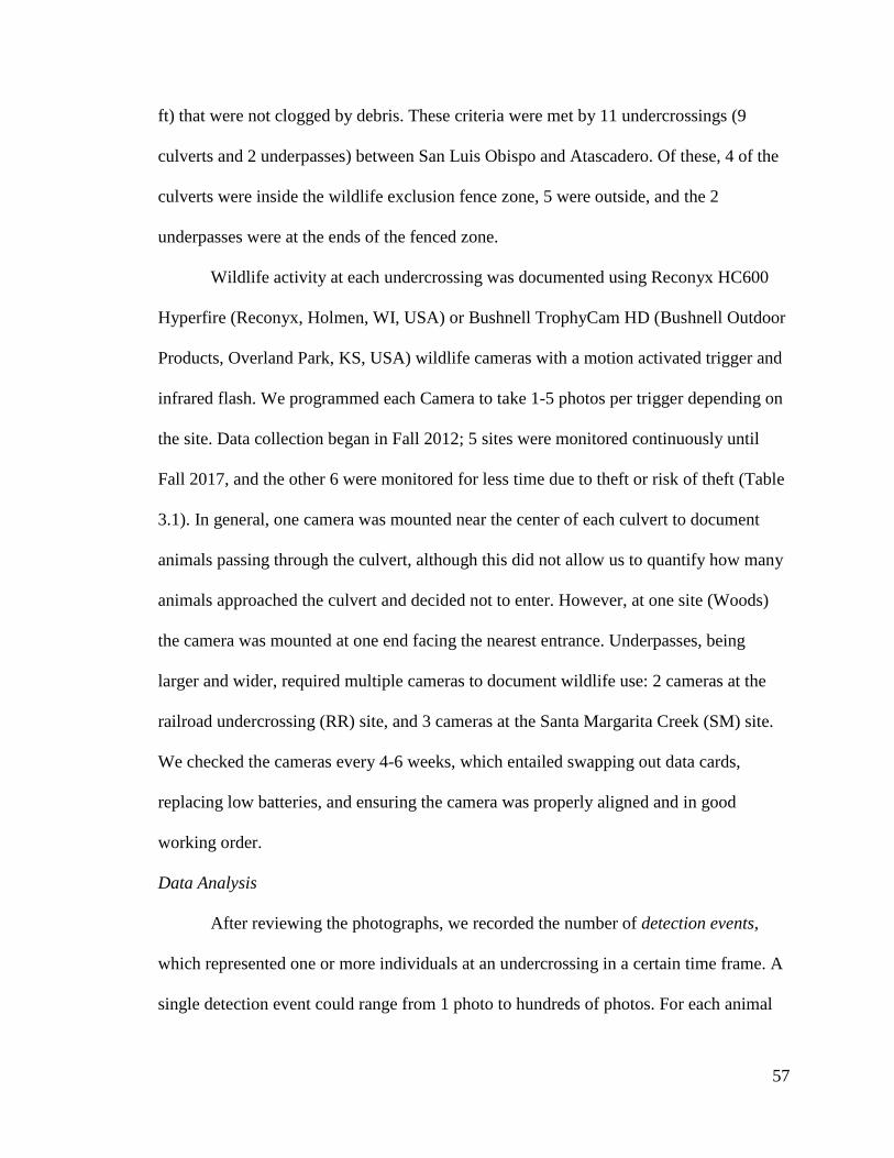
57
ft) that were not clogged by debris. These criteria were met by 11 undercrossings (9
culverts and 2 underpasses) between San Luis Obispo and Atascadero. Of these, 4 of the
culverts were inside the wildlife exclusion fence zone, 5 were outside, and the 2
underpasses were at the ends of the fenced zone.
Wildlife activity at each undercrossing was documented using Reconyx HC600
Hyperfire (Reconyx, Holmen, WI, USA) or Bushnell TrophyCam HD (Bushnell Outdoor
Products, Overland Park, KS, USA) wildlife cameras with a motion activated trigger and
infrared flash. We programmed each Camera to take 1-5 photos per trigger depending on
the site. Data collection began in Fall 2012; 5 sites were monitored continuously until
Fall 2017, and the other 6 were monitored for less time due to theft or risk of theft (Table
3.1). In general, one camera was mounted near the center of each culvert to document
animals passing through the culvert, although this did not allow us to quantify how many
animals approached the culvert and decided not to enter. However, at one site (Woods)
the camera was mounted at one end facing the nearest entrance. Underpasses, being
larger and wider, required multiple cameras to document wildlife use: 2 cameras at the
railroad undercrossing (RR) site, and 3 cameras at the Santa Margarita Creek (SM) site.
We checked the cameras every 4-6 weeks, which entailed swapping out data cards,
replacing low batteries, and ensuring the camera was properly aligned and in good
working order.
Data Analysis
After reviewing the photographs, we recorded the number of detection events,
which represented one or more individuals at an undercrossing in a certain time frame. A
single detection event could range from 1 photo to hundreds of photos. For each animal
58
detection event at a site, we documented the date, start time and end time, species,
number of individuals, and age class (adult or juvenile). For deer we also noted whether
each individual had visible antlers or not. We counted animals of the same species
traveling together as one detection event, because their activity was likely interdependent
(Allen et al. 2013). To account for potential dependence between events we set a 15-
minute buffer period before a detection of the same species at the same site was
considered a different event. We recorded each camera’s performance by month and
excluded months when the camera was active for < 10 nights. We excluded photos from
periods when the camera was inactive or otherwise malfunctioning (i.e., diurnal photos
when the camera failed to flash at night). Reasons the camera was inactive included
battery failure, full data cards, theft, and being knocked off aim.
Our dependent variable was the count of detections of a particular focal species
per site per month. We chose 9 predictor variables: YEAR, SEASON, LANDSCAPE
RESISTANCE, LENGTH, OPENNESS, DISTANCE TO COVER, SUBSTRATE,
whether the undercrossing was in the wildlife exclusion FENCE zone, and HUMAN
ACTIVITY. We used YEAR and SEASON in every model in order to account for
temporal variation among and within years. We collected data in 6 different years: 2012-
2017. SEASON had four categories: Winter (December-February), Spring (March-May),
Summer (June-August), and Fall (September-November).
We used LANDSCAPE RESISTANCE in every deer, bear, and mountain lion
model to account for the likelihood of deer, bear, and mountain lion being near the
culvert entrances in the first place. Habitat suitability can sometimes be the strongest
predictor of a particular species use of undercrossings (Yanes et al. 1995, Clevenger and

59
Waltho 2000). No matter the species, if the undercrossing is in poor habitat, it is probably
less likely to be used, and vice versa. In our case, LANDSCAPE RESISTANCE was
modeled based on vegetative community, road density, and topography (Thorne and
Huber 2011). We expected a higher value of LANDSCAPE RESISTANCE to indicate
lower activity of a given focal species in that area. We followed the same assumption as
Clevenger and Waltho (2000); namely, that each individual is aware of every
undercrossing and can choose based on attributes alone. We used ArcMAP 10 (ESRI,
Redlands, CA, USA) to create a 500m (same distance as Grilo et al. 2008) habitat buffer
zone around each culvert center. We then split each circle in half using the “split
polygons” tool with a Highway 101 layer (CalTrans California Highways) buffered by 20
meters to account for the right of way. We received landscape resistance surfaces for
mountain lion, deer, and bear from Thorne and Huber (2011), and used the “Zonal
Statistics” tool to find the average resistance value within each buffer zone (Table 3.2b).
We chose the higher of the 2 resistance values for each undercrossing to be conservative,
assuming that the higher value would be the most biologically relevant. Two culverts
(58N and 58S) were in series with a 20m uncovered drainage between them, so for these
sites, we used the polygon on the east side of the highway for the culvert under the
northbound lanes, and the polygon on the west side of the highway for the culvert closer
to the southbound lanes. A resistance surface was not made by Thorne and Huber (2011)
for bobcats because they are not a species of concern from a highway safety standpoint
and landscape-level connectivity is not as important for bobcats as it is for our other focal
species (Crooks 2002, Jennings and Lewison 2013).

60
Undercrossing dimensionality has been shown to be an important predictor of
wildlife activity (Clevenger and Waltho 1999, Mastro et al. 2008). We quantified
undercrossing dimensionality by measuring the length, width, and height of each
undercrossing (Table 3.2a). At two culverts the height was slightly different at each
entrance so we averaged the two values. For the two underpasses we used Google Earth
Pro (Google Inc. Mountain View, CA USA) to measure length and width, and used a tape
measure to measure the height. Even though the highway was divided above each
underpass we included the section between the northbound and southbound lanes in the
length measurement. We used these values to calculate “openness” (Reed and Ward
1985), an index combining height, width, and length into a single value:
Openness = (ℎ𝑒𝑖𝑔ℎ𝑡 × 𝑤𝑖𝑑𝑡ℎ) ÷ 𝑙𝑒𝑛𝑔𝑡ℎ
We also measured the shortest distance to cover from each culvert entrance, and
averaged those two values for each site (Table 3.2a). We defined cover as any vegetation
that was at least 1m high and was dense enough to reasonably shelter a medium sized
animal (like a bobcat). At 1 culvert (N 10.0), there was no cover within 100m of either
entrance, and both underpasses were too wide to have an “entrance”; for these cases, we
set the DISTANCE TO COVER to twice the longest distance to cover measured at any
other site. For SUBSTRATE, we recorded the predominant substrate type in each
undercrossing, as either concrete or natural sediment (Table 3.2b). Location relative to
the wildlife exclusion fence refers to whether or not the undercrossing was located
between the two ends of the wildlife exclusion fence (Table 3.2b). Human activity was
quantified in nearly the same way as our focal species (Table 3.2b). Because it was much
easier to differentiate humans from each other, we used a 6-hour buffer before identifying
61
the same individual as a new event. We did not include members of our field team
checking the cameras because this was consistent across all sites. We also recorded
whether the culvert’s exit could be seen from its entrance, but decided to remove it from
the analysis because only one culvert was not see through.
We built zero-inflated Poisson regression models (Lambert 1994) to determine
which factors were associated with undercrossing use by our focal species. YEAR,
SEASON, and LANDSCAPE RESISTANCE were included in all deer, bear, and
mountain lion models. An example model for deer would be YEAR, SEASON,
LANDSCAPE RESISTANCE, LENGTH with underpass length being the variable of
interest in this case. YEAR and SEASON were included in all bobcat models, so an
example model would be YEAR, SEASON, LENGTH with length as the variable of
interest. We considered standardizing each month using active nights to control for
variation in survey effort, but this variance was so minimal (75% of months had 30
survey days, 90% of months had 28 survey days), that we decided this was not necessary.
We fit zero-inflated Poisson regressions on the count of each of our focal species with the
following factors as predictors: LANDSCAPE RESISTANCE, LENGTH, OPENNESS,
AVERAGE DISTANCE TO COVER, SUBSTRATE, LOCATION RELATIVE TO
FENCE, and HUMAN ACTIVITY. We used a zero-inflated Poisson model because our
data were count-based and we had a significant number of months where we did not
detect a particular focal species.
With the exception of deer, we ran each of our models twice, once with all
undercrossings included and the second time after removing the underpasses. The
underpasses were removed in the 2nd suite of models because they were so fundamentally

62
different in structure and dimensionality than the culverts. For deer, we only ran models
with underpasses included because deer were almost solely detected at those two
locations (95.7% of detections). Significance was determined at the 0.05 level, and all
data analysis was completed in JMP 13 (SAS Institute Inc., Cary, NC, USA).
RESULTS
Across our 11 sites, the cameras were active a total of exactly 15,000 survey
nights. There was variance in survey effort due to battery failure, theft, or fear of theft of
our cameras (Table 3.1). At the maximum, several sites were monitored continuously
during our 5-year study period (~1800 nights), and at the minimum one site was
monitored for only 7 months (207 nights; Santa Margarita Creek underpass) due to theft.
Across all 11 sites, we acquired 2,015 detections of our four focal species. Bobcat were
most frequently detected (n=1,231), followed by deer (n=610), then bear (n=142) and
mountain lion (n=32).
Mountain lion were detected at 6 of 11 sites, with one site (N3.1) accounting for
46.9% (15/32) of all detections (Table 3.5a). Bear were detected at 8 sites (Table 3.5b),
and most sites averaged 1 bear detection every 1-3 months. Deer were also detected at 8
sites (Table 3.5b), with 95% (581/610) of deer detections occurring at the two
underpasses, where they were detected once every 1-2 days on average. Deer were
detected at 5 of the culverts <5 times each despite them being monitored for longer than
the underpasses. Bobcats were detected at every site, but with considerable variation in
activity between sites, ranging from only 2 detections in 4 years of monitoring (at 58N),
to averaging 9 visits per month (at N3.1; Table 3.5a).

63
Landscape resistance
In the models with all undercrossings included, there was no evidence for an
effect of LANDSCAPE RESISTANCE on mountain lion (p=0.411), or deer (p=0.3026)
activity, yet LANDSCAPE RESISTANCE had a negative effect on bear activity
(p=0.0003). After removing the underpasses, there was still no evidence for an effect of
LANDSCAPE RESISTANCE on mountain lion activity (p=0.250), and the negative
effect on bear activity remained (p=0.0006).
Dimensionality
To avoid collinearity in our model, we removed HEIGHT and WIDTH from the
analysis because they were significantly (>0.7) correlated with OPENNESS (Figure 3.2).
The all-undercrossings models indicated no evidence for an effect of OPENNESS on
mountain lion activity (p=0.270) or bear activity (p=0.062), but OPENNESS was
positively related to deer activity (p<0.0001) and negatively related to bobcat activity
(p<0.0001). In the culvert-only models, there was still no evidence for an effect of
OPENNESS on mountain lion activity (p=0.176) or bear activity (p=0.124), and a
positive effect on bobcat activity (p<0.0001). In the models with all undercrossings
included there was no evidence for an effect of LENGTH on mountain lion activity
(p=0.726) or bear activity (p=0.091), a negative effect on deer activity (p<0.0001), and a
positive effect on bobcat activity (p=0.0027). In the culvert only models, LENGTH had a
positive effect on mountain lion activity (p=0.005), and no evidence for an effect on bear
(p=0.485) or bobcat (p=0.443) activity.
64
Distance to cover and substrate
The all-undercrossings models indicated no evidence for an effect of DISTANCE
TO COVER on mountain lion activity (p=0.263) or bear activity (p=0.887), a positive
effect on deer activity (p<0.0001), and a negative effect on bobcat activity (p<0.0001). In
the culvert only models, there was still no evidence of an effect of DISTANCE TO
COVER on mountain lion activity (p=0.145) or bear activity (p=0.102), and had a
negative effect on bobcat activity (p<0.0001).
In the all-undercrossings model, mountain lion (p=0.015), deer (p<0.0001), and
bobcat (p<0.0001) activity was higher in undercrossings with natural substrate, while
bear activity was not associated with SUBSTRATE (p=0.186). In the culvert only
models, there was no longer evidence that SUBSTRATE was associated with mountain
lion activity (p=0.595) or bear activity (p=0.864), but bobcat activity was still higher in
undercrossings with natural substrate (p<0.0001).
Fencing and human activity
In the all-undercrossings model mountain lion (p=0.046), deer (p<0.0001), and
bobcat (p<0.0001) activity was higher outside the wildlife exclusion fence zone, while
bear activity was higher inside (p<0.0001). In the culvert-only models, there was no
longer evidence for an effect on mountain lion activity (p=0.058), but there was still
higher bear activity inside (p<0.0001), and higher bobcat activity outside (p<0.0001).
There was human activity at every site, but most sites on averaged <1 event every
2 months (Table 3.2b; Figure 3.7), while the 2 sites with the most human activity had
between 1.5 and 2 human detection events per month (N3.1 and SmCk underpass). At 2
sites (58S and 58N) we only detected one person in ~4 years of monitoring at two sites,

65
and our maximum was 60 human crossings at a site we monitored for ~3 years (N3.1). In
the all-undercrossings model, there was no evidence for an effect of HUMAN
ACTIVITY on mountain lion activity (p=0.415), bear activity (p=0.140), or bobcat
activity (p=0.719), and a positive effect on deer activity (p<0.0001). In the culvert-only
models, there was still no evidence that HUMAN ACTIVITY had an effect on mountain
lion activity (p=0.231), bear activity (p=0.130), or bobcat activity (p=0.228).
DISCUSSION
Wildlife crossings are critical for providing connectivity across highways,
especially when associated with wildlife exclusion fencing. However, the specific
characteristics associated with high wildlife use are poorly known, and probably better
understood for ungulates than for carnivores. We documented mule deer, black bear,
mountain lion, and bobcat activity at 11 undercrossings along Highway 101 near San
Luis Obispo, California for 7-61 months between 2012-17. We found significant
variation between our four focal species regarding undercrossing activity and associations
with various factors.
Deer
Although deer were detected at 8 of the 11 sites, they clearly used the underpasses
far more than the culverts. After controlling for survey effort, there was 100x more deer
activity at the 2 underpasses compared to the 9 culverts. Since our cameras were usually
located in the middle of the culverts, we were unable to determine the extent that deer
approached culverts but declined to enter. However, at one site (Woods), we mounted the
camera at the far entrance to minimize the likelihood of human disturbance, and detected

66
several events consisting of deer approaching the culvert entrance but then turning away
rather than passing through the 1.8m wide, 2.4m high concrete box culvert. Even at the
large, open, and heavily utilized Santa Margarita Creek underpass, several photo
sequences suggested that the deer were hesitant to cross under the highway, perhaps due
to the noise of vehicles that the deer could not see. This hesitant behavior when
approaching culverts has been documented by others: in Colorado, 61% of the local mule
deer population used a 3m x 3m culvert to safely cross the highway (Reed et al. 1975).
Deer are migratory in this area in Colorado (Reed et al. 1975), while in our study area the
deer are likely resident (Taber and Dasmann 1958). This difference in life history may
explain why a large proportion of deer were willing to use the culvert in the Colorado
study.
Our findings are consistent with multiple studies that have shown that deer avoid
small confined culverts. Mastro et al. (2008) quantified the effect of culvert openness on
mule deer activity and found that sites >0.8 were selected, and <0.6 was avoided. All of
our culverts had openness ratios <0.3 while the underpasses had openness ratios of
around 13 (Table 3.2a). Oddly, the culvert with the highest deer activity (n=16; Woods)
had one of the lowest openness ratios (0.1), yet this may be the same individual returning
over and over. In Canada, deer tended to use more open undercrossings (Clevenger and
Waltho 2005), and used wildlife overpasses 4-15 times more than underpasses
(Clevenger and Barrueto 2014). In an earlier study in Canada, ungulates actually selected
for smaller, less open undercrossings; yet these undercrossings were significantly less
noisy and further from human habitation than larger undercrossings, which likely
confounded the results (Clevenger and Waltho 2000).

67
The remaining significant factors (LANDSCAPE RESISTANCE, distance to
COVER, within the exclusion FENCE zone, SUBSTRATE, and HUMAN ACTIVITY)
could all be explained by the fact that deer almost exclusively used the 2 underpasses.
The two underpasses’ approaches were in areas with relatively low movement cost,
higher than average distance to cover, were at the ends of the wildlife exclusion fence,
had natural substrate, and average human use. Regarding distance to cover, mule deer in
Canada selected for undercrossings with higher distance to cover, perhaps feeling safer
with higher visibility (Clevenger and Waltho 2005).
Human activity might have an impact on deer activity, but it’s almost certainly
not as important as dimensionality. In Canada, human activity had a slight negative
impact on deer use of culverts (Clevenger and Barrueto 2014), and in Spain, ungulates
never used any passages below a railway, with human activity suggested as the primary
deterrent (Rodriguez et al. 1996). Our results indicate that both humans and deer tended
to avoid the smallest culverts, and overall, ungulates are probably less sensitive to human
activity than most carnivores.
Bear
Overall, bear were the least discriminating of our focal species. They used one of
the two underpasses and, except for the Tassajara Creek culvert, most of the remaining
undercrossings at relatively similar frequencies. We never detected a bear using the Santa
Margarita Creek underpass in 7 months of monitoring, which is interesting given than it
seems to be an important route under the highway for mountain lion, deer, and other taxa.
Bear have used this underpass in the past (Perrine and Snyder 2011), thus it is possible

68
(and maybe likely) that we would have detected bear there if we had monitored for longer
given they are moderately infrequently detected.
The only factor that was significant in both suites of models was whether the
undercrossing was inside the wildlife exclusion fence zone; bear activity was higher at
sites within the wildlife fence zone. Considering that the wildlife exclusion fence zone
was constructed in part due to 5 bears being hit during a 6 week period along a 4 km
stretch of the highway (Siepel et al. 2013), this is potentially good news. Bear using the
undercrossings in the wildlife exclusion fence zone is good from a habitat connectivity as
well as highway safety perspective; unfortunately, no quantification of wildlife use of
undercrossings occurred prior to the fence construction (Perrine 2015).
We found no evidence for an effect of length or openness on bear activity in our
models. In contrast, in Banff National Park, Canada, black bear activity was higher in
longer and less open undercrossings (Clevenger and Waltho 2005, Clevenger and
Barrueto 2014). This pattern conforms to evolved behavior and life history trait for black
bears. The longer, more constricted crossing structures black bears tend to use most (or at
least not avoid in our case) for safe passage might be explained by these species’
requirements for cover and avoidance of exposed, sparsely wooded habitats (Kansas and
Raines 1990, Lyons et al. 2003).
If bear are tolerant of undercrossing dimensionality and structure, then the most
important factor may be habitat suitability. Bear were detected only one time at any of the
3 drive-through culverts north of the wildlife exclusion fence, strongly suggesting that
these structures provide little connectivity for bear despite the size of the structures. This
is perplexing, because these culverts are larger and better-lit than some of the culverts

69
that bear used in the wildlife fence zone. It seems likely that bears cross the highway at
grade where there is no wildlife exclusion fence and no concrete median barrier, or
perhaps simply do not use this area very much. The habitat here is somewhat different
than the rest of the study area to the south, being mostly open rangeland as opposed to
denser oak woodland. However, landscape models identified the area near these drive-
through culverts as potentially high-connectivity habitat for bears (Thorne and Huber
2011). Having bear with GPS collars would give us insight into their movement and
habitat selection near the highway.
Mountain lion
Mountain lions have large home ranges and low population densities (compared to
bobcats and deer at least; Sargeant et al. 1998), so it is not surprising that there were
relatively few detections (n=32). Ng et al. (2004) detected mountain lion only once
during 1 year of monitoring 17 undercrossings along ~50km of highway in southern
California.
Despite not being detected very often, mountain lions used a variety of
undercrossing types: they were detected at both underpasses, a large corrugated pipe
culvert, and 3 concrete box culverts (Table 3.5a). One of the concrete box culverts was
only 1.2m high, while the others were 3.7m and 2.1m high. In the all-underpasses model,
there was no evidence that dimensionality had an effect on mountain lion activity.
However, in the culvert-only models, mountain lion activity was significantly higher in
longer culverts. There were no drastic differences between the lengths of the culverts
(Table 3.2a); most were between 38.1m and 53.3m long. There is relatively little
literature on mountain lion use of undercrossings. In Canada, mountain lions selected for

70
longer and narrower undercrossings (Clevenger and Waltho 2005), but a later study
found that dimensionality did not have an effect on mountain lion activity (Clevenger and
Barrueto 2014).
We expected habitat suitability to be one of the most important factors driving
mountain lion use of undercrossings. Interestingly, we found no evidence for an effect of
landscape resistance on mountain lion activity in undercrossings. In Southern California,
mountain lions selected for woody cover over more exposed habitats (Beier et al. 1995);
however, in Canada, mountain lion activity was highest at crossing structures with less
vegetative cover within a 1km radius (Clevenger and Barrueto 2014). Also in Southern
California, mountain lions were documented traveling along riparian corridors that led
into undercrossings (Beier et al. 1995). In our study, the site with the second highest
detections (Wat-Dist) is part of a small stream drainage that may have facilitated
mountain lion movement. It is also possible that some of these detections were repeat
visits by one or a few individuals.
It is slightly surprising that mountain lion activity was evidently not associated
with more cover near the entrances in either model. Mountain lions usually select
forested habitat over open habitat (Koehler and Hornocker 1991), and in Southern
California mountain lions selected for undercrossings with “ample woody cover” (Beier
et al. 1995). Human activity did not have an impact on mountain lion activity in either
model. This is not too surprising given how infrequently mountain lions were detected,
but other studies have found that mountain lions actively avoid humans. For example,
mountain lions in Northern California spent significantly less time at and were less likely
to return to carcasses after playback of human voices versus a playback of frog chorus

71
(Smith et al. 2017). In Canada, human activity had a slight negative impact on mountain
lion use of crossing structures (both over and undercrossings; Clevenger and Barrueto
2014).
Bobcat
Bobcats were the only focal species to use every undercrossing, yet activity was
higher at less open, longer undercrossings. This is consistent with Clevenger and
Waltho’s (1999) findings that most carnivores generally select less open undercrossings.
However, once we removed underpasses, bobcats selected for more open culverts. It may
be that bobcats do not like how exposed underpasses are, yet prefer culverts that are less
confined, or other factors are influencing their patterns.
Bobcats selected undercrossings with a shorter distance to cover in both models.
This is not surprising; as a mesocarnivore, bobcats generally select for the safety of cover
over exposed terrain (Rodriguez et al. 1996). Ng et al. (2004) found that suitable habitat
(within 250m) on either side of the undercrossing was positively related to use by
bobcats; thus if we define cover as suitable habitat then the results of our study support
Ng et al.’s (2004) findings. Bobcats were detected more often in undercrossings outside
our wildlife exclusion fence in both models. If bobcats are crossing the highway in our
study area on top of the road, we would expect more activity inside the fenced zone, and
less outside, because bobcats can cross the road at grade outside the fenced zone. This
either means bobcats do not cross the road at grade (not likely), or that the undercrossings
they preferred happened to be outside the fence (more likely).
Human activity did not affect bobcat use of undercrossings in either model.
Human activity and development can have negative impacts on carnivore use of

72
undercrossings (Clevenger and Waltho 2000, Ng et al. 2004), yet bobcats are probably
the most urban-adapted wild felid (Riley et al. 2010). Our undercrossings are in a
relatively rural area, and may have simply not had enough human activity to impact
bobcat undercrossing use.
Next steps
There are more questions we plan to explore with this data set. Given that human
activity is correlated with culvert dimensions (negatively with height in particular) we are
planning to examine temporal interactions between humans and wildlife. We are also
interested in mesocarnivore interactions and use of undercrossings. The majority of our
detections are mesocarnivores (particularly grey fox, bobcat, skunk, and opossum
(Didelphis virginiana)), so it may be worthwhile to examine any spatial or temporal
partitioning between these species. Putting GPS collars on mountain lion, bear, and deer
in our area is a logical next step. As of this writing (spring 2018), a mountain lion
collaring project is underway in the greater region containing our study area. GPS collar
data will reveal further insights into how mountain lions interact with the highway in our
area.
Management implications
We found that dimensionality had significant effects on deer and bobcat use of
undercrossings, but not mountain lion and bear activity. Deer prefer underpasses over
culverts, and bobcats seem to prefer larger culverts over smaller culverts but will also use
underpasses. Surrounding habitat is probably an important factor for bear and mountain
lion, and on a more local scale, for bobcat.
73
Aside from a long-term wildlife crossing project in Canada (Clevenger and
Barrueto 2014), we are the first study to document wildlife activity at undercrossing for
at least 5 years. It is important for projects to last for this long because wildlife can take
up to 4-6 years to adapt to new infrastructure (Clevenger and Huijser 2011). Our 5-year
dataset provides evidence that with crossing structures, highways are impenetrable
barriers to large and medium sized mammals. This is particularly important for mountain
lions, whose large home ranges (up to 320 square km) can be reduced by the barrier
effects of roads. Further, roads are one of the biggest sources of mortality for young male
mountain lions dispersing to new areas (Beier et al. 2005). Given the high degree of
urbanization in some parts of California, connecting the remaining quality habitat for
mountain lions (and other species with large movement needs) is critical, especially since
California mountain lions are composed of separate populations (Ernest et al. 2003).
Trophic level may have an effect on what type of crossing structures are most
effective for promoting connectivity. Top predators like mountain lions and black bears
were not influenced by dimensionality to the same extent that deer and bobcat were. We
agree with Cramer and Bissonette (2005) that bigger undercrossings are generally better,
cover is probably important at the ends of undercrossings especially for prey species, and
deer strongly select for larger underpasses while carnivores are more plastic. In fact,
underpasses may be so different structurally from culverts that we caution researchers
from pooling them in the same models in future studies. Grilo et al. (2008) suggests that
managing the surrounding habitat around undercrossings may be the most cost-effective
way to increase use by wildlife. If affordable, overcrossings probably provide the most

74
connectivity for multiple species (Clevenger and Waltho 1999, Van Wieren and Worm
2001).

75
Table 3.1: Total survey effort for each site, including monitoring time frame.
Type Site Month begin Month end Survey Nights
Culvert Woods Sep-2012 Sep-2017 1746
Culvert N3.1 Sep-2012 Oct-2015 1071
Culvert TjCk Aug-2012 Oct-2015 1163
Culvert Wat-Dist Aug-2012 Sep-2017 1866
Culvert 58N Jan-2013 Jul-2016 1301
Culvert 58S Sep-2012 Jul-2016 1422
Culvert N8.5 Aug-2012 Sep-2017 1856
Culvert N9.1 Aug-2012 Sep-2017 1849
Culvert N10.0 Aug-2012 Sep-2017 1808
Underpass RR Jul-2012 Jul-2014 711
Underpass SM Aug-2012 Mar-2013 207
Total 15,000
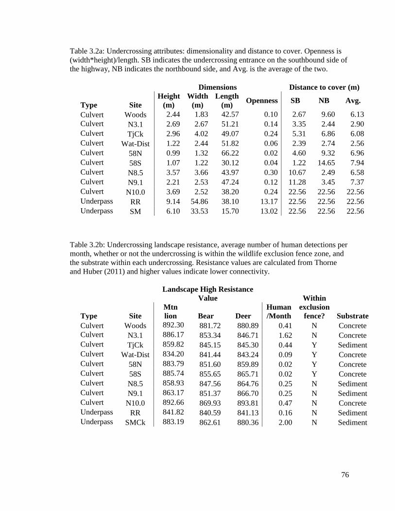
76
Table 3.2a: Undercrossing attributes: dimensionality and distance to cover. Openness is
(width*height)/length. SB indicates the undercrossing entrance on the southbound side of
the highway, NB indicates the northbound side, and Avg. is the average of the two.
Type Site
Dimensions Distance to cover (m)
Height
(m)
Width
(m)
Length
(m) Openness SB NB Avg.
Culvert Woods 2.44 1.83 42.57 0.10 2.67 9.60 6.13
Culvert N3.1 2.69 2.67 51.21 0.14 3.35 2.44 2.90
Culvert TjCk 2.96 4.02 49.07 0.24 5.31 6.86 6.08
Culvert Wat-Dist 1.22 2.44 51.82 0.06 2.39 2.74 2.56
Culvert 58N 0.99 1.32 66.22 0.02 4.60 9.32 6.96
Culvert 58S 1.07 1.22 30.12 0.04 1.22 14.65 7.94
Culvert N8.5 3.57 3.66 43.97 0.30 10.67 2.49 6.58
Culvert N9.1 2.21 2.53 47.24 0.12 11.28 3.45 7.37
Culvert N10.0 3.69 2.52 38.20 0.24 22.56 22.56 22.56
Underpass RR 9.14 54.86 38.10 13.17 22.56 22.56 22.56
Underpass SM 6.10 33.53 15.70 13.02 22.56 22.56 22.56
Table 3.2b: Undercrossing landscape resistance, average number of human detections per
month, whether or not the undercrossing is within the wildlife exclusion fence zone, and
the substrate within each undercrossing. Resistance values are calculated from Thorne
and Huber (2011) and higher values indicate lower connectivity.
Type Site
Landscape High Resistance
Value
Human
/Month
Within
exclusion
fence? Substrate
Mtn
lion Bear Deer
Culvert Woods 892.30 881.72 880.89 0.41 N Concrete
Culvert N3.1 886.17 853.34 846.71 1.62 N Concrete
Culvert TjCk 859.82 845.15 845.30 0.44 Y Sediment
Culvert Wat-Dist 834.20 841.44 843.24 0.09 Y Concrete
Culvert 58N 883.79 851.60 859.89 0.02 Y Concrete
Culvert 58S 885.74 855.65 865.71 0.02 Y Concrete
Culvert N8.5 858.93 847.56 864.76 0.25 N Sediment
Culvert N9.1 863.17 851.37 866.70 0.25 N Sediment
Culvert N10.0 892.66 869.93 893.81 0.47 N Concrete
Underpass RR 841.82 840.59 841.13 0.16 N Sediment
Underpass SMCk 883.19 862.61 880.36 2.00 N Sediment

77
Table 3.3: Factor effects for bobcat, mountain lion, bear, and deer models with
underpasses included. The response is the monthly count of detections of each focal
species. Effect is the directionality of the factor on activity, p value is whether or the
effect was significant, and β is the effect size for that factor. Bold values indicate
significance at the 0.05 level. Effects and beta coefficients are not listed for multi-level
categorical variables, year and season. For “within fence”, a positive beta indicates more
use outside the wildlife exclusion fence zone. For “substrate”, a positive value indicates
more use on concrete substrate.
Factor
Bobcat Bear Deer
Mountain
lion
p β p β p β p β
Year <0.0001 0.0025 <0.0001 0.002
Season 0.253 <0.0001 0.01 0.399
Landscape
resistance NA NA 0.0003 0.036 0.303 0.002 0.411 0.019
Openness <0.0001 0.061 0.062 0.050 <0.0001 0.397 0.270 0.073
Length 0.0027 0.012 0.091 0.016 <0.0001 0.108 0.726 0.011
Distance to
cover <0.0001 0.042 0.887 0.061 <0.0001 0.203 0.263 0.044
Within fence <0.0001 1.236 <0.0001 1.177 <0.0001 3.862 0.046 2.218
Substrate <0.0001 0.456 0.186 0.296 <0.0001 2.637 0.015 1.749
Human
activity 0.719 0.009 0.140 0.247 <0.0001 0.321 0.415 0.259
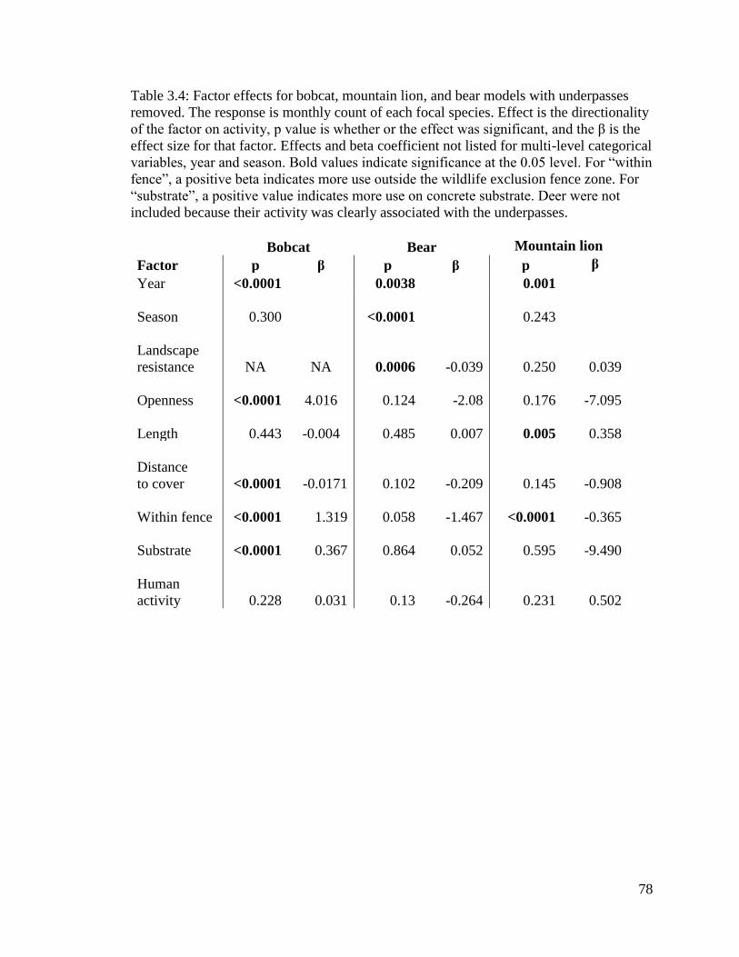
78
Table 3.4: Factor effects for bobcat, mountain lion, and bear models with underpasses
removed. The response is monthly count of each focal species. Effect is the directionality
of the factor on activity, p value is whether or the effect was significant, and the β is the
effect size for that factor. Effects and beta coefficient not listed for multi-level categorical
variables, year and season. Bold values indicate significance at the 0.05 level. For “within
fence”, a positive beta indicates more use outside the wildlife exclusion fence zone. For
“substrate”, a positive value indicates more use on concrete substrate. Deer were not
included because their activity was clearly associated with the underpasses.
Factor
Bobcat Bear Mountain lion
p β p β p β
Year <0.0001 0.0038 0.001
Season 0.300
<0.0001 0.243
Landscape
resistance NA NA 0.0006 -0.039 0.250 0.039
Openness <0.0001 4.016 0.124 -2.08 0.176 -7.095
Length 0.443 -0.004 0.485 0.007 0.005 0.358
Distance
to cover <0.0001 -0.0171 0.102 -0.209 0.145 -0.908
Within fence <0.0001 1.319 0.058 -1.467 <0.0001 -0.365
Substrate <0.0001 0.367 0.864 0.052 0.595 -9.490
Human
activity 0.228 0.031 0.13 -0.264 0.231 0.502

79
Table 3.5a: Count and activity of bobcat and mountain lion at each site. Count is the
number of detection events for a given species, irrespective of group size. Activity is the
count divided by the total survey days. “Act*30” is activity multiplied by 30 to estimate
the number of monthly detections at each site. “-“ indicates zero activity for clarity.
Bobcat Mountain Lion
Site Survey
nights Count Activity Act.*30 Count Activity Act*30
Woods-Culv 1746 295 0.169 5.07 0 - -
N3.1-Culv 1071 319 0.298 8.94 15 0.014 0.42
TjCk-Culv 1163 9 0.008 0.23 0 - 0.00
WatDist-Culv 1866 90 0.048 1.45 10 0.005 0.16
58N-Culv 1301 2 0.002 0.05 0 - -
58S-Culv 1422 57 0.040 1.20 0 - -
N8.5-Culv 1856 287 0.155 4.64 1 0.001 0.02
N9.1-Culv 1849 100 0.054 1.62 2 0.001 0.03
N10.0-Culv 1808 4 0.002 0.07 0 - -
RR-UP 711 55 0.077 2.32 2 0.003 0.08
SM-UP 207 13 0.063 1.88 2 0.010 0.29

80
Table 3.5b: Count and activity of deer and black bear at each site. Count is the number of
detection events for a given species, irrespective of group size. “act.” is the count divided
by the total survey days. “act*30” is activity multiplied by 30 to estimate the number of
monthly detections at each site. “-“ indicates zero activity for clarity.
Deer Bear
Site Survey
days Count Activity Act*30 Count Activity Act*30
Woods-Culv 1746 16 0.009 0.27 4 0.002 0.07
N3.1-Culv 1071 1 0.001 0.03 17 0.016 0.48
TjCk-Culv 1163 1 0.001 0.03 45 0.039 1.16
WatDist-Culv 1866 4 0.002 0.06 28 0.015 0.45
58N-Culv 1301 0 - - 14 0.011 0.32
58S-Culv 1422 0 - - 18 0.013 0.38
N8.5 1856 4 0.002 0.06 1 0.001 0.02
N9.1 1849 0 - - 0 - -
N10.0 1808 3 0.002 0.05 0 - -
RR-UP 711 343 0.482 14.47 15 0.021 0.63
SM-UP 207 238 1.150 34.49 0 - -
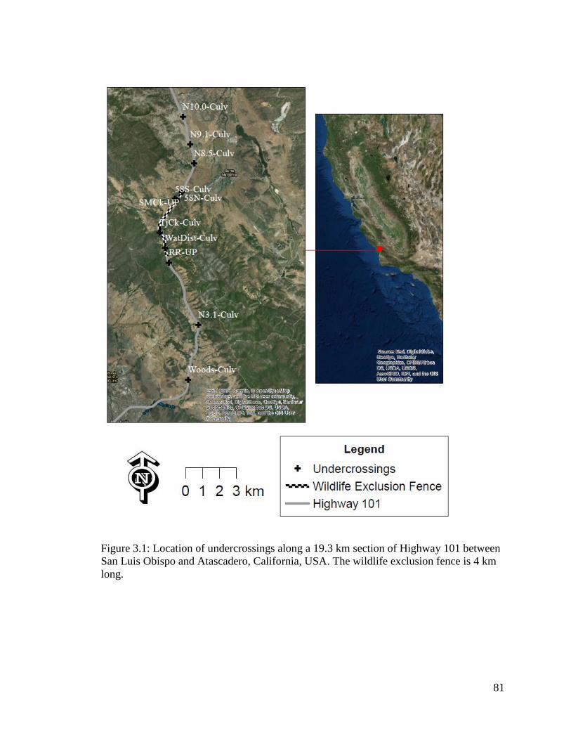
81
Figure 3.1: Location of undercrossings along a 19.3 km section of Highway 101 between
San Luis Obispo and Atascadero, California, USA. The wildlife exclusion fence is 4 km
long.
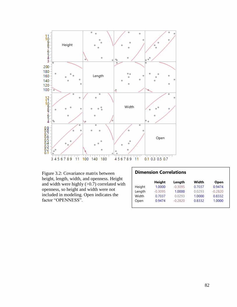
82
Figure 3.2: Covariance matrix between
height, length, width, and openness. Height
and width were highly (>0.7) correlated with
openness, so height and width were not
included in modeling. Open indicates the
factor “OPENNESS”.
Dimension Correlations
Height Length Width Open
Height 1.0000 -0.3095 0.7037 0.9474
Length -0.3095 1.0000 0.0293 -0.2820
Width 0.7037 0.0293 1.0000 0.8332
Open 0.9474 -0.2820 0.8332 1.0000

83
Figure 3.3: Monthly count of deer detections at each site, irrespective of group size. Deer
almost exclusively used the two underpasses (RR and SM). N=610.

84
Figure 3.4: Monthly count of bear at each site, irrespective of group size. N=142.

85
Figure 3.5: Monthly count of mountain lion at each site, irrespective of group size. N=32.

86
Figure 3.6: Monthly count of bobcat at each site, irrespective of group size. N=1231.

87
Figure 3.7: Monthly count of human at each site, irrespective of group size. N=188.

88
Figure 3.8: Focal species activity at each site. Bars are the average monthly count divided
by 30 to give an estimate for daily activity. RR and SM are both underpasses, the rest of
the sites are culverts.

89
REFERENCES
Alexander, S.M., and N.M. Waters. 2000. The effects of highway transportation
corridors on wildlife: a case study of Banff National Park. Transportation Research Part
C: Emerging Technologies, 8: 307-320.
Allen, T.D.H., M.P. Huijser, and D.W. Willey. 2013. Effectiveness of wildlife
guards at access roads. Wildlife Society Bulletin 37.2: 402-408.
Andis, A.Z., M.P. Huijser, and L. Broberg. 2017. Performance of arch-style road
crossing structures from relative movement rates of large mammals. Frontiers in Ecology
and Evolution 5: 122.
Arizona Department of Transportation. 2013. Wildlife escape measures. Arizona
Department of Transportation, Phoenix, Arizona, USA.
http://www.azdot.gov/docs/default-
source/planning/description_of_wildlife_escape_measures.pdf?sfvrsn=2
Bangs, E.E., T.N. Bailey, and M.F. Portner. 1989. Survival rates of adult female
moose on the Kenai Peninsula, Alaska. Journal of Wildlife Management 53: 557-563.
Barbour, M., T. Keeler-Wolf, and A.A. Schoenherr, editors. 2007. Terrestrial
vegetation of California. University of California Press.
Bashore, T.L., W.M. Tzilkowski, and E.D. Bellis. 1985. Analysis of deer-vehicle
collision sites in Pennsylvania. Journal of Wildlife Management 49: 769-774.
Beckmann, J.P., A.P. Clevenger, M.P. Huijser, and J.A. Hilty. 2010. Safe
passages. Highways, wildlife, and habitat connectivity. Island Press, Washington, D.C.,
USA.

90
Beier, P., D. Choate, and R.H. Barrett. 1995. Movement patterns of mountain
lions during different behaviors. Journal of Mammalogy 76: 1056-1070.
Belovsky, G. E. 1987. Extinction models and mammalian persistence. Pages 35-
58 in M. E. Soulé, editor. Viable populations for conservation. Cambridge University
Press, Cambridge, Massachusetts, USA.
Bissonette, J., and M. Hammer. 2000. Effectiveness of earthen return ramps in
reducing big game highway mortality in Utah. UTCFWRU Report Series 2000: 1-29.
Blincoe, L., A. Seay, E. Zaloshnja, T. Miller, E. Romano, S. Luchter, and R.
Spicer. 2002. The economic impact of motor vehicle crashes. U.S. Department of
Transportation National Highway Traffic Safety Administration, Washington, D.C.,
USA.
Bliss-Ketchum, L.L., P. Cramer, S. Gregory, S. Jacobson, M. Trask, S. Wray.
2016. The effect of artificial light on wildlife use of a passage structure. Biological
Conservation 199: 25-28.
Brown, J.H. 1986. Two decades of interaction between the Mac- Arthur-Wilson
model and the complexities of mammalian distributions. Biological Journal of the
Linnaean Society 28: 231-251.
California Department of Fish and Wildlife [CDFW]. CDFW website. Mule Deer
(Odocoileus hemionus). https://www.wildlife.ca.gov/Regions/6/Deer/Natural-History.
Chapman J.A. and G. Feldhamer. 1982. Wild Mammals of North America. Johns
Hopkins University Press, USA.

91
Chruszcz B., A.P. Clevenger, K. Gunson, and M. Gibeau. 2003. Relationships
among grizzly bears, highways and habitat in the Banff-Bow Valley, Alberta, Canada.
Canadian Journal of Zoology 81: 1378-1391.
Clevenger, A.P., A.T. Ford, and M.A. Sawaya. 2009. Banff wildlife crossings
project: integrating science and education in restoring population connectivity across
transportation corridors. Report for the Parks Canada Agency.
Clevenger, A.P., and M. Barrueto (eds). 2014. Trans‐Canada highway wildlife
and monitoring research, final report, part B: Research Prepared for Parks Canada
Agency, Radium Hot Springs, British Columbia.
Clevenger, A.P., and M. Barrueto. 2014. Trans‐Canada highway wildlife and
monitoring research, final report, part B: Research Prepared for Parks Canada Agency,
Radium Hot Springs, British Columbia.
Clevenger, A.P., and M.P. Huijser. 2011. Wildlife Crossing Structure Handbook
Design and Evaluation in North America. Report to the Federal Highway Administration,
Washington, DC, USA. No. FHWA-CFL/TD-11-003.
Clevenger, A.P., and N. Waltho. 1999. Dry drainage culvert use and design
considerations for small- and medium sized mammal movement across and major
transportation corridor. In: Evink, G.L., Garrett, P., Zeigler, D., Berry, J. (Eds.),
Proceedings of the International Conference on Wildlife Ecology and Transportation. FL-
ER-69-98. Florida Department of Transportation, Tallahassee, FL, pp. 263–277.
Clevenger, A.P., and N. Waltho. 2000. Factors influencing the effectiveness of
wildlife underpasses in Banff National Park, Alberta, Canada. Conservation Biology
14.1: 47-56.

92
Clevenger, A.P., and N. Waltho. 2005. Performance indices to identify attributes
of highway crossing structures facilitating movement of large mammals. Biological
Conservation 121: 453-464.
Clevenger, A.P., B. Chruszcz, and K.E. Gunson. 2001. Highway mitigation
fencing reduces wildlife-vehicle collisions. Wildlife Society Bulletin 29: 646-653.
Clevenger, A.P., B. Chruszcz, K. Gunson, & M. Brumfit. 2002. Highway
mitigation monitoring: Three Sisters Parkway interchange. Report for Alberta Sustainable
Resource Development, Canmore, Alberta, Canada.
Cramer, P.C., and J.A. Bissonette. 2005. Wildlife crossings in North America: the
state of the science and practice. IN: Proceedings of the 2005 International Conference on
Ecology and Transportation, Eds. Irwin CL, Garrett P, McDermott KP. Center for
Transportation and the Environment, North Carolina State University, Raleigh, NC: pp.
442-447.
Cramer, P.C., and K.M. Portier. 2001. Modeling Florida panther movements in
response to human attributes of the landscape and ecological settings. Ecological
Modeling 140: 51-80.
Crooks K.R., and M.E. Soulé. 1999. Mesopredator release and avifaunal
extinctions in a fragmented system. Nature 400: 563-566.
Crooks, K.R. 2002. Relative sensitivities of mammalian carnivores to habitat
fragmentation. Conservation Biology 16: 488-502.
deVos, J.C., Jr ., M.R. Conover, and N.E. Headrick, editors. 2003. Mule deer
conservation: issues and management strategies. Berryman Institute Press, Utah State
University, Logan, USA.

93
Dodd Jr., C.K., W.J. Barichivich, and L.L Smith. 2004. Effectiveness of a barrier
wall and culverts in reducing wildlife mortality on a heavily traveled highway in Florida.
Biological Conservation 118: 619-631.
Donaldson, B., Y. Kweon, and L.N. Lloyd. 2015. An evaluation of roadside
activity and behavior of deer and black bear to determine mitigation strategies for animal-
vehicle collisions. No. FHWA/VTRC 16-R4. Virginia Transportation Research Council.
Ernest, H.B., W.M. Boyce, V.C. Bleich, B. May, S.J. Stiver, and S.G. Torres.
2003. Genetic structure of mountain lion (Puma concolor) populations in California.
Conservation Genetics 4: 353.
Falk, N.W., H.B. Graves, and E.D. Bellis. 1978. Highway right-of-way fences as
deer deter- rents. Journal of Wildlife Management 42: 646-650.
Forman, R.T. 2000. Estimate of the area affected ecologically by the road system
in the United States. Conservation biology 14: 31-35.
Forman, R.T., and L.E. Alexander. 1998. Roads and their major ecological
effects. Annual Review of Ecology and Systematics 29: 207-231.
Forman, R.T., and R.D. Deblinger. 2000. The ecological road-effect zone of a
Massachusetts (U.S.A.) suburban highway. Conservation Biology 14: 36-46.
Forman, R.T.T., J.B. Sperling, A.P. Clevenger, V.H. Dale, L.F. France, C.R.
Goldman, K. Heanue, J.A. Jones, F.J. Swanson, T. Turrentine, and T.C. Winter. 2003.
Road ecology: science and solutions. Island Press, Washington, D.C., USA.
Foster, M.L., and S.R. Humphrey. 1995. Use of highway underpasses by Florida
panthers and other wildlife. Wildlife Society Bulletin 23: 95-100.

94
Gagnon, J.W., C.D. Loberger, S.C. Sprague, M. Priest, K. Ogren, S. Boe, E.
Kombe, and R. E. Schweinsburg. 2013. Evaluation of desert bighorn sheep overpasses
along US Highway 93 in Arizona, USA. Proceedings of the 2013 International
Conference on Ecology and Transportation.
Gagnon, J.W., T.C. Theimer, N.L. Dodd, S. Boe, R.E. Schweinsburg. 2007.
Traffic volume alters elk distribution and highway crossings in Arizona. Journal of
Wildlife Management 71.7: 2318-2323.
Garbutt, H. 2009. Wildlife-vehicle mitigation on northeastern Ontario highways.
Ontario Ministry of Transportation.
Glista, D.J., T.L. DeVault, and J.A. DeWoody. 2009. A review of mitigation
measures for reducing wildlife mortality on roadways. Landscape and Urban Planning
91.1: 1-7.
Grilo, C., J.A. Bissonette, and M. Santos-Reis. 2008. Response of carnivores to
existing highway culverts and underpasses: implications for road planning and
mitigation. Biodiversity and Conservation 17: 1685-1699.
Harestad, A.S. and F.L. Bunnel. 1979. Home range and body weight‐a
reevaluation. Ecology 60(2): 389-402.
Harris, L.D., and J. Scheck. 1991. From implications to applications: the dispersal
corridor principle applied to the conservation of biological diversity. Nature Conservation
2: 189-220.
Hemker, T.P., F.G. Lindzey, and B.B. Ackerman. 1984. Population characteristics
and movement patterns of cougars in southern Utah. Journal of Wildlife Management.
48: 1275-1284.
95
Hornocker, M.G., and H.S. Hash. 1981. Ecology of the wolverine in northwestern
Montana. Canadian Journal of Zoology 59: 1286-1301.
Huijser, M.P., A.V. Kociolek, T.D.H. Allen, P. McGowen, P.C. Cramer, and M.
Venner. 2015. Construction guidelines for wildlife fencing and associated escape and
lateral access control measures.
http://onlinepubs.trb.org/onlinepubs/nchrp/docs/NCHRP25- 25(84).
Huijser, M.P., J. Purdum, W. Camel-Means, and E. Fairbank. 2013. US 93 Post-
construction wildlife- vehicle collision and wildlife monitoring and research on the
Flathead Indian Reservation between Evaro and Polson, Montana, Quarterly Report
2013-3. Report for the Montana Department of Transportation. Helena, MT.
Huijser, M.P., J.W. Duffield, A.P. Clevenger, R.J. Ament, and P.T. McGowen.
2009. Cost-benefit analyses of mitigation measures aimed at reducing collisions with
large ungulates in the United States and Canada: A decision support tool. Ecology and
Society,14.2 Article 15.
Huijser, M.P., P.T. McGowen, J. Fuller, J.A., Hardy, & A. Kociolek. 2007.
Wildlife-vehicle collision reduction study: Report to Congress (No. FHWA-HRT-08-
034).
Huijser, M.P., W. Camel-Means, E.R. Fairbank, J.P. Purdum, T.D.H. Allen, A.R.
Hardy, J. Graham, J.S. Begley, P. Basting, and D. Becker. 2016. US 93 North Post-
Construction Wildlife-Vehicle Collision and Wildlife Crossing Monitoring on the
Flathead Indian Reservation between Evaro and Polson, Montana. Report for the
Montana Department of Transportation.
96
Hurlbert, S.H., 1984. Pseudoreplication and the design of ecological field
experiments. Ecological Monographs 54(2): 187-211.
Jennings, M.K. 2013. Landscape dynamics in Southern California: Understanding
mammalian carnivore response to fire and human development. [Ph.D. Dissertation].
University of California, Davis and San Diego State University.
Jones, M.E. 2000. Road upgrade, road mortality and remedial measures: impacts
on a population of eastern quolls and Tasmanian devils. Wildlife research 27(3): 289-296.
Kansas, J.L., and R.M. Raines. 1990. Methodologies used to assess the relative
importance of ecological land classification units to black bears in Banff National Park,
Alberta. International Conference on Bear Research and Management 8: 155–160.
Knapp, K.K., X. Yi, T. Oakasa, W. Thimm, E. Hudson, and C. Rathmann. 2004.
Deer–vehicle crash countermeasure toolbox: a decision and choice resource. Midwest
Regional University Transportation Center, Madison, Wisconsin, USA.
Koehler, G.M., and M.G. Hornocker. 1991. Seasonal resource use among
mountain lions, bobcats, and coyotes. Journal of Mammalogy 72: 391–396.
Kruidering, A.M., G. Veenbaas, R. Kleijberg, G.Koot, Y. Rosloot, and E. van
Jaarsveld. 2005. Leidraad faunavoorzieningen bij wegen. Rijkswaterstaat, Dienst Weg-en
Waterbouwkunde, Delft, The Netherlands.
Lambert, D. 1992. Zero-inflated Poisson regression, with an application to defects
in manufacturing. Technometrics 34.1: 1-14.
Lee, J.S., E.W. Ruell, E.E. Boydston, L.M. Lyren, R.S. Alonso, J.L. Troyer, K.R.
Crooks, and S. VandeWoude. 2012. Gene flow and pathogen transmission among

97
bobcats (Lynx rufus) in a fragmented urban landscape. Molecular Ecology 21: 1617-
1631.
Little, S.J., R.G. Harcourt, and A.P. Clevenger. 2002. Do wildlife passages act as
prey traps? Biological Conservation 107: 135-145.
Loberger, C., J.S. Gagnon. M. Sprague, M. Priest and R. Schweinsburg. 2013.
Evaluation of a wildlife fencing retrofit along Interstate-17: adding 1.2 meters (4’) to
interstate right-of-way fence reduced elk-vehicle collisions by 100%. Proceedings of the
2013 International Conference on Ecology and Transportation (ICOET 2013), Phoenix,
Arizona, USA.
Lyons, A.L., W.L. Gaines, and C. Servheen. 2003. Black bear resource selection
in the northeast Cascades, Washington. Biological Conservation 113: 55– 62.
Maehr, D.S., E.D. Land, and J.C. Roof. 1991. Social ecology of Florida panthers.
National Geographic Research Explorers 7: 414-431.
Main, M.B. and B.E. Coblentz. 1990. Sexual segregation among ungulates: a
critique. Wildlife Society Bulletin 18: 204-210.
Main, M.B. and B.E. Coblentz. 1996. Sexual segregation in Rocky Mountain
Mule Deer. Journal of Wildlife Management 60(3): 497-507.
Mastro, L.L., M.R. Conover, and S.N. Frey. 2008. Deer-vehicle collision
prevention techniques. Human-Wildlife Conflicts 2: 80-92.
McCollister M.F., F.T. Van Manen. 2010. Effectiveness of wildlife underpass and
fencing to reduce wildlife-vehicle collisions. Journal of Wildlife Management 74: 1722-
1731.

98
Meese, R. J., F.M. Shilling, and J.Quinn. 2009. Wildlife crossings guidance
manual. California Department of Transportation, Sacramento.
New York State Department of Motor Vehicles Internet Office. 2006. Driver’s
Manual.
Ng, S., J.W. Dole, R.M. Sauvajot, S.P.D. Riley, and T.J. Valone. 2004. Use of
highway undercrossing by wildlife in southern California. Biological Conservation 115:
499–507.
Noss, R. F., and A. Cooperrider. 1994. Saving nature's legacy: protecting and
restoring biodiversity. Island Press, Washington, D.C., USA.
Perrine, J.D. 2015. Assessment of the wildlife-exclusion infrastructure in the
Tassajara Creek Region of Highway 101 in San Luis Obispo County. California
Department of Transportation.
Perrine, J.D. and S. Snyder. 2011. Documenting Wildlife Distribution and
Activity along Highway 101 between San Luis Obispo and Atascadero. California
Department of Transportation, contract 06A1337. 51 pages + appendices.
Poessel, S.A., C.L. Burdett, E.E. Boydston, L. M. Lyren, R. S. Alonso, R. N.
Fisher, and K. R. Crooks. 2014. Roads influence movement and home ranges of a
fragmentation-sensitive carnivore, the bobcat, in an urban landscape. Biological
Conservation 180: 224-232.
Puglisi, M.J., J.S. Lindzey, and E.D. Bellis. 1974. Factors associated with
highway mortality of white-tailed deer. Journal of Wildlife Management 799-807.
Reed, D.F., T.N. Woodard, T.M. Pojar. 1975. Behavioral response of mule deer to
a highway underpass. Journal of Wildlife Management 39: 361–367.

99
Riley, S. P., R. M. Sauvajot, T. K. Fuller, E. C. York, D. A. Kamradt, C. Bromley,
and R. K. Wayne. 2003. Effects of urbanization and habitat fragmentation on bobcats and
coyotes in southern California. Conservation Biology 17: 566-576.
Riley, S.P., J.P. Pollinger, R. M. Sauvajot, E. C. York, C. Bromley, T. K. Fuller,
and R. K. Wayne. 2006. A southern California freeway is a physical and social barrier to
gene flow in carnivores. Molecular Ecology 15: 1733-1741.
Riley, S.P.D., E.E. Boydston, K.R. Crooks, L.M. Lyren. 2010. Bobcats (Lynx
rufus). In: Gehrt, S.D., S.P.D. Riley, B.L. Cypher (Eds.), Urban Carnivores: Ecology,
Conflict, and Conservation. Johns Hopkins University Press, Baltimore, Maryland, USA,
pp. 120–139.
Ripple, W.J., J.A. Estes, R.L. Beschta, C.C. Wilmers, E.G., Ritchie, M.
Hebblewhite, M., Berger, J., Elmhagen, B., Letnic, M., M.P. Nelson, and O.J. Schmitz.
2014. Status and ecological effects of the world’s largest carnivores. Science
343:1241484.
Rodriguez, A., G. Crema, and M. Delibes. 1996. Use of non-wildlife passages
across a high speed railway by terrestrial vertebrates. Journal of Applied Ecology 33:
1527-1540.
Roemer, G.W., M.E. Gompper, and B.V. Valkenburgh. 2009. The ecological role
of the mammalian mesocarnivore. BioScience 59: 165-173.
Romin, L.A., and J.A. Bissonette. 1996. Deer vehicle collisions: status of state
monitoring activities and mitigation efforts. Wildlife Society Bulletin 24: 276-283.

100
Rosell, C., J. Parpal, R. Campeny, S. Jove, A. Pasquina, and J. M. Velasco. 1997.
Mitigation of barrier effect on linear infrastructures on wildlife. Ministry of
Transportation, Public Works and Water Management, Delft, The Netherlands 367-372.
Rytwinski, T., K. Soanes, J.A. Jaeger, L. Fahrig, C.S. Findlay, J. Houlahan, R.
van der Ree, E.A. van der Grift. 2016. How effective is road mitigation at reducing road-
kill? A meta-analysis. PLoS One 11.11: e0166941.
Sargeant, G.A., D.H. Johnson, and W.E. Berg. 1998. Interpreting carnivore scent-
station surveys. Journal of Wildlife Management 62: 1235–1245.
Shilling, F.M., and D.P. Waetjen. 2012. The Road Effect Zone GIS Model.
Institute of Transportation Studies, University of California, Davis.
Siemers, J.L., K.R. Wilson, and S. Baruch-Mordo. 2015. Monitoring wildlife-
vehicle collisions: analysis and cost–benefit of escape ramps for deer and elk on US
Highway 550. Department of Fish, Wildlife, and Conservation Biology, Colorado State
University Fort Collins, Colorado, USA. Report No. CDOT-2015-05.
Siepel, N.R., J.D. Perrine, L.K. Schicker, and M. Robertson. 2013. Saving lives
and training the next generation: State Route 101 wildlife corridor safety project.
Proceedings of the 2013 International Conference on Ecology and Transportation
(ICOET 2013).
Smith, J.A., J.P. Suraci, M. Clinchy, A. Crawford, D. Roberts, L.Y. Zanette and
C.C. Wilmers, 2017. Fear of the human ‘super predator’ reduces feeding time in large
carnivores. Proceedings of the Royal Society B, 284(1857), p. 20170433.
101
Snyder, S.A. 2014. Examining the impacts of State Route 101 on wildlife using
road kill surveys and remote cameras. Master’s Thesis, California Polytechnic
University San Luis Obispo.
Sommer, M.L., R.L. Barboza, R.A. Botta, E.B. Kleinfelter, M.E. Schauss and J.R.
Thompson. 2007. Habitat guidelines for mule deer: California woodland chaparral
ecoregion. Mule Deer Working Group, Western Association of Fish and Wildlife
Agencies.
Sparks, J.L., J.E. Gates. 2017. Seasonal and regional animal use of drainage
structures to cross under roadways. Human-Wildlife Interactions 11(2): 182-191.
Spencer, W.D., P. Beier, K. Penrod, K. Winters, C. Paulman, H. Rustigian-
Romsos, J. Strittholt, M. Parisi, and A. Pettler. 2010. California Essential Habitat
Connectivity Project: A Strategy for Conserving a Connected California. Prepared for
California Department of Transportation, California Department of Fish and Game, and
Federal Highways Administration.
Stickles, J.H., D.B. Stone, C.S. Evans, K.V. Miller, R.J. Warren, D.A. Osborn,
and C.H. Killmaster. 2015. Using deer-vehicle collisions to map white-tailed deer
breeding activity in Georgia. Journal of the Southeastern Association of Fish and
Wildlife Agencies 2: 202-207.
Stoner, D. 1925. The toll of the automobile. Science 61: 56-58.
Stull, D.W., W.D. Gulsby, J.A. Martin, G.J. D'Angelo, G.R. Gallagher, D.A.
Osborn, R.J. Warren, and K.V. Miller. 2011. Comparison of fencing designs for
excluding deer from roadways. Human-Wildlife Interactions 5: 47-57.

102
Taber, R.D. and R.F. Dasmann. 1958. The black-tailed deer of the chaparral: its
life history and management in the North Coast Range of California (No. 8). California
Department of Fish and Game, Game Management Branch, Sacramento, California.
Thorne, J., and P. Huber. 2011. GIS modeling of landscape permeability for
wildlife on the Highway 101 corridor between San Luis Obispo and Atascadero. Final
project report to California Department of Transportation.
Thorne, J., D. Cameron, V. Jignour. 2002. Wildlands Conservation in the Central
Coast region of California. Report to the California Wilderness Coalition.
Thorne, J.H., D. Cameron, and J.F. Quinn. 2006. A conservation design for the
central coast of California and the evaluation of mountain lion as an umbrella species.
Natural Areas Journal 26: 137-148.
Van der Zee, F. F., J. Wiertz, C.J. Ter Braak, R.C. Apeldoorn. 1992. Landscape
change as a possible cause of the badger Meles meles L. decline in the Netherlands.
Biological Conservation 61.1: 17-22.
Van Dyke F.G, R.H. Brocke, and H.G. Shaw. 1986. Use of road track counts as
indices of mountain lion presence. Journal of Wildlife Management 50: 102-109.
Van Wieren, S.E., and P.B. Worm. 2001. The use of a motorway wildlife
overpass by large mammals. Netherlands Journal of Zoology 51: 97-105.
Yanes, M., J. M. Velasco, and F. Suarez. 1995. Permeability of roads and
railways to vertebrates: the importance of culverts. Biological Conservation 71: 217-222.