
Convex Optimization and Modeling
Convex Optimization
Fourth lecture, 05.05.2010
Jun.-Prof. Matthias Hein

Reminder from last time
Convex functions:
• first-order condition: f(y) ≥ f(x) + 〈∇f |x, y − x〉,
• second-order condition: Hessian Hf positive semi-definite,
• convex functions are continuous on the relative interior,
• a function f is convex ⇐⇒ the epigraph of f is a convex set.
Extensions:
• quasiconvex functions have convex sublevel sets,
• log-concave/convex f : log f is concave/convex.
1

Program of today/next lecture
Optimization:
• general definition and terminology
• convex optimization
• quasiconvex optimization
• linear optimization (linear programming (LP))
• quadratic optimization (quadratic programming (QP))
• geometric programming
• generalized inequality constraints
• semi-definite and cone programming
2

Mathematical Programming
Definition 1. A general optimization problem has the form
minx∈D
f(x),
subject to: gi(x) ≤ 0, i = 1, . . . , r
hj(x) = 0, j = 1, . . . , s.
• x is the optimization variable, f the objective (cost) function,
• x ∈ D is feasible if the inequality and equality constraints hold at x.
• the optimal value p∗ of the optimization problem
p∗ = inf{f(x) |x feasible }.
p∗ = −∞: problem is unbounded from below,
p∗ = ∞: problem is infeasible.
3
Mathematical Programming II
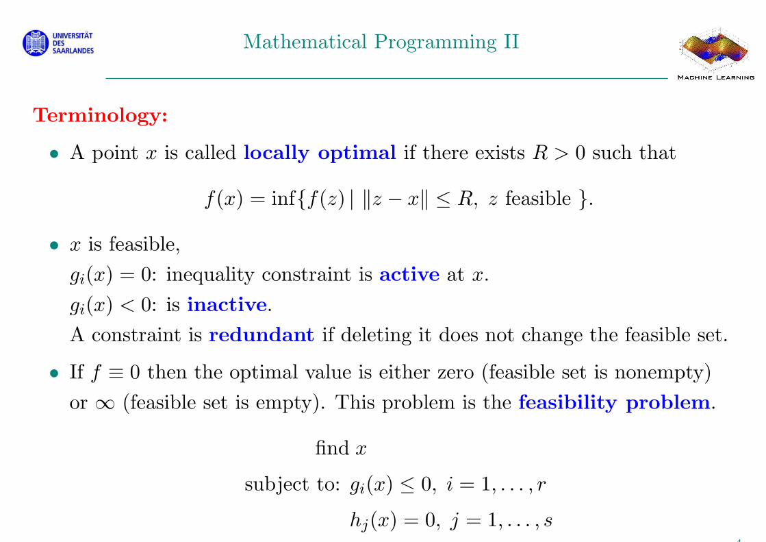
Terminology:
• A point x is called locally optimal if there exists R > 0 such that
f(x) = inf{f(z) | ‖z − x‖ ≤ R, z feasible }.
• x is feasible,
gi(x) = 0: inequality constraint is active at x.
gi(x) < 0: is inactive.
A constraint is redundant if deleting it does not change the feasible set.
• If f ≡ 0 then the optimal value is either zero (feasible set is nonempty)
or ∞ (feasible set is empty). This problem is the feasibility problem.
find x
subject to: gi(x) ≤ 0, i = 1, . . . , r
hj(x) = 0, j = 1, . . . , s4

Equivalent Problems
Equivalent problems: Two problems are called equivalent if one can
obtain from the solution of one problem the solution of the other problem
and vice versa.
Transformations which lead to equivalent problems:
• Slack variables: gi(x) ≤ 0 ⇐⇒ ∃ si ≥ 0 such that gi(x) + si = 0.
minx∈Rn, s∈Rr
f(x),
subject to: gi(x) + si = 0, i = 1, . . . , r
si ≥ 0, i = 1, . . . , r
hj(x) = 0, j = 1, . . . , s,
which has variables x ∈ Rn and s ∈ R
r.
5

Equivalent Problems II
Transformations which lead to equivalent problems II:
• Epigraph problem form of the standard optimization problem:
minx∈Rn, t∈R
t,
subject to: f(x) − t ≤ 0,
gi(x) ≤ 0, i = 1, . . . , r
hj(x) = 0, j = 1, . . . , s,
which has variables x ∈ Rn and t ∈ R.
6
Convex Optimization
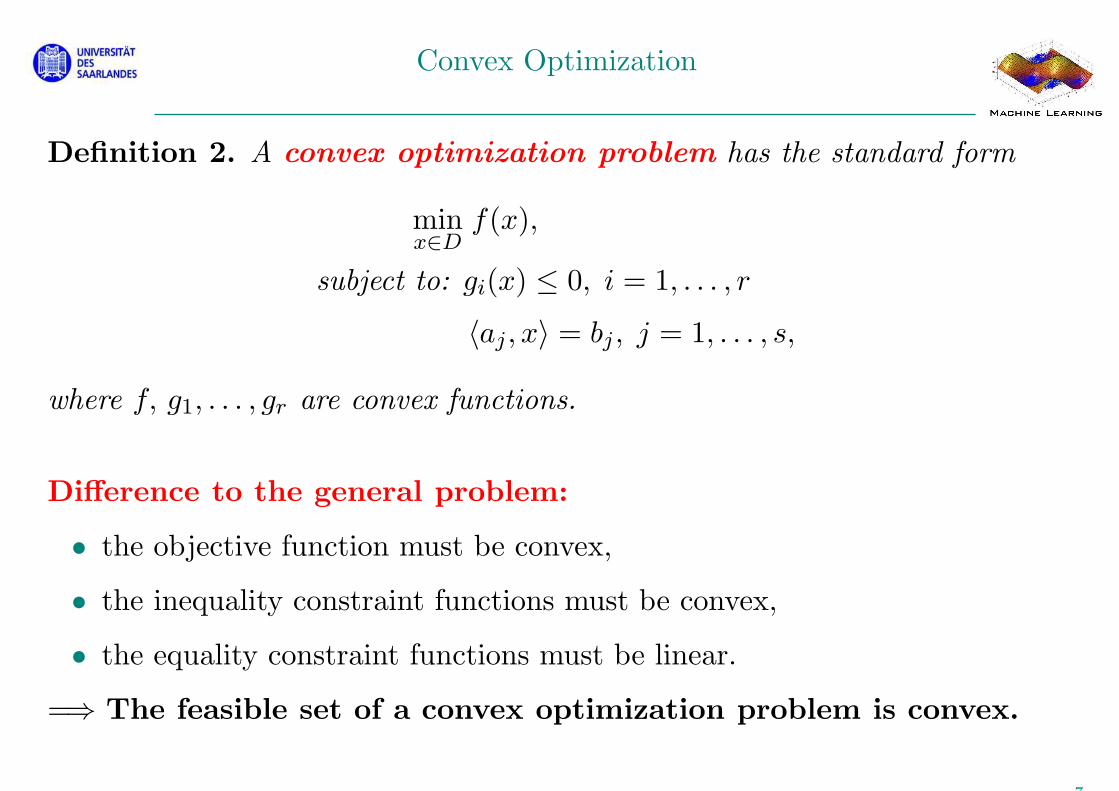
Definition 2. A convex optimization problem has the standard form
minx∈D
f(x),
subject to: gi(x) ≤ 0, i = 1, . . . , r
〈aj , x〉 = bj , j = 1, . . . , s,
where f, g1, . . . , gr are convex functions.
Difference to the general problem:
• the objective function must be convex,
• the inequality constraint functions must be convex,
• the equality constraint functions must be linear.
=⇒ The feasible set of a convex optimization problem is convex.
7

Convex Optimization II
Local and global minima
Theorem 1. Any locally optimal point of a convex optimization problem is
globally optimal.
Proof. Suppose x is locally optimal, that means x is feasible and ∃R > 0,
f(x) = inf{f(z) | ‖z − x‖ ≤ R, z feasible }.
Assume x is not globally optimal =⇒ ∃ feasible y such that f(y) < f(x).
f(λx + (1 − λ)y) ≤ λf(x) + (1 − λ)f(y) < f(x),
for any 0 < λ < 1 =⇒ x is not locally optimal �. 2
Locally optimal points of quasiconvex problems are not generally globally
optimal.8

First-Order Condition for Optimality
First-Order Condition for Optimality:
Theorem 2. Suppose f is convex and continuously differentiable, Then x is
optimal if and only if x is feasible and
〈∇f |x, y − x〉 ≥ 0, ∀ y ∈ X.
Proof: Suppose x ∈ X and 〈∇f |x, y − x〉 ≥ 0, ∀ y ∈ X =⇒ f(y) ≥ f(x)
for all y ∈ X (first order condition).
Suppose that x is optimal but there is y ∈ X such that
〈∇f |x, y − x〉 < 0.
Let z = ty + (1− t)x with t ∈ [0, 1]. Then z(t) is feasible for all t ∈ [0, 1] and,
∂f
∂t
∣
∣
∣
t=0= 〈∇f |x, y − x〉 < 0,
so that for t ≪ 1 we have f(y) < f(x) �.9
First-Order Condition for Optimality
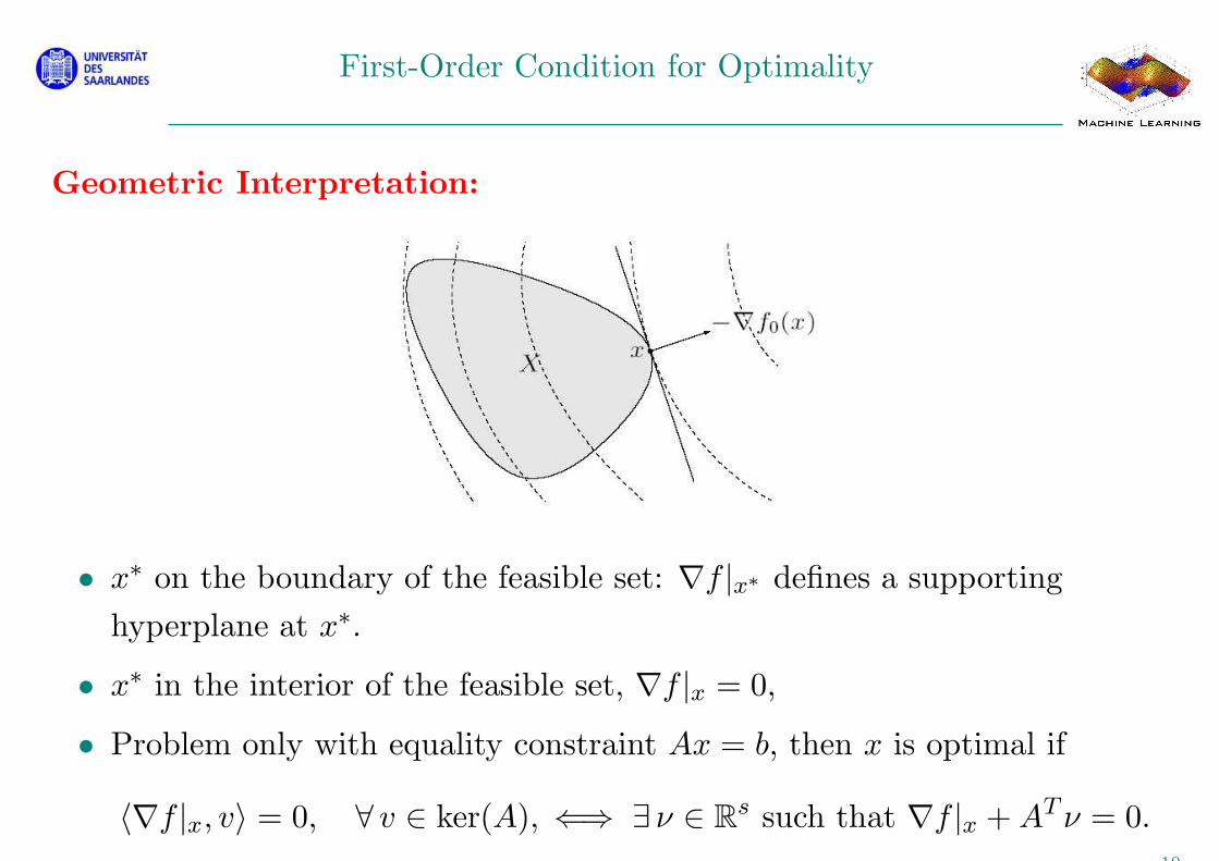
Geometric Interpretation:
• x∗ on the boundary of the feasible set: ∇f |x∗ defines a supporting
hyperplane at x∗.
• x∗ in the interior of the feasible set, ∇f |x = 0,
• Problem only with equality constraint Ax = b, then x is optimal if
〈∇f |x, v〉 = 0, ∀ v ∈ ker(A), ⇐⇒ ∃ ν ∈ Rs such that ∇f |x + AT ν = 0.
10

Equivalent convex problems
Equivalent convex problems
minx∈D
f(x),
subject to: gi(x) ≤ 0, i = 1, . . . , r
〈aj , x〉 = bj , j = 1, . . . , s,
• Elimination of equality constraints:
Let F ∈ Rn×k and x0 ∈ R
n such that
Ax = b ⇐⇒ x = Fz + x0, z ∈ Rk,
min f(Fz + x0),
subject to: gi(Fz + x0) ≤ 0, i = 1, . . . , r
This problem has only n − dim(ran(A)) or dim(kerA) variables.
11

Equivalent convex problems II
Transformations which preserve convexity
• Introduction of slack variables,
• Introduction of new linear equality constraints,
• Epigraph problem formulation,
• Minimization over some variables.
12

Quasiconvex Optimization
Definition 3. A quasiconvex optimization problem has the standard
form
minx∈D
f(x),
subject to: gi(x) ≤ 0, i = 1, . . . , r
〈aj , x〉 = bj , j = 1, . . . , s,
where f is quasiconvex and g1, . . . , gr are convex functions.
Quasiconvex inequality functions can be reduced to convex inequality
functions with the same 0-sublevel set.
13

Quasiconvex Optimization II
Theorem 3. Let X denote the feasible set of a quasiconvex optimization
problem with a differentiable objective function f . Then x ∈ X is optimal if
〈∇f |x, y − x〉 > 0, ∀ y ∈ X, y 6= x.
A quasi-convex function with ∇f |x0= 0 but x0 is not optimal.
14
Quasiconvex Optimization III
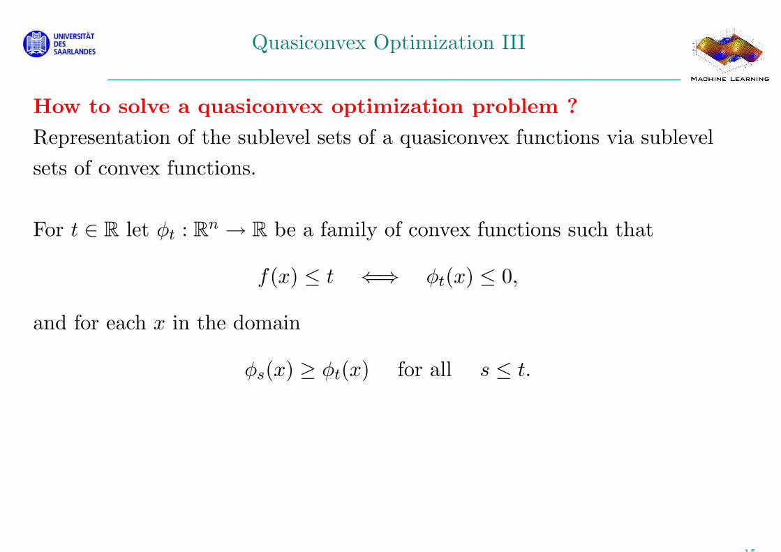
How to solve a quasiconvex optimization problem ?
Representation of the sublevel sets of a quasiconvex functions via sublevel
sets of convex functions.
For t ∈ R let φt : Rn → R be a family of convex functions such that
f(x) ≤ t ⇐⇒ φt(x) ≤ 0,
and for each x in the domain
φs(x) ≥ φt(x) for all s ≤ t.
15

Quasiconvex Optimization IV
Solve the convex feasibility problem:
find x
subject to: φt(x) ≤ 0
gi(x) ≤ 0, i = 1, . . . , r
Ax = b,
Two cases:
• a feasible point exists =⇒ optimal value p∗ ≤ t
• problem is infeasible =⇒ optimal value p∗ ≥ t
Solution procedure:
• assume p∗ ∈ [a, b] and use bisection t = b+a2
,
• after k-th iteration interval has length b−a2k ,
• k = log2b−a
ǫiterations in order to find an ǫ-approximation of p∗.
16

Linear Programming
Definition 4. A general linear optimization problem (linear program
(LP)) has the form
min 〈c, x〉
subject to: Gx � h,
Ax = b,
where c ∈ Rn, G ∈ R
r×n with h ∈ Rr and A ∈ R
s×n with b ∈ Rs.
A linear program is a convex optimization problem with
• affine cost function and linear inequality constraints
• The feasible set is a polyhedron.
17

Linear Programming II
The standard form of an LP
minx∈Rn
〈c, x〉
subject to: Ax = b,
x � 0.
Conversion of a general linear program into the standard form:
• introduce slack variables,
• decompose x = x+ − x− with x+ � 0 and x− � 0.
minx∈Rn, s∈Rr
〈c, x〉
subject to: Gx + s = h,
Ax = b,
s � 0.
minx+∈Rn, x−∈Rn, s∈Rr
⟨
c, x+⟩
−⟨
c, x−⟩
subject to: Gx+ − Gx− + s = h,
Ax+ − Ax− = b,
s � 0, x+ � 0, x− � 0.18

Examples of LPs
The diet problem:
• A healthy diet has m different nutrients in quantities at least equal to
b1, . . . , bm,
• n different kind of food and x1, . . . , xn is the amount of them and has
costs c1, . . . , cn,
• The food j contains an amount of aij of nutrient i.
• Goal: find the cheapest diet that satisfies the nutritional requirements
min 〈c, x〉
subject to: Ax � b,
x � 0.
19

Examples of LPs II
Chebychev center of a polyhedron:
• find the largest Euclidean ball and its center which fits into a polyhedron
P = {x ∈ Rn | 〈ai, x〉 ≤ bi, i = 1, . . . , r}.
• constraint that the ball B = {xc + u | ‖u‖ ≤ R} lies in one half-space
∀u ∈ Rn, ‖u‖ ≤ R =⇒ 〈ai, xc + u〉 ≤ bi.
With sup{〈ai, u〉 | ‖u‖ ≤ R} = R ‖ai‖2the constraint can be rewritten as
〈ai, xc〉 + R ‖ai‖2≤ bi.
Thus the problem can be reformulated as
maxx∈Rn, R∈R
R
subject to: 〈ai, xc〉 + R ‖ai‖2≤ bi, i = 1, . . . , r.
20

Quadratic Programming
Definition 5. A general quadratic program (QP) has the form
min1
2〈x, Px〉 + 〈q, x〉 + c
subject to: Gx � h,
Ax = b,
where P ∈ Sn+, G ∈ R
r×n and A ∈ Rs×n.
With quadratic inequality constraints:
1
2〈x, Pix〉 + 〈qi, x〉 + ci ≤ 0, with Pi ∈ Sn
+, i = 1, . . . , r
we have a quadratically constrained quadratic program (QCQP).
LP ⊂ QP ⊂ QCQP.21

Examples for a QP
• Least Squares: Minimizing ‖Ax − b‖2
2=
⟨
x,AT Ax⟩
− 2 〈b,Ax〉 + 〈b, b〉
is an unconstrained QP. Analytical solution: x = A†b.
• Linear Program with random cost:
min 〈c, x〉
subject to: Gx � h,
Ax = b,
– c is random with: c = E[c], and
covariance Σ = E[(c − c)(c − c)T ].
– the cost 〈c, x〉 is random with mean
E[〈c, x〉] = 〈c, x〉 and variance
Var[〈c, x〉] = 〈x,Σx〉 .
Risk-sensitive cost: E[〈c, x〉] + γ Var[〈c, x〉] = 〈c, x〉 + γ 〈x,Σx〉,
We get the following QP:
min 〈c, x〉 + γ 〈x,Σx〉
subject to: Gx � h,
Ax = b.22

Second-order cone problem
Definition 6. A second-order cone problem (SOCP) has the form
min 〈f, x〉
subject to: ‖Aix + bi‖ ≤ 〈ci, x〉 + di, i = 1, . . . , r
Fx = g,
where Ai ∈ Rni×n, b ∈ R
ni and F ∈ Rp×n.
‖Ax + b‖2≤ 〈c, x〉 + d,
with A ∈ Rk×n is a second-order cone constraint. The function
Rn → R
k+1, x 7→ (Ax + b, 〈c, x〉 + d)
is required lie in the second order cone in Rk+1.
ci = 0, 1 ≤ i ≤ r: reduces to a QCQP, Ai = 0, 1 ≤ i ≤ r: reduces to a LP.
QCQP ⊂ SOCP.
23

Example for SOCP
Robust linear programming: robust wrt to uncertainty in parameters,
• Consider the linear program
min 〈c, x〉
subject to: 〈ai, x〉 ≤ bi,
• ai ∈ Ei = {ai + Piu | ‖u‖2≤ 1} where Pi ∈ Sn
+,
min 〈c, x〉
subject to: 〈ai, x〉 ≤ bi, ∀ ai ∈ Ei
• sup{〈ai, x〉 | ai ∈ Ei} = 〈ai, x〉 + ‖Pix‖2. Thus,
〈ai, x〉 + ‖Pix‖2≤ bi (second-order constraint) .
min 〈c, x〉
subject to: 〈ai, x〉 + ‖Pix‖2≤ bi.
24

Example for SOCP II
Linear Programming with random constraints: ai ∼ N(ai,Σi).
The linear program with random constraints
min 〈c, x〉
subject to: P(〈ai, x〉 ≤ bi) ≥ η, i = 1, . . . , r,
can be expressed as SOCP
min 〈c, x〉
subject to: 〈ai, x〉 + Φ−1(η)
∥
∥
∥
∥
Σ1
2
i x
∥
∥
∥
∥
2
≤ bi, i = 1, . . . , r,
where φ(z) = P(X ≤ z) with X ∼ N(0, 1).
25
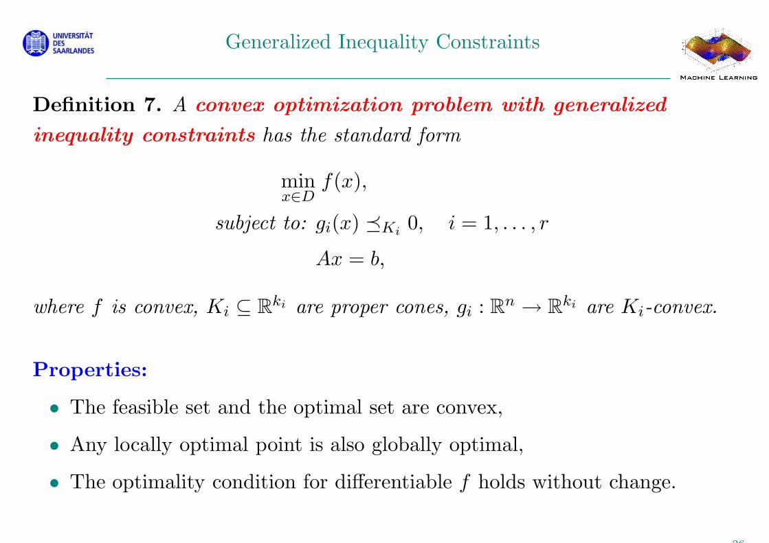
Generalized Inequality Constraints
Definition 7. A convex optimization problem with generalized
inequality constraints has the standard form
minx∈D
f(x),
subject to: gi(x) �Ki0, i = 1, . . . , r
Ax = b,
where f is convex, Ki ⊆ Rki are proper cones, gi : R
n → Rki are Ki-convex.
Properties:
• The feasible set and the optimal set are convex,
• Any locally optimal point is also globally optimal,
• The optimality condition for differentiable f holds without change.
26

Conic Program
Definition 8. A conic-form problem or conic program has the form
min 〈c, x〉
subject to: Fx + g �K 0,
Ax = b,
where F ∈ Rr×n with g ∈ R
r and K is a proper cone in Rr.
K = positive-orthant ⇒ the conic program reduces to a linear program.
27

Semi-definite Program
Definition 9. A semi-definite program (SDP) has the form
min 〈c, x〉
subject to:
n∑
i=1
xiFi + G �Sk+
0,
Ax = b,
where G,F1, . . . , Fr ∈ Sk and A ∈ Rs×n.
The standard form of an SDP (similar to the LP standard form):
minX∈Sn
tr(CX)
subject to: tr(AiX) = bi, i = 1, . . . , s
X � 0,
where C,A1, . . . , As ∈ Sn and A ∈ Rs×n.
28
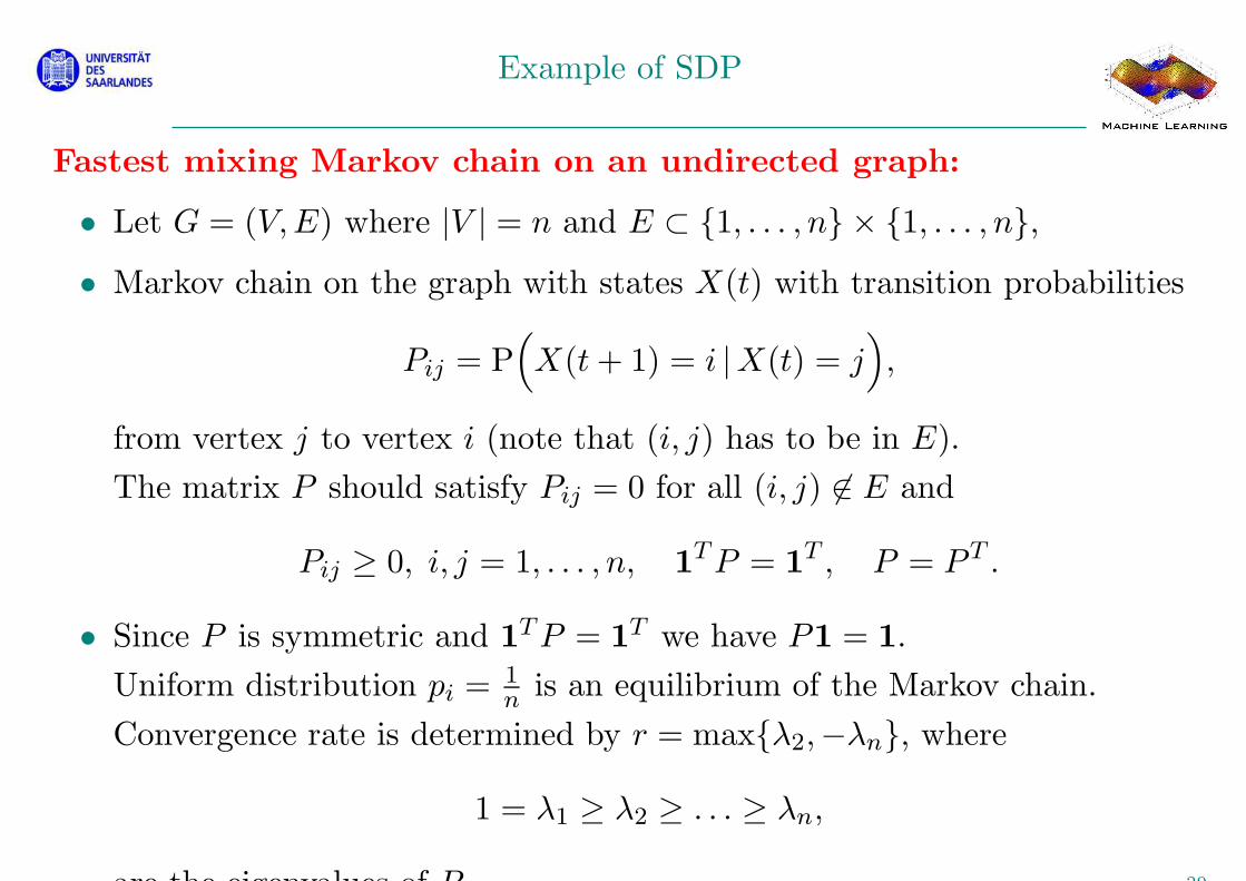
Example of SDP
Fastest mixing Markov chain on an undirected graph:
• Let G = (V,E) where |V | = n and E ⊂ {1, . . . , n} × {1, . . . , n},
• Markov chain on the graph with states X(t) with transition probabilities
Pij = P(
X(t + 1) = i |X(t) = j)
,
from vertex j to vertex i (note that (i, j) has to be in E).
The matrix P should satisfy Pij = 0 for all (i, j) 6∈ E and
Pij ≥ 0, i, j = 1, . . . , n, 1T P = 1T , P = P T .
• Since P is symmetric and 1T P = 1T we have P1 = 1.
Uniform distribution pi = 1
nis an equilibrium of the Markov chain.
Convergence rate is determined by r = max{λ2,−λn}, where
1 = λ1 ≥ λ2 ≥ . . . ≥ λn,
are the eigenvalues of P . 29
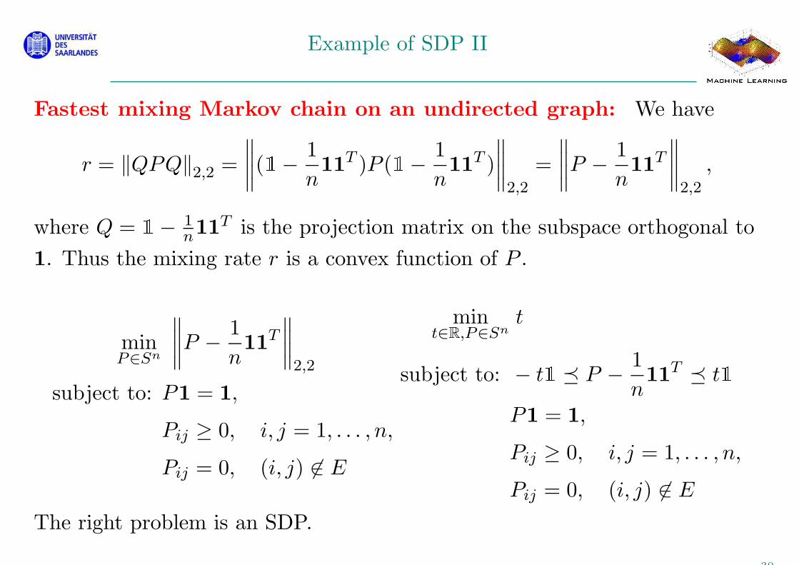
Example of SDP II
Fastest mixing Markov chain on an undirected graph: We have
r = ‖QPQ‖2,2 =
∥
∥
∥
∥
(1−1
n11T )P (1−
1
n11T )
∥
∥
∥
∥
2,2
=
∥
∥
∥
∥
P −1
n11T
∥
∥
∥
∥
2,2
,
where Q = 1− 1
n11T is the projection matrix on the subspace orthogonal to
1. Thus the mixing rate r is a convex function of P .
minP∈Sn
∥
∥
∥
∥
P −1
n11T
∥
∥
∥
∥
2,2
subject to: P1 = 1,
Pij ≥ 0, i, j = 1, . . . , n,
Pij = 0, (i, j) 6∈ E
mint∈R,P∈Sn
t
subject to: − t1 � P −1
n11T � t1
P1 = 1,
Pij ≥ 0, i, j = 1, . . . , n,
Pij = 0, (i, j) 6∈ E
The right problem is an SDP.
30