Continuous-Time Regime Switching Models,Portfolio Optimization and Filter-Based Volatility
Jorn Sass
joint work with . . . , Elisabeth Leoff, Vikram Krishnamurthy
[email protected] of Kaiserslautern, Germany
Wien, March 6, 2015

Outline
Regime switching, portfolio optimization, filter-basedvolatility
Markov switching and hidden Markov models (MSMs and HMMs)
Partial information and filtering
Portfolio optimization
Continuous versus discrete time
HMMs with non-constant volatility
2 / 28

MSMs and HMMs
Markov switching and hidden Markov models (MSMs and HMMs)
3 / 28
MSMs and HMMs MSM
A continuous-time Markov switching model (MSM)
Observation process R = (Rt)t∈[0,T ], e.g. stock returns,
Rt =
∫ t
0
µs ds +
∫ t
0
σs dWs
Drift µt = b⊤Yt =∑
biYit , b ∈ Rd , and volatility σt = a⊤Yt , a ∈ Rd
>0
Y = (Yt)t∈[0,T ) continuous-time Markov chain with states {e1, . . . , ed}
W standard Brownian motion, independent of Y
Jumps are governed by rate matrix Q ∈ Rd×d
Diagonal: Exponential rate of leaving state ek ,
λk = −Qkk =∑
l 6=k
Qkl < ∞
Conditional transition probability:
P(Yt = el |Yt− = ek ,Yt 6= Yt−) = Qkl/λk
4 / 28

MSMs and HMMs MSM
Example: Simulated data
0 0.2 0.4 0.6 0.8 11
2
3State process
0 0.2 0.4 0.6 0.8 1−2
02
Drift process
0 0.2 0.4 0.6 0.8 10.1
0.15
0.2
Volatility process
0 0.2 0.4 0.6 0.8 1−0.03
0
0.03 Daily stock returns
0 0.2 0.4 0.6 0.8 10.8
1
1.2Price process
∆t = 1250 , b
⊤ = (3, 0,−2), a⊤ = (0.20, 0.12, 0.15), Q =
(−70 40 3020 −40 2030 50 −80
)
5 / 28
MSMs and HMMs Multivariate stock index data
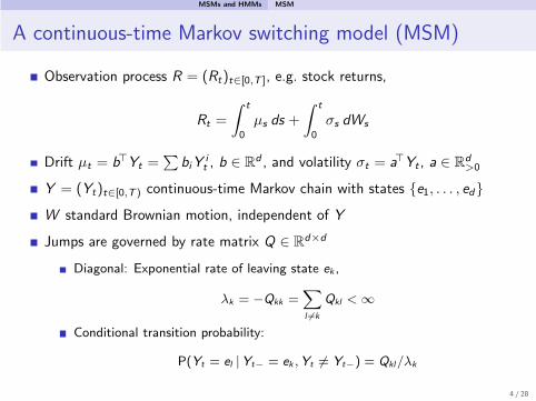
Exmple: Daily returns of stock indices
−0.2
−0.1
0
0.1
0.2
−0.2
−0.1
0
0.1
0.2
−0.2
−0.1
0
0.1
0.2
01/98 01/99 01/00 01/01 01/02 01/03 01/04 01/05 01/06 01/07 01/08−0.2
−0.1
0
0.1
0.2
Figure: Daily returns over 10 years for S&P 500, IPC, MerVal, Bovespa
6 / 28

MSMs and HMMs Multivariate stock index data
Estimation of state probabilities
1998 1999 2000 2001 2002 2003 2004 2005 2006 2007 20080
0.5
1
1998 1999 2000 2001 2002 2003 2004 2005 2006 2007 20080
0.5
1
1998 1999 2000 2001 2002 2003 2004 2005 2006 2007 20080
0.5
1
1998 1999 2000 2001 2002 2003 2004 2005 2006 2007 20080
0.5
1
State probabilities for states 1 to 4
Estimation by MCMC methods in Hahn/Fruhwirth-Schnatter/S. (2010)7 / 28
MSMs and HMMs MSM and HMM
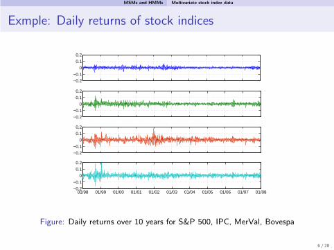
Properties, motivation of MSM, HMM
Properties, see Ryden/Terasvirta/Asbrink (1998), Timmermann (2000):
Wide ranges for skewness, kurtosis, tails; leverage and volatility clustering
Negative: No jumps, decay of autocorrelation of |∆R|, ∆R2 too fast
Interpretation:
State process models unobservable underlying economic variable
Rare jumps – structural breaks, frequent jumps – arrival of news
Many applications, e.g. in biophysics, finance, signal processing
MSM and HMM: Since
[R]t =
∫ t
0
σ2s ds =
d∑
i=1
a2i
∫ t
0
1{Ys=ei}ds,
we distinguish
MSM if ai 6= aj for all i , j .
HMM if a1 = . . . = ad (hidden Markov model).
8 / 28

Partial information and filtering
Partial information and filtering
9 / 28
Partial information and filtering Information
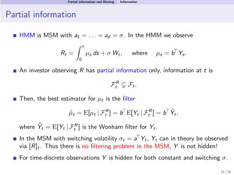
Partial information
HMM is MSM with a1 = . . . = ad = σ. In the HMM we observe
Rt =
∫ t
0
µs ds + σWt , where µs = b⊤Ys .
An investor observing R has partial information only, information at t is
FRt ( Ft .
Then, the best estimator for µt is the filter
µt = E[µt | FRt ] = b⊤E[Yt | F
Rt ] = b⊤Yt ,
where Yt = E[Yt | FRt ] is the Wonham filter for Yt .
In the MSM with switching volatility σt = a⊤Yt , Yt can in theory be observedvia [R]t . Thus there is no filtering problem in the MSM, Y is not hidden!
For time-discrete observations Y is hidden for both constant and switching σ.
10 / 28
Partial information and filtering Filtering in the HMM
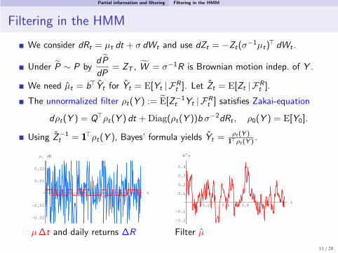
Filtering in the HMM
We consider dRt = µt dt + σ dWt and use dZt = −Zt(σ−1µt)
⊤ dWt .
Under P ∼ P bydP
dP= ZT , W = σ−1R is Brownian motion indep. of Y .
We need µt = b⊤Yt for Yt = E[Yt | FRt ]. Let Zt = E[Zt | F
Rt ].
The unnormalized filter ρt(Y ) := E[Z−1t Yt | F
Rt ] satisfies Zakai-equation
dρt(Y ) = Q⊤ρt(Y ) dt +Diag(ρt(Y ))b σ−2dRt , ρ0(Y ) = E[Y0].
Using Z−1t = 1⊤ρt(Y ), Bayes’ formula yields Yt =
ρt (Y )1⊤ρt(Y )
.
0.2 0.4 0.6 0.8 1t
-0.02
-0.01
0.01
0.02
Μ, dR
0.2 0.4 0.6 0.8 1t
-0.2
-0.1
0.1
0.2
0.3
0.4
bTΗ
µ∆t and daily returns ∆R Filter µ
11 / 28

Portfolio optmization
Portfolio optimization
12 / 28
Portfolio optmization Trading
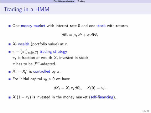
Trading in a HMM
One money market with interest rate 0 and one stock with returns
dRt = µt dt + σ dWt
Xt wealth (portfolio value) at t.
π = (πt)t∈[0,T ] trading strategy
πt is fraction of wealth Xt invested in stock.
π has to be FR -adapted.
Xt = Xπt is controlled by π.
For initial capital x0 > 0 we have
dXt = Xt πtdRt , X (0) = x0.
Xt(1− πt) is invested in the money market (self-financing).
13 / 28
Portfolio optmization Utility maximization problem
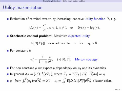
Utility maximization
Evaluation of terminal wealth by increasing, concave utility function U, e.g.
Uα(x) =xα
α, α < 1, α 6= 1 or U0(x) = log(x).
Stochastic control problem: Maximize expected utility
E[U(XπT )] over admissible π for x0 > 0.
For constant µ
π∗t =
1
1− α
µ
σ2, t ∈ [0,T ], Merton strategy.
For non-constant µ we expect a dependency on µt and its dynamics.
In general X ∗T = (U ′)−1(yZT ), where ZT = E[ZT | FR
T ], E[X∗T ] = x0.
π∗ from∫ T
0(π∗
t )σdWt = X ∗T − x0 =
∫ T
0E[DtX
∗T |F
Rt ]dWt if latter exists.
14 / 28

Portfolio optmization Optimal strategies
Optimal trading strategies
In the HMM (S./Haussmann 2004)
π∗t =
1
(1− α)E[Z
α
α−1
t,T | ρt
]{σ−2b⊤YtE
[Z
2α−1α−1
t,T | ρt
]
+ σ−1E[Z
2α−1α−1
t,T
∫ T
t
(Dtρt,s)bσ−2dRs
∣∣∣ ρt]}
.
For U = log this becomes π∗t = σ−2µt = σ−2b⊤Yt .
In the MSM (Bauerle/Rieder 2004) for
π∗t =
1
1− α
b⊤Yt
(a⊤Yt)2.
For U = log this becomes π∗t = σ−2
t µt = (a⊤Yt)−2b⊤Yt .
15 / 28

Continuous versus discrete time
Continuous versus discrete time
16 / 28
Continuous versus discrete time Continuous-time optimal strategies
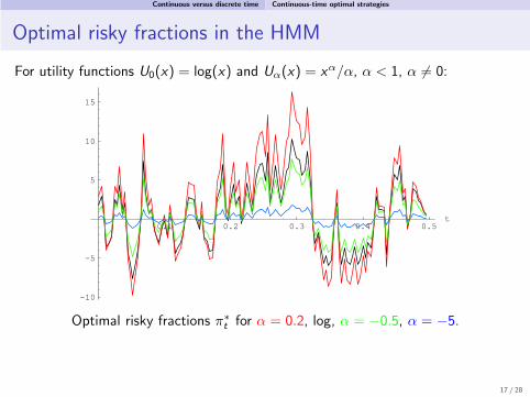
Optimal risky fractions in the HMM
For utility functions U0(x) = log(x) and Uα(x) = xα/α, α < 1, α 6= 0:
0.1 0.2 0.3 0.4 0.5t
-10
-5
5
10
15
Optimal risky fractions π∗t for α = 0.2, log, α = −0.5, α = −5.
17 / 28

Continuous versus discrete time Application of optimal strategies and discretization
Implementation of optimal strategies
For maximizing E [log(XπT )], the optimal risky fraction is π∗
t = σ−2 µt .
Constrained strategy: No short selling, no borrowing: Cut off π∗ at 0, 1.
Average log-utilities (500 simulations) for different trading frequencies:
strategy 10/day 5/day 4/day 2/day daily every 2 days
constrained 0.261 0.256 0.246 0.230 0.192 0.165
for d = 2, σ = 0.4, b⊤ = (2.5,−1.5), Q12 = 60, Q21 = 40, i.e. E[µt ] = 0.1.
In discretized model same results as for constrained strategy.
Thus in the HMM, the discretized model is well approximated by thecontinuous time model with constraints (or with mild parameters).
Optimal constrained strategy in continuous-time MSM leads to optimalexpected utilities about 0.968 versus 0.192.
Thus, continuous-time MSM is poor approximation for discrete-time MSM.
18 / 28
Continuous versus discrete time Why MSM?
Reminder
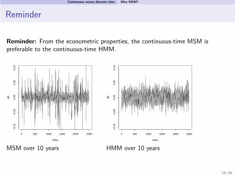
Reminder: From the econometric properties, the continuous-time MSM ispreferable to the continuous-time HMM.
0 500 1000 1500 2000 2500
−0.
10−
0.05
0.00
0.05
0.10
Index
dR
0 500 1000 1500 2000 2500
−0.
10−
0.05
0.00
0.05
0.10
Index
dR
MSM over 10 years HMM over 10 years
19 / 28
HMMs with non-constant volatility
HMMs with non-constant volatility
20 / 28
HMMs with non-constant volatility Filter based volatility
MSM versus HMM with non-constant volatility
The continuous-time MSM is a poor approximation for the discrete timemodel in view of portfolio optimization.
Idea: Consider a HMM with a non-constant volatility model,
dRt = b⊤Yt + σt dWt ,
where σt = f (Yt), as approximation for the MSM.
This yields consistent continuous-time approximations, since
For non-constant σt filters can be computed (Haussmann/S. 2004).
For non-constant σt , optimal strategy π∗t can be computed as above.
It then has an additional term due to the dynamics of σt .
The dependency can be modelled such that f (Yt) = a⊤Yt .
Any dynamic volatility model w.r.t. W can be used.
21 / 28

HMMs with non-constant volatility Filter based volatility
Daily returns and volatility process
0 50 100 150 200 250
−0.0
50.
000.
05
Index
dR
0 50 100 150 200 250
−0.0
50.
000.
05
Index
dR
MSM HMM with constant σ
0 50 100 150 200 250
−0.0
50.
000.
05
Index
dR
0 50 100 150 200 250
−0.0
50.
000.
05
Index
dR
HMM with σt linear in Yt HMM with σt quadratic in Yt
22 / 28

HMMs with non-constant volatility Filter based volatility
HMM with non-constant volatility closest to MSM
Consider for FR adapted (σt)t∈[0,T ]
dRt = b⊤Ytdt + a⊤YtdWt and dRHt = b⊤Ytdt + σtdWt
The mean squared distance of the return processes is
MSE(R ,RH) =1
TE
[∫ T
0
(Rt − RHt )2dt
].
We have
MSE(R,RH) =1
T
∫ T
0
∫ t
0
E[(a⊤Ys − σs)
2]ds dt.
This is minimized by
σt = E[a⊤Yt | F
Rt
]= a⊤Yt .
In this sense, the HMM with σt = a⊤Yt is the HMM closest to MSM.
23 / 28

HMMs with non-constant volatility Filter based volatility
Comparison of some econometric properties
Square distance of HMM with σt andMSM with volatility a⊤Yt is minimizedby
σt = f (Yt) = a⊤Yt .−0.05 −0.04 −0.03 −0.02 −0.01 0 0.01 0.02 0.03 0.04 0.05
0
5
10
15
20
25
30
35
40
45
50
Histogram SV − identical bins
−0.05 −0.04 −0.03 −0.02 −0.01 0 0.01 0.02 0.03 0.04 0.050
5
10
15
20
25
30
35
40
45
50
Histogram MSM − identical bins
MSM vs. HMM with σt
2 4 6 8 10 12 14 16 18 200
0.05
0.1
0.15
0.2
0.25
0.3
0.35Estimated absolute ACF
SVMSM
Estimated absolute ACF
2 4 6 8 10 12 14 16 18 200
0.05
0.1
0.15
0.2
0.25
0.3
0.35
0.4
0.45
0.5Estimated square ACF
SVMSM
Estimated square ACF24 / 28

Conclusion
Conclusion
25 / 28

Conclusion Extensions
Model choice, risk constraints and expert opinions
Model choice: Wrong model might work better in view of estimation errors:In a Black Scholes model with µ ∈ [a, b] using an HMM with states a, boutperforms using constant but estimated µ.
Suitable bounds a, b can be obtained by semi-dynamic risk constraints, seeCuoco/He/Issaenko 2007, Putschogl/S. 2011.
Static risk constraints on the distribution of the terminal wealth can beincluded. E.g., for ε = 0.01 and binding constraint E[ZT (X
∗T − q)−] = ε:
0.5 1.0 1.5 2.0
01
23
4
X*(T)
density
Pdf of X ∗T without and with risk
constraint q = 0.9 (atom 2.94%)
0.5 1.0 1.5 2.0
01
23
4X*(T)
density
Pdf of X ∗T without and with risk
constraint q = 1.0 (atom 40.21%)
See Basak/Shapiro 2001, Gabih/S./Wunderlich 2009, S./Wunderlich 2010
Expert opinions: Frey/Gabih/Wunderlich 2012/14, G./Kondakji/S./W. 201426 / 28

Conclusion Summary
Summary and related models
Differences of HMM and MSM:
In HMM: Full and partial information. Partial information with constraints onstrategy is consistent approximation for discrete-time model.
In MSM: In continuous time only full information. No good approximation fordiscretized model.
But MSM has better econometric properties
HMM with non-constant volatility might be a good compromise.
Non-constant volatility can be chosen to minimize distance HMM–MSM.
Filtering, estimation and optimization work for n stocks.
Similar questions regarding continuous versus discrete-time model for modelswith Levy noise with compound Poisson part.
Other models for µ which allow for explicit filtering and computation ofoptimal strategies:
µ as an Ornstein-Uhlenbeck process; leads to Kalman filtering (Lakner 1998).
27 / 28
Conclusion References
Further reading
S./Haussmann (2004) Optimizing the terminal wealth under partial information: The drift process as acontinuous time Markov chain, Finance and Stochastics 8, 553-577.
Haussmann/S. (2004) Optimal terminal wealth under partial information for HMM stock returns. In: G.Yin and Q. Zhang (eds.): Mathematics of Finance: Proceedings of an AMS-IMS-SIAM SummerConference June 22-26, 2003, Utah, AMS Contemporary Mathematics 351, 171–185.
Hahn/Putschogl/S. (2007) Portfolio optimization with non-constant volatility and partial information,Brazilian Journal of Probability and Statistics 21, 27–61.
Elliott/Krishnamurthy/S. (2008) Moment based regression algorithm for drift and volatility estimationin continuous time Markov switching models, Econometrics Journal, 11, 244–270.
Gabih/S./Wunderlich (2009): Utility maximization under bounded expected loss, Stochastic Models 25,375–407.
S./Wunderlich (2010): Optimal portfolio policies under bounded expected loss and partial information,Mathematical Methods of Operations Research 72, 25–61.
Hahn/Fruhwirth-Schnatter/S. (2010) Markov chain Monte Carlo methods for parameter estimation inmultidimensional continuous time Markov switching models, Journal of Financial Econometrics 8,88–121.
Putschogl/S. (2011): Optimal investment under dynamic risk constraints and partial information,Quantitative Finance 11, 1547–1564.
Gabih/Kondakji/S./Wunderlich (2014): Expert opinions and logarithmic utility maximization in amarket with Gaussian drift, Communications on Stochastic Analysis 8, 27–47.
28 / 28