Conjunctive use modeling for multicrop irrigation
S. Vedulaa, P.P. Mujumdara,�, G. Chandra Sekharb
aDepartment of Civil Engineering, Indian Institute of Science (IISc), Bangalore 560 012, IndiabNational Remote Sensing Agency, Hyderabad 500 037, India
Accepted 26 October 2004
Abstract
A mathematical model is developed to arrive at an optimal conjunctive use policy for irrigation of
multiple crops in a reservoir-canal–aquifer system. The integration of the reservoir operation for canal
release, ground water pumping and crop water allocations during different periods of crop season
(intraseasonal periods) is achieved through the objective of maximizing the sum of relative yields of
crops over a year considering three sets of constraints: mass balance at the reservoir, soil moisture
balance for individual crops, and governing equations for ground water flow. The conjunctive use
model is formulated with these constraints linked together by appropriate additional constraints as a
deterministic linear programming model. A two-dimensional isotropic, homogeneous unconfined
aquifer is considered for modeling. The aquifer response is modeled through the use of a finite element
ground water model. A conjunctive use policy is defined by specifying the ratio of the annual allocation
of surface water to that of ground water pumping at the crop level for the entire irrigated area. A
conjunctive use policy is termed stable when the policy results in a negligible change in the ground
water storage over a normal year. The applicability of the model is demonstrated through a case study
of an existing reservoir command area in Chitradurga district, Karnataka State, India.
# 2004 Elsevier B.V. All rights reserved.
Keywords: Conjunctive use model; Reservoir–aquifer system; Multicrop irrigation; Stable operating policy
1. Introduction
There is very little work done in the past to integrate the decision making with respect to
the release at the reservoir, the pumping from the aquifer and water allocation to individual
www.elsevier.com/locate/agwat
Agricultural Water Management 73 (2005) 193–221
� Corresponding author. Tel.: +91 803 600290.
E-mail address: [email protected] (P.P. Mujumdar).
0378-3774/$ – see front matter # 2004 Elsevier B.V. All rights reserved.
doi:10.1016/j.agwat.2004.10.014

S. Vedula et al. / Agricultural Water Management 73 (2005) 193–221194
Nomenclature
al;m element in ½A�ac
t ratio of actual to potential evapotranspiration from crop c in period t
(stable policy parameter)
½A�, ½B� global coefficient matrices
Aa water spread area per unit active storage volume above A0
A0 water spread area corresponding to the dead storage volume
Ae area of element e
availt availability of water for release from the reservoir for each period t
AET actual evapotranspiration
AETct actual evapotranspiration for crop c in time period t
Areac area of crop c
B (i) boundary of the study area (B ¼ Bh þ B0 þ Bq), (ii) base flow
accumulation in the study area
Bh part of boundary over which water levels are specified as boundary
condition
Bq part of boundary over which specified boundary condition applies
B0 part of boundary over which zero flow condition applies
c crop index
Canalrechet recharge from canal seepage for element e in time period t, in m
Dct average root depth during period t for crop c
DPct deep percolation during period t from the root zone of crop c
ET0 reference evapotranspiration
Evapt estimated evaporation loss in period t
g growth stage index
gll ground level at node l
G arbitrarily big number
h ground water level
½h� vector of ground water levels at time period ðt þ 1Þh0m ground water level at node m at time t
½h0� vector of ground water levels at time t
htl ground water level at node l at time ðt þ 1Þ
kt crop factor for growth stage to which the period t belongs
kyg yield factor for the growth stage g
kycg yield factor for the growth stage g of crop c
l node index
M number of nodes
Ne1;Ne
m element shape functions
NC number of crops
NGS number of growth stages
O net outflow from the study area
OVFt overflow from the reservoir during period t
P net ground water pumping from the study area

S. Vedula et al. / Agricultural Water Management 73 (2005) 193–221 195
PET potential evapotranspiration
PETct potential evapotranspiration for crop c in period t
q outflow rate per unit length
QP pumping rate per unit area
QR recharge rate per unit area
Qt reservoir inflow during period t
QePt
ground water pumping rate from element e during period t
QeRt
ground water recharge rate from element e during period t
rt ratio of surface water allocated to total water allocated at crop level
RB boundary residue
Rc recharge from canal seepage in the study area
RD domain residue
Ri recharge from irrigated area in the study area
Rr recharge from rainfall in the study area
Rt reservoir release for the period t
Raint rainfall in period t
Relt reservoir release made in period t
DS net change in ground water storage over the study area
Smax reservoir live storage capacity
St reservoir storage at the beginning of period t
Sy specific yield
SAt actual reservoir storage at the beginning of the period t
SMmax maximum available soil moisture in the root zone
SMcmax maximum available soil moisture in the root zone for crop c
SMct available soil moisture in the root zone for crop c at the beginning
of period t
t time period index
Dt time step
T transmissivity
Wl, W̄l weighting functions
x; y Cartesian coordinates
xct surface water allocation to crop c in period t
xgct ground water allocation to crop c in period t
y actual yield of crop
ymax maximum yield of crop
Greek letters
d rainfall recharge coefficient
h conveyance efficiency
lt (0 or 1) integer variable
crops in multicrop irrigation in reservoir canal command areas. The present study is an
investigation aimed in this direction. The study attempts to model conjunctive use and
develop a stable operating policy for optimal allocation of surface and ground waters for
irrigating multiple crops in a canal command area.
1.1. Conjunctive use models
Based on the technique used, conjunctive use models developed earlier may be
classified as simulation models, dynamic programming models, linear programming
models, hierarchical optimization models, nonlinear programming models, and others.
Simulation approaches provided a framework for conceptualizing, analyzing and
evaluating stream–aquifer systems. Since the governing partial differential equations for
complex heterogeneous ground water and stream–aquifer systems are not amenable to
closed form analytical solution, various numerical models using finite difference or finite
element methods have been used for solution (Chun et al., 1964; Bredehoeft and Young,
1970, 1983; O’Mara and Duloy, 1984; Latif and James, 1991; Chaves-Morales et al., 1992).
Dynamic programming (DP) has been used because of its advantages in modeling
sequential decision making processes, and applicability to nonlinear systems, ability to
incorporate stochasticity of hydrologic processes and obtain global optimality even for
complex policies (Buras, 1963; Aron, 1969; Cochran and Butcher, 1970; Coskunoglu and
Shetty, 1981; Onta et al., 1991; Provencher and Burt, 1994). However, the ‘‘curse of
dimensionality’’ seems to be the major reason for limited use of DP in conjunctive use
studies. These studies considered physical system as lumped. Jones et al. (1987) used a
DDP algorithm to reduce computational burden for unsteady, nonlinear (unconfined),
ground water system management problems.
Linear Programming (LP) has been the most widely used optimization technique in
conjunctive modeling. Rogers and Smith (1970) formulated a linear programming model
incorporating ground water budget concept. The groundwater response was considered as
lumped. Nieswand and Granstrom (1971) developed a set of chance constrained linear
programming models for the conjunctive use of surface waters and ground waters for the
Mullica River basin in New Jersey. Lakshminarayana and Rajagopalan (1977) studied the
problem of optimal cropping pattern and water releases from canals and tubewells in the
Bari Doab basin, India, using a linear programming model. The model is a deterministic
model and the dynamic response of the ground water aquifer was not considered.
Hierarchical optimization models were developed by Maddock (1972, 1973); Haimes
and Dreizin (1977); Morel-Seytoux (1975); Yu and Haimes (1974); Dreizin and Haimes
(1977), and Paudyal and Gupta (1990).
Belaineh et al. (1999) present a simulation/optimization model that integrates linear
reservoir decision rules, detailed simulations of stream/aquifer system flows, conjunctive
use of surface and ground water, and delivery via branching canals to water users. State
variables, including aquifer hydraulic head, streamflow, and surface water/aquifer
interflow, are represented through discretized convolution integrals and influence
coefficients. Reservoir storage and branching canal flows and interflows are represented
using embedded continuity equations. Results of application indicate that the more detail
used to represent the physical system, the better the conjunctive management. Azaiez and
S. Vedula et al. / Agricultural Water Management 73 (2005) 193–221196

Hariga (2001) developed a model for a multi-reservoir system, where the inflow to the main
reservoir and the demand for irrigation water at local areas are stochastic. High penalty
costs for pumping groundwater are imposed to reduce the risk of total depletion of the
aquifer as well as quality degradation and seawater intrusion. The problem is analyzed for a
single period with a single decision-maker approach. Deficit irrigation is allowed in
maximizing expected total profit for the entire region. A nonlinear stochastic problem with
linear constraints is formulated and an iterative procedure that generates an optimal
operating policy is proposed. Model application is illustrated with a hypothetical example.
Barlow et al. (2003) developed conjunctive-management models that couple numerical
simulation with linear optimization to evaluate trade-offs between groundwater
withdrawals and streamflow depletions for alluvial-valley stream–aquifer systems
representative of those of the northeastern United States. The model developed for a
hypothetical stream–aquifer system was used to assess the effect of interannual hydrologic
variability on minimum monthly streamflow requirements. The conjunctive-management
model was applied to a stream–aquifer system of central Rhode Island.
Rao et al. (2004) developed a regional conjunctive use model for a near-real deltaic aquifer
system, irrigated from a diversion system, with some reference to hydrogeoclimatic
conditions prevalent in the east coastal deltas of India. The combined simulation-
optimization model proposed in this study is solved as a nonlinear, nonconvex combinatorial
problem using a simulated annealing algorithm and an existing sharp interface model. The
computational burden is managed within practical time frames by replacing the flow
simulator with artificial neural networks and using efficient algorithmic guidance.
Marino (2001) discussed simulation and optimization models and decision-support
tools that have proven to be valuable in the planning and management of regional water
supplies. Also conjunctive water management issues in California as well as water
management approaches for effectively dealing with climate change are discussed.
Despite the fact that most conjunctive use management problems are nonlinear in
nature, application of nonlinear programming (NLP) has been rather limited. This may be
because of the complexity and the slow rate of convergence of the NLP algorithms,
difficulty in considering stochasticity and possibility of getting a local instead of global
optimal solution (Yeh, 1992). Willis et al. (1989); Matsukawa et al. (1992) are among those
who used nonlinear programming for conjunctive use modeling.
A study of the existing literature shows that there is no single comprehensive model
developed for irrigation of multiple crops in which reservoir operation and irrigation
allocation decisions at field level are integrated, and in which a conjunctive use policy for
the irrigated area, apportioning the surface and ground water components, taking into
account the distributed parameter characteristics of the aquifer and the soil moisture
dynamics at the crop level, is embedded. The present study is an attempt in this direction
and in the identification of a stable conjunctive use policy for canal command areas.
1.2. Objectives of the study
The specific objectives of the present study are: (1) to develop a mathematical
programming model to determine a stable conjunctive use policy for irrigation in a
reservoir–aquifer system for multiple crops in a reservoir canal command area, for a
S. Vedula et al. / Agricultural Water Management 73 (2005) 193–221 197

normal year, (2) to extract the optimal temporal crop water allocation pattern from the
identified stable policy for application to a given year, using simulation, and (3) to apply the
model, derive a stable conjunctive policy for an existing canal command area, and apply
the policy over a period of time to examine the aquifer response (storage) for stability.
2. Model formulation
An overview of the overall model is presented first. The model formulation with all its
associated components is presented next. Following this, the concept of a conjunctive use
policy and of a stable policy as used in the present study are discussed. The methodology of
arriving at a stable conjunctive use policy and its application to an existing reservoir canal
command area are presented next.
2.1. Model overview
A schematic diagram of the conjunctive use system is presented in Fig. 1. The system is
characterized by three main components: the reservoir, the irrigated area and the underlying
aquifer with the associated dynamic relationships defining the interactions among them. A
mathematical formulation is developed to arrive at an optimal conjunctive use policy of
ground and surface waters for the irrigation of multiple crops in an irrigated area under the
command of reservoir. The model considers varying soil moisture conditions and soil types
and takes into account the dynamic response of the aquifer in the reservoir command area to
surface application, pumping and recharge. The integration of decision making in reservoir
operation, ground water pumping and crop water allocations during the different periods of
S. Vedula et al. / Agricultural Water Management 73 (2005) 193–221198
Fig. 1. Schematic diagram of the conjunctive use system.

crop season (intraseasonal periods) is achieved through optimization with the objective of
maximizing the sum of relative yields of crops over a year, and considering three sets of
constraints: mass balance at the reservoir, soil moisture continuity for individual crops, and
governing equations for ground water flow. These sets of constraints are linked together
appropriately by additional constraints. The reservoir release and the ground water are
optimally allocated to achieve the maximum annual relative yield of crops.
A two-dimensional, isotropic, homogeneous unconfined aquifer is considered. The
aquifer response is modeled through the use of a finite element ground water model. The study
area is discretized into a number of elements for this purpose. A given crop is assumed to grow
in integral number of elements. The soil moisture continuity is considered for each cropped
area which consists of several elements. Thus, the variables in the soil moisture balance
equation for a given period will assume the same values over all the elements of a given
cropped area. The governing partial differential equations representing the ground water flow
are transformed into linear algebraic equations using Galarkin method of weighted residuals.
These equations are written for each node, and are embedded into the optimization model as
constraints. The aquifer parameters (specific yield and transmissivity) are assumed to be
known. A study area larger than the canal command area is considered such that the boundary
conditions along the boundary of the study area can be assumed to be unaffected by the
irrigation operation within the command area. The boundary conditions specified correspond
to those of a normal year. To specify the initial conditions at each node in the study area,
ground water contours are drawn from the data of observation wells in and around the study
area, and the initial conditions are specified accordingly. The recharge to the aquifer from an
element consists of the recharge due to rainfall, canal seepage and the deep percolation from
the root zone of the crop grown in the element. Thewaterlogging condition in the study area is
avoided by imposing an upper bound on the ground water level at each node.
The objective of maximizing the sum of relative crop yields is expressed using an additive
crop production function. The conjunctive use model is formulated as a deterministic linear
programming model. Reservoir inflow and rainfall in the canal command area in each time
period are assumed deterministic. The decision variables in the model for each intraseasonal
period are: reservoir release, reservoir storage, ground water pumping required for each crop,
surface water allocation for each crop, deep percolation, if any, from the root zone of the crop,
actual evapotranspiration of each crop, ground water head at each node in the study area and
the soil moisture at the beginning of the period for each crop.
A conjunctive use policy is defined by specifying the ratio of the annual allocation of
surface water to that of ground water pumping at the crop level for entire irrigated area. A
given policy is characterized by the ratio of annual irrigation water application at crop level
from surface to ground sources. For example, a 70:30 policy refers to one in which 70% of
the annual irrigation application, at the crop level, comes from surface source and 30%
from ground water pumping. A policy is termed stable when it results in negligible change
in the ground water storage over a normal year.
The conjunctive use model is run for different pre-determined ratios of annual surface
and ground water applications at the crop level (i.e. for different conjunctive use policies).
Ground water balance components over the entire study area are computed for each of
these runs, and an examination of annual ground water balance is made in each case. The
policy for which the annual change in ground water storage is negligible for a normal year
S. Vedula et al. / Agricultural Water Management 73 (2005) 193–221 199

is considered as the ‘‘stable policy’’. Optimal temporal allocation patterns are derived from
the results of the stable policy for the specific case considered and applied to examine the
aquifer storage response over years for stability. The derived stable conjunctive use policy
aids in planning the total crop water allocation for irrigation in the study area.
2.2. Ground water model
The purpose of this model is to incorporate the dynamic response of the aquifer to
ground water extraction for irrigation and ground water recharge due to deep percolation
from irrigated area, rainfall and canal seepage. The ground water response is modeled
using the finite element method. The partial differential equations representing the ground
water flow are transformed into linear algebraic equations using the finite element method
in space and finite differencing of time. These equations, which represent the response of
the aquifer to the external stresses of ground water extraction and recharge along with the
bounds on the ground water levels, are embedded into the linear programming (LP) model
as constraints. The ground water model is discussed in detail in the following sections.
2.2.1. Governing equations
The following assumptions are made in the ground water model:
1. The flow in the aquifer is approximated as a two dimensional flow.
2. Darcy’s law (head loss varying linearly with the apparent velocity) and Dupuit’s
assumption (negligible vertical flow) are applicable.
3. The aquifer is unconfined, homogeneous, isotropic and bounded at the bottom by an
impervious layer.
4. The saturated thickness of the aquifer is always large compared to the drawdown; thus
the aquifer transmissivity is independent of the head.
The governing equation for a two-dimensional, unsteady flow in an isotropic, homo-
geneous, unconfined aquifer is given by Yeh (1992)
@
@xT@h
@x
� �þ @
@yT@h
@y
� �¼ Sy
@h
@tþQP � QR (1)
where h is the ground water level in m; T the transmissivity in m2=day; Sy the specific yield;
QP the pumping rate per unit area in m3=ðday m2Þ; QR the recharge rate per unit area in
m3=ðday m2Þ; x and y are the Cartesian coordinates in plan, and t is the time in days.
2.2.2. Boundary conditions
The solution of Eq. (1) requires specification of initial and boundary conditions. A larger
study area is considered compared to the canal command area such that the boundary
conditions along the boundary of the study area can be assumed to be unaffected by the
irrigation operation within the command area. The initial conditions correspond to the
specification of water levels within the domain of the study area at the starting period. The
boundary conditions require specification of appropriate conditions at the external
boundaries such as the boundaries of the study area and internal boundaries such as rivers if
S. Vedula et al. / Agricultural Water Management 73 (2005) 193–221200
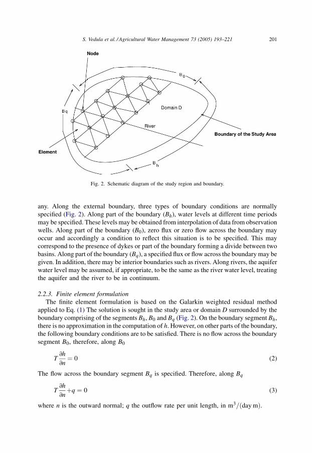
any. Along the external boundary, three types of boundary conditions are normally
specified (Fig. 2). Along part of the boundary (Bh), water levels at different time periods
may be specified. These levels may be obtained from interpolation of data from observation
wells. Along part of the boundary (B0), zero flux or zero flow across the boundary may
occur and accordingly a condition to reflect this situation is to be specified. This may
correspond to the presence of dykes or part of the boundary forming a divide between two
basins. Along part of the boundary (Bq), a specified flux or flow across the boundary may be
given. In addition, there may be interior boundaries such as rivers. Along rivers, the aquifer
water level may be assumed, if appropriate, to be the same as the river water level, treating
the aquifer and the river to be in continuum.
2.2.3. Finite element formulation
The finite element formulation is based on the Galarkin weighted residual method
applied to Eq. (1) The solution is sought in the study area or domain D surrounded by the
boundary comprising of the segments Bh, B0 and Bq (Fig. 2). On the boundary segment Bh,
there is no approximation in the computation of h. However, on other parts of the boundary,
the following boundary conditions are to be satisfied. There is no flow across the boundary
segment B0, therefore, along B0
T@h
@n¼ 0 (2)
The flow across the boundary segment Bq is specified. Therefore, along Bq
T@h
@nþq ¼ 0 (3)
where n is the outward normal; q the outflow rate per unit length, in m3=ðday mÞ.
S. Vedula et al. / Agricultural Water Management 73 (2005) 193–221 201
Fig. 2. Schematic diagram of the study region and boundary.

The weighted residual equation, incorporating the domain and boundary residuals, may
be written asZD
WlRD dx dy þZ
B0
W̄lRB dB þZ
Bq
W̄lRB dB ¼ 0 (4)
where Wl and W̄l are the weighting functions, being functions of x and y.
The domain residue RD and the boundary residue RB are given by
RD ¼ @
@xT@h
@x
� �þ @
@yT@h
@y
� �� Sy
@h
@t�QP þ QR (5)
Along B0 : RB ¼ T@h
@n(6)
Along Bq : RB ¼ T@h
@nþq (7)
where h is the approximate solution for water level as obtained from the finite element
model.
The finite element approximation for h is given by
hðx; y; tÞ ¼XMm¼1
hmðtÞNmðx; yÞ (8)
where M is the total number of nodes in the domain; hm the water level at node m at time
ðt þ 1Þ; Nmðx; yÞ is the global shape function.
Eq. (4) can be written for M independent weighting functions Wl and W̄l (l ¼ 1 to M)
providing M equations for the M nodal values of hm at time (t þ 1). The set of equations can
be written in matrix notation as
½A�½h� ¼ ½B�½h0� þ ½F� (9)
where ½h�T ¼ ðht1; ht
2; . . . ; htMÞ is the vector of ground water heads at time t þ 1, ½h0�T ¼
ðht�11 ; ht�1
2 ; . . . ; ht�1M Þ is the vector of ground water heads at time t, T used as a superscript
on ½h� or ½h0� denotes its transpose, ½A� and ½B� are the global coefficient matrices and ½F� is a
vector.
These equations lead to a set of linear equations which are embedded as constraints
in the LP model subsequently. An upper bound is imposed on the ground water level.
Thus
htl ht
l;max 8 l; t (10)
where htl;max is the specified upper limit on the ground water level at node l in time
period t.
In the finite element procedure, the terms in the matrices ½A�; ½B� and ½F� in Eq. (9), are
assembled elementwise, using integration over the element domains and using element
shape functions. The element contributions are assembled to construct the global matrix
terms and the right side of Eq. (9) along with the upper bound on the ground water level
given by Eq. (10) are embedded into the LP model as constraints. The recharge to the
aquifer from rainfall, deep percolation from root zone of crops and canal seepage and the
ground water pumping, due to the application of ground water to the crop, are included in
S. Vedula et al. / Agricultural Water Management 73 (2005) 193–221202

the vector ½F�, which is computed for each element and assembled. The details of the finite
element model are presented by Chandra Sekhar (1998).
2.3. Crop yield optimization
Conjunctive use modeling for irrigation requires interfacing of reservoir operation, soil
moisture accounting and ground water balance. The first two aspects were dealt with in the
earlier studies of Vedula and Mujumdar (1992); Vedula and Nagesh Kumar (1996). Ground
water issues were not addressed in these, as no conjunctive use was contemplated. Much of
the formulation concerning reservoir operation and soil moisture balance in this paper
follows the concepts developed in these earlier studies. The formulation is extended in the
subsequent sections to take into account ground water balance and its integration into an
overall conjunctive use model.
The following additive type of production function is considered. It expresses the
relative yield of a crop as a function of deficits suffered in the individual growth stages
y
ymax¼ 1 �
XNGS
g¼1
kyg 1 � AET
PET
� �g
(11)
where y is the actual yield of the crop; ymax the maximum yield of the crop; g the growth
stage index; NGS the number of growth stages within the growing season of the crop; kyg
the yield response factor for the growth stage g; AET the actual and PET the potential
evapotranspiration.
The objective function used for optimally allocating water among the crops maximizes
an integral measure of relative crop yield in the area. For multiple crops, the annual sum of
the relative yields of all crops is taken as the integral measure to be maximized.
The objective function used for the overall conjunctive use model is
maximizeXNC
c¼1
1 �XNGS
g¼1
kycg 1 �
Xt 2 g
AETct
PETct
!" #(12)
where c is the crop index; g the growth stage of the crop; kycg the yield response factor for
the growth stage g of the crop c; NGS the number of growth stages of the crop, and NC the
number of crops.
The optimization is to maximize sum of relative yields of crops in the reservoir
command area. Optimization based on economic returns is not attempted. The model is
meant for application to small canal command areas, where irrigated agriculture is heavily
subsidized (such as in India) and the market prices do not reflect true marginal values to
society. Hence an objective function based on physical outputs is preferred.
The summation of AET and PET in Eq. (12) is for the periods t, within the growth stage
g, for the crop c. The objective function (Eq. (12)) implies minimization of the weighted
sum of the evapotranspiration deficits for the season.
The relative yield of a crop, y=ymax , in Eq. (11) would be equal to one if the volume of
water available for the season is greater than or equal to the total crop water requirement in
all the periods, thus permitting irrigation allocation to individual crops such that
AET ¼ PET. Irrigation allocation is made in the present study whenever the soil moisture
S. Vedula et al. / Agricultural Water Management 73 (2005) 193–221 203

in the root zone is above the permanent wilting point and below the field capacity. The
irrigation policy used is to irrigate such that the soil moisture in the root zone is brought to
the field capacity, to the extent possible depending on the water availability.
2.4. Soil moisture balance
The different elements considered in conceptualizing the soil moisture balance are
shown in Fig. 3. The inputs to the model for a given period are the rainfall, irrigation water
applied from surface and the aquifer, crop root depths at different times and the potential
evapotranspiration. The outputs are the actual evapotranspiration during the period, deep
percolation from the root zone during the period, if any, and the soil moisture in the root
zone at the end of the period.
At the beginning of the first period of the season the soil moisture is assumed to be at
field capacity, for all crops
SMc1 ¼ SMc
max 8 c (13)
where SMc1 is the available soil moisture(soil moisture above the permanent wilting point)
at the beginning of the first period for the crop c; SMcmax is the available soil moisture at the
field capacity for the crop c.
The soil moisture balance equation for a given crop c for any time period t is given by
SMctþ1Dc
tþ1 ¼SMct Dc
t þ xct þ xgc
t þ Raint � AETct
þ SMmax ðDctþ1 � Dc
t Þ � DPct 8 c; t (14)
where SMct is the available soil moisture at the beginning of the period t for the crop c; Dc
t
the average root depth during the period t for crop c; xct the irrigation allocation from
surface water to crop c in period t; xgct the irrigation allocation from ground water to crop c
in period t; Raint the rainfall in period t, assuming that all the rain would contribute to
enriching the soil moisture; AETct the actual evapotranspiration during period t for crop c;
DPct the deep percolation during the period t for crop c.
S. Vedula et al. / Agricultural Water Management 73 (2005) 193–221204
Fig. 3. Soil moisture transition.

The available soil moisture SMct and the maximum available soil moisture at field
capacity SMmax are in depth units per unit root depth, mm/cm, and all other terms are in
depth units, mm.
The available soil moisture in any time period t for crop c should not exceed the
maximum corresponding to the field capacity of the soil
SMct SMc
max 8 c; t (15)
Also,
AETct PETc
t 8 c; t (16)
where PETct is the potential evapotranspiration during period t for crop c.
A linear relationship between AET/PET and the soil moisture is maintained as per the
following constraint
AETct
SMct Dc
t þ xct þ xgc
t þ Raint
SMcmax Dc
t
� �PETc
t 8 c; t (17)
The following constraints are imposed to see that whenever the deep percolation exists, the
available soil moisture in the root zone of the crop at the end of the time period is at field
capacity. In other words DPt > 0 only when SMctþ1 ¼ SMc
max for any t. This is achieved by
introducing integer variables, l
DPct lc
t G 8 c; t (18)
lct
SMctþ1
SMcmax
8 c; t (19)
where lct is a binary (0 or 1) variable and G is an arbitrarily large number.
2.5. Reservoir water balance
The reservoir and storage constraints are written as in the earlier work of Vedula and
Mujumdar (1992).
2.6. Linking constraints
The dynamic relationships among the three main components of the conjunctive use
system – the reservoir, the aquifer and the irrigated area – are incorporated by imposing the
appropriate linkages as constraints in the model. The reservoir release is related to the
surface water allocations to the crops. The ground water pumping is related to the ground
water allocation to the crop grown in the element. The conveyance loss in canals is assumed
as a fraction of the release from the reservoir. The entire amount of canal seepage is
assumed to contribute to the ground water recharge, and is assumed distributed uniformly
among the elements through which the canal is running.
S. Vedula et al. / Agricultural Water Management 73 (2005) 193–221 205
The release from the reservoir in a given period after losses should equal to the sum of
the irrigation allocations from the surface reservoir to all crops in the period
hRt ¼XNC
c¼1
xct Areac 8 t (20)
where h is the conveyance efficiency factor; Rt the reservoir release in period t, in Mm3; xct
the irrigation allocation from surface water to crop c in period t, in mm; Areac the area of
the crop c, in km2.
The study area is discretized into a number of elements. The soil moisture continuity
is considered for each cropped area which consists of several elements. Thus, the
variables in the soil moisture balance equation for a given period will assume the same
values over all the elements of a given cropped area. The recharge to the aquifer is the
sum of the contributions from the rainfall, the deep percolation and the canal seepage.
Some elements fall into the category of nonirrigated area. For those elements, the
recharge due to rainfall is assumed as a known fraction of the rainfall occurring in the
element in a given period t. For the elements over the irrigated area, the recharge will be
accounted in the soil moisture balance equation through the deep percolation term
(Eq. (14)).
The recharge to the aquifer from the element e during the time period t is given by
QeRt
¼ udRaint
1000DtþCanalreche
t
Dtþ 1 � u
1000DtDPt
c 8 e; t (21)
where QeRt
is the recharge rate from the element e during time period t, in m3=ðday m2Þ;u ¼ 0 if any crop is grown in the element e; u ¼ 1 if no crop is grown in the element e; d
the rainfall recharge coefficient; Raint the rainfall during time period t, in mm; Dt the
time step, in days; Canalrechet the recharge from canal seepage for element e in time
period t, in m.
The ground water pumping QePt
in any element e during time period t, in m3=ðday m2Þ, is
equal to the rate of irrigation application from ground water to the crop in element e during
the period, and is given by
QePt¼ 1 � u
1000Dtxge
t 8 e; t (22)
The recharge from canal seepage is assumed as a fraction of the release from the
reservoir and is assumed to be distributed uniformly among all the elements through which
canals are running. The recharge to the aquifer from canal seepage for element e (among
those through which the canals pass) during time period t is calculated as
Canalrechet ¼
ð1 � hÞRtXNE
1
Ae
(23)
where Rt is the release from the reservoir in time period t, in Mm3; NE the number of
elements through which the canals are running; Ae the area of the element e, in km2.
S. Vedula et al. / Agricultural Water Management 73 (2005) 193–221206

2.7. Conjunctive use policy
Without any restriction on ground water pumping, it is always possible to obtain the
highest possible crop yields by mining the ground water, if necessary. To avoid such a
situation, the conjunctive use model is run for different pre-determined ratios of annual
surface and ground water applications at the crop level. Each of these runs is associated
with a conjunctive use policy identified by the ratio of the annual surface water to the
ground water application. A 60:40 policy refers to one in which 60% of the annual
irrigation application at the crop level comes from surface source and 40% from ground
water pumping. Ground water balance components over the entire study area are computed
for each run and the ground water balance examined.
2.7.1. Ground water balance of the study area
The annual ground water balance of the study area can be written as
DS ¼ Rr þ Ri þ Rc � O � B � P (24)
where DS is the net change in ground water storage; Rr the rainfall recharge; Ri the
recharge from irrigated area; Rc the recharge due to canal seepage; P the annual ground
water pumping; O the ground water net outflow to surroundings; B the base flow to the
river.
Knowing the nodal ground water levels for each time step, the average change in ground
water level and ground water storage over the study area, DS, can be computed. The rainfall
recharge, Rr, can be computed from all the elements in the nonirrigated area. The recharge
from irrigated area, Ri, is computed by summing up the recharge due to deep percolation
from all the elements in the irrigated area. The canal recharge, Rc is computed by summing
up the recharge due to canal seepage from all the elements through which the canals are
passing.
The net outflow from the boundary of the study area is calculated based on Darcy’s law.
This requires the determination of normal gradient @h=@n over the link of the element along
the boundary, where n is along the outward normal direction. If nx and ny are the direction
cosines of the outward normal, the normal gradient is given by
@h
@n¼ nx
@h
@xþny
@h
@y(25)
On element e to which the link belongs, from finite element approximation
h ¼X3
i¼1
Nei hmðiÞ (26)
where Nei are the element shape functions; hmðiÞ ði ¼ 1; 2; 3Þ are the associated nodal water
levels, with mðiÞ denoting the global nodal number.
Using Darcy’s law and @h=@n, the net outflow is computed as a summation of outflow
from all the links of the elements along the external boundary of the study area. The
total base flow is computed by summing up the contributions from all the nodes along the
river.
S. Vedula et al. / Agricultural Water Management 73 (2005) 193–221 207

2.7.2. Stable policy specification
The conjunctive use optimization model is run for a normal year for different assumed
conjunctive policies. Against the allocations obtained by solving the optimization model, a
complete water balance is prepared for the study area and the change in the annual ground
water level computed, for each conjunctive use policy.
The particular policy for which the annual change in ground water storage is negligible
when the model is run for a normal year is identified as a ‘‘stable policy’’. A higher
proportion of ground water allocation (compared to the stable policy) may increase the
annual crop yield, but at the expense of a declining water table. On the other hand, an
increase in the proportion of surface water allocation causes an increase in the ground water
levels, which may lead to undesirable waterlogging conditions in the long run. Thus the
stable conjunctive use policy as identified above will be useful as a planning aid in
irrigation allocation.
2.7.3. Parameters of the stable policy
The stable policy is characterized by a set of parameters derived from results of the
stable policy for a normal year. The parameters considered are the proportion of the
surface water application to total irrigation water, rt, for each period, t, and the ratio of the
actual to potential evapotranspiration, act , for a given crop in a given time period t, as
obtained from the results of the optimization model for the identified stable policy for a
normal year
rt ¼
XNC
1
xct Areac
XNC
1
ðxct þ xgc
t ÞAreac
(27)
act ¼
AETct
PETct
(28)
2.8. Simulation
A simulation model is developed to simulate the performance of the system when
operated with the stable conjunctive use policy for those years, for which historical data of
rainfall and inflows to the reservoir are available.
2.8.1. Implementation of the stable policy
For a given year, the surface water and ground water components of the irrigated water
supply, for each crop in each period of the year under consideration, are computed making
use of the parameters rt and act through simulation.
The actual evapotranspiration AETct of a crop c in period t in a year is computed as
AETct ¼ ac
t PETct (29)
where PETct is already known.
S. Vedula et al. / Agricultural Water Management 73 (2005) 193–221208

The net irrigation requirement is then assumed to be equal to ½AETct � Raint� ignoring
the net contribution from soil moisture
xct þ xgc
t ¼ AETct � Raint (30)
The ratio of surface to total irrigation application in a period, rt being known, xct and xgc
t are
computed individually
xct ¼ rtðxc
t þ xgct Þ (31)
xgct ¼ ð1 � rtÞðxc
t þ xgct Þ (32)
The demands from the reservoir and aquifer for each crop at the crop level are xct and xgc
t ,
respectively.
The total demand from the surface reservoir is calculated by summing up the demands
from each crop and dividing by the conveyance factor. The reservoir is operated following
the standard operating policy (SOP).
The inflow to the reservoir during period t, Qt, is added to the beginning of the period
storage, SAt, to obtain end of the period storage, SAtþ1, to start with
SAtþ1 ¼ SAt þ Qt (33)
Initially the evaporation loss, Evapt, is estimated based on water spread areas correspond-
ing to SAt and SAtþ1 and the evaporation rate for the period.
The availability of water for release from the reservoir for each period t, is calculated by
availt ¼ SAt þ Qt � SAtþ1 � Evapt (34)
If the availability is less than the total demand from the reservoir, the entire available
volume of water is released. The deficit, is distributed among all the crops in the ratio of
their demands. If the availability equals or exceeds the demand (plus any overflow that may
have to be spilled with end of period storage set to the maximum), the final reservoir
storage at the end of the period, t, is calculated after the release, as
SAtþ1 ¼ SAt þ Qt � Evapt � Relt (35)
where Relt is the reservoir release made in period t.
The evaporation loss from the reservoir calculated earlier is corrected iteratively till the
evaporation loss calculated in two successive iterations converges (within the limits of
tolerance, set at 0.1% in the present case).
With known rainfall values and surface and ground water applications to each crop, the
actual evapotranspiration values for each crop are reset using the relationship
AETct ¼ PETc
t ifSMc
t Dct þ xc
t þ xgct þ Raint
SMcmax Dc
t
� �� 1
¼ SMct Dc
t þ xct þ xgc
t þ Raint
SMcmax Dc
t
� �PETc
t otherwise 8 c; t
(36)
This is done to maintain an assumed linear relationship between AET and PET. However,
the irrigation allocations xct and xgc
t as computed earlier are not changed.
S. Vedula et al. / Agricultural Water Management 73 (2005) 193–221 209
Now that AETct , xc
t , xgct , and Raint are known, the end of the period soil moisture
condition, SMtþ1 is computed from
SMctþ1Dc
tþ1 ¼ SMct Dc
t þ xct þ xgc
t þ Raint
� AETct þ SMmax ðDc
tþ1 � Dct Þ 8 c; t (37)
The end of the period soil moisture SMctþ1 is corrected for deep percolation, DPc
t , if
necessary, using the criterion that
if SMctþ1Dc
tþ1 > SMcmax Dc
tþ1 then DPct ¼ SMc
tþ1Dctþ1 � SMc
max Dctþ1
and SMctþ1 ¼ SMc
max else DPct ¼ 0 8 c; t
(38)
Knowing the ground water applications to each crop and the deep percolation from
each cropped area and the rainfall from the nonirrigated area, the ground water response is
simulated by solving the ground water balance equations given by Eq. (9)
½A�½h� ¼ ½B�½h0� þ ½F�
Knowing the ground water levels at each node for each time period, the annual average
ground water change is calculated to examine the annual ground water balance.
3. Model application
3.1. Reservoir for study
The model application, is demonstrated through a case study of an existing reservoir,
Fig. 4. The Vanivilasa Sagar reservoir (V.V. Sagar) is formed by a dam across the river
Vedavathy near Vanivilasapura village, Hiriyur taluk of the drought prone Chitradurga
district, Karnataka State. The dam is of gravity type 405.4 m long and 43.28 m high
above the river bed. The reservoir has a gross capacity of 850.30 Mm3 and live capacity
of 802.50 Mm3. The mean annual inflow to the reservoir is 190.07 Mm3 (June 1975–
May 1995). The right bank canal is 46.4 km in length with a carrying capacity of 8.85
m3=s to irrigate 6600 ha. The left bank canal is 48.00 km with a carrying capacity of
8.85 m3=s to irrigate 6600 ha. Another canal, the high level canal, 9.6 km long, takes off
from the left bank of the reservoir, has a carrying capacity of 0.825 m3=s to irrigate
800 ha.
3.2. Data
A time period (decision interval) of 15 days is chosen for the case study. A water year,
which begins on June 1 and ends on May 31, is divided into 24 fortnightly periods (decision
intervals). The mean annual rainfall in the command area is 539.61 mm based on 90 years
(January 1901–December 1990) of data. Table 1 gives the average inflow to the reservoir,
average rainfall in the reservoir irrigated area and the evaporation rates for each of the 24
decision intervals of the year. Period 1 corresponds to the first fortnight of the water year
commencing from June.
S. Vedula et al. / Agricultural Water Management 73 (2005) 193–221210

S. Vedula et al. / Agricultural Water Management 73 (2005) 193–221 211
Table 1
Inflow, evaporation rate, average rainfall statistics
Fortnightly period Average inflow (Mm3) Evaporation (mm) Average (mm)
1 7.16 68.75 31.60
2 5.08 68.75 8.51
3 3.05 60.70 20.81
4 5.36 60.70 28.63
5 2.57 60.00 20.31
6 4.53 60.00 35.63
7 6.36 59.60 27.10
8 26.96 59.60 83.97
9 36.30 63.30 68.05
10 24.27 63.30 46.65
11 19.64 53.25 29.53
12 16.63 53.25 13.08
13 2.95 55.55 5.85
14 3.35 55.55 3.34
15 1.61 61.85 1.38
16 1.73 61.85 0.92
17 1.44 66.80 2.29
18 1.18 66.80 1.19
19 1.98 86.50 2.53
20 1.88 86.50 2.99
21 1.63 85.65 9.30
22 3.35 85.65 16.02
23 4.99 86.50 34.42
24 6.07 86.50 45.51
Fig. 4. Location map of the reservoir.

3.2.1. Crops and cropping pattern
The principal crops with growth stages and the cropping pattern for the area irrigated by
the reservoir canals is shown in Fig 5. A water year has two principal crop seasons: Kharif
and Rabi. Kharif season spans from the first to end of 13th period, and Rabi season spans
from the 14th to end of 24th period. The actual extent of cropping as per records varied
from year to year, but the areas considered in the present study fairly represent the average
picture. The major crops grown in Kharif season are paddy (800 ha), groundnut (7200 ha)
and cotton (4200 ha). The Rabi crops are paddy (800 ha), maize (7200 ha) and sunflower
(4200 ha). Sugarcane (1800 ha) forms the major two seasonal crop. These areas are
assumed constant in the present study.
Potential evapotranspiration of crops. Fifteen day pan evaporation values are multiplied
by the pan coefficient (assumed 0.7) to get the reference evapotranspiration, ET0. The
potential evapotranspiration PETct of a crop c for the period t is then determined by
PETct ¼ kc
t ETt0 (39)
where kct is the crop factor for the crop c in period t.
S. Vedula et al. / Agricultural Water Management 73 (2005) 193–221212
Fig. 5. Crop calendar.

The values of crop factors for different growth stages were taken from Doorenbos and
Kassam (1979) and are assumed to be the same for all the periods within a growth stage.
Crop root depth. The root depth of a crop is assumed to grow linearly from zero at the
beginning of the crop season to its maximum depth by the end of the flowering stage and
remain constant till the end of the season. The root depth for a given period is taken as the
average of the beginning and end of the period root depths. The maximum root depth for all
crops is assumed as 120 cm.
Soil moisture. The field capacity of the soil in the command area is 3.5 mm/cm of root
depth. The permanent wilting point is 1.0 mm/cm of root depth. It is assumed that the soil
moisture is at field capacity at the beginning of the crop season.
3.2.2. Ground water data
Monthly ground water level observations are available for 26 years from June 1972 to
December 1997 at 11 observation wells in and around the study area. From historical
rainfall data, the water year 1980–1981 with actual rainfall of 549.80 mm is taken as the
normal rainfall year (average annual rainfall, 539.61 mm) or the normal year. Monthly
ground water contours are drawn for this normal year. The initial and boundary conditions
at various nodes in the study area are specified from these contours by interpolation. Fig. 6,
S. Vedula et al. / Agricultural Water Management 73 (2005) 193–221 213
Fig. 6. Ground water level contours in June 1980.
for example, shows the ground water contours drawn for June of the normal year 1980–
1981.
The aquifer parameters (specific yield and transmissivity) for the present study are taken
as Sy ¼ 0:03 and T ¼ 47 m2=day, based on existing technical information pertaining to the
study area. The seepage from canals is estimated at 30% of the reservoir release. Accordingly,
the value of h in Eq. (20) is taken as 0.7. The value of d in Eq. (21) is taken as 0.05.
The ground levels at each node in the study area are obtained by interpolation of ground
level contours from toposheets. The ground water levels are restricted to be within 1.5 m
below the ground level at all nodes, to avoid waterlogging. Accordingly, the upper bound
on ground water levels htl;max in Eq. (10) is given by
htl;max ¼ gll � 1:5 8 l; t (40)
where gll is the ground level at node l in m.
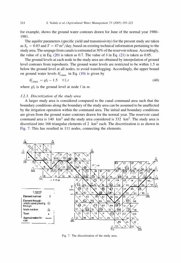
3.2.3. Discretization of the study area
A larger study area is considered compared to the canal command area such that the
boundary conditions along the boundary of the study area can be assumed to be unaffected
by the irrigation operation within the command area. The initial and boundary conditions
are given from the ground water contours drawn for the normal year. The reservoir canal
command area is 140 km2 and the study area considered is 332 km2. The study area is
discretized into 166 triangular elements of 2 km2 each. The discretization is as shown in
Fig. 7. This has resulted in 111 nodes, connecting the elements.
S. Vedula et al. / Agricultural Water Management 73 (2005) 193–221214
Fig. 7. The discretization of the study area.
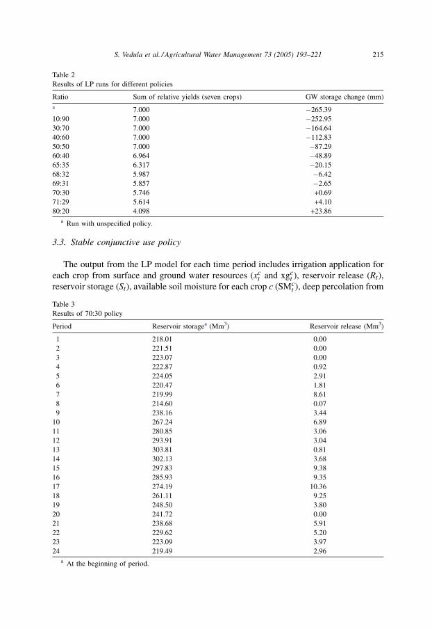
3.3. Stable conjunctive use policy
The output from the LP model for each time period includes irrigation application for
each crop from surface and ground water resources (xct and xgc
t ), reservoir release (Rt),
reservoir storage (St), available soil moisture for each crop c (SMct ), deep percolation from
S. Vedula et al. / Agricultural Water Management 73 (2005) 193–221 215
Table 2
Results of LP runs for different policies
Ratio Sum of relative yields (seven crops) GW storage change (mm)
a 7.000 �265.39
10:90 7.000 �252.95
30:70 7.000 �164.64
40:60 7.000 �112.83
50:50 7.000 �87.29
60:40 6.964 �48.89
65:35 6.317 �20.15
68:32 5.987 �6.42
69:31 5.857 �2.65
70:30 5.746 +0.69
71:29 5.614 +4.10
80:20 4.098 +23.86
a Run with unspecified policy.
Table 3
Results of 70:30 policy
Period Reservoir storagea (Mm3) Reservoir release (Mm3)
1 218.01 0.00
2 221.51 0.00
3 223.07 0.00
4 222.87 0.92
5 224.05 2.91
6 220.47 1.81
7 219.99 8.61
8 214.60 0.07
9 238.16 3.44
10 267.24 6.89
11 280.85 3.06
12 293.91 3.04
13 303.81 0.81
14 302.13 3.68
15 297.83 9.38
16 285.93 9.35
17 274.19 10.36
18 261.11 9.25
19 248.50 3.80
20 241.72 0.00
21 238.68 5.91
22 229.62 5.20
23 223.09 3.97
24 219.49 2.96
a At the beginning of period.

the root zone of each crop (DPct ) and the ground water levels at each node l (ht
l). Without
any restriction on the groundwater pumping the objective function value, which is the sum
of the relative yields of crops, obtained is 7.00. The annual ground water balance
components are computed for the entire study area for this run. The resulting annual ground
water storage change is �265:39 mm, which is too high for a stable condition. Therefore,
the conjunctive use model is run for different pre-determined ratios of annual surface and
ground water applications and the results analyzed. A 60:40 policy refers to a case where
60% of the annual irrigation application at the crop level comes from surface source and
40% through ground water pumping. Ground water balance components over the entire
study area are calculated for each of these runs as mentioned earlier.
The results of these runs are presented in Table 2. It is observed from the table that, as
the proportion of ground water pumping is reduced, there is a progressive improvement in
the ground water storage change position. It is noticed, that as ground water allocation is
reduced, the sum of relative yield decreases indicating that the crops get decreasing amount
of water for their requirement. The maximum of the sum of relative yield is 7.0, as there are
seven crops. If crop water demands are not fully met in all the periods of the crop season,
this value reduces depending on the water deficit experienced. The 70:30 policy, however,
resulted in an annual change in ground water storage of +0.69 mm which is considered
negligible. Thus 70:30 policy is considered as the ‘‘stable policy’’. The sum of relative
yields corresponding to this policy is 5.746 (as against the maximum 7.0). The reservoir
S. Vedula et al. / Agricultural Water Management 73 (2005) 193–221216
Table 4
Results of 70:30 policy for ground nut (K)
Period SM (mm/cm) x (mm) xg (mm) AET (mm) PET (mm) DP (mm)
3 2.50 0.00 0.00 33.71 33.71 0.0
4 2.07 0.00 0.00 33.71 33.71 0.0
5 2.14 0.00 0.00 37.96 56.78 0.0
6 1.99 0.00 0.00 0.00 56.78 0.0
7 2.50 43.73 0.00 77.40 77.40 0.0
8 2.44 0.00 0.00 77.40 77.40 0.0
9 2.50 16.55 0.00 84.60 84.60 0.0
10 2.50 37.95 0.00 84.60 84.60 0.0
11 2.50 7.93 0.00 37.46 37.46 0.0
SM: available soil moisture, x: surface water allocation, xg: ground water allocation, AET: actual evapotranspira-
tion, PET: potential evapotranspiration, DP: deep percolation.
Table 5
Results of 70:30 policy for maize (R)
Period SM (mm/cm) x (mm) xg (mm) AET (mm) PET (mm) DP (mm)
14 2.50 22.68 0.00 26.02 26.02 0.0
15 2.50 65.48 0.00 67.36 67.36 0.0
16 2.50 61.50 4.94 67.36 67.36 0.0
17 2.50 15.25 87.46 105.00 105.00 0.0
18 2.50 0.00 88.99 105.00 105.00 0.0
19 2.38 0.00 0.00 0.00 109.18 0.0
20 2.40 0.00 0.00 0.00 109.18 0.0
21 2.42 0.00 0.00 0.00 65.53 0.0

storages at the beginning of each period and the reservoir releases resulted from this run are
given in Table 3. The surface and ground water allocations in each time period, the actual
evapotranspiration values in each period, the available soil moisture values for each period
resulted from this run for two of the crops, one each in Kharif and Rabi seasons are given in
Tables 4 and 5. The ground water balance components computed from the results of this
run (70:30) are given in Table 6. It is seen from the table that the rainfall recharge roughly
equals the net ground water outflow, while the canal recharge equals the ground water
pumping in the study area resulting in a negligible (+0.68 mm) change in the ground water
level.
S. Vedula et al. / Agricultural Water Management 73 (2005) 193–221 217
Table 6
GW balance components for 70:30 policy (normal year)
mm
Rainfall recharge 15.60
Canal recharge 86.20
GW pumping 86.36
Net GW outflow 14.76
Change in GW storage 0.68
Table 7
Values of rt with 70:30 policy
Period 100 rt
1 0.00
2 0.00
3 0.00
4 100.00
5 100.00
6 100.00
7 100.00
8 100.00
9 100.00
10 96.14
11 81.86
12 67.19
13 100.00
14 67.46
15 70.89
16 70.16
17 50.42
18 48.24
19 46.65
20 0.00
21 100.00
22 100.00
23 100.00
24 100.00

3.3.1. Stable policy parameters
As mentioned earlier, the stable policy is characterized by two parameters, which vary
with the time period. One is rt, which is the ratio of the quantum of surface water allocated
to the total water allocated in period t, for all crops together. The other is act , which is the
ratio of the actual to potential evapotranspiration for crop c in period t. The values of these
parameters, for the identified stable policy (70:30 policy) are given in Tables 7 and 8
(Table 7 containing values of rt, and Table 8 of act ).
S. Vedula et al. / Agricultural Water Management 73 (2005) 193–221218
Table 8
Values of act with 70:30 policy for different crops
Period Paddy (K) Ground nut Cotton Paddy (R) Maize Sunflower Sugarcane
1 0.3669
2 0.0000
3 1.0000 1.0000
4 1.0000 1.0000 1.0000 0.8652
5 1.0000 0.6685 1.0000 0.6737
6 1.0000 0.0000 1.0000 0.5885
7 1.0000 1.0000 1.0000 0.0000
8 1.0000 1.0000 1.0000 0.0000
9 1.0000 1.0000 1.0000 0.4812
10 1.0000 1.0000 1.0000 0.0000
11 1.0000 1.0000 1.0000 1.0000
12 1.0000 1.0000 1.0000
13 1.0000
14 1.0000 1.0000 1.0000 1.0000
15 1.0000 1.0000 1.0000 1.0000
16 1.0000 1.0000 1.0000 1.0000
17 1.0000 1.0000 1.0000 1.0000
18 1.0000 1.0000 1.0000 1.0000
19 1.0000 0.0000 1.0000 1.0000
20 1.0000 0.0000 1.0000 0.8830
21 1.0000 0.0000 1.0000 0.4439
22 1.0000 1.0000 0.3545
23 0.8609
24 1.0000
Table 9
Results of simulationa (all crops, 70:30 policy)
Year GW storage change (mm)
1 +7.83
2 +14.88
3 +20.15
4 +8.16
5 +1.45
6 +7.08
7 +15.78
8 -9.52
a June 1978–May 1986 (eight water years).

The annual change in storage for each year as obtained from the simulation run is
given in Table 9. The net increase in storage over 8 years is 65.81 mm, which works out to
an average of 8.23 mm/year. The corresponding rate of rise of the average ground water
level over the study area is 0.274 m per year which is considered acceptable. It is observed
from the simulation results thus, that the application of the 70:30 stable optimal
conjunctive use policy has resulted in a near stable ground water regime in the command
area.
4. Summary and conclusions
A mathematical model (LP) is developed for optimal conjunctive use planning in
multicrop irrigation in a canal command area to maximize the sum of annual relative yields
of crops in a normal year. The system is characterized by three main components: the
reservoir, the irrigated area and the underlying aquifer with the associated dynamic
relationships defining the interaction among them. The model considers varying soil
moisture conditions and soil types and takes into account the dynamic response of the
aquifer in the irrigated area to surface application, pumping and recharge. The constraint
sets are the mass balance of the reservoir storage, soil moisture continuity in the cropped
area, and the governing equations for ground water flow. These sets of constraints are
linked together appropriately by additional constraints.
A two-dimensional, isotropic, homogeneous unconfined aquifer is modeled through a
finite element ground water model. The governing partial differential equations
representing groundwater flow are transformed into linear algebraic equations using
Galarkin method of weighted residuals. These equations are written for each node and
embedded into the optimization model as constraints.
Concept of a conjunctive use policy and a stable conjunctive policy are defined and the
methodology of determining such a policy for a given canal command area is illustrated
with model application to an existing reservoir command area in the state of Karnataka,
India. The particular policy, for which the annual change in ground water storage is
negligible when the model is run for a normal year, is identified as a ‘‘stable policy’’.
The real time implementation of the stable policy arrived through optimization is
illustrated through a simulation model and applied to the case of an existing reservoir in
Karnataka State, India.
References
Aron, G., 1969. Optimization of conjunctively managed surface and ground water resources by dynamic
programming, Contribution no. 129. Water Resource Center, University of California.
Azaiez, M.N., Hariga, M., 2001. A single-period model for conjunctive use of ground and surface water under
severe overdrafts and water deficit. Eur. J. Oper. Res. 133 (3), 653–666.
Barlow, P.M., Ahlfeld, D.P., Dickerman, D.C., 2003. Conjunctive-management models for sustained yield of
stream–aquifer systems. J. Water Res. Plann. Manage. 129 (1), 35–48.
Belaineh, G., Peralta, R.C., Hughes, T.C., 1999. Simulation/optimization modeling for water resources manage-
ment. J. Water Res. Plann. Manage. 125 (3), 154–161.
S. Vedula et al. / Agricultural Water Management 73 (2005) 193–221 219

Bredehoeft, J.D., Young, R.A., 1970. The temporal allocation of ground water – a simulation approach. Water
Resour. Res. 6 (1), 3–21.
Bredehoeft, J.D., Young, R.A., 1983. Conjunctive use of groundwater and surface water for irrigated agriculture:
risk aversion. Water Resour. Res. 19 (5), 1111–1121.
Buras, N., 1963. Conjunctive operation of dams and aquifers. J. Hydraul. Div., ASCE 89 (6), 111–131.
Chandra Sekhar, G., 1998. Conjunctive use modelling for multicrop irrigation. Ph.D. Thesis. Department of Civil
Engineering, Indian Institute of Science, Bangalore, India.
Chaves-Morales, J., Marino, M.A., Holzapfel, A.H., 1992. Planning simulation model of irrigation district. J. Irrig.
Drainage Eng., ASCE 118 (1), 74–87.
Chun, R.Y.D., Mitchell, L.R., Mido, K.W., 1964. Ground water management for the nation’s future – optimum
conjunctive operation of ground water basin. J. Hydraul. Div., ASCE 90 (4), 79–95.
Cochran, G.F., Butcher, W.S., 1970. Dynamic programming for optimum conjunctive use. Water Res. Bull. 6 (3),
311–322.
Coskunoglu, O., Shetty, C.M., 1981. Optimal stream–aquifer development. J. Water Resour. Plann. Manage. Div.,
ASCE 107 (2), 513–531.
Doorenbos, J., Kassam, A.H., 1979. Yield response to water, FAO irrigation and drainage paper no. 33. Food and
Agriculture Organisation of the United Nations, Rome, Italy.
Dreizin, Y.C., Haimes, Y.Y., 1977. A hierarchy of response functions for ground water management. Water Resour.
Res. 13 (1), 78–86.
Haimes, Y.Y., Dreizin, Y.C., 1977. Management of groundwater and surface water via decomposition. Water
Resour. Res. 13 (1), 69–77.
Jones, L.D., Willis, R., Yeh, W.W-G., 1987. Optimal control of nonlinear ground water hydraulics using
differential dynamic programming. Water Resour. Res. 23 (11), 2097–2106.
Lakshminarayana, V., Rajagopalan, P., 1977. Optimal cropping pattern for basin in India. J. Irrig. Drainage Eng.
Div., ASCE 103 (1), 53–70.
Latif, M., James, L.D., 1991. Conjunctive water use to control waterlogging and salinization. J. Water Resour.
Plann. Manage. Div., ASCE 117 (6), 611–628.
Maddock III, T., 1972. Algebraic technological function from a simulation model. Water Resour. Res. 8 (1), 129–
134.
Maddock III, T., 1973. Management model as a tool for studying the worth of data. Water Resour. Res. 9 (2), 270–
280.
Marino, M.A., 2001. Conjunctive Management of Surface Water and Groundwater, Issue 268. IAHS-AISH
Publication, pp. 165–173.
Matsukawa, J., Finney, B.A., Willis, R., 1992. Conjunctive use planning in Mad river basin, California. J. Water
Resour. Plann. Manage., ASCE 118 (2), 115–132.
Morel-Seytoux, H.J., 1975. A simple case of conjunctive surface ground water management. Ground Water 10 (6),
506–515.
Nieswand, G.H., Granstrom, M.L., 1971. A chance constrained approach to the conjunctive use of surface waters
and groundwaters. Water Resour. Res. 7 (6), 1425–1436.
O’Mara, G.T., Duloy, J.H., 1984. Modeling efficient water allocation in a conjunctive use regime. The Indus basin
of Pakistan. Water Resour. Res. 20 (11), 1489–1498.
Onta, P.R., Gupta, A.D., Harboe, R., 1991. Multistep planning model for conjunctive use of surface and ground-
water resources. J. Water Resour. Plann. Manage. 117 (6), 662–678.
Paudyal, G.N., Gupta, A.D., 1990. Irrigation planning by multilevel optimization. J. Irrig. Drainage Eng., ASCE
116 (2), 273–291.
Provencher, B., Burt, O., 1994. Approximating the optimal ground water pumping policy in a multiaquifer
stochastic conjunctive use setting. Water Resour. Res. 30 (3), 833–843.
Rao, S.V.N., Bhallamudi, S.M., Thandaveswara, B.S., Mishra, G.C., 2004. Conjunctive use of surface and
groundwater for coastal and deltaic systems. J. Water Resour. Plann. Manage. 130 (3), 255–267.
Rogers, P., Smith, D.V., 1970. The integrated use of ground and surface water in irrigation project planning. Am. J.
Agric. Econ. 52 (1), 13–24.
Vedula, S., Mujumdar, P.P., 1992. Optimal reservoir operation for irrigation of multiple crops. Water Resour. Res.
28 (1), 1–9.
S. Vedula et al. / Agricultural Water Management 73 (2005) 193–221220

Vedula, S., Nagesh Kumar, D., 1996. An integrated model for optimal reservoir operation for irrigation of multiple
crops. Water Resour. Res. 32 (4), 1101–1108.
Willis, R., Finney, B.A., Zhang, D., 1989. Water resources management in north China plain. J. Water Res. Plann.
Manage. Div., ASCE 115 (5), 598–615.
Yeh, W.W.-G., 1992. System analysis in ground water planning and management. J. Water Resour. Plann.
Manage., ASCE 118 (3), 224–237.
Yu, W., Haimes, Y.Y., 1974. Multilevel optimization for conjunctive use of groundwater and surface water. Water
Resour. Res. 10 (4), 625–636.
S. Vedula et al. / Agricultural Water Management 73 (2005) 193–221 221


![[Slide] Containment Conjunctive Queries](https://static.cupdf.com/doc/110x72/5695d2de1a28ab9b029c044a/slide-containment-conjunctive-queries.jpg)