Dynamic Article LinksC<Energy &Environmental Science
Cite this: Energy Environ. Sci., 2012, 5, 9055
www.rsc.org/ees PAPER
Dow
nloa
ded
by C
alif
orni
a In
stitu
te o
f T
echn
olog
y on
25
Oct
ober
201
2Pu
blis
hed
on 3
1 A
ugus
t 201
2 on
http
://pu
bs.r
sc.o
rg |
doi:1
0.10
39/C
2EE
2224
8EView Online / Journal Homepage / Table of Contents for this issue
Concentrated solar thermoelectric generators†
Lauryn L. Baranowski,a G. Jeffrey Snyderb and Eric S. Toberer*c
Received 17th May 2012, Accepted 6th August 2012
DOI: 10.1039/c2ee22248e
Solar thermoelectric generators (STEGs) are solid state heat engines that generate electricity from
concentrated sunlight. In this paper, we develop a novel detailed balance model for STEGs and apply
this model to both state-of-the-art and idealized materials. This model uses thermoelectric
compatibility theory to provide analytic solutions to device efficiency in idealized materials with
temperature-dependent properties. The results of this modeling allow us to predict maximum
theoretical STEG efficiencies and suggest general design rules for STEGs. With today’s materials, a
STEG with an incident flux of 100 kWm�2 and a hot side temperature of 1000 �C could achieve 15.9%
generator efficiency, making STEGs competitive with concentrated solar power plants. Future
developments will depend on materials that can provide higher operating temperatures or higher
material efficiency. For example, a STEG with zT ¼ 2 at 1500 �C would have an efficiency of 30.6%.
Introduction
There are many technologies available to directly harness the
sun’s energy, the most prevalent of which are photovoltaics and
solar thermal (also known as concentrated solar power). Solar
thermal technologies produce electric power from a temperature
gradient, traditionally by using conventional heat engines.1 Solid
state heat engines, in the form of thermoelectric generators
(TEGs), can also exploit this temperature gradient to generate
power.2
A thermoelectric (TE) material generates a voltage in response
to a temperature gradient. The efficiency of a thermoelectric
aMaterials Science, Colorado School of Mines, Golden, CO 80401, USAbMaterials Science, California Institute of Technology, Pasadena, CA91125, USAcDepartment of Physics, Colorado School of Mines, Golden, CO 80401,USA. E-mail: [email protected]
† Electronic supplementary information (ESI) available. See DOI:10.1039/c2ee22248e
Broader context
Technologies that can directly harness the sun’s energy are becomin
prevalent of which are photovoltaics and solar thermal (also know
which use conventional heat engines to generate electric power from
Solar thermoelectric generators (STEGs), which are solid state heat
operate at higher temperatures than CSP systems and do not requ
develop a detailed balance approach to deriving the maximum th
selective absorber to efficiently capture the incident solar flux, whi
today’s materials (zT¼ 1) and a hot side temperature of 1000 �C cou
With reasonable improvements in thermoelectric materials (zT ¼ 2
temperature and level of illumination.
This journal is ª The Royal Society of Chemistry 2012
material is governed by its figure of merit, zT, defined as
zT ¼ a2T
kr, where a is the Seebeck coefficient, k the thermal
conductivity, and r the electrical resistivity. Until recently,
thermoelectric materials had demonstrated peak zT values of
0.5–0.8, leading to low conversion efficiencies and limiting these
materials to niche applications.3
With the advent of nanostructured thermoelectrics and
complex bulk materials in the 1990s, there has been a sharp
increase in zT.2,4–7 Fig. 1 shows advanced materials that exhibit
zT values well in excess of unity over a broad range of temper-
atures. These high performing materials have led to a record of
15% unicouple efficiency reported by the Jet Propulsion Labo-
ratory in 2012.8
In light of these recent developments, we consider solar ther-
moelectric generators (STEGs). In this work, we concentrate our
analysis on high efficiency, concentrated STEGs. STEGs have
several advantages as compared to existing solar technologies.
Unlike traditional solar thermal generators, STEGs are solid
g increasingly important in today’s energy landscape, the most
n as concentrated solar power, or CSP). Installed CSP plants,
a temperature gradient, typically operate at 14–16% efficiency.
engines, represent an alternative to traditional CSP. STEGs can
ire moving generator parts or working fluids. In this paper, we
eoretical STEG efficiency. Our optimized STEG uses a solar
le limiting radiative losses. We predict that a STEG made with
ld achieve an efficiency of 15.9% under illumination by 100 suns.
), we expect a limiting efficiency of 23.5% for the same hot side
Energy Environ. Sci., 2012, 5, 9055–9067 | 9055

Fig. 2 (a): A STEG can be broken down into five subsystems. (1) Optical
concentration. (2) Thermal absorber. (3) Thermoelectric module. (4)
Cooling system. (5) Vacuum encapsulation. (b) Energy incident upon the
selective absorber (qinc) is either absorbed (qabs) or reflected (qref). Some
of the absorbed energy is re-radiated to the atmosphere (qrad), and the
rest is transferred to the TE (qTE). Radiation insulation to prevent heat
loss on the back side of the absorber is not shown.
Fig. 1 Advanced thermoelectric materials demonstrate zT values well
above 1, for both n- and p-type materials. This represents a distinct
improvement over traditional materials, which possess peak zT values
between 0.5 and 0.8. Data from ref. 9–16.
Dow
nloa
ded
by C
alif
orni
a In
stitu
te o
f T
echn
olog
y on
25
Oct
ober
201
2Pu
blis
hed
on 3
1 A
ugus
t 201
2 on
http
://pu
bs.r
sc.o
rg |
doi:1
0.10
39/C
2EE
2224
8E
View Online
state devices with no moving parts, which greatly increases reli-
ability and lifetime. Additionally, STEGs are a scalable tech-
nology that can be used for small- or large-scale applications.
While photovoltaics are limited to the fraction of incident solar
radiation above the bandgap, STEGs utilize a larger portion of
the solar spectrum.
Basic STEG design
The TE efficiency within the STEG is defined as the ratio of the
output electric work to the input heat. Like all heat engines, the
efficiency of TEGs is limited by the Carnot efficiency. For a fixed
cold side temperature (Tc), an increase in the hot side tempera-
ture (Th) will result in a higher total efficiency of the thermo-
electric generator. In order to achieve high values of Th, we look
to high levels of optical concentration, as well as optical and
thermal concentration systems with high efficiencies.
The total efficiency of a STEG depends on the optical,
absorber, and thermoelectric subsystem efficiencies. A STEG can
be divided into several subsystems, as seen in Fig. 2a. The first is
an optical system to concentrate the solar radiation. Second, a
thermal absorber converts the incident light to heat, which then
flows to the thermoelectric module. The cold side temperature of
the TE is maintained by a passive or active cooling system.
Finally, the thermal absorber, TE module, and cooling system
are encapsulated in a vacuum enclosure to prevent conductive
and convective heat losses to the air. The vacuum enclosure could
be similar to those used in evacuated solar hot water systems,
which are widely used and have demonstrated lifetimes greater
than 15 years.17
Optical concentration systems for high efficiency STEGs
would be the same as those used for concentrated photovoltaic or
solar thermal applications.1 These include Fresnel lenses, helio-
stats in conjunction with a central receiver system, and parabolic
dishes and troughs. For use in a STEG, the pertinent charac-
teristics are the level of concentration reached, the tracking
system required, and the optical efficiency.
The optical concentration ratio is defined as the ratio of the
optical concentrator area (i.e., the area of the lens or mirror that
receives the incident light) to the absorber area upon which the
9056 | Energy Environ. Sci., 2012, 5, 9055–9067
light is focused. Considering one sun to be approximately
1 kW m�2, the flux after concentration is given by this solar flux
multiplied by the optical concentration ratio. The concentration
ratio is mainly limited by the type of solar tracking used. For a
static concentrator, with no tracking, the optical concentration
ratio is limited to about 10. When single-axis tracking is intro-
duced, a concentration ratio of 100 can be achieved, above which
dual-axis tracking systems are required.18
The optical efficiency is the ratio of light that reaches the
absorber to the total light incident upon the optical concentrator,
and increases with improved tracking systems. Typical optical
efficiencies are 40% for static concentrators, 60% for single-axis
tracking, and 85–90% for dual-axis tracking.19 With dual-axis
tracking, the optical losses of the tracking system itself are very
low; other losses due to factors such as soiling of the lens surface,
reflection, and absorption are still present.20 It is also important
to remember that increased tracking increases the system cost.
In order for the thermal absorber to effectively convert the
incident light to heat, the surface must have a high absorptivity.
However, by Kirchhoff’s Law, this also invokes a high emis-
sivity, leading to large radiative losses. This conflict can be
This journal is ª The Royal Society of Chemistry 2012
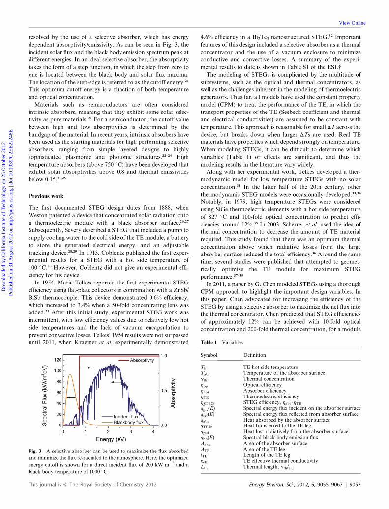
Table 1 Variables
Dow
nloa
ded
by C
alif
orni
a In
stitu
te o
f T
echn
olog
y on
25
Oct
ober
201
2Pu
blis
hed
on 3
1 A
ugus
t 201
2 on
http
://pu
bs.r
sc.o
rg |
doi:1
0.10
39/C
2EE
2224
8E
View Online
resolved by the use of a selective absorber, which has energy
dependent absorptivity/emissivity. As can be seen in Fig. 3, the
incident solar flux and the black body emission spectrum peak at
different energies. In an ideal selective absorber, the absorptivity
takes the form of a step function, in which the step from zero to
one is located between the black body and solar flux maxima.
The location of the step-edge is referred to as the cutoff energy.21
This optimum cutoff energy is a function of both temperature
and optical concentration.
Materials such as semiconductors are often considered
intrinsic absorbers, meaning that they exhibit some solar selec-
tivity as pure materials.22 For a semiconductor, the cutoff value
between high and low absorptivities is determined by the
bandgap of the material. In recent years, intrinsic absorbers have
been used as the starting materials for high performing selective
absorbers, ranging from simple layered designs to highly
sophisticated plasmonic and photonic structures.22–24 High
temperature absorbers (above 750 �C) have been developed that
exhibit solar absorptivities above 0.8 and thermal emissivities
below 0.15.21,25
Previous work
The first documented STEG design dates from 1888, when
Weston patented a device that concentrated solar radiation onto
a thermoelectric module with a black absorber surface.26,27
Subsequently, Severy described a STEG that included a pump to
supply cooling water to the cold side of the TE module, a battery
to store the generated electrical energy, and an adjustable
tracking device.28,29 In 1913, Coblentz published the first exper-
imental results for a STEG with a hot side temperature of
100 �C.30 However, Coblentz did not give an experimental effi-
ciency for his device.
In 1954, Maria Telkes reported the first experimental STEG
efficiency using flat-plate collectors in combination with a ZnSb/
BiSb thermocouple. This device demonstrated 0.6% efficiency,
which increased to 3.4% when a 50-fold concentrating lens was
added.31 After this initial study, experimental STEG work was
intermittent, with low efficiency values due to relatively low hot
side temperatures and the lack of vacuum encapsulation to
prevent convective losses. Telkes’ 1954 results were not surpassed
until 2011, when Kraemer et al. experimentally demonstrated
Fig. 3 A selective absorber can be used to maximize the flux absorbed
and minimize the flux re-radiated to the atmosphere. Here, the optimized
energy cutoff is shown for a direct incident flux of 200 kW m�2 and a
black body temperature of 1000 �C.
This journal is ª The Royal Society of Chemistry 2012
4.6% efficiency in a Bi2Te3 nanostructured STEG.32 Important
features of this design included a selective absorber as a thermal
concentrator and the use of a vacuum enclosure to minimize
conductive and convective losses. A summary of the experi-
mental results to date is shown in Table S1 of the ESI.†
The modeling of STEGs is complicated by the multitude of
subsystems, such as the optical and thermal concentrators, as
well as the challenges inherent in the modeling of thermoelectric
generators. Thus far, all models have used the constant property
model (CPM) to treat the performance of the TE, in which the
transport properties of the TE (Seebeck coefficient and thermal
and electrical conductivities) are assumed to be constant with
temperature. This approach is reasonable for small DT across the
device, but breaks down when larger DTs are used. Real TE
materials have properties which depend strongly on temperature.
When modeling STEGs, it can be difficult to determine which
variables (Table 1) or effects are significant, and thus the
modeling results in the literature vary widely.
Along with her experimental work, Telkes developed a ther-
modynamic model for low temperature STEGs with no solar
concentration.31 In the latter half of the 20th century, other
thermodynamic STEG models were occasionally developed.33,34
Notably, in 1979, high temperature STEGs were considered
using SiGe thermoelectric elements with a hot side temperature
of 827 �C and 100-fold optical concentration to predict effi-
ciencies around 12%.35 In 2003, Scherrer et al. used the idea of
thermal concentration to decrease the amount of TE material
required. This study found that there was an optimum thermal
concentration above which radiative losses from the large
absorber surface reduced the total efficiency.36 Around the same
time, several studies were published that attempted to geomet-
rically optimize the TE module for maximum STEG
performance.37–39
In 2011, a paper by G. Chen modeled STEGs using a thorough
CPM approach to highlight the important design variables. In
this paper, Chen advocated for increasing the efficiency of the
STEG by using a selective absorber to maximize the net flux into
the thermal concentrator. Chen predicted that STEG efficiencies
of approximately 12% can be achieved with 10-fold optical
concentration and 200-fold thermal concentration, for a module
Symbol Definition
Th TE hot side temperatureTabs Temperature of the absorber surfacegth Thermal concentrationhop Optical efficiencyhabs Absorber efficiencyhTE Thermoelectric efficiencyhSTEG STEG efficiency, habs$hTEq0 0inc(E) Spectral energy flux incident on the absorber surfaceq0 0ref(E) Spectral energy flux reflected from absorber surfaceqabs Heat absorbed by the absorber surfaceqTE,in Heat transferred to the TE legqrad Heat lost radiatively from the absorber surfaceq0 0bb(E) Spectral black body emission fluxAabs Area of the absorber surfaceATE Area of the TE leglTE Length of the TE legkeff TE effective thermal conductivityLth Thermal length, gthlTE
Energy Environ. Sci., 2012, 5, 9055–9067 | 9057

Dow
nloa
ded
by C
alif
orni
a In
stitu
te o
f T
echn
olog
y on
25
Oct
ober
201
2Pu
blis
hed
on 3
1 A
ugus
t 201
2 on
http
://pu
bs.r
sc.o
rg |
doi:1
0.10
39/C
2EE
2224
8E
View Online
operating at 527 �C with an average zT of 1.17 Following shortly
thereafter, a paper by McEnaney et al. modeled segmented and
cascaded Bi2Te3/skutterudite STEGs, using data from currently
existing thermoelectric materials and selective surfaces. The
efficiency of the cascaded design was predicted to be the highest,
reaching 16% at 600 �C.40 While this study did much to shed light
on the important design variables of a STEG, the predicted
device performance was determined by finite element modeling
for a specific generator design and TE materials. Thus to date,
STEG modeling efforts have been numerical approaches or have
used CPM to address TE performance, limiting the applicability
of these models.
In this study, we develop a generalized description of STEGs
that is analytic and is not limited by CPM. We consider opti-
mized TE geometries, selective absorbers, and total efficiencies
for given optical and thermal concentrations. This global opti-
mization is done from the view of a fixed hot side temperature,
because of the inherent temperature limits of TE materials. We
finish by using advanced TE materials’ experimental data to
design an optimized STEG module.
Methods
In deriving the total system efficiency, we separate the optical
efficiency from the STEG efficiency. The STEG can be broken
down into two subsystems: the thermal absorber and the TEG.
The efficiency for each subsystem can be derived individually,
and the STEG efficiency is simply the product of the two. The
absorber efficiency is defined as the ratio of the heat transferred
to the TE to the total heat that strikes the absorber surface. We
must first consider the modeling of the selective absorber to
determine how much of this incident heat is actually absorbed by
the surface. Then, the absorber efficiency is derived using heat
transfer modeling to consider the conductive and radiative heat
flows within the absorber and the TE leg. The thermoelectric
efficiency is derived for model materials with a temperature
independent zT and for real materials in a cascaded generator.
Heat transfer modeling
In the following thermodynamic analysis, we can define spectral
heat fluxes, which represent power per unit area per unit energy,
total heat fluxes, which represent power per unit area, and heat
rates, which represent energy per unit time (power). In the
following sections, spectral heat fluxes are represented by q00(E),and have units of kW m�2 eV�1 and total heat fluxes will be
represented by q00 and are in units of kW m�2. Heat rates will be
represented by q00 in units of kW. Integration of the spectral heat
flux gives the total heat flux: q00 ¼ðq00ðEÞdE. The total heat flux
Table 2 Fixed parameters
Symbol Definition Value
Tc TE cold side temperature 100 �Cq0 0sun(E) Spectral solar energy flux AM 1.5 direct spectrum (scaled)as(E) Spectral absorptivity 1, E > cutoff energy, 0 otherwisezT TE figure of merit 1, 2kTE TE thermal conductivity 1 W m�1 K�1
9058 | Energy Environ. Sci., 2012, 5, 9055–9067
and the heat rate can be related to each other through the area of
the surface in question, so that q ¼ q0 0A. The pertinent heat ratesfor the system are shown in Fig. 2b.
After passing through the optical concentration system, the
concentrated solar flux is transmitted through the vacuum
enclosure and is incident upon the surface of the absorber (q0 0inc).
Here, the spectral solar flux (q0 0sun(E)) is given by the AM 1.5
direct spectrum (version G173-03), which yields 0.9 kW m�2
when integrated over the entire spectrum (Table 2). This solar
flux is concentrated by the optical system to give a final value of
q0 0inc(E).
An ideal selective absorber is a material in which the absorp-
tivity exhibits a step edge between zero and one at a specific value
of energy referred to as the cutoff energy (an example of this
function can be seen in Fig. 3). We define the optimal cutoff
energy as that which results in the highest net flux into the
absorber (q0 0abs � q
0 0rad). As the energy cutoff is a function of both
the absorber temperature and the incident flux, we iteratively
determine an optimum energy cutoff for each combination of
these variables.
The absorber surface is not a perfect black body, and thus only a
fraction of the incident energy is absorbed (q0 0abs) and the remainder
is reflected back into the atmosphere (q0 0ref). The energyabsorbedby
the surface can be related to the total incident energy as:
qabs ¼ Aabs
ðN0
asðEÞq00incðEÞdE (1)
where as(E) is the spectral absorptivity, andAabs is the area of the
absorber surface. Here, integration over all energies gives the
total value of qabs. This expression, as well as the following
expression for the radiative heat loss (eqn (4)), is based on the
same detailed balance principle that is used to calculate the
maximum efficiency of photovoltaic devices.41
To consider the heat flow within the absorber, we assume the
STEG is sufficiently well-designed that some losses may be
neglected in our heat balance. First, we expect that the heat lost
through convection will be minimal by enclosing the absorber
and thermoelectric legs in a vacuum enclosure, as shown in
Fig. 2a. Second, we assume design elements such as insulation
and heat shielding are implemented to minimize the heat loss
from the sides and back of the absorber. Finally, we assume a
perfect selective absorber and neglect reflection losses in the
absorbing region.
In this limit, the heat absorbed by the surface can either be re-
radiated to the atmosphere (qrad) or flow to the TE (qTE,in), as
shown in Fig. 2b. This can be represented by the following heat
balance:
qabs ¼ qTE,in + qrad (2)
We can then define the absorber efficiency as:
habshqTE;in
qinc¼ qabs � qrad
qinc¼ q
00abs � q
00rad
q00inc
(3)
Any heat which does not flow through the thermoelectric
module is considered a parasitic loss.
Following Kirchhoff’s law of thermal radiation (a(E) ¼ 3(E)),
the radiative heat loss is calculated by integrating the product of
the spectral emissivity and the black body emission spectrum:
This journal is ª The Royal Society of Chemistry 2012

Dow
nloa
ded
by C
alif
orni
a In
stitu
te o
f T
echn
olog
y on
25
Oct
ober
201
2Pu
blis
hed
on 3
1 A
ugus
t 201
2 on
http
://pu
bs.r
sc.o
rg |
doi:1
0.10
39/C
2EE
2224
8E
View Online
qrad ¼ Aabsp
ðN0
3sðEÞq00bbðEÞdE
q00bbðEÞ ¼
2E3
c2h31
eE=kBT � 1
(4)
in which the factor of p is the result of integration over a half-
sphere.
Quantifying the radiative loss from the absorber via eqn (4)
requires determining the temperature of the absorber surface
(Tabs), which will differ from Th. Because of the differences in
magnitude of the thermal conductivity of the absorber (for
example, �55 W m�1 K�1 for graphite at 1000 �C 42) and the TE
(�1 W m�1 K�1), the temperature drop across the absorber will
be very small compared to the drop across the TE. The difference
between Tabs and Th has been calculated, and is less than 0.5% for
most of the variable space, with a maximum difference of 1.5%
(see ESI†). We thus assume that Tabs ¼ Th, which greatly
simplifies the STEG model. We have also assumed that there is
no lateral temperature gradient across the absorber surface. If
the absorber surface is sufficiently thermally conductive, then the
lateral temperature change across the absorber is indeed
minimal. This can be shown by calculating the temperature
distribution over a basic annular fin model, which has been done
by Kraemer et al.32 We have also performed this calculation for
our system, and these data are presented in the ESI.†
We can express the conductive heat transfer into a TE leg of
area ATE and length lTE as:
qTE;in ¼ ðTh � TcÞ keffATE
lTE(5)
In a thermoelectric material, the heat balance is complicated
by the Joule and Thomson effects. While there is significant heat
divergence within a thermoelectric leg (qTE,in s qTE,out), here we
are only concerned with the heat flux entering the leg from the
absorber. In the Appendix, we develop an expression for heat
transfer into the thermoelectric leg in terms of an effective
thermal conductivity (keff, eqn (A.20)). This model rigorously
considers the Joule and Thomson effects in the leg and allows
these terms to be included within a simple Fourier law descrip-
tion of conduction (eqn (5)). To our knowledge, this concept of
effective thermal conductivity in thermoelectrics has not been
considered before.
The absorber efficiency (eqn (3)) describes the ratio of the heat
transferred to the TE leg (qTE) to the total heat incident upon the
absorber (qinc). Thus, the value of the absorber efficiency can be
used to quantify the reflective and radiative losses of the system.
Using our definition of the incident flux, in combination with
eqn (5), yields:
habs ¼ðTh � TcÞkeffATE
q00incAabslTE
(6)
Rather than considering the areas of both the absorber and the
TE, it is simpler to consider the ratio of the two, defined as the
thermal concentration (gth):
gthhAabs
ATE
(7)
We thus obtain an expression for habs which depends on two
geometric parameters: lTE and gth. To simplify our optimization,
This journal is ª The Royal Society of Chemistry 2012
we define a ‘‘thermal length’’: Lth h gth$lTE. Conveniently, an
expression forLth can be developed by combining eqn (3) and (6):
Lth ¼ ðTh � TcÞkeffq00abs � q
00rad
(8)
The numerical value ofLth results from the maximization of the
net flux (q0 0abs � q
0 0rad) for a given q
0 0inc and Th. This is done via the
energy cutoff, and yields an optimized absorber efficiency. The
remaining parameters in eqn (8) (Tc and keff) are chosen to be
100 �C and determined using eqn (A.20), respectively (Table 2).
Thus, theLth value is anoptimized length andnot a freeparameter.
Thermoelectric efficiency
The efficiency of thermoelectric generators has traditionally been
analyzed using the constant property model (CPM), a global
approach to the transport properties.43,44 Recently, a local
approach to generator efficiency has been developed which
greatly simplifies the analysis and optimization. This approach is
derived in ref. 45 and 46; here we review the key features.
This local approach differs from the CPM in that it does not
inherently assume any material properties. Because of the lack of
assumptions in this model, it is necessary to constrain some
parameters in order to reach an analytical solution. Here, we
assume constant thermal conductivity and zT. For many TE
materials, the kTE value varies by less than 50% over a several
hundred degrees temperature range (see, for example, the kTEdata in ref. 9–16). In contrast, the Seebeck coefficient and elec-
trical conductivity often vary by several orders of magnitude over
the same temperature range. Cascaded and segmented generator
designs allow for an approximately constant value of zT.
The macroscopic thermoelectric leg is infinitely divided into
layers which are electrically and thermally in series. The
maximum local efficiency is set by the local Carnot efficiency dT/
T. In practice, the local efficiency is a fraction of dT/T; this
fraction is termed the reduced efficiency hr(T). Thus an ideal
Carnot generator would have an hr(T) of unity for all T. Given
hr(T) across a leg, the global efficiency can be derived:
hTE ¼ 1� exp
��ðTh
Tc
hr
TdT
�(9)
Wewillpursue twoapproaches, thefirstwithgeneralizedmaterial
properties and the second specific to the current state-of-the-art
materials. In both cases, prediction of optimum performance
requires an optimized reduced current density u. In a thermoelectric
leg, the reduced current density can be defined as the ratio of the
electric current density, J, to the heat flux by conduction, kVT.
uhJ
kVT(10)
For a constant kVT, we can see that u is simply a scaled version
of the current density J.
The local reduced efficiency is found to be:
hrðTÞ ¼ uða� rkuÞuaþ 1
T
(11)
By tuning the reduced current density u, hr can be maximized.
The peak in hr occurs when u is equal to the ‘thermoelectric
compatibility factor’ s, which is defined as:
Energy Environ. Sci., 2012, 5, 9055–9067 | 9059
Dow
nloa
ded
by C
alif
orni
a In
stitu
te o
f T
echn
olog
y on
25
Oct
ober
201
2Pu
blis
hed
on 3
1 A
ugus
t 201
2 on
http
://pu
bs.r
sc.o
rg |
doi:1
0.10
39/C
2EE
2224
8E
View Online
sh
ffiffiffiffiffiffiffiffiffiffiffiffiffiffi1þ zT
p � 1
aT(12)
The maximum reduced efficiency, obtained when u ¼ s, is
given by
hr;max ¼ffiffiffiffiffiffiffiffiffiffiffiffiffiffi1þ zT
p � 1ffiffiffiffiffiffiffiffiffiffiffiffiffiffi1þ zT
p þ 1(13)
As a general rule, hr(T) is significantly compromised when u
deviates from s by more than a factor of two.
In our first approach, we assume that u ¼ s across the device.
Cascading allows u to be reset throughout the legs, enabling a
real device to come close (within a factor of two) to u¼ s at all T.
As can be seen in eqn (13), the temperature dependence of zT will
be important in evaluating eqn (9). In a cascaded generator, the
real temperature dependence of zT will have a sawtooth
appearance. Here we approximate zT as a constant. If zT is
constant, then the reduced efficiency is also constant, and the
integral in eqn (9) becomes trivial. With these assumptions, the
global efficiency can be solved to yield:
hTE ¼ 1��Tc
Th
�hr;max
(14)
The second approach considers a cascaded STEG constructed
from state-of-the-art thermoelectric materials with experimen-
tally determined a(T), r(T) and k(T) (and thus zT(T)). The
interface temperatures between stages are set to maximize zT
values. In practice, this typically is the maximum temperature the
lower temperature stage can sustain. This approach maximizes h
for a segment with a given s(T) by iteratively determining the
optimum u(T). The efficiency h is related to the change in ther-
moelectric potential (F) across the device:
h ¼ Fh � Fc
Fh
(15)
The thermoelectric potential is defined as:46
F(T) ¼ (aT + 1/u) (16)
The heat balance equation can be expressed in reduced form:
du
dT¼ u2T
da
dTþ u3rk (17)
This governing expression determines the form of u(T). The
boundary condition for u(T) is iteratively determined to maxi-
mize the global h.
Overall STEG efficiency
The efficiency of the STEG is given by the product of the
absorber and thermoelectric efficiencies (hSTEG¼ habs $ hTE). It is
important to note that we are not including the efficiency of the
optical concentrating system within our value of the
STEG efficiency. This is done to enable more direct comparisons
to other solar energy devices, such as photovoltaics, for which
the reported efficiencies do not include optical concentration
losses.
In the approximation of constant zT and u ¼ s, this yields a
simple expression for STEG efficiency:
9060 | Energy Environ. Sci., 2012, 5, 9055–9067
hSTEG ¼ q00abs � q
00rad
q00inc
�1�
�Tc
Th
�hr�
(18)
The absorber efficiency can also be rewritten in terms of the
physical system design parameters (as in eqn (6)). This gives us an
alternate expression for the STEG efficiency.
hSTEG ¼ ðTh � TcÞkeffq00inc Lth
�1�
�Tc
Th
�hr�
(19)
In the case of a black body (for which the absorptivity is unity
across all energies), the integrals in eqn (1) and (4) become trivial,
and eqn (18) can be written as:
hSTEG ¼ q00inc � sT4
h
q00inc
�1�
�Tc
Th
�hr�
(20)
where s is the Stefan–Boltzmann constant. We emphasize that
the choice of constant zT is to provide analytic solutions within
this paper; a numerical approach can be readily implemented to
solve eqn (13) and (14) and is demonstrated below.
Results and discussion
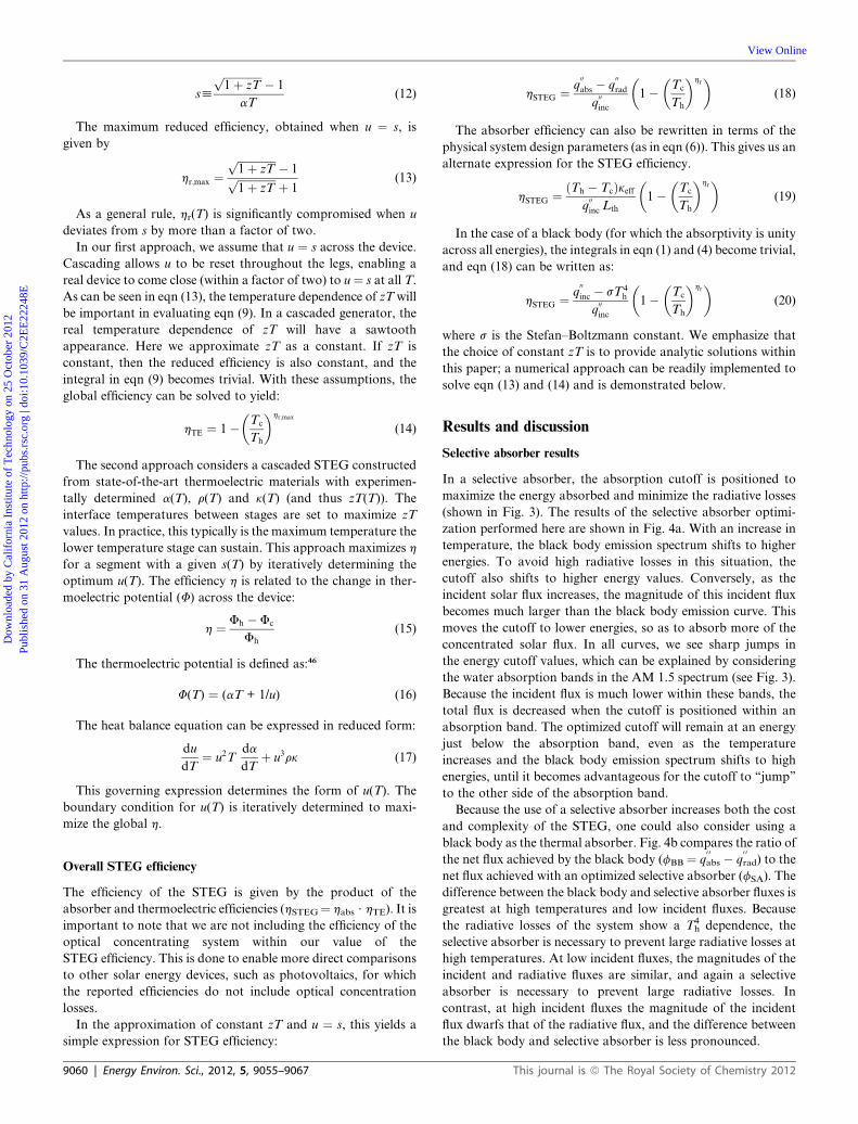
Selective absorber results
In a selective absorber, the absorption cutoff is positioned to
maximize the energy absorbed and minimize the radiative losses
(shown in Fig. 3). The results of the selective absorber optimi-
zation performed here are shown in Fig. 4a. With an increase in
temperature, the black body emission spectrum shifts to higher
energies. To avoid high radiative losses in this situation, the
cutoff also shifts to higher energy values. Conversely, as the
incident solar flux increases, the magnitude of this incident flux
becomes much larger than the black body emission curve. This
moves the cutoff to lower energies, so as to absorb more of the
concentrated solar flux. In all curves, we see sharp jumps in
the energy cutoff values, which can be explained by considering
the water absorption bands in the AM 1.5 spectrum (see Fig. 3).
Because the incident flux is much lower within these bands, the
total flux is decreased when the cutoff is positioned within an
absorption band. The optimized cutoff will remain at an energy
just below the absorption band, even as the temperature
increases and the black body emission spectrum shifts to high
energies, until it becomes advantageous for the cutoff to ‘‘jump’’
to the other side of the absorption band.
Because the use of a selective absorber increases both the cost
and complexity of the STEG, one could also consider using a
black body as the thermal absorber. Fig. 4b compares the ratio of
the net flux achieved by the black body (fBB ¼ q0 0abs � q
0 0rad) to the
net flux achieved with an optimized selective absorber (fSA). The
difference between the black body and selective absorber fluxes is
greatest at high temperatures and low incident fluxes. Because
the radiative losses of the system show a T4h dependence, the
selective absorber is necessary to prevent large radiative losses at
high temperatures. At low incident fluxes, the magnitudes of the
incident and radiative fluxes are similar, and again a selective
absorber is necessary to prevent large radiative losses. In
contrast, at high incident fluxes the magnitude of the incident
flux dwarfs that of the radiative flux, and the difference between
the black body and selective absorber is less pronounced.
This journal is ª The Royal Society of Chemistry 2012

Fig. 4 (a): The cutoff energy for a selective absorber must be optimized
with respect to both temperature and optical concentration to achieve the
maximum net flux into the absorber. The sharp jumps in this optimized
value are due to the water absorption bands in the AM 1.5 spectrum. (b)
When considering the net flux for a black body absorber (fBB) versus the
net flux for an optimized selective absorber (fSA), the performance of the
SA is markedly better at high temperatures and low incident fluxes.
Fig. 5 (a) Thermoelectric and absorber subsystem efficiencies, showing
opposing trends with temperature. (b) The STEG efficiency, which is the
product of the thermoelectric and absorber efficiencies.
Dow
nloa
ded
by C
alif
orni
a In
stitu
te o
f T
echn
olog
y on
25
Oct
ober
201
2Pu
blis
hed
on 3
1 A
ugus
t 201
2 on
http
://pu
bs.r
sc.o
rg |
doi:1
0.10
39/C
2EE
2224
8E
View Online
Subsystem efficiencies
Wefirst consider the subsystem efficiencies derived above (eqn (6),
(13) and (14)) as functions of temperature, shown in Fig. 5a. The
thermoelectric and absorber efficiencies show opposing trends
with temperature. As can be seen in eqn (14), the thermoelectric
efficiency increases with increasingTh. Increasing the zT of the TE
module also increases the thermoelectric efficiency (see eqn (13)),
and the Carnot efficiency shows the highest possible efficiency for
an ideal heat engine. In contrast, the absorber efficiency (eqn (6))
decreases with increasing Th, due to the dependence of the radi-
ative losses on Th (as shown in eqn (4)).
Fig. 6 The Lth value of the system, representing the thermal resistance of
the TE element, increases with temperature. At lower incident fluxes, the
TE must be more thermally resistive (higher Lth) to maintain a given
value of Th (shown for zT ¼ 1).
STEG efficiency
Fig. 5b shows the STEG efficiency as a function of Th, which is
simply the product of the two subsystem efficiencies. Over the
temperature region shown, the decrease in absorber efficiency is
overshadowed by the increase in TE efficiency, resulting in an
overall increase in the STEG efficiency. However, at higher
temperatures, the STEG efficiency will exhibit a maximum value
at a specific temperature (see Fig. 9). With the increasing incident
flux, this maximum efficiency shifts to higher temperatures.
This journal is ª The Royal Society of Chemistry 2012
The Lth value, given in eqn (8), represents the thermal resis-
tance of the TE element. For a constant absorber area, an
increase in Lth requires either a decrease in ATE or an increase in
lTE, both of which increase the resistance to heat flow through the
TE. In Fig. 6, the positive slope of Lth as a function of Th is due to
the increased thermal resistance necessary to achieve higher
temperatures. At lower incident fluxes, a higher Lth value is
required: with a lower incident heat flux, the TE must be more
Energy Environ. Sci., 2012, 5, 9055–9067 | 9061

Fig. 7 For a given incident flux, there is a maximum hot side tempera-
ture that the system can achieve. No heat can flow to the TE in this
situation, because the thermal resistance (lth) of the TE leg is infinite. At
this temperature, the absorber efficiency (and thus the STEG efficiency) is
zero (shown for q0 0inc ¼ 100 kW m�2 and zT ¼ 1).
Fig. 8 When Th is fixed and the incident flux is increased, the STEG
efficiency will asymptote to a particular value. This asymptotic behavior
is due to the increased magnitude of the incident flux as compared to the
fixed value of the radiative flux (shown for zT ¼ 1).
Dow
nloa
ded
by C
alif
orni
a In
stitu
te o
f T
echn
olog
y on
25
Oct
ober
201
2Pu
blis
hed
on 3
1 A
ugus
t 201
2 on
http
://pu
bs.r
sc.o
rg |
doi:1
0.10
39/C
2EE
2224
8E
View Online
thermally resistive to maintain the same Th value as a system with
a higher incident heat flux (see Fig. 6).
Past the optimal Th value, the total efficiency decreases to zero.
This behavior is understood by examining the net flux into the
absorber, given by the difference between the absorbed and
radiated heat fluxes, as shown in Fig. 7. The temperature at
which the net absorber flux is zero is the same as the temperature
for an absorber efficiency (and thus a STEG efficiency) of zero.
This places a limit on the maximum temperature attainable for a
given incident flux.
The limiting temperature can also be understood in terms of
physical system parameters. If we consider an increase in Th at a
constant incident flux, the Lth value will necessarily increase also,
as shown in Fig. 7. At the limiting temperature, Lth approaches
infinity, representing an infinite thermal resistance (physically
due to either a very long TE leg or a very small TE area). An
infinite thermal resistance would mean that no heat was flowing
to the TE, which is indeed what is shown by the heat balance at
this limiting temperature.
Fig. 8 shows the STEG efficiency as a function of the incident
flux. For each value of Th, there is an incident flux past which the
efficiency gains are minimal. Because the TE efficiency is not
affected by the change in the incident flux, this can again be
understood in terms of the absorber efficiency. As the incident
flux increases, this value becomes many orders of magnitude
larger than the radiative losses of the system, causing the
absorber efficiency to asymptote at a particular value. This is
then reflected in the asymptotic behavior of the STEG efficiency.
With increasing Th, this point of diminishing returns shifts to
higher values of incident flux, due to the changes in the slope of
the absorber efficiency with the increasing incident flux.
Fig. 9 Total system efficiency for ideal and realistic optical concentra-
tion systems. The single- and dual-axis tracking systems have efficiencies
of 0.6 and 0.9, respectively. In panel (a) the STEG has zT¼ 1, in panel (b)
zT ¼ 2 (shown for q0 0inc ¼ 100 kW m�2).
Total efficiency
The total system efficiency is separated into the STEG efficiency
and the efficiency of the optical concentrating system. Here, we
consider both single- and dual-axis optical tracking systems with
efficiencies of 0.6 and 0.9, respectively.19 We have set the optical
efficiency to be temperature independent, thus including this
value simply scales the STEG efficiency curve. Fig. 9 shows the
9062 | Energy Environ. Sci., 2012, 5, 9055–9067
efficiency for a system with an ideal optical concentrator, and
realistic single/dual-axis tracking systems, for zT ¼ 1 and zT ¼ 2.
For the STEG with zT ¼ 1, under 100 kW m�2 illumination, the
STEG efficiency is 15.9%. If a realistic dual-axis tracking system
is used (hop ¼ 0.9), then the total efficiency is 14.3%. If the
average zT value of the system increases to 2, the STEG efficiency
rises to 23.5%, and the total efficiency (with realistic dual-axis
tracking) is 21.1%. Another material improvement that could
This journal is ª The Royal Society of Chemistry 2012

Dow
nloa
ded
by C
alif
orni
a In
stitu
te o
f T
echn
olog
y on
25
Oct
ober
201
2Pu
blis
hed
on 3
1 A
ugus
t 201
2 on
http
://pu
bs.r
sc.o
rg |
doi:1
0.10
39/C
2EE
2224
8E
View Online
increase the total efficiency is the development of higher
temperature materials. For example, for a STEG with a hot side
temperature of 1500 �C and a zT value of 2, the STEG efficiency
would be 30.6%, and the total efficiency 27.6% for a realistic
dual-axis tracking system.
Design elements of a STEG unit
After investigating the suite of variables that are involved in
STEG design and optimization, it is illustrative to consider the
physical design of an optimized STEG. We will consider each
STEG subsystem individually, and discuss the materials
required, their performance, and the system geometry.
We first consider the optical concentration system. If we
choose to use a dual-axis tracking system, the most attractive
choice is a Fresnel lens concentrator, which has been shown to
have optical efficiencies of 85–90%. Acrylic Fresnel lenses are
advantageous in that they are light, durable, and easily mass
produced.47
From Fig. 4b, we see that the selective absorber performs
markedly better than a black body absorber. In order to reach
the high values of Th necessary for high efficiency STEGs, a
selective absorber is required. High temperature selective
absorbers have been designed that operate close to the limiting
values considered here.21,25
Fig. 10 An optimized three-stage TE module using experimental data. By o
factor of two different from the thermoelectric compatibility factor s. This allo
maximum reduced efficiency.
This journal is ª The Royal Society of Chemistry 2012
We next discuss the choice of TE material and module design.
We propose a cascaded design consisting of three individual TE
stages. These are: (1) a Bi2Te3 stage from 100–247 �C, (2) a
skutterudite stage from 247–527 �C, and (3) a Yb14MnSb11/
La3Te4 stage from 527–1000 �C.10,11,13–16 This design gives an
effective zT of 1.03 and an overall TE efficiency of 18.7%. For
this same temperature range and zT, in the u ¼ s limit, our
expression for hTE (eqn (14)) gives a value of 19.3% efficiency.
We can further see that the actual TE module performance is
very close to the theoretical performance by considering the u
and s values of each section, shown in panels (a) and (b) of
Fig. 10. In an individual stage, the difference between u and s is
never more than a factor of two, not enough to adversely affect
the generator performance. The impact of us s can be visualized
throughout the leg in panels (c) and (d). The maximum reduced
efficiency (pink) assumes u ¼ s and the local zT, whereas in the
real device u ¼ s at only one point. Elsewhere, the pink
(maximum) and green (actual) curves are not equal.
In order to consider the geometric parameters of the system,
we first choose the dimensions of the TE leg. For the module
optimization above, we have assumed that the TE leg length is 1
cm, and the total area is 1 cm2 (the individual areas of the p- and
n-type legs are optimized for each stage, but in all cases they sum
to 1 cm2). For a hot side temperature of 1000 �C and a
100 kW m�2 incident flux, the Lth value of the system is
ptimizing the reduced current density u, this value is never more than a
ws the actual reduced efficiency of each stage to be close to the calculated
Energy Environ. Sci., 2012, 5, 9055–9067 | 9063
Dow
nloa
ded
by C
alif
orni
a In
stitu
te o
f T
echn
olog
y on
25
Oct
ober
201
2Pu
blis
hed
on 3
1 A
ugus
t 201
2 on
http
://pu
bs.r
sc.o
rg |
doi:1
0.10
39/C
2EE
2224
8E
View Online
approximately 1.6 cm. Using our TE dimensions, we calculate
that the absorber area must be 1.6 cm2. In practice, a STEG
would consist of many of these 1 cm3 thermoelectric units wired
together, and the top side absorber would be continuous over the
entire area.
For this design, the STEG efficiency is 15.7% when using an
ideal optical concentration system that concentrates to
100 kW m�2. If a realistic dual-axis tracking system is used, and
this efficiency is taken into account (hop ¼ 0.9), the total effi-
ciency is 14.1%.
Comparison to other technologies
When the losses of the optical concentrating system are consid-
ered, we see that STEGs made from today’s materials should
achieve total system efficiencies around 14.1%. Concentrated
solar power (CSP) systems, which use similar optical tracking
and concentration systems, typically achieve about 13–15%
system efficiency.1 STEGs can clearly achieve comparable effi-
ciencies, without the need for working fluids or moving generator
parts. Additionally, the efficiency of STEGs has the potential to
greatly increase in coming years, as TE materials with higher zT
values are developed. This is in contrast to CSP systems, which
are already highly optimized. In a CSP system, the operating
temperature is limited by the working fluid to a maximum of
�550 �C; we see from Fig. 9 that the optimal operating
temperatures for STEGs are much higher.1 This suggests the
possibility of combining STEGs with CSP installations; the
STEG could operate with a Tc of 500�C, leaving the CSP effi-
ciency unchanged, while increasing the efficiency of the
combined system.
Concentrated photovoltaics (CPVs) have a record efficiency of
43.5%, but in real operating conditions the efficiency is typically
about 30%.48 As noted above, if TE materials had an average zT
of 2, the STEG could in practice achieve a generator efficiency of
23.8% at Th ¼ 1050 �C (Fig. 9b).
CPV cells owe their record efficiencies to the use of multi-
junctions, which simultaneously extends the range of wave-
lengths that can be absorbed by the cell and reduces thermali-
zation losses. However, the traditional multi-junction
arrangement presents some challenges, including lattice match-
ing and limitations on the cell current. To avoid these, tech-
niques which physically split the solar spectrum have been
proposed, including photonic structures, reflective and refrac-
tive optics, and luminescent or holographic filters.49,50 Although
these techniques have been extensively modeled and experi-
mentally demonstrated, much work remains before any spec-
trum splitting technology could be truly competitive with
CPV.51–54
Ultimately, the value of any new technology is determined not
only by efficiency but also by cost. The costs of CSP and PV
plants are typically assessed by calculating the levelized cost of
energy (LCOE).55,56 However, this calculation is difficult for
STEGs because module production costs are currently unknown.
This is largely due to the fact that many of the high performing
TE materials considered here have only recently been investi-
gated in experimental settings. Only when these materials mature
will it be possible to accurately calculate the LCOE for large scale
STEG installations.
9064 | Energy Environ. Sci., 2012, 5, 9055–9067
Conclusions
We have developed a model that allows us to predict the limiting
efficiency of a STEG. This has been achieved by separately
optimizing the thermal absorber and the thermoelectric module
using heat transfer modeling and thermoelectric compatibility
theory, respectively. Our optimization has also allowed us to
develop generalized design rules for STEGs. These can be used to
inform STEG design choices, such as the level of optical
concentration, the use of a selective absorber, and the thermal
absorber and thermoelectric module geometries.
With current TE materials, we have shown that a total effi-
ciency of 14.1% is possible with a hot side temperature of
1000 �C, including a non-ideal optical system. Solar thermal
systems, which use similar optical tracking and concentration
systems, typically achieve about 13–15% system efficiency.
STEGs can clearly achieve comparable efficiencies, without the
need for working fluids or moving generator parts. As TE
materials continue to develop, STEG system efficiencies will
increase; if the average zT value in the above example were to
increase to 2 (with no changes in the optical or absorber effi-
ciencies), a path towards generator efficiencies of 25% can be
envisioned.
Appendix: derivation of keff
Introduction
Modeling heat transport within thermoelectric materials requires
consideration of not just the Fourier heat conduction, but also
the Peltier and Thomson effects. Rather than considering each of
these effects separately, we derive an ‘‘effective thermal conduc-
tivity’’ (keff), which allows us to model the thermoelectric mate-
rial as if Fourier conduction were the only heat transfer
mechanism. The final expression for keff encompasses the tradi-
tional Fourier heat conduction, but also the heat generation/
consumption due to the Peltier and Thomson effects.
In this model, we consider an optimized thermoelectric
generator (TEG) using thermoelectric compatibility theory (for a
detailed derivation, see ref. 45). We assume that the reduced
current density (u) is equal to the thermoelectric compatibility
factor (s) across the entire TE leg. We allow the Seebeck coeffi-
cient (a) and the resistivity (r) to vary with temperature, but the
thermal conductivity (k) and the zT value are assumed to be
constant.
Heat flux expressions
The total heat flux (Q) through a TE at any point in the leg can be
written in terms of the current density (J) and the thermoelectric
potential (F) as:
Q ¼ JF (A.1)
This equation includes both the Peltier and the Fourier heats.
We can also write the heat flux in terms of u. Because we are
interested in the heat flux into the TE at the hot side (Qh), we
write the reduced form of eqn (A.1) specifically for this flux by
means of the scaling integral:46
This journal is ª The Royal Society of Chemistry 2012

Dow
nloa
ded
by C
alif
orni
a In
stitu
te o
f T
echn
olog
y on
25
Oct
ober
201
2Pu
blis
hed
on 3
1 A
ugus
t 201
2 on
http
://pu
bs.r
sc.o
rg |
doi:1
0.10
39/C
2EE
2224
8E
View Online
Qh ¼Fh
ðTh
Tc
kudT
l(A.2)
We wish to express the heat flux in terms of an effective k that
describes the heat flux into the TE at Th. This effective term is
expressed by eqn (A.3). Note that this keff will be different than
the keff derived to describe the Q leaving the leg on the cold side.
For this reason, we will denote keff as keff,h in the following
derivation.
Qh ¼ keff ;h
lðTh � TcÞ (A.3)
Equating the two heat fluxes gives an expression for keff,h:
keff ;h ¼ Fh
ðTh � TcÞðTh
Tc
kudT (A.4)
Thermoelectric compatibility theory
From eqn (A.4), it is clear that we must consider u(T). In order to
simplify this task, let u ¼ s across the entire leg. For a thermo-
electric generator, in a u ¼ s model,
u ¼ s ¼ffiffiffiffiffiffiffiffiffiffiffiffiffiffi1þ zT
p � 1
aT(A.5)
By substituting s into eqn (A.4) and recalling that we have
defined both k and zT as constant with temperature, we have:
keff ;h ¼kFh
� ffiffiffiffiffiffiffiffiffiffiffiffiffiffi1þ zT
p � 1�
Th � Tc
ðTh
Tc
1
aTdT (A.6)
We see that, in order to analytically solve for keff,h, we will need
an expression for a(T).
Temperature dependence of a
We begin by returning to the definition of u:
u ¼ J
kVT(A.7)
In this equation u is a function of both T and a spatial coor-
dinate. By writing the heat balance equation in terms of u, we can
eliminate any reference to the spatial coordinate:
du
dT¼ u2T
da
dTþ u3rk (A.8)
In order to solve for a(T), we first rewrite eqn (A.8), recalling
that z ¼ a2
rk:
d
dT
��1
u
�¼ T
da
dTþ u
a2
z(A.9)
Also recall that zT is a constant. To simplify, let zT ¼ ko, such
that z ¼ ko/T. Substituting our definition of s (see eqn (A.5)) into
eqn (A.9) gives:
Tda
dT
�1
1� ffiffiffiffiffiffiffiffiffiffiffiffiffi1þ ko
p � 1
�¼ a
ffiffiffiffiffiffiffiffiffiffiffiffiffi1þ ko
p � 1
ko� 1
1� ffiffiffiffiffiffiffiffiffiffiffiffiffi1þ ko
p� �
(A.10)
This journal is ª The Royal Society of Chemistry 2012
To simplify, we define the parameters k1 and k2:
k1 ¼ffiffiffiffiffiffiffiffiffiffiffiffiffi1þ ko
p � 1
ko� 1
1� ffiffiffiffiffiffiffiffiffiffiffiffiffi1þ ko
p
k2 ¼ 1
1� ffiffiffiffiffiffiffiffiffiffiffiffiffi1þ ko
p � 1
k1
k2¼ kg ¼ 2� 2
ffiffiffiffiffiffiffiffiffiffiffiffiffi1þ ko
pko
(A.11)
such that eqn (A.10) becomes:
da
a¼ kg
dT
T(A.12)
This can be solved to give an expression for a(T):
a ¼ aref
�T
Tref
�kg
(A.13)
Here, aref and Tref are simply reference values at any point
along the leg.
Returning to our expression for keff,h
Substituting our definition of a(T) from eqn (A.13) into eqn
(A.6), and removing constants from the integral gives:
keff ;h ¼kFh
� ffiffiffiffiffiffiffiffiffiffiffiffiffiffi1þ zT
p � 1�
Th � Tc
Tkgref
aref
ðTh
Tc
T�ðkgþ1ÞdT (A.14)
As kg is a constant, the integral can be solved to give:
keff ;h ¼kFh
� ffiffiffiffiffiffiffiffiffiffiffiffiffiffi1þ zT
p � 1�
Th � Tc
Tkgref
aref
��1
kg
�T
�kgh � T�kg
c
(A.15)
We can define Fh in terms of the temperature and the material
properties:
Fh ¼ ahTh þ 1
uh(A.16)
Again applying eqn (A.5) to replace u with s yields:
Fh ¼ ahTh
ffiffiffiffiffiffiffiffiffiffiffiffiffiffi1þ zT
pffiffiffiffiffiffiffiffiffiffiffiffiffiffi1þ zT
p � 1
!(A.17)
This expression for Fh can be substituted into eqn (A.15) to
give:
keff ;h ¼ kahTh
ffiffiffiffiffiffiffiffiffiffiffiffiffiffi1þ zT
p
Th � Tc
�T
kgref
kg aref
!T
�kgh � T�kg
c
(A.18)
Lastly, we can evaluate our expression for a(T) (eqn (A.13)) at
Th to give ah. Combining this with eqn (A.18) gives:
keff ;h ¼ kTh
ffiffiffiffiffiffiffiffiffiffiffiffiffiffi1þ zT
p
Th � Tc
aref
�Th
Tref
�kg �T
kgref
kg aref
!T
�kgh � T�kg
c
(A.19)
We find that aref and Tref cancel, leaving us with a closed form
expression that is solely dependent on our constants.
Energy Environ. Sci., 2012, 5, 9055–9067 | 9065
Dow
nloa
ded
by C
alif
orni
a In
stitu
te o
f T
echn
olog
y on
25
Oct
ober
201
2Pu
blis
hed
on 3
1 A
ugus
t 201
2 on
http
://pu
bs.r
sc.o
rg |
doi:1
0.10
39/C
2EE
2224
8E
View Online
keff ;h ¼kTh
1þ zT þ ffiffiffiffiffiffiffiffiffiffiffiffiffiffi
1þ zTp
2ðTh � TcÞ 1��Th
Tc
�kg !
kg ¼ 2� 2ffiffiffiffiffiffiffiffiffiffiffiffiffiffi1þ zT
p
zT
(A.20)
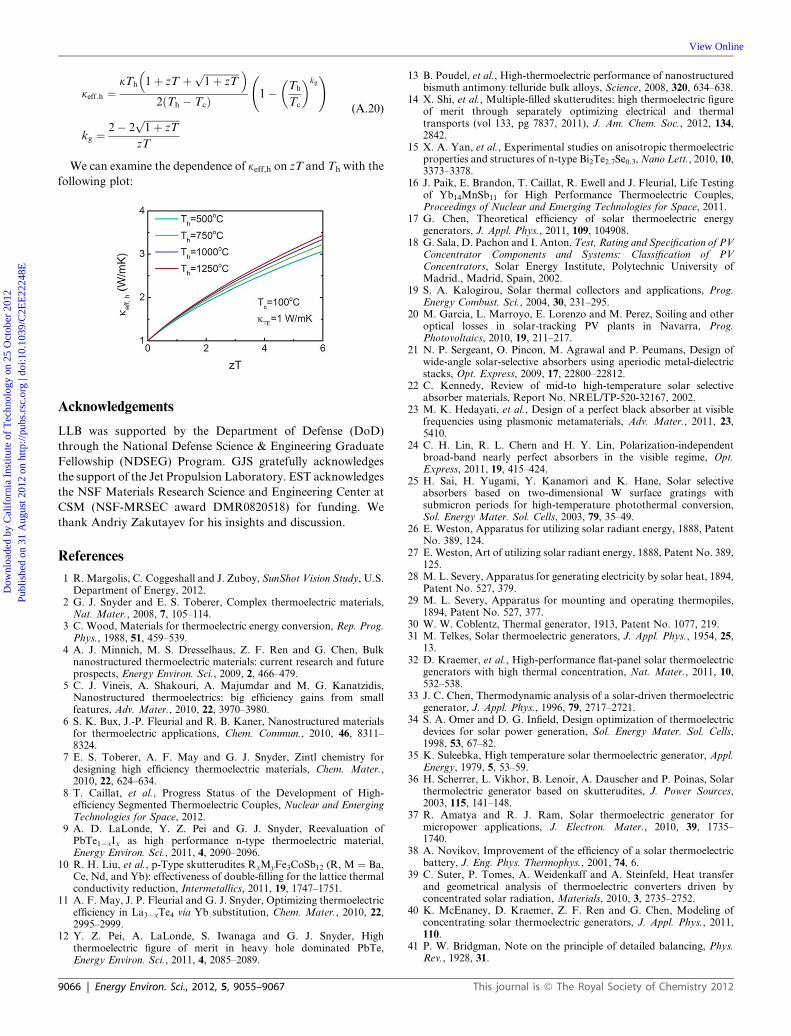
We can examine the dependence of keff,h on zT and Th with the
following plot:
Acknowledgements
LLB was supported by the Department of Defense (DoD)
through the National Defense Science & Engineering Graduate
Fellowship (NDSEG) Program. GJS gratefully acknowledges
the support of the Jet Propulsion Laboratory. EST acknowledges
the NSF Materials Research Science and Engineering Center at
CSM (NSF-MRSEC award DMR0820518) for funding. We
thank Andriy Zakutayev for his insights and discussion.
References
1 R. Margolis, C. Coggeshall and J. Zuboy, SunShot Vision Study, U.S.Department of Energy, 2012.
2 G. J. Snyder and E. S. Toberer, Complex thermoelectric materials,Nat. Mater., 2008, 7, 105–114.
3 C. Wood, Materials for thermoelectric energy conversion, Rep. Prog.Phys., 1988, 51, 459–539.
4 A. J. Minnich, M. S. Dresselhaus, Z. F. Ren and G. Chen, Bulknanostructured thermoelectric materials: current research and futureprospects, Energy Environ. Sci., 2009, 2, 466–479.
5 C. J. Vineis, A. Shakouri, A. Majumdar and M. G. Kanatzidis,Nanostructured thermoelectrics: big efficiency gains from smallfeatures, Adv. Mater., 2010, 22, 3970–3980.
6 S. K. Bux, J.-P. Fleurial and R. B. Kaner, Nanostructured materialsfor thermoelectric applications, Chem. Commun., 2010, 46, 8311–8324.
7 E. S. Toberer, A. F. May and G. J. Snyder, Zintl chemistry fordesigning high efficiency thermoelectric materials, Chem. Mater.,2010, 22, 624–634.
8 T. Caillat, et al., Progress Status of the Development of High-efficiency Segmented Thermoelectric Couples, Nuclear and EmergingTechnologies for Space, 2012.
9 A. D. LaLonde, Y. Z. Pei and G. J. Snyder, Reevaluation ofPbTe1�xIx as high performance n-type thermoelectric material,Energy Environ. Sci., 2011, 4, 2090–2096.
10 R. H. Liu, et al., p-Type skutterudites RxMyFe3CoSb12 (R, M ¼ Ba,Ce, Nd, and Yb): effectiveness of double-filling for the lattice thermalconductivity reduction, Intermetallics, 2011, 19, 1747–1751.
11 A. F. May, J. P. Fleurial and G. J. Snyder, Optimizing thermoelectricefficiency in La3�xTe4 via Yb substitution, Chem. Mater., 2010, 22,2995–2999.
12 Y. Z. Pei, A. LaLonde, S. Iwanaga and G. J. Snyder, Highthermoelectric figure of merit in heavy hole dominated PbTe,Energy Environ. Sci., 2011, 4, 2085–2089.
9066 | Energy Environ. Sci., 2012, 5, 9055–9067
13 B. Poudel, et al., High-thermoelectric performance of nanostructuredbismuth antimony telluride bulk alloys, Science, 2008, 320, 634–638.
14 X. Shi, et al., Multiple-filled skutterudites: high thermoelectric figureof merit through separately optimizing electrical and thermaltransports (vol 133, pg 7837, 2011), J. Am. Chem. Soc., 2012, 134,2842.
15 X. A. Yan, et al., Experimental studies on anisotropic thermoelectricproperties and structures of n-type Bi2Te2.7Se0.3,Nano Lett., 2010, 10,3373–3378.
16 J. Paik, E. Brandon, T. Caillat, R. Ewell and J. Fleurial, Life Testingof Yb14MnSb11 for High Performance Thermoelectric Couples,Proceedings of Nuclear and Emerging Technologies for Space, 2011.
17 G. Chen, Theoretical efficiency of solar thermoelectric energygenerators, J. Appl. Phys., 2011, 109, 104908.
18 G. Sala, D. Pachon and I. Anton, Test, Rating and Specification of PVConcentrator Components and Systems: Classification of PVConcentrators, Solar Energy Institute, Polytechnic University ofMadrid., Madrid, Spain, 2002.
19 S. A. Kalogirou, Solar thermal collectors and applications, Prog.Energy Combust. Sci., 2004, 30, 231–295.
20 M. Garcia, L. Marroyo, E. Lorenzo and M. Perez, Soiling and otheroptical losses in solar-tracking PV plants in Navarra, Prog.Photovoltaics, 2010, 19, 211–217.
21 N. P. Sergeant, O. Pincon, M. Agrawal and P. Peumans, Design ofwide-angle solar-selective absorbers using aperiodic metal-dielectricstacks, Opt. Express, 2009, 17, 22800–22812.
22 C. Kennedy, Review of mid-to high-temperature solar selectiveabsorber materials, Report No. NREL/TP-520-32167, 2002.
23 M. K. Hedayati, et al., Design of a perfect black absorber at visiblefrequencies using plasmonic metamaterials, Adv. Mater., 2011, 23,5410.
24 C. H. Lin, R. L. Chern and H. Y. Lin, Polarization-independentbroad-band nearly perfect absorbers in the visible regime, Opt.Express, 2011, 19, 415–424.
25 H. Sai, H. Yugami, Y. Kanamori and K. Hane, Solar selectiveabsorbers based on two-dimensional W surface gratings withsubmicron periods for high-temperature photothermal conversion,Sol. Energy Mater. Sol. Cells, 2003, 79, 35–49.
26 E. Weston, Apparatus for utilizing solar radiant energy, 1888, PatentNo. 389, 124.
27 E. Weston, Art of utilizing solar radiant energy, 1888, Patent No. 389,125.
28 M. L. Severy, Apparatus for generating electricity by solar heat, 1894,Patent No. 527, 379.
29 M. L. Severy, Apparatus for mounting and operating thermopiles,1894, Patent No. 527, 377.
30 W. W. Coblentz, Thermal generator, 1913, Patent No. 1077, 219.31 M. Telkes, Solar thermoelectric generators, J. Appl. Phys., 1954, 25,
13.32 D. Kraemer, et al., High-performance flat-panel solar thermoelectric
generators with high thermal concentration, Nat. Mater., 2011, 10,532–538.
33 J. C. Chen, Thermodynamic analysis of a solar-driven thermoelectricgenerator, J. Appl. Phys., 1996, 79, 2717–2721.
34 S. A. Omer and D. G. Infield, Design optimization of thermoelectricdevices for solar power generation, Sol. Energy Mater. Sol. Cells,1998, 53, 67–82.
35 K. Suleebka, High temperature solar thermoelectric generator, Appl.Energy, 1979, 5, 53–59.
36 H. Scherrer, L. Vikhor, B. Lenoir, A. Dauscher and P. Poinas, Solarthermolectric generator based on skutterudites, J. Power Sources,2003, 115, 141–148.
37 R. Amatya and R. J. Ram, Solar thermoelectric generator formicropower applications, J. Electron. Mater., 2010, 39, 1735–1740.
38 A. Novikov, Improvement of the efficiency of a solar thermoelectricbattery, J. Eng. Phys. Thermophys., 2001, 74, 6.
39 C. Suter, P. Tomes, A. Weidenkaff and A. Steinfeld, Heat transferand geometrical analysis of thermoelectric converters driven byconcentrated solar radiation, Materials, 2010, 3, 2735–2752.
40 K. McEnaney, D. Kraemer, Z. F. Ren and G. Chen, Modeling ofconcentrating solar thermoelectric generators, J. Appl. Phys., 2011,110.
41 P. W. Bridgman, Note on the principle of detailed balancing, Phys.Rev., 1928, 31.
This journal is ª The Royal Society of Chemistry 2012

Dow
nloa
ded
by C
alif
orni
a In
stitu
te o
f T
echn
olog
y on
25
Oct
ober
201
2Pu
blis
hed
on 3
1 A
ugus
t 201
2 on
http
://pu
bs.r
sc.o
rg |
doi:1
0.10
39/C
2EE
2224
8E
View Online
42 R. G. Sheppard, D.Morgan, D.M.Mathes andD. J. Bray, Propertiesand Characteristics of Graphite, Poco Graphite, Inc., 2002.
43 H. J. Goldsmid, Introduction to Thermoelectricity, Springer-Verlag,2010.
44 R. R. Heikes and R. W. Ure, Thermoelectricity: Science andEngineering, Interscience, New York, 1961.
45 G. J. Snyder, Thermoelectric Power Generation: Efficiency andCompatibility, CRC Press, Taylor & Francis Group, Boca Raton,FL, USA, 2006, ch. 9.
46 G. J. Snyder and T. S. Ursell, Thermoelectric efficiency andcompatibility, Phys. Rev. Lett., 2003, 91.
47 W. T. Xie, Y. J. Dai, R. Z.Wang andK. Sumathy, Concentrated solarenergy applications using fresnel lenses: a review, Renew. Sustain.Energ. Rev., 2011, 15, 2588–2606.
48 S. Kurtz, Opportunities and Challenges for Development of a MatureConcentrating Photovoltaic Power Industry, National RenewableEnergy Laboratories, 2011.
49 M. Peters, et al., Spectrally-selective photonic structures for PVapplications, Energies, 2010, 3, 171–193.
This journal is ª The Royal Society of Chemistry 2012
50 A. G. Imenes and D. R. Mills, Spectral beam splitting technology forincreased conversion efficiency in solar concentrating systems: areview, Sol. Energy Mater. Sol. Cells, 2004, 84, 19–69.
51 H. Hernandez-Noyola, D. H. Potterveld, R. J. Holt and S. B. Darling,Optimizing luminescent solar concentrator design, Energy Environ.Sci., 2012, 5, 5798–5802.
52 R. K. Kostuk and G. Rosenberg, Analysis and design of holographicsolar concentrators, Proc. Soc. Photo. Opt. Instrum. Eng., 2008, 7403.
53 J. D. McCambridge, et al., Compact spectrum splitting photovoltaicmodule with high efficiency, Prog. Photovoltaics, 2010, 19, 352–360.
54 S. Ruehle, et al., A two junction, four terminal photovoltaic device forenhanced light to electric power conversion using a low-cost dichroicmirror, Renewable Sustainable Energy Rev., 2009, 1.
55 J. Hernandez-Moro and J. M. Martinez-Duart, CSP electricity costevolution and grid parities based on IEA roadmaps, Energy Policy,2012, 41, 184–192.
56 K. Branker, M. J. M. Pathak and J. M. Pearce, A review of solarphotovoltaic levelized cost of electricity, Renewable SustainableEnergy Rev., 2011, 15, 4470–4482.
Energy Environ. Sci., 2012, 5, 9055–9067 | 9067