Computational Tools forMetabolic Modeling and Gene
Duplication Analysis
Stochastic Modeling and Machine Learning Approachesto Analyse the Impact of Climate Change
Pablo Spivakovsky-Gonzalez; Supervisor: Prof. Pietro Lio
Wolfson College
This thesis is submitted for the degree of Doctor of Philosophy, November 2021


Abstract
This thesis presents new computational methods to analyse both short and long-
term effects of temperature increase on biological systems. First, we consider
the problem of acclimation of an organism to increased temperatures on short
timescales. We develop a novel method of network regression, AccliNet, based
on the acclimation times, which takes into account prior knowledge of functional
links between genes to improve the performance of the algorithm. The results
obtained by AccliNet are compared with the performance of existing algorithms
and are shown to be an improvement in this area.
Next, we delve deeper into the metabolic response of the organism to chang-
ing temperatures, and develop methods to model and simulate the fluxes of
metabolites occurring through a metabolic network. In particular, we construct
a simplified model of aerobic respiration for an Antarctic species, and, given a
gene expression dataset across different temperatures, we develop two different
machine learning approaches to model the fluxes through the metabolic network.
The first approach we use is based on denoising autoencoders. The performance of
this method is compared to a traditional Bayesian inference approach and found
to have higher accuracy.
Next, we develop a different machine learning approach to model the unknown
data distributions, in this case using a Generative Adversarial Network (GAN)
to learn an SDE path through the sampled data points. The performance of
this method is compared to the earlier autoencoder approach, as well as to other
algorithms. The GAN method is found to have similar accuracy but less robustness
to noise than the autoencoder approach.
3

Lastly, we also consider the long-term effects of changing temperatures on biologi-
cal systems. In particular, we develop a novel package for phylogenetic analysis,
called PhylSim, which allows simulations and studies of adaptation and evolution
under different scenarios of climate change. We apply the package to the case of
adaptation of Antarctic species to their environment in recent evolutionary history.
The work in this thesis was carried out in collaboration with the British Antarctic
Survey, and used genetic datasets of Antarctic organisms, although the methods
developed here are general and can be readily applied to other datasets as well.
Thus, the proposed modeling framework holds some promise for tackling important
problems in the future, in areas ranging from bioinformatics to environmental
science.
Declaration
This dissertation is my own work and contains nothing which is the outcome of
work done in collaboration with others, except where specifed in the text. This
dissertation is not substantially the same as any that I have submitted for a degree
or diploma or other qualification at any other university. This dissertation does
not exceed the prescribed limit of 60,000 words.
Pablo Spivakovsky-Gonzalez
November 30, 2021

Acknowledgements
First and foremost, I wish to thank my supervisor, Professor Pietro Lio, for
his guidance and support throughout the entire PhD - even in the most difficult
times, such as the coronavirus pandemic. Without him, none of the research done
for this PhD would have been possible!
I also wish to thank our collaborators at the British Antarctic Survey, Pro-
fessor Melody Clark and Professor Lloyd Peck, for their help on the biology
side, especially in the interpretation of biological data and explaining the specific
adaptations of Antarctic organisms to their environment. Also a big thank you to
Dr. Alessandro Di Stefano and Dr. Thomas Sauerwald for their helpful comments
and suggestions regarding the thesis!
Next, I wish to thank the department and my college (Wolfson) for their support
during the COVID-19 pandemic and period of medical intermission. A special
thank you also to Lise Gough, whose help on the administrative side has been
crucial throughout the entire PhD!
Lastly, I wish to thank the Natural Environment Research Council (NERC)
for funding this PhD as part of the DREAM Centre for Doctoral Training in Big
Data, Risk and Environmental Analytical Methods; NERC covered tuition and
college fees for the duration of the programme. And of course a huge thank you to
my family and friends for all their support and encouragement from the beginning
of the PhD until now,
Pablo Spivakovsky-Gonzalez
PhD Candidate

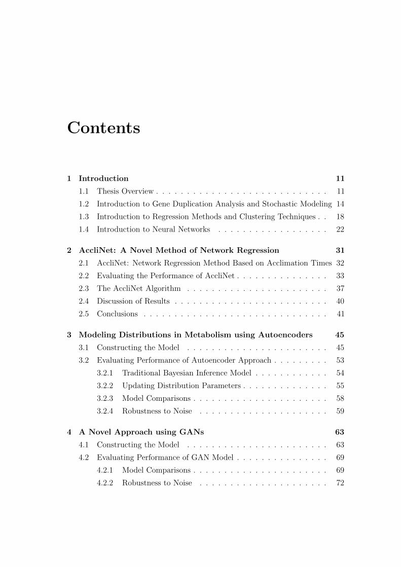
Contents
1 Introduction 11
1.1 Thesis Overview . . . . . . . . . . . . . . . . . . . . . . . . . . . . 11
1.2 Introduction to Gene Duplication Analysis and Stochastic Modeling 14
1.3 Introduction to Regression Methods and Clustering Techniques . . 18
1.4 Introduction to Neural Networks . . . . . . . . . . . . . . . . . . 22
2 AccliNet: A Novel Method of Network Regression 31
2.1 AccliNet: Network Regression Method Based on Acclimation Times 32
2.2 Evaluating the Performance of AccliNet . . . . . . . . . . . . . . . 33
2.3 The AccliNet Algorithm . . . . . . . . . . . . . . . . . . . . . . . 37
2.4 Discussion of Results . . . . . . . . . . . . . . . . . . . . . . . . . 40
2.5 Conclusions . . . . . . . . . . . . . . . . . . . . . . . . . . . . . . 41
3 Modeling Distributions in Metabolism using Autoencoders 45
3.1 Constructing the Model . . . . . . . . . . . . . . . . . . . . . . . 45
3.2 Evaluating Performance of Autoencoder Approach . . . . . . . . . 53
3.2.1 Traditional Bayesian Inference Model . . . . . . . . . . . . 54
3.2.2 Updating Distribution Parameters . . . . . . . . . . . . . . 55
3.2.3 Model Comparisons . . . . . . . . . . . . . . . . . . . . . . 58
3.2.4 Robustness to Noise . . . . . . . . . . . . . . . . . . . . . 59
4 A Novel Approach using GANs 63
4.1 Constructing the Model . . . . . . . . . . . . . . . . . . . . . . . 63
4.2 Evaluating Performance of GAN Model . . . . . . . . . . . . . . . 69
4.2.1 Model Comparisons . . . . . . . . . . . . . . . . . . . . . . 69
4.2.2 Robustness to Noise . . . . . . . . . . . . . . . . . . . . . 72

5 The PhylSim Package 75
5.1 Simulation of An Adaptive Radiation . . . . . . . . . . . . . . . . 78
5.2 Multivariate Simulation . . . . . . . . . . . . . . . . . . . . . . . 81
5.3 Parameter Estimation . . . . . . . . . . . . . . . . . . . . . . . . 82
5.4 Directions for Future Work . . . . . . . . . . . . . . . . . . . . . . 84
6 Conclusions 87

9

10

Chapter 1
Introduction
1.1 Thesis Overview
Global climate change is one of the main challenges facing our society in the
21st century. As indicated in the latest report by the Intergovernmental Panel
on Climate Change (IPCC)[1], mean annual temperatures have risen by more
than one degree Celsius in the last century, and are expected to rise an additional
1.5 degrees by the end of this century, if current trends continue. This increase
in temperature will likely have far-reaching consequences, both for the natural
environment and for human activities. Some of the most immediate consequences
that can be foreseen are the melting of polar ice, with the consequent rise in
global sea levels; the expansion of deserts in the interior of the continents; and
the occurrence of more frequent and more extreme weather events throughout the
globe [1].
However, the rise in global surface temperatures will not be homogeneous. In
light of current trends, it is believed that the polar regions may warm at twice the
rate of the temperate zones [1]. This disproportionate temperature increase will
likely upset the balance of many polar ecosystems, as the flora and fauna in these
regions have adapted over millions of years to live in a very narrow temperature
range, with all metabolic functions optimised for stable existence in the extreme
cold.
Although many of these adaptations to the polar environment remain poorly
11

understood, in recent years scientists have obtained a wealth of genomic and
transcriptomic data that can shed some light in this area. However, there is
currently a lack of suitable algorithms to analyse and interpret the vast amounts
of biological data that have been obtained.
Fortunately, recent advances in machine learning and stochastic modeling may
hold the key to developing effective models that will allow correct analysis, inter-
pretation and prediction from existing data. In particular, methods such as neural
networks, stochastic differential equations, and network regression can be applied
to current datasets in order to understand the effects of rising temperatures on
biological organisms.
This thesis presents new computational methods to analyse both short and
long-term effects of temperature increase on biological systems. The work is
carried out in collaboration with the British Antarctic Survey, and uses genetic
datasets of Antarctic organisms, although the methods developed here are general
and can be readily applied to other datasets as well.
This work is organised as follows. In the current chapter, we present the necessary
background information that will serve as a foundation for later chapters.
In Chapter 2, we consider the problem of acclimation of an organism to increased
temperatures on short timescales. Given a gene expression dataset for different
tissues and a set of acclimation times, we wish to determine which genes (or sets of
genes) are most significant in the acclimation response for each tissue. With this
in mind, we develop a novel method of network regression, AccliNet, based on
the acclimation times, which takes into account prior knowledge of functional links
between genes to improve the performance of the algorithm. The results obtained
by AccliNet are compared with the performance of existing algorithms in this area.
In Chapters 3 and 4, we delve deeper into the metabolic response of the
organism to changing temperatures, and develop methods to model and simulate
the fluxes of metabolites occurring through a metabolic network. In particular,
we construct a simplified model of aerobic respiration for an Antarctic species,
and, given a gene expression dataset across different temperatures, we develop two
12

different machine learning approaches to model the fluxes through the metabolic
network.
In Chapter 3, the approach we use is based on denoising autoencoders, which are
used to alternately add and remove noise from the sampled data to construct a
Markov chain that can then be shown over time to approximate the true data dis-
tribution [2]. The performance of this method is compared to traditional Bayesian
inference approaches, as well as to other existing algorithms. In Chapter 4,
Figure 1.1: A visual overview of the main chapters of the thesis.
we develop a different machine learning approach to model the unknown data
distributions, in this case using a Generative Adversarial Network (GAN) to learn
an SDE path through the sampled data points (here, the term “SDE” refers to
“stochastic differential equation”). The performance of this method is compared to
the method presented in Chapter 3, as well as to traditional Bayesian inference
approaches and other algorithms, in terms of robustness, accuracy, etc.
13

In Chapter 5, we consider the long-term effects of changing temperatures on
biological systems. In particular, we develop a novel package for phylogenetic
analysis, called PhylSim, which allows simulations and studies of adaptation
and evolution under different scenarios of climate change. We apply the package
to the case of adaptation of Antarctic species to their environment in recent
evolutionary history. A recent publication related to this work can be found here:
https://doi.org/10.1101/2020.05.13.094706
A visual overview of the thesis is given in Figure 1.1. Finally, Chapter 6
will summarise the results of the thesis. We now introduce some of the necessary
background that will be used in subsequent chapters of the thesis.
1.2 Introduction to Gene Duplication Analysis
and Stochastic Modeling
An in-depth genetic analysis provides important clues to an organism’s metabolic
functions. In particular, protein-coding genes determine the amino acid sequences
that make up each metabolic enzyme, which in turn determines that enzyme’s
structure. The structure then influences how the enzyme interacts with other
compounds. In most metabolic processes, enzymes play a crucial role in acting
as catalysts between products and reactants. Thus, the production of sufficient
quantities of an enzyme is key in setting reaction rates in metabolic networks [4].
The study of the genes that code for each enzyme, as well as those genes with
regulatory functions, can also reveal instances of metabolic adaptation in an
organism. An important mechanism for adaptation is gene duplication, which
occurs when an extra copy of a gene is produced in the genome. The presence of
this additional copy can augment gene function, and for example lead to increased
production of a particular enzyme.
This can give an organism a comparative advantage when adapting to its environ-
ment, in which case the extra copy will likely be retained and spread throughout
the population. On the contrary, if the extra copy is not beneficial to the organ-
14

ism’s survival, then it will typically be removed from the population over the
course of generations, due to natural selection against that genetic change [5].
As a result of this, metabolic genes that have undergone successive duplica-
tions on a relatively short time scale are a strong indication of metabolic pathways
important for adaptation. In the case of Antarctic fish species, for example,
some metabolic genes are present in four or five copies, while related species
inhabiting warmer waters only possess a single copy. Hence, we can use analysis
of gene duplications to identify metabolic pathways of particular interest prior to
computational modeling.
Gene duplications can be modelled as a stochastic birth-death process evolv-
ing over a species tree (also called a phylogeny) [6]. Moreover, we can consider
the number of copies of each gene as a specific trait evolving on the phylogeny.
This allows comparison of different branches of the tree to determine how the
number of gene copies evolves between species, and across groups of related species.
In particular, the number of gene copies actually observed in each species can be
compared to the predicted distribution of gene copies assuming random dupli-
cations and genetic drift over time. This analysis would help to identify which
metabolic genes are under positive selection (preferentially duplicated and retained
over time) in each branch of the species tree, as compared to a model of gene
duplications occurring at random without any selection.
In the field of quantitative genetics, this multivariate adaptation is seen as occur-
ring by small allele shifts happening simultaneously at many loci; see for example
Barton et al. (2002) [7]. Classical population genetics, on the other hand, envisions
multivariate adaptation as a series of large shifts, each occurring independently at
single loci; see Pritchard et al. (2010) [8], for instance.
In the limit, the first approach leads to the “infinitesimal” model of evolution, in
which adaptation happens gradually by infinitesimal changes occurring together
over many loci [9]. The second approach leads to the “sweep” model, in which
adaptation happens through large changes at particular loci, each having a rapid
impact on the value of the trait [10]. In recent years, several studies have tried
15
to combine the two approaches into a unified theory, such as Boyle et al. (2017) [11].
One model that has received considerable attention is that of “punctuated equilib-
rium” [12]. In this model, adaptation happens rapidly at the time of speciation by
a large jump in the value of the trait, but only very gradually between speciation
events, which results in long periods of relative stasis. As indicated by Bokma
(2010) [13], the theory of punctuated equilibrium would agree to some extent with
the fossil record, where scientists rarely observe gradually changing lifeforms, but
rather distinct species occurring with long periods of stasis between them.
Models considering both gradual and punctuated evolution have been discussed
by Mooers at al. (2012) [14], and Mattila and Bokma (2008) [15] for example.
However, when fitting these models to data, it is often difficult to separate the
two components based only on extant species, due to estimation error and to the
multiple sources of stochasticity occurring over long timescales.
On time scales of microevolution, quantitative genetics has been successful to
some extent in modeling adaptation as variations in multiple traits occurring
along a static adaptive landscape [16]. However, more recent work has shown
that adaptation on macroevolutionary timescales happens rather through changes
in the structure of the adaptive landscape itself [17], in particular by shifts in
adaptive peaks of the different traits [18].
Early phylogenetic comparative methods that attempted to capture the dynamics
of multivariate adaptation used multivariate Brownian motion processes [19], and
as a result were unable to consider adaptation of traits toward optima that could
shift over time. For univariate traits, the case of shifting optima was considered by
Butler and King (2004) [20]. In this work, the authors modeled random evolution
of traits using an Ornstein-Uhlenbeck diffusion process occuring on a species tree
over time. Their implementation resulted in the OUCH package [20].
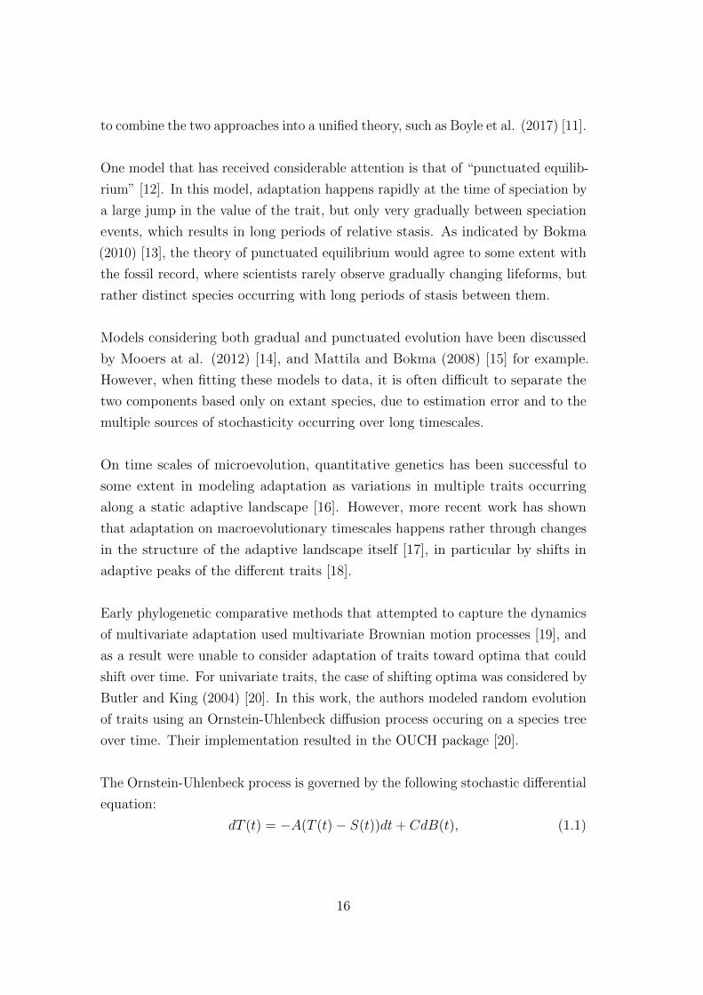
The Ornstein-Uhlenbeck process is governed by the following stochastic differential
equation:
dT (t) = −A(T (t)− S(t))dt+ CdB(t), (1.1)
16

where T (t) is the value of the trait at time t, A is the genetic drift term, B(t) is a
standard Brownian motion, S(t) is some theoretically optimal trait distribution
to which the process tends, and C is a stochastic diffusion term [13].
The solution to the above differential equation is of the form
T (t) = exp(−At)T (0) +
∫ t
0
exp(−A(t− τ))AS(t)dτ +
∫ t
0
exp(−A(t− τ))CdB(τ).
(1.2)
The OUCH package allowed a limited multivariate model of shifting optima for
the special case when the drift matrix of the traits was symmetric positive definite.
Hansen et al. (2008) [21] expanded this with the SLOUCH package, which
allowed models of multivariate adaptation to changing peaks for a certain range
of parameters. Roper et al. (2008) [22] also considered cases of bivariate Ornstein-
Uhlenbeck processes, but again with important restrictions on the set of parameters
that could be employed.
Bartoszek et al. (2012) [23] then extended the SLOUCH package to consider a
wider range of scenarios involving multiple traits evolving together on the species
tree. Hence, T (t) becomes ~T (t), that is, a vector of trait values at time t, and the
stochastic differential equation for the Ornstein-Uhlenbeck process becomes
d~T (t) = −A(~T (t)− ~S(t))dt+ Cd ~B(t), (1.3)
with A and C now as matrices acting on the corresponding vectors [14].
The solution for the multivariate case is therefore
~T (t) = exp(−At)~T (0)+
∫ t
0
exp(−A(t−τ))A~S(t)dτ+
∫ t
0
exp(−A(t−τ))Cd ~B(τ).
(1.4)
The power of this multivariate approach is that it can consider more interactions
occurring between multiple traits evolving simultaneously toward shifting optima.
In particular, a vector of trait values ~T (t) can be subdivided into two trait vectors,~X(t) and ~Y (t), representing “effect” and “response” traits, to model different
types of trait interactions; for example, cases of co-adaptation between traits, or
17

some traits responding to the effects of others. This approach was implemented in
the mvSLOUCH package [23], which allowed greater flexibility than the SLOUCH
package for testing evolutionary hypotheses over a phylogeny.
The mvSLOUCH framework was further improved by Bartoszek and Lio (2019)
[24] with the ‘pcmabc’ package. This package uses Approximate Bayesian Com-
putation (ABC) to fit parameters of the stochastic process, thereby making the
computation more efficient. The Approximate Bayesian Computation method
allows posterior distributions of model parameters to be estimated without the
need to evaluate the likelihood function, which is often computationally challeng-
ing [24]. The ‘pcmabc’ package also relies on the ‘yuima’ package [25] for solving
SDEs more robustly.
Both the mvSLOUCH and ‘pcmabc’ packages allow the user to simulate trait
evolution on a phylogeny under a particular evolutionary model and speciation
rate. In the case of the ‘pcmabc’ package, even switching between rates is allowed
by the simulation. However, neither package allows the user to specify a large
number of regimes, with different evolutionary models and speciation rates for
each regime. This additional functionality is provided by the PhylSim package,
presented in Chapter 5.
1.3 Introduction to Regression Methods and Clus-
tering Techniques
In recent years, there has been a significant increase in the amount of genomic
and transcriptomic data available to study Antarctic organisms. However, the
interpretation of high-dimensional gene expression data has been hindered by a
lack of suitable algorithms in this area. In an attempt to address this problem,
Thorne et al. (2010) [50] used a hierarchical clustering algorithm based on Eu-
clidean distance to cluster differentially expressed genes.
In hierarchical clustering, a recursive procedure is used to separate data into
different clusters by constructing a hierarchy. This hierarchy can be obtained by a
divisive algorithm, in which the data is first grouped into a single cluster, and then
18
divided recursively into smaller clusters, based on a dissimilarity measure; the
other alternative is to use an agglomerative approach, in which each data point
is initially treated as a cluster, and separate clusters are then merged together
recursively if they contain similar data points [51].
Apart from hierarchical clustering, another approach that has been frequently
used is K-means clustering [52]. In the K-means algorithm, cluster memberships
are updated iteratively in order to obtain the minimum sum of distances between
each data point and the centroid of its cluster. Thus, the algorithm solves the
optimization problem
(C∗,m1∗, ...,mn
∗) = arg minC,m1,...,mn
∑C(i)=j
||pi −mj ||2. (1.5)
The optimal mj is simply the “centre of mass” of the data in the j-th cluster [52].
Then the optimal cluster membership for the i-th data point is given by
C(i) = arg minj||pi −mj||2. (1.6)
The K-means algorithm uses alternating minimization, but note however that
the process may converge on local rather than global minima. As a result, it is
recommended to try multiple initial values to avoid this problem.
Another clustering approach, known as supervised group Lasso (SGLasso), has
been used by Ma et al. (2007) [53]; in this method, important genes within each
cluster were first identified using a Lasso model, and then the most significant
clusters were selected using group Lasso. Simon et al. (2012) [54] later improved
upon this method by combining Lasso Cox regression with a group Lasso con-
straint.
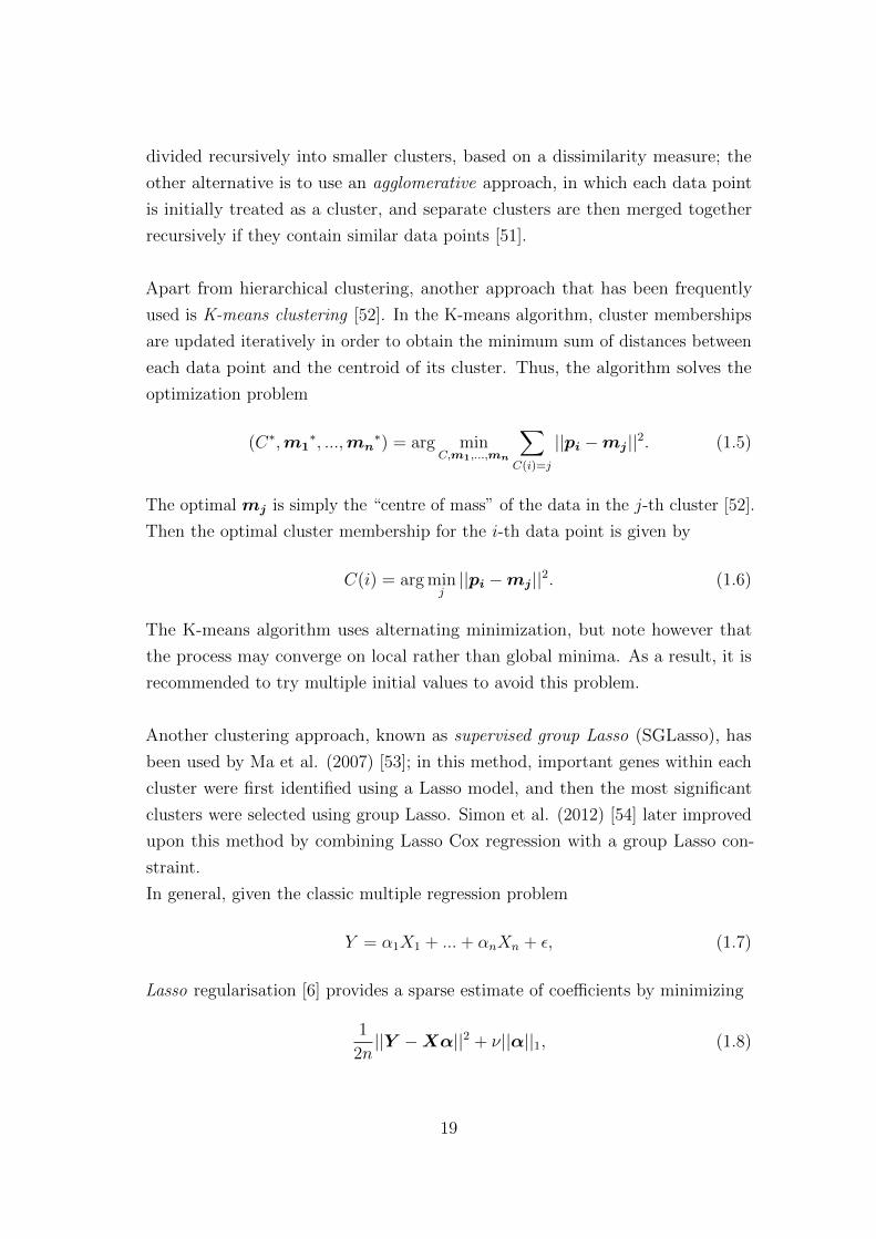
In general, given the classic multiple regression problem
Y = α1X1 + ...+ αnXn + ε, (1.7)
Lasso regularisation [6] provides a sparse estimate of coefficients by minimizing
1
2n||Y −Xα||2 + ν||α||1, (1.8)
19

where the second term corresponds to the L1-norm, and ν is an adjustable param-
eter. Although the Lasso method is useful in some situations for dealing with the
high dimensionality problem, the main drawback is the bias resulting from large
coefficients [55].
To deal with this problem, Zou (2006) [56] suggested the method of adaptive
Lasso, in which a set of adaptive weights are added to the L1 penalty. Then the
regression coeffficients are estimated by minimizing
1
2n||Y −Xα||2 + ν
n∑i=1
wi|αi|1, (1.9)
where wi are the adaptive weights that compensate for the bias resulting from
large coefficients. Note that the wi must be non-negative to maintain convexity of
the Lasso model [56].
Other algorithms have instead used a ridge penalty, which also penalizes large
coefficients to prevent overfitting on a given sample size [57]. In ridge regression,
the coefficients are estimated by minimizing
1
2n||Y −Xα||2 + ν
n∑i=1
|αi|2, (1.10)
which is equivalent to the least-squares estimate with an L2 penalty [57].
To combine the benefits of both Lasso and ridge regression, Zou and Hastie (2005)
[58] proposed the Elastic Net algorithm, which estimates coefficients by minimizing
1
2n||Y −Xα||2 + ν1||α||1 + ν2||α||2, (1.11)
and thus incorporates both an L1 and an L2 penalty. The Elastic Net reduces
to pure Lasso when ν2 = 0, and pure ridge regression when ν1 = 0. In general,
Elastic Net maintains sparsity of the Lasso due to the L1 penalty, and is also able
to handle highly correlated covariates due to the L2 penalty [58].
Other methods for studying high-dimensional datasets have relied on classi-
fication trees for estimation of coefficients and making predictions. A classification
20

tree is generally built by recursively partitioning the predictor space into different
regions, so that the final regions correspond to the terminals of a decision tree
[51].
Although classification trees are convenient for certain datasets, the main draw-
back is the high degree of variability, as slightly different training data can lead to
large differences in the resulting decision tree. One method to reduce this problem
is bagging (bootstrap aggregating) [59].
In this approach, multiple decision trees are constructed from the training data by
“bootstrapping”, ie. taking repeated samples with replacement from the dataset.
The bagging estimator then takes an average of the estimates produced by all the
different trees to produce a final, aggregate estimate [59].
An improvement on the bagging approach is the method of random forests [60].
In this method, in addition to using a bootstrap sample, each decision tree is
constructed using a random subset of the predictors, which reduces artificial
correlations between the trees. The final estimate is again an average of the
estimates produced by all the different decision trees [60].
Although useful for some analyses, methods such as Lasso, ridge regression or clas-
sification trees are purely statistical, and as a result do not allow the incorporation
of prior information about gene associations or gene networks into the regression
algorithm. Other approaches for studying high-dimensional datasets have relied
on first transforming the data into a related component space of lower dimension,
for example using principal component analysis (PCA), before performing the
regression [61].
The transformation to principal components is an orthogonal coordinate change
that concentrates most of the variance in the data in the first principal component,
then most of the remaining variance in the second principal component, and so
on [61]. Consider a data matrix Y with n columns. Then the transformation is
defined by a set of n-dimensional vectors of weights g = (g1, ..., gn) that map each
row vector y of Y to a vector of principal component scores r = (r1, ..., rn), such
21

that
r = g · y, (1.12)
with the weight vector g constrained to be of unit length, and with the individual
variables of r successively inheriting the maximum possible variance from y.
The principal components are orthogonal to each other, and usually the first
few components are enough to capture almost all the variance of the data set,
regardless of high dimensionality in the original data. Hence, principal components
have become a popular method for dimensionality reduction of large data sets in
many disciplines [62].
Bilyk and Cheng (2014) [63] used a multidimensional scaling algorithm based on
PCA to analyse differential gene expression of Pagothenia borchgrevinki under
heat stress. This approach was expanded in Bilyk et al. (2018) [64], with the use
of a Generalized Linear Model (GLM) to analyse gene expression after performing
the multidimensional scaling.
Although these methods were able to reduce the dimensionality of the data
and identify some important genes, they could not incorporate prior information
about gene networks into the analysis, and thus had to rely solely on statistical
correlations between genes, without considering functional linkage or gene sig-
naling. Hence, despite the important insights gained in these studies, many of
the underlying mechanisms that allow acclimation and adaptation to changing
conditions are still not well understood.
1.4 Introduction to Neural Networks
In simple terms, neural networks provide a way to approximate high-dimensional
functions by composing linear transformations and using nonlinear gating. The
family of functions generated in this way is very flexible and thus allows good
approximations of most target functions.
Although neural networks have been around for some time, recent advances
in computation have led to great advances in their performance. Today, neural
22

nets are used successfully in such difficult tasks as machine translation, computer
vision or natural language processing, where the information set is complex and
there is a high signal-to-noise ratio.
The use of big data allows the reduction of variance in deep neural networks, and
new architectures permit the construction of deeper networks which give better
approximations of high-dimensional functions. The result is a set of scalable meth-
ods that are very successful in high-dimensional function estimation in situations
with a large sample size.
Formally, given a training dataset (xi, yi) where yi ∈ Rd is the output and
xi ∈ R is the input, we wish to find a function g : Rd → R that will perform
well in making predictions from test data. Statisticians and computer scientists
have worked for decades on methods for finding g effectively in a variety of settings.
In neural networks, g is obtained from the compositional function class
g(x; θ) = Mkσk(Mk−1 · · · σ1(M1x + b1) + bk−1) + bk), (1.13)
where the parameters θ = {M1, ...,Mk,b1, ...,bk} are matrices {Mj} and vectors
{bj} of appropriate size. Here, for each j, σj is a nonlinear function, called an
activation function that is applied to each component of the inputs from the
previous layer. Thus, we start from x(0) = x, and recursively compute
x(j) = σj(Mjx(j−1) + bj), (1.14)
and
g(x; θ) = x(k). (1.15)
We now introduce some terminology. The input xi is often referred to as the
feature, the output yi as the label, and the pair (xi, yi) as an example.
In classification problems, the function g is referred to as the classifier, and
the process of estimating g is known as training. To evaluate the performance of
g, the most common approach is to use the prediction error, that is, P (y 6= g(x)),
often using a separate dataset for evaluation. The learning process consists pri-
23
marily in estimating parameters θ of the function g.
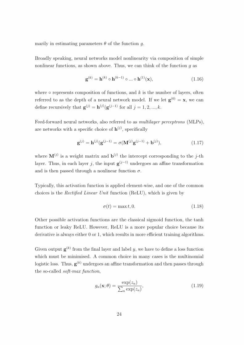
Broadly speaking, neural networks model nonlinearity via composition of simple
nonlinear functions, as shown above. Thus, we can think of the function g as
g(k) = h(k) ◦ h(k−1) ◦ ... ◦ h(1)(x), (1.16)
where ◦ represents composition of functions, and k is the number of layers, often
referred to as the depth of a neural network model. If we let g(0) = x, we can
define recursively that g(j) = h(j)(g(j−1) for all j = 1, 2, ..., k.
Feed-forward neural networks, also referred to as multilayer perceptrons (MLPs),
are networks with a specific choice of h(j), specifically
g(j) = h(j)(g(j−1) = σ(M(j)g(j−1) + b(j)), (1.17)
where M(j) is a weight matrix and b(j) the intercept corresponding to the j-th
layer. Thus, in each layer j, the input g(j−1) undergoes an affine transformation
and is then passed through a nonlinear function σ.
Typically, this activation function is applied element-wise, and one of the common
choices is the Rectified Linear Unit function (ReLU), which is given by
σ(t) = max t, 0. (1.18)
Other possible activation functions are the classical sigmoid function, the tanh
function or leaky ReLU. However, ReLU is a more popular choice because its
derivative is always either 0 or 1, which results in more efficient training algorithms.
Given output g(k) from the final layer and label y, we have to define a loss function
which must be minimised. A common choice in many cases is the multinomial
logistic loss. Thus, g(k) undergoes an affine transformation and then passes through
the so-called soft-max function,
gn(x; θ) =exp(zn)∑n exp(zn)
, (1.19)
24
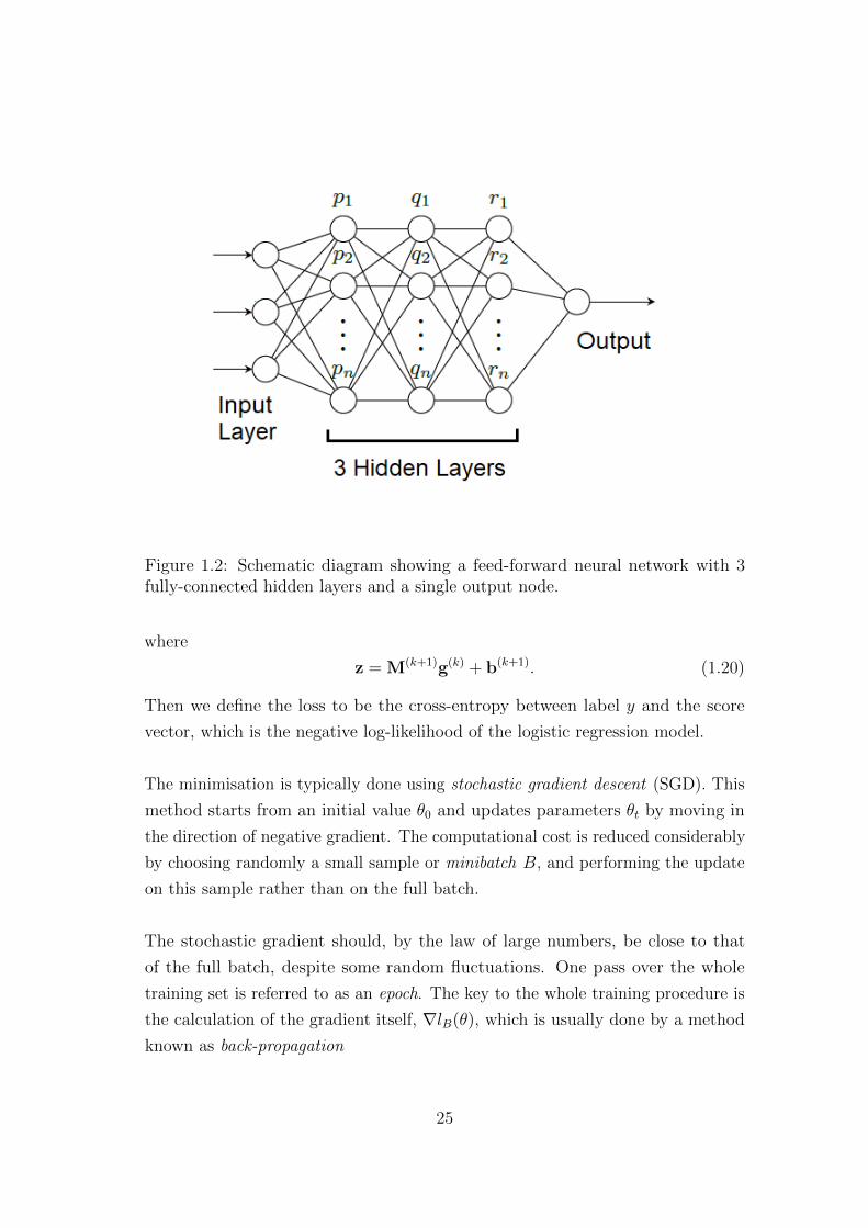
Figure 1.2: Schematic diagram showing a feed-forward neural network with 3fully-connected hidden layers and a single output node.
where
z = M(k+1)g(k) + b(k+1). (1.20)
Then we define the loss to be the cross-entropy between label y and the score
vector, which is the negative log-likelihood of the logistic regression model.
The minimisation is typically done using stochastic gradient descent (SGD). This
method starts from an initial value θ0 and updates parameters θt by moving in
the direction of negative gradient. The computational cost is reduced considerably
by choosing randomly a small sample or minibatch B, and performing the update
on this sample rather than on the full batch.
The stochastic gradient should, by the law of large numbers, be close to that
of the full batch, despite some random fluctuations. One pass over the whole
training set is referred to as an epoch. The key to the whole training procedure is
the calculation of the gradient itself, ∇lB(θ), which is usually done by a method
known as back-propagation
25

Back-propagation is based on applying the chain rule for calculating deriva-
tives of function compositions in networks. The calculation can be thought of as
occurring in a backward fashion. First, we calculate ∂lB∂g(k)
, then ∂lB∂g(k−1) , and so on,
until reaching ∂lB∂g(1)
.
Thus, we obtain the following recursive relation:
∂lB∂g(j−1)
=∂g(j)
∂g(j−1)· ∂lB∂g(j)
, (1.21)
where the computation of ∂lB∂g(j−1) is dependent on ∂lB
∂g(j). In that sense, the deriva-
tives are propagated backward starting from the last layer and moving towards
the first. These derivatives are used in updating the parameters.
For example, the gradient update for M(j) is calculated as
M(j) ←M(j) − γ ∂lB
∂M(j), (1.22)
where the step size γ is positive and is referred to as the learning rate. The
learning rate determines how much the parameters can be changed during each
update.
Apart from standard feed-forward neural networks, two other popular models are
recurrent neural networks (RNNs) and convolutional neural networks (CNNs).
These two models share an important characteristic, which is weight sharing.
Weight sharing refers to the fact that in recurrent neural nets some parameters
are identical across time, while in convolutional neural nets they are identical
across locations.
Convolutional neural networks are a specific kind of feed-forward neural networks
used extensively in image processing. CNNs are made of two types of components,
convolutional layers and pooling layers. In the convolutional layer, the input
feature undergoes first an affine transformation and then nonlinear activation.
However, during the affine transformation, a number of filters are applied to extract
features from the input of the previous layer. The pooling layer on the other hand
26

combines the information of neighbouring features into one to reduce computation.
Recurrent neural networks on the other hand are especially well-suited for pro-
cessing sequential data. RNNs have been used successfully in applications such
as machine translation or speech recognition. They can also be combined with
convolutional neural networks to create more complex models.
We now turn to unsupervised learning models using neural networks. There
are two types of models that have become increasingly popular in recent years:
autoencoders and generative adversarial networks (GANs). Autoencoders can
be regarded in some sense as a dimension reduction technique, while generative
adversarial networks are more akin to a probability density estimation method.
We will look first at autoencoders. As in any method of dimension reduction, the
goal is to preserve the main features of the data while reducing the dimensionality.
An autoencoder consists of two main components, an encoder function g that
maps an input x ∈ Rd to a hidden representation h = g(x) ∈ Rk, and a decoder
function f that maps h back to f(h) ∈ Rd.
Both the encoder and decoder may be multilayer neural networks. Now let
L(xi,xj) be the loss function which measures the distance between xi and xj) in
Rd. An autoencoder attempts to find encoder g and decoder f that minimises
the value of L(x, f(g(x)).
This goal corresponds to solving the minimisation problem
minf,g
1
n
n∑i=1
L(xi, f(g(xi))). (1.23)
To avoid trivial solutions, we can impose structural assumptions on f and g, such
as requiring that the encoder maps to a lower dimensional space, i.e. k strictly
less than d. A schematic diagram of an autoencoder is shown in Figure 1.3. A
variety of different autoencoders have been developed suited to various tasks. One
example is that of denoising autoencoders. A denoising autoencoder replaces xi
27

Figure 1.3: Schematic diagram showing an example of an autoencoder with theencoder on the left and decoder on the right. [52]
with a corrupted version x’i by adding a small amount of noise ηi,
x’i = xi + ηi. (1.24)
Thus, L(xi, f(hi)) becomes L(xi, f(g(x’i))). When minimising this loss function,
the result is that the encoder and decoder are robust to small perturbations in
the data.
A different approach to unsupervised learning is that of generative adversar-
ial networks (GANs). A GAN learns through a competitive process involving two
players, one referred to as the generator and the other as the critic or discrimi-
nator. The generator attempts to produce synthetic samples imitating the true
distribution, and the critic tries to discern whether the sample produced is real
or synthetic. The competition between the two players drives the process and
28

improves the performance of the GAN over time.
More formally, the generator is made up of two components, a source distri-
bution PZ and a function f that maps a sample from PZ to another point f(Z)
which is in the same space as x. In this case, f(Z) is a synthetic sample produced
by the generator.
The discriminator on the other hand consists of a function that takes an in-
put x, synthetic or real, and returns the probability that x is a real sample
from PX . Thus, the discriminator returns a value on the interval [0, 1]. The
payoff is higher for the discriminator if it is able to distinguish between real and
synthetic samples, and the payoff is higher for the generator if it is able to fool the
discriminator. Let θf and θd be the parameters of functions f and d respectively.
Figure 1.4: Schematic diagram showing an example of a generative adversarialnetwork (GAN). [52]
Then the GAN attempts to solve the min-max problem
minθf
maxθd
Ex∼PX [log(d(x))] + Ez∼PZ [1− log(d(f(Z)))] (1.25)
29

If we fix the parameters θf of the generator, the discriminator’s goal is to solve
the inner maximisation problem. On the other hand, if we fix the parameters θd
of the discriminator, the generator attempts to produce more realistic samples
f(Z). A schematic diagram of a GAN is shown in Figure 1.4.
We thus conclude the necessary background material for this work. In the
following chapter, we will consider the problem of acclimation of an organism to
increased temperatures on short timescales, and develop a new method of network
regression called AccliNet to study this problem.
30

Chapter 2
AccliNet: A Novel Method of
Network Regression
In this chapter, we present a regression method called AccliNet that utilizes gene
expression data from different tissues and known acclimation times, and incorpo-
rates prior knowledge of functional links between genes into the regression, in order
to determine with greater accuracy which genes and subnetworks are most relevant
to acclimation across different tissues. Previous work on network-based regression
has been done in other areas, for example in biomedical applications. Zhang et al.
(2013) [65] used prior knowledge of gene networks in their regression algorithm to
detect signature genes for survival in cancer treatments. More recently, Iuliano et
al. (2018) [66] combined network-based regression with screening algorithms for
survival analysis in the case of breast cancer.
However, as far as we are aware, AccliNet is the first network regression method
based on the acclimation times, and thus presents a completely new approach to
the analysis of gene expression data. It is also the first use of network regression
specifically in the study of Antarctic organisms. As a result, an approach that
takes into account network constraints can shed new light on the underlying
mechansims that allow acclimation to changing conditions in these organisms.
31

2.1 AccliNet: Network Regression Method Based
on Acclimation Times
Let D be the gene expression profile of k specimens over n genes. Then the
probability of acclimation at time t for the i-th specimen with expression profiles
D i = (D1, ..., Dn) is given by
p(t | D i) = p0(t)exp(D′iα) (2.1)
where p0(t) is a baseline function and α = (α1, ..., αn) is a vector of regression co-
efficients. In classical Cox regression, the coefficients are estimated by maximizing
the log-partial likelihood:
l(α) =k∑i=1
δi
D ′iα− log ∑m∈R(ti)
exp(D ′mα)
(2.2)
where ti is the acclimation time for the i-th specimen, and δi is an indicator of
whether the time is observed (δi = 1) or censored (δi = 0) [65]. To estimate p0(t),
we use
p0(t) = 1/∑
m∈R(ti)
exp(D ′mα), (2.3)
known as a Breslow estimator [67]. Then the total log-likelihood is given by
L(α, p0) =k∑i=1
δi[log(p0(ti)) + D ′iα]− exp(D ′iα)∑tj<ti
p0(tj)
(2.4)
The regression coefficients α are estimated by maximizing the total log-likelihood.
This is done by alternating between maximizing with respect to p0(t) (using the
Breslow estimator) and with respect to α, by the Newton-Raphson method [65].
Next, we wish to incorporate into the model the information derived from network
constraints. For this purpose, we represent functional links between genes using a
graph representation G, in which each node represents a gene, and there is an
edge between two nodes if and only if there is a known functional link between
those genes. The edges are weighted according to the strength of the link between
the genes, in order to encourage assigning similar regression coefficients to genes
32

connected by edges with large weights. The link strength between genes is given
by the functional linkage network obtained from the MetaFishNet project [27].
More formally, let W be the weight matrix for the graph G. We define a cost
function C1(α) as follows:
C1(α) =1
2
n∑i,j=1
Wi,j(αi − αj)2 =1
2α′(I−W)α =
1
2α′Λα, (2.5)
where I is the identity matrix and Λ is the Laplacian. This function penalizes
having large differences between the regression coefficients assigned to closely
related genes (nodes linked by a highly weighted edge). In addition, we incorporate
an L2-norm constraint to avoid very large coefficients, which can be unreliable
[67]. The L2 penalty function is given by
C2(α) =1
2
n∑j=1
α2j (2.6)
We now combine the network constraint C1 and the L2-norm constraint C2 into a
total cost function, with a parameter τ that allows us to shift the relative weight
given to each constraint in the total penalty:
C(α) = (1− τ)C1(α) + τC2(α) =(1− τ)
2
n∑i,j=1
Wi,j(αi − αj)2 +τ
2
n∑j=1
α2j (2.7)
Finally, we can combine the total cost function with Equation 2.4 to obtain the
penalised log-likelihood:
Lp(α, p0) = L(α, p0)−C(α) = L(α, p0)−(1− τ)
2
n∑i,j=1
Wi,j(αi − αj)2 −τ
2
n∑j=1
α2j
(2.8)
A visual overview of the method is given in Figure 2.1.
2.2 Evaluating the Performance of AccliNet
We now apply the AccliNet regression method to a gene expression dataset for
Pagothenia borchgrevinki under heat stress. The dataset includes gene expression
from liver, gill, brain and skeletal muscle from multiple specimens; the data can
33
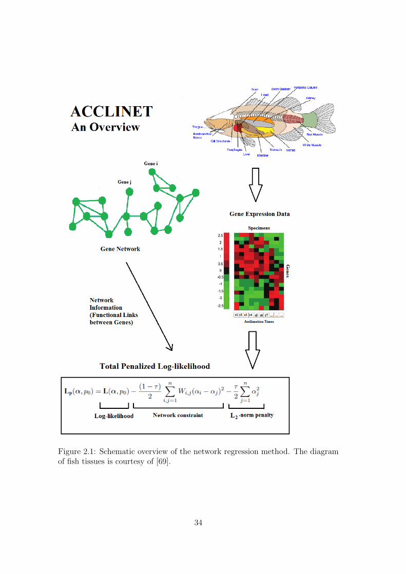
Figure 2.1: Schematic overview of the network regression method. The diagramof fish tissues is courtesy of [69].
34

be found in the NCBI Sequence Read Archive (SRA) under accession numbers
SRP018876 and SRP019202. All specimens were exposed to a temperature of
4 degrees Celsius (well above their ambient temperature) but for different time
periods. Once the network constraints are taken into account, the regression
method yields the following top 10 signature genes for acclimation in each tissue,
shown in Figure 2.2 with the associated p-values.
To evaluate the performance of AccliNet, we compare with the results obtained by
Cox regression with Lasso (L1) and ridge (L2) penalties on the same dataset. In
each case, parameter tuning is done by five-fold cross validation on the dataset. In
particular, four fifths of the dataset are used to train the model, and the remaining
fifth is used to test the performance. We use the parameter µ = 1− τ , which is
increased gradually in value from 0 to 1 with increments of step size 0.02. For
each value of µ, the performance of the model is evaluated 5 times, ie. using a
different fifth of the data as the test set in each case, with the remaining data as
training set. The results are shown in Figure 2.3.
We observe that AccliNet detects more signature genes than L1 Cox and
L2 Cox at all cut-offs. Hence, the incorporation of gene network information
clearly improves the performance of the algorithm with respect to more traditional
regression methods. To further confirm the contribution of the network informa-
tion to the performance of AccliNet, we compare the results obtained using the
actual network constraints (the graph G and weight matrix W), with randomized
graphs obtained by shuffling the edges and randomly reassigning the weights.
The comparison is shown in Figure 2.4. The curve corresponding to running
AccliNet with randomized network constraints is the average of 30 runs (which is
why it is smoother than the curve above). We observe that AccliNet using the
real network constraints performs far better than with the randomized constraints
at all cut-offs, which again shows that the network information is decisive for
algorithm performance.
To validate the results of the signature genes detected by AccliNet, we per-
form a literature review of acclimation studies in this field to see which genes have
been verified by experiment to be differentially expressed in each tissue during
35

Figure 2.2: Top 10 signature genes relevant for acclimation in each tissue accordingto the network-based regression, and the associated p-values.
heat stress. Figure 2.5 shows the genes from Figure 2.2 with relevant references
for each gene and tissue.
36

Figure 2.3: Comparison between number of signature genes detected by AccliNet(in red), L1 Cox (magenta), and L2 Cox (blue) at different cut-offs.
2.3 The AccliNet Algorithm
The AccliNet algorithm has been implemented in MATLAB, and is available at
the following source code repository:
https://github.com/pablosg713/AccliNet
The total penalised log-likelihood in Equation 2.8 can be maximised by alternating
between maximisation with respect to α and with respect to p0(t) [65]. The full
algorithm is shown below:
1. Initialise α = 0.
2. Compute Λ = I−W.
3. Repeat until convergence:
i. Repeat Newton-Raphson iteration:
a) Compute first derivative
L’p(α, p0) =∂Lp(α, p0)
∂α(2.9)
37

Figure 2.4: Comparison between number of signature genes detected by AccliNetusing real network constraints (in red) and using randomized network constraints(green) at different cut-offs. The curve corresponding to running randomizednetwork constraints is the average of 30 runs.
b) Compute second derivative
L”p(α, p0) =∂2Lp(α, p0)
∂α∂α′(2.10)
c) Update
α = α− {L”p(α, p0)}−1L’p(α, p0) (2.11)
ii. Update the Breslow estimator [65]:
p0(t) = 1/∑
m∈R(ti)
exp(D ′mα) (2.12)
4. Return α.
The use of the Newton-Raphson method to update α requires the inversion
of the Hessian matrix, which can often be computationally costly. An alternative
solution is reducing the covariant space from n (the number of genes) to k (the
38
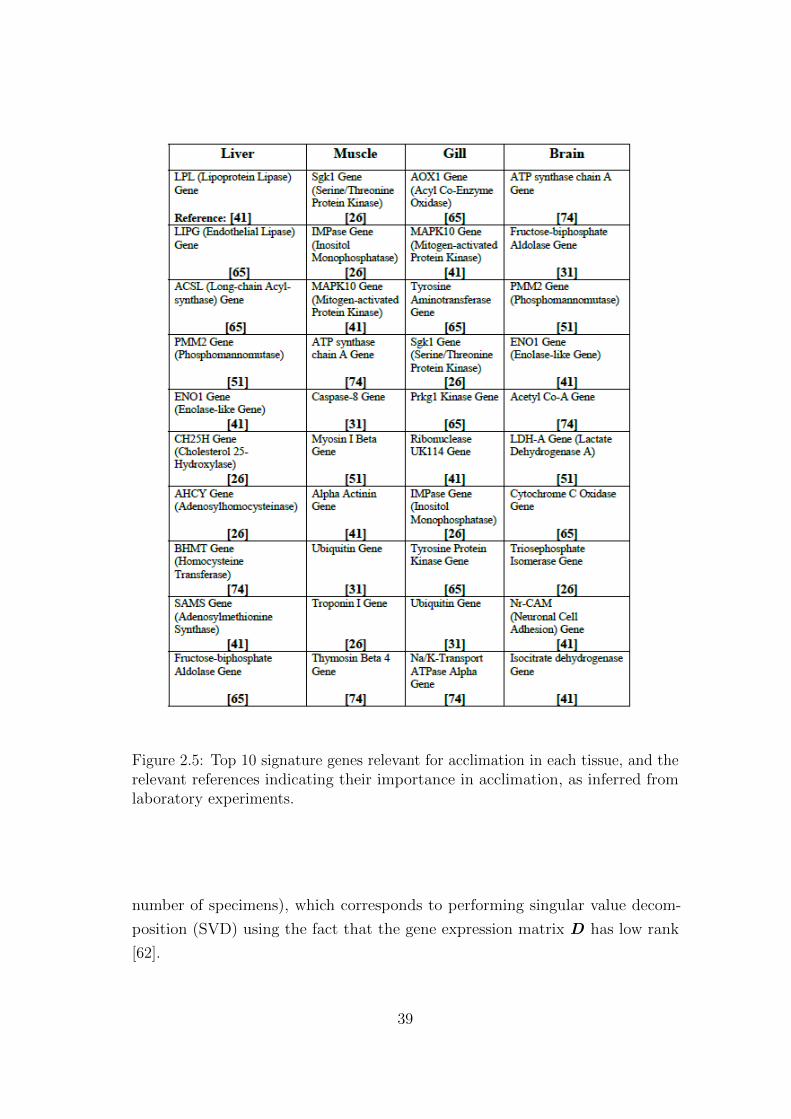
Figure 2.5: Top 10 signature genes relevant for acclimation in each tissue, and therelevant references indicating their importance in acclimation, as inferred fromlaboratory experiments.
number of specimens), which corresponds to performing singular value decom-
position (SVD) using the fact that the gene expression matrix D has low rank
[62].
39
2.4 Discussion of Results
We observe that the primary genes detected for skeletal muscle are the Sgk1
gene, IMPase gene, and MAPK10 gene, all important for signaling pathways and
involved in the inflammatory response to environmental stress [68]. As part of
this response, there is an inhibition of the JAK/STAT and growth factor signaling
pathway, to reduce cell proliferation and growth in adverse conditions (see Figure
2.6). This reduction in cell proliferation may represent an adaptive strategy for
the organism, to free energy resources normally used for cell growth so that they
can be used in the response to stress [69].
In particular, there is attentuation of the ERK group of MAP kinases, which
are phosphorylated in response to the binding of growth factor to cell-surface
receptors [73]. At the same time, cytokines activated by the NOD-like receptor
signaling pathway (NLR) converge on the MAPK pathway, and initiate apoptotic
signals in the damaged tissues. Also detected was a gene coding for caspase-8,
which is believed to mediate in initiation of apoptosis [71].
In the gill tissue, the MAPK10 and Sgk1 genes are also detected, which again
suggests an inflammatory response during acclimation to elevated temperatures.
In addition, we have AOX1, Prkg1 and the tyrosine aminotransferase gene, all of
which are involved in response to oxidative stress [50]. AOX1 increases β oxidation
of fatty acids and leads to production of peroxide, H2O2. During oxidative stress,
the cell uses NADPH to reduce glutathione and transform peroxide into H2O.
The β oxidation of fatty acids also serves as the main source of ATP production
for notothenioids under stressful conditions [50].
At the same time, tyrosine aminotransferase is up-regulated by changes in oxygen
tension [71]. The presence of reactive oxygen species may activate an inflammatory
response via the NLR signaling pathway, with activation of pro-inflammatory
cytokines and integration with downstream signaling in the MAPK pathway [73].
By contrast, the primary genes detected for the liver are lipase genes (LPL
and LIPG), which are involved in breakdown of lipids to make fatty acids available
to other tissues during acclimation [63]. Also present is the PMM2 gene, involved
40

in breakdown of simple sugars as a further energy source, and the ENO1 gene,
which is part of the glycolytic pathway, and thus suggests reduced oxygen during
some or all of the acclimation process [63].
In the brain, the genes detected are again involved in maintaining energy levels
during acclimation. Thus, we have the ATP synthase chain A gene, as well as a
fructose-biphosphate aldolase gene, PMM2, and acetyl co-A, which are involved
in metabolism of sugars for energy production under stressful conditions [73].
Figure 2.6: Schematic of the signaling cascade involved in the inflammatoryresponse to heat stress [71].
2.5 Conclusions
The use of network constraints allows us to incorporate prior knowledge about
functional links between genes into the AccliNet regression method, and thus
begin to uncover some of the signaling mechanisms involved in acclimation of
Antarctic organisms to changing conditions.
As shown in Section 2.3, AccliNet outperforms both L1 Cox and L2 Cox at
41

all cut-offs after all three methods have been trained on the same dataset by
five-fold cross-validation. To further confirm the importance of the network in-
formation to the performance of the algortihm, the AccliNet method using the
actual graph G and weight matrix W was compared with the use of randomized
graphs; again, the regression with the real network constraints detects far more
signature genes than using the randomized constraints.
The top signature genes detected by the AccliNet method suggest the following
adaptive strategy for Pagothenia borchgrevinki during acclimation to heat stress.
First, in skeletal muscle, there is an activation of signaling pathways that inhibit
cell growth and proliferation, in order to free energy resources so they can be used
in the stress response. The subsequent activation of pro-inflammatory cytokines
leads to an inflammation reaction on short timescales, with initiation of apoptosis
in damaged tissues [71].
Some inflammatory response is also detected in the gill tissue, coupled with
a reaction to oxidative stress due to the presence of reactive oxygen species. The
activation of signaling pathways involved in inflammation in skeletal muscle and
gills is followed by mobilization of energy stores in the liver. The action of lipases
breaks down lipids into fatty acids, which are then distributed to other tissues for
β oxidation, an important ATP source for notothenioids during acclimation to
heat stress [50].
The energy obtained from β oxidation is complemented by metabolism of simple
sugars in both the liver and other tissues such as the brain to maintain energy
levels. The detection of genes such as ENO1 also indicates activation of glycolytic
pathways, which suggests a reduction in oxygen supply during acclimation.
Reduced oxygen would agree with the findings of Thorne et al. (2010), which
suggest that hypoxia is a limiting factor for acclimation to elevated temperatures
for notothenioids on short timescales [50]. In addition, Huth and Place (2016)
found that gill tissue of Pagothenia borchgrevinki showed significant evidence of
oxidative stress during the acclimation process [74].
Although further studies are needed to identify other mechanisms of acclimation
42

in Antarctic organisms, the use of network-based regression holds considerable
promise in this field, as it allows us to incorporate knowledge of gene signaling
networks into the regression of gene expression data.
Broadly speaking, the general idea of network regression shares an aspect in
common with the “attention mechanism” in neural networks. In particular, the
regression considered here aims to determine which sets of genes are most im-
portant for acclimation in each tissue, while the attention mechanism seeks to
identify which parts of an input are most important to determining the output of
a neural network. Thus, in a general sense, both methods aim to isolate the part
of the input that is most relevant to producing a given ouput.
However, the implementation of the two methods is completely different, as
AccliNet follows the approach described earlier in this chapter, while the attention
mechanism typically uses a so-called “attention module”, with a system of soft
weights that are modified dynamically during runtime to focus attention first on
certain parts of the input and then on others [75].
Although AccliNet also uses weights to account for the strength of the link
between genes, these weights are based on a priori knowledge, and remain fixed
during runtime, and are not modified dynamically as in the case of the attention
mechanism. Further work on AccliNet could be directed at expanding the scale of
the gene networks considered in the regression, and the use of larger datasets to
draw more definitive conclusions about acclimation in different tissues.
43

44

Chapter 3
Modeling Distributions in
Metabolism using Autoencoders
3.1 Constructing the Model
In this chapter, we present a novel approach to modeling distributions in metabolism
using autoencoders. We start by modeling each metabolic pathway we are inter-
ested in as a directed graph, where the nodes are the compounds (or metabolites)
involved in the pathway. There is a directed edge from node A to node B if and
only if there is a reaction taking compound A as the reactant (or as one of the
reactants) and producing compound B as a product.
Note that multiple directed edges may converge on a single node, in the case of
multiple reactants combining to produce a single product compound. Conversely,
a single reactant may be broken up to give multiple products, so there may be
edges diverging from a single node towards multiple product nodes.
Typically, each reaction represented by an edge will be governed by a partic-
ular enzyme, which acts as a catalyst in that reaction. The rate at which the
reaction occurs will depend significantly on the concentrations of that enzyme,
but also on other factors such as temperature [5]. Our goal in metabolic modeling
is to estimate the reaction rates on each edge along the pathway, and thus track
the flow through the network of metabolic compounds. We are also interested in
how reaction rates vary with temperature, and potentially other factors as well
45
(they can be added later to our framework).
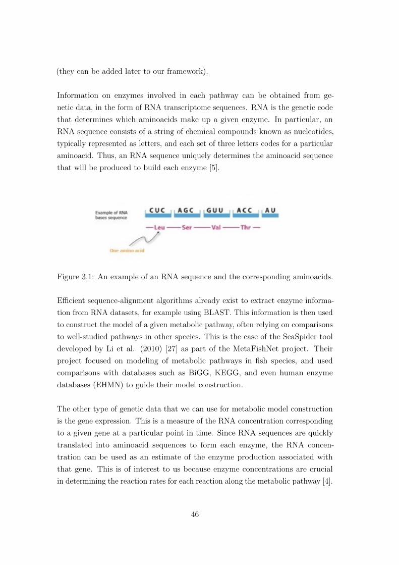
Information on enzymes involved in each pathway can be obtained from ge-
netic data, in the form of RNA transcriptome sequences. RNA is the genetic code
that determines which aminoacids make up a given enzyme. In particular, an
RNA sequence consists of a string of chemical compounds known as nucleotides,
typically represented as letters, and each set of three letters codes for a particular
aminoacid. Thus, an RNA sequence uniquely determines the aminoacid sequence
that will be produced to build each enzyme [5].
Figure 3.1: An example of an RNA sequence and the corresponding aminoacids.
Efficient sequence-alignment algorithms already exist to extract enzyme informa-
tion from RNA datasets, for example using BLAST. This information is then used
to construct the model of a given metabolic pathway, often relying on comparisons
to well-studied pathways in other species. This is the case of the SeaSpider tool
developed by Li et al. (2010) [27] as part of the MetaFishNet project. Their
project focused on modeling of metabolic pathways in fish species, and used
comparisons with databases such as BiGG, KEGG, and even human enzyme
databases (EHMN) to guide their model construction.
The other type of genetic data that we can use for metabolic model construction
is the gene expression. This is a measure of the RNA concentration corresponding
to a given gene at a particular point in time. Since RNA sequences are quickly
translated into aminoacid sequences to form each enzyme, the RNA concen-
tration can be used as an estimate of the enzyme production associated with
that gene. This is of interest to us because enzyme concentrations are crucial
in determining the reaction rates for each reaction along the metabolic pathway [4].
46

Our basic approach to metabolic modeling is the following. First, we extract the
enzyme information from RNA transcriptome data and use that to construct the
directed graph representing the metabolic pathway. Next, for each edge along the
pathway, we wish to model the unknown data-generating distribution P (X) that
generates the gene expression values for that enzyme, given only samples drawn
from X.
Although the unknown distribution could potentially be quite complicated, with
multiple modes, we can use recent results for autoencoders to tackle this problem.
In particular, as shown in Bengio et al. (2013) [2], if we construct a Markov chain
that alternately adds noise to the data, and learns to reconstruct the original
input from the noisy version using denoising autoencoders, then the stationary
distribution of the Markov chain will always converge to the true, unknown distri-
bution P (X).
More formally, we can take each sample X and map it to X ′ by adding noise from
some known corruption distribution Pc(X′ | X). We then use as training data
the set of pairs (X,X ′), where X ∼ P (X) and X ′ ∼ Pc(X′ | X), and train an
autoencoder to recover X from X ′, through the learned distribution Pθ(X,X′).
The training criterion is to minimise
L(θ) = −E[logPθ(X,X′)], (3.1)
with the expectation being over the joint distribution
P (X,X ′) = P (X)Pc(X′ | X). (3.2)
We can define the following Markov chain:
Xt ∼ Pθ(X | X ′t−1)
X ′t ∼ Pc(X′ | Xt) (3.3)
47
As proven in Bengio et al. (2013) [2], the stationary distribution of this Markov
chain converges to P (X).
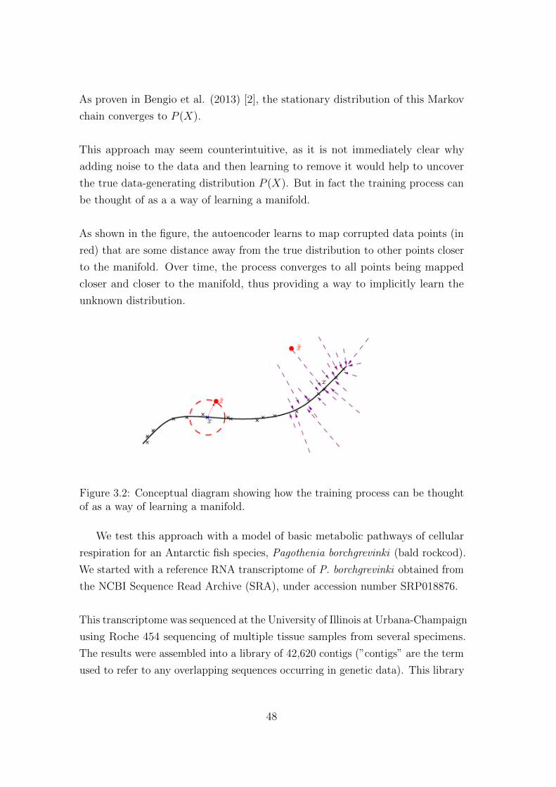
This approach may seem counterintuitive, as it is not immediately clear why
adding noise to the data and then learning to remove it would help to uncover
the true data-generating distribution P (X). But in fact the training process can
be thought of as a a way of learning a manifold.
As shown in the figure, the autoencoder learns to map corrupted data points (in
red) that are some distance away from the true distribution to other points closer
to the manifold. Over time, the process converges to all points being mapped
closer and closer to the manifold, thus providing a way to implicitly learn the
unknown distribution.
Figure 3.2: Conceptual diagram showing how the training process can be thoughtof as a way of learning a manifold.
We test this approach with a model of basic metabolic pathways of cellular
respiration for an Antarctic fish species, Pagothenia borchgrevinki (bald rockcod).
We started with a reference RNA transcriptome of P. borchgrevinki obtained from
the NCBI Sequence Read Archive (SRA), under accession number SRP018876.
This transcriptome was sequenced at the University of Illinois at Urbana-Champaign
using Roche 454 sequencing of multiple tissue samples from several specimens.
The results were assembled into a library of 42,620 contigs (”contigs” are the term
used to refer to any overlapping sequences occurring in genetic data). This library
48
was annotated by using BLASTx and looking for matches in the SwissProt and
UniProt/TrEMBL databases to create the reference transcriptome [11].
We then used the SeaSpider tool to map sequences in the reference transcriptome
to MetaFishNet genes and thus construct the directed graph corresponding to each
metabolic pathway. As mentioned previously, we focused only on those pathways
involved in respiration so that the size of the model would be more tractable
to analysis. We also broke up the larger graph into four parts or subgraphs for
greater ease during training.
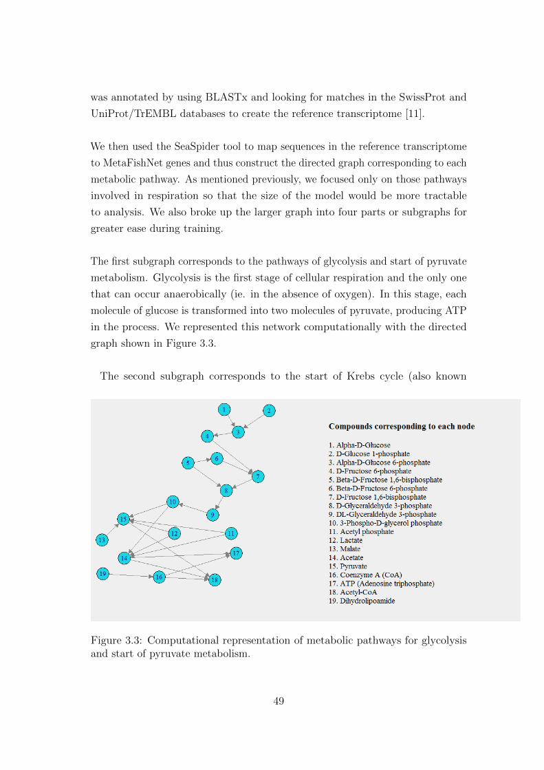
The first subgraph corresponds to the pathways of glycolysis and start of pyruvate
metabolism. Glycolysis is the first stage of cellular respiration and the only one
that can occur anaerobically (ie. in the absence of oxygen). In this stage, each
molecule of glucose is transformed into two molecules of pyruvate, producing ATP
in the process. We represented this network computationally with the directed
graph shown in Figure 3.3.
The second subgraph corresponds to the start of Krebs cycle (also known
Figure 3.3: Computational representation of metabolic pathways for glycolysisand start of pyruvate metabolism.
49

as the Citric Acid Cycle). In this stage of respiration, the molecule acetyl-CoA is
combined with oxaloacetate to yield citrate, and coenzyme A is released in the pro-
cess. We represented this network computationally with the graph shown in Figure
3.4. Note that some of the nodes and edges have been rearranged for compactness.
Figure 3.4: Computational representation corresponding to the start of Krebscycle, also known as the Citric Acid Cycle.
The third subgraph corresponds to the continuation of Krebs cycle and start
of glutamate metabolism. Finally, we have the last subgraph of the model, which
is the metabolic pathway corresponding to the electron transport chain. In this
stage, ATP is produced in the presence of oxygen; oxygen molecules then take
up electrons to form O2−, and protons to form H2O. As mentioned previously,
each reaction represented by an edge will be governed by a particular enzyme,
which acts as a catalyst in that reaction. For each edge along the pathway,
we wish to model the unknown data-generating distribution P (X) that gener-
ates the gene expression values for that enzyme, given only samples drawn from X.
We train the autoencoder using gene expression data for Pagothenia borchgrevinki
found in the NCBI Sequence Read Archive (SRA) under accession numbers
SRP018876 and SRP019202. The data is corrupted by using simple Gaussian
noise as the corruption distribution Pc(X′ | X). Thus, the autoencoder is trained
50

Figure 3.5: Computational representationcorresponding to the continuation ofKrebs cycle and start of glutamate metabolism.
Figure 3.6: Computational representation for the electron transport chain.
with the set of pairs (X,X ′), where X ∼ P (X) and X ′ ∼ Pc(X′ | X), and learns
to recover X from X ′, through the learned distribution Pθ(X,X′).
The structure of the autoencoder is shown in Figure 3.7. The encoder part
consists of two hidden layers. The first layer has 32 fully connected nodes, and
uses batch normalisation, and activation with rectified linear units (ReLU). The
second layer has 128 fully connected nodes, and also uses rectified linear units for
activation.
51
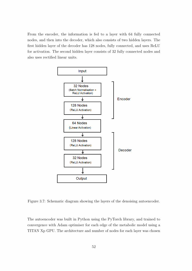
From the encoder, the information is fed to a layer with 64 fully connected
nodes, and then into the decoder, which also consists of two hidden layers. The
first hidden layer of the decoder has 128 nodes, fully connected, and uses ReLU
for activation. The second hidden layer consists of 32 fully connected nodes and
also uses rectified linear units.
Figure 3.7: Schematic diagram showing the layers of the denoising autoencoder.
The autoencoder was built in Python using the PyTorch library, and trained to
convergence with Adam optimiser for each edge of the metabolic model using a
TITAN Xp GPU. The architecture and number of nodes for each layer was chosen
52

based on the best performance after trying a wide range of possible architectures.
The source code used for this chapter of the thesis is available at the follow-
ing repository: https://github.com/pablosg713/Autoencoder
3.2 Evaluating Performance of Autoencoder Ap-
proach
Once training is complete, we obtain a distribution of reaction rates for each edge
of the directed graph. We can now use this to model the response of metabolic
pathways under different conditions. We initially run the model at ambient tem-
perature (unstressed conditions) for P. borchgrevinki.
We assume an average rate of glucose consumption of 6 µmol min−1g−1, and
then calculate the flux of metabolites through each edge of the directed graph by
sampling from the distribution governing reaction rates on that edge. Sampling
is repeated 10 times and averaged for each edge to remove influence of outlying
values on the reaction rate.
The results of the initial model run at ambient temperature show some interest-
ing features (see Figure 3.6). In particular, the model yields a level of acetate
production of 0.043 µmol, that is, practically negligible. Similarly, for pyruvate,
the level of production reported by the model is just 0.051 µmol, again negli-
gible for practical purposes. Since acetate and pyruvate are byproducts that
can be damaging to the organism if accumulated in high levels, the fact that
their values are minimal is an indication of normal, healthy respiration at this stage.
At the same time, ATP production in the model is 0.961 µmol, very close to 1
µmol, a reasonable value for this stage of respiration under ambient conditions.
ATP stands for adenosine triphosphate and is the molecule used to store energy in
each cell. Sufficient ATP production is once more an indication that this metabolic
pathway is working normally under these conditions.
Next, we raise the temperature in the model to 4 degrees Celsius, well above the
53

ambient temperature for P. borchgrevinki (heat-stressed conditions). We update
the distributions of reaction rates for each edge and run the model under the new
scenario. The results of the model are quite different in this case.
We soon see an accummulation of both acetate (at 0.822 µmol min−1g−1) and
pyruvate (at 1.034 µmol min−1g−1), as the organism’s metabolism is unable to
rid itself of these byproducts at the normal rate. At the same time, ATP produc-
tion drops to 0.455 µmol min−1g−1, less than half its original value at ambient
temperature. Altogether, these features indicate a significant disruption in this
metabolic pathway under heat-stressed conditions.
To evaluate the performance of this approach, we will compare to the afore-
mentioned MetaFishNet model, and to a traditional Bayesian inference model.
3.2.1 Traditional Bayesian Inference Model
The Bayesian inference model we will use for comparison is constructed as follows.
We use the same directed graph as before.
Then, for each edge along the pathway, we use a Gaussian prior, with mean
µ and standard deviation σ, which will serve as a prior distribution before learning
from any of the gene expression data. Finally, we use gene expression data taken
from multiple specimens and different temperatures to update the parameters of
the distribution for each edge, and thus ”train” the model to have a more accurate
distribution of reaction rates for each part of the pathway.
More formally, suppose a is a parameter governing the distribution of the reaction
rate r, so that
r ∼ p(r | a). (3.4)
Let q1, ..., qn be a set of n observations of the reaction rate obtained from gene
expression data. We use the Bayesian approach and treat the temperature T as a
hyperparameter. Then the parameter update is done using
p(a | q1, ..., qn, T ) =p(q1, ..., qn | a)p(a | T )
p(q1, ..., qn | T )(3.5)
54
The prediction for a reaction rate given the data already seen and a temperature
is done using the posterior predictive distribution,
p(r | q1, ..., qn, T ) =
∫a
p(r | a)p(a | q1, ..., qn, T )da. (3.6)
The same approach could be applied for a prior having multiple parameters, so
a vector ~a instead of a, and multiple hyperparameters, if we considered factors
other than temperature that could influence reaction rates.
As mentioned previously, we initially use a Gaussian prior with mean µ and
standard deviation σ (the values of µ and σ differ for each enzyme and are up-
dated with new data as it is received). Recall that the Gaussian (or Normal)
distribution is given by the probability density function
p(x | µ, σ2) =1√
2πσ2e
−(x−µ)2
2σ2 , (3.7)
where µ is the mean and σ2 is the variance of the distribution.
3.2.2 Updating Distribution Parameters
The parameter update for this distribution given new data y1, ..., yn is done using
Bayes’ theorem:
p(µ | y1, ..., yn) =p(y1, ..., yn | µ)p(µ)∫p(y1, ..., yn | µ′)p(µ′)dµ′
, (3.8)
where p(y1, ..., yn | µ) is the likelihood and p(µ) is the prior distribution. In the
case of the Normal distribution, this computation is simplified by using a conjugate
prior. In particular, with a prior of the form N(µ0, σ20), the parameter update can
be calculated with the closed form expression
µ∗ =µ0τ0 + τ
∑yi
nτ + τ0, (3.9)
55

where µ∗ is the new mean, τ is the precision equal to 1σ2 , and τ0 is equal to 1
σ20. At
the same time, the new variance σ2∗ is given by the expression
1
σ2∗
= nτ + τ0. (3.10)
The following is an example in R showing how to update µ given 10 new data
points.
Figure 3.8: Bayesian parameter update for µ given 10 new data points.
To reflect the dependence on temperature, T is treated as a hyperparameter that
affects the value of µ0. In particular, µ0 is sampled from a Gamma distribution
with parameters T and β. In turn, this distribution is also updated dynamically
based on new data. For each new data point received, T is assumed to be known
(ie. we know at what temperature the data has been collected), so it is the
parameter β that is the object of the Bayesian inference. The update is again
done using Bayes’ theorem:
p(β | x1, ..., xn) =p(x1, ..., xn | β)p(β)∫p(x1, ..., xn | β′)p(β′)dβ′
, (3.11)
where x1, ..., xn are the new data points, p(x1, ..., xn | β) is the likelihood and p(β)
is the prior distribution.
The use of conjugacy can simplify the computation in this case as well. In
56
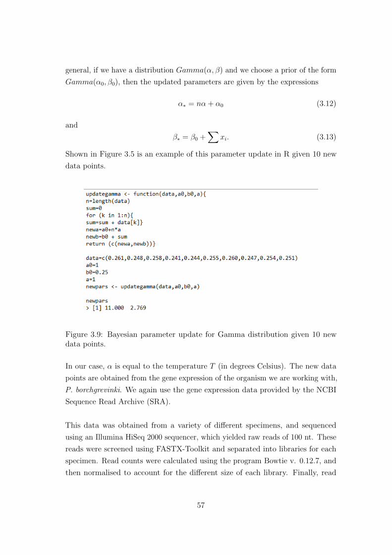
general, if we have a distribution Gamma(α, β) and we choose a prior of the form
Gamma(α0, β0), then the updated parameters are given by the expressions
α∗ = nα + α0 (3.12)
and
β∗ = β0 +∑
xi. (3.13)
Shown in Figure 3.5 is an example of this parameter update in R given 10 new
data points.
Figure 3.9: Bayesian parameter update for Gamma distribution given 10 newdata points.
In our case, α is equal to the temperature T (in degrees Celsius). The new data
points are obtained from the gene expression of the organism we are working with,
P. borchgrevinki. We again use the gene expression data provided by the NCBI
Sequence Read Archive (SRA).
This data was obtained from a variety of different specimens, and sequenced
using an Illumina HiSeq 2000 sequencer, which yielded raw reads of 100 nt. These
reads were screened using FASTX-Toolkit and separated into libraries for each
specimen. Read counts were calculated using the program Bowtie v. 0.12.7, and
then normalised to account for the different size of each library. Finally, read
57
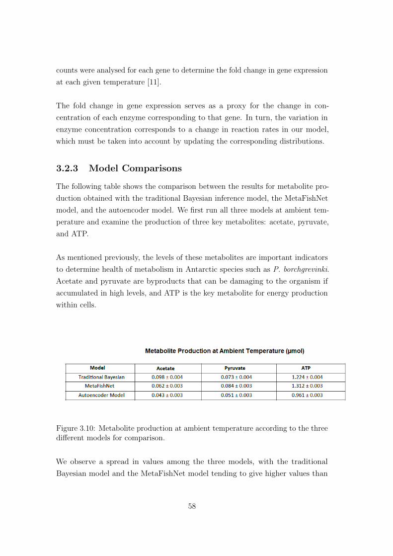
counts were analysed for each gene to determine the fold change in gene expression
at each given temperature [11].
The fold change in gene expression serves as a proxy for the change in con-
centration of each enzyme corresponding to that gene. In turn, the variation in
enzyme concentration corresponds to a change in reaction rates in our model,
which must be taken into account by updating the corresponding distributions.
3.2.3 Model Comparisons
The following table shows the comparison between the results for metabolite pro-
duction obtained with the traditional Bayesian inference model, the MetaFishNet
model, and the autoencoder model. We first run all three models at ambient tem-
perature and examine the production of three key metabolites: acetate, pyruvate,
and ATP.
As mentioned previously, the levels of these metabolites are important indicators
to determine health of metabolism in Antarctic species such as P. borchgrevinki.
Acetate and pyruvate are byproducts that can be damaging to the organism if
accumulated in high levels, and ATP is the key metabolite for energy production
within cells.
Figure 3.10: Metabolite production at ambient temperature according to the threedifferent models for comparison.
We observe a spread in values among the three models, with the traditional
Bayesian model and the MetaFishNet model tending to give higher values than
58

the autoencoder model. However, among the three models, the autoencoder model
is closest to the values found in the literature [45,41]. We next consider the case
of metabolic response under heat stress. We run the three models in the scenario
of higher temperature (4 degrees Celsius) and compare the metabolite production
predicted by each model.
Figure 3.11: Metabolite production under heat stress according to the threedifferent models for comparison.
The results are shown in Figure 3.11. All three models predict a significant increase
in acetate and pyruvate compared to ambient temperature, and a sharp decrease
in ATP production, but again the third model is closer to literature values [45,41].
Thus, there is an advantage in using the approach with denoising autoencoders as
compared to more traditional approaches.
Next we will test the robustness to noise of the autoencoder model compared to a
traditional Bayesian inference model.
3.2.4 Robustness to Noise
To test robustness, we first run each model on normal (uncorrupted) data, and
then progressively add Gaussian noise to see how this affects performance. In
particular, the noise is drawn from the distribution N(0, 0.5), and the data to be
corrupted is chosen at random from the entire dataset. The performance of each
model, as more noise is added, is compared to the performance with the original,
uncorrupted data, which acts as a baseline for comparison.
The results are shown in the following figure, with the Bayesian model shown
59

in green and the autoencoder model in blue. Performance level is given as a
percentage relative to the baseline.
Figure 3.12: Robustness to noise of the Bayesian model (in green) and theautoencoder model (in blue).
Initially, the performance of both models is unaffected when the amount of noise
is small (affecting less than 5 percent of the data). However, once more than 5
percent of the data has been corrupted, the performance of the Bayesian model
declines rapidly, while the autoencoder model continues to perform well even at
15 percent.
Thus, the autoencoder model is much more robust to noise than the Bayesian
model, which is an important advantage in many situations where the data has
been corrupted during the process of collection or from other sources. Note
that here we have considered normally-distributed (Gaussian) noise, as this is
most common in real-world applications. However, a possible direction for future
research would be to examine the robustness of these models to other types of
noise (with different distributions, such as Poisson, Gamma, etc.) and evaluate
their performance in that case.
In the following chapter, we will consider modeling the metabolic response with a
different type of neural network, a generative adversarial network, and we will
60

compare it to the autoencoder model as well as to the other models to see if
performance can be improved.
61

62
Chapter 4
A Novel Approach using GANs
4.1 Constructing the Model
In this chapter, we present a different approach to modeling the changes in enzyme
concentrations over time during temperature increases. We treat the data as a
time series, and use a Generative Adversarial Network (GAN) to learn an SDE
path through the data points. In particular, the GAN learns to predict the next
value St+δt | St from St and δt.
Generative Adversarial Networks (GANs) are able to learn through a competitive
process involving two players, one referred to as the generator and the other as
the critic or discriminator. The generator attempts to produce synthetic samples
imitating the true distribution, and the critic tries to discern whether the sample
produced is real or synthetic. The competition between the two players drives the
process and improves the performance of the GAN over time.
The goal is to obtain better predictions of how reaction rates vary on each edge
of our directed graph from Chapter 3. Thus, we use the same simplified graph
of the metabolic pathways of cellular respiration for the Antarctic fish species,
Pagothenia borchgrevinki (bald rockcod). The larger graph is again divided into
four subgraphs for greater ease during training.
The subgraphs are shown here again for completeness, before diving into the
details of the GAN that will be used to predict reaction rates on each edge. The
63
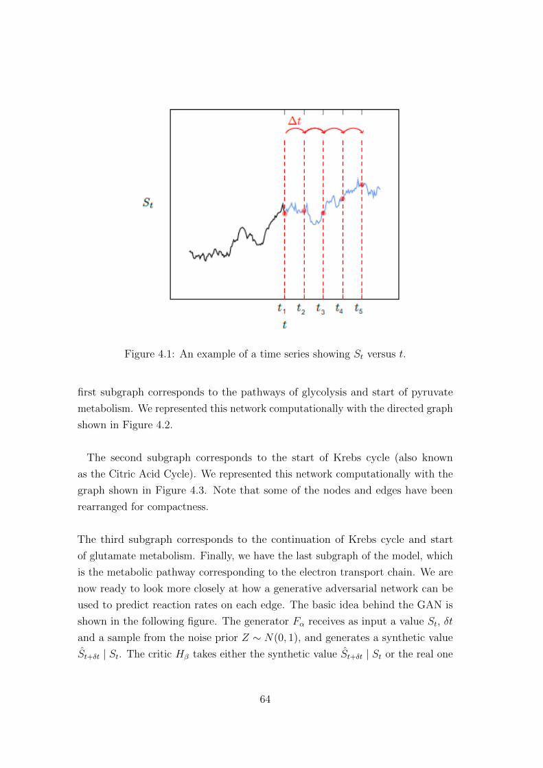
Figure 4.1: An example of a time series showing St versus t.
first subgraph corresponds to the pathways of glycolysis and start of pyruvate
metabolism. We represented this network computationally with the directed graph
shown in Figure 4.2.
The second subgraph corresponds to the start of Krebs cycle (also known
as the Citric Acid Cycle). We represented this network computationally with the
graph shown in Figure 4.3. Note that some of the nodes and edges have been
rearranged for compactness.
The third subgraph corresponds to the continuation of Krebs cycle and start
of glutamate metabolism. Finally, we have the last subgraph of the model, which
is the metabolic pathway corresponding to the electron transport chain. We are
now ready to look more closely at how a generative adversarial network can be
used to predict reaction rates on each edge. The basic idea behind the GAN is
shown in the following figure. The generator Fα receives as input a value St, δt
and a sample from the noise prior Z ∼ N(0, 1), and generates a synthetic value
St+δt | St. The critic Hβ takes either the synthetic value St+δt | St or the real one
64
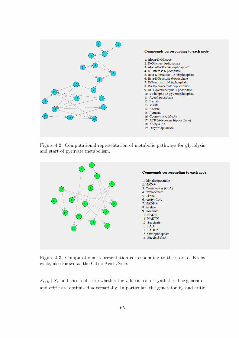
Figure 4.2: Computational representation of metabolic pathways for glycolysisand start of pyruvate metabolism.
Figure 4.3: Computational representation corresponding to the start of Krebscycle, also known as the Citric Acid Cycle.
St+δt | St, and tries to discern whether the value is real or synthetic. The generator
and critic are optimised adversarially. In particular, the generator Fα and critic
65

Figure 4.4: Computational representationcorresponding to the continuation ofKrebs cycle and start of glutamate metabolism.
Figure 4.5: Computational representation for the electron transport chain.
Hβ are trained to solve the following minimax game using the Wasserstein distance
[16]:
minα
maxβ
E[Hβ(St+δt | St, δt)− E[Hβ(St+δt | St, δt)]
]. (4.1)
To solve this minimax problem, we interleave gradient updates for Fα and Hβ
optimising the following problems [15]:
minα
−1
j
j∑k=1
Hβ(Sk+δt | Sk, δt) (4.2)
66
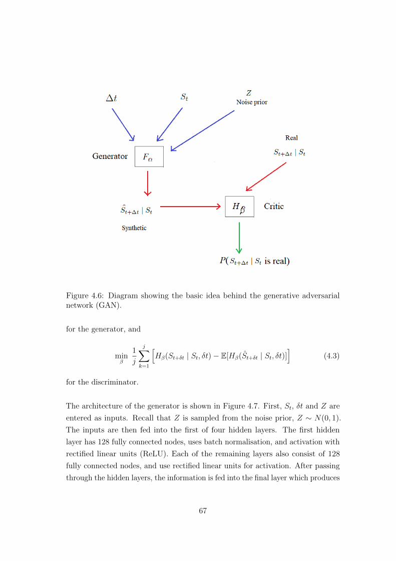
Figure 4.6: Diagram showing the basic idea behind the generative adversarialnetwork (GAN).
for the generator, and
minβ
1
j
j∑k=1
[Hβ(St+δt | St, δt)− E[Hβ(St+δt | St, δt)]
](4.3)
for the discriminator.
The architecture of the generator is shown in Figure 4.7. First, St, δt and Z are
entered as inputs. Recall that Z is sampled from the noise prior, Z ∼ N(0, 1).
The inputs are then fed into the first of four hidden layers. The first hidden
layer has 128 fully connected nodes, uses batch normalisation, and activation with
rectified linear units (ReLU). Each of the remaining layers also consist of 128
fully connected nodes, and use rectified linear units for activation. After passing
through the hidden layers, the information is fed into the final layer which produces
67

Figure 4.7: Schematic diagram showing the layers of the generator architecture.
the output St+δt | St. This output will then be passed to the discriminator.
The architecture of the discriminator mirrors that of the generator, except that it
receives only a single input in the first layer - either the synthetic value St+δt | Stproduced by the generator, or a real value St+δt | St. From the input layer, the
information is again fed into the first of four hidden layers.
68

The first hidden layer has 128 fully connected nodes, uses batch normalisation,
and activation with rectified linear units (ReLU). Each of the remaining hidden
layers also consist of 128 fully connected nodes, and use rectified linear units for
activation. Finally, the information passes to the last layer, which produces the
output, in this case the probability that the input was a real value instead of a
synthetic one produced by the generator.
Both generator and discriminator were built in Python using the PyTorch li-
brary, and trained to convergence with Adam optimiser for each edge of the
metabolic model using a TITAN Xp GPU. The architecture and number of nodes
for each layer was chosen based on the best performance after trying a wide range
of possible architectures.
The source code used for this chapter of the thesis is available at the follow-
ing repository: https://github.com/pablosg713/GAN
4.2 Evaluating Performance of GAN Model
4.2.1 Model Comparisons
To evaluate the performance of this approach, we will compare to a traditional
Bayesian inference model, the MetaFishNet model, and to the autoencoder model
from the previous chapter. As in Chapter 3, we first run all three models at ambi-
ent temperature and examine the production of three key metabolites: acetate,
pyruvate, and ATP.
As mentioned previously, the levels of these metabolites are important indicators
to determine health of metabolism in Antarctic species such as P. borchgrevinki.
Acetate and pyruvate are byproducts that can be damaging to the organism if
accumulated in high levels, and ATP is the key metabolite for energy production
within cells.
Figure 4.9 shows the comparison between the results for metabolite production
obtained with all four models. We observe a range of values among these models,
69

Figure 4.8: Schematic diagram showing the layers of the discriminator architecture.
with the traditional Bayesian model and the MetaFishNet model tending to give
higher values than the autoencoder and GAN models. However, the metabolite
production predicted by the GAN model is relatively close to the autoencoder
model.
We next consider the case of metabolic response under heat stress. We run
70
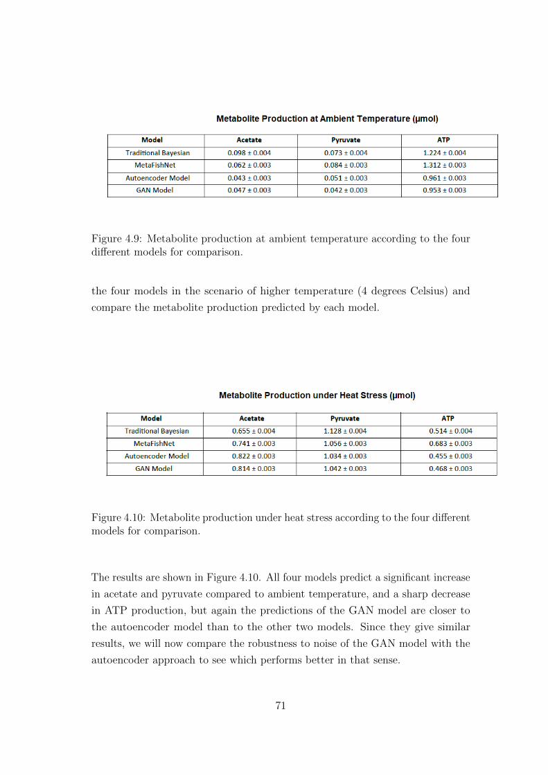
Figure 4.9: Metabolite production at ambient temperature according to the fourdifferent models for comparison.
the four models in the scenario of higher temperature (4 degrees Celsius) and
compare the metabolite production predicted by each model.
Figure 4.10: Metabolite production under heat stress according to the four differentmodels for comparison.
The results are shown in Figure 4.10. All four models predict a significant increase
in acetate and pyruvate compared to ambient temperature, and a sharp decrease
in ATP production, but again the predictions of the GAN model are closer to
the autoencoder model than to the other two models. Since they give similar
results, we will now compare the robustness to noise of the GAN model with the
autoencoder approach to see which performs better in that sense.
71

4.2.2 Robustness to Noise
To test robustness, we first run each model on normal (uncorrupted) data, and
then progressively add Gaussian noise to see how this affects performance. In
particular, the noise is drawn from the distribution N(0, 0.5), and the data to be
corrupted is chosen at random from the entire dataset. The performance of each
model, as more noise is added, is compared to the performance with the original,
uncorrupted data, which acts as a baseline for comparison.
The results are shown in the following figure, with the GAN model shown in red
and the autoencoder model in blue.
Figure 4.11: Robustness to noise of the GAN model (in red) and the autoencodermodel (in blue).
Initially, the performance of both models is unaffected when the amount of noise
is small (affecting less than 10 percent of the data). However, once more than
10 percent of the data has been corrupted, the performance of the GAN model
declines rapidly, while the autoencoder model continues to perform well even at
15 percent.
Thus, the GAN model is less robust to noise than the autoencoder model, which
can be a disadvantage in some situations, even if the accuracy of the two models
is similar when there is little or no noise. Note that here we have considered
72

normally-distributed (Gaussian) noise, as this is most common in real-world appli-
cations; however, a possible direction for future research would be to examine the
robustness of these models to other types of noise (with different distributions,
such as Poisson, Gamma, etc.) and evaluate their performance in that case.
73

74

Chapter 5
The PhylSim Package
In this chapter, we shift our focus from short-term metabolic responses to long-
term evolution and adaptation to changing conditions. In particular, we introduce
the PhylSim package, which simulates the evolution of traits on a phylogeny,
allowing the user to freely vary speciation rates and evolutionary models over the
course of the simulation.
PhylSim makes use of the ‘pcmabc’ and ‘yuima’ packages in R, so it can interpret
any of the SDE models accepted by ‘yuima’, ie. single and multivariable diffusion
processes, Brownian motion, Ornstein-Uhlenbeck with and without jumps, etc.
The user only needs to specify which model to use for each regime, and the times
at which the regimes change. The regimes for the evolutionary models need not
match the regimes for the speciation rates, in order to give the user more flexibility.
At the branch level, PhylSim uses the function ‘simulate sde on branch’ from
‘pcmabc’ package to simulate trait evolution on branch segments. The length of
these segments can be specified by the user. In each segment, the trait evolves
according to the evolutionary model corresponding to that time period (depending
on the regime that segment is in). Also, the probability of branching occurring in
a given segment depends on the speciation regime for that segment. Thus, the
speciation rate is time dependent, and also trait dependent, as the user can set
the rates to change in a given regime when the value of the trait exceeds a certain
threshold.
75

Figure 5.1: Diagram showing the basics of the PhylSim package.
The schematic diagram in Figure 5.1 summarises the basics of how PhylSim
works. Also, an example of the early stages of a simulation with an arbitrary
numerical trait is shown in Figures 5.2 - 5.4. In Figure 5.4, the speciation rate
is set to increase after t = 10, which results in increased branching after that time.
The main function in the PhylSim package is called as follows:
run1← phylsim(time, X0, step, duration, modeltimes, modeldefs, spec-
times, specprob1, specprob2, traitval, maxtime, filename)
Here, ‘time’ is the starting time of the simulation, and ‘X0’ is the initial value (in
the single variable case; it can also be a vector of trait values for the multivari-
76

Figure 5.2: Simulation until t = 4, with trait value following an Ornstein-Uhlenbeckprocess with jumps.
Figure 5.3: Simulation until t = 10, with trait value following an Ornstein-Uhlenbeck process with jumps.
Figure 5.4: Simulation until t = 15, with increased speciation rate after t = 10.
able case). The argument ‘step’ is the step size for SDE solving throughout the
simulation.
77
Next, ‘modeltimes’ is a vector of times indicating when to change the evolu-
tionary model of the simulation (regime changes); this vector can be of any length
specified by the user, provided it is of the same length as ‘modeldefs’. The argu-
ment ‘modeldefs’ indicates which evolutionary model to use for each regime (the
model names are passed as strings). Each model name must be defined previously,
in the same way as in the ‘yuima’ package. A typical model definition would be
yuima.a←yuima::setModel (drift=”-(x-1)”, diffusion=”0.1”,
jump.coeff=”0.1”, measure=list(intensity=”1”, df=list(”dnorm(z,0,1)”)),
measure.type=”CP”, state.variable=”x”, solve.variable=”x”)
for a model with drift, diffusion and random jumps in the value of the trait.
Next, the argument ‘spectimes’ is a vector of times indicating when to change
the speciation rate regime. The argument ‘traitval’ is a vector of threshold trait
values; if a trait exceeds the threshold value in its regime, the speciation rate is set
to the value given by ‘specprob2’, otherwise the default is given by ‘specprob1’.
PhylSim follows Cox’s method from the ‘pcmabc’ package, and relies on the
‘yuima’ package for robust solution of stochastic differential equations on each
branch of the phylogeny. The PhylSim package was developed in R, and the
source code is available at the following repository:
https://github.com/pablosg713/PhylSim
A recent publication regarding PhylSim can be found here:
https://www.biorxiv.org/content/10.1101/2020.05.13.094706v1
5.1 Simulation of An Adaptive Radiation
As an example, we consider the adaptive radiation of Antarctic notothenioids in
the last 35 million years, during the period of cooling of the Southern Ocean. The
trait value we consider is the number of copies of a protein kinase gene, Prkg1-201,
which is found in all Antarctic notothenioids and their temperate relatives. Since
Prkg1-201 is a key mediator in the nitric oxide cycle, this gene is believed to have
been preferentially duplicated in Antarctic notothenioids in reponse to oxidative
78

stress as the climate cooled [26]. The number of copies in each species is the value
to which the Ornstein-Uhlenbeck process tends over time.
The Antarctic species we consider are: Parachaenichthys charcoti (Antarctic
dragonfish) [30]; Dissostichus mawsoni (Antarctic toothfish) [31]; Notothenia
coriiceps (Antarctic bullhead notothen) [32]; Chaenocephalus aceratus (blackfin
icefish) [33]; Chionodraco myersi (Myer’s icefish) [34]; Pseudochaenichthys geor-
gianus (South Georgia icefish) [35]; and Harpagifer antarcticus (Antarctic spiny
plunderfish) [35].
The temperate species are: Eleginops maclovinus (Patagonian robalo) [31]; Bovich-
tus variegatus (New Zealand thornfish) [36]; Bovichtus diacanthus (Tristan klipfish)
[37]. These species were chosen based on the availability of genetic sequence data,
and to be broadly representative of the main lineages of Antarctic and temperate
notothenioids.
We simulate the change in the environmental conditions in this case by setting
three different regimes. The first regime, from t = 0 to t = 12 Myrs, corresponds to
a period of relatively stable temperatures in the Southern Ocean around 8 degrees
Celsius, as described by Crame (2018) [38]. During this period, the simulation
follows an Ornstein-Uhlenbeck process with a moderate speciation rate due to the
climate conditions.
The second regime is a period of warming of the Southern Ocean, between
t = 12 and t = 18 Myrs, in which the temperature increases to about 12 degrees
[38]. During this time, the speciation rate is significantly reduced, and there are
smaller jumps in the value of the trait in the Ornstein-Uhlenbeck process.
The third regime, from t = 18 to t = 35 Myrs (ie. the present day, since
the simulation starts at 35 million years ago), corresponds to the cooling of the
Southern Ocean to current temperatures, with increased glacial cycles in the last
5 million years [38]. During this time, the speciation rate increases significantly,
not only as a result of the change in temperature, but also due to repeated frag-
mentation of breeding populations caused by advance and retreat of the glaciers
(the so-called biodiversity pump) [29].
79

The results of the simulation are shown in Figure 5.5. We observe that the
increased rate of speciation in the last 5-10 million years is clearly reflected in the
simulation, with a notable increase in the rate of branching during that regime.
Note that extinct lineages are also shown in the simulation for completeness.
Antarctic species are labeled in black, related temperate species are labeled in red.
Time is in millions of years.
These results agree with the findings of Near at al. (2012) [39], which sug-
gest that although antifreeze proteins evolved in Antarctic fish more than 20
million years ago, the main diversification of species occurred only in the last 5-10
million years of their evolution. From the simulated phylogeny, we can also obtain
Figure 5.5: Simulated phylogeny of Antarctic notothenioids for the last 35 millionyears, showing adaptive radiation during period of cooling of the Southern Ocean.
a plot of the effective population size of notothenioids over time. The results are
shown in Figure 5.6. The effective population size (y-axis) is given as a relative
measure, not in number of individuals. Time (x-axis) is given in millions of years
ago. Note the population bottlenecks which appear in the last 5 million years, as
a result of increased glacial cycles during this time.
80

Figure 5.6: Variation in effective population size of Antarctic notothenioids overthe last 35 Myrs.
5.2 Multivariate Simulation
The PhylSim package can also handle simulations with multiple trait values
evolving together in time. Hence, the above simulation could be run considering
multiple kinase genes, or even entire gene families, to test for other hypotheses
of evolution and adaptation. It is enough to define ‘X0’ to be a vector of trait
values of interest, and to specify the evolutionary model to be a multivariate
Ornstein-Uhlenbeck process, rather than single variable.
As an example, we consider the Antarctic species from the previous section,
and simulate their diversification in the last 10 million years. The trait values
we consider in the Ornstein-Uhlenbeck process are the number of copies of three
kinase genes: Prkg1-201, Prkd3-201, and Mast3b-201. All three are important for
intracellular signalling and response to oxidative stress, and have been extensively
duplicated in Antarctic notothenioids, perhaps as an adaptation to the extreme
81

environmental conditions in the Southern Ocean [26].
The results of the simulation are shown in Figure 5.7. We have included two addi-
tional species, Trematomus bernacchii (emerald notothen) [40], and Pagothenia
borchgrevinki (bald notothen) [41], for which genetic data was also available.
Figure 5.7: Simulated phylogeny of Antarctic notothenioids for the last 10 millionyears using multiple kinase genes.
5.3 Parameter Estimation
We now consider parameter estimation using PhylSim. Let θ be the vector of true
parameters of an evolutionary process on a phylogeny, and let θ′ be the estimated
parameters. For results to be meaningful, we would like E[θ′]− θ to be zero, or at
least below a certain tolerance.
We can calculate the probability that an estimator is unbiased using hypoth-
esis testing [42]. In particular, we can take the null hypothesis to be
H0 : E[θ′]− θ = 0 (5.1)
82
and
H1 : E[θ′]− θ 6= 0 (5.2)
We use a one-way t-test with test statistic
t =E[θ′]− θσ/√n
, (5.3)
where σ is the sample standard deviation. Thus, if the p-value is below a value
α, we reject the null hypothesis that the estimator is unbiased with significance
level α [42]. In addition to the p-value, we can also consider the mean squared er-
ror (MSE) of the estimates, E[θ′−θ]2, as another metric of estimator performance.
We start by simulating an evolutionary process with a vector of parameters
θ0. We then use ABC inference to obtain the estimates of those parameters, θ′0.
Here, a variety of distance functions can be used in the ABC algorithm. For
distance between trait values, PhylSim uses the function ’covmeandist’, which first
estimates covariance matrices and mean vectors for the original and simulated
data, and then computes the distance between them. It also has the function
’covdist’, which only uses the covariance matrices to calculate the distance. For
distance between trees, PhylSim uses functions provided by the ’pcmabc’ package,
namely ’bdcoeffs’, ’node heights’, and ’logweighted node heights’ [24].
Different combinations of distance functions will give different p-values when
testing a given evolutionary model. Hence, we can try different combinations to
see which one performs best for each type of model. Consider first a simple case,
a univariate Brownian motion where D is the diffusion parameter. We simulate
this process with a fixed value of D (in particular, D = 1), and then use the ABC
algorithm with different distance functions to estimate this parameter. For each
trial, we compute the p-value and mean squared error (MSE). After repeated
simulation and estimation, we obtain the statistics shown in Figure 5.8.
From the table, we can see that the best combination of distance functions is
’covmeandist’ for the distance between trait values, and ’bdcoeffs’ for the distance
between trees, as this combination has the smallest mean squared error for the
estimate, while still having a sufficiently high p-value.
83

Figure 5.8: Summary of p-value and mean squared error (MSE) for differentdistance functions when estimating diffusion parameter D in a univariate Brownianmotion.
We apply the same approach to other evolutionary models to find the best
combination in each case. The results are summarised in Figure 5.9. Note, how-
ever, that other combinations may also work well in certain scenarios, and that a
more detailed study is necessary in order to draw any definitive conclusions.
Figure 5.9: Summary of best distance function combinations for different evolu-tionary models.
5.4 Directions for Future Work
By allowing the user to vary speciation rates and evolutionary models over the
course of a simulation, the PhylSim package provides a flexible tool for modeling
trait evolution and speciation on a phylogeny. As a result, it can be used to test
hypotheses of evolution and adaptation in scenarios where the speciation rate is
believed to have varied significantly over evolutionary history.
We have considered the example of adaptive radiation of notothenioids in the
Southern Ocean under changing climate conditions. As mentioned above, the sim-
ulation results produced by PhylSim agree with the findings of Near et al. (2012)
84

[39], which suggest that the main diversification of Antarctic species occurred only
in the last 5-10 million years, and not with the appearance of antifreeze proteins,
which occurred much earlier [43].
Despite the robustness and flexibility of the PhylSim package, future work could
be directed at increasing the range of evolutionary models that PhylSim can
accept, beyond those provided by the ‘yuima’ package [25]. In addition, more
complex speciation functions may be desirable for some applications, and this
would also require some modification of the current implementation of PhylSim.
Another direction for future research, as mentioned in Section 5.3, is param-
eter estimation; in particular which sets of parameters give the most accurate
results for different adaptation scenarios. Although this aspect has been considered
to some extent in the section above, a more in-depth study would be useful in
order to be able to optimise the choice of parameters for particular applications.
Overall, PhylSim is a flexible and easy-to-use package that allows the user to
test a wide range of hypotheses of gene duplication in different scenarios of trait
evolution, adaptation and speciation, and as a result holds considerable promise
for tackling problems in modern phylogenetics and evolutionary dynamics.
85

86

Chapter 6
Conclusions
The computational tools developed in this project can help to analyse both short
and long-term effects of temperature increase on biological systems. By harnessing
the power of stochastic modeling and machine learning, we can gain a greater
understanding of the impacts of climate change and how it will affect the natural
environment.
First, we considered the problem of acclimation of an organism to increased
temperatures on short timescales. Given a gene expression dataset for different
tissues and a set of acclimation times, we wished to determine which genes (or
sets of genes) are most significant in the acclimation response for each tissue.
With this in mind, in Chapter 2, we developed a novel method of network
regression, AccliNet, based on the acclimation times, which takes into account
prior knowledge of functional links between genes to improve the performance
of the algorithm. The results obtained by AccliNet were compared with the per-
formance of existing algorithms and were shown to be an improvement in this area.
Next, we delved deeper into the metabolic response of the organism to chang-
ing temperatures, and developed methods to model and simulate the fluxes of
metabolites occurring through a metabolic network. In particular, we constructed
a simplified model of aerobic respiration for an Antarctic species, and, given a
gene expression dataset across different temperatures, we developed two different
machine learning approaches to model the fluxes through the metabolic network.
87

Figure 6.1: A recap of the main chapters of the thesis.
In Chapter 3, the approach we used was based on denoising autoencoders, which
are used to alternately add and remove noise from the sampled data to construct
a Markov chain that can then be shown over time to approximate the true data
distribution [2]. The performance of this method was compared to a traditional
Bayesian inference approach and another existing algorithm, and found to give
more accurate results.
In Chapter 4, we developed a different machine learning approach to model
the unknown data distributions, in this case using a Generative Adversarial
Network (GAN) to learn an SDE path through the sampled data points. The
performance of this method was compared to the method presented in Chapter
3, as well as to traditional Bayesian inference approaches and other algorithms.
The GAN method was found to have similar accuracy but less robustness to noise
88

than the autoencoder approach.
In Chapter 5, we considered the long-term effects of changing temperatures
on biological systems. In particular, we developed a novel package for phylogenetic
analysis, called PhylSim, which allows simulations and studies of adaptation and
evolution under different scenarios of climate change. We applied the package
to the case of adaptation of Antarctic species to their environment in recent
evolutionary history.
The work in this thesis was carried out in collaboration with the British Antarctic
Survey, and used genetic datasets of Antarctic organisms, although the methods
developed here are general and can be readily applied to other datasets as well.
Thus, the proposed modeling framework holds some promise for tackling important
problems in the future, in areas ranging from bioinformatics to environmental
science.
89

90
Bibliography
[1] Intergovernmental Panel on Climate Change (IPCC), Fifth Assessment Re-
port, 2019.
[2] Bengio, Y., Yao, L., Alain, G., and Vincent, P. (2013). Generalized denoising
auto-encoders as generative models. In NIPS26. Nips Foundation, 2013.
[3] Costanza et al. (2012). Robust design of microbial strains. Bioinformatics,
Vol. 28 no. 23 2012, pages 3097-3104.
[4] Fersht A. (1985). Enzyme Structure and Mechanism. San Francisco: W.H.
Freeman. pp. 50-52.
[5] Boyer R. (2002). ”Chapter 6: Enzymes I, Reactions, Kinetics, and Inhibition”.
Concepts in Biochemistry (2nd ed.). New York: John Wiley and Sons, Inc.
pp. 137-8.
[6] Arvestad, L. et al. (2009). The gene evolution model and computing its
associated probabilities. J. ACM, 56, 1-44.
[7] Barton, N. H., Keightley, P. D. (2002). Understanding quantitative genetic
variation. Nat. Rev. Genet. 3, 11-21.
[8] Pritchard, J. K., Pickrell, J. K., Coop, G. (2010). The genetics of adaptation:
hard sweeps, soft sweeps, and polygenic adaptation. Curr. Biol. 20, R208-R215.
[9] Barton, N. H., Etheridge, A. M., Veber, A. (2017). The infinitesimal model:
definition, derivation, and implications. Theor. Popul. Biol. 118, 50-73 .
[10] Chevin, L. M., Hospital, F. (2008). Selective sweep at a quantitative trait
locus in the presence of background genetic variation. Genetics 180, 1645-1660
.
91

[11] Boyle, E. A., Li, Y. I., Pritchard, J. K. (2017). An expanded view of complex
traits: from polygenic to omnigenic. Cell 169, 1177-1186.
[12] Eldredge, N., Gould, S.J. (1972). Punctuated equilibria: an alternative to
phyletic gradualism, in: T.J.M. Schopf, J.M. Thomas (Eds.), Models in
Paleobiology, Freeman Cooper, San Francisco, 1972, pp. 82-115.
[13] Bokma, F. (2010). Time, species and separating their effects on trait variance
in clades. Syst. Biol. 59, 2010, 602-607.
[14] Mooers, A., Gascuel, O., Stadler, T., Li, H., Steel, M. (2012). Branch lengths
on birthdeath trees and the expected loss of phylogenetic diversity. Syst. Biol.
61, 2012, 195-203.
[15] Mattila, T.M., Bokma, F. (2008). Extant mammal body masses suggest
punctuated equilibrium. Proc. R. Soc. B 275, 2008, 2195-2199.
[16] Lande, R., Arnold, S.J. (1983). The measurement of selection on correlated
characters. Evolution 37, 1210-1226.
[17] Arnold, S.J., Pfrender, M.E., Jones, A.G. (2001). The adaptive landscape as
a conceptual bridge between micro- and macroevolution. Genetica 112-113,
9-32.
[18] Hansen, T.F. (2012). Adaptive landscapes and macroevolutionary dynamics, in:
Svensson, E.I., Calsbeek, R. (Eds.), The adaptive landscape in evolutionary
biology. Oxford University Press, pp. 205-226.
[19] Felsenstein, J. (1985). Phylogenies and the comparative method. Am. Nat.
125, 1-15.
[20] Butler, M.A., King, A.A. (2004). Phylogenetic comparative analysis: a mod-
elling approach for adaptive evolution. Am. Nat. 164, 683-695.
[21] Hansen, T.F., Pienaar, J., Orzack, S.H. (2008). A comparative method for
studying adaptation to a randomly evolving environment. Evolution, 62:1965-
1977, 2008.
[22] Roper, M., Pepper, R.E., Brenner, M.P., Pringle, A., 2008. Testing quanti-
tative genetic hypotheses about the evolutionary rate matrix for continuous
characters. Proc. Natl. Acad. Sci. U.S.A. 105, 20583-20588.
92

[23] Bartoszek et al. (2012). A phylogenetic comparative method for studying
multivariate adaptation. Journal of Theoretical Biology 314, 2012 204-215.
[24] Bartoszek, K., Lio, P. (2019). Modelling trait dependent speciation using
Approximate Bayesian Computation. Acta Physica Polonica B Proceedings
Supplement, 12(1), 25-47.
[25] Brouste, A. et al. (2014). The YUIMA Project: A Computational Framework
for Simulation and Inference of Stochastic Differential Equations. Journal of
Statistical Software, 57(4), 1-51.
[26] Bilyk et al. (2013). Model of gene expression in extreme cold - reference
transcriptome for the high-Antarctic cryopelagic notothenioid fish Pagothenia
borchgrevinki. BMC Genomics, 2013 14:634.
[27] Li et al. (2010). Constructing a fish metabolic network model. Genome Biology
2010, 11:R115.
[28] Velickovic et al. (2015). Molecular multiplex network inference using Gaussian
mixture hidden Markov models. Journal of Complex Networks 2015, 1-14.
[29] Clark et al. (2004). Antarctic genomics. Comparative and Functional Ge-
nomics 2004; 5: 230-238.
[30] Ahn, D.H., et al. (2017). Draft genome of the Antarctic dragonfish,
Parachaenichthys charcoti, GigaScience, Volume 6, Issue 8, August 2017.
[31] Chen et al. (2019). The genomic basis for colonizing the freezing South-
ern Ocean revealed by Antarctic toothfish and Patagonian robalo genomes,
GigaScience, Volume 8, Issue 4, April 2019.
[32] Shin, S.C., et al. (2014). The genome sequence of the Antarctic bullhead
notothen reveals evolutionary adaptations to a cold environment, Genome
Biol 15, 468.
[33] Kim, B., et al. (2019). Antarctic blackfin icefish genome reveals adaptations
to extreme environments, Nat Ecol Evol 3, 469-478.
[34] Bargelloni, L., et al. (2019). Draft genome assembly and transcriptome data
of the icefish Chionodraco myersi reveal the key role of mitochondria for a
life without hemoglobin at subzero temperatures, Commun Biol 2, 443.
93

[35] Berthelot, C., et. al. (2019). Adaptation of Proteins to the Cold in Antarctic
Fish: A Role for Methionine?, Genome Biology and Evolution, Volume 11,
Issue 1, January 2019, Pages 220-231.
[36] NCBI Sequence Read Archive, Accession Number ERX3357116.
[37] NCBI Sequence Read Archive, Accession Number ERX3357120.
[38] Crame, J.A. (2018) Key stages in the evolution of the Antarctic marine fauna.
Journal of Biogeography 45: 986-994.
[39] Near, T. J. et al. (2012). Ancient climate change, antifreeze, and the evolution-
ary diversification of Antarctic fishes. Proceedings of the National Academy
of Sciences of the United States of America, 109, 3434-3439.
[40] Huth, T.J., Place, S.P. (2016). Transcriptome wide analyses reveal a sustained
cellular stress response in the gill tissue of Trematomus bernacchii after
acclimation to multiple stressors, BMC Genomics 17, 127.
[41] Bilyk, K., Cheng, C.H. (2014). RNA-seq analyses of cellular responses to
elevated body temperature in the high Antarctic cryopelagic nototheniid fish
Pagothenia borchgrevinki, Marine Genomics, Volume 18, Part B, December
2014, Pages 163-171.
[42] Wu, J. (2020). Comparing ABC distance functions for estimating parame-
ters for phylogenetic comparative methods, Masters Project, IDA, Linkoping
University, March 2020.
[43] Kutsukake, N., et al. (2014). Detecting phenotypic selection by approximate
bayesian computation in phylogenetic comparative methods. In: Modern Phylo-
genetic Comparative Methods and Their Application in Evolutionary Biology.
Springer, pp. 409-424.
[44] DeVries, A.L.,Wohlshlag, D.E. (1969). Freezing resistance in some Antarctic
fishes. Science 163, 1073-1075.
[45] Portner et al. (1998). Energetic aspects of cold adaptation: critical tempera-
tures in metabolic, ionic and acid base regulation? In: Portner and Playle,
Cold ocean physiology, Cambridge University Press, Cambridge, pp. 88-120.
94

[46] Akerborg, O. et al. (2009). Simultaneous Bayesian gene tree reconstruction
and reconciliation analysis. Proc. Natl. Acad. Sci. USA, 106, 5714-5719.
[47] Clark and Peck (2009). HSP70 heat shock proteins and environmental stress
in Antarctic marine organisms, Marine Genomics 2 2009, 11-18.
[48] Peck, L. (2002). Ecophysiology of Antarctic marine ectotherms: limits to life,
Polar Biology 2002, 25; 31-40.
[49] Buckley and Somero (2009). cDNA microarray analysis, Polar Biol 2009,
32:403-415
[50] Sjostrand et al. (2012). DLRS: gene tree evolution in light of a species tree,
Bioinformatics, Vol. 28 no. 22 2012, pages 2994-2995.
[51] Thorne et al. (2010). Transcription profiling of acute temperature stress in
the Antarctic plunderfish Harpagifer antarcticus. Marine Genomics 3, 2010,
35-44.
[52] Fan, J.Q., Li, R., Zhang, C.H., Zou, H. (2020). ”Chapter 13: Unsupervised
Learning”. In: Statistical Foundations of Data Science. CRC Press, Taylor
Francis Group. pp. 607-642.
[53] Lloyd, S. P. (1982). Least squares quantization in PCM. IEEE Trans. Inform.
Theory, 28, 129-137.
[54] Ma et al. (2007). Supervised group lasso with applications to data analysis.
BMC Bioinformatics 8: 60.
[55] Simon, N., Friedman J., Hastie T., Tibshirani R. (2012). A sparse-group lasso
method. Journal of Computational and Graphical Statistics DOI 10: 681250
[56] Tibshirani, R. (1996). Regression shrinkage and selection via lasso. Journal
Royal Statistical Society B., 58, 267-288.
[57] Zou, H. (2006). The adaptive Lasso and its oracle propoerties. Journal Amer-
ican Statistical Assoc., 101, 1418-1429.
[58] Fan, J.Q., Li, R., Zhang, C.H., Zou, H. (2020). ”Chapter 3: Introduction to
Penalized Least Squares”. In: Statistical Foundations of Data Science. CRC
Press, Taylor Francis Group. pp. 55-120.
95

[59] Zou, H., Hastie, T. (2005). Regularization and variable selection via the
Elastic Net. Journal Royal Statistical Society B., 67, 301-320.
[60] Breiman, L. (1996). Bagging predictors. Machine Learning, 24, 123-140.
[61] Breiman, L. (2001). Random forests. Machine Learning, 45, 5-32.
[62] Bair E, Hastie T, Paul D, Tibshirani R (2006). Prediction by supervised
principal components. Journal of the American Statistical Association 101:
119-137.
[63] Witten D., Tibshirani R. (2010). Survival analysis with high-dimensional
covariates. Stat Methods Med Res 19: 29-51.
[64] Bilyk, K., Cheng, C.H. (2014). RNA-seq analyses of cellular responses to
elevated body temperature in the high Antarctic cryopelagic notothenioid fish
Pagothenia borchgrevinki, Marine Genomics, Volume 18, Part B, December
2014, Pages 163-171.
[65] Bilyk, K., Vargas-Chacoff, L., Cheng, C.H. (2018). Evolution in chronic cold:
varied loss of cellular response to heat in Antarctic notothenioid fish, BMC
Evolutionary Biology, 2018 18:143.
[66] Zhang W, Ota T, Shridhar V, Chien J, Wu B, et al. (2013). Network-based
Survival Analysis Reveals Subnetwork Signatures for Predicting Outcomes of
Ovarian Cancer Treatment. PLoS Comput Biol 9(3):
[67] Iuliano, A.; Occhipinti, A.; Angelini, C.; De Feis, I.; Lio, P. (2018). Combining
pathway identification and breast cancer survival prediction via screening-
network methods. Frontiers in genetics 2018, 9, 206.
[68] Breslow N.E. (1972). Discussion of Professor Cox paper. J R Statist Soc :
216-217.
[69] Huth, T.J., Place, S.P. (2013). De novo assembly and characterization of
tissue specific transcriptomes in the emerald notothen, Trematomus bernacchii.
BMC Genomics 14, 805.
[70] Barbiero, P., Vinas-Torne, R., Lio, P. (2020). Graph representation forecasting
of patients medical conditions: towards a digital twin. Frontiers, 2020.
96

[71] Arjovsky, M., Chintala, S., Bottou, L. (2017). Wasserstein GAN. arXiv
e-prints, page arXiv:1701.07875, January 2017.
[72] King Z. A., Lu J. S., Drger A., Miller P.C., Federowicz S., Lerman J.A.,
Ebrahim A., Palsson B.O., and Lewis N.E. (2015). BiGG Models: A platform
for integrating, standardizing, and sharing genome-scale models. Nucleic Acids
Research.
[73] Kanehisa, M., Goto, S., Kawashima, S., and Nakaya, A. (2002). The KEGG
databases at GenomeNet. Nucleic Acids Research 30, 42-46.
[74] Huth, T.J., Place, S.P. (2016). RNA-seq reveals a diminished acclimation
response to the combined effects of ocean acidification and elevated seawater
temperature in Pagothenia borchgrevinki. Marine Genomics 28 (2016) 87-97.
[75] Cheng, Z., Ding, Y., He, X., Zhu, L., Song, X., Kankanhalli, M. (2018). An
adaptive aspect attention model for rating prediction. IJCAI 2018, 3748-3754.
97


![Computational Approaches to Design and Test Plant ...Update on Plant Synthetic Metabolic Pathways Computational Approaches to Design and Test Plant Synthetic Metabolic Pathways1[OPEN]](https://static.cupdf.com/doc/110x72/6118a3dece051064bf699784/computational-approaches-to-design-and-test-plant-update-on-plant-synthetic.jpg)