Circadian pattern and burstiness in mobile phone
communication
Hang-Hyun Jo1, Marton Karsai1, Janos Kertesz1,2 and Kimmo
Kaski1
1 BECS, Aalto University School of Science, P.O. Box 12200, FI-000762 Institute of Physics and BME-HAS Cond. Mat. Group, BME, Budapest, Budafoki
ut 8., H-1111
E-mail: [email protected]
Abstract. The temporal communication patterns of human individuals are known to
be inhomogeneous or bursty, which is reflected as the heavy tail behavior in the inter-
event time distribution. As the cause of such bursty behavior two main mechanisms
have been suggested: a) Inhomogeneities due to the circadian and weekly activity
patterns and b) inhomogeneities rooted in human task execution behavior. Here we
investigate the roles of these mechanisms by developing and then applying systematic
de-seasoning methods to remove the circadian and weekly patterns from the time-series
of mobile phone communication events of individuals. We find that the heavy tails in
the inter-event time distributions remain robustly with respect to this procedure, which
clearly indicates that the human task execution based mechanism is a possible cause
for the remaining burstiness in temporal mobile phone communication patterns.
PACS numbers: 89.75.-k, 05.45.Tp
Submitted to: New J. Phys.
arX
iv:1
101.
0377
v2 [
phys
ics.
soc-
ph]
17
Oct
201
1
Circadian pattern and burstiness 2
1. Introduction
Recently modern information-communication-technology (ICT) has opened us access
to large amounts of stored digital data on human communication, which in turn has
enabled us to have unprecedented insights into the patterns of human behavior and
social interaction. For example we can now study the structure and dynamics of large-
scale human communication networks [1, 2, 3, 4] and the laws of mobility [5, 6, 7],
as well as the motifs of individual behavior [8, 9, 10, 11, 12, 13, 14]. One of the
robust findings of these studies is that human activity over a variety of communication
channels is inhomogeneous, such that high activity bursts of rapidly occurring events
are separated by long periods of inactivity [15, 16, 17, 18, 19, 20]. This feature is
usually characterized by the distribution of inter-event times τ , defined as time intervals
between, e.g., consecutive e-mails sent by a single user. This distribution has been found
to have a heavy tail and show a power-law decay as P (τ) ∼ τ−1 [8].
In human behavior obvious causes of inhomogeneity are the circadian and other
longer cycles of our lives as results of natural and societal factors. Malmgren et
al. [9, 10] suggested that an approximate power-law scaling found in the inter-event
time distribution of human correspondence activity is a consequence of circadian and
weekly cycles affecting us all, such that the large inter-event times are attributed
to nighttime and weekend inactivity. As an explanation they proposed a cascading
inhomogeneous Poisson process, which is a combination of two Poisson processes with
different time scales. One of them is characterized by the time-dependent event rate
representing the circadian and weekly activity patterns, while the other corresponds
to the cascading bursty behavior with a shorter time scale. Their model was able to
reproduce an apparent power-law behavior in the inter-event time distribution of email
and postal mail correspondence. In addition they calculated the Fano and Allan factors
to indicate the existence of some correlations for the email data as well as for their
model of inhomogeneous Poisson process, with quite good comparison [12].
However, the question remains whether in addition to the circadian and weekly
cycle driven inhomogeneities there are also other correlations due to human task
execution that contribute to the inhomogeneities observed in communication patterns,
as suggested, e.g., by the queuing models [8, 21]. There is evidence for this by Goh and
Barabasi [22], who introduced a measure that indicates the communication patterns to
have correlations. Recently, Wu et al. have studied the modified version of the queuing
process proposed in [8] by introducing a Poisson process as the initiator of localized
bursty activity [23]. This was aimed at explaining the observation that the inter-event
time distributions in Short Message (SM) correspondence follow a bimodal combination
of power-law and Poisson distributions. The power-law (Poisson) behavior was found
dominant for τ < τ0 (τ > τ0). Since the event rates extracted from the empirical data
have the time scales larger than τ0 (also measured empirically), a bimodal distribution
was successfully obtained. However, in their work the effects of circadian and weekly
activity patterns were not considered, thus needing to be investigated in detail.
Circadian pattern and burstiness 3
As the circadian and weekly cycles affect human communication patterns in quite
obvious ways, taking place mostly during the daytime and differently during the
weekends, our aim in this paper is to remove or de-season from the data the temporal
inhomogeneities driven by these cycles. Then the study of the remaining de-seasoned
data would enable us to get insight to the existence of other human activity driven
correlations. This is important for two reasons. First, communication patterns tell about
the nature of human behavior. Second, in devising models of human communication
behavior the different origins of inhomogeneities should be properly taken into account;
is it enough to describe the communication pattern by an inhomogeneous Poissonian
process or do we need a model to reflect correlations in other human activities, such as
those due to task execution?
In this paper, we provide a systematic method to de-season the circadian and weekly
patterns from the mobile phone communication data. Firstly, we extract the circadian
and weekly patterns from the time-stamped communication records and secondly, these
patterns are removed by rescaling the timings of the communication events, i.e. phone
calls and SMs. The rescaling is performed such that the time is dilated or contracted
at times of high or low event activity, respectively. Finally, we obtain the inter-event
time distributions by using the rescaled timings and comparing them with the original
distributions to check how the heavy tail and burstiness behavior are affected. As the
main results we find that the de-seasoned data still shows heavy tail inter-event time
distributions with power-law scalings thus indicating that human task execution is a
possible cause of remaining burstiness in mobile phone communication.
This paper is organized as follows. In Section 2, we introduce the methods for de-
seasoning the circadian and weekly patterns systematically in various ways. By applying
these methods the values of burstiness of inter-event time distributions are obtained and
subsequently discussed. Finally, we summarize the results in Section 3.
2. De-seasoning analysis
We investigate the effect of circadian and weekly cycles on the heavy-tailed inter-event
time distribution and burstiness in human activity by using the mobile phone call (MPC)
dataset from a European operator (national market share ∼ 20%) with time-stamped
records over a period of 119 days starting from January 2, 2007. The data of January
1, 2007 are not considered due to its rather unusual pattern of human communication.
We have only retained links with bidirectional interaction, yielding N = 5.2×10⁶ users,
L = 10.6×10⁶ links, and C = 322×106 events (calls). For the analysis of Short Message
(SM) dataset, see Appendix.
We perform the de-seasoning analysis by defining first the observable. For an
individual service user i, ni(t) denotes the number of events at time t, where t ranges
from 0 seconds, i.e. the start of January 2, 2007 at midnight, to Tf ≈ 1.03 × 10⁷
seconds (119 days). The total number of events si ≡∑Tf
t=0 ni(t) is called the strength
of user i. In general, for a set of users Λ, the number of events at time t is denoted by
Circadian pattern and burstiness 4
nΛ(t) ≡∑
i∈Λ ni(t). Λ can represent one user, a set of users, or the whole population.
When the period of cycle T is given, the event rate ρΛ,T (t) with 0 ≤ t < T is defined as
ρΛ,T (t) =T
sΛ
bTf/T c∑k=0
nΛ(t+ kT ), sΛ =
Tf∑t=0
nΛ(t). (1)
For convenience, we redefine the periodic event rate with period T as ρΛ,T (t) =
ρΛ,T (t + kT ) with any non-negative integer k for 0 ≤ t < ∞. By means of the event
rate, we define the rescaled time t∗(t) as following [12]
t∗(t) =∑
0≤t′<t
ρΛ,T (t′). (2)
This rescaling corresponds to the transformation of the time variable by ρ∗(t∗)dt∗ =
ρ(t)dt with ρ∗(t∗) = 1. Here ρ∗(t∗) = 1 means that there exists no cyclic pattern in the
frame of rescaled time. The time is dilated (contracted) at the moment of high (low)
activity.
In order to check whether the rescaling affects the inter-event time distributions and
whether still some burstiness exists we reformulate the inter-event time distributions
by using rescaled event times and compare them with the original distributions. The
definition of the rescaled inter-event time from the rescaled time is straightforward.
Considering two consecutive events of a user i ∈ Λ occurring at times tj and tj+1, the
original inter-event time is τ ≡ tj+1 − tj, then the corresponding rescaled inter-event
time is defined as follows
τ ∗ ≡ t∗(tj+1)− t∗(tj) =∑
tj≤t′<tj+1
ρΛ,T (t′). (3)
To find out how much the de-seasoning affects burstiness, we measure the burstiness of
events, as proposed in [22], where the burstiness parameter B is defined as
B ≡ στ −mτ
στ +mτ
. (4)
Here στ and mτ are the standard deviation and the mean of the inter-event time
distribution P (τ), respectively. The value of B is bounded within the range of [−1, 1]
such that B = 1 for the most bursty behavior, B = 0 for neutral or homogeneous Poisson
behavior, and B = −1 for completely regular behavior. The burstiness of the original
inter-event time distribution, denoted by B0, is to be compared with that of BT of the
rescaled inter-event time distribution for given period T . With the de-seasoning the
burstiness is expected to decrease and here we are most interested in by what amount
the burstiness decreases when using T = 1 day or 7 days, i.e. removing the circadian or
weekly patterns.
2.1. Individual de-seasoning
First, we perform the de-seasoning analysis for individual users with various values of
T . For some sample individuals in the MPC dataset, we obtain the original and the
Circadian pattern and burstiness 5
0
1
2
3
4
0 3 6 9 12 15 18 21 24
ρ(t
)
t (hours)
(a)original
rescaled
10-5
10-3
10-1
101
103
10-5
10-4
10-3
10-2
10-1
100
101
102
P(τ
)<τ>
τ/<τ>
wholeoriginal
T=1 day7 days
28 days
0
1
2
3
4
5
0 3 6 9 12 15 18 21 24
ρ(t
)
t (hours)
(b)original
rescaled
10-5
10-3
10-1
101
103
10-5
10-4
10-3
10-2
10-1
100
101
102
P(τ
)<τ>
τ/<τ>
wholeoriginal
T=1 day7 days
28 days
0
1
2
3
4
0 3 6 9 12 15 18 21 24
ρ(t
)
t (hours)
(c)original
rescaled
10-5
10-3
10-1
101
103
10-5
10-4
10-3
10-2
10-1
100
101
102
P(τ
)<τ>
τ/<τ>
wholeoriginal
T=1 day7 days
28 days
0
1
2
3
4
0 3 6 9 12 15 18 21 24
ρ(t
)
t (hours)
(d)original
rescaled
10-5
10-3
10-1
101
103
10-5
10-4
10-3
10-2
10-1
100
101
102
P(τ
)<τ>
τ/<τ>
wholeoriginal
T=1 day7 days
28 days
0
1
2
3
0 3 6 9 12 15 18 21 24
ρ(t
)
t (hours)
(e)original
rescaled
10-5
10-3
10-1
101
103
10-5
10-4
10-3
10-2
10-1
100
101
102
P(τ
)<τ>
τ/<τ>
wholeoriginal
T=1 day7 days
28 days
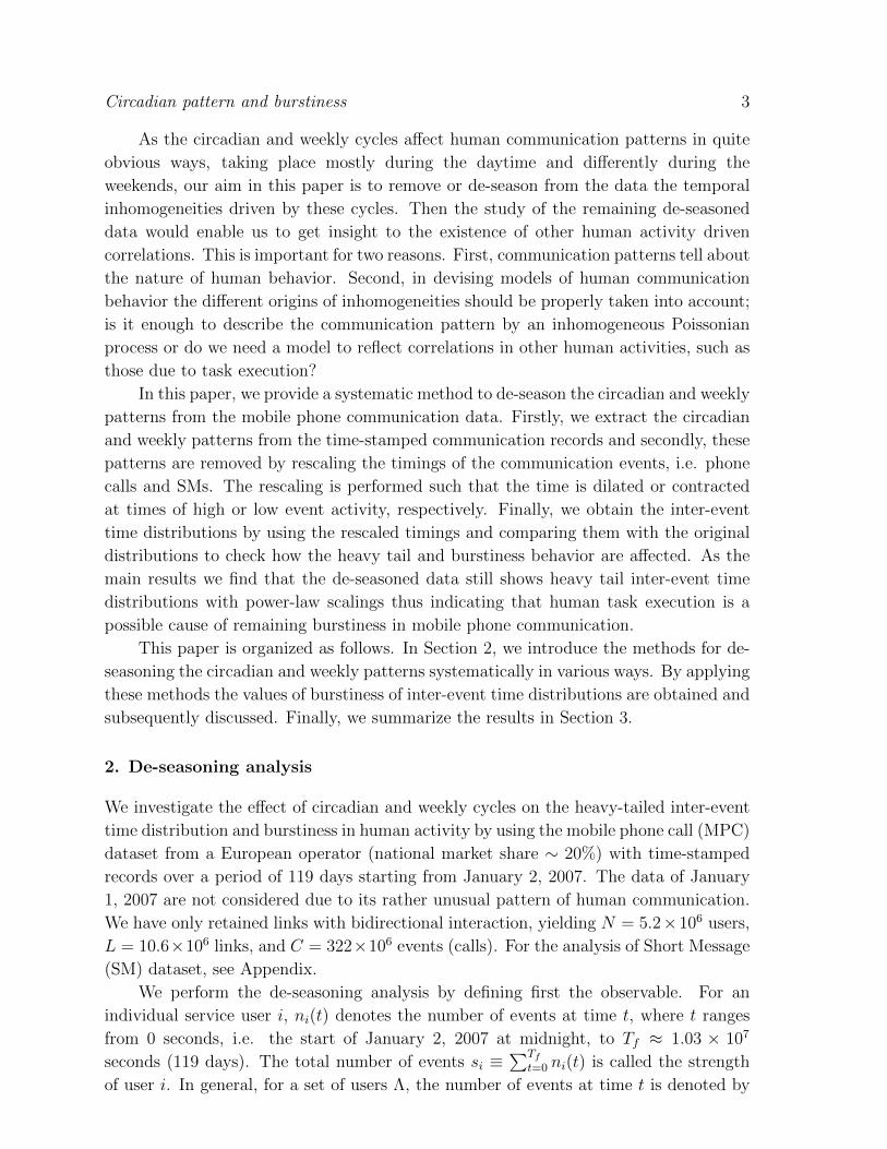
Figure 1. De-seasoning MPC patterns of individual users: the original and the
rescaled event rates with period of T = 1 day (left) and the original and the rescaled
inter-event time distributions with various periods of T (right). Individual users with
the strength si = 200 (a), 400 (b), 800 (c), 1600 (d), and 3197 (e) are analyzed. The
original inter-event time distribution of the whole population is also plotted as a dashed
curve for comparison.
rescaled event rates. The event rates in case of T = 1 day are depicted in the left
column of Fig. 1. The strengths of individual users are 200, 400, 800, 1600, and 3197.
In most cases we find the characteristic circadian pattern, i.e. inactive nighttime and
active daytime with one peak in the afternoon and another peak in the evening. The
rescaled event rate successfully shows the expected de-seasoning effect, i.e. ρ∗(t∗) = 1,
except for weak fluctuations.
The rescaled inter-event time distributions up to T = 28 days are compared with

Circadian pattern and burstiness 6
0
0.02
0.04
0.06
0.08
0.1
-0.4 -0.2 0 0.2 0.4 0.6 0.8 1
P(B
T)
BT
(a)original
T=1 day28 days
0
0.1
0.2
0.3
0.4
0.5
-0.6 -0.5 -0.4 -0.3 -0.2 -0.1 0 0.1 0.2
P(∆BT)
∆BT
T=1 day28 days
0
0.04
0.08
0.12
-0.4 -0.2 0 0.2 0.4 0.6 0.8 1
P(B
T)
BT
(b)original
T=1 day28 days
0
0.1
0.2
0.3
0.4
-0.6 -0.5 -0.4 -0.3 -0.2 -0.1 0 0.1 0.2
P(∆BT)
∆BT
T=1 day28 days
0
0.04
0.08
0.12
0.16
-0.4 -0.2 0 0.2 0.4 0.6 0.8 1
P(B
T)
BT
(c)original
T=1 day28 days
0
0.1
0.2
0.3
-0.6 -0.5 -0.4 -0.3 -0.2 -0.1 0 0.1 0.2
P(∆BT)
∆BT
T=1 day28 days
0
0.1
0.2
0.3
-0.4 -0.2 0 0.2 0.4 0.6 0.8 1
P(B
T)
BT
(d)original
T=1 day28 days
0
0.1
0.2
0.3
-0.6 -0.5 -0.4 -0.3 -0.2 -0.1 0 0.1 0.2
P(∆BT)
∆BT
T=1 day28 days
Figure 2. Distributions P (BT ) of the original and rescaled burstiness of invididual
users with the same strength (left) and distributions P (∆BT ) of the difference in
burstiness, defined as ∆BT = BT −B0 (right). The individual users with the strengths
si = 200 (a), 400 (b), 800 (c), and 1600 (d) are analyzed. The numbers of users are
correspondingly 6397, 1746, 196, and 7.
the original distributions in the right column of Fig. 1. Note that the possible minimum
value of rescaled inter-event time is T/si. We find that the rescaled inter-event time
distributions still show the heavy tails. For the user with strength 200, the burstiness
decreases from the original value of B0 ≈ 0.202 to value B7 ≈ 0.174 (weekly pattern
removed), then dropping further to value B28 ≈ 0.104 (i.e. monthly pattern removed).
For the most active user with strength si = 3197, the burstiness decays faster as T
increases: B0 ≈ 0.469, B7 ≈ 0.254, and B28 ≈ 0.219. However, the values of B are
overall larger than those of the less active user. The results imply that de-seasoning
the circadian and weekly patterns does not considerably affect the temporal burstiness
patterns of individuals. Finally, in a limiting case of T = Tf , since ni(t) has the value
of either 0 or 1, all τ ∗ are the same as T/si in Eqs. (1) and (3), leading to BTf = −1.
Next, we obtain the distributions P (BT ) of original and rescaled values of burstiness
of individual users with the same strength and the distributions P (∆BT ) of the difference
Circadian pattern and burstiness 7
-0.2
-0.1
0
0.1
0.2
0.3
0.4
0.5
0.6
0.7
orig. 1 2 4 7 14 28 56
BT
T (days)
(a)s=1600s=800s=400s=200
0.2
0.25
0.3
0.35
0.4
orig. 1 2 4 7 14 28 56
BT
T (days)
(b)s=1600s=800s=400s=200
0.2
0.3
0.4
0.5
0.6
0.7
orig. 1 2 4 7 14 28 56
BT
T (days)
(c)whole
group 6531
Figure 3. Burstiness BT as a function of period of T : (a) the average and the standard
deviation of BT obtained from the burstiness distribution in Fig. 2, (b) burstiness from
groups with the same strength, and (c) burstiness from groups with broad ranges of
strength.
in burstiness, defined as ∆BT ≡ BT − B0, see Fig. 2. The averages and the standard
deviations of burstiness distributions for different periods of T are plotted in Fig. 3(a).
The more active users have the larger values of burstiness, while the values of burstiness
of the more active users decays faster (slower) than those of the less active users before
(after) T = 7 days. The overall behavior of the distributions shows that de-seasoning the
circadian and weekly patterns does not destroy the bursty behavior of most individual
users irrespective of their strengths. In addition, we find some exceptional users whose
original values of burstiness are negative, indicating for more regular behavior than the
Poisson process, and we also find a few individual users whose values of burstiness have
grown as a result of de-seasoning, i.e. ∆BT > 0.
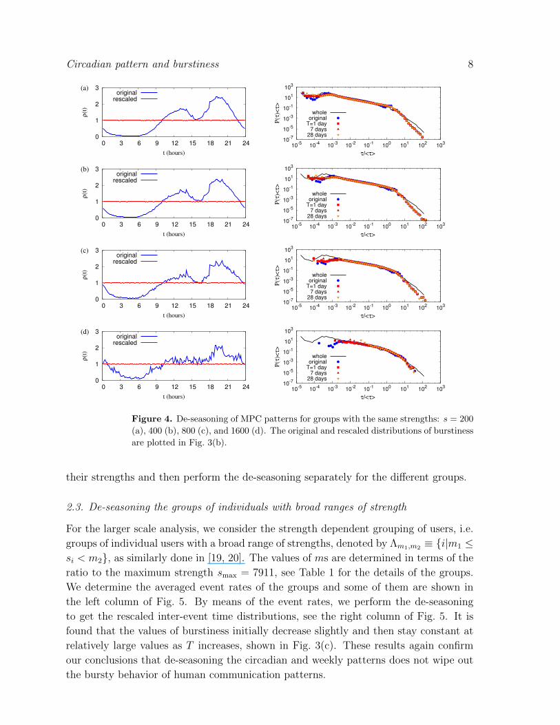
2.2. De-seasoning the groups of individuals with the same strength
Here we analyze the group of individual users with the same strength, i.e. Λs ≡ {i|si =
s}. The averaged event rate of a group is measured by merging individual event rates,
precisely by obtaining nΛs(t) =∑
i∈Λsni(t). Figure 4 shows the original and the rescaled
event rates with T = 1 day (left) and the original and the rescaled inter-event time
distributions with various periods of T (right) for groups with strengths s = 200, 400,
800, and 1600. The values of burstiness decrease only slightly as T increases, but are
smaller than those of the original burstiness, as shown in Fig. 3(b).
The burstiness of groups of individuals with the same strength is larger than
the average values of individual burstiness from P (B) of the same strength. For
example, B0 ≈ 0.256 for the group of strength s = 200 turns out to be larger
than∫P (B0)dB0 ≈ 0.204. Regarding to this difference, we would like to note that
the de-seasoning of individual event times by means of the averaged event rate may
cause systematic errors due to the different circadian and weekly patterns between the
individual and the group. For resolving this issue, the various data clustering methods,
such as self-organizing maps, can be used to classify users’ activity patterns beyond
Circadian pattern and burstiness 8
0
1
2
3
0 3 6 9 12 15 18 21 24
ρ(t
)
t (hours)
(a)original
rescaled
10-7
10-5
10-3
10-1
101
103
10-5
10-4
10-3
10-2
10-1
100
101
102
103
P(τ
)<τ>
τ/<τ>
wholeoriginal
T=1 day7 days
28 days
0
1
2
3
0 3 6 9 12 15 18 21 24
ρ(t
)
t (hours)
(b)original
rescaled
10-7
10-5
10-3
10-1
101
103
10-5
10-4
10-3
10-2
10-1
100
101
102
103
P(τ
)<τ>
τ/<τ>
wholeoriginal
T=1 day7 days
28 days
0
1
2
3
0 3 6 9 12 15 18 21 24
ρ(t
)
t (hours)
(c)original
rescaled
10-7
10-5
10-3
10-1
101
103
10-5
10-4
10-3
10-2
10-1
100
101
102
103
P(τ
)<τ>
τ/<τ>
wholeoriginal
T=1 day7 days
28 days
0
1
2
3
0 3 6 9 12 15 18 21 24
ρ(t
)
t (hours)
(d)original
rescaled
10-7
10-5
10-3
10-1
101
103
10-5
10-4
10-3
10-2
10-1
100
101
102
103
P(τ
)<τ>
τ/<τ>
wholeoriginal
T=1 day7 days
28 days
Figure 4. De-seasoning of MPC patterns for groups with the same strengths: s = 200
(a), 400 (b), 800 (c), and 1600 (d). The original and rescaled distributions of burstiness
are plotted in Fig. 3(b).
their strengths and then perform the de-seasoning separately for the different groups.
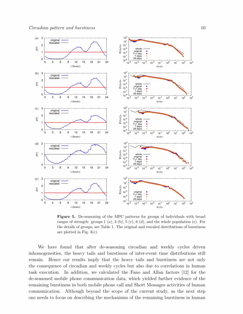
2.3. De-seasoning the groups of individuals with broad ranges of strength
For the larger scale analysis, we consider the strength dependent grouping of users, i.e.
groups of individual users with a broad range of strengths, denoted by Λm1,m2 ≡ {i|m1 ≤si < m2}, as similarly done in [19, 20]. The values of ms are determined in terms of the
ratio to the maximum strength smax = 7911, see Table 1 for the details of the groups.
We determine the averaged event rates of the groups and some of them are shown in
the left column of Fig. 5. By means of the event rates, we perform the de-seasoning
to get the rescaled inter-event time distributions, see the right column of Fig. 5. It is
found that the values of burstiness initially decrease slightly and then stay constant at
relatively large values as T increases, shown in Fig. 3(c). These results again confirm
our conclusions that de-seasoning the circadian and weekly patterns does not wipe out
the bursty behavior of human communication patterns.
Circadian pattern and burstiness 9
Table 1. Strength dependent grouping of individuals in the MPC dataset. For each
group, the range of strength, also in terms of the ratio to the maximum strength
smax = 7911, the number of users, and its fraction to the whole population except for
the user with smax are summarized.group index strength range (%) the number of users (%)
0 0-79 (0-1) 2821103 (54.4)
1 79-158 (1-2) 1010923 (19.5)
2 158-316 (2-4) 843412 (16.3)
3 316-632 (4-8) 418460 (8.1)
4 632-1265 (8-16) 89718 (1.7)
5 1265-2531 (16-32) 5857 (0.1)
6 2531-5063 (32-64) 173 (0.003)
7 5063-7594 (64-96) 5 (0.0001)
whole 0-7594 (0-96) 5189651 (100)
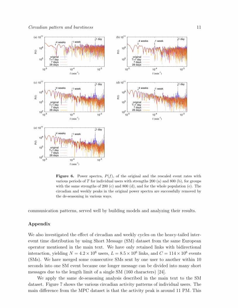
2.4. Power spectra analysis
In order to see clearly the effect of de-seasoning on the event rates, we compare the power
spectra of the rescaled event rates to the original event rates. The power spectrum of
the event rate is defined as
P (f) =
∣∣∣∣∣∣Tf∑t=0
ρΛ,T (t)e2πift
∣∣∣∣∣∣2
, (5)
where f denotes the frequency. In Fig. 6 we show the results of this comparison,
where it is evident that with our de-seasoning methods, the circadian and weekly
peaks of the original power spectrum are successfully removed and do not show in the
rescaled spectra. In all the cases, ranging from the individual de-seasoning to the whole
population de-seasoning, when T = 1 day, the circadian peak at 1/f = 1 day is removed
while the others, i.e. the weekly and monthly peaks remain. For T = 7 days, the weekly
peak at 1/f = 7 days is removed, and so on. This behavior can be understood because
the cyclic patterns longer than T will not be affected by de-seasoning with the period
T .
3. Summary
The heavy tails and burstiness of inter-event time distributions in human communication
activity are affected by circadian and weekly cycles as well as by correlations rooted in
human task execution. To investigate the existence of correlations rooted in human task
execution we devised a systematic method to de-season circadian and weekly cycles
appearing in human activity and successfully demonstrated their removal. Here the
circadian and weekly patterns extracted from the mobile phone call and Short Messages
records are used to rescale the timings of events, i.e. the time is dilated or contracted
during high or low call or SM activity of individual service users, respectively.
Circadian pattern and burstiness 10
0
1
2
3
0 3 6 9 12 15 18 21 24
ρ(t
)
t (hours)
(a)original
rescaled
10-9
10-7
10-5
10-3
10-1
101
103
10-5
10-4
10-3
10-2
10-1
100
101
102
103
P(τ
)<τ>
τ/<τ>
wholeoriginal
T=1 day7 days
28 days
0
1
2
3
0 3 6 9 12 15 18 21 24
ρ(t
)
t (hours)
(b)original
rescaled
10-9
10-7
10-5
10-3
10-1
101
103
10-5
10-4
10-3
10-2
10-1
100
101
102
103
P(τ
)<τ>
τ/<τ>
wholeoriginal
T=1 day7 days
28 days
0
1
2
3
0 3 6 9 12 15 18 21 24
ρ(t
)
t (hours)
(c)original
rescaled
10-9
10-7
10-5
10-3
10-1
101
103
10-5
10-4
10-3
10-2
10-1
100
101
102
103
P(τ
)<τ>
τ/<τ>
wholeoriginal
T=1 day7 days
28 days
0
1
2
0 3 6 9 12 15 18 21 24
ρ(t
)
t (hours)
(d)original
rescaled
10-9
10-7
10-5
10-3
10-1
101
103
10-5
10-4
10-3
10-2
10-1
100
101
102
103
P(τ
)<τ>
τ/<τ>
wholeoriginal
T=1 day7 days
28 days
0
1
2
3
0 3 6 9 12 15 18 21 24
ρ(t
)
t (hours)
(e)original
rescaled
10-7
10-5
10-3
10-1
101
103
10-5
10-4
10-3
10-2
10-1
100
101
102
103
P(τ
)<τ>
τ/<τ>
originalT=1 day
7 days28 days
Figure 5. De-seasoning of the MPC patterns for groups of individuals with broad
ranges of strength: groups 1 (a), 3 (b), 5 (c), 6 (d), and the whole population (e). For
the details of groups, see Table 1. The original and rescaled distributions of burstiness
are plotted in Fig. 3(c).
We have found that after de-seasoning circadian and weekly cycles driven
inhomogeneities, the heavy tails and burstiness of inter-event time distributions still
remain. Hence our results imply that the heavy tails and burstiness are not only
the consequence of circadian and weekly cycles but also due to correlations in human
task execution. In addition, we calculated the Fano and Allan factors [12] for the
de-seasoned mobile phone communication data, which yielded further evidence of the
remaining burstiness in both mobile phone call and Short Messages activities of human
communication. Although beyond the scope of the current study, as the next step
one needs to focus on describing the mechanisms of the remaining burstiness in human
Circadian pattern and burstiness 11
105
108
1011
10-5
10-4
10-3
P(f
)
f (min-1
)
(a)1 day
1 week4 weeks
originalT=1 day
7 days28 days
105
108
1011
10-5
10-4
10-3
P(f
)
f (min-1
)
(b)1 day
1 week4 weeks
originalT=1 day
7 days28 days
102
105
108
1011
10-5
10-4
10-3
P(f
)
f (min-1
)
(c)1 day
1 week4 weeks
originalT=1 day
7 days28 days
102
105
108
1011
10-5
10-4
10-3
P(f
)f (min
-1)
(d)1 day
1 week4 weeks
originalT=1 day
7 days28 days
102
105
108
1011
10-5
10-4
10-3
P(f
)
f (min-1
)
(e)1 day
1 week4 weeks
originalT=1 day
7 days28 days
Figure 6. Power spectra, P (f), of the original and the rescaled event rates with
various periods of T for individual users with strengths 200 (a) and 800 (b), for groups
with the same strengths of 200 (c) and 800 (d), and for the whole population (e). The
circadian and weekly peaks in the original power spectra are successfully removed by
the de-seasoning in various ways.
communication patterns, served well by building models and analyzing their results.
Appendix
We also investigated the effect of circadian and weekly cycles on the heavy-tailed inter-
event time distribution by using Short Message (SM) dataset from the same European
operator mentioned in the main text. We have only retained links with bidirectional
interaction, yielding N = 4.2× 10⁶ users, L = 8.5× 10⁶ links, and C = 114× 106 events
(SMs). We have merged some consecutive SMs sent by one user to another within 10
seconds into one SM event because one longer message can be divided into many short
messages due to the length limit of a single SM (160 characters) [24].
We apply the same de-seasoning analysis described in the main text to the SM
dataset. Figure 7 shows the various circadian activity patterns of individual users. The
main difference from the MPC dataset is that the activity peak is around 11 PM. This

Circadian pattern and burstiness 12
0
3
6
9
12
0 3 6 9 12 15 18 21 24
ρ(t
)
t (hours)
(a)original
rescaled
10-5
10-3
10-1
101
103
10-5
10-4
10-3
10-2
10-1
100
101
102
P(τ
)<τ>
τ/<τ>
wholeoriginal
T=1 day7 days
28 days
0
1
2
3
4
5
6
0 3 6 9 12 15 18 21 24
ρ(t
)
t (hours)
(b)original
rescaled
10-5
10-3
10-1
101
103
10-5
10-4
10-3
10-2
10-1
100
101
102
P(τ
)<τ>
τ/<τ>
wholeoriginal
T=1 day7 days
28 days
0
1
2
3
4
5
0 3 6 9 12 15 18 21 24
ρ(t
)
t (hours)
(c)original
rescaled
10-5
10-3
10-1
101
103
10-5
10-4
10-3
10-2
10-1
100
101
102
P(τ
)<τ>
τ/<τ>
wholeoriginal
T=1 day7 days
28 days
0
1
2
3
0 3 6 9 12 15 18 21 24
ρ(t
)
t (hours)
(d)original
rescaled
10-5
10-3
10-1
101
103
10-5
10-4
10-3
10-2
10-1
100
101
102
P(τ
)<τ>
τ/<τ>
wholeoriginal
T=1 day7 days
28 days
0
1
2
3
0 3 6 9 12 15 18 21 24
ρ(t
)
t (hours)
(e)original
rescaled
10-5
10-3
10-1
101
103
10-5
10-4
10-3
10-2
10-1
100
101
102
P(τ
)<τ>
τ/<τ>
wholeoriginal
T=1 day7 days
28 days
Figure 7. De-seasoning SM patterns of individual users: the original and the rescaled
event rates with period of T = 1 day (left) and the original and the rescaled inter-event
time distributions with various periods of T (right). Individual users with the strength
si = 200 (a), 400 (b), 800 (c), 1600 (d), and 3200 (e) are analyzed. The original
inter-event time distribution of the whole population is also plotted as a dashed curve
for comparison.
feature becomes evident if the averaged event rates are obtained from the same strength
groups or from the groups with broad ranges of strength, shown in the left columns of
Figs 10 and 11. For the details of the strength dependent grouping, see Table 2.
The inter-event time distributions and their values of burstiness are also compared.
At first, the distributions cannot be described by the simple power-law form but by the
bimodal combination of power-law and Poisson distributions as suggested by [23]. As
shown in Fig. 9, the values of burstiness slowly decrease as the period T increases up

Circadian pattern and burstiness 13
0
0.02
0.04
0.06
0.08
-0.4 -0.2 0 0.2 0.4 0.6 0.8 1
P(B
T)
BT
(a)original
T=1 day28 days
0
0.2
0.4
0.6
0.8
1
-0.6 -0.5 -0.4 -0.3 -0.2 -0.1 0 0.1 0.2
P(∆BT)
∆BT
T=1 day28 days
0
0.02
0.04
0.06
0.08
-0.4 -0.2 0 0.2 0.4 0.6 0.8 1
P(B
T)
BT
(b)original
T=1 day28 days
0 0.1 0.2 0.3 0.4 0.5 0.6 0.7
-0.6 -0.5 -0.4 -0.3 -0.2 -0.1 0 0.1 0.2
P(∆BT)
∆BT
T=1 day28 days
0
0.02
0.04
0.06
0.08
0.1
-0.4 -0.2 0 0.2 0.4 0.6 0.8 1
P(B
T)
BT
(c)original
T=1 day28 days
0
0.1
0.2
0.3
0.4
0.5
-0.6 -0.5 -0.4 -0.3 -0.2 -0.1 0 0.1 0.2
P(∆BT)
∆BT
T=1 day28 days
0
0.1
0.2
-0.4 -0.2 0 0.2 0.4 0.6 0.8 1
P(B
T)
BT
(d)original
T=1 day28 days
0
0.1
0.2
0.3
-0.6 -0.5 -0.4 -0.3 -0.2 -0.1 0 0.1 0.2
P(∆BT)
∆BT
T=1 day28 days
Figure 8. Distributions P (BT ) of the original and rescaled burstiness of invididual
users with the same strength (left) and distributions P (∆BT ) of the difference in
burstiness, defined as ∆BT = BT −B0 (right). The individual users with the strengths
si = 200 (a), 400 (b), 800 (c), and 1600 (d) are analyzed. The numbers of users are
correspondingly 1434, 344, 62, and 10.
-0.1
0
0.1
0.2
0.3
0.4
0.5
0.6
0.7
0.8
0.9
orig. 1 2 4 7 14 28 56
BT
T (days)
(a)s=1600s=800s=400s=200
0.35
0.4
0.45
0.5
0.55
0.6
orig. 1 2 4 7 14 28 56
BT
T (days)
(b)s=1600s=800s=400s=200
0.3
0.4
0.5
0.6
0.7
0.8
0.9
orig. 1 2 4 7 14 28 56
BT
T (days)
(c)whole
group 7531
Figure 9. Burstiness BT as a function of period of T : (a) the average and the standard
deviation of BT obtained from the burstiness distribution in Fig. 8, (b) burstiness from
groups with the same strength, and (c) burstiness from groups with broad ranges of
strength.
Circadian pattern and burstiness 14
0
1
2
0 3 6 9 12 15 18 21 24
ρ(t
)
t (hours)
(a)original
rescaled
10-7
10-5
10-3
10-1
101
103
10-5
10-4
10-3
10-2
10-1
100
101
102
103
P(τ
)<τ>
τ/<τ>
wholeoriginal
T=1 day7 days
28 days
0
1
2
3
0 3 6 9 12 15 18 21 24
ρ(t
)
t (hours)
(b)original
rescaled
10-7
10-5
10-3
10-1
101
103
10-5
10-4
10-3
10-2
10-1
100
101
102
103
P(τ
)<τ>
τ/<τ>
wholeoriginal
T=1 day7 days
28 days
0
1
2
3
0 3 6 9 12 15 18 21 24
ρ(t
)
t (hours)
(c)original
rescaled
10-7
10-5
10-3
10-1
101
103
10-5
10-4
10-3
10-2
10-1
100
101
102
103
P(τ
)<τ>
τ/<τ>
wholeoriginal
T=1 day7 days
28 days
0
1
2
3
4
0 3 6 9 12 15 18 21 24
ρ(t
)
t (hours)
(d)original
rescaled
10-7
10-5
10-3
10-1
101
103
10-5
10-4
10-3
10-2
10-1
100
101
102
103
P(τ
)<τ>
τ/<τ>
wholeoriginal
T=1 day7 days
28 days
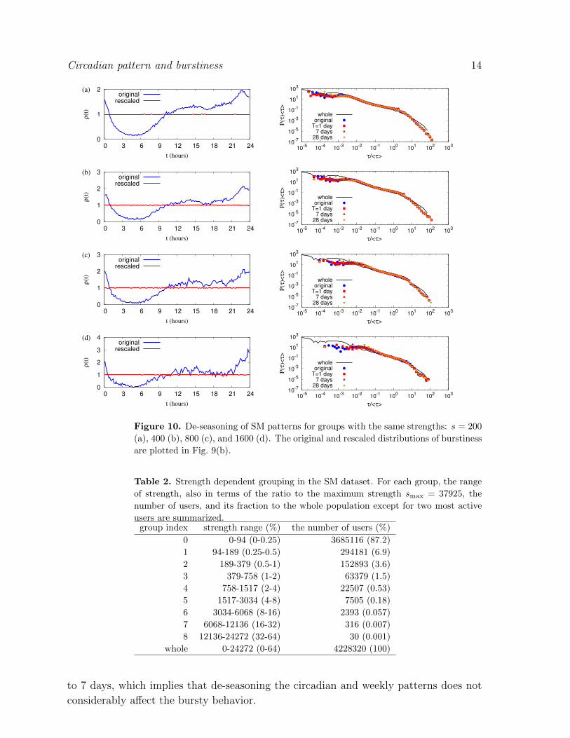
Figure 10. De-seasoning of SM patterns for groups with the same strengths: s = 200
(a), 400 (b), 800 (c), and 1600 (d). The original and rescaled distributions of burstiness
are plotted in Fig. 9(b).
Table 2. Strength dependent grouping in the SM dataset. For each group, the range
of strength, also in terms of the ratio to the maximum strength smax = 37925, the
number of users, and its fraction to the whole population except for two most active
users are summarized.group index strength range (%) the number of users (%)
0 0-94 (0-0.25) 3685116 (87.2)
1 94-189 (0.25-0.5) 294181 (6.9)
2 189-379 (0.5-1) 152893 (3.6)
3 379-758 (1-2) 63379 (1.5)
4 758-1517 (2-4) 22507 (0.53)
5 1517-3034 (4-8) 7505 (0.18)
6 3034-6068 (8-16) 2393 (0.057)
7 6068-12136 (16-32) 316 (0.007)
8 12136-24272 (32-64) 30 (0.001)
whole 0-24272 (0-64) 4228320 (100)
to 7 days, which implies that de-seasoning the circadian and weekly patterns does not
considerably affect the bursty behavior.

Circadian pattern and burstiness 15
0
1
2
0 3 6 9 12 15 18 21 24
ρ(t
)
t (hours)
(a)original
rescaled
10-9
10-7
10-5
10-3
10-1
101
103
10-5
10-4
10-3
10-2
10-1
100
101
102
103
P(τ
)<τ>
τ/<τ>
wholeoriginal
T=1 day7 days
28 days
0
1
2
3
0 3 6 9 12 15 18 21 24
ρ(t
)
t (hours)
(b)original
rescaled
10-9
10-7
10-5
10-3
10-1
101
103
10-5
10-4
10-3
10-2
10-1
100
101
102
103
P(τ
)<τ>
τ/<τ>
wholeoriginal
T=1 day7 days
28 days
0
1
2
3
0 3 6 9 12 15 18 21 24
ρ(t
)
t (hours)
(c)original
rescaled
10-9
10-7
10-5
10-3
10-1
101
103
10-5
10-4
10-3
10-2
10-1
100
101
102
103
P(τ
)<τ>
τ/<τ>
wholeoriginal
T=1 day7 days
28 days
0
1
2
3
0 3 6 9 12 15 18 21 24
ρ(t
)
t (hours)
(d)original
rescaled
10-9
10-7
10-5
10-3
10-1
101
103
10-5
10-4
10-3
10-2
10-1
100
101
102
103
P(τ
)<τ>
τ/<τ>
wholeoriginal
T=1 day7 days
28 days
0
1
2
0 3 6 9 12 15 18 21 24
ρ(t
)
t (hours)
(e)original
rescaled
10-5
10-3
10-1
101
103
10-5
10-4
10-3
10-2
10-1
100
101
102
P(τ
)<τ>
τ/<τ>
originalT=1 day
7 days28 days
Figure 11. De-seasoning of the SM patterns for groups of individuals with broad
ranges of strength: groups 1 (a), 3 (b), 5 (c), 7 (d), and the whole population (e). For
the details of groups, see Table 2. The original and rescaled distributions of burstiness
are plotted in Fig. 9(c).
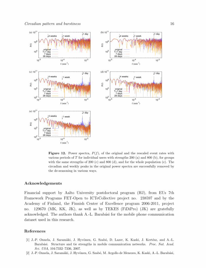
Finally, we perform the power spectrum analysis for SM dataset in Fig. 12 and find
again that the cyclic patterns longer than T cannot be removed by the de-seasoning with
period T . All these results confirm our conclusion that the heavy tail and burstiness
are not only the consequence of circadian and other longer cycle patterns but also due
to other correlations, such as human task execution.
Circadian pattern and burstiness 16
105
108
1011
10-5
10-4
10-3
P(f
)
f (min-1
)
(a)1 day
1 week4 weeks
originalT=1 day
7 days28 days
105
108
1011
10-5
10-4
10-3
P(f
)
f (min-1
)
(b)1 day
1 week4 weeks
originalT=1 day
7 days28 days
102
105
108
1011
10-5
10-4
10-3
P(f
)
f (min-1
)
(c)1 day
1 week4 weeks
originalT=1 day
7 days28 days
102
105
108
1011
10-5
10-4
10-3
P(f
)f (min
-1)
(d)1 day
1 week4 weeks
originalT=1 day
7 days28 days
102
105
108
1011
10-5
10-4
10-3
P(f
)
f (min-1
)
(e)1 day
1 week4 weeks
originalT=1 day
7 days28 days
Figure 12. Power spectra, P (f), of the original and the rescaled event rates with
various periods of T for individual users with strengths 200 (a) and 800 (b), for groups
with the same strengths of 200 (c) and 800 (d), and for the whole population (e). The
circadian and weekly peaks in the original power spectra are successfully removed by
the de-seasoning in various ways.
Acknowledgements
Financial support by Aalto University postdoctoral program (HJ), from EUs 7th
Framework Programs FET-Open to ICTeCollective project no. 238597 and by the
Academy of Finland, the Finnish Center of Excellence program 2006-2011, project
no. 129670 (MK, KK, JK), as well as by TEKES (FiDiPro) (JK) are gratefully
acknowledged. The authors thank A.-L. Barabasi for the mobile phone communication
dataset used in this research.
References
[1] J.-P. Onnela, J. Saramaki, J. Hyvonen, G. Szabo, D. Lazer, K. Kaski, J. Kertesz, and A.-L.
Barabasi. Structure and tie strengths in mobile communication networks. Proc. Nat. Acad.
Sci. USA, 104:7332–7336, 2007.
[2] J.-P. Onnela, J. Saramaki, J. Hyvonen, G. Szabo, M. Argollo de Menezes, K. Kaski, A.-L. Barabasi,
Circadian pattern and burstiness 17
and J. Kertesz. Analysis of a large-scale weighted network of one-to-one human communication.
New J. Phys., 9:179, 2007.
[3] G. Krings, F. Calabrese, C. Ratti, and V. D. Blondel. Urban gravity: a model for inter-city
telecommunication flows. Journal of Statistical Mechanics, 2009:L07003, 2009.
[4] G. Palla, A.-L. Barabasi, and T. Vicsek. Quantifying social group evolution. Nature, 446:664–667,
2007.
[5] M. C. Gonzalez, C. A. Hidalgo, and A.-L. Barabasi. Understanding individual human mobility
patterns. Nature, 453:779–782, 2008.
[6] C. Song, Z. Qu, N. Blumm, and A.-L. Barabasi. Limits of predictability in human mobility.
Science, 327:1018–1021, 2010.
[7] C. Song, T. Koren, P. Wang, and A.-L. Barabasi. Modelling the scaling properties of human
mobility. Nature Physics, 6:818–823, 2010.
[8] A.-L. Barabasi. The origin of bursts and heavy tails in human dynamics. Nature, 435:207–211,
2005.
[9] R. D. Malmgren, D. B. Stouffer, A. E. Motter, and L. A. N. Amaral. A poissonian explanation
for heavy tails in e-mail communication. Proc. Nat. Acad. Sci. USA, 105:18153–18158, 2008.
[10] R. D. Malmgren, D. B. Stouffer, A. S. L. O. Campanharo, and L. A. N. Amaral. On universality
in human correspondence activity. Science, 325:1696–1700, 2009.
[11] R. D. Malmgren, J. M. Hofman, L. A. N. Amaral, and D. J. Watts. Characterizing individual
communication patterns. In KDD ’09: Proceedings of the 15th ACM SIGKDD international
conference on Knowledge discovery and data mining, pages 607–616, New York, NY, USA, 2009.
ACM Press.
[12] C. Anteneodo, R. D. Malmgren, and D. R. Chialvo. Poissonian bursts in e-mail correspondence.
Eur. Phys. J. B, 2010.
[13] G. Miritello, E. Moro, and R. Lara. Dynamical strength of social ties in information spreading.
Phys. Rev. E, 83:045102, 2011.
[14] M. Karsai, M. Kivela, R. K. Pan, K. Kaski, J. Kertesz, A.-L. Barabasi, and J. Saramaki. Small
but slow world: How network topology and burstiness slow down spreading. Phys. Rev. E,
83:025102, 2011.
[15] A. Johansen. Response time of internauts. Physica A, 296:539–546, 2001.
[16] J.-P. Eckmann, E. Moses, and D. Sergi. Entropy of dialogues creates coherent structures in e-mail
traffic. Proc. Nat. Acad. Sci. USA, 101:14333–14337, 2004.
[17] U. Harder and M. Paczuski. Correlated dynamics in human printing behavior. Physica A, 361:329–
336, 2006.
[18] B. Goncalves and J. J. Ramasco. Human dynamics revealed through web analytics. Phys. Rev.
E, 78:026123, 2008.
[19] T. Zhou, H. A. T. Kiet, B. J. Kim, B. H. Wang, and P. Holme. Role of activity in human dynamics.
EPL (Europhysics Letters), 82:28002, 2008.
[20] F. Radicchi. Human activity in the web. Phys. Rev. E, 80:026118, 2009.
[21] A. Vazquez, J. G. Oliveira, Z. Dezso, K.-I. Goh, I. Kondor, and A.-L. Barabasi. Modeling bursts
and heavy tails in human dynamics. Phys. Rev. E, 73:036127, 2006.
[22] K.-I. Goh and A.-L. Barabasi. Burstiness and memory in complex systems. EPL (Europhysics
Letters), 81:48002, 2008.
[23] Y. Wu, C. Zhou, J. Xiao, J. Kurths, and H. J. Schellnhuber. Evidence for a bimodal distribution
in human communication. Proc. Nat. Acad. Sci. USA, 107:18803–18808, 2010.
[24] L. Kovanen. Structure and dynamics of a large-scale complex social network. Master’s thesis,
Aalto University, Espoo, Finland, 2009.