Chp.5 Optimum Consumption and Portfolio Rules in a Continuous Time
Model
Hai Lin
Department of Finance, Xiamen University

1. Introduction
• In chp.4,the continuous time consumption portfolio problem for an individual whose income is generated by capital gains in assets with geometric Brownian Motion hypothesis is analyzed, and some special cases, such as the constant relative and absolute risk aversion are considered and solved explicitly.
• Common hypothesis about the behavior of asset prices: random walk of returns or geometric Brownian Motion hypothesis. Some questioned the accuracy of this.Cootner(1964), Mandelbrot(1963a,b), and Fama(1965). The nonacademic literature is technical analysis or charting.
• This chapter extends the results of last chapter for more general utilities functions, price behavior assumptions, and income generated from other non capital gain.

Main conclusions
• Some conclusions:– If the geometric Brownian Motion hypothesis is accept
ed, then a general separation or mutual fund theorem can be proved, and the classical Markowitz-Tobin mean-variance rules hold without the utility function and the distribution of asset prices.
– If further assumption is made called HARA, explicit solutions are derived.
– The effects on the consumption and portfolio rules of alternative asset price dynamics, are examined with the wage income, uncertainty of life expectancy, and the possibility of default on risk free assets.
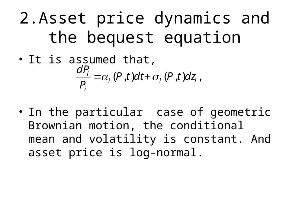
2.Asset price dynamics and the bequest equation
• It is assumed that,
• In the particular case of geometric Brownian motion, the conditional mean and volatility is constant. And asset price is log-normal.
,),(),( iiii
i dztPdttPP
dP
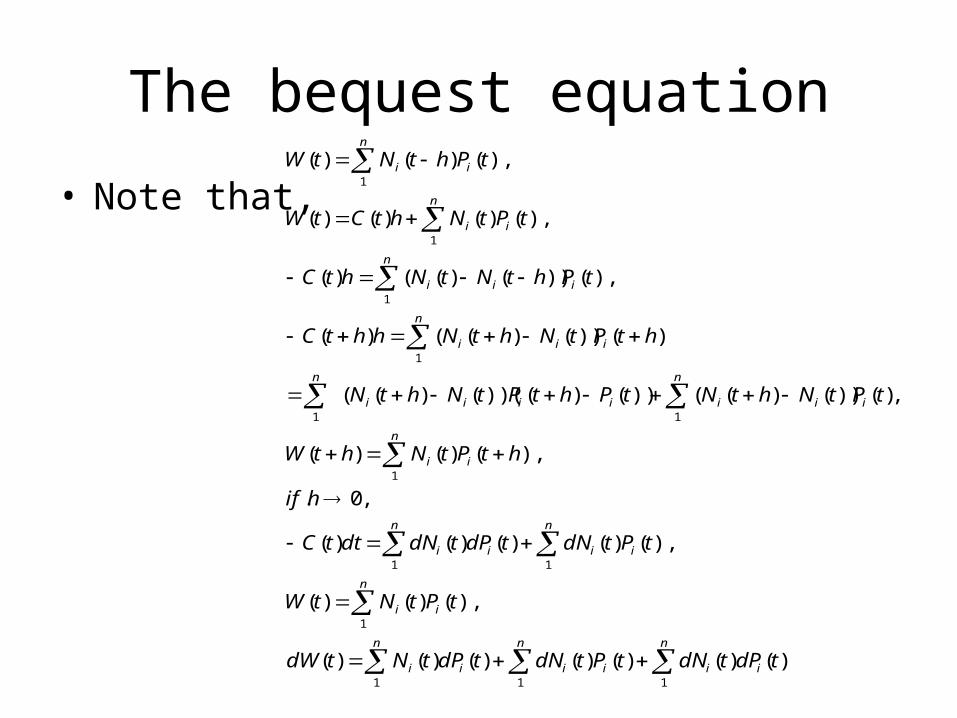
The bequest equation
• Note that,
n n n
iiiiii
n
ii
n n
iiii
n
ii
n
iiiiiii
n
n
iii
n
iii
n
ii
n
ii
tdPtdNtPtdNtdPtNtdW
tPtNtW
tPtdNtdPtdNdttC
hif
htPtNhtW
tPtNhtNtPhtPtNhtN
htPtNhtNhhtC
tPhtNtNhtC
tPtNhtCtW
tPhtNtW
1 1 1
1
1 1
1
11
1
1
1
1
)()()()()()()(
),()()(
),()()()()(
,0.
),()()(
,)())()(())()())(()((
)())()(()(
),())()(()(
),()()()(
),()()(

Considering the non-capital gain
n
i
n
iii
n
ii
n
iii
iii
n
ii
n n
iiii
wts
dzWwdyCdtdydtWw
CdtdyPWdPwdW
tWtPtNtw
dttCdytdPtN
tPtdNtdPtdNdttCdy
1
11
1
1
1 1
.1..
,
/
),(/)()()(
,)()()(
)()()()()(
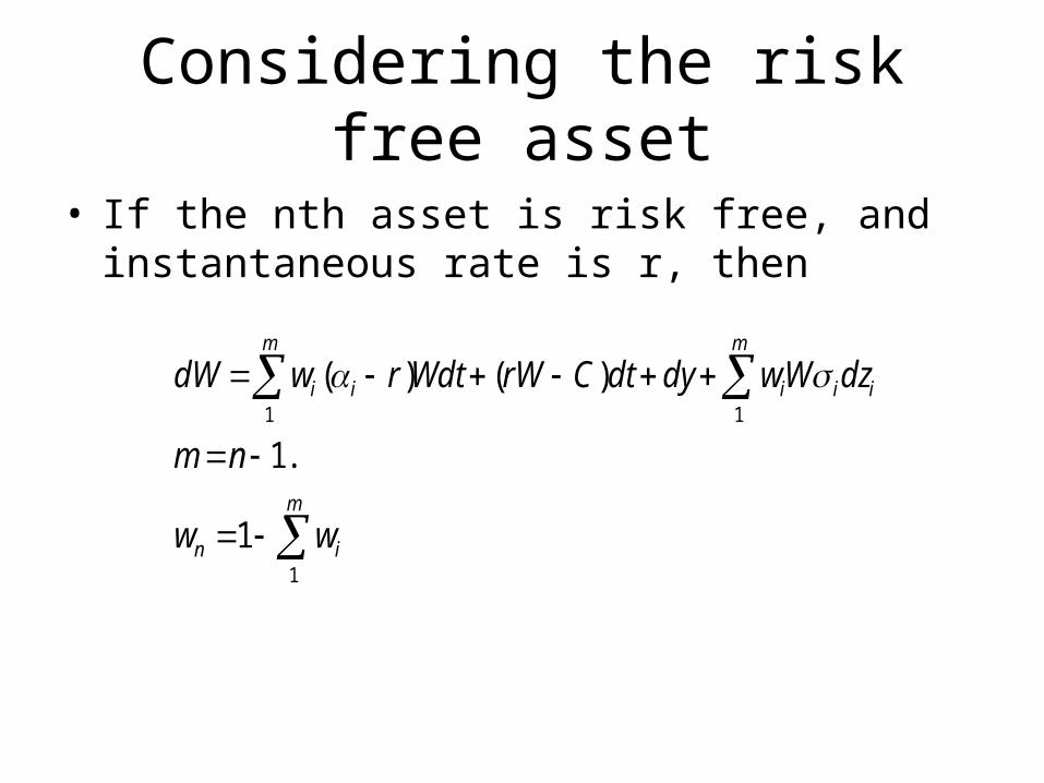
Considering the risk free asset
• If the nth asset is risk free, and instantaneous rate is r, then
m
in
m m
iiiii
ww
nm
dzWwdydtCrWWdtrwdW
1
1 1
1
.1
)()(

3.Optimal portfolio and consumption rules: the equations of optimality
• The problem of choosing the optimal portfolio and consumption rules,
• The dynamic programming equation is
• Then the partial differential equation becomes,
]}),([)),(({max00 TTWBdtttCUET
}]),([),({max),,(},{
T
ttwc
TTWBdssCUEtPWJ
n
iij
n
ji
n n
ijjij
n n
iij
n n
iiiii
PWWwP
PPP
WWww
PP
WCWw
ttCUtPWwC
1
2
1
1 12
2
2
22
1 1
1 1
2
1
2
1
2
1
)(),(),,;,(
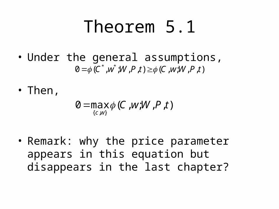
Theorem 5.1
• Under the general assumptions,
• Then,
• Remark: why the price parameter appears in this equation but disappears in the last chapter?
),,;,(),,;,(0 ** tPWwCtPWwC
),,;,(max0},{
tPWwCwc
Lagrangian solution
• Define the lagrangian
• Then first order conditions for maximum are
)1(1n
iwL
)3..(..............................10
)2........(,),(0
)1(..........,.........),(0
1
*
1 1
2***
**
n
i
n n
jkjjWjkjWWWkwk
WCC
wL
WPJWwJWJwCL
JUwCL
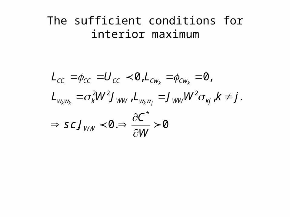
The sufficient conditions for interior maximum
0.0..
.,,
,0,0
*
222
W
CJcs
jkWJLJWL
LUL
WW
kjWWwwWWkww
CwCwCCCCCC
jkkk
kk
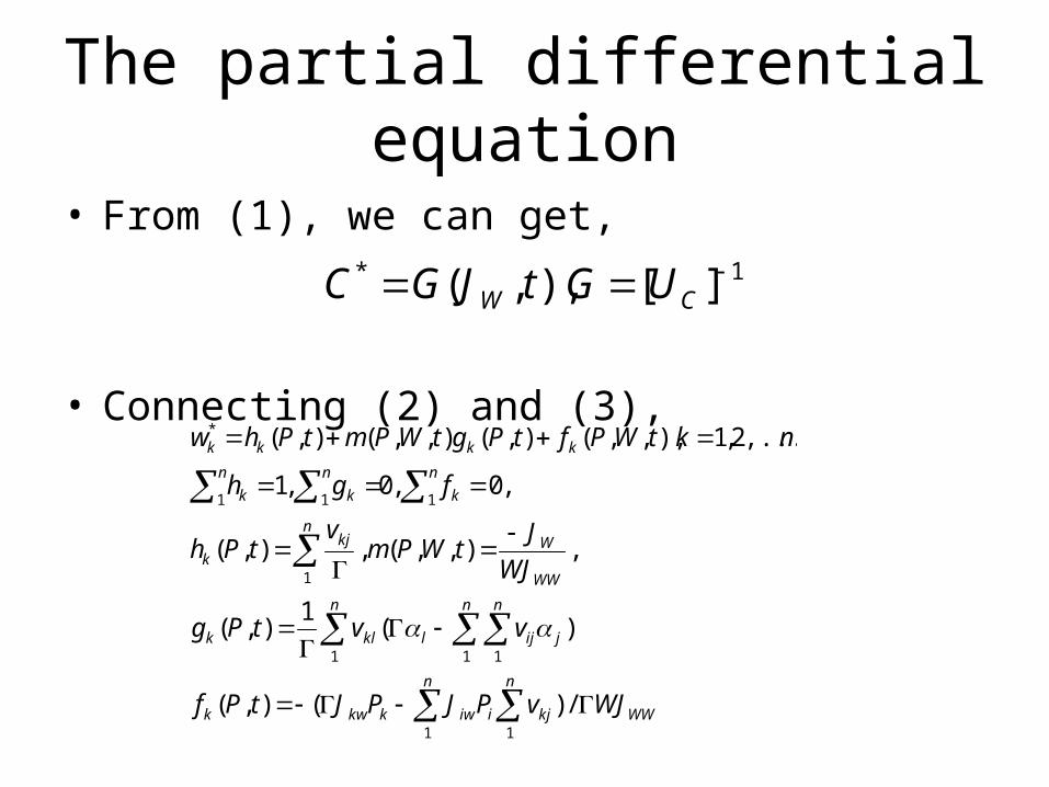
The partial differential equation
• From (1), we can get,
• Connecting (2) and (3),
1* ][),,( CW UGtJGC
n n
WWkjiiwkkwk
n n n
jijlklk
n
WW
Wkjk
n
k
n n
kk
kkkk
WJvPJPJtPf
vvtPg
WJ
JtWPm
vtPh
fgh
nktWPftPgtWPmtPhw
1 1
1 1 1
1
11 1
*
/)(),(
)(1
),(
,),,(,),(
,0,0,1
,...,2,1),,,(),(),,(),(
Partial differential equation(2)
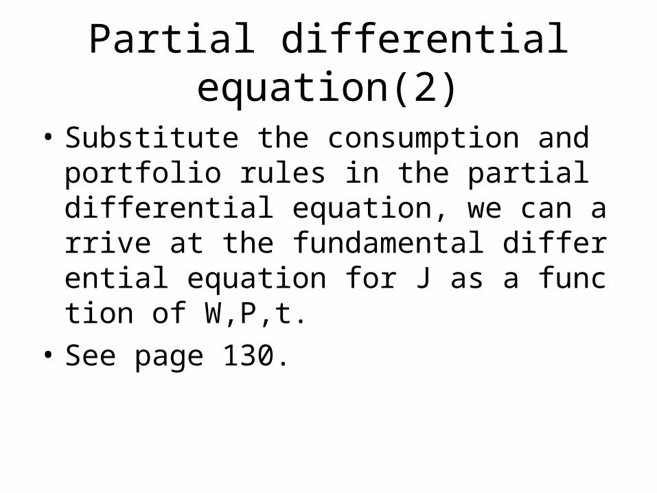
• Substitute the consumption and portfolio rules in the partial differential equation, we can arrive at the fundamental differential equation for J as a function of W,P,t.
• See page 130.
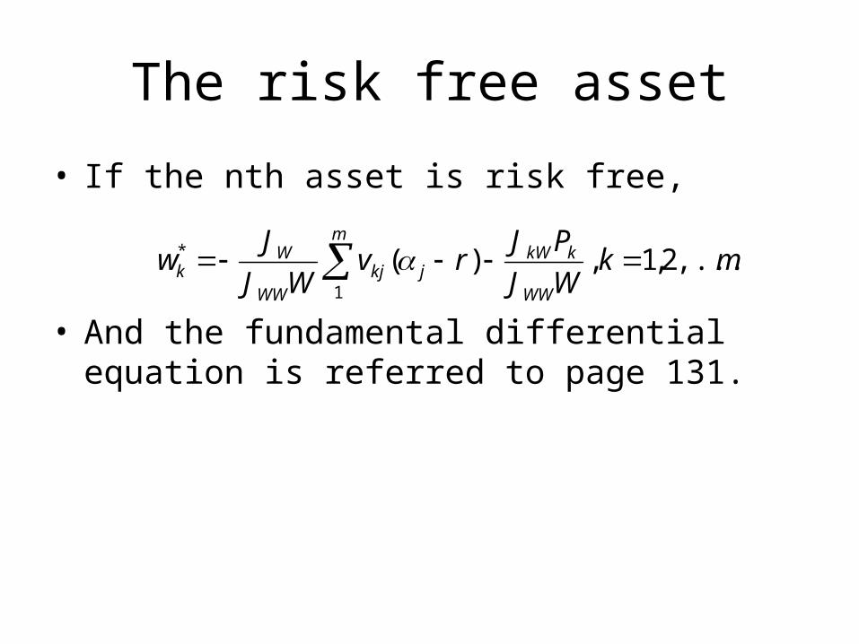
The risk free asset
• If the nth asset is risk free,
• And the fundamental differential equation is referred to page 131.
m
WW
kkWjkj
WW
Wk mk
WJ
PJrv
WJ
Jw
1
* ,...,2,1,)(
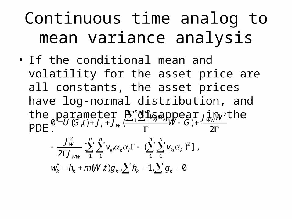
Continuous time analog to mean variance analysis
• If the conditional mean and volatility for the asset price are all constants, the asset prices have log-normal distribution, and the parameter P disappear in the PDE.
0,1,),(
],)([2
2)(),(0
*
1 1
2
1 1
2
21 1
kkkkk
n n n n
kkllkklWW
W
WW
n n
kkjWt
ghgtWmhw
vvJ
J
WJGW
vJJtGU

Theorem 5.2
• Separation or mutual fund theorem, individuals will be indifferent between choosing from a linear combination of these two funds or a linear combination of the original n assets.
• The price of fund is log-normally distributed.• The percentage of the mutual funds held in the kt
h asset are:
..,
,,1
constv
gv
hgv
h kkkkkk

Proof(1)
• Since• it is a parametric representation of a line in the hyperpla
ne defined by
• Then there exists two linearly independent vectors which form a basis for all optimal portfolios chosen by individuals.
• Each individual will be indifferent between choosing a linear combination of mutual fund shares or the combination of the original n assets.
kkk gtWmhw ),(*
n
kw1* 1
Proof(2)
normalP
const
dzudtu
V
dzPdtPN
V
dPNPdP
dPNdPN
dNdPdNPdPdNdNP
dPdNdNPdPNdNdPdNPdPNdV
PNPNV
f
kk
n n
kkkkk
n
kkkkkkffff
n
kkff
ffff
n n
kkkk
n n n
kkkkkkffffff
n
kkff
.log
.,
,
)(/
,
,
1 1
1
1
1 1
1 1 1
1

Proof(3)
• Let denote the proportion invested in the first fund.
• Then based on the mutual fund theorem,
• To solve these equations, we can suppose
•
);,( UtWa
nkaagtWmhw kkkkk ,...,2,1,)1(),(*
yx
yma
a
yamx
myaax
yghxgh kkkkk
,)1(
,)1(
,,

Simplified equation
• After some simple work, we can get
n n
kk
kkkkkk
tWvma
gv
hgv
h
1 11,1
),(
,,1

Corollary 5.2 risk free asset
• If the risk free asset is considered,
• Then use the same technique as theorem 5.2
m m m m
jkjknjkjk rvtWmwwrvtWmw1 1 1 1
*** )(),(11),(),(
m m
knkn
m
jkj
m
kjkjk rvv
rvv
1 1
11
1,1
)(),(1

Mean variance analysis
if we choose
Then one of the fund is risk free and the other fund is risky asset.
The mean-variance result is obtained.The log normal assumption in the continuous time
model is sufficient to allow the same analysis in mean variance model without the assumption of utility function or normality of absolute price changes.
m m
jij rvv1 1
)(,0

The risky asset
• In the present analysis, the risky asset can be always written by:
m m m
jijjkjk
m kkk
m m
kjjk
m
kk
rvrv
dzdz
dzdtPdP
1 1 1
1
1 1
2
1
),(/)(
/
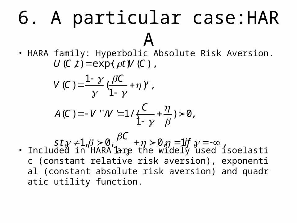
6. A particular case:HARA• HARA family: Hyperbolic Absolute Risk Aversion.
• Included in HARA are the widely used isoelastic (constant relative risk aversion), exponential (constant absolute risk aversion) and quadratic utility function.
,.1,01,0,1..
,0)1/(1'/'')(
,)1(
1)(
),()exp(),(
ifC
ts
CVVCA
CCV
CVttCU

The optimality problem
2*
)1/(1*
2
22)1/(
2
)(
)1()
)exp((
1)(
,2
)(]
)1([)
)exp()(exp(
)1(0
r
WJ
Jtw
JttC
r
J
JJrWJ
Jtt
WW
W
W
WW
WWt
W

solution
• See page 139.• Remark: the demand functions are linear in
wealth.• HARA family is the only class of concave utility
functions which imply linear solutions.• Definition: • HARA:• are at most function of time, and I is a
strictly concave function of X.
0)/(1/.),(),( XIIifXHARAtXI XXX
,
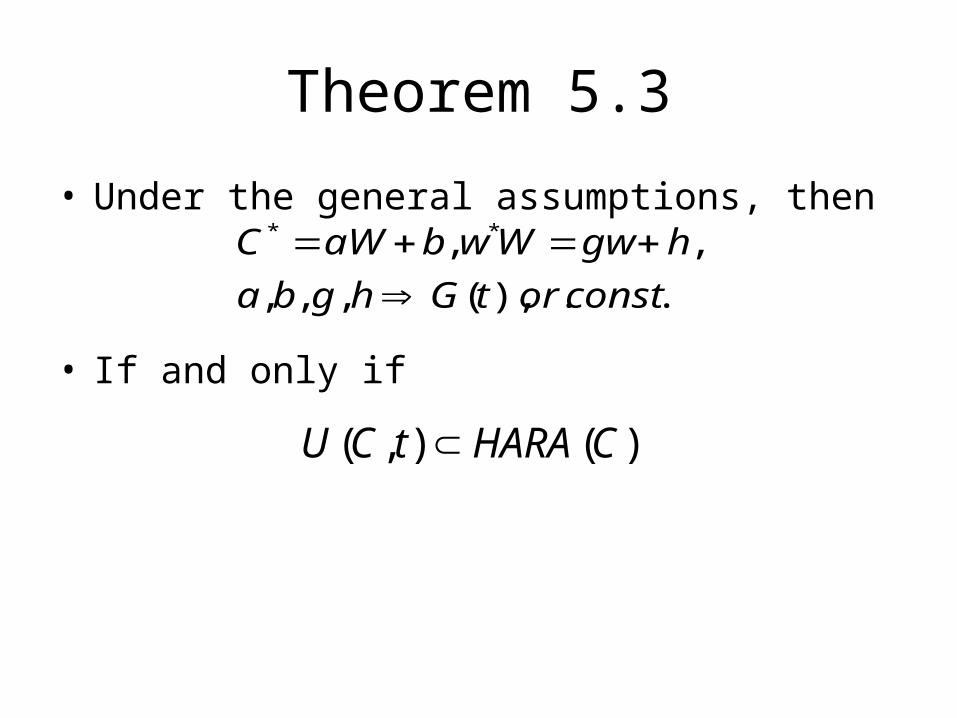
Theorem 5.3
• Under the general assumptions, then
• If and only if
..),(,,,
,, **
constortGhgba
hgwWwbaWC
)(),( CHARAtCU
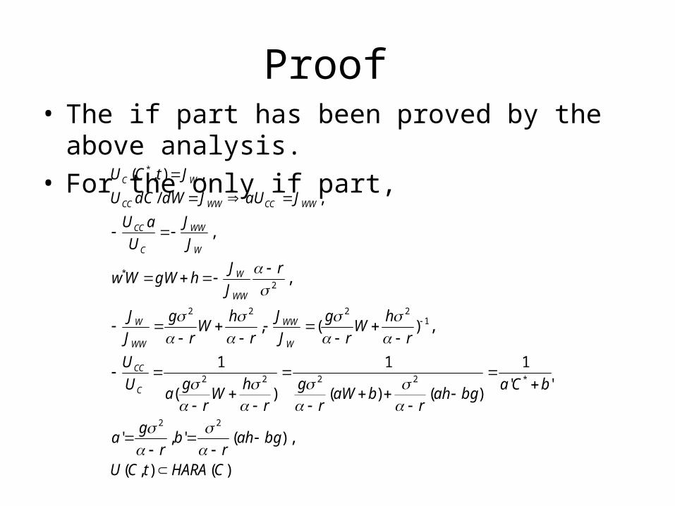
Proof • The if part has been proved by the above
analysis.• For the only if part,
)(),(
),(','
''
1
)()(
1
)(
1
,)(,
,
,
,/
,),(
22
*2222
12222
2*
*
CHARAtCU
bgahr
br
ga
bCabgah
rbaW
rg
rh
Wr
ga
U
U
r
hW
r
g
J
J
r
hW
r
g
J
J
r
J
JhgWWw
J
J
U
aU
JaUJdWdCU
JtCU
C
CC
W
WW
WW
W
WW
W
W
WW
C
CC
WWCCWWCC
WC

Theorem 5.4
• Given the model specified,
• If and only if
)(),( WHARAtWJ
)(CHARAU

Proof
• The if part has been proved by last theorem.• The only if part:• If • Then based on
• w*W is linear function of wealth.
)(),( WHARAtWJ
2* )(
r
WJ
Jtw
WW
W
Proof(2)
• Based on:
• Differentiating this with respect to wealth,
• This is linear in wealth if J is HARA.
222
},{ 2
1]))([()((max0 WwJCWrrwJJCU WWWt
wC
2
22
2
2
2
22
2
2
2
)()(
)(
,2
)()(
)(0
r
J
J
J
Jr
J
J
J
Jr
J
JrWC
r
J
JJ
rJCJrWJrJJ
WW
W
WW
WWW
WW
W
WW
W
WW
tW
WW
WWWWWWWWWWtW
The stochastic process of the wealth
• See page 141.

Theorem 5.5
• Is log normal if and only if
),()( * tCUtY
)(),( CHARAtCU

proof
• The if part has been proved.
• For the only if part, suppose
• Then,
),(),,( ** tWfWwtWgC
,)(
,)2/1)((
,))((
,)(2/1
,)(2/1
22*
2*
2**
dzfgUdtYmdY
dzfgdtgfgggrWgrfgdC
fdzdtgrWrfdW
dWgdtgdWgdC
dCUdtUdCUdY
WC
WtWWWWW
WWtW
CCtC

Proof(2)
• If Y is log-normal,
)1/(1
2
2
)]())(1[(
,)()(
,)(/
,,
,/
tuCU
U
Ut
U
U
tb
r
U
U
U
UrfgUbU
r
J
JfJgU
UUfgb
CC
C
CC
CC
CWC
WW
WWWWCC
CW
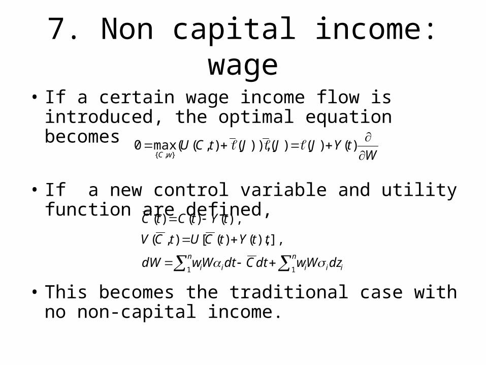
7. Non capital income: wage
• If a certain wage income flow is introduced, the optimal equation becomes
• If a new control variable and utility function are defined,
• This becomes the traditional case with no non-capital income.
WtYJJJtCU
wC
)()()()),(),((max0},{
n n
iiiii dzWwdtCdtWwdW
ttYtCUtCV
tYtCtC
1 1
],),()([),(
),()()(
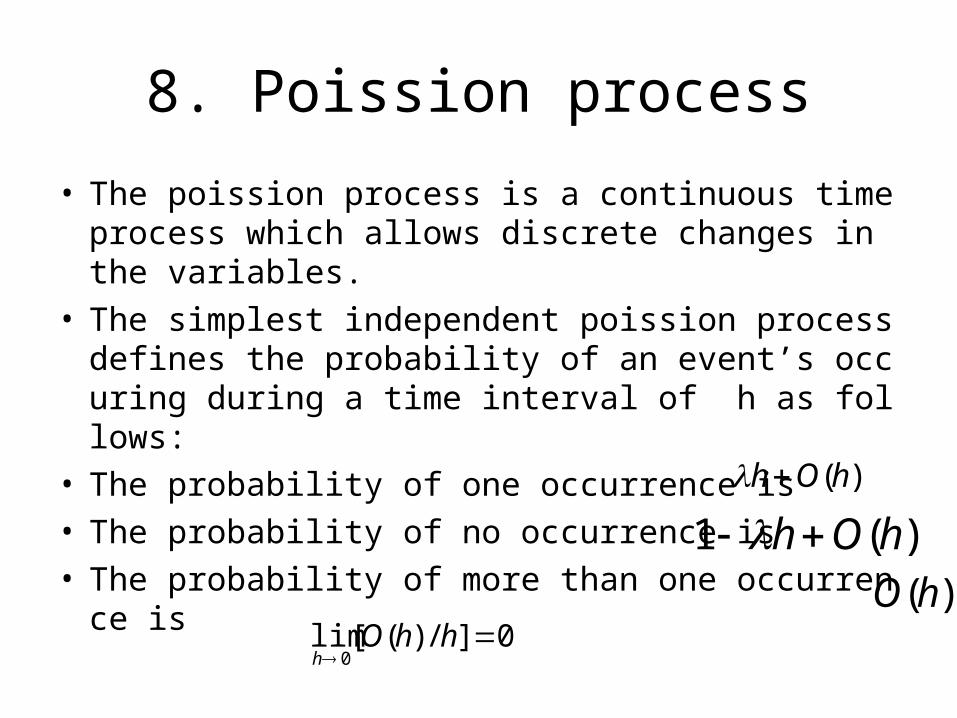
8. Poission process
• The poission process is a continuous time process which allows discrete changes in the variables.
• The simplest independent poission process defines the probability of an event’s occuring during a time interval of h as follows:
• The probability of one occurrence is • The probability of no occurrence is • The probability of more than one occurrence is
)(hOh
)(1 hOh )(hO
0]/)([lim0
hhOh
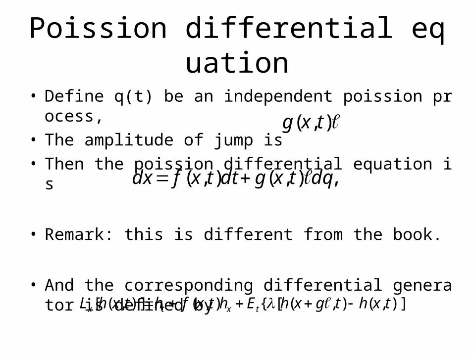
Poission differential equation
• Define q(t) be an independent poission process,• The amplitude of jump is • Then the poission differential equation is
• Remark: this is different from the book.
• And the corresponding differential generator is defined by
),( txg
,),(),( dqtxgdttxfdx
)]},(),([{),()],([ txhtgxhEhtxfhtxhL txtx
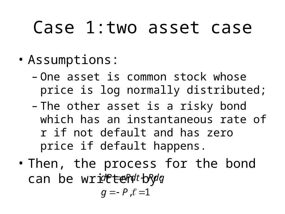
Case 1:two asset case
• Assumptions:– One asset is common stock whose price is log
normally distributed;– The other asset is a risky bond which has an
instantaneous rate of r if not default and has zero price if default happens.
• Then, the process for the bond can be written by:
1,
Pg
PdqrPdtdP
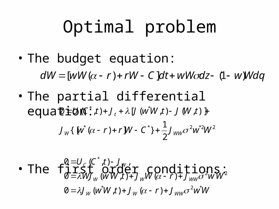
Optimal problem
• The budget equation:
• The partial differential equation:
• The first order conditions:
WdqwdzwWdtCrWrwWdW )1(])([
22*2**
**
2
1}])({[
)],(),([),(0
WwJCWrrwJ
tWJtWwJJtCU
WWW
t
WwJrJtWwJ
WwJrWJtWwWJ
JtCU
WWWW
WWWW
WC
*2*
2*2*
*
)(),(0
)(),(0
,),(0
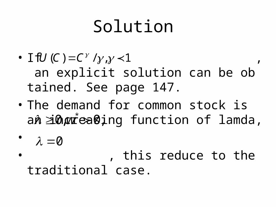
Solution
• If , an explicit solution can be obtained. See page 147.
• The demand for common stock is an increasing function of lamda,
•
• , this reduce to the traditional case.
1,/)( CCU
,0,0 * w0

Case 2: if wage increase is poission
• The wage is incremented by a constant amount at random time,
• For two asset case,
1, dqdY
),,()exp(),(
2/1
}])({[
)],(),([),()(0
)()exp(),(
22*2
**
*
tYWItYWJ
WwJ
CYWrrwJ
YWJYWJYWJCV
CVttCU
WW
W

The optimal consumption and portfolio rules
• If
• Then the optimal consumption and portfolio rules are:
•
/)exp()( CCV
r
rtWtw
rr
rrr
tYtWrtC
2*
2
2
2*
)()(
]2
)([
1])exp(1)(
)([)(

Implication • For consumption,• is the present value of wealth and
constant wage.• is the present value of future
wage increment.• It is discounted by larger rate than the risk free
rate reflecting the investor’s risk aversion since,
rtYtW /)()(
)exp(1
2
r
0.,)]exp(1[
)())(exp(
))()())((exp(
2
2
ifr
rdststsr
sdtYsYtsrE
t
tt

Implication(2)• The individual, in computing the present value of future
wage increment, determines the certainty equivalent flow and then discount it at risk free rate.
• Proof: (remark: but in fact, it is a approximation)
2
0 00
0
00
0
)]exp(1[)0(
)exp())exp(1(
)exp()0()()exp(
,/)]exp(1[)0()(
)]exp()0((exp[1
)exp()exp(!
)())0(exp(
1))((exp(
1)}(exp{
)]([)]([
rr
Y
dsrssdsrsYsXrs
tYtX
ttYE
ktk
tYtYE
tX
tYUEtXU
k
k

Case 3: event of death is poission
• The age of death is the first time that event of death occurs. Then the optimal criterion is
•
• The correspondent optimality equation:
}]),([),({max00
WBdttCUE
)()],(),([),(0 * JLtWJtWBtCU
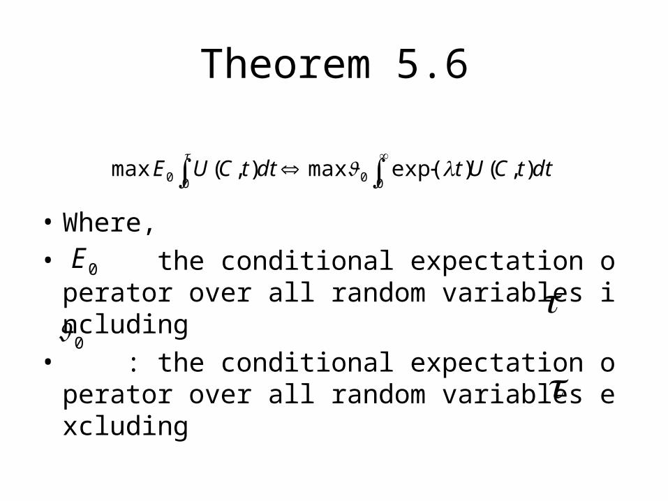
Theorem 5.6
• Where,
• the conditional expectation operator over all random variables including
• : the conditional expectation operator over all random variables excluding
0000 ),()exp(max),(max dttCUtdttCUE
0E
0
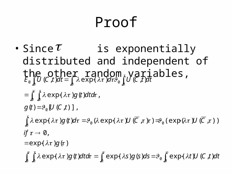
Proof
• Since is exponentially distributed and independent of the other random variables,
0 0 0 00
00 0
0
0 0
0 0 000
),()exp()()exp()()exp(
)()exp(
,0.
)),,()(exp()),()exp(()()exp(
)],,([)(
,)()exp(
),()exp(),(
dttCUtdssgsdtdtg
g
if
CUCUdtg
tCUtg
dtdtg
dttCUddttCUE

Implication
• The individual acts as he will live forever, but with a subjective rate of force of mortality, i.e., the reciprocal of his life expectancy.
9. Alternative price expectations
• Three types of alternative price mechanisms are analyzed here:– Asymptotic normal price level hypothesis;– The instantaneous rate of return is stochastic in
geometric Brownian Motion;– It is assumed that the investor does not know
the true value of expected return, but must estimate it.

Case 1
• It is assumed that there exists a normal price function such that,
• The investor expects the long run price to approach the normal price.
• one example:
)(tP
tTtPtPETt
0,1))(/)((lim
2/)),0(/)(log(
,)(
)),0(/)0(log(,4//
,))}0(/)(log({
),exp()0()(
2
2
uPtPY
dzdtYvtudY
PPkvk
dzdtPtPvtP
dP
vtPtP
Implication
• The price adjustment is exponentially regressive toward the normal price;
• The log return is normally distributed variable generated by Markov process and does not have independent increments.
• The price is log normal and Markov.
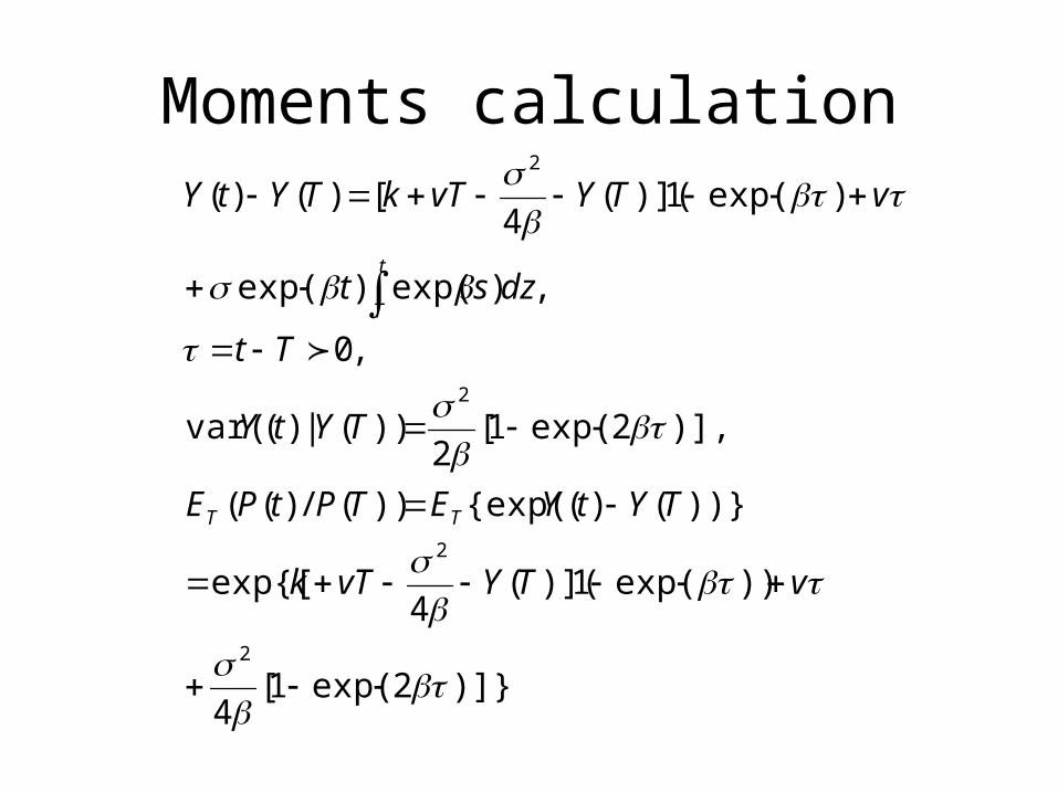
Moments calculation
)]}2exp(1[4
))exp(1)]((4
exp{[
))}()({exp())(/)((
)],2exp(1[2
))(|)(var(
,0
,)exp()exp(
)exp(1)]((4
[)()(
2
2
2
2
vTYvTk
TYtYETPtPE
TYtY
Tt
dzst
vTYvTkTYtY
TT
t
T
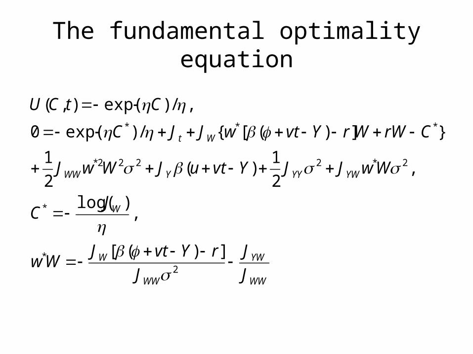
The fundamental optimality equation
WW
YW
WW
W
W
YWYYYWW
Wt
J
J
J
rYvtJWw
JC
WwJJYvtuJWwJ
CrWWrYvtwJJC
CtCU
2*
*
2*2222*
***
])([
,)log(
,2
1)(
2
1
}])([{/)exp(0
,/)exp(),(
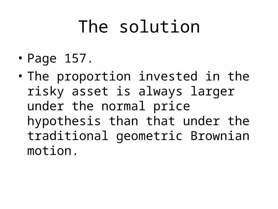
The solution
• Page 157.
• The proportion invested in the risky asset is always larger under the normal price hypothesis than that under the traditional geometric Brownian motion.

Case 2
• Remark: it was first introduced by Frank De Leeuw to explain the interest rate behavior.
dzdtud
dzdtdP
)(
,

The portfolio rules
• In similar way, we can get the optimal portfolio rules for the investor.
• Note that under the traditional assumption (expected return of risky asset is larger than risk free rate), the investor will hold less proportion of wealth in risky asset than under the geometric Brownian motion.
• The amount invested in risky asset is decreasing function of u. as u increases, the probability of future be more favorable than current, thus investor will save more as reserve for future investment.
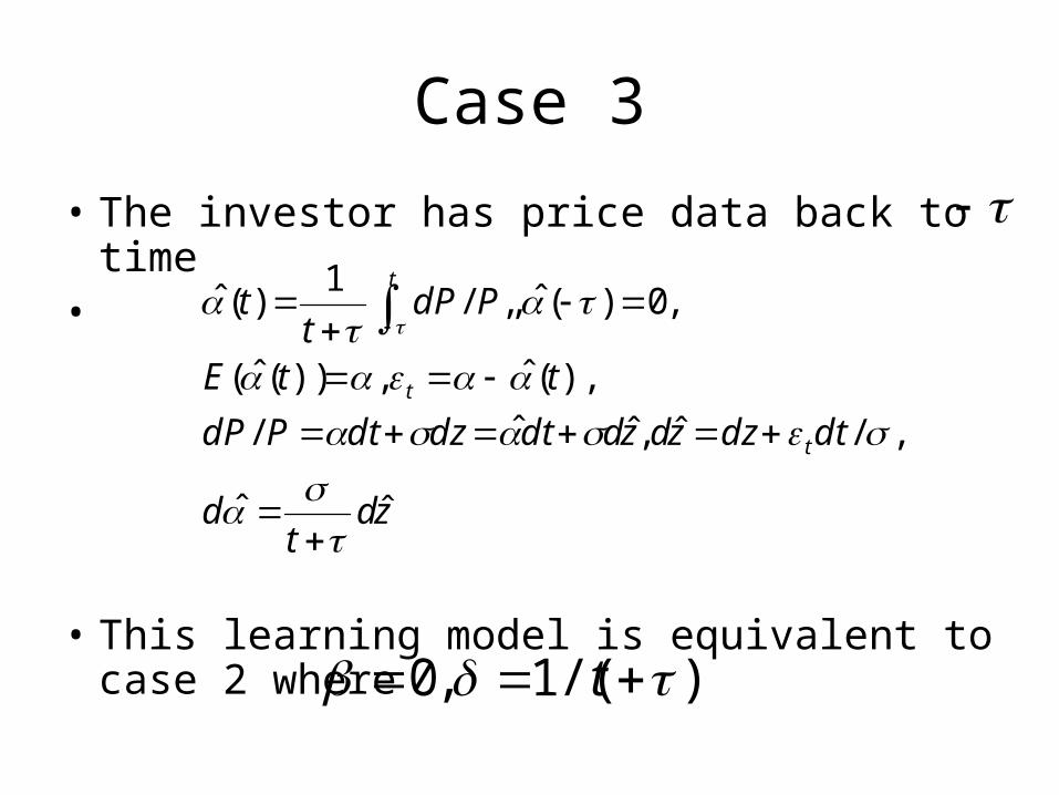
Case 3
• The investor has price data back to time•
• This learning model is equivalent to case 2 where
zdt
d
dtdzzdzddtdzdtPdP
ttE
PdPt
t
t
t
t
ˆˆ
,/ˆ,ˆˆ/
),(ˆ,))(ˆ(
,0)(ˆ,,/1
)(ˆ
)/(1,0 t
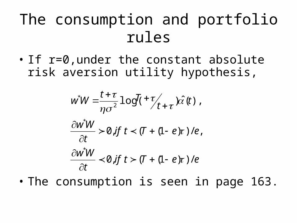
The consumption and portfolio rules
• If r=0,under the constant absolute risk aversion utility hypothesis,
• The consumption is seen in page 163.
eeTtift
Ww
eeTtift
Ww
ttTt
Ww
/))1((.,0
,/))1((.,0
),(ˆ)log(
*
*
2*

Implication
• In early life, the investor learns more about the price equation with each observation, hence investment in the risky asset becomes more attractive.
• But as he approaches the end of life, he is generally liquidating his portfolio to consume a larger fraction of wealth.
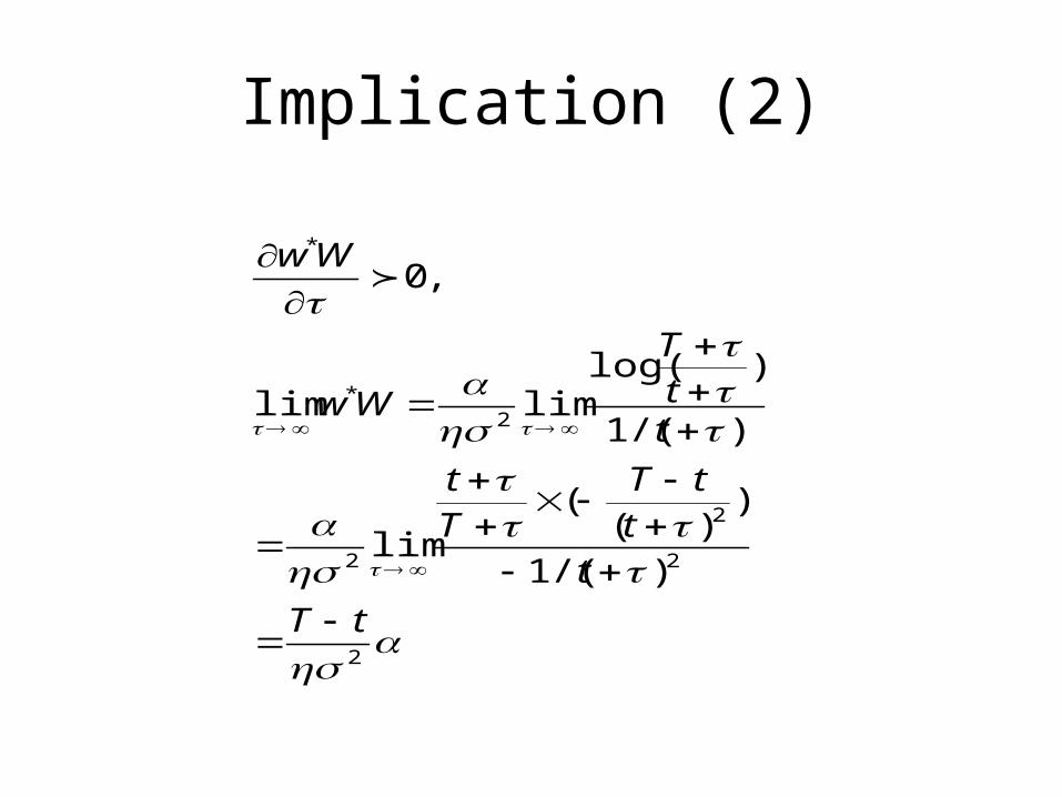
Implication (2)
2
2
2
2
2*
*
)/(1
))(
(lim
)/(1
)log(limlim
,0
tT
tt
tTTt
ttT
Ww
Ww
10. conclusions
• By dynamic programming method, the way to systematically construct and analyze optimal continuous time dynamic models under uncertainty is shown and is applicable to a wide class of economic models.
• In continuous time, one important advantage is that it only consider two types of stochastic process.
• This model is expended by considering the assumption of HARA family utility function, introduction of stochastic wage, risk of default, uncertainty about life expectancy, and alternative types of price dynamics.

Thanks!