CFD in COMSOL Multiphysics
Mats Nigam
© Copyright 2016 COMSOL. Any of the images, text, and equations here may be copied and modified for your own internal use. All trademarks are the property of their respective owners. See www.comsol.com/trademarks.

Worldwide Sales Offices
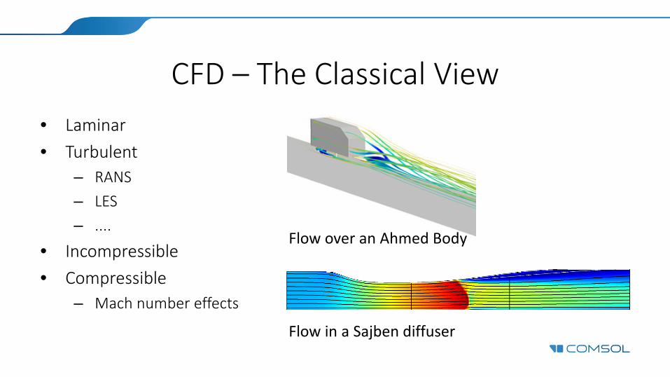
CFD – The Classical View • Laminar • Turbulent
– RANS – LES – ....
• Incompressible • Compressible
– Mach number effects
Flow over an Ahmed Body
Flow in a Sajben diffuser
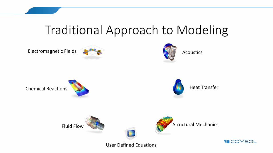
Traditional Approach to Modeling
Fluid Flow
Chemical Reactions
Acoustics Electromagnetic Fields
Heat Transfer
Structural Mechanics
User Defined Equations
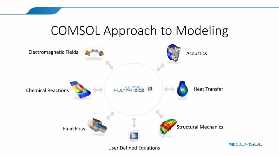
COMSOL Approach to Modeling
Fluid Flow
Chemical Reactions
Acoustics Electromagnetic Fields
Heat Transfer
Structural Mechanics
User Defined Equations
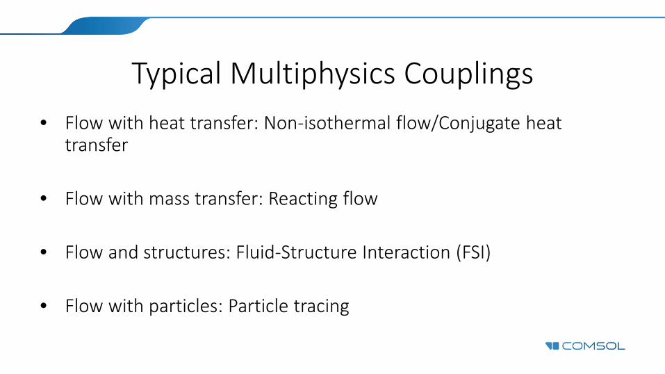
Typical Multiphysics Couplings • Flow with heat transfer: Non-isothermal flow/Conjugate heat
transfer • Flow with mass transfer: Reacting flow • Flow and structures: Fluid-Structure Interaction (FSI) • Flow with particles: Particle tracing
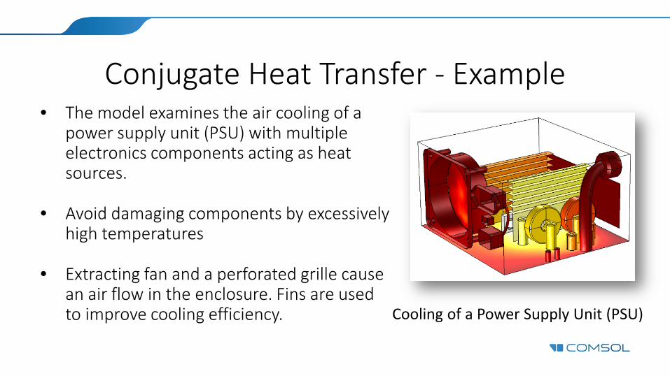
Conjugate Heat Transfer - Example • The model examines the air cooling of a
power supply unit (PSU) with multiple electronics components acting as heat sources.
• Avoid damaging components by excessively high temperatures
• Extracting fan and a perforated grille cause an air flow in the enclosure. Fins are used to improve cooling efficiency.
Cooling of a Power Supply Unit (PSU)
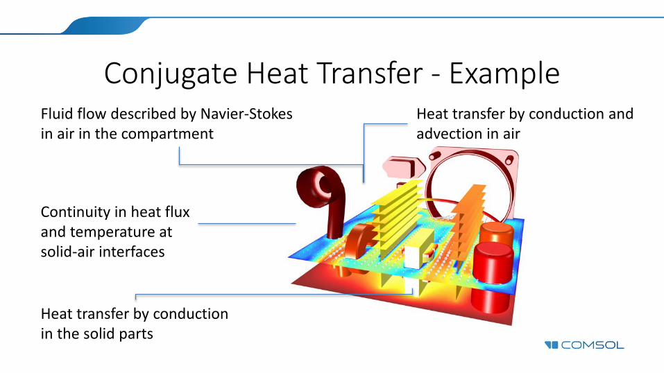
Conjugate Heat Transfer - Example Fluid flow described by Navier-Stokes in air in the compartment
Heat transfer by conduction in the solid parts
Heat transfer by conduction and advection in air
Continuity in heat flux and temperature at solid-air interfaces
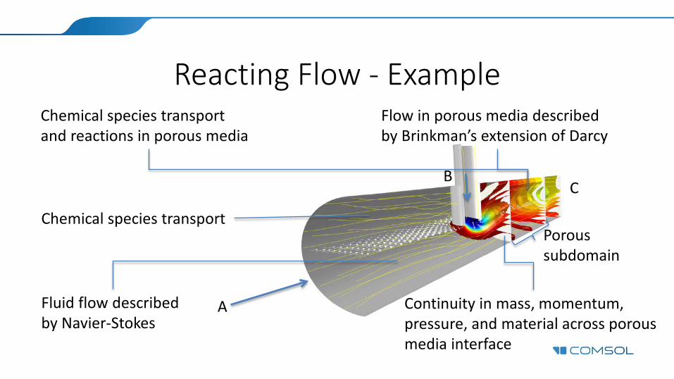
Reacting Flow - Example Chemical species transport and reactions in porous media
Chemical species transport
Flow in porous media described by Brinkman’s extension of Darcy
Continuity in mass, momentum, pressure, and material across porous media interface
Fluid flow described by Navier-Stokes
Porous subdomain
A
B C

Fluid-Structure Interaction - Example Liquid phase described by Navier-Stokes
Solid mechanics in the obstacle with moving mesh
Gas phase described by Navier-Stokes
Interface between the two fluids modeled with phase fields
Interface between solid and fluid described by moving mesh using the ALE method
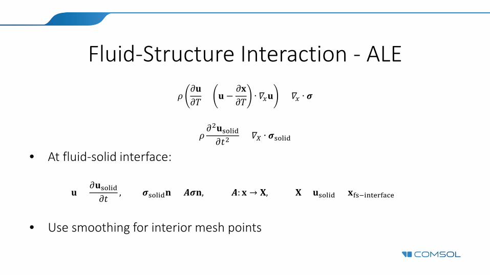
Fluid-Structure Interaction - ALE
𝜌𝜕𝐮𝜕𝜕 + 𝐮 −
𝜕𝐱𝜕𝜕 ∙ 𝛻𝑥𝐮 = 𝛻𝑥 ∙ 𝝈
𝜌𝜕2𝐮solid𝜕𝑡2 = 𝛻𝑋 ∙ 𝝈solid
• At fluid-solid interface:
𝐮 =𝜕𝐮solid𝜕𝑡 , 𝝈solid𝐧 = 𝑨𝝈𝐧, 𝑨: 𝐱 → 𝐗, 𝐗 + 𝐮solid = 𝐱fs−interface
• Use smoothing for interior mesh points
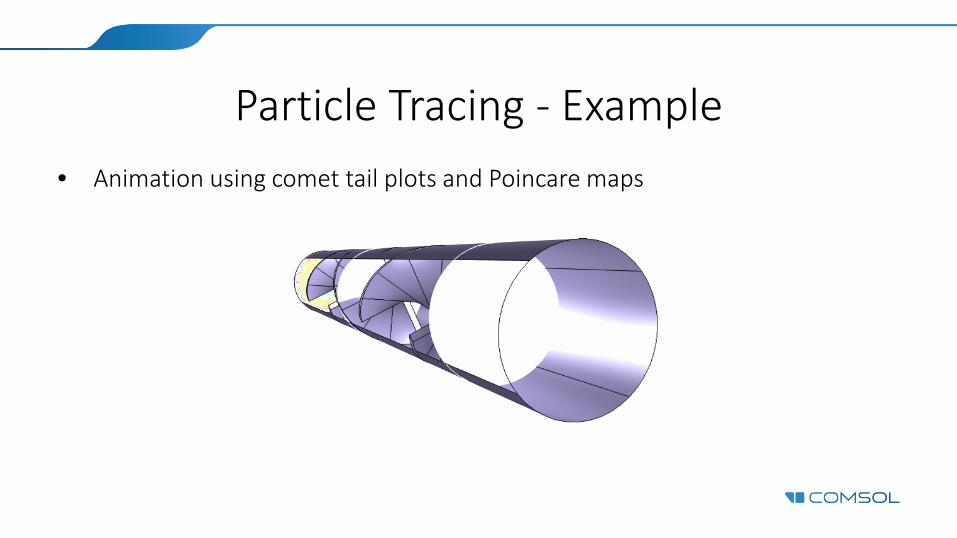
Particle Tracing - Example • Animation using comet tail plots and Poincare maps
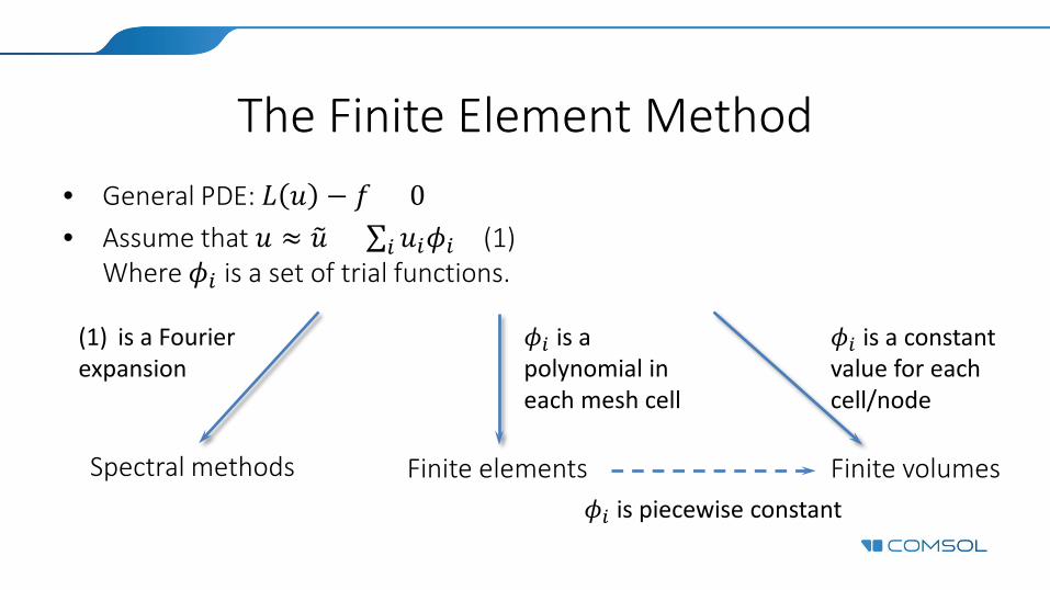
The Finite Element Method • General PDE: 𝐿 𝑢 − 𝑓 = 0 • Assume that 𝑢 ≈ 𝑢� = ∑ 𝑢𝑖𝜙𝑖𝑖 (1)
Where 𝜙𝑖 is a set of trial functions.
(1) is a Fourier expansion
Spectral methods
𝜙𝑖 is a polynomial in each mesh cell
Finite elements
𝜙𝑖 is a constant value for each cell/node
Finite volumes 𝜙𝑖 is piecewise constant
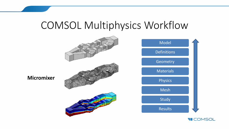
COMSOL Multiphysics Workflow
Micromixer
Model
Definitions
Geometry
Materials
Physics
Mesh
Study
Results
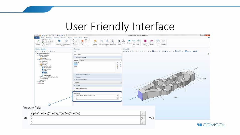
User Friendly Interface

Everything is Equation Based
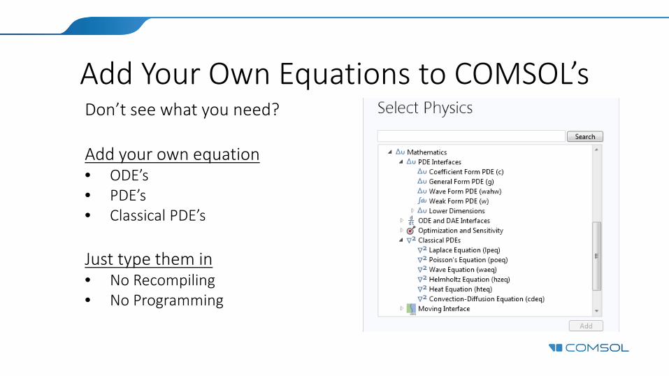
Add Your Own Equations to COMSOL’s Don’t see what you need? Add your own equation • ODE’s • PDE’s • Classical PDE’s
Just type them in • No Recompiling • No Programming
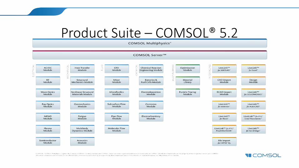
Product Suite – COMSOL® 5.2
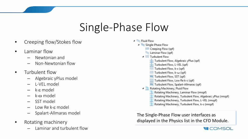
Single-Phase Flow • Creeping flow/Stokes flow
• Laminar flow – Newtonian and – Non-Newtonian flow
• Turbulent flow – Algebraic yPlus model – L-VEL model – k-ε model – k-ω model – SST model – Low Re k-ε model – Spalart-Allmaras model
• Rotating machinery – Laminar and turbulent flow
The Single-Phase Flow user interfaces as displayed in the Physics list in the CFD Module.

Single-Phase Flow General functionality for both laminar and turbulent flow
• Swirl flow
– Includes the out-of-plane velocity component for axisymmetric flows
• Specific boundary conditions
– Fully developed laminar inflow and outflow for simulating long inlet and outlet channels
– Assembly boundaries for geometries consisting of several parts
– Wall conditions on internal shells for simulating thin immersed structures
– Screen conditions for simulating thin perforated plates and wire gauzes
Streamlines in an HVAC duct

Turbulent Flow with Wall Functions • Models with wall functions
– k-ε model • The standard k-ε model with realizability constraints • The basic industrial modeling tool
– k-ω model • The revised Wilcox k-ω model (1998) with realizability
constraints
• Versatile and easy to use models
• Wall functions for smooth and rough walls
Flow in a pipe elbow simulated with the k-ω model.

Wall Resolved Turbulent Flow • Algebraic turbulence models
– Algebraic yPlus model – L-VEL model
Turbulent viscosity is defined from local flow speed and wall distance – no additional boundary conditions
• Transport-equation models
– SST model with realizability constraints – Low Re k-ε turbulence model with realizability constraints – Spalart-Allmaras model with rotational correction
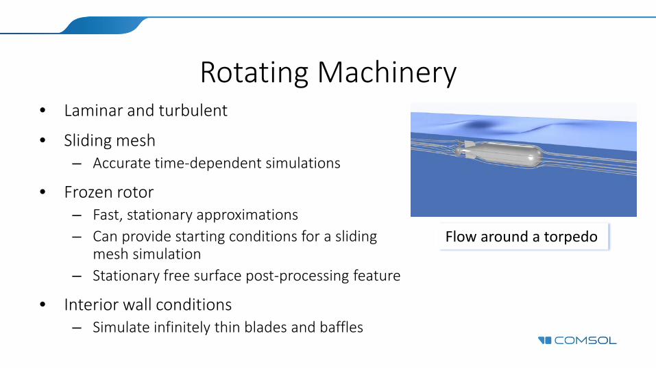
Rotating Machinery • Laminar and turbulent
• Sliding mesh – Accurate time-dependent simulations
• Frozen rotor – Fast, stationary approximations – Can provide starting conditions for a sliding
mesh simulation – Stationary free surface post-processing feature
• Interior wall conditions – Simulate infinitely thin blades and baffles
Flow around a torpedo
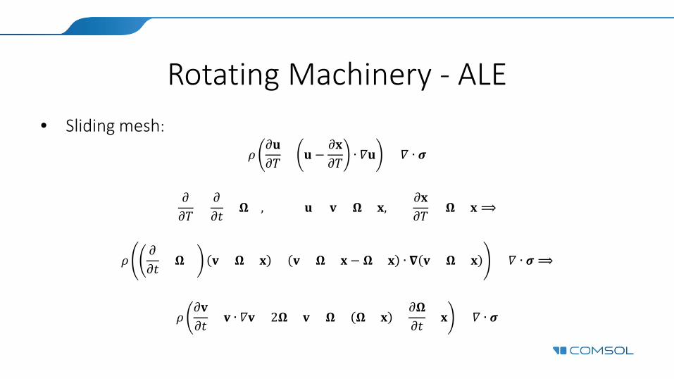
Rotating Machinery - ALE • Sliding mesh:
𝜌𝜕𝐮𝜕𝜕 + 𝐮 −
𝜕𝐱𝜕𝜕 ∙ 𝛻𝐮 = 𝛻 ∙ 𝝈
𝜕𝜕𝜕 =
𝜕𝜕𝑡 + 𝛀 ×, 𝐮 = 𝐯 + 𝛀 × 𝐱,
𝜕𝐱𝜕𝜕 = 𝛀 × 𝐱 ⟹
𝜌𝜕𝜕𝑡 + 𝛀 × 𝐯 + 𝛀 × 𝐱 + 𝐯 + 𝛀 × 𝐱 − 𝛀 × 𝐱 ∙ 𝛁 𝐯 + 𝛀 × 𝐱 = 𝛻 ∙ 𝝈 ⟹
𝜌𝜕𝐯𝜕𝑡 + 𝐯 ∙ 𝛻𝐯 + 2𝛀 × 𝐯 + 𝛀 × 𝛀 × 𝐱 +
𝜕𝛀𝜕𝑡 × 𝐱 = 𝛻 ∙ 𝝈
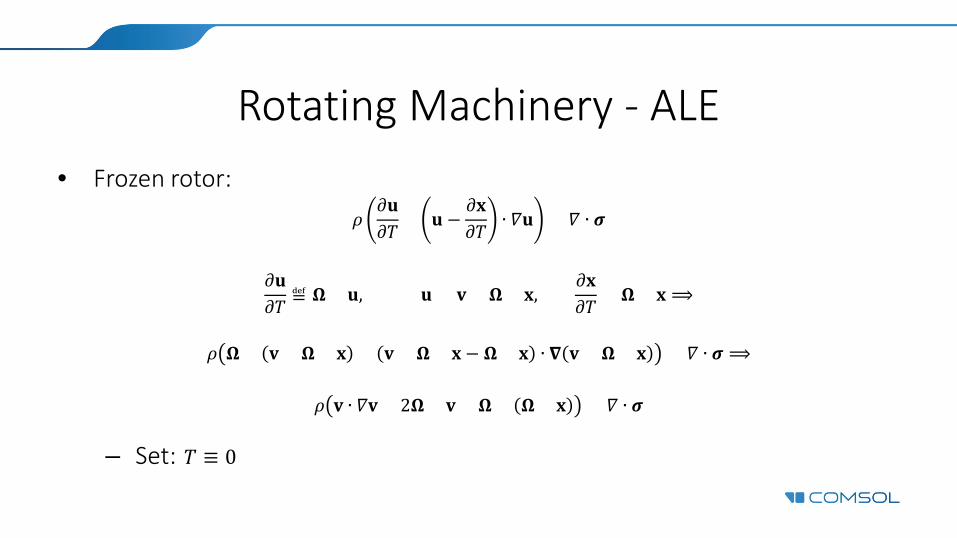
Rotating Machinery - ALE • Frozen rotor:
𝜌𝜕𝐮𝜕𝜕 + 𝐮 −
𝜕𝐱𝜕𝜕 ∙ 𝛻𝐮 = 𝛻 ∙ 𝝈
𝜕𝐮𝜕𝜕 ≝ 𝛀 × 𝐮, 𝐮 = 𝐯 + 𝛀 × 𝐱,
𝜕𝐱𝜕𝜕 = 𝛀 × 𝐱 ⟹
𝜌 𝛀 × 𝐯 + 𝛀 × 𝐱 + 𝐯 + 𝛀 × 𝐱 − 𝛀 × 𝐱 ∙ 𝛁 𝐯 + 𝛀 × 𝐱 = 𝛻 ∙ 𝝈 ⟹
𝜌 𝐯 ∙ 𝛻𝐯 + 2𝛀 × 𝐯 + 𝛀 × 𝛀 × 𝐱 = 𝛻 ∙ 𝝈
– Set: 𝜕 ≡ 0
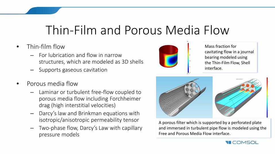
Thin-Film and Porous Media Flow • Thin-film flow
– For lubrication and flow in narrow structures, which are modeled as 3D shells
– Supports gaseous cavitation
• Porous media flow – Laminar or turbulent free-flow coupled to
porous media flow including Forchheimer drag (high interstitial velocities)
– Darcy’s law and Brinkman equations with isotropic/anisotropic permeability tensor
– Two-phase flow, Darcy’s Law with capillary pressure models
A porous filter which is supported by a perforated plate and immersed in turbulent pipe flow is modeled using the Free and Porous Media Flow interface.
Mass fraction for cavitating flow in a journal bearing modeled using the Thin-Film Flow, Shell interface.
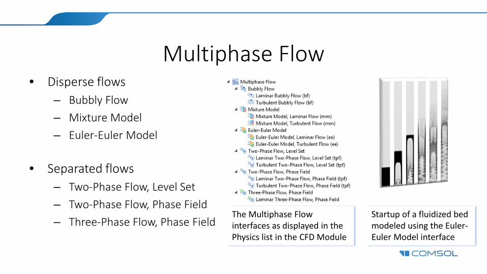
Multiphase Flow • Disperse flows
– Bubbly Flow – Mixture Model – Euler-Euler Model
• Separated flows – Two-Phase Flow, Level Set – Two-Phase Flow, Phase Field – Three-Phase Flow, Phase Field
The Multiphase Flow interfaces as displayed in the Physics list in the CFD Module
Startup of a fluidized bed modeled using the Euler-Euler Model interface

Multiphase Flow – Disperse Flows The equations of motion are averaged over volumes which are small compared to the computational domain but large compared to the size of the dispersed particles/bubbles/droplets.
• Bubbly Flow & Mixture Model – Closures for the relative motion (slip) between the two phases assume that the particle relaxation time is
small compared to the time scale of the mean flow. – For Bubbly flow, bubble concentration must be small (~0.1) unless coalescence is explicitly accounted for – Bubble induced turbulence in bubbly flow – Mass transfer between phases – Option to solve for interfacial area – Spherical and non-spherical particles
• Euler-Euler Flow – General two-phase flow – No restriction on particle relaxation time – Spherical and non-spherical particles – Mixture or phase-specific turbulence model Bubble-induced turbulent flow in an airlift loop reactor
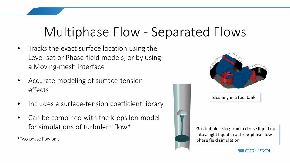
Multiphase Flow - Separated Flows • Tracks the exact surface location using the
Level-set or Phase-field models, or by using a Moving-mesh interface
• Accurate modeling of surface-tension effects
• Includes a surface-tension coefficient library
• Can be combined with the k-epsilon model for simulations of turbulent flow* Gas bubble rising from a dense liquid up
into a light liquid in a three-phase flow, phase field simulation *Two-phase flow only
Sloshing in a fuel tank
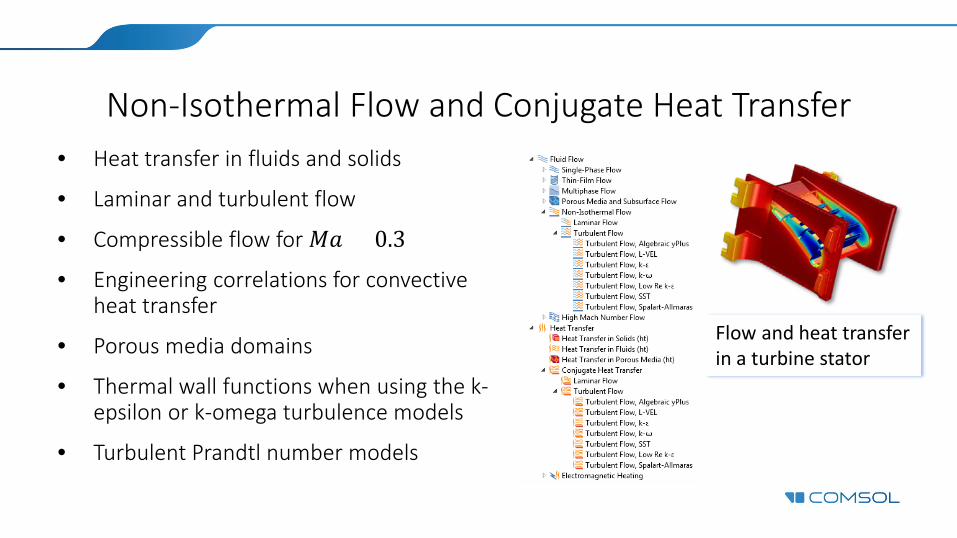
Non-Isothermal Flow and Conjugate Heat Transfer • Heat transfer in fluids and solids
• Laminar and turbulent flow
• Compressible flow for 𝑀𝑀 < 0.3
• Engineering correlations for convective heat transfer
• Porous media domains
• Thermal wall functions when using the k-epsilon or k-omega turbulence models
• Turbulent Prandtl number models
Flow and heat transfer in a turbine stator

High Mach Number Flow • Laminar and turbulent flow
• k-ε turbulence model
• Spalart-Allmaras model
• Fully compressible flow for all Mach numbers
• Viscosity and conductivity can be determined from Sutherland’s law
Turbulent compressible flow in a two-dimensional Sajben diffuser
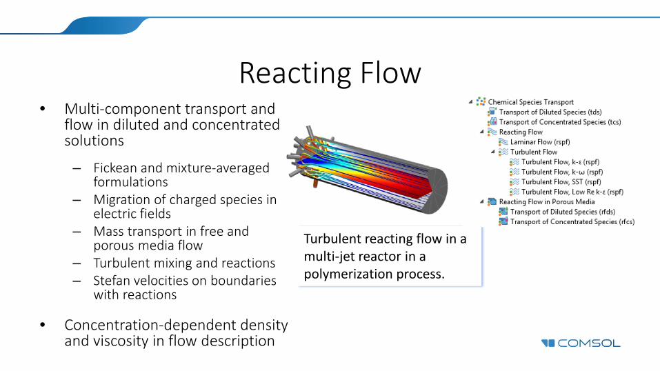
Reacting Flow • Multi-component transport and
flow in diluted and concentrated solutions
– Fickean and mixture-averaged formulations
– Migration of charged species in electric fields
– Mass transport in free and porous media flow
– Turbulent mixing and reactions – Stefan velocities on boundaries
with reactions
• Concentration-dependent density and viscosity in flow description
Turbulent reacting flow in a multi-jet reactor in a polymerization process.

From Model to App • Simulations today:
– Mostly used by dedicated simulation engineers and scientists – just like you!
– Require some degree of training to get started
• Simulations tomorrow:
R&D
Engineering
Manufacturing
Installation
Sales
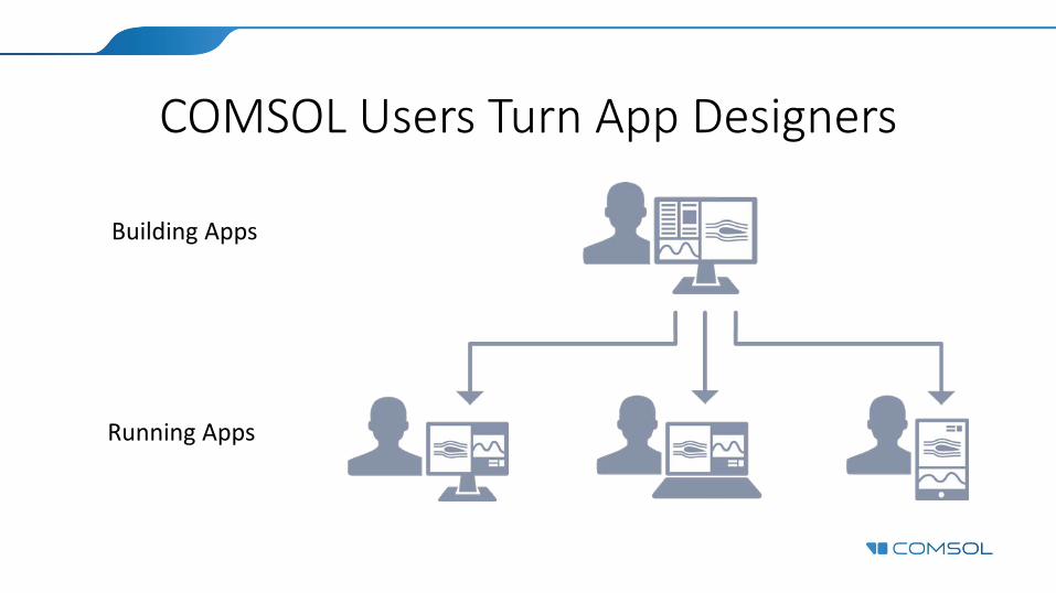
COMSOL Users Turn App Designers
Building Apps
Running Apps
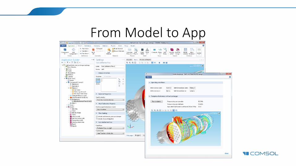
From Model to App

Running Apps
iPhone iPad
Web Browser COMSOL Client