Can Information Heterogeneity Explain
the Exchange Rate Determination
Puzzle? 1
Philippe Bacchetta
Study Center Gerzensee
University of Lausanne
CEPR
Eric van Wincoop
University of Virginia
NBER
April 8, 2004
1We would like to thank Bruno Biais, Gianluca Benigno, Margarida Duarte, Ken
Froot, Harald Hau, Olivier Jeanne, Richard Lyons, Elmar Mertens, and seminar partic-
ipants at the NBER IFM fall meeting, a CEPR-RTN workshop in Dublin, ESSFM in
Gerzensee, SIFR Conference in Stockholm, the New York and Boston Feds, the Board
of Governors, the ECB, CEMFI, the IMF, the Econometric Society Meetings in San
Diego and the Universities of Harvard, Princeton, Virginia, Boston College, UQAM,
Lausanne, North Carolina State, Georgetown, Wisconsin and Notre Dame for comments.
Bacchetta's work on this paper is part of a research network on `The Analysis of Inter-
national Capital Markets: Understanding Europe's role in the Global Economy,' funded
by the European Commission under the Research Training Network Program (Contract
No. HPRN-CT-1999-00067).

Abstract
Empirical evidence shows that observed macroeconomic fundamentals have little
explanatory power for nominal exchange rates (the exchange rate determination
puzzle). On the other hand, the recent \microstructure approach to exchange
rates" has shown that most exchange rate volatility at short to medium horizons is
related to order ow. In this paper we introduce symmetric information dispersion
about future fundamentals in a dynamic rational expectations model in order to
explain these stylized facts. Consistent with the evidence the model implies that
(i) observed fundamentals account for little of exchange rate volatility in the short
to medium run, (ii) over long horizons the exchange rate is closely related to
observed fundamentals, (iii) exchange rate changes are a weak predictor of future
fundamentals, and (iv) the exchange rate is closely related to order ow over both
short and long horizons.

I Introduction
The poor explanatory power of existing theories of the nominal exchange rate is
most likely the major weakness of international macroeconomics. Meese and Ro-
go� [1983] and the subsequent literature have found that a random walk predicts
exchange rates better than macroeconomic models in the short run. Lyons [2001]
refers to the weak explanatory power of macroeconomic fundamentals as the \ex-
change rate determination puzzle".1 This puzzle is less acute for long-run exchange
rate movements, since there is extensive evidence of a much closer relationship be-
tween exchange rates and fundamentals at horizons of two to four years (e.g., see
Mark [1995]). Recent evidence from the microstructure approach to exchange rates
suggests that investor heterogeneity might play a key role in explaining exchange
rate uctuations. In particular, Evans and Lyons [2002a] show that most short-
run exchange rate volatility is related to order ow, which in turn is associated
with investor heterogeneity.2 Since these features are not present in existing the-
ories, a natural suspect for the failure of current models to explain exchange rate
movements is the standard hypothesis of a representative agent.
The goal of this paper is to present an alternative to the representative agent
model that can explain the exchange rate determination puzzle and the evidence
on order ow. We introduce heterogenous information into a standard dynamic
monetary model of exchange rate determination. There is a continuum of investors
who di�er in two respects. First, they have symmetrically dispersed information
about future macroeconomic fundamentals.3 Second, they face di�erent exchange
rate risk exposure associated with non-asset income. This exposure is private infor-
mation and leads to hedge trades whose aggregate is unobservable. Our main �nd-
ing is that information heterogeneity disconnects the exchange rate from observed
1See Cheung et.al. [2002] for more recent evidence. The exchange rate determination puzzle
is part of a broader set of exchange rate puzzles that Obstfeld and Rogo� [2001] have called the
\exchange rate disconnect puzzle". This also includes the lack of feedback from the exchange
rate to the macro economy and the excess volatility of exchange rates (relative to fundamentals).2See also Rime [2001], Froot and Ramadorai [2002], Evans and Lyons [2002b] or Hau et al.
[2002].3We know from extensive survey evidence that investors have di�erent views about the macro-
economic outlook. There is also evidence that exchange rate expectations di�er substantially
across investors. See Chionis and MacDonald [2002], Ito [1990], Elliott and Ito [1999], and
MacDonald and Marsh [1996].
1

macroeconomic fundamentals in the short run, while there is a close relationship
in the long run. At the same time there is a close link between the exchange rate
and order ow over all horizons.
Our modeling approach integrates several strands of literature. First, it has
in common with most of the existing (open economy) macro literature that we
adopt a fully dynamic general equilibrium model, leading to time-invariant second
moments. Second, it has in common with the noisy rational expectations literature
in �nance that the asset price (exchange rate) aggregates private information of
individual investors, with unobserved shocks preventing average private signals
from being fully revealed by the price. The latter are modeled endogenously as
hedge trades in our model.4 Third, it has in common with the microstructure
literature of the foreign exchange market that private information is transmitted
to the market through order ow.5
Most models in the noisy rational expectations literature and microstructure
literature are static or two-period models.6 This makes them ill-suited to address
the disconnect between asset prices and fundamentals, which has a dynamic di-
mension since the disconnect is much stronger at short horizons. Even the few
dynamic rational expectation models in the �nance literature cannot be applied in
our context. Wang [1993, 1994] develops an in�nite horizon noisy rational expecta-
tions model. There are only two types of investors, one of which can fully observe
the variables a�ecting the equilibrium asset price. We believe that it is more ap-
propriate to consider cases where no class of investors has superior information and
where there is broader dispersion of information. Several papers make a step in
this direction by examining symmetrically dispersed information in a multi-period
model, but they only examine an asset with a single payo� at a terminal date.7
For the dynamic dimension of our paper, we rely on the important paper by
4Some recent papers in the exchange rate literature have introduced exogenous noise in the
foreign exchange market. However, they do not consider information dispersion about future
macro fundamentals. Examples are Hau [1998], Jeanne and Rose [2002], Devereux and Engel
[2002], Kollman [2002], and Mark and Wu [1998].5See Lyons [2001] for an overview of this literature.6See Brunnermeier [2001] for an overview.7See He and Wang [1995], Vives [1995], Foster and Viswanathan [1996] or Brennan and Cao
[1997]. The latter assume that private information is symmetrically dispersed among agents
within a country, while there is also asymmetric information between countries.
2

Townsend [1983]. Townsend analyzed a business cycle model with symmetrically
dispersed information. As is the case in our model, the solution exhibits in�nitely
higher order expectations (expectations of other agents' expectations).8 We adapt
Townsend's solution procedure to our model. The only application to asset pricing
we are aware of is Singleton [1987], who applies Townsend's method to a model
for government bonds with a symmetric information structure.9
The equilibrium price of our competitive noisy rational expectation model can
be determined by a Walrasian auctioneer. However, the equilibrium can also be
interpreted as the outcome of an order-driven auction market, whereby market
orders based on private information hit an outstanding limit order book. This
characterization resembles the electronic trading system that nowadays dominates
the foreign exchange market. We de�ne limit orders as orders that are condi-
tional on public information, including the exchange rate. Limit orders provide
liquidity to the market. Market orders take liquidity from the market and are asso-
ciated with private information. Order ow is equal to net market orders. Private
information is then transmitted to the market through order ow, while public
information leads to price changes without any actual trade. Not surprisingly,
the weak relationship in the model between short-run exchange rate uctuations
and publicly observed fundamentals is closely mirrored by the close relationship
between exchange rate uctuations and order ow.10
8Subsequent contributions have been mostly technical, solving the same model as in Townsend
[1983] with alternative methods. See Kasa [2000] and Sargent [1991]. Probably as a result of the
technical di�culty in solving these models, the macroeconomics literature has devoted relatively
little attention to heterogeneous information in the last two decades. This contrasts with the
1970s where, following Lucas [1972], there had been active research on rational expectations and
heterogeneous information (e.g., see King, 1982). Recently, information issues in the context of
price rigidity have again been brought to the forefront in contributions by Woodford [2003] and
Mankiw and Reis [2002].9In Singleton's model there is no information dispersion about the payo� structure on the
assets (in this case coupons on government bonds), but there is private information about whether
noise trade is transitory or persistent. The uncertainty is resolved after two periods.10In recent work closely related to ours, Evans and Lyons [2004] also introduce microstructure
features in a dynamic general equilibrium model in order to shed light on exchange rate puzzles.
There are three important di�erences in comparison to our approach. First, they adopt a quote-
driven market, while we model an order-driven auction market. Second, they assume that all
investors within one country have the same information, while there is asymmetric information
across countries. Third, their model is not in the noisy rational expectations tradition.
3

The dynamic implications of the model for the relationship between the ex-
change rate, observed fundamentals and order ow can be understood as follows.
In the short run, rational confusion plays an important role in disconnecting the
exchange rate from observed fundamentals. Investors do not know whether an
increase in the exchange rate is driven by an improvement in average private sig-
nals about future fundamentals or an increase in unobserved hedge trades. This
implies that unobserved hedge trades have an ampli�ed e�ect on the exchange
rate since they are confused with changes in average private signals about future
fundamentals.11 We show that a small amount of hedge trades can become the
dominant source of exchange rate volatility when information is heterogeneous,
while it has practically no e�ect on the exchange rate when investors have com-
mon information.
In the long run there is a close relationship between the exchange rate, ob-
served fundamentals and cumulative order ow. First, rational confusion gradu-
ally dissipates as investors learn more about future fundamentals.12 The impact
of unobserved hedge trades on the equilibrium price therefore gradually weakens,
leading to a closer long-run relationship between the exchange rate and observed
fundamentals. Second, when the fundamental has a permanent component the
exchange rate and cumulative order ow are closely linked in the long run. Private
information about permanent future changes in the fundamental is transmitted to
the market through order ow, so that order ow has a permanent e�ect on the
exchange rate.
The remainder of the paper is organized as follows. Section II describes the
model and solution method. Section III considers a special case of the model in
order to develop intuition for our key results. Section IV discusses the implications
of the dynamic features of the model. Section V presents numerical results based
on the general dynamic model and Section VI concludes.
11The basic idea of rational confusion can already be found in the noisy rational expectation
literature. For example, Gennotte and Leland [1990] and Romer [1993] argued that such rational
confusion played a critical role in amplifying non-informational trade during the stock-market
crash of October 19, 1987.12Another recent paper on exchange rate dynamics where learning plays an important role is
Gourinchas and Tornell [2004]. In that paper, in which there is no investor heterogeneity, agents
learn about the nature of interest rate shocks (transitory or persistent), but there is an irrational
misperception about the second moments in interest rate forecasts that never goes away.
4
II A Monetary Model with Information Disper-
sion
II.A Basic Setup
Our model contains the three basic building blocks of the standard monetary
model of exchange rate determination: (i) money market equilibrium, (ii) pur-
chasing power parity, and (iii) interest rate parity. We modify the standard mon-
etary model by assuming incomplete and dispersed information across investors.
Before describing the precise information structure, we �rst derive a general solu-
tion to the exchange rate under heterogeneous information, in which the exchange
rate depends on higher order expectations of future macroeconomic fundamentals.
This generalizes the standard equilibrium exchange rate equation that depends on
common expectations of future fundamentals.
Both observable and unobservable fundamentals a�ect the exchange rate. The
observable fundamental is the ratio of money supplies. We assume that investors
have heterogeneous information about future money supplies. The unobservable
fundamental takes the form of an aggregate hedge against non-asset income in
the demand for foreign exchange. This unobservable element introduces noise in
the foreign exchange market in the sense that it prevents investors from inferring
average expectations about future money supplies from the price.13 This trade
also a�ects the risk premium in the interest parity condition.
There are two economies. They produce the same good, so that purchasing
power parity holds:
pt = p�t + st (1)
Local currency prices are in logs and st is the log of the nominal exchange rate.
There is a continuum of investors in both countries on the interval [0,1]. We
assume that there are overlapping generations of agents who live for two periods
and make only one investment decision. This assumption signi�cantly simpli�es
the presentation, helps in providing intuition, and allows us to obtain an exact
solution to the model.14
13For alternative modeling of 'noise' from rational behavior, see Wang [1994], Dow and Gorton
[1995], and Spiegel and Subrahmanyam [1992].14In an earlier version of the paper, Bacchetta and van Wincoop [2003], we also consider
5

Investors in both economies can invest in four assets: money of their own
country, nominal bonds of both countries with interest rates it and i�t , and a
technology with �xed real return r that is in in�nite supply. We assume that one
economy is large and the other in�nitesimally small; variables from the latter are
starred. Bond market equilibrium is therefore entirely determined by investors in
the large country, on which we will focus. We also assume that money supply in
the large country is constant. It is easy to show that this implies a constant price
level pt in equilibrium, so that it = r. For ease of notation, we just assume a
constant pt. Money supply in the small country is stochastic.
The wealth wit of investors born at time t is given by a �xed endowment. At
time t + 1 these investors receive the return on their investments plus income
yit+1 from time t + 1 production. We assume that production depends both on
the exchange rate and on real money holdings fmit through the function y
it+1 =
�itst+1�fmit(ln(fmi
t)�1)=�.15 The coe�cient �it measures the exchange rate exposureof the non-asset income of investor i. We assume that �it is time varying and
known only to investor i. This will generate an idiosyncratic hedging term. Agent
i maximizes
�Eite� cit+1
subject to
cit+1 = (1 + it)wit + (st+1 � st + i�t � it)biF t � itfmi
t + yit+1
where biF t is invested in foreign bonds and st+1 � st + i�t � it is the log-linearizedexcess return on investing abroad.
Combining the �rst order condition for money holdings with money market
equilibrium in both countries we get
mt � pt = ��it (2)
m�t � p�t = ��i�t (3)
where mt and m�t are the logs of domestic and foreign nominal money supply.
an in�nite-horizon version. While this signi�cantly complicates the solution method, numerical
results are almost identical.15By introducing money through production rather than utility we avoid making money de-
mand a function of consumption, which would complicate the solution.
6

The demand for foreign bonds by investor i is:16
biF t =Eit(st+1)� st + i�t � it
�2t� bit (4)
where the conditional variance of next period's exchange rate is �2t , which is the
same for all investors in equilibrium. The hedge against non-asset income is rep-
resented by bit = �it.
We assume that the exchange rate exposure is equal to the average exposure
plus an idiosyncratic term, so that bit = bt + "it. We will only consider the limit-
ing case where the variance of "it approaches in�nity, so that knowing one's own
exchange rate exposure provides no information about the average exposure. This
assumption is only made for convenience. The results in the paper will not qual-
itatively change when we assume a �nite, but positive, variance of "it. The key
assumption is that the aggregate hedge component bt is unobservable. We assume
that the average exposure bt follows an AR(1) process:
bt = �bbt�1 + "bt (5)
where "bt � N(0; �2b ). While bt is an unobserved fundamental, the assumed autore-gressive process is known by all agents.
II.B Market Equilibrium and Higher Order Expectations
Since bonds are in zero net supply, market equilibrium is given byR 10 b
iF tdi = 0.
One way to reach equilibrium is to have a Walrasian auctioneer to whom investors
submit their demand schedule biF t. However, we show in the next section that the
same equilibrium can also be implemented by introducing a richer microstructure
in the form of an order-driven auction market. In that case we can relate the
exchange rate to order ow.
Market equilibrium yields the following interest arbitrage condition:
Et(st+1)� st = it � i�t + �2t bt (6)
where Et is the average rational expectation across all investors. The model is
summarized by (1), (2), (3), and (6). Other than the risk premium in the interest
16Here we implicitly assume that st+1 is normally distributed. We will see in section II.D that
the equilibrium exchange rate indeed has a normal distribution.
7
rate parity condition associated with non-observable trade, these equations are the
standard building blocks of the monetary model of exchange rate determination.
De�ning the observable fundamental as ft = (mt � m�t ), in Appendix A we
derive the following equilibrium exchange rate:
st =1
1 + �
1Xk=0
��
1 + �
�kEkt
�ft+k � � �2t+kbt+k
�(7)
where E0
t (xt) = xt, E1
t (xt+1) = Et(xt+1) and higher order expectations are de�ned
as
Ek
t (xt+k) = EtEt+1:::Et+k�1(xt+k): (8)
Thus, the exchange rate at time t depends on the fundamental at time t, the
average expectation at t of the fundamental at time t+1, the average expectation
at t of the average expectation at t + 1 of the fundamental at t + 2, etc. The
law of iterated expectations does not apply to average expectations. For example,
EtEt+1(st+2) 6= Et(st+2).17 This is a basic feature of asset pricing under hetero-
geneous expectations: the expectation of other investors' expectations matters.18
In a dynamic system, this leads to the in�nite regress problem, as analyzed in
Townsend [1983]: as the horizon goes to in�nity the dimensionality of the expec-
tation term goes to in�nity.
II.C The Information Structure
We assume that at time t investors observe all past and current ft, while they
receive private signals about ft+1; :::; ft+T . More precisely, we assume that investors
receive one signal each period about the observable fundamental T periods ahead.
For example, at time t investor i receives a signal
vit = ft+T + "vit "vit � N(0; �2v) (9)
17See Allen, Morris, and Shin [2003] and Bacchetta and van Wincoop [2004a].18Notice that the higher order expectations are of a dynamic nature, i.e., today's expectations
of tomorrow's expectations. This contrasts with most of the literature that considers higher
order expectations in a static context with strategic externalities, e.g., Morris and Shin [2002] or
Woodford [2003].
8
where "vit is independent from ft+T and other agents' signals.19 As usual in this
context we assume that the average signal received by investors is ft+T , i.e.,R 10 v
itdi = ft+T .
20
We also assume that the observable fundamental's process is known by all
agents and consider a general process:
ft = D(L)"ft "ft � N(0; �2f ) (10)
where D(L) = d1 + d2L + d3L + ::: and L is the lag operator. Since investors
observe current and lagged values of the fundamental, knowing the process provides
information about the fundamental at future dates.
II.D Solution Method
In order to solve the equilibrium exchange rate there is no need to compute all the
higher order expectations that it depends on. The key equation used in the solu-
tion method is the interest parity condition (6), which captures foreign exchange
market equilibrium. It only involves a �rst order average market expectation.
We adopt a method of undetermined coe�cients, conjecturing an equilibrium ex-
change rate equation and then verifying that it satis�es the equilibrium condition
(6). Townsend [1983] adopts a similar method for solving a business cycle model
with higher order expectations.21 Here we provide a brief description of the solu-
tion method, leaving details to Appendix B.
We conjecture the following equilibrium exchange rate equation that depends
on shocks to observable and unobservable fundamentals:
st = A(L)"ft+T +B(L)"
bt (11)
19This implies that each period investors have T signals that are informative about future
observed fundamentals. Note that the analysis could be easily extended to the case where
investors receive a vector of signals each period.20See Admati [1985] for a discussion.21The solution method described in Townsend [1983] applies to the model in section 8 of that
paper where the economy-wide average price is observed with noise. Townsend [1983] mistakenly
believed that higher order expectations are also relevant in a two-sector version of the model
where �rms observe each other's prices without noise. Pearlman and Sargent [2002] show that
the equilibrium fully reveals private information in that case.
9

where A(L) and B(L) are in�nite order polynomials in the lag operator L. The
errors "ivt do not enter the exchange rate equation as they average to zero across
investors. Since at time t investors observe the fundamental ft, only the innovations
"f between t+ 1 and t+ T are unknown. Similarly shocks "b between t� T and tare unknown. Exchange rates at time t� T and earlier, together with knowledgeof "f at time t and earlier, reveal the shocks "b at time t� T and earlier.Investors can then solve a signal extraction problem for the �nite number of un-
known innovations. Both private signals and exchange rates from time t�T +1 tot provide information about the unknown innovations. The solution to the signal
extraction problem leads to expectations at time t of the unknowns as a function
of observables, which in turn can be written as a function of the innovations them-
selves. One can then compute the average expectation of st+1. Substituting the
result into the interest parity condition (6) leads to a new exchange rate equation.
The coe�cients of the polynomials A(L) and B(L) can then be derived by solving
a �xed point problem, equating the coe�cients of the conjectured exchange rate
equation to those in the equilibrium exchange rate equation. Although the lag
polynomials are of in�nite order, for lags longer than T periods the information
dispersion plays no role and an analytical solution to the coe�cients is feasible.22
III Model Implications: A Special Case
In this section we examine the special case where T = 1, which has a relatively
simple solution. This example is used to illustrate how information heterogeneity
disconnects the exchange rate from observed macroeconomic fundamentals, while
establishing a close relationship between the exchange rate and order ow.
One aspect that simpli�es the solution for T = 1 is that higher order expec-
tations are the same as �rst order expectations. This can be seen as follows.
Bacchetta and van Wincoop [2004a] show that higher order expectations are equal
to �rst order expectations plus average expectations of future market expecta-
22In Bacchetta and van Wincoop [2003] we solve the model for the case where investors have
in�nite horizons. The solution is then complicated by the fact that investors also need to hedge
against changes in expected future returns. This hedge term depends on the in�nite state space,
which is truncated to obtain an approximate solution. Numerical results are almost identical to
the case of overlapping generations.
10
tional errors. For example, the second order expectation of ft+2 can be written as
E2tft+2 = Etft+2 + Et(Et+1ft+2 � ft+2). When T = 1 investors do not expect the
market to make expectational errors next period. An investor may believe at time
t that he has di�erent private information about ft+1 than others. However, that
information is no longer relevant next period since ft+1 is observed at t+ 1.23
While not critical, we make the further simplifying assumptions in this section
that bt and ft are i.i.d., i.e., �b = 0 and ft = "ft . Replacing higher order with �rst
order expectations, equation (7) then becomes:
st =1
1 + �
�ft +
�
1 + �Etft+1
�� �
1 + � �2bt (12)
Only the average expectation of ft+1 appears. We have replaced �2t with �
2 since
we will focus on the stochastic steady state where second order moments are time-
invariant.
III.A Solving the Model with Heterogenous Information
When T = 1 investors receive private signals vit about ft+1, as in (9). Therefore
the average expectation Etft+1 in (12) depends on the average of private signals,
which is equal to ft+1 itself. This implies that the exchange rate st depends on
ft+1, so that the exchange rate becomes itself a source of information about ft+1.
However, the exchange rate is not fully revealing as it also depends on unobserved
aggregate hedge trades bt. To determine the information signal about ft+1 provided
by the exchange rate we need to know the equilibrium exchange rate equation. We
conjecture that
st =1
1 + �ft + �fft+1 + �bbt (13)
Since an investor observes ft, the signal he gets from the exchange rate can be
written est�f= ft+1 +
�b�fbt (14)
where est = st� 11+�ft is the "adjusted" exchange rate. The variance of the error of
this signal is (�b=�f )2�2b . Consequently, investor i infers E
itft+1 from three sources
of information: i) the distribution of ft+1; ii) the signal vit; iii) the adjusted exchange
23See Bacchetta and van Wincoop [2004a] for a more detailed discussion of this point.
11
rate (i.e., (14)). Since errors in each of these signals have a normal distribution,
the projection theorem implies that Eitft+1 is given by a weighted average of the
three signals, with the weights determined by the precision of each signal. We
have:
Eitft+1 =�vvit + �
sest=�fD
(15)
where �v = 1=�2v , �s = 1=(�b=�f )
2�2b , �f = 1=�2f , and D = 1=var(ft+1) = �v +
�f + �s. For the exchange rate signal, the precision is complex and depends both
on �2b and �b=�f , the latter being endogenous. By substituting (15) into (12) and
using the fact thatR 10 v
itdi = ft+1 in computing Etft+1, we get:
st =1
1 + �ft + z
�
(1 + �)2�v
Dft+1 � z
�
1 + � �2bt (16)
where z = 1=(1 � �(1+�)2
�s
�fD) > 1. Equation (16) con�rms the conjecture (13).
Equating the coe�cients on ft+1 and bt in (16) to respectively �f and �b yields
implicit solutions to these parameters.
We will call z the magni�cation factor: the equilibrium coe�cient of bt in (16)
is the direct e�ect of bt in (12) multiplied by z. This magni�cation can be ex-
plained by rational confusion. When the exchange rate changes, investors do not
know whether this is driven by hedge trades or by information about future macro-
economic fundamentals by other investors. Therefore, they always revise their ex-
pectations of fundamentals when the exchange rate changes (equation (15)). This
rational confusion magni�es the impact of the unobserved hedge trades on the ex-
change rate. More speci�cally, from (12) and (15), we can see that a change in bt
has two e�ects on st. First, it a�ects st directly in (12) through the risk-premium
channel. Second, this direct e�ect is magni�ed by an increase in Etft+1 from (15).
The magni�cation factor can be written as24
z = 1 +�s
�v(17)
The magni�cation factor therefore depends on the precision of the exchange rate
signal relative to the precision of the private signal. The better the quality of the
exchange rate signal, the more weight is given to the exchange rate in forming
24Substitute �f = z�
(1+�)2�v
D into z = 1=(1� �(1+�)2
�s
�fD) and solve for z.
12
expectations of ft+1, and therefore the larger the magni�cation of the unobserved
hedge trades.
Figure 1 shows the impact of two key parameters on magni�cation. A rise
in the private signal variance �2v at �rst raises magni�cation and then lowers it.
Two opposite forces are at work. First, an increase in �2v reduces the precision �v
of the private signal. Investors therefore give more weight to the exchange rate
signal, which enhances the magni�cation factor. Second, a rise in �2v implies less
information about next period's fundamental and therefore a lower weight of ft+1
in the exchange rate. This reduces the precision �s of the exchange rate signal,
which reduces the magni�cation factor. For large enough �2v this second factor
dominates. The magni�cation factor is therefore largest for intermediate values
of the quality of private signals. Figure 1 also shows that a higher variance �2b of
hedging shocks always reduces magni�cation. It reduces the precision �s of the
exchange rate signal.
III.B Disconnect from Observed Fundamentals
In order to precisely identify the channels through which information heterogeneity
disconnects the exchange rate from observed fundamentals, we now compare the
model to a benchmark with identically informed investors. The benchmark we
consider is the case where investors receive the same signal on future ft's, i.e., they
have incomplete but common knowledge on future fundamentals. With common
knowledge all investors receive the signal
vt = ft+T + "vt "vt � N(0; �2v;c) (18)
where "vt is independent of ft+T .
De�ning the precision of this signal as �v;c � 1=�2v;c, the conditional expectationof ft+1 is
Eitft+1 = Etft+1 =�v;cvtd
(19)
where d � 1=vart(ft+1) = �v;c + �f . Substitution into (12) yields the equilibriumexchange rate:
st =1
1 + �ft + �vvt + �
cbbt (20)
where �v =�
(1+�)2�v;c=d, and �cb = � �
1+� �2c . Here �
2c is the conditional variance
of next period's exchange rate in the common knowledge model. In this case the
13
exchange rate is fully revealing, since by observing st investors can perfectly deduce
bt. Thus, �cb is equal to the direct risk-premium e�ect of bt given in (12).
We can now compare the connection between the exchange rate and observed
fundamentals in the two models. In the heterogeneous information model the ob-
served fundamental is ft, while in the common knowledge model it also includes vt.
We compare the R2 of a regression of the exchange rate on observed fundamentals
in the two models. From (13), the R2 in the heterogeneous information model is
de�ned by:
R2
1�R2 =1
(1+�)2�2f
�2f�2f + z
2�
�1+�
�2 2�4�2b
(21)
>From (20) the R2 in the common knowledge model is de�ned by:
R2
1�R2 =1
(1+�)2�2f + �
2v(�
2f + �
2v;c)�
�1+�
�2 2�4c�
2b
(22)
If the conditional variance of the exchange rate is the same in both models the R2
is clearly lower in the heterogeneous information model. Two factors contribute
to this. First, the contribution of unobserved trades to exchange rate volatility is
ampli�ed, as measured by the magni�cation factor z in the denominator of (21).
Second, the average signal in the heterogeneous information model, which is equal
to the future fundamental, is unobserved and therefore contributes to reducing
the R2. It also appears in the denominator of (21). In contrast, the signal about
future fundamentals is observed in the common knowledge model, and therefore
contributes to raising the R2. The variance of this signal, �2f + �2v;c, appears in the
numerator of (22). The conditional variance of the exchange rate also contributes
to the R2. It can be higher in either model, dependent on assumptions about
parameter values and quality of the public and private signals.
III.C Order Flow
Evans and Lyons [2002a] de�ne order ow as \the net of buyer-initiated and seller-
initiated orders." While each transaction involves a buyer and a seller, the sign of
the transaction is determined by the initiator of the transaction. The initiator of
a transaction is the trader (either buyer or seller) who acts based on new private
information. Here private information is broadly de�ned. In our setup it includes
14

both private information about the future fundamental and private information
that leads to hedge trades. The passive side of trade varies across models. In
a quote-driven dealer market, such as modeled by Evans and Lyons [2002a], the
quoting dealer is on the passive side. The foreign exchange market has traditionally
been characterized as a quote-driven multi-dealer market, but the recent increase
in electronic trading (e.g., EBS) implies that a majority of trade is done through
an auction market. In that case the limit orders are the passive side of transactions
and provide liquidity to the market. The initiated orders are referred to as market
orders that are confronted with the passive outstanding limit order book.
In our modeling of order ow we think of the foreign exchange market as an
auction market. We split the demand biF;t by investor i into order ow (market or-
ders) and limit orders. Limit orders are associated with the component of demand
that depends on the price (exchange rate) and common information. These are
passive orders that are only executed when confronted with market orders. Mar-
ket orders are associated with the component of demand that depends on private
information.25
Using (4), (13) and (15), we can write total demand by individual i as
biF;t =1 + �
� �2z
�1
1 + �ft � st
�+
�v
(1 + �) �2Dvit � bit (23)
Limit orders are captured by the �rst term, while order ow is captured by the
sum of the last two terms. If there were no private information, so that the last
two terms are equal to their unconditional mean of zero, demand would be the
same for all investors. Since aggregate supply is zero, the holdings of each investor
would always be zero. In that case the exchange rate may change due to new
25One way to formalize this separation into limit and market orders is to introduce foreign
exchange dealers to whom investors delegate price discovery. Dealers are simply a veil, passing
on customer orders to the interdealer market, where price discovery takes place. Customers
submit their demand functions to dealers through a combination of limit and market orders.
Dealers can place both types of orders in the interdealer electronic auction market, but need to
place the limit orders before customer orders are known. If we introduce an in�nitesimal trading
cost in the interdealer market that is proportional to the volume of executed trades, dealers will
submit limit orders that are equal to the expected customer orders based on public information.
The unexpected customer orders are associated with private information and are submitted as
market orders to the interdealer market. This formalization also connects well to the existing
data, which is for interdealer order ow.
15

public information (st = ft=(1 + �)), but this happens without any transactions
in the foreign exchange market.
In the presence of private information there is trade in the foreign exchange
market. We de�ne �xit as order ow of investor i, the sum of the last two terms on
the right hand side of (23).26 Aggregate order ow �xt =R 10 �x
itdi is then equal
to
�xt =�v
(1 + �) �2Dft+1 � bt (24)
Taking the aggregate of (23), imposing market equilibrium, we get
st =1
1 + �ft + z
�
1 + � �2�xt (25)
Equation (25) shows that the exchange rate is related in a simple way to a
commonly observed fundamental and order ow. The order ow term captures
the extent to which the exchange rate changes due to the aggregation of private
information. The impact of order ow is larger the bigger the magni�cation factor
z. A higher level of z implies that the order ow is more informative about the
future fundamental.
It is easily veri�ed that in the common knowledge model
st =1
1 + �ft + �vvt +
�
1 + � �2�xt (26)
In that case order ow is only driven by hedge trades. Since these trades have
no information content about future fundamentals, the impact of order ow on
the exchange rate is smaller (not multiplied by the magni�cation factor z). A
comparison between (25) and (26) clearly shows that the exchange rate is more
closely connected to order ow in the heterogeneous information model and more
closely connected to public information in the common knowledge model.
Equations (25) and (26) are di�erent from the speci�cation used in empirical
analysis, where the exchange rate is usually in �rst di�erences. The reason is that
in this section st is stationary, while in the data it is non-stationary. If we assume
that ft follows a random walk in the above example, we obtain an equation that is
26More generally, when the fundamentals are not i.i.d., the expectations of vit and bit based on
public information are non-zero. For example, when f follows a random walk the expectation of
vit based on public information is ft. In that case order ow is de�ned as the linear combination
of vit and bit in the demand b
iF;t that is orthogonal to public information.
16
close to the one used in empirical analyses.27 In the numerical analysis of Section
V, st is non-stationary and we run regressions in di�erences.
A related point is that when the fundamental f is non-stationary, order ow
associated with private information about future fundamentals has a permanent
impact on the exchange rate. It is not the case though that cumulative order ow
and the exchange rate are cointegrated. Hedge trades have a transitory impact on
the exchange rate, but a permanent e�ect on cumulative order ow. This point is
made more precise in Appendix D for the case where f follows a random walk.28
IV Model Implications: Dynamics
In this section, we examine the more complex dynamic properties of the model
when T > 1. There are two important implications. First, it creates endogenous
persistence of the impact of non-observable shocks on the exchange rate. Second,
higher order expectations di�er from �rst order expectations when T > 1. Even
for T = 2 expectations of in�nite order a�ect the exchange rate. We show that
higher order expectations tend to increase the magni�cation e�ect, but have an
ambiguous impact on the disconnect. We now examine these two aspects in turn.
IV.A Persistence
When T > 1, even transitory non-observable shocks have a persistent e�ect on the
exchange rate. This is caused by the combination of heterogeneous information
and the positive weight given to information from previous periods in forming ex-
pectations. The exchange rate at time t depends on future fundamentals ft+1, ft+2,
:::,ft+T , and therefore provides information about each of these future fundamen-
tals. A transitory unobservable shock to bt a�ects the exchange rate at time t and
27More precisely, in this case we would �nd �st = (1��f )�ft+z �1+� �
2t�xt��b"bt�1. When
both b and f follow random walks we obtain an equation for the common knowledge model very
similar to that implied by the model of Evans and Lyons [2002a]: �st = �ft + � �2t�xt. Their
model is indeed one where both \portfolio shifts" �bt and changes in observed fundamentals �ft
are permanent and agents do not have private information about future fundamentals.28It also holds in this section, where f is stationary. In that case the exchange rate is stationary,
but cumulative order ow is non-stationary since transitory hedge trades have a permanent e�ect
on cumulative order ow.
17
therefore a�ects the expectations of all future fundamentals up to time t+T . This
rational confusion will last for T periods, until the �nal one of these fundamentals,
ft+T , is observed. Until that time investors will continue to give weight to st in
forming their expectations of future fundamentals, so that bt continues to a�ect
the exchange rate.29 As investors gradually learn more about ft+1, ft+2, :::,ft+T ,
both by observing them and through new signals, the impact on the exchange rate
of the shock to bt gradually dissipates.
The persistence of the impact of b-shocks on the exchange rate is also a�ected
by the persistence of the shock itself. When the b-shock itself becomes more
persistent, it is more di�cult for investors to learn about fundamentals up to time
t+T from exchange rates subsequent to time t. The rational confusion is therefore
more persistent and so is the impact of b-shocks on the exchange rate.
IV.B Higher Order Expectations
The topic of higher order expectations is a di�cult one, but it has potentially
important implications for asset pricing. Since a detailed analysis falls outside the
scope of this paper, we limit ourselves to a brief discussion regarding the impact
of higher order expectations on the connection between the exchange rate and ob-
served fundamentals. We apply the results of Bacchetta and van Wincoop [2004a],
where we provide a general analysis of the impact of higher order expectations on
asset prices.30 We still assume that �b = 0.
Let st denote the exchange rate that would prevail if the higher order expec-
tations in (7) are replaced by �rst order expectations.31 In Bacchetta and van
Wincoop [2004a] we show that the present value of the di�erence between higher
and �rst order expectations depends on average �rst-order expectational errors
about average private signals. In Appendix C we show that in our context this
29This result is related to �ndings by Brown and Jennings [1989] and Grundy and McNichols
[1989], who show in the context of two-period noisy rational expectations models that the asset
price in the second period is a�ected by the asset price in the �rst period.30Allen, Morris and Shin [2003] also provide an insightful analysis of higher order expectations
with an asset price, but they do not consider an in�nite horizon model.
31That is st =1
1+�
P1k=0
��1+�
�kEt�ft+k � � �2t+kbt+k
�
18

leads to
st = st +1
1 + �
TXk=2
�k(Etft+k � ft+k) (27)
The parameters �k are de�ned in the Appendix and are positive in all numeri-
cal applications. Higher order expectations therefore introduce a new asset price
component, which depends on average �rst-order expectational errors about future
fundamentals.
Moreover, the expectational errors Etft+k�ft+k depend on errors in public sig-nals; based on private information alone these average expectational errors would
be zero. There are two types of errors in public signals. First, there are errors in
the exchange rate signals that are caused by the unobserved hedge trades at time
t and earlier. This implies that unobserved hedge trades receive a larger weight
in the equilibrium exchange rate. The other type of errors in public signals are
errors in the signals based on the process of ft. These errors depend negatively
on future innovations in the fundamental, which implies that the exchange rate
depends less on unobserved future fundamentals. To summarize, hedge shocks are
further magni�ed by the presence of higher order expectations, while the overall
impact on the connection between the exchange rate and observed fundamentals
is ambiguous.32
V Model Implications: Numerical Analysis
We now solve the model numerically to illustrate the various implications of the
model discussed above. We �rst consider a benchmark parameterization and then
discuss the sensitivity of the results to changing some key parameters.
V.A A Benchmark Parameterization
The parameters of the benchmark case are reported in Table 1. They are chosen
mainly to illustrate the potential impact of information dispersion; they are not
calibrated or chosen to match any data moments. We assume that the observable
32In Bacchetta and van Wincoop [2004a], we show that the main impact of higher order
expectations is to disconnect the price from the present value of future observable fundamentals.
19

fundamental f follows a random walk, whose innovations have a standard devia-
tion of �f = 0:01. We assume that the extent of private information is small by
setting a high standard deviation of the private signal error of �v = 0:08. The
unobservable fundamental b follows an AR process with autoregressive coe�cient
of �b = 0:8 and a standard deviation �b = 0:01 of innovations. Although we have
made assumptions about both �b and risk-aversion , they enter multiplicatively in
the model, so only their product matters. Finally, we assume T = 8, so that agents
obtain private signals about fundamentals eight periods before they are realized.
Figure 2 shows some of the key results from the benchmark parameterization.
Panels A and B show the dynamic impact on the exchange rate in response to one-
standard deviation shocks in the private and common knowledge models. In the
heterogeneous agent model, there are two shocks: a shock "ft+T (f -shock), which
�rst a�ects the exchange rate at time t, and a shock "bt (b-shock). In the common
knowledge model there are also shocks "vt , which a�ect the exchange rate through
the commonly observable fundamental vt. In order to facilitate comparison, we set
the precision of the public signal such that the conditional variance of next period's
exchange rate is the same as in the heterogeneous information model. This implies
that the unobservable hedge trades have the same risk-premium e�ect in the two
models. We will show below that our key results do not depend on the assumed
precision of the public signal.
Magni�cation
The magni�cation factor in the benchmark parameterization turns out to be
substantial: 7.2. This is visualized in Figure 2 by comparing the instantaneous
response of the exchange rate to the b-shocks in the two models in panels A and
B. The only reason the impact of a b-shock is so much bigger in the heteroge-
neous information model is the magni�cation factor associated with information
dispersion.
Persistence
We can see from panel A that after the initial shock the impact of the b-shocks
dies down almost as a linear function of time. The half-life of the impact of the
shock is 3 periods. After 8 periods the rational confusion is resolved and the impact
is the same as in the public information model, which is close to zero.
20

The meaning of a 3-period half-life depends of course on what we mean by a
period in the model. What is critical is not the length of a period, but the length
of time it takes for uncertainty about future macro variables to be resolved. For
example, assume that T is eight months. If a period in our model is a month,
then T = 8. If a period is three days, then T = 80. We �nd that the half-life
of the impact of the unobservable hedge shocks on the exchange rate that can be
generated by the model remains virtually unchanged as we change the length of a
period. For T = 8 the half life is about 3, while for T = 80 it is about 30.33 In
both cases the half-life is 3 months. Persistence is therefore driven critically by the
length of time it takes for uncertainty to resolve itself. Deviations of the exchange
rate from observed fundamentals can therefore be very long-lasting when it takes
a long time before expectations about future fundamentals can be validated, such
as expectations about the long-term technology growth rate of the economy.
Exchange rate disconnect in the short and the long run
Panel C reports the contribution of unobserved hedge trades to the variance of
st+k�st at di�erent horizons. In the heterogeneous information model, 70% of thevariance of a 1-period change in the exchange rate is driven by the unobservable
hedge trades, while in the common knowledge model it is a negligible 1.3%. While
in the short-run unobservable fundamentals dominate exchange rate volatility, in
the long-run observable fundamentals dominate. For example, the contribution of
hedge trades to the variance of exchange rate changes over a 10-period interval is
less than 20%. As seen in panel A, the impact of hedge trades on the exchange
rate gradually dies down as rational confusion dissipates over time.
In order to determine the relationship between exchange rates and observed
fundamentals, panel D reports the R2 of a regression of st+k � st on all currentand lagged observed fundamentals. In the heterogeneous information model this
includes all one period changes in the fundamental f that are known at time
33When we change the length of a period we also need to change other model parameters,
such as the standard deviations of the shocks. In doing so we restrict parameters such that (i)
the contribution of b-shocks to var(st+1 � st) is the same as in the benchmark parameterizationand (ii) the impact of b-shocks on exchange rate volatility remains largely driven by information
dispersion (large magni�cation factor). For example, when we change the benchmark parame-
terization such that T = 80, �v = 0:26, �f = 0:0016 and � = 44, the half-life is 28 periods. The
magni�cation factor is 48.
21
t + k: ft+s � ft+s�1, for s � k. In the common knowledge model it also includesthe corresponding one-period changes in the public signal v. The R2 is close to
1 for all horizons in the common knowledge model, while it is much lower in the
heterogeneous information model. At the one-period horizon it is only 0.14; it then
rises as the horizon increases, to 0.8 for a 20-period horizon. This is consistent
with extensive �ndings that macroeconomic fundamentals have weak explanatory
power for exchange rates in the short to medium run, starting with Meese and
Rogo� [1983], and �ndings of a closer relationship over longer horizons.34
Two factors account for the results in panel D. The �rst is that the relative
contribution of unobservable hedge shocks to exchange rate volatility is large in
the short-run and small in the long-run, as illustrated in panel C. The second
factor is that through private signals the exchange rate at time t is also a�ected by
innovations "ft+1; ::; "ft+T in future fundamentals that are not yet observed today. In
the long-run these become observable, again contributing to a closer relationship
between the exchange rate and observed fundamentals in the long-run.
Exchange rate and future fundamentals
Recently Engel and West [2002] and Froot and Ramadorai [2002] have reported
evidence that exchange rate changes predict future fundamentals, but only weakly
so. Our model is consistent with these �ndings. Panel E of Figure 2 reports the
R2 of a regression ft+k � ft+1 on st+1 � st for k � 2. The R2 is positive, but is
never above 0.14. The exchange rate is a�ected by the private signals of future
fundamentals, which aggregate to the future fundamentals. However, most of the
short-run volatility of exchange rates is associated with unobservable hedge trades,
which do not predict future fundamentals.
Exchange rate and order ow
Order ow is again de�ned as the component of demand for foreign bonds
that is orthogonal to public information (other than the yet to be determined
st). Details of how it is computed are discussed in Appendix D. With xt de�ned
as cumulative order ow, panel F reports the R2 of a regression of st+k � st onxt+k � xt. The R2 is large and rises with the horizon from 0.84 for k = 1 to
34See MacDonald and Taylor [1993], Mark [1995], Chinn and Meese [1995], Mark and Sul
[2001], Froot and Ramadorai [2002] and Gourinchas and Rey [2004].
22
0.97 for k = 40. Although it appears that the R2 approaches 1 as k approaches
in�nity, it asymptotically reaches a level near 0.99.35 We show in the Appendix
that cumulative order ow and the exchange rate are not cointegrated. Both
the exchange rate and cumulative order ow depend on ft. However, cumulative
order ow also depends on the in�nite sum of all past hedge demand innovations,
while the coe�cient on past hedge innovations in the equilibrium exchange rate
approaches zero for long lags.
It is important to point out that the close relationship between the exchange
rate and order ow in the long run is not inconsistent with the close relationship
between the exchange rate and observed fundamentals in the long run. When the
exchange rate rises due to private information about permanently higher future
fundamentals, the information reaches the market through order ow. Eventually
the future fundamentals will be observed, so that there is a link between the
exchange rate and the observed fundamentals. But most of the information about
higher future fundamentals is aggregated into the price through order ow. Order
ow associated with information about future fundamentals has a permanent e�ect
on the exchange rate.
Our results can be compared to similar regressions that have been conducted
based on the data. Evans and Lyons [2002a] estimate regressions of one-day ex-
change rate changes on daily order ow. They �nd an R2 of 0.63 and 0.40 for
respectively the DM/$ and the yen/$ exchange rate, based on four months of daily
data in 1996. Evans and Lyons [2002b] report results for nine currencies. They
point out that exchange rate changes for any currency pair can also be a�ected
by order ow for other currency pairs. Regressing exchange rate changes on order
ow for all currency pairs they �nd an average R2 of 0.67 for their nine currencies.
The pictures for the exchange rate and cumulative order ow reported in Evans
and Lyons [2002a] suggest that the link is even stronger over horizons longer than
one day, although their dataset is too short to formally run such regressions.
The strong link between order ow and exchange rates in both the model
and the data implies that most information reaches the market through order
ow, and is therefore private information rather than public information. While
35The relationship between st+k � st and xt+k � xt does not always get stronger for longerhorizons. For low values of T the R2 declines with k and then converges asymptotically to a
positive level.
23

not reported in panel F, the R2 of regressions of exchange rate changes on order
ow in the public information model is close to zero. Two factors contribute to
the much closer link between order ow and exchange rates in the heterogeneous
information model. First, in the heterogenous information model both private
information about future fundamentals and hedge trades contribute to order ow,
while in the public information model only hedge trades contribute to order ow.
Second, the impact on the exchange rate of the order ow due to hedge trades is
much larger in the heterogeneous information model. The reason is that order ow
is informative about future fundamentals in the heterogeneous information model.
As illustrated in section III.C, the magni�cation factor z applied to the impact
of b-shocks on the exchange rate also applies to the impact of order ow on the
exchange rate.
Figure 3 reports simulations of the exchange rate and cumulative order ow over
40 periods. The Figure shows four simulations, based on di�erent random draws of
the observable and unobservable fundamentals.36 The simulations con�rm a close
link between the exchange rate and cumulative order ow at both short and long
horizons. Some of these pictures look quite similar to those reported by Evans and
Lyons [2002a] for the DM/$ and yen/$.
V.B Sensitivity to Model Parameters
In this subsection, we consider the parameter sensitivity of two key moments: the
R2 of a regression of st+1 � st on observed fundamentals at t + 1 and earlier andthe R2 of a regression of st+1 � st on order ow xt+1 � xt. These are the momentsreported for k = 1 in panels D and F of Figure 2.
A �rst issue is that the precision of the public signal in the common knowledge
model does not play an important role in the comparison with the heterogeneous
information model. In particular, it has little in uence on the stark di�erence
between the two models regarding the connection between the exchange rate and
observed fundamentals. Consider the R2 of a regression of a one-period change in
the exchange rate on all current and past observed fundamentals, as reported in
Figure 2D. In the heterogeneous information model it is 0.14, while in the public
36Both the log of the exchange rate and cumulative order ow are set at zero at the start of
the simulation.
24

information model it varies from 0.97 to 0.99 as we change the variance of the noise
in the public signal from in�nity to zero.37
We now consider sensitivity analysis to four key model parameters in the het-
erogeneous information model: �v, �b, �b and T . The results are reported in Figure
4. Not surprisingly, the two R2's are almost inversely related as we vary parame-
ters. The larger the impact of order ow as a channel through which information
is transmitted to the market, the smaller is the explanatory power of commonly
observed macro fundamentals.38
An increase in �v, implying less precise private information, reduces the link
between the exchange rate and order ow and increases the link between the ex-
change rate and observed fundamentals. In the limit as the noise in private signals
approaches in�nity, the heterogeneous information model approaches the public
information model (with uninformative signals).
Somewhat surprisingly, an increase in the noise originating from hedge trades,
by either raising the standard deviation �b or the persistence �b, tends to strengthen
the link between the exchange rate and observed fundamentals and reduce the
link between the exchange rate and order ow. However, the e�ect is relatively
small due to o�setting factors. Order ow becomes less informative about future
fundamentals with more noisy hedge trades. This reduces the impact of order ow
on the exchange rate. On the other hand, the volatility of order ow increases,
which contributes positively to the R2 for order ow. The former e�ect slightly
dominates.
It is also worthwhile pointing out that the assumed stationarity of hedge trades
in the benchmark parameterization is not responsible for the much weaker rela-
tionship between the exchange rate and observed fundamentals in the short-run
than the long-run. Even if we assume �b = 1, so that unobserved aggregate hedge
trades follow a random walk as well, this �nding remains largely unaltered. The
37In Figure 2, we have assumed that the precision of the public signal is such that the con-
ditional variance of the exchange rate is the same in the two models. This implies a standard
deviation of the error in the public signal of 0.033.38The two lines do not add to one. The reason is that some variables that are common
knowledge are not included in the regression on observed fundamentals. These are past exchange
rates and hedge demand T periods ago. Past exchange rates are not included since they are not
traditional fundamentals. Hedge demand T periods ago can be indirectly derived from exchange
rates T periods ago and earlier, but is not a directly observable fundamental.
25
R2 for observed fundamentals rises from 0.21 for a 1-period horizon to 0.85 for a
40-period horizon.
The �nal panel of Figure 4 shows the impact of changing T . Initially, an
increase in T leads to a closer link between order ow and the exchange rate and
a weaker link between observed fundamentals and the exchange rate. The reason
is that as T increases the quality of private information improves because agents
have signals about fundamentals further into the future. This implies that the
impact of order ow on the exchange rate increases. Moreover, order ow itself
also becomes more volatile as more private information is aggregated. However,
beyond a certain level of T , the link between the exchange rate and order ow
is weakened when T is raised further. The reason is that the improved quality
of information reduces the conditional variance �2 of next period's exchange rate.
This reduces the e�ect of order ow on the exchange rate, as can be seen from
(25).
VI Conclusion
The close relationship between order ow and exchange rates, as well as the large
volume of trade in the foreign exchange market, suggest that investor heterogeneity
is key to understanding exchange rate dynamics. In this paper we have explored
the implications of information dispersion in a simple model of exchange rate de-
termination. We have shown that these implications are rich and that investors'
heterogeneity can be an important element in explaining the behavior of exchange
rates. In particular, the model can account for some important stylized facts on
the relationship between exchange rates, fundamentals and order ow: (i) fun-
damentals have little explanatory power for short to medium run exchange rate
movements, (ii) over long horizons the exchange rate is closely related to observed
fundamentals, (iii) exchange rate changes are a weak predictor of future funda-
mentals, and (iv) the exchange rate is closely related to order ow.
The paper should be considered only as a �rst step in a promising line of
research. A natural next step is to confront the model to the data. While the
extent of information dispersion and unobservable hedge trades are not known,
they both a�ect order ow. Some limited data on order ow are now available
and will help tie down the key model parameters. The magni�cation factor may
26
be quite large. Back-of-the-envelope calculations by Gennotte and Leland [1990]
in the context of a static model for the U.S. stock market crash of October 1987
suggest that the impact of a $6 billion unobserved supply shock was magni�ed by
a factor 250 due to rational confusion about the source of the stock price decline.
In the context of foreign exchange markets, Osler [2003] presents evidence that
trades which are uninformative about future fundamentals can have a very large
impact on the price.
There are several directions in which the model can be extended. The �rst is
to explicitly model nominal rigidities as in the \new open economy macro" litera-
ture. In that literature exchange rates are entirely driven by commonly observed
macro fundamentals. Conclusions that have been drawn about optimal monetary
and exchange rate policies are likely to be substantially revised when introducing
investor heterogeneity. Another direction is to consider alternative information
structures. For example, the information received by agents may di�er in its qual-
ity or in its timing. There can also be heterogeneity about the knowledge of the
underlying model. For example, in Bacchetta and van Wincoop [2004b], we show
that if investors receive private signals about the persistence of shocks, the impact
of observed variables on the exchange rate varies over time. The rapidly grow-
ing body of empirical work on order ow in the foreign exchange microstructure
literature is likely to increase our understanding of the nature of the information
structure, providing guidance to future modeling.
27
Appendix
A Derivation of equation (7)
It follows from (1), (2), (3), and (6) that
st =1
1 + �ft �
�
1 + � �2t bt +
�
1 + �E1t (st+1) (28)
Therefore
E1t (st+1) =
1
1 + �E1t (ft+1)�
�
1 + � �2t+1E
1t (bt+1) +
�
1 + �E2t (st+2) (29)
Substitution into (28) yields
st =1
1 + �
�ft � �2t bt +
�
1 + �E1t
�ft+1 � �2t+1bt+1
��+�
�
1 + �
�2E2t (st+2) (30)
Continuing to solve for st this way by forward induction and assuming a no-bubble
solution yields (7).
B Solution method with two-period overlapping
investors
The solution method is related to Townsend (1983, section VIII). We start with the
conjectured equation (11) for st and check whether it is consistent with the model,
in particular with equation (6). For this, we need to estimate the conditional
moments of st+1 and express them as a function of the model's innovations. Finally
we equate the parameters from the resulting equation to the initially conjectured
equation.
B.1 The exchange rate equation
>From (1)-(3), and the de�nition of ft, it is easy to see that i�t � it = (ft � st)=�.
Thus, (6) gives (for a constant �2t ):
st =�
1 + �Et(st+1) +
ft1 + �
� �
1 + � bt�
2 (31)
28

We want to express (31) in terms of current and past innovations. First, we have
ft = D(L)"ft , where D(L) = d1 + d2L + d3L + :::. Second, using (5) we can write
bt = C(L)"bt , where C(L) = 1 + �bL + �
2bL
2 + :::. What remains to be computed
are E(st+1) and �2.
Applying (11) to st+1, decomposing A(L) and B(L), we have
st+1 = a1"ft+T+1 + b1"
bt+1 + �
0�t + A�(L)"ft +B
�(L)"bt�T (32)
where �0t = ("ft+T ; :::; "ft+1; "
bt ; :::; "
bt�T+1) represents the vector of unobservable in-
novations, �0 = (a2; a3; :::; aT+1; b2; :::; bT+1) and A�(L) = aT+2 + aT+3L + :::(with
a similar de�nition for B�(L)). Thus, we have (since "fj and "bj�T are known for
j � t):Eit(st+1) = �
0Eit(�t) + A�(L)"ft +B
�(L)"bt�T (33)
�2 = vart(st+1) = a21�2f + b
21�2b + �
0vart(�t)� (34)
We need to estimate the conditional expectation and variance of the unobserv-
able �t as a function of past innovations.
B.2 Conditional moments
We follow the strategy of Townsend (1983, p.556), but use the notation of Hamilton
[1994, chapter 13]. First, we subtract the known components from the observables
st and vit and de�ne these new variables as s�t and v
i�t . Let the vector of these
observables be Yit =
�s�t ; s
�t�1; :::; s
�t�T+1; v
i�t ; :::; v
i�t�T+1
�. From (32) and (9), we
can write:
Yit = H
0�t +wit (35)
where wit = (0; :::; 0; "
vit ; :::; "
vit�T+1)
0 and
H0 =
2666666666666666664
a1 a2 ::: aT b1 b2 ::: bT
0 a1 ::: aT�1 0 b1 ::: bT�1
::: ::: ::: ::: ::: ::: ::: :::
0 0 ::: a1 0 0 ::: b1
d1 d2 ::: dT 0 0 ::: 0
0 d1 ::: dT�1 0 0 ::: 0
::: ::: ::: ::: ::: ::: ::: :::
0 0 0 d1 0 0 ::: 0
377777777777777777529

The unconditional means of �t and wit are zero. De�ne their unconditional
variances as eP and R. Then we have (applying eqs. (17) and (18) in Townsend):Eit(�t) =MY
it (36)
where:
M= ePH hH0 ePH+Ri�1 (37)
Moreover, P � vart(�t) is given by:
P= eP�MH0 eP (38)
B.3 Solution
First, �2 can easily be derived from (34) and (38). Second, substituting (36) and
(35) into (33), and averaging over investors, gives the average expectation in terms
of innovations:
Et(st+1) = �0MH0�t + A
�(L)"ft +B�(L)"bt�T (39)
We can then substitute Et(st+1) and �2 into ( 31) so that we have an expression
for st that has the same form as (11). We then need to solve a �xed point problem.
Although A(L)and B(L) are in�nite lag operators, we only need to solve a �-
nitely dimensional �xed point problem in the set of parameters (a1; a2; :::; aT ; b1; :::; bT+1).
This can be seen as follows. First, it is easily veri�ed by equating the parameters
of the conjectured and equilibrium exchange rate equation for lags T and greater
that bT+s+1 =1+��bT+s + �
2�T+s�1b and aT+s+1 =1+��aT+s � 1
�ds for s � 1. As-
suming non-explosive coe�cients, the solutions to these di�erence equations give
us the coe�cients for lags T + 1 and greater: bT+1 = �� �2�Tb =(1 + � � ��b),bT+s = (�b)
s�1bT+1 for s � 2, aT+1 = (1=�)P1s=1(�=(1 + �))
sds, and aT+s+1 =1+��aT+s� 1
�ds for s � 1. When the fundamental follows a random walk, ds = 1 8 s,
so that aT+s = 1 8 s � 1.The �xed point problem in the parameters (a1; a2; :::; aT ; b1; :::; bT+1) consists of
2T+1 equations. One of them is the bT+1 = �� �2�Tb =(1+����b). The other 2Tequations equate the parameters of the conjectured and equilibrium exchange rate
equations up to lag T � 1. The conjectured parameters (a1; a2; :::; aT ; b1; :::; bT+1),together with the solution for aT+1 above allow us to compute �, H, M and �2,
and therefore the parameters of the equilibrium exchange rate equation. We use
the Gauss NLSYS routine to solve the 2T + 1 non-linear equations.
30

C Higher Order Expectations
We show how (27) follows from Proposition 1 in Bacchetta and van Wincoop
[2004a]. Bacchetta and van Wincoop [2004a] de�ne the higher order wedge �t as
the present value of deviations between higher order and �rst order expectations.
In our application (assuming �b = 0):
�t =1Xs=2
��
1 + �
�s hEstft+s � Etft+s
i(40)
De�ne PVt =P1s=1
��1+�
�sft+s as the present discounted value of future ob-
served fundamentals. Let Vit be the set of private signals available at time t that
are still informative about PVt+1 at t+ 1. In our application Vit = (v
it�T+2; ::; v
it)0.
Let Vt denote the average across investors of the vector Vit. Proposition 1 of
Bacchetta and van Wincoop [2004a] then says that
�t = �0t(Et
�Vt � �Vt) (41)
where �t =1R2(I�)�1�, �0 = @Eit+1PVt+1=@Vi
t and 0 = @Eit+1
�Vt+1=@Vit.
In our context Vt = (ft+2; ::; ft+T ). For �b = 0 equations (7), (40) and (41)
then lead to (27) with �=(1 + �) = (�2; ::; �T )0.
D Order Flow
In this section we describe our measure of order ow when the observable funda-
mental follows a random walk. Using the notation and results from Appendix B,
we have
biF t =�0MYi
t + ft � nbt�T � st + i�t � it �2t
� bit (42)
where n = � �2�T+1b =(1 + � � ��b). Let � = (�1; ::; �t)0 be the last T elements
of M0�, divided by �2. The component of demand that depends on private
information is thereforeTXs=1
�svi�t+1�s � bit: (43)
Using that vi�t+1�s = �ft+1 + ::+ �
ft+1�s+T , (43) aggregates to
�0�t � �Tb bt�T (44)
31

where �0 = (�1; ::; �2T ) with �s = �1 + :: + �s and �T+s = ��s�1b for s = 1; ::; T .
Order ow xt � xt�1 is de�ned as the component of (44) that is orthogonal topublic information (other than st). Public information that helps predict this term
includes bt�T and s�t�1; ::; s
�t�T+1. Order ow is then the error term of a regression
of �0�t on s�t�1; ::; s
�t�T+1. De�ning Hs as rows 2 to T of the matrix H de�ned in
Appendix B.2, it follows from Appendix B.2 that Et(�tjs�t�1; ::; s�t�T+1) =MsH0s�t,
where Ms = ePHs
hH0sePHs
i�1. It follows that
xt � xt�1 = �0(I�MsH0s)�t (45)
It can also be shown that the exchange rate and cumulative order ow are not
cointegrated. When f follows a random walk, the equilibrium exchange rate can
be written as (see Appendix B.3)
st = ft � �bt�T + � 0�t (46)
Order ow is equal to
xt � xt�1 = � 0�t (47)
where � 0 = �0(I�MsH0s). It therefore follows that cumulative order ow is equal
to
xt = (�1 + ::+ �T )ft + (�T+1 + ::+ �2T )1Xs=0
"bt�T�s + 0�t (48)
where depends on the parameters in the vector �. That the exchange rate is not
cointegrated with cumulative order ow is due to the second term in the cumulative
order ow equation. The coe�cient on "bt�k approaches zero in the exchange rate
equation as k !1 (assuming �b < 1), while cumulative order ow depends on the
in�nite unweighted sum of all past innovations to hedge trades. When �b = 1, so
that aggregate hedge trades follow a random walk, hedge trades have a permanent
e�ect on both the exchange rate and cumulative order ow. However, numerical
analysis con�rms that even in this case the exchange rate is not cointegrated with
cumulative order ow since the ratio of the long-run e�ects of "b and "f shocks is
di�erent for the exchange rate than for cumulative order ow.
32

References
[1] Admati, Anat R. (1985), \A Noisy Rational Expectations Equilibrium for
Multi-Asset Securities Markets," Econometrica 53, 629-657.
[2] Allen, Franklin, Stephen Morris, and Hyun Song Shin (2003), \Beauty Con-
tests and Iterated Expectations in Asset Markets," mimeo.
[3] Bacchetta, Philippe, and Eric van Wincoop (2003), \Can Information Hetero-
geneity Explain the Exchange Rate Determination Puzzle?" NBER Working
Paper No. 9498.
[4] Bacchetta, Philippe, and Eric van Wincoop (2004a),\Higher Order Expecta-
tions in Asset Pricing," mimeo.
[5] Bacchetta, Philippe, and Eric van Wincoop (2004b), \A Scapegoat Model
of Exchange Rate Determination," American Economic Review, Papers and
Proceedings, forthcoming.
[6] Brennan, Michael J., and H. Henry Cao (1997), \International Portfolio In-
vestment Flows," Journal of Finance LII(5), 1851-1880.
[7] Brown, David P., and Robert H. Jennings (1989), \On Technical Analysis,"
Review of Financial Studies 2, 527-552.
[8] Brunnermeier, Markus K. (2001), Asset Pricing under Asymmetric Informa-
tion, Oxford University Press, (Oxford).
[9] Cheung, Yin-Wong, Menzie D. Chinn and Antonio Garcia Pascual (2002),
\Empirical Exchange Rate Models of the Nineties: Are they Fit to Survive?"
NBER WP. 9393.
[10] Chinn, Menzie D., and Richard A. Meese (1995), \Banking on Currency Fore-
casts: How Predictable is Change in Money?" Journal of International Eco-
nomics 38, 161-178.
[11] Chionis, Dionysios, and Ronald MacDonald (2002), \Aggregate and Disaggre-
gate Measures of the Foreign Exchange Risk Premium," International Review
of Economics and Finance 11, 57-84.
33

[12] Devereux, Michael B., and Charles Engel (2002), \Exchange Rate Pass-
through, Exchange Rate Volatility, and Exchange Rate Disconnect," Journal
of Monetary Economics 49, 913-940.
[13] Dow, James and Gary Gorton (1995), \Pro�table Informed Trading in a Sim-
ple General Equilibrium Model of Asset Pricing," Journal of Economic Theory
67, pp. 327-369.
[14] Elliot, Graham, and Takatoshi Ito (1999), \Heterogeneous Expectations and
Tests of E�ciency in the Yen/Dollar Forward Exchange Rate Market," Jour-
nal of Monetary Economics 43, 435-456.
[15] Engel, Charles, and Kenneth D. West (2002), \Exchange Rates and Funda-
mentals," working paper, University of Wisconsin.
[16] Evans, Martin D. D., and Richard K. Lyons (2002a), \Order Flow and Ex-
change Rate Dynamics," Journal of Political Economy 110, 170-180.
[17] Evans, Martin D. D., and Richard K. Lyons (2002b), \Informational Inte-
gration and FX Trading," Journal of International Money and Finance, 21,
807-831.
[18] Evans, Martin D. D., and Richard K. Lyons (2004), \A New Micro Model of
Exchange Rate Dynamics," NBER Working Paper 10379.
[19] Foster, F. Douglas, and S. Viswanathan (1996), \Strategic Trading When
Agents Forecast the Forecasts of Others," Journal of Finance 51, 1437-1478.
[20] Froot, Kenneth A., and Tarun Ramadorai (2002), \Currency Returns, Insti-
tutional Investor Flows, and Exchange Rate Fundamentals," NBER WP No.
9080.
[21] Gennotte, Gerard and Hayne Leland (1990), \Market Liquidity, Hedging and
Crashes," The American Economic Review 80(5), pp. 999-1021.
[22] Gourinchas, Pierre-Olivier and Aaron Tornell (2004), \Exchange Rate Puzzles
and Distorted Beliefs," Journal of International Economics fothcoming.
34

[23] Gourinchas, Pierre-Olivier and Helene Rey (2004), \International Financial
Adjustment," working paper.
[24] Grundy, Bruce D. and Maureen McNichols (1989), \Trade and the Revelation
of Information through Prices and Direct Disclosure," Review of Financial
Studies 2(4), pp. 495-526.
[25] Hau, Harald (1998), \Competitive Entry and Endogenous Risk in the Foreign
Exchange Market," Review of Financial Studies 11(4), 757-787.
[26] Hau, Harald, William Killeen, and Michael Moore (2002), \How has the Euro
changed the Foreign Exchange Market?" Economic Policy 17, 149-192.
[27] He, Hua, and Jiang Wang (1995), \Di�erential Information and Dynamic
Behavior of Stock Trading Volume," Review of Financial Studies 8, 919-972.
[28] Ito, Takatoshi (1990), \Foreign Exchange Expectations: Micro Survey Data,"
American Economic Review 80, 434-449.
[29] Jeanne, Olivier, and Andrew K. Rose (2002), \Noise Trading and Exchange
Rate Regimes," Quarterly Journal of Economics 117, May, 537-69.
[30] Kasa, Kenneth (2000), \Forecasting the Forecasts of Others in the Frequency
Domain," Review of Economic Dynamics 3, 726-756.
[31] Keynes, John Maynard (1936), The General Theory of Employment, Interest
and Money, MacMillan, London.
[32] King, Robert G. (1982), \Monetary Policy and the Information Content of
Prices," Journal of Political Economy 90, 247-279.
[33] Kollman, R. (2002), \Monetary Policy Rules in an Interdependent World,"
mimeo.
[34] Lucas, Robert E. (1972), \Expectations and the Neutrality of Money," Journal
of Economic Theory 4, 103-124.
[35] Lyons, Richard K. (2001), The Microstructure Approach to Exchange Rates,
MIT Press, (Cambridge, Massachusetts).
35
[36] MacDonald, Ronald, and Ian W. Marsh (1996), \Currency Forecasters are
Heterogeneous: Con�rmation and Consequences," Journal of International
Money and Finance 15, 665-685.
[37] MacDonald, Ronald and Mark P. Taylor (1993), \The Monetary Approach
to the Exchange Rate: Rational Expectations, Long-Run Equilibrium and
Forecasting," IMF Sta� Papers 40(1), 89-107.
[38] Mankiw, N. Gregory and Ricardo Reis (2002), \Sticky Information versus
Sticky Prices: A Proposal to Replace the New Keynesian Phillips Curve,"
Quarterly Journal of Economics 117(4), pp. 1295-1328.
[39] Mark, Nelson C. (1995), \Exchange Rates and Fundamentals: Evidence on
Long-Horizon Predictability," American Economic Review 85, 201-218.
[40] Mark, Nelson C. and Donggyu Sul (2001), \Nominal Exchange Rates and
Monetary Evidence from a Small Post-Bretton Woods Panel," Journal of
International Economics 53, 29-52.
[41] Mark, Nelson C. and Yangru Wu (1998), \Rethinking Deviations from Un-
covered Interest Parity: The Role of Covariance Risk and Noise," Economic
Journal 108, pp. 1686-1706.
[42] Meese, Richard A. and Kenneth Rogo� (1983), \Empirical Exchange Rate
Models of the Seventies: Do They Fit Out of Sample?" Journal of Interna-
tional Economics 14, pp. 345-373.
[43] Morris, Stephen and Hyun Song Shin (2002), \Social Values of Public Infor-
mation," American Economic Review 92, 1521-1534.
[44] Obstfeld, M., and K. Rogo� (2001), \The Six Major Puzzles in International
Macroeconomics: Is There a Common Cause?" in B.S Bernanke, and K. Ro-
go� (eds.), NBER Macroeconomics Annual 2000, MIT Press 339-390.
[45] Osler, Carol L. (2003), \Stop-Loss Orders and Price Cascades in Currency
Markets," mimeo.
[46] Pearlman, Joseph G. and Thomas J. Sargent (2002), \Knowing the Forecasts
of Others," mimeo.
36

[47] Rime, Dag�nn (2001), \Private or Public Information in Foreign Exchange
Markets? An Empirical Analysis," mimeo.
[48] Romer, D. (1993), "Rational Asset-Price Movements Without News," Amer-
ican Economic Review 83, 1112-1130.
[49] Sargent, Thomas J. (1991), \Equilibrium with Signal Extraction from Endoge-
nous Variables," Journal of Economic Dynamics and Control 15, 245-273.
[50] Singleton, Kenneth J. (1987), \Asset Prices in a Time-Series Model with
Disparately Informed, Competitive Traders", in W.A. Barnett, and K.J. Sin-
gleton, eds., New Approaches to Monetary Economics, Cambridge University
Press (Cambridge, UK), 249-272.
[51] Spiegel, M. and A. Subrahmanyam (1992), \Informed Speculation and Hedg-
ing in a Noncompetitive Securities Market," The Review of Financial Studies
5, 307-329.
[52] Townsend, Robert M. (1983), \Forecasting the Forecasts of Others," Journal
of Political Economy 91, 546-588.
[53] Vives, Xavier (1995), \Short-Term Investment and the Informational E�-
ciency of the Market," Review of Financial Studies 8, 125-160.
[54] Wang, Jiang (1993), \A Model of Asset Prices under Asymmetric Informa-
tion," Review of Economic Studies 60(2), pp. 249-282.
[55] Wang, Jiang (1994), \A Model of Competitive Stock Trading Volume," Jour-
nal of Political Economy 102, 127-168.
[56] Woodford, Michael (2003), \Imperfect Common Knowledge and the E�ects of
Monetary Policy," in Ph. Aghion, R. Frydman, J. Stiglitz, and M. Woodford
(eds) Knowledge, Information and Expectations in Modern Macroeconomics:
In Honor of Edmund S. Phelps, Princeton University Press.
37
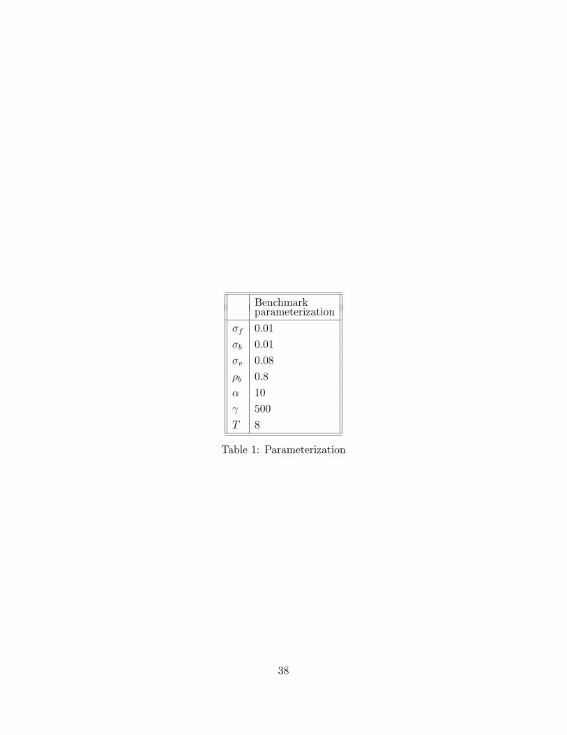
Benchmarkparameterization
�f 0.01
�b 0.01
�v 0.08
�b 0.8
� 10
500
T 8
Table 1: Parameterization
38

Figure 1 Magnification Factor in Model with T=1*
0
4
8
12
16
20
0 0.1 0.2 0.3 0.4 0.5 0.6 0.7 0.8 0.9
Function of σv
Function of σb
σv and σb
*This figure is based on the simulation of the model for T=1, with both bt and ft i.i.d.. The qualitative results do not depend on other model parameters. We set α=10, γ=50, and all standard deviations of the shocks equal to 0.1, unless varied within the Figure.
MagnificationFactor
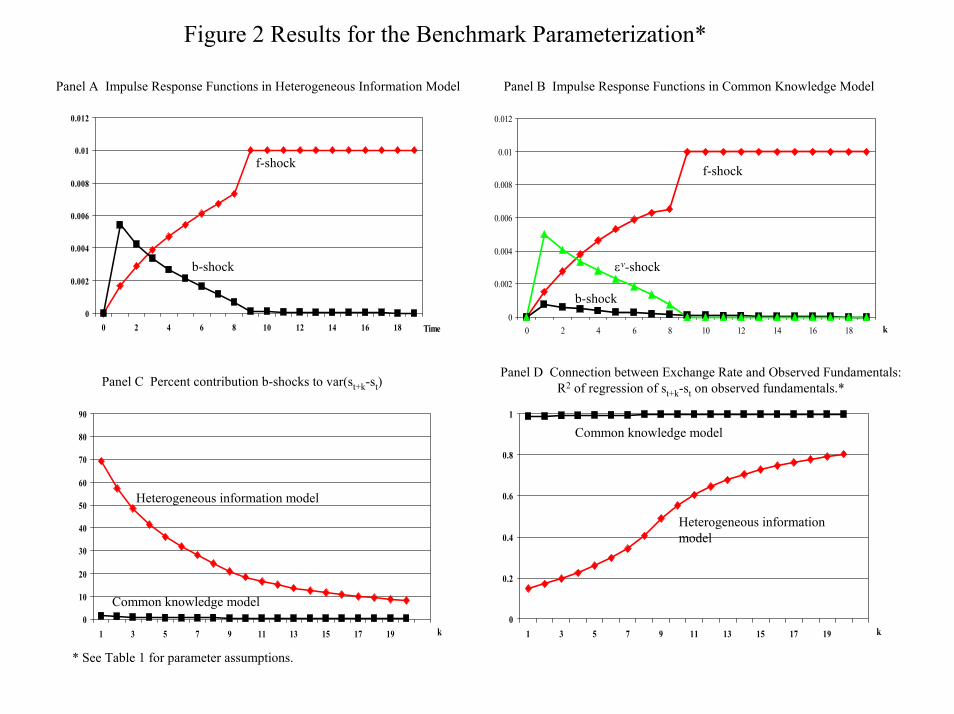
Figure 2 Results for the Benchmark Parameterization*
0
0.002
0.004
0.006
0.008
0.01
0.012
0 2 4 6 8 10 12 14 16 18 Time
Panel A Impulse Response Functions in Heterogeneous Information Model
0
0.002
0.004
0.006
0.008
0.01
0.012
0 2 4 6 8 10 12 14 16 18 k
Panel B Impulse Response Functions in Common Knowledge Model
Panel D Connection between Exchange Rate and Observed Fundamentals: R2 of regression of st+k-st on observed fundamentals.*
0
0.2
0.4
0.6
0.8
1
1 3 5 7 9 11 13 15 17 19 k
* See Table 1 for parameter assumptions.
0
10
20
30
40
50
60
70
80
90
1 3 5 7 9 11 13 15 17 19 k
Panel C Percent contribution b-shocks to var(st+k-st)
f-shock
b-shock
f-shock
εv-shock
b-shock
Heterogeneous information model
Common knowledge model
Heterogeneous information model
Common knowledge model

Figure 2 Results for the Benchmark Parameterization-continued.
0
0.2
0.4
0.6
0.8
1
2 4 6 8 10 12 14 16 18 20 k
Panel E Connection between Exchange Rate and Future Fundamentals:R2 of regression of ft+k-ft+1 on st+1-st.
0.7
0.8
0.9
1
1 3 5 7 9 11 13 15 17 19 21 23 25 27 29 31 33 35 37 39 k
Panel F Connection between Exchange Rate and Order FlowR2 of regression of st+k-st on xt+k-xt.

Figure 3 Four Model Simulations Exchange Rate and Cumulative Order Flow
-0.09
-0.08
-0.07
-0.06
-0.05
-0.04
-0.03
-0.02
-0.01
01 3 5 7 9 11 13 15 17 19 21 23 25 27 29 31 33 35 37 39
Simulation 1
time
Exchange Rate (st)
Cumulative Order Flow (xt)
-0.03
0
0.03
0.06
0.09
0.12
0.15
0.18
1 3 5 7 9 11 13 15 17 19 21 23 25 27 29 31 33 35 37 39
Simulation 2
time
Cumulative Order Flow (xt)
Exchange Rate (st)
-0.04
0
0.04
1 3 5 7 9 11 13 15 17 19 21 23 25 27 29 31 33 35 37 39
Simulation 3
Cumulative Order Flow (xt)
Exchange Rate (st)
time
-0.02
0
0.02
0.04
0.06
1 3 5 7 9 11 13 15 17 19 21 23 25 27 29 31 33 35 37 39
Simulation 4
timeCumulative Order Flow (xt)
Exchange Rate (st)

Figure 4 R2 of regression of st+1-st on (i) observed fundamentals and (ii) order flow:sensitivity analysis.*
0
0 .2
0 .4
0 .6
0 .8
1
0 .0 1 0 .0 3 0 .0 5 0 .0 7 0 .0 9 0 .0 1 0 .0 1 0 .15 0 .17 0 .19 0 .2 10
0 .2
0 .4
0 .6
0 .8
1
0 .0 0 0 0 .0 0 4 0 .0 0 8 0 .0 12 0 .0 16 0 .0 2 0 0 .0 2 4 0 .0 2 8
0
0 .2
0 .4
0 .6
0 .8
1
1.0 0 5 .0 0 9 .0 0 13 .0 0 17 .0 0
σv σb
T
observed fundamentals observed fundamentals
observed fundamentals
order flow order flow
order flow
R2 R2
R2
0
0 .2
0 .4
0 .6
0 .8
1
0 .0 0 0 .2 0 0 .4 0 0 .6 0 0 .8 0 1.0 0
observed fundamentals
order flow
ρb
R2
* Order flow: R2 of regression of st+1-st on xt+1-xt (same as Figure 2F for k=1). Observed fundamentals: R2 of regression st+1-st on all ft+s-ft+s-1 for s²1 (same as Figure 2D for k=1). The figures show how the explanatory power of order flow and observed fundamentals changes when respectively σv,σb, T and ρb are varied, holding constant the other parameters as in the benchmark parameterization.