Boundary matting for view synthesis
Samuel W. Hasinoff Sing Bing Kang Richard Szeliski
Computer Vision and Image Understanding 103 (2006) 22–32
Outline
• Introduction• Method• Result• Conclusion
Introduction
• New view synthesis has emerged as an important application of 3D stereo reconstruction.
• Even if a perfect depth map were available, current methods for view interpolation share two major limitations:
Sampling blurBoundary artifacts
• We propose a method called boundary matting, which represents each occlusion boundary as a 3D curve.

Introduction
• Better suited to view synthesis, because it avoids the blurring associated with resampling those mattes.
• Automatic matting from imperfect stereo data for large-scale opaque objects.
• Exploits information from matting to refine stereo disparities along occlusion boundaries.
• Estimate occlusion boundaries to sub-pixel accuracy, suitable for super-resolution or zooming.
• Error metric is symmetric with respect to the input images.

Method• To model the matting effects at occlusion boundaries, we use
the well-known compositing equation
• The triangulation method operates by observing foreground objects in front of V known backgrounds giving the linear system
• The 3D subpixel boundary curves lead to different alpha’s across viewpoint in general.

Method
• Assume the occluding contours of the foreground objects are sufficiently sharp relative to both the closeness of the views and the standoff distance of the cameras.
• The 3D curve as a spline parameterized by control points, .
• In the ideal case, with a Dirac point spread function, the continuous alpha matte for the i-th view is

• Simulate image blurring due to camera optics and motion by convolving a with an isotropic 2D Gaussian function :
• Objective function


Method
• The starting point for boundary matting is an initialization derived from stereo and the attendant camera calibration.
• This method computes stereo by combining shiftable windows for matching with global minimization using graph cuts for visibility reasoning.
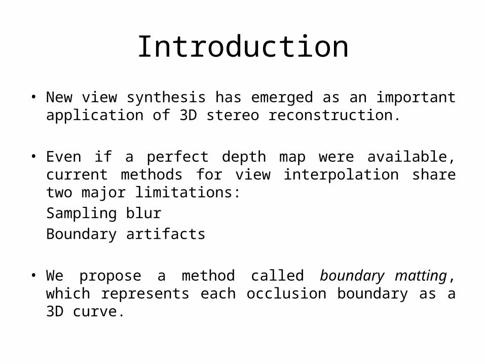
• To extract the initial curves h0 corresponding to occlusion boundaries, we first form a depth discontinuity map by applying a manually selected threshold to the gradient of the disparity map for the reference view.

Background (clean plate) estimation
• For a given boundary pixel, we find potentially corresponding background colors by forward-warping that pixel to all other views.
• We use a color inconsistency measure to select the corresponding background pixel most likely to consist of pure background color.
• For each candidate background pixel, we compute its ‘‘color inconsistency’’ as the maximum L2 distance in RGB space between its color and any of its eight-neighbors that are also labeled at background depth.
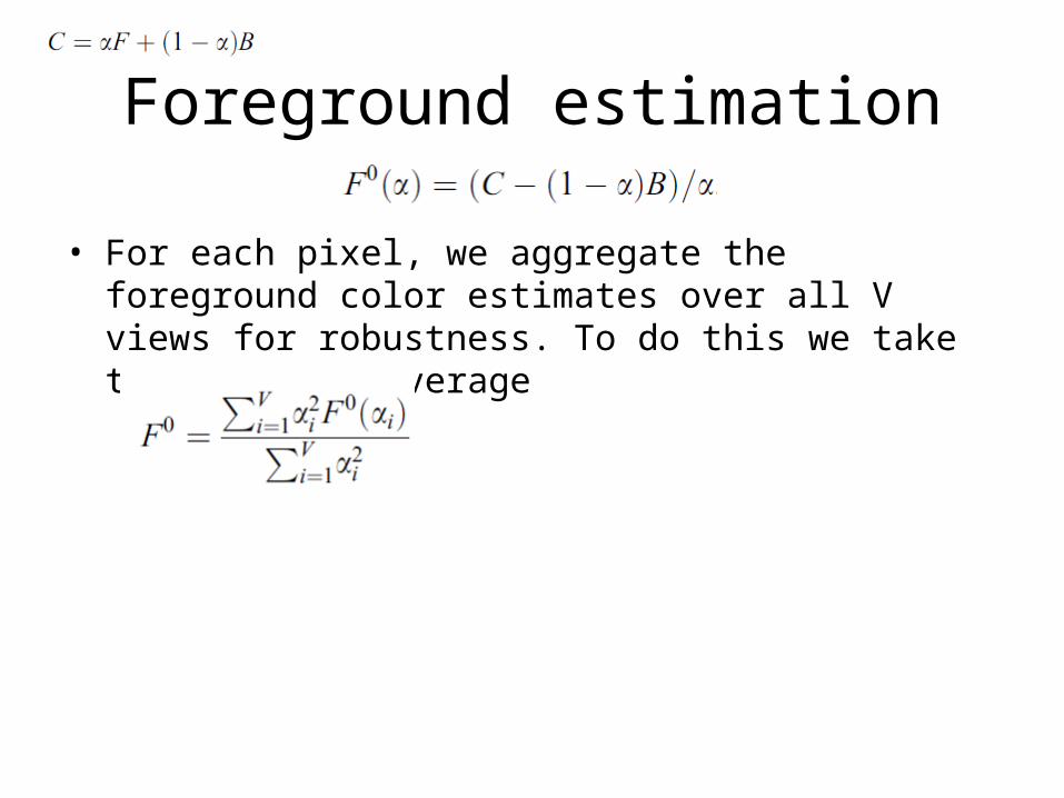
Foreground estimation
• For each pixel, we aggregate the foreground color estimates over all V views for robustness. To do this we take the weighted average

Result
• For all datasets, we used five input views, with the middle view designated as the reference view for initialization.
• A typical run for a 300-pixel boundary in five views could take approximately five minutes to complete, converging within 20 iterations

Result
344*240 640*486 434*380


Result
Result

Conclusion
• For seamless view interpolation, mixed boundary pixels must be resolved into foreground and background components. Boundary matting appears to be a useful tool for addressing this problem in an automatic way.
• Using 3D curves to model occlusion boundaries is a natural representation that provides several benefits, including the ability to super-resolve the depth maps near occlusion boundaries.