Binary Contingency Tables in Theory and Practice
Ivona Bezáková(Rochester Institute of Technology)
Based on joint works with Nayantara Bhatnagar, Alistair Sinclair, Daniel Štefankovič, and Eric Vigoda.
DIMACS Workshop on Markov Chain Monte Carlo: Synthesizing Theory and Practice June 5th, 2007

The Voyage of the Beagle
Galápagos archipelago (1835)
Darwin’s Finches

© Robert H. Rothman
Darwin’s Finches
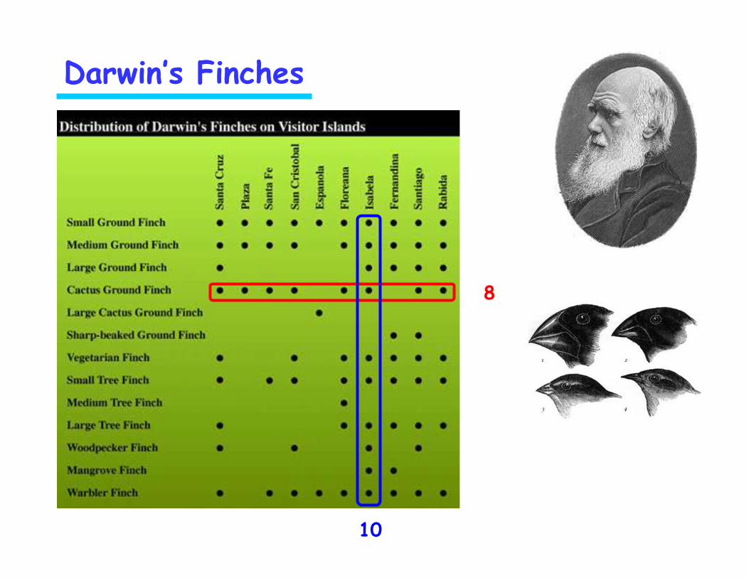
10
8
Darwin’s Finches

Darwin’s Finches
8
96
2378164210
10
9 3 5 7 3 8 10 9 10 8
chance
OR
competitive pressures
?

Input:
Sample space: 0/1 tables satisfying the marginals
Goal: count / sample
2
3
21
3
32
5
3 4 2
4
Binary Contingency Tables
marginals(row sums r1, r2, …, rm, column sums c1, c2, …, cn)

Input:
Sample space: 0/1 tables satisfying the marginals
Goal: count / sample
Binary Contingency Tables
marginals(row sums r1, r2, …, rm, column sums c1, c2, …, cn)
2
3
21
3
32
5
3 4 2
41111
11
111
1111 1
1 11

Different Approaches
Theory (Markov chain Monte Carlo with simulated annealing)
• Jerrum-Sinclair-Vigoda ’01: approximate permanent in O*(n10), yields O*((mn)10) algorithm for m x n binary contingency tables
• Bezáková-Bhatnagar-Vigoda ’06: O*((mn)3(m+n)5)
Practice (sequential importance sampling, Chen-Diaconis-Holmes-Liu ’05)
• Bezáková-Sinclair-Štefankovič-Vigoda ’06: negative example
• Jose Blanchet ’06: SIS works if marginals O(n1/4)
• Bayati-Kim-Saberi ’07: alternative importance sampling method, works if marginals O(n1/4)
Practice (the switching Markov chain, Diaconis-Gangolli ’94)
• Kannan-Tetali-Vempala ’97, Cooper-Dyer-Greenhill ’05: works for regular marginals

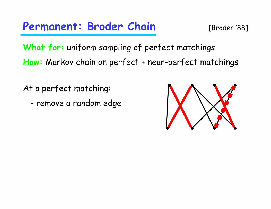
Permanent: Broder Chain [Broder ’88]
What for: uniform sampling of perfect matchings
How: Markov chain on perfect + near-perfect matchings
Perfect matching:
Permanent:
subset of vertex-disjoint edges covering all vertices
number of all perfect matchings

What for: uniform sampling of perfect matchings
How: Markov chain on perfect + near-perfect matchings
Permanent: Broder Chain [Broder ’88]
Perfect matching:
Permanent:
subset of vertex-disjoint edges covering all vertices
number of all perfect matchings

At a perfect matching:
- remove a random edge
What for: uniform sampling of perfect matchings
How: Markov chain on perfect + near-perfect matchings
Permanent: Broder Chain [Broder ’88]
At a perfect matching:
- remove a random edge
What for: uniform sampling of perfect matchings
How: Markov chain on perfect + near-perfect matchings
Permanent: Broder Chain [Broder ’88]

At a perfect matching:
- remove a random edge
What for: uniform sampling of perfect matchings
How: Markov chain on perfect + near-perfect matchings
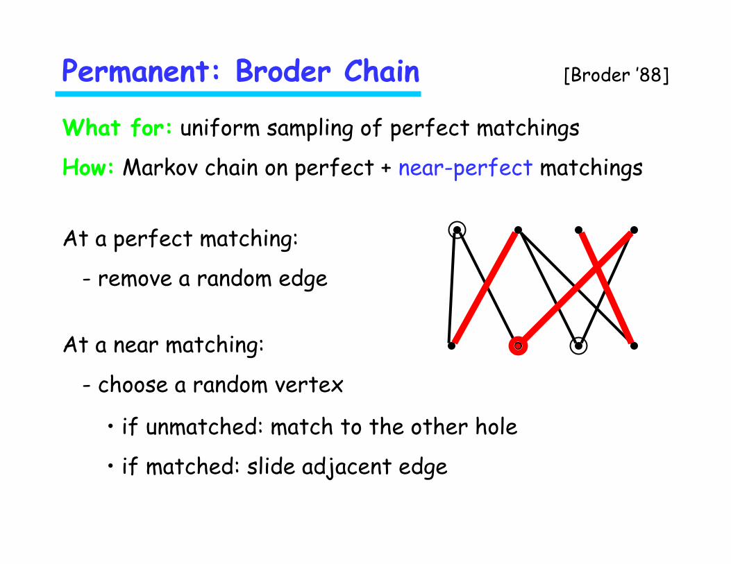
Permanent: Broder Chain [Broder ’88]

At a perfect matching:
- remove a random edge
At a near matching:
- choose a random vertex
What for: uniform sampling of perfect matchings
How: Markov chain on perfect + near-perfect matchings
Permanent: Broder Chain [Broder ’88]

At a perfect matching:
- remove a random edge
At a near matching:
- choose a random vertex
• if unmatched: match to the other hole
What for: uniform sampling of perfect matchings
How: Markov chain on perfect + near-perfect matchings
Permanent: Broder Chain [Broder ’88]

At a perfect matching:
- remove a random edge
At a near matching:
- choose a random vertex
• if unmatched: match to the other hole
What for: uniform sampling of perfect matchings
How: Markov chain on perfect + near-perfect matchings
Permanent: Broder Chain [Broder ’88]

At a perfect matching:
- remove a random edge
At a near matching:
- choose a random vertex
• if unmatched: match to the other hole
What for: uniform sampling of perfect matchings
How: Markov chain on perfect + near-perfect matchings
Permanent: Broder Chain [Broder ’88]

At a perfect matching:
- remove a random edge
At a near matching:
- choose a random vertex
• if unmatched: match to the other hole
What for: uniform sampling of perfect matchings
How: Markov chain on perfect + near-perfect matchings
Permanent: Broder Chain [Broder ’88]

At a perfect matching:
- remove a random edge
At a near matching:
- choose a random vertex
What for: uniform sampling of perfect matchings
How: Markov chain on perfect + near-perfect matchings
• if unmatched: match to the other hole
• if matched: slide adjacent edge
Permanent: Broder Chain [Broder ’88]
At a perfect matching:
- remove a random edge
At a near matching:
- choose a random vertex
• if unmatched: match to the other hole
• if matched: slide adjacent edge
What for: uniform sampling of perfect matchings
How: Markov chain on perfect + near-perfect matchings
Permanent: Broder Chain [Broder ’88]

Broder Chain
Mixes in polynomial time ? Even if it did…

Broder Chain
Mixes in polynomial time ? Even if it did…
1 perfect matching

Broder Chain
Mixes in polynomial time ? Even if it did…
1 perfect matching
near matchings≥2(n/4)

Broder Chain
Mixes in polynomial time ? Even if it did…
1 perfect matching
near matchings≥2(n/4)
Thm [Jerrum-Sinclair ’89]:Rapid mixing if perfects polynomially related to nears.

Jerrum-Sinclair-Vigoda ’01:Change the weight so that perfect matchingstake polynomial fraction.
Simulated Annealing for Permanent
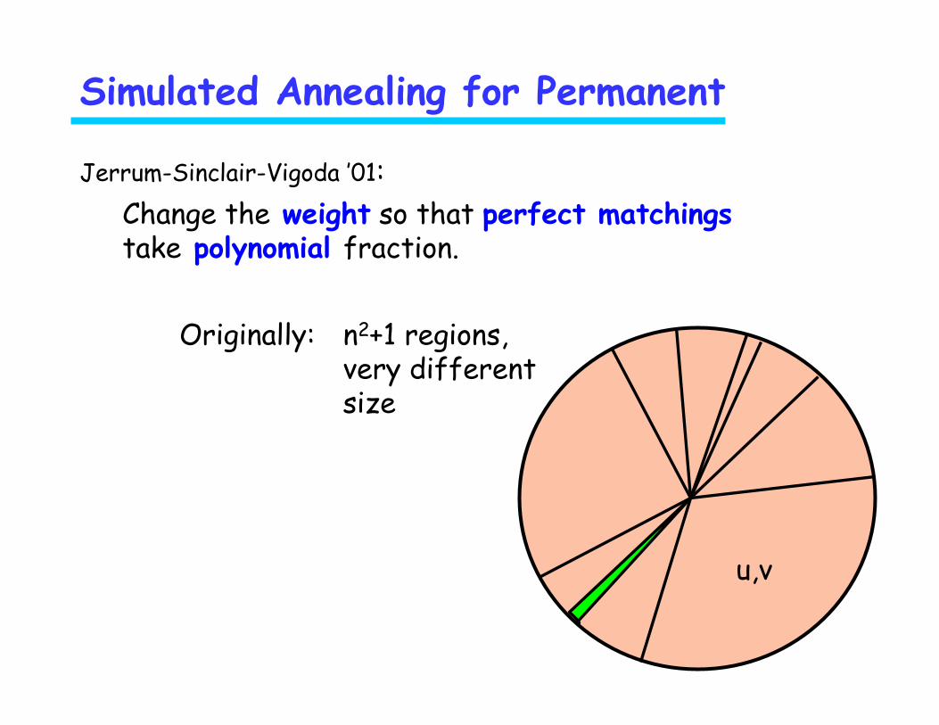
Jerrum-Sinclair-Vigoda ’01:
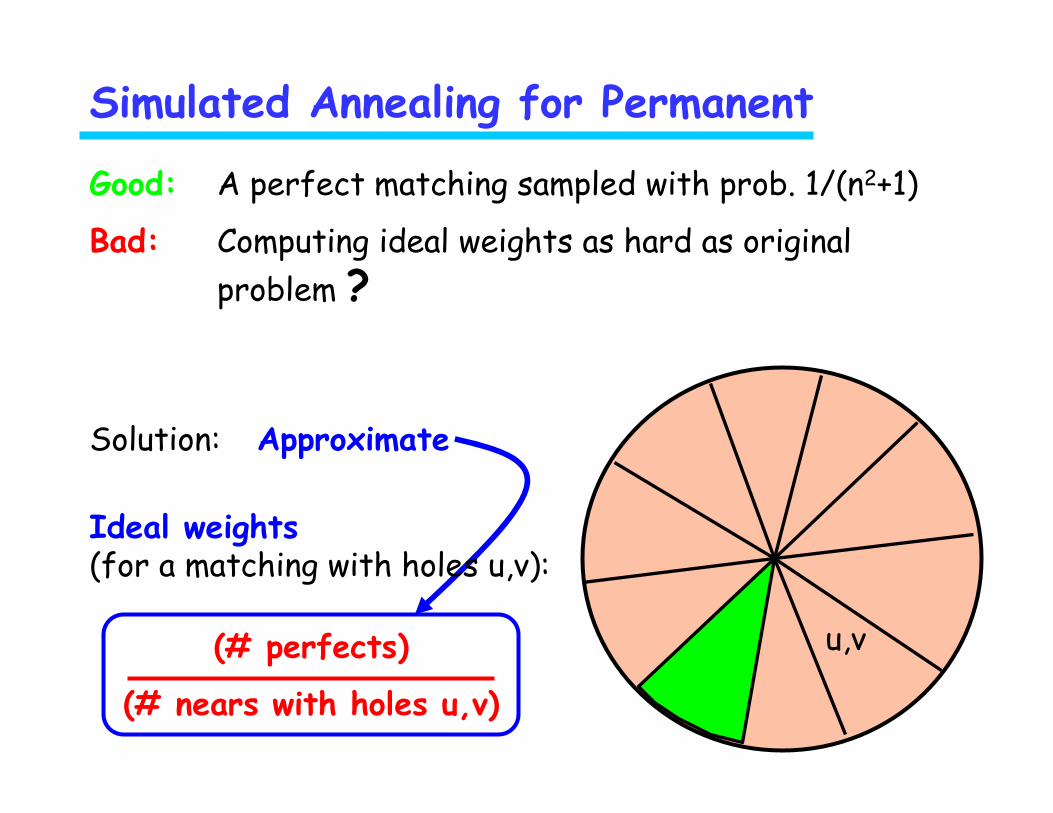
n2+1 regions, very different size
u,v
Change the weight so that perfect matchingstake polynomial fraction.
Originally:
Simulated Annealing for Permanent

Jerrum-Sinclair-Vigoda ’01:
n2+1 regions, very different size
u,v
the same
Change the weight so that perfect matchingstake polynomial fraction.
Want:
Simulated Annealing for Permanent

Jerrum-Sinclair-Vigoda ’01:
u,v
Ideal weights(for a matching with holes u,v):
(# perfects)
(# nears with holes u,v)
n2+1 regions, very different sizethe same
Change the weight so that perfect matchingstake polynomial fraction.
Simulated Annealing for Permanent
Want:
u,v
Ideal weights(for a matching with holes u,v):
(# perfects)
(# nears with holes u,v)
A perfect matching sampled with prob. 1/(n2+1)
Computing ideal weights as hard as original problem ?
Good:
Bad:
Solution: Approximate
Simulated Annealing for Permanent

Simulated Annealing for Permanent
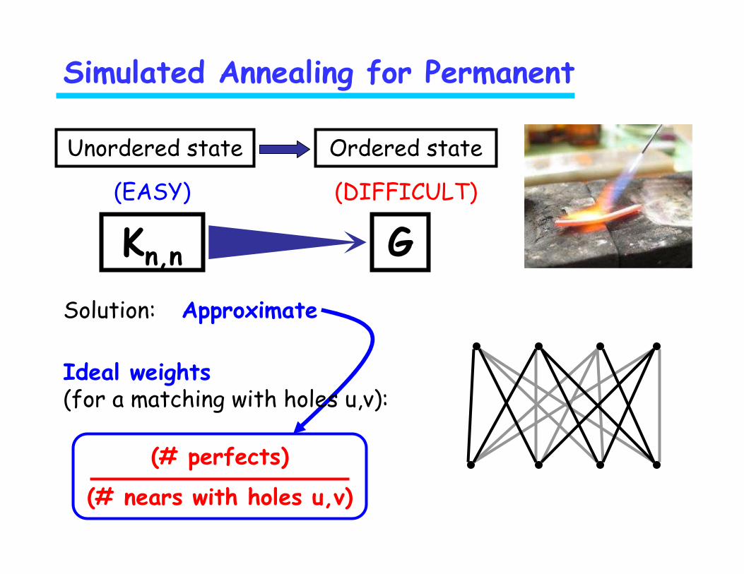
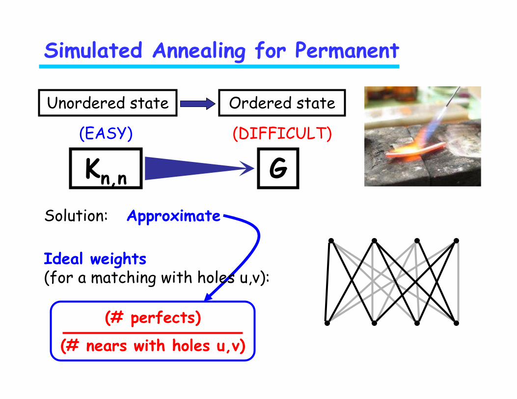
Ideal weights(for a matching with holes u,v):
(# perfects)
(# nears with holes u,v)
Unordered state Ordered state
(EASY) (DIFFICULT)
Solution: Approximate
G
G

Simulated Annealing for Permanent
Ideal weights(for a matching with holes u,v):
(# perfects)
(# nears with holes u,v)
Kn,n G
Unordered state Ordered state
(EASY) (DIFFICULT)
Solution: Approximate
Kn,n

Simulated Annealing for Permanent
Ideal weights(for a matching with holes u,v):
(# perfects)
(# nears with holes u,v)
Kn,n G
Unordered state Ordered state
(EASY) (DIFFICULT)
Solution: Approximate

Simulated Annealing for Permanent
Ideal weights(for a matching with holes u,v):
(# perfects)
(# nears with holes u,v)
Kn,n G
Unordered state Ordered state
(EASY) (DIFFICULT)
Solution: Approximate

Simulated Annealing for Permanent
Ideal weights(for a matching with holes u,v):
(# perfects)
(# nears with holes u,v)
Kn,n G
Unordered state Ordered state
(EASY) (DIFFICULT)
Solution: Approximate
Simulated Annealing for Permanent
Ideal weights(for a matching with holes u,v):
(# perfects)
(# nears with holes u,v)
Kn,n G
Unordered state Ordered state
(EASY) (DIFFICULT)
Solution: Approximate
Simulated Annealing for Permanent
Ideal weights(for a matching with holes u,v):
(# perfects)
(# nears with holes u,v)
Kn,n G
Unordered state Ordered state
(EASY) (DIFFICULT)
Solution: Approximate

Simulated Annealing for Permanent
Ideal weights(for a matching with holes u,v):
(# perfects)
(# nears with holes u,v)
Kn,n G
Unordered state Ordered state
(EASY) (DIFFICULT)
Solution: Approximate

Simulated Annealing for Permanent
Ideal weights(for a matching with holes u,v):
(# perfects)
(# nears with holes u,v)
Kn,n G
Unordered state Ordered state
(EASY) (DIFFICULT)
Solution: Approximate

Simulated Annealing for Permanent
Ideal weights(for a matching with holes u,v):
(# perfects)
(# nears with holes u,v)
Kn,n G
Unordered state Ordered state
(EASY) (DIFFICULT)
Solution: Approximate

Simulated Annealing for Permanent
Ideal weights(for a matching with holes u,v):
(# perfects)
(# nears with holes u,v)
Kn,n G
Unordered state Ordered state
(EASY) (DIFFICULT)
Solution: Approximate
G

Simulated Annealing for Permanent
Ideal weights(for a matching with holes u,v):
(# perfects)
(# nears with holes u,v)
Kn,n G
Unordered state Ordered state
(EASY) (DIFFICULT)
Solution: Approximate λλλλ = 1 … ~0
1

Simulated Annealing for Permanent
Ideal weights(# perfects)
(# nears with holes u,v)
λλλλ = 1 … ~0
1
need to be λλλλ-weighted:
w(u,v) =
λλλλ(M) = λλλλ# λλλλ-edges in M
λλλλ(S) = ∑∑∑∑ λλλλ(M)
where
λλλλ( P P P P )
λλλλ( N N N N (u,v) )
M in S

Simulated Annealing for Permanent
λλλλ = 1
1
λλλλ( P P P P )
λλλλ( N N N N (u,v) )w(u,v) =
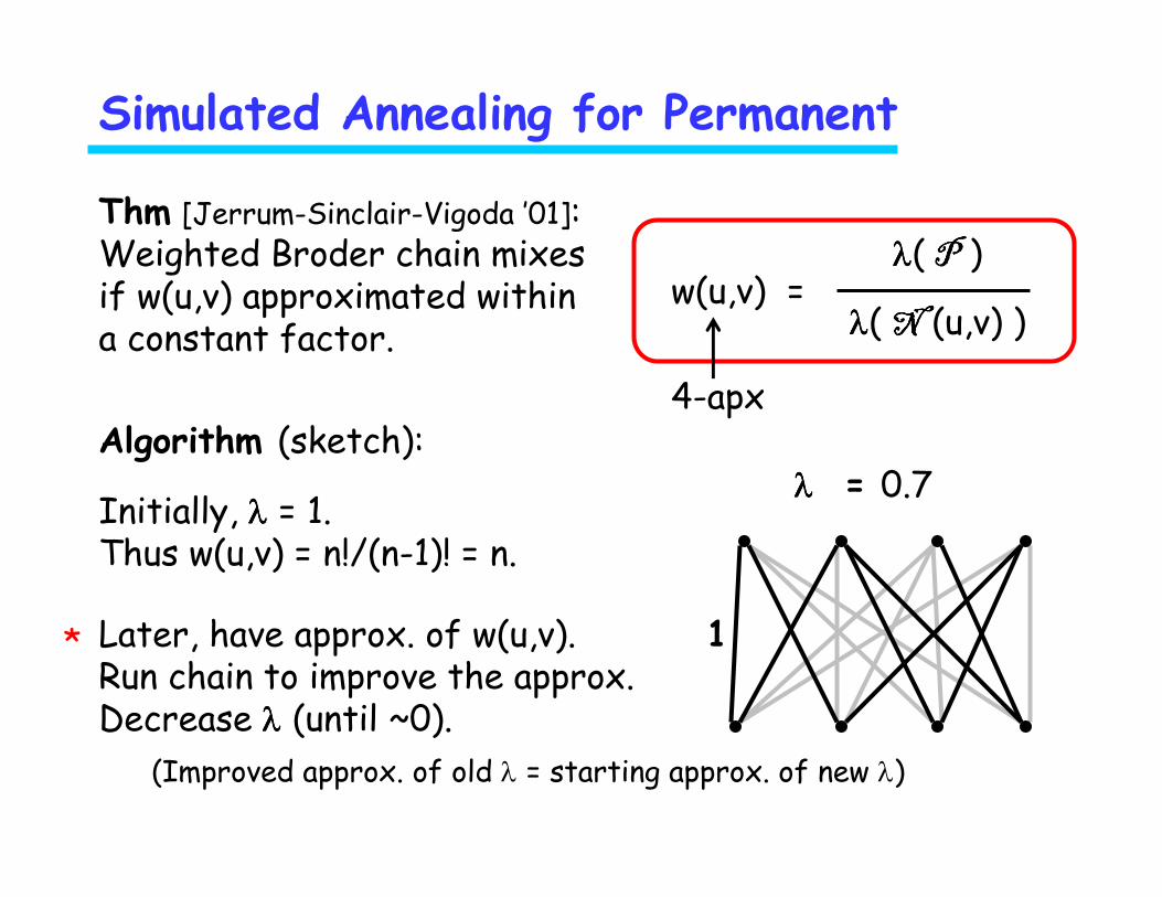
Initially, λλλλ = 1. Thus w(u,v) = n!/(n-1)! = n.
Algorithm (sketch):
Later, have approx. of w(u,v). Run chain to improve the approx. Decrease λλλλ (until ~0).
(Improved approx. of old λ = starting approx. of new λ)
*
Thm [Jerrum-Sinclair-Vigoda ’01]: Weighted Broder chain mixes if w(u,v) approximated within a constant factor.
Simulated Annealing for Permanent
λλλλ = 0.7
1
λλλλ( P P P P )
λλλλ( N N N N (u,v) )w(u,v) =
Initially, λλλλ = 1. Thus w(u,v) = n!/(n-1)! = n.
Algorithm (sketch):
Later, have approx. of w(u,v). Run chain to improve the approx. Decrease λλλλ (until ~0).
(Improved approx. of old λ = starting approx. of new λ)
4-apx
*
Thm [Jerrum-Sinclair-Vigoda ’01]: Weighted Broder chain mixes if w(u,v) approximated within a constant factor.

Simulated Annealing for Permanent
λλλλ = 0.7
1
λλλλ( P P P P )
λλλλ( N N N N (u,v) )w(u,v) =
Initially, λλλλ = 1. Thus w(u,v) = n!/(n-1)! = n.
Thm [Jerrum-Sinclair-Vigoda ’01]: Weighted Broder chain mixes if w(u,v) approximated within a constant factor.
Algorithm (sketch):
Later, have approx. of w(u,v). Run chain to improve the approx. Decrease λλλλ (until ~0).
(Improved approx. of old λ = starting approx. of new λ)
4-apx2
*

Simulated Annealing for Permanent
λλλλ = 0.7 0.6
1
λλλλ( P P P P )
λλλλ( N N N N (u,v) )w(u,v) =
Initially, λλλλ = 1. Thus w(u,v) = n!/(n-1)! = n.
Algorithm (sketch):
Later, have approx. of w(u,v). Run chain to improve the approx. Decrease λλλλ (until ~0).
(Improved approx. of old λ = starting approx. of new λ)
4-apx2 = 4-apx for
*
Thm [Jerrum-Sinclair-Vigoda ’01]: Weighted Broder chain mixes if w(u,v) approximated within a constant factor.

Simulated Annealing for Permanent
λλλλ = 0.7 0.6 …~0
1
λλλλ( P P P P )
λλλλ( N N N N (u,v) )w(u,v) =
Initially, λλλλ = 1. Thus w(u,v) = n!/(n-1)! = n.
Algorithm (sketch):
Later, have approx. of w(u,v). Run chain to improve the approx. Decrease λλλλ (until ~0).
(Improved approx. of old λ = starting approx. of new λ)
4-apx2 = 4-apx for
*
Thm [Jerrum-Sinclair-Vigoda ’01]: Weighted Broder chain mixes if w(u,v) approximated within a constant factor.

0 1 0 1
1 1 0 0
1 0 1 0
0 1 0 1
columns
rows
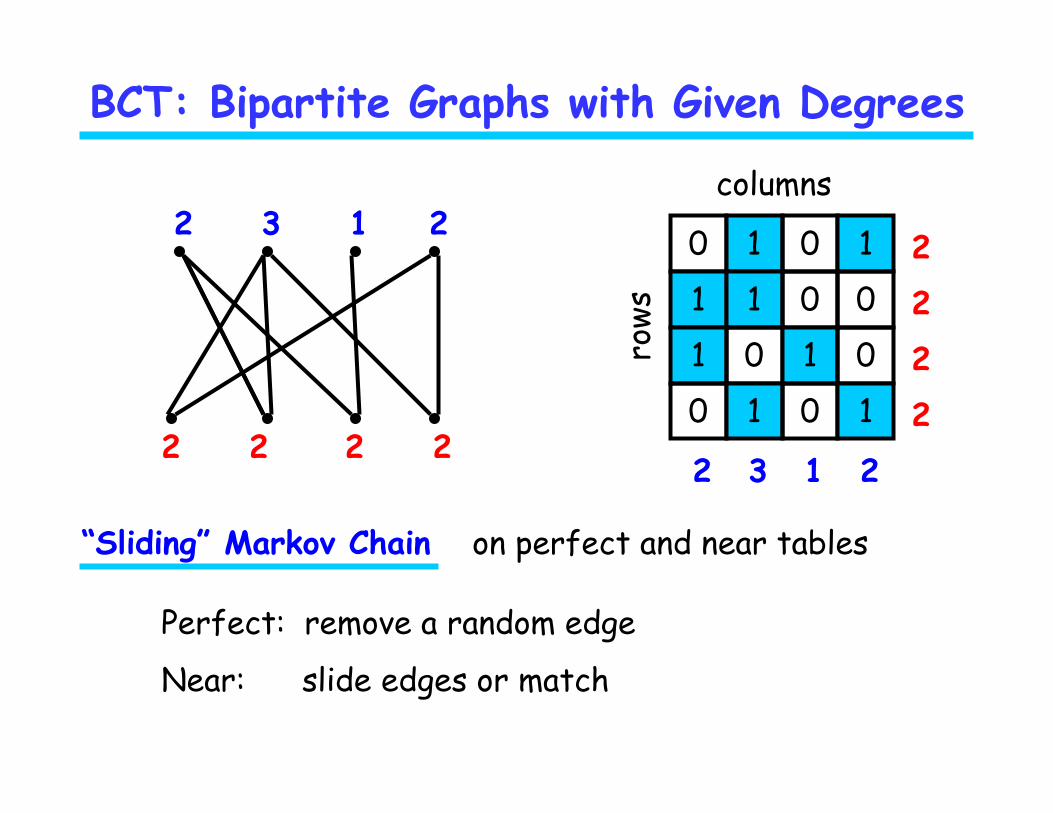
BCT: Bipartite Graphs with Given Degrees
2
2
2
2
2 3 1 2
2 3 1 2
2 2 2 2
columns
rows
0 1 0 1
1 1 0 0
1 0 1 0
0 1 0 1
columns
rows
BCT: Bipartite Graphs with Given Degrees
2
2
2
2
2 3 1 2
2 3 1 2
2 2 2 2
“Sliding” Markov Chain on perfect and near tables
Perfect: remove a random edge
Near: slide edges or match

0 1 0 1
1 1 0 0
1 0 1 0
0 1 0 1
columns
rows
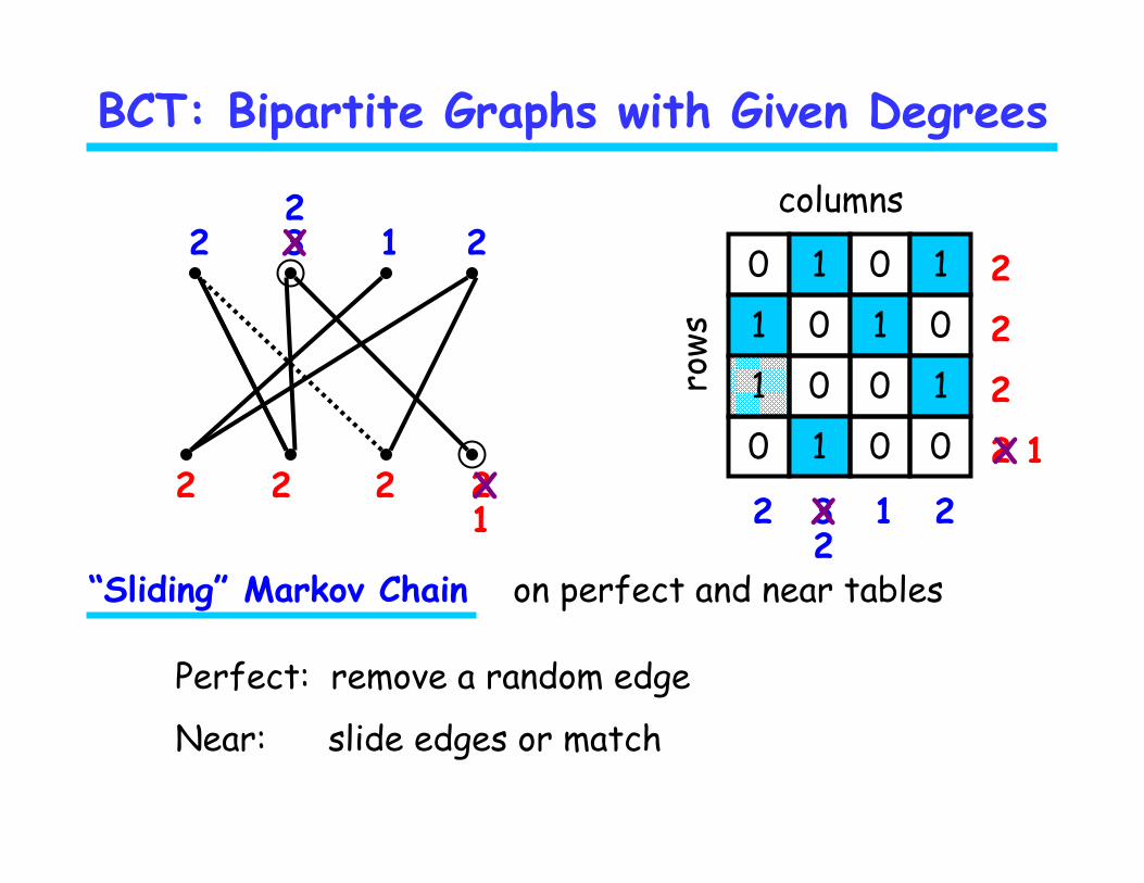
BCT: Bipartite Graphs with Given Degrees
2
2
2
2
2 3 1 2
2 3 1 2
2 2 2 2
“Sliding” Markov Chain on perfect and near tables
Perfect: remove a random edge
Near: slide edges or match

2 0 1 0 1
1 1 0 0
1 0 1 0
0 1 0 0
columns
rows
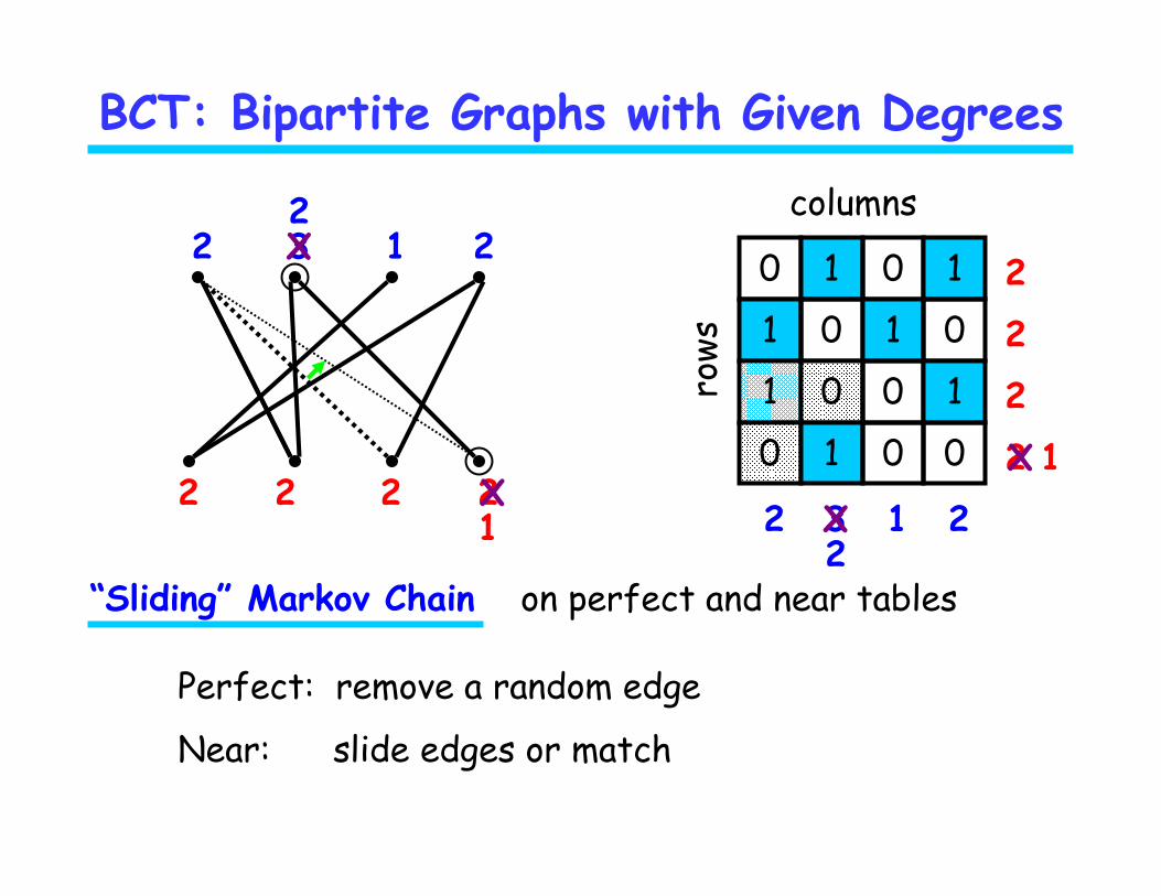
BCT: Bipartite Graphs with Given Degrees
2
2
2
2
2 3 1 2
2 3 1
2 2 2 2
“Sliding” Markov Chain on perfect and near tables
Perfect: remove a random edge
Near: slide edges or match
1
1
X
XX
X
1
1

2 0 1 0 1
1 1 0 0
1 0 1 0
0 1 0 0
columns
rows
BCT: Bipartite Graphs with Given Degrees
2
2
2
2
2 3 1 2
2 3 1
2 2 2 2
“Sliding” Markov Chain on perfect and near tables
Perfect: remove a random edge
Near: slide edges or match
1
1
X
XX
X
1
1

2 0 1 0 1
1 1 0 0
1 0 1 0
0 1 0 0
columns
rows
BCT: Bipartite Graphs with Given Degrees
2
2
2
2
2 3 1 2
2 3 1
2 2 2 2
“Sliding” Markov Chain on perfect and near tables
Perfect: remove a random edge
Near: slide edges or match
1
1
X
XX
X
1
1

2 0 1 0 1
1 1 0 0
1 0 1 0
0 1 0 0
columns
rows
BCT: Bipartite Graphs with Given Degrees
2
2
2
2
2 3 1 2
2 3 1
2 2 2 2
“Sliding” Markov Chain on perfect and near tables
Perfect: remove a random edge
Near: slide edges or match
1
1
X
XX
X
1
1

2 0 1 0 1
1 1 0 0
1 0 0 1
0 1 0 0
columns
rows
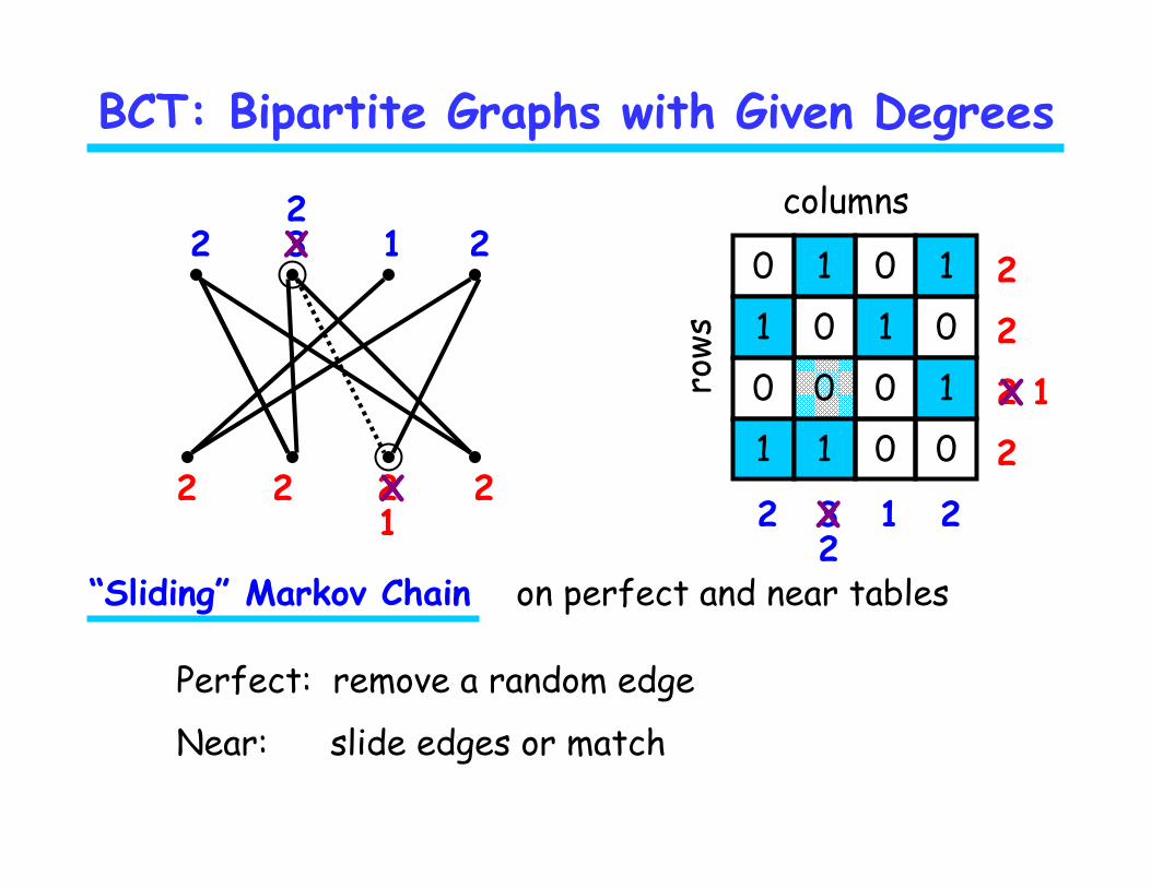
BCT: Bipartite Graphs with Given Degrees
2
2
2
2
2 3 1 2
2 3 1
2 2 2 2
“Sliding” Markov Chain on perfect and near tables
Perfect: remove a random edge
Near: slide edges or match
0
1
X
XX
X
1
0

2 0 1 0 1
1 1 0 0
1 0 0 1
0 1 0 0
columns
rows
BCT: Bipartite Graphs with Given Degrees
2
2
2
2
2 3 1 2
2 3 1
2 2 2 2
“Sliding” Markov Chain on perfect and near tables
Perfect: remove a random edge
Near: slide edges or match
0
1
X
XX
X
1
0

2 0 1 0 1
1 1 0 0
1 0 0 1
0 1 0 0
columns
rows
BCT: Bipartite Graphs with Given Degrees
2
2
2
2
2 3 1 2
2 3 1
2 2 2 2
“Sliding” Markov Chain on perfect and near tables
Perfect: remove a random edge
Near: slide edges or match
0
1
X
XX
X
1
0

2 0 1 0 1
1 0 1 0
1 0 0 1
0 1 0 0
columns
rows
BCT: Bipartite Graphs with Given Degrees
2
2
2
2
2 3 1 2
2 3 1
2 2 2 2
“Sliding” Markov Chain on perfect and near tables
Perfect: remove a random edge
Near: slide edges or match
2
1
X
XX
X
1
2
2 0 1 0 1
1 0 1 0
1 0 0 1
0 1 0 0
columns
rows
BCT: Bipartite Graphs with Given Degrees
2
2
2
2
2 3 1 2
2 3 1
2 2 2 2
“Sliding” Markov Chain on perfect and near tables
Perfect: remove a random edge
Near: slide edges or match
2
1
X
XX
X
1
2

2 0 1 0 1
1 0 1 0
1 0 0 1
0 1 0 0
columns
rows
BCT: Bipartite Graphs with Given Degrees
2
2
2
2
2 3 1 2
2 3 1
2 2 2 2
“Sliding” Markov Chain on perfect and near tables
Perfect: remove a random edge
Near: slide edges or match
2
1
X
XX
X
1
2
2 0 1 0 1
1 0 1 0
1 0 0 1
0 1 0 0
columns
rows
BCT: Bipartite Graphs with Given Degrees
2
2
2
2
2 3 1 2
2 3 1
2 2 2 2
“Sliding” Markov Chain on perfect and near tables
Perfect: remove a random edge
Near: slide edges or match
2
1
X
XX
X
1
2

2 0 1 0 1
1 0 1 0
0 0 0 1
1 1 0 0
columns
rows
BCT: Bipartite Graphs with Given Degrees
2
2
2
2
2 3 1 2
2 3 1
2 2 2 2
“Sliding” Markov Chain on perfect and near tables
Perfect: remove a random edge
Near: slide edges or match
2
1
X
X
X
X
1
2
2 0 1 0 1
1 0 1 0
0 0 0 1
1 1 0 0
columns
rows
BCT: Bipartite Graphs with Given Degrees
2
2
2
2
2 3 1 2
2 3 1
2 2 2 2
“Sliding” Markov Chain on perfect and near tables
Perfect: remove a random edge
Near: slide edges or match
2
1
X
X
X
X
1
2

2 0 1 0 1
1 0 1 0
0 1 0 1
1 1 0 0
columns
rows
BCT: Bipartite Graphs with Given Degrees
2
2
2
2
2 3 1 2
2 3 1
2 2 2 2
“Sliding” Markov Chain on perfect and near tables
Perfect: remove a random edge
Near: slide edges or match

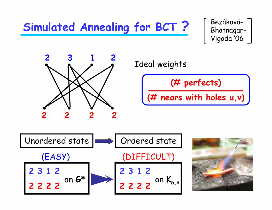
Simulated Annealing for BCT ?
22 3 1
2 2 2 2
Ideal weights
(# perfects)
(# nears with holes u,v)
Unordered state Ordered state
(EASY) (DIFFICULT)
2 3 1 2
2 2 2 2?
Bezáková-Bhatnagar-Vigoda ’06

Simulated Annealing for BCT ?
22 3 1
2 2 2 2
Ideal weights
(# perfects)
(# nears with holes u,v)
Unordered state Ordered state
(EASY) (DIFFICULT)
2 3 1 2
2 2 2 2? on Kn,n
Bezáková-Bhatnagar-Vigoda ’06
Simulated Annealing for BCT ?
22 3 1
2 2 2 2
Ideal weights
(# perfects)
(# nears with holes u,v)
Unordered state Ordered state
(EASY) (DIFFICULT)
2 3 1 2
2 2 2 2on Kn,n
2 3 1 2
2 2 2 2on G*
Bezáková-Bhatnagar-Vigoda ’06

Simulated Annealing for BCT ?
22 3 1
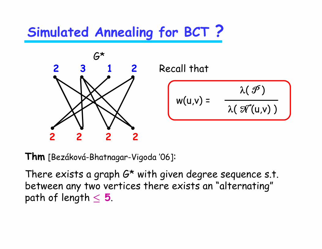
2 2 2 2 where
w(u,v) = λλλλ( P P P P )
λλλλ( N N N N (u,v) )
T in S
λλλλ(T) = λλλλ# λλλλ-edges in T
λλλλ(S) = ∑∑∑∑ λλλλ(T)
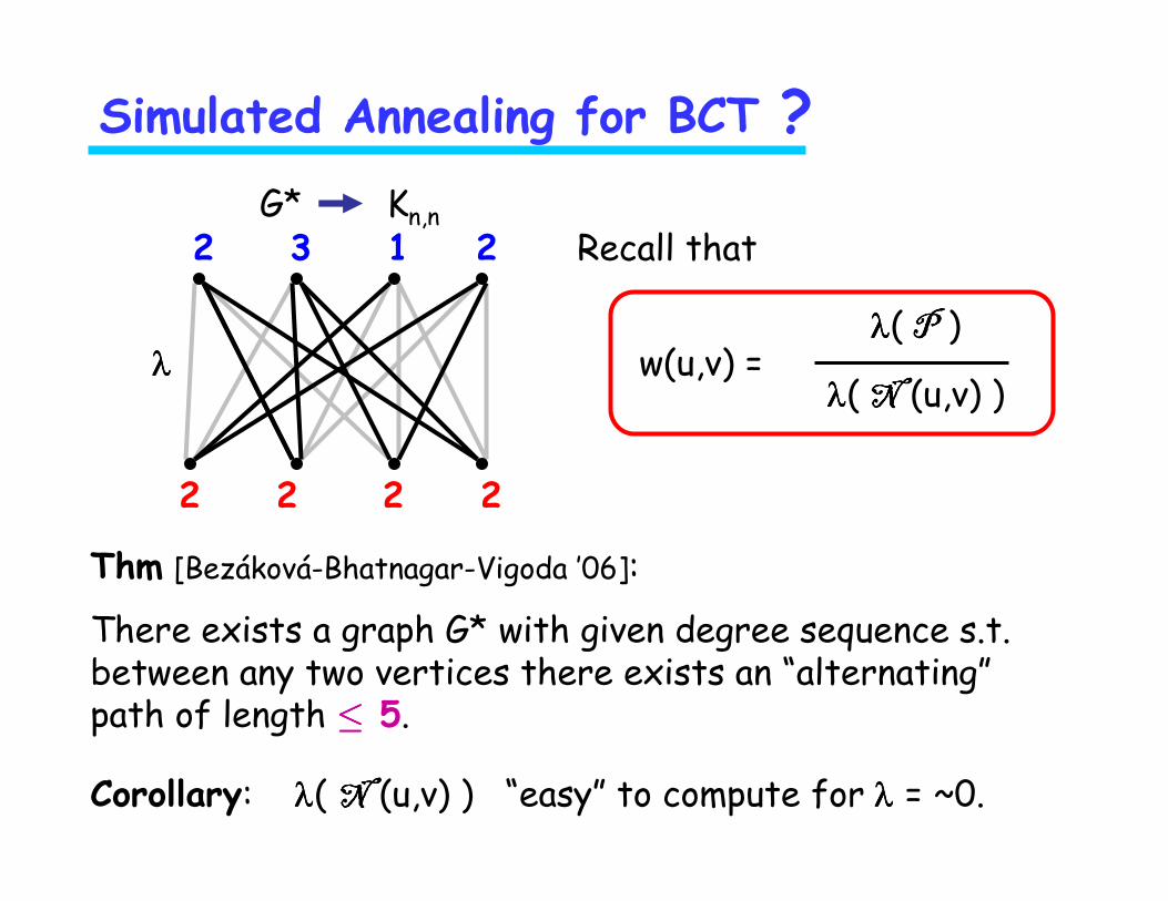
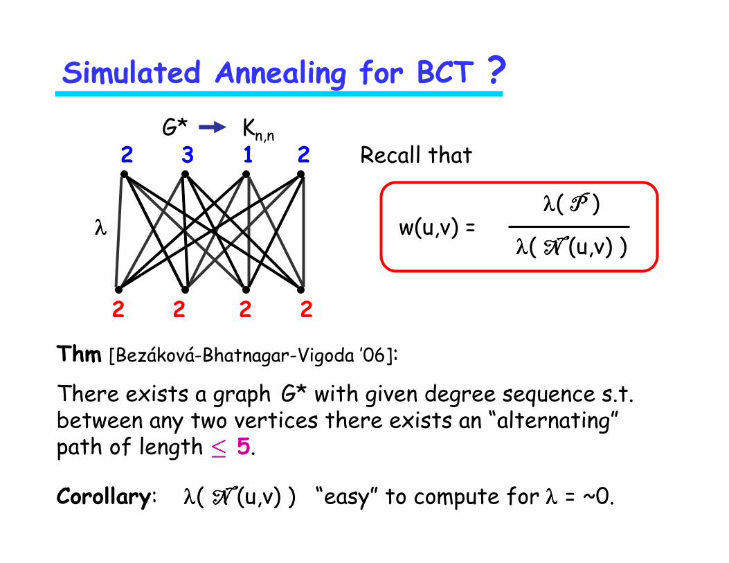
Recall that
2 3 1 2
2 2 2 2on Kn,n
2 3 1 2
2 2 2 2on G*
λλλλ = ~0
λλλλ
……………………… 1

Simulated Annealing for BCT ?
22 3 1
2 2 2 2
λλλλ
The catch :
What, if for some u,v, there is no near-table which uses all real edges ? Then,
λλλλ( N N N N (u,v) ) = 0 for λλλλ = 0.
where
w(u,v) = λλλλ( P P P P )
λλλλ( N N N N (u,v) )
T in S
λλλλ(T) = λλλλ# λλλλ-edges in T
λλλλ(S) = ∑∑∑∑ λλλλ(T)
Recall that
Simulated Annealing for BCT ?
22 3 1
2 2 2 2
w(u,v) = λλλλ( P P P P )
λλλλ( N N N N (u,v) )
Recall that
Thm [Bezáková-Bhatnagar-Vigoda ’06]:
There exists a graph G* with given degree sequence s.t. between any two vertices there exists an “alternating”path of length ≤≤≤≤ 5.
G*

Simulated Annealing for BCT ?
22 3 1
2 2 2 2
w(u,v) = λλλλ( P P P P )
λλλλ( N N N N (u,v) )
Recall that
Thm [Bezáková-Bhatnagar-Vigoda ’06]:
There exists a graph G* with given degree sequence s.t. between any two vertices there exists an “alternating”path of length ≤≤≤≤ 5.
G*
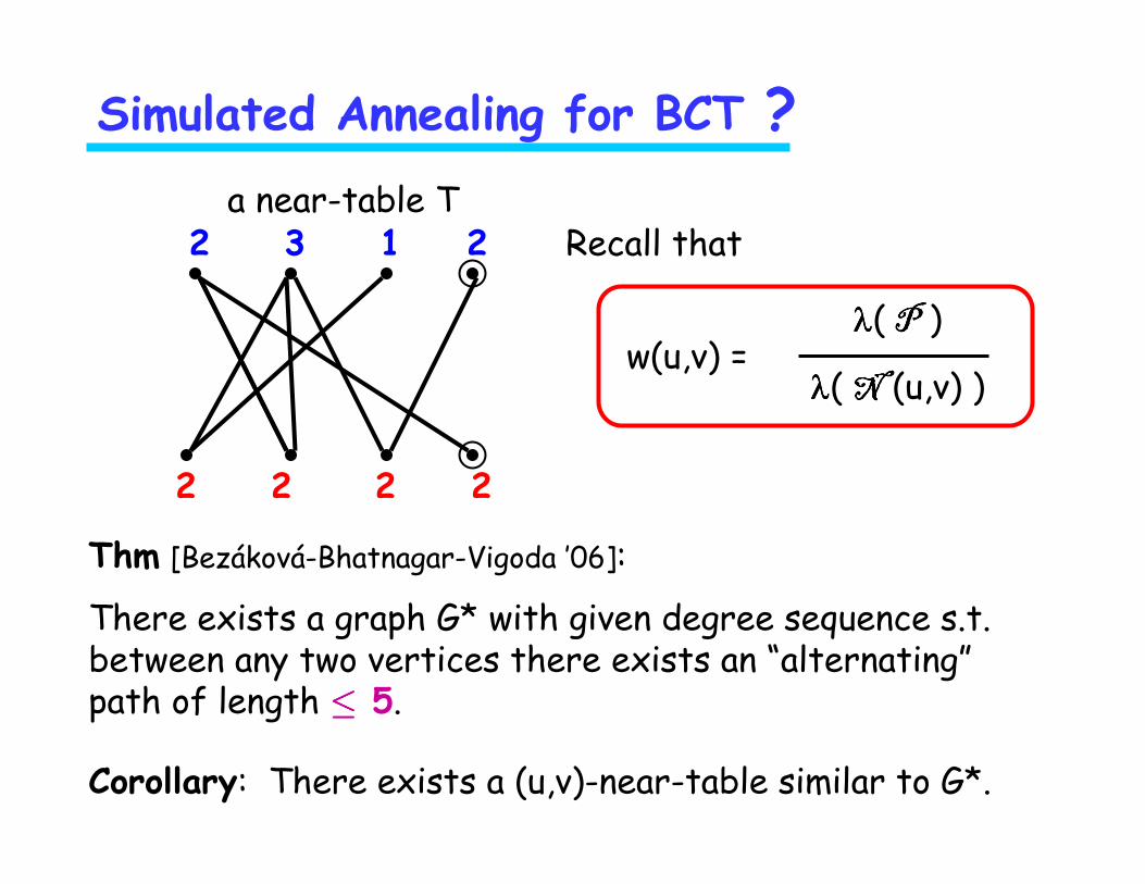
Corollary: There exists a (u,v)-near-table similar to G*.
Simulated Annealing for BCT ?
22 3 1
2 2 2 2
w(u,v) = λλλλ( P P P P )
λλλλ( N N N N (u,v) )
Recall that
Thm [Bezáková-Bhatnagar-Vigoda ’06]:
There exists a graph G* with given degree sequence s.t. between any two vertices there exists an “alternating”path of length ≤≤≤≤ 5.
a near-table T

Simulated Annealing for BCT ?
22 3 1
2 2 2 2
λλλλ w(u,v) = λλλλ( P P P P )
λλλλ( N N N N (u,v) )
Recall that
Thm [Bezáková-Bhatnagar-Vigoda ’06]:
There exists a graph G* with given degree sequence s.t. between any two vertices there exists an “alternating”path of length ≤≤≤≤ 5.
Corollary: λλλλ( N N N N (u,v) ) “easy” to compute for λλλλ = ~0.
G*
Simulated Annealing for BCT ?
22 3 1
2 2 2 2
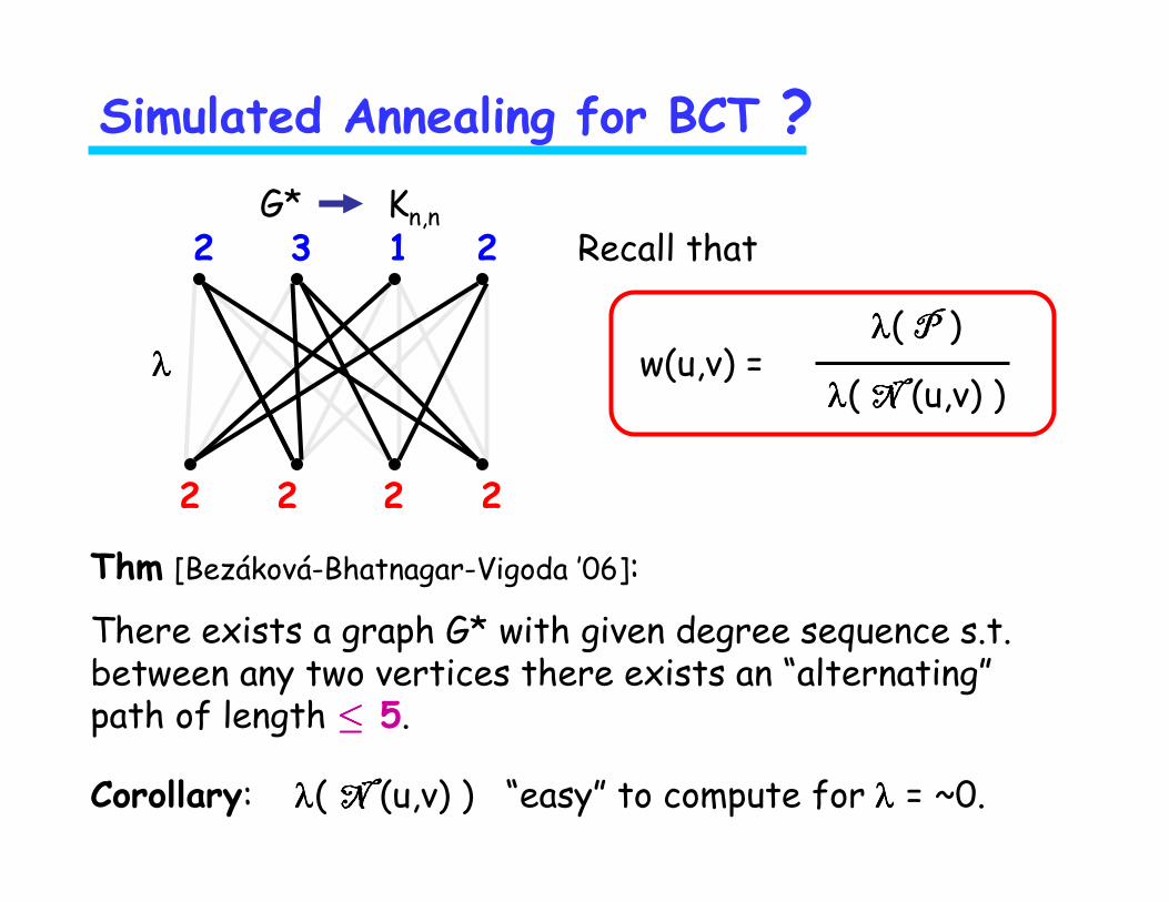
λλλλ w(u,v) = λλλλ( P P P P )
λλλλ( N N N N (u,v) )
Recall that
Thm [Bezáková-Bhatnagar-Vigoda ’06]:
There exists a graph G* with given degree sequence s.t. between any two vertices there exists an “alternating”path of length ≤≤≤≤ 5.
Corollary: λλλλ( N N N N (u,v) ) “easy” to compute for λλλλ = ~0.
G* Kn,n

Simulated Annealing for BCT ?
22 3 1
2 2 2 2
λλλλ w(u,v) = λλλλ( P P P P )
λλλλ( N N N N (u,v) )
Recall that
Thm [Bezáková-Bhatnagar-Vigoda ’06]:
There exists a graph G* with given degree sequence s.t. between any two vertices there exists an “alternating”path of length ≤≤≤≤ 5.
Corollary: λλλλ( N N N N (u,v) ) “easy” to compute for λλλλ = ~0.
G* Kn,n

Simulated Annealing for BCT ?
w(u,v) = λλλλ( P P P P )
λλλλ( N N N N (u,v) )
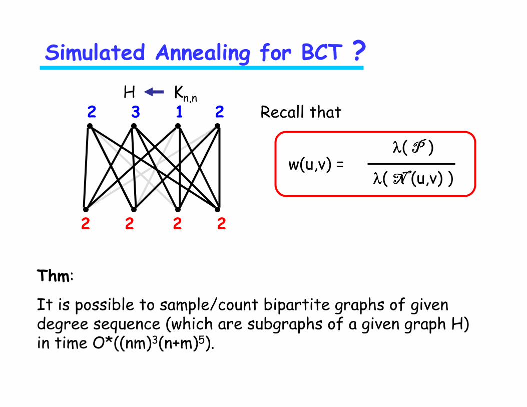
Recall thatH Kn,n
22 3 1
2 2 2 2
Thm:
It is possible to sample/count bipartite graphs of given degree sequence (which are subgraphs of a given graph H) in time O*((nm)3(n+m)5).

Simulated Annealing for BCT ?
w(u,v) = λλλλ( P P P P )
λλλλ( N N N N (u,v) )
Recall thatH Kn,n
22 3 1
2 2 2 2
Thm:
It is possible to sample/count bipartite graphs of given degree sequence (which are subgraphs of a given graph H) in time O*((nm)3(n+m)5).

Simulated Annealing for BCT ?
w(u,v) = λλλλ( P P P P )
λλλλ( N N N N (u,v) )
Recall thatH Kn,n
22 3 1
2 2 2 2
Thm:
It is possible to sample/count bipartite graphs of given degree sequence (which are subgraphs of a given graph H) in time O*((nm)3(n+m)5).

Simulated Annealing for BCT ?
w(u,v) = λλλλ( P P P P )
λλλλ( N N N N (u,v) )
Recall thatH Kn,n
22 3 1
2 2 2 2
Thm:
It is possible to sample/count bipartite graphs of given degree sequence (which are subgraphs of a given graph H) in time O*((nm)3(n+m)5).

Simulated Annealing for BCT ?
w(u,v) = λλλλ( P P P P )
λλλλ( N N N N (u,v) )
Recall thatH Kn,n
22 3 1
2 2 2 2
Thm:
It is possible to sample/count bipartite graphs of given degree sequence (which are subgraphs of a given graph H) in time O*((nm)3(n+m)5).

Simulated Annealing for BCT ?
w(u,v) = λλλλ( P P P P )
λλλλ( N N N N (u,v) )
Recall thatH Kn,n
22 3 1
2 2 2 2
Thm:
It is possible to sample/count bipartite graphs of given degree sequence (which are subgraphs of a given graph H) in time O*((nm)3(n+m)5).

Simulated Annealing for BCT ?
w(u,v) = λλλλ( P P P P )
λλλλ( N N N N (u,v) )
Recall thatH Kn,n
22 3 1
2 2 2 2
Thm:
It is possible to sample/count bipartite graphs of given degree sequence (which are subgraphs of a given graph H) in time O*((nm)3(n+m)5).
Simulated Annealing for BCT ?
w(u,v) = λλλλ( P P P P )
λλλλ( N N N N (u,v) )
Recall thatH Kn,n
22 3 1
2 2 2 2
Thm:
It is possible to sample/count bipartite graphs of given degree sequence (which are subgraphs of a given graph H) in time O*((nm)3(n+m)5).

Simulated Annealing for BCT ?
w(u,v) = λλλλ( P P P P )
λλλλ( N N N N (u,v) )
Recall thatH Kn,n
22 3 1
2 2 2 2
Thm:
It is possible to sample/count bipartite graphs of given degree sequence (which are subgraphs of a given graph H) in time O*((nm)3(n+m)5).

Different Approaches
Theory (Markov chain Monte Carlo with simulated annealing)
• Jerrum-Sinclair-Vigoda ’01: approximate permanent in O*(n10), yields O*((mn)10) algorithm for m x n binary contingency tables
• Bezáková-Bhatnagar-Vigoda ’06: O*((mn)3(m+n)5)
Practice (sequential importance sampling, Chen-Diaconis-Holmes-Liu ’05)
• Bezáková-Sinclair-Štefankovič-Vigoda ’06: negative example
• Jose Blanchet ’06: SIS works if marginals O(n1/4)
• Bayati-Kim-Saberi ’07: alternative importance sampling method, works if marginals O(n1/4)
Practice (the switching Markov chain, Diaconis-Gangolli ’94)
• Kannan-Tetali-Vempala ’97, Cooper-Dyer-Greenhill ’05: works for regular marginals
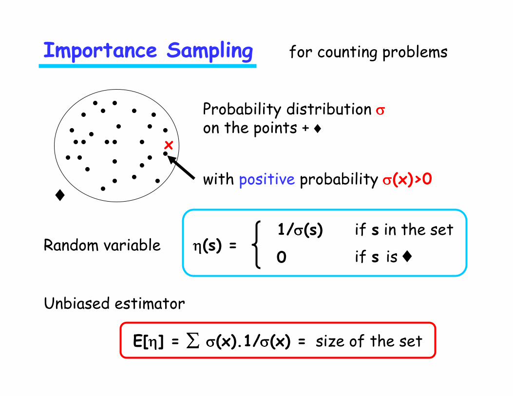
Importance Sampling for counting problems
x
with positive probability σσσσ(x)>0
Probability distribution σσσσon the points + ♦
♦
Random variable ηηηη(s) =1/σσσσ(s)
0
if s in the set
if s is ♦
Unbiased estimator
E[ηηηη] = ∑∑∑∑ σσσσ(x).1/σσσσ(x) = size of the set

2
3
21
3
32
5
3 4 2
4
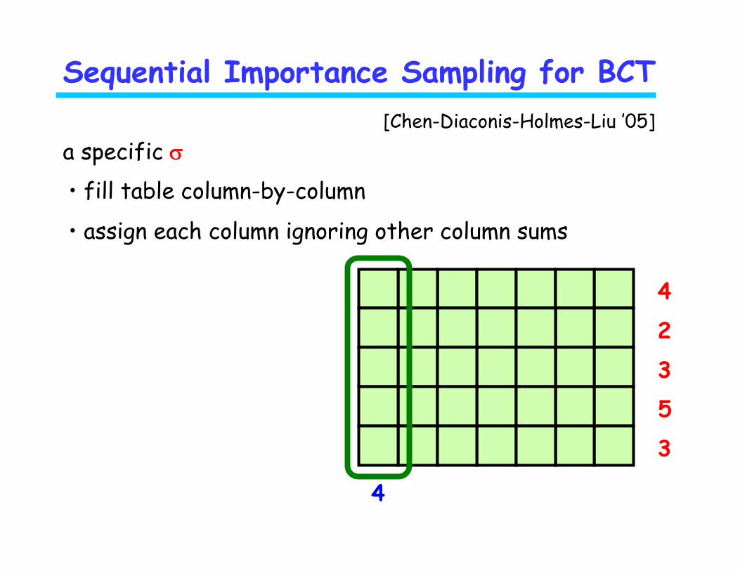
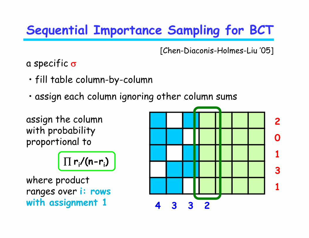
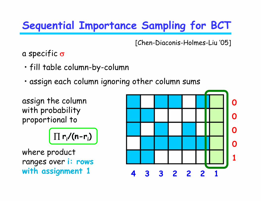
a specific σσσσ
• fill table column-by-column
• assign each column ignoring other column sums
[Chen-Diaconis-Holmes-Liu ’05]
Sequential Importance Sampling for BCT

2
3
22
3
12
5
4 3 3
4
a specific σσσσ
• fill table column-by-column
• assign each column ignoring other column sums
Sequential Importance Sampling for BCT
[Chen-Diaconis-Holmes-Liu ’05]

2
3
22
3
12
5
4 3 3
4
a specific σσσσ
• fill table column-by-column
• assign each column ignoring other column sums
Sequential Importance Sampling for BCT
[Chen-Diaconis-Holmes-Liu ’05]
2
3
3
5
4
4
a specific σσσσ
• fill table column-by-column
• assign each column ignoring other column sums
Sequential Importance Sampling for BCT
[Chen-Diaconis-Holmes-Liu ’05]
2
3
3
5
4
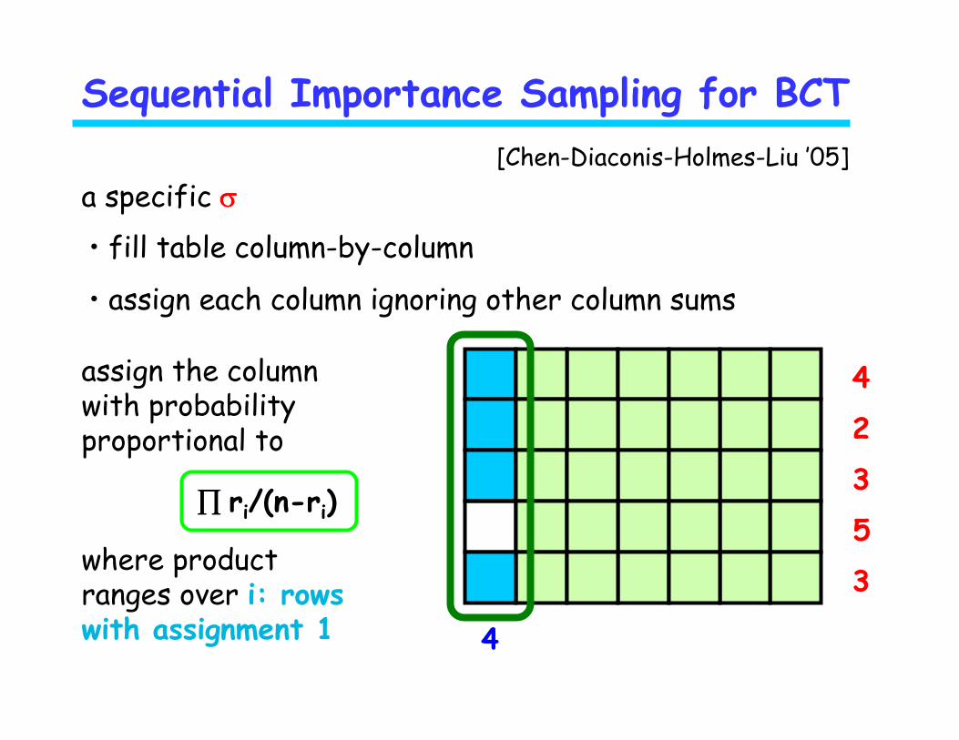
4assign the column with probability proportional to
a specific σσσσ
• fill table column-by-column
• assign each column ignoring other column sums
∏∏∏∏ ri/(n-ri)
where product ranges over i: rows with assignment 1
Sequential Importance Sampling for BCT
[Chen-Diaconis-Holmes-Liu ’05]
1
2
2
5
4
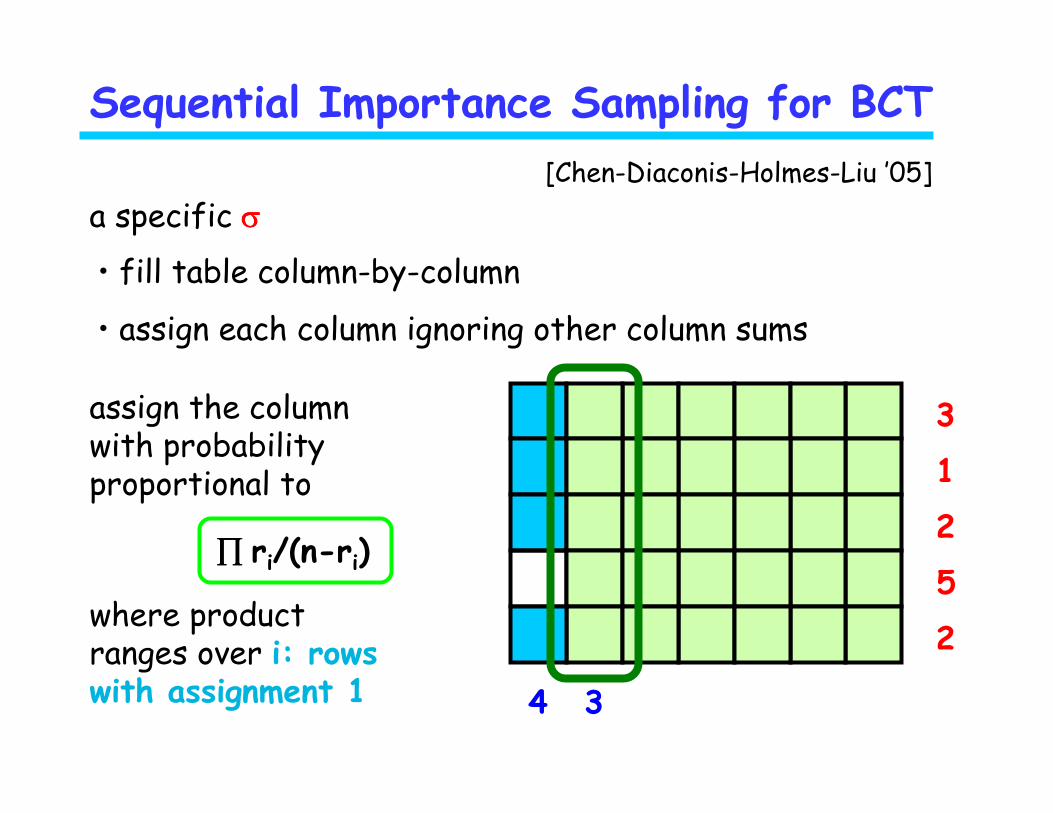
3assign the column with probability proportional to
a specific σσσσ
• fill table column-by-column
• assign each column ignoring other column sums
where product ranges over i: rows with assignment 1 3
∏∏∏∏ ri/(n-ri)
Sequential Importance Sampling for BCT
[Chen-Diaconis-Holmes-Liu ’05]
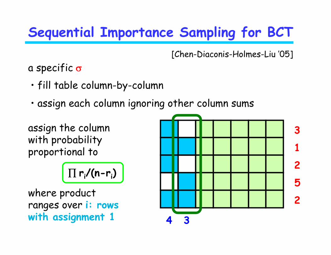
1
2
2
5
4
3assign the column with probability proportional to
a specific σσσσ
• fill table column-by-column
• assign each column ignoring other column sums
where product ranges over i: rows with assignment 1 3
∏∏∏∏ ri/(n-ri)
Sequential Importance Sampling for BCT
[Chen-Diaconis-Holmes-Liu ’05]

0
1
2
4
4
3assign the column with probability proportional to
a specific σσσσ
• fill table column-by-column
• assign each column ignoring other column sums
where product ranges over i: rows with assignment 1 3 3
∏∏∏∏ ri/(n-ri)
Sequential Importance Sampling for BCT
[Chen-Diaconis-Holmes-Liu ’05]

4
assign the column with probability proportional to
a specific σσσσ
• fill table column-by-column
• assign each column ignoring other column sums
where product ranges over i: rows with assignment 1 3 3
∏∏∏∏ ri/(n-ri)
0
1
2
4
3
Sequential Importance Sampling for BCT
[Chen-Diaconis-Holmes-Liu ’05]
0
1
1
3
4
2assign the column with probability proportional to
a specific σσσσ
• fill table column-by-column
• assign each column ignoring other column sums
where product ranges over i: rows with assignment 1 3 3 2
∏∏∏∏ ri/(n-ri)
Sequential Importance Sampling for BCT
[Chen-Diaconis-Holmes-Liu ’05]

4
assign the column with probability proportional to
a specific σσσσ
• fill table column-by-column
• assign each column ignoring other column sums
where product ranges over i: rows with assignment 1 3 3 2
∏∏∏∏ ri/(n-ri)
0
1
1
3
2
Sequential Importance Sampling for BCT
[Chen-Diaconis-Holmes-Liu ’05]

0
1
1
2
4
1assign the column with probability proportional to
a specific σσσσ
• fill table column-by-column
• assign each column ignoring other column sums
where product ranges over i: rows with assignment 1 3 3 22
∏∏∏∏ ri/(n-ri)
Sequential Importance Sampling for BCT
[Chen-Diaconis-Holmes-Liu ’05]

4
assign the column with probability proportional to
a specific σσσσ
• fill table column-by-column
• assign each column ignoring other column sums
where product ranges over i: rows with assignment 1 3 3 22
∏∏∏∏ ri/(n-ri)
0
1
1
2
1
Sequential Importance Sampling for BCT
[Chen-Diaconis-Holmes-Liu ’05]

0
1
0
1
4
1assign the column with probability proportional to
a specific σσσσ
• fill table column-by-column
• assign each column ignoring other column sums
where product ranges over i: rows with assignment 1 3 3 22 2
∏∏∏∏ ri/(n-ri)
Sequential Importance Sampling for BCT
[Chen-Diaconis-Holmes-Liu ’05]

4
assign the column with probability proportional to
a specific σσσσ
• fill table column-by-column
• assign each column ignoring other column sums
where product ranges over i: rows with assignment 1 3 3 22 2
∏∏∏∏ ri/(n-ri)
0
1
0
1
1
Sequential Importance Sampling for BCT
[Chen-Diaconis-Holmes-Liu ’05]
0
1
0
0
4
0assign the column with probability proportional to
a specific σσσσ
• fill table column-by-column
• assign each column ignoring other column sums
where product ranges over i: rows with assignment 1 3 3 22 2 1
∏∏∏∏ ri/(n-ri)
Sequential Importance Sampling for BCT
[Chen-Diaconis-Holmes-Liu ’05]

4
assign the column with probability proportional to
a specific σσσσ
• fill table column-by-column
• assign each column ignoring other column sums
where product ranges over i: rows with assignment 1 3 3 22 2 1
∏∏∏∏ ri/(n-ri)
0
1
0
0
0
Sequential Importance Sampling for BCT
[Chen-Diaconis-Holmes-Liu ’05]

Sequential Importance Sampling for BCT
4
assign the column with probability proportional to
a specific σσσσ
• fill table column-by-column
• assign each column ignoring other column sums
where product ranges over i: rows with assignment 1 3 3 22 2 1
∏∏∏∏ ri/(n-ri)
0
0
0
0
0
[Chen-Diaconis-Holmes-Liu ’05]

Sequential Importance Sampling for BCT
4
assign the column with probability proportional to
a specific σσσσ
• fill table column-by-column
• assign each column ignoring other column sums
where product ranges over i: rows with assignment 1 3 3 22 2 1
∏∏∏∏ ri/(n-ri)
2
3
3
5
4
[Chen-Diaconis-Holmes-Liu ’05]

A Counterexample for SIS
1 1 1 11 1 γγγγm
1
ββββm
1
1
1
Thm [Bezáková-Sinclair-Štefankovič-Vigoda ‘06]:
For any ββββ ≠≠≠≠ γγγγ, SIS output after any subexponentialnumber of trials is off by an exponential factor(with high probability).

A Counterexample for SIS
1 1 1 11 1
1
ββββm
1
1
1
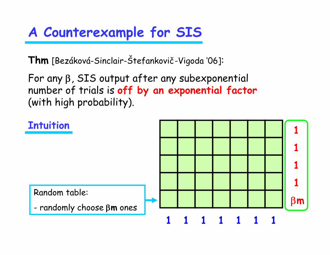
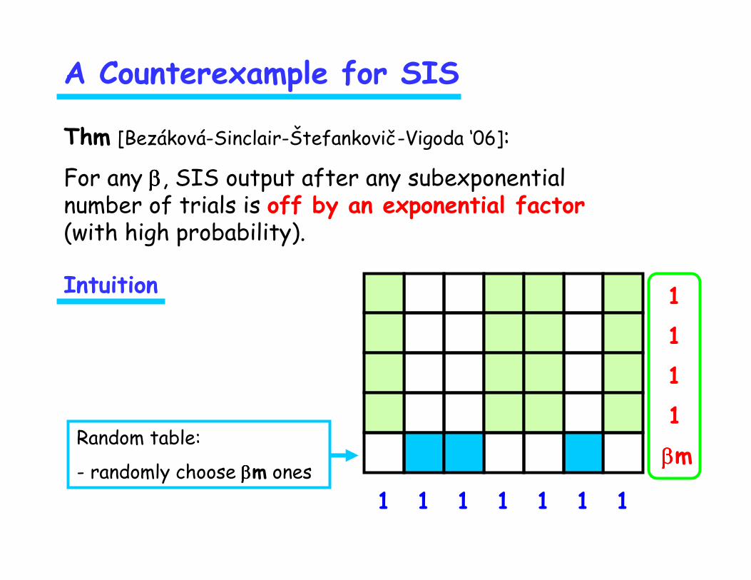
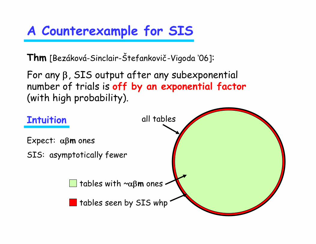
Thm [Bezáková-Sinclair-Štefankovič-Vigoda ‘06]:
For any ββββ, SIS output after any subexponentialnumber of trials is off by an exponential factor(with high probability).
Simpler example
1
A Counterexample for SIS
1 1 1 11 1
1
ββββm
1
1
1Intuition
1
Random table:
- randomly choose ββββm ones
Thm [Bezáková-Sinclair-Štefankovič-Vigoda ‘06]:
For any ββββ, SIS output after any subexponentialnumber of trials is off by an exponential factor(with high probability).

A Counterexample for SIS
1 1 1 11 1
1
ββββm
1
1
1Intuition
1
Random table:
- randomly choose ββββm ones
Thm [Bezáková-Sinclair-Štefankovič-Vigoda ‘06]:
For any ββββ, SIS output after any subexponentialnumber of trials is off by an exponential factor(with high probability).
A Counterexample for SIS
1 1 1 11 1
1
ββββm
1
1
1Intuition
1
Random table:
- randomly choose ββββm ones
Thm [Bezáková-Sinclair-Štefankovič-Vigoda ‘06]:
For any ββββ, SIS output after any subexponentialnumber of trials is off by an exponential factor(with high probability).

A Counterexample for SIS
1 1 1 11 1
1
ββββm
1
1
1Intuition
1
Random table:
- randomly choose ββββm ones
ααααm
Expect: αβαβαβαβm ones
SIS: asymptotically fewer
Thm [Bezáková-Sinclair-Štefankovič-Vigoda ‘06]:
For any ββββ, SIS output after any subexponentialnumber of trials is off by an exponential factor(with high probability).
A Counterexample for SIS
Intuition
Expect: αβαβαβαβm ones
SIS: asymptotically fewer
all tables
tables with ~αβαβαβαβm ones
tables seen by SIS whp
Thm [Bezáková-Sinclair-Štefankovič-Vigoda ‘06]:
For any ββββ, SIS output after any subexponentialnumber of trials is off by an exponential factor(with high probability).

A Counterexample for SIS
1 1 1 11 1 γγγγm
1
ββββm
1
1
1
Thm [Bezáková-Sinclair-Štefankovič-Vigoda ‘06]:
For any ββββ ≠≠≠≠ γγγγ, SIS output after any subexponentialnumber of trials is off by an exponential factor(with high probability).
Result holds for any order of rows/columns.
Alternating rows and columns?

50 100 150 200 250 300 350
201
202
203
204
205
206
SIS – Experimental Results
Bad example, m = 300, ββββ = 0.6, γγγγ = 0.7
log-scaleof SIS estimate
number SIS steps
correct

• Practical algorithm ?
• Detecting convergence of SIS
• SIS for larger marginals ?
• The Switching Markov chain of Diaconis-Gangolli ?
• General contingency tables
• Cell-bounded tables
• Counting non-bipartite graphs with a given degree sequence
Open Problems


![Winter Contingency Plan 2019 - PDMA Contingency... · 2020. 12. 24. · [KHYBER PAKHTUNKHWA WINTER CONTINGENCY PLAN 2019-20] Winter Contingency Plan 5 | Page utilizing PAF strategic](https://static.cupdf.com/doc/110x72/611400065caf3c03a80f7591/winter-contingency-plan-2019-pdma-contingency-2020-12-24-khyber-pakhtunkhwa.jpg)