Big Data Technology
Big Data
"Big data" is a field that treats ways to analyze, systematically extract information 1
from, or otherwise deal with data sets that are too large or complex to be dealt with by
traditional data-processing application software. Data with many cases (rows) offer
greater statistical power, while data with higher complexity (more attributes or columns,
i.e., structured, semi-structured or unstructured) may lead to a higher false discovery
rate. Big data challenges include capturing data, data storage, data analysis, search,
sharing, transfer, visualization, querying, updating, information privacy and data
source. Big data was originally associated with three key concepts: 3V:- volume, variety, and velocity. Other concepts later attributed with big data are veracity (i.e., how much
noise is in the data) and value.
Current usage of the term big data tends to refer to the use of predictive analytics, user
behavior analytics, or certain other advanced data analytics methods that extract value
from data. Analysis of data sets can find new correlations to "spot business trends,
prevent diseases, combat crime and so on.
Big data usually includes data sets with sizes beyond the ability of commonly used
software tools to capture, manage, and process data within a tolerable elapsed time.Big
data philosophy encompasses unstructured, semi-structured and structured data,
however the main focus is on unstructured data. Big data "size" is a constantly moving
target, big data requires a set of techniques and technologies with new forms of
integration to reveal insights from datasets that are diverse, complex, and of a massive
scale.
Technologies
The big data analytics technology is a combination of several techniques and processing
methods. The technologies in big data can include types of software, tools for some form
of data analysis, hardware for better data processing, products, methods and myriad of
other technologies. Big data is basically a term to represent a huge volume of data, and
data is always growing, so are its applicable technologies like distributed file systems
(GFS, HDFS) and also distributed computing models (MAP/REDUCE, NO SQL, etc).
1
[email protected] | All Rights Reserved 0
Table of Content
1. Introduction to Big Data
1.1. Big Data Overview
1.2. Background of Data Analytics
1.3. Role of Distributed System in Big Data
1.4. Role of Data Scientist
1.5. Current trend in Big Data Analytics
2. Google File System
2.1. Introduction to Distributed File System
2.2. GFS cluster and Commodity Hardware
2.3. GFS Architecture
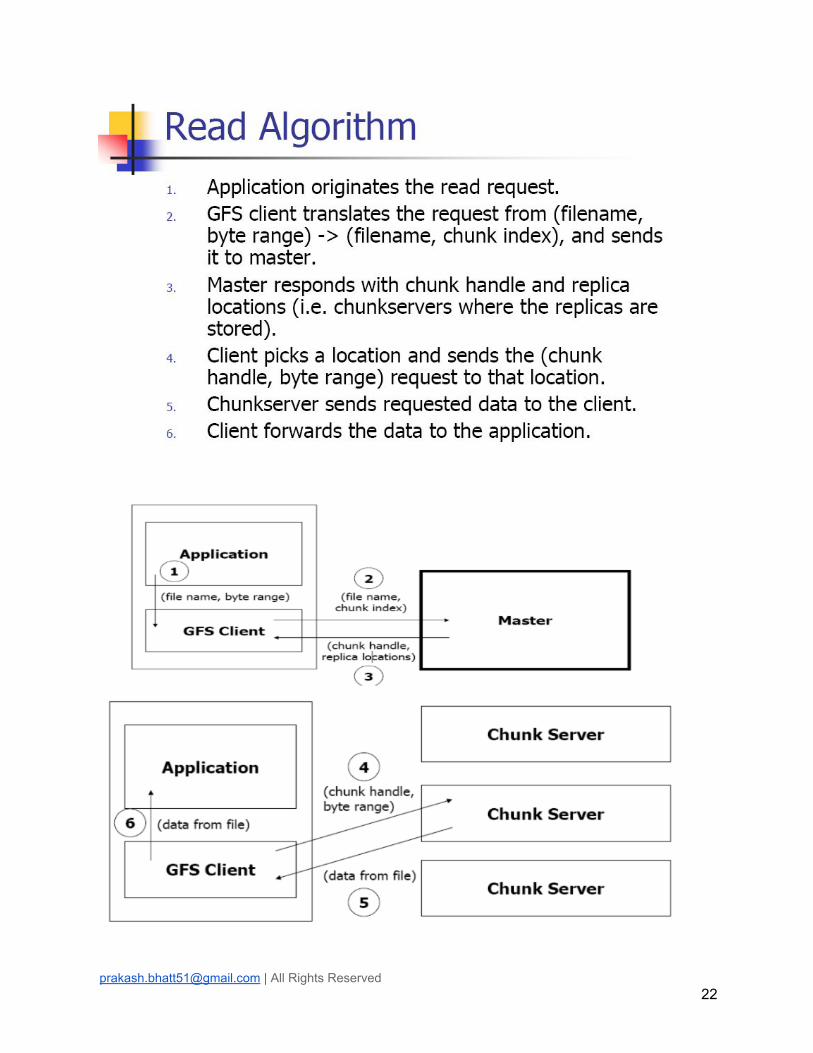
2.4. Data Read Algorithm
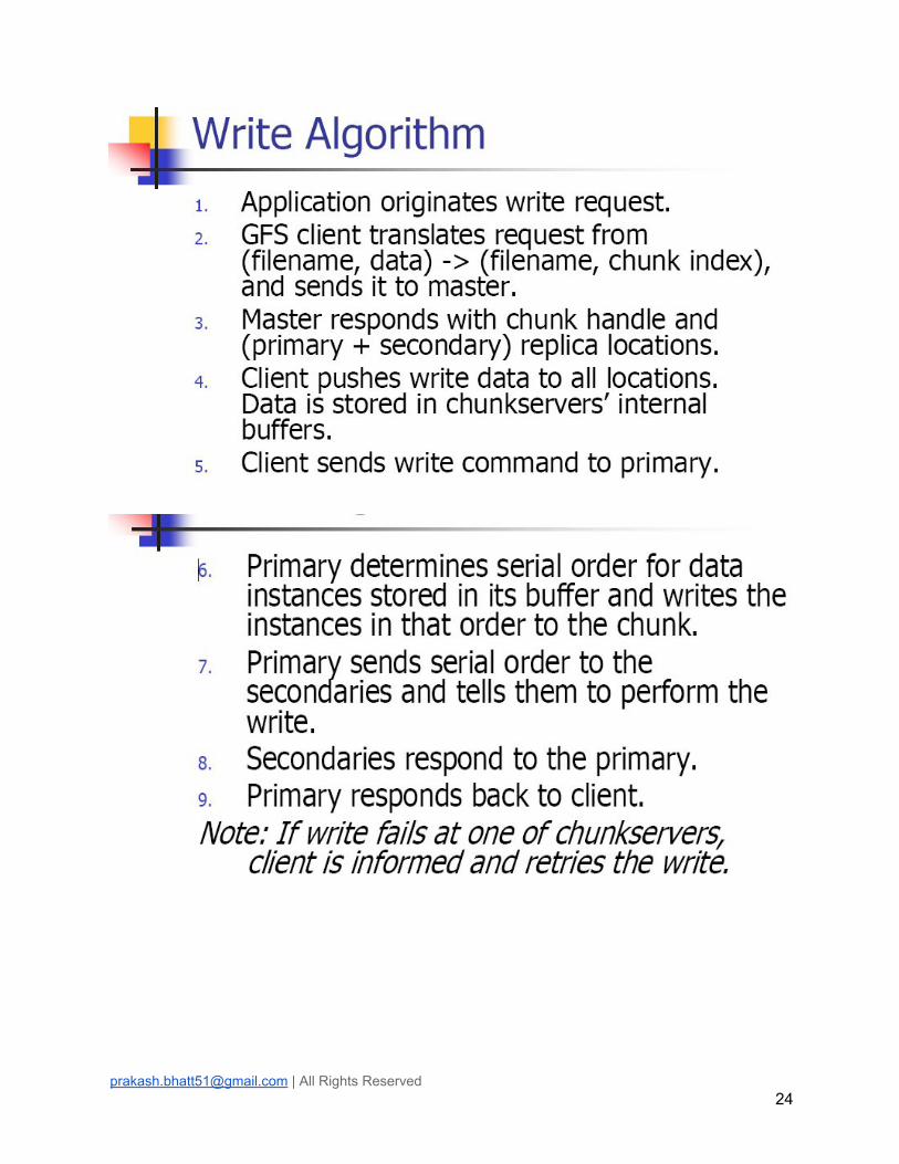
2.5. Data Write Algorithm
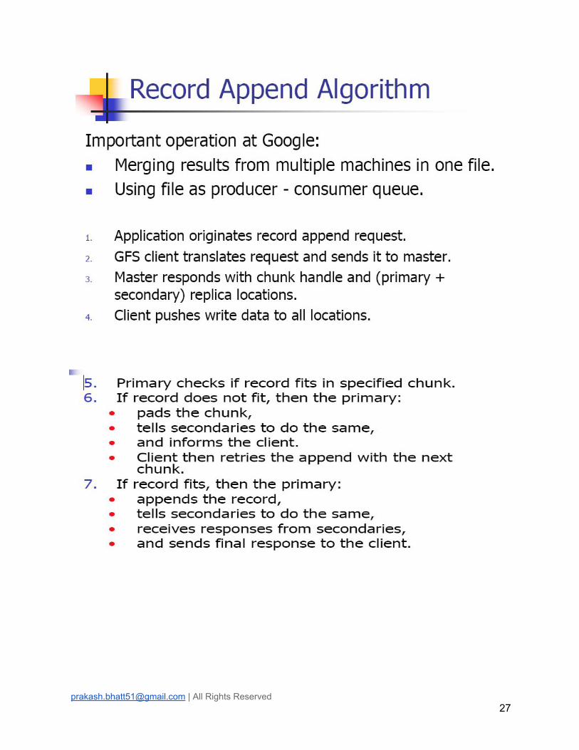
2.6. Record Append Algorithm
2.7. Common Goals of GFS
2.8. Data Availability
2.9. Fault Tolerance File System
2.10. Optimization for Large Scale Data
2.11. Data Consistency Model
2.12. Data Integrity
2.13. Data Replication, Re-replication and Rebalance
2.14. Garbage Collection
2.15. Real World Clusters
3. Map Reduce Framework
3.1. Basics of functional Programming
3.2. First class functions and Higher order Functions
3.3. Real World Problem Solving Techniques in FP
3.4. Build in Function map() and reduce()
3.5. Map Reduce Data Flow and Working Architecture
3.6. Steps in Map Reduce
3.7. Library Functions and classes in Map Reduce
3.8. Problem Solving Techniques
3.9. Parallel Efficiency in Map Reduce
3.10. Examples
[email protected] | All Rights Reserved 1

4. Hadoop
4.1. Introduction to Hadoop Environment
4.2. Hadoop Distributed File System
4.3. Common Goals of Hadoop
4.4. Hadoop Daemons
4.5. Hadoop Installation Process
4.6. Hadoop Configuration Modes
4.7. Hadoop Shell Commands
4.8. Hadoop IO and Data Flow
4.9. Query Languages for Hadoop
4.10. Hadoop and Map Reduce
4.11. Hadoop and Amazon Cloud
5. NO SQL Technology
5.1. Introduction to NO SQL Technology
5.2. Data Distribution and Replication in NO SQL
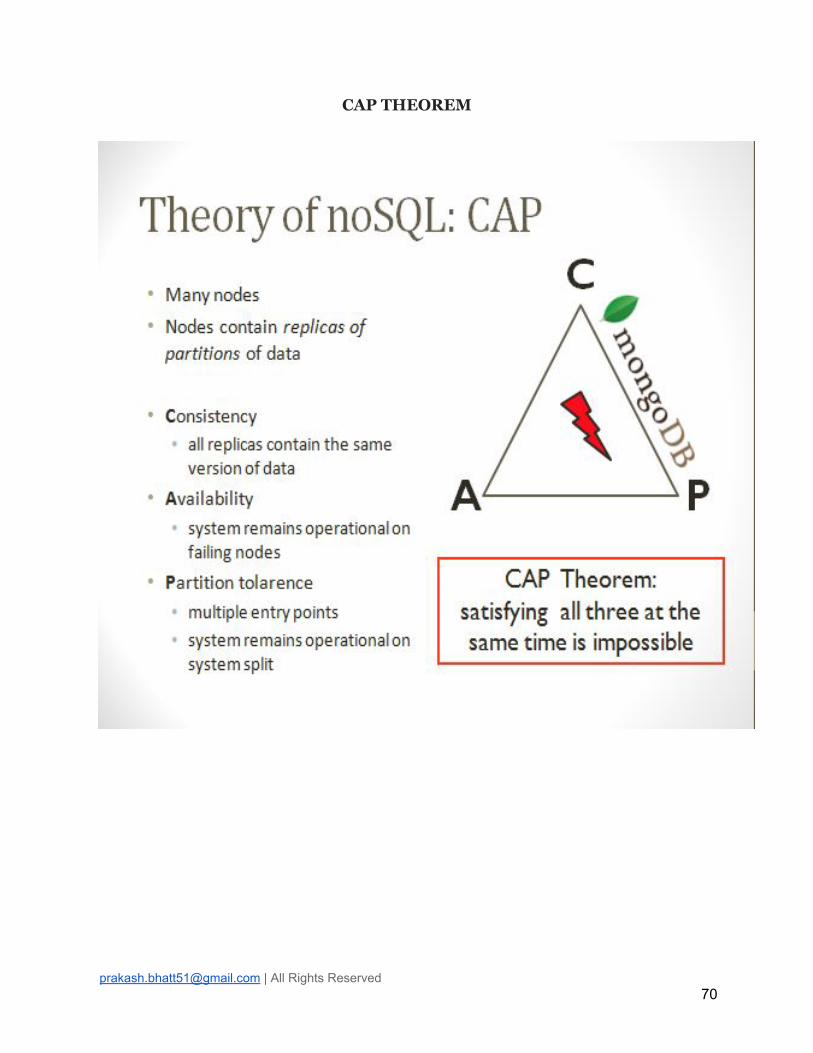
5.3. CAP Theorem
5.4. HBASE
5.5. Cassandra
5.6. MongoDB
6. Searching and Indexing
6.1. Data Searching
6.2. Data Indexing
6.3. Lucene
6.4. Data Indexing with Lucene
6.5. Distributed Searching
6.6. Data Searching with ElasticSearch
[email protected] | All Rights Reserved 2

1. Introduction to Big Data
1.1. Big Data Overview
Big data is a term applied to a new generation of software applications, and
storage architecture. It is designed to provide business value from structured, semi structured and unstructured data. Big data sets require advanced tools, software,
and systems to capture, store, manage, and analyze the data sets, All in a timeframe Big
data preserves the intrinsic value of the data. Big data is now applied more
broadly to cover commercial environments.
Four distinct applications segments comprise the big data market. Each with varying
levels of need for performance and scalability.
[email protected] | All Rights Reserved 3

The four big data segments are:
1. Design (engineering collaboration)
2. Discover (core simulation – supplanting physical experimentation)
3. Decide (analytics).
4. Deposit (Web 2.0 and data warehousing)
Figure: Big Data Application Segments
[email protected] | All Rights Reserved 4

1.2 Background of Data Analytics
Big data analytics is the process of examining large amounts of data of a variety of types.
The primary goal of big data analytics is to help companies make better business
decisions. Analyze huge volumes of transaction data as well as other data sources that
may be left untapped by conventional business intelligence (BI) programs.
Big Data consist of following
1. Uncovered hidden patterns.
2. Unknown correlations and other useful information. Such information can
provide business benefits.
3. More effective marketing and increased revenue.
Big data analytics can be done with the software tools commonly used as part of
advanced analytics disciplines, such as predictive analysis and data mining. But the
unstructured data sources used for big data analytics may not fit in traditional data
warehouses. Traditional data warehouses may not be able to handle the processing
demands posed by big data.
Technologies associated with big data analytics include NO SQL databases, Hadoop and
MapReduce, etc. Known about these technologies form the core of an open source
software framework that supports the processing of large data sets across clustered
systems. Big data analytics initiatives include internal data analytics skills high cost of
hiring experienced analytics professionals, challenges in integrating Hadoop systems
and data warehouses.
Big Analytics delivers competitive advantage in two ways compared to the traditional
analytical model.
1. Big Analytics describes the efficient use of a simple model applied to volumes of
data that would be too large for the traditional analytical environment.
2. Research suggests that a simple algorithm with a large volume of data is more
accurate than a sophisticated algorithm with little data.
Data Analytics supporting the following objectives for working with large volumes of
data.
1. Avoid sampling and aggregation;
2. Reduce data movement and replication
3. Bring the analytics as close as possible to the data
4. Optimize computation speed
[email protected] | All Rights Reserved 8

The Power and Promise of Analytics
Business Intelligence uses big data and analytics for these purposes
1. Big Data Analytics to Improve Network Security.
2. Security professionals manage enterprise system risks by
controlling access to systems, services and applications defending
against external threats.
3. Protecting valuable data and assets from theft and loss.
4. Monitoring the network to quickly detect and recover from an
attack.
5. Big data analytics is particularly important to network monitoring,
auditing and recovery.
Examples; 1. Reducing Patient Readmission Rates (Medical data)
Big data to address patient care issues and to reduce hospital readmission rates.
The focus on lack of follow-up with patients, medication management issues and
insufficient coordination of care. Data is preprocessed to correct any errors and to
format it for analysis.
2. Analytics to Reduce the Student Dropout Rate (Educational Data)
Analytics applied to education data can help schools and school systems better
understand how students learn and succeed. Based on these insights, schools and school
systems can take steps to enhance education environments and improve outcomes.
Assisted by analytics, educators can use data to assess and when necessary re-organize
classes, identify students who need additional feedback or attention. Direct resources to
students who can benefit most from them.
[email protected] | All Rights Reserved 9

Data Analytics Process
Knowledge discovery phase involves (PHASE 1):
1. Gathering data to be analyzed.
2. Pre-processing it into a format that can be used.
3. Consolidating (more certain) it for analysis, analyzing it to discover what it may
reveal.
4. Interpreting it to understand the processes by which the data was analyzed and
how conclusions were reached.
Acquisition –(process of getting something)
Data acquisition involves collecting or acquiring data for analysis. Acquisition requires
access to information and a mechanism for gathering it.
Pre-processing
Data is structured and entered into a consistent format that can be analyzed.
Pre-processing is necessary if analytics is to yield trustworthy (able to trusted), useful
results. Data are stored in a standard format for further analysis.
[email protected] | All Rights Reserved 10

Integration
Integration involves:
1. Consolidating data for analysis.
2. Retrieving relevant data from various sources for analysis
3. Eliminating redundant data or clustering data to obtain a smaller representative
sample.
4. Clean data into its data warehouse and further organizes it to make it readily
useful for research.
5. Distillation into manageable samples.
Analysis
Knowledge discovery involves:
1. Searching for relationships between data items in a database, or exploring data in
search of classifications or associations.
2. Analysis can yield descriptions (where data is mined to characterize properties)
or predictions (where a model or set of models is identified that would yield
predictions).
3. Analysis based on interpretation, organizations can determine whether and how
to act on them.
Interpretation
1. Analytic processes are reviewed by data scientists to understand results and how
they were determined.
2. Interpretation involves retracing methods, understanding choices made
throughout the process and critically examining the quality of the analysis.
3. It provides the foundation for decisions about whether analytic outcomes are
trustworthy
The product of the knowledge discovery phase is an algorithm. Algorithms can perform
a variety of tasks:
1. Classification algorithms: Categorize discrete variables (such as classifying
an incoming email as spam).
[email protected] | All Rights Reserved 11

2. Regression algorithms: Calculate continuous variables (such as the value of a
home based on its attributes and location).
3. Segmentation algorithms: Divide data into groups or clusters of items that
have similar properties (such as tumors found in medical images).
4. Association algorithms: Find correlations between different attributes in a
data set (such as the automatically suggested search terms in response to a
query).
5. Sequence analysis algorithms : Summarize frequent sequences in data (such
as understanding a DNA sequence to assign function to genes and proteins by
comparing it to other sequences).
Application (PHASE 2)
In the application phase organizations reap (collect) the benefits of knowledge
discovery. Through application of derived algorithms, organizations make
determinations upon which they can act.
1.3 Data Scientist
Data scientist includes:
1. Data capture and Interpretation
2. New analytical techniques
3. Community of Science
4. Perfect for group work
5. Teaching strategies
6. Wide range of skills:
a. Business domain expertise and strong analytical skills
b. Creativity and good communications.
c. Knowledgeable in statistics, machine learning and data visualization
d. Able to develop data analysis solutions using modeling/analysis methods
and languages such as Map-Reduce, R, SAS, etc.
e. Adept at data engineering, including discovering and mashing/blending
large amounts of data.
f. Adept at data engineering, including discovering and mashing/blending
large amounts of data.
[email protected] | All Rights Reserved 12

Role of Data Scientist:
Data scientist helps broaden the business scope of investigative computing in three
areas:
1. New sources of data – supports access to multi-structured data.
2. New and improved analysis techniques – enables sophisticated analytical
processing of multi-structured data using techniques such as Map-Reduce and
in-database analytic functions.
3. Improved data management and performance – provides improved
price/performance for processing multi-structured data using non-relational
systems such as Hadoop, relational DBMSs, and integrated hardware/software.
[email protected] | All Rights Reserved 13

1.4 Role of Distributed System in Big Data
The amount of available data has exploded significantly in the past years, due to the fast
growing number of services and users producing vast amounts of data. The explosion of
devices that have automated and perhaps improved the lives of all of us has generated a
huge mass of information that will continue to grow exponentially.
For this reason, the need to store, manage, and treat the ever increasing amounts of data
has become urgent. The challenge is to find a way to transform raw data into valuable
information. To capture value from those kind of data, it is necessary to have an
innovation in technologies and techniques that will help individuals and organizations
to integrate, analyze, visualize different types of data at different spatial and temporal
scales.
Distributed Computing together with management and parallel processing principle
allow to acquire and analyze intelligence from Big Data making Big Data Analytics a
reality. Different aspects of the distributed computing paradigm resolve different types
of challenges involved in Analytics of Big Data.
Distributed Computing and storage required to meet the following constraints
1. Time constraint
2. Response time
3. Data Availability
4. Scalability
5. System performance
1.5 Current trend in Big Data Analytics
1. Iterative process (Discovery and Application)
2. Analyze the structured/semi-structured/unstructured data (Data analytics)
3. development of algorithm (Data analytics)
4. Data refinement (Data scientist)
5. Algorithm implementation using distributed engine. E.g. HDFS (S/W engineer)
and use NO SQL DB (Elasticsearch, Hbase, MangoDB, Cassandra, etc)
6. Visual presentation in Application Software
7. Application verification
[email protected] | All Rights Reserved 14

2. Google File System
Google File System, a scalable distributed file system for large distributed
data-intensive applications. GFS meets the rapidly growing demands of Google’s data
processing needs. It shares many of the same goals as other distributed file systems such
as performance, scalability, reliability, and availability. And provides a familiar file
system interface. Files are organized hierarchically in directories and identified by
pathnames. GFS supports the usual operations like create, delete, open, close, read, and
write files.
[email protected] | All Rights Reserved 15

Common Goals of GFS
Common goals of GFS are as follows
1. Performance
2. Reliability
3. Scalability
4. Availability
GFS Concepts:
1. Small as well as multi-GB files are common.
2. Each file typically contains many application objects such as web documents.
3. GFS provides an atomic append operation called record append. In a traditional
write, the client specifies the offset at which data is to be written.
4. Concurrent writes to the same region are not serializable.
5. GFS has snapshot and record append operations.
6. The snapshot operation makes a copy of a file or a directory.
7. Record append allows multiple clients to append data to the same file
concurrently while guaranteeing the atomicity of each individual client’s append.
8. It is useful for implementing multi-way merge results.
9. GFS consist of two kinds of reads: large streaming reads and small random reads.
10. In large streaming reads, individual operations typically read hundreds of KBs,
more commonly 1 MB or more.
11. A small random read typically reads a few KBs at some arbitrary offset.
12. Component failures are the norm rather than the exception. Why
assume hardware failure is the norm?
File System consists of hundreds or even thousands of storage machines built
from inexpensive commodity parts. It is cheaper to assume common failure on
poor hardware and account for it, rather than invest in expensive hardware
and still experience occasional failure.
The amount of layers in a distributed system (network, disk, memory, physical
connections, power, OS, application) mean failure on any could contribute to
data corruption.
13. Files are Huge. Multi-GB Files are common. Each file typically contains many application objects such as web documents.
14. Append, Append, Append. 15. Most files are mutated by appending new data rather than overwriting
existing data.
[email protected] | All Rights Reserved 17

16. Co-Designing
Co-designing applications and file system API benefits overall system by
increasing flexibility.
GFS Architecture
A GFS cluster consists of a single master and multiple chunk-servers and is accessed by
multiple clients, Each of these is typically a commodity Linux machine. It is easy to run
both a chunk-server and a client on the same machine. As long as machine resources
permit, it is possible to run flaky application code is acceptable. Files are divided into
fixed-size chunks.
Each chunk is identified by an immutable and globally unique 64 MB chunk assigned
by the master at the time of chunk creation. Chunk-servers store chunks on local disks
as Linux files, each chunk is replicated on multiple chunk-servers.
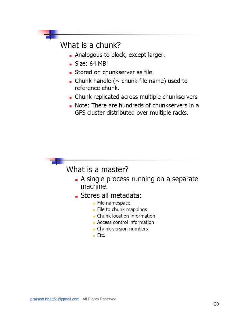
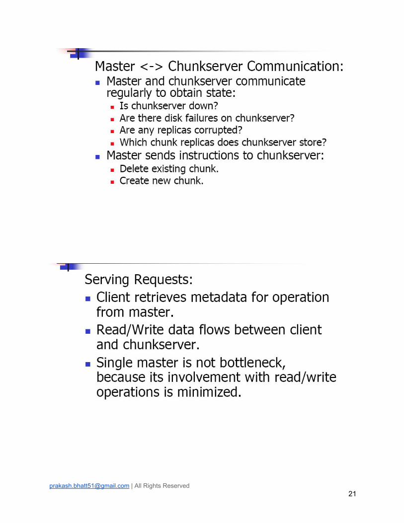
The master maintains all file system metadata. This includes the namespace, access
control information, mapping from files to chunks, and the current locations of
chunks. It also controls chunk migration between chunk servers.
The master periodically communicates with each chunk server in HeartBeat messages
to give it instructions and collect its state.
[email protected] | All Rights Reserved 18

3. Map Reduce Framework
Introduction Map-Reduce is a programming model designed for processing large volumes of data in
parallel by dividing the work into a set of independent tasks. Map-Reduce programs are
written in a particular style influenced by functional programming constructs,
specifically idioms for processing lists of data. This module explains the nature of this
programming model and how it can be used to write programs which run in the Hadoop
environment.
Functional Programming and List Processing
Conceptually, Map-Reduce programs transform lists of input data elements into lists of
output data elements. A Map-Reduce program will do this twice, using two different list
processing idioms: map, and reduce. These terms are taken from several list processing
languages such as LISP, Scheme, or ML.
As software becomes more and more complex, it is more and more important to
structure it well.
Well-structured software is easy to write and to debug, and provides a collection of
modules that can be reused to reduce future programming costs.
Map-Reduce has its roots in functional programming, which is exampled in languages
such as Lisp and ML. As software becomes more and more complex, it is more and
more important to structure it well. Well-structured software is easy to write and to
debug, and provides a collection of modules that can be reused to reduce future
programming costs. Map-Reduce has its roots in functional programming, which is
exampled in languages such as Lisp and ML.
Examples
// Regular Style
Integer timesTwo(Integer i) {
return i * 2;
}
[email protected] | All Rights Reserved 37
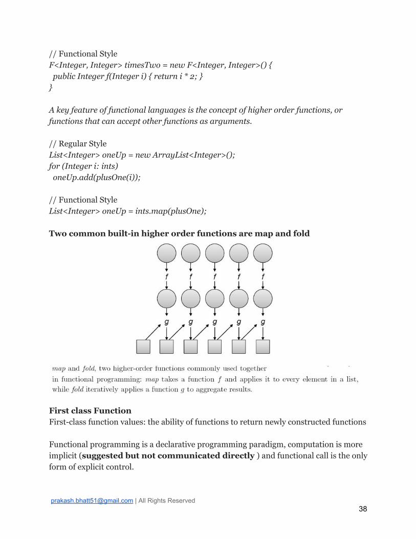
// Functional Style
F<Integer, Integer> timesTwo = new F<Integer, Integer>() {
public Integer f(Integer i) { return i * 2; }
}
A key feature of functional languages is the concept of higher order functions, or
functions that can accept other functions as arguments.
// Regular Style
List<Integer> oneUp = new ArrayList<Integer>();
for (Integer i: ints)
oneUp.add(plusOne(i));
// Functional Style
List<Integer> oneUp = ints.map(plusOne);
Two common built-in higher order functions are map and fold
First class Function
First-class function values: the ability of functions to return newly constructed functions
Functional programming is a declarative programming paradigm, computation is more
implicit (suggested but not communicated directly ) and functional call is the only
form of explicit control.
[email protected] | All Rights Reserved 38

Many (commercial) applications exist for functional programming:
1. Symbolic data manipulation
2. Natural language processing
3. Artificial intelligence
4. Automatic theorem proving and computer algebra
5. Algorithmic optimization of programs written in pure functional languages (e.g
Map-reduce)
6. Functional programming languages are Compiled and/or interpreted
7. Have simple syntax Use garbage collection for memory management
8. Are statically scoped or dynamically scoped
9. Use higher-order functions and subroutine closures
10. Use first-class function values
11. Depend heavily on polymorphism
Origin of Functional Programming
Church’s thesis:
All models of computation are equally powerful and can compute any function
Turing’s model of computation: Turing machine Reading/writing of values on an
infinite tape by a finite state machine
Church’s model of computation: lambda calculus
This inspired functional programming as a concrete implementation of lambda
calculus.
Computability theory:
A program can be viewed as a constructive proof that some mathematical object with a
desired property exists. A function is a mapping from input to output objects and
computes output objects from appropriate inputs.
Functional programming defines the outputs of a program as a mathematical function
of the inputs with no notion of internal state (no side effects ). A pure function can
always be counted on to return the same results for the same input parameters
No assignments: dangling and/or uninitialized pointer references do not occur
Example pure functional programming languages are : Miranda , Haskell , and
Sisal. Non-pure functional programming languages include imperative features with
side effects that affect global state (e.g. through destructive assignments to global
variables). Example: Lisp , Scheme , and ML.
[email protected] | All Rights Reserved 39

Useful features are found in functional languages that are often missing in imperative
languages:
1. First-class function values: the ability of functions to return newly
constructed functions
2. Higher-order functions : functions that take other functions as input
parameters or return functions.
3. Polymorphism: the ability to write functions that operate on more than one
type of data. Constructs for constructing structured objects: the ability to
specify a structured object in-line, e.g. a complete list or record value.
4. Garbage collection for memory management.
Higher-Order Functions
A function is called a higher-order function (also called a functional form) if it takes a
function as an argument or returns a newly constructed function as a result.
Scheme has several built-in higher-order functions, for example: apply takes a function
and a list and applies the function with the elements of the list as arguments
Input: (apply ’+ ’(3 4)) Output: 7
Input: (apply (lambda (x) (* x x)) ’(3)) Output: 9
map takes a function and a list and returns a list after applying the function to each
element of the list
Input: (map (lambda (x) (* x x)) ’(1 2 3 4)) Output: (1 4 9 16)
Function that applies a function to an argument twice:
(define twice(lambda (f n) (f (f n))))
Input: (twice sqrt 81) Output: 3
Input (fill 3 “a”) output (“a” “a” “a”)
[email protected] | All Rights Reserved 40

Map Reduce Basics Workflow
1. List Processing
Conceptually, Map-Reduce programs transform lists of input data elements into lists of
output data elements. A Map-Reduce program will do this twice, using two different list
processing idioms: map, and reduce. These terms are taken from several list processing
languages such as LISP, Scheme, or ML.
2. Mapping Lists
The first phase of a Map-Reduce program is called mapping. A list of data
elements are provided, one at a time, to a function called the Mapper, which transforms each element individually to an output data element.
[email protected] | All Rights Reserved 45

3. Reducing List
Reducing lets you aggregate values together. A reducer function receives an
iterator of input values from an input list. It then combines these values
together, returning a single output value.
4. Putting Them Together in Map-Reduce:
The Hadoop Map-Reduce framework takes these concepts and uses them to process
large volumes of information. A Map-Reduce program has two components:
1. Mapper
2. Reducer.
The Mapper and Reducer idioms described above are extended slightly to work in this
environment, but the basic principles are the same.
[email protected] | All Rights Reserved 46

Map Reduce Example of Word Count
Algorithm
1. Map: mapper (filename, file-contents): for each word in file-contents: emit (word, 1)
2. Reduce reducer (word, values): sum = 0 for each value in values: sum = sum + value emit (word, sum)
[email protected] | All Rights Reserved 47

Map-Reduce Data Flow
Map-Reduce inputs typically come from input files loaded onto our processing cluster in
HDFS/ or GFS. These files are distributed across all our nodes.
1. Running a Map-Reduce program involves running mapping tasks on many or all
of the nodes in our cluster.
2. Each of these mapping tasks is equivalent: no mappers have particular
"identities" associated with them.
Therefore, any mapper can process any input file. Each mapper loads the set of files
local to that machine and processes them.
[email protected] | All Rights Reserved 48

When the mapping phase has been completed, the intermediate (key, value) pairs must
be exchanged between machines to send all values with the same key to a single reducer.
The reduce tasks are spread across the same nodes in the cluster as the mappers. This is
the only communication step in MapReduce. Individual map tasks do not exchange
information with one another, nor are they aware of one another's existence. Similarly,
different reduce tasks do not communicate with one another.
The user never explicitly marshals information from one machine to another; all data
transfer is handled by the Hadoop Map-Reduce platform itself, guided implicitly by the
different keys associated with values. This is a fundamental element of Hadoop
Map-Reduce's reliability. If nodes in the cluster fail, tasks must be able to be restarted.
If they have been performing side-effects, e.g., communicating with the outside world,
then the shared state must be restored in a restarted task. By eliminating
communication and side-effects, restarts can be handled more gracefully.
Map Reduce Steps and Libraries
Steps:
1. Input Files
2. Input Split
3. Mapping
4. Sorting
5. Shuffling
6. Reducing
7. Combiner
8. Output
Commonly Used Libraries
1. InputFormat
2. InputSplit
3. RecordReader
4. Map
5. Sort
6. Shuffle
7. Reduce
8. Combiner
9. OutputFormat
10. RecordWriter
[email protected] | All Rights Reserved 49

Input Files
These input files are split up and read is defined by the InputFormat. An InputFormat is
a class that provides the following functionality: Selects the files or other objects that
should be used for input. Defines the InputSplits that break a file into tasks
Provides a factory for RecordReader objects that read the file. Several InputFormats are
provided with Hadoop. An abstract type is called FileInputFormat; all InputFormats
that operate on files inherit functionality and properties from this class. When starting
a Hadoop job, FileInputFormat is provided with a path containing files to read. The
FileInputFormat will read all files in this directory. It then divides these files into one
or more InputSplits each. User can choose which InputFormat to apply to your input
files for a job by calling the setInputFormat() method of the JobConf object that
defines the job.
The default InputFormat is the TextInputFormat. This is useful for unformatted
data or line-based records like log files. A more interesting input format is the
KeyValueInputFormat. This format also treats each line of input as a separate
record. While the TextInputFormat treats the entire line as the value, the
KeyValueInputFormat breaks the line itself into the key and value by searching for a
tab character. This is particularly useful for reading the output of one MapReduce job
as the input to another.
Finally, the SequenceFileInputFormat reads special binary files that are specific to
Hadoop. These files include many features designed to allow data to be rapidly read into
Hadoop mappers. Sequence files are block-compressed and provide direct serialization
and deserialization of several arbitrary data types (not just text). Sequence files can be
generated as the output of other MapReduce tasks and are an efficient intermediate
representation for data that is passing from one MapReduce job to another.
Input Split
An InputSplit describes a unit of work that comprises a single map task in a
MapReduce program. A MapReduce program applied to a data set, collectively
referred to as a Job, is made up of several (possibly several hundred) tasks.
Map tasks may involve reading a whole file; they often involve reading only part of a
file. By default, the FileInputFormat and its descendants break a file up into 64 MB
chunks in GFS and (configuration based blocks in HDFS).
[email protected] | All Rights Reserved 50

Record Reader
The InputSplit has defined a slice of work, but does not describe how to access it. The
RecordReader class actually loads the data from its source and converts it into (key,
value) pairs suitable for reading by the Mapper. The RecordReader instance is defined
by the InputFormat. The default InputFormat, TextInputFormat, provides a
LineRecordReader, which treats each line of the input file as a new value. The key
associated with each line is its byte offset in the file. The RecordReader is invoked
repeatedly on the input until the entire InputSplit has been consumed. Each invocation
of the RecordReader leads to another call to the map() method of the Mapper.
Mapping
The Mapper performs the interesting user-defined work of the first phase of the
MapReduce program. Given a key and a value, the map() method emits (key, value)
pair(s) which are forwarded to the Reducers. A new instance of Mapper is
instantiated in a separate Java process for each map task (InputSplit) that makes up
part of the total job input. The individual mappers are intentionally not provided with a
mechanism to communicate with one another in any way. This allows the reliability of
each map task to be governed solely by the reliability of the local machine. The map()
method receives two parameters in addition to the key and the value.
The OutputCollector object has a method named collect() which will forward a (key,
value) pairs to the reduce phase of the job. The Reporter object provides information
about the current task; its getInputSplit() method will return an object describing the
current InputSplit. It also allows the map task to provide additional information about
its progress to the rest of the system. The setStatus() method allows you to emit a
status message back to the user. The incrCounter() method allows you to increment
shared performance counters. Each mapper can increment the counters, and the
JobTracker will collect the increments made by different processes and aggregate
them for later retrieval when the job ends.
Partition & Shuffle
After the first map tasks have completed, the nodes may still be performing several
more map tasks each. But they also begin exchanging the intermediate outputs from
the map tasks to where they are required by the reducers. This process of moving
map outputs to the reducers is known as shuffling. A different subset of the
intermediate key space is assigned to each reduce node; these subsets (known as
[email protected] | All Rights Reserved 51

"partitions") are the inputs to the reduce tasks. Each map task may emit (key, value)
pairs to any partition; all values for the same key are always reduced together regardless
of which mapper is its origin. Therefore, the map nodes must all agree on where to
send the different pieces of the intermediate data. The Partitioner class determines
which partition a given (key, value) pair will go to.The default partitioner computes a
hash value for the key and assigns the partition based on this result.
Sort
Each reduce task is responsible for reducing the values associated with several
intermediate keys. The set of intermediate keys on a single node is automatically sorted
by Hadoop before they are presented to the Reducer.
Reducing
A Reducer instance is created for each reduce task. This is an instance of
user-provided code that performs the second important phase of job-specific work. For
each key in the partition assigned to a Reducer, Reducer's reduce() method is called
once. This receives a key as well as an iterator over all the values associated with the
key. The values associated with a key are returned by the iterator in an undefined
order. The Reducer also receives as parameters OutputCollector and Reporter
objects; they are used in the same manner as in the map() method.
OutputFormat
The (key, value) pairs provided to this OutputCollector are then written to output
files. The way they are written is governed by the OutputFormat. The
OutputFormat functions much like the InputFormat class. The instances of
OutputFormat provided by Hadoop write to files on the local disk or in HDFS; they
all inherit from a common FileOutputFormat.
RecordWriter
Much like how the InputFormat actually reads individual records through the
RecordReader implementation, the OutputFormat class is a factory for
RecordWriter objects; these are used to write the individual records to the files as
directed by the OutputFormat.
[email protected] | All Rights Reserved 52

Combiner
The pipeline showed earlier omits a processing step which can be used for optimizing
bandwidth usage by MapReduce job. Combiner, this pass runs after the Mapper
and before the Reducer. Usage of the Combiner is optional. If this pass is suitable for
users job, instances of the Combiner class are run on every node that has run map
tasks.
The Combiner will receive as input all data emitted by the Mapper instances on a
given node. The output from the Combiner is then sent to the Reducers, instead of
the output from the Mappers. The Combiner is a "mini-reduce" process which
operates only on data generated by one machine.
More Tips about map-reduce
1. Chaining Jobs
Not every problem can be solved with a MapReduce program, but fewer still are those
which can be solved with a single MapReduce job. Many problems can be solved with
MapReduce, by writing several MapReduce steps which run in series to accomplish a
goal:
E.g Map1 -> Reduce1 -> Map2 -> Reduce2 -> Map3…
2. Listing and Killing Jobs:
It is possible to submit jobs to a Hadoop cluster which malfunction and send themselves
into infinite loops or other problematic states. In this case, you will want to manually kill
the job you have started.
The following command, run in the Hadoop installation directory on a Hadoop cluster,
will list all the current jobs:
$ bin/hadoop job -list
currently running JobId StartTime UserName job_200808111901_0001
11111 2019/3/31:8:33:22 aaron
Kill Job
$ bin/hadoop job -kill 11111
[email protected] | All Rights Reserved 53

Introduction Hadoop consists of two major components, Distributed programming framework (Map Reduce) and Distributed file system (HDFS). Hadoop is an open source framework for writing and running distributed applications that process large amounts of data. Key points of hadoop are:
1. Accessible: Hadoop runs on large clusters of commodity machines or on cloud computing services such as Amazon’s Elastic Compute Cloud (EC2 ).
2. Robust: Because it is intended to run on commodity hardware, Hadoop is architected with the assumption of frequent hardware malfunctions. It can gracefully handle most such failures.
3. Scalable: Hadoop scales linearly to handle larger data by adding more nodes to the cluster.
4. Simple: Hadoop allows users to quickly write efficient parallel code. Hadoop Daemons
1. NameNode
2. DataNode
3. Secondary nameNode
4. Job tracker
5. Task tracker
“Running Hadoop” means running a set of daemons, or resident programs, on the
different servers in your network. These daemons have specific roles; some exist only on
one server, some exist across multiple servers.
1. Name Node
Hadoop employs a master/slave architecture for both distributed storage and
distributed computation. The distributed storage system is called the Hadoop File
System, or HDFS. The NameNode is the master of HDFS that directs the slave
DataNode daemons to perform the low-level I/O tasks. The NameNode is the
bookkeeper of HDFS; it keeps track of how your files are broken down into file blocks,
which nodes store those blocks, and the overall health of the distributed file system.
The function of the NameNode is memory and I/O intensive. As such, the server
hosting the NameNode typically doesn’t store any user data or perform any
computations for a MapReduce program to lower the workload on the machine.
[email protected] | All Rights Reserved 57

it’s a single point of failure of your Hadoop cluster. For any of the other daemons, if
their host nodes fail for software or hardware reasons, the Hadoop cluster will likely
continue to function smoothly or user can quickly restart it.
2. Data Node Each slave machine in cluster host a DataNode daemon to perform work of the
distributed file system, reading and writing HDFS blocks to actual files on the local file
system. Read or write a HDFS file, the file is broken into blocks and the NameNode will
tell your client which DataNode each block resides in. Job communicates directly with
the DataNode daemons to process the local files corresponding to the blocks.
Furthermore, a DataNode may communicate with other DataNodes to replicate its data
blocks for redundancy.
Data Nodes are constantly reporting to the NameNode. Upon initialization, each of the
Data Nodes informs the NameNode of the blocks it’s currently storing. After this
mapping is complete, the DataNodes continually poll the NameNode to provide
information regarding local changes as well as receive instructions to create, move, or
delete blocks from the local disk.
[email protected] | All Rights Reserved 58

3. Secondary NameNode
The Secondary NameNode (SNN) is an assistant daemon for monitoring the state of the
cluster HDFS. Like the NameNode, each cluster has one SNN. No other DataNode or
TaskTracker daemons run on the same server. The SNN differs from the NameNode, it
doesn’t receive or record any real-time changes to HDFS. Instead, it communicates with
the NameNode to take snapshots of the HDFS metadata at intervals defined by the
cluster configuration. As mentioned earlier, the NameNode is a single point of failure
for a Hadoop cluster, and the SNN snapshots help minimize downtime and loss of data.
Nevertheless, a NameNode failure requires human intervention to reconfigure the
cluster to use the SNN as the primary NameNode.
4. Job Tracker
The JobTracker daemon is the liaison (mediator) between your application and Hadoop.
Once you submit your code to your cluster, the JobTracker determines the execution
plan by determining which files to process, assigns nodes to different tasks, and
monitors all tasks as they’re running. Should a task fail, the JobTracker will
automatically re launch the task, possibly on a different node, up to a predefined limit of
retries. There is only one JobTracker daemon per Hadoop cluster. It’s typically run on a
server as a master node (Name Node) of the cluster.
5. Task Tracker
Job Tracker is the master overseeing the overall execution of a Map-Reduce job. Task
Trackers manage the execution of individual tasks on each slave node. Each Task
Tracker is responsible for executing the individual tasks that the Job Tracker assigns.
Although there is a single Task Tracker per slave node, each Task Tracker can spawn
multiple JVMs to handle many map or reduce tasks in parallel.
[email protected] | All Rights Reserved 59

Hadoop Configuration Modes
1. Local (standalone) mode
2. Pseudo Distributed Mode
3. Fully Distributed Mode
1. Local (standalone) mode
The standalone mode is the default mode for Hadoop. Hadoop chooses to be
conservative and assumes a minimal configuration. All XML (Configuration) files are
empty under this default mode. With empty configuration files, Hadoop will run
completely on the local machine. Because there’s no need to communicate with other
nodes, the standalone mode doesn’t use HDFS, nor will it launch any of the Hadoop
daemons. Its primary use is for developing and debugging the application logic of a
Map-Reduce program without the additional complexity of interacting with the
daemons.
2. Pseudo Distributed Mode
The pseudo-distributed mode is running Hadoop in a “cluster of one” with all daemons
running on a single machine. This mode complements the standalone mode for
debugging your code, allowing you to examine memory usage, HDFS input/output
issues, and other daemon interactions. Need Configuration on XML Files in
hadoop/conf/directory.
3. Fully distributed mode
Benefits of distributed storage and distributed computation
1. master—The master node of the cluster and host of the NameNode and
Job-Tracker daemons
2. backup—The server that hosts the Secondary NameNode daemon
3. hadoop1, hadoop2, hadoop3, ...—The slave boxes of the cluster running both
DataNode and TaskTracker daemons
[email protected] | All Rights Reserved 61

Working with files in HDFS
HDFS is a file system designed for large-scale distributed data processing
under frameworks such as Map-Reduce. Store a big data set of (say) 100 TB
as a single file in HDFS. Replicate the data for availability and distribute it
over multiple machines to enable parallel processing. HDFS abstracts these
details away and gives you the illusion that you’re dealing with only a single
file. Hadoop Java libraries for handling HDFS files programmatically.
[email protected] | All Rights Reserved 63

Basic Hadoop Shell Commands
Hadoop file commands take the form of
1. hadoop fs -cmd <args>
2. hadoop fs –ls (list the hdfs content)
3. hadoop fs –mkdir /user/hdfs/test (make directory)
4. hadoop fs –rmr /user/hdfs/test (delete directory/files)
5. hadoop fs -cat example.txt | head
6. hadoop fs –copyFromLocal Desktop/test.txt /user/hdfs/
7. hadoop fs –copyToLocal /user/hdfs/test.txt Desktop/
8. hadoop fs -put Desktop/test.txt /user/hdfs/
9. hadoop fs -get /user/hdfs/test.txt Desktop/
Etc…
Assumptions and Goals
1. Hardware Failure Hardware failure is the norm rather than the exception. An HDFS instance
may consist of hundreds or thousands of server machines, each storing part
of the file system’s data. The fact that there are a huge number of
components and that each component has a non-trivial probability of
failure means that some component of HDFS is always non-functional.
Therefore, detection of faults and quick, automatic recovery from them is a
core architectural goal of HDFS.
2. Streaming Data Access
Applications that run on HDFS need streaming access to their data sets.
They are not general purpose applications that typically run on general
purpose file systems. HDFS is designed more for batch processing rather
than interactive use by users. The emphasis is on high throughput of data
access rather than low latency of data access.
[email protected] | All Rights Reserved 64

3. Large Data Sets
Applications that run on HDFS have large data sets. A typical file in HDFS
is gigabytes to terabytes in size. Thus, HDFS is tuned to support large files.
It should provide high aggregate data bandwidth and scale to hundreds of
nodes in a single cluster. It should support tens of millions of files in a
single instance.
4. Simple Coherency Model
HDFS applications need a write-once-read-many access model for files.
A file once created, written, and closed need not be changed. This
assumption simplifies data coherency issues and enables high throughput
data access. A Map/Reduce application or a web crawler application fits
perfectly with this model. There is a plan to support appending-writes to
files in the future.
5. “Moving Computation is Cheaper than Moving Data”
A computation requested by an application is much more efficient if it is
executed near the data it operates on. This is especially true when the size
of the data set is huge. This minimizes network congestion and increases
the overall throughput of the system. The assumption is that it is often
better to migrate the computation closer to where the data is located
rather than moving the data to where the application is running.
HDFS provides interfaces for applications to move themselves closer to
where the data is located.
6. Portability Across Heterogeneous Hardware and Software
Platforms
HDFS has been designed to be easily portable from one platform to
another. This facilitates widespread adoption of HDFS as a platform of
choice for a large set of applications.
[email protected] | All Rights Reserved 65
More Tips About Hadoop
1. Installation Guide
Hadoop is a Java-based programming framework that supports the processing
and storage of extremely large datasets on a cluster of inexpensive machines. It
was the first major open source project in the big data playing field and is
sponsored by the Apache Software Foundation.
Hadoop 2.7 is comprised of four main layers:
● Hadoop Common is a collection of utilities and libraries that support other Hadoop modules.
● HDFS, which stands for Hadoop Distributed File System, is responsible for persisting data to disk.
● YARN, short for Yet Another Resource Negotiator, is the "operating system" for HDFS.
● MapReduce is the original processing model for Hadoop clusters. It distributes work within the cluster or map, then organizes and reduces the results from the nodes into a response to a query. Many other processing models are available for the 2.x version of Hadoop.
Hadoop clusters are relatively complex to set up, so the project includes a
stand-alone mode which is suitable for learning about Hadoop, performing
simple operations, and debugging.
In this tutorial, we'll install Hadoop in stand-alone mode and run one of the
examples examples MapReduce programs it includes to verify the installation.
[email protected] | All Rights Reserved 66

Java Installation
Hadoop is a Java-based programming framework that supports the processing and
storage of extremely large datasets on a cluster of inexpensive machines. It was the first
major open source project in the big data playing field and is sponsored by the Apache
Software Foundation.
Installing Hadoop: With Java in place, we'll visit the Apache Hadoop Releases page to
find the most recent stable release. Follow the binary for the current release:
Follow: https://www.digitalocean.com/community/tutorials/how-to-install-hadoop-in-stand-alone-mode-on-ubuntu-16-04
[email protected] | All Rights Reserved 67

5. NO SQL
NoSQL (originally referring to "non SQL" or "non relational") database provides a
mechanism for storage and retrieval of data that is modeled in means other than the
tabular relations used in relational databases. NoSQL databases are increasingly used in
big data and real-time web applications. NoSQL systems are also sometimes called "Not
only SQL" to emphasize that they may support SQL-like query languages, or sit
alongside SQL database in a polyglot persistence architecture.
Instead, most NoSQL databases offer a concept of "eventual consistency" in which
database changes are propagated to all nodes "eventually" (typically within
milliseconds) so queries for data might not return updated data immediately or might
result in reading data that is not accurate, a problem known as stale reads. Additionally,
some NoSQL systems may exhibit lost writes and other forms of data loss. Some NoSQL
systems provide concepts such as write-ahead logging to avoid data loss.[14] For
distributed transaction processing across multiple databases, data consistency is an
even bigger challenge that is difficult for both NoSQL and relational databases.
Relational databases "do not allow referential integrity constraints to span databases".[15]
Few systems maintain both ACID transactions and X/Open XA standards for
distributed transaction processing.
Why NO SQL
Three interrelated mega trends are driving the adoption of NoSQL technology.
1. Big Data
2. Big Users
3. Cloud Computing
Google, Amazon, Facebook, and LinkedIn were among the first companies to discover
the serious limitations of relational database technology for supporting these new
application requirements.
1,000 daily users of an application was a lot and 10,000 was an extreme
case. Today, most new applications are hosted in the cloud and available over the
Internet, where they must support global users 24 hours a day, 365 days a year.
1. More than 2 billion people are connected to the Internet worldwide
[email protected] | All Rights Reserved 68

2. And the amount of time they spend online each day is steadily growing
3. Creating an explosion in the number of concurrent users.
4. Today, it’s not uncommon for apps to have millions of different users a day.
Introduction
New Generation Databases mostly addressing some of the points
1. being non-relational
2. distributed
3. Opensource
4. and horizontal scalable.
5. Multi-dimensional rather than 2-D (relational)
6. The movement began early 2009 and is growing rapidly.
7. characteristics :
8. schema-free
9. Decentralized Storage System
10. easy replication support
11. simple API, etc.
Application needs have been changing dramatically, due in large part to three trends:
growing numbers of users that applications must support growth in the volume and
variety of data that developers must work with; and the rise of cloud computing.
NoSQL technology is rising rapidly among Internet companies and the enterprise
because it offers data management capabilities that meet the needs of modern
application: Greater ability to scale dynamically to support more users and data.
Improved performance to satisfy the expectations of users wanting highly responsive
applications and to allow more complex processing of data. NO SQL is increasingly
considered a viable alternative to relational databases, and should be considered
particularly for interactive web and mobile applications.
Open Source Free Available NO SQL Databases
1. Cassandra
2. MongoDB
3. EalsticSearch
4. Hbase
5. CouchDB
6. BigTable (Google), etc
[email protected] | All Rights Reserved 69
Cassandra
Cassandra is a free and open-source, distributed, wide column store, NoSQL database management
system designed to handle large amounts of data across many commodity servers, providing high
availability with no single point of failure. Cassandra offers robust support for clusters spanning
multiple data centers, with asynchronous masterless replication allowing low latency operations for
all clients.
Avinash Lakshman, one of the authors of Amazon's Dynamo, and Prashant Malik initially developed
Cassandra at Facebook to power the Facebook inbox search feature. Facebook released Cassandra as
an open-source project on Google code in July 2008. In March 2009 it became an Apache Incubator
project.
1. Cassandra is a distributed storage system for managing very large amounts of data spread
out across many commodity servers.
2. While providing highly available service with no single point of failure.
3. Cassandra aims to run on top of an infrastructure of hundreds of nodes At this scale, small
and large components fail continuously.
4. The way Cassandra manages the persistent state in the face of these failures drives the
reliability and scalability of the software systems relying on this service.
5. Cassandra system was designed to run on cheap commodity hardware and handle high write
throughput while not sacrificing read efficiency.
Cassandra Data Model
1. Cassandra is a distributed key-value store.
2. A table in Cassandra is a distributed multi dimensional map indexed by a key. The value is an
object which is highly structured.
3. The row key in a table is a string with no size restrictions, although typically 16 to 36 bytes
long.
4. Every operation under a single row key is atomic per replica no matter how many columns
are being read or written into.
5. Columns are grouped together into sets called column families.
6. Cassandra exposes two kinds of columns families, Simple and Super column families.
7. Super column families can be visualized as a column family within a column family.
8. Cassandra is designed to handle big data workloads across multiple nodes with no single
point of failure.
9. Its architecture is based in the understanding that system and hardware failure can and do
occur.
10. Cassandra addresses the problem of failures by employing a peer-to-peer distributed system
where all nodes are the same and data is distributed among all nodes in the cluster.
11. Each node exchanges information across the cluster every second.
12. A commit log on each node captures write activity to ensure data durability.
[email protected] | All Rights Reserved 71
Cassandra Architecture
1. Data is also written to an in-memory structure, called a memtable, and then written to a data
file called an SStable on disk once the memory structure is full.
2. All writes are automatically partitioned and replicated throughout the cluster.
3. Client read or write requests can go to any node in the cluster.
4. When a client connects to a node with a request, that node serves as the coordinator for that
particular client operation.
5. The coordinator acts as a proxy between the client application and the nodes that own the
data being requested.
6. The coordinator determines which nodes in the ring should get the request based on how the
cluster is configured.
Properties
1. Written in: Java
2. Main point: Best of BigTable and Dynamo
3. License: Apache
4. Querying by column
5. BigTable-like features: columns, column families
6. Writes are much faster than reads
7. Map/reduce possible with Apache Hadoop.
[email protected] | All Rights Reserved 72

MongoDB
MongoDB is a cross-platform document-oriented database program. Classified as a NoSQL database
program, MongoDB uses JSON-like documents with schema. MongoDB is developed by MongoDB
Inc. and licensed under the Server Side Public License (SSPL).
MongoDB is an open source, document-oriented database designed with both scalability and
developer agility in mind. Instead of storing data in tables and rows like as relational database, in
MongoDB store JSON-like documents with dynamic schemas(schema-free, schemaless).
Properties
1. Written in: C++
2. Main point: Retains some friendly properties of SQL
3. License: AGPL (Drivers: Apache)
4. Master/slave replication (auto failover with replica sets)
5. Sharding built-in
6. Queries are javascript expressions
7. Run arbitrary javascript functions server-side
8. Better update-in-place than CouchDB
9. Uses memory mapped files for data storage
10. An empty database takes up 192Mb
11. GridFS to store big data + metadata (not actually an FS)
Data Model
Data model: Using BSON (binary JSON), developers can easily map to modern object-oriented
languages without a complicated ORM layer. BSON is a binary format in which zero or more
key/value pairs are stored as a single entity, lightweight, traversable, efficient.
[email protected] | All Rights Reserved 73
Schema Design Example
{
"_id" : ObjectId("5114e0bd42…"),
"first" : "John",
"last" : "Doe",
"age" : 39,
"interests" : [
"Reading",
"Mountain Biking ]
"favorites": {
"color": "Blue",
"sport": "Soccer"}
}
Supported Languages
[email protected] | All Rights Reserved 74

Architecture
1. Replication: Replica Sets and Master-Slave. Replica sets are a functional superset of
master/slave.
2. All write operation go through primary, which applies the write operation.
3. Write operation than records the operations on primary’s operation log “oplog”, secondary
are continuously replicating the oplog and applying the operations to themselves in an
asynchronous process.
Replica
1. Data Redundancy
2. Automated Failover
3. Read Scaling
4. Maintenance
5. Disaster Recovery(delayed secondary)
Sharding
Sharding is the partitioning of data among multiple machines in an order-preserving
manner.(horizontal scaling )
[email protected] | All Rights Reserved 75

Features
1. Document-Oriented storege
2. Full Index Support
3. Replication & High Availability
4. Auto-Sharding
5. Querying
6. Fast In-Place Updates
7. Map/Reduce
[email protected] | All Rights Reserved 76

HBase
HBase is an open-source, non-relational, distributed database modeled after Google's Bigtable and written in Java. It is developed as part of Apache Software Foundation's Apache Hadoop project and runs on top of HDFS (Hadoop Distributed File System) or Alluxio, providing Bigtable-like capabilities for Hadoop. That is, it provides a fault-tolerant way of storing large quantities of sparse data (small amounts of information caught within a large collection of empty or unimportant data, such as finding the 50 largest items in a group of 2 billion records, or finding the non-zero items representing less than 0.1% of a huge collection).
1. HBase was created in 2007 at Powerset and was initially part of the contributions in Hadoop. 2. Since then, it has become its own top-level project under the Apache Software Foundation
umbrella. 3. It is available under the Apache Software License, version 2.0.
Features
1. Non-relational
2. Distributed
3. Opensource
4. Horizontal scalable.
5. Multi-dimensional rather than 2-D (relational)
6. Schema-free
7. Decentralized Storage System
8. Easy replication support
9. Simple API, etc.
Basic Architecture
1. Tables, Rows, Columns, and Cells
2. The most basic unit is a column.
3. One or more columns form a row that is addressed uniquely by a row key.
4. A number of rows, in turn, form a table, and there can be many of them.
5. Each column may have distinct value contained in a separate cell.
6. All rows are always sorted lexicographically by their row key.
[email protected] | All Rights Reserved 77

7. Rows are composed of columns, and those, in turn, are grouped into column families.
8. All columns in a column family are stored together in the same low level storage file,
called an HFile. 9. millions of columns in a particular column family.
10. There is also no type nor length boundary on the column values.
Rows and Columns in HBase
[email protected] | All Rights Reserved 78

6. Data Searching And Indexing
Indexing
Indexing is the initial part of all search applications. Its goal is to process the original data into a
highly efficient cross-reference lookup in order to facilitate rapid searching. The job is simple when
the content is already textual in nature and its location is known.
Steps of Data Indexing
1. Acquiring the content: This process gathers and scopes the content that needs to be
indexed.
2. Build documents: The raw content that needs to be indexed has to be translated into the
units (usually called documents) used by the search application.
3. Document analysis: The textual fields in a document cannot be indexed directly. Rather,
the text has to be broken into a series of individual atomic elements called tokens. This
happens during the document analysis step. Each token corresponds roughly to a word in the
language, and the analyzer determines how the textual fields in the document are divided
into a series of tokens.
4. Index the document : The final step is to index the document. During the indexing step,
the document is added to the index.
LUCENE
1. Lucene is a free, open source project implemented in Java.
2. Licensed under the Apache Software Foundation.
3. Lucene itself is a single JAR (Java Archive) file, less than 1 MB in size, and with no
dependencies, and integrates into the simplest Java stand-alone console program as well as
the most sophisticated enterprise application.
4. Rich and powerful full-text search library.
5. Lucene to provide full-text indexing across both database objects and documents in various
formats (Microsoft Office documents, PDF, HTML, text, and so on).
6. Supporting full-text search using Lucene requires two steps:
a. Creating a lucene index: creating a lucene index on the documents and/or
database objects.
b. Parsing looking up: parsing the user query and looking up the prebuilt index to
answer the query.
[email protected] | All Rights Reserved 79

Lucene Architecture
Creating an Index (IndexWriter Class)
1. The first step in implementing full-text searching with Lucene is to build an index.
2. To create an index, the first thing that need to do is to create an IndexWriter object.
3. The IndexWriter object is used to create the index and to add new index entries (i.e.,
Documents ) to this index. You can create an IndexWriter as follows
IndexWriter indexWriter = new IndexWriter("index-directory", new
StandardAnalyzer(), true);
[email protected] | All Rights Reserved 80
Parsing the Documents (Analyzer Class)
The job of Analyzer is to "parse" each field of your data into indexable "tokens" or keywords.
Several types of analyzers are provided out of the box. Table 1 shows some of the more interesting
ones.
1. StandardAnalyzer: A sophisticated general-purpose analyzer.
2. WhitespaceAnalyzer: A very simple analyzer that just separates tokens using white space.
3. StopAnalyzer : Removes common English words that are not usually useful for indexing.
4. SnowballAnalyzer: An interesting experimental analyzer that works on word roots (a
search on rain should also return entries with raining, rained, and so on).
Adding a Document/object to Index (Document Class)
To index an object, we use the Lucene Document class, to which we add the fields that you want
indexed.
Document doc = new Document();
doc.add(new Field("description", hotel.getDescription(), Field.Store.YES,
Field.Index.TOKENIZED));
[email protected] | All Rights Reserved 81

Elasticsearch (NO-SQL)
Elasticsearch is a search engine based on the Lucene library. It provides a distributed,
multitenant-capable full-text search engine with an HTTP web interface and schema-free JSON
documents. Elasticsearch is developed in Java. Following an open-core business model, parts of the
software are licensed under various open-source licenses (mostly the Apache License), while other
parts fall under the commercial (source-available) Elastic License. Official clients are available in
Java, .NET (C#), PHP, Python, Apache Groovy, Ruby and many other languages. According to the
DB-Engines ranking, Elasticsearch is the most popular enterprise search engine followed by Apache
Solr, also based on Lucene.
What is ElasticSearch ?
1. Open Source (No-sql DB)
2. Distributed (cloud friendly)
3. Highly-available
4. Designed to speak JSON (JSON IN, JSON out)
Highly available
For each index user can specify:
Number of shards
Each index has a fixed number of shards
Number of replicas
Each shard can have 0-many replicas, can be changed
dynamically
[email protected] | All Rights Reserved 82

Admin API
● Indices
– Status
– CRUD operation
– Mapping, Open/Close, Update settings
– Flush, Refresh, Snapshot, Optimize
● Cluster
– Health
– State
– Node Info and stats
– Shutdown
[email protected] | All Rights Reserved 83

Rich query API
● There is rich Query DSL for search, includes:
● Queries
– Boolean, Term, Filtered, MatchAll, ...
● Filters
– And/Or/Not, Boolean, Missing, Exists, ...
● Sort
-order:asc, order: desc
● Aggregations/ and Facets
Facets allows to provide aggregated data for
the search request
–Terms, Term, Terms_stat, Statistical, etc
Scripting support
● There is a support for using scripting languages
● mvel
● JS
● Groovy
● Python
ES_Query syntax
Example: 1
{
“fields”:[“name”,”Id”]
}
-------------------------------------------
{
“from”:0,
“size”:100,
“fields”:[“name”,”Id”]
}
[email protected] | All Rights Reserved 84

Example:2
{
“fields”:[“name”,”Id”]
“query”:{
}
}
-------------------------------------------
{“from”:0, “size”:100, “fields”:[“name”,”Id”],
“query”:{
“filtered”:{
“query”:{
“match_all”:{}
},
“filter”:{
“terms”:{
“name”:[“ABC”,”XYZ”]
}
}
}
}
}
Filter_syntax
Example:3
{“filter”:”terms”:{
“name”:[“ABC”,”XYZ”]
}
-----------------------
{
“filter”:
{
“range”:
{
“from”:0,
“to”:10
}
}
}
[email protected] | All Rights Reserved 85

Aggregation_Syntax
Example: 4
Used to aggregate table values:
COUNT,SUM,MIN,MAX,MEAN,SD, etc.
EXAMPLE:
{
“aggregation”:{
“agg_name”:{
“terms”:{
“name”:[”ABC”, ”XYZ”]
}
}
}
}
Example: 5
{
“aggregation”:{
“aggs_name”:{
“stats”:{
“key_field”:”name”
“value_field”:”salary”
}
}
}
}
[email protected] | All Rights Reserved 86