Department of Economics
Faculty of Economics and Business Administration Campus Tweekerken, St.-Pietersplein 5, 9000 Ghent - BELGIUM
WORKING PAPER
BETA-ADJUSTED COVARIANCE ESTIMATION
Kris Boudt
Kirill Dragun
Orimar Sauri
Steven Vanduffel
February 2021
2021/1010
Beta-Adjusted Covariance Estimation
Kris Boudt
Department of Economics, Ghent University
Solvay Business School, Vrije Universiteit Brussel
School of Business and Economics, Vrije Universiteit Amsterdam
Kirill Dragun*
Solvay Business School, Vrije Universiteit Brussel
Orimar Sauri
Department of Mathematical Sciences, Aalborg University
Steven Vanduel
Solvay Business School, Vrije Universiteit Brussel
Abstract
The increase in trading frequency of Exchanged Traded Funds (ETFs) presents a positive externality fornancial risk management when the price of the ETF is available at a higher frequency than the price of thecomponent stocks. The positive spillover consists in improving the accuracy of pre-estimators of the integratedcovariance of the stocks included in the ETF. The proposed Beta Adjusted Covariance (BAC) equals the pre-estimator plus a minimal adjustment matrix such that the covariance-implied stock-ETF beta equals a targetbeta. We focus on the Hayashi and Yoshida (2005) pre-estimator and derive the asymptotic distribution of itsimplied stock-ETF beta. The simulation study conrms that the accuracy gains are substantial in all casesconsidered. In the empirical part of the paper, we show the gains in tracking error eciency when using theBAC adjustment for constructing portfolios that replicate a broad index using a subset of stocks.
Keywords: High-frequency data; realized covariances; ETF; asynchronicity; stock-ETF beta; LocalizedHayashi-Yoshida; Index tracking.
JEL: C22, C51, C53, C58
*Corresponding author. Email: [email protected] research has beneted from the nancial support of the Flemish Science Foundation (FWO). We are grateful to Dries Cornilly,Olivier Scaillet and Tim Verdonck for their constructive comments. We also thank participants at various conferences and seminarsfor helpful comments.
1
1 Introduction
Accurate estimation of the covariation between asset returns is indispensable in various areas in nance such as
asset pricing, portfolio optimization, and risk management (Due and Pan (1997); Jagannathan and Ma (2003)).
The advent of common availability of high-frequency asset price data has spurred the development of methods for
the ex post estimation of the covariation over a xed time interval such as a trading day. A seminal contribution
in this eld is Barndor-Nielsen and Shephard (2004) introducing the asymptotic distribution theory of realized
covariance estimators. When using ultra high-frequency transaction data, the standard realized covariance
estimator may no longer be a reliable estimator of the covariation of asset returns due to the non-synchronous
trading of assets and microstructure noise. An abundant literature in nancial econometrics has addressed this
issue by developing alternative methods for computing realized covariances using the vector of high-frequency
stock prices as input (see, e.g., Aït-Sahalia et al. (2010), Christensen et al. (2010), Hayashi and Yoshida (2005),
Aït-Sahalia et al. (2010), Zhang (2011), Mancini and Gobbi (2012), Boudt et al. (2017) and Bollerslev et al.
(2020), among others).
We make further progress by including exchange traded funds (ETFs) price information when estimating the
realized covariance of the assets included in the ETF. The rationale for doing so is that, for popular ETFs like
the SPY and XLF tracking the (nancial rms in the) S&P 500, high-frequency ETF prices are today observed
at a higher frequency than the stock prices of most of the ETF components. The joint observation of the ETF
price and the price of one stock thus carries information about the return covariation of that stock and all other
stocks. To capture that information, we study a new integrated quantity called the stock-ETF beta, dened as
the continuous part of the quadratic covariation between the ecient price of a given stock and the weighted
average ecient price of all stocks included in the ETF.
We describe three ways to estimate the stock-ETF beta. The rst one is the covariance-implied stock-ETF
beta. It is an integrated version of functions of the spot covariance matrix estimate associated to a realized
covariance matrix estimator of the price vector of all stocks included in the ETF. The second one is the pairwise
realized stock-ETF beta corresponding to an estimate obtained using the synchronized series of stock prices
and ETF prices. The third one is to use expert opinion regarding the stock-ETF beta for each asset. Due
to diculties of estimating a covariance matrix using high-frequency prices, we expect that the latter two
approaches are more accurate. This insight leads us to develop an estimation framework aiming at improving
the initial realized covariance estimator based on the observed dierence between its implied stock-ETF beta
and a target stock-ETF beta obtained using pairwise estimation or expert opinion. The proposed framework is
called Beta Adjusted Covariance (BAC) estimation.
Under the BAC framework, we refer to the realized covariance computed from stock prices only as the pre-
estimator, while the pairwise or expert opinion based stock-ETF beta estimate is the target beta. The latter is
the oracle beta when it is free of estimation error. We propose to adjust the pre-estimator such that its implied
2
stock-ETF beta equals the target beta under the criterion of minimizing the distance between the adjusted
estimator and the pre-estimator.
The pre-estimator used in our analysis is the one proposed by Hayashi and Yoshida (2005) which remains
consistent and unbiased when using high-frequency prices of transactions of assets occurring asynchronously.
We refer to it as the HY estimator and use its localized version (see e.g. Christensen et al. (2013)) to estimate
the stock-ETF beta. Our choice is motivated by the eciency results as obtained in Jacod and Rosenbaum
(2013), and later extended by Li et al. (2019). However, the results obtained in the latter references cannot
be applied to our situation mainly because our parameter of interest is a random transformation of the spot
volatility. Thus, to our knowledge, the asymptotic distribution results presented in this paper are new within
the theory of estimation of volatility functionals. We also propose a modication to the HY and BAC estimator
such that they remains accurate estimators of the integrated covariance in the presence of price jumps and
microstructure noise.
We conduct a Monte Carlo study to evaluate the accuracy gains (in terms of mean squared error) when the
pre-estimator is the traditional realized covariance, the two-time scale estimator proposed by Zhang (2011) or
the Hayashi and Yoshida (2005) estimator. We nd that the accuracy gains are over 50% in the case in which
the oracle beta is used as target, and remain economically signicant when the target beta is estimated using
the ETF and the stock log-price series.
We apply the BAC estimator to the Trades and Quotes millisecond transaction data of stocks included in
the S&P 500 Financial Select Sector SPDR Fund with ticker XLF. Our sample runs from Jan 1, 2018 to Dec 31,
2019. For our sample, only seven out of the around 67 XLF components have a higher number of observations
than the ETF. We study the performance gains of the BAC adjustment to the pre-estimator for constructing
index tracking portfolios for the XLF using dierent subsets of its components. We nd that, for the vast
majority of cases, the next day's realized tracking error is lower when the portfolio is optimized using the BAC
adjusted estimator than when using the HY pre-estimator itself.
2 Notation, model and the pre-estimator
2.1 Model and parameters of interest
We consider d assets. Their underlying d-dimensional process of log-prices Xt is dened on some ltered
probability space (Ω,F , (Ft),P) and is supposed to be a continuous Itô's semimartingale, i.e.,
Xt = X0 +
∫ t
0µsds+
∫ t
0σsdBs, t ≥ 0, (1)
3

in which µ is predictable and càdlàg (or càglàd) and B is a d′-dimensional standard Brownian motion. We will
also use the notation Σ = σσ′ for the spot covariation, and we write
At =
∫ t
0µsds, Mt =
∫ t
0σsdBs, t ≥ 0. (2)
Additionally, σ is assumed to be a d× d′ matrix-valued Itô's semimartingale, i.e., for k = 1, . . . , d, l = 1, . . . , d′,
it holds that
σklt =σkl0 +
∫ t
0µkls ds+
d′∑m=1
∫ t
0σklms dBm
s (3)
+
∫ t
0
∫Eϕkl(s, z)1‖ϕ(s,z)‖≤1(N − λ)(dsdz) +
∫ t
0
∫Eϕkl(s, z)1‖ϕ(s,z)‖>1N(dsdz),
where µ and σ are predictable and càdlàg (or càglàd), ϕ is predictable and N is a Poisson random measure with
compensator λ(dsdz) = dsν(dz) for some σ-nite measure ν dened in a Polish space E. Moreover, there is a
localizing sequence (τn)n≥1 of stopping times as well as a deterministic sequence of non-negative functions Γn,
such that∫E Γn(z)2ν(dz) <∞, and for all (ω, t, z)
‖ϕ(ω, t, z)‖ ∧ 1 ≤ Γn(z), whenever t ≤ τn(ω).
For every l = 1, . . . , d, we denote the set of nl observation times of the l-th log-price contained in Xt by
Tl =
0 = tl0 < · · · < tlnl≤ 1. (4)
Within this framework, we write
n =d∑
k=1
nk. (5)
The object of interest is the integrated covariance matrix of the process Xt over the interval [0, 1]:
Θ =
∫ 1
0Σsds. (6)
In order to estimate Θ, we consider an ETF that is invested in each of those d assets with the following
time-varying amounts invested per share of the ETF:
at = (a1t , . . . , a
dt )′. (7)
The process at is assumed to be a càdlàg step function. The corresponding log-transformed Net Asset Value
4

(NAV) is equal to the natural logarithm of the weighted sum of the component prices of the ETF:
Y ∗t = log
(d∑
k=1
akt exp(Xkt )
). (8)
Throughout the paper, we dene the stock-ETF beta associated to the l-th asset, further denoted as βl, as
the continuous part of the quadratic covariation between X l and exp(Y ∗). It follows from Itô's lemma that βl
equals
βl =d∑
k=1
∫ 1
0wksΣkl
s ds, (9)
where
wls = als exp(X ls). (10)
2.2 The pre-estimator and its implied stock-ETF beta
For every 0 ≤ t ≤ 1, we denote by Σt a pre-estimator for the integrated covariance matrix∫ t
0 Σsds.* Based
on this pre-estimator, we now introduce the implied estimators Σkls and β
lfor the spot covariation Σs and the
stock-ETF beta βl, respectively. We use a local estimation window of kn ∈ N observations in order to dene
the following pre-estimator for the spot covariance:
Σkls =
nkkn
(Σkls+kn/n −Σ
kls
), (11)
for s ∈ (0, 1−kn/n], while for 1−kn/n < s ≤ 1, Σkls := Σkl
1−kn/n. In Section 4 we provide a detailed description of
the asymptotic properties of Σs in the case in which Σt is as in Hayashi and Yoshida (2005). The corresponding
implied estimator for βl (see equation (9)) is given as
βl
=
d∑k=1
nk∑m=1
wktkm−1
Σlktkm−1
(tkm − tkm−1). (12)
With the aim to improve the accuracy of the the pre-estimator Σ of Θ, we consider a d× d adjustment process
∆s and we dene
βl∆ =
d∑k=1
nk∑m=1
wktkm−1
(Σlktkm−1
(tkm − tkm−1)−∆lktkm−1
). (13)
It will be useful to rewrite (13) using matrix notation. For this, we rst gather all spot covariation adjustments
into the following vector
δ = (δ11′, δ12′, . . . , δ1d′, . . . , δd1′, . . . , δdd′)′, (14)
*In the remainder of the paper, we will omit the subscript when t = 1 and similar for other quantities of interest that we dene.
5

where δlk = (∆lktk0, . . . ,∆lk
tknk−1)′. Furthermore, using the notation 0′m := (0, . . . , 0︸ ︷︷ ︸
m
) for m ∈ N, we let W be a
d× dn matrix whose ith row is given by
W i = (0′(i−1)n, w′, 0′(d−i)n),
in which w is an element of Rn satisfying that
w =(w1′, . . . , wj
′, . . . , wd
′)′,
with wj = (wjtj0, . . . , wj
tjnj−1
)′. Under the preceding notation, equation (13) reads as
β − β∆ = Wδ. (15)
From Equation (13) it follows that the corresponding estimator of Θ is:
Σ−∆, (16)
in which ∆kl
:=∑nk
m=1 ∆kltkm−1
. Observe that
vec(∆′) = Aδ, (17)
where
A(i−1)d+j,l :=
1, l = (i− 1)n+∑j−1
k=1 nk + 1, . . . , (i− 1)n+∑j
k=1 nk;
0, otherwise,
for l = 1, . . . , dn and i, j = 1, . . . , d. Finally, it is natural to restrict the adjustment matrices to be symmetric,
namely ∆ = ∆′. The latter can be achieved by requiring that
Qδ := 0(d−1)d/2,
in which Q is a d(d−1)2 × dn dimensional matrix dened for l = 1, . . . , dn and for i, j = 1, . . . , d with i > j, as
Q(i−2)(i−1)
2+j,l =
1, l = n(j − 1) +
∑i−1k=1 nk + 1, . . . , n(j − 1) +
∑ik=1 nk;
−1, l = n(i− 1) +∑j−1
k=1 nk + 1, . . . , n(i− 1) +∑j
k=1 nk;
0, otherwise.
In Appendix 10.1, we illustrate how the use of Q guarantees symmetry on ∆.
6

3 Denition of the BAC estimator
The adjustment vector δ can be calibrated in various ways. The central idea of this paper is that in many cases
there is an accurate estimate available for the stock-ETF beta. We call it the target beta and denote this by
β•. It may be an estimate provided by nancial analysts or an accurate estimator based on the availability of
ETF price data.
Formally, we seek to nd an optimal adjustment process ∆ that satises the condition β∆ = β•. The latter,
according to (15), implies that
β − β• = Wδ.
Among the innite number of possibilities for δ, we look for the smallest weighted adjustment:
d∑k=1
d∑l=1
nk
nk∑m=1
(∆kltlm−1
)2.
Note that the factor nk is added to adjust for trading frequencies with lower number of observations. Moreover,
as discussed above, in order to account for symmetry, it must hold that Qδ = 0(d−1)d/2. Thus, the adjustment
δ is chosen in such a way that
δ = argminδ
δ′Pδ, s.t.
Wδ = β − β•;
Qδ = 0(d−1)d/2,
(18)
in which
P = diag
n11′n1, . . . , ni1
′ni, . . . , nd1
′nd︸ ︷︷ ︸
×d
, (19)
where we have let 1m := (1, . . . , 1︸ ︷︷ ︸m
), m ∈ N.
Before presenting the solution to (18) (which is derived in Appendix 10.2) we introduce more notation. From
now on W and Q will denote two matrices with dimensions d× d2 and d2 × d2, respectively. Moreover, the kth
row of W satises that
W k =
(0′(k−1)d,
1
n1
n1∑m=1
w1t1m−1
, . . . ,1
nd
nd∑m=1
wdtdm−1
, 0′(d−k)d
), (20)
while the rows of Q are dened for i, j = 1, . . . , d as
Q(i−1)d+j =
(
0′(i−1)d+j−1, 1, 0′(d−i+1)d−j
)+(
0′(j−1)d+i−1,−1, 0′(d−j+1)d−i
)if i 6= j;
0′d2 otherwise.
(21)
7

Using the notation introduced above, we have that the solution to the minimum adjustment optimization
problem in (18) fulls that
vec(∆) = Aδ = L(β − β•
), (22)
where
L =
(Id2 −
1
2Q)W ′
Id2
d∑k=1
∑nkm=1(wk
tkm−1)2
nk
− WQW ′
2
−1
. (23)
Denition 1. Given a pre-estimator Σ with corresponding stock-ETF beta β and associated minimum adjust-
ment projection matrix L, the BAC estimator with target beta β• is
ΣBAC
= Σ −∆BAC
, (24)
with
vec(∆BAC
) = L(β − β•). (25)
In the upcoming sections, we describe the asymptotic properties of the proposed estimator within the
framework of Hayashi and Yoshida (2005). Their estimator is given by
Σklt =
∑i,j
∆i,kXk∆j,lX
l1(0,t](tki ∨ tlj)1Iki ∩Ilj 6=∅, 0 ≤ t ≤ 1, (26)
where we have let
Iki = (tki−1, tki ], i = 1, . . . , nk, k = 1, . . . , d (27)
and
∆i,kX = Xtki−Xtki−1
, i = 1, . . . , nk, k = 1, . . . , d.
4 Properties
In this part, we provide the asymptotic distribution of the stock-ETF beta associated to the HY pre-estimator.
We would like to emphasize that Theorem 1 below is a simple consequence of our more general result regarding
the asymptotic distribution of estimators for∫ 1
0 HsΣkls ds constructed via (26). Note that in our framework, H is
allowed to be a stochastic process. Thus, the parameter of interest can be seen as a random (linear) functional
of the spot volatility. Note that to our knowledge, none of the results available in the literature (see Jacod
and Rosenbaum (2013), Li et al. (2019) and references therein) can be applied to our situation. Therefore,
our general result (which is presented in Appendix 11) adds a new way to estimate random functionals of the
volatility under the presence of non-synchronized observations. We recall to the reader that a sequence of
8

random vectors (ξn)n≥1 on (Ω,F ,P) is said to converge stably in law towards ξ (in symbols ξns.d→ ξ), which is
dened on an extension of (Ω,F ,P), say(
Ω, F , P), if for every continuous and bounded function f and any
bounded random variable χ it holds that
E(f(ξn)χ)→ E(f(ξ)χ),
where E denotes expectation w.r.t. P.
Assumption 1. For k = 1, . . . , d, the process Xk is observed at times tki = ink, i = 0, 1, . . . , nk. Moreover,
nk →∞ and
nkn→ 1, n =
d∑l=1
nl.
Theorem 1. Assume that X is given by (1) and let Assumption 1 holds. If k2n/n→ 0, then as n→∞
√n(β − β
) s.d→MN (0,Ψ) ,
where
Ψ =
∫ 1
0Σs(w
′sΣsw
′s)ds+
∫ 1
0
[(Σsws) (Σsws)
′] ds.Proposition 1. Letting β• = β, it follows that, under the assumptions of Theorem 1, as n→∞
√n vec
(∆
BAC)s.d→MN
(0, L∞ΨL′∞
), (28)
where L∞ is
L∞ =
(Id2 −
1
2Q)W ′∞
(Id2
(∫ 1
0w′swsds
)− W∞QW ′∞
2
)−1
(29)
and W∞ is given by rows
W∞i =
(0′(i−1)d,
∫ 1
0w1sds, . . . ,
∫ 1
0wdsds, 0
′(d−i)d
). (30)
Remark 1. Assumption 1 can be replaced by the weaker condition
nkn→ θk ∈ (0, 1].
In this situation, the statement of Theorem 1 still holds when we subtitute Ψ by the matrix
Ψk′l′ =d∑k,l
∫ 1
0wksw
lsγkk′,ll′Σkk′
s Σll′s ds+
∫ 1
0wksw
lsγkl′,lk′Σkl′
s Σk′ls
ds,
9
with γkk′,ll′ , γkl
′,lk′ > 0 depending only on (θk)k=1,...,d for k, l, k′, l′ = 1, . . . , d.
We now construct an estimator for Ψ. To do this, note that since for k′, l′ = 1, . . . , d we have
Ψk′l′ =d∑kl
∑m,p
∫Ikm∩Ilp
Σk′l′s wksΣ
kls w
jsds+
∫Ikm∩Ilp
Σkk′s wksΣ
ll′s w
ls
ds,
a feasible estimator for Ψkl is given by
Ψk′l′ =d∑kl
∑m,p
∫Ikm∩Ilp
Σk′l′
tkm−1wktkm−1
Σkltkm−1
wltlp−1
ds+
∫Ikm∩Ilp
Σkk′
tkm−1wktkm−1
Σll′
tlp−1wltlp−1
ds, (31)
where Σkltkm−1
is as in (11) and
Σk′l′t =
Σklt+kn/n
− Σklt
, 0 ≤ t ≤ 1,
in which Σkl is dened as in (26).
Proposition 2. Assume that X is given by (1) and let Assumption 1 holds. If kn →∞ and kn/n→ 0, then as
n→∞
Ψk′l′ P−→ Ψk′l′ .
5 BAC estimation in case of microstructure noise and jumps
The consistency and asymptotic normality result for the BAC adjustment matrix in (18) assumes that prices
are generated by the Brownian semimartingale process in (1)-(3). In practice, real-world prices are also aected
by price jumps and microstructure noise. In this setting, the BAC adjustment can be expected to still reduce
the mean squared error of the covariance estimate when an accurate target beta is used. We propose here some
bias adjustments in the BAC formula in order to take into account the eect of microstructure noise and jumps
on the pre-estimator and the component weights. The adjustment depends on the pre-estimator.
We rst present the solution when the original Hayashi and Yoshida (2005) pre-estimator is used, which is
robust neither to jumps nor to microstructure noise. We then discuss the case in which a noise and jump robust
pre-estimator is used.
5.1 Adjustments when using the Hayashi and Yoshida (2005) pre-estimator
5.1.1 The case of microstructure noise and no price jumps
Consider rst the case in which the observed price may deviate from the ecient price leading to a microstructure
noise term (see e.g., Zhang et al., 2005; Hansen and Lunde, 2006). We then denote the observed prices by
10

Xktk
= Xktk
+ ζktk.
When the HY estimator is used as pre-estimator, the BAC estimator needs to be adjusted to correct for
the bias in the pre-estimator, as shown in Zhang et al. (2005). To do so, we assume the noise terms to have
zero mean and constant variance. We also assume them to be uncorrelated either with each other or with the
ecient price.
Assumption 2. E(ζktk)2
= σkζ with Eζktk
= E[ζktkζ ltl
]= E
[ζktkX ltl
]= E
[ζktkXktk
]= 0 for all k 6= l.
Under Assumption 2, the bias in the HY-implied beta for stock i equals its microstructure noise variance
multiplied by two times the number of observations. The bias corrected beta is then:
β − 2 dg(w(n1σ
1ζ , . . . , ndσ
dζ )), (32)
where w is the vector of averages of observed weights for all assets corrected for noise bias, dened as
w =
1
n1
n1∑i=1
w1t1i
(1 +
σ1ζ
2
)−1
, . . . ,1
nd
nd∑i=1
wdtdi
(1 +
σdζ2
)−1′ .
The bias correction is obtained using a second order Taylor series expansion for noise contaminated weights,
namely wkt = akt exp(Xkt + ζkt ) ≈ wkt (1 + ζkt + (ζkt )2/2). The same correction is needed for the weights in the
projection matrix:
L =
(I − Q
2
)W ′
d∑k=1
∑nki=1(wk
tki)2
nk
(1 + 2σkζ
) I − WQW ′
2
−1
, (33)
where the rows of W are given by
Wk =
0′(k−1)d,
∑n1i=1 w
1t1i
n1
(1 +
σ1ζ
2
)−1
, . . . ,
∑ndi=1 w
dtdi
nd
(1 +
σdζ2
)−1
, 0′(d−k)d
.
In the simulation study and in the empirical application, we estimate the noise variance vector σζ as in Zhang
et al. (2005):
σkζ = max
Σkk1 − Σ
kk
1
2nk, 0
, (34)
where Σkk
is the tick-by-tick realized variance for asset k and Σkk
is the two-time scale estimator of the integrated
variance using a combination of K and J step apart returns, with K = 30 and J = 1.
11

5.1.2 The case of microstructure noise and jumps
When using the Hayashi and Yoshida (2005) approach, the BAC estimator needs also adjustment in case of
price jumps. To formalize this, we rst generalize the price process in (1) by including jumps as in Hounyo
(2017)
Xkt = Xk
0 +
∫ t
0µksds+
∫ t
0σksdBs + Jkt , Jkt =
∑s≤t
∆Xks , (35)
where the jump of X at time s is denoted by ∆Xs = Xs − Xs−, Xs− = limt→s,t<sXt, and other denitions
are the same as in (1). As our beta adjustment approach by its nature is multivariate, a multivariate lter is
needed. As proposed in Mancini (2009), we detect the price changes aected by jumps by comparing them with
a multiple κ of an estimate of the local variance,
Fk =⋃i
(tki−1, tik] s.t. (Xk
tki− Xk
tki−1)2 > κsk
tki+ 2σkζ , (36)
where skti is a jump robust estimate of the quadratic variation of of Xt on the interval (tki−1; tki ]. We join intervals
where jumps are detected to lter them out accordingly as
F =⋃k
Fk, (37)
removing the returns computed on an interval for which a jump has been detected in any of the d prices. We
then lter away the jumps from the HY pre-estimator in (26) as follows:
Σkl −
∑i,j(X
ktki− Xk
tki−1)(X l
tlj− X l
tlj−1)1[tlj−1,t
lj ]∩[tki−1,t
ki ]∩F 6=0
1−∑
i,j((min(tki , tlj)−max(tki−1, t
lj−1))1[tlj−1,t
lj ]∩[tki−1,t
ki ]∩F 6=0
. (38)
In the simulation and empirical application we set the threshold parameter κ to 25, which is suciently high
to distinguish between the jumps and Brownian motion driven price uctuations as in Corsi et al. (2010) and
Boudt et al. (2011).
5.2 Other pre-estimators
In the presence of jumps, we always recommend ltering out the jumps from the pre-estimator using the jump
detection rule in (36)-(38). This multivariate lter aligns the jump detection used for the multivariate covariance
estimation and the pairwise beta estimation used as target in the BAC estimator.
In the presence of microstructure noise, the pre-estimator does not necessarily need to be adjusted. The BAC
adjustment in (22) may remain useful for non-robust pre-estimators provided that the target beta is accurately
In the simulation study and empirical application, we estimate the local variance as in (11) using MedRV of Andersen et al.
(2012) as an auxiliary estimator for Σkkt , owing to its computational simplicity and robustness to zero returns and price jumps.
12

calibrated. The BAC adjustment can then be expected to reduce the bias due to noise. We illustrate this in
the simulation setting when the realized covariance matrix is used as pre-estimator.
When the pre-estimator is robust to microstructure noise, we recommend using (22) with projection matrix
as in (33) where the average weights are corrected for the noise. We illustrate this in the simulation study for
the two-time scale estimator of Zhang (2011).
6 Estimation of target beta
The theoretical results in Section 4 assume the oracle situation in which the target beta (β•) equals the true
beta (β). The assumption of knowing β may seem restrictive. In practice, we can expect to have accurate
estimates of β for several reasons. The rst reason is that β has d unknowns while Θ has d(d+ 1)/2 unknown
parameters. The second reason is that the accuracy of an estimate of Θ requires synchronizing all d series, while
to estimate β we only need a synchronization of the stock price series with the ETF log-price process denoted
by Y . In our case of interest, the ETF price series is liquid.
6.1 The case of no noise and no jumps
Let T(Y ) =
0 = tY0 < · · · < tYnY≤ 1be the observation times for the ETF log-price Y . The pairwise Hayashi
and Yoshida (2005) stock-ETF beta estimator for asset l over the interval [0, t] is given by:
βlYt =
∑i,j
∆i,lXl∆j,Y exp(Y )1(0,t](t
li ∨ tYj )1Ili∩IYj 6=∅
, 0 ≤ t ≤ 1, (39)
where i = 1, . . . nl, j = 1, . . . , nY and I li , IYj are as in (27).
We now study how to improve the pairwise estimate of the beta vector when a highly accurate estimate is
available for the quadratic variation of the ETF. The improved beta estimate is based on the following result
(proof is given in Appendix).
Proposition 3. The quadratic variation of the synthetic ETF log-price Y* in (8) satises that
d[Y ∗]s =d∑l=1
wlsexp(2Y ∗s )
dβls, (40)
where
βlt =
d∑l=1
∫ t
0wlsΣ
lks ds. (41)
13
Based on Proposition 3 we have the following estimate of the quadratic variation of the ETF log-price:
γ =d∑l=1
nl∑m=1
wltlm−1
exp(2Ytlm−1)
(βlYtm − β
lYtm−1
). (42)
Suppose we have an alternative highly ecient estimate that we denote by γ• and that the beta estimates need
to be adjusted in such a way that the beta-implied variance equals γ•. To do so, we propose to determine the
adjustment vector θ = ((θ1t11, . . . , θ1
t1n1
), . . . , (θdtd1, . . . , θd
tdnd
))′ of dimension n such that
γ• =
d∑l=1
nl∑m=1
wltlm−1
exp(2Ytlm−1)
(βlYtm − β
lYtm − θ
ltlm−1
). (43)
Similarly as for the beta adjustment of the covariance matrix in (18)-(19), we dene the corresponding opti-
mization problem as
θ = argminθ
θ′Dθ, (44)
subject to (43) and where D = diag(n1, . . . , nd).
The resulting variance adjusted beta equals
βV AB
= βY − θ, (45)
where θ is given by
θ =γ − γ•∑d
j=1 n−1j
∑nj
m=1(wjtjm−1
/exp(2Ytjm−1
))2
n−11
n1∑m=1
w1t1m−1
exp(2Yt1m−1), . . . , n−1
d
nd∑m=1
wdtdm−1
exp(2Ytdm−1)
′ . (46)
In the simulation study, we set the target variance to the realized ETF variance when there are no jumps in the
ETF and stock prices:
γ• =
nY∑i=1
(YtYi− YtYi−1
)2.
6.2 The case of microstructure noise and jumps
In the case of the ETF price, we denote by microstructure noise all deviations of the observed log-price from
the ecient log-price, namely YtY = Y ∗tY
+ ζYtY. In contrast to the microstructure noise aecting the covariance-
implied beta (denoted by β), the microstructure noise does not induce a bias in the pairwise stock-ETF beta
(denoted by βl) under the assumption that microstructure noise has zero mean and is independent of the ecient
stock price and the microstructure noise of the stock prices, i.e., E[ζYtY
]= E
[ζktkζYtY
]= E
[ζYtYXktk
]= 0, for all
14
k 6= l.
Jumps do aect the pairwise stock-ETF beta estimate and need to be removed. To do so, we assume the
noise variance to be constant. Let σYζ = E[(ζYtY
)2]. We detect all ETF jump intervals as in (36):
FY =⋃i
(tYi−1, tiY ] s.t. (YtYi
− YtYi−1)2 > κsY
tYi+ 2σYζ .
In order to achieve coherence between the jump detection intervals used in the pre-estimator and in the stock-
ETF beta estimator, we take the union between the stock jump time intervals F in (37) and the ETF jump
time intervals by setting
F = F ∪ FY .
The nal estimator for the jump corrected Hayashi-Yoshida pre-estimator when the stock-ETF beta is also
estimated is thenΣkl −
∑i,j(X
ktki− Xk
tki−1)(X l
tlj− X l
tlj−1)1[tlj−1,t
lj ]∩[tki−1,t
ki ]∩F 6=0
1−∑
i,j((min(tki , tlj)−max(tki−1, t
lj−1))1[tlj−1,t
lj ]∩[tki−1,t
ki ]∩F 6=0
, (47)
and the lth element of jump bias adjusted pairwise stock-ETF beta estimate is
βlY −
∑i,j ∆i,lX
l∆j,Y exp(Y )1(tYj−1,tYj ]∩(tli−1,t
li]∩F 6=0
1−∑
i,j((min(tli, tYj )−max(tli−1, t
Yj−1))1(tYj−1,t
Yj ]∩(tli−1,t
li]∩F 6=0
(48)
for l = 1, . . . , d. In the simulation study and empirical application, we adjust for the presence of microstructure
noise and jumps in the stock and ETF prices by calibrating the target ETF variance as follows:
γ• =
nY∑i=1
((YtYi
− YtYi−1)2 − 2σYζ
)1(tYi−1,t
Yi ]∩F=0. (49)
7 Simulation
We now document the accuracy gains when the Hayashi and Yoshida (2005) realized covariance and the two-
time scale estimator proposed by Zhang (2011) are used as pre-estimator. We use here Monte Carlo simulations
to investigate the sensitivity of the mean squared error accuracy gains to the properties of the underlying price
process, the sampling properties and the target beta calibration method.
15

7.1 Setup
We simulate a d-dimensional Brownian semimartingale with jumps using a similar simulation setup as in
Barndor-Nielsen et al. (2011):
dXks = µkds+ dV k
s + dFs + dJks ,
dV ks = ρksσ
ksdB
ks ,
dF ks =
√1− (ρks)
2σksdWs,
where F k is the common factor, Ws |= Bks , µ
k is the constant drift and σks is a stochastic volatility process
σks = exp(βk0 + βk1%ks),
d%ks = αk%ksds+ dBks ,
where Bk is a standard Brownian motion and Jk is the jump process in (35). The parameters are set as in
Barndor-Nielsen et al. (2011), namely (µk, βk0 , βk1 , α
k, ρk) = (0.03,−5/16, 1/8,−1/40,−0.3). In the case of
jumps, we simulate them as independent jumps with arrivals driven by a Poisson process with frequency of
on average of two jumps per day per asset. The size of the jumps equals M = 10 times the average spot
volatility of the day multiplied by a uniform random variable drawn from a uniform distribution on the interval
([−2,−1] ∪ [1, 2]). In the absence of noise the ETF price is modeled as a logarithm of the sum of the prices
of the components, as in (8). The unit interval [0, 1] corresponds to one day of 7.5 hours of shares trading.
We simulated prices at the frequency of 100 milliseconds, making up to N = 7.5 × 60 × 60/0.1 = 270000
intervals per day. We assume that the ETF prices are observed at this frequency. Stock prices are observed at
a lower frequency. We generate the observation times for the d stocks using an exponential distribution for the
inter-trade durations with rates equal to
λk = λ1 + exp
(νk − dd− 1
)(λd − λ1), ∀k = 1, . . . , d, (50)
where ν = 10, λ1 = 2700 and λd = λY = 270000.
Alongside the noise-free setup we also run simulations with microstructure, adding a noise term to the
log-prices
Xktki
= Xktki
+ ζktki,
YtYi= log
(d∑
k=1
exp(XktYi
)
)+ ζY
tYi.
The microstructure noise terms ζktki
and ζYtYi
are simulated as i.i.d. from a normal distribution with zero mean
16
and variance such that total noise variance equals κ times the integrated variance, where κ is calibrated at 8.5%,
corresponding to the median value found on the empirical data. As a sensitivity analysis, we let kappa vary
between 0 and 0.2.
7.2 Analysis
We simulate S = 1000 days. For each day, we rst compute three pre-estimators: the traditional realized
covariance estimator (RC), the two-time scale estimator (TSC) of Zhang (2011) and the Hayashi-Yoshida (HY)
estimator. Each estimator is constructed using a pairwise approach. RC and TSC use refresh-time sampling. RC
is synchronised using refresh-time at the highest frequency available on the interval (0, 1]. TSC is implemented
as in Zhang (2011). For TSC we set the short and long window sizes for the two time scales as J = 1 and
K = 30, respectively. The HY estimator is computed as in (26).
For each pre-estimator we then compute the corresponding BAC estimate obtained using three possible beta
estimates: the oracle beta (β), the pairwise beta (βY) and the variance adjusted beta (β
V AB).
In total, we then have nine integrated covariance estimates per day of simulated prices. We compare the
accuracy of the estimators using the mean squared error dened as follows:
MSE =1
S
S∑i=1
tr
((Θi −Θi
)′ (Θi −Θi
))tr (Θ′iΘi)
, (51)
where S is the number of replications and Θi is the true integrated covariance in replication i, while Θi is its
estimate. We express the improvement in MSE achieved by the BAC estimator using the percentage relative
improvement in average loss (PRIAL) frequently used in the shrinkage literature:
PRIALBAC =MSEPRE −MSEBAC
MSEPRE, (52)
where MSEPRE is the MSE of the pre-estimator.
7.3 Results
Table 1 reports the mean squared estimation error for the pre-estimator and the PRIAL values for the BAC
estimators. The PRIAL is always computed versus the MSE of the pre-estimator used. As target beta, we
take the oracle beta (β• = β), the pairwise estimated stock-ETF beta (β• = βY) and the variance adjusted
stock-ETF beta (β• = βV AB
). Our contribution is to improve further the performance of the pre-estimator
by adjusting them such that the implied stock-ETF beta correspond to a target beta. We report the results
for three scenarios: (i) no noise and no jumps (panel A), (ii) noise and no jumps (panel B), and (iii) noise
and jumps (panel C). For the scenarios with noise and/or jumps we perform the same bias corrections for the
17
pre-estimator, as explained in Sections 5.1.1 and 5.1.2. For each panel, we consider three dimensions (d = 10,
d = 30 and d = 100) and three estimators (RC, TSC and HY).
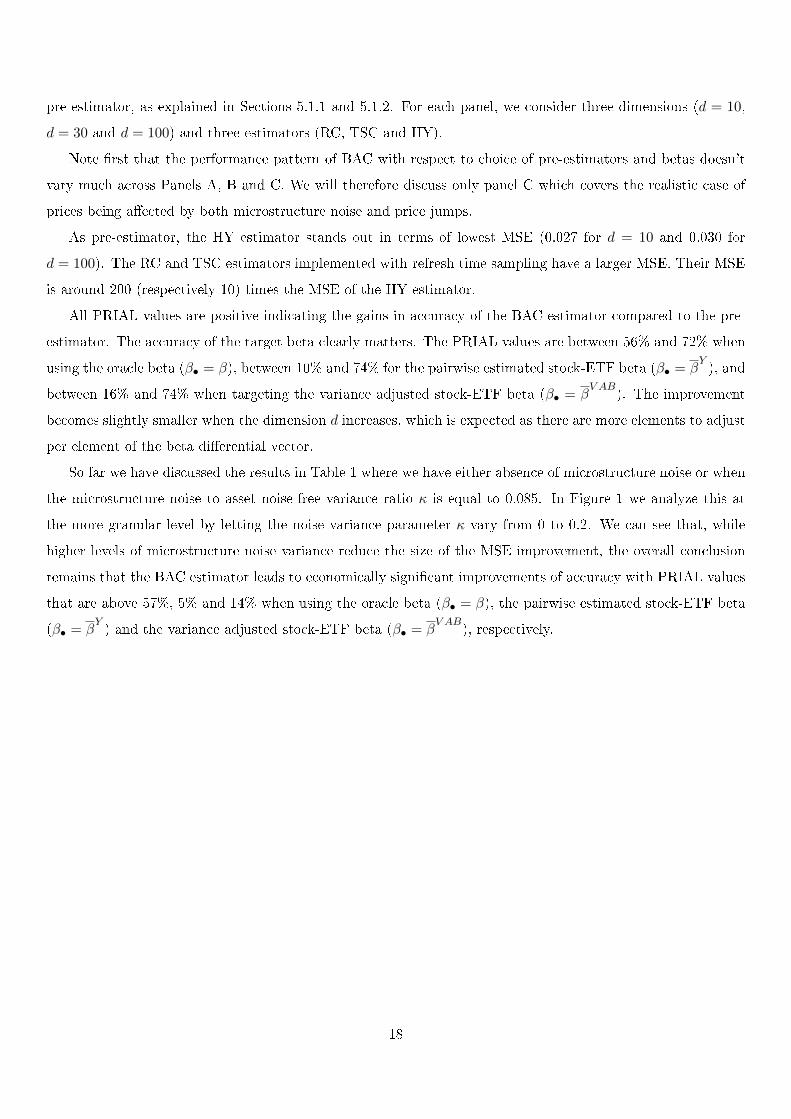
Note rst that the performance pattern of BAC with respect to choice of pre-estimators and betas doesn't
vary much across Panels A, B and C. We will therefore discuss only panel C which covers the realistic case of
prices being aected by both microstructure noise and price jumps.
As pre-estimator, the HY estimator stands out in terms of lowest MSE (0.027 for d = 10 and 0.030 for
d = 100). The RC and TSC estimators implemented with refresh time sampling have a larger MSE. Their MSE
is around 200 (respectively 10) times the MSE of the HY estimator.
All PRIAL values are positive indicating the gains in accuracy of the BAC estimator compared to the pre-
estimator. The accuracy of the target beta clearly matters. The PRIAL values are between 56% and 72% when
using the oracle beta (β• = β), between 10% and 74% for the pairwise estimated stock-ETF beta (β• = βY), and
between 16% and 74% when targeting the variance adjusted stock-ETF beta (β• = βV AB
). The improvement
becomes slightly smaller when the dimension d increases, which is expected as there are more elements to adjust
per element of the beta dierential vector.
So far we have discussed the results in Table 1 where we have either absence of microstructure noise or when
the microstructure noise to asset noise-free variance ratio κ is equal to 0.085. In Figure 1 we analyze this at
the more granular level by letting the noise variance parameter κ vary from 0 to 0.2. We can see that, while
higher levels of microstructure noise variance reduce the size of the MSE improvement, the overall conclusion
remains that the BAC estimator leads to economically signicant improvements of accuracy with PRIAL values
that are above 57%, 5% and 14% when using the oracle beta (β• = β), the pairwise estimated stock-ETF beta
(β• = βY) and the variance adjusted stock-ETF beta (β• = β
V AB), respectively.
18
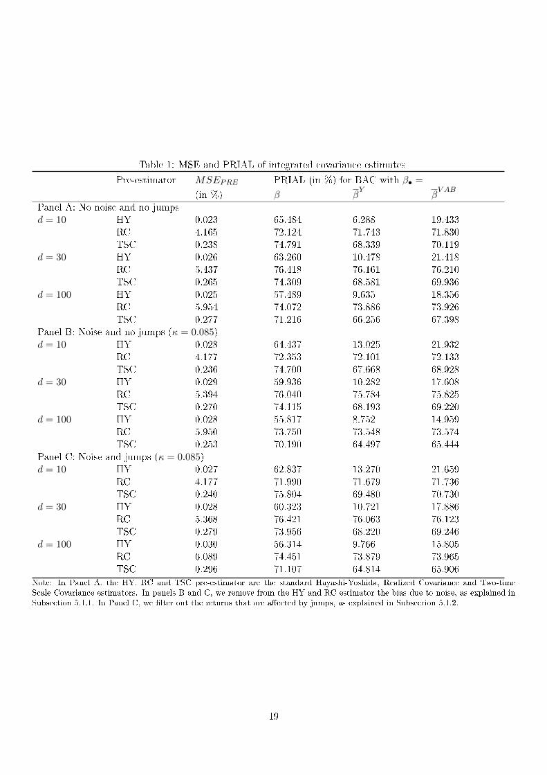
Table 1: MSE and PRIAL of integrated covariance estimates
Pre-estimator MSEPRE PRIAL (in %) for BAC with β• =
(in %) β βY
βV AB
Panel A: No noise and no jumpsd = 10 HY 0.023 65.484 6.288 19.433
RC 4.165 72.124 71.743 71.830TSC 0.238 74.791 68.339 70.119
d = 30 HY 0.026 63.260 10.478 21.418RC 5.437 76.418 76.161 76.210TSC 0.265 74.309 68.581 69.936
d = 100 HY 0.025 57.489 9.635 18.356RC 5.954 74.072 73.886 73.926TSC 0.277 71.216 66.256 67.398
Panel B: Noise and no jumps (κ = 0.085)d = 10 HY 0.028 64.437 13.025 21.932
RC 4.177 72.353 72.101 72.133TSC 0.236 74.700 67.668 68.928
d = 30 HY 0.029 59.936 10.282 17.608RC 5.394 76.040 75.784 75.825TSC 0.270 74.115 68.193 69.220
d = 100 HY 0.028 55.817 8.752 14.959RC 5.950 73.750 73.548 73.574TSC 0.253 70.190 64.497 65.444
Panel C: Noise and jumps (κ = 0.085)d = 10 HY 0.027 62.837 13.270 21.659
RC 4.177 71.990 71.679 71.736TSC 0.240 75.804 69.480 70.730
d = 30 HY 0.028 60.323 10.721 17.886RC 5.368 76.421 76.063 76.123TSC 0.279 73.956 68.220 69.246
d = 100 HY 0.030 56.314 9.766 15.805RC 6.089 74.451 73.879 73.965TSC 0.296 71.107 64.814 65.906
Note: In Panel A, the HY, RC and TSC pre-estimator are the standard Hayashi-Yoshida, Realized Covariance and Two-timeScale Covariance estimators. In panels B and C, we remove from the HY and RC estimator the bias due to noise, as explained inSubsection 5.1.1. In Panel C, we lter out the returns that are aected by jumps, as explained in Subsection 5.1.2.
19
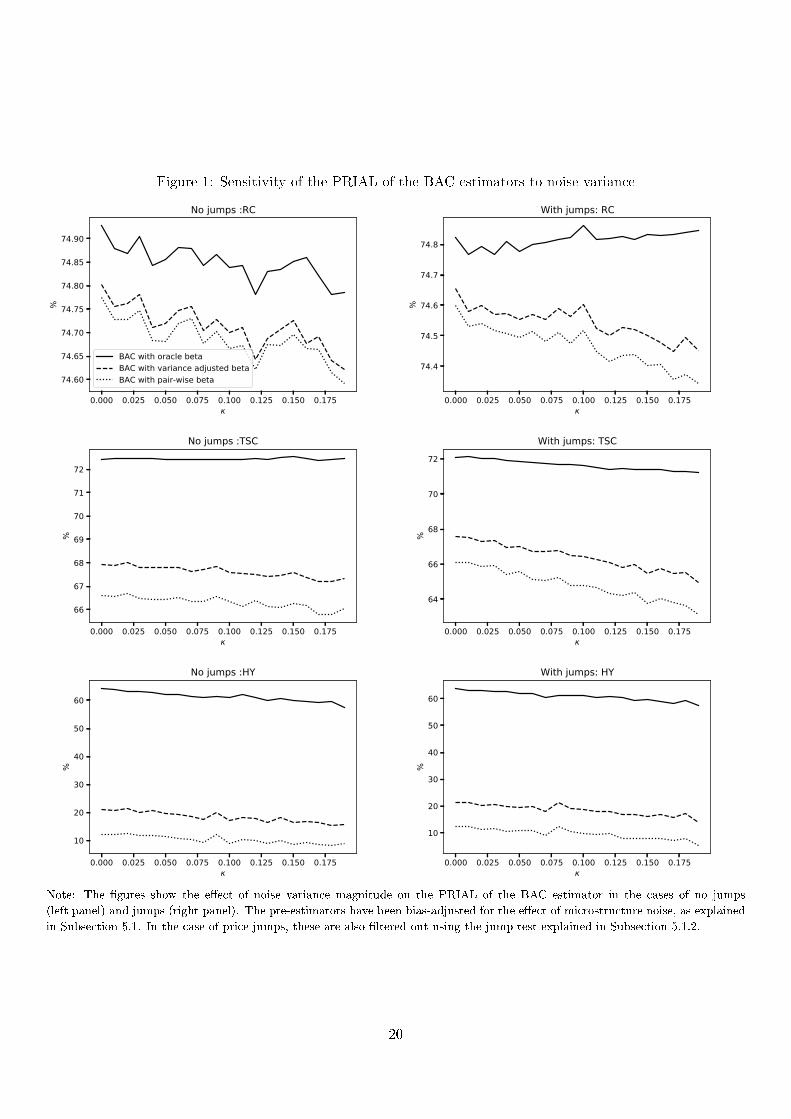
Figure 1: Sensitivity of the PRIAL of the BAC estimators to noise variance
0.000 0.025 0.050 0.075 0.100 0.125 0.150 0.175
74.60
74.65
74.70
74.75
74.80
74.85
74.90
%
No jumps :RC
BAC with oracle betaBAC with variance adjusted betaBAC with pair-wise beta
0.000 0.025 0.050 0.075 0.100 0.125 0.150 0.175
74.4
74.5
74.6
74.7
74.8
%
With jumps: RC
0.000 0.025 0.050 0.075 0.100 0.125 0.150 0.175
66
67
68
69
70
71
72
%
No jumps :TSC
0.000 0.025 0.050 0.075 0.100 0.125 0.150 0.175
64
66
68
70
72
%
With jumps: TSC
0.000 0.025 0.050 0.075 0.100 0.125 0.150 0.175
10
20
30
40
50
60
%
No jumps :HY
0.000 0.025 0.050 0.075 0.100 0.125 0.150 0.175
10
20
30
40
50
60
%
With jumps: HY
Note: The gures show the eect of noise variance magnitude on the PRIAL of the BAC estimator in the cases of no jumps
(left panel) and jumps (right panel). The pre-estimators have been bias-adjusted for the eect of microstructure noise, as explained
in Subsection 5.1. In the case of price jumps, these are also ltered out using the jump test explained in Subsection 5.1.2.
20
8 Empirical application
Our paper is motivated by the opportunity to improve realized covariance estimation by exploiting the increasing
number of transactions involving exchange traded funds. In this section, we document the BAC adjustment for
realized covariance estimation of the stocks for which the market capitalization weighted value is tracked by the
Financial Select Sector SPDR Fund, with ticker XLF. The Financial Select Sector SPDR Fund (XLF) is among
the most frequently traded ETFs (nasdaq.com, 2019).
We rst describe the data and compare the properties of the ETF data and the stock price data. Second, we
quantify the magnitude of the BAC adjustment and document its heterogeneity across time and stocks. Third,
we show that the adjustment improves the performance of an index tracking investor aiming at tracking the
XLF index with a small number of stocks.
8.1 Data
We use two years - from Jan 2 2018 to Dec 31, 2019 - of transaction prices from the Trades and Quotes (TAQ)
Millisecond database for the XLF fund transaction prices and its 67-69 components. The amount of investment
in the various assets is taken from the CRSP Mutual Funds constituents database. Data cleaning is performed
according to recommendations in Barndor-Nielsen et al. (2009). We nd that, for our sample, the XLF ETF
tracks the value of a market capitalization weighted portfolio invested in nancial sector stocks included in
the S&P 500 with a tight tracking error. We refer to citetpetajisto2017ineciencies for more dicusion on the
mechanism of shares redemption and the activity of arbitrageurs ensuring such low tracking errors.
Figure 2 reports the daily average number of cleaned trades for all stocks included in the XLF. It varies
between 1987 and 26038 observations per day with a an average (resp. median) value of 7330 (resp. 6091) trades
per day. The XLF fund itself has an average frequency of 12211 trades per day. Only eight stocks have a higher
number of observations, namely JPMorgan Chase (JPM), Bank of America (BAC), Citigroup (C), Wells Fargo
(WFC), Fifth Third Bancorp (FITB), Morgan Stanley (MS), Huntington Bancshares (HBAN) and E*TRADE
Financial Corporation (ETFC).
One exception is that for each stock we take all trades on the two most liquid exchanges instead of only one exchange. Thismodication substantially increases the number of observations with only little eect on the microstructure noise variance.
On our sample, the relative mispricing between the ETF price (exp(Yt)) and the weighted average of the most componentstock prices obtained using last tick interpolation for every minute. We nd that the relative mispricing is economically small. Itranges between -0.19% and 0.34%, with zero mean and median and standard deviation of 0.01% .
21
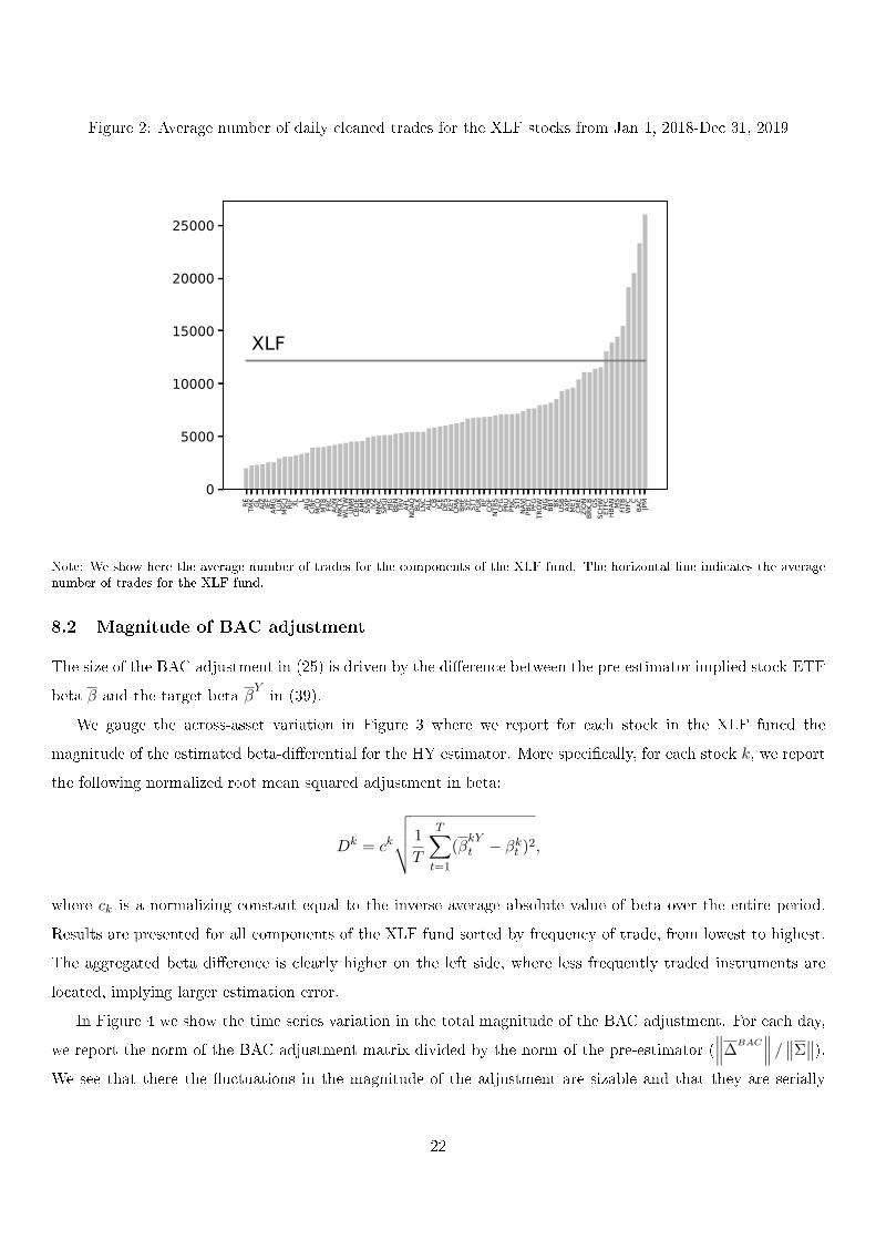
Figure 2: Average number of daily cleaned trades for the XLF stocks from Jan 1, 2018-Dec 31, 2019
RE TMK GL AIZ JEF
AMG
LUK
MSC
IRJ
F XL LAJ
GCI
NFM
CO MTB FR
CAO
NM
KTX
WLT
WUN
MCB
OE AMP
SIVB IV
ZM
MC
SPGI HIG
BEN
TRV
AFL
NDAQ BL
KLN
CAL
L CB ICE
DFS
KEY
CMA
BHF
SYF
STT
PGR RF COF
NTRS CFG
PRU
PNC STI
NAVI
PBCT PFG
TROW AI
GBB
T BK USB
AXP
MET
CME
ZION
BRK.
B GSSC
HW ETFC
HBAN M
SFI
TBW
FC CBA
CJP
M
0
5000
10000
15000
20000
25000
XLF
Note: We show here the average number of trades for the components of the XLF fund. The horizontal line indicates the averagenumber of trades for the XLF fund.
8.2 Magnitude of BAC adjustment
The size of the BAC adjustment in (25) is driven by the dierence between the pre-estimator implied stock-ETF
beta β and the target beta βYin (39).
We gauge the across-asset variation in Figure 3 where we report for each stock in the XLF funcd the
magnitude of the estimated beta-dierential for the HY estimator. More specically, for each stock k, we report
the following normalized root mean squared adjustment in beta:
Dk = ck
√√√√ 1
T
T∑t=1
(βkYt − βkt )2,
where ck is a normalizing constant equal to the inverse average absolute value of beta over the entire period.
Results are presented for all components of the XLF fund sorted by frequency of trade, from lowest to highest.
The aggregated beta dierence is clearly higher on the left side, where less frequently traded instruments are
located, implying larger estimation error.
In Figure 4 we show the time series variation in the total magnitude of the BAC adjustment. For each day,
we report the norm of the BAC adjustment matrix divided by the norm of the pre-estimator (∥∥∥∆
BAC∥∥∥ /∥∥Σ
∥∥).We see that there the uctuations in the magnitude of the adjustment are sizable and that they are serially
22
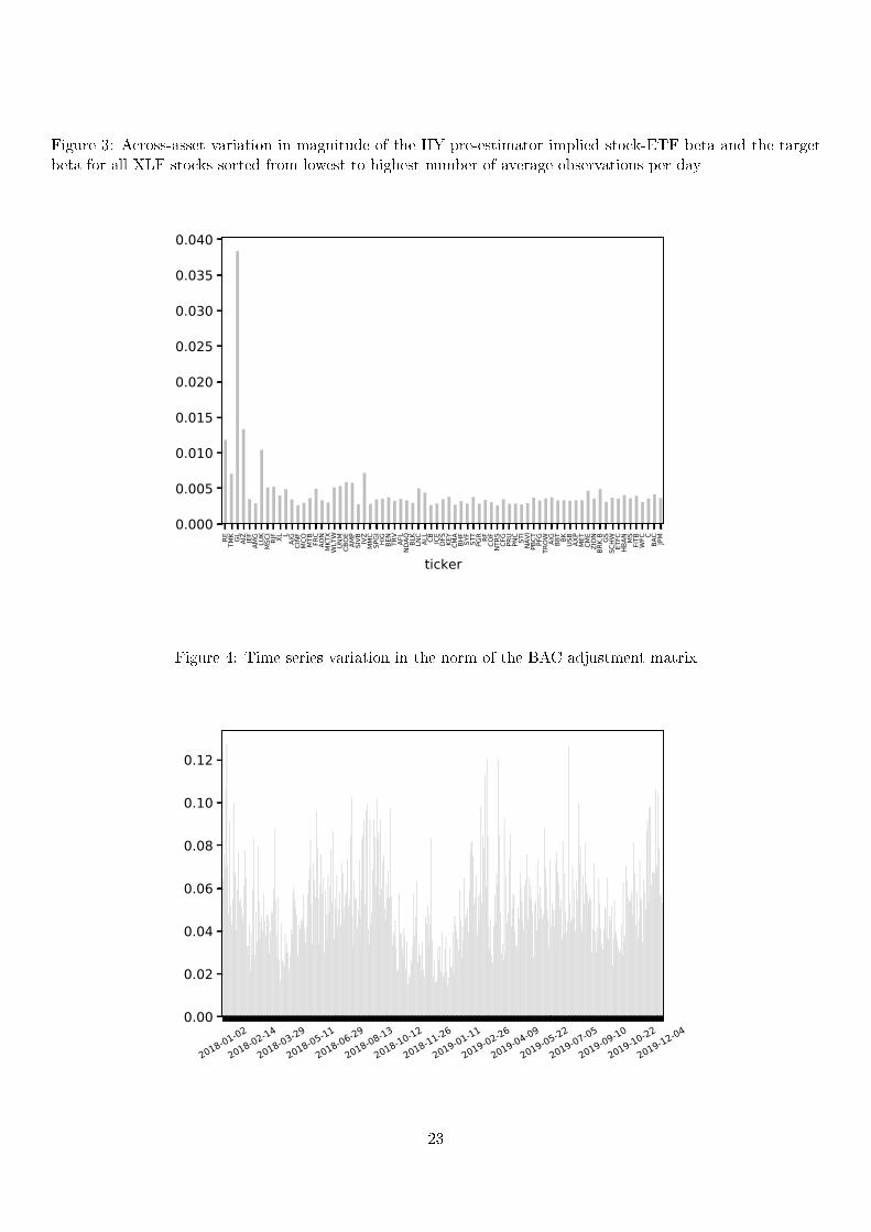
Figure 3: Across-asset variation in magnitude of the HY pre-estimator implied stock-ETF beta and the targetbeta for all XLF stocks sorted from lowest to highest number of average observations per day
RE TMK GL AIZ JEF
AMG
LUK
MSC
IRJ
F XL LAJ
GCI
NFM
CO MTB FR
CAO
NM
KTX
WLT
WUN
MCB
OE AMP
SIVB IV
ZM
MC
SPGI HIG
BEN
TRV
AFL
NDAQ BL
KLN
CAL
L CB ICE
DFS
KEY
CMA
BHF
SYF
STT
PGR RF COF
NTRS CFG
PRU
PNC STI
NAVI
PBCT PFG
TROW AI
GBB
T BK USB
AXP
MET
CME
ZION
BRK.
B GSSC
HW ETFC
HBAN M
SFI
TBW
FC CBA
CJP
M
ticker
0.000
0.005
0.010
0.015
0.020
0.025
0.030
0.035
0.040
Figure 4: Time series variation in the norm of the BAC adjustment matrix
2018-01-02
2018-02-14
2018-03-29
2018-05-11
2018-06-29
2018-08-13
2018-10-12
2018-11-26
2019-01-11
2019-02-26
2019-04-09
2019-05-22
2019-07-05
2019-09-10
2019-10-22
2019-12-040.00
0.02
0.04
0.06
0.08
0.10
0.12
23
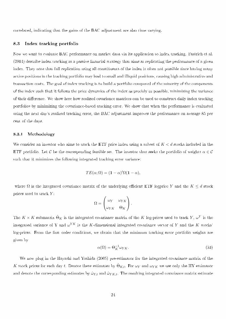
correlated, indicating that the gains of the BAC adjustment are also time-varying.
8.3 Index tracking portfolio
Now we want to evaluate BAC performance on market data via its application to index tracking. Fastrich et al.
(2014) describe index tracking as a passive nancial strategy that aims at replicating the performance of a given
index. They note that full replication using all constituents of the index is often not possible since having many
active positions in the tracking portfolio may lead to small and illiquid positions, causing high administrative and
transaction costs. The goal of index tracking is to build a portfolio composed of the minority of the components
of the index such that it follows the price dynamics of the index as precisly as possible, minimizing the variance
of their dierence. We show here how realized covariance matrices can be used to construct daily index tracking
portfolios by minimizing the covariance-based tracking error. We show that when the performance is evaluated
using the next day's realized tracking error, the BAC adjustment improves the performance on average 85 per
cent of the days.
8.3.1 Methodology
We consider an investor who aims to track the ETF price index using a subset of K < d stocks included in the
ETF portfolio. Let C be the corresponding feasible set. The investor thus seeks the portfolio of weights α ∈ C
such that it minimizes the following integrated tracking error variance:
TE(α; Ω) = (1− α)′Ω(1− α),
where Ω is the integrated covariance matrix of the underlying ecient ETF logprice Y and the K ≤ d stock
prices used to track Y :
Ω =
ωY ωY K
ωY K ΘK
.
The K ×K submatrix ΘK is the integrated covariance matrix of the K log-prices used to track Y , ωY is the
integrated variance of Y and ωY K is the K-dimensional integrated covariance vector of Y and the K stocks'
log-prices. From the rst order conditions, we obtain that the minimum tracking error portfolio weights are
given by
α(Ω) = Θ−1K ωY K . (53)
We now plug in the Hayashi and Yoshida (2005) pre-estimator for the integrated covariance matrix of the
K stock prices for each day t. Denote these estimates by ΘK,t. For ωY and ωY K we use only the HY estimator
and denote the corresponding estimates by ωY,t and ωY K,t. The resulting integrated covariance matrix estimate
24
is:
Ωt =
ωY,t ωY K,t
ωY K,t ΘK,t
.
The corresponding estimated minimum tracking error portfolio is α(Ωt).¶ We do the same for the BAC adjusted
pre-estimator leading to α(ΩBACt ).
In order to evaluate the tracking error performance of portfolio α(Ωt) we use the next day's covariance
estimate Ωt+1. The next days's tracking error is:
TEt+1(α(Ωt)) = ωY,t+1 − 2ωY K,tΘ−1K,tωY K,t+1 + ωY K,tΘ
−1K,tΘK,t+1Θ−1
K,tωY K,t.
If ΘK,t = ΘK,t+1, then α(Ωi) delivers the optimal portfolio by construction. We further create for each day
N = 10000 random sets of K stocks used in the index tracking. We sample K from a uniform distribution
between 10 and 30. For each day t, we then compute the percentage of subsets for which the BAC adjustment
has improved the tracking error:
Gt =1
N
N∑i=1
I(TEt+1(α(Ωt,i))−TEt+1(α(ΩBACt,i )))>0, (54)
where the portfolio weights are computed using estimators ΩHYt,i and ΩBAC
t,i of the previous day and the per-
formance is evaluated using the tracking error computed using Ωt+1,i of the day t+ 1. The latter is computed
using the 1-minute realized covariance as well as the Hayashi-Yoshida covariance estimator using all trades.
8.3.2 Results
We now use the next day's realized covariance to evaluate the gains obtained using the BAC estimator in
terms of achieving a low tracking error portfolio. The evaluation period ranges from Jan 1, 2018 to Dec 31,
2019. Excluding dates with missing data and dates of re-balancing, we have in total 442 days. The results are
presented in Figure 5, where we plot the 10-day moving averages for both pairs of estimators, comparing BAC
HY against HY and variance adjusted BAC HY against HY .
In the top plot, we can see that the BAC estimator outperforms the pre-estimator every day for over 84%
of the random subsets considered when we use the next day's HY estimator to evaluate the trackingerror. In
the bottom plot, we can see that if we use the variance adjusted beta as target beta, the outperformance of the
BAC estimator remains but is less outspoken. However, if we gauge the performance based on the next day's
1-minute realized covariance, then the BAC estimator with variance adjusted beta as target beta outperforms
perfoms simiilarly as the BAC estimator with the pairwise estimate as target beta.
¶When the pre-estimator or its BAC adjustment is not positive denite, we perform a spectral decomposition based regularizationas in Aït-Sahalia et al. (2010) and Fan et al. (2012).
25
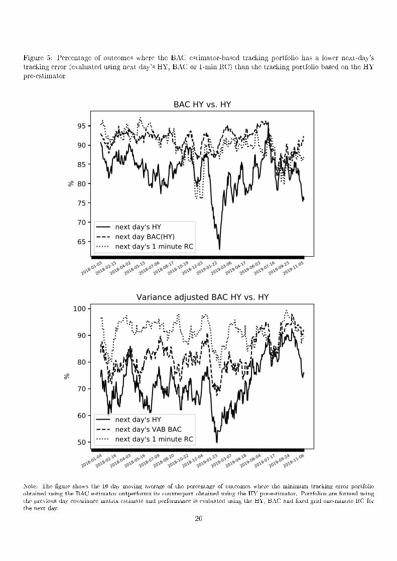
Figure 5: Percentage of outcomes where the BAC estimator-based tracking portfolio has a lower next-day'stracking error (evaluated using next day's HY, BAC or 1-min RC) than the tracking portfolio based on the HYpre-estimator
2018-01-03
2018-02-15
2018-04-02
2018-05-15
2018-07-06
2018-08-17
2018-10-19
2018-12-03
2019-01-22
2019-03-06
2019-04-17
2019-06-03
2019-07-16
2019-09-23
2019-11-05
65
70
75
80
85
90
95
%
BAC HY vs. HY
next day's HYnext day BAC(HY)next day's 1 minute RC
2018-01-04
2018-02-16
2018-04-03
2018-05-16
2018-07-09
2018-08-20
2018-10-22
2018-12-04
2019-01-23
2019-03-07
2019-04-18
2019-06-04
2019-07-17
2019-09-24
2019-11-06
50
60
70
80
90
100
%
Variance adjusted BAC HY vs. HY
next day's HYnext day's VAB BACnext day's 1 minute RC
Note: The gure shows the 10-day moving average of the percentage of outcomes where the minimum tracking error portfolioobtained using the BAC estimator outperforms its counterpart obtained using the HY pre-estimator. Portfolios are formed usingthe previous day covariance matrix estimate and performance is evaluated using the HY, BAC and xed grid one-minute RC forthe next day.
26
While it remains a topic for further research to obtain even better estimates for the stock-ETF beta (and
possibly exploit expert opinion), we can conclude from the empirical analysis that the BAC adjustment with
the pairwise stock-ETF beta yields improved minimum variance tracking error portfolio in the vast majority of
the random subsets considered.
9 Conclusion
Over the past decade, the trading frequency of several Exchange Traded Funds (ETFs) has surpassed the
frequency at which many of their component stocks trade. In this paper, we show that this trend has a positive
spillover eect in terms of improved covariance estimation of the underlying stock returns. We develop an
econometric framework to exploit the information value in the highfrequency comovement between stock and
ETF prices for the estimation of the covariation between stock prices over a xed time interval.
The proposed Beta Adjusted Covariance estimator improves a pre-estimator in such a way that the implied
stock-ETF beta equals a target value. The latter can either be based on pairwise estimation using stock and ETF
prices or be dened using expert opinion. We develop the asymptotic theory for the stock-ETF beta associated
to the Hayashi and Yoshida (2005) pre-estimator. In the simulation study, we show that the accuracy gains
are over 50% in the case in which the target value for the stock-ETF beta is set by an expert to the oracle
beta that is assumed to be free from estimation error. The accuracy gains remain economically signicant
when the target beta is estimated using ETF prices and stock prices. The empirical application on Trades and
Quotes millisecond transaction data demonstrates the usefulness of the BAC adjustment for an investor aiming
at tracking an investment index with a small number of stocks.
To help practitioners and academics to implement our methodology in practice, we have included the open
source implementation of the BAC estimator in the R package highfrequency (Boudt et al., 2021) and the
Python package bacpack (Dragun et al., 2021).
27

10 Appendix 1: Derivation of the BAC estimator
10.1 Example of Q matrix
The nd-dimensional vector δ corresponds to the adjustment to the n spot covariances estimated using the pre-
estimator. We use the d(d − 1)/2 × dn matrix Q to make sure that symmetry in the adjusted covariance is
guaranteed by imposing Qδ = 0d(d−1)/2. To illustrate this, suppose that d = 2. In this situation, we require
that ∆12 = ∆21 which, is equivalent to having that
n2∑l=1
δ12l =
n1∑l=1
δ21l .
Since Q =[0′n1
1′n2−1′n1
0′n2
], it follows that
Qδ =
n2∑l=1
δ12l −
n1∑l=1
δ21l .
We conclude easily from this that ∆12 = ∆21 if and only if Qδ = 0.
10.2 Proof of Equation (22)
Let us start by considering the Lagrangian corresponding to the optimization problem (18). Plainly,
L = δ′Pδ −[(W ′, Q′)′δ −
((β − β•)′, 0′(d−1)d/2
)′]′λ,
with λ as the vector of Lagrange multipliers. Thus, the n =∑d
k=1 nk rst order conditions for the elements of
δ are:∂L∂δ
= 2Pδ − (W ′, Q′)λ = 0n. (55)
For the d× 1 Lagrangian multipliers λi, we have:
∂L∂λ
= (W ′, Q′)′δ −(
(β − β•)′, 0′(d−1)d/2
)′= 0d. (56)
From (55) and (56) we obtain:
(W ′, Q′)′P−1(W ′, Q′)λ = 2(
(β − β•)′, 0′(d−1)d/2
)′.
Applying the previous relation to (56) and using standard formulas for the inverse of block matrices, we get
that δ equals
28

P−1
D −DWP−1Q′(QP−1Q′
)−1
−(QP−1Q′
)−1QP−1W ′D
(QP−1Q′
)−1+(QP−1Q′
)−1QP−1W ′DWP−1Q′
(QP−1Q′
)−1
×
β − β•0(d−1)d/2
where
D =(WP−1W ′ −WP−1Q′
(QP−1Q′
)−1QP−1W ′
)−1.
Therefore,
vec(∆) = AP−1
WQ
′ D
−(QP−1Q′
)−1QP−1W ′D
P−1
WQ
′ D
−(QP−1Q′
)−1QP−1W ′D
(β − β•)= AP−1
(I −Q′
(QP−1Q′
)−1QP−1
)W ′D
(β − β•
).
Thus, it only remains to show that
L = AP−1(I −Q′
(QP−1Q′
)−1QP−1
)W ′(WP−1W ′ −WP−1Q′
(QP−1Q′
)−1QP−1W ′
)−1, (57)
with L as in (23). To do this, observe rst that
QP−1Q′ = 2Id2 ; AP−1W ′ = W ′. (58)
Indeed, by using the denition of Q, it is easy to see that
(QQ′
) (i−2)(i−1)2
+j,(i′−2)(i′−1)
2+j′
=1
ni
(j−1)n+∑i
k=1 nk∑l=(j−1)n+
∑i−1k=1 nk+1
Q(i′−2)(i′−1)
2+j′,l
− 1
nj
(i−1)n+∑j
k=1 nk∑l=(i−1)n+
∑j−1k=1 nk+1
Q(i′−2)(i′−1)
2+j′,l
=(αii′αjj
′ − αij′αji′)− (αij′αji′ − αii′αjj′)
for all i, j, i′, j′ = 1, . . . , d, i > j, i′ > j′. Note that if i = j′ and j = i′, we would have that j > i, which is
absurd. Therefore,
(QQ′
) (i−2)(i−1)2
+j,(i′−2)(i′−1)
2+j′
= 2αii′αjj
′= 2I
(i−2)(i−1)2
+j,(i′−2)(i′−1)
2+j′
d2 .
29

Similar arguments can be used to deduce that for all m, r, j = 1, . . . , d
nd∑l=1
(1/P ll)A(m−1)d+r,lW k,l =1
nr
(m−1)n+∑r
x=1 nx∑l=(m−1)n+
∑r−1x=1 nx+1
W k,l
=αmk
nr
nr∑m=1
wrtrm−1= W k,(m−1)d+r,
which shows the validity of (58). Applying the latter to the right-hand side of (57) allows us to conclude that
(22) holds if and only if
L =
(W ′ − 1
2AP−1Q′QP−1W ′
)(WP−1W ′ − 1
2WP−1Q′QP−1W ′
)−1
. (59)
Trivially, WP−1W ′ = Id2
(∑dy=1
1ny
∑ny
l=1(wytyl−1
)2). Moreover, in view that for all i, j, i′, j′, k,m, r = 1, . . . , d
with i > j and i′ > j′, it holds that
nd∑l=1
(1/P ll)A(m−1)d+r,lQ(i−2)(i−1)
2+j,l =
1
nr
(m−1)n+∑r
x=1 nx∑l=(m−1)n+
∑r−1x=1 nx+1
Q(i−2)(i−1)
2+j,l
= αmjαri − αmiαrj ,
(60)
and
nd∑l=1
(1/P ll)Q(i−2)(i−1)
2+j,lW k,l =
1
ni
(j−1)n+∑i
x=1 nx∑l=(j−1)n+
∑i−1x=1 nx+1
W k,l − 1
nj
(i−1)n+∑j
x=1 nx∑l=(i−1)n+
∑j−1x=1 nx+1
W k,l
= αkj1
ni
ni∑l=1
witil−1− αki 1
nj
nj∑l=1
wjtjl−1
,
in which we have let αkl denote the Dirac's delta measure. We obtain that
(WAP−1Q′
)k, (i−2)(i−1)2
+j=
d∑m=1
(αmjαmk
1
ni
ni∑l=1
witil−1
)−
d∑m=1
(αmjαmi
1
nj
nj∑l=1
wjtjl−1
)
=(QP−1W ′
) (i−2)(i−1)2
+j,k.
Consequently, we can rewrite the right-hand side of (59) as
(Id2 −
1
2
(AP−1Q′
) (AP−1Q′
)′)W ′
Id2
d∑y=1
1
ny
ny∑l=1
(wytyl−1
)2
− 1
2W(AP−1Q′
) (AP−1Q′
)′W ′
−1
.
30

Therefore, in order to nish the proof, we only need to check that(AP−1Q′
) (AP−1Q′
)′= Q, where Q is as in
(21). From (60) we obtain that for all m, r,m′, r′ = 1, . . . , d
[(AP−1Q′
) (AP−1Q′
)′](m−1)d+r,(m′−1)d+r′
=
d−1∑j=1
d∑i=j+1
(αmjαri − αmiαrj)(αm′jαr′i − αm′iαr′j),
which obviously vanishes when m = r. Suppose that m > r. Then,
[(AP−1Q′
) (AP−1Q′
)′](m−1)d+r,(m′−1)d+r′
=d∑
i=r+1
αmi(αm′iαr
′r − αm′rαr′i)
= αm′mαr
′r − αm′rαr′m
= Q(m−1)d+r,(m′−1)d+r′ .
Interchanging the roles between r and m above, we obtain the desired relation(AP−1Q′
) (AP−1Q′
)′= Q,
which completes our argument.
10.3 Proof of Proposition 3
First note that from Itô's lemma
d exp(Xks ) = exp(Xk
s )(dXs +1
2d[Xk]s)
d exp(Y ∗s ) = exp(Y ∗s )(dY ∗s +1
2d[Y ∗]s),
and exp(Y ∗s ) =∑d
k=1 aks exp(Xk
s ) =∑d
k=1wks . It thus follows that under the assumptions of Section 2, we have
that
dY ∗s =1
exp(Y ∗s )
d∑k=1
wks
(dXk
s +1
2d[Xk]s
)− 1
2d[Y ∗]s (61)
[X l, Y ∗]t =d∑
k=1
∫ t
0
wksexp(Y ∗s )
d[Xk, X l]s. (62)
For the weighted sum of betasd∑l=1
wlsexp(2Y ∗s )
dβls, (63)
with βls as dened in (41) we have that from (62) the following result follows:
d∑l=1
wlsexp(2Y ∗s )
dβls =d∑l=1
wlsexp(Y ∗s )
d∑k=1
wksexp(Y ∗s )
d[Xk, X l]s =d∑l=1
wlsexp(Y ∗s )
d[Y ∗, X l]s = d[Y ∗]s.
31

11 Appendix 2: Asymptotics for stochastic functionals of a localized HY
estimator
Consider kn ∈ N a window satisfying that kn ↑ ∞ and kn/n→ 0, as n→∞ for a given Itô's semimartingale H
with representation
Ht =H0 +
∫ t
0µ′sds+
d′∑m=1
∫ t
0σ′ms dBm
s
+
∫ t
0
∫Eϕ′(s, z)1‖ϕ′(s,z)‖≤1(N − λ)(dsdz) +
∫ t
0
∫Eϕ′(s, z)1‖ϕ′(s,z)‖>1N(dsdz),
(64)
in which µ′, σ′ and δ′ satisfy the same assumptions as µ, σ and δ in (3). Within this framework, we dene
ψkl(H) =
∫ 1
0HsΣ
kls ds
and
ψkln (H) =1
nk
nk−kn+1∑m=1
Htkm−1Σkltkm−1
, (65)
where
Σkltkm
=nkkn
Σkltkm+kn/nk
− Σkltkm
, m = 0, 1, . . . , nk − kn. (66)
For H(1), . . . ,H(N) processes of the form of (64) we use the notation
Λ(H(1), . . . ,H(m)) = (ψkln (H(1))− ψkl(H(1)), . . . , ψkln (H(N))− ψkl(H(N)))k,l=1,...,d.
We have the following result:
Theorem 2. Assume that X is given by (1) and let Assumption 1 hold. If k2n/n→ 0, then as n→∞
√nΛ(H(1), . . . ,H(m))
s.d→ Z = (Zkl1 , . . . , ZklN )k,l=1,...,d,
in which Z is an F-conditional centered Gaussian vector satisfying
E(Zklx , Z
k′,l′y
∣∣∣F) =
∫ 1
0H(x)s H(y)
s
(Σk,k′s Σl,l′
s +Σkl′s Σk′,l
s
)ds.
Remark 2. Thanks to Lemma 4.4.9 in Jacod and Protter (2011), in all the proofs below we may and do assume
32

that σ, µ, σ, µ, µ′, σ′ and X are bounded as well as
‖ϕ(ω, t, z)‖+∥∥ϕ′(ω, t, z)∥∥ ≤ Γ (z),
where Γ is a deterministic bounded measurable function fullling that∫E Γ (z)2ν(dz) < ∞. Under these strong
assumptions, we have that
Ht = H0 +
∫ t
0µ′sds+
d′∑m=1
∫ t
0σ′ms dBm
s +
∫ t
0
∫Eϕ′(s, z)(N − λ)(dsdz),
where µ′ is bounded. Moreover, for all s ≥ 0 and p ≥ 1
E(
supu≤s‖Xt+u −Xt‖p
∣∣∣∣Ft) ≤ Csp/2‖E (Xt+s −Xt| Fs)‖ ≤ Cs,
E(
supu≤s|Σt+u −Σt|p
∣∣∣∣Ft) ≤ Cs1∧p/2,
‖E (Σt+s −Σt| Fs)‖ ≤ Cs,
E(
supu≤s|Ht+u −Ht|p
∣∣∣∣Ft) ≤ Cs1∧p/2,
‖E (Ht+s −Ht| Fs)‖ ≤ Cs.
(67)
For more details in this regard we refer to Section 2 in Jacod and Protter (2011).
11.1 First approximation
For the remainder of this work, if Z and Y denote two stochastic processes, we will write
βklp (Y,Z) =∑i,j
∆i,kY∆j,lZ1(tkp−1,tkp ](t
ki ∨ tlj)1Iki ∩Ilj 6=∅;
βklm(Y,Z) =∑i,j
∆i,kY∆j,lZ1(m−1n
,mn
](tki ∨ tlj)1Iki ∩Ilj 6=∅,
(68)
for k = 1, . . . , d, l = 1, . . . , d′, p = 1, . . . , nk − 1 and m = 1, . . . , n. Note that
ψkl(H) =
nk∑p=1
hp,nβklp (Xk, X l),
where
hp,n =1
kn
p∧(nk−kn+1)∑m=1∨(p−kn+1)
Htkm−1.
33
For the rest of this part we focus on showing the following approximation:
Lemma 1. Assume that X and H are given by (1) and (64), respectively. Let Assumption 1 hold and suppose
that k2n/n→ 0. Then,
ψkl(H) =
nk∑p=1
Htkpβklp (Xk, X l) + oP(n−1/2)
=∑i,j
Htki−1∧tlj−1∆i,kX
k∆j,lXl1Iki ∩Ilj 6=∅
+ oP(n−1/2)
=n∑
m=1
Hm−1nβklm(Xk, X l) + oP(n−1/2).
(69)
Proof. We will only show the rst equality in (69). The other approximations can be shown using the same
method. For n suciently large, dene the error of the rst approximation by
Rn,1 =
nk∑p=1
(hp,n −Htkp
)βklp (Xk, X l).
In view that Iki ∩ I lj 6= ∅ if and only if the following four scenarios occur
tki ≥ tlj ≥ tki−1 and tki−1 ≥ tlj−1
tlj ≥ tki ≥ tlj−1 and tki−1 ≥ tlj−1
tki ≥ tlj ≥ tki−1 and tlj−1 ≥ tki−1
tlj ≥ tki ≥ tlj−1 and tlj−1 ≥ tki−1
, (70)
we deduce, from Assumption 1, the estimates in (67), Jensen's inequality and the Cauchy-Schwarz inequality
that for all J ≥ 1
E(∣∣∣βklp (Xk, X l)
∣∣∣J) ≤ C/nJ , p = 1, . . . , nk. (71)
Thus, letting ln = kn/nk and using once again the Cauchy-Schwarz inequality, we obtain that
kn∑p=1
E(∣∣∣(hp,n −Htkp
)βklp (Xk, X l)
∣∣∣) ≤ Cnk
kn∑p=1
E
∣∣∣∣∣Htkp− 1
kn
p∑m=1
Htkm−1
∣∣∣∣∣21/2
=C
∫ ln
0E
∣∣∣∣∣H [snk]+1
nk
− 1
ln
∫ [snk]+1
nk
0H [rnk]
nk
dr
∣∣∣∣∣21/2
ds
=Cln
∫ 1
0E
∣∣∣∣∣H [hnrnk]
nk
−∫ [snk]+1
nkhn
0H [hnsnk]
nk
ds
∣∣∣∣∣21/2
dr ≤ Cln.
34
Similar calculations show that
nk∑p=nk−kn+1
E(∣∣∣(hp,n −Htkp
)βklp (Xk, X l)
∣∣∣) ≤ Cln.Thus, using that
√nln → 0, we conclude that
Rn,1 =1
kn
nk−2kn∑q=kn+1
∆q,kH
q+kn−1∑p=q
βklp (Xk, X l)(q − p+ kn)
+1
kn
kn∑q=1
∆q,kH
q+kn−1∑p=kn
βklp (Xk, X l)(q − p+ kn)
+1
kn
nk−kn−1∑q=nk−2kn+1
∆q,kH
nk−kn∑p=q
βklp (Xk, X l)(q − p+ kn) + oP(n−1/2).
Furthermore, in view thatq+kn−1∑p=q
(q − p+ kn) = O(k2n), q = 1, . . . , nk − kn, (72)
we can apply (71) to deduce that
Rn,1 =1
kn
nk−2kn∑q=kn+1
∆q,kH
q+kn−1∑p=q
βklp (Xk, X l)(q − p+ kn) + oP(n−1/2). (73)
Now, let Ar be the set of indexes (i, j) satisfying the rth scenario in (70), put
βklp,r(Xk, X l) =
∑i,j∈Ar
∆i,kXk∆j,lX
l1(tkp−1,tkp ](t
ki ∨ tlj)1Iki ∩Ilj 6=∅
and dene
Un,1(r) =
√n
kn
nk−2kn∑q=kn+1
q+kn−1∑p=q+1
∆q,kHβklp,r(X
k, X l)(q − p+ kn);
Un,1(r) =√n
nk−2kn∑q=kn+1
∆q,kHβklq,r(X
k, X l).
Since√nRn,1 =
∑4r=1
(Un,1(r) + Un,1(r)
), we need to show that Un,1(r) and Un,1(r) are asymptotically negli-
gible for r = 1, 2, 3, 4. We will only show the case for r = 1. By Jensen's inequality and Lemma 2.2.12 in Jacod
35

and Protter (2011), we need to show that
mn,U =
√n
kn
nk−2kn∑q=kn+1
q+kn−1∑p=q+1
E(
∆q,kHβklp,1(Xk, X l)
∣∣∣Ftkq−1
)(q − p+ kn) = oP(1),
mn,U =√n
nk−2kn∑q=kn+1
E(
∆q,kHβklq,1(Xk, X l)
∣∣∣Ftkq−1
)= oP(1)
(74)
and
vn,U =n
k2n
nk−2kn∑q=kn+1
E
∆q,kH
q+kn−1∑p=q+1
βklp,1(Xk, X l)(q − p+ kn)
2∣∣∣∣∣∣Ftkq−1
= oP(1),
vn,U = n
nk−2kn∑q=kn+1
E[(
∆q,kHβklq,1(Xk, X l)
)2∣∣∣∣Ftkq−1
]= oP(1).
(75)
From Remark 2 and Itô's formula, we have that for any t ≥ s ≥ u and k, l = 1, . . . , d
E[
(Ht −Hs)(Xkt −Xk
s
)∣∣∣Fu] =E[∫ t
s(Hr −Hs)µ
krdr
∣∣∣∣Fu]+ E[∫ t
s(Xk
r −Xks )µ′rdr
∣∣∣∣Fu]+ E
[∫ t
sϕ(1)r dr
∣∣∣∣Fu] . (76)
We also have that
E[
(Ht −Hs)(Xkt −Xk
s
)(X lt −X l
s
)∣∣∣Fu] =E[∫ t
s(Hr −Hs)
(Xkr −Xk
s
)µlrdr
∣∣∣∣Fu]+ E
[∫ t
s(Hr −Hs)
(X lr −X l
s
)µkrdr
∣∣∣∣Fu]+ E
[∫ t
s
(Xkr −Xk
s
)(X lr −X l
s
)µ′rdr
∣∣∣∣Fu]+ E
[∫ t
s
(Xkr −Xk
s
)ϕ(2)r dr
∣∣∣∣Fu]+ E
[∫ t
s
(X lr −X l
s
)ϕ(1)r dr
∣∣∣∣Fu]+ E[∫ t
s(Hr −Hs)Σ
klr dr
∣∣∣∣Fu] ,(77)
for some càdlàg processes ϕ(1), ϕ(2) depending only on σ and σ′. Let q ∈ kn + 1, . . . , nk − 2kn. It follows from
(76), (77), Assumption 1 and (67) that if (p, j) ∈ A1 is such that tlj−1 ≥ tkq and p ≥ q + 1, we have as in (76)
that
∣∣∣E(∆p,kXk∆j,lX
l∣∣∣Ftkq)− (tlj − tkp−1)Σkl
tkq−1
∣∣∣ ≤ Cn−3/2, (78)
36

while for tkq ≥ tlj−1
E(
∆p,kXk∆j,lX
l∣∣∣Ftkq) =
(X ltkq−X l
tlj−1
)E(
∆p,kXk∣∣∣Ftkq)
+ E(
∆p,kXk(X ltlj−X l
tkq
)∣∣∣Ftkq)=(X ltkq−X l
tlj−1
)∫ tkp
tkp−1
E(µkr
∣∣∣Ftkq) dr+ (tlj − tkp−1)Σkl
tkq−1
+ OP(n−3/2).
We conclude that
E[∣∣∣E(∆q,kH∆p,kX
k∆j,lXl∣∣∣Ftkq−1
)− (tlj − tkp−1)Σkl
tkq−1E(
∆q,kH| Ftkq−1
)∣∣∣] ≤ Cn−2.
Therefore,
mn,U =
√n
kn
nk−2kn∑q=kn+1
q+kn−1∑p=q+1
∑j
(tlj − tkp−1)Σkltkq−1
E(
∆q,kH| Ftkq−1
)1(p,j)∈A1
(q − p+ kn) + oP(1) = oP(1),
where we have also used (72) and (67). To deal with mn,U rst note that
E(
∆q,kH∆q,kXk∆j,lX
l∣∣∣Ftkq−1
)=(X l
tkq−1−X l
tkj−1)× E
(∆q,kH∆q,kX
k∣∣∣Ftkq−1
)+ E
((Htlj−Htkq−1
)(Xktlj−Xk
tkq−1
)(X ltlj−X l
tkq−1
)∣∣∣Ftkq−1
)+ E
((Htkq−Htlj
)(Xktkj−Xk
tkq−1
)(X ltlj−X l
tkq−1
)∣∣∣Ftkq−1
)+ E
((Htlj−Htkq−1
)(Xktkq−Xk
tkj
)(X ltlj−X l
tkq−1
)∣∣∣Ftkq−1
)+ E
((Htkq−Htlj
)(Xktkq−Xk
tkj
)(X ltlj−X l
tkq−1
)∣∣∣Ftkq−1
)=OP(n−2) + E
[∫ tkq
tkq−1
(X ltkq−1−X l
tkj−1
)ϕ(1)r dr
∣∣∣∣∣Ftkq−1
]
+ E
[∫ tlj
tkq−1
(Xkr −Xk
tkq−1
)ϕ(2)r dr
∣∣∣∣∣Ftkq−1
]+ E
[∫ tkj
tkq−1
(X lr −X l
tkq−1
)ϕ(1)r dr
∣∣∣∣∣Ftkq−1
]
E
[∫ tkq
tlj
(X ltkj−X l
tkq−1
)ϕ(1)r dr
∣∣∣∣∣Ftkq−1
];
37
so
mn,U =√n
nk−2kn∑q=kn+1
∑j
E
[∫ tkq
tkq−1
(X ltkq−1−X l
tkj−1
)ϕ(1)r dr
∣∣∣∣∣Ftkq−1
]1(q,j)∈A1
+√n
nk−2kn∑q=kn+1
∑j
E
[∫ tlj
tkq−1
(Xkr −Xk
tkq−1
)ϕ(2)r dr
∣∣∣∣∣Ftkq−1
]1(q,j)∈A1
+√n
nk−2kn∑q=kn+1
E
[∫ tkj
tkq−1
(X lr −X l
tkq−1
)ϕ(1)r dr
∣∣∣∣∣Ftkq−1
]1(q,j)∈A1
+√n
nk−2kn∑q=kn+1
E
[∫ tkq
tlj
(X ltkj−X l
tkq−1
)ϕ(1)r dr
∣∣∣∣∣Ftkq−1
]1(q,j)∈A1
+ oP(1).
(79)
Since ϕ(1) is càdlàg, the Cauchy-Schwarz inequality and the Dominated Convergence Theorem guarantee that
the sum
√n
nk−2kn∑q=kn+1
∑j
E
∣∣∣∣∣E[∫ tkq
tkq−1
(X ltkq−1−X l
tkj−1
)(ϕ(1)r − ϕ
(1)
tkq−1
)dr
∣∣∣∣∣Ftkq−1
]∣∣∣∣∣1(q,j)∈A1
is bounded (up to a constant) by
nk−2kn∑q=kn+1
∫ tkq
tkq−1
E
(∥∥∥∥ϕ(1)r − ϕ
(1)
tkq−1
∥∥∥∥2)1/2
dr → 0. (80)
Consequently, the rst term in (79) equals
√n
nk−2kn∑q=kn+1
∑j
ϕ(1)
tkq−1
∫ tkq
tkq−1
E[(X ltkq−1−X l
tkj−1
)∣∣∣Ftkq−1
]dr1(q,j)∈A1
+ oP(1) = oP(1), (81)
thanks to (67). A similar argument can be applied to the other summands in (79) in order to deduce that (74)
is indeed true. Now we concentrate on showing that (75) is satised. Fix q ∈ kn + 1, . . . , nk − 2kn and pick
(p, j), (p′, j′) ∈ A1 such that q + kn − 1 ≥ p, p′ ≥ q + 1 and put
αklp,p′,j,j′(q) = E(
∆p,kXk∆p′,kX
k∆j,lXl∆j′,lX
l∣∣∣Ftkq) .
38

Suppose rst that j′ ≥ j. Then,
αklp,p′,j,j′(q) =
O(n2) if tlj−1 ≥ tkq ;(X ltkq−X l
tlj−1
)E(
∆p,kXk∆p′,kX
k∆j′,lXl∣∣Ftkq)+ O(n−2) if tlj′−1 ≥ tkq > tlj−1;(
X ltkq−X l
tlj−1
)(X ltkq−X l
tlj′−1
)E(
∆p,kXk∆p′,kX
k∣∣Ftkq)+ O(n−2) tkq > tlj′−1 ≥ tlj−1.
Moreover, thanks to (76) and (78), if tlj′−1 ≥ tkq > tlj−1,
∣∣∣E(∆p,kXk∆p′,kX
k∆j′,lXl∣∣∣Ftkq)∣∣∣ ≤
C/n2 if tkp > tkp′ or if t
lj′−1 ≥ tkp;
C/n3/2 tkp′ ≥ tkp > tlj′−1,
as well as ∣∣∣E(∆p,kXk∆p′,kX
k∣∣∣Ftkq)∣∣∣ ≤
C/n2 if p 6= p′;
C/n if p = p.
Hence, if j ≥ j′,
E∣∣∣E [(∆q,kH)2 ∆p,kX
k∆j,lXl∆p′,kX
k∆j′,lXl∣∣∣Ftkq−1
]∣∣∣ ≤ Cn−5/2,
whenever tlj′−1 ≥ tkq > tlj−1 and tkp′ ≥ tkp > tlj′−1 or when tkq > tlj′−1 ≥ tlj−1 and p 6= p′. Otherwise, we have that
E∣∣∣E [(∆q,kH)2 ∆p,kX
k∆j,lXl∆p′,kX
k∆j′,lXl∣∣∣Ftkq−1
]∣∣∣ ≤ Cn−3.
Interchanging j with j′ above and applying (72), we can conclude that
E (|vn,U |) ≤C1
n3/2
nk−2kn∑q=kn+1
q+kn−1∑p,p′=q+1
∑j′≥j
1tlj′−1≥tkq>tlj−1
1(p,j),(p′,j′)∈A11tk
p′≥tkp>t
lj′−1
+ o(1).
The rst part of (75) now follows from the fact that the last sum contains O(nkn) terms due to Assumption 1.
Finally, from the estimates in (67), the Cauchy-Schwarz inequality and (71) we obtain that
E[(
∆q,kHβklq,1(Xk, X l)
)2]≤ C/n5/2,
which trivially implies that vn,U is negligible as n→∞. This concludes our argument.
39

11.2 Negligibility of the drift component
From Lemma 1, we have that
ψkl(H) =∑i,j
Htki−1∧tlj−1∆i,kM
k∆j,lMl1Iki ∩Ilj 6=∅
+ oP(n−1/2)
+∑i,j
Htki−1∧tlj−1
(∆i,kM
k∆j,lAl + ∆i,kA
k∆j,lMl + ∆i,kA
k∆j,lAl)1Iki ∩Ilj 6=∅
, (82)
whenever k2n/n → 0. For the rest of this subsection we will show that under our framework the last summand
in (82) is oP(n−1/2
). From Assumption 1, it follows easily that
∑i,j
1Iki ∩Ilj 6=∅= O (n) .
From this, the boundedness of H and the fact that∣∣∆i,kA
k∆j,lAl∣∣ ≤ C/n2 , we easily deduce that
∑i,j
Htki−1∧tlj−1∆i,kA
k∆j,lAl1Iki ∩Ilj 6=∅
= oP
(n−1/2
).
On the other hand, reasoning as in (80), let us conclude that
∑i,j
Htki−1∧tlj−1∆i,kA
k∆j,lMl1Iki ∩Ilj 6=∅
=1
nk
∑i,j
Htki−1∧tlj−1µktki−1∧tlj−1
∆j,lMl1Iki ∩Ilj 6=∅
+ oP
(n−1/2
).
Hence, in view that µktki−1∧tlj−1
Htki−1∧tlj−1is Ftlj−1
-measurable and bounded, E(
∆j,kMl∣∣Ftlj−1
)= 0, and E
(∣∣∆j,kMl∣∣2∣∣∣Ftlj−1
)≤
C/n, it follows from Lemma 2.2.11 in Jacod and Protter (2011) that
∑i,j
Htki−1∧tlj−1∆i,kA
k∆j,lMl1Iki ∩Ilj 6=∅
= oP
(n−1/2
),
as claimed. The negligibility of the sum involving ∆i,kMk∆j,lA
l can be shown in the same way.
11.3 Freezing the volatility
In this part we show that under our set-up we can replace ∆i,kMk with
∑x σ
k,x
tki−1∧tlj−1
∆i,kBx in
Skln =
∑i,j
Htki−1∧tlj−1∆i,kM
k∆j,lMl1Iki ∩Ilj 6=∅
.
40

Lemma 2. Assume that H is given by (64) and let Assumption 1 hold. Then,
Skln =
∑x,y
∑i,j
Htki−1∧tlj−1σk,xtki−1∧tlj−1
σl,ytki−1∧tlj−1
χkli,j1Iki ∩Ilj 6=∅+ oP
(n−1/2
), (83)
where
χkli,j = ∆i,kBx∆j,lB
y.
Proof. We have that
Skln =∑i,j
Htki−1∧tlj−1χkli,j1Iki ∩Ilj 6=∅
,
+
3∑r=1
∑i,j
Htki−1∧tlj−1χkli,j(r),
where
χkli,j(1) =∑x,y
∫ tki
tki−1
(σk,xs − σk,x
tki−1∧tlj−1
)dBx
s
∫ tlj
tkj−1
(σl,ys − σ
k,y
tki−1∧tlj−1
)dBy
s ;
χkli,j(2) =∑x,y
∫ tki
tki−1
(σk,xs − σk,x
tki−1∧tlj−1
)dBx
s σl,y
tki−1∧tlj−1
∆j,lBy;
χkli,j(3) =∑x,y
∫ tlj
tkj−1
(σl,ys − σ
k,y
tki−1∧tlj−1
)dBy
sσk,x
tki−1∧tlj−1
∆i,kBx.
The Cauchy-Swartz inequality and (67) imply that
E(∣∣∣χkli,j(1)
∣∣∣) ≤ C/n2,
so∑
i,j Htki−1∧tlj−1χkli,j(1) = oP(n−1/2). Under the notation of the proof of Lemma 1, it is left to show that
En,v(r) =∑i,j∈Av
Htki−1∧tlj−1χkli,j(r) = oP(n−1/2), v = 1, . . . , 4, r = 2, 3.
41

We concentrate only on En,1(2), since the other terms require similar calculations. If (i, j) ∈ A1, then
χkli,j(2) =∑x,y
∫ tki
tlj
(σk,xs − σk,x
tlj−1
)dBx
s σl,y
tlj−1
∫ tlj
tlj−1
dBys
∑x,y
∫ tlj
tki−1
(σk,xs − σk,x
tlj−1
)dBx
s σl,y
tlj−1
∫ tlj
tki−1
dBys
∑x,y
∫ tlj
tki−1
(σk,xs − σk,x
tlj−1
)dBx
s σl,y
tlj−1
∫ tki−1
tlj−1
dBys
=
3∑w=1
χkli,j(2, w).
We start by decomposing
∫ tki
tlj
(σk,xs − σk,x
tlj−1
)dBx
s σl,y
tlj−1
∫ tlj
tlj−1
∆j,lBy =σl,y
tlj−1
∫ tki
tlj
(σk,xs − σk,x
tlj−1
)dBx
s
∫ tki−1
tlj−1
dBys
+ σl,ytlj−1
∫ tki
tlj
(σk,xs − σk,x
tlj−1
)dBx
s
∫ tlj
tki−1
dBys
=:γx,yi,j (1) + γx,yi,j (2).
Thus, for J = 1, 2, E(γx,yi,j (J)
∣∣∣Ftki−1
)= 0 and
E(γx,yi,j (J)2
)≤ C
n
∫ tki
tki−1
E[∥∥∥σs − σtlj−1
∥∥∥4]1/2
ds.
Since σ is càdlàg, we can argue as in (80) and obtain that
∑i,j∈A1
Htki−1∧tlj−1χkli,j(1, 1) = oP(n−1/2).
Analogous reasoning it follows also that∑
i,j∈A1Htki−1∧tlj−1
χkli,j(1, 3) = oP(n−1/2). For χkli,j(1, 2) we rst note that
it is Ftlj -measurable, so from (67)
E
(∫ tlj
tki−1
(σk,xs − σk,x
tlj−1
)dBx
s
∫ tlj
tki−1
∆j,lBy
∣∣∣∣∣Ftlj−1
)=
∫ tlj
tki−1
E((
σk,xs − σk,xtki−1
)∣∣∣∣Ftlj−1
)dsδx,y
=O(n−2).
42

where δx,y denotes the Dirac's delta measure. Thus,
∑i,j∈A1
Htki−1∧tlj−1E(χkli,j(1, 2)
∣∣∣Ftlj−1
)= oP(n−1/2).
Finally, by Itô's formula,
E
(∫ tlj
tki−1
(σk,xs − σk,x
tlj−1
)dBx
s
∫ tlj
tki−1
∆j,lBy
)2∣∣∣∣∣∣Ftlj−1
=
∫ tlj
tki−1
E
(∫ s
tki−1
dByr
)2(σk,xs − σk,x
tlj−1
)2∣∣∣∣∣∣Ftlj−1
ds+
∫ tlj
tki−1
∫ s
tki−1
E
[(σk,xr − σk,x
tlj−1
)2∣∣∣∣∣Ftlj−1
]drds
+ 4
∫ tlj
tki−1
E
[∫ s
tki−1
(σk,xr − σk,x
tlj−1
)dBx
r
∫ s
tki−1
∆j,lByr
∣∣∣∣∣Ftlj−1
]dsδx,y
=
∫ tlj
tki−1
E
(∫ s
tki−1
dByr
)2(σk,xs − σk,x
tlj−1
)2∣∣∣∣∣∣Ftlj−1
ds+ O(n−3).
Hence,
E
∣∣∣∣∣∣E(∫ tlj
tki−1
(σk,xs − σk,x
tlj−1
)dBx
s
∫ tlj
tki−1
∆j,lBy
)2∣∣∣∣∣∣Ftlj−1
∣∣∣∣∣∣ ≤ C
n
∫ tlj
tlj−1
E[∥∥∥σs − σtlj−1
∥∥∥4]1/2
ds+ O(n−3),
which, as above, implies that ∑i,j∈A1
Htki−1∧tlj−1χkli,j(1, 2) = oP(n−1/2).
11.4 Proof for Theorem 2
The proof resembles the proof of Theorem 3.4 in Christensen et al. (2013). Let us start by stating some
consequences of the previous subsections: From Lemmas 1 and 2 and the arguments therein, we have that if
k2n/n→ 0 as n→∞, then for k, l, k′, l′ = 1, . . . , d and u, v = 1, . . . , N
ψkl(H(u)) =∑i,j
∑x,y
Y(u),k,x,l,y
tki−1∧tlj−1
∆i,kBx∆j,lB
y1Iki ∩Ilj 6=∅+ oP(n−1/2),
where Y(u),k,x,l,yt = H
(u)t σk,xt σl,yt . In order to deal properly with measurability issues and correlation structure,
we will make use of the big and small blocks technique introduced in Jacod et al. (2009). Thus we introduce
the following objects: Let Θ > 0 and n0 ∈ N such that Θ > maxk=1,...,d(n/nk) for all n ≥ n0. For p > 0 and
43

m = 1, . . . ,[
np+Θ
], put
I(1)m,Θ(p) =
[(m− 1)(p+ Θ)
n,(m− 1)(p+ Θ) + p
n
);
I(2)m,Θ(p) =
[(m− 1)(p+ Θ) + p
n,m(p+ Θ)
n
),
and Im,Θ(p) = I(1)m,Θ(p) ∪ I(2)
m,Θ(p). Using this notation, it is easy to see that for p > Θ and n ≥ n0 it holds that
∑i,j
ai,j1Iki ∩Ilj 6=∅=
[n/(p+Θ)]∑m=1
∑i,j
ai,j1Iki ∩Ilj 6=∅1I
(1)m,Θ(p)
(tki−1)1I
(1)m,Θ(p)
(tlj−1)
+
[n/(p+Θ)]∑m=1
∑i,j
ai,j1Iki ∩Ilj 6=∅1I
(2)m,Θ(p)
(tki−1)1I
(2)m,Θ(p)
(tlj−1)
+
[n/(p+Θ)]∑m=1
∑i,j
ai,j1Iki ∩Ilj 6=∅1I
(1)m,Θ(p)
(tki−1)1I
(2)m,Θ(p)
(tlj−1)
+
[n/(p+Θ)]∑m=1
∑i,j
ai,j1Iki ∩Ilj 6=∅1I
(1)m,Θ(p)
(tki−1)1I
(2)m−1,Θ(p)
(tlj−1)
+
[n/(p+Θ)]∑m=1
∑i,j
ai,j1Iki ∩Ilj 6=∅1I
(2)m,Θ(p)
(tki−1)1I
(1)m,Θ(p)
(tlj−1)
+
[n/(p+Θ)]∑m=1
∑i,j
ai,j1Iki ∩Ilj 6=∅1I
(2)m,Θ(p)
(tki−1)1I
(1)m+1,Θ(p)
(tlj−1)
+∑i,j
ai,j1Iki ∩Ilj 6=∅1I
(2)[n/p+Θ],Θ
(p)(tki−1)1[
[n/p+Θ](p+Θ)
n,1)(tlj−1)
+∑i,j
ai,j1Iki ∩Ilj 6=∅1I
(2)[n/p+Θ],Θ
(p)(tlj−1)1[
[n/p+Θ](p+Θ)
n,1)(tki−1)
+∑i,j
ai,j1Iki ∩Ilj 6=∅1[
[n/p+Θ](p+Θ)
n,1)(tlj−1)1[
[n/p+Θ](p+Θ)
n,1)(tki−1),
for an arbitrary collection (ai,j). Thus, in view that Y (u),k,x,l,y is again a semimartingale, we can apply As-
sumption 1, (67), Remark 2 and similar arguments as in the preceding sections to obtain that for n and p
large
Un =√n
(ψkl(H(u))−
∫ 1
0H(u)s Σsds
)=√n
[n/(p+Θ)]∑m=1
ξ(u),k,lm (p)
+
5∑r=1
√n
[n/(p+Θ)]∑m=1
∑i,j
ζ(u),k,li,j (r, p)1Iki ∩Ilj 6=∅
+ oP(1),
44

where
ξ(u),k,lm (p) =
∑i,j
∑x,y
Y(u),k,x,l,y
min I(1)m,Θ(p)
χkli,j(x, y)1I
(1)m,Θ(p)
(tki−1)1I
(1)m,Θ(p)
(tlj−1)1Iki ∩Ilj 6=∅;
ζ(u),k,li,j (1, p) =
∑x,y
Y(u),k,x,l,y
min I(2)m,Θ(p)
χkli,j(x, y)1I
(2)m,Θ(p)
(tki−1)1I
(2)m,Θ(p)
(tlj−1);
ζ(u),k,li,j (2, p) =
∑x,y
Y(u),k,x,l,y
min I(1)m,Θ(p)
χkli,j(x, y)1I
(1)m,Θ(p)
(tki−1)1I
(2)m,Θ(p)
(tlj−1);
ζ(u),k,li,j (3, p) =
∑x,y
Y(u),k,x,l,y
min I(2)m−1,Θ(p)
χkli,j(x, y)1I
(1)m,Θ(p)
(tki−1)1I
(2)m−1,Θ(p)
(tlj−1);
ζ(u),k,li,j (4, p) =
∑x,y
Y(u),k,x,l,y
min I(1)m,Θ(p)
χkli,j(x, y)1I
(2)m,Θ(p)
(tki−1)1I
(1)m,Θ(p)
(tlj−1);
ζ(u),k,li,j (5, p) =
∑x,y
Y(u),k,x,l,y
min I(2)m,Θ(p)
χkli,j(x, y)1I
(2)m,Θ(p)
(tki−1)1I
(1)m+1,Θ(p)
(tlj−1),
in which
χkli,j(x, y) =∆i,kBx∆j,lB
y − Leb(Iki ∩ Iki )δx,y.
Furthermore, by letting Vn(p) =√n∑[n/(p+Θ)]
m=1
∑i,j ξ
(u),k,li,j (p)1Iki ∩Ilj 6=∅
and following the argument in 6.1.5 in
Christensen et al. (2013), we deduce that for all ε > 0
limp→∞
lim supn→∞
P (|Un − Vn(p)| > ε) = 0.
Hence, in view of the fact that ξ(u),k,lm (p) is Gp,nm = Fm(p+Θ)
n
measurable, we deduce from Proposition 2.2.4
and Theorem 2.2.15 in Jacod and Protter (2011) that the conclusion of Theorem 2 is valid whenever for all
k, l, k′, l′ = 1, . . . , d and u, v = 1, . . . , N
1. n2
[n/(p+Θ)]∑m=1
E(∣∣∣ξ(u),k,l
m (p)∣∣∣4) −−−→
n→∞0;
2.√n
[n/(p+Θ)]∑m=1
E(ξ(u),k,lm (p)
(Bk′
max Im,Θ(p) −Bk′
min Im,Θ(p)
)∣∣∣Gp,nm−1
)P−−−→
n→∞0;
3.√n
[n/(p+Θ)]∑m=1
E(ξ(u),k,lm (p)
(Nmax Im,Θ(p) −Nmin Im,Θ(p)
)∣∣∣Gp,nm−1
)P−−−→
n→∞0;
4. n
[n/(p+Θ)]∑m=1
E(ξ(u),k,lm (p)ξ(v),k′,l′
m (p)∣∣∣Gp,nm−1
)P−−−→
n→∞Υ(u),k,l,(v),k′,l′p ;
5. Υ(u),k,l,(v),k′,l′p
P−−−→p→∞
∫ 1
0H(u)s H(v)
s
(γkk
′,ll′Σk,k′s Σl,l′
s + γkl′,l,k′Σk,l′
s Σk′,ls
)ds,
(84)
45

in which N is a bounded martingale satisfying that [N,B] = 0 and Υ(u),k,l,(v),k′,l′p is a certain F-measurable
array.
In the remainder of this section we verify that 1.-3. hold, while conditions 4. and 5. are veried in the
following subsection. A simple application of Jensen's inequality, Assumption 1 and (67) gives us that
E(∣∣∣ξ(u),k,l
m (p)∣∣∣4) ≤ C∑
i,j
∑x,y
E(∣∣∣χkli,j(x, y)
∣∣∣4)1I
(1)m,Θ(p)
(tki−1)1I
(1)m,Θ(p)
(tlj−1)1Iki ∩Ilj 6=∅≤ C/n4,
which implies 1. Condition 2. follows easily from the independence of the increments of the Brownian motion.
Since [N,B] = 0, we infer from Itô's formula that for all tki−1, tll−1 ∈ Im,Θ(p) , such that Iki ∩ I lj 6= ∅ it holds that
E(
∆i,kBx∆j,lB
y(Nmax Im,Θ(p) −Nmin Im,Θ(p)
)∣∣∣Gp,nm−1
)= E
(∫Iki ∩Ilj
dBxs
∫Iki ∩Ilj
dBys
∫Iki ∩Ilj
dNs
∣∣∣∣∣Gp,nm−1
)= 0,
so 3. in (84) also holds.
11.4.1 Asymptotic variance
In this part we will show that 4. and 5. in (84) are satised. Using the fact that B has independent increments,
one easily deduces that
E(ξ(u),k,lm (p)ξ(v),k′,l′
m (p)∣∣∣Gp,nm−1
)= Y u,v,k,k′,l,l′
min Im,Θ(p)Γk,k′,l,l′m + Y u,v,k,l′,k′,l
min Im,Θ(p)Γk,l′,k′,lm ,
where Y u,v,k,k′,l,l′ = H(u)t H
(v)t Σk,k′
t Σl,l′
t and
Γk,k′,l,l′
m =∑i,j
∑i′,j′
Leb(Iki ∩ Ik′i′ )Leb(I lj ∩ I l
′j′)1I(1)
m,Θ(p)(tki−1)1
I(1)m,Θ(p)
(tlj−1)1Iki ∩Ilj 6=∅1I
(1)m,Θ(p)
(tk′i′−1)1
I(1)m,Θ(p)
(tl′j′−1)1
Ik′
i′ ∩Il′j′ 6=∅
;
Γk,l′,k′,l
m =∑i,j
∑i′,j′
Leb(Iki ∩ I l′j′)Leb(I
lj ∩ Ik
′i′ )1
I(1)m,Θ(p)
(tki−1)1I
(1)m,Θ(p)
(tlj−1)1Iki ∩Ilj 6=∅1I
(1)m,Θ(p)
(tk′i′−1)1
I(1)m,Θ(p)
(tl′j′−1)1
Ik′
i′ ∩Il′j′ 6=∅
.
We proceed as in Christensen et al. (2013) and we concentrate on the interval
Im(p) =
[(m− 1)(p+ Θ) + 2Θ
n,(m− 1)(p+ Θ) + p− 2Θ
n
)
for p > 4θ. Fix now tki−1 ∈ Im(p) ⊆ I(1)m,Θ(p). Note that Iki ∩ I lj 6= ∅ if and only if
tki > tlj−1 ≥ tki−1, or tki−1 > tlj−1 ≥ tki−1 −
1
nl;
or, in other words, fornlnk
(i− 1) ≤ j < nlnki+ 1. (85)
46

Similarly, Leb(Iki ∩ Ik′i′ ) 6= 0 and Leb(I lj ∩ I l
′j′) if and only if
nk′
nk(i− 1) < i′ <
nk′
nki+ 1 (86)
andnl′
nl(j − 1) < j′ <
nl′
nlj + 1, (87)
respectively. Moreover, in view that
(m− 1)(p+ Θ) + Θ
n≤ tki−1 −
1
nrand tki <
(m− 1)(p+ Θ) + p−Θ
n
for every r = 1, . . . , d, then those times satisfying (85), (86) and (87) necessarily belong to I(1)m,Θ(p). Thus,
Γk,k′,l,l′
m =∑
tki−1∈Im(p)
∑nlnk
(i−1)≤j< nlnki+1
∑nk′nk
(i−1)<i′<nk′nk
i+1
∑nl′nl
(j−1)<j′<nl′nlj+1
Leb(Iki ∩ Ik′i′ )Leb(I lj ∩ I l
′j′)1Ik′
i′ ∩Il′j′ 6=∅
+ O(n2)
=:Γk,k′,l,l′
m (p) + O(n2).
Furthermore,
n
[n/(p+Θ)]∑m=1
Y u,v,k,k′,l,l′
min Im,Θ(p)Γk,k′,l,l′m =
1
n
[n/(p+Θ)]∑m=1
Y u,v,k,k′,l,l′
min Im,Θ(p)n2Γk,k
′,l,l′m (p) +
1
p+ ΘO(1).
From here we easily identify that
n2Γk,k′,l,l′
m (p)→ (p− 4Θ)γk,k′,l,l′ .
Consequently,
n
[n/(p+Θ)]∑m=1
Y u,v,k,k′,l,l′
min Im,Θ(p)Γk,k′,l,l′m
P−→ (p− 4Θ)
p+ Θ
∫ 1
0H(u)s H(v)
s γkk′,ll′Σk,k′
s Σl,l′s ds+ oP(1).
In a similar way, it is possible to deduce that
n
[n/(p+Θ)]∑m=1
Y u,v,k,k′,l,l′
min Im,Θ(p)Γkl′,k′,lm
P−→ (p− 4Θ)
p+ Θ
∫ 1
0H(u)s H(v)
s γkl′,l,k′Σkl′
s Σk′ls ds+ oP(1).
Relations 4. and 5. in (84) are now obtained by letting p→∞.
47

12 Appendix 3: Consistency of the asymptotic covariance estimator
Proof. Itô's formula and (67) show that for all t ≥ 0
Σklt =
∫ Tkl(t)
0Σkls ds+
∑i,j
ξi,j1(0,t](tki ∨ tlj)1Iki ∩Ilj 6=∅,
where T kl(t) = [nkt]nk∧ [nlt]
nland for certain r.vs satisfying that
∣∣∣E(ξi,j | Ftlj−1∧tki−1
)∣∣∣ ≤ C/n3/2, E[(ξi,j)
2]≤ C/n2.
Thus, by arguments similar to those used in the preceding sections, we get that
Σklt+kn/n
− Σklt = ∆n
knTkl(t)
∫ 1
0ΣklTkl(t)+∆n
knTkl(t)rdr +
∑i,j
ξi,j1(t,t+ knn
](tki ∨ tlj)1Iki ∩Ilj 6=∅
= ∆nknT
kl(t)
∫ 1
0ΣklTkl(t)+∆n
knTkl(t)rdr + oP(kn/n),
in which we have let ∆nknT kl(t) = T kl(t+kn/n)−T kl(t+kn/n). Furthermore, using that x− [x] ≤ 1, we conclude
thatn
kn∆nknT
kl(t)→ 1.
This implies that
Σk′,l′
t = Σklt + oP(1).
Replacing n by nk results in a similar statement for Σkltkm−1
. We conclude that
Ψk′,l′ = Cθ
∫ 1
0fn(s)ds+ oP(1),
where
fn(s) =d∑kl
∑m,p
(Σk′,l′
tkm−1wktkm−1
Σkltkm−1
wltlp−1
+ Σk,k′
tkm−1wktkm−1
Σl,l′
tlp−1wltlp−1
)1Ikm(s)1Ilp(s), 0 ≤ s ≤ 1,
which converges for almost all s toward
Σk′,l′s wksΣ
kls w
jsds+Σk,k′
s wksΣl,l′s wls.
The Dominated Convergence Theorem and Remark 2 conclude the proof.
48
References
Aït-Sahalia, Y., J. Fan, and D. Xiu (2010). High-frequency covariance estimates with noisy and asynchronous
nancial data. Journal of the American Statistical Association 105 (492), 15041517.
Andersen, T. G., D. Dobrev, and E. Schaumburg (2012). Jump-robust volatility estimation using nearest
neighbor truncation. Journal of Econometrics 169 (1), 7593.
Barndor-Nielsen, O. E., P. R. Hansen, A. Lunde, and N. Shephard (2009). Realized kernels in practice: Trades
and quotes. The Econometrics Journal 12 (3), C1C32.
Barndor-Nielsen, O. E., P. R. Hansen, A. Lunde, and N. Shephard (2011). Multivariate realised kernels:
consistent positive semi-denite estimators of the covariation of equity prices with noise and non-synchronous
trading. Journal of Econometrics 162 (2), 149169.
Barndor-Nielsen, O. E. and N. Shephard (2004). Econometric analysis of realized covariation: High frequency
based covariance, regression, and correlation in nancial economics. Econometrica 72 (3), 885925.
Bollerslev, T., J. Li, A. J. Patton, and R. Quaedvlieg (2020). Realized semicovariances. Econometrica 88 (4),
15151551.
Boudt, K., J. Cornelissen, O. Kleen, S. Payseur, and E. Sjørup (2021). highfrequency: Tools for Highfrequency
Data Analysis. R package version 0.9.0.
Boudt, K., C. Croux, and S. Laurent (2011). Outlyingness weighted covariation. Journal of Financial Econo-
metrics 9 (4), 657684.
Boudt, K., S. Laurent, A. Lunde, R. Quaedvlieg, and O. Sauri (2017). Positive semidenite integrated covariance
estimation, factorizations and asynchronicity. Journal of Econometrics 196 (2), 347367.
Christensen, K., S. Kinnebrock, and M. Podolskij (2010). Pre-averaging estimators of the ex-post covariance
matrix in noisy diusion models with non-synchronous data. Journal of Econometrics 159 (1), 116133.
Christensen, K., M. Podolskij, and M. Vetter (2013). On covariation estimation for multivariate continuous itô
semimartingales with noise in non-synchronous observation schemes. Journal of Multivariate Analysis 120,
59 84.
Corsi, F., D. Pirino, and R. Reno (2010). Threshold bipower variation and the impact of jumps on volatility
forecasting. Journal of Econometrics 159 (2), 276288.
Dragun, K., K. Boudt, and E. Sjørup (2021). bacpack: Tools for covariance estimation with highfrequency data.
Python package version 0.0.17.
49
Due, D. and J. Pan (1997). An overview of value at risk. Journal of Derivatives 4 (3), 749.
Fan, J., Y. Li, and K. Yu (2012). Vast volatility matrix estimation using high-frequency data for portfolio
selection. Journal of the American Statistical Association 107 (497), 412428.
Hansen, P. R. and A. Lunde (2006). Realized variance and market microstructure noise. Journal of Business &
Economic Statistics 24 (2), 127161.
Hayashi, T. and N. Yoshida (2005). On covariance estimation of non-synchronously observed diusion processes.
Bernoulli 11 (2), 359379.
Hounyo, U. (2017). Bootstrapping integrated covariance matrix estimators in noisy jumpdiusion models with
non-synchronous trading. Journal of Econometrics 197 (1), 130152.
Jacod, J., Y. Li, P. A. Mykland, M. Podolskij, and M. Vetter (2009). Microstructure noise in the continuous
case: The pre-averaging approach. Stochastic Processes and their Applications 119 (7), 2249 2276.
Jacod, J. and P. Protter (2011). Discretization of Processes. Stochastic Modelling and Applied Probability.
Springer Berlin Heidelberg.
Jacod, J. and M. Rosenbaum (2013, 06). Quarticity and other functionals of volatility: Ecient estimation.
Ann. Statist. 41 (3), 14621484.
Jagannathan, R. and T. Ma (2003). Risk reduction in large portfolios: Why imposing the wrong constraints
helps. The Journal of Finance 58 (4), 16511683.
Li, J., Y. Liu, and D. Xiu (2019). Ecient estimation of integrated volatility functionals via multiscale jackknife.
Annals of Statistics Volume 47 (1), 156176.
Mancini, C. (2009). Non-parametric threshold estimation for models with stochastic diusion coecient and
jumps. Scandinavian Journal of Statistics 36 (2), 270296.
Mancini, C. and F. Gobbi (2012). Identifying the brownian covariation from the co-jumps given discrete obser-
vations. Econometric Theory 28 (2), 249273.
nasdaq.com (2019, September). Guide to 25 most-liquid etfs. https://www.nasdaq.com/articles/
guide-to-25-most-liquid-etfs-2019-09-12.
Zhang, L. (2011). Estimating covariation: Epps eect, microstructure noise. Journal of Econometrics 160 (1),
3347.
Zhang, L., P. A. Mykland, and Y. Aït-Sahalia (2005). A tale of two time scales: Determining integrated volatility
with noisy high-frequency data. Journal of the American Statistical Association 100 (472), 13941411.
50