ABSTRACT
Bacterial Dynamics at the Sediment-Water Interface of a Stratified, Eutrophic Reservoir
Bradley W. Christian
Mentor: Owen T. Lind, Ph.D.
Sediment-water interfaces (SWIs) are loci of dynamic physical, chemical, and
biological interactions in stratified, eutrophic reservoirs. Seasonal reservoir mixing and
stratification affects SWI physicochemical processes as well as bacterial abundance,
diversity, biomass, and metabolism. Because SWI bacteria transform chemicals and
release nutrients that affect water quality and eutrophication, seasonal changes in these
bacterial dynamics help define reservoir carbon and nutrient cycles and trophic
interactions.
Four studies were conducted to assess SWI bacterial dynamics in Belton
Reservoir, a eutrophic, monomictic impoundment. The first utilized [3H]-L-serine to
measure SWI bacterial activity and biomass production. Highest activity and production
occurred during summer stratification under anoxic conditions. Lowest activity and
production occurred under oxic conditions during autumnal overturn and winter mixing.
The second study consisted of two parts, both utilizing Biolog EcoPlates to measure SWI
carbon substrate utilization rates (CSURs). The first part tested the effectiveness and
interpretability of EcoPlates. Optimal use was dependent upon inoculum density,
incubation temperature, and aerobic/anaerobic incubation techniques. The second part
concluded that CSURs for carbohydrates were highest during onset of stratification and
winter mixing, CSURs for amino acids were highest during winter mixing, and CSURs
for carboxylic acids were highest during late season stratification. The third study
analyzed quantities and sources of SWI carbon, nitrogen, and bulk organic matter (OM).
OM concentration did not differ among seasons. Inorganic carbon and nitrogen differed
seasonally. OM C/N ratios and stable isotopes (13C and 15N) were significantly different
at the SWI of the shallowest depths, indicating that OM at this site was of allochthonous
origin. The last study utilized automated ribosomal intergenic spacer analysis (ARISA)
and denaturing gradient gel electrophoresis (DGGE) to elucidate total and sulfate-
reducing (SRB) SWI bacterial diversity and similarity. Total SWI bacterial diversity did
not significantly differ. During stratification, high similarity occurred among sites on
individual dates. During mixing, high similarity occurred through time. Although SRB
are functionally strict anaerobes, they exhibited higher richness during oxic rather than
anoxic conditions.
Bacterial Dynamics at the Sediment-Water Interface of a Stratified, Eutrophic Reservoir
Bradley W. Christian
A Dissertation
- Robert D. Doyle, Ph.D., Chairherson
Submitted to the Graduate Faculty of Baylor University in Partial Fulfillment of the
Requirements for the Degree of
Doctor of Philosophy
the Dissertation Committee
Owen . Lind, Ph.D., Chairperson
-,/L /Q A- ...< .r
Robert D. Doyle, P ~ D .
- Robert R. Kane, Ph.D.
Accepted by the Graduate School December 2006
J. Larry Lyon, Ph.D., Dean

Copyright © 2006 by Bradley W. Christian
All rights reserved
iii
TABLE OF CONTENTS
LIST OF FIGURES viii
LIST OF TABLES x
ACKNOWLEDGMENTS xi
DEDICATION xv
CHAPTER ONE 1
Introduction and Background 1
What are Sediment-Water Interfaces? 1 Characteristics of Reservoir Sediment-Water Interfaces 3
Physical (Transport) Processes 3 Mixing Processes 4 Biogeochemical Processes and Redox Potential 5
Carbon 5 Oxygen 7 Nitrogen 8 Iron 10 Sulfur 11 Phosphorus 12
Summary of Research Objectives 13 General Methodology 15
Bacterial Abundance 15 Bacterial Production 15 Carbon Substrate Utilization 16 Sediment Chemistry 17
Organic Matter 17 Total Carbon and Nitrogen 18 Stable Isotopes 18
Molecular-Based Analyses 19 Historically Used Molecular Methods 20
iv
Signature Lipid Biomarker Analysis 20 Probe Hybridizations 20 (Terminal) Restriction Fragment-Length Polymorphisms 21
Molecular-Based Analyses in this Investigation 21 ARISA 22 DGGE 22
Study Location 23
CHAPTER TWO 27
Increased Sediment-Water Interface Bacterial [3H]-L-Serine Uptake and Biomass Production in a Eutrophic Reservoir during Summer Stratification 27
Introduction 27 Materials and Methods 29
Study Site and Sampling Protocol 29 Determination of L-Serine as Optimum Substrate 31 Determination of Optimum Radiolabeled L-Serine Uptake 31 L-Serine Incubations 33 Total L-Serine Uptake 34 L-Serine Uptake in Protein 34 Bacterial Enumeration 35 Statistical Analyses 35
Results 35 Discussion 42 Conclusions 46 Acknowledgments 47
CHAPTER THREE 48 Key Issues Concerning Biolog Use for Aerobic and Anaerobic Freshwater Bacterial
Community-Level Physiological Profiling 48 Introduction 48 Materials and Methods 51
Study Site 51 General Methodology 51
v
Inoculum Density Effects 53 Incubation Temperature Experiment 53 Non-Bacterial Color Development Effects 54 Substrate Selectivity Effects 54 Anaerobic Community-Level Physiological Profiling 55
Results 55
Inoculum Density 55 Incubation Temperature 56 Non-bacterial Color Development 58 Substrate Selectivity 59 Anaerobic Bacterial Community Analysis 61
Discussion 61 Conclusions 66 Acknowledgments 66
CHAPTER FOUR 67
Multiple Carbon Substrate Utilization by Bacteria at the Sediment-Water Interface: Seasonal Patterns in a Stratified Eutrophic Reservoir 67
Introduction 67 Materials and Methods 70
Field Sampling 70 Laboratory Analyses 71 Statistical Analyses 74
Results 75
Seasonal Carbon Substrate Utilization Patterns 75 Carbon Substrate Utilization Variation Attributed to Environmental Variables 78 Carbon Substrate Utilization and Environmental Variable Correlations 79 Community-level Physiological Profiles 81
Discussion 82
Seasonal Carbon Substrate Use 83 Selective Pressures on SWI Bacterial Assemblages 86 Individual Substrate Utilization and Environmental Variable Correlations 88 Community-level Physiological Profiles 88

vi
Conclusions 89 Acknowledgments 90
CHAPTER FIVE 91
Organic Matter at the Sediment-Water Interface of a Stratified, Eutrophic Reservoir: Sources, Fates, and Stoichiometry 91
Introduction 91 Materials and Methods 93
Study Site and Physicochemical Variables 93 Microcosm Incubations for Determination of SWI Layer 95 Sediment-Water Interface Sampling and Storage 96 Sediment Processing 97 Total Organic Matter Quantification 97 Carbon and Nitrogen Content 97 Stable Isotope Analysis 98 Statistical Analyses 98
Results 99
Physicochemical Conditions of the Sediment-Water Interface 99 Total Organic Matter 100 Carbon Dynamics 100 Nitrogen Dynamics 102 Carbon to Nitrogen Ratios 103 Stable Isotope Analyses 104
Discussion 105
Bulk Organic Matter Sources and Sinks 107 Carbon Dynamics 108 Nitrogen Dynamics 109 C/N Ratios 110 Stable Isotope Dynamics 111
Conclusions 112 Acknowledgments 113
CHAPTER SIX 114

vii
Presence and Diversity of Total and Sulfate-Reducing Bacteria at the Sediment-Water Interface of a Stratified, Eutrophic Reservoir 114
Introduction 114 Materials and Methods 116
Study Location 116 Sample Collection and Processing 117 Bacterial Abundance Measurements 117 DNA Extraction 118 ARISA Analysis 119 DGGE Analysis of Sulfate Reducing Bacteria 121 Statistical Analyses 122
Results 123
Bacterial Abundance 123 DNA Concentration 124 ARISA Analyses 124 DGGE Analyses of Sulfate Reducing Bacteria 126
Discussion 128 Conclusions 135 Acknowledgments 135
CHAPTER SEVEN 136
Conclusions 136
APPENDIX 140
Publications Related to This Research 140
BIBLIOGRAPHY 141
viii
LIST OF FIGURES
Figure 1.1: Map of Belton Reservoir 24 Figure 1.2: Close up map of Belton Reservoir sampling sites 25 Figure 2.1: Redundancy Analysis (RDA) biplot 32 Figure 2.2: Sertot at various incubation times and concentrations 33 Figure 2.3: Total serine uptake (Sertot) and corresponding bacterial abundance 37 Figure 2.4: Correlation biplot of Sertot vs. Serpro 39 Figure 3.1: Bacterial inoculum density vs. average well color development 56 Figure 3.2: Mean average well color development through time 58 Figure 3.3: Mean average well color development unamended and autoclaved 59 Figure 3.4: Percent change in morphological (cocci to bacilli) ratios 60 Figure 3.5: Change in morphological ratios (cocci to bacilli) 60 Figure 4.1: (a –d) Principal components analyses for significant substrates 76 Figure 4.2: Sample loadings (CLPPs) on PCA axes I and II for all seasons 81 Figure 5.1: Percent total organic matter among sites and dates 100 Figure 5.2: Percent total carbon (% Ctot) for each sampling site and date 102 Figure 5.3: Percent total nitrogen (%Ntot) throughout the course of the study 103 Figure 5.4: Atomic C/N ratios at each site throughout the course of the study 104 Figure 5.5: Linear regression equation for % Corg and % Ntot correlation 105 Figure 5.6: Stable isotope values for δ13C and δ15N at each site 106 Figure 6.1: Example of an electropherogram 121
ix
Figure 6.2: Bacterial abundance across all sites and dates 123 Figure 6.3: Mean DNA concentration across all sites and dates 124 Figure 6.4: Neighbor-Joining cluster tree (dendrogram) 128 Figure 6.5: Photographs of DGGE gels for each site and date 130
x
LIST OF TABLES
Table 2.1: Physicochemical characteristics and bacterial abundance 30 Table 2.2: A posteriori differences of Sertot among dates 36 Table 2.3: Axis loadings of the first four principal components 38 Table 2.4: Coefficients of the principal component regression (PCR) model 39 Table 2.5: Bacterial biomass production and generation time 41 Table 3.1: List of all 31 carbon substrates in Biolog EcoPlates™ 49 Table 3.2: Coefficients of determination (r2) for inoculum density vs. AWCD 56 Table 3.3: Mean number of similar responses and mean similarity coefficient 57 Table 4.1: Morphometric characteristics of Lake Belton 71 Table 4.2: Physicochemical data for all sampling sites and dates 72 Table 4.3: Percent variance in seasonal CSUR data 79 Table 4.4: Correlation coefficients between environmental variables and substrates 80 Table 5.1: Physicochemical variables of Belton Reservoir 94 Table 5.2. F-ratio table of carbon and nitrogen variables for site and date 99 Table 5.3: Correlations and p-values for carbon and nitrogen 101 Table 5.4: Significant Pearson product-moment correlations 101 Table 6.1: Primer sequences used in this study 119 Table 6.2: Richness, Diversity, and Evenness for the SWI bacterial communities 126 Table 6.3: Richness of sulfate-reducing bacteria at the SWI 127
xi
ACKNOWLEDGMENTS
Seven years ago I came to Baylor University without a research plan or an
advisor. Dr. Owen Lind saw promise in my enthusiasm and abilities, and decided to take
a chance. This document is a result of the risk he took. Without his foresight and
encouragement, my career and life would have taken a different and ultimately less
fulfilled path. For this, I am forever thankful. I am proud to have served as your student,
and now, I will be proud to serve as a colleague and collaborator.
During my time at Baylor, I have known many great professors who have been a
source of inspiration, advice, and conversation. Dr. Darrell Vodopich, you were the first
professor I met when I first visited Baylor, and thankfully we got to know each other over
the years, both in and out of the classroom. You have provided a wealth of advice and
have always told it ‘like it was’, not just what I wanted to hear. I also thank the other
members of my dissertation committee, Dr. Robert Doyle, Dr. Rene Massengale, and Dr.
Robert Kane. Thank you for taking the time to serve on my committee and providing
input into my work. Dr. Massengale, specifically I thank you for the use of equipment in
your lab that served as a valuable part of my research. Dr. Joseph White, I thank you for
serving as graduate director and as a source of advice.
I also thank the professors and staff for whom I have served as their teaching
assistant. Dr. Diane Hartman, you were always patient and supportive of my teaching,
and because of that, I have substantially matured and improved my teaching style. Others
who I have worked for also deserve thanks for putting up with my sometimes headstrong
xii
style: Dr. Mark Taylor, Dr. Benjamin Pierce, Ms. Brenda Honeycutt, Ms. Stephanie
Cheng, and Mr. Cliff Hamrick.
My research would not have been possible without the help of others. I especially
thank Dr. Diane Wycuff. Simply put, Chapter Six would not have been possible without
equipment and advice that you made available. You have always been supportive of my
research, no matter how outlandish it seemed. Dr. Steve Dworkin, I thank you for use of
equipment that helped make Chapter Five possible. Dr. Ryan King, thank you for your
comments on Chapter Four. David Clubbs, you were simply the glue that held my field
research together. You have moved on to bigger and better things, but you will always be
the ‘boat guy’. Face it, if you couldn’t fix it, no one could.
I also thank the other professors in the department who are too numerous to
mention. Many of you I have seen on a daily basis, some of you are no longer with us.
Much of this dissertation would not have been possible without funding from
several grants: Numerous Jack G. and Norma Jean Folmar Research Grants, a Robert
Gardner Memorial Grant, and a University Research Committee Grant, all through
Baylor University. An external research grant was provided by the Texas River and
Reservoir Management Society.
I must also thank several professors that influenced my scientific career, even
from its humble beginnings. Mr. Winfred Watkins, Mr. Robert Ford, Mr. Joe Dean
Zajicek, and Ms. Janis Jackson at McLennan Community College provided the caring
and nurturing environment that influenced me to pursue a career in science. Mr.
Watkins, you have been a great mentor and friend. Thank you for going out of your way
to encourage me. I also thank Dr. Ronald Smith and Dr. Thomas Chrzanowski at The

xiii
University of Texas at Arlington. Dr. Chrzanowski, your classes had a profound
influence on my decision to pursue a graduate education, and ultimately one in your
discipline.
My time at Baylor would not have been nearly as tolerable had it not been for
fellow graduate student, colleague, and most of all, friend, Christopher Filstrup. We’ve
had a lot of great times over the years, which is a book unto itself. You were the Crick to
my Watson, the Abbott to my Costello, the Beavis to my Butthead. We’ve gone down
this long road together, and I’m a better person for it.
Over the years, I have been fortunate to know other fellow graduate students and
friends whose memories will stay with me for a lifetime. In no particular order: Amy
Filstrup, I’m happy for you and Chris. Thanks for putting up with me being around all of
these years. Sharon Conry, you were always someone who I could confide in. Thanks
for listening to my rants and ravings while managing not to strangle me in the process.
Michael Mellon, I’ve never heard a bad thing said about you. You’ve always been the
optimistic one who believes in everyone. Keep the faith, my friend. Shannon Hill, you
always seem to find the good in everyone and everything. It’s been great to have
someone around who enjoys real music. Jeff Scales, you were one of the ‘Four
Horsemen’, along with Chris, Mike, and me. We’ll have a lot of stories to catch up on
one day. Mikhail Umorin, June Wolfe, and Rodrigo Moncayo-Estrada, we’ve been
through the trenches together working with Dr. Lind, so we indeed share a deep
brotherhood. Thad Scott (now Dr.), you’ve been a tremendous source of knowledge and
help over the years. I hope we can again collaborate on a project some day.

xiv
Last but not definitely not least I thank my father, George, and my great aunt (and
in reality, grandmother) Louise, better known as ‘Nanny’. You are my true family, the
ones who truly, honestly, and unconditionally supported me through this endeavor. Dad,
this last decade has been a roller coaster, but we’ve pulled through. You believed in me
even when I didn’t believe in myself. I hope that I have done you proud. And Nanny,
you are absolutely my biggest fan. I can’t even begin to express the words that it would
take to describe everything you’ve done for me.
Obtaining my Ph.D. was a one in a million chance, but it was a chance I had to
take. When I embarked on my collegiate journey over a decade ago I had no idea where
the path would lead. Today I realize that the journey had a destination. I thank you all.
xv
DEDICATION
To Dad,
You always said I could do this, and as always, you were right
1
CHAPTER ONE
Introduction and Background
What are Sediment-Water Interfaces?
No established or common definition exists for sediment-water interfaces (SWIs)
(Hulbert et al. 2002). Often the definition is a function of the biological,
physicochemical, or geological study being conducted. Mortimer, who conducted the
first studies on lake SWI chemical dynamics, described the SWI as a ‘frontier between
two very different domains’ (Mortimer 1941, 1942, 1971). Other early SWI studies were
conducted on marine systems and were primarily chemical investigations (Santschi et al.
1990). The common theme of these studies noted that SWIs were not just physical
barriers between solid and liquid phases, but also sites of steep gradients in dissolved
oxygen, pH, redox potentials, and inorganic and organic chemistry (Stumm 2004). As
sampling methodology and resolution improved along with a better appreciation of
microbial metabolism, it was revealed that bacteria were responsible for many SWI
chemical transformations (Jones 1979; Novitsky 1983; Schallenberg and Kalff 1993).
Current literature classifies SWIs as viscous zones between overlying water and
deposited sediment in aquatic ecosystems accompanied by steep changes in chemical
gradients due to microbiological metabolic processes (Boudreau and Jørgensen 2001;
Bloesch 2004). These microbiological processes are primarily bacterial, often involving
degradation (oxidation) of organic carbon with concomitant reduction of an electron
acceptor (Liikanen and Martikainen 2003). The reductions of various electron acceptors,

2
often multiple acceptors within millimeter gradients, render SWIs chemically unique.
Reduced compounds, as various bound molecules of carbon, nitrogen, iron, sulfur,
phosphorus, and trace metals, affect the water column nutrient dynamics. Often, these
bacterially-mediated chemical releases substantially impact eutrophication and ecosystem
water quality (Beutel 2003).
Current knowledge of SWI physical, chemical, and biological processes is
overwhelmingly derived from marine investigations (Boudreau and Jørgensen 2001).
Further, SWI microbial studies are often single time-point investigations that overlook
seasonal ecosystem changes (e.g. stratification, temperature gradients, and weather
events) or are based on mesocosm, rather than in situ, studies (Rosselló-Mora et al. 1999;
Ding and Sun 2005). Thus seasonal changes in freshwater (especially lake and reservoir)
SWI bacterial dynamics are lacking.
In this investigation, bacterial dynamics (i.e. abundance, activity, biomass
production, carbon substrate utilization, and diversity) and corresponding
physicochemical dynamics (dissolved oxygen, redox potential, temperature, pH, etc.)
were measured at the SWI in a stratified, eutrophic reservoir throughout seasonal mixing
and stratification cycles. Sources and fates of SWI organic matter were also studied. The
results demonstrate that highly diverse and active SWI bacterial communities conduct
many nutrient transformations that impact the sediment chemistry, and these bacterial
processes are tremendously influenced by key reservoir seasonal mixing and stratification
events. On a broader scope, this investigation bolsters the basic tenet of ecology—
linking the living and the nonliving and how these interactions impact overall ecosystem
processes.
3
Characteristics of Reservoir Sediment-Water Interfaces Physical (Transport) Processes
Transport of substances to and from the SWI occurs via three processes: 1)
diffusion of dissolved substances to and from sediments, 2) transport of particle-
associated substances (i.e. burial) to the sediment surfaces, and 3) bioturbation (Santschi
et al. 1990; Austen et al. 2002).
Dissolved nutrient and ion diffusion into sediments is a function of the sediment
porosity and compactness. In clay-rich lake sediments, this depth may be only a few
millimeters due to high compactness of the sediment matrix. Low water content is often
characteristic of clay-rich sediments, often rendering diffusive processes relatively
unimportant in SWI biogeochemical dynamics (Huettel et al. 2003). Above the sediment
surface is the diffusive sublayer, consisting of the dissolved substances that freely diffuse
into the sediments. This layer can vary from less than 0.1 mm to several mm based on
friction velocity and bottom stress due to water mixing dynamics (Higashino and Stefan
2004).
Particle-associated transport is primarily through the deposition of particulate
organic matter (POM). Depending on reservoir trophic status (inputs of autochthonous
material) or surrounding landscape (inputs of allochthonous material), rates of POM
deposition may vary from millimeters to several centimeters per year. Substantial
resuspension of deposited organic matter may occur depending on reservoir mixing
dynamics including internal seiches, internal breaking waves, and plunging flows
(Gantzer and Stefan 2003). Sources of POM are often determined from their stable
isotope (13C and 15N) profiles as well as C/N ratios (Meyers and Teranes 2001).
4
Bioturbation is the process of living organisms affecting SWI particle and
diffusion dynamics. In reservoirs these processes are conducted exclusively by bacterial
processes in anoxic SWIs (minimal bioturbation), while in oxic SWIs macroinvertebrates
(e.g. oligochaetes, insects, mollusks) may substantially disturb the sediments. For
example, chironomid larvae can migrate vertically through the sediment surface
influencing the rate of particle and pore water exchange through the SWI (Forja and
Gómez-Parra 1998).
Mixing Processes
SWI temperature, dissolved oxygen, and pH are partially dependent upon mixing
of the water column above the sediments (Brune et al. 2000). In monomictic eutrophic
reservoirs, thermal stratification is prevalent during summer. As warm and calm weather
conditions prevail during late spring and early summer, the upper waters (epilimnion)
become warmer than the deeper waters (hypolimnion), forming a large temperature
gradient throughout the water column. These density differences prevent the water
column from mixing. Intense bacterial activity in the hypolimnion along with lack of
dissolved oxygen diffusion into the hypolimnion results in hypolimnetic anoxia. This
anoxic layer blankets the sediments, affecting physical, chemical, and biological SWI
processes (Horne and Goldman 1994; Wetzel 2001).
As weather conditions become cooler in the fall, along with rain and wind events,
epilimnetic and hypolimnetic density differences become negligible, and the epilimnetic
waters mix with the anoxic hypolimnetic waters. This process replenishes dissolved
oxygen to the sediments, but ultimately decreases SWI temperature (Beutel 2003). In

5
addition the mixing events affect SWI physical transport processes and the stability of
SWI bacterial communities.
Biogeochemical Processes and Redox Potential
Chemical dynamics at SWIs are mediated by bacterial metabolic processes. Not
only are particulate and dissolved inorganic and organic compounds deposited at and
diffuse through the SWI, but they are transformed, mineralized, and recycled by the
bacteria (Rosselló-Mora et al. 1999). Many SWI bacteria are heterotrophs, requiring a
source of organic carbon for their metabolism (i.e. oxidation). Organic carbon is
oxidized by the bacteria while they utilize various electron acceptors in respiratory
processes (Liikanen and Martikainen 2003). These electron acceptors are various ions of
oxygen, nitrogen, manganese, iron, and sulfur (Kelly et al. 1988). In addition, silicon,
hydrogen, phosphorus, and trace metal-containing compounds are required and utilized in
SWI bacterial metabolic processes (Nealson 1997).
Electron acceptors are reduced by the SWI bacteria in a sequential order based on
decreasing redox potential and decreasing energy yield. This order also follows a vertical
depth gradient at the SWI. The vertical SWI redox gradient varies both spatially and
temporally depending on selective pressures imposed by the reservoir’s seasonal
physicochemical changes (Santschi et al. 1990).
Carbon. Of the major elements consumed by SWI bacteria, carbon is present in
excess relative to their need. Most of this carbon is present in an organic form.
Approximately 50% of the dry organic matter at the SWI in freshwater ecosystems is
composed of organic carbon (Bloesch 2004). Three reasons exist for the abundance of
SWI organic carbon: 1) high epilimnetic primary productivity and subsequent sinking of
6
fixed carbon, 2) low respiration rates that decrease organic matter oxidation, and 3)
inputs of allochthonous organic matter (Atlas and Bartha 1998).
Organic carbon is present at the SWI in two forms: 1) particulate organic matter
(POM) from deposition of autochthonous and allochthonous sources; or decay and
degradation of large polymeric substances, and 2) dissolved organic matter (DOM),
usually in the porewater or at the diffusive boundary layer, often resulting from decay of,
or excretion from, various organisms (Jonsson et al. 2001). Much DOM and POM is
recalcitrant, unavailable to the bacteria as a substrate. The remaining (i.e. labile) OM is
present as low molecular weight (LMW) and high molecular weight (HMW) substances
(Wirtz 2003). Various consortia of heterotrophic bacteria degrade the labile OM,
mineralizing the carbon to CO2, or forming smaller organic molecules (e.g. amino acids,
carbohydrates), which are further oxidized by other heterotrophic bacteria (Rosenstock et
al. 2005). Labile OM varies often on a vertical scale, with surface sediment OM
undergoing higher rates of oxidation than deeper sediments which are more impervious to
degradation (Vreča 2003).
SWI organic carbon is oxidized by heterotrophic bacteria under aerobic and
anaerobic conditions. A greater number of carbon transformations occur via aerobic
respiration, including oxidation of large polymeric substances (Ding and Sun 2005). Via
anaerobic respiration, heterotrophic bacteria reduce a variety of electron acceptors in a
predictable order (e.g. nitrate, ferric iron, sulfate, carbon dioxide), however each of these
reactions yields less energy than aerobic respiration (Nealson and Stahl 1997). Further,
many SWI bacteria undergo fermentative, rather than respirative, metabolism which are
independent of redox processes. In fermentation, an organic compound serves as the

7
terminal electron acceptor and yields less energy than aerobic and anaerobic respiration
(Bastviken et al. 2001). In addition, end-products of fermentation are LMW-organic
compounds such as small acids and alcohols, which can be further utilized by other SWI
bacteria (Ding and Sun 2005).
Inorganic carbon (as CO2) also plays a unique role in SWI bacterial dynamics.
While CO2 fixation in the well-lit epilimnion occurs primarily via autotrophic phyto- and
bacterioplankton, SWI CO2 fixation is primarily via methanogenic archaea, producing
methane (Liikanen and Martikainen 2003). This CO2 reduction occurs as the final step in
redox-dependent reductions, after sulfates have been depleted as the terminal electron
acceptor (Nealson and Stahl 1997). Unlike autotrophic CO2 fixation that results in gross
primary production (i.e. production of organic compounds), methanogenesis is strictly a
chemolithotrophic process (Casper 1992).
Oxygen. Thermodynamically, oxygen (O2) is the preferred electron acceptor by
SWI heterotrophic bacteria. Not only is O2 used by aerobic bacteria, but it is also
preferentially utilized by facultative anaerobic bacteria over other, less energetically
favorable electron acceptors (Ding and Sun 2005). Under aerobic conditions, redox
potential is maintained from +600 to +450 mV (Nealson and Stahl 1997). Sources of O2
to the SWI are from: 1) photosynthetic O2 production in overlying waters, 2) infusion of
dissolved O2 into the water column from the atmosphere, as a function of water
temperature, and 3) cycling in different mineral reservoirs such as nitrate, sulfate, and
carbonate (Atlas and Bartha 1998).
In oligotrophic waters, low concentrations of organic matter does not place a
demand on dissolved O2, hence all bacterial respiration is aerobic. In eutrophic lakes,
8
dissolved O2 is depleted on a seasonal basis, forming an anoxic hypolimnion due to
bacterial O2 consumption that occurs faster than O2 replenishment from the aerobic
epilimnion (Kelly et al. 1988). However, in both oligotrophic and eutrophic
environments, the SWI is relatively impermeable to O2 below a depth of several
millimeters or centimeters, depending on the composition and consistency of the
sediments (Brune et al. 2000). Thus dissolved O2 penetration, and hence redox gradients,
are much more steep and pronounced at the sediment surface than in the above water
column (Santschi et al. 1990).
Nitrogen. Nitrogen exists in various particulate and dissolved organic forms in
aquatic ecosystems, often as a component of amino acids in proteins (Danovaro et al.
1998). Upon dissolved oxygen depletion, nitrate (NO3-) becomes the preferred electron
acceptor by heterotrophic SWI bacteria. This is accompanied by a sediment redox
potential lower than +400 mV. Bacterial NO3- reduction occurs via a dissimilatory
pathway producing either nitrite (NO2-) or nitrogen gas (N2) while oxidizing organic
carbon. NO3- reduction to NO2
- is known as dissimilatory nitrate reduction, while
reduction to N2 (via an NO2- intermediate) is known as denitrification (Capone 2002).
Many of the bacteria that reduce NO3- are facultative anaerobes, containing membrane
bound NO3- and/or NO2
- reductases that are inhibited by O2 (Liikanen and Martikainen
2003). Hence, if O2 is present it is preferentially reduced instead of NO3-. Highest rates
of dissimilatory NO3- reduction and denitrification occur at the SWI during the onset of
stratification as dissolved O2 becomes depleted and redox potential decreases. Organisms
that perform dissimilatory NO3- reduction often convert NO2
- to free ammonium ions
(NH4+) via ammonification (Sweerts et al. 1991).
9
NO3- is also assimilated into many bacteria via assimilatory NO3
- reduction. NO3-
is taken up by bacteria and reduced to ammonia (NH3) or NH4+ which is then
incorporated into amino acids (Nealson and Stahl 1997). Unlike dissimilatory NO3-
reduction, assimilatory NO3- reduction is independent of O2 and inhibited by NH4
+ (Atlas
and Bartha 1998). Also, many bacteria other than dissimilatory NO3- reducers and
denitrifiers can assimilate NO3-. In addition, NH4
+ can be directly assimilated into
bacteria and higher trophic organisms to build amino acids and protein biomass (Wheeler
and Kirchman 1986).
Upon return of oxic conditions to the SWI, various chemolithotrophic bacteria can
oxidize NH4+ to NO2
- or NO3- while assimilating CO2 via a process called nitrification
(Capone 2002). Nitrification is oxygen-dependent, therefore counterbalancing
denitrification during weak oxic/anoxic gradients. However, nitrification processes are
difficult to measure; therefore it is uncertain if this process can oxidize high quantities of
NH4+ in sediments (Tomaszek and Czerwieniec 2003).
While free molecular nitrogen (N2) is present in the water column, and
presumably the sediments, fixation of N2 into biomass is primarily conducted via
cyanobacteria, a photosynthetic process. Some free living aerobic heterotrophs can fix
N2 (e.g. Azotobacter), but are believed to be quantitatively unimportant in SWI nitrogen
cycles (Atlas and Bartha 1998).
Because NO3- reduction and denitrification are bacterial processes,
biogeochemical nitrogen cycling rates depend on the presence, abundance, and activity of
specific functional guilds of bacteria expressing the genes required for nitrogen
transformation processes (Capone 2002; Taroncher-Oldenburg et al. 2003). Bacterial

10
genes responsible for nitrogen cycling are diverse and found in various metabolically
defined bacterial groups. Denitrifying bacteria are not defined phylogenetically because
denitrification genes are found in over 50 diverse genera (Braker et al. 1998; Hallin and
Lindgren 1999). Instead, denitrifying bacterial diversity is defined through identification
of base sequence differences in nir (NO2- reductase) genes. Nitrite reductase genes (nirS
or nirK) are unique to, but ubiquitous in, denitrifying bacteria and distinguish denitrifiers
from nitrate respirers (Braker et al. 1998; Hallin and Lindgren 1999).
Iron. Upon depletion of NO3- as an electron acceptor and redox potential
decrease to +200 mV, ferric iron (Fe3+) is utilized by SWI bacteria as an electron
acceptor. This process of dissimilatory iron reduction forms ferrous iron (Fe2+) which
remains soluble under anoxic conditions (McMahon 1969). Dissimilatory iron reduction
is inhibited by NO3- (Hyacinthe et al. 2006). Often Fe3+ is in the form of ferric
oxyhydroxide (FeOOH) or iron phosphate (FePO4), which becomes reduced by the
bacteria while oxidizing small organic acids and alcohols. The resulting Fe2+ often
becomes complexed to various compounds, forming siderite (FeCO3) or iron sulfides
(FeS2); the latter causing black discoloration of sediments (Lovley and Phillips 1988).
Assimilatory iron reduction is independent of NO3- concentration and redox potential
because all bacteria require iron as a cofactor. Fe2+ assimilation thus occurs under
aerobic or anaerobic conditions via secretion of siderophores that chelate iron to allow
uptake (Mills 2002).
Iron oxidation occurs at SWIs when oxic conditions return to sediments. Fe2+ is
unstable in the presence of oxygen and spontaneously oxidizes to Fe3+. However, at low
11
pH Fe2+ is stable enough to be oxidized by various aerobic chemolithotrophic bacteria
(Buffle et al. 1989).
Sulfur. At a redox potential of approximately 0 mV, O2, NO3- and Fe3+ are
depleted at the SWI, thus sulfate (SO42-) is the preferred bacterial electron acceptor (Atlas
and Bartha 1998). This process is known as dissimilatory SO42- reduction, and is
inhibited by O2, NO3- and Fe3+. SO4
2- reducing bacteria are strict anaerobes that include
various heterotrophs and chemolithotrophs that produce hydrogen sulfide (H2S) (Hines et
al. 2002). Because organic carbon is also oxidized by heterotrophic bacteria in more
energetically favorable redox-dependent reactions, organic compounds are often depleted
when redox potential conditions are favorable for SO42- reduction, selecting for bacterial
taxa that undergo chemolithotrophic metabolism (Karr et al.2005).
H2S resulting from dissimilatory SO42- reduction has a toxic effect on aquatic
plants and animals and antimicrobial properties. H2S has a characteristic ‘rotten egg’
smell that often causes taste, odor, and aesthetic problems in aquatic ecosystems. Often
the H2S combines with various metals in sediments, such as iron, to produce metal
sulfides (Geets et al. 2006). These complexed sulfides often form black precipitates,
causing sediments to appear solid black.
The key enzyme in dissimilatory SO42- reduction is dissimilatory sulfite reductase,
coded by the dsrB gene, ubiquitously found in all SO42- reducing bacteria, which
catalyzes the reduction of sulfite to sulfide (Minz et al. 1999). Bacteria containing the
genes that code for the dissimilatory sulfite reductase enzyme are phylogenetically
diverse and are found in many anaerobic bacteria and at least one species of Archaea
(Dar et al. 2005).
12
Assimilatory SO42- reduction is not inhibited by O2, NO3
-, or Fe3+. However due
to the toxic effects of H2S, sulfur must be assimilated by bacteria in the form of SO42-.
SO42- is then reduced intracellularly and is incorporated into sulfur-containing
compounds such as cysteine or stored in cellular sulfur deposits (Hines et al. 2002).
Upon oxygen replenishment to the SWI, a variety of obligate aerobic
chemolithotrophic and chemoautotrophic bacteria can oxidize H2S to elemental sulfur,
SO42-, or sulfuric acid. The production of sulfuric acid can often drastically lower the pH
of sediments, releasing phosphorus, contributing to eutrophication (Nealson and Stahl
1997).
Phosphorus. Unlike the previously mentioned elements, SWI phosphorus-
containing molecules do not undergo redox-dependent changes, usually existing as a
phosphate (PO43-) molecule bound to an inorganic or organic molecule (Jones 2002). The
assimilation of soluble reactive phosphorus (SRP) by bacteria is essential in the
production of ATP, DNA, phospholipids, and polyphosphate storage products (Gächter
and Meyer 1993). Because only a small percentage of phosphorus is biologically
available, it is often the limiting nutrient for microbial and planktonic production in
reservoirs (Boström et al. 1982). SWI phosphorus is provided by decaying epilimnetic
phytoplankton blooms that sink to the sediment surface as well as external loading from
point and non-point source pollution (Harrison et al. 1972; Jones 2002). However, much
of this phosphorus is refractory and becomes permanently buried in the sediments
(Gächter and Meyer 1993).
In oxic sediments, the largest inorganic and overall source of SWI PO43- is
sequestered as a complex with Fe3+. As anoxic conditions develop, Fe3+ is reduced to
13
Fe2+ and the iron-phosphate complexes undergo dissolution (Gächter et al. 1988). Recent
evidence suggests that PO43- release is proportional to H2S production in sediments,
which implies that PO43- release is dependent on redox potential (Golterman 2001). In
addition, SWI shift to anoxia is often associated with lower bacterial metabolism and
increased lysis of strict aerobic bacteria, resulting in higher mobilized phosphorus
released into the water column. Thus SWI bacteria often serve as important sources, not
just sinks, of phosphorus (Boström et al. 1988).
Summary of Research Objectives
The primary goal of this study was to assess seasonal differences in SWI bacterial
composition, diversity, function, and ecological interactions in a seasonally stratified
(monomictic) reservoir. While methodological approaches to elucidate these bacterial
dynamics are no longer limited as historically the case, no single approach can address all
objectives (Kirk et al. 2004). Therefore a suite of methods were used to conduct the
various investigations.
The following is a brief summary of the objectives and procedures in this
investigation, presented in this document as individual chapters:
Chapter Two presents a seasonal study, conducted quarterly, that measured SWI
bacterial activity and biomass production. Preliminary investigations determined that the
amino acid L-serine was readily utilized by SWI bacteria under various seasonal SWI
physicochemical conditions. Therefore, radioassays using tritium-labeled L-serine were
employed to measure total SWI bacterial uptake, used as a surrogate of activity. These
uptake rates were converted to rates of bacterial biomass production and community
14
generation times to assess which seasonal mixing and stratification events (i.e. seasons)
were related to the highest active SWI bacterial consortia.
In Chapters Three and Four, Biolog EcoPlates were utilized to determine the
‘functional potential’ of SWI bacterial consortia via their use of various organic carbon
substrates. Biolog EcoPlates are microtiter plates containing a suite of individual organic
carbon compounds in which SWI bacterial communities were inoculated and incubated.
SWI bacterial utilization rates and patterns of these carbon substrates produced a
multivariate data set that elucidated seasonal patterns of preferential substrate utilization,
grouped by their functional class (e.g. amino acids, carbohydrates, carboxylic acids).
Due to seasonal SWI anoxia, anaerobic inoculation and incubation methods were
required. This anaerobic method as well as other EcoPlate modifications was novel, thus
Chapter three is devoted to the methodological issues concerning Biolog EcoPlates.
Chapter Four pertains to seasonal SWI bacterial carbon substrate utilization.
The investigation presented in Chapter Five was an analysis of seasonal
differences in SWI organic matter sources, quantities, and nutrient stoichiometry. These
organic matter dynamics were related to SWI bacterial abundance and biomass. Stable
isotopes of carbon and nitrogen (δ13C and δ15N) were used to elucidate sources of SWI
organic matter and determine if SWI organic matter is fractionated on a seasonal or
spatial basis.
Lastly, Chapter Six reports the use of two current molecular biology methods to
measure total SWI bacterial diversity, as well as presence and diversity of sulfate-
reducing bacteria (SRB). Total DNA was extracted from SWI samples and amplified
with: 1) primers specific for regions between the 16s rRNA and 23s rRNA gene (16s
15
rDNA and 23s rDNA, respectively) to amplify the total bacterial community or, 2)
functional primers specific for SRB, located within the 16s rRNA gene. Automated
ribosomal intergenic spacer analysis (ARISA) was used to analyze the total-community
amplified DNA to obtain a measure of total community diversity among seasons, while
denaturing gradient gel electrophoresis (DGGE) was used to measure the richness of SRB
among various SWI sites and seasons.
General Methodology
Bacterial Abundance
Estimating bacterial abundance in water and sediment is commonly performed by
filtering a formalin-preserved sample on a polycarbonate membrane filter followed by
staining the bacteria with acridine orange (AO), or 4`6-diamidino-2-phenylindole (DAPI)
fluorochrome. The filters are then magnified under either blue (AO) or UV (DAPI) light,
in which bacterial cells glow either orange/red for the AO method, or white/blue for the
DAPI method (Hobbie et al. 1977; Porter and Feig 1980). Sediment bacteria prove
especially difficult to stain due to high amounts of detrital and other organic matter.
Evidence has shown that in presence of clays and organic matter, DAPI provides superior
staining and better contrast than AO (Kuwae and Hosokawa 1999). Thus DAPI was used
in investigations requiring estimation of bacterial abundance, as mentioned in Chapters
Two through Six.
Bacterial Production
Bacterial production is often measured indirectly via frequency of dividing cells,
or through uptake of a radiolabeled substrate (Ducklow 2000). Traditional radiolabeled
16
substrates include tritium-labeled (3H) or carbon-14 (14C) thymidine or L-leucine.
Uptake of thymidine is a measure of DNA replication, while L-leucine uptake measures
rates of protein synthesis (Findlay 1993). Problems exist with using thymidine in anoxic
waters and sediments, thus amino acids are preferred radiolabeled substrates for
measuring in these environments, such as SWIs (Johnstone and Jones 1989).
Protein comprises a large and constant portion of most bacteria, making it a
significant fraction of biomass production (Kirchman et al. 1985). Upon incubation with
a radiolabeled amino acid, the sample is usually boiled in the presence of trichloroacetic
acid to precipitate proteins. Thus uptake of the substrate into the total cell mass and the
protein mass exclusively can be measured (Kirchman 2001). Conversion factors are used
to convert uptake rates into grams of carbon produced per volume and unit of time
(Kirchman 1993).
The ideal radiolabeled substrate (e.g. amino acid) for measuring bacterial
production should be determined empirically. A priori interactions of the substrate with
the environmental matrix cannot be predicted. In this investigation, it was determined
that the amino acid L-serine was utilized under various SWI physicochemical conditions.
Chapter 2 presents results of an investigation conducted with [3H]-L-serine to measure
SWI bacterial production.
Carbon Substrate Utilization
Organic carbon uptake and oxidation by bacteria contribute substantially to
organic matter cycling in sediments (Bloesch 2004). A large portion of organic carbon is
dissolved, and is thus easily oxidized by aerobic and anaerobic SWI bacteria (Bastviken
et al. 2001). However, the types and classes of organic substrates utilized by bacteria
17
(e.g. amino acids, carbohydrates, and carboxylic acids) remain largely unknown. Studies
involving carbon substrate utilization by sediment bacteria historically involved use of
radiolabeled tracers (often specific for a single compound) or selective plating. A recent
alternative to these methods is Biolog microtiter plates (i.e. GN, GP, and ECO)
containing individual carbon substrates and a redox-sensitive tetrazolium dye indicator.
Samples are inoculated into the plates and incubated, in which the amount of color
development measured at OD590 is equal to the rate of substrate oxidation (Choi and
Dobbs 1999; Mills and Garland 2002).
This investigation utilized Biolog EcoPlates to assess seasonal preference of SWI
bacteria to various classes of substrates. Much debate has ensued about ecological
interpretation of Biolog data, thus Chapter Three is devoted to interpretation issues
involving utilization of Biolog EcoPlates for aerobic and anaerobic freshwater bacterial
communities, while Chapter Four is an ecological study utilizing Biolog EcoPlates to
assess seasonal differences in carbon substrate utilization by SWI bacteria.
Sediment Chemistry
While Chapter Four included data regarding rates and types of organic carbon
utilization by SWI bacteria, Chapter Five focused on seasonal changes of in situ SWI
carbon (i.e. organic and inorganic) quantities. In addition, sources of total carbon and
nitrogen to the SWI were analyzed. These data were related to bacterial abundance and
biomass to denote bacterial ability to degrade organic matter and fractionate various
autochthonous and allochthonous organic matter inputs.
Organic Matter. SWI total organic matter reveals how much organic carbon that
remains impervious to bacterial oxidation, assuming rates of bacterial oxidation are
18
greater than organic matter inputs. In addition, large seasonal differences in SWI organic
matter may indicate increases or decreases in sinking autochthonous matter (i.e.
decreased bacterial mineralization) or allochthonous inputs.
The most common method of organic matter analysis is the loss on ignition (LOI)
method. Dried sediment is ignited at 550°C for one hour, burning off all sources of
organic matter. The difference between the initial sediment dry weight and remaining
residue (ash) after ignition is equal to organic matter concentration (Dean 1974). This
organic matter includes carbon, which is approximately 50% of total organic matter.
Much organic matter includes organically bound nitrogen and phosphorus compounds
(Meyers and Teranes 2001).
Total Carbon and Nitrogen. Elemental analyzers are used to measure SWI total
carbon and total nitrogen as well as inorganic carbon. Dried (unashed) sediments are
analyzed for total carbon and total nitrogen using mass spectroscopy. In addition, ashed
residue is analyzed for total carbon which is inorganic. The difference in carbon
concentration between total and ashed samples is equal to organic carbon concentration.
Carbon to nitrogen ratios are derived from these data. C/N ratios serve as a proxy
for determination of SWI organic matter sources (i.e. autochthonous or allochthonous), as
well as types of allochthonous inputs (Meyers and Teranes 2001).
Stable Isotopes. SWI carbon and nitrogen contain distinct ratios of their stable
isotope signatures (i.e. 13C/12C and 15N/14N). Analyses of these signatures at the SWI
serve as proxy for organic matter sources as well as changes in organic matter availability
and usage by bacteria (Hoefs 2004). These ratios are well defined for a variety of organic
sources, enabling tracking of allochthonous inputs to the SWI. Determination of carbon
19
and nitrogen isotopes from sediments is determined from continuous flow-isotope ratio
mass spectrometers (CF-IRMS) after removal of all carbonates via acid extraction (Vreča
2003).
Molecular-Based Analyses
Attempts to provide an unbiased assessment of bacterial communities in their
natural environments have been historically plagued by a lack of adequate
instrumentation and methodology. Until recently, most ecological studies of bacteria
involved the plating and growth of bacteria on selective culturing media (Ferrara-
Guerrero et al. 1993; Kelly and Wood 1998; Kostka and Nealson 1998). Unfortunately,
culturing methods remove bacteria from their original habitat and severely alter their in
situ growth conditions. Additionally, selective culturing methods allow growth of only a
small percentage of bacteria, while most bacteria do not grow due to complex and/or
fastidious growth requirements (Torsvik et al. 1998; Zhang and Fang 2000).
This investigation needed to incorporate methods to ‘fingerprint’ SWI bacterial
communities without the bias of culturing and plating techniques. Ideally, these
fingerprinting methods should provide a measure of the number of different bacterial
taxonomic units (i.e. species richness) as well as the proportion of each taxonomic unit
relative to the entire community (i.e. species evenness). Collectively, richness and
evenness define the diversity of the bacterial community, which should be measured in
such a way to allow comparison among samples (i.e. species similarity) (Hewson and
Fuhrman 2004).
20
Historically Used Molecular Methods
Biochemical (e.g. FAME) and molecular (e.g. DNA, RNA, and protein) based
methods have been used with varying degrees of success to measure bacterial community
diversity and similarity without the problems of traditional culturing approaches.
Unfortunately no single method is without drawbacks.
Signature Lipid Biomarker Analysis. Individual bacterial taxonomic units (alias
dictus species) contain specific fatty acids within their cell walls. These fatty acids are
extracted from sediments using a series of organic solvents and esterified, forming fatty
acid methyl esters (FAMEs) which are analyzed via gas chromatography. The resulting
chromatograms provide a fingerprint of the bacterial community. In addition, presence of
some specific FAMEs serve as biochemical markers for various groups of bacteria
(White et al. 1979; Vestal and White 1989; Findlay et al. 1990; White and Ringelberg
1998). While effective, this method lacks the sensitivity and resolution to completely
profile a bacterial community. Many identical fatty acids are found in functionally
diverse bacteria, while many rare and unusual bacteria have unknown fatty acid profiles.
Therefore there is uncertainty in converting fatty acid profiles to bacterial community
fingerprints (Findlay and Dobbs 1993).
Probe Hybridizations. Functional group-specific or phylogenetic probes are
designed to hybridize to community DNA. Generally 16s rRNA genes are the target if
taxonomy or phylogeny of a community is to be determined. Functional (group specific)
probes are used if phenotypic detection of the community is desired. This includes
Fluorescent in situ hybridization (FISH) in which fluorescent probes specific for various
DNA sequences fluoresce when attached to DNA, which are then viewed with confocal
21
laser microscopy (Liu and Stahl 2002). Probe hybridization, while effective, generally
requires an a priori knowledge of taxonomic or functional groups present in the bacterial
community. For many investigations, little is known about the communities present;
therefore many probes would overlook many important members of the total community.
(Terminal) Restriction Fragment-Length Polymorphisms (RFLPs and T-RFLPs).
In this procedure, total community DNA is extracted from a sample, amplified via
polymerase chain reaction (PCR) using domain or group-specific primers, and digested
with restriction enzymes (e.g. EcoRI, BamHI). Digested DNA is separated on agarose
gels via electrophoresis, or if terminally labeled with a fluorescent dye, resolved on an
automated electrophoresis system. The end result gives different sized DNA fragments,
conferring a fingerprint of the bacterial community. While this procedure is a quick and
effective way to screen for changes in a bacterial community, each amplicon can give
multiple restriction fragments based on the type of restriction enzyme used. In addition,
resulting fragments are a function of restriction sites and do not represent true operational
taxonomic units, therefore this procedure cannot be used to generate true measures of
richness or evenness (Liu and Stahl 2002).
Molecular-Based Analyses in this Investigation
Two recent molecular-based methods that have overcome many limitations of
previous molecular-based analyses are automated ribosomal intergenic spacer analysis
(ARISA) and denaturing gradient gel electrophoresis (DGGE). Both methods are vastly
different, but complementary in the community diversity information that they provide.
Both methods were incorporated into this study to measure seasonal changes in SWI
bacterial diversity, as described in Chapter Six.

22
ARISA. Automated Ribosomal Intergenic Spacer Analysis (ARISA) is a
relatively recent and effective way to fingerprint bacterial communities from
environmental matrices. Each bacterial taxon contains a span of nucleotides between the
16s and 23 rRNA genes that differ in both length and sequence. This intergenic space is
unique to each operational taxonomic unit (OTU) (i.e. species); therefore heterogeneity
of these sequences can be used to differentiate among bacterial communities (Fisher and
Triplett 1999).
DNA is extracted from sediments and amplified via PCR using primers that flank
the intergenic space. The forward primer is fluorescently labeled, allowing the amplified
DNA to be analyzed on an automated fragment analysis system. Via this process,
electropherograms are produced with peaks that result from each amplified fragment.
Each distinct peak indicates an individual bacterial operational taxonomic unit (OTU),
while the area under the peak represents the relative amount of the OTU (Brown et al.
2005).
DGGE. DGGE is an electrophoretic process that separates PCR-amplified DNA
sequences of identical lengths, but of different base pair sequences (Muyzer et al. 1993).
First, DNA is extracted and purified from the sediment and specific sequences and/or
genes are amplified via polymerase chain reaction (PCR) using domain-specific or
functional group-specific primers that amplify a hypervariable region on the 16s rRNA
gene (rDNA). PCR products are loaded into a vertical polyacrylamide gel containing a
linearly increasing gradient of DNA denaturants, urea and formamide, held at a constant
temperature. The DNA fragments migrate through the gel until a sufficient amount of
denaturant transforms the helical DNA into a partially melted molecule, retarding its
23
movement through the gel. While each melted molecule (amplicon) is equal in its
number of base pairs, these ‘melting domains’ differ for each DNA fragment that differs
in base sequence (Muyzer and Smalla 1998). Because each bacterial taxonomic unit
differs in this sequence, each unique fragment produced represents a bacterial taxonomic
unit. These fragments appear as bands in the gel when stained with an appropriate dye.
(Schäfer and Muyzer 2001; Heuer et al. 2001).
For this investigation, both ARISA and DGGE were used. ARISA provided
fingerprints that measured total diversity (richness and evenness) of the SWI bacterial
communities on a seasonal basis, while DGGE was used to measure diversity of sulfate-
reducing bacterial (SRB) populations.
Study Location
Because most studies on SWIs have been conducted from marine systems or
natural lakes, physicochemical characteristics of these SWIs typically included narrow
ranges of dissolved oxygen and redox potentials. In this investigation, it was necessary to
choose a reservoir in which the SWI experienced seasonal stratification, allowing for
oxic/anoxic cycles and reduced redox potentials. A reservoir that meets these criteria is
Belton Reservoir, located in Bell County in central Texas. Belton Reservoir was
impounded in 1954 to serve as a municipal water source and flood control structure for
the cities of Temple, Belton, and Killeen as well as Fort Hood (Rutherford 1998).
Belton Reservoir is monomictic and is considered eutrophic. However, these are
generalized classifications due to the varying reservoir bathymetry and morphometry.
The northern arm of the reservoir is defined by a shallow 20 mi riverine zone, formed
from the Leon River (Figure 1.1). The Leon River serves as the primary inflow for
24
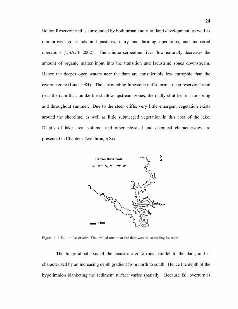
Belton Reservoir and is surrounded by both urban and rural land development, as well as
unimproved grasslands and pastures, dairy and farming operations, and industrial
operations (USACE 2002). The unique serpentine river flow naturally decreases the
amount of organic matter input into the transition and lacustrine zones downstream.
Hence the deeper open waters near the dam are considerably less eutrophic than the
riverine zone (Lind 1984). The surrounding limestone cliffs form a deep reservoir basin
near the dam that, unlike the shallow upstream zones, thermally stratifies in late spring
and throughout summer. Due to the steep cliffs, very little emergent vegetation exists
around the shoreline, as well as little submerged vegetation in this area of the lake.
Details of lake area, volume, and other physical and chemical characteristics are
presented in Chapters Two through Six.
Figure 1.1: Belton Reservoir. The circled area near the dam was the sampling location. The longitudinal axis of the lacustrine zone runs parallel to the dam, and is
characterized by an increasing depth gradient from north to south. Hence the depth of the
hypolimnion blanketing the sediment surface varies spatially. Because fall overturn is

25
often a gradual process, the shallower depths undergo mixing days or weeks before
greater depths, providing a temporal component to stratification and mixing events. To
capture both the spatial and temporal component of stratification and its effects on the
SWI, five sites along a linear transect along the longitudinal depth gradient were chosen.
These sites were not equally spaced, but instead chosen to represent the overall depth
gradient of the lacustrine zone.
The following chapters refer to these sites as Sites A – E, from shallowest to
deepest, respectively (Figure 1.2). Because the studies were conducted at different time
scales, the mean depth of these sites varied depending on various seasons with greater or
lesser rainfall and/or changing rates of water release from the dam. Site A, the most
shallow site is deeper than the mean depth of the reservoir (10.7 m); however mean depth
considers the depth of the extremely long and shallow riverine zone. In addition, several
deep holes occur in the lacustrine zone, some as deep as 37 m, however most of the
deepest sites near the dam are approximately 27 m, which corresponds to Site E.
Figure 1.2: Close up map of Belton Reservoir sampling sites. Sites increase in depth from A through E.

26
Sediments from these sites were always similar in consistency, composed of fine
clay. Most were very compact, allowing for little sediment porewater penetration.
Another unique attribute was the lack of benthic macroinvertebrates (e.g. crustaceans,
worms) within all SWI samples, both aerobic and anaerobic. Also, much discussion has
arisen about the presence of perchlorate contamination within Belton Reservoir sediments
from upstream industrial inputs, which are no longer being produced and released into the
watershed. A 2002 study by the United States Army Corps of Engineers suggested
further investigations be conducted on the effects of perchlorate levels in Belton
Reservoir on toxicity to fishes, plants, and microbiota (USACE 2002), however as of
2006 no other studies have been performed on perchlorate levels of Belton Reservoir.
27
CHAPTER TWO
Increased Sediment-Water Interface Bacterial [3H]-L-Serine Uptake and Biomass
Production in a Eutrophic Reservoir during Summer Stratification
Introduction
Sediment-water interfaces (SWIs) of lakes and reservoirs offer sites of intense
organic matter degradation and deposition (Butorin 1989; Dean 1999; Heinen and
McManus 2004). SWI carbon cycling occurs via microbial oxidation of dissolved and
particulate organic carbon (DOC and POC) and incorporation of DOC into bacterial
biomass via secondary production (Schallenberg and Kalff 1993; King 2002). This
linking of DOC to heterotrophic bacterial production defines the microbial loop (Wetzel
2001). While the microbial loop is traditionally defined in terms of planktonic microbial
dynamics, sediment bacteria may play an important role in the microbial loop and
ecosystem eutrophication processes (O’Loughlin and Chin 2004).
In thermally stratified reservoirs, bacterial metabolism often depletes dissolved
oxygen below the metalimnion resulting in an anoxic hypolimnion and SWI.
Hypolimnetic and SWI bacterial consortia respond to this oxygen depletion through the
use of alternate and less energetically favorable electron acceptors (Sweerts et al. 1991;
Liikanen and Martikainen 2003). Because many SWI bacteria are not facultative in their
respiratory functions, the bacterial community must shift their composition and
metabolism in response to anoxia (Kelly et al. 1988; Rosselló-Mora et al. 1999).
However, shifts in SWI bacterial activities and biomass production throughout seasonal
transitions of anoxia and mixing in reservoirs are poorly understood.
28
Bacterial activity and production in aquatic and sediment environments are
commonly measured via uptake of radiolabeled substrates such as 3H or 14C labeled L-
leucine or thymidine as a measure of bacterial protein synthesis or DNA synthesis,
respectively (Bell 1993; Kirchman 1993; Ducklow 2000; Chin-Leo 2002). These
substrates are well accepted for bacterial production studies; however advantages of
using these isotopes are often based on theoretical rather than empirical data. Ideally, the
radiolabeled substrate used for bacterial uptake should be metabolized under all
environmental conditions (e.g. dissolved oxygen, temperature, redox potential) imposed
in the study. For example, exogenous thymidine cannot be taken up by a variety of
sulfate reducing bacteria, chemolithotrophs, and methanogens—bacteria that are
commonly found in anoxic environments, such as SWIs (Johnstone and Jones 1989;
Gilmour et al. 1990).
[3H]-L-serine (Ser) was utilized to assess seasonal changes in SWI bacterial
activity and production. While Ser is not commonly used to measure bacterial uptake
rates and activity, this amino acid was chosen based on preliminary studies involving
various unlabeled amino acid, carbohydrate, and carboxylic acid uptakes rates by SWI
bacteria. Of these substrates, Ser exhibited high uptake by SWI bacteria under various
physicochemical conditions as well as having a high direct correlation with bacterial
abundance. These data provided empirical evidence that Ser could be used reliably as a
radiolabeled substrate to measure SWI bacterial uptake rates and estimate biomass
production without bias due to physical and chemical changes during stratification and
mixing.
29
Using Ser, this investigation sought to understand seasonal changes in bacterial
activity and production at the SWI of a seasonally stratified eutrophic reservoir and relate
seasonal SWI physicochemical variables to variations in SWI bacterial activity and
production. Providing a measure of seasonal SWI bacterial production is necessary if we
are to adequately understand microbial loop processes and food web dynamics in lake
and reservoir ecosystems.
Materials and Methods
Study Site and Sampling Protocol
Belton Reservoir, a deep, subtropical eutrophic reservoir located in central Texas,
served as the study site. Belton Reservoir is monomictic, undergoing thermal
stratification in late spring and maintaining an anoxic hypolimnion until overturn and
thermal mixing in mid-autumn (Christian et al. 2002; Christian and Lind 2006). The
reservoir basin has a maximum depth of 37 m, surface area of 49.8 km2, and a total
volume of 5.45 x 10⁸ m3. Secchi visibility ranges from 1.2 m to 2 m.
Five sample sites along a 1 km linear transect representative of the reservoir depth
gradient were sampled quarterly. Each consecutive site increased in depth, offering sites
that underwent thermal stratification in a sequential order. These differed in their
physicochemical variables on a spatial and temporal basis (Table 2.1), with the deepest
site (Site E, mean depth 25.9 m) becoming anoxic (dissolved oxygen < 0.2 mg l-1) and the
shallowest site (Site A, mean depth 13.4 m) becoming hypoxic (dissolved oxygen < 3 mg
l-1) during summer stratification. SWI temperature (°C), dissolved oxygen (mg l-1), pH,

30
specific conductivity (mS cm-1), and redox potential (mV) were measured at each site on
a seasonal basis using a YSI 600 QS Data Sonde.
Table 2.1: Physicochemical characteristics and bacterial abundance at the five SWI sampling sites (A-E) of increasing depth measured seasonally over one year. Variation in depth at each site through time is due to
fluctuating reservoir water levels.
Date Site Depth Temperature Dissolved pH Redox Specific Bacteria(m) (°C) Oxygen (mg l-1) (mV) Conductance x 106 ml-1
(mS cm-1)
14-Oct-04 A 13.8 24.6 7.4 7.1 431 0.80 1.0614-Oct-04 B 16.8 24.6 7.2 6.9 405 0.81 1.4614-Oct-04 C 20.2 24.6 5.3 6.9 411 0.80 2.2514-Oct-04 D 22.2 24.6 6.8 6.9 415 0.80 2.1514-Oct-04 E 26.2 24.5 6.6 6.5 341 0.81 3.11
3-Feb-05 A 14.5 10.9 9.5 7.2 398 0.91 1.513-Feb-05 B 16.4 10.9 9.4 7.1 405 0.91 1.293-Feb-05 C 20.0 10.9 9.7 7.2 393 0.91 1.413-Feb-05 D 23.4 11.2 9.1 7.1 454 0.92 1.273-Feb-05 E 26.2 11.1 9.4 7.4 459 0.90 1.5
1-Jun-05 A 13.3 20.2 2.9 7.0 380 1.11 2.621-Jun-05 B 16.4 18.5 2.8 7.0 398 1.12 1.621-Jun-05 C 20.0 16.7 2.1 6.9 393 1.12 1.511-Jun-05 D 22.8 16.5 1.7 7.0 391 1.11 1.111-Jun-05 E 26.1 16.4 1.1 7.0 420 1.11 2.26
21-Oct-05 A 13.0 24.0 4.6 7.0 243 0.93 1.2521-Oct-05 B 15.9 23.5 0.3 6.8 309 0.93 1.1821-Oct-05 C 19.3 22.9 0.2 6.6 228 0.95 1.0521-Oct-05 D 22.5 20.8 0.3 6.7 175 1.12 2.0621-Oct-05 E 25.0 19.9 0.2 6.6 159 1.16 1.06
Samples were collected at times corresponding to the onset of autumnal overturn
(Oct 2004), winter mixis (Feb 2005), onset of summer stratification (Jun 2005), and late-
season stratification (Oct 2005), respectively. Samples were retrieved by a 3.2 l
horizontal Alpha water sampler, positioned at the sediment surface. This allowed
sampling of the benthic boundary layer, defined as the water layer near the sediment
surface that contains a steep gradient in physicochemical variables due to the sediment
31
itself (Boudreau and Jørgensen 2001). The sampler was rinsed with demineralized water
between sample hauls to minimize sample cross-contamination. Duplicate samples from
each site, consisting of water and sediment particles, were pooled together in 300 ml dark
BOD bottles and immediately capped to prevent traces of oxygen contamination. Bottles
were placed in Styrofoam containers containing water collected at sampling depth to
maintain in situ temperature. Samples were returned to the laboratory for processing
within 3 hours of collection.
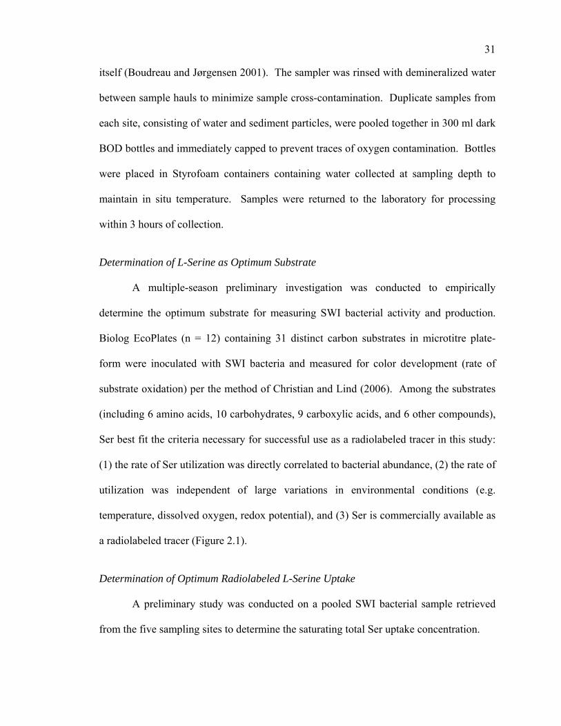
Determination of L-Serine as Optimum Substrate A multiple-season preliminary investigation was conducted to empirically
determine the optimum substrate for measuring SWI bacterial activity and production.
Biolog EcoPlates (n = 12) containing 31 distinct carbon substrates in microtitre plate-
form were inoculated with SWI bacteria and measured for color development (rate of
substrate oxidation) per the method of Christian and Lind (2006). Among the substrates
(including 6 amino acids, 10 carbohydrates, 9 carboxylic acids, and 6 other compounds),
Ser best fit the criteria necessary for successful use as a radiolabeled tracer in this study:
(1) the rate of Ser utilization was directly correlated to bacterial abundance, (2) the rate of
utilization was independent of large variations in environmental conditions (e.g.
temperature, dissolved oxygen, redox potential), and (3) Ser is commercially available as
a radiolabeled tracer (Figure 2.1).
Determination of Optimum Radiolabeled L-Serine Uptake
A preliminary study was conducted on a pooled SWI bacterial sample retrieved
from the five sampling sites to determine the saturating total Ser uptake concentration.
32
-0.6 0.6
-0.8
0.8
L-Serine
Temperature (C)
Dissolved Oxygen (mg l-1)
pH
Redox (mV)
Sp. Cond. (mS cm-1)
Bacteria ml-1
RDA Axis I
RDA
Axis
II
Figure 2.1: Redundancy Analysis (RDA) biplot with RDA axes I and II indicating loadings for environmental variables and SWI bacterial L-serine uptake from Biolog EcoPlate assays. Data was from a preliminary multi-seasonal study conducted on the Lake Belton SWI. L-serine was used by SWI bacteria independently of dissolved oxygen and pH, almost independently of temperature and dissolved oxygen, and positively correlated to bacterial abundance as indicated by perpendicular arrows (completely independent) or parallel arrows (positively correlated).
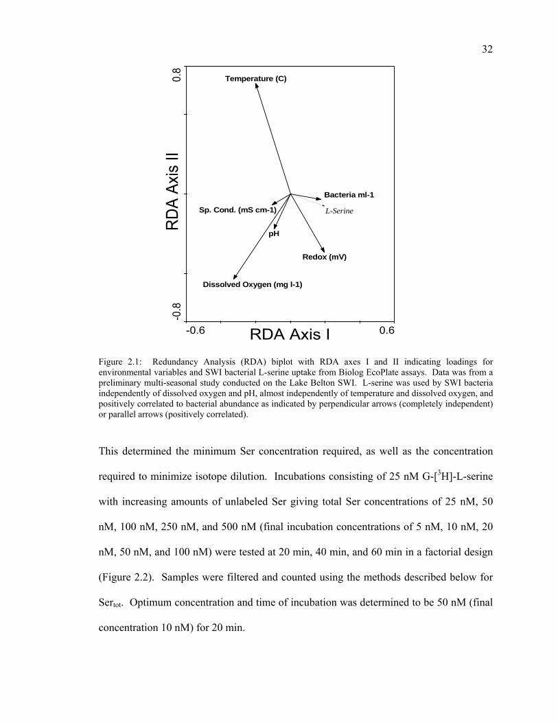
This determined the minimum Ser concentration required, as well as the concentration
required to minimize isotope dilution. Incubations consisting of 25 nM G-[3H]-L-serine
with increasing amounts of unlabeled Ser giving total Ser concentrations of 25 nM, 50
nM, 100 nM, 250 nM, and 500 nM (final incubation concentrations of 5 nM, 10 nM, 20
nM, 50 nM, and 100 nM) were tested at 20 min, 40 min, and 60 min in a factorial design
(Figure 2.2). Samples were filtered and counted using the methods described below for
Sertot. Optimum concentration and time of incubation was determined to be 50 nM (final
concentration 10 nM) for 20 min.
33
0
50
100
150
200
20 40 60
Incubation Time (min)
Tota
l Upt
ake
(Ser
tot)
(nm
ol l-1
h-1
)
25 nM50 nM100 nM250 nM500 nM
Figure 2.2: Sertot at various incubation times and concentrations from a pooled aerobic SWI bacterial sample taken from five SWI sites. 25 nM G-[3H]-L-serine was used with increasing concentrations of unlabeled L-serine for concentrations of 25 nM, 50 nM, 100 nM, 250 nM, and 500 nM. L-Serine Incubations
Three ml sterile plastic syringes fitted with 16-guage needles were prepared with
0.5 mL of 50 nM L-serine solution, specific activity 15.5 Ci mol-1. For anaerobic
incubations, the syringes and L-serine solution were first purged with nitrogen gas to
remove traces of oxygen. Two ml of sample was drawn into the syringe for a final Ser
concentration of 10 nM. Incubations were conducted by placing the inoculated syringes
in plastic bags, purging the bags with nitrogen if samples were anaerobic, and immersing
the bags in water adjusted to collection depth temperature. After 20 min, incubations
were stopped by adding 0.5 ml of formalin (final concentration 2 percent) to the syringe.
Zero-time killed controls were performed by adding formalin to syringes immediately
after sample inoculation. All sample and control incubations were performed in
34
quadruplicate which resulted in a coefficient of variation among sample activities of less
than 10 percent. Samples were held in the syringes at 4°C until radioassays were
performed.
Total L-Serine Uptake
To measure total bacterial uptake of Ser (Sertot), one-half (1.5 ml) of each
preserved sample was filtered through a 0.45 µm cellulose nitrate filter followed by
rinsing the filter three times with bacteria-free (0.2 µm-filtered) water. Each filter was
dried overnight and added to 1 ml of ethyl acetate in a 20 ml plastic scintillation vial.
After allowing the filters to dissolve overnight, 9 ml of scintillation cocktail (Ultima Gold
LLT) was added to the scintillation vial and vortexed. Vials were radioassayed on a
Beckman LS 6500 liquid scintillation counter at a counting precision of 5 percent error.
Samples were corrected for quench and counts per minute (CPMs) were converted to
disintegrations per minute (DPMs) using an external quench curve composed from a
series of commercially purchased quenched tritium standards.
L-Serine Uptake in Protein
To account for Ser exclusively in the protein fraction (Serpro), the other half of the
preserved sample (1.5 ml) was added to a 2 ml microcentrifuge tube containing a 0.5 ml
solution of 20% (w/v) NaCl and (v/v) trichloroacetic acid (TCA) (final concentration of
TCA/NaCl 5%). The microcentrifuge tubes were heated at 80°C for 30 min to precipitate
proteins, followed by centrifugation at 12,000 x g for 10 min. The supernatant was
discarded, and 1.5 ml of 80 % ethanol added. The tubes were centrifuged again at 12,000
x g for 10 min and the supernatant discarded. This ethanol wash step was performed

35
three times. One and a half ml of scintillation cocktail was added to the centrifuge tubes
and vortexed. The centrifuge tubes were placed in 20 ml scintillation vials and
radioassayed as above.
Bacterial Enumeration
Aliquots of each retrieved sample were preserved with formalin (2% final
concentration) for bacterial enumeration. Bacteria were stained with DAPI fluorochrome
at a final concentration of 5 µg ml-1. After staining, the samples were filtered through 0.2
µm blackened Nuclepore filters, placed on glass slides with a coverslip, and viewed
under UV light (330 nm – 380 nm) at 1500 x magnification. Ten fields, corresponding to
at least 300 bacteria were counted. Total bacteria per ml were calculated from the total
area of the filter counted and amount of sample filtered (Porter and Feig 1980).
Enumeration of bacteria attached to sediment particles were multiplied by 2 to correct for
masking of bacteria by the sediment particle.
Statistical Analyses
All summary statistics were analyzed using Microsoft Excel 2003. Other
statistical analyses were performed using JMP 5.0 (SAS Institute) or CANOCO 4.5
(Microcomputer Power) (ter Braak and Šmilauer 2002; Lepš and Šmilauer 2003).
Graphical analyses were performed using Microsoft Excel or CanoDraw 3.0 for
Windows, packaged with the CANOCO program.
Results
Sertot and bacterial abundance at each SWI site for all sampling seasons is shown
in Figure 2.3. A two-way repeated measures analysis of covariance (ANCOVA)
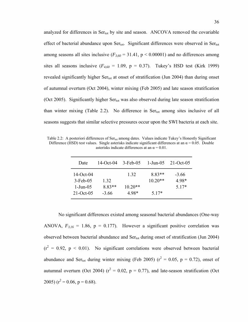
36
analyzed for differences in Sertot by site and season. ANCOVA removed the covariable
effect of bacterial abundance upon Sertot. Significant differences were observed in Sertot
among seasons all sites inclusive (F3,60 = 31.41, p < 0.00001) and no differences among
sites all seasons inclusive (F4,60 = 1.09, p = 0.37). Tukey’s HSD test (Kirk 1999)
revealed significantly higher Sertot at onset of stratification (Jun 2004) than during onset
of autumnal overturn (Oct 2004), winter mixing (Feb 2005) and late season stratification
(Oct 2005). Significantly higher Sertot was also observed during late season stratification
than winter mixing (Table 2.2). No difference in Sertot among sites inclusive of all
seasons suggests that similar selective pressures occur upon the SWI bacteria at each site.
Table 2.2: A posteriori differences of Sertot among dates. Values indicate Tukey’s Honestly Significant Difference (HSD) test values. Single asterisks indicate significant differences at an α = 0.05. Double
asterisks indicate differences at an α = 0.01.
Date 14-Oct-04 3-Feb-05 1-Jun-05 21-Oct-05
14-Oct-04 1.32 8.83** -3.663-Feb-05 1.32 10.20** 4.98*1-Jun-05 8.83** 10.20** 5.17*
21-Oct-05 -3.66 4.98* 5.17*
No significant differences existed among seasonal bacterial abundances (One-way
ANOVA, F3,16 = 1.86, p = 0.177). However a significant positive correlation was
observed between bacterial abundance and Sertot during onset of stratification (Jun 2004)
(r2 = 0.92, p < 0.01). No significant correlations were observed between bacterial
abundance and Sertot during winter mixing (Feb 2005) (r2 = 0.05, p = 0.72), onset of
autumnal overturn (Oct 2004) (r2 = 0.02, p = 0.77), and late-season stratification (Oct
2005) (r2 = 0.06, p = 0.68).
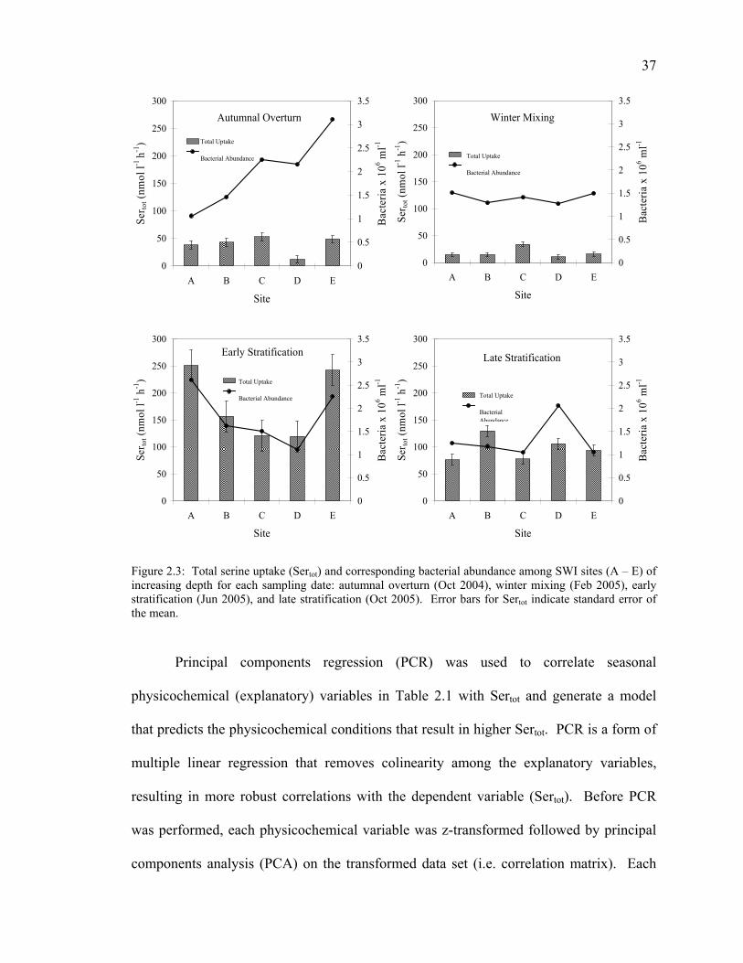
37
Autumnal Overturn
0
50
100
150
200
250
300
A B C D E
Site
Ser to
t (nm
ol l-1
h-1)
0
0.5
1
1.5
2
2.5
3
3.5
Bac
teria
x 1
06 ml-1nmol L-1 h-1
Bacteria x106 ml-1Total Uptake
Bacterial Abundance
Winter Mixing
0
50
100
150
200
250
300
A B C D E
Site
Ser to
t (nm
ol l-1
h-1
)
0
0.5
1
1.5
2
2.5
3
3.5
Bac
teria
x 1
06 ml-1
nmol L-1 h-1Bacteria x106 ml-1
Total Uptake
Bacterial Abundance
Early Stratification
0
50
100
150
200
250
300
A B C D E
Site
Ser to
t (nm
ol l-1
h-1
)
0
0.5
1
1.5
2
2.5
3
3.5
Bac
teria
x 1
06 ml-1nmol L-1 h-1
Bacteria x106 ml-1Total Uptake
Bacterial Abundance
Late Stratification
0
50
100
150
200
250
300
A B C D E
Site
Ser to
t (nm
ol l-1
h-1
)
0
0.5
1
1.5
2
2.5
3
3.5
Bac
teria
x 1
06 ml-1
nmol L-1 h-1Bacteria x106 ml-1
Total Uptake
Bacterial Abundance
Figure 2.3: Total serine uptake (Sertot) and corresponding bacterial abundance among SWI sites (A – E) of increasing depth for each sampling date: autumnal overturn (Oct 2004), winter mixing (Feb 2005), early stratification (Jun 2005), and late stratification (Oct 2005). Error bars for Sertot indicate standard error of the mean.
Principal components regression (PCR) was used to correlate seasonal
physicochemical (explanatory) variables in Table 2.1 with Sertot and generate a model
that predicts the physicochemical conditions that result in higher Sertot. PCR is a form of
multiple linear regression that removes colinearity among the explanatory variables,
resulting in more robust correlations with the dependent variable (Sertot). Before PCR
was performed, each physicochemical variable was z-transformed followed by principal
components analysis (PCA) on the transformed data set (i.e. correlation matrix). Each
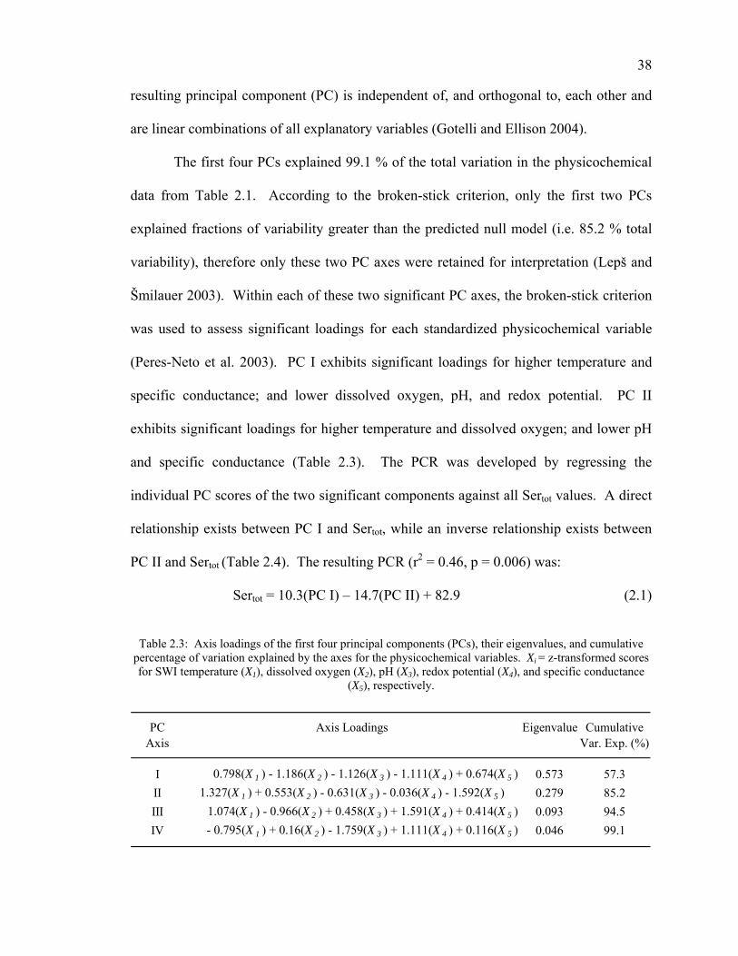
38
resulting principal component (PC) is independent of, and orthogonal to, each other and
are linear combinations of all explanatory variables (Gotelli and Ellison 2004).
The first four PCs explained 99.1 % of the total variation in the physicochemical
data from Table 2.1. According to the broken-stick criterion, only the first two PCs
explained fractions of variability greater than the predicted null model (i.e. 85.2 % total
variability), therefore only these two PC axes were retained for interpretation (Lepš and
Šmilauer 2003). Within each of these two significant PC axes, the broken-stick criterion
was used to assess significant loadings for each standardized physicochemical variable
(Peres-Neto et al. 2003). PC I exhibits significant loadings for higher temperature and
specific conductance; and lower dissolved oxygen, pH, and redox potential. PC II
exhibits significant loadings for higher temperature and dissolved oxygen; and lower pH
and specific conductance (Table 2.3). The PCR was developed by regressing the
individual PC scores of the two significant components against all Sertot values. A direct
relationship exists between PC I and Sertot, while an inverse relationship exists between
PC II and Sertot (Table 2.4). The resulting PCR (r2 = 0.46, p = 0.006) was:
Sertot = 10.3(PC I) – 14.7(PC II) + 82.9 (2.1)
Table 2.3: Axis loadings of the first four principal components (PCs), their eigenvalues, and cumulative
percentage of variation explained by the axes for the physicochemical variables. Xi = z-transformed scores for SWI temperature (X1), dissolved oxygen (X2), pH (X3), redox potential (X4), and specific conductance
(X5), respectively.
PC Axis Loadings Eigenvalue CumulativeAxis Var. Exp. (%)
I 0.798(X 1 ) - 1.186(X 2 ) - 1.126(X 3 ) - 1.111(X 4 ) + 0.674(X 5 ) 0.573 57.3II 1.327(X 1 ) + 0.553(X 2 ) - 0.631(X 3 ) - 0.036(X 4 ) - 1.592(X 5 ) 0.279 85.2III 1.074(X 1 ) - 0.966(X 2 ) + 0.458(X 3 ) + 1.591(X 4 ) + 0.414(X 5 ) 0.093 94.5IV - 0.795(X 1 ) + 0.16(X 2 ) - 1.759(X 3 ) + 1.111(X 4 ) + 0.116(X 5 ) 0.046 99.1

39
Table 2.4: The coefficients of the principal component regression (PCR) model derived from the significant principal components of the physicochemical data in table 3. The standard error, Student’s t-
ratio, and p-value for each coefficient are shown.
Variable Coefficient Std Error │t Ratio │ p-value
Intercept 82.9 12.4 6.7 < 0.0001PCA I 10.3 3.4 3.00 0.008PCA II -14.7 5.6 2.56 0.02
In addition to Sertot, incorporation of Ser into bacterial protein (Serpro) was also
measured. A significant positive linear correlation exists between Sertot and Serpro (r2 =
0.6, p < 0.0001, n = 20). The ratio of Sertot to Serpro did not change significantly among
seasons (F3,16 = 0.78, p = 0.53). The linear model associated with the correlation, when
forced through the origin, indicated that Serpro was approximately 40 percent of Sertot
(Figure 2.4).
y = 0.396xr2 = 0.6
0
25
50
75
100
125
150
0 50 100 150 200 250
Total Uptake (Sertot) (nmol l-1 h-1)
Prot
ein
Upt
ake
(Ser
pro)
(nm
ol l-1
h-1
)
Figure 2.4: Correlation biplot of total serine uptake (Sertot) vs. serine uptake in protein (Serpro), all sampling seasons inclusive. Linear regression equation is forced through the origin.
40
To convert Ser uptake into bacterial biomass production (expressed as grams of
carbon) a theoretical conversion factor of 5.5 mole-percentage of Ser in bacterial protein
was used (Reeck 1973; Reeck and Fisher 1973). Therefore bacterial biomass production
(BBP):
BBP (gC l-1 h-1) = Serpro x (molecular weight of L-Serine ÷ mol % Ser in protein)
x cell carbon per protein x isotope dilution (2.2) Where Serpro is in units of nmol l-1 h-1, molecular weight of L-serine = 105.1, mole
percentage L-serine in protein = 0.055 (5.5%), cell carbon per protein = 0.86, and isotope
dilution is 1, assuming that added Ser is in excess of intracellular Ser pools.
Equation 1 is modified from the equation of Kirchman (1993, 2001) which
utilizes L-leucine uptake. Mole percentage of Ser in bacterial protein was derived from
the source Kirchman (1985) used to derive the percentage of L-leucine in protein (Reeck
1973). The cell carbon per protein conversion is based on Simon and Azam (1989).
Because cell abundance was measured in addition to Sertot and Serpro, total growth
rate (µ) and generation time (h) was calculated using the theoretical conversion factor of
20 fg of carbon per cell (Lee and Fuhrman 1987; Ducklow 2000) where:
Growth Rate (µ) = BBP x (cells-1 x 20 fgC cell-1)-1 (2.3)
and
Generation Time (h) = 0.693µ-1 (2.4) Generation time is an estimate of the doubling time, or time required to generate
the entire bacterial population. This equation is inclusive to the entire bacterial consortia,
therefore is a ‘global’ doubling time which includes non-growing (dormant) populations
and populations that are fast and slow growing.
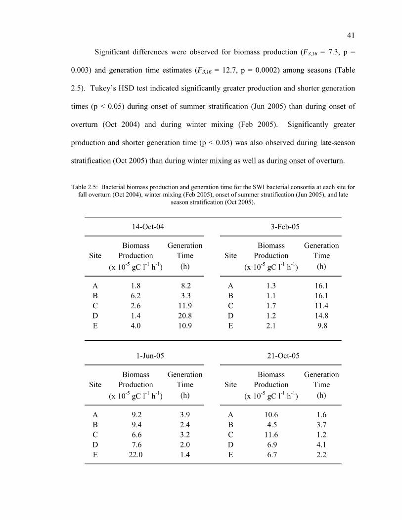
41
Significant differences were observed for biomass production (F3,16 = 7.3, p =
0.003) and generation time estimates (F3,16 = 12.7, p = 0.0002) among seasons (Table
2.5). Tukey’s HSD test indicated significantly greater production and shorter generation
times (p < 0.05) during onset of summer stratification (Jun 2005) than during onset of
overturn (Oct 2004) and during winter mixing (Feb 2005). Significantly greater
production and shorter generation time (p < 0.05) was also observed during late-season
stratification (Oct 2005) than during winter mixing as well as during onset of overturn.
Table 2.5: Bacterial biomass production and generation time for the SWI bacterial consortia at each site for
fall overturn (Oct 2004), winter mixing (Feb 2005), onset of summer stratification (Jun 2005), and late season stratification (Oct 2005).
14-Oct-04 3-Feb-05
Biomass Generation Biomass GenerationSite Production Time Site Production Time
(x 10-5 gC l-1 h-1) (h) (x 10-5 gC l-1 h-1) (h)
A 1.8 8.2 A 1.3 16.1B 6.2 3.3 B 1.1 16.1C 2.6 11.9 C 1.7 11.4D 1.4 20.8 D 1.2 14.8E 4.0 10.9 E 2.1 9.8
1-Jun-05 21-Oct-05
Biomass Generation Biomass GenerationSite Production Time Site Production Time
(x 10-5 gC l-1 h-1) (h) (x 10-5 gC l-1 h-1) (h)
A 9.2 3.9 A 10.6 1.6B 9.4 2.4 B 4.5 3.7C 6.6 3.2 C 11.6 1.2D 7.6 2.0 D 6.9 4.1E 22.0 1.4 E 6.7 2.2
42
Discussion
While the SWI zone is often arbitrarily defined (Novitsky 1983), it is commonly
recognized as a transition zone from fluid to solid matrix accompanied by a change in
redox potential (Danovaro et al. 1998). Further, Boudreau and Jørgensen defined this
zone as a ‘benthic boundary layer’ recognized as the location of chemical and energy
exchange between the water column and sediment bed marked by high biological activity
(2001). Changes in SWI redox potential are bacterially mediated by consumption and
production of organic matter while utilizing a variety of electron acceptors. Because
these organic matter cycles and changes in redox potential affect the quantity and quality
of nutrients, the trophic status, and overall water quality of the lake ecosystem, rates of
SWI bacterial activity and production are important in understanding microbial loop
processes.
Tritium labeled L-serine (Ser) uptake was measured for SWI bacterial consortia
using measures of Sertot and Serpro. Because few studies have used radiolabeled Ser (e.g.
Murrell et al. 1999), it was unknown what percentage of Ser was incorporated into
cellular protein, and what percentage was converted into other compounds. Our data
indicate that for short term uptake (i.e. 20 min) Serpro is approximately 40 % of Sertot.
Several reasons may account for the fate of introduced Ser not incorporated into protein.
First, methanotrophic and methylotrophic bacteria, commonly found at oxic/anoxic zones
such as the SWI, utilize Ser via a serine pathway to assimilate single-carbon compounds
into cell material via formation of an acetyl-CoA intermediate (Madigan et al. 1997).
Second, Ser may be incorporated into the bacterial cell wall as an interbridge component
in the peptidoglycan layer (White 1999). Third, flagella-containing bacteria display a cell
43
surface receptor (Tsr) that binds Ser, which serves as a chemoattractant to allow
functioning of the flagellar motor (Grebe and Stock 1998).
Because Ser may be incorporated into a variety of bacterial structures and
pathways, Sertot was chosen to compare differences in seasonal SWI bacterial uptake
rather than Serpro. When removing the covariable effect of bacterial abundance, highest
Sertot was observed at the onset of summer stratification (Jun 2005) (119 nmol l-1 h-1 –
251 nmol l-1 h-1) followed by late season stratification (Oct 2005) (76 nmol l-1 h-1 – 129
nmol l-1 h-1). Lowest Sertot was observed during winter mixis (Feb 2005) (14 nmol l-1 h-1
– 33 nmol l-1 h-1) and onset of autumnal overturn (Oct 2004) (11 nmol l-1 h-1 – 52 nmol l-1
h-1) (Figure 2.3(A) – 2.3(D)).
Bacterial abundance did not change significantly among seasons; however
bacterial abundance was coupled with high Sertot during the onset of stratification (Jun
2005) (Figure 2.3C). With the exception of Site D, this relationship also held for late-
season stratification (Oct 2005) (Figure 2.3D). The relationship did not exist during
overturn (Oct 2004) and winter mixis (Feb 2005) (Figure 2.3A and 2.3B). This coupling
indicates that during onset and late-season stratification, individual bacteria have a higher
specific Sertot than individual bacteria during onset of overturn and winter mixis. Higher
specific cell uptake rates during summer months, as well as evidence that 60 percent of
Ser is incorporated into protein suggest SWI bacteria during summer stratification
increase in biomass more so than bacteria during overturn and mixing.
Physicochemical variables related to seasonal stratification and mixing were
highly correlated (e.g. temperature and dissolved oxygen). Principal components (PCs)
were derived to statistically account for these correlations and relate the physicochemical
44
data to Sertot (Table 2.3). When the significant principal components were incorporated
into a regression (PCR), the resulting model predicted higher Sertot under SWI conditions
of higher temperature, lower dissolved oxygen, lower pH, lower redox and higher
specific conductance, consistent with late-season stratification. The model also predicted
higher Sertot under SWI conditions of lower temperature, lower dissolved oxygen, higher
pH, and higher specific conductance, consistent with the onset of stratification (i.e. late
spring, early summer) (Table 4).
Solely as a function of temperature, greater SWI bacterial Sertot would be
expected under higher temperatures due to increased function of metabolic enzymes (i.e.
the Q10 principle) (Atlas and Bartha 1998). Indeed, lowest Sertot was observed under
coldest conditions (Figure 2.3B), however highest activity was observed under
temperatures that were neither highest nor lowest during the course of this study. In most
cases, under high dissolved oxygen, Sertot was lower than during periods of oxygen
depletion. Possible reasons for this trend could be due to multiple electron acceptors
available to bacteria under cold, anoxic conditions (Kelly et al. 1988). During onset of
and during prolonged anoxia, redox potential decreases, resulting in a greater variety of
electron acceptors available to bacterial consortia not present under oxic conditions.
While facultative anaerobes would be active under oxic and anoxic conditions and a
variety of redox potentials, the remaining activity during anoxia would be due to strict
anaerobes. This suggests that strict anaerobes collectively may exhibit higher activity
than strict aerobes. This also supports evidence from an earlier study on Belton
Reservoir that demonstrated greater individual bacterial volumes and biomass in anoxic
45
hypolimnia (near the SWI) relative to the upper mixing and aerobic water column
(Christian et al. 2002).
Other physical factors may also account for seasonal differences in SWI bacterial
activity. During summer stratification, water movement at the SWI is negligible, with
fluxes between sediment and water occurring primarily through bioturbation, sinking of
organic matter from decaying and degraded phytoplankton, and reduced nutrients
entering the water column (Gantzer and Stefan 2003). Hence long-term stable bacterial
populations may form at the SWI without being flushed out or removed. In contrast,
during periods of overturn due to cooling and physical mixing, increased SWI water
movement and increased flux of sediment and nutrients may flush the bacteria out of the
SWI, resulting in frequent changes in SWI bacterial community composition and unstable
community structure. This contradicts other studies that have shown that faster water
movement during mixing brings in more bacterial substrates resulting in faster bacterial
substrate utilization (Boudreau and Jørgensen 2001; Gantzer and Stefan 2003).
Because Ser has not been commonly used as a measure of bacterial activity,
conversion factors for bacterial production are not well established. We have used the
value of 5.5 percent of total bacterial protein composed of L-serine. This value was
established by Reeck (1973) and Reeck and Fisher (1973) and is based on the amino acid
composition of 69 different purified bacterial proteins. Kirchman (1985) derived the
percent of L-leucine in protein based on this same source, which remains well accepted.
This conversion is theoretical however, and the true percentage of L-serine in protein
may differ for natural bacterial assemblages. Recently a conversion factor of 4.2 percent
L-serine in bacterial protein was derived from an analysis of freshwater sediment bacteria

46
(Buesing and Marxsen 2005). However, given the range of our measured uptake rates,
our values of bacterial production are comparable to that of L-leucine in a variety of
aquatic and sediment environments (Servais 1995; Tuominen 1995; Buesing and
Marxsen 2005).
Lastly, we estimated generation times of the SWI bacteria based on the equation
of Ducklow (2000) and estimates of cellular carbon (Lee and Fuhrman 1987). While
much debate has ensued about the amount of carbon per bacterium, 20 fg cell-1
established by Lee and Fuhrman is widely accepted. Shorter generation times were
observed during stratification and before autumnal overturn, implying higher rates of
reproduction, consistent with balanced growth. While there may be tremendous
variability in reproduction rates of individual populations, the values calculated represent
a total community average. Higher rates of reproduction are consistent with the onset of
and late-season stratification. During this time, calm SWI physical conditions prevail,
therefore bacteria can devote more energy into reproduction, rather than survival.
Conclusions
Our study has revealed that summer stratification and related physicochemical
dynamics drives SWI bacterial activity and biomass production at greater rates than
thermal mixing processes. Results show that SWI bacterial uptake rates of L-serine -
used as a surrogate of bacterial activity and biomass production - are greater during the
onset of summer stratification and during late season stratification. These rates are
independent of bacterial abundance, but during stratification bacterial abundance is
coupled with high Sertot, suggesting higher per-cell activity, consistent with higher rates
of cell reproduction. Several physicochemical dynamics that change during stratification
47
and overturn, including SWI temperature, dissolved oxygen and redox potential are
associated with and modeled to variations in Sertot. We conclude SWI bacterial
metabolism is more important in this reservoir’s carbon cycling during summer months
than during winter months, and therefore contributes an important role in nutrient
dynamics and eutrophication processes often attributed mostly to planktonic, and often
autotrophic, microorganisms.
Acknowledgments
Funding for this project was made possible by the Jack G. and Norma Jean
Folmar Research Grant and the Bob Gardner Memorial Grant through Baylor University.
We thank Christopher Filstrup and David Clubbs for valuable field assistance. We also
thank Dr. Diane Wycuff for assistance with radioisotope compliance and use.
48
CHAPTER THREE
Key Issues Concerning Biolog Use for Aerobic and Anaerobic Freshwater Bacterial Community-Level Physiological Profiling
Introduction Originally designed to rapidly identify cultured bacterial isolates, microbial
ecologists have tailored Biolog MicroPlates™ (e.g. GN and GP MicroPlates) to generate
bacterial community-level physiological profiles (CLPPs) from environmental matrices
such as soil, sewage sludge, and water. Applications and limitations of Biolog
MicroPlates for terrestrial bacterial community profiling are well documented (Smalla et
al. 1998; Balser et al. 2002; Classen et al. 2003; Insam and Goberna 2004). Aquatic
(freshwater and marine) bacterial communities have been profiled to a lesser extent (Choi
and Dobbs 1999; Grover and Chrzanowski 2000; Schultz and Ducklow 2000; Tam et al.
2003; Sala et al. 2005), consequently several methodological and analytical CLPP issues
involving aquatic bacterial assessment have not been adequately addressed.
Biolog MicroPlates contain 96 microtiter wells, each containing a distinct organic
carbon substrate and a redox-sensitive tetrazolium dye indicator. When plates are
inoculated with a bacterial community and incubated, purple formazan salt forms in each
well proportional to the extent of bacterial community substrate oxidation. Each well is
scored for substrate use or disuse or read for its optical density at 590 nm (OD590). The
resulting carbon substrate utilization pattern (CSUP) is used to develop the CLPP
(Garland and Mills 1991; Konopka et al. 1998).

49
In response to GN MicroPlate ecological use, Biolog developed the EcoPlate™,
containing, in triplicate, 31 organic carbon substrates and a control well with dye, but no
substrate (Table 3.1). EcoPlates provide intraplate replication, allowing for greater
statistical applications. EcoPlates contain 25 substrates common to GN plates, as well as
6 substrates unique to the EcoPlate. This suite of substrates was chosen to allow for
substrate utilization by a variety of metabolically diverse and slower growing bacteria
that are commonly found in environmental matrices (Preston-Mafham et al. 2002).
Table 3.1: List of all 31 carbon substrates in Biolog EcoPlates™, their corresponding classes, and plate
code numbers.
Substrate Plate Code Substrate Plate Code
Amino Acids (n = 6) Carboxylic Acids (n = 9) L-Arginine A4 γ-Hydroxybutyric Acid E3 L-Asparagine B4 α-Ketobutyric Acid G3 Glycyl-L-Glutamic Acid F4 D-Galacturonic Acid B3 L-Phenylalanine C4 D-Glucosaminic Acid F2 L-Serine D4 Itaconic Acid F3 L-Threonine E4 D-Malic Acid H3Carbohydrates (n = 10) Pyruvic Acid Methyl Ester B1 D-Cellobiose G1 2-Hydroxybenzoic Acid C3 i-Erythritol C2 4-Hydroxybenzoic Acid D3 D-Galactonic Acid γ-lactone A3 Amines (n = 2) N-Acetyl-D-Glucosamine E2 Phenylethylamine G4 Glucose-1-Phosphate G2 Putrescine H4 β-Methyl-D-Glucoside A2 Polymers (n = 4) D,L-α-Glycerol Phosphate H2 α-Cyclodextrin E1 α-D-Lactose H1 Glycogen F1 D-Mannitol D2 Tween 40 C1 D-Xylose B2 Tween 80 D1
While literature has addressed many Biolog MicroPlate limitations and
applications, this investigation addresses these issues as they apply directly to freshwater
50
heterotrophic bacterial community studies. The value of this is threefold. (1) Unlike
many environmental bacteria, aquatic bacteria differ in that their environmental matrix
allows direct inoculation; therefore microbial ecologists need a reference to specifically
address this significance. (2) Because heterotrophic bacteria dynamically impact organic
matter cycling in freshwater ecosystems (Van Mooy et al. 2001; Chin-Leo 2002), CSUPs
illustrate the potential complexity of organic matter cycling (Sinsabaugh and Foreman
2001; Tam et al. 2003). (3) CLPPs indicate bacterial community metabolic potential,
which provides insight into the overall functional diversity of heterotrophic bacterial
assemblages present in the ecosystem.
For general methodological and statistical issues involving a variety of Biolog
MicroPlates, the reader should refer to Konopka et al. (1998), Mills and Garland (2002),
and Preston-Mafham et al. (2002). Because of their design for ecological studies and
ease of statistical analysis, only EcoPlate usage is discussed. However, the information
presented is pertinent to other types of Biolog MicroPlates due to the similarity of their
design and applicability to aquatic bacterial communities.
Specifically the following topics are addressed: (1) The effect of aquatic bacterial
inoculum density on carbon substrate utilization rate, (2) The effects of incubation
temperature on carbon substrate utilization rate and pattern, (3) Well color development
due to non-bacterial entities in the inocula, (4) The extent of substrate selectivity, and (5)
Adaptation of EcoPlates for use in anaerobic aquatic bacterial community studies.
51
Materials and Methods Study Site Bacterioplankton samples were collected from Belton Reservoir, Bell County,
Texas, USA (31° 06’ N, 97° 28’ W), a subtropical, eutrophic monomictic reservoir
(Christian et al. 2002). Collection depths ranged from 13.5 m to 25.2 m. Water
temperature and dissolved oxygen concentration ranged from 10.9°C to 26.9°C and 0 mg
l-1 to 10.6 mg l-1, respectively, as measured with a YSI 600QS Sonde (YSI, Inc. Yellow
Springs, Ohio, USA).
General Methodology Samples were collected at various times before, during, and after autumnal
overturn to allow for differences in lake temperature and dissolved oxygen, as necessary
for analyses. Samples were taken from less than 0.1 m above the sediment-water
interface using a 3.2 l horizontal Alpha Water Sampler (Wildlife Supply Company,
Buffalo, New York, USA). Three hundred ml black BOD bottles were overflowed three
times with the sample and immediately capped to maintain in situ oxygen concentration.
The sampler was rinsed with bacteria-free (0.2 μm-filtered) water between sample hauls
to flush out remaining bacteria. The bottles were immersed in coolers containing water
collected at sampling depth so that in situ temperature was maintained. All samples were
returned to the laboratory within 4 to 6 hours of sample collection for immediate
processing.
EcoPlates were purchased directly from the manufacturer (Biolog Inc., Hayward,
California, USA) and stored at 4°C until use. All plates were inoculated with 150 µl of
sample water into each well using an 8-channel repeating pipettor fitted with 1 ml sterile
52
disposable pipettor tips. Plates were incubated (temperature depended on experiment)
and read at OD590 on a daily basis with a Biolog MicroStation 3 plate reader and
software. The data was transferred via the software to Microsoft Office Excel 2003.
JMP™ 5.0 (SAS Institute, Inc., Cary, North Carolina, USA), Microsoft Office Excel
2003, and SigmaPlot® 2000 (SPSS, Inc., Chicago, Illinois, USA) were used for statistical
and graphical analyses.
Mean OD590 for each substrate (n = 3) at each reading time (e.g. every 24 hours)
was corrected by subtracting the mean optical density of the control wells (n = 3) and
plotted against time. Because typical bacterial logistic growth was observed, a 3-
parameter sigmoidal curve was fitted to the data:
a y = ————— (3.1)
1 + e – (X-X0/b)
where x and y denote time of incubation and mean OD590 of the substrate at time x
respectively, a = the horizontal asymptote of maximum growth rate, b = the inverse of the
exponential growth rate, and X0 = the time at the midpoint of exponential growth
(Lindstrom et al. 1998). Likewise, the 3-parameter sigmoidal curve was fitted to the
average well color development (AWCD) at each reading time (y-axis) plotted against
time (x-axis):
AWCD(t) = ∑ (C(t) – R(t))/n (3.2)
where t = time of incubation, C(t) = mean color production (OD590) of a substrate at time t,
R(t) = mean color production in the control well at time t, and n = number of substrates
(i.e. 31 for EcoPlates) (Garland and Mills 1991; Choi and Dobbs 1999).

53
Inoculum Density Effects One ml aliquots from various samples collected before, during, and after
autumnal overturn were enumerated for total bacterial abundance. Samples were
preserved with an equal volume of 4% formalin and stored at 4°C until enumerated.
Each sample was stained with DAPI fluorochrome (1 µg ml-1, final concentration),
filtered onto a 0.2 µm polycarbonate black membrane filter, and viewed under UV
excitation (330 nm – 380 nm) with a Nikon Eclipse 6600 microscope at 1500 x total
magnification (Porter and Feig 1980). All bacteria in 20 fields, or 300 bacteria,
whichever came first, were counted. Initial bacterial abundance (inoculum density) was
regressed against the AWCD at each reading time for all samples (n = 50) to observe
correlation of inoculum density and extent of substrate utilization.
Incubation Temperature Experiment Samples were collected from all five sampling sites after autumnal mixis. Sample
collection temperatures ranged from 15.9°C to 16.5°C, and dissolved oxygen
concentration ranged from 4.5 mg l-1 to 8.4 mg l-1. Each sample was inoculated into two
EcoPlates, one incubated aerobically at near in situ temperature (15°C), the other
aerobically at room temperature (22°C). Substrate utilization rates and substrate
utilization pattern similarity were compared between the plates.
A simple matching coefficient was used to compare similarities for each substrate
response at each reading time between plates incubated at 15°C and 22°C. The use and
disuse of a carbon substrate was scored as a 1 or 0, respectively, where use was any
positive OD590 value when corrected for color development in the control well:
Substrate Similarity = S[15°C, 22°C] / (N15°C + N22°C – S[15°C, 22°C]) (3.3)

54
where S[15°C, 22°C] = total number of similar responses in corresponding wells at 15°C and
22°C (either 1 and 1 or 0 and 0), N15°C = number of substrates measured at 15°C (i.e. 31)
and N22°C = number of substrates measured at 22°C (i.e. 31).
Non-Bacterial Color Development Effects
Samples were collected from all five sampling sites after autumnal mixis, but
before cooling. Sample collection temperatures ranged from 24.5°C to 24.7°C, and
dissolved oxygen concentration from 6.5 mg l-1 to 7.4 mg l-1. Each sample was
partitioned, one half inoculated directly into an EcoPlate and the other half autoclaved for
15 min at 121°C and 103 kPa, cooled to room temperature, and inoculated into an
EcoPlate. Plates were incubated aerobically at room temperature (22°C). Substrate
utilization rates and AWCD at each reading point of raw samples were compared to
substrate utilization rates and AWCD at each reading point of autoclaved samples.
Substrate Selectivity Effects Equal volumes of the non-autoclaved portions of the water samples (n = 5) used
for the non-bacterial color development experiment were pooled and plated onto two
EcoPlates and incubated aerobically at room temperature (22°C). One ml of initial
inoculum was enumerated as above for the inoculum density experiment. In addition
counts were separated into total cocci and total bacilli. A 100 µl aliquot was removed
from all 32 different wells every 24 hours for four days and enumerated, with counts
separated into total cocci and total bacilli. Because each well was inoculated with 150 µl
of sample, new wells were sampled daily.

55
Anaerobic Community-Level Physiological Profiling
Numerous samples were retrieved from all sites during a prolonged period of
anoxia (summer stratification). Temperatures ranged from 14.9°C to 25°C. To process
an individual sample in the laboratory, the BOD bottle containing collection water was
uncapped and immediately purged with a stream of nitrogen gas via a 15 mm-diameter
aquarium tube fitted into the bottle. Sample was drawn gravimetrically from the bottle,
through 15 mm-diameter aquarium tubing, into a 25 ml sampling trough and overflowed
three times volume. The sample in the trough was continuously purged with nitrogen gas
while it was drawn into the 8-channel pipettor, in which the disposable pipet tips were
purged with nitrogen before and after fitting them to the pipettor. Samples were
immediately inoculated onto the plate under a blow down of nitrogen. The plates were
immediately covered with a non-slit silicone plate seal, with small volumes of water
displaced by the seal, preventing a headspace of air. The lid was placed on the plate and
double-sealed with tape.
Results
Inoculum Density There was a significant positive correlation between bacterial inoculum density
and AWCD after 24 hours of incubation (r2 = 0.73, p < 0.0001, n = 50) (Figure 3.1). This
correlation decreased with increasing incubation time (Table 3.2). Because low initial
cell inocula are associated with low rates of substrate utilization for short term
incubations, the initial density of cells plated impacts the duration of lag before
exponential growth is observed.
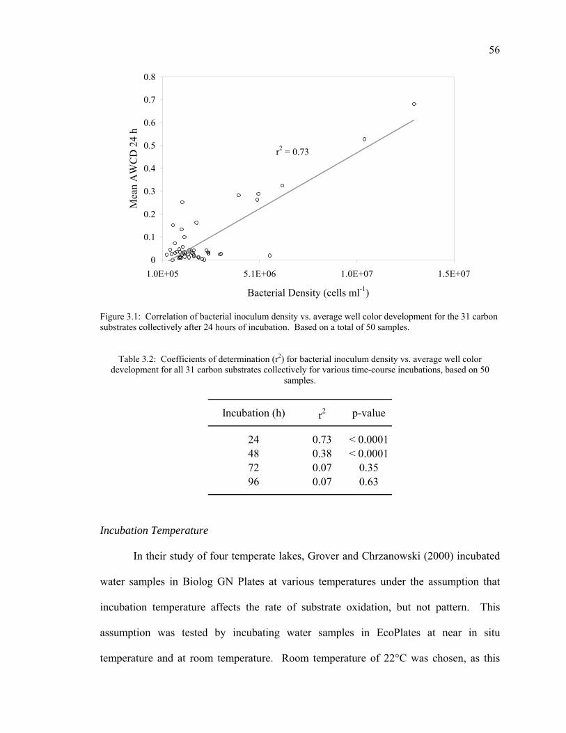
56
r2 = 0.73
0
0.1
0.2
0.3
0.4
0.5
0.6
0.7
0.8
1.0E+05 5.1E+06 1.0E+07 1.5E+07
Bacterial Density (cells ml-1)
Mea
n A
WC
D 2
4 h
Figure 3.1: Correlation of bacterial inoculum density vs. average well color development for the 31 carbon substrates collectively after 24 hours of incubation. Based on a total of 50 samples.
Table 3.2: Coefficients of determination (r2) for bacterial inoculum density vs. average well color
development for all 31 carbon substrates collectively for various time-course incubations, based on 50 samples.
Incubation (h) r2 p-value
24 0.73 < 0.000148 0.38 < 0.000172 0.07 0.3596 0.07 0.63
Incubation Temperature In their study of four temperate lakes, Grover and Chrzanowski (2000) incubated
water samples in Biolog GN Plates at various temperatures under the assumption that
incubation temperature affects the rate of substrate oxidation, but not pattern. This
assumption was tested by incubating water samples in EcoPlates at near in situ
temperature and at room temperature. Room temperature of 22°C was chosen, as this
57
was the temperature used by Grover and Chrzanowski for most of their incubations
(2000).
AWCD at each reading point and substrate utilization rates for the 15°C
incubations were less than for incubations at 22°C (Figure 3.2). 15°C plates were further
read at OD590 daily for a total of two weeks, each of which reached a μmax of
approximately 0.28 OD590 units (data not shown). It was therefore proposed that
differences in substrate utilization rate and AWCD were due to the elevated incubation
temperature causing a net increase in bacterial community metabolism. However, it was
uncertain if the increased temperature selected for bacterial species that do not metabolize
substrates at 15°C. Thus, substrate response similarity at multiple reading times between
both sets of plates was compared. Results of the matching coefficient (Table 3.3)
indicate that the highest similarity among plates incubated at 15°C and 22°C was
approximately 60% after 96 incubation hours. These results indicate that incubation
temperature has an effect CSUP, not just rate.
Table 3.3: Mean number of similar responses and mean similarity coefficient ± standard deviation for a series of paired plates (5 pair, one of the pair incubated at 15°C and the other at 22°C, each pair from a different water sample) at various times of incubation. Total possible number of similar responses (both
wells OD590 > 0, or both wells OD590 ≤ 0) per pair of plates is equal to the number of wells on a single plate (96).
Time of Mean Similar Mean SimilarityIncubation (h) Responses Coefficient ± S.D.
24 67.5 0.552 ± 0.14348 47.8 0.340 ± 0.11772 63.2 0.502 ± 0.15196 70.8 0.597 ± 0.165
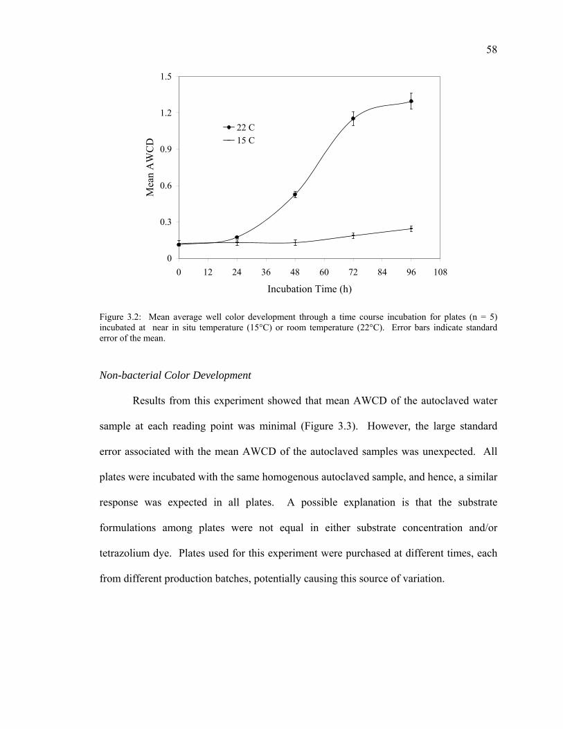
58
0
0.3
0.6
0.9
1.2
1.5
0 12 24 36 48 60 72 84 96 108
Incubation Time (h)
Mea
n A
WC
D
22 C15 C
Figure 3.2: Mean average well color development through a time course incubation for plates (n = 5) incubated at near in situ temperature (15°C) or room temperature (22°C). Error bars indicate standard error of the mean. Non-bacterial Color Development
Results from this experiment showed that mean AWCD of the autoclaved water
sample at each reading point was minimal (Figure 3.3). However, the large standard
error associated with the mean AWCD of the autoclaved samples was unexpected. All
plates were incubated with the same homogenous autoclaved sample, and hence, a similar
response was expected in all plates. A possible explanation is that the substrate
formulations among plates were not equal in either substrate concentration and/or
tetrazolium dye. Plates used for this experiment were purchased at different times, each
from different production batches, potentially causing this source of variation.
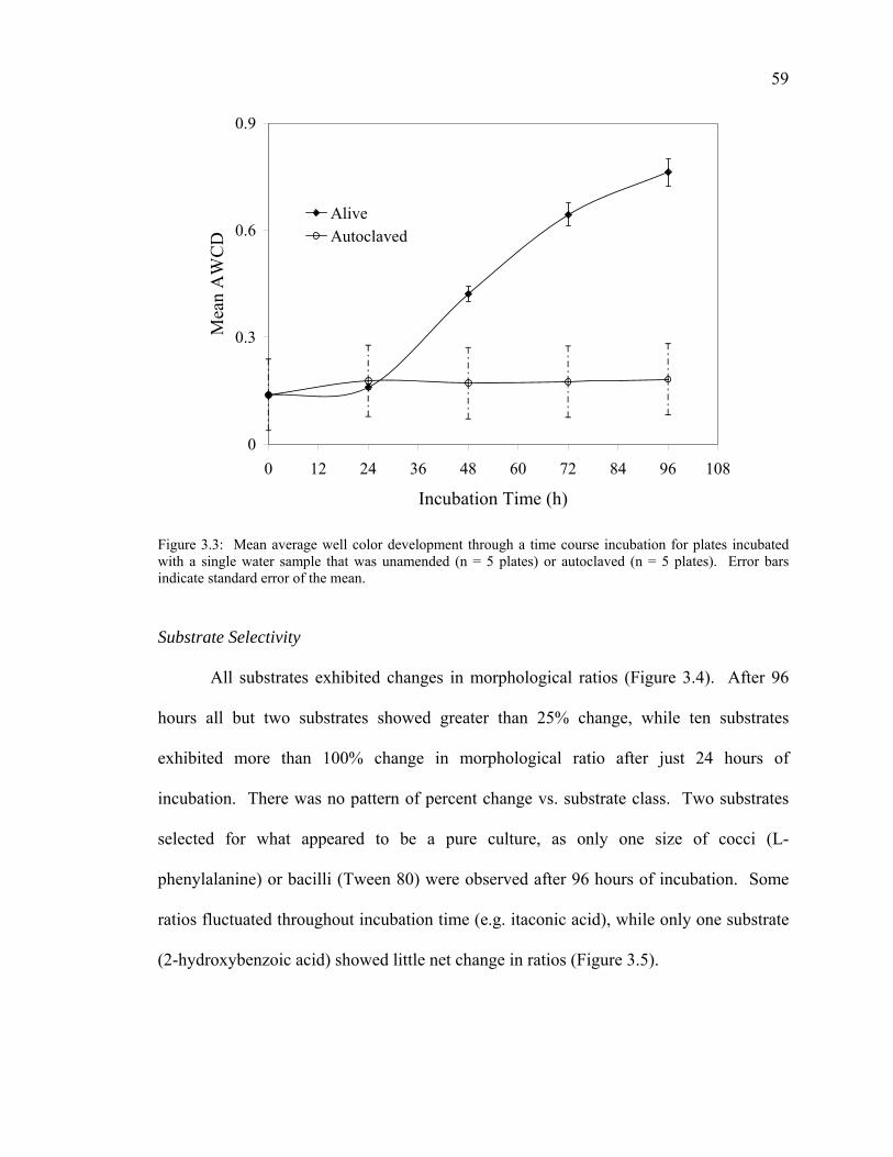
59
0
0.3
0.6
0.9
0 12 24 36 48 60 72 84 96 108
Incubation Time (h)
Mea
n A
WC
DAliveAutoclaved
Figure 3.3: Mean average well color development through a time course incubation for plates incubated with a single water sample that was unamended (n = 5 plates) or autoclaved (n = 5 plates). Error bars indicate standard error of the mean.
Substrate Selectivity
All substrates exhibited changes in morphological ratios (Figure 3.4). After 96
hours all but two substrates showed greater than 25% change, while ten substrates
exhibited more than 100% change in morphological ratio after just 24 hours of
incubation. There was no pattern of percent change vs. substrate class. Two substrates
selected for what appeared to be a pure culture, as only one size of cocci (L-
phenylalanine) or bacilli (Tween 80) were observed after 96 hours of incubation. Some
ratios fluctuated throughout incubation time (e.g. itaconic acid), while only one substrate
(2-hydroxybenzoic acid) showed little net change in ratios (Figure 3.5).
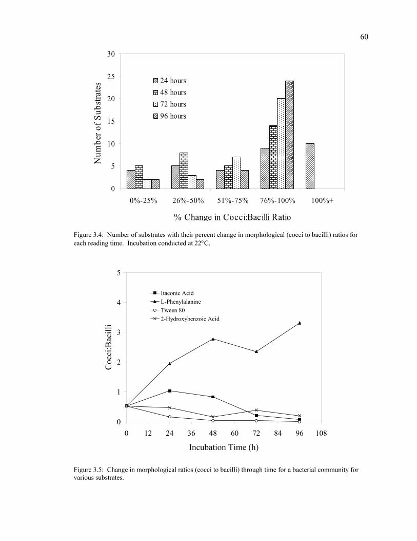
60
0
5
10
15
20
25
30
0%-25% 26%-50% 51%-75% 76%-100% 100%+
% Change in Cocci:Bacilli Ratio
Num
ber o
f Sub
strat
es
24 hours48 hours72 hours96 hours
Figure 3.4: Number of substrates with their percent change in morphological (cocci to bacilli) ratios for each reading time. Incubation conducted at 22°C.
0
1
2
3
4
5
0 12 24 36 48 60 72 84 96 108
Incubation Time (h)
Coc
ci:B
acill
i
Itaconic AcidL-PhenylalanineTween 802-Hydroxybenzoic Acid
Figure 3.5: Change in morphological ratios (cocci to bacilli) through time for a bacterial community for various substrates.
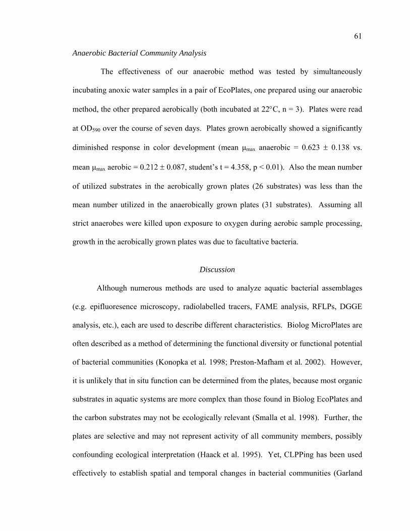
61
Anaerobic Bacterial Community Analysis
The effectiveness of our anaerobic method was tested by simultaneously
incubating anoxic water samples in a pair of EcoPlates, one prepared using our anaerobic
method, the other prepared aerobically (both incubated at 22°C, n = 3). Plates were read
at OD590 over the course of seven days. Plates grown aerobically showed a significantly
diminished response in color development (mean μmax anaerobic = 0.623 ± 0.138 vs.
mean μmax aerobic = 0.212 ± 0.087, student’s t = 4.358, p < 0.01). Also the mean number
of utilized substrates in the aerobically grown plates (26 substrates) was less than the
mean number utilized in the anaerobically grown plates (31 substrates). Assuming all
strict anaerobes were killed upon exposure to oxygen during aerobic sample processing,
growth in the aerobically grown plates was due to facultative bacteria.
Discussion
Although numerous methods are used to analyze aquatic bacterial assemblages
(e.g. epifluoresence microscopy, radiolabelled tracers, FAME analysis, RFLPs, DGGE
analysis, etc.), each are used to describe different characteristics. Biolog MicroPlates are
often described as a method of determining the functional diversity or functional potential
of bacterial communities (Konopka et al. 1998; Preston-Mafham et al. 2002). However,
it is unlikely that in situ function can be determined from the plates, because most organic
substrates in aquatic systems are more complex than those found in Biolog EcoPlates and
the carbon substrates may not be ecologically relevant (Smalla et al. 1998). Further, the
plates are selective and may not represent activity of all community members, possibly
confounding ecological interpretation (Haack et al. 1995). Yet, CLPPing has been used
effectively to establish spatial and temporal changes in bacterial communities (Garland
62
1997) as well as providing insight into functional ability of bacterial community members
(Preston-Mafham et al. 2002).
Unlike soil or sediment CLPPing, aquatic systems offer the advantage of being
able to inoculate the environmental matrix (water) directly into the wells without dilution
or major disruption of the community. Yet bacterial abundance in aquatic ecosystems is
variable on both spatial and temporal scales (Christian and Capone 2002), therefore
variable bacterial abundances inoculated directly from the environment without first
standardizing the inoculum density will affect rate of substrate utilization. This
investigation shows that for short term incubations, lower inocula densities results in a
longer lag phase before substrate is utilized. It could be argued that enumerating the
bacteria via DAPI or acridine orange staining followed by dilution to a known
concentration and using the diluted consortia for inoculation is a valid method, however
this may eliminate bacteria that show strong response to substrate utilization, but are
present in low numbers. It is also possible that dilution may alter ratios of individual
populations that strongly contribute to overall response, which will affect the rate.
This finding is also important from an analytical standpoint. For example, the
OD590 of a substrate at a single time point divided by the AWCD at that time point is
often used as the metric for determining CSUPs (Glimm et al. 1997; Insam and Goberna
2004). If the time point is unknowingly chosen before exponential growth has began for
all substrates, the resulting metric will underestimate the actual carbon substrate
utilization pattern. To alleviate this problem, the use of a kinetic instead of a single time-
point approach is suggested, in which the rate of exponential growth (equation 1) is used
as the metric to develop the CSUP. While using a kinetic approach is not novel, it allows
63
the investigator to preserve the relative abundance of the entire bacterial community,
providing a better estimate of community functional potential.
Because CLPPs are a measure of ‘functional potential’, then incubation
temperature should be reported with all results. This investigation has shown that
altering incubation temperature results not only in variation of color response in all wells,
but also response pattern. If various incubation temperatures are used for a spatial or
time course study, CSUP differences will be confounding, making it impossible to assess
spatial and temporal CSUP differences from differences due to the selectiveness of
varying incubation temperature. Therefore incubation temperature should be standardized
across all incubations if spatial and/or temporal community studies are to be undertaken.
This is not to imply that any certain incubation temperature is ‘optimum’, because the
temperature may not reflect in situ temperature. However if this temperature is applied
consistently, one may eliminate possibility of CSUP differences due to varying
temperatures.
When interpreting CSUPs, it has been assumed that all color development from
tetrazolium dye reduction is due to bacterial carbon substrate oxidation, however
previous to this investigation this remained untested. By plating an autoclaved water
sample, all living organisms were killed (e.g. bacteria, viruses, microeukaryotes), leaving
only complex organic and inorganic nutrients, waste products, metals, and toxins in the
water sample to react with the carbon substrates and produce insoluble formazan. By
plating autoclaved water samples and comparing the response to unamended water
samples, it was deduced from the high standard error associated with utilization rates of
the autoclaved samples that all plates for a single investigation should be from the same
64
production batch to minimize any differences in substrate and tetrazolium dye
concentration. Each well is said to contain 0.3 mg of carbon substrate (Mills and Garland
2002), but even small deviations from this amount may drastically affect substrate
utilization rate. Plates from the same batch are likely to contain more similar and
consistent formulations of substrates than plates produced in different batches.
If high rates of non-bacterial tetrazolium dye reduction are suspected, killed
controls should be run under the same conditions as sample plates and a correction factor
applied to the color development of each well. Furthermore, while the carbon substrates
are formulated in a concentration for bacterial use, it is uncertain if a portion of the total
substrate oxidation is due to heterotrophic eukaryotic microorganisms.
Many researchers assume that individual wells of Biolog MicroPlates are
analogous to selective culturing media, however the extent of individual substrate
selectivity has not been tested on aquatic microbial assemblages. If the carbon substrates
are not strongly selective, at any given time point, bacterial morphological ratios (i.e.
cocci to bacilli) would be similar to their ratios in the initial inoculum. Significant
changes in morphological ratios would indicate selectivity for certain populations. This
investigation empirically shows that Biolog is a selective culturing technique. The results
indicate that selectivity varies among substrates, but all substrates exhibit some degree of
selectivity. This selectivity may be due to several factors: (1) only organisms that can
grow under the constrained conditions imposed will contribute to color response in the
individual wells, (2) inoculum density, and/or (3) activity/dormancy of specific
populations. Further, the results support the suggestion that CLPPs are a measure of
functional potential, not in situ ecological potential, therefore any attempts to imply

65
ecological function should be approached with caution. Yet, previous studies suggested
that incubations of less than 24 h may closely represent in situ function (Mills and
Garland 2002). However, use of a preferred class of substrate by a bacterial community
(e.g. carbohydrates, amino acids) may indicate nutritional needs of the bacteria and
therefore provide insight into community metabolic status.
Many aquatic systems contain anaerobic habitats (e.g. anoxic hypolimnia of lakes,
anaerobic wetlands), but obtaining anaerobic bacterial CLPPs from these habitats is
difficult and thus lacking in literature. Traditional anaerobic incubations require
specialized, expensive anaerobic chambers and disruption of the anaerobic conditions to
optically read plates. Therefore a simpler method was devised for anaerobic incubations
that does not require anaerobic chambers.
Some indicate that formazan is not produced in Biolog plates incubated under
anaerobic conditions (Preston-Mafham et al., 2002). However other reports contradict
this (Mills and Garland, 2002). Preliminary experiments for this investigation showed
that formazan is indeed produced under anaerobic conditions, but may be sensitive to
incubation temperature (data not shown). Recently Biolog has developed an AN Plate,
with reformulated redox indicators specific for anaerobic bacteria, however few
microbial ecological studies have used these plates.
This investigation shows that the protocol given in the above methods for
anaerobic incubations is effective. The only items required that are not used for aerobic
inoculations are a source of nitrogen gas (preferably of a high purity), simple aquarium
tubing, and silicone plate seals. While various types of plate seals are available, seals that
66
contain indentations that will minimize any headspace of air are suggested. Gases other
than nitrogen (e.g. helium, argon) may be substituted if necessary.
Conclusions
While the techniques for Biolog MicroPlate usage in aquatic microbial ecology
are simple, analyzing CLPPs has often proved confounding. However, based on our
recommendations, sources of confusion and error can be minimized. The low cost and
ease of use of Biolog plates provides valuable insight into bacterial substrate utilization
patterns and metabolic functional potential in aquatic ecosystems. Furthermore, because
our suggestions also address Biolog use with anaerobic systems, CLPPing is now readily
applicable to a wider variety of aquatic habitats. We believe this will serve as a valuable
reference for aquatic microbial ecologists choosing to use Biolog.
Acknowledgments
This research was supported with the help of the Jack G. and Norma Jean Folmar
Research Award, Baylor University. We thank Dr. Rene Massengale, Baylor University,
for the use of the Biolog MicroStation and related accessories. We also thank
Christopher Filstrup and David Clubbs for their assistance in field collection.
67
CHAPTER FOUR
Multiple Carbon Substrate Utilization by Bacteria at the Sediment-Water Interface:
Seasonal Patterns in a Stratified Eutrophic Reservoir
Introduction
Secondary production via heterotrophic bacterial uptake and metabolism of
dissolved organic carbon (DOC) substantially contributes to organic matter cycling in
aquatic ecosystems (Sinsabaugh et al. 1997; Chin-Leo 2002). Sediment-water interfaces
(SWIs) of lakes provide ample habitats for these heterotrophic bacteria (Liikanen and
Martikainen 2003; Bloesch 2004). High and low molecular weight DOC (HM-DOC and
LM-DOC) as well as particulate organic carbon (POC) and other dissolved and
particulate organic matter (DOM and POM) not utilized by pelagic microbes collects and
concentrates at the SWI (Dean 1999; Vreča 2003; Heinen and McManus 2004). The
DOC fraction contributes a substantial portion of total organic matter in these freshwater
sediments (O’Loughlin and Chin 2004). Bacteria that blanket the SWI incorporate DOC
into their biomass and oxidize DOC into inorganic carbon using a variety of electron
acceptors in respiratory pathways, releasing chemically-reduced compounds into the
water column (Vreča 2003; Bloesch 2004). Further, in situ studies and theoretical mixing
models have shown that SWI bacteria exhibit high activities (Butorin 1989; Gantzer and
Stefan 2003). However seasonal stratification and mixing events and their effects upon
changes in SWI bacterial populations and DOC utilization remain unknown.
Physically, the SWI is the transition layer from a fluid (water) to solid (sediment)
matrix (Danovaro et al. 1998). This includes the water layer near the sediment surface

68
that contains a steep gradient of physical and chemical dynamics (Boudreau and
Jørgensen 2001). As SWI bacteria incorporate and oxidize organic carbon, electron
acceptors are utilized in order of decreasing free energy yield. Dissolved oxygen, being
the energetically favored electron acceptor, is quickly depleted resulting in the active
SWI bacterial consortia shifting to assemblages that can utilize less energetically-favored
acceptors (e.g. nitrate, sulfate). This process lowers redox potential and increases
concentrations of chemically-reduced nutrients (e.g. ammonium, sulfides) (Liikanen and
Martikainen 2003). The chemically-reduced SWI rapidly disintegrates during episodes
of hypolimnetic overturn (Gantzer and Stefan 2003). The reintroduction of dissolved
oxygen restores oxidizing redox potentials and shifts active SWI bacterial assemblages
towards species that favor aerobic respiration, halting anaerobic respiration and
production of reduced nutrients (Stumm 2004). These cycles of thermal stratification and
overturn also alter the quantity, and possibly the type, of DOC substrates present at the
SWI (Dean 1999).
Various methods have been used to study bacterial DOC utilization in aquatic
ecosystems including culture-dependent (e.g. incubation cultures, selective plating) and
culture-independent (e.g. respiration rates, biomass production) methods (Jahnke and
Craven 1995; Rosenstock et al. 2005). For this investigation Biolog EcoPlates, a
phenotypic assay, were utilized to observe SWI seasonal bacterial utilization of LM-DOC
(< 1 kDa) substrates at the SWI of a monomictic, eutrophic reservoir. Biolog EcoPlates
contain 96 wells, each containing a distinct DOC substrate and redox-sensitive
tetrazolium dye. Thirty-one different carbon substrates in triplicate and three carbon-free
control wells provide intraplate replication. These substrates include various
69
carbohydrates, amino acids, carboxylic acids, amines, and small polymers (Table 3.1).
Carbon substrate utilization rates (CSURs) are generated by inoculating unamended
bacterial samples into the plate wells, incubating the plates, and spectrophotometrically
measuring the optical density (OD590) of purple formazan dye formation from tetrazolium
reduction, which is proportional to carbon substrate oxidation rate (Mills and Garland
2002).
While Biolog assays suffer from the same inherent biases as selective culturing,
they are a valuable and inexpensive way to elucidate functional potential changes in
various microbial communities (Choi and Dobbs 1999; Mills and Garland 2002; Chapter
Three; Christian and Lind 2006). Also, recent studies have addressed and minimized
problems that have historically plagued Biolog assays including inoculum size,
incubation temperature effects, and incubation of anaerobic bacterial communities
(Chapter Three; Christian and Lind 2006). While the carbon sources in Biolog assays
may not represent the DOC compounds found in situ, oxidation of these substrates may
serve as a proxy for understanding various classes and patterns of substrates that are
preferred under various physicochemical conditions (Grover and Chrzanowski 2000).
Using Biolog EcoPlates, SWI bacterial community CSURs were measured from
samples taken during autumnal overturn, winter mixing, early (onset of) summer
stratification, and late (prolonged) summer stratification. Corresponding bacterial
abundance and physicochemical variables (e.g. temperature, dissolved oxygen, redox
potential) were also measured. The objectives were to: (1) determine substrate classes
preferentially used by SWI bacterial consortia during each seasonal mixing and
stratification event; (2) determine the amount of variation in seasonal substrate utilization
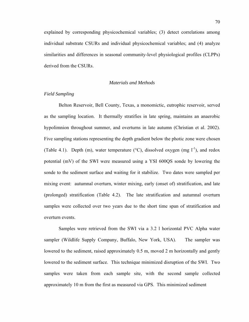
70
explained by corresponding physicochemical variables; (3) detect correlations among
individual substrate CSURs and individual physicochemical variables; and (4) analyze
similarities and differences in seasonal community-level physiological profiles (CLPPs)
derived from the CSURs.
Materials and Methods
Field Sampling
Belton Reservoir, Bell County, Texas, a monomictic, eutrophic reservoir, served
as the sampling location. It thermally stratifies in late spring, maintains an anaerobic
hypolimnion throughout summer, and overturns in late autumn (Christian et al. 2002).
Five sampling stations representing the depth gradient below the photic zone were chosen
(Table 4.1). Depth (m), water temperature (°C), dissolved oxygen (mg l-1), and redox
potential (mV) of the SWI were measured using a YSI 600QS sonde by lowering the
sonde to the sediment surface and waiting for it stabilize. Two dates were sampled per
mixing event: autumnal overturn, winter mixing, early (onset of) stratification, and late
(prolonged) stratification (Table 4.2). The late stratification and autumnal overturn
samples were collected over two years due to the short time span of stratification and
overturn events.
Samples were retrieved from the SWI via a 3.2 l horizontal PVC Alpha water
sampler (Wildlife Supply Company, Buffalo, New York, USA). The sampler was
lowered to the sediment, raised approximately 0.5 m, moved 2 m horizontally and gently
lowered to the sediment surface. This technique minimized disruption of the SWI. Two
samples were taken from each sample site, with the second sample collected
approximately 10 m from the first as measured via GPS. This minimized sediment
71
Table 4.1: Morphometric characteristics of Belton Reservoir and corresponding average depth of each sampling site located within the reservoir.
Location 31° 07' N, 97° 29' WSurface Area (km2) 49.8Volume (x 108 m3) 5.45Secchi Depth (m) 1.2 - 2Mean Depth (m) Whole Lake 10.9 Sampling Site 1 13.7 Sampling Site 2 16.4 Sampling Site 3 20.5 Sampling Site 4 22.8 Sampling Site 5 25.8
resuspension of the first sample affecting the second sample. This sampling scheme was
used to sample the benthic boundary layer. This layer is a component of the sediment-
water interface, often defined as an area of high discontinuity in wet bulk density and
high rates of sinking particles, thus differing from the water column and sediment column
(Austen et al. 2002; Hulbert et al. 2002). Thus the samples were turbid, yet liquid in
consistency. Equal volumes of the duplicate samples from each station (water with
sediment particles) were pooled in a 300-ml dark dissolved oxygen bottle and capped to
maintain in situ dissolved oxygen concentration. The sampler was rinsed with 0.45-μm
filtered and/or deionized water between samples. Samples were held at collected
temperature until returned to the laboratory. Samples were processed within 5 h of
collection.
Laboratory Analyses
Biolog EcoPlates (Biolog, Inc., Hayward, California, USA) were inoculated with
150 μl of pooled sample per well. A single EcoPlate was inoculated for each pooled
sample, with one pooled sample per station. EcoPlates contain each of the 31 substrates

72
Table 4.2: Physicochemical data and bacterial abundance at the sediment-water interface for all sampling sites and dates. Dates are classified based on mixing characteristics of the lake.
Classification Date Site Temperature Dissolved Redox Bacteria(°C) Oxygen (mg l-1) Potential (mV) x 106 ml-1
Late Stratification 16-Oct-03 1 23.7 3.1 225 1.22 17.1 0.6 276 1.03 17.0 0.0 93 5.04 15.5 0.0 38 1.95 14.9 0.0 4 0.6
Fall Overturn 6-Nov-03 1 21.1 3.0 296 1.52 21.0 4.8 364 1.33 21.1 5.5 219 3.04 21.1 5.1 342 1.25 18.6 1.2 103 2.5
Winter Mixing 31-Jan-04 1 11.4 9.7 348 10.52 11.3 10.0 347 5.03 11.4 10.1 367 13.14 11.4 10.6 392 4.05 11.5 10.6 383 6.3
Winter Mixing 12-Mar-04 1 11.8 7.6 384 1.42 11.4 7.1 380 1.33 11.2 7.7 394 1.04 10.9 9.9 391 1.35 10.9 8.6 383 2.2
Early Stratification 6-May-04 1 19.4 8.0 217 1.12 18.8 6.0 231 1.13 17.9 6.9 409 0.74 16.4 2.5 293 0.55 15.1 1.5 255 0.6
Early Stratification 1-Jul-04 1 25.8 4.4 381 1.22 22.9 1.1 258 1.53 21.0 0.4 186 1.04 19.6 0.2 155 1.65 19.4 0.0 120 2.5
Late Stratification 9-Sep-04 1 27.0 2.9 230 1.72 26.8 1.3 157 2.43 23.7 0.8 108 1.94 20.6 0.0 37 1.75 20.1 0.0 15 1.2
Fall Overturn 14-Oct-04 1 24.6 7.4 431 1.12 24.6 7.2 405 1.53 24.6 5.3 411 2.34 24.6 6.8 415 2.25 24.5 6.6 341 3.1

73
in triplicate, thus allowing intraplate replication for each pooled sample. For samples
with dissolved oxygen concentrations less than 0.2 mg l-1, anaerobic inoculation,
processing, and incubation techniques were used as outlined in Chapter Three.
Plates were incubated at 22°C and read at OD590 (i.e. absorption spectrum of the
formazan precipitate) once daily for five days using a Biolog MicroStation 2 plate reader.
22°C was chosen for the incubation temperature, not as an optimum, but to maintain
consistency throughout the experiment. Varying incubation temperatures instead of a pre-
selected incubation temperature may confound spatial and temporal CSUR variation with
differences due to incubation temperature variation (Chapter Three; Christian and Lind
2006).
For each plate, mean OD590 for each carbon substrate at each reading time was
corrected by subtracting the mean OD590 of the control (no substrate) wells at the same
reading time. Subtraction of control wells eliminated color and turbidity effects due to
varying amounts of sediment (clay) particles in the samples. The corrected OD590 for
each substrate was plotted against time. Logistic bacterial growth rates were observed;
therefore a three-parameter sigmoidal curve was fitted to each substrate for each sample
using Sigma Plot 2000. The rate of exponential growth determined by the curve was the
CSUR metric (Lindstrom et al. 1998; Christian and Lind 2006).
In addition to Biolog assays, aliquots of each pooled sample were preserved in
formalin (2% final concentration) for total bacterial enumeration. The bacteria were
stained with DAPI fluorochrome (1 µg ml-1 final concentration), filtered onto 0.2-µm
blackened polycarbonate filters, and viewed under UV excitation at 1500 x
magnification. Total bacteria ml-1 were estimated by counting 20 fields or 300 bacteria
74
per filter (Porter and Feig 1980). For bacteria attached to clay particles, a correction
factor of 2 x was applied (Lind and Dávalos-Lind 1991).
Statistical Analyses
Summary and univariate statistics (i.e. correlation/regression, One-way ANOVA,
Student’s t) were performed using JMP 5.0 and Microsoft Office Excel 2003. A
significance level of α = 0.05 was used. CANOCO 4.5 was used for all multivariate
analyses. CanoDraw for Windows, a graphical analysis package included with
CANOCO 4.5, was used for graphical analyses of the multivariate data.
The complete multivariate data set consisted of four subsets, each subset
including all sites and dates corresponding to a specific season (mixing event). Each
subset consisted of two parts: (1) response (dependent) variables (CSURs) for the 31
substrates (listed in columns) for each corresponding date and site (listed in rows); and
(2) supplemental environmental (independent) variables (i.e. temperature, dissolved
oxygen, redox potential, bacterial abundance) (columns) for each corresponding date and
site (rows). This grouping by subset allowed individual analyses for each mixing event,
and partitioned out the covariable effects of sample site. All CSUR data were centered to
a mean of zero and standardized to unit variance before conducting the multivariate
analyses.
Preliminary data analysis using detrended correspondence analysis (DCA) on the
response (CSUR) data for each subset, detrended by segments, established first gradient
lengths of 1.4 – 2.9 standard deviation units. Gradients less than 2.0 indicate relatively
low beta diversity; hence these data should be subjected to linear ordination methods (e.g.
principal components analysis) rather than unimodal ordination methods (e.g.
75
correspondence analysis). However, gradients ranging from 2.0 – 4.0 work well with
either ordination method (Lepš and Šmilauer 2003). For consistency and comparison
among subsets, principal components analysis (PCA) was used. This analysis extracted
orthogonal linear combinations of variables (principal components) that corresponded to
the maximum amount of variation in the subset. PCA produces as many principal
components as there are variables. However, only significant components are retained
for analyses (ter Braak and Šmilauer 2002).
The environmental variables were projected onto the PCA axes a posteriori to
assess the amount of variation in the PCA data that could be attributed to the
environmental variables. While this approach was indirect, it did not require stringent
assumptions as does direct gradient analyses (e.g. Redundancy Analysis, Canonical
Correspondence Analysis) and therefore precludes the use of significance tests (Grover
and Chrzanowski 2000).
Results
Seasonal Carbon Substrate Utilization Patterns
Figure 4.1 (a – d) shows loadings of SWI bacterial CSURs onto the first two PCA
axes for each seasonal mixing event. Only utilizations that had greater than 50 percent fit
(i.e. significant loadings) onto the two axes collectively were included for interpretation.
Additionally, only the first two PCA axes were retained for interpretation as the other
axes did not account for a significant percentage of the total variance as determined by
application of the broken-stick model (Lepš & Šmilauer, 2003; Peres-Neto et al., 2003).

76
During early summer stratification, the first two PCA axes accounted for 68.2
percent of the total substrate utilization variance. Significant loadings were observed for
15 of the 31 substrates, all strongly positively associated with the first axis and weakly,
but significantly associated with the second axis (Figure 4.1a). These loadings included 9
carbohydrates, 3 carboxylic acids, 2 polymers and 1 amino acid. Hence, carbohydrates
contributed the highest relative utilization by SWI bacteria during early stratification.
-1.0 1.2-1.0
1.0
D4
A2B2
C2D2
E2
G1
H1A3
D3
H3
B1
G2
C1
F1
PCA Axis I (49.8%)
PC
A A
xis
II (1
8.4%
)
-1.0 1.2
-1.0
1.0
A4
D4
E4
F4
E2
D3
E3
F2
F3H3
B1
H2C1
D1 G4
PCA Axis I (46.6%)
PC
A A
xis
II (1
7.2%
)
-1.0 1.2-1.0
1.0
B4
D4
E4F4
A2
B2
C2
D2
G1
H1
D3
E3
G3
B1
G2E1
F1
PCA Axis I (44.6%)
PCA
Axis
II (1
4.1%
)
Figure 4.1(a –d). Principal components analyses showing loadings on principal components axes I and II for substrates that exhibited greater than 50% fit to the axes for early stratification (a), late stratification (b), autumnal overturn (c), and winter mixing (d), respectively. Percent variance explained by each axis is given. Arrows connect at origin. Code numbers correspond to substrates given in Table 1.
A B
C D
77
During late season (prolonged) stratification, measured during two consecutive
years, the first two PCA axes accounted for 63.8 percent of the total substrate utilization
variance. Significant loadings of 15 substrates were observed, all strongly positively
loading onto the first axis and weakly onto the second axis (Figure 4.1b). These loadings
included six carboxylic acids, four amino acids, two polymers, two carbohydrates, and
one amine. Opposite of early stratification, late season stratification was characterized by
the high SWI bacterial utilization of amino acids and carboxylic acids and low utilization
of carbohydrates.
At the onset of autumnal overturn, as measured during two consecutive years,
significant loadings for 17 substrates were observed, all except pyruvic acid methyl ester
explained by high negative loadings on PCA axis I and moderate loadings on axis II
(Figure 4.1c). The first two PCA axes accounted for 58.7 percent of the total variance.
Substrates exhibiting significant loadings included seven carbohydrates, four amino
acids, four carboxylic acids, and two polymers. Because of the negative loadings on the
first axis (which explained 44.6 percent of the substrate utilization variance), these
substrates contributed little to SWI bacterial carbon substrate utilization during overturn,
specifically most carbohydrates and amino acids.
During winter mixing, significant loadings were observed for 15 substrates. The
first two PCA axes accounted for 57.6 percent of the total variance (Figure 4.1d). These
substrates exhibited diverse loadings on both PCA axes. Three carbohydrates and two
polymers exhibited positive loadings on PCA axis I, while two carbohydrates and one
carboxylic acid exhibited positive loadings on PCA axis II. Four carboxylic acids, and a
single carbohydrate, amino acid, and amine display negative loadings on PCA axis II.
78
These data indicate that during cold, mixing conditions carbohydrates and polymers
contributed the highest utilization responses, yet trends were not as defined as during
other seasons.
Carbon Substrate Utilization Variation Attributed to Environmental Variables
While only the first two PCA axes were significant for each seasonal data set,
there are a total of as many PCA axes as there are substrates (n = 31), in total accounting
for 100 percent of the substrate utilization variance. Of this total variance, linear
combinations of measured environmental variables (i.e. bacterial abundance, SWI
temperature, dissolved oxygen, redox potential) were fitted onto the PCA axes a
posteriori to determine the percentage of total variance attributable to the environmental
variables (Table 4.3). For each seasonal mixing event, environmental variables
accounted for no less than 50 percent of the total variance, with the largest percentage
accounted for during autumnal overturn (62.3 percent). Temperature was the largest
attributable variable during early stratification (19.2 percent) and autumnal overturn (40
percent). The largest amount of variation accounted for by dissolved oxygen and redox
potential individually was during autumnal overturn (32.4 and 30.8 percent, respectively)
and the least during late stratification (7.3 and 11 percent, respectively). The relationship
for dissolved oxygen and redox potential individually also held for the combined effect of
dissolved oxygen and redox potential. Their combined effect is more ecologically
interpretable than either variable individually due to their high correlation and
codependence. The sum of the variances of the individual variables was greater than the
total variance explained by the variables collectively due to significant correlations
among several of the variables (Lepš & Šmilauer, 2003).

79
Table 4.3: Percent variance in seasonal CSUR data explained by individual environmental variables and all variables collectively. Sum of percentages of individual variables are greater than percentage of all
variables collectively due to correlation of the individual variables.
Winter Early Fall LateVariable Mixing Stratification Overturn Stratification
All Variables 49.8 54.0 62.3 62.1 Bacteria ml-1 24.0 14.4 5.7 20.5 Temperature ( C ) 6.4 19.2 40.0 16.4 Dissolved Oxygen (mg l-1) 15.1 14.3 32.4 7.3 Redox Potential (mV) 16.1 14.6 30.8 11.0 Oxygen * Redox 13.6 19.9 38.6 6.7
During late season stratification and winter mixing, bacterial abundance
accounted for the largest proportion of the CSUR variance (20.5 and 24 percent,
respectively), while during autumnal overturn it accounted for little variance (5.7
percent). A significant difference was observed among seasonal bacterial abundance
(One-way ANOVA, F3,36 = 4.36, p < 0.01). However, the only pairwise difference was
greater abundance during winter mixing than during early stratification (Tukey’s HSD, q
= 2.69, α = 0.05). While higher bacterial abundance during winter mixing explained a
high percentage of variance, this trend did not hold for all seasons. There was no
significant difference between bacterial abundance during late stratification and autumnal
overturn (Student’s t.05, 9 = 0.06, p = 0.81), yet variance explained by bacterial abundance
was 20.5 and 5.7 percent, respectively.
Carbon Substrate Utilization and Environmental Variable Correlations
Because a large percentage of variance in SWI bacterial substrate utilization was
explained by the measured environmental variables, we explored relationships among
those environmental variables and individual substrates (Table 4.4). These correlations
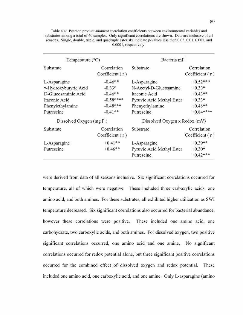
80
Table 4.4: Pearson product-moment correlation coefficients between environmental variables and substrates among a total of 40 samples. Only significant correlations are shown. Data are inclusive of all seasons. Single, double, triple, and quadruple asterisks indicate p-values less than 0.05, 0.01, 0.001, and
0.0001, respectively.
Temperature (°C) Bacteria ml-1
Substrate Correlation Substrate CorrelationCoefficient ( r ) Coefficient ( r )
L-Asparagine -0.46** L-Asparagine +0.52***γ-Hydroxybutyric Acid -0.33* N-Acetyl-D-Glucosamine +0.33*D-Glucosaminic Acid -0.46** Itaconic Acid +0.43**Itaconic Acid -0.58**** Pyruvic Acid Methyl Ester +0.33*Phenylethylamine -0.48*** Phenyethylamine +0.48**Putrescine -0.41** Putrescine +0.84****
Dissolved Oxygen (mg l-1) Dissolved Oxygen x Redox (mV)
Substrate Correlation Substrate CorrelationCoefficient ( r ) Coefficient ( r )
L-Asparagine +0.41** L-Asparagine +0.39**Putrescine +0.46** Pyruvic Acid Methyl Ester +0.30*
Putrescine +0.42***
were derived from data of all seasons inclusive. Six significant correlations occurred for
temperature, all of which were negative. These included three carboxylic acids, one
amino acid, and both amines. For these substrates, all exhibited higher utilization as SWI
temperature decreased. Six significant correlations also occurred for bacterial abundance,
however these correlations were positive. These included one amino acid, one
carbohydrate, two carboxylic acids, and both amines. For dissolved oxygen, two positive
significant correlations occurred, one amino acid and one amine. No significant
correlations occurred for redox potential alone, but three significant positive correlations
occurred for the combined effect of dissolved oxygen and redox potential. These
included one amino acid, one carboxylic acid, and one amine. Only L-asparagine (amino
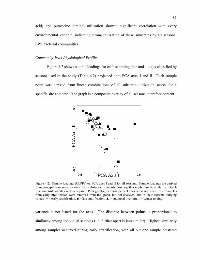
81
acid) and putrescine (amine) utilization showed significant correlation with every
environmental variable, indicating strong utilization of these substrates by all seasonal
SWI bacterial communities.
Community-level Physiological Profiles
Figure 4.2 shows sample loadings for each sampling date and site (as classified by
season) used in the study (Table 4.2) projected onto PCA axes I and II. Each sample
point was derived from linear combinations of all substrate utilization scores for a
specific site and date. The graph is a composite overlay of all seasons; therefore percent
Figure 4.2: Sample loadings (CLPPs) on PCA axes I and II for all seasons. Sample loadings are derived from principal components scores of all substrates. Symbols close together imply sample similarity. Graph is a composite overlay of four separate PCA graphs, therefore percent variance is not listed. Two samples from early stratification were removed from the graph, but not analyses, due to their extreme outlying values. ◊ = early stratification, ■ = late stratification, ▲ = autumnal overturn, ○ = winter mixing.
variance is not listed for the axes. The distance between points is proportional to
similarity among individual samples (i.e. further apart is less similar). Highest similarity
among samples occurred during early stratification, with all but one sample clustered

82
together with low eigenvalues along PCA axis I and high eigenvalues along PCA axis II.
The two furthest outliers from early stratification were excluded from the graph, but not
from analyses, due to their extreme distance away from other samples. High similarity
also occurred during autumnal overturn, even though these samples were collected during
two different years. Lowest similarity was observed during late stratification, with a
wide range of eigenvalues spread along PCA axes I and II. Low similarity was also
observed during winter mixing, explained primarily by PCA axis II.
Discussion
Organic carbon utilization by heterotrophic bacteria strongly influences internal
nutrient cycling in freshwater ecosystems and impacts eutrophication processes
(Sinsabaugh et al. 1997; Qu et al. 2005). Specifically, bacterially-mediated sediment
nutrient releases often input nutrients into the water column at greater quantities than
allochthonous sources (Heinen and McManus 2004; Song et al. 2004). Organic carbon
utilized by heterotrophic bacteria is commonly classified into three groups: particulate
organic carbon (POC), high molecular dissolved organic carbon (HM-DOC), and low
molecular dissolved organic carbon (LM-DOC) (Wirtz 2003). This investigation
specifically explored SWI bacterial utilization of the LM-DOC via the use of Biolog
EcoPlates. CSUR data generated from the EcoPlates represents bacterial community
functional potential and has been used to assess functional ability and changes in various
environmental bacterial communities (Garland 1997; Preston-Mafham et al. 2002). By
considering the limitations of EcoPlates (i.e. inoculum density, incubation temperature,
oxygen contamination) and modifying our protocol to avoid these limitations (i.e. using
83
growth rate metrics, incubation temperature standardization, anaerobic techniques),
results were robustly interpreted (see Chapter Three).
Seasonal Carbon Substrate Use
Few explanations for preferential seasonal use of DOC substrates by freshwater
(specifically, SWI) bacteria have been proposed (Pettine et al. 1999; Brugger et al. 2001)
therefore this investigation served an exploratory, not confirmatory purpose. Future
investigations (i.e. in situ chemical measurements; stable isotope analysis) into the
presence or absence of these substrates at the SWI will aid the results obtained in this
study. Most substrates in the Biolog EcoPlates were used at various extents during all
seasons; however the first two PCA axes for each seasonal data subset shows only those
substrates that contributed to significant variation in increased and/or decreased substrate
utilization. Therefore different seasonal patterns of SWI bacterial substrate use were
elucidated from the PCA graphs (Figure 4.1a-d).
During the onset of spring stratification, characterized by warming temperatures
and depletion of dissolved oxygen and decreasing redox potential, SWI bacterial
assemblages preferentially used carbohydrates over carboxylic acids, amino acids, and
amines. As summer stratification progressed (i.e. late season stratification), indicated by
warm temperatures and depleted dissolved oxygen and reduced redox potential, substrate
preference shifted to amino acids, carboxylic acids, and amines with little use of
carbohydrates. At the onset of autumnal overturn marked by decreasing temperatures,
replenishment of dissolved oxygen, increasing (oxidized) redox potentials and presence
of turbulent mixing, SWI bacteria decreased use of amino acids and continued little use
84
of carbohydrates. Throughout winter mixing, SWI bacteria had high preference for
carbohydrates and polymers.
Highest carbohydrate use during early stratification, along with high
carbohydrate use during winter mixing may suggest that SWI bacterial communities
prefer carbohydrate substrates under oxic conditions and pre-anoxia, under a wide variety
of temperatures. Indeed, the preferred catabolic pathway of many aerobic and facultative
heterotrophs involves oxidation of a simple or complex carbohydrate and oxygen as a
terminal electron acceptor (Madigan et al. 1997; Rosenstock and Simon 2003). In
addition, fixed carbon in the form of carbohydrates synthesized via phytoplankton
photosynthesis and carbohydrate-rich allochthonous organic matter is flushed in and
sinks to sediments during lake mixing (Vreča 2003; Heinen and McManus 2004); hence
conditions present during winter mixing may select for SWI bacterial populations that
readily utilize carbohydrates. Lowest carbohydrate utilization during late season
stratification and onset of autumnal overturn are possibly attributed to SWI carbohydrate
depletion from lack of mixing combined with high hypolimnetic bacterial activity that
oxidizes sinking carbohydrates before they can reach the sediments (Cole and Pace 1995;
Seiter et al. 2005).
Amino acids were preferentially used during late stratification. Amino acids were
used to a much lesser extent during autumnal overturn, winter mixing, and onset of
stratification. Unlike carbohydrates and carboxylic acids, amino acids are nitrogen-rich
(Madigan et al. 1997). Thus SWI bacteria may utilize amino acids as a nitrogen, in
addition to a carbon, source by assimilating the ammonium side-chain (Pettine et al.
1999). In turn, the ammonium is incorporated into organic molecules such as other
85
amino acids and proteins (Hollibaugh and Azam 1983). High use of amino acids
suggests that bacteria may be nitrogen deprived during late stratification, even though
during this time ammonium is produced from bacterial nitrate reduction. Thus nitrogen
deprivation at the SWI during late stratification may result from decreased sinking of
nitrogen-rich organic matter due to lack of reservoir mixing (Hodell and Schelske 1998).
Because of the opposing catabolic and anabolic processes of amino acid utilization, the
breakdown of these extracellular amino acids and incorporation into cellular amino acids
may be performed by separate bacterial taxa in a synergistic interaction rather than both
processes conducted simultaneously by the same taxon (Atlas & Bartha 1998). In
addition, previous studies on Lake Belton have indicated that larger bacteria are present
during late summer stratification and their size is a function of anoxia (Christian et al.
2002); hence the larger bacteria may require a greater number of enzymes and proteins
for metabolic functions, which can be synthesized via uptake of ammonium from amino
acid breakdown in the environment.
Carboxylic acid utilization was greatest during late season stratification, but also
had marked utilization during other seasons. Of the EcoPlate substrates, the carboxylic
acids are the most diverse substrates in terms of molecular weight and chemical
configuration. Little is known about free carboxylic (organic) acids in aquatic and
sediment systems. Naturally occurring organic acids such as carboxylic acids are often a
product of bacterial fatty acid catabolism, photochemical degradation of HM-DOC, or as
an end product of fermentative metabolism which occurs independent of dissolved
oxygen and redox potential (Bertilsson and Tranvik 2000; Ding and Sun 2005). Studies
at SWIs in marine systems have shown that organic acids degrade more quickly under
86
aerobic than anaerobic conditions and their concentrations are unrelated to bacterial
abundance (Ding and Sun 2005). However, the results show highest utilization of
carboxylic acids during anaerobic, reducing conditions of late stratification. Two
possible reasons for this phenomenon are suggested: (1) increased photoperiod during
late stratification increases photodegradation of HM-DOC and POC in the photic zone,
increasing the amount of organic acid-rich DOC that sinks to the SWI, possibly selecting
for organic acid-utilizing bacteria (Tranvik et al. 1999); (2) fermentative bacteria may be
more prevalent during anoxic conditions, which require the use of an organic compound,
such as a carboxylic acid as an electron acceptor in a fermentative pathway (Madigan et
al. 1997).
Selective Pressures on SWI Bacterial Assemblages
Several SWI environmental (physicochemical and biological) variables exhibited
seasonal change, including: temperature, dissolved oxygen, redox potential and bacterial
abundance. Thus Beijerinck’s adage was invoked, ‘everything is everywhere, the
environment selects’ when assessing these variables affects on CSUR variance, hence the
environmental selective pressures upon SWI bacterial assemblages. While the EcoPlates
were themselves selective, the measured environmental variables collectively were
associated with at least 50 percent of the total CSUR variance each season, thus were
influential environmental selectors for the SWI bacterial assemblages (Table 4.3).
During seasons marked by high variance explained by bacterial abundance, not
just abundance, but also, bacterial per-cell activity (i.e. ability to utilize substrate) may
attribute to this variance. A previous study on Belton Reservoir SWI bacterial
87
communities showed that specific per-cell activity varies on a seasonal basis, supporting
this evidence (see Chapter Two).
The SWI exhibited wide seasonal temperature variation. The highest amount of
CSUR variance explained by temperature was during autumnal overturn, while the lowest
was during winter mixing. CSUR variance due to temperature differences was
proportional to the temperature range exhibited during that season; with the large CSUR
variance during autumnal overturn corresponding to a wide temperature range (18.6°C –
24.6°C) and the small variance during winter mixing corresponding to a small
temperature range (10.9°C – 11.8°C). All plates were incubated at 22°C to maintain
consistency throughout duration of the experiment. However this incubation temperature
may have affected SWI bacterial growth rates, but presumably not pattern (Grover and
Chrzanowski 2000). Therefore CSUR variance due to temperature was a function of
collected temperature as well as the normalized temperature of incubation (22°C).
At the SWI, dissolved oxygen depletion was coupled with lowered redox
potential; therefore their effects upon CSUR variance are best understood when
considered in tandem. The combined effect accounted for the largest percentage of
CSUR variance during autumnal overturn. It also accounted for a large percentage of
CSUR variance during early stratification. These seasons had the greatest ranges of
dissolved oxygen and redox potential. Large redox potential changes are defined by
bacteria that utilize various electron acceptors, implying tremendous changes in SWI
bacterial community composition (Sweerts et al. 1991). Autumnal overturn and early
stratification had the combined effect of dissolved oxygen and redox potential working in
88
reverse for their respective seasons. Therefore it was not surprising that CSUR variance
also showed an opposite relationship (Figure 4.1a and 4.1c).
Individual Substrate Utilization and Environmental Variable Correlations
Individual substrates whose CSUR was significantly positively or negatively
correlated with the individual physicochemical variables were assessed, all seasons
inclusive. Carbohydrates showed strong utilization during two seasons marked by a wide
variation in physicochemical variables (early stratification and winter mixing); therefore
no individual carbohydrate CSUR was significantly correlated with any environmental
variable. Most significant correlations occurred with carboxylic acids (Table 4.4),
possibly due to their highest utilization during a single season marked by similar
physicochemical conditions (late stratification). Interestingly, two substrates were
correlated with all measured environmental variables. These substrates were L-
asparagine (amino acid) and putrescine (amine). Positive correlations of these substrates
CSURs occurred with bacterial abundance, dissolved oxygen, and the combined effect of
dissolved oxygen and redox potential. Negative correlations occurred with temperature.
These two substrates are characterized by low C/N ratios. However, a significant trend
was not observed with every low C/N ratio substrate. Yet a recent study utilizing
EcoPlates demonstrated a preferential utilization of high nitrogen-containing substrates
by bacteria in marine aquatic environments (Sala et al. 2006).
Community-level Physiological Profiles
In addition to individual CSURs, Biolog plates have been used to profile total
bacterial community similarities (Mills and Garland 2002). Applying this to our data
89
(Figure 4.2), highest SWI bacterial community similarities occurred during early
stratification and autumnal overturn, while lowest similarity occurred during winter
mixing and late stratification. High similarity in the autumnal overturn samples was
unexpected because sampling events were conducted during two separate years. This
evidence suggests possible similar SWI bacterial community succession occurs during
overturn. However, late stratification samples were also collected during consecutive
sampling years and exhibited high dissimilarity. Yet, some late stratification samples
from the first year were more similar to samples collected during the second year than
samples collected during the same year. Such seasonal succession in aquatic bacteria has
been observed among differing temperate lakes (Grover and Chrzanowski 2000).
Conclusions
This investigation explored differences among SWI bacterial CSURs, CLPPs, and
several related environmental variables throughout seasonal mixing, stratification, and
anoxia in a eutrophic lake. Using Biolog EcoPlates, distinct seasonal shifts in CSURs
were observed. Seasonal differences in SWI bacterial abundance, temperature, dissolved
oxygen and redox potential accounted for a large percentage of CSUR variance.
Preferential use of amino acids during late summer stratification suggests seasonal SWI
nitrogen limitation. Seasonal similiarity of CLPPs from two separate years suggest a
possible predictable succession of SWI bacterial communities, a phenomenon still poorly
understood among aquatic bacterial communities. While many steadfast conclusions
cannot be obtained from Biolog assays, these data contribute to the ever expanding
knowledge of carbon cycling in aquatic ecosystems and relays the importance of SWIs
and their associated biota to the understanding of lake ecosystem nutrient dynamics and
90
processes. Future investigation into reservoir SWI bacterial dynamics can integrate these
findings into developing specific carbon cycling models and establishing in situ carbon
measurements utilizing a variety of other tools.
Acknowledgments
This work was made possible by the Jack G. and Norma Jean Folmar Research
Grant, Baylor University. We thank Dr. Rene Massengale for the use and instruction of
the Biolog Microstation and related equipment. We also thank Dr. Ryan King and Dr.
Darrell Vodopich for statistical assistance and manuscript criticism. Valuable assistance
in field collection was provided by Christopher Filstrup and David Clubbs.
91
CHAPTER FIVE
Organic Matter at the Sediment-Water Interface of a Stratified, Eutrophic Reservoir:
Sources, Fates, and Stoichiometry
Introduction Organic matter (OM) in reservoirs is produced and supplied by various
autochthonous and allochthonous sources (Dean and Gorham 1998). Much of this OM is
assimilated or oxidized by microorganisms in the water column. The remaining OM
sinks to the sediment-water interface (SWI) where further microbial assimilation and
oxidation of OM occurs, often at significantly higher rates than the overlying water
column (Heinen and McManus 2004). These SWI microbial (i.e. bacterial) processes are
often accompanied by additional nutrient transformations that release nitrogen,
phosphorus, and sulfur-containing compounds into the water column (Nealson 1997).
These nutrients (e.g. ammonia, hydrogen sulfide) contribute to reservoir eutrophication
and aesthetic problems (Nealson and Stahl 1997). Therefore SWI OM sources and fates
are important in the overall carbon budgets and nutrient dynamics of reservoirs.
However, SWI contributions to reservoir OM cycling are less understood than open-
water OM dynamics (Syväranta et al. 2006).
Stratified reservoir mixing events may profoundly influence OM sinking rates to
the SWI, affecting the OM that deposits in sediments (Beutel 2003). In addition, SWI
bacterial metabolism is dependent upon reservoir mixing and stratification (see Chapter
Two). Hence seasonal oxic and anoxic cycles may affect rates of SWI bacterial OM
degradation, as well as the types and fraction (i.e. carbon, nitrogen) of OM degraded.
92
During winter mixing, the total organic carbon (TOC) fraction of SWI OM is
transformed and/or oxidized by aerobic and/or facultative anaerobic heterotrophic
bacteria (Rosenstock et al. 2005). These bacteria utilize oxygen, provided to the SWI via
mixing, as a terminal electron acceptor in respiratory pathways (Ding and Sun 2005).
During warm and tranquil weather conditions, thermal stratification develops between
shallow and deeper waters thus bacteria consume the remaining dissolved oxygen in the
hypolimnion, resulting in an anoxic hypolimnion that blankets the SWI (Bloesch 2004).
As a result, active SWI bacterial assemblages utilize electron acceptors other than oxygen
(e.g. facultative anaerobes, strict anaerobes), or undergo fermentative metabolism. This
may also alter the type and quantity of OM at the SWI.
Overall, sources and fates of carbon and nitrogen are important indicators of
reservoir productivity and trophic dynamics. However, measures of C and N inputs and
quantities at SWIs of reservoirs remains poorly understood. In this investigation total
bulk OM, total inorganic and organic carbon (Cin and Corg) and total nitrogen (Ntot) were
measured at the SWI of a monomictic, eutrophic reservoir on a seasonal and spatial basis.
Relationships among these nutrient concentrations were examined in addition to C/N
ratios and Corg and Ntot stable isotopic signatures (δ13Corg and δ15Ntot). These data
provided seasonal and spatial SWI stoichiometric profiles and isotope signatures of SWI
OM that were defined by OM inputs and SWI bacterial metabolism. Spatially differing
δ13C values of organic carbon (δ13Corg) were used to suggest possible sources of SWI OM
inputs, while temporally differing δ15N values of nitrogen were used to suggest seasonal
changes in SWI OM sources as well as bacterial nitrate utilizations (Lehmann et al.
2002).
93
Materials and Methods
Study Site and Physicochemical Variables Belton Reservoir, a subtropical monomictic and eutrophic reservoir located in
central Texas, was the study location (Figure 1.1). The lacustrine region thermally
stratifies during late spring and develops an anoxic hypolimnion that decreases in redox
potential throughout summer. Thermal mixing begins in mid-autumn and persists
throughout winter (Chapters 2, 3, 4). Reservoir depth varies approximately ± 2 m
depending on the amount of rainfall, inflow, discharge, and water consumption. The
reservoir basin is defined by steep limestone cliffs and little emergent vegetation.
Sediments are clay-rich.
SWI samples were collected from five sites along a longitudinal linear transect
representing the depth gradient of the lacustrine region (Figure 1.2, Table 4.3). Hence,
each site was not equally spaced apart; however each site was separated by a horizontal
distance of at least 200 m. The depth of the hypolimnion blanketing these sites during
summer stratification varied on a spatial and temporal basis. Therefore, this sampling
design provided variability in SWI physicochemical variables (e.g. dissolved oxygen, pH,
redox potential) under a variety of stratification conditions, ranging from weakly
stratified (Site A) to stratified and anoxic (Site E) during summer. Likewise, all sites
underwent overturn in sequential order from Site A to Site E. Samples were collected
from October 2003 through February 2005 during periods of stratification, autumnal
overturn, and winter mixing.
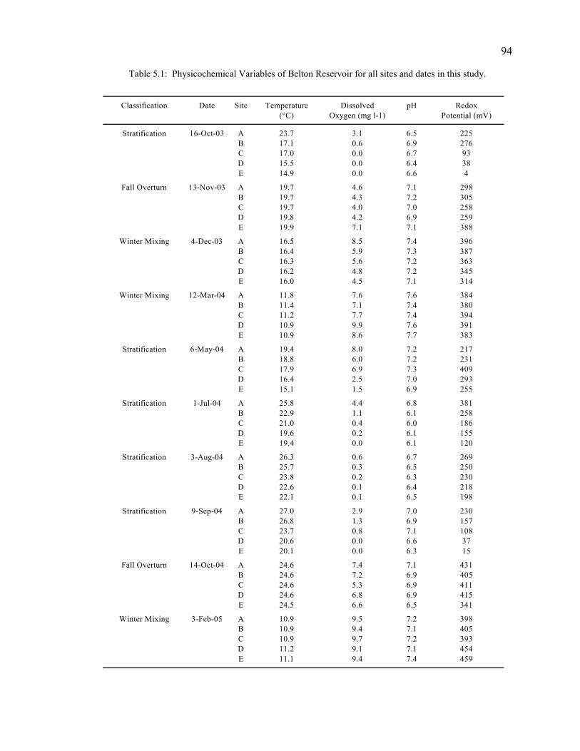
94
Table 5.1: Physicochemical Variables of Belton Reservoir for all sites and dates in this study.
Classification Date Site Temperature Dissolved pH Redox(°C) Oxygen (mg l-1) Potential (mV)
Stratification 16-Oct-03 A 23.7 3.1 6.5 225B 17.1 0.6 6.9 276C 17.0 0.0 6.7 93D 15.5 0.0 6.4 38E 14.9 0.0 6.6 4
Fall Overturn 13-Nov-03 A 19.7 4.6 7.1 298B 19.7 4.3 7.2 305C 19.7 4.0 7.0 258D 19.8 4.2 6.9 259E 19.9 7.1 7.1 388
Winter Mixing 4-Dec-03 A 16.5 8.5 7.4 396B 16.4 5.9 7.3 387C 16.3 5.6 7.2 363D 16.2 4.8 7.2 345E 16.0 4.5 7.1 314
Winter Mixing 12-Mar-04 A 11.8 7.6 7.6 384B 11.4 7.1 7.4 380C 11.2 7.7 7.4 394D 10.9 9.9 7.6 391E 10.9 8.6 7.7 383
Stratification 6-May-04 A 19.4 8.0 7.2 217B 18.8 6.0 7.2 231C 17.9 6.9 7.3 409D 16.4 2.5 7.0 293E 15.1 1.5 6.9 255
Stratification 1-Jul-04 A 25.8 4.4 6.8 381B 22.9 1.1 6.1 258C 21.0 0.4 6.0 186D 19.6 0.2 6.1 155E 19.4 0.0 6.1 120
Stratification 3-Aug-04 A 26.3 0.6 6.7 269B 25.7 0.3 6.5 250C 23.8 0.2 6.3 230D 22.6 0.1 6.4 218E 22.1 0.1 6.5 198
Stratification 9-Sep-04 A 27.0 2.9 7.0 230B 26.8 1.3 6.9 157C 23.7 0.8 7.1 108D 20.6 0.0 6.6 37E 20.1 0.0 6.3 15
Fall Overturn 14-Oct-04 A 24.6 7.4 7.1 431B 24.6 7.2 6.9 405C 24.6 5.3 6.9 411D 24.6 6.8 6.9 415E 24.5 6.6 6.5 341
Winter Mixing 3-Feb-05 A 10.9 9.5 7.2 398B 10.9 9.4 7.1 405C 10.9 9.7 7.2 393D 11.2 9.1 7.1 454E 11.1 9.4 7.4 459

95
SWI temperature (°C), dissolved oxygen (mg l-1), pH, and redox potential (mV),
were measured at the SWI using a YSI QS 600 Data Sonde (Table 5.1). Measurements
were taken by gently lowering the sonde to the sediment surface and allowing
measurements to stabilize. Though SWI physicochemical gradients differed on milli and
micrometer scale, the sonde measurements were representative of the overall
physicochemical conditions that blanketed the sediment surface.
Microcosm Incubations for Determination of SWI Layer Bulk sediment and water were retrieved from the five sample sites during winter
mixing via a Peterson grab sampler and a 3.2 l PVC Alpha water sampler, respectively.
Sediments from all sites were combined in a single deionized water-rinsed mixing tub,
returned to the laboratory, and thoroughly homogenized. Water was stored in deionized
water-rinsed 4 l plastic bottles, returned to the laboratory, combined and mixed in a 5
gallon carboy. One hundred 250 ml glass jars were filled with 150 ml of homogenized
sediment and topped off with mixed sample water. The jars were sealed with lids and
holes were drilled in 50 of the jar lids to allow aerobic incubation. The remaining 50 jars
were wrapped with parafilm to allow anaerobic incubation. All jars were incubated for 1
month in the dark at 20ºC (approximately annual median hypolimnetic temperature) to
allow a stable SWI bacterial community to establish.
After incubation, the 50 aerobic samples were randomly divided into groups of
10. Ten samples served as controls (mean ± s.d. dissolved SWI oxygen concentration
8.6±1.2 mg l-1). The other groups of samples were purged with nitrogen gas to establish
a SWI dissolved oxygen concentration of 4, 2, 1, or 0 mg l-1, respectively as measured by
an Orion model 97-08 dissolved oxygen electrode. Samples were resealed and re-
96
incubated for 24 hours. For the 50 anaerobic samples (all samples dissolved oxygen ≤
0.1 mg l-1), ten samples served as controls while other groups of 10 samples were purged
with oxygen to obtain a dissolved oxygen concentration of 1, 2, 4, and 8 mg l-1,
respectively. These samples were resealed and re-incubated for 24 hours.
After the 24 hour incubation, a Unisense© RD-10 redox electrode was used to
measure the sediment depth (mm) in each sample at which the lowest redox potential
(mV) occurred. The average depth of the lowest redox potential (< 0 mV) in the aerobic
samples (i.e. samples purged with dissolved oxygen) was approximately 11 mm, while
this depth for anaerobic samples (i.e. samples purged with nitrogen) was approximately 9
mm. Henceforth these depths were used to define the SWI, with 10 mm being the depth
that all future collected samples were subsampled for all analyses.
Sediment-Water Interface Sampling and Storage SWI samples were retrieved via a 15 cm x 15 cm Ekman dredge, modified to
minimize SWI disruption. Three samples were collected per site on each date listed n
Table 5.1. Immediately upon retrieval, excess water was gently siphoned away from the
sediment surface, leaving approximately 1 cm of water overlay. Liquid nitrogen was
slowly poured into a corner of the dredge to freeze the sediment into a solid block being
careful to maintain SWI integrity and composition. The frozen sediment block was
gently removed from the dredge, wrapped in aluminum foil, bagged in plastic, and placed
into a cooler of dry ice. The frozen blocks were returned to the laboratory and held at -
80°C until further processing.
97
Sediment Processing The frozen sediment blocks were subsampled with a scalpel to a depth of
approximately 10 mm. This 10 mm sediment layer was thawed and homogenized in a 50
ml plastic conical centrifuge tube. The samples were held at -30°C until further
processing.
Total Organic Matter Quantification Approximately 10-20 g of the thawed and homogenized sediment was added to a
pre-weighed crucible, dried at 100°C for 24 h, and pulverized to a fine powder. Percent
water was calculated as the difference between wet mass (gram wet weight (gww)) and
dry mass (gram dry weight (gdw)) divided by gww. Approximately 2 g of the powdered
sediment was preserved for carbon and nitrogen analysis and stable isotope analysis. The
remaining powdered sediment was ignited in a crucible at 550°C for 1 hour. Loss on
ignition (LOI) was recorded as the difference between the mass of the dried sample and
the ignited (ashed) sample. Percent TOM was calculated as the LOI divided by gram dry
weight (Dean 1974).
Carbon and Nitrogen Content Approximately 30 mg of dried, but not ashed, sediment samples were measured
into tin capsules and analyzed for total carbon (Ctot) and total nitrogen (Ntot) on a
ThermoQuest Flash EA™ 1112 Elemental Analyzer. 30 mg aliquots of ashed sediments
were analyzed via the same process for total inorganic carbon (Cin). Total organic carbon
(Corg) was calculated as the difference between Ctot and Cin. No inorganic nitrogen was
present in the samples; therefore Ntot was equal to total organic nitrogen. C/N ratios were
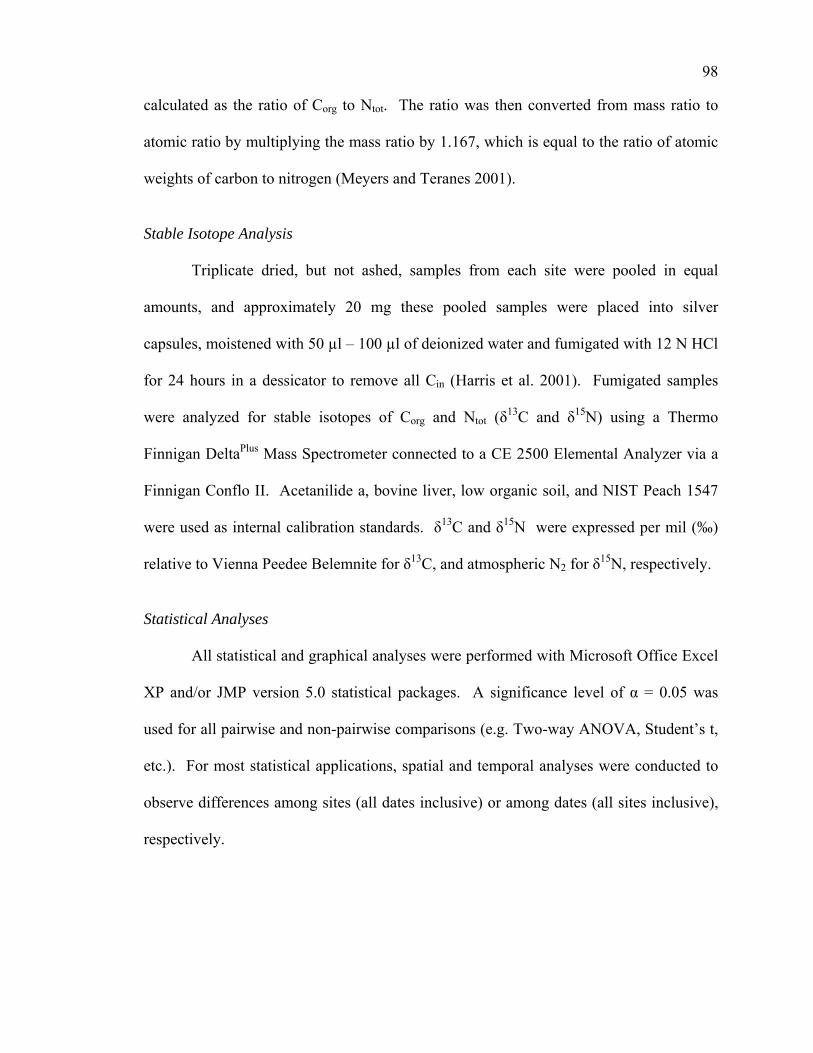
98
calculated as the ratio of Corg to Ntot. The ratio was then converted from mass ratio to
atomic ratio by multiplying the mass ratio by 1.167, which is equal to the ratio of atomic
weights of carbon to nitrogen (Meyers and Teranes 2001).
Stable Isotope Analysis Triplicate dried, but not ashed, samples from each site were pooled in equal
amounts, and approximately 20 mg these pooled samples were placed into silver
capsules, moistened with 50 µl – 100 µl of deionized water and fumigated with 12 N HCl
for 24 hours in a dessicator to remove all Cin (Harris et al. 2001). Fumigated samples
were analyzed for stable isotopes of Corg and Ntot (δ13C and δ15N) using a Thermo
Finnigan DeltaPlus Mass Spectrometer connected to a CE 2500 Elemental Analyzer via a
Finnigan Conflo II. Acetanilide a, bovine liver, low organic soil, and NIST Peach 1547
were used as internal calibration standards. δ13C and δ15N were expressed per mil (‰)
relative to Vienna Peedee Belemnite for δ13C, and atmospheric N2 for δ15N, respectively.
Statistical Analyses All statistical and graphical analyses were performed with Microsoft Office Excel
XP and/or JMP version 5.0 statistical packages. A significance level of α = 0.05 was
used for all pairwise and non-pairwise comparisons (e.g. Two-way ANOVA, Student’s t,
etc.). For most statistical applications, spatial and temporal analyses were conducted to
observe differences among sites (all dates inclusive) or among dates (all sites inclusive),
respectively.
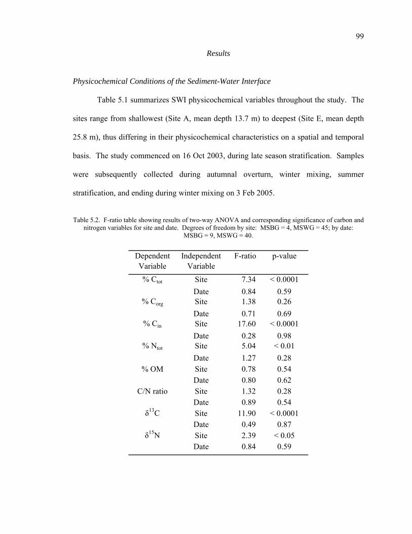
99
Results Physicochemical Conditions of the Sediment-Water Interface
Table 5.1 summarizes SWI physicochemical variables throughout the study. The
sites range from shallowest (Site A, mean depth 13.7 m) to deepest (Site E, mean depth
25.8 m), thus differing in their physicochemical characteristics on a spatial and temporal
basis. The study commenced on 16 Oct 2003, during late season stratification. Samples
were subsequently collected during autumnal overturn, winter mixing, summer
stratification, and ending during winter mixing on 3 Feb 2005.
Table 5.2. F-ratio table showing results of two-way ANOVA and corresponding significance of carbon and
nitrogen variables for site and date. Degrees of freedom by site: MSBG = 4, MSWG = 45; by date: MSBG = 9, MSWG = 40.
Dependent Independent F-ratio p-valueVariable Variable% Ctot Site 7.34 < 0.0001
Date 0.84 0.59% Corg Site 1.38 0.26
Date 0.71 0.69% Cin Site 17.60 < 0.0001
Date 0.28 0.98% Ntot Site 5.04 < 0.01
Date 1.27 0.28% OM Site 0.78 0.54
Date 0.80 0.62C/N ratio Site 1.32 0.28
Date 0.89 0.54δ13C Site 11.90 < 0.0001
Date 0.49 0.87δ15N Site 2.39 < 0.05
Date 0.84 0.59
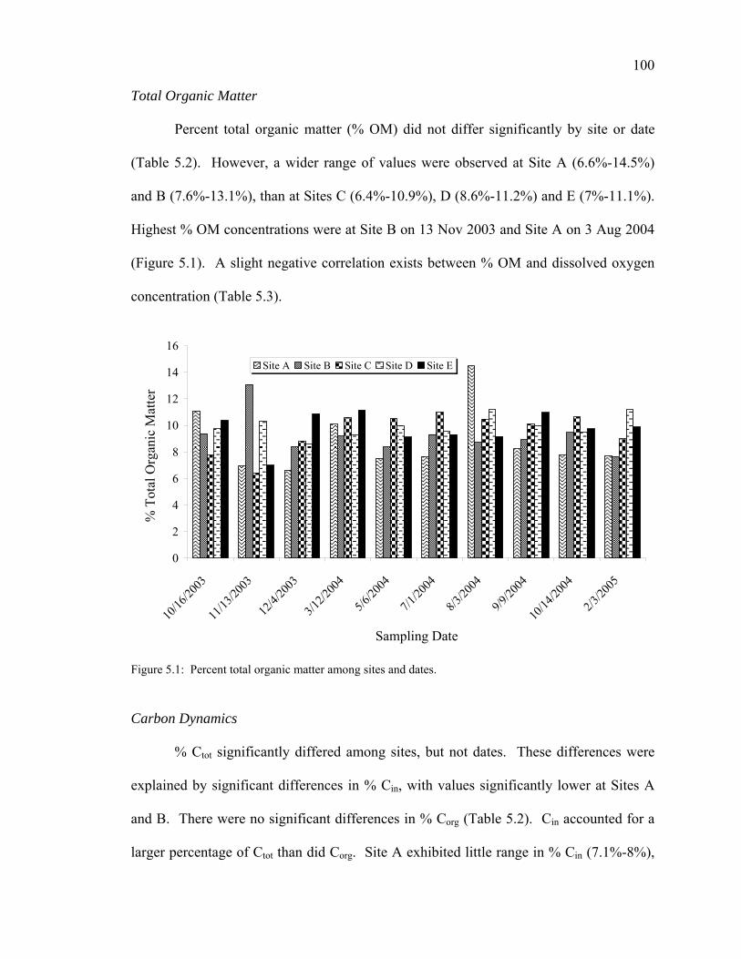
100
Total Organic Matter
Percent total organic matter (% OM) did not differ significantly by site or date
(Table 5.2). However, a wider range of values were observed at Site A (6.6%-14.5%)
and B (7.6%-13.1%), than at Sites C (6.4%-10.9%), D (8.6%-11.2%) and E (7%-11.1%).
Highest % OM concentrations were at Site B on 13 Nov 2003 and Site A on 3 Aug 2004
(Figure 5.1). A slight negative correlation exists between % OM and dissolved oxygen
concentration (Table 5.3).
0
2
4
6
8
10
12
14
16
10/16
/2003
11/13
/2003
12/4/
2003
3/12/2
004
5/6/20
04
7/1/20
04
8/3/20
04
9/9/20
04
10/14
/2004
2/3/20
05
Sampling Date
% T
otal
Org
anic
Mat
ter
Site A Site B Site C Site D Site E
Figure 5.1: Percent total organic matter among sites and dates. Carbon Dynamics
% Ctot significantly differed among sites, but not dates. These differences were
explained by significant differences in % Cin, with values significantly lower at Sites A
and B. There were no significant differences in % Corg (Table 5.2). Cin accounted for a
larger percentage of Ctot than did Corg. Site A exhibited little range in % Cin (7.1%-8%),

101
as did Site B (6.3%-7.3%) and Site C (6.4%-7.5%). Site D (4.7%-6.9%) and Site E
(4.6%-6.4%) exhibited wider ranges of % Cin (Figure 5.2). % Ctot was weakly, but
positively correlated with SWI temperature, while % Corg and % Cin were not
significantly correlated with any measured physicochemical variables (Table 5.3).
However, % Corg and % Cin were negatively correlated with each other (Table 5.4).
Table 5.3: Pearson product-moment correlations and corresponding p-values for carbon and nitrogen
correlations with various physicochemical variables. Significant values occur at p < 0.05.
Variable Temperature Dissolved O2 p H Redox Potential (°C) (mg l-1) (mV)
r p-value r p-value r p-value r p-value
% Ctot 0.26 0.05 0.10 0.35 0.14 0.38 0.03 0.81 % Corg 0.07 0.62 0.17 0.24 0.20 0.16 0.02 0.86 % Cin 0.22 0.11 0.00 0.98 0.03 0.83 0.02 0.91 % Ntot 0.08 0.55 -0.37 0.01 -0.36 0.01 0.20 0.15 % OM 0.06 0.64 -0.25 0.05 0.20 0.17 0.14 0.35
C/N ratio 0.01 0.97 0.04 0.76 0.01 0.91 0.20 0.14 δ13C 0.10 0.44 0.10 0.41 0.06 0.65 0.10 0.48 δ15N 0.02 0.89 -0.24 0.09 0.20 0.19 0.20 0.15
Table 5.4: Significant Pearson product-moment correlations and corresponding p-values between carbon and nitrogen variables.
Correlation r p-value
% Ctot & % Ntot 0.41 < 0.01% Ctot & C/N ratio 0.26 < 0.05% Ctot & δ13C 0.30 < 0.05% Corg & % OM 0.32 < 0.05% Corg & % Cin -0.32 < 0.05% Corg & % Ntot 0.36 < 0.01% Cin & C/N ratio -0.42 < 0.01% OM & % Ntot 0.28 < 0.05δ13C & % Ntot -0.39 < 0.01
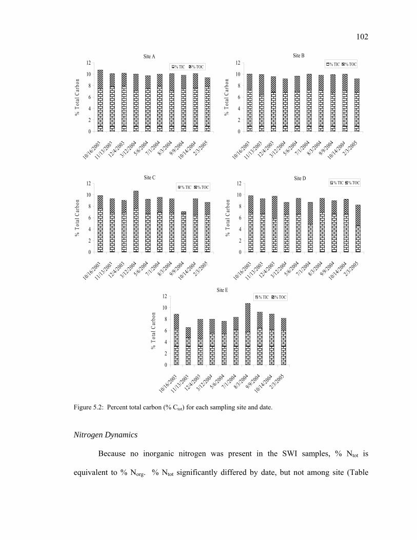
102
Site A
0
2
4
6
8
10
12
10/16/2003
11/13/2003
12/4/2003
3/12/2004
5/6/2004
7/1/2004
8/3/2004
9/9/2004
10/14/2004
2/3/2005
% T
otal
Car
bon
% TIC % TOC
Site B
0
2
4
6
8
10
12
10/16/2003
11/13/2003
12/4/2003
3/12/2004
5/6/2004
7/1/2004
8/3/2004
9/9/2004
10/14/2004
2/3/2005
% T
otal
Car
bon
% TIC % TOC
Site C
0
2
4
6
8
10
12
10/16/2003
11/13/2003
12/4/2003
3/12/2004
5/6/2004
7/1/2004
8/3/2004
9/9/2004
10/14/2004
2/3/2005
% T
otal
Car
bon
% TIC % TOC
Site D
0
2
4
6
8
10
12
10/16/2003
11/13/2003
12/4/2003
3/12/2004
5/6/2004
7/1/2004
8/3/2004
9/9/2004
10/14/2004
2/3/2005
% T
otal
Car
bon
% TIC % TOC
Site E
0
2
4
6
8
10
12
10/16/2003
11/13/2003
12/4/2003
3/12/2004
5/6/2004
7/1/2004
8/3/2004
9/9/2004
10/14/2004
2/3/2005
% T
otal
Car
bon
% TIC % TOC
Figure 5.2: Percent total carbon (% Ctot) for each sampling site and date. Nitrogen Dynamics
Because no inorganic nitrogen was present in the SWI samples, % Ntot is
equivalent to % Norg. % Ntot significantly differed by date, but not among site (Table

103
5.2). When all SWI sites were categorized as ‘stratified’ or ‘mixing’, a significant
difference existed between % Ntot for these groupings (Student’s t = -2.07, p < 0.05).
Large fluctuations were observed among many % Ntot concentrations, some dates
exhibiting similar or identical values at several sites (e.g. 4 Dec 2003; 8 Aug 2004),
others exhibiting a wide range of values (e.g. 13 Nov 2003; 1 Jul 2004) (Figure 5.3). %
Ntot was negatively correlated to both dissolved oxygen and pH (Table 5.3). Significant
positive correlations occurred between % Ntot and % Ctot; % Ntot and % Corg; and % Ntot
and % OM (Table 5.4).
0.18
0.24
0.3
0.36
0.42
10/16
/2003
11/13
/2003
12/4/
2003
3/12/2
004
5/6/20
04
7/1/20
04
8/3/20
04
9/9/20
04
10/14
/2004
2/3/20
05
% N
tot
Site A Site B Site CSite D Site E
Figure 5.3: Percent total nitrogen (%Ntot) at each site throughout the course of the study. Carbon to Nitrogen Ratios
SWI C/N ratios (% Corg atomic / % Ntot atomic) did not significantly differ by site
or date (Table 5.2), nor were the ratios significantly correlated to any measured
physicochemical variable (Table 5.3). On several dates, C/N ratios were similar among
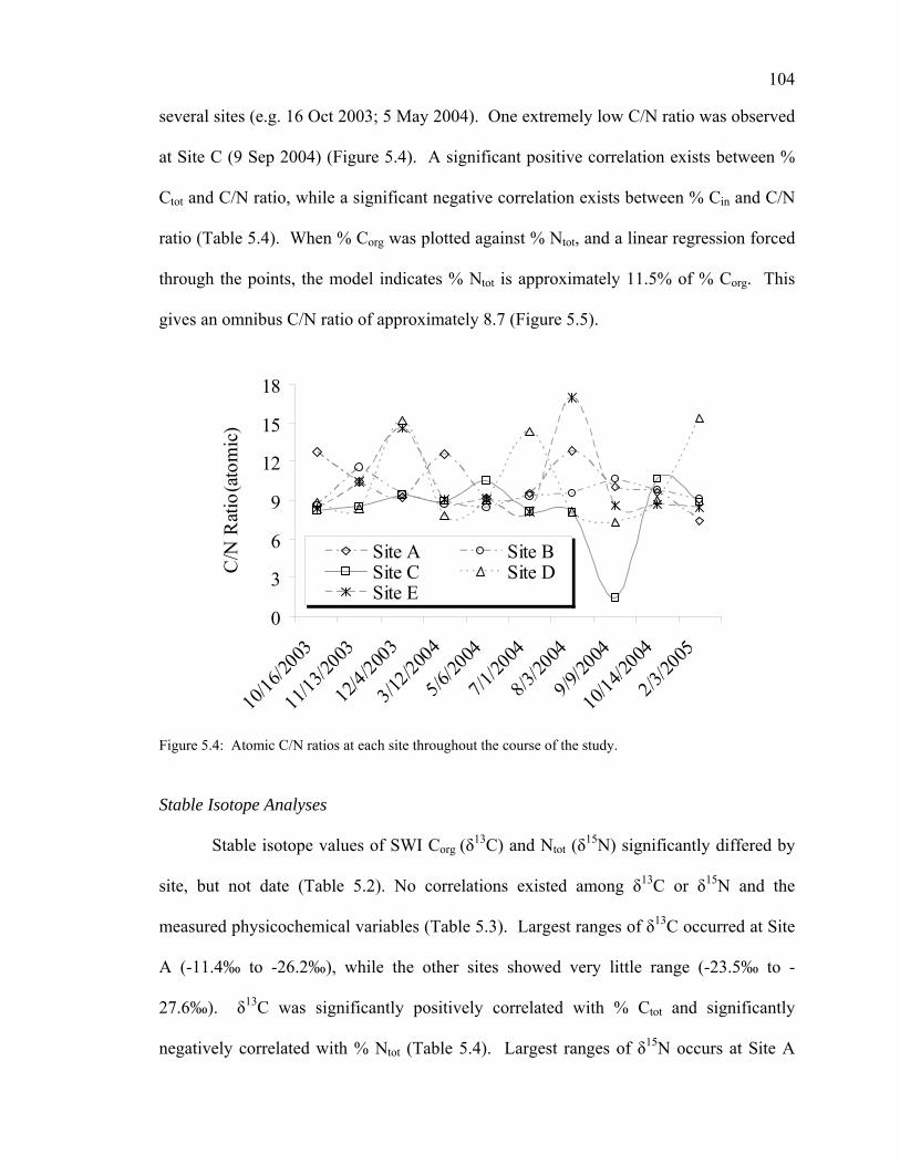
104
several sites (e.g. 16 Oct 2003; 5 May 2004). One extremely low C/N ratio was observed
at Site C (9 Sep 2004) (Figure 5.4). A significant positive correlation exists between %
Ctot and C/N ratio, while a significant negative correlation exists between % Cin and C/N
ratio (Table 5.4). When % Corg was plotted against % Ntot, and a linear regression forced
through the points, the model indicates % Ntot is approximately 11.5% of % Corg. This
gives an omnibus C/N ratio of approximately 8.7 (Figure 5.5).
0
3
6
9
12
15
18
10/16
/2003
11/13/2
003
12/4/
2003
3/12/20
04
5/6/20
04
7/1/20
04
8/3/20
04
9/9/20
04
10/14/2
004
2/3/20
05
C/N
Rat
io (a
tom
ic)
Site A Site BSite C Site DSite E
Figure 5.4: Atomic C/N ratios at each site throughout the course of the study. Stable Isotope Analyses
Stable isotope values of SWI Corg (δ13C) and Ntot (δ15N) significantly differed by
site, but not date (Table 5.2). No correlations existed among δ13C or δ15N and the
measured physicochemical variables (Table 5.3). Largest ranges of δ13C occurred at Site
A (-11.4‰ to -26.2‰), while the other sites showed very little range (-23.5‰ to -
27.6‰). δ13C was significantly positively correlated with % Ctot and significantly
negatively correlated with % Ntot (Table 5.4). Largest ranges of δ15N occurs at Site A
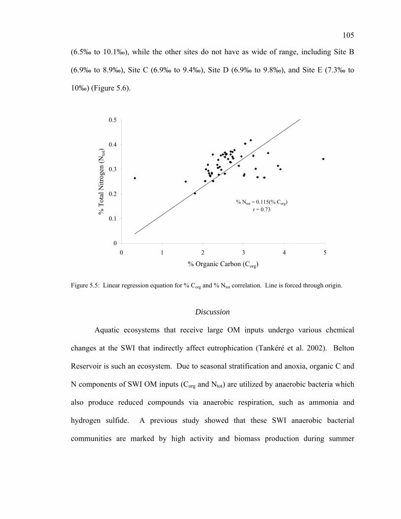
105
(6.5‰ to 10.1‰), while the other sites do not have as wide of range, including Site B
(6.9‰ to 8.9‰), Site C (6.9‰ to 9.4‰), Site D (6.9‰ to 9.8‰), and Site E (7.3‰ to
10‰) (Figure 5.6).
% Ntot = 0.115(% Corg)r = 0.73
0
0.1
0.2
0.3
0.4
0.5
0 1 2 3 4 5
% Organic Carbon (Corg)
% T
otal
Nitr
ogen
(Nto
t)
Figure 5.5: Linear regression equation for % Corg and % Ntot correlation. Line is forced through origin.
Discussion
Aquatic ecosystems that receive large OM inputs undergo various chemical
changes at the SWI that indirectly affect eutrophication (Tankéré et al. 2002). Belton
Reservoir is such an ecosystem. Due to seasonal stratification and anoxia, organic C and
N components of SWI OM inputs (Corg and Ntot) are utilized by anaerobic bacteria which
also produce reduced compounds via anaerobic respiration, such as ammonia and
hydrogen sulfide. A previous study showed that these SWI anaerobic bacterial
communities are marked by high activity and biomass production during summer

106
stratification (see Chapter 2). The study contradicted conventional wisdom that
advocates greater bacterial activities and biomass production (requiring Corg and Ntot)
-28
-25
-22
-19
-16
-13
-10
δ13C
org
(‰)
0
2
4
6
8
10
12
10/16/20
03
11/13/2003
12/4/2003
3/12/200
4
5/6/2004
7/1/2004
8/3/200
4
9/9/2004
10/14/2004
2/3/2005
δ15Ntot (‰
)
-28
-25
-22
-19
-16
-13
-10
δ13C
org
(‰)
0
2
4
6
8
10
12
10/16/20
03
11/13/2003
12/4/2003
3/12/200
4
5/6/2004
7/1/2004
8/3/200
4
9/9/2004
10/14/2004
2/3/2005
δ15Ntot (‰
)
-28
-25
-22
-19
-16
-13
-10
δ13C
org
(‰)
0
2
4
6
8
10
12
10/16/20
03
11/13/2003
12/4/2003
3/12/2004
5/6/2004
7/1/2004
8/3/2004
9/9/2004
10/14/2004
2/3/2005
δ15Ntot (‰
)
-28
-25
-22
-19
-16
-13
-10δ1
3Cor
g (‰
)
0
2
4
6
8
10
12
10/16/20
03
11/13/2003
12/4/2003
3/12/2004
5/6/2004
7/1/2004
8/3/2004
9/9/2004
10/14/2004
2/3/2005
δ15Ntot (‰
)
-28
-25
-22
-19
-16
-13
-10
δ13C
org
(‰)
0
2
4
6
8
10
12
10/16/20
03
11/13/2003
12/4/2003
3/12/2004
5/6/2004
7/1/2004
8/3/2004
9/9/2004
10/14/2004
2/3/2005
δ15Ntot (‰
)
Figure 5.6: Stable isotope values for δ13C (▲) and δ15N (♦) at each site over the course of the study.
Site A Site B
Site C
Site E
Site D
107
when oxygen, with its large free energy potential, is the preferred electron acceptor
(Wirtz 2003). The goal of this study was to propose various ways that these SWI
bacterial communities quantitatively and qualitatively affect SWI OM due to seasonal
stratification and mixing events on a spatial and temporal basis.
Bulk Organic Matter Sources and Sinks
The significant negative correlation between OM concentration and dissolved
oxygen suggests higher OM degradation under higher dissolved oxygen concentration.
This seemingly contradicts the study that concluded higher SWI bacterial activity, thus
degradation of OM, occurs under anoxic conditions (see Chapter 2). However, a
substantial portion of SWI bacterial activity under anoxia also includes chemolithotrophic
metabolism and fermentative metabolism of small dissolved organic compounds that may
go undetected in bulk OM measurements.
Another possibility accounting for the inverse relationship between dissolved
oxygen and OM concentration is increased SWI OM deposition during summer
stratification due to binding of OM to dissolved calcite (CaCO3) under anoxic conditions,
which increases the OM sinking to the SWI (Hodell and Schelske 1998). CaCO3
commonly precipitates from epilimnetic waters in the summer, and exists in high
concentrations in Belton Reservoir (Dr. Steve Dworkin, Baylor University, personal
communication).
However, SWI OM concentrations were not significantly different among
seasons. This in and of itself does not imply that SWI OM inputs were quantitatively
similar among seasons, but that net burial of OM to the sediments is relatively equal,
regardless of oxic or anoxic conditions. For example, rates of OM degradation may be
108
dependent not only on rates of aerobic or anaerobic bacterial mineralization, but also the
quality of organic matter present. Inputs of simple carbohydrates, lipids, and proteins are
readily utilized by both aerobic and anaerobic bacteria (Lehmann et al. 2002). Thus it is
possible that bacteria completely utilize all labile OM under oxic and anoxic conditions,
but all recalcitrant OM, which comprises the majority of OM, exhibits little difference in
quantity among seasons and is thus permanently deposited (Jonsson et al. 2001).
Carbon Dynamics
Differences in SWI Ctot occurred on a spatial, but not seasonal scale. Corg did not
significantly differ among site, which was not surprising considering that OM, of which
Corg is a component, did not differ spatially. Instead, the spatial Ctot differences were
attributed to high concentrations of inorganic carbon (Cin) at Sites A, B, and C.
Limestone cliffs (composed of CaCO3) surrounding Belton Reservoir possibly serves as
an allochthonous source of Cin due to weathering and runoff during rain events. Sites D
and E had low Cin, and were located further away from the cliffs than Sites A, B, and C,
possibly accounting for the Cin differences.
However, autochthonous processes may also account for higher Cin at Sites A, B,
and C. Algal photosynthesis in the epilimnion during the summer consumes CO2, which
increases pH and produces CaCO3 (Horne and Goldman 1994). If high pH is maintained
at the SWI (such as Site A due to only weak stratification), CaCO3 directly precipitates to
the sediment surface. Under prolonged anoxic conditions (Sites D and E), pH and redox
potential are low, thus CaCO3 dissolves and is only deposited if bound to organic matter
from the epilimnion (Hodell and Schelske 1998). At intermediate pH and redox
potentials, such as Sites B and C during stratification, redox potential is within a range
109
that results in ferric iron reduction. Iron reduction, coupled with pH that is low enough to
dissolve CaCO3, produces siderite (FeCO3) that precipitates to the SWI. However this
process does not completely remove all dissolved CaCO3, thus the amount of Cin at the
SWI will not be as large as those that have direct deposition of CaCO3 (Dean 1999).
Sites A through E follow this gradient, as observed in Figure 5.2.
Nitrogen Dynamics
Significant differences in % Ntot among dates suggest that SWI OM sources
and/or use of nitrogen-containing OM by SWI bacteria vary by season. Referring to
Figure 5.3, lowest % Ntot occurred during winter mixing (4 Dec 2003; 3 Feb 2005; and
with the exception of Site 3, 12 Mar 2004). This is supported by the negative correlation
between % Ntot with dissolved oxygen and pH. This contradicts studies that suggest wind
and rain events during winter mixing often increases inputs of allochthonous OM in
reservoirs, which contain nitrogen-rich compounds (Thornton and McManus 1994).
Further, differences in % Ntot among sites are due to lower values at Sites A and B,
possibly due to higher cellulose-rich allochthonous inputs (i.e. lower C/N ratio) at these
sites due to closer proximity to the shoreline.
During winter mixing in Belton Reservoir, SWI bacteria preferred utilization of
carbohydrates which lack nitrogen over amino acids which contain nitrogen. Amino
acids were preferred by SWI bacteria during stratification (see Chapter 4). When
interpreted in context of this study, non-nitrogen containing compounds are preferred by
SWI bacteria when SWI Ntot is low. Thus it is possible that during winter mixing SWI
bacteria are selected for taxa that obtain a sufficient amount of nitrogen under low Ntot.
Higher Ntot present during stratification may select for bacteria that require higher
110
concentrations of nitrogen, thus those that readily use amino acids. An alternative
explanation is that high amino acid utilization during stratification is due to bacterial
nitrogen limitation, suggesting that the nitrogen present during stratification, while
abundant, may be unusable by the anaerobic bacteria (Hollibaugh and Azam 1983).
C/N Ratios
C/N ratios are used as a proxy to determine OM that originates from
autochthonous as opposed to allochthonous sources. These ratios are often used in
conjunction with stable isotope measurements of C and N. Corg/Ntot ratios between 4 and
10 generally indicate OM present from sinking phytoplankton, while ratios greater than
20 indicate OM from cellulose-rich allochthonous sources (i.e. C3 land plants) (Meyers
and Teranes 2001).
With the exception of one anomalous sample, all C/N ratios range from 7.3 to
16.9, median 9.1. Thus these SWI OM samples are close to the predicted range of OM
from sinking autochthonous production. This median ratio falls between the sediment
C/N ratios for Lake Ontario (median = 8) and Lake Baikal (median = 11) (Hodell and
Schelske 1998; Qiu et al. 1993).
The positive correlations between % Ntot with % Ctot and % Corg explain the lack
of significant difference of C/N ratios (% Corg / % Ntot) among site or date. Had
differences in C/N ratios existed, the positive correlation between % Ctot and % Ntot
would not be observed. A linear model of best-fit, forced through the origin predicts an
omnibus C/N ratio of 8.7, only 4.3% less than the actual median value.
Conceivably, seasonal differences in bacterial activity coupled with selective
preferences in C-rich or N-rich compounds, could affect the measured C/N ratio. Thus

111
the ratio would not only be a function of allochthonous or autochthonous inputs, but also
of bacterial utilization of OM. However, bacterial utilization of C and N is usually not
significant enough to affect interpretation of C/N ratios being from algae or land plants
(Meyers and Teranes 2001).
Stable Isotope Dynamics
Ratios of 13C to 12C (δ13Corg) and 15N to 14N (δ15Ntot) in lake sediment OM are
used to assess OM sources, C and N utilization by various organisms, and reconstruction
of past productivity. This is based on evidence that algae preferentially uptake 12C over
13C, thus δ13C values of sediment from autochthonous production are lower (i.e.
isotopically lighter) than δ13C values of sediment from terrestrial OM sources, which has
a preference for 13C uptake. Algae also preferentially uptake 15N over 14N because of
high 15N values in nitrate, the preferred algal nitrogen source. Terrestrial plants are
higher in 14N because their preferential nitrogen uptake is atmospheric which does not
contain 15N. Thus δ15N values are higher from sediment whose sources are
autochthonous (Meyers and Teranes 2001; Hoefs 2004).
Spatial differences in stable isotope values for δ13C and δ15N were attributed to
significantly different isotope signatures at Site A as opposed to the other sites. The
median δ13C signature at Site A was -17.2 ‰. This δ13C signature at Site A corresponds
to the signature commonly seen in C4 vascular plants, unlike the δ13C signatures at the
other sites that correspond to algae. Unlike C/N ratios, this stable isotope signature
clearly shows the difference in Site A OM sources. Thus, Site A SWI OM is influenced
by allochthonous inputs unlike the other sites that are clearly dominated by
autochthonous production.
112
While the δ15N signature was significantly lighter at Site A than other sites, its
median value was 7.83 ‰, still in the range commonly seen in lake sediments, which
normally ranges from 0 ‰ to 10 ‰ (Hoefs 2004). The lighter signature was possibly due
to input of allochthonous OM which has a typical δ15N signature of -1 ‰ to 3 ‰, which
dilutes the overall δ15N signature. Because sites B through E exhibit strong seasonal
anoxic patterns, the range of δ15N signatures observed at the SWI of these sites is
possibly a function of both OM source and fate. The source corresponds to that of
sinking algae and phytodetritus, while fate (i.e. transformation) corresponds to
denitrification from bacteria under anoxic conditions (Meyers and Teranes 2001).
Conclusions
SWI bacterial metabolism is often much greater than bacterial metabolism in the
overlying water column, therefore SWI bacterial degradation and mineralization of OM
substantially affects reservoir carbon and nitrogen cycling. In a stratified, eutrophic
reservoir with highly variable SWI bacterial activities, OM quantity was not only a
function of the bacteria, but also of the depth and surrounding landscape of the reservoir.
Allochthonous processes play an important role in OM burial at shallow sites, more so
than at deeper sites in which OM burial is completely of autochthonous origin. Shallow
sites that are near shore also only weakly undergo stratification, thus pH, redox, and
mixing activities affected Cin, C/N ratios, δ13C, and δ15N. This demonstrates that
quantitatively important SWI OM dynamics are a function of physical and chemical, as
well as biological, processes.
113
Acknowledgments
This research was made possible by funding from the Jack G. and Norma Jean
Folmar Research Grant and Bob Gardner Memorial Grant, both through Baylor
University. We thank Dr. Steve Dworkin (Baylor University) for use of the CHN
analyzer and manuscript criticism. We also thank Glenn Piercey and Thomas Millican
with the University of Arkansas Stable Isotope Laboratory for stable isotope analysis.
Valuable field assistance was provided by David Clubbs. Field assistance and
manuscript input was provided by Christopher Filstrup.
114
CHAPTER SIX
Presence and Diversity of Total and Sulfate-Reducing Bacteria at the Sediment-Water Interface of a Stratified, Eutrophic Reservoir
Introduction
Sediment-water interfaces (SWIs) in thermally stratified eutrophic reservoirs are
seasonally blanketed by anoxic hypolimnia due to water column temperature gradients
and bacterial consumption of hypolimnetic dissolved oxygen. Oxygen depletion selects
for hypolimnetic bacterial assemblages that anaerobically oxidize various organic carbon
substrates (Tammert et al. 2005). In anaerobic respiration, electron acceptors (e.g.
nitrate, ferric iron, sulfate) are reduced in order of their decreasing free energy and often
form a vertical redox potential gradient (Nealson and Stahl 1997). These redox processes
also occur among the bacterial assemblages at the SWI on a much smaller, often
micrometer, scale. The depth of the SWI redox gradient partially depends on the mixing
conditions overlying water. Further, SWIs contain bacteria at abundances higher than the
water column, and these bacteria are highly active (see Chapter Two). Various studies
have addressed many SWI bacterial processes, however an adequate measure of SWI
bacterial community similarity and diversity, specifically on a seasonal basis in stratified
reservoirs is lacking.
Historically, bacterial taxonomic and diversity studies have lacked an applied
aspect, relegating such studies to lesser importance in understanding reservoir ecosystem
dynamics. Much of this relies on the fact that bacterial diversity and function
measurements historically have suffered from methodological limitations. Yet,
115
understanding bacterial diversity in freshwater ecosystems has become increasingly
important in understanding aspects of eutrophication and in development of theoretical
models that predict reservoir trophic dynamics (Torsvik et al. 2002).
Traditional measures of bacterial diversity in environmental matrices involved
selective culturing methods. However, culturing drastically underestimates true bacterial
diversity because the vast majority of naturally occurring bacteria are unculturable (Kirk
et al. 1998). Molecular biology techniques have reduced these biases and limitations by
preserving the original sample bacterial diversity. Diversity includes richness which is
the number of different operational taxonomic units (OTUs) (also known as taxon or
species), and evenness which is the amount of each OTU relative to the entire community
(Hewson and Fuhrman 2004). Molecular fingerprinting methods that have been utilized
to measure bacterial diversity included DNA reassociation kinetics, restriction and
terminal-restriction fragment length polymorphisms (RFLPs and t-RFLPs), denaturing
gradient gel electrophoresis (DGGE), and automated intergenic ribosomal spacer analysis
(ARISA). Each of these methods provide various degrees of resolution, therefore
multiple methods are often used to profile bacterial communities (MacGregor 1999). We
utilized both DGGE and ARISA to measure seasonal diversity and similarity of SWI
bacterial communities in a seasonally stratified reservoir. ARISA was used to profile the
entire bacterial community, while DGGE was used to profile the richness of sulfate
reducing bacteria (SRB).
The microbial loop concept redefined traditional understanding of aquatic food
chain dynamics (Pomeroy 1974; Sherr and Sherr 1988). Novel to the microbial loop was
the role of heterotrophic bacteria in organic matter cycling. SWIs are quantitatively
116
important as organic matter sinks and sources in lakes, mediated by SWI bacterial
communities. However, studies of SWI bacterial dynamics lags behind those of open
water. This investigation measured total SWI bacterial community diversity and
similarity on a seasonal basis and related these measurements to seasonal reservoir
mixing dynamics. Because of the importance of sulfur cycling in freshwater ecosystems,
SRB diversity was also measured. The SWI of the study site, Belton Reservoir, has a
highly active bacterial community with various populations utilizing a wide variety of
organic carbon sources (see Chapters 2 and 4). However, until now, the relative diversity
of this SWI bacterial community has remained unknown.
Materials and Methods
Study Location
The investigation was conducted on the SWI of Belton Reservoir, a warm,
monomictic reservoir in central Texas. Belton Reservoir is eutrophic and undergoes
lacustrine zone thermal stratification during late spring and summer, developing an
anoxic hypolimnion (Christian et al. 2002; Figure 1.1). The lacustrine zone exhibits a
steep depth gradient along its longitudinal axis. The anoxic hypolimnion blanketing this
gradient varies spatially and temporally in depth and duration. Five SWI sites along a
linear transect of this gradient were chosen for sampling, with each site of increasing
depth (Figure 1.2, Table 4.3).
Physicochemical characteristics of the SWI [e.g. temperature (ºC), dissolved
oxygen (mg l-1), redox potential (mV), pH] were measured with a YSI 600QS Sonde,
lowered to the sediment surface and allowed to stabilize (Table 5.1).
117
Sample Collection and Processing
SWI samples were collected from the five sampling sites over multiple seasons,
corresponding to the various seasonal mixing and stratification conditions of the reservoir
(Table 5.1). Sediment samples were collected from the SWI using a 15 cm x 15 cm
Ekman dredge. Three samples were collected at each site. Upon retrieval, excess water
was carefully siphoned from the sample surface and liquid nitrogen was poured slowly
into the corner of the dredge so that disruption of the SWI matrix was minimized. The
frozen sediment block was removed from the dredge, wrapped in aluminum foil, sealed
in plastic, and held on dry ice. Blocks were returned to the laboratory and held at -80ºC
until processing.
For each sediment block, the upper 10 mm of sediment was shaved from the top,
placed into a 50 ml plastic centrifuge tube and homogenized. This layer was defined as
the SWI, and was determined based on the average depth of the sediment that achieved
the lowest redox potential as measured on aerobically and anaerobically incubated
microcosm samples using a Unisense© RD-10 redox microelectrode (see Chapter Five).
From each sample, approximately 1 g of the homogenized sediment was
preserved in 9 ml of formalin and refrigerated at 4°C for later measurement of bacterial
abundance. Another 1 g of sediment was added to a bead solution tube (MoBio) for
DNA extraction. The remaining sediment was added to a pre-weighed crucible for
organic matter analysis (see Chapter Five).
Bacterial Abundance Measurements
To separate bacteria from sediments, a combination of chemical and physical
dispersion was used. Formalin-preserved sediment samples were vortexed briefly,

118
followed by addition of 50 µl of Tween 80. The samples were shaken on a rotary shaker
at 500 rpm for 20 minutes, followed by sonication at 50 W for 30 s. One-hundred µl of
the slurry was added to 900 µl of bacteria-free water (0.2-µm filtered) in a 2 ml
microcentrifuge tube and centrifuged at 15,000 x g for 2 minutes. The supernatant was
transferred to a clean 2 ml microcentrifuge tube. The precipitate was resuspended in 1 ml
of bacteria-free water and centrifuged again at 15,000 x g for 2 minutes. The supernatant
was transferred to the centrifuge tube containing the previous supernatant. Random
samples were chosen for a third resuspension/centrifugation step, but the supernatant
from this step did not contain a significant number of bacteria (< 106 bacteria ml-1).
One-hundred µl of supernatant was added to 900 µl of bacteria-free water and
stained with DAPI fluorochrome (5 µg ml-1 final concentration) for 3 minutes. The
stained sample was filtered onto a 0.2-µm Nuclepore blackened polycarbonate filter and
viewed under UV light at 1500 x magnification (Porter and Feig 1980). For any
remaining particle-attached bacteria, a 2 x correction factor was applied (Lind and
Dávalos-Lind 1991). Bacterial concentration was converted to total cells per gram dry
weight of sediment (bacteria gdw-1) (Ellery and Schleyer 1984; Ramsay 1984; dos Santos
Furtado and Casper 2000).
DNA Extraction
A MoBio UltraClean™ Soil DNA kit was used to extract and purify total
genomic DNA from sediment samples. Approximately 1 g of sediment was used per
extraction, with the exact amount weighed into a bead solution tube. Two separate
extractions were performed on separate subsamples of a sample.
119
Resulting DNA was quantified and checked for purity using a GeneQuant™ Pro
DNA calculator. If both subsamples were of sufficient purity (A260/A280 = 1.8 - 2.0), then
they were combined and quantified. If a subsample was not of sufficient purity, then it
was discarded. DNA concentration of all samples were recorded as ng µl-1 and
normalized per gram dry weight of sediment (see Chapter Five).
ARISA Analysis
The primer set ITSF and ITSReub (Integrated DNA, Coralville, Iowa)
complementary to portions of the 16S and 23S rRNA genes (16s rDNA) of eubacteria
was used in a polymerase chain reaction (PCR) to amplify bacterial DNA corresponding
to the intergenic spacer region between 16S and 23S rDNA (Cardinale et al. 2004) (Table
6.1). The 5’ end of the ITSF primer was labeled with WellRED D4 phosphoramidite dye
to allow fluorometric analysis of the PCR amplified fragments using an automated
fragment analyzer.
Table 6.1: Primer sequences used in this study, their common name, and gene targeted.
Target Gene Primer Name Sequence (5' - 3') Reference
16S rRNA ITSF GTCGTAACAAGGTAGCCGTA Cardinale et al. 199823S rRNA ITSFReub GCCAAGGCATCCACC Cardinale et al. 1998dsrB DSRp2060Fa CAACATCGTYCAYACCCAGGG Geets et al. 2006dsrB DSR4R GTGTAGCAGTTACCGCA Wagner et al. 1998
GC Clampb CGCCCGCCGCGCCCCGCGCC- Schäfer and Muyzer 2001CGTCCCGCCGCCCCCGCCCG
a where Y = C/Tb GC clamp is attached to 5' end of DSRp2060F primer
Two µl of sediment-extracted DNA was added to a reaction mixture containing
(final concentration) 1x PCR buffer, 2.5 mM MgCl2, 200 µM each dNTP, 400 ng µl-1
120
bovine serum albumin, 1.25 U of Taq polymerase, and 15 pmol of each primer in a final
volume of 50 µl. PCR conditions were a 94ºC initial denaturation for 3 min, followed by
35 cycles of a 1 min denaturation at 94ºC, 1 min annealing at 53ºC, and 2 min elongation
at 72ºC, followed by a final extension at 72ºC for 5 min. All PCR products were
electrophoresed on a 1% horizontal agarose gel at 120 V for 90 min to insure that proper
amplified products (50 bp – 1200 bp) were obtained.
A mixture containing 3 µl of the PCR product and 1 µl of a Bioventures size
standard (50-1000 bp in 20 and/or 50 bp increments) was added to 36 µl of deionized
formamide and injected into a Beckman Coulter™ CEQ 8000 Genetic Analysis System
using a modified FRAG-4 separation method with a 50ºC capillary temperature and a 5
kV separation voltage for 150 min.
Resulting separation profiles (electropherograms) were analyzed with the
Beckman Coulter Fragment Analysis Package v.8.0. A quartic analysis model was used
with a slope threshold parameter of 5 and PA version 1 dye mobility calibration.
Electropherograms consisted of a series of peaks. Because each bacterial taxon
has a specific size and composition of their intergenic space, each peak represented an
individual operational taxonomic unit (OTU). The area underneath each peak was
divided by the total area under the entire electropherogram to calculate relative
abundance of each OTU (Figure 6.1). Relative abundance and richness (i.e. number of
peaks in an electropherogram) were used to calculate the Shannon-Weiner diversity index
(H) and Shannon-Weiner evenness (EH). Higher H indicates more diverse communities
(i.e. higher number of species and comparative relative abundance), while EH values
indicate the proportion of individuals among the species, indicating if there are dominant

121
populations (i.e. EH values closer to 1 indicate complete evenness) (Begon et al. 1996;
Atlas and Bartha 1998).
Figure 6.1: Example of an electropherogram. From Site D, 13-Nov-03. DGGE Analysis of Sulfate Reducing Bacteria
The primer set DSRp2060F and DSR4R (Integrated DNA, Coralville, Iowa) that
amplifies a 350 bp segment of the dsrB gene in sulfate reducing bacteria (SRB) was used
(Geets et al. 2006) (Table 6.1). A 40 bp GC-clamp was added to the 5’ end of the
forward primer to allow products to run on denaturing gradient gels (Muyzer et al. 1993).
The PCR amplification consisted of a reaction mixture of (final concentration) 1 x
PCR buffer, 1.5 mM MgCl2, 200 µM each dNTP, 400 ng µl-1 bovine serum albumin, 2.5
U of Taq polymerase 50 pmol of each primer, and 2 µl of sediment-extracted DNA in a
total volume of 100 µl. PCR conditions were an initial denaturation for 4 min at 94ºC,
followed by 35 cycles of a 1 min denaturation at 94ºC, 1 min annealing at 55ºC, and 1
min elongation at 72ºC, followed by a final 10 min extension at 72ºC (Janse et al. 2004).
The PCR products were electrophoresed on a 1% horizontal agarose gel at 120 V for 90
122
min to insure that proper amplified products were obtained. All amplified products were
the same length (350 bp), but of various sequences.
10 µl of amplified PCR product was loaded onto a 1 mm-thick 8 % (w/v)
polyacrylamide gel with a 40% - 60% gradient of urea/formamide denaturant. The
vertical gels were electrophoresed at 75 V for 16 h at 60ºC in 1 x TAE using a dual-
cassette DGGE System (Model 2401, CBS Scientific, California). After electrophoresis,
gels were stained with SYBR® Gold Nucleic Acid Gel Stain (Molecular Probes, Oregon)
diluted 1:10,000 in 1 x TAE buffer for 45 min followed by a 15 min rinse in deionized
water. Gels were photographed under UV trans-illumination (540 nm) with an Omega
Ultra LumTM gel imaging system. Further gel imaging and processing was conducted
with Omega UltraQuantTM imaging and analysis software v 6.0 and Adobe® Photoshop®
v 9.0.
Statistical Analyses
Descriptive and univariate statistics (e.g. linear regression, one-way ANOVA)
were performed with JMP v 5.0 (SAS Institute, California) and Microsoft Excel XP. A
significance level of α = 0.05 was assumed. Microsoft Excel was also used for graphical
analyses.
For ARISA analyses, a spreadsheet was generated containing individual samples
(columns) and base pair sizes from 50 to 1200 (rows). The presence or absence of a
specific base pair size for each sample was recorded as a 1 or 0, respectively. From this
binary matrix, a Jaccard similarity index was generated, using PopTools v 2.7.5 (CSIRO,
Australia). Using PHYLIP v 3.65 phylogeny inference package, the Neighbor-Joining
method of clustering analysis was performed on the Jaccard matrix to generate a
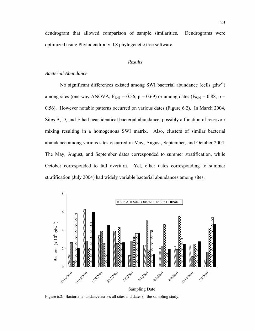
123
dendrogram that allowed comparison of sample similarities. Dendrograms were
optimized using Phylodendron v 0.8 phylogenetic tree software.
Results
Bacterial Abundance
No significant differences existed among SWI bacterial abundance (cells gdw-1)
among sites (one-way ANOVA, F4,45 = 0.56, p = 0.69) or among dates (F9,40 = 0.88, p =
0.56). However notable patterns occurred on various dates (Figure 6.2). In March 2004,
Sites B, D, and E had near-identical bacterial abundance, possibly a function of reservoir
mixing resulting in a homogenous SWI matrix. Also, clusters of similar bacterial
abundance among various sites occurred in May, August, September, and October 2004.
The May, August, and September dates corresponded to summer stratification, while
October corresponded to fall overturn. Yet, other dates corresponding to summer
stratification (July 2004) had widely variable bacterial abundances among sites.
0
2
4
6
8
10/16
/2003
11/13
/2003
12/4/
2003
3/12/2
004
5/6/20
04
7/1/20
04
8/3/20
04
9/9/20
04
10/14
/2004
2/3/20
05
Sampling Date
Bac
teria
(x 1
08 gdw
-1)
Site A Site B Site C Site D Site E
Figure 6.2: Bacterial abundance across all sites and dates of the sampling study.
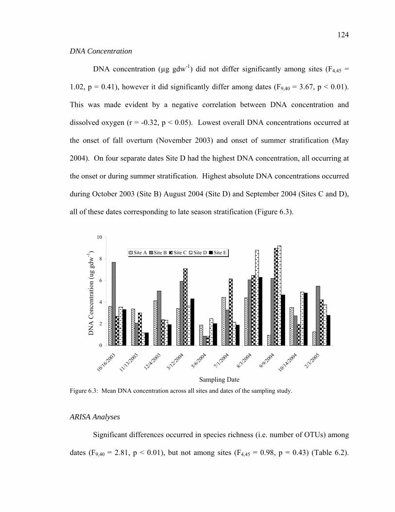
124
DNA Concentration
DNA concentration (µg gdw-1) did not differ significantly among sites (F4,45 =
1.02, p = 0.41), however it did significantly differ among dates (F9,40 = 3.67, p < 0.01).
This was made evident by a negative correlation between DNA concentration and
dissolved oxygen (r = -0.32, p < 0.05). Lowest overall DNA concentrations occurred at
the onset of fall overturn (November 2003) and onset of summer stratification (May
2004). On four separate dates Site D had the highest DNA concentration, all occurring at
the onset or during summer stratification. Highest absolute DNA concentrations occurred
during October 2003 (Site B) August 2004 (Site D) and September 2004 (Sites C and D),
all of these dates corresponding to late season stratification (Figure 6.3).
0
2
4
6
8
10
10/16
/2003
11/13
/2003
12/4/
2003
3/12/2
004
5/6/20
04
7/1/20
04
8/3/20
04
9/9/20
04
10/14
/2004
2/3/20
05
Sampling Date
DN
A C
once
ntra
tion
(ug
gdw
-1) Site A Site B Site C Site D Site E
Figure 6.3: Mean DNA concentration across all sites and dates of the sampling study. ARISA Analyses Significant differences occurred in species richness (i.e. number of OTUs) among
dates (F9,40 = 2.81, p < 0.01), but not among sites (F4,45 = 0.98, p = 0.43) (Table 6.2).
125
Highest richness was not correlated with any specific season, as significantly higher
richness was present in May 2004 (onset of stratification), July 2004 (summer
stratification), October 2004 (autumnal overturn), and February 2005 samples (winter
mixing). Lower richness was present in March 2004 (winter mixing), as well as August
and September 2004 samples which exhibited total anoxia and lowest redox potential.
No significant difference existed for Shannon-Weiner Diversity (H) by date (F9,40
= 1.41, p = 0.22) or by site (F4,45 = 0.78 p = 0.54) (Table 6.2). In addition, no significant
difference existed for Shannon-Weiner Evenness (EH) by date (F9,40 = 0.77, p = 0.64) or
by site (F4,45 = 0.35, p = 0.85) (Table 6.2).
Figure 6.4 relates the similarity among the SWI bacterial communities. Samples
during stratification and anoxia were highly similar. For example, in July 2004 Sites C,
D, and E were highly similar; during August 2004 all sites were highly similar; and in
September 2004 all sites were highly similar with the exception of Site A. In October
2003, Sites B and E were similar as were Sites C and D. The high similarities correspond
directly to anoxia or hypoxia (< 1 mg l-1). The dissimilar sites all have > 1 mg l-1
dissolved oxygen.
Similarities among sites also occurred during winter mixing, but were not as
pronounced and sequential as during stratification. In December 2003, Sites A, B, and
D were similar; in March 2004 Sites A, B, and C were similar; in February 2005 sites had
high similarity with the exception of Site D.
During overturn during October 2004, high similarity occurred; however during
overturn in November 2003, with the exception of Sites A and E, samples were highly
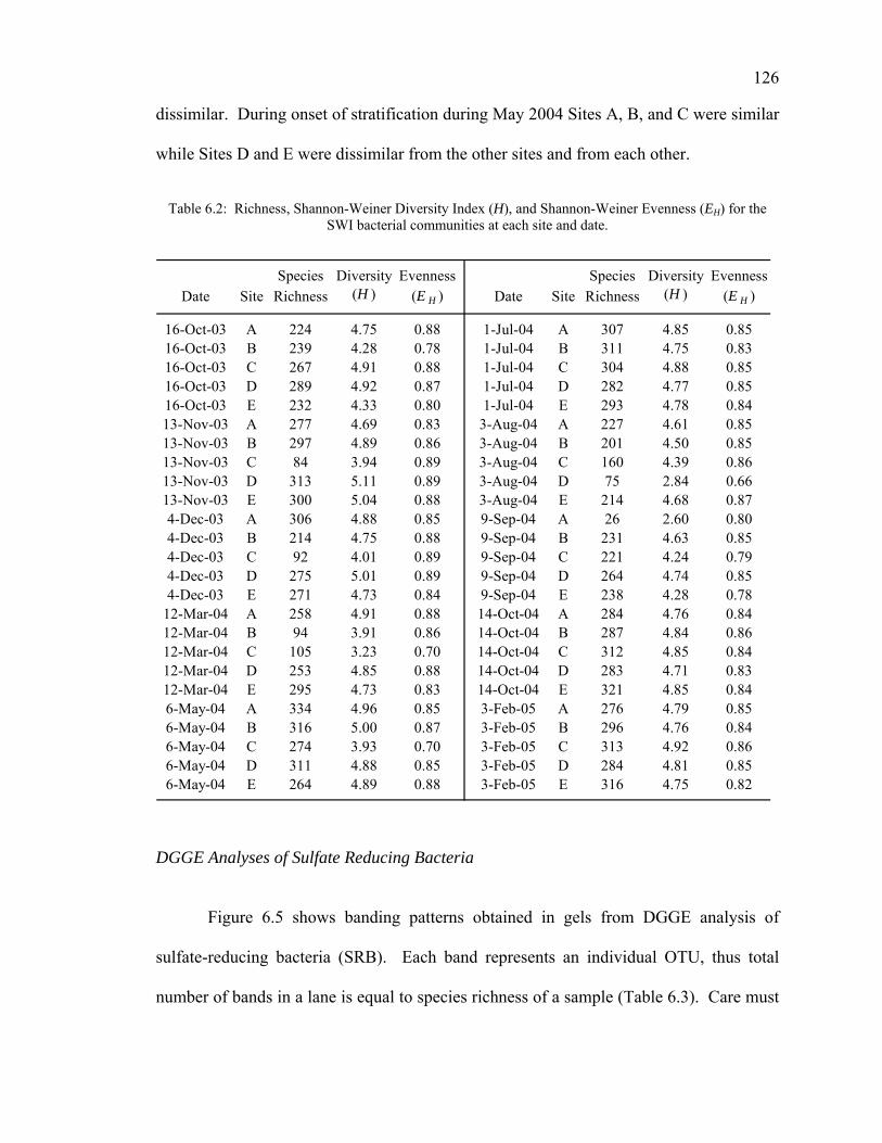
126
dissimilar. During onset of stratification during May 2004 Sites A, B, and C were similar
while Sites D and E were dissimilar from the other sites and from each other.
Table 6.2: Richness, Shannon-Weiner Diversity Index (H), and Shannon-Weiner Evenness (EH) for the
SWI bacterial communities at each site and date.
Species Diversity Evenness Species Diversity EvennessDate Site Richness (H ) (E H ) Date Site Richness (H ) (E H )
16-Oct-03 A 224 4.75 0.88 1-Jul-04 A 307 4.85 0.8516-Oct-03 B 239 4.28 0.78 1-Jul-04 B 311 4.75 0.8316-Oct-03 C 267 4.91 0.88 1-Jul-04 C 304 4.88 0.8516-Oct-03 D 289 4.92 0.87 1-Jul-04 D 282 4.77 0.8516-Oct-03 E 232 4.33 0.80 1-Jul-04 E 293 4.78 0.8413-Nov-03 A 277 4.69 0.83 3-Aug-04 A 227 4.61 0.8513-Nov-03 B 297 4.89 0.86 3-Aug-04 B 201 4.50 0.8513-Nov-03 C 84 3.94 0.89 3-Aug-04 C 160 4.39 0.8613-Nov-03 D 313 5.11 0.89 3-Aug-04 D 75 2.84 0.6613-Nov-03 E 300 5.04 0.88 3-Aug-04 E 214 4.68 0.874-Dec-03 A 306 4.88 0.85 9-Sep-04 A 26 2.60 0.804-Dec-03 B 214 4.75 0.88 9-Sep-04 B 231 4.63 0.854-Dec-03 C 92 4.01 0.89 9-Sep-04 C 221 4.24 0.794-Dec-03 D 275 5.01 0.89 9-Sep-04 D 264 4.74 0.854-Dec-03 E 271 4.73 0.84 9-Sep-04 E 238 4.28 0.78
12-Mar-04 A 258 4.91 0.88 14-Oct-04 A 284 4.76 0.8412-Mar-04 B 94 3.91 0.86 14-Oct-04 B 287 4.84 0.8612-Mar-04 C 105 3.23 0.70 14-Oct-04 C 312 4.85 0.8412-Mar-04 D 253 4.85 0.88 14-Oct-04 D 283 4.71 0.8312-Mar-04 E 295 4.73 0.83 14-Oct-04 E 321 4.85 0.846-May-04 A 334 4.96 0.85 3-Feb-05 A 276 4.79 0.856-May-04 B 316 5.00 0.87 3-Feb-05 B 296 4.76 0.846-May-04 C 274 3.93 0.70 3-Feb-05 C 313 4.92 0.866-May-04 D 311 4.88 0.85 3-Feb-05 D 284 4.81 0.856-May-04 E 264 4.89 0.88 3-Feb-05 E 316 4.75 0.82
DGGE Analyses of Sulfate Reducing Bacteria
Figure 6.5 shows banding patterns obtained in gels from DGGE analysis of
sulfate-reducing bacteria (SRB). Each band represents an individual OTU, thus total
number of bands in a lane is equal to species richness of a sample (Table 6.3). Care must

127
be taken when assuming one band equals one OTU, as some bands can harbor more than
one OTU (Sekiguchi et al. 2001). Significant differences in richness exist by date (F9,40 =
8.18, p < 0.0001), but not by site (F4,45 = 0.23, p = 0.92). Significant differences are due
to higher richness during December 2003 and March 2004, both during winter mixing;
and lower richness in July 2004 during stratification.
Table 6.3: Richness of sulfate-reducing bacteria at the SWI throughout the course of the study.
SRB SRBLane Date Site Richness Lane Date Site Richness
1A 16-Oct-03 A 11 6A 1-Jul-04 A 81B 16-Oct-03 B 12 6B 1-Jul-04 B 91C 16-Oct-03 C 13 6C 1-Jul-04 C 111D 16-Oct-03 D 9 6D 1-Jul-04 D 81E 16-Oct-03 E 15 6E 1-Jul-04 E 82A 13-Nov-03 A 11 7A 3-Aug-04 A 122B 13-Nov-03 B 8 7B 3-Aug-04 B 132C 13-Nov-03 C 10 7C 3-Aug-04 C 112D 13-Nov-03 D 12 7D 3-Aug-04 D 52E 13-Nov-03 E 11 7E 3-Aug-04 E 83A 4-Dec-03 A 17 8A 9-Sep-04 A 103B 4-Dec-03 B 16 8B 9-Sep-04 B 153C 4-Dec-03 C 16 8C 9-Sep-04 C 133D 4-Dec-03 D 20 8D 9-Sep-04 D 133E 4-Dec-03 E 13 8E 9-Sep-04 E 114A 12-Mar-04 A 16 9A 14-Oct-04 A 124B 12-Mar-04 B 16 9B 14-Oct-04 B 114C 12-Mar-04 C 17 9C 14-Oct-04 C 134D 12-Mar-04 D 15 9D 14-Oct-04 D 144E 12-Mar-04 E 14 9E 14-Oct-04 E 135A 6-May-04 A 12 10A 3-Feb-05 A 135B 6-May-04 B 11 10B 3-Feb-05 B 135C 6-May-04 C 10 10C 3-Feb-05 C 125D 6-May-04 D 10 10D 3-Feb-05 D 125E 6-May-04 E 12 10E 3-Feb-05 E 10

128
Figure 6.4: Neighbor-Joining cluster tree (dendrogram) derived from the Jaccard similarity index comparing SWI bacterial community similarity at each site and date. Similar samples are clustered close together. Samples further apart are more dissimilar.
Discussion
Though SWI bacterial abundance did not differ among seasons, the taxa that
composed these abundances did show seasonal and spatial differences. In addition,
129
previous studies showed that seasonal differences exist among these SWI bacterial
activities (see Chapter Two), thus bacterial abundance as a stand alone analysis is not a
sensitive measurement of SWI bacterial differences.
DNA concentration was not a function of bacterial abundance (r = 0.006, p =
0.96). In some instances, high DNA concentrations were associated with low bacterial
abundances (e.g. February 2005, Site B), others had high DNA concentrations and high
bacterial abundances (e.g. September 2004, Site C). The extracted DNA is believed to be
of bacterial origin for three reasons: 1) No benthic macroinvertebrates were present in
the SWI samples; 2) Few protists were detected in several random sediment samples
enumerated for autotrophic and heterotrophic nanoflagellates (Bloem et al. 1986); and 3)
In some instances higher DNA concentrations occurred under anoxic conditions, when
few, if any, other organisms other than bacteria inhabit the sediment.
The seasonal differences in DNA concentration suggest a possibility that some
SWI bacterial taxa contain more per-cell DNA than others. However, DNA was
extracted from bulk sediment, thus extracellular DNA was co-extracted with cellular
DNA. Studies on marine sediments have shown that sediment extracellular DNA
degradation is 7 to 100 times higher than in open water, but due to high quantities of
DNA in sediments, its correlation to bacterial abundance remains uncertain (Dell’Anno
and Corinaldesi 2004). Thus a second possibility is that under anoxic conditions,
increased preservation of extracellular DNA occurs, as accounted for by the negative
correlation between dissolved oxygen and DNA concentration.
Two molecular processes, DGGE and ARISA were used to profile SWI bacterial
communities. With DGGE, a primer set specific for a 16s rRNA gene (16s rDNA)
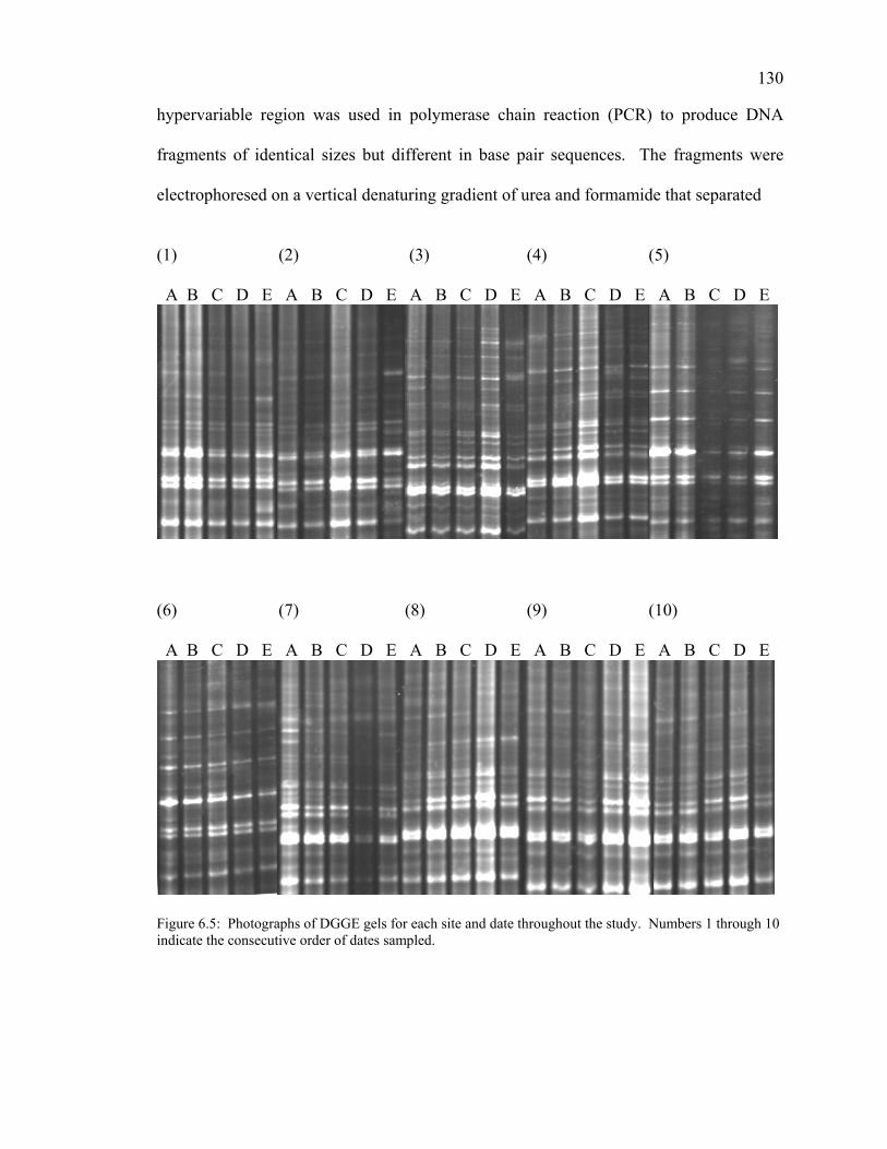
130
hypervariable region was used in polymerase chain reaction (PCR) to produce DNA
fragments of identical sizes but different in base pair sequences. The fragments were
electrophoresed on a vertical denaturing gradient of urea and formamide that separated
(1) (2) (3) (4) (5) A B C D E A B C D E A B C D E A B C D E A B C D E
(6) (7) (8) (9) (10) A B C D E A B C D E A B C D E A B C D E A B C D E
Figure 6.5: Photographs of DGGE gels for each site and date throughout the study. Numbers 1 through 10 indicate the consecutive order of dates sampled.
131
the fragments based on their mobilities due to differing sequences. Resulting fragments
are distinct bacterial OTUs (Muyzer et al. 1993; Muyzer and Smalla 1998; Schäfer and
Muyzer 2001). With ARISA, a primer set flanking the intergenic space between the 16s
and 23s rRNA genes was used in PCR. Amplified PCR fragments included this
intergenic space, which differs in both size and sequence for each OTU. Fragments were
separated on an automated fragment analysis system, in which an electropherogram
produced distinct peaks for each OTU (Fisher and Triplett 1999).
Molecular techniques, while powerful, have limitations that merit caution when
interpreting results. With PCR, the concentration of template DNA, PCR cycle
parameters (e.g. number of cycles, cycle temperatures), and multiple batches of PCR runs
(i.e. differing ingredient concentrations) may bias the final PCR product. These biases
may alter the proportions of genes present in the original gene pool (Casamayor et al.
2002). In DGGE, the primary limitation is that individual bands indicate OTUs
composing greater than 0.3-0.4% of the total community. Thus populations of low
abundance may go undetected in analyses (Reche et al. 2005). In addition, ‘double
banding’ may occur, in which more than one OTU is present in a single band (Sekiguchi
et al. 2001; Janse et al. 2004). Inter-gel variability resulting from variations in gradient
concentration may also confound results when comparing multiple DGGE gels (Schäfer
and Muyzer 2001). While few limitations have been reported with ARISA, there is a
possibility that two or more OTUs may share the same intergenic space length, thus a
single peak could represent more than one taxon, underestimating diversity
measurements (Fisher and Triplett 1999).
132
Significant variation occurred in the number of OTUs (richness) at the SWI
throughout the course of the study. However this difference did not correspond to a
specific season. High richness occurred under various mixing and stratified conditions.
The seasons that exhibited lowest richness occurred under two seasonal processes: 1)
complete anoxia and lowest observed redox potential during late summer stratification
(August and September 2004), and 2) winter mixing signified by coldest temperatures
(March 2004). Lower richness would be expected during times of stress such as low
redox potential or low temperature, however high richness occurred during February
2005 when temperatures were cold. No other studies have assessed bacterial richness at
the SWI, however some studies have assessed bacterial richness and diversity in oxic and
anoxic pelagic zones of various lakes. These studies either noted little change in seasonal
richness (i.e. Mono Lake, California) or higher richness in oxic waters (Lake
Sælenvannet, Norway) (Øvreås et al. 1997; Hollibaugh et al. 2001). An ARISA-based
study on several Wisconsin lakes of various trophic states noted substantial decreases in
pelagic bacterial richness during summer due to a clear-water phase, however these
differences were less pronounced in increasingly oligotrophic lakes (Yannarell et al.
2003).
No significant differences in Shannon-Weiner Diversity or Evenness were
observed based on relative peak areas produced by ARISA electorpherograms. High
evenness suggests that no single SWI bacterial population dominates the community.
Anoxia, low redox potential, and low temperatures are often considered stressful in terms
of most biota, which would lower evenness; however many bacteria are highly
specialized to occupy these habitats (Nealson 1997). In addition, some of the bacteria
133
detected in the ARISA analyses may have been present in samples, but dormant. This
may artificially inflate evenness measurements. Thus evenness does not imply function
of the community. It is possible that relatively few metabolically specific populations
conduct the bulk of the total community metabolism at any given time (Stevenson 1977).
Little seasonal difference in diversity does not suggest there are not seasonal
changes in the SWI bacterial composition. The Neighbor-Joining dendrogram (Figure
6.4) illustrates these differences. As a general observation, highest similarities appear
among the various sites after prolonged periods of stratification or mixing. This suggests
similar selective pressures at each site select for similar bacterial communities. During
transition periods (i.e. onset of stratification or onset of overturn) similarity decreases,
possibly as a function of heterogeneous selective pressures at the different sites. For
example, during the onset of stratification in May 2004, Sites D and E that have
undergone stratification and decreasing dissolved oxygen exhibit similar communities but
are dissimilar from Sites A, B, and C which are similar to one another because these sites
are still mixing.
Sulfate-reducing bacteria (SRB) are a diverse group of anaerobic bacteria that
reduce sulfate (SO42-) as a terminal electron acceptor in the presence of organic matter,
producing hydrogen sulfide (H2S). H2S is toxic to many organisms, contains antibiotic
properties, and causes aesthetic problems in reservoirs (Hines et al. 2002). Further,
sulfides can combine with various metals to produce metal sulfides in the sediments,
generating a characteristic black precipitate (Geets et al. 2006). Therefore elucidating the
diversity and distribution of these causative organisms (i.e. SRB) is important in
understanding rates and processes of sulfur cycling.
134
Common to all sulfate reducing bacteria is the dissimilatory sulfite reductase
(DSR) enzyme that catalyzes reduction of sulfite to sulfide. Thus the gene that codes for
the β-subunit of the DSR gene (dsrB) was used as a biomarker for diversity of SRB
(Wagner et al. 1998). While the dsrB gene is highly conserved, the SRB in which it is
contained are found in many diverse lineages including the δ subdivision of
Proteobacteria, some gram-positive bacteria, the subdivision Thermodesulfobacterium,
and the archaeal domain Euryarchaeota (Karr et al. 2005).
Although all SRB are anaerobic, presence of the DSR gene was found in all
samples under oxic and anoxic conditions. In addition, SRB richness was highest during
two winter mixing dates and lowest during a date corresponding to stratification and
anoxia. Recent studies have shown that active SRB have been found in oxic zones of
algal mats and biofilms (Dar et al. 2005). Other studies suggest that SRB violate the
paradigm of electron acceptors being utilized in the order of decreasing free energy
(Minz et al. 1999). Instead, SRB activity is possibly primarily controlled by the presence
of SO42-. Under aerobic conditions, dissolved oxygen and aerobic chemolithotrophic
bacteria would be expected to oxidize H2S to SO42-, thus providing a large pool of
potentially available SO42- to the SRB (Nealson 1997). These SRB could subsequently
reduce the SO42- under oxic conditions. If the sulfur-oxidizing aerobic chemolithotrophs
are more abundant and exhibit higher activities than SRB, equilibrium would shift to
SO42-. As oxygen becomes depleted due to stratification and aerobic bacterial
metabolism, the obligately aerobic sulfur oxidizers would decrease while the SRB would
continue to produce H2S. Thus H2S would accumulate under anaerobic conditions.
135
Conclusions Seasonal physicochemical changes at the SWI in Belton Reservoir have various
effects upon the SWI bacterial communities due to mixing and stratification. Total
bacterial abundance and diversity do not change on a spatial or seasonal scale. Total
concentration of SWI DNA shows significant decreases during onset of overturn and
onset of stratification. In addition, there are significant changes in the richness and
similarity of the bacterial communities among dates. While there are various exceptions,
higher similarity is associated with prolonged stratification or prolonged mixing.
Changes in richness did not follow a distinct seasonal pattern. Sulfate-reducing bacteria
are highly diverse, yet show greater richness under oxic conditions, implying that they
may be present but dormant. In contrast, SRB may be active under oxic conditions,
implying that they do not necessarily follow the traditional order of redox-specific
reductions.
Acknowledgments
This study was made possible by a University Research Committee Grant, Jack G.
and Norma Jean Folmar Grant, and Bob Gardner Memorial through Baylor University.
Further financial support was provided from a Texas River and Reservoir Management
Society Research Grant. We thank Christopher Filstrup and David Clubbs for field
assistance. We sincerely thank Dr. Diane Wycuff, Director of the Molecular Biosciences
Center, Baylor University, for support and assistance with the Beckman Sequencer,
thermocycler, image analysis software, and various molecular protocols. We also thank
Dr. Darrell Vodopich for gel photography assistance.
136
CHAPTER SEVEN
Conclusions
Sediment-water interfaces (SWIs) of monomictic, eutrophic reservoirs undergo
physical and chemical changes associated with mixing and stratification. Few other
ecosystems experience such an extensive habitat alteration on such a small spatial and
temporal scale. In addition, SWIs in reservoirs accumulate organic carbon at higher rates
than sediments of marine and other freshwater systems (Dean and Gorham 1998).
Bacteria metabolize much of this organic carbon, thus reservoir SWIs are unique
ecosystems for the study of bacterial community dynamics. The SWI of Belton
Reservoir presents such an ecosystem, thus it was used as the study location.
Various methods were used to investigate SWI bacterial community seasonal
dynamics, however the purpose of the study is summed into four basic ecological
questions: 1) How diverse is the (bacterial) community? 2) How active are the
community members? 3) Do community members preferentially feed on (i.e. uptake)
certain substrates? 4) How do internal and external (i.e. autochthonous and
allochthonous inputs) processes physically and chemically influence the habitat?
High seasonal SWI bacterial diversities were observed, and these seasonal
diversities were highly similar. High community diversities suggest establishment of
stable communities (Atlas and Bartha 1998). Unexpectedly this high diversity was
maintained under abiotic SWI stresses during onset of stratification and onset of overturn.
From the perspective of higher trophic levels, the SWI mixing and stratification
137
conditions are unfavorable to support stable communities. However specific bacterial
populations are readily able to exploit these environments marked by anoxia and low
redox potential. High, but similar, bacterial abundances were observed among all
seasons, further supporting evidence of high community stability.
A related, but more specific ecological question asks ‘how abundant are
individual taxa?’ This was explored with sulfate reducing bacteria (SRB). Higher
richness observed during oxic conditions challenges two widely-accepted principles: 1)
SRB are obligate anaerobes, only present during anoxic conditions, and 2) SRB are only
present when redox conditions are favorable. However, undetected micro-habitats may
exist that harbor SRB under their favored conditions. Yet, presence of these SRB
populations in previously undescribed habitats may redefine their niche.
The SWI bacterial community exhibited higher activity, production, and
generation time during anoxia and stratification. This evidence supports the diversity
data, suggesting that conditions often deemed ‘unfavorable’ are not at all unfavorable to
certain bacterial populations. The selective pressures brought upon by anoxia and low
redox potential gives way to bacterial populations that are readily able to exploit the SWI.
This concept is not new to microbial ecology, given Beijerinck’s principle, ‘everything is
everywhere, the environment selects’. However, classical community theory states that
there is a strong inverse relationship between diversity and productivity (Abrams 1995).
Results of this study appear to contradict this.
Because a spatial habitat gradient was built into the study design, widely varying
internal and external influences defined the chemical composition of the SWI.
Shallowest sites were defined by greater allochthonous inputs. Thus organic matter

138
composition varied among the sites, which potentially influence the taxa present. While
this investigation did not link presence of specific bacterial taxa to organic matter
composition, a further investigation examined the types of organic carbon preferred by
the bacteria under various mixing conditions. The marked differences in seasonal
utilization of specific substrates indicate that bacteria shift preference for certain
substrates based on their need of high carbon-containing or high nitrogen-containing
compounds. Alternatively, the types of organic matter present may select for
communities that optimally utilize the most easily oxidized substrate. The former
suggests that SWI bacteria are decidedly stenotolerant, while the latter suggests rapid
community succession occurs with changes in carbon inputs. Future investigations into
this phenomenon will clarify this uncertainty.

139
APPENDIX

140
APPENDIX
Publications Related to This Research
Chapter Two
Christian BW, Lind OT. In Press. Increased sediment-water interface bacterial [3H]-L-serine uptake and biomass production in a eutrophic reservoir during summer stratification. Archiv für Hydrobiologie.
Chapter Three
Christian BW, Lind OT. 2006. Key issues concerning Biolog use for aerobic and anaerobic freshwater bacterial community-level physiological profiling. International Review of Hydrobiology 91(3):257-268.
Chapter Four
Christian BW, Lind OT. In Press. Multiple carbon substrate utilization by bacteria at the sediment-water interface: seasonal patterns in a stratified eutrophic reservoir. Hydrobiologia.
141
BIBLIOGRAPHY
Abrams PA. 1995. Monotonic or unimodal diversity-productivity gradients: what does
competition theory predict? Ecology 76:2019-2027. Atlas R, Bartha R. 1998. Microbial ecology. 4th ed. Menlo Park: Benjamin Cummings.
694 p. Austen MC, Lambshead PJD, Hutchings PA, Boucher G, Snelgrove PVR, Heip C, King
G, Koike I, Smith C. 2002. Biodiversity links above and below the marine sediment-water interface that may influence community stability. Biodivers Conserv 11:113-136.
Balser TC, Kirchner JW, Firestone MK. 2002. Methodological variability in microbial
community level physiological profiles. Soil Sci Soc Am J 66:519-523. Bastviken D, Ejlertsson J, Tranvik L. 2001. Similar bacterial growth on dissolved
organic matter in anoxic and oxic lake water. Aquat Microb Ecol 24:41-49. Begon M, Harper JL, Townsend CR. 1996. Ecology: individuals, populations, and
communities. 3rd ed. Cambridge: Blackwell Science Ltd. 1068 p. Bell RT. 1993. Estimating production of heterotrophic bacterioplankton via
incorporation of tritiated thymidine. In: Kemp PF, Cole JJ, Sherr BF, Sherr EB, editors. Handbook of methods in aquatic microbial ecology. Boca Raton: CRC Press. p 495-512.
Bertilsson S, Tranvik LJ. 2000. Photochemical transformation of dissolved organic
matter in lakes. Limnol Oceanogr 45:753-762. Beutel MW 2003. Hypolimnetic anoxia and sediment oxygen demand in California
drinking water reservoirs. Lake and Res Manage 19:208-221. Bloem J, Bär-Gilissen MB, Cappenberg TE. 1986. Fixing, counting, and manipulation
of heterotrophic nanoflagellates. Appl Environ Microbiol 52:1266-1272. Bloesch J. 2004. Sedimentation and lake sediment formation. In: O’Sullivan PE,
Reynolds CS, editors. The lakes handbook: Volume 1 limnology and limnetic ecology. Malden: Blackwell. p 197-229.
Boström B, Jansson M, Forsberg C. 1982. Phosphorus release from lake sediments.
Arch Hydrobiol Beih Ergebn Limnol 18:5-99.
142
Boström B, Andersen JM, Fleischer S, Jansson M. 1988. Exchange of phosphorus across the sediment-water interface. Hydrobiologia 170:229-244.
Boudreau BP, Jørgensen BB. 2001. The benthic boundary layer: transport processes and
biogeochemistry. New York: Oxford University. 440 p. Braker G, Fesefeldt A, Witzel K. 1998. Development of PCR primer systems for
amplification of nitrite reductase genes (nirK and nirS) to detect denitrifying bacteria in environmental samples. Appl Environ Microbiol 64:3769-3775.
Brown MV, Schwalbach MS, Hewson I, Fuhrman JA. 2005. Coupling 16S-ITS rDNA
clone libraries and automated ribosomal intergenic spacer analysis to show marine microbial diversity: development and application to a time series. Environ Microbiol 7:1466-1479.
Brugger A, Reitner B, Kolar I, Quéric N, Harndl GJ. 2001. Seasonal and spatial
distribution of dissolved and particulate organic carbon and bacteria in the bank of an impounding reservoir on the Enns River, Austria. Fresh Biol 46:997-1016.
Brune A, Frenzel P, Cypionka H. 2000. Life at the oxic-anoxic interface: microbial
activities and adaptations. FEMS Microbiol Rev 24:691-710. Buesing N, Marxsen J. 2005. Theoretical and empirical conversion factors for
determining bacterial production in freshwater sediments via leucine incorporation. Limnol Oceanogr Meth 3:101-107.
Buffle J, de Vitre RR, Perret D, Leppard GG. 1989. Physicochemical characteristics of a
colloidal iron phosphate species formed at the oxic-anoxic interface of a eutrophic lake. Geochim Cosmochim Acta 53:399-408.
Butorin AN. 1989. The number and activity of microorganisms at the sediment water
interface of lakes. Arch Hydrobiol Beih Ergebn Limnol 33:259-263. Capone, DG. 2002. Microbial nitrogen cycling. In: Hurst CJ, Crawford RL, Knudsen
GR, McInerney MJ, Stetzenbach LD, editors. Manual of Environmental Microbiology. 2nd ed. Washington D.C.: ASM Press. p 439-449.
Cardinale M, Brusetti L, Quatrini P, Borin S, Puglia AM, Rizzi A, Zanardini E, Sorlini C,
Corselli C, Daffonchio D. 2004. Comparison of different primer sets for use in automated ribosomal intergenic spacer analysis of complex bacterial communities. Appl Environ Microbiol 70:6147-6156.
Casamayor EO, Pedrós-Alió C, Muyzer G, Amann R. 2002. Microheterogeneity in 16s
ribosomal DNA-defined bacterial populations from a stratified planktonic environment is related to temporal changes and to ecological adaptations. Appl Environ Microbiol 68:1706-1714.
143
Casper P. 1992. Methane production in lakes of different trophic state. Arch Hydrobiol Beih Ergebn Limnol 37:149-154.
Chin-Leo G. 2002. Bacterial secondary productivity. In: Hurst CJ, Crawford RL,
Knudsen GR, McInerney MJ, Stetzenbach LD, editors. Manual of Environmental Microbiology. 2nd ed. Washington D.C.: ASM Press. p 354-363.
Choi K, Dobbs FC. 1999. Comparison of two kinds of biolog microplates (GN and
ECO) in their ability to distinguish among aquatic microbial communities. J Microbiol Meth 36:203-213.
Christian BW, Early CN, Lind OT. 2002. Factors affecting bacterioplankton size and
abundance in anoxic hypolimnia. Verh Internat Verein Limnol 28:705-709. Christian BW, Lind OT. 2006. Key issues concerning biolog use for aerobic and
anaerobic freshwater bacterial community-level physiological profiling. Int Rev Hydrobiol 91:257-268.
Christian RR, Capone DG. 2002. Overview of issues in aquatic microbial ecology. In:
Hurst CJ, Crawford RL, Knudsen GR, McInerney MJ, Stetzenbach LD, editors. Manual of Environmental Microbiology. 2nd ed. Washington D.C.: ASM Press. p 323-328.
Classen AT, Boyle SI, Haskins KE, Overby SE, Hart SC. 2003. Community-level
physiological profiles of bacteria and fungi: plate type and incubation temperature influences on contrasting soils. FEMS Microbiol Ecol 44:319-328.
Cole JJ, Pace ML. 1995. Bacterial secondary production in oxic and anoxic freshwaters.
Limnol Oceanogr 40:1019-1027. Danovaro R, Croce ND, Fabiano M. 1998. Biochemical composition of particulate
organic matter and bacterial dynamics at the sediment-water interface in a Mediterranean seagrass system. Hydrobiologia 363:241-251.
Dar SA, Kuenen JG, Muyzer G. 2005. Nested PCR-denaturing gradient gel
electrophoresis approach to determine the diversity of sulfate-reducing bacteria in complex microbial communities. Appl Environ Microbiol 71:2325-2330.
Dean WE. 1974. Determination of carbonate and organic matter in calcareous sediments
and sedimentary rocks by loss on ignition: comparison with other methods. J Sed Petr 44:242-248.
Dean WE, Gorham E. 1998. Magnitude and significance of carbon burial in lakes,
reservoirs, and peatlands. Geology 26: 535-538.
144
Dean WE. 1999. The carbon cycle and biogeochemical dynamics in lake sediments. J Paleolim 21:375-393.
Dell’Anno A, Corinaldesi C. 2004. Degradation and turnover of extracellular DNA in
marine sediments: ecological and methodological considerations. Appl Environ Microbiol 70:4384-4386.
Ding H, Sun M. 2005. Biochemical degradation of algal fatty acids in oxic and anoxic
sediment-seawater interface systems: effects of structural association and relative roles of aerobic and anaerobic bacteria. Mar Chem 93:1-19.
dos Santos Furtado AL, Casper P. 2000. Different methods for extracting bacteria from
freshwater sediment and a simple method to measure bacterial production in sediment simples. J Microbiol Meth 41:249-257.
Ducklow H. 2000. Bacterial production and biomass in the oceans. In: Kirchman DL,
editor. Microbial ecology of the oceans. New York: Wiley. p 85-120. Ellery WN, Schleyer MH. 1984. Comparison of homogenization and ultrasonication as
techniques in extracting attached sedimentary bacteria. Mar Ecol Prog Ser 15:247-250.
Ferrara-Guerrero MJ, Marty DG, Bianchi A. 1993. Isolation and enumeration of
anaerobic and microaerophilic bacteria in aquatic habitats. In: Kemp PF, Cole JJ, Sherr BF, Sherr EB, editors. Handbook of methods in aquatic microbial ecology. Boca Raton: CRC Press. p 9-20.
Findlay RH, Trexler MB, Guckert JB, White DC. 1990. Laboratory study of disturbance
in marine sediments: response of a microbial community. Mar Ecol Prog Ser 62:121-133.
Findlay S. 1993. Thymidine incorporation into DNA as an estimate of sediment
bacterial production. In: Kemp PF, Cole JJ, Sherr BF, Sherr EB, editors. Handbook of methods in aquatic microbial ecology. Boca Raton: CRC Press. p 505-508.
Fisher MM, Triplett EW. 1999. Automated approach for ribosomal intergenic spacer
analysis of microbial diversity and its application to freshwater bacterial communities. Appl Environ Microbiol 65:4630-4636.
Forja JM, Gómez-Parra A. 1998. Measuring nutrient fluxes across the sediment-water
interface using benthic chambers. Mar Ecol Prog Ser 164:95-105. Gächter R, Meyer JS, Mares A. 1988. Contribution of bacteria to release and fixation of
phosphorus in lake sediments. Limnol Oceanogr 33:1542-1558.
145
Gächter R, Meyer JS. 1993. The role of microorganisms in mobilization and fixation of phosphorus in sediments. Hydrobiologia 253:103-121.
Gamo M, Shoji T. 1999. A method of profiling microbial communities based on a most-
probable-number assay that uses BIOLOG plates and multiple sole carbon sources. Appl Environ Microbiol 65:4419-4424.
Gantzer CJ, Stefan HG. 2003. A model of microbial activity in lake sediments in
response to periodic water-column mixing. Water Res 37:2833-2846. Garland JL. 1997. Analysis and interpretation of community-level physiological profiles
in microbial ecology. FEMS Microbiol Ecol 24:289-300. Garland JL, Mills AL. 1991. Classification and characterization of heterotrophic
microbial communities on the basis of patterns of community-level-sole-carbon-source utilization. Appl Environ Microbiol 57:2351-2359.
Geets J, Borremans B, Diels L, Springael D, Vangronsveld J, van der Lelie D,
Vanbroekhoven K. 2006. DsrB gene-based DGGE for community and diversity surveys of sulfate-reducing bacteria. J Microbiol Meth 66:194-205.
Gilmour CC, Leavitt ME, Shiaris MP. 1990. Evidence against incorporation of
exogenous thymidine by sulfate-reducing bacteria. Limnol Oceanogr 35:1401- 1409.
Glimm E, Heuer H, Engelen B, Smalla K, Backhaus H. 1997. Statistical comparisons of
community catabolic profiles. J Microbiol Meth 30:71-80. Golterman HL. 2001. Phosphate release from anoxic sediments or ‘what did Mortimer
really write?’ Hydrobiologia 450:99-106. Gotelli NJ, Ellison AM. 2004. A primer of ecological statistics. Sunderland: Sinauer
Associates. 510 p. Grebe TW, Stock J. 1998. Bacterial chemotaxis: the five sensors of a bacterium Curr
Biol 8:R154-R157. Grover JP, Chrzanowski TH. 2000. Seasonal patterns of substrate utilization by
bacterioplankton: case studies in four temperate lakes of different latitudes. Aquat Microb Ecol 23:41-54.
Haack SK, Garchow H, Klug MJ, Forney LJ. 1995. Analysis of factors affecting the
accuracy, reproducibility, and interpretation of microbial community carbon source utilization patterns. Appl Environ Microbiol 61:1458-1468.
146
Hackett CA, Griffiths BS. 1997. Statistical analysis of the time-course of Biolog substrate utilization. J Microbiol Meth 30:63-69.
Hallin S, Lindgren P. 1999. PCR detection of genes encoding nitrite reductase in
denitrifying bacteria. Appl Environ Microbiol 65:1652-1657. Harris D, Horwáth WR, van Kessel C. 2001. Acid fumigation of soils to remove
carbonates prior to total organic carbon or carbon-13 isotopic analysis. Soil Sci Am J 65:1853-1856.
Harrison MJ, Pacha RE, Morita RY. 1972. Solubilization of inorganic phosphates by
bacteria isolated from Upper Klamath lake sediment. Limnol Oceanogr 17:50-57. Heinen EA, McManus J. 2004. Carbon and nutrient cycling at the sediment-water
boundary in western Lake Superior. J Great Lakes Res 30:113-132. Hewson I, Fuhrman JA. 2004. Richness and diversity of bacterioplankton species along
an estuarine gradient in Moreton Bay, Australia. Appl Environ Microbiol 70:3425-3433.
Higashino M, Stefan HG. 2004. Diffusive boundary layer development above a
sediment-water interface. Water Environ Res 76:292-300. Hines ME, Visscher PT, Devereux R. 2002. Sulfur cycling. In: Hurst CJ, Crawford RL,
Knudsen GR, McInerney MJ, Stetzenbach LD, editors. Manual of Environmental Microbiology. 2nd ed. Washington D.C.: ASM Press. p 427-438.
Hobbie JE, Daley RJ, Jasper S. 1977. Use of Nuclepore filters for counting bacteria by
fluorescence microscopy. Appl Environ Microbiol 33:1225-1228. Hodell DA, Schelske CL. 1998. Production, sedimentation, and isotopic composition of
organic matter in Lake Ontario. Limnol Oceanogr 43:200-214. Hoefs J. 2004. Stable isotope geochemistry. 5th edition. Berlin: Springer. 244 p. Hollibaugh JT, Azam F. 1983. Microbial degradation of dissolved proteins in seawater.
Limnol Oceanogr 28:1104-1116. Hollibaugh JT, Wong PS, Bano N, Pak SK, Prager EM, Orrego C. 2001. Stratification
of microbial assemblages in Mono Lake, California, and response to a mixing event. Hydrobiologia 466:45-60.
Horne A, Goldman C. 1994. Limnology. 2nd edition. New York: McGraw-Hill. 480 p.
147
Heuer H, Weiland G, Schönfeld J, Schönwälder A, Gomes NCM, Smalla K. 2001. Bacterial community profiling using DGGE or TGGE analysis. In: Rochelle PA, editor. Environmental molecular microbiology: protocols and applications. Norwich: Horizon Scientific. p 177-190.
Huettel M, Roy H, Precht E, Ehrenhauss S. 2003. Hydrodynamical impact on
biogeochemical processes in aquatic sediments. Hydrobiologia 494:231-236. Hulbert MH, Bennett RH, Baerwald RJ, Long RL, Curry KJ, Curry AL, and Abril MT.
2002. Observations of the sediment-water interface: marine and fresh water environments. Mar Geores Geotechnol 20:255-274.
Hyacinthe C, Bonneville S, Van Cappellen P. 2006. Reactive iron (III) in sediments:
chemical versus microbial extractions. Geochim Cosmochim Acta 70:4166-4180. Insam H, Goberna M. 2004. Use of Biolog for the community level physiological
profiling (CLPP) of environmental samples. In: Kowalchuk GA, deBruijn FJ, Head IM, Akkermans AD, vanElsas JD, editors. Molecular microbial ecology manual. 2nd ed. Berlin: Springer. p 853-860.
Jahnke RA, Craven DB. 1995. Quantifying the role of heterotrophic bacteria in the
carbon cycle: a need for respiration rate measurements. Limnol Oceanogr 40:436-441.
Janse I, Bok J, Zwart G. 2004. A simple remedy against artifactual double bands in
denaturing gradient gel electrophoresis. J Microbiol Meth 57:279-281. Johnstone BH, Jones RD. 1989. A study on the lack of [methyl-3H] thymidine uptake
and incorporation by chemolithotrophic bacteria. Microb Ecol 18:73-77. Jones JG. 1979. Microbial activity in lake sediments with particular reference to
electrode potential gradients. J Gen Microbiol 115:19-26. Jones RD. 2002. Phosphorus cycling. In: Hurst CJ, Crawford RL, Knudsen GR,
McInerney MJ, Stetzenbach LD, editors. Manual of Environmental Microbiology. 2nd ed. Washington D.C.: ASM Press. p 450-455.
Jonsson A, Meili M, Bergström A, Jansson M. 2001. Whole-lake mineralization of
allochthonous and autochthonous organic carbon in a large humic lake (Örträsket, N. Sweden). Limnol Oceanogr 46:1691-1700.
Karr EA, Sattley WM, Rice MR, Jung DO, Madigan MT, Achenbach LA. 2005.
Diversity and distribution of sulfate-reducing bacteria in permanently frozen Lake Fryxell, McMurdo Dry Valleys, Antarctica. Appl Environ Microbiol 71:6353-6359.
148
Kelly CA, Rudd JWM, Schindler DW. 1988. Carbon and electron flow via methanogenesis, SO4
2-, NO3-, Fe3+, and Mn4+ reduction in the anoxic hypolimnia
of three lakes. Arch Hydrobiol Beih Ergebn Limnol 31:333-344. Kelly DP, Wood AP. 1998. Microbes of the sulfur cycle. In: Burlage RS, Atlas R,
Stahl D, Geesey G, Sayler G, editors. Techniques in microbial ecology. New York: Oxford University Press. p 31-57.
King GM. 2002. Radiotracer (14C and 3H) assays for benthic microbial organic matter
transformations. In: Hurst CJ, Crawford RL, Knudsen GR, McInerney MJ, Stetzenbach LD, editors. Manual of Environmental Microbiology. 2nd ed. Washington D.C.: ASM Press. p 419-426.
Kirchman D, K’nees E, Hodson R. 1985. Leucine incorporation and its potential as a
measure of protein synthesis by bacteria in natural aquatic systems. Appl Environ Microbiol 49:599-607.
Kirchman DL. 1993. Leucine incorporation as a measure of biomass production by
heterotrophic bacteria. In: Kemp PF, Cole JJ, Sherr BF, Sherr EB, editors. Handbook of methods in aquatic microbial ecology. Boca Raton: CRC Press. p 509-512.
Kirchman D. 2001. Measuring bacterial biomass production and growth rates from
leucine incorporation in natural aquatic environments. In: Paul JH, editor. Methods in microbiology Volume 30. San Diego: Academic Press. p. 227-236.
Kirk JL, Beaudette LA, Hart M, Moutoglis P, Klironomos JN, Lee H, Trevors JT. 2004.
Methods of studying soil microbial diversity. J Microbiol Meth 58:169-188. Kirk RE. 1999. Statistics: an introduction, 4th ed. Fort Worth: Harcourt Brace. 755 p. Konopka A, Oliver L, Turco Jr RF. 1998. The use of carbon substrate utilization
patterns in environmental and ecological microbiology. Microb Ecol 35:103-115. Kostka J, Nealson KH. 1998. Isolation, cultivation and characterization of iron- and
manganese- reducing bacteria. In: Burlage RS, Atlas R, Stahl D, Geesey G, Sayler G, editors. Techniques in microbial ecology. New York: Oxford University Press. p 59-78.
Kuwae T, Hosokawa Y. 1999. Determination of abundance and biovolume of bacteria
in sediments by dual staining with 4`6-Diamidino-2-phenylindole and acridine orange: relationship to dispersion treatment and sediment characteristics. Appl Environ Microbiol 65:3407-3412.
Lee S, Fuhrman JA. 1987. Relationships between biovolume and biomass of naturally
derived marine bacterioplankton. Appl Environ Microbiol 52:1298-1303.
149
Lehmann MF, Bernasconi SM, Barbieri A, McKenzie JA. 2002. Preservation of organic matter and alteration of its carbon and nitrogen isotope composition during simulated and in situ early sedimentary diagenesis. Geochim Cosmochim Acta 66: 3573-3584.
Lepš J, Šmilauer P. 2002. Multivariate analysis of ecological data using CANOCO.
Cambridge: Cambridge University Press. 269 p. Liikanen A, Martikainen PJ. 2003. Effect of ammonium and oxygen on methane and
nitrous oxide fluxes across sediment-water interface in a eutrophic lake. Chemosphere 52:1287-1293.
Lind OT. 1984. Phytoplankton population patterns and trophic state relationships in an
elongate reservoir. Verh Internat Verein Limnol 22:1465-1469. Lind OT, Dávalos-Lind L. 1991. Association of turbidity and organic carbon with
bacterial abundance and cell size in a large, turbid, tropical lake. Limnol Oceanogr 36:1200-1208.
Lindstrom JE, Barry RP, Braddock JF. 1998. Microbial community analysis: a kinetic
approach to constructing potential c source utilization patterns. Soil Biol Biochem 30:231-239.
Liu WT, Stahl DH. 2002. Molecular approaches for the measurement of density,
diversity, and phylogeny. In: Hurst CJ, Crawford RL, Knudsen GR, McInerney MJ, Stetzenbach LD, editors. Manual of Environmental Microbiology. 2nd ed. Washington D.C.: ASM Press. p 114-134.
Lovley DR, Phillips EJP. 1988. Novel mode of microbial energy metabolism: organic
carbon oxidation coupled to dissimilatory reduction of iron or manganese. Appl Environ Microbiol 54:1472-1480.
MacGregor BJ. 1999. Molecular approaches to the study of aquatic microbial
communities. Curr Opin Biotech 10:220-224. Madigan MT, Martinko J, Parker J. 1997. Brock Biology of Microorganisms, 8th ed.
Upper Saddle River: Prentice Hall. 1088 p. McMahon JW. 1969. The annual and diurnal variation in the vertical distribution of
acid-soluble ferrous and total iron in a small dimictic lake. Limnol Oceanogr 14:357-367.
Meyers PA, Teranes JL. 2001. Sediment organic matter. In: Last WM, Smol JP,
editors. Tracking environmental change using lake sediments. Volume 2: physical and geochemical methods. Dordrecht: Kluwer. p 239-269.

150
Mills AL. 2002. Metal requirements and tolerance. In: Hurst CJ, Crawford RL, Knudsen GR, McInerney MJ, Stetzenbach LD, editors. Manual of Environmental Microbiology. 2nd ed. Washington D.C.: ASM Press. p 456-465.
Mills AL, Garland JL. 2002. Application of physiological profiles to assessment of
community properties. In: Hurst CJ, Crawford RL, Knudsen GR, McInerney MJ, Stetzenbach LD, editors. Manual of Environmental Microbiology. 2nd ed. Washington D.C.: ASM Press. p 135-146.
Minz D, Flax JL, Green SJ, Muyzer G, Cohen Y, Wagner M, Rittman BE, Stahl DA.
1999. Diversity of sulfate-reducing bacteria in oxic and anoxic regions of a microbial mat characterized by comparative analysis of dissimilatory sulfite reductase genes. Appl Environ Microbiol 65:4666-4671.
Mortimer CH. 1941. The exchange of dissolved substances between mud and water in
lakes, I and II. J Ecol 29:280-329. Mortimer CH. 1942. The exchange of dissolved substances between mud and water in
lakes, III and IV. J Ecol 30:147-201. Mortimer CH. 1971. Chemical exchanges between sediments and water in the great
lakes—speculations on probable regulatory mechanisms. Limnol Oceanogr 16:387-404.
Murrell MC, Hollibaugh JT, Silver MW, Wong PS. 1999. Bacterioplankton dynamics in
northern San Francisco Bay: role of particle association and seasonal freshwater flow. Limnol Oceanogr 44:295-308.
Muyzer G, DeWaal EC, Uitterlinden AG. 1993. Profiling of complex microbial
populations by denaturing gradient gel electrophoresis analysis of polymerase chain reaction-amplified genes coding for 16S rRNA. Appl Environ Microbiol 59:695-700.
Muyzer G, Smalla K. 1998. Application of denaturing gradient gel electrophoresis
(DGGE) and temperature gradient gel electrophoresis (TGGE) in microbial ecology. Antonie van Leeuwenhoek 73:127-141.
Nealson KH. 1997. Sediment bacteria: who’s there, what are they doing, and what’s
new? Annu Rev Earth Planet Sci 25:403-434. Nealson, KH, Stahl DA. 1997. Microorganisms and biogeochemical cycles: what can
we learn from layered microbial communities? In: Banfield JF, Nealson KH, editors. Geomicrobiology: Interactions between microbes and minerals. Washington D.C.: Mineralogical Society of America. p 5-34.

151
Novitsky JA. 1983. Microbial activity at the sediment-water interface in Halifax Harbor, Canada. Appl Environ Microbiol 45:1761-1766.
O’Loughlin EJ, Chin Y. 2004. Quantification and characterization of dissolved organic
carbon and iron in sedimentary porewater from Green Bay, WI, USA. Biogeochemistry 71:371-386.
Øvreås L, Forney L, Daae FL, Torsvik V. 1997. Distribution of bacterioplankton in
meromictic Lake Sælenvannet, as determined by denaturing gradient gel electrophoresis of PCR-amplified gene fragments coding for 16S rRNA. Appl Environ Microbiol 63:3367-3373.
Peres-Neto PR, Jackson DA, Somers KM. 2003. Giving meaningful interpretation to
ordination axes: assessing loading significance in principal component analysis. Ecology 84:2347-2363.
Pettine M, Patrolecco L, Manganelli M, Capri S, Farrace MG. 1999. Seasonal variations
of dissolved organic matter in the northern Adriatic Sea. Mar Chem 64:153-169. Pomeroy LR. 1974. The ocean’s food web: a changing paradigm. BioScience 24:499-
504. Porter KG, Feig YS. 1980. The use of DAPI for identifying and counting aquatic
microflora. Limnol Oceanogr 25:943-948. Preston-Mafham J, Boddy L, Randerson PF. 2002. Analysis of microbial community
functional diversity using sole-carbon-source utilization profiles – a critique. FEMS Microbiol Ecol 42:1-14.
Qiu, L, Williams DF, Gvorzdkov A, Karabanov E, Shimaraeva M. 1993. Biogenic silica
accumulation and paleoproductivity in the northern basin of Lake Baikal during the Holocene. Geology 21:25-28.
Qu W, Morrison RJ, West RJ, Su C. 2005. Diagenetic stoichiometry and benthic
nutrient fluxes at the sediment-water interface of Lake Illawarra, Australia. Hydrobiologia 537:249-264.
Ramsay AJ. 1984. Extraction of bacteria from soil: efficiency of shaking or
ultrasonication as indicated by direct counts and autoradiography. Soil Biol Biochem 16:475-481.
Reche I, Pulido-Villena E, Morales-Baquero R, Casamayor EO. 2005. Does ecosystem
size determine aquatic bacterial richness? Ecology 86:1715-1722.
152
Reeck G. 1973. Amino acid compositions of selected proteins. In: Laskin AI, Lechevalier HA, editors. Handbook of Microbiology, Volume 2, microbial composition. Boca Raton: CRC Press. p 15-29.
Reeck GR, Fisher L. 1973. A statistical analysis of the amino acid compositions of
proteins. Int J Peptide Protein Res 5:109-117. Rosenstock B, Simon M. 2003. Consumption of dissolved amino acids and
carbohydrates by limnetic bacterioplankton according to molecular weight fractions and proportions bound to humic matter. Microb Ecol 45:433-443.
Rosenstock B, Zwisler W, Simon M. 2005. Bacterial consumption of humic and non-
humic low and high molecular weight DOM and the effect of solar irradiation on the turnover of labile DOM in the southern ocean. Microb Ecol 50:90-101.
Rosselló-Mora R, Thamdrup B, Schäfer H, Weller R, Amann R. 1999. The response of
the microbial community of marine sediments to organic carbon input under anaerobic conditions. System Appl Microbiol 22:237-248.
Rutherford K. 1998. Hypolimnetic oxygen decline and the hypolimnetic bacterial
community [master’s thesis]. Waco (TX): Baylor University. 71 p. Sala MM, Arin L, Balagué V, Felipe J, Guadayol O, Vaqué D. 2005. Functional
diversity of bacterioplankton assemblages in western antarctic seawaters during late spring. Mar Ecol Progr Ser 292:13-21.
Sala MM, Pinhassi J, Gasol JM. 2006. Estimation of bacterial use of dissolved organic
nitrogen compounds in aquatic ecosystems using Biolog plates. Aquat Microb Ecol 42:1-5.
Santschi P, Höhener P, Benoit G, Buchholtz-ten Brink M. 1990. Chemical processes at
the sediment-water interface. Mar Chem 30:269-315. Schäfer H, Muyzer G. 2001. Denaturing gradient gel electrophoresis in marine
microbial ecology. In: Paul JH, editor. Methods in microbiology Volume 30. San Diego: Academic Press. p 425-468.
Schallenberg M, Kalff J. 1993. The ecology of sediment bacteria in lakes and
comparisons with other aquatic ecosystems. Ecology 74:919-934. Schultz GE, Ducklow HW. 2000. Changes in bacterioplankton metabolic capabilities
along a salinity gradient in the York River estuary, Virginia, USA. Aquat Microb Ecol 22:163-174.
Seiter K, Hensen C, Zabel M. 2005. Benthic carbon mineralization on a global scale.
Glob Biogeochem Cyc 19:GB1010.

153
Sekiguchi H, Tomioka N, Nakahara T, Uchiyama H. 2001. A single band does not always represent single bacterial strains in denaturing gradient gel electrophoresis analysis. Biotech Letters 23:1205-1208.
Servais P. 1995. Measurement of the incorporation rates of four amino acids into
proteins for estimating bacterial production. Microb Ecol 29:115-128. Sherr E, Sherr B. 1988. Role of microbes in pelagic food webs: a revised concept.
Limnol Oceanogr 33:1225-1227. Simon M, Azam F. 1989. Protein content and protein synthesis rates of planktonic
marine bacteria. Mar Ecol Prog Ser 51:201-213. Sinsabaugh RL, Findlay S, Franchini P, Fischer D. 1997. Enzymatic analysis of riverine
bacterioplankton production. Limnol Oceanogr 42:29-38. Sinsabaugh RL, Foreman CM. 2001. Activity profiles of bacterioplankton in a eutrophic
river. Freshwater Biol 46:1239-1249. Smalla K, Wachtendorf U, Heuer H, Liu W, Forney L. 1998. Analysis of Biolog GN
substrate utilization patterns by microbial communities. Appl Environ Microbiol 64:1220-1225.
Song, J, Luo Y, Zhao Q, Christie P. 2004. Microcosm studies on anaerobic phosphate
flux and mineralization of lake sediment organic carbon. J Environ Qual 33:2353-2356.
Stevenson LH. 1977. A case for bacterial dormancy in aquatic ecosystems. Microb Ecol
4:127-133. Stumm W. 2004. Chemical processes regulating the composition of lake waters. In:
O’Sullivan PE, Reynolds CS, editors. The lakes handbook: volume 1 limnology and limnetic ecology. Malden: Blackwell. p 79-106.
Sweerts JRA, Bär-Gilissen M, Cornelese AA, Cappenberg TE. 1991. Oxygen-
consuming processes at the profundal and littoral sediment-water interface of a small meso-eutrophic lake (Lake Vechten, The Netherlands). Limnol Oceanogr 36:1124-1133.
Syväranta J, Hämäläinen H, Jones RI. 2006. Within-lake variability in carbon and
nitrogen stable isotope signatures. Fresh Biol 51:1090-1102. Tam L, Kevan PG, Trevors JT. 2003. Viable bacterial biomass and functional diversity
in fresh and marine waters in the canadian arctic. Polar Biol 26:287-294.

154
Tammert H, Kisand V, Nõges T. 2005. Bacterioplankton abundance and activity in a small hypertrophic stratified lake. Hydrobiologia 547:83-90.
Tankéré SPC, Bourne DG, Muller FLL, Torsvik V. 2002. Microenvironments and
microbial community structure in sediments. Environ Microbiol 4:97-105. Taroncher-Oldenburg G, Griner EM, Francis CA, Ward BB. 2003. Oligonucleotide
microarray for the study of functional gene diversity in the nitrogen cycle in the environment. Appl Environ Microbiol 69:1159-1171.
ter Braak CJF, Šmilauer P. 2002. CANOCO reference manual and CanoDraw for
Windows user’s guide: software for canonical community ordination (version 4.5). Ithaca: Microcomputer Power. 500 p.
Thornton SF, McManus J. 1994. Applications of organic carbon and nitrogen stable
isotope and C/N ratios as source indicators of organic matter provenance in estuarine systems: evidence from the Tay Estuary, Scotland. Estuar Coast Shelf Sci 38:219-233.
Tomaszek JA, Czerwieniec E. 2003. Denitrification and oxygen consumption in bottom
sediments: factors influencing rates of the processes. Hydrobiologia 504:59-65. Torsvik V, Daae FL, Sandaa RA, Øvreås L. 1998. Novel techniques for analysing
microbial diversity in natural and perturbed environments. J Biotech 64:53-62. Torsvik V, Øvreås L, Thingstad TF. 2002. Prokaryotic diversity—magnitude, dynamics,
and controlling factors. Science 296:1064-1066. Tranvik LJ, Olofsson H, Bertilsson S. 1999. Photochemical effects on bacterial
degradation of dissolved organic matter in lake water. In: Bell CR, Brylinsky M, and Johnson-Green P, editors. Microbial Biosystems: New Frontiers, Proceedings of the 8th International Symposium on Microbial Ecology. Halifax: Atlantic Canada Society for Microbial Ecology.
[USACE] United States Army Corps of Engineers, Fort Worth District. 2002 Apr.
Bosque and Leon River Watersheds Study. 193 p. Van Mooy B, MacGregor B, Hollander D, Nealson K, Stahl D. 2001. Evidence for tight
coupling between active bacteria and particulate organic carbon during stratification of Lake Michigan. Limnol Oeceanogr 46:1202-1208.
Vestal JR, White DC. 1989. Lipid analysis in microbial ecology: quantitative
approaches to the study of microbial communities. BioScience 39:535-541. Vreča P. 2003. Carbon cycling at the sediment-water interface in a eutrophic mountain
lake (Jezeru na Planini pri Jezeru, Slovenia). Org Geochem 34:671-680.
155
Wagner M, Roger AJ, Flax JL, Brusseau GA, Stahl DA. 1998. Phylogeny of dissimilatory sulfite reductases supports an early origin of sulfate respiration. J Bacterio 180:2975-2982.
Wetzel R.G. 2001. Limnology: lake and river ecosystems. 2nd edition. San Diego:
Academic Press. 850 p. Wheeler PA, Kirchman DL. 1986. Utilization of inorganic and organic nitrogen by
bacteria in marine systems. Limnol Oceanogr 31:998-1009. White D. 1999. The physiology and biochemistry of prokaryotes. New York: Oxford
University Press. White DC, Davis WM, Nickels JS, King JD, Bobbie RJ. 1979. Determination of the
sedimentary microbial biomass by extractible lipid phosphate. Oecologia 40:51-62.
White DC, Ringelberg DB. 1998. Signature lipid biomarker analysis. In: Burlage RS,
Atlas R, Stahl D, Geesey G, Sayler G, editors. Techniques in microbial ecology. New York: Oxford University Press. p 255-272.
Wirtz KW. 2003. Control of biogeochemical cycling by mobility and metabolic
strategies of microbes in the sediments: an integrated model study. FEMS Microbiol Ecol 46:295-306.
Yannarell AC, Kent AD, Lauster GH, Kratz TK, Triplett EW. 2003. Temporal patterns
in bacterial communities in three temperate lakes of different trophic status. Microb Ecol 46:391-405.
Zhang T, Fang HHP. 2000. Digitization of DGGE (denaturing gradient gel
electrophoresis) profile and cluster analysis of microbial communities. Biotechnology Letters 22:399-405.