Dynamic Simulation of High Purity
Distillation Column
by
Abdullah Baihaqi Adzha bin Zubir
Dissertation submitted in partial fulfilment of
the requirements for the
Bachelor of Engineering (Hons)
(Chemical Engineering)
JUNE 2009
Universiti Teknologi PETRONAS
Bandar Seri Iskandar
31750 Tronoh
Perak Darul Ridzuan
Approve by:
CERTIFICATION OF APPROVAL
Dynamic Simulation of High Purity
Distillation Column
by
Abdullah Baihaqi Adzha bin Zubir
A project dissertation submitted to the
Chemical Engineering Programme
Universiti Teknologi PETRONAS
in partial fulfillment of the requirement for the
BACHELOR OF ENGINEERING (Hons)
(CHEMICAL ENGINEERING)
(AP DR RAMASAMY MARAPPAGOUNDER)
UNIVERSITI TEKNOLOGI PETRONAS
TRONOH, PERAK
11
JUNE 2009
CERTIFICATION OF ORIGINALITY
This is to certify that I am responsible for the work submitted in this project, that the
original work is my own except as specified in the references and
acknowledgements, and that the original work contained herein have not been
undertaken or done by unspecified sources or persons.
JEfAC(ABDULLAH BAIHAQI ADZHA BIN ZUBIR)
in
ABSTRACT
This report presents a research study on dynamic simulation ofhigh purity distillation column via
MATLAB. The dynamic nature and the nonlinear behaviour ofdistillation equipment pose
challenging control system design when products of constant purity are to be recovered.
Several alternative column configurations and operating policies have been studied.
However, issues related to the online operation of such process have not been properly
addressed. The present work describes the investigation with experimental verification of
computer based control strategies to distillation. The scope ofwork for the project is to
conduct a literature review on dynamic behaviour of high purity distillation column The
study provides a method ofstudying the dynamic behaviour of column comprising the steps
of: a) generating a principle steady state and dynamic model corresponding to the distillation
process; b) simulating the dynamic model for different operating condition via MATLAB; c)
Develop output trend towards changes in input via Pseudo Random Binary Sequence
(PRBS); e) Develop step response of first order process ; and f) obtain the gain and time
constant for any changes ofcolumn operating condition through first order process response
for control purposes A distillation model with 41-stage column with the overhead condenser
as stage 1, the feed tray as stage 21 and the reboiler as stage 41 is used. The findings show
that the models represent an ideal distillation column. All the research and findings obtained
will be used to improve the overall performance of the column as well as to improve the
quality of the product and maximise profitability. The successful outcome of this project will
be a great helping hand for industrial application.
IV
ACKNOWLEDGEMENT
First and foremost, the author would like to give my sincere thanks to ALLAH SWT, the
almighty God, the source of my life and hope for giving me the strength and wisdom to
complete the research.
The author is most grateful to his supervisor AP Dr. Ramasamy Marappagounder for being
such an understanding and good supervisor throughout one year of final year project. Many
times, his patience and constant encouragement has steered me to the right direction. His
continuous guidance and knowledge from initial start of the project until final completion did
help the author in choosing the correct solution for every problem occurred.
Not forgotten to Chemical Engineering Lecturers for their help in sharing their valuable
experiences and knowledge in enhancing the student understanding on the topic of the
project. The author would like also express his gratitude to the Graduate Assistance from
UTP, MtTotok and MrXemma for their effort in helping and providing the author with the
knowledge and assistance for this research.
At last and most importantly, the author would like to thank his family, friends and everyone
who have contributes in this project and gave motivation and encouragement so that the
author able to complete this project.
Thank you.
CHAPTER 1:
TABLE OF CONTENTS
INTRODUCTION
1.1 Background of Study
1.2 Problem statement
1.3 Objectives
1.4 Scope ofWork
CHAPTER 2: THEORY
2.1 Distillation Process
2.2 The Column
2.3 Column Variables and Their Pairing
2.4 Composition Control
2.5 Dynamic Modelling
CHAPTER 3: MET HODOLOGY
3.1 Generating a Principle Dynamic Model Corresponding
to the Distillation Process
3.2 Simulatingthe Dynamic Model for Different Operating
Condition via MATLAB
3.3 Output Trend Towards Changes in Input via Pseudo
Random Binary Sequence (PRBS)
3.4 Response of First Order Process
3.5 Step Response of First Order Process
VI
4
6
8
10
11
13
17
18
19
19
CHAPTER 4:
CHAPTERS:
REFERENCES
APPENDICES
RESULT AND DISCUSSION
4.1 Steady State Operation of a 41-Stage Column
4.2 Dynamic Operationofa 41-Stage Column
4.3 Output Trend Towards Changes in Input via Pseudo
Random Binary Sequence (PRBS)
4.4 Step Response ofFirst Order Process
CONCLUSION AND RECOMMENDATION
VII
21
24
26
28
33
34
35
LIST OF FIGURES
LIST OF HLUSTRATION
Figure 2.1 Illustration of a tray-type distillation tower 5
Figure 2.2 Left : The vapor recompression system uses recovered heat. 6
Right: The pressure of such a distillation process can be
controlled by modulating the speed ofthe compressor
or by throttling the bypass around it.
Figure 2.3 Time Lag in column tray 7
Figure 3.1 Typical distillation column 14
Figure 3.2 Model of input via Simulink 18
Figure 3.3 Step response of first-order process 19
Figure 4.1 Liquid phase composition (mol fraction of light component) 22
as a function ofstage number
Figure 4.2 Steady^state input (reflux) output (distillate composition) relationship 22
Figure 4.3 Steady-state input (vapor reboiler) output (distillate composition) 23
relationship
Figure 4.4 Disturbance of±1 step change in reflux rate 24
Figure 4.5 Disturbance of±1 step change in vapor reboiler rate 25
Figure 4.6 ±1% changes of reflux via PRBS at frequency = 10 26
Figure 4.7 Trend of distillate response towards changes in reflux via PRBS 26
Figure 4.8 ±1% changes ofreboiler vapor rate via PRBS at frequency = 10 27
Figure 4.9 Trend ofbottom response towards changes in reboiler vapour 27
rate via PRBS
Figure 4.10 Distillate, xd gain and bottom, xb gain response with respect 28
to changes ofreflux , Au.
Figure 4.11 Time constant vs changes ofreflux, Au 29
Figure 4.12 Distillate, jo/gain and bottom,xb gain response with respect 30
to changes of vapor reboiler rate, Au.
vui
Figure 4.13 Time constant vs changes ofvapor reboiler rate, Au 31
LIST OF TABLES
Table 2.1 SensitivityLimitations on the Paringof Distillation Control Variables 10
Table 3.1 Mass and Component Balance on Distillation Column 15
Table 4.1 Effect of increase of reflux towards xd 29
Table 4.2 Effect ofdecrease ofreflux towards xd 29
Table 4.3 Effect of increase of reflux towards xb 29
Table 4.4 Effect of decrease ofreflux towards xb 29
Table 4.5 Effect ofdecrease ofvapor reboiler rate towards xd 31
Table 4.6 Effect of increase of vapor reboiler rate towards xd 31
Table 4.7 Effect ofdecrease ofvapor reboiler rate towards xb 31
Table 4.8 Effect of increase ofvapor reboiler rate towards xb 31
IX
CHAPTER 1
INTRODUCTION
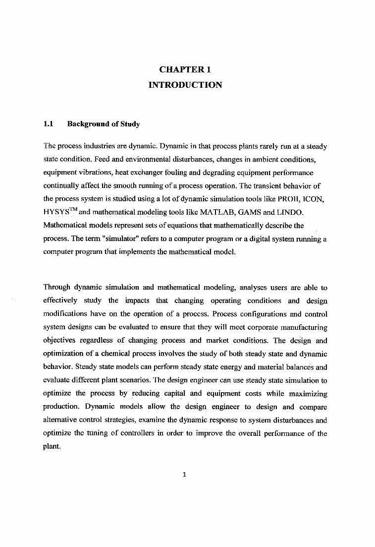
1.1 Background of Study
The process industries are dynamic. Dynamic in that process plants rarely run at a steady
state condition. Feed and environmental disturbances, changes in ambient conditions,
equipment vibrations, heat exchanger fouling and degrading equipment performance
continually affect the smooth running of a process operation. The transient behavior of
the process system is studied using a lot of dynamic simulation tools like PROII, ICON,
HYSYS™and mathematical modeling tools like MATLAB, GAMS andLINDO.
Mathematical models represent sets ofequations that mathematically describe the
process. The term "simulator" refers to a computer program or a digital system running a
computer program that implements the mathematical model.
Through dynamic simulation and mathematical modeling, analyses users are able to
effectively study the impacts that changing operating conditions and design
modifications have on the operation of a process. Process configurations and control
system designs can be evaluated to ensure that they will meet corporate manufacturing
objectives regardless of changing process and market conditions. The design and
optimization of a chemical process involves the study of both steady state and dynamic
behavior. Steady state models can perform steady state energy and material balances and
evaluate different plant scenarios. The design engineer can use steady state simulation to
optimize the process by reducing capital and equipment costs while maximizing
production. Dynamic models allow the design engineer to design and compare
alternative control strategies, examine the dynamic response to system disturbances and
optimize the tuning of controllers in order to improve the overall performance of the
plant.
1.2 Problem Statement
Distillation is the most frequently used separation process. It separates the components
of a mixture on the basis oftheir boiling points and on the difference in the compositions
of the liquids and their vapors.
Certain types ofdistillation columns are designed to produce high purity and ultra purity
products that is product having purity greater than approximately 99.99% by volume.
Such columns are particularly sensitive to the liquid/vapor ratio and can exhibit multiple
steady^state temperature profiles that will rapidly change from one profile to one profile
based on the amount ofvapor rising in the column and the amount of heat introduced
into the column. As a result, during upset condition caused by changed in feed
composition, it can be difficult, to control the liquid vapor ratio within the column and
therefore the product quality.
The product purity of a distillation process is only can be maintained by the
manipulation of the material and energy balances. Difficulties in maintaining that purity
arise because ofdead times, nonlinearities and variable interactions.
1.3 Objectives
The project is mainly about modeling a steady state and dynamic simulation for the high
purity distillation column via MATLAB. Upon completing the project, a few objectives
need to be achieved. The objectives ofthe study are as follows:
i. To study behavior of high purity distillation column at steady state and dynamic
condition.
ii. To develop steady state and dynamic model of high purity distillation column via
MATLAB.
iii. To investigate effect of reflux and reboiler rate disturbance towards top and
bottom product purity.
iv. To obtain the gain and time constant for any changes of column operating
condition through first order process response
1.4 Scope ofWork
The scope of work for the project is to conducta literature review on dynamic behavior
of high purity distillation column. The next step is to proceed with developing
mathematical model of distillation, come out with findings on effect of disturbance
changes towards product purity and also obtaining gain and time constant in order to
develop first order response of top and bottom productwhencolumn operating condition
changes. Through this project student is exposed to explore research problems and build
research objectives, applying appropriate methodology, analyzing and interpreting data
obtained from the mathematical modeling, troubleshooting any predicaments occur and
also reporting the findings.
CHAPTER 2
LITERATURE REVIEW AND THEORY
2.1 Distillation Process
Distillation column is probably the most popular and important process studied in the
chemical engineering literature. Distillation is used in many chemical processes for
separating feed streams and for purification offinal and intermediate product streams.
Most columns handle multicomponent feeds. But many can be approximated by binary
or pseudobinary mixtures.
Distillation can be performed either as a batch or a continuous operation. The main
difference between the two is that in continuous distillation, the feed concentration is
relatively constant, while in batch, the concentration of the light components drops and
that of the heavy components rises as distillation progresses.
Another basic difference between distillation operations is in the handling ofthe heat
removed by the condenser at the top ofthe column. The more common approach is to
waste that heat by rejecting it into the cooling water. In this case, "pay heat" must be
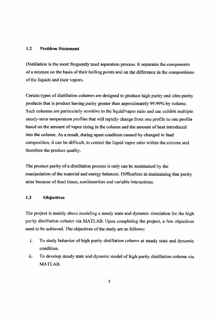
used at the bottom ofthe column in the reboiler. Figure 2.1 illustrates this configuration
and identifies its main components. Because a large part of the total operating cost is in
providing the heat required at the reboiler in some distillation systems, the heat content
of the bottom product is used to preheat the feed to the column.
Condenser
ColumnAccumulator
Feed pumpFtz)
-*D(y>
Reflux pump
Preheater
..^
V,
Reboiler
>BO0
Figure 2.1: Illustration of a tray-type distillation tower, where(without accumulation), the material balance isF = D + BandD = V-L.
The mole fractions of the light key component in the bottoms, distillate and feed are
identified as x, y and z. For binary separation, S = (y[lax])/(x[l-y]).
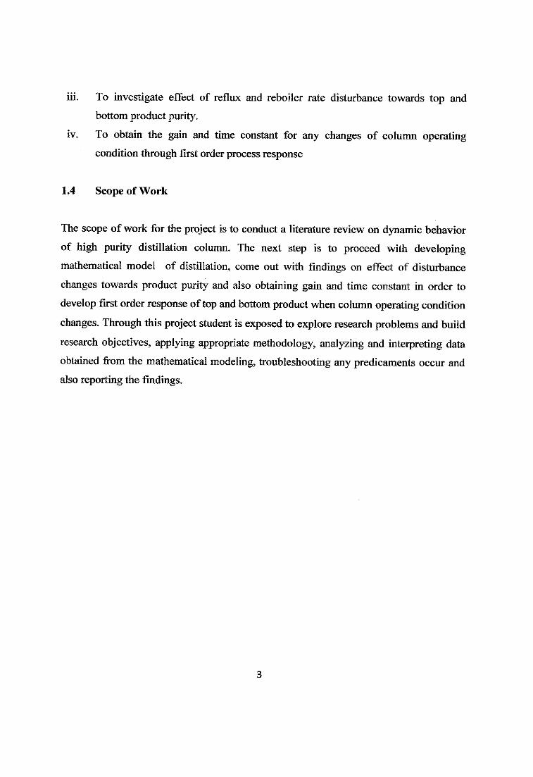
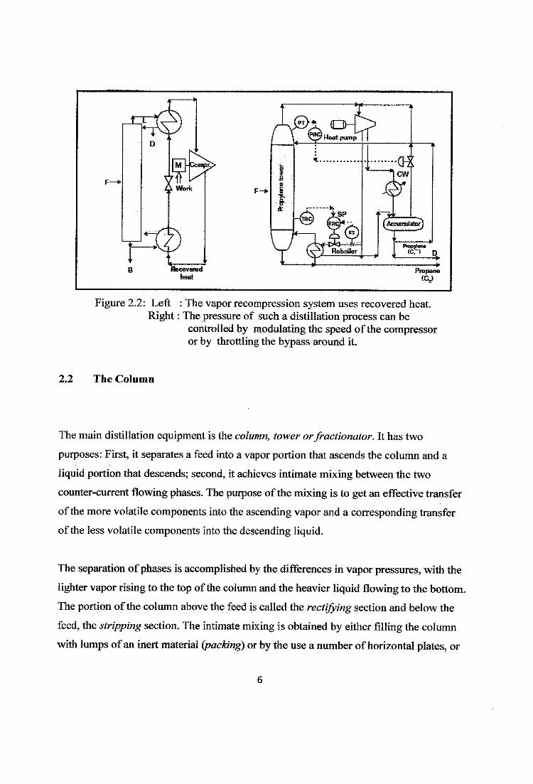
The other option is to recycle the heat removed at the condenser by a heat pump
(compressor). In this configuration, as the vapors from the column (V) are condensed,
the heat from the condenser is used to vaporize a working fluid. These vapors are at the
low pressure of the suction side of the compressor (heat pump). When the working fluid
vapors are compressed, and these high-pressure (and temperature) vapors in the reboiler
contact the bottoms liquid from the column, they condense, and their heat of
condensation serves to vaporize the liquid from the column bottoms (Figure 2.2). While
vapor recompression is energy=efficient, it is not used very frequently.
Work
Recoveredheat
">i OHfe? Heat pump
Figure 2.2: Left : The vapor recompression system uses recovered heat.Right: The pressure of such a distillation process can be
controlled by modulating the speed ofthe compressoror by throttling the bypass around it.
2.2 The Column
The main distillation equipment is the column, tower orfractionator. It has two
purposes: First, it separates a feed into a vapor portion that ascends the column and a
liquid portion that descends; second, it achieves intimate mixing between the two
counter-current flowing phases. The purpose of the mixing is to get an effective transfer
of the more volatile components into the ascending vapor and a corresponding transfer
of the less volatile components into the descending liquid.
The separation ofphases is accomplishedby the differences in vapor pressures, with the
lightervapor rising to the top of the column and the heavier liquid flowingto the bottom.
The portion ofthe column above the feed is called the rectifying section and below the
feed, the stripping section. The intimate mixing is obtained by either filling the column
with lumps of an inertmaterial (packing) or by the use a numberof horizontal plates, or
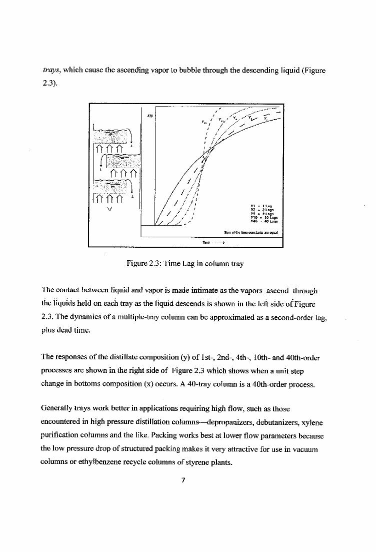
trays, which cause the ascending vapor to bubble through the descending liquid (Figure
2.3).
m
Vt = I LagV2 = 2LagaV4 = 4 LagsMO = 10 LagsV-40 = 40 Lags
Sum oJ the tana constants are equal
Figure 2.3: Time Lag in column tray
The contactbetween liquidand vapor is made intimate as the vapors ascend through
the liquidsheld on each tray as the liquiddescends is shown in the left side ofFigure
2.3. The dynamics of a multiple-tray column can be approximated as a second-order lag,
plus dead time.
The responses of the distillate composition (y) of 1st-, 2nd-, 4th-, 10th- and 40th-order
processes are shown in the right side of Figure2.3 which shows when a unit step
change in bottoms composition (x) occurs. A 40-tray columnis a 40th-orderprocess.
Generally trays work better in applications requiring high flow, such as those
encountered in high pressure distillation columns—depropanizers, debutanizers, xylene
purification columns and the like. Packingworks best at lower flow parameters because
the low pressure drop of structuredpacking makes it very attractive for use in vacuum
columns or ethylbenzene recycle columns of styrene plants.
The influence ofplate efficiency in the operation ofthe distillation tower becomes
important in the control of the overhead composition. Because plate efficiencies increase
with increased vapor velocities, the influence ofthe reflux-to-feed ratio on overhead
composition becomes a nonlinear relationship.
Column dynamics are a function of the number of trays, because the liquid on each tray
must overflow its weir and work its way down the column; therefore, a change in
composition will not be seen at the bottom ofthe tower until some time has passed.
These lags are cumulative as the liquid passes each tray on its way down the column.
Thus, a 30-tray column could be approximated by 30 first-order exponential lags in a
series of approximately the same time constant. The effect of increasing the number of
lags in series is to increase the apparent dead time and increase the response-curve slope.
Thus, the liquid traffic within the distillation process is often approximated by a second^
order lag, plus dead time (Figure 2.3, right).
2.3 Column Variables and Their Pairing
Controlled variables include product compositions, column temperatures and pressure,
and tower and accumulator levels. Manipulatedvariables include reflux, coolant, heating
medium and product flows. Load and disturbance variables include feed-flow rate, feed
composition, steam-header pressure, feed enthalpy, environmental conditions (e.g., rain,
barometric pressure and ambient temperature) and coolant temperature.
The general guidelines for pairing manipulated variables with controlled variables are as
follows:
• Manipulate the stream that has the greatest influence on the controlled variable.
• Manipulate the stream that is more nearly linear with the controlled variable.
• Manipulate the stream that is least sensitive to ambient conditions.
S
• Manipulate the stream least likely to cause interaction.
In a binary distillation process, the number of independent variables is eleven, and the
number ofdefining equations is two. Therefore, the number of degrees of freedom is
nine. Consequently, the maximum theoretical number of automatic controllers that can
be used on a binary distillation process is nine, but usually only five are controlled.
These variables are the compositions ofthe bottom and top products (x and y\ the levels
in the column base and accumulator, and the column pressure. The manipulated
variables that can be assigned to control these are the distillate (£>), bottoms (B) and
reflux (L) flows, the vapor boil-up (Kset by heat input QB), heat removal (QT) and the
ratios ofL/D or V/B. These five
single loops can theoretically be configured in 120 different combinations, and selecting
the right one is a prerequisite to stability and efficiency.
Column pressure almost always is controlled by heat removal (QT). This loop closes the
heat balance around the column, while the levels are controlled to close its material
balance. Therefore, the key task is the assignment of the manipulated variables to the
composition controllers. No matter how we make that selection, these two loops will
interact. A change in one will upset the other because whenever the openings oftheir
control valves change, the material and heat balance of the column will also change.
Therefore, the most important decision in designing the distillation controls is to assign
the least^interacting manipulated variables to the composition control loops. The tool
used in making that selection is the relative gain (RG) calculation.
2.4 Composition Control
Conceptually, product quality is determined by the heat balance ofthe column. The heat
removal determines the internal reflux flow rate, while the heat addition determines the
internal vapor rate. These internal vapor and liquid flow rates determine the circulation
rate, which in turn determines the degree of separation between two key components.
The first task in configuring the control system for a distillation column is to configure
the primary composition control loops. This configuration must consider the interaction
between the proposed control loops, the column's operating objectives and the most
likely disturbance variables. The measurements of the composition control loops can
either be direct or inferred. Table 2.1 provides some guidance on how to select the
manipulated variables for controlling die compositions (and levels) of distillation
columns.
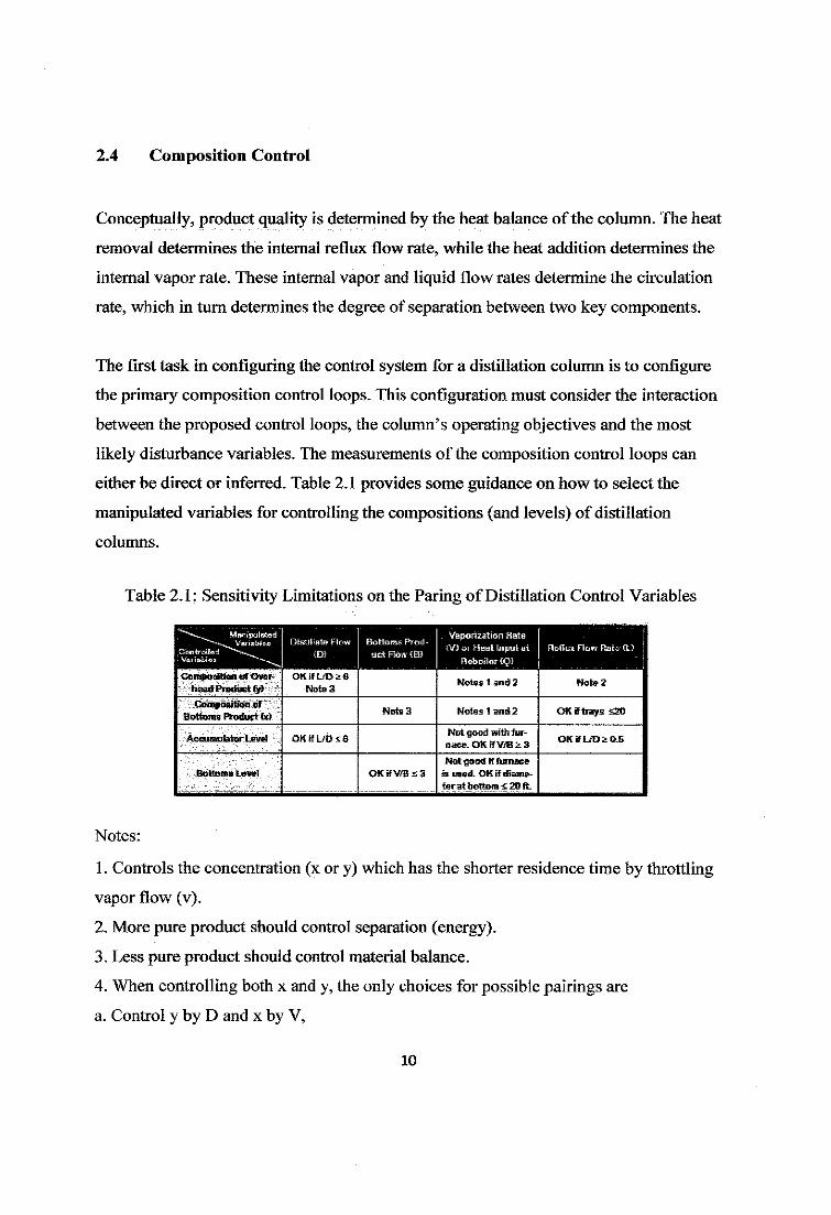
Table 2.1: Sensitivity Limitations on the Paring ofDistillation Control Variables
DtstiSJate Flow Bottoms Prod -
(D) uctRowEBJ
Vaporization Rate
0/5 of KeeS Input at Reflux Bow RaSet QJ
CampoaRian of Over
head Product (y>OKTfLrDsS
Note3Kolas 1 and 2 Mote 2
Composition ofBottoms Product (set
Note 3 Notes 1 and 2 OK if trays s20
Accumulator Level OK if DO 46Not good with fur-na*se.OKHVyBS:3
OKifL/D^aS
Bottoms Level OKifV/Ss;3
Not good iffurnaceis used. OK if diame
ter at bottom s 20 ft.
Notes:
1. Controls the concentration (x or y) which has the shorter residence time by throttling
vapor flow (v).
2. More pure product should control separation (energy).
3. Less pure product should control material balance.
4. When controlling both x and y, the only choices for possible pairings are
a. Control y by D and x by V,
10
b. Control y by D and x by L,
c. Control y by L and x by V,
d. Control y by B and x by L.
Ofthese choices, d is not recommendedbecause a y/B combination is not responsive
dynamically.
2.5 Dynamic Modelling
Dynamic models are used to predict how a process and its controls respond to various
upsets as a function oftime. They can be used to evaluate equipment configurations and
controlschemesand to determine the reliability and safety of a design before capital is
committed to the project. For grassroots and revamp projects, dynamic simulation can be
used to accurately assess transient conditionsthat determine process design temperatures
andpressures. In many cases, unnecessary capitalexpenditures can be avoided using
dynamic simulation.
Dynamic simulation during process design leads to benefits during plant start-up.
Expensive field changes, which impact schedule, can often be minimized if the
equipment and control system is validated using dynamic simulation. Start-up and
shutdown sequences can be tested using dynamic simulation.
Dynamic simulation also provides controller-tuning parameters for use during start-up.
In many cases, accurate controller settings can prevent expensive shutdowns and
accelerate plant start-up. Dynamic simulation models used for process design are not
based on transfer functions as normally found in operator training simulators, but on
fundamental engineeringprinciples and actualphysical equationsgoverningthe process.
When used for process design, dynamic simulation models include:
11
• Equipment models that include mass and energy inventory from
differential balances
• Rigorous thermodynamics based on property correlations, equations of
state, and steam tables
• Actual piping, valve, distillation tray, and equipment hydraulics for
incompressible, compressible, and critical flow
These models are so detailed that the results can influence engineering design decisions
and ensure a realistic prediction of the process and the control system's interaction to
assess control system stability.
12
CHAPTER 3
METHODOLOGY
The design procedure that provides a method ofcontrolling a process comprising the
steps of:
Step 1 Generating a principle steady state and dynamic model
corresponding to the distillation process
Step 2 Simulating the dynamic model for different operating condition
via MATLAB
Step 3 Develop output trend towards changes in input via Pseudo
Random Binary Sequence (PRBS)
Step 4 Develop step response of first order process
Step 5 Obtain the gain and time constant for any changes of column
operating condition through first order process response for
control purposes
3.1 Generating a Principle of Steady State and Dynamic Model Corresponding
to the Distillation Process
In this section is derivation ofa linearizedmodel ofthe plant. Separation of input
components, the feed, is achieved by controlling the transfer ofcomponents between the
various stages (also called trays or plates), within the column,so as to produce output
products at the bottom and at the top of the column.
13
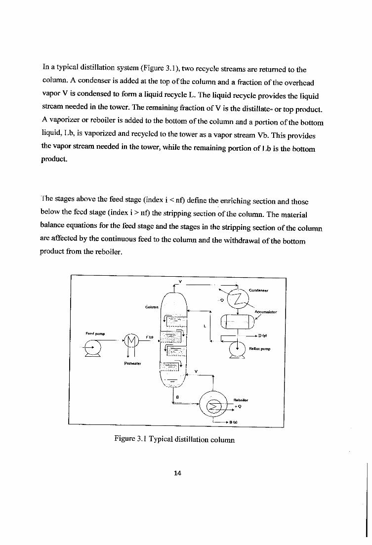
In atypical distillation system (Figure 3.1), tworecycle streams are returned to the
column. A condenser is added at the top of the column and a fraction of the overhead
vapor Vis condensed to form a liquid recycle L. The liquid recycle provides the liquidstream needed in the tower. The remaining fraction ofVisthe distillate- ortop product.Avaporizer or reboiler is added to the bottom ofthe column and aportion ofthe bottomliquid, Lb, is vaporized and recycled to the tower as avapor stream Vb. This providesthe vapor stream needed in the tower, while the remaining portion ofLb is the bottomproduct.
The stages above the feed stage (index i <nt) define the enriching section and thosebelow the feed stage (index i > nf) the stripping section ofthecolumn. The material
balance equations for the feed stage and the stages in the stripping section ofthe columnare affected bythe continuous feed tothe column and thewithdrawal of the bottomproduct from the reboiler.
Feed pump
^F=
W=H
Preheater =Eft
\^r_.y
Condenser
Accumulator
-»-P(y)
+ ) Reflux pump
Reboiler
" + <?
Figure 3.1 Typical distillation column
14
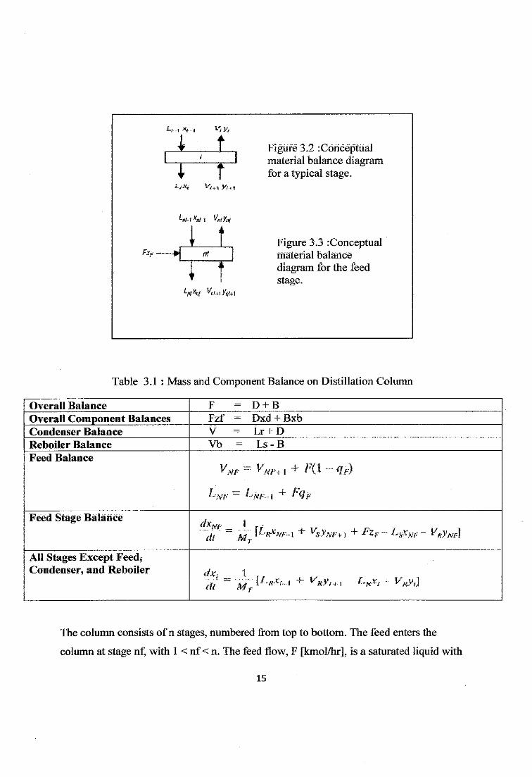
If% * nf
Figure 3.2 Conceptualmaterial balance diagramfor a typical stage.
Figure 3.3 Conceptualmaterial balance
diagram for the feedstage.
Table 3.1 : Mass and Component Balance on Distillation Column
Overall Balance F = D + B
Overall Component Balances Fzf = Dxd + Bxb
Condenser Balance V - Lr + D
Reboiler Balance Vb = Ls - B
Feed Balance
<?/••)
Feed Stage Balance dxm. 1"di' ~ Mr lL**w-i + vsym •*j + ^-" &SXNP ~ ^JVfl
AH Stages Except Feed*Condenser, and Reboiler d*i 1 r ,
J-1 ~~ *-'tfxi '- VmJ
The column consists ofn stages, numbered from top to bottom. The feed enters the
column at stage nf, with 1 < nf< n. The feed flow, F [kmol/hr], is a saturated liquid with
15
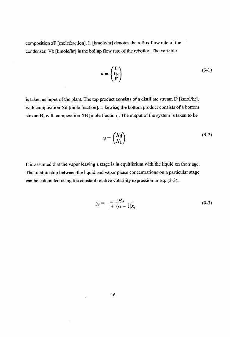
composition zF [molefraction]. L [kmole/hr] denotesthe reflux flow rate ofthe
condenser, Vb [kmole/hr] is the boilup flow rate of the reboiler. The variable
is taken as input of the plant The top product consists of a distillate stream D [kmol/hr],
with composition Xd [mole fraction]. Likewise, the bottom product consists of a bottom
stream B, with composition XB [mole fraction]. The output ofthe system is taken to be
(3-1)
•-(?J
It is assumed that the vapor leaving a stage is in equilibrium with the liquid on the stage.
The relationship between the liquid and vapor phase concentrations on a particular stage
can be calculated using the constant relative volatility expression in Eq. (3-3).
*-i+iiiifc {3-3)
16
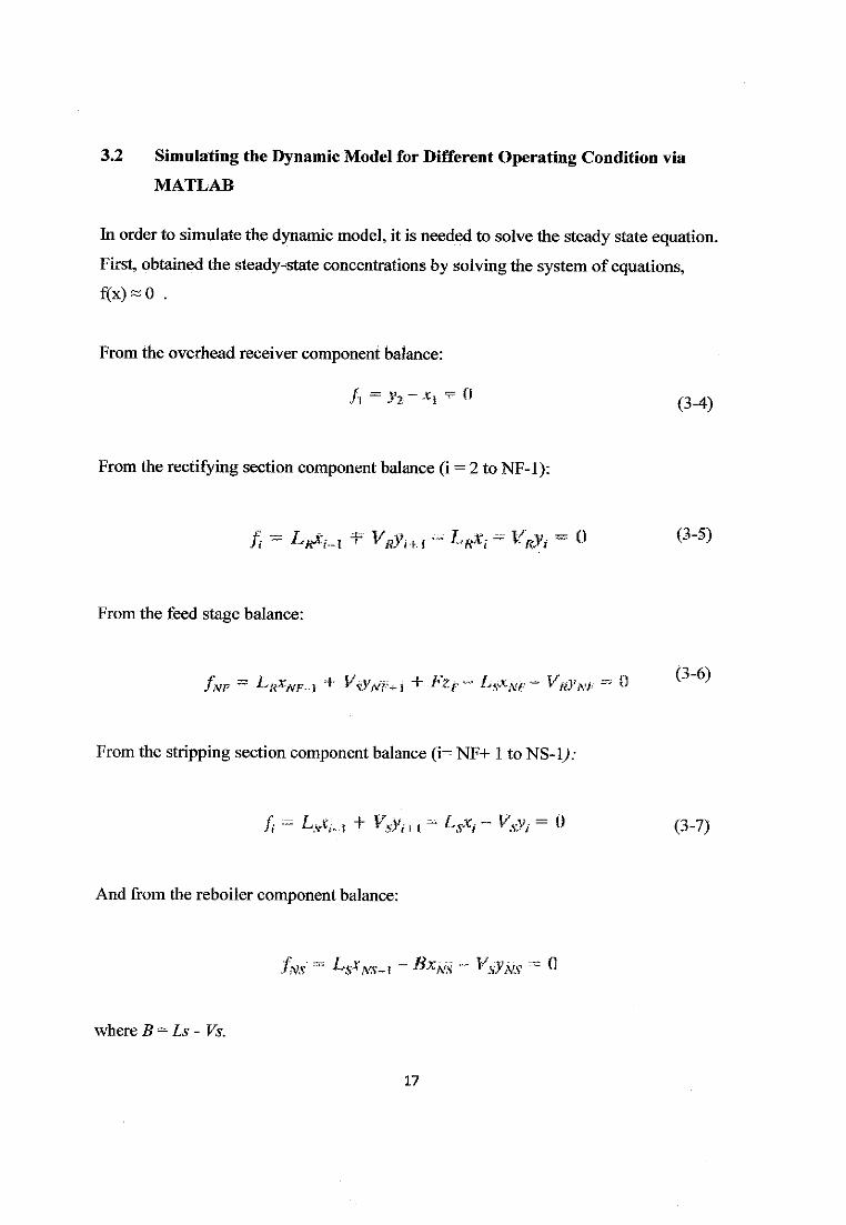
3.2 Simulating the Dynamic Model for Different Operating Condition via
MATLAB
In orderto simulate the dynamic model, it is needed to solve the steady state equation.
First, obtainedthe steady^state concentrations by solving the system of equations,
«x)«0 .
From the overhead receiver component balance:
/i =H-*\ ^ ° (3_4)
From the rectifying section component balance (i = 2 to NF-1):
From the feed stage balance:
From the stripping section componentbalance (i= NF+ 1 to NS-1):
fi = ^-..j + ^ 11 ^ ^,- - Kv>?/ = 0 (3-7)
And from the reboiler component balance:
where B —Ls- Vs.
17
It is realize that the all the equations to solve steady state constitute a set of nonlinear
algebraic equations, since the relative volatility relationship equation is nonlinear in the
state variable.
The equationsarc NS equations in NS unknowns. A Newton-based technique will be
used to solve the equations.
3.3 Output Trend Towards Changes in Input via Pseudo Random Binary
Sequence (PRBS)
By using a simulink, a multiple step change of input can be done by using PRBS.The
purpose is to determinethe trend ofoutputresponsetowards changes in input.
Signal1 I |
Signal Builder Scope
Figure 3.2: Model of input via Simulink
The use ofsignal builder is to createand generate interchangeable groupsof signals
whose waveforms are piecewise linear. Type of signal is set as PRBS with frequency of
10.
18
3.4 Response of First Order Process
First Order Process is use to find how the outlet composition changes when either of the
inputs, reflux(R) or reboiler rate(Vb) is changed. Here is the general first-order transfer
function,
where
Y(s) K.
"'w-tf«- v + 1
Kp : process gain
T : time constant
U(s) : input
Y(s) : output
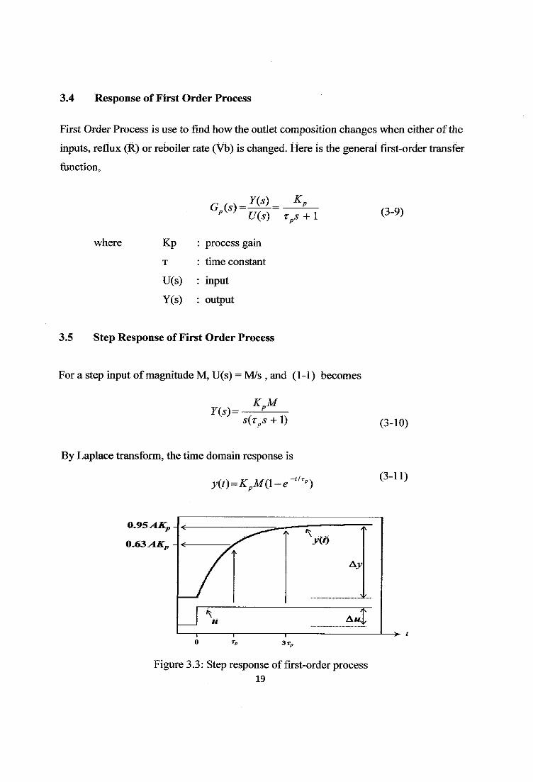
3.5 Step Response of First Order Process
For a step input of magnitude M, U(s) = M/s , and (1-1) becomes
KMY(s)= p
s(ts +1)
By Laplace transform, the time domain response is
0.95AKp 4
0.63 AKP -I
y(t)=KDM(\-e~tlT>)
Figure 3.3: Step response of first-order process19
(3-9)
(3-10)
(3-11)
>~ t
The plot of equation shows that a first-order process does not respond instantaneously to
a sudden change in its input. In fact, after the time interval equal to the process time
constant (t= t), the process response is still only 63.2% complete. Theoretically, the
process output never reaches the new steady state value except as t —•qo; it does
approximate the final steady-state value. Notice that Figure 3.5 has been drawn in
dimensionless or normalized form, with time divided with process time constant and the
output change divided by the product of the process gain and magnitude ofthe input
change.
20
CHAPTER 4
RESULT AND DISCUSSION
4.1 Steady State Operation of a 41-Stage Column
Consider a 41-stage column with the overhead condenser as stage 1, the feed tray as
stage 21and the reboiler as stage 41. The following parameters and inputs apply:
a =1.5
F =1 mol/min
zp = 0.5 mole fraction of light component
R = 2.706 mol/min
D = 0.5 mol/min
qp ~ 1 (sat'd liquid)
From an overall material balance, the bottoms product flowrate is;
B = F~D= 1- 0.5 mol/min
the stripping section flowrate is:
LS = R + FqF = 2.706 + 1 = 3.705 mol/min
and a balance around the reboiler yields:
VS = LS-B = 3.706 - 0.5 = 3.206 mol/min
The m-file dist_ss.m (shown in the Appendix) is used to solve for the steady-state
compositions.
The resulting compositions are shown in Figure 4.1. The sensitivity to reflux rate and
reboiler rate is also shown by the plot in Figure 4.2 and Figure 4.3.21
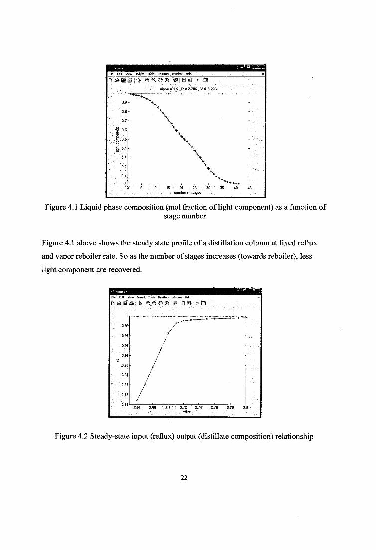
Figure 4.1 Liquid phase composition (mol fraction of light component) as a function ofstage number
Figure 4.1 above shows the steady state profile of a distillation column at fixed reflux
and vapor reboiler rate. So as the number of stages increases (towards reboiler), less
light component are recovered.
Fte EiK Vew Insert Took Dssknp Wiidow Hdp
D^Q#i fe|^<S.^®!«iDSie
Figure 4.2 Steady-state input (reflux) output (distillate composition) relationship
22
From Figure 4.2 above, the steady-state gain (change in output/change in input) for
distillate composition is large when reflux is less than 2.7, but small when the reflux is
greater than 2.71 mol/min.
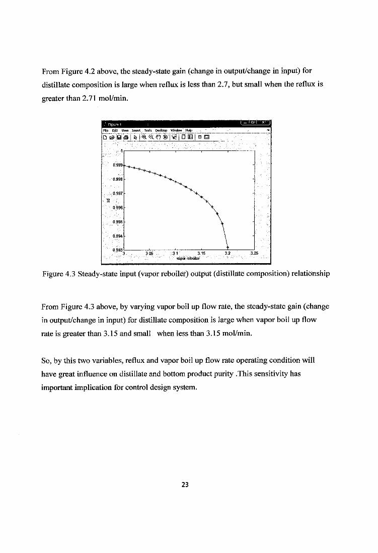
Figure 4.3 Steady-state input (vapor reboiler) output (distillate composition) relationship
From Figure 4.3 above, by varying vapor boil up flow rate, the steady-state gain (change
in output/change in input) for distillate composition is large when vapor boil up flow
rate is greater than 3.15 and small when less than 3.15 mol/min.
So, by this two variables, reflux and vapor boil up flow rate operating condition will
have great influence on distillate and bottom product purity .This sensitivity has
important implication for control design system.
23
4.2 Dynamic Operation of a 41-Stage Column
Consider now the previous problem, with the initial conditions ofthe stage compositions
equal to the steady-state solution. The additional parameters needed for the dynamic
simulation are the molar holdups on each stage. Here we use the following parameters:
Mi = Md =
M5
M3
overhead receiver molar holdup = 5 mol
tray molar holdup = 0.5 mol
hottoms (reboiler) molar holdup = 5 mol
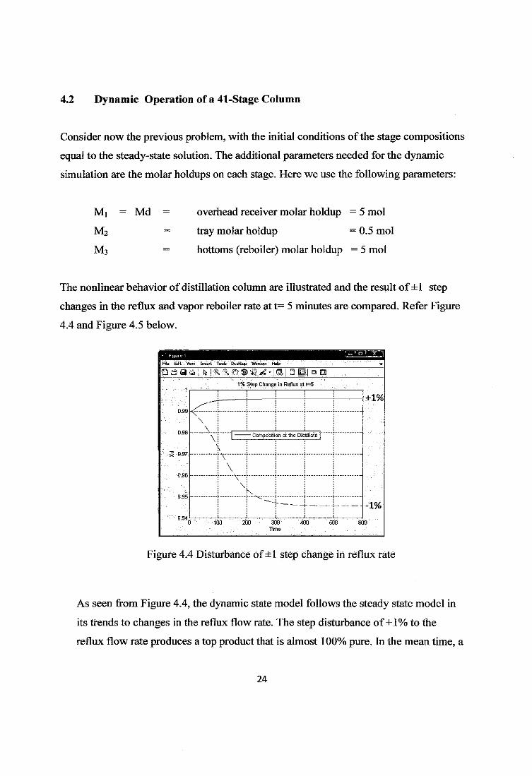
The nonlinear behavior ofdistillation column are illustrated and the result of±1 step
changes in the reflux and vapor reboiler rate at t= 5 minutes are compared. Refer Figure
4.4 and Figure 4.5 below.
osa&i&i-^^os^jMoinisiia
1% Step Change in Reflux at t=5
+1%
_.„Y_.L„.r• Composition at the Distillate •
asr t-\- r i ; t -••\
0.96
KQ.95 - i i—-^<-—; j ;
300
Time
- - -1%
800'
Figure 4.4 Disturbance of ±1 step change in reflux rate
As seen from Figure 4.4, the dynamic state model follows the steady state model in
its trends to changes in the reflux flow rate. The step disturbance of+1% to the
reflux flow rate produces a top product that is almost 100% pure. In the mean time, a
24
-1% step disturbance to the reflux flow rate results in top product being only slightly
above 94% purity.
file eft Wbh Insert Tools Desttop Window
Q6a^|fei^^O®«/-|iiD
0.07
1% Step'.Change in Vapor Reboiler Rate at t=5
1 i0.0S
0.C6
6.04
J '• | Ccmposition atthe Bottom [
0:02
0.01
"^--^ • •-i
-1%
-1%
100 - 200 500 800
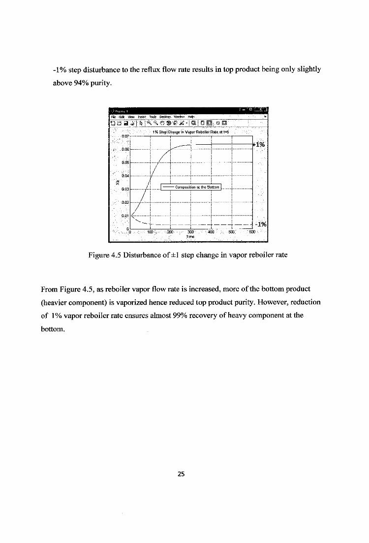
Figure 4.5 Disturbance of±1 step change in vapor reboiler rate
From Figure 4.5, as reboiler vapor flow rate is increased, more of the bottom product
(heavier component) is vaporized hence reduced top product purity. However, reduction
of 1% vapor reboiler rate ensures almost 99% recovery of heavy component at the
bottom.
25
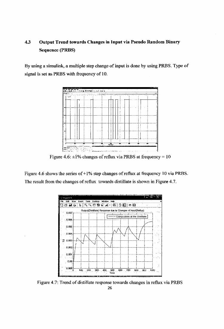
4.3 Output Trend towards Changes in Input via Pseudo Random Binary
Sequence (PRBS)
By using a simulink, a multiple step change of input is done by using PRBS. Type of
signal is set as PRBS with frequency of 10.
£if^5v.~ -f£^^;Vi --..-.+-*,-&- — -'- -" 'la.,< • . .
*..-." 1 j • •-
., __.._ - j - f—- - -f-i
"
-
\
f-I •
|
! !m ™ i
IhvMI
^£LJ
Figure 4.6: ±\% changes of reflux via PRBS at frequency —10
Figure 4.6 shows the series of±1% step changes of reflux at frequency 10 via PRBS.
The result from the changes of reflux towards distillate is shown in Figure 4.7.
Ffe Efft ifiew Insert Toob Desktop Window Help •a
Qaa^i k lE|a D
0.997
0.996
0.995
0.994
-S 0-993
0.992
0.991
0.99
0.389
Qutput(Disii!late) Response due to Changes of inputfJefluit)
: ; : 1 r-innpcsition at theDistillate j
_i\ 4---W-/i"\l-----J|
tiit
100 200 300 40D 500 GOO 700 800 . 900 10Time
00
Figure 4.7: Trend of distillate response towards changes in reflux via PRBS26
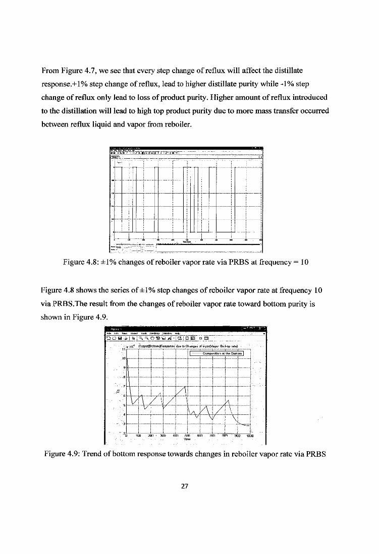
From Figure 4.7, we see that every step change ofreflux will affect the distillate
response.+l% step change of reflux, lead to higher distillate purity while =1% step
change of reflux only lead to loss of product purity. Higher amount of reflux introduced
to the distillation will lead to high top product purity due to more mass transfer occurred
between reflux liquid and vapor from reboiler.
»H >•>•> -...i-J-anSiaiiPHB- " - pp-;1** siIhmH , B
™
-'' |"
— • f —f - j-— - -
|
j!
-
!
!
'.—-•••,—::; :Th*1_q — —
y-1-- •:•'".
Figure 4.8: ±1% changes of reboiler vapor rate via PRBS at frequency = 10
Figure 4.8 shows the series of±1% step changes of reboiler vapor rate at frequency 10
via PRBS.The result from the changes of reboiler vapor rate toward bottom purity is
shown in Figure 4.9.
File Edit Vtow Insoit Tools Deslfop Window htotp
Qcl=B-i! ki^^O^^aS-ISjailin
v tD"3 OtitpuTlBDllomJR&B-pnnsa due IDChanges of inplit(Vapar BoiF-uprate)
1 Composition al the Sottam|- i 1 '. ' '•
3
7
G
5
4
3
O 1DO 200 300 400 EDO 600 700
Time900 1000
Figure 4.9: Trend of bottom response towards changes in reboiler vapor rate via PRBS
27
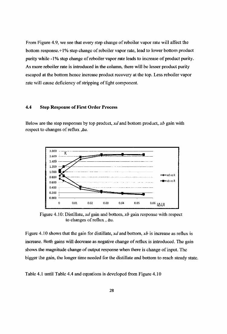
From Figure 4.9, we see that every step change of reboiler vapor rate will affect the
bottom response.+l% step change of reboiler vapor rate, lead to lower bottom product
purity while -1% step change ofreboiler vapor rate leads to increase of product purity.
As more reboiler rate is introduced in the column, there will be lesser product purity
escaped at the bottom hence increase product recovery at the top. Less reboiler vapor
rate will cause deficiency of stripping of light component.
4.4 Step Response of First Order Process
Below are the step responses by top product, xd and bottom product, xb gain withrespect to changes of reflux ,Au.
0.01 0.02 0.03 0.04 0.05 0.06IAUI
•xd vs R
•xb vs R
Figure 4.10: Distillate, xd gain and bottom, xb gain response with respectto changes ofreflux, Au.
Figure 4.10 shows that the gain for distillate, xd and bottom, xb is increase as reflux is
increase. Both gains will decrease as negative change ofreflux is introduced. The gain
shows the magnitude change ofoutput response when there is change ofinput. The
bigger the gain, the longer time needed for the distillate and bottom to reach steady state.
Table 4.1 until Table 4.4 and equations is developed from Figure 4.10
28
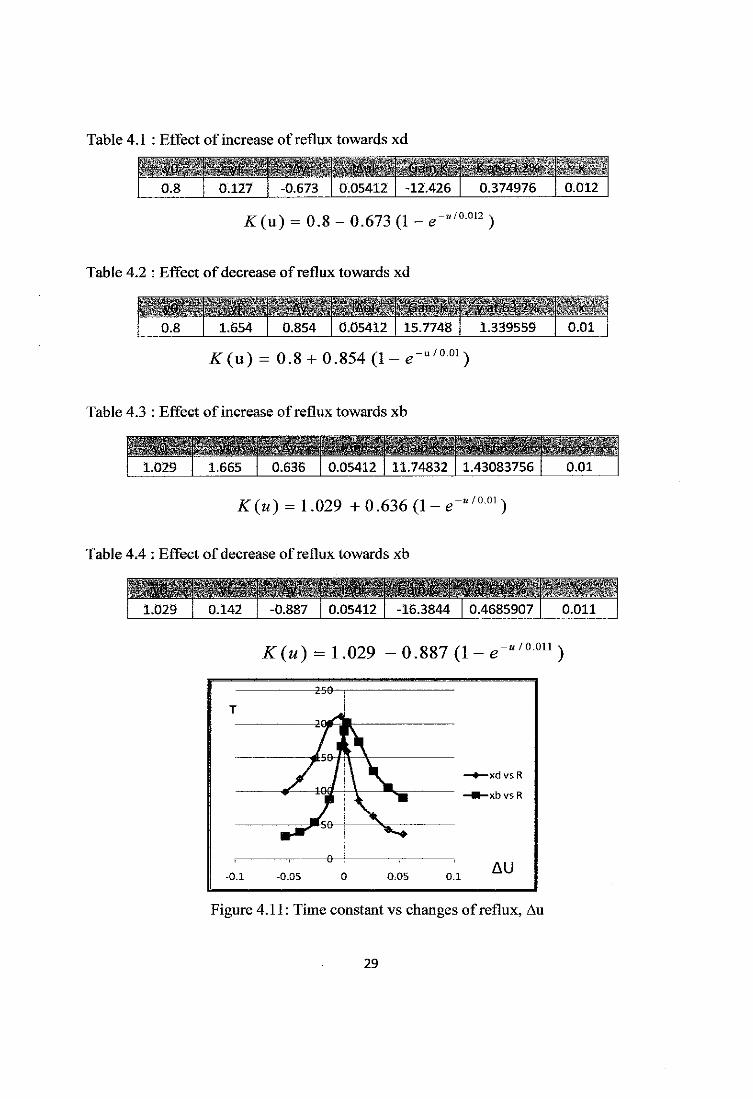
Table 4.1 : Effect of increase of reflux towards xd
0.8 0.127 -0.673 0.05412 -12.426 0.374976 0.012
-w/0.012^(u) = 0.8 - 0.673 (1 - e-'u-u" )
Table 4.2 : Effect of decrease of reflux towards xd
\0 vt Ay lAul Giinfk yfltull''
, l.UJ. , U.^51 , 0.0b 112 , l..//1b , l.^lbS , C.Q1 ,
-u/0.01K(u) = 0.8 + 0.854 (l-e~u/um)
Table A3 : Effect of increase of reflux towards xb
1.029 1.665 0.636 0.05412 11.74832 1.43083756 0.01
-uf 0.01K(u) = 1.029 + 0.636 (l-e"/uul)
Table 4t4 : Effect of decrease of reflux towards xb
vo vt Ay iAuf Gam K > -H € -I •> ' X
1.029 0.142 -0.887 0.05412 -16.3844 0.4685907 0.011
-u/0.011K(u) = 1.029 - 0.887 (l-e"/UU11)
-250-
-0.1 -0.05 0 0.05 0.1
•xd vs R
•xbvsR
AU
Figure 4.11: Time constant vs changes of reflux, Au
29
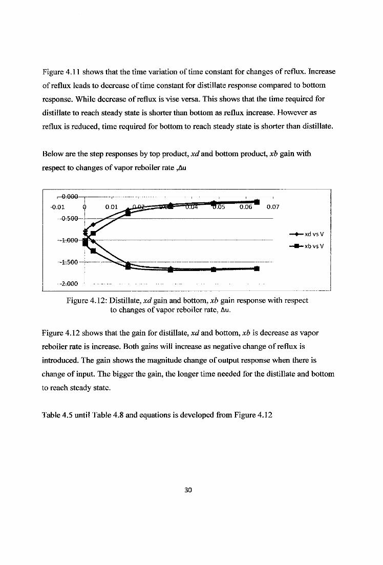
Figure 4.11 shows that the time variation of time constant for changes of reflux. Increase
of reflux leads to decrease of time constant for distillate response compared to bottom
response. While decrease ofreflux is vise versa. This shows that the time required for
distillate to reach steady state is shorter than bottom as reflux increase. However as
reflux is reduced, time required for bottom to reach steady state is shorter than distillate.
Below are the step responses by top product, xd and bottom product, xb gain with
respect to changes ofvapor reboiler rate ,Au
r-ooea—, •—i—• ~i—
^1
0.01 (j o.oi^jwg^ssasA u.u4 ' %.05 ~~0"06 ™ o.c
—1t090H
-h5Q0
-2:000
•xd vs v
•xbvs V
Figure 4.12: Distillate, xt/gain and bottom, xb gain response with respectto changes ofvapor reboiler rate, Au.
Figure 4.12 shows that the gain for distillate, xdand bottom, xb is decrease as vapor
reboiler rate is increase. Both gains will increase as negative change of reflux is
introduced. The gain shows the magnitude change of output response when there is
change of input. The bigger the gain, the longer time needed for the distillate and bottom
to reach steady state.
Table 4.5 until Table 4.8 and equations is developed from Figure 4.12
30
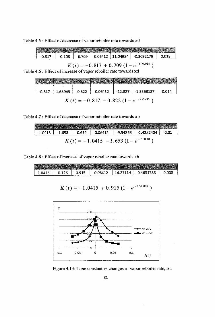
Table 4*5 : EffeGt of decrease ofvapor reboiler rate towards xd
yd \F A* IAiji (jihi\ y il W 7 t
-0.817 I -0.108 I 0.709 I 0.06412 I 11.04984 I -0.3692179 I 0.018
K(t) = -0.817 + 0.709 (1 - e"0018 )Table 4.6 : Effect of increase ofvapor reboiler rate towards xd
-0.817 1.63949 -0.822 0.06412 -12.827 -1.3368127 0.014
-//0.014K(t) = -0.817 - 0.822 (1 - e-uvm* )
Table 4,7 : Etfect of decrease ofvapor reboiler rate towards xb
-t/O.OlK(t) = -l.04\5 -1.653 (l-*r'/UUI)
Table 4,8 : EffeGt of increase ofvapor reboiler rate towards xb
-1 0415 -0126 0 915 0 06412 14 27114 j -0 4631788 0 008
-f/0.008K(t) = -l.04l5 + 0.915 (l-e-"UUUK)
-2-50
-0-4
-0.1 -0.05 0.05 O.l
-XdvsV
•XbvsVb
AU
Figure 4.13: Time constant vs changes of vapor reboiler rate^ Au
31
Figure 4.13 shows that the time variation of time constant for changes of vapor reboiler
rate. Increase ofvapor reboiler rate leads to decrease of time constant for bottom
response compared to distillate response. While decrease of vapor reboiler rate is vise
versa. This shows that the time required for bottom to reach steady state is shorter than
distillate as vapor reboiler increase. However as vapor reboiler is reduced, time required
for distillate to reach steady state is shorter than the bottom.
32
CHAPTER 5
CONCLUSION AND RECOMMENDATION
After discussing the results of the simulations for both dynamic and steady state
distillation column, it can be concluded that the objective of this project is achieved as
the MATLAB models represent an ideal distillation column..The assumptions made for
this project was fairly rigid and elementary. To obtain more accurate results from the
simulations, the assumptions need to include:
• energy balance
• complex tray hold up
• lag time or dead time
This will ensure the model would mimic an actual behavior of distillation column.
Below are the several recommendations suggested in order to be able to pursue project
further.
1. To incorporate energy balances into the mathematical model
2. To incorporate lag and dead time.
3. To incorporate the Francis Weir tray hydraulic in order to study the variation
ofvapor and liquid holdup
4. To incorporate a multicomponent mixture of components into the model.
33
REFERENCES
Books/Jouina Is
[1] D.E. Seborg, T.F. Edgar and D.A. Mellichamp, Process dynamics and control
(2nd ed.), John Wiley & Sons, New York, USA (2004)
[2] Robin Smith. 2005,"Chemical Process Design and Heat Integration", University
of Manchester, Wiley
[3] C. R. Cutler and B. L. Ramaker. "DynamicMatrix Control-A Computer
Control Algorithm," Paper No. 51b, AJChe 86th National Meeting, April 1979.
[4] Bela G. Liptak (1995), Instrument Engineers' Handbook: Process Control.
[5] C. E. Garcia and M. Morari.24 (1985), "Internal Model Control 3 - Multivariable
Control Law Computation and Tuning Guidelines," Ind. Eng. Chem. Process
Des. Dev: 484-94.
[6] Nur Rasyeda bt Mohd Raziff (2004) /'Control ofReactive Distillation Column",
Universiti Teknologi PETRONAS (UTP), Perak
Websites
1. http://www. cheresources.com/invision/lofiversion/index.php/t5568.html
2. http://www.aspentech.com/publication_files/Distillation_Column_Control_Desig
n_Using_Steady_State.pdf
34
APPENDIX
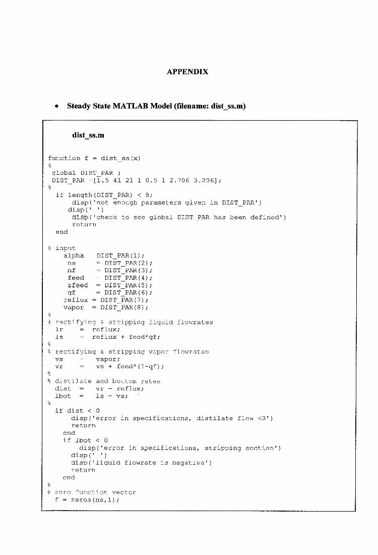
Steady State MATLAB Model (filename: dist_ss.m)
dist ss.m
function f = dist_ss(x)
global DIST_PAR ;DIST^PAR =[1.5 41 21 1 0.5 1 2.706 3.206];
if length(DIST_PAR) < 8;disp('not enough parameters given in DIST_PAR')
disp(' ')
disp('check to see global DIST_PAR has been defined'}return
end
% input
alpha =DIST_PAR(1) ;tis = DIST_PAR(2) ;nf = DIST_PAR(3);feed = DIST_PAR(4) ;zfeed = DIST_PAR(5);qf = DIST_PAR(6} ;
reflux = DIST_PAR{7};vapor = DIST_PAR(8);
% rectifying & stripping liquid flowrateslr = reflux;
Is = reflux + feed*qf;
"5
% rectifying & stripping vapor flowrates
vs = vapor;
vr = vs + feed*(1-qf);
% distilate and bottom rates
dist = vr - reflux;
lbot = Is - vs;
if dist < 0
disp('error in specifications, distilate flow <0')return
end
if lbot < 0
disp('error in specifications, stripping section')disp (' ')disp('liquid flowrate is negative')return
end
% zero function vector
f = zeros(ns, 1);
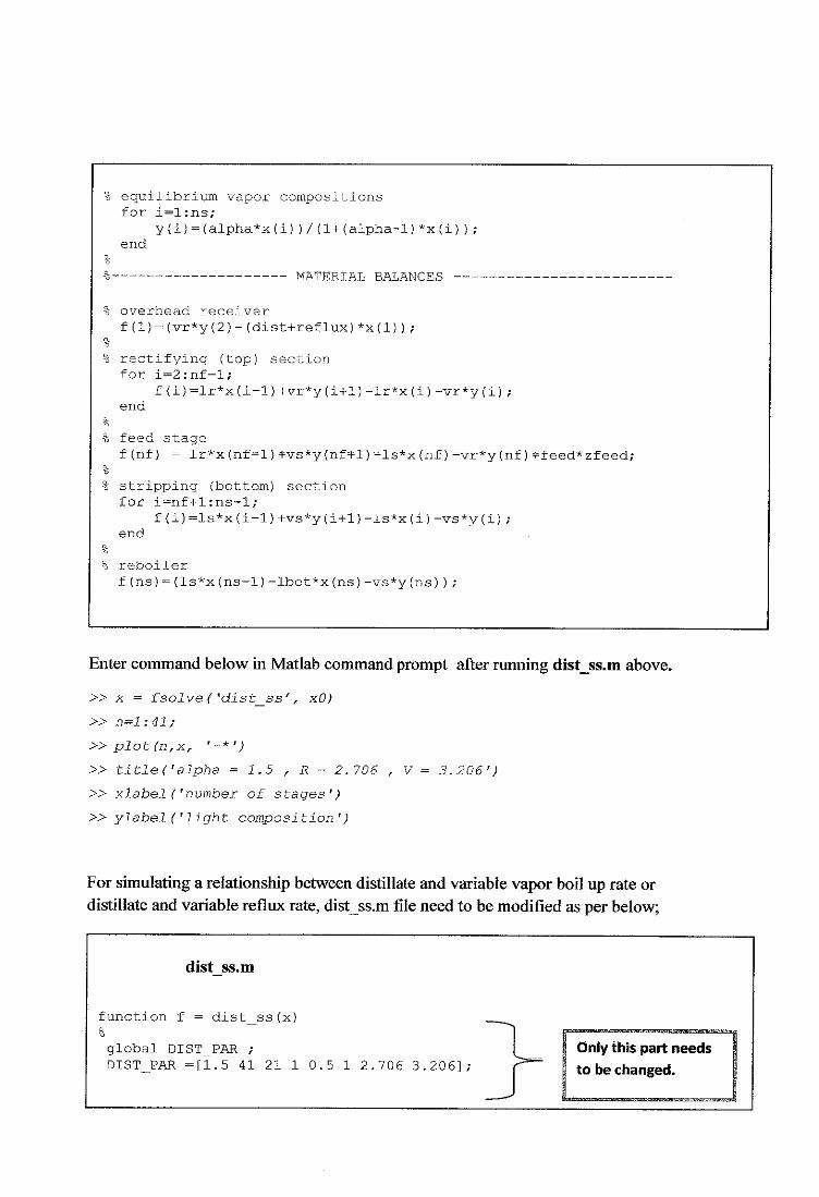
% equilibrium vapor compositionsfor i=l:ns;
y(i)=(alpha*x(i) )/ (l+(alpha-l) *x(i));end
% MATERIAL BALANCES
% overhead receiver
f(l)=(vr*y(2)-(dist+reflux)*x(l));
% rectifying (top) section
for i=2:nf-l;
f{i)=lr*x(i-l)+vr*y(i+l)-lr*x(i)-vr*y(i);end
% feed stage
f(nf) = lr*x(nf-l)+vs*y(nf*l)-ls*x(nf) -vr*y(nf)*feed*zfeed;
% stripping (bottom) sectionfor i=nf+1:ns-1;
f(i)=ls*x(i-l)+vs*y(i+l)-ls*x(i) -vs*y(i);end
% reboiler
f(ns)=(ls*x(ns-l)-lbot*x(ns)-vs*y (ns) );
Enter command below in Matlab command prompt after running dist_ss.m above.
» x = fsolve ( *dist_ss', xO)
» n=l:41;
» plot (n,K, '-*')
» title ('alpha = 1.5 , R = 2. 106 , V = 3.206')
» xlabel ('number of stages')
» ylabel ('light composition')
For simulating a relationship between distillate and variable vapor boil up rate ordistillate and variable reflux rate, distss.m tile need to be modified as per below;
distss.m
function f = dist_ss(x)
global DIST PAR ; Only this part needsdist^par =[1.5 41 21 l 0.5 1 2.706 3.206]; r^~ j to be changed.
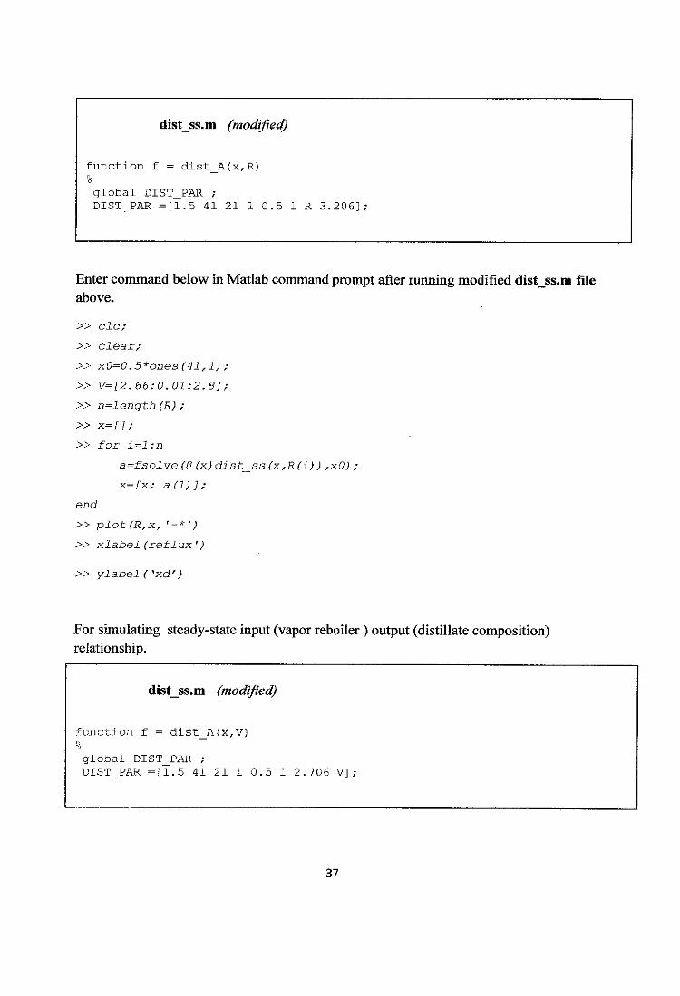
distss.m (modified)
function f = dist_A(x,R)
global DIST_PAR ;DIST PAR =[1.5 41 21 1 0.5 1 R 3.206];
Enter command below in Matlab command prompt after running modified dist_ss.m fileabove.
» clc;
» clear;
» x0=0.5*ones(41,1) ;
» V=12. 66:0.01:2.8];
» n=length (R);
» x=[];
» for i=l:n
a-fsolve (@ (x) dist_ss (x,R (i) ) fx0) ;
x=[x; a (1) ] ;
end
» plot (R,xr '-*')
» xlabel (reflux')
» ylabel ( 'xd')
For simulating steady-state input (vapor reboiler ) output (distillate composition)relationship.
dist_ss.m (modified)
function f = dist_Mx V)
global DIST PAR ;
DIST_PAR =[1.5 41 21 1 0.5 1 2 706 V];
37
Enter command below in Matlab command prompt in after running modified dist_ss.mfile above.
» clc;
» clear;
» x0=0.5*ones(4l,l) ;
» V=[3:0.01:3.206];
» n=length (V) ;
» x=[J;
» for 1=1:n
a~fsolve (@ (x) dist_ss (xrV(i) ) fx0) ;
x=[x; a (1) ] ;
end
» plot(V/x/ '-*')
» xlabel('vapor reboiler')
» ylabel ( *xd')
Dynamic MATLAB Model (filename: distdyn.m)
function xdot = dist_dyn(t,x);global DIST PAR
%input
alpha = DIST PAR(1);
ns = dist]_PAR{2);nf = DIST PAR(3);
feed! = DIST _PAR (4);zfeedi = DIST PAR(5) ;
qf = dist]_PAR (6) ;
refluxi = DIST_ PAR (7 ) ;
vapori = DIST PAR(8);
md = DIST PAR (9) ;
mb = DIST_ PAR(10);
mt = DIST _PAR(11);
if length(DIST PAR) ==
stepr = DIST _PAR(12) ;tstepr = DIST.. ..PAR(13) ;
stepv = DIST_J?AR{14) ;tstepv = DIST PAR(15);
stepzf = DIST PAR(16) ;
relative volatilitytotal number of stages
feed stage
initial feed flowrate
initial feed composition, lightfeed quality (1 = sat'd liqd,
0 = sat'd vapor) (1)initial reflux flowrate
initial reboiler vapor flowrate
distillate molar hold-upbottoms molar hold-up
stage molar hold-up
magnitude step in refluxtime of reflux step changemagnitude step in vaportime of vapor step changemagnitude of feed comp change
38
comp
tstepzf = DIST_PAR(17)Stepf = DIST_PAR(i8)tstepf = DIST_PAR(19)else
% time of feed comp change
% magnitude of feed flow change% time of feed flow change
stepr =0; tstepr = 0; stepv = 0; tstepv = 0;stepzf = 0; tstepzf = 0; stepf = 0; tstepf = 0;end
if t < tstepr;reflux = refIuxi;
else
reflux = refluxi + stepr;end
if t < tstepv;vapor = vapori;else
vapor = vapori + stepv;end
if t < tstepzf;zfeed = zfeedi;
else
zfeed = zfeedi + stepzf;end
if t < tstepf;feed = feedi;
else
feed = feedi + stepf;end
% rectifying and stripping section liquid flowrateslr = reflux;
ls = reflux + feed*qf;
% rectifying and stripping section vapor flowrates
vs = vapor;
vr = vs + feed*(1-qf} ;
% distillate and bottoms rates
dist = vr - reflux;
lbot = Is - vs;
% zero the function vector
xdot = zeros(ns,l);
% calculate the equilibrium vapor compositionsfor i=l:ns;
y(i)=(alpha*x(i))/(1.+(alpha-1.)*x(i));end
39
MATERIAL BALANCES
% overhead receiver
xdot(l)=(l/md)*{vr*y(2)-(dist+reflux)*x{l));
% rectifying (top) sectionfor i=2:nf-l;
xdot(i)=(l/mt)*(lr*x(i-l)+vr*y(i+l)-lr*x(i)-vr*y{i));end
% feed stage
xdot(nf) = (l/mt)*(lr*x(nf-l)+vs*y(nf+l)-ls*x(nf)~vr*y(nf)+feed*zfeed);
% stripping (bottom) sectionfor i=nf+l:ns-l;
xdot(i)=(l/mt)*(ls*x(i-l)+vs*y(i+l)-ls*x(i)-vs*y(i));end
% reboiler
xdot(ns)= (l/mb)*(ls*x(ns-1)-lbot*x(ns)-vs*y(ns));
Dynamic State Calling File(filename: Rlp.m)
%+5% step change of refluxclc;
clear;
global DiST_PARDIST_PAR(1)=1.5; % relative volatility (1.5)
DIST_PAR(2)=41 % total number of stages (41)DIST_PAR(3)-21 % feed stage (21)
DIST_PAR(4)=1 % initial feed flowrate (1)DIST_PAR(5)=0.5 % initial feed composition, light comp (0.5)DIST_PAR(6)=1 % feed quality (1 = sat'd liqd,
% 0 = sat'd vapor) (1)DIST_PAR(7)=2.706 % initial reflux flowrate (2.706)DIST_PAR(8)=3i206 % initial reboiler vapor flowrate (3.206)DIST_PAR(9)=5 % distillate molar hold-up (5)DIST_PAK(1Q)=5 % bottoms molar hold-up (5)
DIST_PAR(11)=0.5 % stage molar hold-up (0.5)
DIST_PAR(12)=0.02706;DIST PAR(13)=5;
DIST~PAR(14)=0;DIST_PAR(15)=0,DIST_PAR(i6j=0,DIST_PAR(17)=0,DIST_J>AR{18)=0,DIST PAR(19)=0.
40
x0=0.5*ones(41,l);n=ones(41:1);
n=[l:41]';
for i=l:n
xO=fsolve('dist_ss',xO);end
[t,x]=ode45('dist_dyn',[0:1:600],x0);plot(t,x(:,1)),xlabel('Time'),ylabel('Xd') ,legend('Composition at theDistillate',0)
hold on
DIST_PAR(12)=-0.02706;[t,x]=ode45('dist_dyn',[0:1:600],x0) ;plot(t,x(:,l), 'r—')grid on
title('1% Step Change in Reflux at t=5' )
41