18
Automatization of Decision Processes in Conflict Situations: Modelling,
Simulation and Optimization
Zbigniew Tarapata Military University of Technology in Warsaw, Faculty of Cybernetics
Poland
1. Introduction
Military conflict is one of the types of conflict situations. The automation of simulated battlefield is a domain of Computer Generated Forces (CGF) systems or semi-automated forces (SAF or SAFOR) (Henninger et al., 2000; Lee & Fishwick, 1995; Longtin & Megherbi, 1995; Lee, 1996; Mohn, 1994; Petty, 1995). CGF or SAF (SAFOR) is a technique, which provides a simulated opponent using a computer system that generates and controls multiple simulation entities using software and possibly a human operator. In the case of Distributed Interactive Simulation (DIS) systems, the system is intended to provide a simulated battlefield which is used for training military personnel. The advantages of CGF are well-known (Petty, 1995): they lower the cost of a DIS system by reducing the number of standard simulators that must be purchased and maintained; CGF can be programmed, in theory, to behave according to the tactical doctrine of any desired opposing force, and so eliminate the need to train and retrain human operators to behave like the current enemy; CGF can be easier to control by a single person than an opposing force made up of many human operators and it may give the training instructor greater control over the training experience. One of the elements of the CGF systems is module for movement planning and simulation of military objects. In many of existing simulation systems there are different solutions regarding to this subject. In the JTLS system (JTLS, 1988) terrain is represented using hexagons with sizes ranging from 1km to 16km. In the CBS system (Corps Battle Simulation, 2001) terrain is similarly represented, but vectoral-region approach is additionally applied. In both of these systems there are manual and automatic methods for route planning (e.g. in the CBS controller sets intermediate points (coordinates) for route). In the ModSAF (Modular Semi-Automated Forces) system in module “SAFsim”, which simulates the entities, units, and environmental processes the route planning component is located (Longtin & Megherbi, 1995). In the paper (Mohn, 1994) implementation of a Tactical Mission Planner for command and control of Computer Generated Forces in ModSAF is presented. In the work (Benton et al., 1995) authors describe a combined on-road/off-road planning system that was closely integrated with a geographic information system and a simulation system. Routes can be planned for either single columns or multiple columns. For multiple columns, the planner keeps track of the temporal location of each column and insures they will not occupy the same space at the same time. In the same paper the Hierarchic Route
www.intechopen.com
Automation and Robotics
298
Planner as integrate part of Predictive Intelligence Military Tactical Analysis System (PIMTAS) is discussed. In the paper (James et al., 1999) authors presented on-going efforts to develop a prototype for ground operations planning, the Route Planning Uncertainty Manager (RPLUM) tool kit. They are applying uncertainty management to terrain analysis and route planning since this activity supports the Commander’s scheme of manoeuvre from the highest command level down to the level of each combat vehicle in every subordinate command. They extend the PIMTAS route planning software to accommodate results of reasoning about multiple categories of uncertainty. Authors of the paper (Campbell et al., 1995) presented route planning in the Close Combat Tactical Trainer (CCTT). Authors (Kreitzberg et al., 1990) have developed the Tactical Movement Analyzer (TMA). The system uses a combination of digitized maps, satellite images, vehicle type and weather data to compute the traversal time across a grid cell. TMA can compute optimum paths that combine both on-road and off-road mobility, and with weather conditions used to modify the grid cost factors. The smallest grid size used is approximately 0.5 km. The author uses the concept of a signal propagating from the starting point and uses the traversal time at each cell in the array to determine the time at which the signal arrives to neighbouring cells. In the paper (Tarapata, 2004a) models and methods of movement planning and simulation in some simulation aided system for operational training on the corps-brigade level (Najgebauer, 2004) is described. A combined on-road/off-road planning system that is closely integrated with a geographic information system and a simulation system is considered. A dual model of the terrain ((1) as a regular network of terrain squares with square size 200mx200m, (2) as a road-railroad network), which is based at the digital map, is presented. Regardless of types of military actions military objects are moved according to some group (arrangement of units). For example, each object being moved in group (e.g. during attack, during redeployment) must keep distances between each other of the group (Tarapata, 2001). Therefore, it is important to recognize (during movement simulation) that objects inside units do not “keep” required distances (group pattern) and determine a new movement schedule. All of the systems presented above have no automatic procedures for synchronization movement of more than one unit. The common solution of this problem is when movement (and simulation, naturally) is stopped and commanders (trainees) make a new decision or the system does not react to such a situation. Therefore, in the paper (Tarapata, 2005) a proposition of a solution to the problem of synchronization movement of many units is shown. Some models of synchronous movement and the idea of module for movement synchronization are presented. In the papers (Antkiewicz et al., 2007; Tarapata, 2007c) the idea and model of command and control process applied for the decision automata on the battalion level for three types of unit tasks: attack, defence and march are presented. The chapter is organized as follows. Presented in section 2 is the review of methods of environment modelling for simulated battlefield. An example of terrain model being used in the real simulator is described. Moreover, paths planning algorithms, which are being applied in terrain-based simulation, are considered. Sections 3 and 4 contain description of automatization methods of main battlefield processes (attack, defence and march) in simulation system like CGF. In these sections, a decision automata, which is a component of the simulation system for military training is described as an example. Presented in section 5 are some conclusions concerning problems and proposition of their solution in automatization of decision processes in conflict situations.
www.intechopen.com

Automatization of Decision Processes in Conflict Situations: Modelling, Simulation and Optimization
299
2. Environment modelling for simulation of conflict situations
2.1 An overview
The terrain database-based model is being used as an integrated part of route CGF systems.
Terrain data can be as simple as an array of elevations (which provides only a limited means
to estimate mobility) or as complex as an elevation array combined with digital map
overlays of slope, soil, vegetation, drainage, obstacles, transportation (roads, etc.) and the
quantity of recent weather. For example, in (Benton et al., 1995) authors describe HERMES
(Heterogeneous Reasoning and Mediator Environment System) will allow the answering of
queries that require the interrogation of multiple databases in order to determine the start
and destination parameters for the route planner.
There are a few approaches in which the map (representing a terrain area) is decomposed
into a graph. All of them first convert the map into regions of go (open) and no-go (closed).
The no-go areas may include obstacles and are represented as polygons. A few methods of
map representation is used, for example: visibility diagram, Voronoi diagram, straight-line
dual of the Voronoi diagram, edge-dual graph, line-thinned skeleton, regular grid of
squares, grid of homogeneous squares coded in a quadtree system, etc. (Benton et al., 1995;
Schiavone et al., 1995a; Schiavone et al., 1995b; Tarapata, 2003).
The polygonal representations of the terrain are often created in database generated systems
(DBGS) through a combination of automated and manual processes (Schiavone et al., 1995;
Schiavone et al., 2000). It is important to say that these processes are computationally
complicated, but are conducted before simulation (during preparation process). Typically,
an initial polygonal representation is created from the digital terrain elevation data through
the use of an automated triangulation algorithm, resulting in what is commonly referred to
as a Triangulated Irregular Network (TIN). A commonly used triangulation algorithm is the
Delaunay triangulation. Definition of the Delaunay triangulation may be done via its direct
relation to the Voronoi diagram of set S with an N number of 2D points: the straight-line
dual of the Voronoi diagram is a triangulation of S.
The Voronoi diagram is the solution to the following problem: given set S with an N number
of points in the plane, for each point pi in S what is the locus of points (x,y) in the plane that
are closer to pi than to any other point of S?
The straight-line dual is defined as the graph embedded in the plane obtained by adding a
straight-line segment between each pair of points of S whose Voronoi polygons share an
edge. Fig.1a depicts an irregularly spaced set of points S, its Voronoi diagram, and its
straight-line dual (i.e. its Delaunay triangulation).
The edge-dual graph is essentially an adjacency list representing the spatial structure of the
map. To create this graph, we assign a node to the midpoint of each map edge, which does
not bound an obstacle (or the border). Special nodes are assigned to the start and goal
points. In each non-obstacle region, we add arcs to connect all nodes at the midpoints of the
edges, which bound the same region. The fact that all regions are convex, guarantees that all
such arcs cannot intersect obstacles or other regions. An example of the edge-dual graph is
presented in Fig.1b.
The visibility graph, is a graph, whose nodes are the vertices of terrain polygons and edges
join pairs of nodes, for which the corresponding segment lies inside a polygon. An example
is shown in Fig.2.
www.intechopen.com

Automation and Robotics
300
(a) (b)
Fig.1. (a) Voronoi diagram and its Delaunay triangulation (Schiavone et al., 1995); (b) Edge-dual graph. Obstacles are represented by filled polygons
Fig.2. Visibility graph (Mitchell, 1999). The shortest geometric path is marked from source node s to destination t. Obstacles are represented by filled polygons
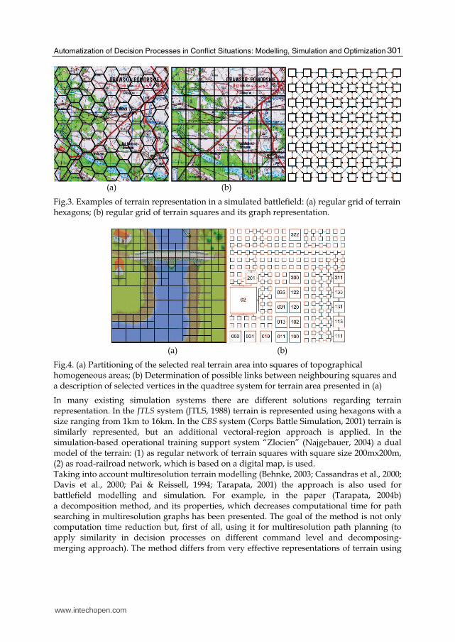
The regular grid of squares (or hexagons, e.g. in JTLS system (JTLS, 1988)) divides terrain
space into the squares with the same size and each square is treated as having homogeneity
from the point of view of terrain characteristics (Fig.3).
The grid of homogeneous squares coded in quadtree system divides terrain space into the squares
with heterogeneous size (Fig.4). The size of square results from its homogeneity according to
terrain characteristics. An example of this approach was presented in (Tarapata, 2000).
Advantages and disadvantages of terrain representations and their usage for terrain-based
movement planning are presented in section 2.3.
www.intechopen.com
Automatization of Decision Processes in Conflict Situations: Modelling, Simulation and Optimization
301
(a) (b)
Fig.3. Examples of terrain representation in a simulated battlefield: (a) regular grid of terrain hexagons; (b) regular grid of terrain squares and its graph representation.
(a) (b)
Fig.4. (a) Partitioning of the selected real terrain area into squares of topographical homogeneous areas; (b) Determination of possible links between neighbouring squares and a description of selected vertices in the quadtree system for terrain area presented in (a)
In many existing simulation systems there are different solutions regarding terrain representation. In the JTLS system (JTLS, 1988) terrain is represented using hexagons with a size ranging from 1km to 16km. In the CBS system (Corps Battle Simulation, 2001) terrain is similarly represented, but an additional vectoral-region approach is applied. In the simulation-based operational training support system “Zlocien” (Najgebauer, 2004) a dual model of the terrain: (1) as regular network of terrain squares with square size 200mx200m, (2) as road-railroad network, which is based on a digital map, is used. Taking into account multiresolution terrain modelling (Behnke, 2003; Cassandras et al., 2000; Davis et al., 2000; Pai & Reissell, 1994; Tarapata, 2001) the approach is also used for battlefield modelling and simulation. For example, in the paper (Tarapata, 2004b) a decomposition method, and its properties, which decreases computational time for path searching in multiresolution graphs has been presented. The goal of the method is not only computation time reduction but, first of all, using it for multiresolution path planning (to apply similarity in decision processes on different command level and decomposing-merging approach). The method differs from very effective representations of terrain using
www.intechopen.com
Automation and Robotics
302
quadtree (Kambhampati & Davis, 1986) because of two main reasons: (1) elements of quadtree which represent a terrain have irregular sizes, (2) in majority applications quadtree represents only binary terrain with two types of region: open (passable) and closed (impassable). Hence, this approach is very effective for mobile robots, but it is not adequate, for example, to represent battlefield environment (Tarapata, 2003).
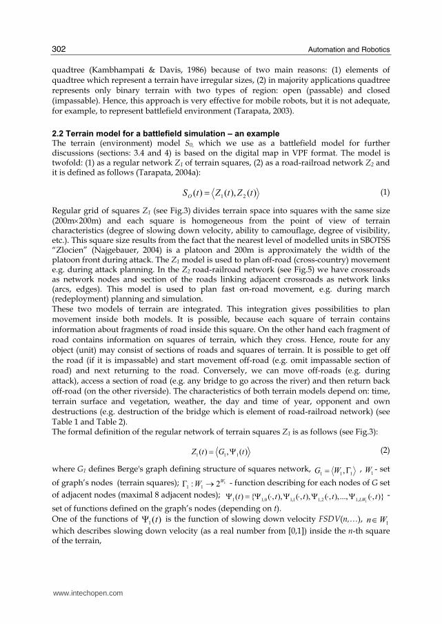
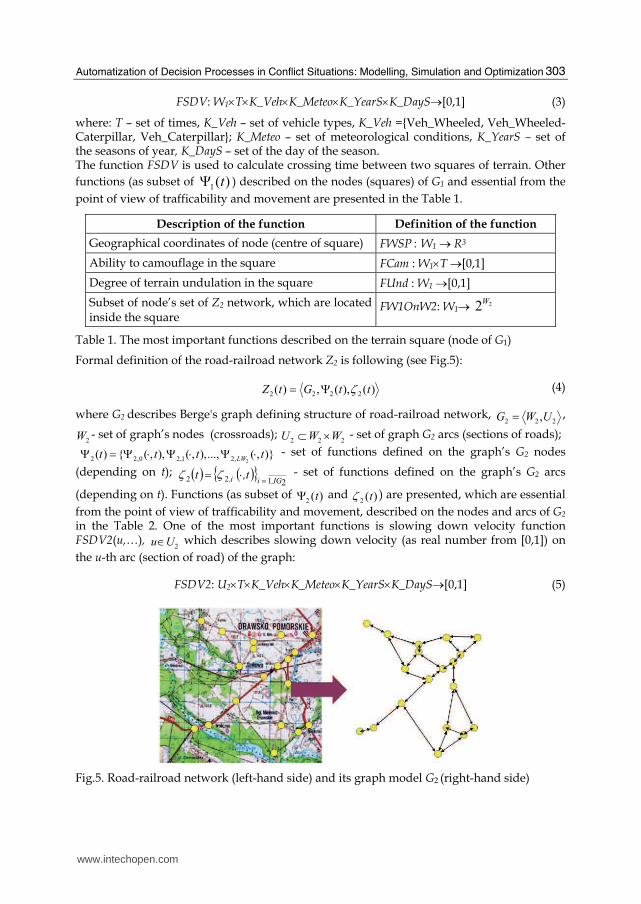
2.2 Terrain model for a battlefield simulation – an example The terrain (environment) model S0, which we use as a battlefield model for further discussions (sections: 3.4 and 4) is based on the digital map in VPF format. The model is twofold: (1) as a regular network Z1 of terrain squares, (2) as a road-railroad network Z2 and it is defined as follows (Tarapata, 2004a):
)(),()( 21 tZtZtSO = (1)
Regular grid of squares Z1 (see Fig.3) divides terrain space into squares with the same size (200m×200m) and each square is homogeneous from the point of view of terrain characteristics (degree of slowing down velocity, ability to camouflage, degree of visibility, etc.). This square size results from the fact that the nearest level of modelled units in SBOTSS “Zlocien” (Najgebauer, 2004) is a platoon and 200m is approximately the width of the platoon front during attack. The Z1 model is used to plan off-road (cross-country) movement e.g. during attack planning. In the Z2 road-railroad network (see Fig.5) we have crossroads as network nodes and section of the roads linking adjacent crossroads as network links (arcs, edges). This model is used to plan fast on-road movement, e.g. during march (redeployment) planning and simulation. These two models of terrain are integrated. This integration gives possibilities to plan movement inside both models. It is possible, because each square of terrain contains information about fragments of road inside this square. On the other hand each fragment of road contains information on squares of terrain, which they cross. Hence, route for any object (unit) may consist of sections of roads and squares of terrain. It is possible to get off the road (if it is impassable) and start movement off-road (e.g. omit impassable section of road) and next returning to the road. Conversely, we can move off-roads (e.g. during attack), access a section of road (e.g. any bridge to go across the river) and then return back off-road (on the other riverside). The characteristics of both terrain models depend on: time, terrain surface and vegetation, weather, the day and time of year, opponent and own destructions (e.g. destruction of the bridge which is element of road-railroad network) (see Table 1 and Table 2). The formal definition of the regular network of terrain squares Z1 is as follows (see Fig.3):
1 1 1( ) , ( )Z t G t= Ψ (2)
where G1 defines Berge's graph defining structure of squares network, 111 ,Γ= WG ,
1W - set
of graph’s nodes (terrain squares); 12: 11
WW →Γ - function describing for each nodes of G set
of adjacent nodes (maximal 8 adjacent nodes); 11 1,0 1,1 1,2 1, ( ) { ( , ), ( , ), ( , ),..., ( , )}LWt t t t tΨ = Ψ ⋅ Ψ ⋅ Ψ ⋅ Ψ ⋅ -
set of functions defined on the graph’s nodes (depending on t).
One of the functions of )( 1 tΨ is the function of slowing down velocity FSDV(n,…), 1Wn∈
which describes slowing down velocity (as a real number from [0,1]) inside the n-th square of the terrain,
www.intechopen.com
Automatization of Decision Processes in Conflict Situations: Modelling, Simulation and Optimization
303
FSDV: W1×T×K_Veh×K_Meteo×K_YearS×K_DayS→[0,1] (3)
where: T – set of times, K_Veh – set of vehicle types, K_Veh ={Veh_Wheeled, Veh_Wheeled-Caterpillar, Veh_Caterpillar}; K_Meteo – set of meteorological conditions, K_YearS – set of the seasons of year, K_DayS – set of the day of the season. The function FSDV is used to calculate crossing time between two squares of terrain. Other
functions (as subset of )( 1 tΨ ) described on the nodes (squares) of G1 and essential from the
point of view of trafficability and movement are presented in the Table 1.
Description of the function Definition of the function
Geographical coordinates of node (centre of square) FWSP : W1 → R3
Ability to camouflage in the square FCam : W1×T →[0,1]
Degree of terrain undulation in the square FUnd : W1 →[0,1]
Subset of node’s set of Z2 network, which are located inside the square
FW1OnW2: W1→ 22W
Table 1. The most important functions described on the terrain square (node of G1)
Formal definition of the road-railroad network Z2 is following (see Fig.5):
)(),(,)( 2222 ttGtZ ζΨ= (4)
where G2 describes Berge's graph defining structure of road-railroad network, 222 ,UWG = ,
2W - set of graph’s nodes (crossroads); 222 WWU ×⊂ - set of graph G2 arcs (sections of roads);
22 2,0 2,1 2, ( ) { ( , ), ( , ),..., ( , )}LWt t t tΨ = Ψ ⋅ Ψ ⋅ Ψ ⋅ - set of functions defined on the graph’s G2 nodes
(depending on t); ( ) ( ){ }2122 IG,ii, t,t =⋅= ζζ - set of functions defined on the graph’s G2 arcs
(depending on t). Functions (as subset of )( 2 tΨ and )( 2 tζ ) are presented, which are essential
from the point of view of trafficability and movement, described on the nodes and arcs of G2 in the Table 2. One of the most important functions is slowing down velocity function FSDV2(u,…),
2Uu∈ which describes slowing down velocity (as real number from [0,1]) on
the u-th arc (section of road) of the graph:
FSDV2: U2×T×K_Veh×K_Meteo×K_YearS×K_DayS→[0,1] (5)
Fig.5. Road-railroad network (left-hand side) and its graph model G2 (right-hand side)
www.intechopen.com

Automation and Robotics
304
Description of the function Definition of the function
Geographical coordinates of node (crossroad) FWSP2 : W2 → R3
Node Z1, which contains node Z2 FW2OnW1: W2 → W1
Subset of set of nodes of the Z1 network, which contains the arc
FU2OnW1: U2 → 12W
Degree of terrain undulation on the arc FUnd : U2→[0,1]
Arc length FLen : U2→R+
Table 2. The most important functions described on the crossroads and on part of the roads (G2)
2.3 Paths planning algorithms in terrain-based simulation
There are four main approaches that are used in a battlefield simulation (CGF systems) for paths planning (Karr et al., 1995): free space analysis, vertex graph analysis, potential fields and grid-based algorithms. In the free space approach, only the space not blocked and occupied by obstacles is represented. For example, representing the centre of movement corridors with Voronoi diagrams (Schiavone et al., 1995) is a free space approach (see Fig.1). The advantage of Voronoi diagrams is that they have efficient representation. Disadvantages of Voronoi diagrams are as follows: they tend to generate unrealistic paths (paths derived from Voronoi diagrams follow the centre of corridors while paths derived from visibility graphs clip the edges of obstacles); the width and trafficability of corridors are typically ignored; distance is generally the only factor considered in choosing the optimal path. In the vertex graph approach, only the endpoints (vertices) of possible path segments are represented (Mitchell, 1999). Advantages of this approach: it is suitable for spaces that have sufficient obstacles to determine the endpoints. Disadvantages are as follows: determining the vertices in “open” terrain is difficult; trafficability over the path segment is not represented; factors other than distance can not be included in evaluating possible routes. In the potential field approach, the goal (destination) is represented as an “attractor”, obstacles are represented by “repellors”, and the vehicles are pulled toward the goal while being repelled from the obstacles. Disadvantages of this approach: the vehicles can be attracted into box canyons from which they can not escape; some elements of the terrain may simultaneously attract and repel. In the regular grid approach, the grid overlays the terrain, terrain features are abstracted into the grid, and the grid rather than the terrain is analyzed. Advantages are as follows: analysis simplification. Disadvantages: “jagged” paths are produced because movement out of a grid cell is restricted to four (or eight) directions corresponding to the four (or eight) neighbouring cells; granularity (size of the grid cells) determines the accuracy of terrain representation. Many route planners in the literature are based on the off-line path planning algorithms: a path for the object is determined before its movement. The following are exemplary algorithms of this approach: Dijkstra’s shortest path algorithm, A* algorithm (Korf, 1999), geometric path planning algorithms (Mitchell, 1999) or its variants (Korf, 1999; Logan, 1997; Logan & Sloman, 1997; Rajput & Karr, 1994; Tarapata, 1999; 2001; 2003; 2004; Undeger et al., 2001). For example, A* has been used in a number of Computer Generated Forces systems as the
www.intechopen.com

Automatization of Decision Processes in Conflict Situations: Modelling, Simulation and Optimization
305
basis of their component planning, to plan road routes (Campbell et al., 1995), to avoid moving obstacles (Karr et al., 1995), to avoid static obstacles (Rajput & Karr, 1994) and to plan concealed routes (Longtin & Megherbi, 1995). Moreover, the multicriteria approach to the path determined in CGF systems is often used. Some results of selected multicriteria paths problem and analysis of the possibility to use them in CGF systems are described, e.g. in (Tarapata, 2007a). Very extensive discussion related to geometric shortest path planning algorithms was presented by Mitchell in (Mitchell, 1999) (references consist of 393 papers and handbooks). The geometric shortest path problem is defined as follows: given a collection of obstacles, find an Euclidean shortest obstacle-avoiding path between two given points. Mitchell considers the following problems: geodesic paths in a simple polygon; paths in a polygonal domain (searching the visibility graph, continuous Dijkstra’s algorithm); shortest paths in other metrics (Lp metric, link distance, weighted region metric, minimum-time paths, curvature-constrained shortest paths, optimal motion of non-point robots, multiple criteria optimal paths, sailor’s problem, maximum concealment path problem, minimum total turn problem, fuel-consuming problem, shortest paths problem in an arrangement); on-line algorithms and navigation without map; shortest paths in higher dimensions. The basic idea of the on-line path planning algorithms (Korf, 1999), in general, is that the object is moved step-by-step from cell to cell using a heuristic method. This approach is borrowed from robots motion planning (Behnke, 2003; Kambhampati & Davis, 1986; LaValle, 2006; Logan & Sloman, 1997; Undeger et al., 2001). The decision about the next move (its direction, speed, etc.) depends on the current location of the object and environment status. Examples of on-line path planning algorithms (Korf, 1999): RTA* (Real-Time A*), LRTA* (Learning RTA*), RTEF (Real-Time Edge Follows), HLRTA*, eFALCONS. For example, the idea of RTEF (real-time edge follow) algorithm (Undeger et al., 2001) is to let the object eliminate closed directions (the directions that cannot reach the target point) in order to decide on which way to go (open directions). For instance, if the object has a chance to realize that moving north and east won’t let him reach the goal state, then it will prefer going south or west. RTEF finds out these open and closed directions by decreasing the number of choices the object has. However, the on-line path planning approach has one basic disadvantage: in this approach using a few criterions simultaneously to find an optimal (or acceptable) path is difficult and it is rather impossible to estimate, the moment of reaching the destination in advance. Moreover, it does not guarantee finding optimal solutions and even suboptimal ones may significantly differ from acceptable.
3. Automatization of main battlefield decision processes
3.1 Introduction
In this section the idea and model of command and control process applied for the decision automata for attack and defence on the battalion level are considered. In section 4 we will complete the description of the automata for the third type of unit task – march. As it was written in section 1 these problems are very rarely discussed in the literature; however some ideas we can come across in (Dockery & Woodcock et al., 1993; Hoffman H. & Hoffman M., 2000). The decision automata being presented replaces battalion commanders in the simulator for military trainings and it executes two main processes (Antkiewicz et al., 2003; Antkiewicz et al., 2007): decision planning process and direct combat control. The decision planning process (DPP) contains three stages: the identification of a decision situation, the
www.intechopen.com

Automation and Robotics
306
generation of decision variants, the variants evaluation and the selection of the best variant, which satisfy the proposed criteria. The decision situation is classified according to the following factors: own task, expected actions of opposite forces, environmental conditions – terrain, weather, the day and season, current state of own and opposite forces in a sense of personnel and weapon systems. For this reason, we can define identification of the decision situation (the first stage of the DPP and the most interesting from the point of view of automatization process) as a multicriteria weighted graph similarity decision problem (MWGSP) (Tarapata, 2007b) and present it in sections 3.3 and 3.4 presenting them through a short overview of structural objects similarity (section 3.2). The remaining two stages of DPP (the variants evaluation and selecting the best variant) are described in detail in (Antkiewicz et al., 2003; Antkiewicz et al., 2007): for each class of decision situations a set of action plan templates for subordinate and support forces are generated. For example the proposed action plan contains (Antkiewicz et al, 2007): forces redeployment, regions of attack or defence, or manoeuvre routes, intensity of fire for different weapon systems, terms of supplying military materiel to combat forces by logistics units. In order to generate and evaluate possible variants the pre-simulation process based on some procedures: forces attrition procedure, slowing down rate of attack procedure, utilization of munitions and petrol procedure is used. In the evaluation process the following criteria: time and degree of task realization, own losses, utilization of munitions and petrol are applied.
3.2 Structural objects similarity – a short overview
Object similarity is an important issue in applications such as e.g. pattern recognition. Given a database of known objects and a pattern, the task is to retrieve one or several objects from the database that are similar to the pattern. If graphs are used for object representation this problem turns into determining the similarity of graphs, which is generally referred to as graph matching. Standard concepts in graph matching include (Farin et al., 2003; Kriegel & Schonauer, 2003): graph isomorphism, subgraph isomorphism, graph homomorphism, maximum common subgraph, error-tolerant graph matching using graph edit distance (Bunke, 1997), graph’s vertices similarity, histograms of the degree sequence of graphs. A large number of applications of graph matching have been described in the literature (Bunke, 2000; Kriegel & Schonauer, 2003; Robinson, 2004). One of the earliest applications was in the field of chemical structure analysis. More recently, graph matching has been applied to case-based reasoning, machine learning planning, semantic networks, conceptual graph, monitoring of computer networks, synonym extraction and web searching (Blondel et al., 2004; Kleinberg, 1999; Kriegel & Schonauer, 2003; Robinson, 2004; Senellart & Blondel, 2003). Numerous applications from the areas of pattern recognition and machine vision have been reported (Bunke, 2000; Champin & Solon, 2003; Melnik et al., 2002). They include recognition of graphical symbols, character recognition, shape analysis, three-dimensional object recognition, image and video indexing and others. It seems that structural similarity is not sufficient for similarity description between various objects. The arc in the graph gives only binary information concerning connection between two nodes. And what about, for example, the connection strength, connection probability or other characteristics? Thus, the weighted graph matching problem is defined, but in the literature it is relatively rarely considered (Almohamad et al., 1993; Champin & Solon, 2003; Tarapata, 2007b; Umeyama, 1988) and it is most often regarded as a special case of graph edit distance, which is a very time-complex measure
www.intechopen.com
Automatization of Decision Processes in Conflict Situations: Modelling, Simulation and Optimization
307
(Bunke, 2004; Kriegel & Schonauer, 2003). Therefore, in section 3.3 we will define a multicriteria weighted graph similarity decision problem (MWGSP) and we will show how to use it for pattern recognition (matching) of decision situations (PRDS) in decision automata, which replaces commanders in simulators for military trainings (Antkiewicz et al., 2007).
3.3 Definition of the multicriteria weighted graph similarity problem (MWGSP)
3.3.1 Structural and quantitative similarity measures between weighted graphs
Let us define weighted graph WG as follows:
{1,..., } {1,..., },{ ( )} ,{ ( )}
G G
i i LF j j LHn N a A
WG G f n h a∈ ∈∈ ∈= (6)
where: G – Berge’s graph, ,G G
G N A= , NG, AG – sets of graph’s nodes and arcs,
{ }, ' : , 'G GA n n n n N⊂ ∈ , : n
i Gf N R→ – the i-th function described on the graph’s nodes,
1,...i LF= , (LF – number of node’s functions); : n
j Gh A R→ – the j-th function described on
the graph’s arcs, 1,...j LH= (LH – number of arc’s functions).
Let two weighted graphs GA and GB be given. We propose to calculate two types of similarities of the GA and GB: structural and non-structural (quantitative). To calculate structural similarity between GA and GB it is proposed to use approach defined in (Blondel et al., 2004). Let A and B be the transition matrices of GA and GB. We calculate following sequence of matrices:
1 , 0
T T
k k
k T T
k k F
BZ A A Z BZ k
BZ A A Z B+
+= ≥+ (7)
where Z0=1 (matrix with all elements equal 1); xT – matrix x transposition; F
x - Frobenius
(Euclidian) norm for matrix x, 2
1 1
B An n
ijFi j
x x= =
= ∑∑ , nB – number of matrix rows (number of
nodes of GB), nA – number of matrix columns (number of nodes of GA). Element zij of the matrix Z describes similarity score between the i-th node of the GB and the j-th node of the GA. The essence of the graph’s nodes similarity is the fact that two graphs’ nodes are similar if their neighbouring nodes are similar. The greater value of zij the greater the similarity between the i-th node of the GB and the j-th node of the GA. We obtain structural similarity matrix S(GA,GB) between nodes of graphs GA and GB as follows (Blondel et al., 2004):
2( , ) [ ] lim
B AA B ij n n kk
S G G s Z× →+∞= = (8)
Some computation aspects of calculation S(GA,GB) have been presented in (Blondel et al., 2004). We can write (7) more explicit by using the matrix-to-vector operator that develops a matrix into a vector by taking its columns one by one. This operator, denoted vec, satisfies
the elementary property vec(C X D)=(DT⊗CT) vec(X) in which ⊗ denotes the Kronecker product (also denoted tensorial, direct or categorial product). Then, we can write equality (7) as follows:
www.intechopen.com

Automation and Robotics
308
1
( )
( )
T T
k
k T T
k F
A B A B zz
A B A B z+
⊗ + ⊗= ⊗ + ⊗ (9)
Unfortunately, the iteration zk+1 does not always converge. Authors of (Melnik et al., 2002)
showed that if we change the formula (9) for 1
( )
( )
T T
k
k T T
k F
A B A B z bz
A B A B z b+
⊗ + ⊗ += ⊗ + ⊗ + , then the
formula (9) converges for b>0. Having matrix S(GA,GB), we can formulate and solve an optimal assignment problem (using e.g. Hungarian algorithm) to find the best allocation
matrix [ ]B Aij n nX x ×= of nodes from graph describing GA, GB:
1 1
( , ) maxB An n
S A B ij ij
i j
d G G s x= =
= ⋅ →∑∑ (10)
with constraints:
1
1, 1,Bn
ij A
i
x j n=
≤ =∑ (11)
1
1, 1,An
ij B
j
x i n=
≤ =∑ (12)
{1,..., } {1,..., }
{0,1}B A
iji n j n
x∈ ∈∀ ∀ ∈ (13)
The dS(GA,GB) describes the value of structural similarity measure of GA and GB (Fig.6).
Fig.6. Examples of weighted graphs with a single function described on the nodes (set of functions described on the arcs is empty) and their structural (S(GA,G)) and quantitative
( *
1( , )
AV G G ) similarity matrices. Filled cells describe ones, which create optimal assignment
the nodes of GA to nodes of G.
www.intechopen.com

Automatization of Decision Processes in Conflict Situations: Modelling, Simulation and Optimization
309
To calculate non-structural (quantitative) similarity between GA and GB we should consider
similarity between values of node’s and arc’s functions (nodes and arcs quantitative similarity).
To compute nodes quantitative similarity we propose to create vector 1( , ) ,...,A B LFG G V V=v
of matrices, where ( )B A
k ij n nV v k ×⎡ ⎤= ⎣ ⎦ , k=1,…,LF, describing similarity matrix between nodes
of GA and GB from the point of view of the k-th node’s function ( :A
A n
k Gf N R→ for GA and
:B
B n
k Gf N R→ for GB) and ( ) ( ) ( )B A
ij k kv k f i f j= − describes “distance” between the i-th node
of GB and the j-th node of GA from the point of view of B
kf and A
kf , respectively. We can
apply a norm with parameter 1p ≥ as distance measure:
1
, ,
1
( ) ( ) ( ) ( ) ( ) ( )
ppn
B A B A B A
k k k k k r k rpr
f i f j f i f j f i f j=
⎛ ⎞− = − = −⎜ ⎟⎜ ⎟⎝ ⎠∑ (14)
where , ( )A
k rf ⋅ , , ( )B
k rf ⋅ describe the r-th component of the vector being value of A
kf and B
kf ,
respectively. Next, we compute for each k=1,…,LF normalized matrix * * ( )B A
k ij n nV v k ×⎡ ⎤= ⎣ ⎦ ,
where * ( ) ( )ij ij k Fv k v k V= . This procedure guarantees that each * ( ) [0,1]ijv k ∈ . Finally, we
compute total quantitative similarity between the i-th node of GB and the j-th node of GA as
follows:
*
1,...,1 1
( ), 1, [0,1]LF LF
ij k ij k kk LF
k k
v v kλ λ λ== == ⋅ = ∀ ∈∑ ∑ (15)
The dQN(GA,GB) nodes quantitative similarity measure of GA and GB we compute solving
assignment problem (10)-(12) substituting ijv− for sij (because of that the smaller value of ijv
the better) and dQN(GA,GB) for dS(GA,GB) in (10). Example of calculations similarity matrices
between nodes of some graphs and similarity measures dS and dQN between graphs are
presented in the Fig.6 and in the Table 3. Let us note that the best structural matched graph
to GA is GB (dS(GA,GB)=1.423 is the maximal value among of values of this measure for other
graphs) but the best quantitative matched graph to GA is GC (dQN(GA,GC)=0 is minimal value
among of values of this measure for other graphs). Question is: which graph is the most
similar to GA : GB or GC? Some method for solving the problem and to answer the question is
presented in section 3.3.2: we have to apply multicriteria choice of the best matched graph to
GA. We can obtain arcs quantitative similarity measure dQA(GA,GB) by analogy to dQN(GA,GB): we
build vector 1( , ) ,...,A B LHG G E E=e of matrices, where [ ( )]
B Ak ij m mE e k ×= , k=1,…,LH (mA, mB –
number of arcs in GA and GB) describing similarity matrix between arcs of GA and GB from
the point of view of the k-th arc’s function ( :A
A n
k Gh A R→ for GA and :B
B n
k Gh A R→ for GB),
( ) ( ) ( )B A
ij k k pe k h i h j= − , next * ( ) ( )ij ij k F
e k e k E= and *
1
( ),LH
ij k ij
k
e e kμ=
= ⋅∑ 1
1,LH
k
k
μ=
=∑ 1,...,
0kk LH
μ= ∀ ≥ .
Substituting in (10) ije− for sij, dQA(GA,GB) for dS(GA,GB) and solving (10)-(12) we obtain
dQA(GA,GB).
www.intechopen.com

Automation and Robotics
310
Graph G dS(GA,G) dQN(GA,G) 0.5dS(GA,G) - 0.5dQN(GA,G)
GB 1.423 0.5 0.462
GC 1.412 0 0.706
GD 1.412 0.25 0.456
GE 1.225 0.5 0.362
Table 3. Values of similarity measures between GA and each of the four graphs from Fig.6
Let us note that it is possible to determine single quantitative similarity measure for GA and
GB . To this end we use some transformation of graph ,G N A= into temporary graph
* * *,G N A= as follows: *N N A= ∪ , * * *
A N N⊂ × and
( )( )
*
,
*
( , ) ( , )
( , ) ( , )
v N a A x N
x N
v x a v a A
x v a a v A
∈ ∈ ∈
∈
∀ ∃ = ⇒ ∈ ∨∃ = ⇒ ∈
(16)
If G was a weighted graph then in G* we attribute the arc’s and node’s functions from G to
appropriate nodes of G* (that is to nodes and arcs from G). Using this procedure for GA and
GB we obtain *
AG and *
BG . Next, for *
AG and *
BG we can calculate nodes quantitative
similarity measure * *( , )QN A Bd G G . Example of constructing G* from G is presented in the Fig.7.
Fig.7. Transformation of G (left-hand side) into G* (right-hand side)
3.3.2 Formulation of multicriteria weighted graphs similarity problem (MWGSP)
Let us accept 1 2
{ , ,..., }M
SG G G G= as a set of weighted graphs defining certain objects.
Moreover, we have weighted graph P that defines a certain pattern object. The problem is to
find such a graph Go from SG that is the most similar to P. We define this problem as a
multicriteria weighted graphs similarity problem (MWGSP), which is a multicriteria
optimization problem in the space SG with relation RD:
( ), , DMWGSP SG F R= (17)
where 3:F SG R→ , ( ) ( )( , ), ( , ), ( , )S QN QA
F G d P G d P G d P G= and
www.intechopen.com

Automatization of Decision Processes in Conflict Situations: Modelling, Simulation and Optimization
311
( , ) : ( , ) ( , )
( , ) ( , )
( , ) ( , )
S S
D QN QN
QA QA
Y Z SG SG d P Y d P Z
R d P Y d P Z
d P Y d P Z
⎧ ⎫∈ × ≥ ∧⎪ ⎪= ≤ ∧⎨ ⎬⎪ ⎪≤⎩ ⎭ (18)
Domination relation RD (Pareto relation between elements of SG) gives possibilities to compare graphs from SG. Weighted graph Z is more similar to P than Y if structural similarity between P and Y is not smaller than between P and Z and, simultaneously, both quantitative similarities between P and Y are not greater than between P and Z. There are many methods for solving the problem (17) (Eschenauer et al., 1990): weighted sum (scalarization of set of objectives), hierarchical optimization (the idea is to formulate a sequence of scalar optimization problems with respect to the individual objective functions subject to bounds on previously computed optimal values), trade-off method (one objective is selected by the user and the other ones are considered as constraints with respect to individual minima), method of distance functions in Lp-norm ( 1p ≥ ) and others. We
propose to use scalar function ( ) :H G SG R→ as weighted sum of objectives:
( ) ( ) ( )1 2 3
1 2 3 1 2 3
( , ) ( , ) ( , )
, , 0, 1
S QN QAH G d P G d P G d P Gα α αα α α α α α
= ⋅ + ⋅ − + ⋅ −≥ + + = (19)
Taking into account (19) the problem of finding the most matched Go to pattern P can be
formulated as follows: to determine such a oG SG∈ , that ( ) max ( )o
G SG
H G H G∈
= . In the last
column of the Table 3 the scalar function H(G) is defined as follows:
1 2 3( ) ( , ) ( ( , )) ( ( , ))S QN QAH G d P G d P G d P Gα α α= ⋅ + ⋅ − + ⋅ − (20)
where 1 2 0.5α α= = ,
3 0, AP Gα = = , { , , , }B C D ESG G G G G= . Let us note that the best matched
graph to GA being solution of MWGSP with scalar function H(G) is GC (H(Go=GC)=0.706). In the paper (Tarapata, 2007b) epsilon-similarity of weighted graphs as another view on quantitative similarity between weighted graphs is additionally considered.
3.4 Application of weighted graphs similarity to pattern recognition of decision situations
For the identification of the decision situation described in section 3.1 we define decision situations space as follows:
1,..,1,..,
: [ ]ij i Xj Y
DSS SD SD SD ==⎧ ⎫= =⎨ ⎬⎩ ⎭ (21)
where SD denotes net of terrain squares as a model of activities (interest) area
1,..,8( )k
ij ij kSD SD == . For the terrain square with the indices (i,j) each of elements denotes:
1
ijSD - the degree of terrain passability, 2
ijSD - the degree of forest covering, 3
ijSD - the
degree of water covering, 4
ijSD - the degree of terrain undulating, 5
ijSD - armoured power
(potential) of opposite units deployed in the square, 6
ijSD - infantry power (potential) of
www.intechopen.com

Automation and Robotics
312
opposite units deployed in the square, 7
ijSD - artillery power (potential) of opposite units
deployed in the square, 8
ijSD - coordinates of square, X - the width of an activities (interest)
area (number of squares), Y - the depth of an activities (interest) area (number of squares)
and [0,1], 1,...,7k
ijSD k∈ = , 8 2
ijSD R+∈ . Moreover, we have set PDSS of decision situations
patterns written in the database, { : }PDSS PS PS DSS= ∈ and current situation CS DSS∈ .
The problem is: to find the most similar PS PDSS∈ to current situation CS DSS∈ .
In the presented proposition the weighted graphs similarity approach to identification of decision situation is used. It consists of three stages: 1. Building weighted graphs WGT(CS), WGD(CS) and WGT(PS), WGD(PS) representing
decision situations: current (CS) and pattern (PS) for topographical conditions (WGT) and units (potential) deploying (WGD);
2. Calculation of similarity measures between pairs: WGT(CS), WGT(PS) and WGD(CS),
WGD(PS) for each PS PDSS∈ ;
3. Selecting the most similar PS to CS using calculated similarity measures. Stage 1 The first stage is to build weighted graphs WGT and WGD as follows:
{1,...,5}, ,{ ( )}GT
T
GT GT k kn N
WGT GT N A f n ∈∈= = ,
{1,...,4}, ,{ ( )}GD
D
GD GD k kn N
WGD GD N A f n ∈∈= =
where G (GT or GD) – Berge’s graphs, ,G GG N A= , NG, AG – sets of graph’s nodes and arcs,
{ }, ' : , 'G GA n n n n N⊂ ∈ . Weighted graphs WGT and WGD describe decision situations
(current CS and pattern PS). Each node n of GT and GD describes terrain cells (i,j)=n with
non-zero values of characteristics defined as components of ij
SD from (21) and
{1,...,4}( ) ,T k
k ijk
f n SD∈∀ = 8
5 ( )T
ijf n SD= , 4
{1,...,3}( )D k
k ijk
f n SD +∈∀ = , 8
4 ( )D
ijf n SD= . Two nodes , GDx y N∈
(for , GTx y N∈ by analogy) are linked by an arc, when cells represented by x and y are
adjacent (more precisely: they are adjacent cells that taking into account the direction of
action, see Fig.8). For example, the terrain can be divided into 15 cells (3 rows and 5
columns, left-hand side, see Fig.8). The units are located in some cells (denoted by circles
and Xs). Structural representation of deployment of units is defined by the graph GD. Let us
note that similar representation can be used for topographical conditions (single graph for
one of the topographical information layer: waters, forests, passability or single graph GT
for all of this information, see Fig.8, right-hand side).
Stage 2 Having weighted graphs WGD(CS) and WGD(PS) (WGT(CS) and WGT(PS)) representing
current CS and pattern PS decision situations (for units deploying) we use the procedure
described in section 3.3.1 to calculate structural and quantitative similarity measures for
both graphs. We obtain for WGD: dS(WGD(CS), WGD(PS))= ( , )D
Sd CS PS , dQN(WGD(CS),
WGD(PS))= ( , )D
QNd CS PS and for WGT: dS(WGT(CS),WGT(PS))= ( , )T
Sd CS PS ,
dQN(WGT(CS),WGT(PS))= ( , )T
QNd CS PS .
www.intechopen.com

Automatization of Decision Processes in Conflict Situations: Modelling, Simulation and Optimization
313
Fig.8. Deployment of units and their structural (graph GD) representation (left-hand side) and terrain covering (growth) and its structural (GT) representation (right-hand side). Circle (O) and sharp (X) describe two types of units
Stage 3 We formulate problem (17), separately for WGT and WGD, where: SG:=PDSS, F(G):=FD(PS),
( , )Sd P G := ( , )D
Sd CS PS , ( , )QNd P G := ( , )D
QNd CS PS for WGD and F(G):=FT(PS),
( , )Sd P G := ( , )T
Sd CS PS , ( , )QNd P G := ( , )T
QNd CS PS for WGT. Next, we define scalar
functions (19) to solve the problem (17) for WGD and WGT:
1 2( ) ( , ) ( ( , ))D D
D S QNH d dα α⋅ = ⋅ ⋅ ⋅ + ⋅ − ⋅ ⋅
and
1 2( ) ( , ) ( ( , ))T T
T S QNH d dγ γ⋅ = ⋅ ⋅ ⋅ + ⋅ − ⋅ ⋅ .
Having HD(PS) and HT(PS) we can combine these criteria (like in (19)) or set some threshold
values and select the most matched pattern situation to the current one.
An example of using the presented approach to find the most matched pattern decision
situation to current one is presented in the Fig.9 and in the Table 4. Results of calculations
HD(PS) are presented for each 1 8{ ,..., }PS PDSS PS PS∈ = . Only function ( ) 8
4 ( )D CS
ijf n SD=
( ( )
4( )D PSf n for pattern PS) is used from WGD to compute nodes quantitative similarity (see
section 3.3.1) because all units have the same type. Thus, vector v(WGD(CS),WGD(PS)) of
matrices has one component ( ) ( )1 | | | |[ (1)]
GD PS GD CSij N NV v ×= . Function ( )
4 ( )D CSf n describes
coordinates of node n (left-lower cell has coordinates (1,1)). The norm from (14) has the form
of: 4 4 2
( ) ( )D D
pf i f j =− =
1 222
4, 4,
1
( ) ( )D D
r r
r
f i f j=
⎛ ⎞−⎜ ⎟⎜ ⎟⎝ ⎠∑ and it describes the geometric distance
between nodes i∈NGD(PS) and j∈NGD(CS). Let us note that for weights 1 20, 1α α= = value in
Table 4 (for the row PSi) describes ( , )D
QN id CS PS and for 1 21, 0α α= = describes
( , )D
S id CS PS . The best matched PS to CS is PS2 (taking into account D
Sd and D
QNd ).
The process of optimal selection of weights can be organized as follows: we build a learning
set {CSi,PDSSi}i=1,…,LS and for different values of weights experts estimate whether, in their
subjective opinion, CSi is similar to PS*∈PDSSi determined from the procedure.
Combination of weight values, which are indicated by majority of experts is the optimal
combination.
www.intechopen.com

Automation and Robotics
314
Fig.9. Current situation CS with graph GD(CS) and eight pattern situations PSi (i=1,…,8) with graphs GD(PSi) describing structure of units deployment. Patterns 1-5, 2-6, 3-7 and 4-8 have the same structure but cells for patterns 5,..,8 have a greater size than for patterns 1,…,4
Pattern Weights (α1 ; α2)
PSi (0; 1) (0.33; 0.67) (0.5; 0.5) (0.67; 0.33) (1; 0)
PS1 -0.094 0.283 0.463 0.800 1.527
PS2 -0.370 0.283 0.593 0.870 1.504
PS3 -0.478 0.157 0.360 0.726 1.254
PS4 -0.233 0.176 0.467 0.827 1.527
PS5 -0.474 0.120 0.461 0.824 1.527
PS6 -0.706 0.032 0.378 0.761 1.504
PS7 -0.63 0.070 0.279 0.631 1.254
PS8 -0.508 0.047 0.415 0.793 1.527
Table 4. Values of scalar function HD(PSi) combining structural (weight α1) and quantitative
(weight α2) similarity measures between GD(CS) and GD(PSi) from Fig.9. The best (maximal) value in the columns are denoted in bold
4. Automatization of march process
4.1 Introduction
The automata for march executes two main processes (Tarapata, 2007c): march planning process and direct march control. The march planning process relating to the automata includes the determination of: march organization (unit order in march column, count and place of stops and rests), paths for units and detailed march schedule for each unit in the column. The direct march control process contains such phases like command, reporting and reaction to fault situations during the march simulation. The automata is implemented in the ADA language and it represents a commander of battalion level (the lowest level of
www.intechopen.com

Automatization of Decision Processes in Conflict Situations: Modelling, Simulation and Optimization
315
trainees is brigade level). It is a component of distributed interactive simulation system SBOTSS “Zlocien” for CAX (Computer Assisted Exercises) (Najgebauer, 2004).
4.2 The march planning process
4.2.1 Description of the problem
The march planning process relating to the automata contains the determination of such elements as: march organization (units order in march column, count and place of stops), paths for units and detailed march schedule for each unit in the column. Algorithms, which carry out the decision planning process described below, are presented in the section 4.4. The decision process for march starts in the moment t, when the battalion id receives the march order SO(id, t) from a superior (brigade) unit. Structure of the SO(id, t) is as follows:
( )0( , ) ( , ), ( , ), ( , )S
SO id t t id t t id t MD id t= (22)
where: SO(id, t) – superior order to march for battalion id; 0 ( , )t id t - readiness time for the
unit id; ( , )St id t - starting time of the march for the unit id; ( , )MD id t - detailed description of
march order. Definition of the ( )MD id (we omit t) is as follows:
( )1,
( ) ( ), ( ), ( ), ( ) ( ), ( )p p p NIPMD id S id D id RP id IP id in id it id == = (23)
where: ( ), ( )S id D id - source and destination areas for id, respectively; RP(id) – rest area for
the id unit (after twenty-four-hours of march), optional; IP(id) – vector of checkpoints for the id unit (march route must cross these points), inp(id) – the p-th checkpoint,
1 2( )
pin id W W∈ ∪ ,
in1(id)=PS(id) is the starting point of the march (at this point the head of the march column is formed) and it is required, other checkpoints are optional, itp(id) – time of achieving the p-th checkpoint (optional); NIP – number of checkpoints. After the id unit (battalion) receives the brigade commander’s order to march, the decision automata starts planning the realization of this task. Taking into account ( , )SO id t , for each unit id’ (of company level and
equivalent) directly subordinate to id the march order, MDS(id’) is determined as follows:
( )( ') ( '), ( '), ( '), ( '), ( '), ', ( '), ( ')MDS id S id D id PS id PD id RP id id S id D idμ= (24)
where: ( '), ( ')S id D id - source and destination areas for id’, respectively, ( ') ( )S id S id⊂ ,
( ') ( )D id D id⊂ ; RP(id’) – rest area for the id’ unit (after twenty-four-hours of march),
( ') ( )RP id RP id⊂ , optional parameter; PS(id’) – starting point for the id’ unit, the same for all
id’∈id and 1 1 2( ') ( )PS id in id W W= ∈ ∪ ; PD(id’) – ending point of the march for the id’ unit, the
same for all id’∈id and 1 2( ')PD id W W∈ ∪ ; ( ', , )id S Dμ - the route for the unit id’ from the
region S(id’)=S to region D(id’)=D, ( )1, ( ( ', , ))
( ', , ) ( ', ), ( ', )m LW id S D
id S D w id m v id m μμ == , ( ', )w id m -
the m-th node on the path for id’, 1 2( ', )w id m W W∈ ∪ , S,D⊂W1∪W2 and
( ',1)w id S∈ , ( )( )', ( ', , )w id LW id S D Dμ ∈ ; LW(μ(id’, S, D)) – number of nodes (squares or
crossroads) on the path μ(id’,S,D) for id’ unit; ( ', )v id m - velocity of the id’ unit on the arc
www.intechopen.com

Automation and Robotics
316
starting in the m-th node. It is important to note that path ( ', , )id S Dμ may consist of
sequences of nodes from Z1(t) and Z2(t) (when we accept descending from the road on the squares (if it is possible) and vice versa).
4.2.2 March organization determination
March organization includes the determination of such elements as: number of columns,
order of units in march columns and number and place of stops.
Number (#) of columns results from tactical rules and depends on the tactical level of the
unit: for the battalion level #columns=1, for the brigade level #columns=1÷3; for the division
level #columns=3÷5. Order of units in march column results from tactical rules as well
(algorithm Units_Order_In_March_Column_Determ(id’), see Table 6). Number of stops
( )stopsc id is calculated as follows (algorithm Number_of_Stops_Determ(id’), see Table 6):
( )( )( , ) ( , ) ( ) ( ) ( )
( ) max ,0( ) ( )
D S rest avg path
stops
avg stop
t id t t id t t id v id L idc id
v id t id s
⎧ ⎫⎢ ⎥− − ⋅ −⎪ ⎪= ⎢ ⎥⎨ ⎬⋅ + Δ⎢ ⎥⎪ ⎪⎣ ⎦⎩ ⎭ (25)
where: ( , )Dt id t - demanded ending time of the march for the id unit, ( , )St id t - starting time
of the march for the id unit (like in (22)), ( , ) ( , ) 0D St id t t id t> ≥ , ( )restt id - duration time of the
rest for the id unit, ( )avgv id - average march velocity for the id unit, ( )pathL id - length of the
path determined for the id unit (in km), ( )stopt id - duration time of the stop for the id unit,
sΔ - time interval between stops. In practice, values of parameters are as follows:
( )restt id ≈24h, [ ]( ) 30 40 km/havgv id ∈ ÷ , ( ) 1 hstopt id ≈ , [ ]3,4 hsΔ ∈ .
Place of stops are fixed after path determination and algorithm Place_Of_Stops_Determ(id’)
(see Table 6) takes into account ( )stopsc id and the FCam function (see Table 1) to find optimal
positions of stops.
4.2.3 Detailed march schedule determination
Detailed movement schedule for id’ unit is defined as follows:
0( ', ) , , ( ', , ), ( ', , )H id t S D id S D T id S Dμ= (26)
where: t0 – starting moment of schedule realization; ( ', , )T id S D - vector of moments of
achieving nodes on the path, 1, ( ( ', , ))
( ', , ) ( ', )m LW id S D
T id S D t id m μ== , ( ', )t id m - moment of
achieving the m-th node on the path,
( )1
0
1
( ', ), ( ', 1)( ', )
( ', )
m
j
L w id j w id jt id m t
v id j
−
=+= +∑ (27)
and L(w(id’,j),w(id’,j+1)) describes geometric distance between the j-th and the (j+1)-st nodes
on the path, LW(μ(id',S,D) - number of nodes on the path for id’ unit. After determining
MDS(id’) for each unit id’ subordinates to battalion id, the order is sent by automata to each
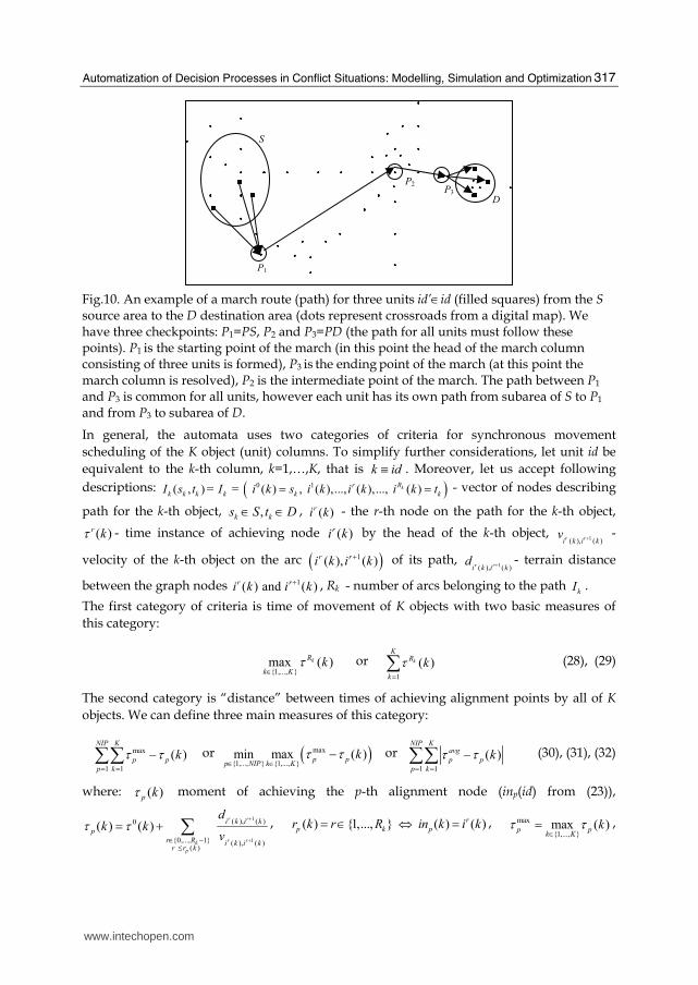
of the id’ units. The idea of determining march route for the unit id is presented in the Fig.10.
www.intechopen.com
Automatization of Decision Processes in Conflict Situations: Modelling, Simulation and Optimization
317
Fig.10. An example of a march route (path) for three units id’∈id (filled squares) from the S source area to the D destination area (dots represent crossroads from a digital map). We have three checkpoints: P1=PS, P2 and P3=PD (the path for all units must follow these points). P1 is the starting point of the march (in this point the head of the march column consisting of three units is formed), P3 is the ending point of the march (at this point the march column is resolved), P2 is the intermediate point of the march. The path between P1 and P3 is common for all units, however each unit has its own path from subarea of S to P1 and from P3 to subarea of D.
In general, the automata uses two categories of criteria for synchronous movement
scheduling of the K object (unit) columns. To simplify further considerations, let unit id be
equivalent to the k-th column, k=1,…,K, that is k id≡ . Moreover, let us accept following
descriptions: ( )0 1( , ) = ( ) , ( ),..., ( ),..., ( )kRr
k k k k k kI s t = I i k s i k i k i k t= = - vector of nodes describing
path for the k-th object, ,k ks S t D∈ ∈ , ( )r
i k - the r-th node on the path for the k-th object,
( )r kτ - time instance of achieving node ( )ri k by the head of the k-th object, 1( ), ( )r ri k i k
v + -
velocity of the k-th object on the arc ( )1( ), ( )r ri k i k+ of its path, 1( ), ( )r ri k i k
d + - terrain distance
between the graph nodes 1( ) and ( )r ri k i k+ , Rk - number of arcs belonging to the path kI .
The first category of criteria is time of movement of K objects with two basic measures of
this category:
{1,..., }max ( )kR
k Kkτ∈ or
1
( )k
KR
k
kτ=∑ (28), (29)
The second category is “distance” between times of achieving alignment points by all of K
objects. We can define three main measures of this category:
max
1 1
( )NIP K
p p
p k
kτ τ= =
−∑∑ or ( )max
{1,..., } {1,..., }min max ( )p p
p NIP k Kkτ τ∈ ∈ − or
1 1
( )NIP K
avg
p p
p k
kτ τ= =
−∑∑ (30), (31), (32)
where: ( )p kτ moment of achieving the p-th alignment node (inp(id) from (23)),
1
1
( ), ( )0
{0,..., 1} ( ), ( ) ( )
( ) ( ) r r
r rk
p
i k i k
p
r R i k i kr r k
dk k
vτ τ +
+∈ −≤= + ∑ , ( ) {1,..., } ( ) ( )r
p k pr k r R in k i k= ∈ ⇔ = , max
{1,..., }max ( )p p
k Kkτ τ∈= ,
S
P1
D
P2 P3
www.intechopen.com
Automation and Robotics
318
1
1( )
Kavg
p p
k
kK
τ τ=
= ∑ . Taking into account that unit id is equivalent to the k-th column we can
write as follows: 1( ), ( )
( , )r ri k i kv v k r+ ≡ , ( ) ( , )ri k w k r≡ , ( )1( ), ( )
( , ), ( , 1)r ri k i kd L w k r w k r+ ≡ + .
One of the formulations of the optimization problem for movement synchronization of K objects using measures (28)-(32) can be defined as follows: for fixed paths Ik of each k-th
object to determine such 1( ), ( )
, 0, 1, 1,r r ki k i kv r R k K+ = − = that
max
1 1
( ) minNIP K
p p
p k
kτ τ= =
− →∑∑ (33)
with the constraints :
1
max
( ), ( )( ), 0, 1, 1,r r ki k i k
v v k r R k K+ ≤ = − = (34)
1( ), ( )
0, 0, 1, 1,r r ki k i kv r R k K+ > = − = (35)
where max ( )v k describes maximal velocity of the k-th object resulting from its technical
properties.
4.2.4 Path determination for march
To find paths for units, modified shortest path algorithms (SPA) such as Dijkstra’s, A*, geometric SPA are used in SBOTSS “Zlocien” (Najgebauer, 2004). Geometric SPA supplements two algorithms presented above (the hybrid shortest path algorithm is obtained) and it is used in case the size of the network is large (default is 10000 nodes, but it is a parameter set in a so-called calibrator of the simulation system (Antkiewicz et al., 2006)). Modifications of mentioned algorithms deal with the following details: (a) paths determination in different configurations - (a1) from point (region) to point (region), (a2) visiting selected points (regions), (a3) omitting selected points (regions, obstacles), (a4) inside or outside selected region, (a5) off-roads only, (a6) on-roads only, (a7) combined on- and off-roads and others; (b) if we do not set the region inside where we want to find the path then the algorithm itself, iteratively determines the rectangular region, which is based on a line linking the beginning and end points (nodes) of movement, to minimize computational time; (c) if we want to find an on-road path only, and there are no nodes of the road network inside the intermediate squares, then the algorithm may optionally find crossroads (nodes of the road network), which are nearest to squares inside that the path must cross. Detailed description of the movement planning algorithms used in SBOTSS “Zlocien” is presented in (Tarapata, 2004a). In general, modelling and optimization of multi-convoy redeployment (for simultaneous movement of many columns) are very complicated processes. Complexity of these processes depends on the following conditions: number of convoys (the greater the number of convoys the more complicated is the scheduling of redeployment); number of objects in each convoy (the longer the convoy the more complicated is the scheduling of redeployment); Have convoys been redeployed simultaneously? Can convoys be destroyed during redeployment? Can the terrain-based network be destroyed during redeployment? Have convoys been redeployed through disjoint routes? Have convoys achieved selected
www.intechopen.com

Automatization of Decision Processes in Conflict Situations: Modelling, Simulation and Optimization
319
positions (nodes) at a fixed time? Do convoys have to start at the same time? Have convoys determined any action strips for moving? Can convoys be joined and separated during redeployment? Do convoys have to cross through fixed nodes?, etc. Some of these aspects are considered in section 4.2.3 and in the papers: (Benton et al., 1995; Cassandras et al. 1995; Karr et al., 1995; Kreitzberg et al., 1990; Logan & Sloman, 1997; Logan, 1997; Longtin & Megherbi, 1995; Mohn, 1994; Pai & Reissell, 1994; Schrijver & Seymour, 1992; Rajput & Karr, 1994; Tarapata, 1999; 2000; 2001; 2003; 2004a; 2005).
4.3 The direct march control
4.3.1 Identifying fault situations during a march simulation and automata reactions
The direct march control process contains such phases as: command, reporting and reaction
to fault situations during march simulation (Tarapata, 2007c). Let us remember that
automata replaces battalion commander and manages subordinate units (company or/and
platoons and equivalent).
The automata for march react to some fault situations during the march simulation presented in the Table 5.
Fault situation during march simulation
Automata reaction
Current velocity of a subordinate unit differs from scheduled velocity
- If the unit is at the head of the column and it does not move at planned velocity then increase the velocity (in case of delay) or decrease it (in case of acceleration); - If the unit is not at the head of column then adapt velocity to velocity of the preceding unit in the column
Achieving critical fuel level in one of the subordinate units
Reporting to automatic commander. Attempt to refuel at the next stop or refuel as soon as possible
Detection of an opponent unit
If opponent forces are overwhelming (opponent combat potential is greater then a threshold value) and distance between own and the opponent units is relatively small then unit is to be stopped, make defence and report to commander. Otherwise, report to commander only
Detection of a minefield stop and report to commander
Loss of capability to carry out the march (destruction of part of the
march route (e.g. bridge, river crossing) or other cause of
impassability)
- If part of the route is impassable due to destruction of part of the march route then attempt to find a detour. Report to commander; - If there is another cause of impassability then make defence and report to commander
Contamination of part of the march route or subordinate unit
Report to commander. If degree of contamination is low then run chemical defence and continue march, otherwise try to exit from the contaminated area
Table 5. Fault situations during march simulation and automata reactions
www.intechopen.com

Automation and Robotics
320
Situations, which require reporting to the superior of the battalion, are as follows: achieving checkpoints, stop area or rest area; slowing down velocity, which causes delays; encountering contamination; encountering a minefield; achieving a fuel level of 75% and 50% of the normative level; loss capability of carrying out the march (reporting cause of capability loss); detection of opponent units. A detailed description of movement synchronization is presented in section 4.3.2.
4.3.2 Velocity calculation We “see” the unit on the road twofold: (1) as occupying arcs (part of the roads) and nodes (crossroads) of the Z2 network, (2) as sequence of squares of the Z1 network by which the arc cross. In the (1) case we move the head and the tail of the column and we register arcs of the Z2 in which the head and the tail are located with degrees of crossing these arcs. In the (2) case we locate the head and the tail of the column on small squares and we move the “snake” of small squares (from the head to the tail). Movement of the unit on the road (deployed in the column) is done by determining the sequence of nodes (crossroads) and arcs (part of the roads) of the Z2 network using algorithms presented in section 4.2 and then we realize movement from crossroad to crossroad. The important problem during simulation is to set the current velocity of the unit id. Procedure of setting the velocity inside the j-th square taking into account two cases: (a) when the unit id does not fight in the j-th square; (b) when the unit id fights in the j-th square. In the (a) case the current velocity vcur(id, j) of the unit id in the j-th square is calculated as follows:
vcur(id,j)=min{ ( ),slowdv id j ,vdec(id,j)} (36)
where: ( ),slowdv id j - maximal velocity of the unit id in the j-th square taking into account
topographical conditions,
( ) max, ( ) ( , )slowdv id j v id FOP id= ⋅ • (37)
)(max idv - maximal possible velocity of the unit id resulting from technical parameters of the
vehicles belonging to this unit, max
( )( ) min ( )tech
p ZVeh idv id v p∈= , ZVeh(id) – set of vehicles belonging
to the id unit, vtech(p) – maximal velocity of vehicle p (resulting from technical parameters), FOP(id,•) - slowing down velocity function for the id unit in the j-th square, FOP(id,•) is equal (3) or (5); vdec(id, j) – velocity resulting from commander decision (equals v(id,j) in (27)). If the unit id is a head of a column and it does not move with planned velocity vdec(id, j) then the velocity is increased (in case of delay) or decreased (in case of acceleration). If the unit id is not at the head of column then velocity of the unit id is adapted to velocity of the preceding unit in the column. In the (b) case the current velocity vcur(id, j) of the unit id in the j-th square is calculated as follows:
( ){ }( , ) min ( , ), , , , ( , )slowd
cur A B decv id j f v id U U dist v id j= • (38)
where: f(•,•,•,•) – function describing velocity in the square depending on vslowd(id,•), potentials of the unit id of side A (UA) and B (UB) which fight, distance (dist) between fighting sides.
www.intechopen.com
Automatization of Decision Processes in Conflict Situations: Modelling, Simulation and Optimization
321
Some results of velocity calculations in real scenario for brigade march are presented in the Table 7.
4.3.3 Fuel consumption calculation
Fuel consumption FC(id, veh, u) on the u part of a path for the type of vehicle veh belonging to the id unit is calculated as follows:
( )( , , ) ( ) ( , ) ( , )
100
NFC vehFC id veh u FLen u FCC u veh N id veh= ⋅ ⋅ ⋅ (39)
where: FLen(u) describes the length of the u part of a path, FCC(u,veh) – fuel consumption coefficient for the u part of a path and for vehicle type veh, NFC(veh) – normative average fuel consumption for the veh type of vehicle (per 100km), N(id, veh) – number of vehicles of veh type in the id unit. Fuel consumption coefficient FCC is calculated as follows:
FCC(u,veh)=(1.0+MTC(veh))*(1.0+ UC(u)) (40)
where MTC(veh) describes mechanical-tactical coefficient and UC(u) - utilization coefficient,
veh∈K_Veh resulting from logistic calculations.
4.4 Automata implementation
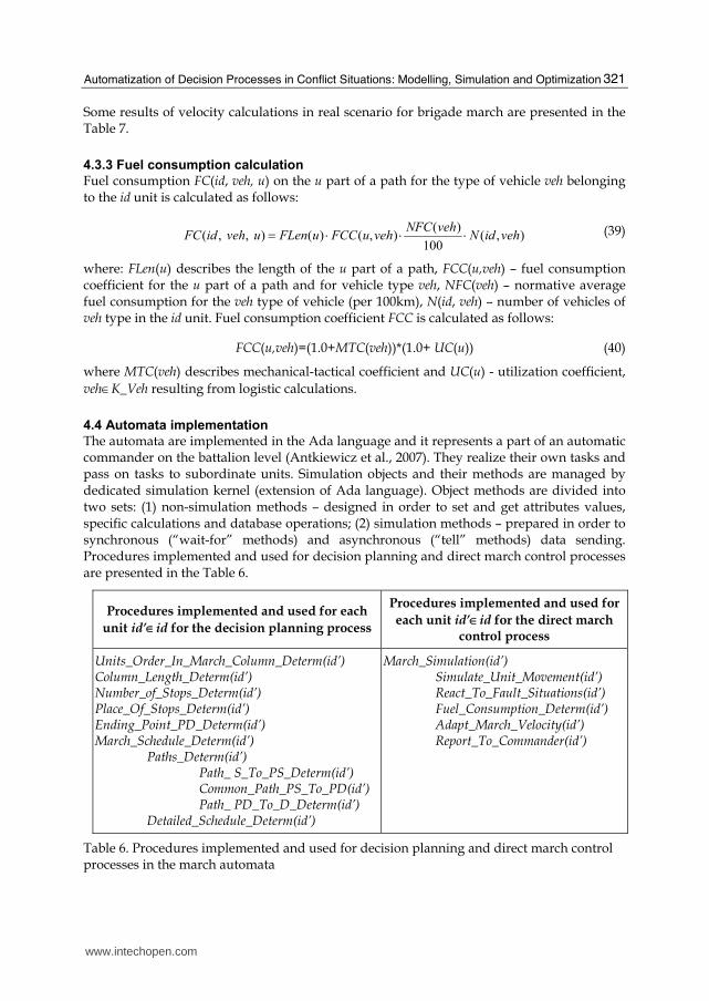
The automata are implemented in the Ada language and it represents a part of an automatic commander on the battalion level (Antkiewicz et al., 2007). They realize their own tasks and pass on tasks to subordinate units. Simulation objects and their methods are managed by dedicated simulation kernel (extension of Ada language). Object methods are divided into two sets: (1) non-simulation methods – designed in order to set and get attributes values, specific calculations and database operations; (2) simulation methods – prepared in order to synchronous (“wait-for” methods) and asynchronous (“tell” methods) data sending. Procedures implemented and used for decision planning and direct march control processes are presented in the Table 6.
Procedures implemented and used for each
unit id’∈id for the decision planning process
Procedures implemented and used for
each unit id’∈id for the direct march control process
Units_Order_In_March_Column_Determ(id’) Column_Length_Determ(id’) Number_of_Stops_Determ(id’) Place_Of_Stops_Determ(id’) Ending_Point_PD_Determ(id’) March_Schedule_Determ(id’) Paths_Determ(id’) Path_ S_To_PS_Determ(id’) Common_Path_PS_To_PD(id’) Path_ PD_To_D_Determ(id’) Detailed_Schedule_Determ(id’)
March_Simulation(id’) Simulate_Unit_Movement(id’) React_To_Fault_Situations(id’) Fuel_Consumption_Determ(id’) Adapt_March_Velocity(id’) Report_To_Commander(id’)
Table 6. Procedures implemented and used for decision planning and direct march control processes in the march automata
www.intechopen.com

Automation and Robotics
322
4.5 Practical example
In this section a practical example of march planning and simulation is presented. In Fig.11a
initial tactical situation is shown. In our example 2 mechanized brigades (121BZ and 123BZ:
each of the brigades consists of 4 mechanized battalion x 4 mechanized companies) of the
blue side receive order to march.
(a) (b) (c)
Fig.11. (a) Initial tactical situation, 4:00am: two mechanized brigades of the “blue” side (121BZ and 123BZ) receive an order to march; (b) Location of the 121 BZ on the road, 5:50am; (c) Location of the 123 BZ on the road, 5:50am
In the superior order (22): destination area for 121BZ and 123BZ is set to about 30 km to the
north of the northern edge of the location area of the red side; distance from source area S to
destination area D is equal about 110km; 5 checkpoints is set.
In the Fig.11b and Fig.11c location of 121BZ and 123BZ, respectively, after nearly 2 hours of
march are presented.
Initial redeploying of the blue side is presented in Fig.12a. 121BZ is redeployed on the
northern-east of the blue force redeploying area. 123 BZ is redeployed on the south of 121
BZ. The location of 121BZ and 123BZ at 5.50am is shown in Fig.12b.
Fig.12. (a) Initial redeployment of the blue side, 4:00am; (b) Location of 121 BZ and 123 BZ, 5:50am
Presented in Table 7 are the average velocities between selected march checkpoints for
121BZ and 123BZ. Average march velocity is equal to about 30km/h.
www.intechopen.com

Automatization of Decision Processes in Conflict Situations: Modelling, Simulation and Optimization
323
Unit S=>PS PS=>PD PD=>D S=>D
121BZ 12.32 39.65 18.24 29.54
123BZ 14.07 27.84 22.57 24.65
Table 7. Average velocities between selected march checkpoints for 121BZ and 123BZ (in km/h)
5. Conclusions
The models and methods described in the chapter are used in real simulation support
system for military operational training (Antkiewicz et al., 2007) and/or can be used in
Computer Generated Forces systems. The presented methods and their implementations are
very promising in the context of Computer Assisted Exercises management and
effectiveness. By using, for example, decision automata on the battalion level we can save a
lot of time and training participants, so even very complex exercises can be organized and
carried out by analyzing and go through different scenarios of military conflicts. One of the
aspects of automatization of the decision processes – movement planning, synchronization
and simulation is essential not only in CGF systems. Simulation systems for military
trainings should have modules for management (planning, synchronization) multi-objects
movement. The quality of this management has an effect on accuracy, effectiveness and
other characteristics of simulated battlefield systems. A very important problem, which
deals with automatization of decision processes, is the calibration of simulation models of
complex processes (Antkiewicz et al., 2006; Dockery & Woodcock, 1993; Hoffmann, 2005). It
enables the tuning of these models. This process has an influence on one of the most
important features of simulation models as is adequateness.
6. Acknowledgement
This work was supported in part by the Military University of Technology in Warsaw under
Grant PBW-571 and GW-AD 604.
7. References
Almohamad H. & Duffuaa S. (1993): A Linear Programming Approach For The Weighted
Graph Matching Problem, IEEE Trans. Pattern Anal. Mach. Intelligence 15(5), 522–
525.
Antkiewicz R., Najgebauer A. & Tarapata Z. (2003): The decision automata for command
and control simulation on the tactical level, Proceedings of the NATO Regional
Conference on Military Communication and Information Systems, 07-10 October, Zegrze
(Poland) 2003, ISBN 83-920120-0-3 , (CD-ROM publication).
Antkiewicz R., Najgebauer A., Rulka J. & Tarapata Z. (2006): Calibration of simulation
models of selected battlefield processes, Proceedings of the 1st Military
Communication and Information Systems Conference, ISBN 83-920120-1-1, 18-
19.09.2006, Gdynia (Poland).
www.intechopen.com

Automation and Robotics
324
Antkiewicz R., Najgebauer A., Tarapata Z., Rulka J., Kulas W., Pierzchala D. & Wantoch-
Rekowski R. (2007): The Automation of Combat Decision Processes in the
Simulation Based Operational Training Support System, Proceedings of the IEEE
Symposium on Computational Intelligence for Security and Defense Applications
(CISDA’07), 01-05.04.2007, ISBN 1-4244-0698-6, Honolulu (Hawaii).
Behnke S. (2003): Local Multiresolution Path Planning, In B. Browning, D. Polani, A.
Bonarini, and K. Yoshida (editors): RoboCup-2003: Robot Soccer World Cup VII,
Lecture Notes in Computer Science 3020, Springer-Verlag (2004), 332-343.
Benton J.R., Iyengar S.S., Deng W., Brener N. & Subrahmanian V.S. (1995): Tactical route
planning: new algorithms for decomposing the map, Proceedings of the IEEE
International Conference on Tools for AI, 6-8 November, Herndon 1995, pp. 268-277.
Blondel V., Gajardo A., Heymans M., Senellart P., Van Dooren P. (2004): A Measure Of
Similarity Between Graph Vertices: Applications To Synonym Extraction And Web
Searching. SIAM Review, vol.46(4), (2004), 647–666.
Bunke H. (1997): On A Relation Between Graph Edit Distance And Maximum Common
Subgraph, Pattern Recognition Letters, vol. 18, (1997), 689–694.
Bunke H. (2000): Graph Matching: Theoretical Foundations, Algorithms, And Applications,
in Proceedings Vision Interface 2000, Montreal, (2000), 82–88.
Campbell C., Hull R., Root E., Jackson L. (1995): Route planning in CCTT, in Proceedings of
the 5th Conference on Computer Generated Forces and Behavioural Representation,
Technical Report, Institute for Simulation and Training, pp. 233-244, 1995.
Cassandras C.G., Panayiotou C.G., Diehl G., Gong W-B., Liu Z. & Zou C. (2000): Clustering
methods for multi-resolution simulation modeling, Proceedings of the Conference on
Enabling Technology for Simulation Science, The International Society for Optical
Engineering, 25-27 April, Orlando (USA) 2000, pp. 37-48.
Champin P., Solnon Ch. (2003): Measuring The Similarity Of Labeled Graphs, Proc. 5th
International Conference on Case-Based Reasoning (ICCBR 2003), Lecture Notes in
Artificial Intelligence 2689, Springer-Verlag, (2003), 80–95.
Corps Battle Simulation (CBS) (2001): Version 1.6.0, Analyst’s Guide, Volume 1, Ground,
U.S. Army Simulation, Training, and Instrumentation Command Orlando, Florida, June
2001.
Davis P.K., Bigelow J.H. & McEver J. (2000): Informing and calibrating a multiresolution
exploratory analysis model with high resolution simulation: the interdiction
problem as a case history, Proceedings of the 2000 Winter Simulation Conference, pp.
316-325.
Dockery J. & Woodcock A.E.R. (1993): The Military Landscape, Mathematical Models of
Combat, Published by Woodhead Publishing Ltd., Cambridge, England, 1993.
Eschenauer H., Koski J. & Osyczka A. (1990): Multicriteria Design Optimization, Springer
Verlag, Berlin-Heidelberg-New York, (1990).
Farin D., With P., Effelsberg W. (2003): Recognition of User-Defined Video Object Models
using Weighted Graph Homomorphisms, Proc. Image and Video Communications and
www.intechopen.com

Automatization of Decision Processes in Conflict Situations: Modelling, Simulation and Optimization
325
Processing (IVCP 2003), Proc. SPIE 5022, Bhaskaran Vasudev, T. Russell Hsing,
Andrew G. Tescher, and Touradj Ebrahimi, ed., (2003), 542–553.
Henninger A.E., Gonzalez A.J., Georgipoulos M., DeMara R.F. (2000): Modeling Semi-
Automated Forces with Neural Networks: Performance Improvement through a
Modular Approach, The Ninth Conference on Computer Generated Forces and Behavioral
Representation Proceedings, Orlando, FL, 2000.
Hofmann H.W. & Hofmann M. (2000): On the Development of Command & Control
Modules for Combat Simulation Models on Battalion down to Single Item Level. In:
Proceedings of the NATO/RTO Information Systems Technology Panel (IST) Symposium
"New Information Processing Techniques for Military Systems". NATO AC/329 (IST-
017) TP/8, Istanbul, Turkey, 9-11 Oct. 2000, pp. 85-96.
Hofmann M. (2005): On the Complexity of Parameter Calibration in Simulation Models,
JDMS, The Society for Modeling and Simulation International, Volume 2, Issue 4,
pp.217–226, October 2005.
James J., Sayrs B., Benton J. & Subrahmanian V.S. (1999): Uncertainty management: keeping
battlespace visualization honest, ATRIP Conference Proceedings, February 1999,
http://citeseer.nj.nec.com/ 386770.html.
JTLS (1988): The Analyst Guide, Joint Theater Level Simulation (JTLS), Version 1.65, Modern
Aids to Planning Program (MAPP), Force Structure and Assessment Directorate (J-8),
Joint Staff, The Pentagon, September 1988.
Kambhampati S. & Davis L.S. (1986): Multiresolution Path Planning for Mobile Robots, IEEE
Journal of Robotics and Automation, Vol. RA-2, No. 3 (1986), 135-145.
Karr C.R., Craft M.A. & Cisneros J.E. (1995): Dynamic obstacle avoidance, Proceedings of the
Conference on Distributed Interactive Simulation Systems for Simulation and Training in
the Aerospace Environment, The International Society for Optical Engineering, 19-20
April, Orlando (USA) 1995, pp. 195-219.
Kleinberg J. (1999): Authoritative Sources In Hyperlinked Environment, Journal of the ACM,
vol.46(5), (1999), 604–632.
Korf R.E. (1999): Artificial intelligence search algorithms, in Algorithms Theory Computation
Handbook, Boca Raton, FL: CRC Press (1999).
Kreitzberg T., Barragy T. & Nevin B. (1990): Tactical movement analyzer: a battlefield
mobility tool, Proceedings of the 4th Join Tactical Fusion Symposium, Laurel, 1990.
Kriegel H.P. & Schonauer S. (2003): Similarity Search in Structured Data, Proc. 5th Int. Conf.
on Data Warehousing and Knowledge Discovery (DaWaK'03), Prague, Czech Republic,
2003, in: Lecture Notes in Computer Science (LNCS), vol.2737, (2003), 309–319.
LaValle S. (2006): Planning algorithms, Cambridge University Press, 2006.
Lee J.J. & Fishwick P.A. (1995): Simulation-based real-time decision making for route
planning, Proceedings of Winter Simulation Conference, 1995, 1087-1095.
Lee J.J. (1996): A Simulation-Based Approach for Decision Making and Route Planning, PhD
Thesis, University of Florida, August 1996.
www.intechopen.com
Automation and Robotics
326
Logan B. & Sloman A. (1997): Agent route planning in complex terrains, Technical Report
CSRP-97-30, University of Birmingham, School of Computer Science, Birmingham
1997.
Logan B. (1997): Route planning with ordered constraints, Proceedings of the 16th Workshop of
the UK Planning and Scheduling Special Interest Group, 17-18 December, Durham
(UK), 1997.
Longtin M. & Megherbi D. (1995): Concealed routes in ModSAF, in Proceedings of the 5th
Conference on Computer Generated Forces and Behavioural Representation, Technical
Report, Institute for Simulation and Training, pp. 305-314, 1995.
Melnik S., Garcia-Molina H. & Rahm E. (2002): Similarity Flooding: A Versatile Graph
Matching Algorithm And Its Application To Schema Matching, Proceedings of the
18th International Conference on Data Engineering, San Jose, California, (2002), 117–
128.
Mitchell J.S.B. (1999): Geometric shortest paths and network optimization, in J.R. Sack and J.
Urrutia: Handbook of Computational Geometry, Elsevier Science Publishers, B.V.
North-Holland, Amsterdam 1999.
Mohn H. (1994): Implementation Of A Tactical Mission Planner For Command And Control
Of Computer Generated Forces In ModSaf, Master’s Thesis, Monterey, CA: Naval
Postgraduate School.
Najgebauer A. (1999): Decision Support Systems for Conflict Situations. Models, Methods
and the Interactive Simulation Environments (in Polish). Ed. Biuletyn WAT, Warsaw
1999, Poland (294 p.), ISBN 83-908620-6-9.
Najgebauer A. (2004): Polish Initiatives in M&S and Training. Simulation Based Operational
Training Support System (SBOTSS) Zlocien, Proceedings of the ITEC’2004, London,
UK, April 20-22, 2004.
Pai D.K., Reissell L.M. (1994): Multiresolution rough terrain motion planning, Department of
Computer Sciences, University of British Columbia, Technical Report TR 94-33,
Vancouver 1994.
Petty M.D. (1995): Computer generated forces in Distributed Interactive Simulation,
Proceedings of the Conference on Distributed Interactive Simulation Systems for
Simulation and Training in the Aerospace Environment, The International Society for
Optical Engineering, 19-20 April, Orlando (USA) 1995, pp. 251-280.
Rajput S. & Karr C. (1994): Unit Route Planning, Technical Report IST-TR-94-42, Institute for
Simulation and Training, Orlando (USA) 1994.
Robinson S. (2004): The Ongoing Search for Efficient Web Search Algorithms, SIAM News,
vol.37(9), (2004).
Schiavone G.A., Nelson R.S. & Hardis K.C. (1995): Interoperability issues for terrain
databases in distributed interactive simulation, Proceedings of the Conference on
Distributed Interactive Simulation Systems for Simulation and Training in the Aerospace
Environment, The International Society for Optical Engineering, 19-20 April,
Orlando (USA) 1995, pp. 89-120.
www.intechopen.com

Automatization of Decision Processes in Conflict Situations: Modelling, Simulation and Optimization
327
Schiavone G.A., Nelson R.S. & Hardis K.C. (2000): Two surface simplification algorithms for
polygonal terrain with integrated road features, Proceedings of the Conference on
Enabling Technology for Simulation Science, The International Society for Optical
Engineering, 25-27 April, Orlando (USA) 2000, pp. 221-229.
Schrijver A. & Seymour P. (1992): Disjoint paths in a planar graph – a general theorem,
SIAM Journal of Discrete Mathematics 5 (1992), pp. 112-116.
Senellart P. & Blondel V. (2003): Automatic Discovery Of Similar Words, in: Survey of Text
Mining, Springer-Verlag Berlin Heidelberg New York (2003).
Tarapata Z. (1999): Simulation method of aiding and estimation of transportation columns
movement planning in stochastic environment, Proceedings of the 13th European
Simulation Multiconference, The Society For Computer Simulation International, 01-
04 June, Warsaw 1999, pp. 613-619.
Tarapata Z. (2000): Some aspects of multi-convoy redeployment modelling and simulation,
TechNet Europe 2000 - Proceedings of the 21st AFCEA Europe Symposium & Exposition,
18-20 October, Prague (Czech Republic), 2000 (CD publication).
Tarapata Z. (2001): Modelling, optimisation and simulation of groups movement according
to group pattern in multiresolution terrain-based grid network, Proceedings of The
NATO Regional Conference on Military Communication and Information Systems, 10-12
October, Zegrze (Poland) 2001, vol.I, 241-251.
Tarapata Z. (2003): Military route planning in battlefield simulation: effectiveness problems
and potential solutions, Journal of Telecomm. and Information Technology, Noo 4 (2003),
pp. 47-56.
Tarapata Z. (2004a): Models and methods of movement planning and simulation in
simulation aided system for operational training, Proceedings of the 6th NATO
Regional Conference on Military Communication and Information Systems, 06-08
October, Zegrze (Poland) 2004, pp. 152-161.
Tarapata Z. (2004b): Decomposition algorithm for finding shortest paths in grid networks of
large size, Proceedings of the 15th International Conference on Systems Science, 7-10
September, Wroclaw (Poland) 2004, vol.III, pp. 209-216.
Tarapata Z. (2005): Synchronization method of many objects movement in Computer
Generated Forces systems, Proceedings of the 7th NATO Regional Conference on
Military Communication and Information Systems, 04-05 October, Zegrze (Poland)
2005, pp. 93-99.
Tarapata Z. (2007a): Selected multicriteria shortest path problems: an analysis of complexity,
models and adaptation of standard algorithms, International Journal of Applied
Mathematics and Computer Science, Vol.17, No.2 (2007), 269-287.
Tarapata Z. (2007b): Multicriteria weighted graphs similarity and its application for decision
situation pattern matching problem, Proceedings of the 13th IEEE/IFAC International
Conference on Methods and Models in Automation and Robotics, ISBN 978-83-751803-3-
6, 27-30 August 2007, Szczecin, Poland, 1149-1155.
Tarapata Z. (2007c): The decision automata for manoeuvre planning and control in
simulation aided system for operational training, Proceedings of the Military
www.intechopen.com

Automation and Robotics
328
Communications and Information Systems Conference MCC’2007, ISBN 978-3-934401-
16-7, 25-26 September 2007, Bonn, Germany (CD publication).
Umeyama S. (1988): An Eigen Decomposition Approach To Weighted Graph Matching
Problems. IEEE Trans. Pattern Analysis and Machine Intelligence, vol.10(5), (1988),
695–703.
Undeger C., Polat F. & Ipekkan Z. (2001): Real-time edge follow: a new paradigm to real-
time path search, Annual European Game-On Conference, London, UK, Nov.30-Dec.1,
2001.
www.intechopen.com
Automation and RoboticsEdited by Juan Manuel Ramos Arreguin
ISBN 978-3-902613-41-7Hard cover, 388 pagesPublisher I-Tech Education and PublishingPublished online 01, May, 2008Published in print edition May, 2008
InTech EuropeUniversity Campus STeP Ri Slavka Krautzeka 83/A 51000 Rijeka, Croatia Phone: +385 (51) 770 447 Fax: +385 (51) 686 166www.intechopen.com
InTech ChinaUnit 405, Office Block, Hotel Equatorial Shanghai No.65, Yan An Road (West), Shanghai, 200040, China
Phone: +86-21-62489820 Fax: +86-21-62489821
In this book, a set of relevant, updated and selected papers in the field of automation and robotics arepresented. These papers describe projects where topics of artificial intelligence, modeling and simulationprocess, target tracking algorithms, kinematic constraints of the closed loops, non-linear control, are used inadvanced and recent research.
How to referenceIn order to correctly reference this scholarly work, feel free to copy and paste the following:
Zbigniew Tarapata (2008). Automatization of Decision Processes in Conflict Situations: Modelling, Simulationand Optimization, Automation and Robotics, Juan Manuel Ramos Arreguin (Ed.), ISBN: 978-3-902613-41-7,InTech, Available from:http://www.intechopen.com/books/automation_and_robotics/automatization_of_decision_processes_in_conflict_situations__modelling__simulation_and_optimization