AUTOMATIC SEGMENTATION AND CLASSIFICATION
OF RED AND WHITE BLOOD CELLS IN THIN BLOOD
SMEAR SLIDES
Mehdi Habibzadeh Motlagh
A thesis
in
The Department
of
Computer Science
Presented in Partial Fulfillment of the Requirements
For the Degree of Doctor of Philosophy
Concordia University
Montreal, Quebec, Canada
August 2015
c⃝ Mehdi Habibzadeh Motlagh, 2015
Concordia UniversitySchool of Graduate Studies
This is to certify that the thesis prepared
By: Mr. Mehdi Habibzadeh Motlagh
Entitled: Automatic Segmentation and Classification of Red and
White Blood cells in Thin Blood Smear Slides
and submitted in partial fulfillment of the requirements for the degree of
Doctor of Philosophy (Computer Science)
complies with the regulations of this University and meets the accepted standards
with respect to originality and quality.
Signed by the final examining commitee:
Dr. Otmane Ait Mohamed : Chair
Dr. Farida Cheriet : External Examiner
Dr. Nawwaf Kharma : Examiner
Dr. Tien D. Bui : Examiner
Dr. Sudhir Mudur : Examiner
Dr. Adam Krzyzak : Supervisor
Dr. Thomas G. Fevens : Co-supervisor
Approved Dr. Volker HaarslevChair of Department or Graduate Program Director
2015
Amir Asif, PhD, PEng
Dean Faculty of Engineering and Computer Science
Abstract
Automatic Segmentation and Classification of Red and White Blood
cells in Thin Blood Smear Slides
Mehdi Habibzadeh Motlagh, Ph.D.
Concordia University, 2015
In this work we develop a system for automatic detection and classification of cy-
tological images which plays an increasing important role in medical diagnosis. A
primary aim of this work is the accurate segmentation of cytological images of blood
smears and subsequent feature extraction, along with studying related classification
problems such as the identification and counting of peripheral blood smear particles,
and classification of white blood cell into types five. Our proposed approach benefits
from powerful image processing techniques to perform complete blood count (CBC)
without human intervention. The general framework in this blood smear analysis
research is as follows. Firstly, a digital blood smear image is de-noised using opti-
mized Bayesian non-local means filter to design a dependable cell counting system
that may be used under different image capture conditions. Then an edge preserva-
tion technique with Kuwahara filter is used to recover degraded and blurred white
blood cell boundaries in blood smear images while reducing the residual negative
effect of noise in images. After denoising and edge enhancement, the next step is
binarization using combination of Otsu and Niblack to separate the cells and stained
background. Cells separation and counting is achieved by granulometry, advanced ac-
tive contours without edges, and morphological operators with watershed algorithm.
Following this is the recognition of different types of white blood cells (WBCs), and
also red blood cells (RBCs) segmentation. Using three main types of features: shape,
intensity, and texture invariant features in combination with a variety of classifiers
is next step. The following features are used in this work: intensity histogram fea-
tures, invariant moments, the relative area, co-occurrence and run-length matrices,
dual tree complex wavelet transform features, Haralick and Tamura features. Next,
different statistical approaches involving correlation, distribution and redundancy are
used to measure of the dependency between a set of features and to select feature
iii
variables on the white blood cell classification. A global sensitivity analysis with ran-
dom sampling-high dimensional model representation (RS-HDMR) which can deal
with independent and dependent input feature variables is used to assess dominate
discriminatory power and the reliability of feature which leads to an efficient feature
selection. These feature selection results are compared in experiments with branch
and bound method and with sequential forward selection (SFS), respectively. This
work examines support vector machine (SVM) and Convolutional Neural Networks
(LeNet5) in connection with white blood cell classification. Finally, white blood cell
classification system is validated in experiments conducted on cytological images of
normal poor quality blood smears. These experimental results are also assessed with
ground truth manually obtained from medical experts.
iv
Acknowledgments
First and foremost, I would like to thank my parents, for providing me with the
opportunity to engage in this project. Without their support I may not have found
myself at PhD study, nor had the courage to engage in this task and see it through.
They are well aware how this project and my studies throughout my PhD years at
Concordia University have formulated my outlook, determination, motivation and
perspective that will sculpt my future. Through their and my siblings emotional
support, intellectual stimulation and many hours of identity-forming conversation, I
am inspired to pursue an unconventional dream in which I truly believe. So, thank
you, to Mom, Dad, Pari and Hoshang, thank you Aida and Mohammad for being
the most supportive family one could hope for. I will always appreciate all they have
done, especially Raha for helping me develop my technology skills, Pouya, Zorena
and Mehdi for the many hours of proofreading, and Ahad for helping me to master
the leader dots. I dedicate this work and give special thanks to my friends for being
there for me throughout the entire doctorate program. All of you have been my best
cheerleaders. I would like to express my sincere acknowledgement in the support and
help of my supervisors (Adam Krzyzak, Thomas Fevens) who tirelessly helped me to
prepare this thesis.
v
Contents
List of Figures x
List of Tables xiii
1 Thesis Introduction 1
1.1 Introduction . . . . . . . . . . . . . . . . . . . . . . . . . . . . . . . 1
1.2 Introduction to Clinical Haematology . . . . . . . . . . . . . . . . . 2
1.2.1 Peripheral Blood Smear Examination . . . . . . . . . . . . . . 3
1.3 The Problem . . . . . . . . . . . . . . . . . . . . . . . . . . . . . . . 5
1.4 Thesis Structure . . . . . . . . . . . . . . . . . . . . . . . . . . . . . 6
1.4.1 Methodologies Used . . . . . . . . . . . . . . . . . . . . . . . . 7
2 Literature Review on Detection of RBC and WBC 11
2.1 CBC Haematology Systems . . . . . . . . . . . . . . . . . . . . . . . 11
2.1.1 Current CBC Systems . . . . . . . . . . . . . . . . . . . . . . 12
2.2 The Literature on Image Processing in CBC . . . . . . . . . . . . . . 15
2.2.1 Literature Review on Segmentation . . . . . . . . . . . . . . . 15
2.2.2 Literature Review on White Blood Cell Detection . . . . . . . 16
2.3 Motivation for a Computerized System . . . . . . . . . . . . . . . . . 21
3 Blood Smear Image Enhancement 22
3.1 Blood Image Pre-Processing . . . . . . . . . . . . . . . . . . . . . . . 22
3.1.1 Problem Statement . . . . . . . . . . . . . . . . . . . . . . . . 23
3.1.2 Literature Review . . . . . . . . . . . . . . . . . . . . . . . . . 24
3.2 Research & Experimental Results . . . . . . . . . . . . . . . . . . . . 27
3.2.1 Colour Scale Channel . . . . . . . . . . . . . . . . . . . . . . . 27
vi
3.2.2 Image De-Noising . . . . . . . . . . . . . . . . . . . . . . . . . 32
3.2.3 Image Edge Preserving . . . . . . . . . . . . . . . . . . . . . . 34
3.2.4 Pre-Processing Settings . . . . . . . . . . . . . . . . . . . . . . 36
3.3 Comparison of the Proposed Approach to the State-of-the-Art . . . . 37
3.3.1 Colormap Selection . . . . . . . . . . . . . . . . . . . . . . . . 37
3.3.2 Denoising Selection . . . . . . . . . . . . . . . . . . . . . . . . 38
3.3.3 Image Abstraction . . . . . . . . . . . . . . . . . . . . . . . . 39
3.4 Pre-Processing Findings and Contributions . . . . . . . . . . . . . . . 39
3.4.1 Colormap Selection . . . . . . . . . . . . . . . . . . . . . . . . 40
3.4.2 Denoising . . . . . . . . . . . . . . . . . . . . . . . . . . . . . 40
3.4.3 Image Abstraction . . . . . . . . . . . . . . . . . . . . . . . . 40
4 Blood Binarization & Cell Separation 41
4.1 Problem Statement . . . . . . . . . . . . . . . . . . . . . . . . . . . . 41
4.2 Literature Review . . . . . . . . . . . . . . . . . . . . . . . . . . . . . 43
4.2.1 Global Thresholding . . . . . . . . . . . . . . . . . . . . . . . 43
4.2.2 Local Thresholding . . . . . . . . . . . . . . . . . . . . . . . . 44
4.2.3 Blood Smear Binarization . . . . . . . . . . . . . . . . . . . . 46
4.2.4 RBC Size Estimation . . . . . . . . . . . . . . . . . . . . . . . 46
4.2.5 RBCs & WBCs separation . . . . . . . . . . . . . . . . . . . . 47
4.2.6 RBC Counting . . . . . . . . . . . . . . . . . . . . . . . . . . 48
4.3 Research & Experimental Results . . . . . . . . . . . . . . . . . . . . 48
4.3.1 Blood Binarization . . . . . . . . . . . . . . . . . . . . . . . . 48
4.3.2 RBC Size Estimation . . . . . . . . . . . . . . . . . . . . . . . 52
4.3.3 RBCs & WBCs Separation . . . . . . . . . . . . . . . . . . . . 56
4.3.4 RBC Counting . . . . . . . . . . . . . . . . . . . . . . . . . . 60
4.3.5 Binarization & Cell Separation Settings . . . . . . . . . . . . . 61
4.4 Comparison of the Proposed Approach to the State-of-the-Art . . . . 68
4.4.1 Binarization . . . . . . . . . . . . . . . . . . . . . . . . . . . . 68
4.4.2 Cell Separation . . . . . . . . . . . . . . . . . . . . . . . . . . 68
4.5 Binarization & Cell Separation Contributions . . . . . . . . . . . . . 70
4.5.1 Binarization . . . . . . . . . . . . . . . . . . . . . . . . . . . . 70
4.5.2 Cell Separation . . . . . . . . . . . . . . . . . . . . . . . . . . 70
vii
5 Feature Extraction For WBC Classification 72
5.1 Problem Statement . . . . . . . . . . . . . . . . . . . . . . . . . . . . 72
5.2 Literature Review . . . . . . . . . . . . . . . . . . . . . . . . . . . . . 73
5.3 Research & Experimental Results . . . . . . . . . . . . . . . . . . . . 73
5.3.1 Intensity Features . . . . . . . . . . . . . . . . . . . . . . . . . 74
5.3.2 Shape Features . . . . . . . . . . . . . . . . . . . . . . . . . . 74
5.3.3 Texture Features . . . . . . . . . . . . . . . . . . . . . . . . . 84
5.3.4 Feature Extraction Settings . . . . . . . . . . . . . . . . . . . 88
5.4 Advantages of Features . . . . . . . . . . . . . . . . . . . . . . . . . . 89
5.5 Comparison of the Proposed Approach to State-of-the-Art . . . . . . 91
5.6 Relevant and Redundant Features . . . . . . . . . . . . . . . . . . . . 94
5.6.1 Kolmogorov - Smirnov (K-S) . . . . . . . . . . . . . . . . . . . 94
5.6.2 Wilcoxon- Mann-Whitney (WMW) Test . . . . . . . . . . . . 97
5.6.3 Kruskal-Wallis H-Test . . . . . . . . . . . . . . . . . . . . . . 98
5.6.4 Sensitivity Correlation Analysis . . . . . . . . . . . . . . . . . 99
5.7 Feature Extraction Contributions . . . . . . . . . . . . . . . . . . . . 102
6 Feature Selection 104
6.1 High Dimensional Model Representation . . . . . . . . . . . . . . . . 104
6.2 Sequential Feature Selection . . . . . . . . . . . . . . . . . . . . . . . 108
6.3 Branch and Bound Algorithm . . . . . . . . . . . . . . . . . . . . . . 110
6.4 Experimental Result on Feature Selection . . . . . . . . . . . . . . . . 111
6.4.1 Feature Selection Settings . . . . . . . . . . . . . . . . . . . . 112
6.5 Comparison of the Proposed Approach to State-of-the-Art . . . . . . 113
6.6 Feature Selection Contributions . . . . . . . . . . . . . . . . . . . . . 114
7 Classification 116
7.1 Convolutional Neural Networks (LeNet5) . . . . . . . . . . . . . . . . 116
7.1.1 The Standard CNN Formulation . . . . . . . . . . . . . . . . . 117
7.1.2 Literature Survey . . . . . . . . . . . . . . . . . . . . . . . . . 117
7.1.3 Experimental Result with CNN . . . . . . . . . . . . . . . . . 118
7.2 Support Vector Machine(SVM) . . . . . . . . . . . . . . . . . . . . . 120
7.2.1 The Standard SVM Formulation . . . . . . . . . . . . . . . . . 121
7.2.2 Literature review . . . . . . . . . . . . . . . . . . . . . . . . . 121
viii
7.2.3 Experimental Result with SVM . . . . . . . . . . . . . . . . . 121
7.3 Classification Settings . . . . . . . . . . . . . . . . . . . . . . . . . . 125
8 Conclusions and Future Work 127
8.1 Original Contributions of the Thesis . . . . . . . . . . . . . . . . . . . 129
8.2 Publications of the Author . . . . . . . . . . . . . . . . . . . . . . . . 131
8.3 Challenges & Future Work . . . . . . . . . . . . . . . . . . . . . . . . 132
8.4 Acknowledgements . . . . . . . . . . . . . . . . . . . . . . . . . . . . 133
9 Appendix - Images 134
9.1 Blood with Different Characteristics . . . . . . . . . . . . . . . . . . . 134
9.2 Disorders in Blood Smears . . . . . . . . . . . . . . . . . . . . . . . . 137
9.3 WBC classes in Blood Smears . . . . . . . . . . . . . . . . . . . . . . 137
Bibliography 137
ix
List of Figures
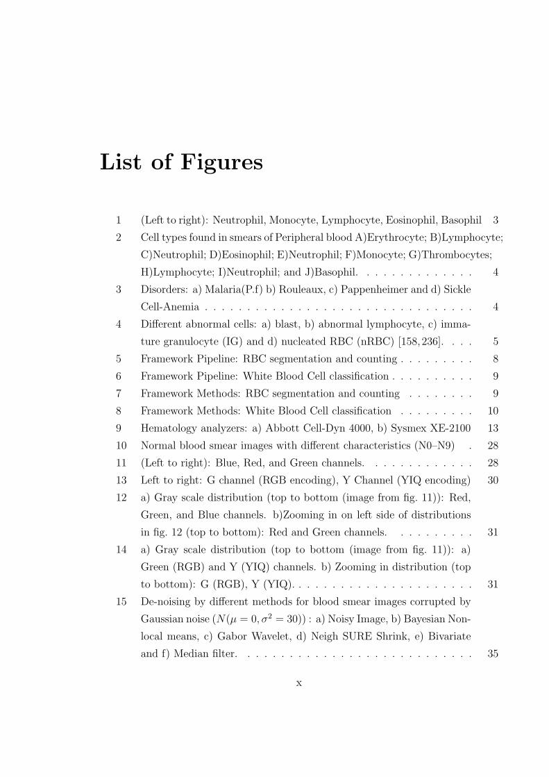
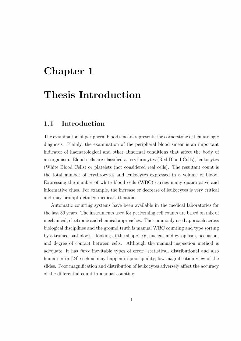
1 (Left to right): Neutrophil, Monocyte, Lymphocyte, Eosinophil, Basophil 3
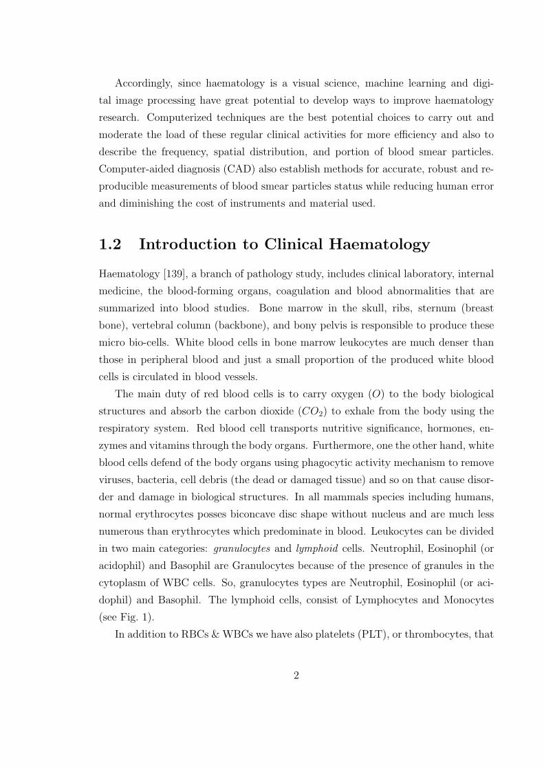
2 Cell types found in smears of Peripheral blood A)Erythrocyte; B)Lymphocyte;
C)Neutrophil; D)Eosinophil; E)Neutrophil; F)Monocyte; G)Thrombocytes;
H)Lymphocyte; I)Neutrophil; and J)Basophil. . . . . . . . . . . . . . 4
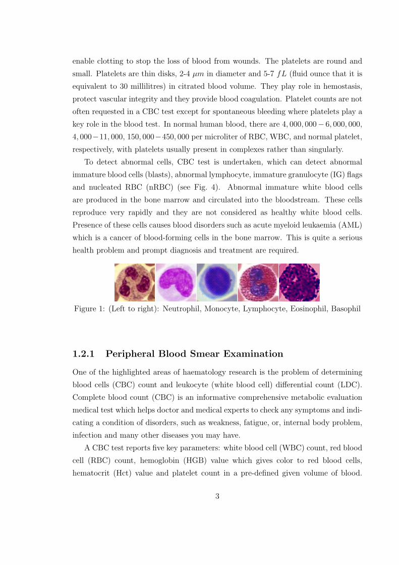
3 Disorders: a) Malaria(P.f) b) Rouleaux, c) Pappenheimer and d) Sickle
Cell-Anemia . . . . . . . . . . . . . . . . . . . . . . . . . . . . . . . . 4
4 Different abnormal cells: a) blast, b) abnormal lymphocyte, c) imma-
ture granulocyte (IG) and d) nucleated RBC (nRBC) [158,236]. . . . 5
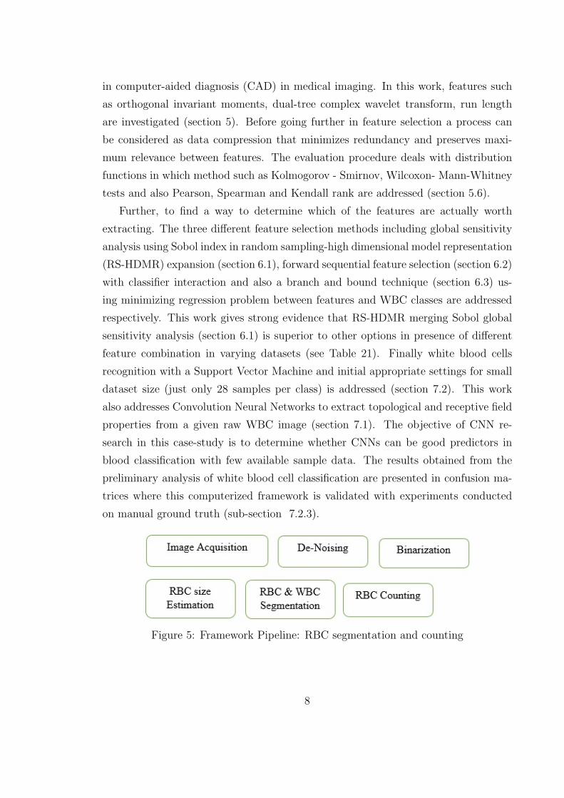
5 Framework Pipeline: RBC segmentation and counting . . . . . . . . . 8
6 Framework Pipeline: White Blood Cell classification . . . . . . . . . . 9
7 Framework Methods: RBC segmentation and counting . . . . . . . . 9
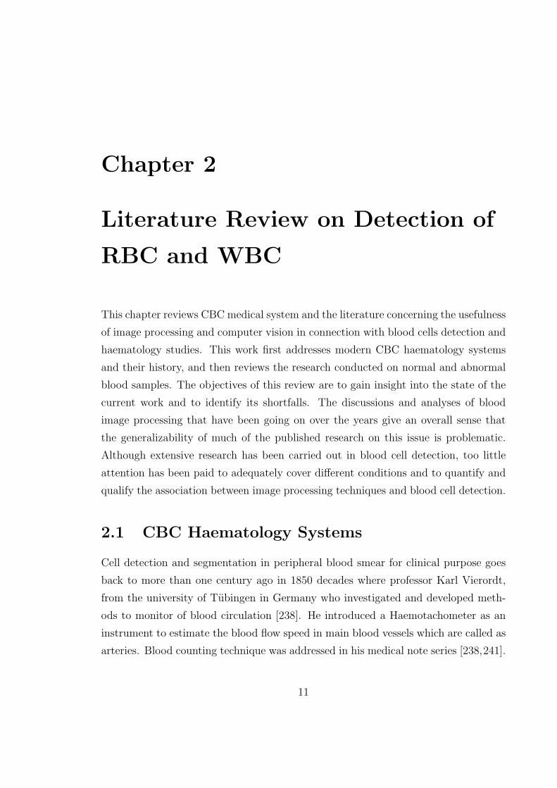
8 Framework Methods: White Blood Cell classification . . . . . . . . . 10
9 Hematology analyzers: a) Abbott Cell-Dyn 4000, b) Sysmex XE-2100 13
10 Normal blood smear images with different characteristics (N0–N9) . 28
11 (Left to right): Blue, Red, and Green channels. . . . . . . . . . . . . 28
13 Left to right: G channel (RGB encoding), Y Channel (YIQ encoding) 30
12 a) Gray scale distribution (top to bottom (image from fig. 11)): Red,
Green, and Blue channels. b)Zooming in on left side of distributions
in fig. 12 (top to bottom): Red and Green channels. . . . . . . . . . 31
14 a) Gray scale distribution (top to bottom (image from fig. 11)): a)
Green (RGB) and Y (YIQ) channels. b) Zooming in distribution (top
to bottom): G (RGB), Y (YIQ). . . . . . . . . . . . . . . . . . . . . . 31
15 De-noising by different methods for blood smear images corrupted by
Gaussian noise (N(µ = 0, σ2 = 30)) : a) Noisy Image, b) Bayesian Non-
local means, c) Gabor Wavelet, d) Neigh SURE Shrink, e) Bivariate
and f) Median filter. . . . . . . . . . . . . . . . . . . . . . . . . . . . 35
x
16 Edge-preserving for a given white blood cell image: a) Original b) Con-
volution kernel, c) Symmetrical Nearest Neighbour filter, d) Bilateral
filter and e) Kuwahara filter. . . . . . . . . . . . . . . . . . . . . . . . 35
17 Binarization methods: a) Bernsen; b) Sauvola; c) Otsu; and d) Niblack 49
18 Local Binarization Methods: a)Bradley b)Feng and c)Wolf . . . . . . 50
19 Binarization for low quality image: a, d) Original images b, e) Otsu,
c, f) Niblack . . . . . . . . . . . . . . . . . . . . . . . . . . . . . . . . 50
20 Granulometry over simple circle . . . . . . . . . . . . . . . . . . . . . 53
21 Patches and holes inside the RBC image . . . . . . . . . . . . . . . . 54
22 (Top to Bottom) a normal blood sample; an abnormal blood smear
sample (size detector) . . . . . . . . . . . . . . . . . . . . . . . . . . . 55
23 (left to right): a) de-noised green channel of initial sample; b) Granu-
lometry over blood smear sample (RBC size detector) . . . . . . . . . 56
24 Extracting a sub-image containing individual closed WBC regions: a,
b) Sub-images containing WBCs; c) Canny over Chan-Vese Active
Contour Without an Edge; d) Adding new edged image and enhanced
filled object; e) Modified filled object (closing SE=1px) . . . . . . . . 58
25 Separating WBCs from RBCs: a) WBC indicator; b) Separated RBC
sub-image . . . . . . . . . . . . . . . . . . . . . . . . . . . . . . . . . 59
26 Separating WBCs from RBCs: a) Sample slide; b) RBC separated
using this work ; c) Area- Opening [46] . . . . . . . . . . . . . . . . . 60
27 Separating WBCs from RBCs: a) Low quality sample ; b) WBC sepa-
rated using active contour [80,156,160]; c) WBC separated using Active
contours without edges [29]. . . . . . . . . . . . . . . . . . . . . . . . 60
28 Watershed marker over blood smear image . . . . . . . . . . . . . . . 61
29 Watershed for RBC counting: a) Solid RBCs; b) Watershed markers . 62
30 Q-shift DT-CWT [104], giving real and imaginary parts of complex
coefficients from two trees(α,β). The approximate delay for each filter
is shown by brackets in figures, where q = 1/4 sample period. . . . . . 87
31 LeNet-5 structure in modelling CNN for a 28×28 input image . . . 118
32 WBC testing data, each row, top to bottom: Basophil(B), Lympho-
cyte(L), Monocyte(M), Neutrophil(N), and Eosinophil(E). . . . . . . 122
33 Glossary of human blood smear terms . . . . . . . . . . . . . . . . . 135
xi
34 Normal blood smear images with different characteristics (N0–N5) . 136
35 Normal blood smear images with different characteristics (N6–N9) . . 137
36 Red Blood Cell Disorders: a)Malaria(P.f) b)Pappenheimer c)Sickle
Cell, d)Rouleaux . . . . . . . . . . . . . . . . . . . . . . . . . . . . . 138
37 Samples of white blood cells : a)Basophils b)Eosinophil c)Lymphocyte
d)Monocyte and e)Neutrophil (8 samples for each in different actual
size) . . . . . . . . . . . . . . . . . . . . . . . . . . . . . . . . . . . . 139
xii
List of Tables
1 Abbott Cell-Dyn 4000: Generic specifications and availability [69] . . 14
2 Sysmex XE-2100 Specifications . . . . . . . . . . . . . . . . . . . . . 14
3 Percentile range for different color map in different conditions: (top
to down: a, b, c); a) total over 10 regular images (N0–N9, whose
characteristics are described in figure 10); b) total over same 10 images
with moderate noise and c) same 10 images with high noise . . . . . . 29
4 Percentile range for Y (YIQ) and G (RGB) color map in different
conditions: (top to down: a, b, c); a) total over 10 regular images
(N0–N9, whose characteristics are described in figure 10); b) total over
same 10 images with moderate noise and c) same 10 images with high
noise . . . . . . . . . . . . . . . . . . . . . . . . . . . . . . . . . . . . 30
5 Variance of individual color channels (RGB color space) over 10 blood
smear images with different noise characteristics. . . . . . . . . . . . . 31
6 Variance of G (RGB color space) and Y (YIQ color space) over 10
blood smear images with different noise characteristics. . . . . . . . . 32
7 Non-linear de-noising techniques for blood smear samples using PSNR
levels with moderate and high Gaussian noise (N(µ = 0, σ2 = 30, 100)). 34
8 De-noising: Settings and Parametrization . . . . . . . . . . . . . . . . 37
9 Summary of normalized cross-correlation (NCC) data for each bina-
rization algorithm performance in different conditions: (top to bottom)
total over 10 regular images (N0–N9); . . . . . . . . . . . . . . . . . 63
xiii
10 Summary of normalized cross-correlation (NCC) data for each bina-
rization algorithm performance in different conditions for sample sep-
arated WBCs: (top to bottom) total over 10 regular images (N0–N9);
total over 10 moderate Gaussian Noise; 10 images with high Gaus-
sian Noise; total over 10 moderate Speckle Noise; 10 images with high
Speckle Noise; total over 10 regular blurry images (N0–N9) . . . . . . 64
11 Summary of normalized cross-correlation (NCC) data for each binariza-
tion algorithm performance in different conditions for windows sample
including few disjoint close by RBCs: (top to bottom) total over 10
regular images (N0–N9); total over 10 moderate Gaussian Noise; 10 im-
ages with high Gaussian Noise; total over 10 moderate Speckle Noise;
10 images with high Speckle Noise; total over 10 regular blurry images
(N0–N9) . . . . . . . . . . . . . . . . . . . . . . . . . . . . . . . . . . 65
12 Boundaries detection: Settings . . . . . . . . . . . . . . . . . . . . . . 66
13 Experimental results of ten different blood smear images (numbered
N0 – N9). Counts for RBCs and WBCs are given from manual counts,
as well as by our framework using either Bivariate, or Gabor Wavelet.
Values given in parentheses are the differences between counts com-
puted and those obtained by a manual count (negative values indicate
under-count; positive values indicate over-count). The last column
labelled Subtypes refers to the WBC subtypes. In addition, the re-
sults are compared to those of the work [18,44,46] and their extended
work [224,225,226]. . . . . . . . . . . . . . . . . . . . . . . . . . . . . 67
14 Comparative Study of Invariant Moment Approaches . . . . . . . . . 83
15 Orthogonal Invariant Moments: Setting . . . . . . . . . . . . . . . . . 88
16 P-values for Kolmogorov-Smirnov test, totals over 11 moment series
(see Section 5.3.2), different feature sets. . . . . . . . . . . . . . . . . 96
17 P-values for Mann-Whitney test, totals over 11 moment series (see. 5.3.2),
different feature sets. . . . . . . . . . . . . . . . . . . . . . . . . . . . 97
18 Correlation degree for Pearson test, totals over 11 moment series (see. 5.3.2),
different feature sets. . . . . . . . . . . . . . . . . . . . . . . . . . . . 100
19 Correlation degree for Spearman test, totals over 11 moment series(see. 5.3.2),
different feature sets. . . . . . . . . . . . . . . . . . . . . . . . . . . . 101
xiv
20 The first five shifted Legendre polynomial terms . . . . . . . . . . . . 106
21 Global sensitivity analysis (top to down: a, b) for RS-HDMR expan-
sion, in connection with total features over each white blood cell image 115
22 Confusion matrices for CNN, total over testing images . . . . . . . . 119
23 Confusion matrices for Linear SVM with feature set dimensionality
reduction using K-PCA, total over testing images . . . . . . . . . . . 119
24 Confusion matrices for Linear SVM without dimension reduction, total
over testing images . . . . . . . . . . . . . . . . . . . . . . . . . . . . 119
25 Confusion matrices (top to down: a,b,c,d) for SVM classifier, totals
over testing images in invariant features & linear SVM . . . . . . . . 125
26 Support Vector Machine: Settings . . . . . . . . . . . . . . . . . . . . 126
27 Convolutional neural network: Settings . . . . . . . . . . . . . . . . . 126
xv
Chapter 1
Thesis Introduction
1.1 Introduction
The examination of peripheral blood smears represents the cornerstone of hematologic
diagnosis. Plainly, the examination of the peripheral blood smear is an important
indicator of haematological and other abnormal conditions that affect the body of
an organism. Blood cells are classified as erythrocytes (Red Blood Cells), leukocytes
(White Blood Cells) or platelets (not considered real cells). The resultant count is
the total number of erythrocytes and leukocytes expressed in a volume of blood.
Expressing the number of white blood cells (WBC) carries many quantitative and
informative clues. For example, the increase or decrease of leukocytes is very critical
and may prompt detailed medical attention.
Automatic counting systems have been available in the medical laboratories for
the last 30 years. The instruments used for performing cell counts are based on mix of
mechanical, electronic and chemical approaches. The commonly used approach across
biological disciplines and the ground truth is manual WBC counting and type sorting
by a trained pathologist, looking at the shape, e.g, nucleus and cytoplasm, occlusion,
and degree of contact between cells. Although the manual inspection method is
adequate, it has three inevitable types of error: statistical, distributional and also
human error [24] such as may happen in poor quality, low magnification view of the
slides. Poor magnification and distribution of leukocytes adversely affect the accuracy
of the differential count in manual counting.
1
Accordingly, since haematology is a visual science, machine learning and digi-
tal image processing have great potential to develop ways to improve haematology
research. Computerized techniques are the best potential choices to carry out and
moderate the load of these regular clinical activities for more efficiency and also to
describe the frequency, spatial distribution, and portion of blood smear particles.
Computer-aided diagnosis (CAD) also establish methods for accurate, robust and re-
producible measurements of blood smear particles status while reducing human error
and diminishing the cost of instruments and material used.
1.2 Introduction to Clinical Haematology
Haematology [139], a branch of pathology study, includes clinical laboratory, internal
medicine, the blood-forming organs, coagulation and blood abnormalities that are
summarized into blood studies. Bone marrow in the skull, ribs, sternum (breast
bone), vertebral column (backbone), and bony pelvis is responsible to produce these
micro bio-cells. White blood cells in bone marrow leukocytes are much denser than
those in peripheral blood and just a small proportion of the produced white blood
cells is circulated in blood vessels.
The main duty of red blood cells is to carry oxygen (O) to the body biological
structures and absorb the carbon dioxide (CO2) to exhale from the body using the
respiratory system. Red blood cell transports nutritive significance, hormones, en-
zymes and vitamins through the body organs. Furthermore, one the other hand, white
blood cells defend of the body organs using phagocytic activity mechanism to remove
viruses, bacteria, cell debris (the dead or damaged tissue) and so on that cause disor-
der and damage in biological structures. In all mammals species including humans,
normal erythrocytes posses biconcave disc shape without nucleus and are much less
numerous than erythrocytes which predominate in blood. Leukocytes can be divided
in two main categories: granulocytes and lymphoid cells. Neutrophil, Eosinophil (or
acidophil) and Basophil are Granulocytes because of the presence of granules in the
cytoplasm of WBC cells. So, granulocytes types are Neutrophil, Eosinophil (or aci-
dophil) and Basophil. The lymphoid cells, consist of Lymphocytes and Monocytes
(see Fig. 1).
In addition to RBCs & WBCs we have also platelets (PLT), or thrombocytes, that
2
enable clotting to stop the loss of blood from wounds. The platelets are round and
small. Platelets are thin disks, 2-4 µm in diameter and 5-7 fL (fluid ounce that it is
equivalent to 30 millilitres) in citrated blood volume. They play role in hemostasis,
protect vascular integrity and they provide blood coagulation. Platelet counts are not
often requested in a CBC test except for spontaneous bleeding where platelets play a
key role in the blood test. In normal human blood, there are 4, 000, 000− 6, 000, 000,
4, 000−11, 000, 150, 000−450, 000 per microliter of RBC, WBC, and normal platelet,
respectively, with platelets usually present in complexes rather than singularly.
To detect abnormal cells, CBC test is undertaken, which can detect abnormal
immature blood cells (blasts), abnormal lymphocyte, immature granulocyte (IG) flags
and nucleated RBC (nRBC) (see Fig. 4). Abnormal immature white blood cells
are produced in the bone marrow and circulated into the bloodstream. These cells
reproduce very rapidly and they are not considered as healthy white blood cells.
Presence of these cells causes blood disorders such as acute myeloid leukaemia (AML)
which is a cancer of blood-forming cells in the bone marrow. This is quite a serious
health problem and prompt diagnosis and treatment are required.
Figure 1: (Left to right): Neutrophil, Monocyte, Lymphocyte, Eosinophil, Basophil
1.2.1 Peripheral Blood Smear Examination
One of the highlighted areas of haematology research is the problem of determining
blood cells (CBC) count and leukocyte (white blood cell) differential count (LDC).
Complete blood count (CBC) is an informative comprehensive metabolic evaluation
medical test which helps doctor and medical experts to check any symptoms and indi-
cating a condition of disorders, such as weakness, fatigue, or, internal body problem,
infection and many other diseases you may have.
A CBC test reports five key parameters: white blood cell (WBC) count, red blood
cell (RBC) count, hemoglobin (HGB) value which gives color to red blood cells,
hematocrit (Hct) value and platelet count in a pre-defined given volume of blood.
3
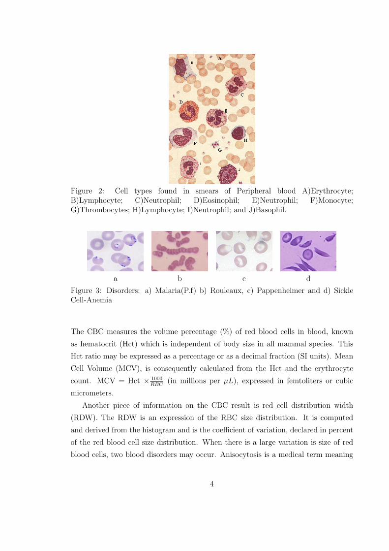
Figure 2: Cell types found in smears of Peripheral blood A)Erythrocyte;B)Lymphocyte; C)Neutrophil; D)Eosinophil; E)Neutrophil; F)Monocyte;G)Thrombocytes; H)Lymphocyte; I)Neutrophil; and J)Basophil.
a b c d
Figure 3: Disorders: a) Malaria(P.f) b) Rouleaux, c) Pappenheimer and d) SickleCell-Anemia
The CBC measures the volume percentage (%) of red blood cells in blood, known
as hematocrit (Hct) which is independent of body size in all mammal species. This
Hct ratio may be expressed as a percentage or as a decimal fraction (SI units). Mean
Cell Volume (MCV), is consequently calculated from the Hct and the erythrocyte
count. MCV = Hct × 1000RBC
(in millions per µL), expressed in femtoliters or cubic
micrometers.
Another piece of information on the CBC result is red cell distribution width
(RDW). The RDW is an expression of the RBC size distribution. It is computed
and derived from the histogram and is the coefficient of variation, declared in percent
of the red blood cell size distribution. When there is a large variation is size of red
blood cells, two blood disorders may occur. Anisocytosis is a medical term meaning
4
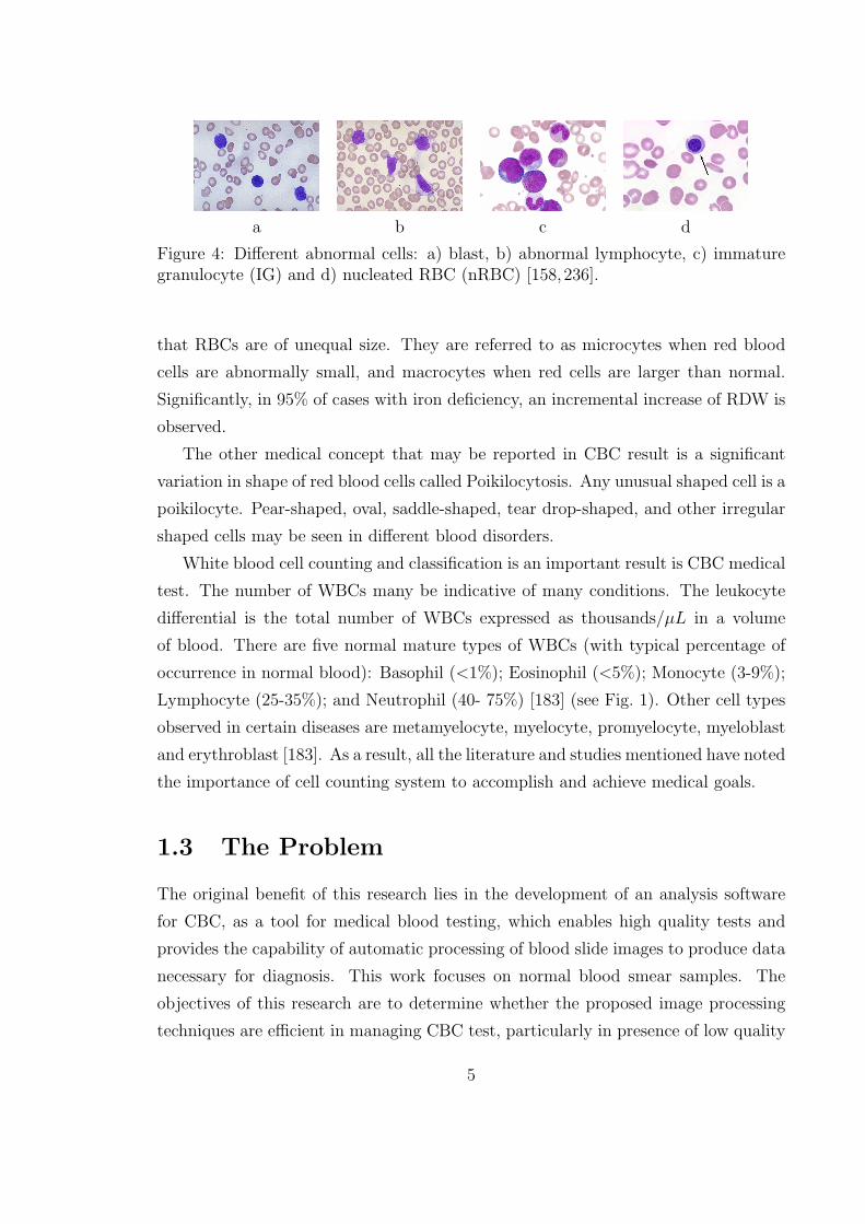
a b c d
Figure 4: Different abnormal cells: a) blast, b) abnormal lymphocyte, c) immaturegranulocyte (IG) and d) nucleated RBC (nRBC) [158,236].
that RBCs are of unequal size. They are referred to as microcytes when red blood
cells are abnormally small, and macrocytes when red cells are larger than normal.
Significantly, in 95% of cases with iron deficiency, an incremental increase of RDW is
observed.
The other medical concept that may be reported in CBC result is a significant
variation in shape of red blood cells called Poikilocytosis. Any unusual shaped cell is a
poikilocyte. Pear-shaped, oval, saddle-shaped, tear drop-shaped, and other irregular
shaped cells may be seen in different blood disorders.
White blood cell counting and classification is an important result is CBC medical
test. The number of WBCs many be indicative of many conditions. The leukocyte
differential is the total number of WBCs expressed as thousands/µL in a volume
of blood. There are five normal mature types of WBCs (with typical percentage of
occurrence in normal blood): Basophil (<1%); Eosinophil (<5%); Monocyte (3-9%);
Lymphocyte (25-35%); and Neutrophil (40- 75%) [183] (see Fig. 1). Other cell types
observed in certain diseases are metamyelocyte, myelocyte, promyelocyte, myeloblast
and erythroblast [183]. As a result, all the literature and studies mentioned have noted
the importance of cell counting system to accomplish and achieve medical goals.
1.3 The Problem
The original benefit of this research lies in the development of an analysis software
for CBC, as a tool for medical blood testing, which enables high quality tests and
provides the capability of automatic processing of blood slide images to produce data
necessary for diagnosis. This work focuses on normal blood smear samples. The
objectives of this research are to determine whether the proposed image processing
techniques are efficient in managing CBC test, particularly in presence of low quality
5
samples. We particularly interested in the classification of the five main types of
white blood cells (leukocytes) and counting of normal red blood cells (erythrocytes)
in a clinical setting.
For many medical topics, studies usually suffer from the fact that it is not easy
to access large amounts of samples. Blood samples in this work were obtained from
normal healthy patients. A total of 140 samples were obtained in cooperation with
J.D. MacLean Centre for Tropical Diseases at McGill University in Montreal, Quebec
and also Ghods polyclinic medical center in Tehran, Iran. All samples are validated by
MD Hematologist Doctor, Parvaneh Saberian and medical specialist, microbiologist,
Aida Habibzadeh from Ghods polyclinic medical center in Tehran, Iran. Despite a
small sample size, the dataset is generally representative of different conditions that
may exist in a blood smear.
1.4 Thesis Structure
We discuss implementations of color conversion, de-noising, edge preserving and
counting red blood cells as well as white blood cell classification. This work begins
by laying out the theoretical dimensions of the research, and looks at how each step
is involved in framework. Chapters describe the design, synthesis, characterization
and evaluation of all details. The performance of proposed method is also compared
with the state-of-the-art work.
The framework begins with interpretation of the peripheral blood smear (chapter
1, section 1.2. Next, this work gives a comprehensive overview of the recent history of
red and white blood cell classification where each has its advantages and drawbacks.
Background information were gathered from multiple sources between 1972 and 2014
(chapter 2). Chapters (3 - 7) begin by laying out the theoretical dimensions of the
research step, and looks at how these methods are good at the complete blood count
(CBC) results and interpretation. It describes the design, synthesis, characterization
and evaluation of proposed framework. The section 8.1, in chapter 8 summarizes novel
contributions of this thesis in the area of normal blood segmentation and classification.
Also all parameters that should be manually set for each component are clarified in
individual final section in each step. This clarification gives the reader a clear idea
how this framework and could be applied successfully to a different data set. Chapter
6
8 includes conclusion and suggestion for future work. Some blood smear samples in
different conditions are shown in the appendix (chapter 9).
This thesis made research contributions in five areas: pre-processing, binarization,
cell separation, and feature extraction, and finally feature selection and classification.
Figures 5 and 6 demonstrate pipeline of the framework indicating what is the
step used for each part. Figures 7 and 8 indicate the methodology used in each part.
1.4.1 Methodologies Used
On continuing discussion concerning the methodologies used (see Figures 7 and 8),
the normal blood images are saved in JPEG format. Then a key step is to choose a
proper gray scale channel to maintain the high and low frequency of components in
a given blood image and white blood cells with special characteristics in particular.
Distribution behaviours statistical approaches such as semi-IQR and variance are ad-
dressed to convert the blood smear images to a proper gray scale . In current dataset
G channel rather than the other channels is selected (section 3.1). It also should
be noted that other combination of channels such as Y and G might be even result
better in Semi-IQR calculation and future work by other researcher could investigate
in this matter. Secondly, the method used for denoising is based on the Bayesian non
local mean. In a comparative study with other state-of-the art work Bayesian non
local mean brings the highest PSNR value in presence of additive Gaussian noise (see
Table 7). Thirdly, to build better boundaries for white blood cells and also to replace
white blood cell internal heterogeneous parts by homogeneous neighbours, Kuwahara
filter is addressed (see Fig. 16). Then, a binarization technique is introduced by
merging the Otsu and Niblack methods (section 4). Area-Granulometry is used to
estimate RBC size (see Fig. 23). Afterwards, the proposed Cell separation algorithm
in an iterative mechanism based on morphological theory, saturation amount, RBC
size, edged images and modified Chan-Vese active contours without edges is applied
(section 4.3.3). A primary aim of this work is to introduce an accurate mechanism
for RBCs counting. This is accomplished by using the immersion-based watershed
algorithm which counts red cells separately (section 4.3.4). Next, white blood cells
(leukocytes) classification into five major categories using invariant features such as
shape, intensity and texture is addressed. Although diverse algorithms have been de-
veloped using well established mathematical theory, it remains comparably marginal
7
in computer-aided diagnosis (CAD) in medical imaging. In this work, features such
as orthogonal invariant moments, dual-tree complex wavelet transform, run length
are investigated (section 5). Before going further in feature selection a process can
be considered as data compression that minimizes redundancy and preserves maxi-
mum relevance between features. The evaluation procedure deals with distribution
functions in which method such as Kolmogorov - Smirnov, Wilcoxon- Mann-Whitney
tests and also Pearson, Spearman and Kendall rank are addressed (section 5.6).
Further, to find a way to determine which of the features are actually worth
extracting. The three different feature selection methods including global sensitivity
analysis using Sobol index in random sampling-high dimensional model representation
(RS-HDMR) expansion (section 6.1), forward sequential feature selection (section 6.2)
with classifier interaction and also a branch and bound technique (section 6.3) us-
ing minimizing regression problem between features and WBC classes are addressed
respectively. This work gives strong evidence that RS-HDMR merging Sobol global
sensitivity analysis (section 6.1) is superior to other options in presence of different
feature combination in varying datasets (see Table 21). Finally white blood cells
recognition with a Support Vector Machine and initial appropriate settings for small
dataset size (just only 28 samples per class) is addressed (section 7.2). This work
also addresses Convolution Neural Networks to extract topological and receptive field
properties from a given raw WBC image (section 7.1). The objective of CNN re-
search in this case-study is to determine whether CNNs can be good predictors in
blood classification with few available sample data. The results obtained from the
preliminary analysis of white blood cell classification are presented in confusion ma-
trices where this computerized framework is validated with experiments conducted
on manual ground truth (sub-section 7.2.3).
Figure 5: Framework Pipeline: RBC segmentation and counting
8
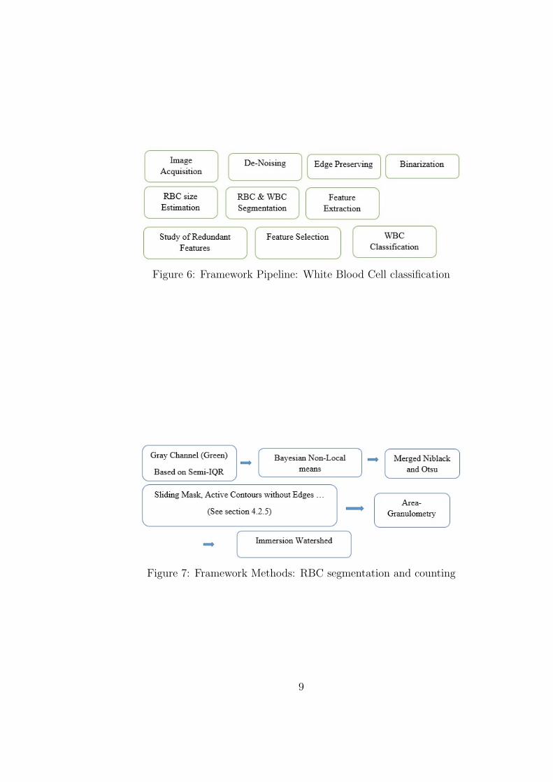
Figure 6: Framework Pipeline: White Blood Cell classification
Figure 7: Framework Methods: RBC segmentation and counting
9
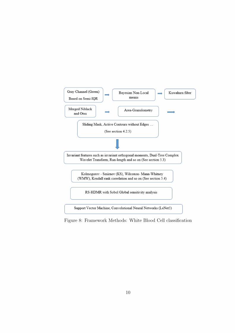
Figure 8: Framework Methods: White Blood Cell classification
10
Chapter 2
Literature Review on Detection of
RBC and WBC
This chapter reviews CBC medical system and the literature concerning the usefulness
of image processing and computer vision in connection with blood cells detection and
haematology studies. This work first addresses modern CBC haematology systems
and their history, and then reviews the research conducted on normal and abnormal
blood samples. The objectives of this review are to gain insight into the state of the
current work and to identify its shortfalls. The discussions and analyses of blood
image processing that have been going on over the years give an overall sense that
the generalizability of much of the published research on this issue is problematic.
Although extensive research has been carried out in blood cell detection, too little
attention has been paid to adequately cover different conditions and to quantify and
qualify the association between image processing techniques and blood cell detection.
2.1 CBC Haematology Systems
Cell detection and segmentation in peripheral blood smear for clinical purpose goes
back to more than one century ago in 1850 decades where professor Karl Vierordt,
from the university of Tubingen in Germany who investigated and developed meth-
ods to monitor of blood circulation [238]. He introduced a Haemotachometer as an
instrument to estimate the blood flow speed in main blood vessels which are called as
arteries. Blood counting technique was addressed in his medical note series [238,241].
11
Briefly, this research served as the base for future studies where obviously Vierordt
work and findings added substantially to our understanding of blood circulation and
haematology basic.
The design of the counting blood cells further developed based on research work by
Cramer [37,238], Potain and Malassez and the other [134] in the middle 19th century.
The research during the late 19th and early 20th century from different studies by
Hayem [85] as a known French hematologist, and also the technique introduced by
Oliver [159] an English physician made several contributions to the current literature.
A rapid change is made in the twenties, as a result of the development in pho-
toelectric methods. During years, different electronic counting systems with flow of
electrical current and based on conduction were introduced [238]. Since the last 25
years automatic counting system have been available in the medical laboratories with
the less and more similar structure [24]. The instruments used to perform cell counts
are based on mix of mechanical, electronic and chemical approaches. They are made
on the principles of electrical impedance, radio-frequency conductivity, light scatter-
ing, and/or cytochemistry. With electrical impedance, blood cells passing through an
valve and aperture which a current is flowing cause changes in electrical resistance to
provide voltage pulses. In an updated electrical impedance technique red blood cell
size distributions automatically will be plotted. In radio-frequency conductivity tech-
nique, using a high-frequency electromagnetic probe information on the cell internal
structure will be provided by spreading or flowing throughout the fat layer of a blood
cells membrane. In the electro-optical method, size of the particle (WBC, RBC, or
platelet) is determined by light scattering. Forward angle scatter of a light determines
cell surface characteristics and measurement of beam scatter at multiple light angles
to differentiate of cell types. In cytochemistry analysis, cytochemical reaction used to
detect white blood cells. This method usually works along with electro-optical and
data derived from light scattered to aid white blood cell differentiation [24].
2.1.1 Current CBC Systems
Current hematology analyzers used routinely in modern medical laboratories are such
as Sysmex XE-series [197] and also Abbott CELL-DYN [69]. The Abbott Cell-Dyn
4000 hematology analyzer integrates four measurement sub-system to accomplish
almost a complete CBC medical test. This system works with fluorescence flow
12
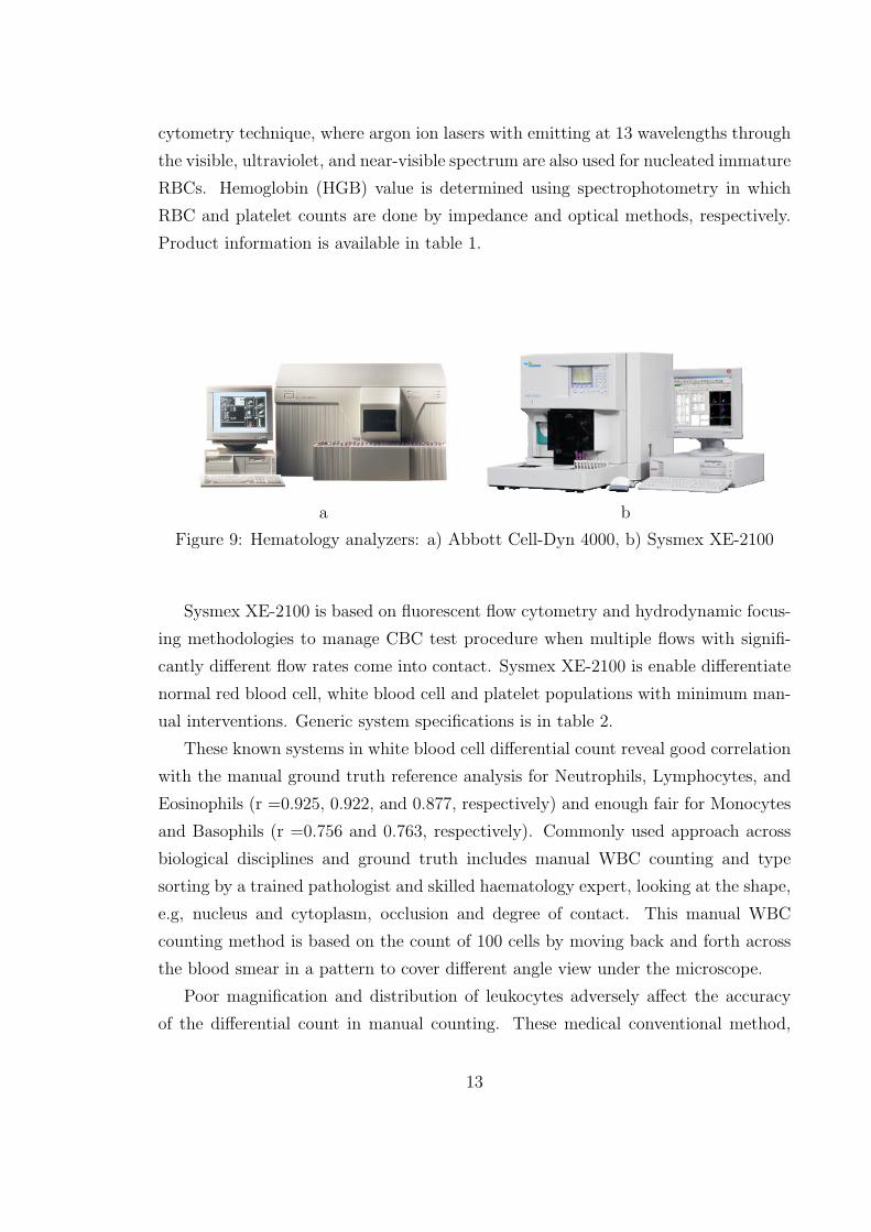
cytometry technique, where argon ion lasers with emitting at 13 wavelengths through
the visible, ultraviolet, and near-visible spectrum are also used for nucleated immature
RBCs. Hemoglobin (HGB) value is determined using spectrophotometry in which
RBC and platelet counts are done by impedance and optical methods, respectively.
Product information is available in table 1.
a b
Figure 9: Hematology analyzers: a) Abbott Cell-Dyn 4000, b) Sysmex XE-2100
Sysmex XE-2100 is based on fluorescent flow cytometry and hydrodynamic focus-
ing methodologies to manage CBC test procedure when multiple flows with signifi-
cantly different flow rates come into contact. Sysmex XE-2100 is enable differentiate
normal red blood cell, white blood cell and platelet populations with minimum man-
ual interventions. Generic system specifications is in table 2.
These known systems in white blood cell differential count reveal good correlation
with the manual ground truth reference analysis for Neutrophils, Lymphocytes, and
Eosinophils (r =0.925, 0.922, and 0.877, respectively) and enough fair for Monocytes
and Basophils (r =0.756 and 0.763, respectively). Commonly used approach across
biological disciplines and ground truth includes manual WBC counting and type
sorting by a trained pathologist and skilled haematology expert, looking at the shape,
e.g, nucleus and cytoplasm, occlusion and degree of contact. This manual WBC
counting method is based on the count of 100 cells by moving back and forth across
the blood smear in a pattern to cover different angle view under the microscope.
Poor magnification and distribution of leukocytes adversely affect the accuracy
of the differential count in manual counting. These medical conventional method,
13
therefore, suffer from imprecision, and poor clinical setting. In other hand, the ery-
throcytes and leukocyte types that the current equipments are able to manage are
restricted to some classes where always update of these systems are based on expensive
chemicals and mechanical process [175]. As mentioned, the microscope inspection of
blood slides provides important qualitative and quantitative information concerning
the presence of hematic pathologies [173], however the number of different sub-cell
types that can come out especially for WBC count is relatively large and typically
more than 20 [175]. A systematic method and meticulous technique to derive all
accurate and consistent cell information from each blood smear examine is highly
required. These comprehensive blood studies increase the difficulty in building a
feasible hardware based system. Overall, it can be seen that the majority of blood
diseases can be detected using image processing and computer vision techniques.
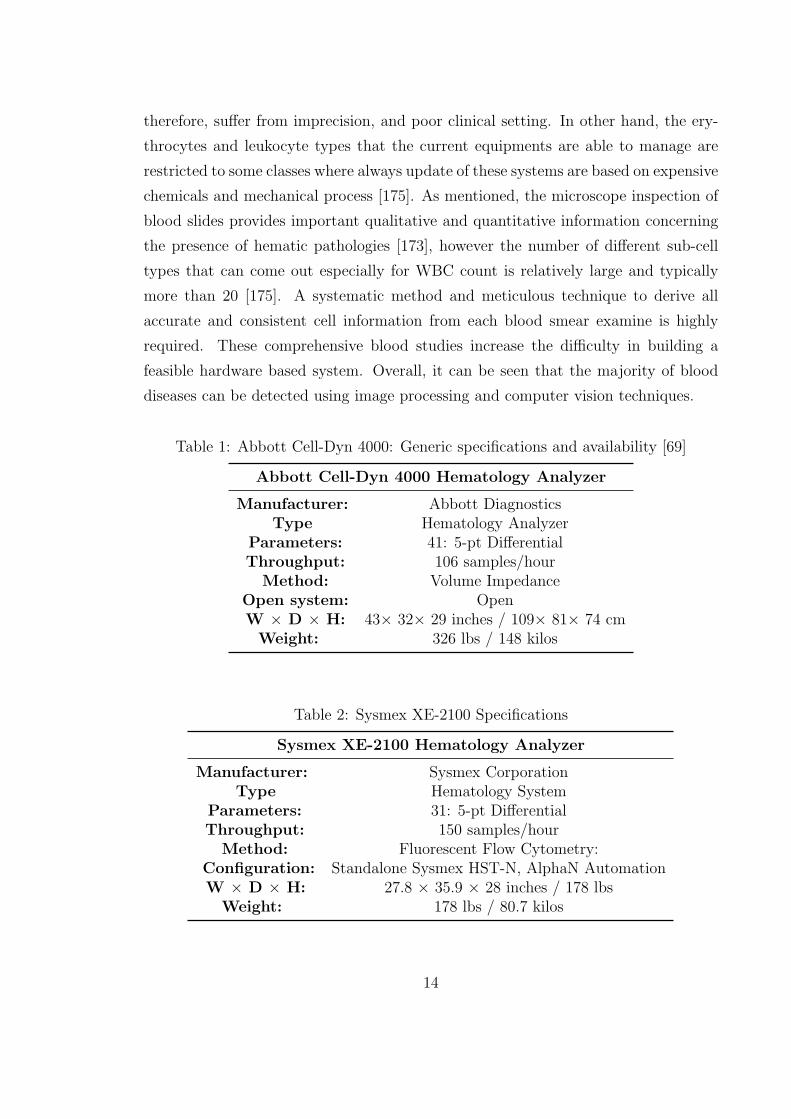
Table 1: Abbott Cell-Dyn 4000: Generic specifications and availability [69]
Abbott Cell-Dyn 4000 Hematology Analyzer
Manufacturer: Abbott DiagnosticsType Hematology Analyzer
Parameters: 41: 5-pt DifferentialThroughput: 106 samples/hour
Method: Volume ImpedanceOpen system: OpenW × D × H: 43× 32× 29 inches / 109× 81× 74 cm
Weight: 326 lbs / 148 kilos
Table 2: Sysmex XE-2100 Specifications
Sysmex XE-2100 Hematology Analyzer
Manufacturer: Sysmex CorporationType Hematology System
Parameters: 31: 5-pt DifferentialThroughput: 150 samples/hour
Method: Fluorescent Flow Cytometry:Configuration: Standalone Sysmex HST-N, AlphaN AutomationW × D × H: 27.8 × 35.9 × 28 inches / 178 lbs
Weight: 178 lbs / 80.7 kilos
14
2.2 The Literature on Image Processing in CBC
CBC process can be automated by computerized techniques which are more reliable
and economic. Therefore there is always a need for the development of systems to pro-
vide assistance to haematologists and to relieve the physician of drudgery or repetitive
work. Computer-aided diagnosis (CAD) will establish methods for precise, accurate,
robust and reproducible measurements of blood smear particles status while reducing
human error and diminish the cost of instruments and material used. Afterwards,
software provides the capabilities of upgrading and measurement variability without
major changes and extra burdens.
The computerized steps into automated blood examination refers to a work done
by Bentley and Lewis [14] in 1975. In this early work, authors used of colour in-
formation analysis to obtain integrated data on erythrocytes size in a numbers of
normal and abnormal red blood cells. This paper went after to address the correla-
tion between MCV (mean corpuscular volume) refers to the size of erythrocyte and
MCH (mean corpuscular hemoglobin) refers to the concentration of hemoglobin in
red blood cells. One decade after, the first fully automated processing of blood smear
slides was introduced by Rowan [195] in 1986. Further related references are listed in
below sections.
2.2.1 Literature Review on Segmentation
Initial success on segmentation of medical imaging and blood segmentation was ob-
tained with graph theory (Martelli [138], Osowski et al. [163], Fleagle et al. [58, 59])
which was used to navigate around edge pixels in an available image. However this
approach has involved images of single objects manually located in an image. Fur-
ther, it does not address the problems of multiple objects in the image. Therefore,
object location, removal of extraneous edges (internal to the cell), or the selection of
suitable starting and ending points for the graph search are the initial steps which
are should considered. These arguments rely too heavily on quantitative analysis of
manual aforementioned pre-processing steps where it is always an inconsistency with
this argument. There is no consensus among researchers regarding what method can
be applied for different conditions, and there is no general agreement about these
initial steps.
15
Due to complexity of the problem at hand some of the papers are limited to
image-based comparisons based on red cells segmented either manually, see Bentley
& Lewis [14], Albertini et al. [3], or semi-automatically, see Robinson et al. [192],
Costin et al. [35] and Gering & Atkinson [66]. Dong et al. [48] proposed a frame-
work with three steps to identify rolling leukocytes in microscopic images. This work
profits gradient inverse coefficients of variation (GICOV) to discriminate leukocytes
in-vivo environment. Authors first build a set of arbitrary number of ellipses by vary-
ing radii and orientation. Local maximum in gradient inverse coefficients of varying
value denote presence of white blood cell in a close-by ellipse area where ellipses cor-
responding to locally maximum GICOV will be relaxed to flexible contours by active
B-spline curves. Rathore et al. [184] used a method to estimate circularity ratio of
cells. Counting is also done using watershed segmentation and Pixcavator student
edition software. Lepcha et al. [122] segmented and counted number of red blood cells
using integration of marker controlled watershed segmentation and morphological op-
erations. Khajehpour et al. [71] introduced a line operator and watershed algorithm
to segment red blood cells. The line operator with 20 line segments in various di-
rections over a global Otsu threshold image has been applied. Wei et al. [246] first
employed a K-means classification to detect of leukocyte and then counting RBC was
addressed using watershed.
Literature Review on Thresholding
Adjouadi et al. [1] used eight-directional scanning to detect the red blood cell bound-
aries over the thresholded binarized input images. This work examined clustering-
based image thresholding to segment cells. One major criticism of Adjouadi’s work is
that it relies heavily on initial conditions in a given blood smear slide. It used global
thresholding and then the existing framework fails to resolve the thresholding prob-
lem in presence of different possible staining. There is no general agreement about
all possible cells.
2.2.2 Literature Review on White Blood Cell Detection
To go further in discussion and to interpret health changes accurately, practitioners
must get knowledge of a complete white blood cell five-part differential. The back-
ground on white blood cell classification using computer vision concepts is very vast
16
and it involves feature extractors, classifiers, quantitative and qualitative process,
e.g., [51, 183, 189, 208, 228]. The first paper on blood processing is leukocyte pattern
recognition by Bacusmber and Gose in 1972 [11]. In this primary work, classification
of white blood cells using shape features and a multivariate Gaussian classifier into
their categories are presented. In 1986, the first fully automated processing of blood
smear slides was introduced by Rowan [195] .
Active contour model background
Active contour model, or snake is an another common method of boundary detec-
tion [99]. In 2001, Ongun et al. published a paper [160,162] in which they described
how active contour models facilitate white blood cell edge and boundaries detection.
In other work [160], active contours were also used to track the boundaries of white
blood cell where occluded cells were not accurately handled. A computerized sys-
tem where cells are segmented using active contour models was introduced in [161]
using shape features and textures for classification. WBC classification in 2009 by
Hamghalam et al. [80] utilizes Otsu’s thresholding method to nuclei segmentation.
The results are claimed independent of the intensity differences in Giemsa-stained
images of peripheral blood smear and active contours are used to extract precise
boundary of cytoplasm but in simulation it failed in different condition. Mukherjee
et al. [148] proposed a leukocyte detection framework with image-level sets computed
via threshold decomposition. An evolution of a level-set curve that maximizes image
gradient along homogeneous region was considered as cell boundaries. In general,
despite active contour model efficacy in deformed cells, this method is not fully au-
tomatic. This method relies on initial positioning for snake algorithms and to date,
little evidence has been found associating active contour model with full automated
system. It is very obvious that with wrong initial model positioning, boundaries are
also tracked negatively.
Fuzzy logic background
Sobrevilla et al. [215] used fuzzy logic to segment white blood cells from a digital blood
smear image. In that proposed fuzzy logic two regions were segmented; one was the
interest region, which contained leukocytes and other part included stained back-
grounds with light gray level homogeneous texture, erythrocytes with light-medium
17
gray level and lastly, it also included the contours of white blood cells in correspon-
dence with heterogeneous areas. In this way both intensity level, homogeneity and
heterogeneity taken into account to distinguish between white blood cells and other
particles in digital image. However, in both TSMM [252] and fuzzy logic [215], pa-
rameter settings were needed to set by statistics and experience. Also, it was limited
to very obvious differences among backgrounds, red blood cells, and white blood cells
in correspondence with homogeneous areas. Hence, both frameworks fail in different
conditions such as color conversion and varying illumination staining inconsistency.
Afterwards, Shitong et al. [208] proposed white blood cell detection based on fuzzy
cellular neural networks (FCNN). FCNN is a hybrid system of fuzzy logic and neural
networks (NNs). Experimental results showed that the mentioned detailed approach
performance was more efficient than the other comparative methods in paper includ-
ing TSMM [252] and fuzzy logic approach [215]. This method [208] took advantage of
neural network classification and regression performance, combination of Neural Net-
work and fuzzy logic facilitated Classification in uncertain condition in cell pattern
recognition.
Morphological changes background
Lezoray [123] introduced region-based white blood cells segmentation using extracted
markers (or seeds). However, this method required prior knowledge of color infor-
mation for proper seed extraction. Kumar [114] applied a novel cell edge detector
while trying to perfectly determine the boundary of the nucleus. Furthermore, in
other work, WBC segmentation was achieved by means of mean-shift-based color
segmentation in Comaniciu and Meer research work [34] while in [95] Jiang et al.
used watershed segmentation. In other work, in order to improve the segmentation
of touching or adjacent blood cells, conventional and typical wavelet transformation
combined with morphological operations was proposed in Chan and his co-authors
work [28]. Yang et al. [255] used a combination of RGB and HSI to describe color
space in white blood cell. This work detect white blood cell with gathering color
information in Saturation (from HSI) and Blue (from RGB) channels.
18
Feature Extraction background
Ramoser et al. [183] used hue, saturation and luminance values to locate WBCs.
Then it goes on classification using a 26-dimensional color feature vector and a poly-
nomial support vector machine (SVM). However, this proposed framework [183] did
not address different conditions in camera settings, magnification, varying inconsis-
tent illumination and blood staining. It also ignored texture features that they may
produce appropriate space and proper meaningful output to object recognition due
to authors false assumption about size and texture feature computation. Xiao-min
et al. [252] introduced method based on threshold segmentation followed by math-
ematical morphology (TSMM). In that work binary threshold segmentation was in
the first step. The individual white blood cells were detected using the average gray
value of cytoplasm as the threshold and then binary segmentation was done; also it
was calibrated with erosion and dilation applied to the binary image, where number
of morphological operations was assigned by experience. Following that, the WBC
nuclei was located with the shape features in correspondence with area and roundness.
Bikhet et al. [18] used 10 features from cytoplasm region to classify five main white
blood cell types. This work extracts features after initial edge detection that surround
white blood cell nucleus and its cytoplasm. Following that, there is an inconsistency
with this argument. It suffers from different issues such as using median filter as a de-
noising is not a reliable selection. In addition, edge information and image contours
are very problematic in varying dataset.
Other than that, Theera-Umpon et al. [228] used four white blood cell nucleus
features and Bayes and artificial neural network were also proposed as classifiers.
The first two features were first and second granulometric moments of the pattern
spectrum in which the area of the nucleus and the location of its pattern spectrum
peak were the other two candidate features. In that work, Bayesian classifiers is based
on normal conditional probability density with equal prior class probabilities P (Ck)
for each class. Neural Networks empirically set one hidden layer including five hidden
neurons in order to satisfy the fast convergence.
Sinha and Ramakrishnan [213] suggested a two-step segmentation framework us-
ing k-means clustering of the data mapped to HSV color space and a neural network
classifier using shape, color and texture features. Ramesh et al. [38] proposed a
two-step framework; segmentation and classification of normal white blood cells in
19
peripheral blood smears. Colour information and morphological processing were ba-
sis functions for segmentation part which was almost close to already our published
paper in [78]. Latter, WBC classification followed using 19 features such as area,
perimeter, convex area, and so on. To lessen the computational burden, fishers linear
discriminant (FLD) to trim multi-dimensional set to six dimensions was also applied.
Following that, linear discriminant analysis (LDA) to separate these five classes of
WBCs was used.
Ko et al. [106] addressed a combination of shape, intensity, and texture features
with 71 dimensions over a segmented nucleus. These descriptors are variant such as
area, perimeter, the number of nuclei. This argument relies too heavily on qualitative
analysis of blood slides and the existing accounts fail to resolve cell discrimination
with different quality.
Rezatofighi et al. [189] described the blood segmentation, feature extraction and
evaluation of five main white blood cell classification. This work assessed segmenta-
tion using GramSchmidt orthogonalization method along with a snake algorithm to
segment cells elements into nucleus and cytoplasm. Next, feature vector was made of
nucleus and cytoplasm area, nucleus perimeter, number of separated parts of nucleus,
mean, variance of nucleus and cytoplasm boundaries, co-occurrence matrix and also
local binary patterns (LBP) measures. Finally, this paper begun by feature selection
using sequential forward selection (SFS). It then went on to compare performances of
two classifiers; multi-layer perceptron (MLP) and support vector machine (SVM) with
Gaussian kernel function. In more recent work (2012) Dorini et al. [51] introduced
automatic differential cell system in two levels to segment WBC nucleus and identify
the cytoplasm region. The image pre-processing with self-dual multi-scale morpho-
logical toggle (SMMT) filter along with scaled erosion and dilation morphological
operations to improve the correctness and performance of two known segmentation
approaches using watershed transformation and level sets was applied. In addition,
further, cell cytoplasm region was separated by using gray scale mathematical mor-
phology granulometry. In that work five mature WBC types were classified using
a K-Nearest Neighbor (K-NN) classifier with geometrical shape features and a rea-
sonable accuracy (78% performance vs 85% classified manually by a specialist) was
achieved.
20
2.3 Motivation for a Computerized System
As a result, despite its long history in cell classification (see Section 2.2), questions
have been raised about the reliability, generality and steps selection in an appropriate
blood cell classification system. On the other hand, one major drawback of these
aforementioned approaches is that no general attempt was made to quantify the
association between low resolution cell appearance and their classification. Therefore,
this current work would have been more convincing if the framework considers these
concerns.
This work represents an effort towards automating the blood testing system, with
general steps concerning color selection, de-noising, edge preserving, and binariza-
tion. This work seeks to take advantage of invariant features to maintain better local
characteristics. Moreover, it seeks to address the redundancy and the distribution
behaviour of features. It also investigates better feature selection strategy to enable
a smaller effective feature vector. It assess the degree of importance and the relia-
bility of each individual feature in presence of high dimensional data. More details
concerning the contribution to the body of knowledge are found in section 8.1.
21
Chapter 3
Blood Smear Image Enhancement
Image quality can interfere with the cell border tracking and local information. There-
fore, image pre-processing is an important phase of the segmentation procedure. It
includes steps to capture a digital image and then remove Gaussian noise of blood
smear. It also includes enhancement techniques of image smoothing, edge preserving,
and background subtraction, which allow more efficient data analysis. In this chap-
ter, the importance of each pre-processing procedure is highlighted through in-depth
analysis.
3.1 Blood Image Pre-Processing
Image acquisition is the action of retrieving raw images from a capturing source,
usually a digital camera. Storing raw files into computerized image format as we
have all experienced, is an inseparable part of camera shots. Different electronic file
formats are available for images. Each format stores the image in a specific way. The
most common image file formats found are: Graphics Interchange Format(.GIF), Joint
Photographic Experts Group (.JPG), Portable Network Graphics (.PNG) Bit-Map
(.BMP), Tagged Image File Format (.TIFF or .TIF). Digital images can be converted
to different computer graphics color spaces where there is a number of ways including
such as RGB (Red Green Blue), CMY(K)(Cyan Magenta Yellow (Black)), HSL (Hue
Saturation and Lightness), YIQ (Luminance (Y), In-phase Quadrature (NTSC color
space)), YUV (Luminance (Y), blue luminance (U), red luminance (V) (SECAM and
PAL color spaces)), YCbCr (Luminance(Y), Chrominance information for blue and
22
red components (Cb and Cr)), YCC (Luminance - Chrominance) and CIE (CIELuv
and CIELab). Further details regarding file format differences are beyond the scope
of this research.
Today, cutting-edge digital microscopy cameras equipped with image sensors are
available in few modern medical research centres. However, the objective of this
research is to enable analysis of relatively small, low resolution degraded images and
to provide a frame work which can be effective in different circumstances, including
inexpensive, basic digital cameras. It should also be noted that, even with professional
digital camera, improper camera set-up may result in very low quality images, and this
research is aimed at enabling analysis of such images. Our framework should address
image enhancement such as de-noising and edge preserving to maintain local required
information to detect cells. Our work operates with single-frame blood images, where
single shots can be joined together to closely stimulate all observations through a
microscope.
3.1.1 Problem Statement
To design a reliable system that may be used under different conditions such as dif-
ferent blood staining techniques, types of chemical materials used, microscope types,
illumination conditions, human factor, a pre-processing step is required.
Colour map conversion is a key step, especially in presence of white blood cells
where their shapes are not entirely convex. White blood cell includes cytoplasm
whose texture; membrane, nucleus is non-uniform staining and it is found in granular.
According to staining, different types of image acquisition, illumination, position of
blood cells (overlapping and very closely positioned particles), intrinsic properties of
cells (e.g., Leukocytes characterized by the presence of cytoplasm when viewed under
light microscopy) and other conditions such these, it is very common that acquired
images have blood cells which are close to background color and cells separation is
always questionable.
Secondly, noise removal helps to stabilize the next steps to achieve accurate local-
izations or parametric estimations [168]. All medical and clinical images may contain
some visual noise from a variety of sources however noise is much more prevalent
in certain types of imaging than others such as magnetic resonance imaging (MRI),
23
computerized tomography (CT), and ultrasound imaging (sonography), while radio-
graphy produces images with the least amount of noise [217].
Thirdly, pre-processing is continued by edge enhancement in presence of white
blood cell. Edge preserving maintains better white blood cell boundaries appearance.
So, therefore edge sharpening with an enhancement filter that moderates and lessens
these effects will yield superior segmentation results. On the other hand, all minor
visible color spectrum are not required even though they are burden to system and
increase complexity. Providing an overall painting-style look removes internal color
spectrum detail as well as it increases sharpness of cell edges as compared to photo
realistic images. It facilitates to get an effective visual appearance and it would be a
proper step prior feature extraction. Consequently, on completion of pre-processing,
the process of edge preserving and image abstraction from white blood cell blood
images is achieved using edge-preserving filters.
3.1.2 Literature Review
Colour Selection:
Some previous published work used the green channel of the RGB color encoding to
analysis blood image data [45, 107, 133, 141]. Also it can be seen that white blood
cell granular cytoplasm pixels can be highlighted better in the image histogram of
the green channel [242]. A number of other color spaces rather than RGB have been
addressed in literature for different specific purposes. Several attempts have been
made to use gray scale intensity of colourful JPEG blood smear images [71,144,173,
198, 262]. For example, authors in [144] suggested to use L⋆ a⋆ b⋆ color model for
reduced color feature. In addition, in study [81] using HSI color space is recommended
to extracting leukocyte nucleus. Authors in [263] used combining B from RGB and
Y component from CMYK color spaces to have more contrast in presence of white
blood cells.
Noise Removal:
Many efforts have been devoted to reducing this undesired effect. Wavelet shrinkage is
a signal de-noising technique based on the idea of thresholding the wavelet coefficients
of an image. One of the most practical and widely used de-noising technique is wavelet
24
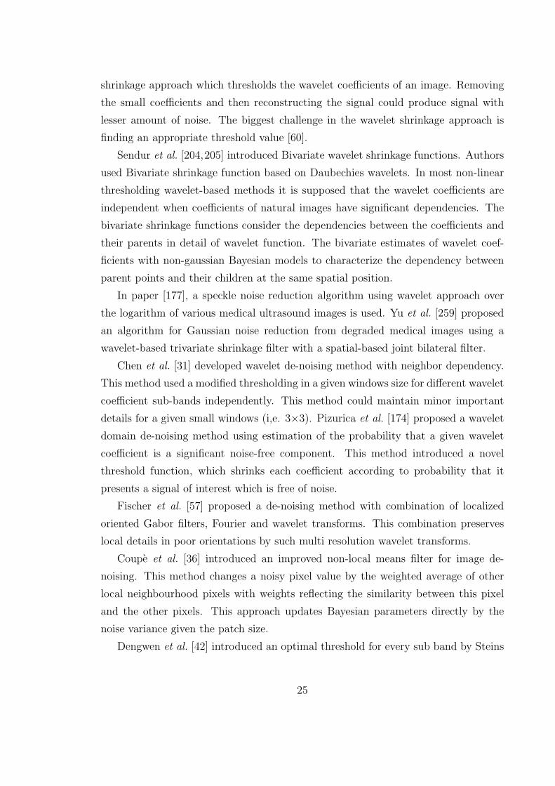
shrinkage approach which thresholds the wavelet coefficients of an image. Removing
the small coefficients and then reconstructing the signal could produce signal with
lesser amount of noise. The biggest challenge in the wavelet shrinkage approach is
finding an appropriate threshold value [60].
Sendur et al. [204,205] introduced Bivariate wavelet shrinkage functions. Authors
used Bivariate shrinkage function based on Daubechies wavelets. In most non-linear
thresholding wavelet-based methods it is supposed that the wavelet coefficients are
independent when coefficients of natural images have significant dependencies. The
bivariate shrinkage functions consider the dependencies between the coefficients and
their parents in detail of wavelet function. The bivariate estimates of wavelet coef-
ficients with non-gaussian Bayesian models to characterize the dependency between
parent points and their children at the same spatial position.
In paper [177], a speckle noise reduction algorithm using wavelet approach over
the logarithm of various medical ultrasound images is used. Yu et al. [259] proposed
an algorithm for Gaussian noise reduction from degraded medical images using a
wavelet-based trivariate shrinkage filter with a spatial-based joint bilateral filter.
Chen et al. [31] developed wavelet de-noising method with neighbor dependency.
This method used a modified thresholding in a given windows size for different wavelet
coefficient sub-bands independently. This method could maintain minor important
details for a given small windows (i,e. 3×3). Pizurica et al. [174] proposed a wavelet
domain de-noising method using estimation of the probability that a given wavelet
coefficient is a significant noise-free component. This method introduced a novel
threshold function, which shrinks each coefficient according to probability that it
presents a signal of interest which is free of noise.
Fischer et al. [57] proposed a de-noising method with combination of localized
oriented Gabor filters, Fourier and wavelet transforms. This combination preserves
local details in poor orientations by such multi resolution wavelet transforms.
Coupe et al. [36] introduced an improved non-local means filter for image de-
noising. This method changes a noisy pixel value by the weighted average of other
local neighbourhood pixels with weights reflecting the similarity between this pixel
and the other pixels. This approach updates Bayesian parameters directly by the
noise variance given the patch size.
Dengwen et al. [42] introduced an optimal threshold for every sub band by Steins
25
unbiased risk estimate (SURE) in a given neighboring window size. This method
profits from dual-tree complex wavelet transform (DT-CWT) as a shrinkage function
to alleviate redundant problem in typical wavelet.
In [265], Gaussian process regression (GPR), to detect edges with more detailed
information is addressed. In paper [17] computed tomography (CT) images have been
de-noised with combination of total variation (TV) and curve-let based methods. The
edged image is extracted from the left noise of TV algorithm by processing it through
curve-let transform.
Manjon et al. [136] first decomposes the signal into the local principal compo-
nents, then it shrinks the less relevant components, and lastly signal is reconstructed
as a free noise signal. The intuitive idea is that image can be represented as a linear
combination of a small number of basis images while the noise, being not sparse will
be spread over all available components. In a similar work image de-noising with
patch based PCA (local versus global) is also investigated. Deledalle et al. [27] intro-
duced three patch based de-noising algorithms which applied hard thresholding on
the coefficients. The algorithms differ by the methodology of learning the dictionary:
local PCA, hierarchical PCA and global PCA. Salmon et al. [199] takes advantage of
over-complete dictionaries combined with sparse learning techniques. This method
adapts a generalization of the PCA for de-noising degraded images by Poisson noise.
In terms of blood cell detection, in work [44] median filter is used to de-noise
blood microscopic images. Other work [135] proposed de-noising and blood image
enhancement by inter-scale orthogonal wavelet based threshold which is based on
stains unbiased risk estimator (SURE) approach.
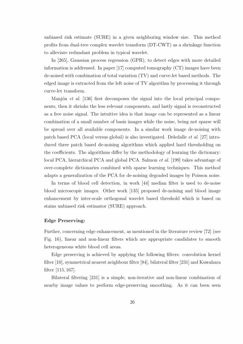
Edge Preserving:
Further, concerning edge enhancement, as mentioned in the literature review [72] (see
Fig. 16), linear and non-linear filters which are appropriate candidates to smooth
heterogeneous white blood cell areas.
Edge preserving is achieved by applying the following filters: convolution kernel
filter [10], symmetrical nearest neighbour filter [84], bilateral filter [231] and Kuwahara
filter [115,167].
Bilateral filtering [231] is a simple, non-iterative and non-linear combination of
nearby image values to perform edge-preserving smoothing. As it can been seen
26
from Bilateral filtering, two points are closeby pixels in which they are neighbours
in a spatial location, or they are close to one another in intensity values. This filter
considers similarity in geometric and photometric locality. This filter replaces the
value at x location with an average of similar pixel values. As a consequence, when
the bilateral filter is applied of the boundary, the bright pixel is replaced at the center
by an average of the bright pixels in its adjacent and nearby region, and it ignores
the dark pixels. It also reversely centred on a dark pixel then the bright pixels are
ignored instead. Finally, with using these steps image edges are preserved in some
extent. Symmetrical nearest neighbour (SNN) is based on distance measurement.
This filter compares symmetric 4-connected surrounded pixels in four directions (N-
S, W-E, NW-SE and NE-SW) with the center pixel and it only considers the pixel
from each paired set which is the closest to the center pixel value.
3.2 Research & Experimental Results
The prepared database (140 samples of five types) includes images of different con-
ditions for a sample referring to fig. 10. When images of blood smear have been
capturing, they are saved in JPEG (less computational requirements)format with 512
× 512 resolution. The calculation (see sub-section 3.2.1) shows that using the G
(green) channel is the best choice for converting the current blood smear images to
gray scale. Furthermore, the study examines the efficiency of Bayesian non local mean
de-noising technique in order to enhance cytological input images. After extensive
experimenting, the Kuwahara filter as a non-linear smoothing filter is chosen in this
study to smooth and preserve the white blood cell edges.
3.2.1 Colour Scale Channel
Computational outcomes have shown the adequate discrimination is achieved using
the ”Green” color channel [72]. It is obvious that Y channel is also an appropri-
ate alternative in case (see Table 4). Green encoding is better at maintaining high
frequency feature information [72].
Experiments on a set of 10 sample (different image characteristic (see Table 13)
blood smear images show that the green channel has a wider range of gray-level
values in the intensity histogram than the red and blue channels and thus keeps more
27
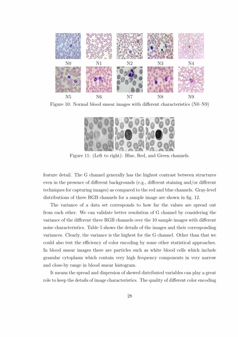
N0 N1 N2 N3 N4
N5 N6 N7 N8 N9
Figure 10: Normal blood smear images with different characteristics (N0–N9)
Figure 11: (Left to right): Blue, Red, and Green channels.
feature detail. The G channel generally has the highest contrast between structures
even in the presence of different backgrounds (e.g., different staining and/or different
techniques for capturing images) as compared to the red and blue channels. Gray-level
distributions of three RGB channels for a sample image are shown in fig. 12.
The variance of a data set corresponds to how far the values are spread out
from each other. We can validate better resolution of G channel by considering the
variance of the different three RGB channels over the 10 sample images with different
noise characteristics. Table 5 shows the details of the images and their corresponding
variances. Clearly, the variance is the highest for the G channel. Other than that we
could also test the efficiency of color encoding by some other statistical approaches.
In blood smear images there are particles such as white blood cells which include
granular cytoplasm which contain very high frequency components in very narrow
and close-by range in blood smear histogram.
It means the spread and dispersion of skewed distributed variables can play a great
role to keep the details of image characteristics. The quality of different color encoding
28
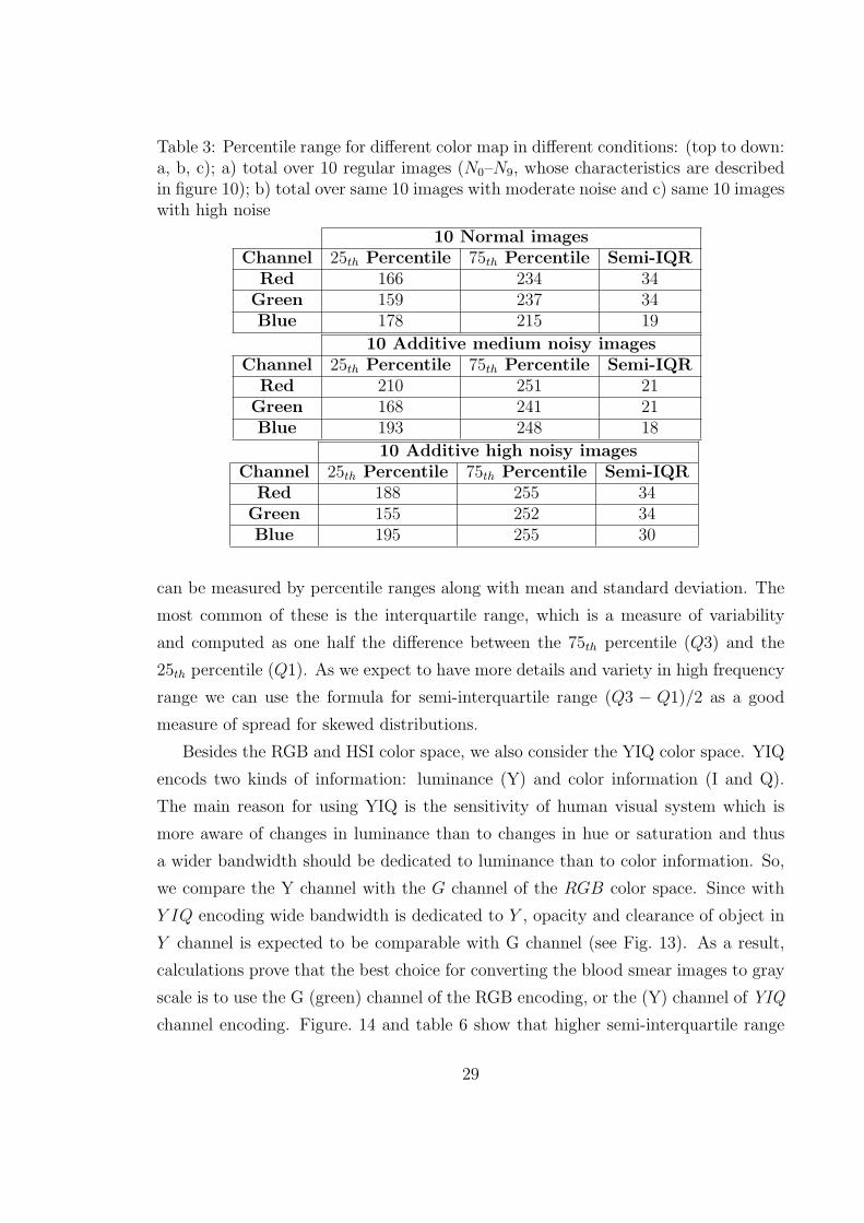
Table 3: Percentile range for different color map in different conditions: (top to down:a, b, c); a) total over 10 regular images (N0–N9, whose characteristics are describedin figure 10); b) total over same 10 images with moderate noise and c) same 10 imageswith high noise
10 Normal imagesChannel 25th Percentile 75th Percentile Semi-IQR
Red 166 234 34Green 159 237 34Blue 178 215 19
10 Additive medium noisy imagesChannel 25th Percentile 75th Percentile Semi-IQR
Red 210 251 21Green 168 241 21Blue 193 248 18
10 Additive high noisy imagesChannel 25th Percentile 75th Percentile Semi-IQR
Red 188 255 34Green 155 252 34Blue 195 255 30
can be measured by percentile ranges along with mean and standard deviation. The
most common of these is the interquartile range, which is a measure of variability
and computed as one half the difference between the 75th percentile (Q3) and the
25th percentile (Q1). As we expect to have more details and variety in high frequency
range we can use the formula for semi-interquartile range (Q3 − Q1)/2 as a good
measure of spread for skewed distributions.
Besides the RGB and HSI color space, we also consider the YIQ color space. YIQ
encods two kinds of information: luminance (Y) and color information (I and Q).
The main reason for using YIQ is the sensitivity of human visual system which is
more aware of changes in luminance than to changes in hue or saturation and thus
a wider bandwidth should be dedicated to luminance than to color information. So,
we compare the Y channel with the G channel of the RGB color space. Since with
Y IQ encoding wide bandwidth is dedicated to Y , opacity and clearance of object in
Y channel is expected to be comparable with G channel (see Fig. 13). As a result,
calculations prove that the best choice for converting the blood smear images to gray
scale is to use the G (green) channel of the RGB encoding, or the (Y) channel of YIQ
channel encoding. Figure. 14 and table 6 show that higher semi-interquartile range
29
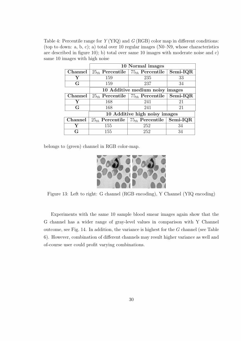
Table 4: Percentile range for Y (YIQ) and G (RGB) color map in different conditions:(top to down: a, b, c); a) total over 10 regular images (N0–N9, whose characteristicsare described in figure 10); b) total over same 10 images with moderate noise and c)same 10 images with high noise
10 Normal imagesChannel 25th Percentile 75th Percentile Semi-IQR
Y 159 235 33G 159 237 34
10 Additive medium noisy imagesChannel 25th Percentile 75th Percentile Semi-IQR
Y 168 241 21G 168 241 21
10 Additive high noisy imagesChannel 25th Percentile 75th Percentile Semi-IQR
Y 155 252 34G 155 252 34
belongs to (green) channel in RGB color-map.
Figure 13: Left to right: G channel (RGB encoding), Y Channel (YIQ encoding)
Experiments with the same 10 sample blood smear images again show that the
G channel has a wider range of gray-level values in comparison with Y Channel
outcome, see Fig. 14. In addition, the variance is highest for the G channel (see Table
6). However, combination of different channels may result higher variance as well and
of-course user could profit varying combinations.
30
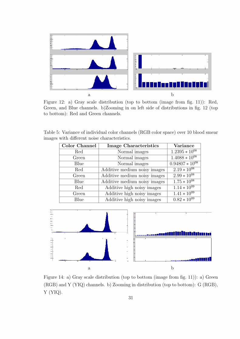
a b
Figure 12: a) Gray scale distribution (top to bottom (image from fig. 11)): Red,Green, and Blue channels. b)Zooming in on left side of distributions in fig. 12 (topto bottom): Red and Green channels.
Table 5: Variance of individual color channels (RGB color space) over 10 blood smearimages with different noise characteristics.
Color Channel Image Characteristics VarianceRed Normal images 1.2395 ∗ 1008Green Normal images 1.4088 ∗ 1008Blue Normal images 0.94807 ∗ 1008Red Additive medium noisy images 2.19 ∗ 1008Green Additive medium noisy images 2.99 ∗ 1008Blue Additive medium noisy images 1.75 ∗ 1008Red Additive high noisy images 1.14 ∗ 1009Green Additive high noisy images 1.41 ∗ 1009Blue Additive high noisy images 0.82 ∗ 1009
a b
Figure 14: a) Gray scale distribution (top to bottom (image from fig. 11)): a) Green
(RGB) and Y (YIQ) channels. b) Zooming in distribution (top to bottom): G (RGB),
Y (YIQ).31
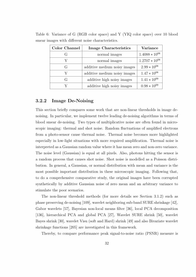
Table 6: Variance of G (RGB color space) and Y (YIQ color space) over 10 blood
smear images with different noise characteristics.
Color Channel Image Characteristics Variance
G normal images 1.4088 ∗ 1008
Y normal images 1.2707 ∗ 1008
G additive medium noisy images 2.99 ∗ 1008
Y additive medium noisy images 1.47 ∗ 1008
G additive high noisy images 1.41 ∗ 1009
Y additive high noisy images 0.98 ∗ 1009
3.2.2 Image De-Noising
This section briefly compares some work that are non-linear thresholds in image de-
noising. In particular, we implement twelve leading de-noising algorithms in terms of
blood smear de-noising. Two types of multiplicative noise are often found in micro-
scopic imaging: thermal and shot noise. Random fluctuations of amplified electrons
from a photo-sensor cause thermal noise. Thermal noise becomes more highlighted
especially in low-light situations with more required amplification. Thermal noise is
interpreted as a Gaussian random value where it has mean zero and non-zero variance.
The noise level (Gaussian) is equal at all pixels. Also, photons hitting the sensor is
a random process that causes shot noise. Shot noise is modelled as a Poisson distri-
bution. In general, a Gaussian, or normal distribution with mean and variance is the
most possible important distribution in these microscopic imaging. Following that,
to do a comprehensive comparative study, the original images have been corrupted
synthetically by additive Gaussian noise of zero mean and an arbitrary variance to
stimulate the poor scenarios.
The non-linear threshold methods (for more details see Section 3.1.2) such as
phase preserving de-noising [109], wavelet neighboring sub-band SURE shrinkage [42],
Gabor wavelets [57], Bayesian non-local means filter [36], local PCA decomposition
[136], hierarchical PCA and global PCA [27], Wavelet SURE shrink [50], wavelet
Bayes shrink [30], wavelet Visu (soft and Hard) shrink [49] and also Bivariate wavelet
shrinkage functions [205] are investigated in this framework.
Thereby, to compare performance peak signal-to-noise ratio (PSNR) measure is
32
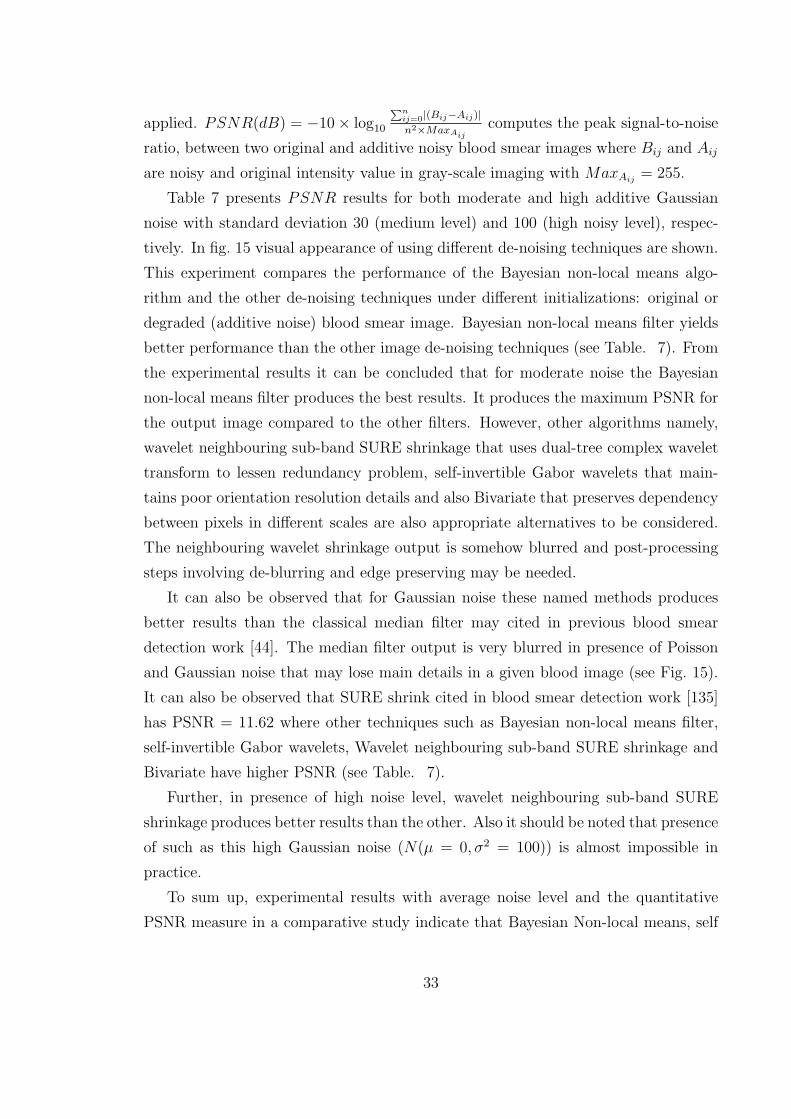
applied. PSNR(dB) = −10× log10
∑nij=0|(Bij−Aij)|n2×MaxAij
computes the peak signal-to-noise
ratio, between two original and additive noisy blood smear images where Bij and Aij
are noisy and original intensity value in gray-scale imaging with MaxAij = 255.
Table 7 presents PSNR results for both moderate and high additive Gaussian
noise with standard deviation 30 (medium level) and 100 (high noisy level), respec-
tively. In fig. 15 visual appearance of using different de-noising techniques are shown.
This experiment compares the performance of the Bayesian non-local means algo-
rithm and the other de-noising techniques under different initializations: original or
degraded (additive noise) blood smear image. Bayesian non-local means filter yields
better performance than the other image de-noising techniques (see Table. 7). From
the experimental results it can be concluded that for moderate noise the Bayesian
non-local means filter produces the best results. It produces the maximum PSNR for
the output image compared to the other filters. However, other algorithms namely,
wavelet neighbouring sub-band SURE shrinkage that uses dual-tree complex wavelet
transform to lessen redundancy problem, self-invertible Gabor wavelets that main-
tains poor orientation resolution details and also Bivariate that preserves dependency
between pixels in different scales are also appropriate alternatives to be considered.
The neighbouring wavelet shrinkage output is somehow blurred and post-processing
steps involving de-blurring and edge preserving may be needed.
It can also be observed that for Gaussian noise these named methods produces
better results than the classical median filter may cited in previous blood smear
detection work [44]. The median filter output is very blurred in presence of Poisson
and Gaussian noise that may lose main details in a given blood image (see Fig. 15).
It can also be observed that SURE shrink cited in blood smear detection work [135]
has PSNR = 11.62 where other techniques such as Bayesian non-local means filter,
self-invertible Gabor wavelets, Wavelet neighbouring sub-band SURE shrinkage and
Bivariate have higher PSNR (see Table. 7).
Further, in presence of high noise level, wavelet neighbouring sub-band SURE
shrinkage produces better results than the other. Also it should be noted that presence
of such as this high Gaussian noise (N(µ = 0, σ2 = 100)) is almost impossible in
practice.
To sum up, experimental results with average noise level and the quantitative
PSNR measure in a comparative study indicate that Bayesian Non-local means, self
33
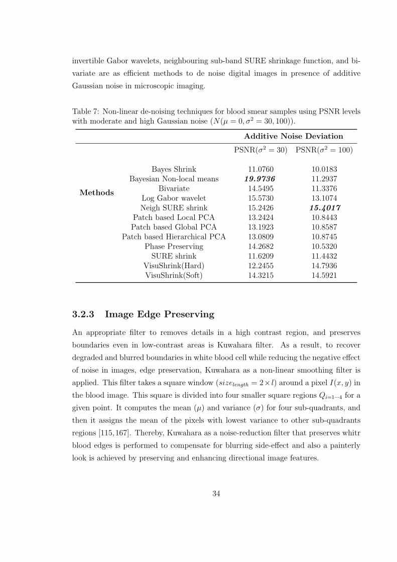
invertible Gabor wavelets, neighbouring sub-band SURE shrinkage function, and bi-
variate are as efficient methods to de noise digital images in presence of additive
Gaussian noise in microscopic imaging.
Table 7: Non-linear de-noising techniques for blood smear samples using PSNR levelswith moderate and high Gaussian noise (N(µ = 0, σ2 = 30, 100)).
Additive Noise Deviation
PSNR(σ2 = 30) PSNR(σ2 = 100)
Methods
Bayes Shrink 11.0760 10.0183Bayesian Non-local means 19.9736 11.2937
Bivariate 14.5495 11.3376Log Gabor wavelet 15.5730 13.1074Neigh SURE shrink 15.2426 15.4017
Patch based Local PCA 13.2424 10.8443Patch based Global PCA 13.1923 10.8587
Patch based Hierarchical PCA 13.0809 10.8745Phase Preserving 14.2682 10.5320SURE shrink 11.6209 11.4432
VisuShrink(Hard) 12.2455 14.7936VisuShrink(Soft) 14.3215 14.5921
3.2.3 Image Edge Preserving
An appropriate filter to removes details in a high contrast region, and preserves
boundaries even in low-contrast areas is Kuwahara filter. As a result, to recover
degraded and blurred boundaries in white blood cell while reducing the negative effect
of noise in images, edge preservation, Kuwahara as a non-linear smoothing filter is
applied. This filter takes a square window (sizelength = 2× l) around a pixel I(x, y) in
the blood image. This square is divided into four smaller square regions Qi=1···4 for a
given point. It computes the mean (µ) and variance (σ) for four sub-quadrants, and
then it assigns the mean of the pixels with lowest variance to other sub-quadrants
regions [115,167]. Thereby, Kuwahara as a noise-reduction filter that preserves whitr
blood edges is performed to compensate for blurring side-effect and also a painterly
look is achieved by preserving and enhancing directional image features.
34
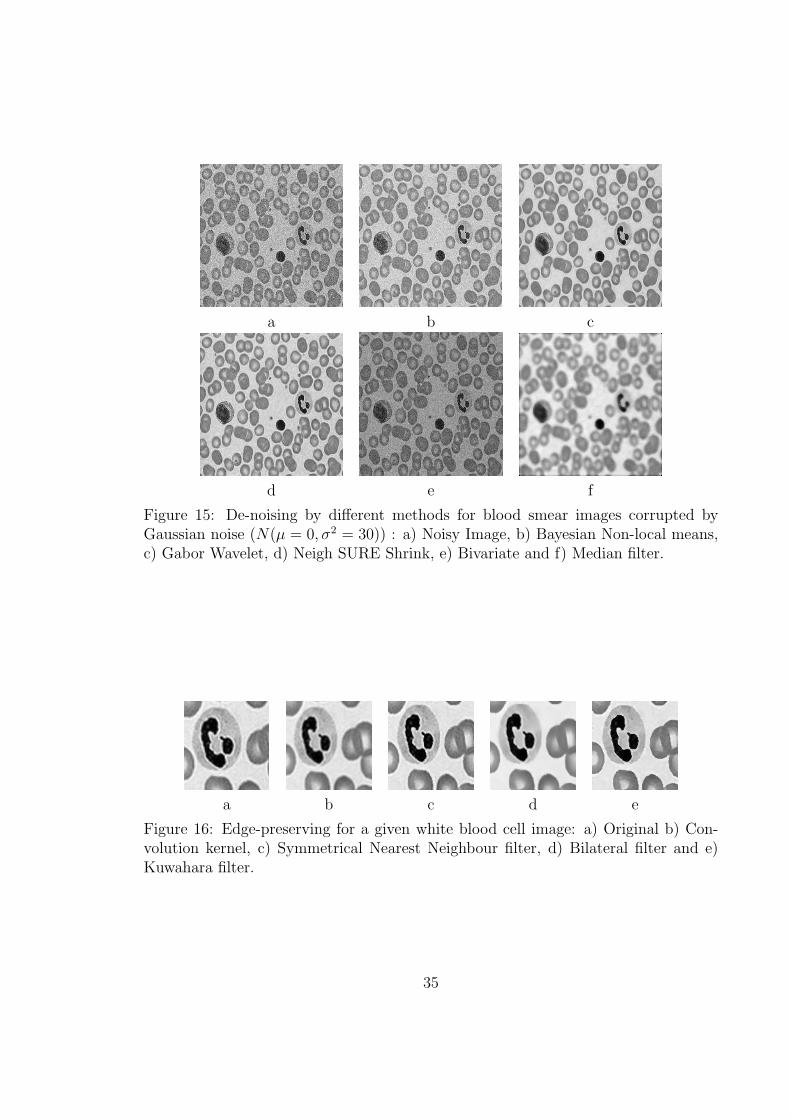
a b c
d e f
Figure 15: De-noising by different methods for blood smear images corrupted byGaussian noise (N(µ = 0, σ2 = 30)) : a) Noisy Image, b) Bayesian Non-local means,c) Gabor Wavelet, d) Neigh SURE Shrink, e) Bivariate and f) Median filter.
a b c d e
Figure 16: Edge-preserving for a given white blood cell image: a) Original b) Con-volution kernel, c) Symmetrical Nearest Neighbour filter, d) Bilateral filter and e)Kuwahara filter.
35
3.2.4 Pre-Processing Settings
This section gives a brief overview of initial settings with regard to image enhance-
ment and pre processing steps (see Figs. 5,6). This section briefly explains how each
parameter is set. There are many challenging problems in setting these parameters in
an ideal efficient way and some changes are inevitable to apply for different dataset.
However, the most parameters could be kept unchangeable.
Colormap Selection
This study uses JPEG format (see Section 3.1). Following that, to choose a proper
gray scale channel statistical approaches such as variance and semi interquartile are
addressed. These two measures determine whether local details are enough kept (see
Tables 4, 5). There is no parameter that should be set manually.
Denoising Selection
This framework uses Bayesian non-local mean [36], Gabor wavelet [57], Bivariate [205]
and neighbouring SURE shrink function [42] (see Table 7). These candidates require
initialization and setting before going further to use them. These settings are in
table 8.
Image Abstraction
As for white blood cell detection, edge preserving and image abstraction is addressed
using Kuwahara filter (see Fig. 16). Kuwahara filter is by a sliding windows with where
its parameters namely, mean and standard deviation are automatically calculated in
four sub-regions in a defined sliding windows. This size should be enough small to
cover all details. To sum up, only windows size is manually set (15× 15). Of course,
it is obvious smaller windows just only increase running time and there is no more
burden than increasing computational time.
36
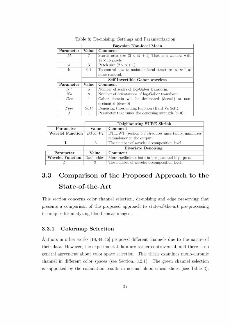
Table 8: De-noising: Settings and Parametrization
Bayesian Non-local MeanParameter Value Comment
M 7 Search area size (2 × M + 1) That is a window with15× 15 pixels.
α 3 Patch size (2× α + 1).h 0.1 To control how to maintain local structures as well as
noise removal.
Self Invertible Gabor waveletsParameter Value Comment
Nf 5 Number of scales of log-Gabor transform.No 8 Number of orientations of log-Gabor transform.Dec 1 Gabor domain will be decimated (dec=1) or non-
decimated (dec=0)Type Soft Denoising thresholding function (Hard Vs Soft).f 1 Parameter that tunes the denoising strength (> 0).
Neighbouring SURE ShrinkParameter Value Comment
Wavelet Function DT CWT DT CWT (section 5.3.3)reduces uncertainty, minimizesredundancy in the output.
L 3 The number of wavelet decomposition level.
Bivariate DenoisingParameter Value Comment
Wavelet Function Daubechies More coefficients both in low pass and high pass.L 3 The number of wavelet decomposition level.
3.3 Comparison of the Proposed Approach to the
State-of-the-Art
This section concerns color channel selection, de-noising and edge preserving that
presents a comparison of the proposed approach to state-of-the-art pre-processing
techniques for analyzing blood smear images .
3.3.1 Colormap Selection
Authors in other works [18, 44, 46] proposed different channels due to the nature of
their data. However, the experimental data are rather controversial, and there is no
general agreement about color space selection. This thesis examines mono-chromic
channel in different color spaces (see Section. 3.2.1). The green channel selection
is supported by the calculation results in normal blood smear slides (see Table 3).
37
The green channel is better at maintaining high frequency feature information and
contrasts in gray scale intensity that are more easily distinguished in the G channel.
The high frequency information is essential to preserve white blood cells structure in
particular (see Fig. 11). However, combination of different channels with weighting
of individual channels to achieve a desired appearance is not addressed in this thesis
and will be in the future.
3.3.2 Denoising Selection
As for blood cell detection, there is a considerable volume of published studies de-
scribing the role of median filter in blood samples de-noising. In work [18, 44, 46]
and also in malaria research [224, 225, 226] median filter is used to de-noise blood
microscopic images.
Median filter is an appropriate technique to remove salt-and-pepper noise where
pixel looks much different from its neighbours. Median filtering often fails to pro-
vide agreeable smoothing of non-impulsive noise where the underlying object has
edges [25,152] and its result could be unpredictable for different dataset. Perhaps the
most serious disadvantage of this median method is that there is no way to address
correlation and dependency between pixels and then it adversely reduces the visibility
of certain features within the image. Moreover, the median filtering approach is not
efficient for the images with large amounts of Gaussian noise or speckle noise [152].
Median filter depends on sliding windows size and once intensity values are nearly
small compared to the size of the pre-determined neighbourhood, it will adversely
change the median value and then eventually the median filter cannot sort out image
detail from undesirable noise. As a result, median filter is not an appropriate can-
didate for blood smear images with these nature of noise that may address in blood
smear imaging (see Section. 3.2.2).
Other work in 2011 [135] explored wavelet de-noising by inter-scale orthogonal
wavelet which is based on stains unbiased risk estimator (SURE) approach. In this
method, as it can be seen from literature review, it is assumed that the wavelet
coefficients are independent and there is no connection in different wavelet scales.
However, independence assumption may not be satisfied for natural images and blood
smear samples.
In conclusion, as it can be seen from results, Bayesian non local mean, optimal
38
threshold using SURE shrinkage function with dual tree complex wavelet and neigh-
bouring window, self-invertible 2D Log-Gabor wavelets and Bivariate filter bring ben-
efit in blood smear de-noising (see Table 7) in presence of different Gaussian noise
level.
3.3.3 Image Abstraction
Previous studies of white blood cell segmentation have not dealt with this possible
adverse condition in blood smear slides where boundaries are messy, granular and in
low faded conditions. Experimental results show that Kuwahara and Bilateral filters
are proper candidates to build better outcome close to the expected boundaries. In
general, Kuwahara is superior to Bilateral in this application (see Fig. 16). Kuwahara
filter brings two benefits together. It expands homogeneous region in cytoplasm to
its heterogeneous neighbours using a sliding windows. This approach thus removes
unwanted color details in cytoplasm that they are not needed in this low resolution
images. Secondly, as mentioned before white blood cells do not have determined edges.
This filter makes a sharp pixels next to non-obvious edges. As a result, existing sharp
pixels close to possible edge and also removing unnecessary details bring benefits for
next steps in white blood cell segmentation (see Section. 4.4.2) and also in feature
extraction (see Section. 5.5).
3.4 Pre-Processing Findings and Contributions
One of the contributions is the pre-processing, for enhancing the appearance of the
shape. It includes color channel selection, de-noising and edge preserving that are
explained in details as follow. Colour space selection would be automated using
distribution behaviour calculations to keep local and global details. This De-noising
algorithm is a significant development as the most commonly used approaches, i.e.
Median filter, can not be used when the nature of noise is either Gaussian or unknown.
And also the results of the edge preserving are found to be promising when the white
blood cells having degraded internal structure and almost invisible boundaries.
39
3.4.1 Colormap Selection
This work proposed a statistical calculation for analyzing the color map selection in
presence of different possible color spaces (see Section. 3.1.1). The method is based
on a variance and semi interquartile that enables us to test how low and high fre-
quency information can be accumulated. These details are very critical in presenting
white blood cells where boundaries and their internal structure are very fragile and of
course inappropriate selection leads inevitable problems in next framework step. For
example, blue channel in current dataset is unable to maintain intensity details sep-
arately (see Fig. 11). Authors in other works proposed different channels due to the
nature of their data. Comparative study and discussion is addressed in section 3.4.1.
However, combination of different channels with weighting of individual channels to
achieve desired appearance is left for future study.
3.4.2 Denoising
This work has empirically tested different de-noising mechanisms for a given intensity
blood image. As for blood cell detection, there is a considerable volume of published
studies describing the role of median filter in blood samples de-noising. In addition,
few work used SURE wavelet shrinkage as well. Discussion will be found in sec-
tion 3.3.2. In conclusion, as it can be seen from presented results that Bayesian non
local mean, optimal threshold using SURE shrinkage function with dual tree complex
wavelet and neighboring window, self-invertible 2D Log-Gabor wavelets and Bivari-
ate filter bring benefit in blood smear de-noising (see Table 7) in presence of different
Gaussian noise level produce the best results.
3.4.3 Image Abstraction
Third, in terms of blood cell detection, white blood cell is with low contrast boundaries
and weak edges. The Kuwahara edge preserving is highly suited to enhance poor
visibility conditions (see Fig. 32). Experimental results and discussion is found in
section 3.3.3 and figure 16. As a result, existing sharp pixels close to possible edge
and also removing unnecessary details bring benefits for next steps in white blood
cell segmentation (see Section 4.4.2) and also in feature extraction (see Section 5.5).
40
Chapter 4
Blood Binarization & Cell
Separation
After de-noising and artistic edge enhancement, binarization is the third step which
allows to extract some features, having sub images and get ready to apply techniques
for different purpose over the images. This work proposes a modified binarization
method that reduces limitations and drawbacks of each local and global thresholding.
Binarization and some post-processing to enhance the quality of binary image is
followed by cell size estimation which helps to differentiate various types of particles in
the blood smear image. The size estimation approach is chosen in this step because it
identifies several advantages of the case study. Normal red blood cells in particular are
found with an average size distribution in healthy people. Moreover, cell separation
into two sub-groups including white blood cells and red blood cells is followed also
on using size parameter.
Further, a key step in many experimental blood smear analysis involves counting
of red blood cells and white blood cell differential (see Section 1.2.1). A simple
counting of cells brings different benefits for health system and provides a great help
in detecting problems at early stages.
4.1 Problem Statement
After pre-processing (denoising and edge enhancement), binarization is the third step
which allows to extract WBCs and RBCs sub-images, compute the RBCs size and
41
count them. The aim of this section is to determine which algorithm is the most
reliable and robust for binarization of medical images, specifically used in blood cells.
Generally, binarization can be applied with either global or local thresholding
where both have intrinsic problems. For the global approach, a constant intensity
threshold value T (between 0 and 255) is chosen. If the intensity value of any pixel
(in the grey scale) of an input image is greater than T, then pixel is set to white
otherwise it is set to black. A global threshold (T) which maximizes the variance
between the means of the histogram classes on each side of the threshold is selected.
On the other side, a local thresholding technique depends on the window size moving
over the image that it separates background with local statistics measures.
Global binarization argument relies heavily on quantitative analysis of one unique
threshold value in which most local approaches use adaptive local values. Uniform
contrast distribution in most cases leads to global thresholding unlike in presence of
degraded images, complex scene images, variation in contrast and illumination. In
these aforementioned conditions, global thresholding may fail to resolve the contra-
diction between background and foreground.
Different algorithms have already introduced to improve both local and global
thresholding of digital images. In general, no identical binarization algorithm is supe-
rior to others. However, some methods are better than others for specific applications.
The goal in this study is to obtain a robust binarization method to allow for further
blood image content clarification. Binarization is the last step before computing cell
sizes and their enumeration.
Further, a normal blood cell is one of two major particles: a RBC with a normal
probability distribution function (PDF) with average size around 6.0-8.5 µm or a
WBC with average size around 7-18 µm which includes a nucleus and cytoplasm.
Mature WBC is about equal normal RBC size (i.e, Basophil) up to 3 times bigger
than normal and mature RBCs (see Section. 1.2).
As mentioned in medical background (see Section 1.2.1), size is a key parameter
to identify the blood sample health. Also, as mentioned earlier (see Section 1.2.1),
the red cell distribution width (RDW) is an expression of the red blood cell (RBC)
size distribution in complete blood count (CBC) report.
We use size characteristics as an effective factor to distinguish between the two
main types of cells that are RBCs and WBCs. Red blood cells size estimation is
42
an essential task at various stages of blood slide processing to go further in cell
segmentation. We aim to have two sub-images containing individual white blood
cells and red blood cells are separated in order to count cells in CBC medical test.
The aim of segmentation is to isolate each individual blood cells, especially when they
are close and overlapping in the viewing of the microscope.
It locates and recognizes the cell contours to distinguish amongst them. An inac-
curate segmentation leads to ulterior quantification and parameter measurement. The
goal of our CBC segmentation and counting research is to find methods partitioning
the digital blood smear image into non-intersecting regions; RBCs and WBCs.
Finally, thus far, after cell separation we have two individual sub-images for RBCs
and WBCs and have localized the WBCs. A complete medical CBC reports number
of cells to properly understand a patients health. In particular, the distribution of
the different subtypes and proportional rate in a blood sample is CBC interest.
4.2 Literature Review
To the author’s best knowledge, there are no comparative evaluations of the efficiency
of binarization algorithms at binarizing medical blood smear images.
4.2.1 Global Thresholding
A considerable amount of literature has been published on global binarization. Ridler
and Calvard (1978) [190] developed a binarization algorithm while retaining the ap-
propriate possible illumination of the image. In 1979 Otsu [164] classified foreground
and background with a global threshold. The optimum threshold in Otsu method is
selected automatically by using the probability terms whereas it maximizes variance
between-class and minimizes variance within-class. Other than Otsu algorithm, there
is a large and growing body of global thresholding schemes have been proposed such
as algorithm of Kapur et al. [97]; Fan et al. [55]; Portes de Albuquerque et al. [40];
and also Xiao et al. [251]. It should be noted that among all these global binarization
studies, Otsu [164] is frequently cited.
43
4.2.2 Local Thresholding
Locally adaptive binarization methods compute a threshold for each pixel in the im-
age on the basis of information appeared in a neighbourhood of a given pixel. During
the two last decades, a lot of information has become available on local threshold-
ing. The first discussion and analyse of local thresholding backs to 1972 with Chow
and Kaneko algorithm [32]. In that method, original image is divided into a set
of regions. Intensity histograms are computed for all sub-divided sections and then
thresholding value will be selected for these histograms. All predefined local thresh-
olding values are interpolated twice times first region-wise and then point-wise to
obtain a threshold for the original image. Numerous studies have been attempted to
reach better performance in different applications. They are more promising locally
adaptive binarization methods that we could mention in the literature.
Bernsen [16] in 1986, introduced a method which is based on a given contrast
threshold in a sliding window. The pixel is set at the mean of the minimum and
maximum grey values in the sliding window if local contrast is above the predefined
contrast. Otherwise, it is set to background. The contrast value is arbitrary where
default value is recommended to be set at 15.
Niblack [155] in 1990, introduced a binarization algorithm using two values that
are mean and standard variation in a sliding window. The size of the window must
be large enough to suppress the noise amount in the image as well as be also small
enough to maintain local details. In practice, a window size of 15-by-15 could be an
appropriate selection. This method can work roughly without user intervention as it
requires only a coefficient value that helps to separate and adjust the percentage of
pixels that belong to foreground (especially in the boundaries). The default value is
0.2 for bright objects and -0.2 for dark objects. In Current application as cells (see
Fig. 10) are almost darker than background we could use k = −0.2.
Sauvola [201] in 2000, also introduced a local thresholding method using means
and standard variation in a sliding window. Sauvola is almost considered as a vari-
ation of Niblack’s method. However, the formulation has a little difference and it
has two parameters to be adjusted. Parameter (k) that default value is 0.5 and (r)
that usually is 128. These two value are very questionable and the existing default
fail to resolve the contradiction between foreground and background with different
conditions. Overall, these setting are almost arbitrary and could be changed with
44
different dataset and user interference is addressed to some extent.
Feng et al. in 2004, introduced a local thresholding method [56] with using many
parameter settings. Feng method is an appropriate candidate to maintain informa-
tion from a given image, especially for poor quality, non-uniform illumination, low
contrast samples. This method can qualitatively outperform the other threshold-
ing methods. However, the Feng method contains many parameters. This method
used two sliding windows with different size to preserve the details. The thresh-
old value is calculated where α, γ, K1 and K2 are positive constants that they rely
on the nature of dataset. Padding parameter should be also set which are circular,
replicate and symmetric. Feng argument relies heavily on quantitative analysis of
image parametrization. This method requires calibration through different iterations
of testing and retuning. One of the limitations with this explanation is that it does
not explain how parameters could be set automatically to some extent. The optimum
window size and other parameters can be adjusted using different experimental results
and this system requires user surveillance. Hence, this method is not recommended
widely for an semi-automated system without user intervention.
Gatos et al. in 2006, [65] introduced a two-step approach to build a local threshold-
ing method. First Sauvola’s method is applied and then local threshold values based
on the estimated background are computed. This method could be an appropriate
option in presence of degraded and complex background. However, background esti-
mation can be addressed in different ways [64,142] and there is no superior identical
method that can be used for different backgrounds with varying conditions.
Bradley et al. in 2007, [22] introduced a local thresholding method that a given
pixel is considered as a foreground if its brightness value is lower than the average
brightness of the surrounding pixels in a given sliding window. The amount of differ-
ence is calibrated using a percentage value (T) and should be adjusted empirically.
This manual settings can be changed for different circumstance and dataset. However,
the advantage of this method is its low computational time and only on T param-
eter adjustment. Bradley method is two times faster than Sauvola’s method [201].
Local mean and variance are computed in Sauvolas method, while Bradleys method
calculates just local mean and variance can be calculated using expected value.
Su et al. [219] in 2010 proposed an edge-based local threshold method that it
computes image contrast. Their approach profits combination of canny as an edge
45
detector and Otsu to Binarize images. This method is good at removing heterogeneous
background noise but it may fails to detect the degraded, low resolution and close-by
objects.
Hedjam et al. [86] in 2011 used a prior information and the spatial relationship
on the image. This method used Gaussian distribution to model foreground and
background where as the first step, Sauvolas method is used to Binarize original
image. This method is based on known local prior information of the background
and foreground. However, there is an inconsistency with this argument.
Ntirogiannis et al. in 2014 proposed [157] proposed a combination of a global and
a local thresholding binarization method at connected component level to reach better
performance in presence of variety of degraded handwritten document images. The
method profits combination of Niblack and Otsu algorithm on normalized images.
This combination and discussion is very close to already our published paper in 2011
and 2012 [72,78].
4.2.3 Blood Smear Binarization
To date, the blood smear researches are more about on global thresholding methods
rather than local thresholding methods. Some papers on blood segmentation such
as [15], [242] and also one of frequently cited work [46] all tried global thresholding
method using the well known Otsu method. The existing global Otsu thresholding
value fails to resolve different conditions that exist in blood slide images. A serious
weakness with this argument, however, is that known but also it does not manage
binarization with nearby background and foreground intensity values range [78].
No research has been found concerning combination of global and local thresh-
olding in microscopic imagery systems. This research discusses the challenges and
strategies to manage binarization in presence of different unfavourable conditions in
a typical blood smear image.
4.2.4 RBC Size Estimation
There is a considerable volume of published studies describing the role of Granu-
lometry for size estimation in mathematical imaging and vision. Granulometry is a
known method to extract blood smear size characteristics. Automatic thresholding
46
using Granulometry and regional maxima in image pattern spectrum are addressed
in some blood studies such as [14,41,46,194,226]. Granulometry and its applications
will be explained in the section. 4.3.2.
4.2.5 RBCs & WBCs separation
A serious attempt to segment in order to count backs to Vincent et al. work with mor-
phological filter to reconstruct segmentation in image analysis in 1993 [239]. Svensson
et al. described a decomposition scheme by a fuzzy distance transform to separate ob-
jects into sub-parts [221]. Li et al. [125] introduced a framework to segment nuclei in
images where their framework is based on three steps including a gradient approach,
flow tracking and grouping, and finally local adaptive thresholding.
Hoover et al. [88] described an automated framework to locate blood vessels using
match filter and thresholding algorithms. Jelen et al. [94] addressed nuclei segmen-
tation on breast cancer malignancy classification with level set, fuzzy cmeans seg-
mentation. Quelhas et al. [176] introduced sliding band filter to locate cell nuclei
and cytoplasm with evaluation for two datasets of cell culture images. Sadeghian et
al. [198] introduced a frame work to segment white blood cells using image gradients,
edge detection algorithms. Dorini et al. [51] introduced nucleus and the cytoplasm
segmentation with self-dual multi-scale morphological toggle (SMMT) filter along
with scaled erosion and dilation morphological operations to improve the correctness
and performance of two known watershed transformation and level sets segmentation
approaches. In an important work Di Ruberto et al. [46] used classical area opening
(see Fig. 26) morphology technique to separate between WBCs and RBCs. Authors
claimed to isolate the white cells by a morphological erosion with a disk-shaped struc-
turing element whose size is achieved by the granulometric analysis (RBC size). This
approach has some drawbacks. It just neglected overlapping phenomena among cells.
It is not also efficient for all possible five WBCs types where Basophil (fig. 1) can be
possible found the RBC size. Some previous studies have focused on the implementa-
tion of active contours to extract blood cell boundaries in white blood cell study [80].
Blood vessel segmentation using active contours is also addressed in [43]. Active con-
tours [191] require initialization and additional regularizers and therefore, the active
contour using a level set adjustment in some cases is costly and also makes unwanted
extra spurious regions as fake boundaries.
47
4.2.6 RBC Counting
Watershed is frequently used for an automatic contour detection and cell segmenta-
tion [131, 240]. First idea of watershed comes from geography topographic concepts
where water divides lines of the domains of attraction of rain falling over the region
(Tobbogan method). An alternative approach is where landscape being immersed in
a water, with holes pierced in local minima that are called Basins. These two ap-
proaches [131] are interpreted as follow. Immersion starts from low altitude to high
altitude while Toboggan approach starts from high altitude to low altitude. Water-
shed in image processing isolates objects from the background into disjoint regions
(see Fig. 28).
4.3 Research & Experimental Results
4.3.1 Blood Binarization
To separate blood particles (foreground) from background the binarization step is ap-
plied. In this study , the foreground objects are RBCs and WBCs while the remaining
objects such as platelets, artefacts in peripheral blood smear and stained plasma are
declared as background.
In the blood smear images slides, because of different kinds of image acquisition,
illumination, staining and when the intensity variations between the cells and stained
plasma are low, and since there are frequently overlapping and very closely positioned
particles, finding a global value T (Thresholding) to separate the image into two ideal
regions of blood particles and background is not always simple and perhaps not even
possible (closely positioned pairs of particles will be merged into single particles,
regardless of any fine tuning of the value of T ). After pre-processing which are
denoising and edge enhancement; several binarization algorithms including Niblack
[102], Bernsen [16], Sauvola [201], Feng algorithm [56], Wolf & Jolion [247], Bradley
[22] and Otsu [164] to enable foreground background separation improvement of blood
smear microscopic images (see Fig. 17) can be candidates where in practice we have a
variety of intensities of grey in the blood smear images. This contribution is directed
toward a robust binarization method in blood smear digital diagnosis. In Niblack
[102], the local thresholding is based on T (x, y) = m(x, y)+ k ∗ s(x, y), where m(x, y)
48
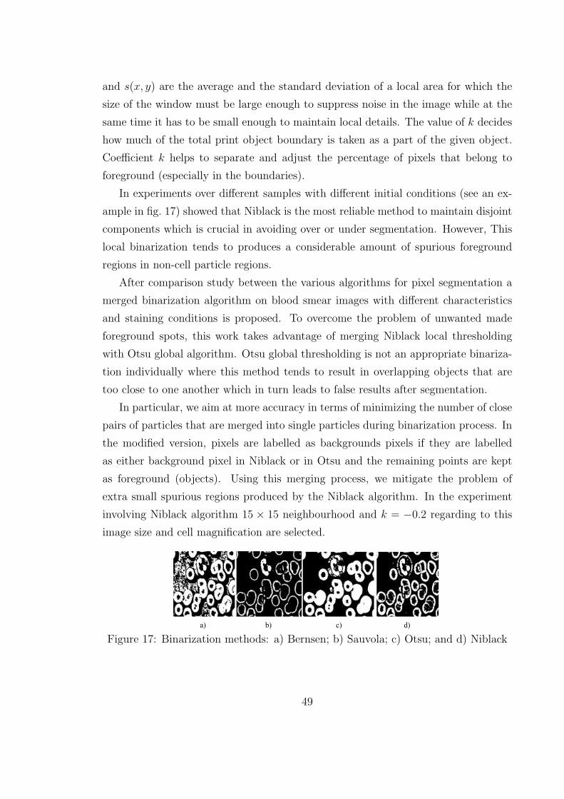
and s(x, y) are the average and the standard deviation of a local area for which the
size of the window must be large enough to suppress noise in the image while at the
same time it has to be small enough to maintain local details. The value of k decides
how much of the total print object boundary is taken as a part of the given object.
Coefficient k helps to separate and adjust the percentage of pixels that belong to
foreground (especially in the boundaries).
In experiments over different samples with different initial conditions (see an ex-
ample in fig. 17) showed that Niblack is the most reliable method to maintain disjoint
components which is crucial in avoiding over or under segmentation. However, This
local binarization tends to produces a considerable amount of spurious foreground
regions in non-cell particle regions.
After comparison study between the various algorithms for pixel segmentation a
merged binarization algorithm on blood smear images with different characteristics
and staining conditions is proposed. To overcome the problem of unwanted made
foreground spots, this work takes advantage of merging Niblack local thresholding
with Otsu global algorithm. Otsu global thresholding is not an appropriate binariza-
tion individually where this method tends to result in overlapping objects that are
too close to one another which in turn leads to false results after segmentation.
In particular, we aim at more accuracy in terms of minimizing the number of close
pairs of particles that are merged into single particles during binarization process. In
the modified version, pixels are labelled as backgrounds pixels if they are labelled
as either background pixel in Niblack or in Otsu and the remaining points are kept
as foreground (objects). Using this merging process, we mitigate the problem of
extra small spurious regions produced by the Niblack algorithm. In the experiment
involving Niblack algorithm 15 × 15 neighbourhood and k = −0.2 regarding to this
image size and cell magnification are selected.
a) b) c) d)
Figure 17: Binarization methods: a) Bernsen; b) Sauvola; c) Otsu; and d) Niblack
49
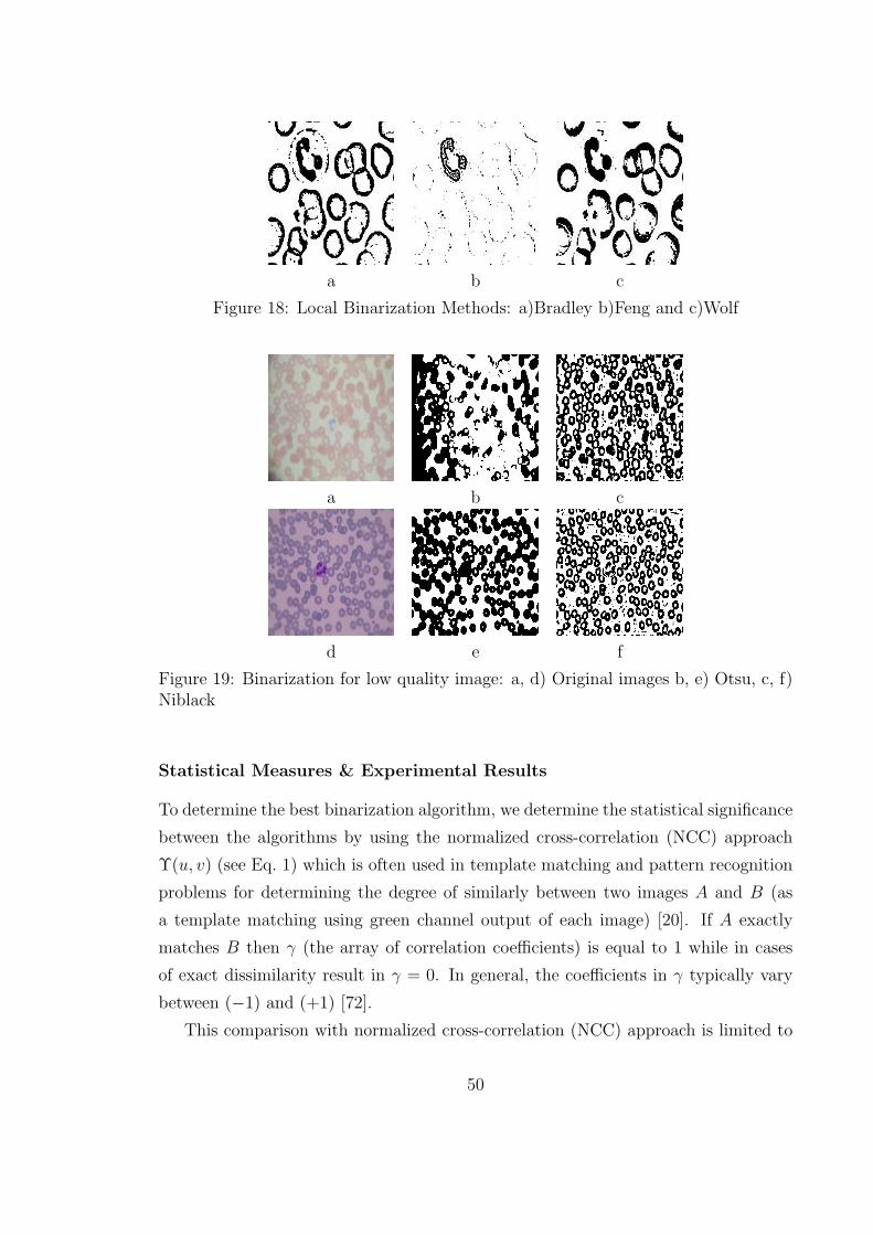
a b c
Figure 18: Local Binarization Methods: a)Bradley b)Feng and c)Wolf
a b c
d e f
Figure 19: Binarization for low quality image: a, d) Original images b, e) Otsu, c, f)Niblack
Statistical Measures & Experimental Results
To determine the best binarization algorithm, we determine the statistical significance
between the algorithms by using the normalized cross-correlation (NCC) approach
Υ(u, v) (see Eq. 1) which is often used in template matching and pattern recognition
problems for determining the degree of similarly between two images A and B (as
a template matching using green channel output of each image) [20]. If A exactly
matches B then γ (the array of correlation coefficients) is equal to 1 while in cases
of exact dissimilarity result in γ = 0. In general, the coefficients in γ typically vary
between (−1) and (+1) [72].
This comparison with normalized cross-correlation (NCC) approach is limited to
50
only four appropriate candidates (see Fig. 17) in this experiment. The experimen-
tal data in other cases are rather controversial, and there is no general agreement
about their usefulness (see discussion in section. 4.2.2). In some cases, like Feng algo-
rithm [56], many parameters adjustments are necessary, which, in turn, requires user
intervention for different conditions due to overload.
γ(υ, ν) =
∑x,y
[A(x, y)− Aυ,ν ][B(x− υ, y − ν)− B]
{∑x,y
[A(x, y)− Aυ,ν ]2∑x,y
[B(x− υ, y − ν)− B]2
}1/2(1)
The resulting coefficients in the matrix of normalized cross-correlation (NCC)
cannot all be needed and then the measurement of performance and efficiency are
subjected to a comparison using the average (expressed as the mean, median, and
mode), standard deviation and range to show how much variation or dispersion there
is between existing values.
In our experimentation to study the effect of noise on binarization results, we
degrade the objects (foreground) in samples by adding noise including Gaussian and
speckle noise to simulate worst cases that may appear in image capturing. Also to
simulate dirty slides or camera lens a 2, 3 pixel Gaussian blur to the samples is
applied.
The following tables present the results obtained from the preliminary analysis of
normalized cross-correlation (NCC). The result has been divided into three parts.
The first part (see Table 9) deals with all 10 sample blood images (see Fig. 10). Then
it goes for for separated white blood cell images (table 10). Finally, the last table
investigated the impact of binarization on red blood cells (table 11). In terms of
NCC value the largest means are generated by Otsu as a global thresholding and the
dispersion and variation is low which prove the acceptable degree of similarity between
image and its template. However, in WBC segmentation and discrimination between
WBCs and RBCs this approach may fail and also this algorithm merges disjoint close
by objects as it uses global thresholding over all slides and then local details are not
kept. WBCs nucleus and cytoplasm intensity vary from the intensity of dominant of
RBCs and as the number of RBCs is about 100 times more than WBCs then global
thresholding is influenced by RBCs rather than WBCs. Therefore, WBC boundary
and its components are degraded and damaged based on Otsu global thresholding in
51
spite of having higher template matching.
Next, this calculation has also been applied to separated regions composing of
a single WBC and few RBCs, with small gaps between these objects (see Fig. 17).
The NCC shows Niblack algorithm brings higher NCC performance. However, in
Niblack, because of using local thresholding, a minor background difference in in-
tensity value, makes spurious objects may results such as unwanted fake foreground
spots. As a result, after enough investigation the desired result is achieved with higher
NCC in a small windows (Niblack) including WBCs and few close by RBCs (better
segmentation in foreground) with along higher NCC value in global thresholding by
Otsu to avoid having spurious spots in background. Admittedly, merged these two
Niblack and Otsu develops a methodology for the selective binarization. The results
obtained from the preliminary analysis of NCC are shown in following tables (see Ta-
bles. 9,10,11). In the experiment involving Niblack algorithm 15×15 neighbourhood
and k = 0.1 regarding to this image size and cell magnification are selected. The
experimental results indicate that merged Niblack and Otsu is enough sufficient to
obtain foreground and background separation.
4.3.2 RBC Size Estimation
Granulometry [206] results size distribution in pattern spectrum diagram (output).
Granulometry algorithms involve sequences of openings (I ◦SE = (I⊖SE)⊕SE) or
closings ((I⊕−SE)⊖(−SE)) derived from the erosion and dilation of increasing size,
where I and SE are image and structure element. ⊖ and ⊕ also denote the erosion
and dilation, respectively. Granulometry is determined with ∀x ∈ I; x 7→ s+λs× x
where S is a homothetic center and λ is an expanding non - zero ratio. Granulome-
try is commonly interpreted to a maximum of morphological opening morphological
operation (or closings) with the homothetic transformation which is an increasing
affine transformation space of a simple convex structuring element (SE). Typically,
structuring element (SE) is a line segment, a circle, a square, or a hexagon.
Edge Fracture in Granulometry
In broadly speaking, Granulometry uses a series of morphological opening operations
to estimate a size distribution of particles in digital images. As a expected result,
in an ideal output, we should have only one peak for a single complete circle, but
52
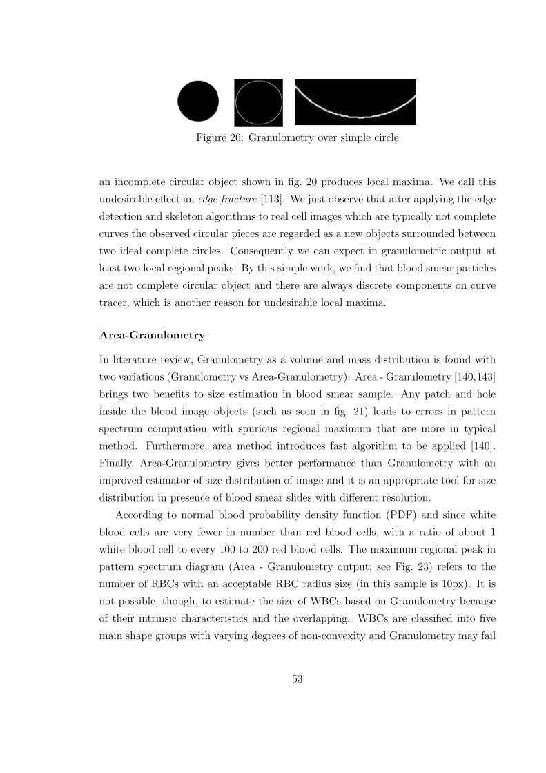
Figure 20: Granulometry over simple circle
an incomplete circular object shown in fig. 20 produces local maxima. We call this
undesirable effect an edge fracture [113]. We just observe that after applying the edge
detection and skeleton algorithms to real cell images which are typically not complete
curves the observed circular pieces are regarded as a new objects surrounded between
two ideal complete circles. Consequently we can expect in granulometric output at
least two local regional peaks. By this simple work, we find that blood smear particles
are not complete circular object and there are always discrete components on curve
tracer, which is another reason for undesirable local maxima.
Area-Granulometry
In literature review, Granulometry as a volume and mass distribution is found with
two variations (Granulometry vs Area-Granulometry). Area - Granulometry [140,143]
brings two benefits to size estimation in blood smear sample. Any patch and hole
inside the blood image objects (such as seen in fig. 21) leads to errors in pattern
spectrum computation with spurious regional maximum that are more in typical
method. Furthermore, area method introduces fast algorithm to be applied [140].
Finally, Area-Granulometry gives better performance than Granulometry with an
improved estimator of size distribution of image and it is an appropriate tool for size
distribution in presence of blood smear slides with different resolution.
According to normal blood probability density function (PDF) and since white
blood cells are very fewer in number than red blood cells, with a ratio of about 1
white blood cell to every 100 to 200 red blood cells. The maximum regional peak in
pattern spectrum diagram (Area - Granulometry output; see Fig. 23) refers to the
number of RBCs with an acceptable RBC radius size (in this sample is 10px). It is
not possible, though, to estimate the size of WBCs based on Granulometry because
of their intrinsic characteristics and the overlapping. WBCs are classified into five
main shape groups with varying degrees of non-convexity and Granulometry may fail
53
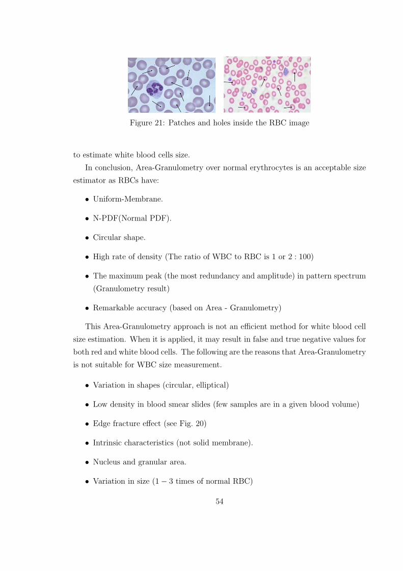
Figure 21: Patches and holes inside the RBC image
to estimate white blood cells size.
In conclusion, Area-Granulometry over normal erythrocytes is an acceptable size
estimator as RBCs have:
• Uniform-Membrane.
• N-PDF(Normal PDF).
• Circular shape.
• High rate of density (The ratio of WBC to RBC is 1 or 2 : 100)
• The maximum peak (the most redundancy and amplitude) in pattern spectrum
(Granulometry result)
• Remarkable accuracy (based on Area - Granulometry)
This Area-Granulometry approach is not an efficient method for white blood cell
size estimation. When it is applied, it may result in false and true negative values for
both red and white blood cells. The following are the reasons that Area-Granulometry
is not suitable for WBC size measurement.
• Variation in shapes (circular, elliptical)
• Low density in blood smear slides (few samples are in a given blood volume)
• Edge fracture effect (see Fig. 20)
• Intrinsic characteristics (not solid membrane).
• Nucleus and granular area.
• Variation in size (1− 3 times of normal RBC)
54
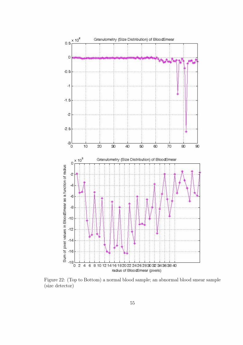
Figure 22: (Top to Bottom) a normal blood sample; an abnormal blood smear sample(size detector)
55
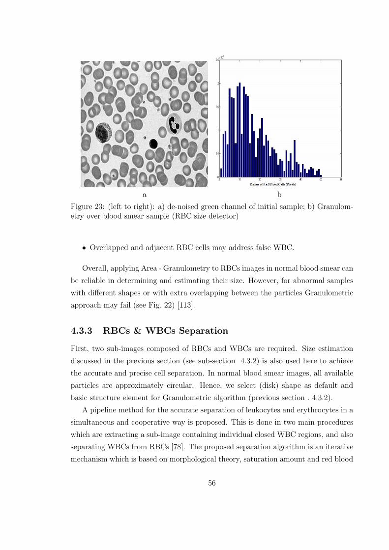
a b
Figure 23: (left to right): a) de-noised green channel of initial sample; b) Granulom-etry over blood smear sample (RBC size detector)
• Overlapped and adjacent RBC cells may address false WBC.
Overall, applying Area - Granulometry to RBCs images in normal blood smear can
be reliable in determining and estimating their size. However, for abnormal samples
with different shapes or with extra overlapping between the particles Granulometric
approach may fail (see Fig. 22) [113].
4.3.3 RBCs & WBCs Separation
First, two sub-images composed of RBCs and WBCs are required. Size estimation
discussed in the previous section (see sub-section 4.3.2) is also used here to achieve
the accurate and precise cell separation. In normal blood smear images, all available
particles are approximately circular. Hence, we select (disk) shape as default and
basic structure element for Granulometric algorithm (previous section . 4.3.2).
A pipeline method for the accurate separation of leukocytes and erythrocytes in a
simultaneous and cooperative way is proposed. This is done in two main procedures
which are extracting a sub-image containing individual closed WBC regions, and also
separating WBCs from RBCs [78]. The proposed separation algorithm is an iterative
mechanism which is based on morphological theory, saturation amount and red blood
56
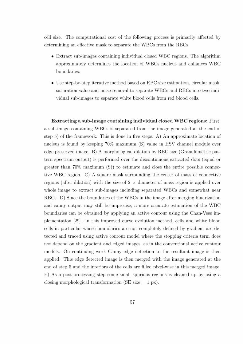
cell size. The computational cost of the following process is primarily affected by
determining an effective mask to separate the WBCs from the RBCs.
• Extract sub-images containing individual closed WBC regions. The algorithm
approximately determines the location of WBCs nucleus and enhances WBC
boundaries.
• Use step-by-step iterative method based on RBC size estimation, circular mask,
saturation value and noise removal to separate WBCs and RBCs into two indi-
vidual sub-images to separate white blood cells from red blood cells.
Extracting a sub-image containing individual closed WBC regions: First,
a sub-image containing WBCs is separated from the image generated at the end of
step 5) of the framework. This is done in five steps: A) An approximate location of
nucleus is found by keeping 70% maximum (S) value in HSV channel module over
edge preserved image. B) A morphological dilation by RBC size (Granulometric pat-
tern spectrum output) is performed over the discontinuous extracted dots (equal or
greater than 70% maximum (S)) to estimate and close the entire possible connec-
tive WBC region. C) A square mask surrounding the center of mass of connective
regions (after dilation) with the size of 2 × diameter of mass region is applied over
whole image to extract sub-images including separated WBCs and somewhat near
RBCs. D) Since the boundaries of the WBCs in the image after merging binarization
and canny output may still be imprecise, a more accurate estimation of the WBC
boundaries can be obtained by applying an active contour using the Chan-Vese im-
plementation [29]. In this improved curve evolution method, cells and white blood
cells in particular whose boundaries are not completely defined by gradient are de-
tected and traced using active contour model where the stopping criteria term does
not depend on the gradient and edged images, as in the conventional active contour
models. On continuing work Canny edge detection to the resultant image is then
applied. This edge detected image is then merged with the image generated at the
end of step 5 and the interiors of the cells are filled pixel-wise in this merged image.
E) As a post-processing step some small spurious regions is cleaned up by using a
closing morphological transformation (SE size = 1 px).
57
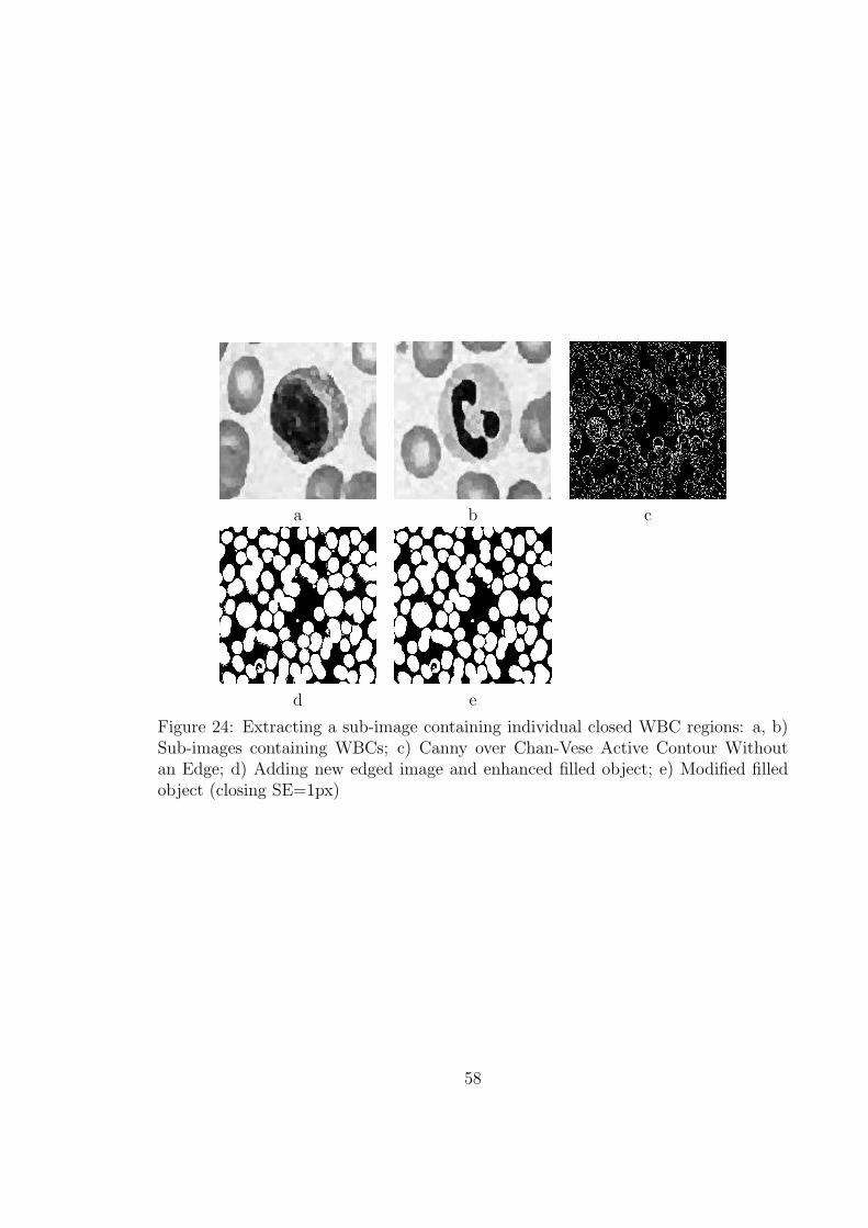
a b c
d e
Figure 24: Extracting a sub-image containing individual closed WBC regions: a, b)Sub-images containing WBCs; c) Canny over Chan-Vese Active Contour Withoutan Edge; d) Adding new edged image and enhanced filled object; e) Modified filledobject (closing SE=1px)
58
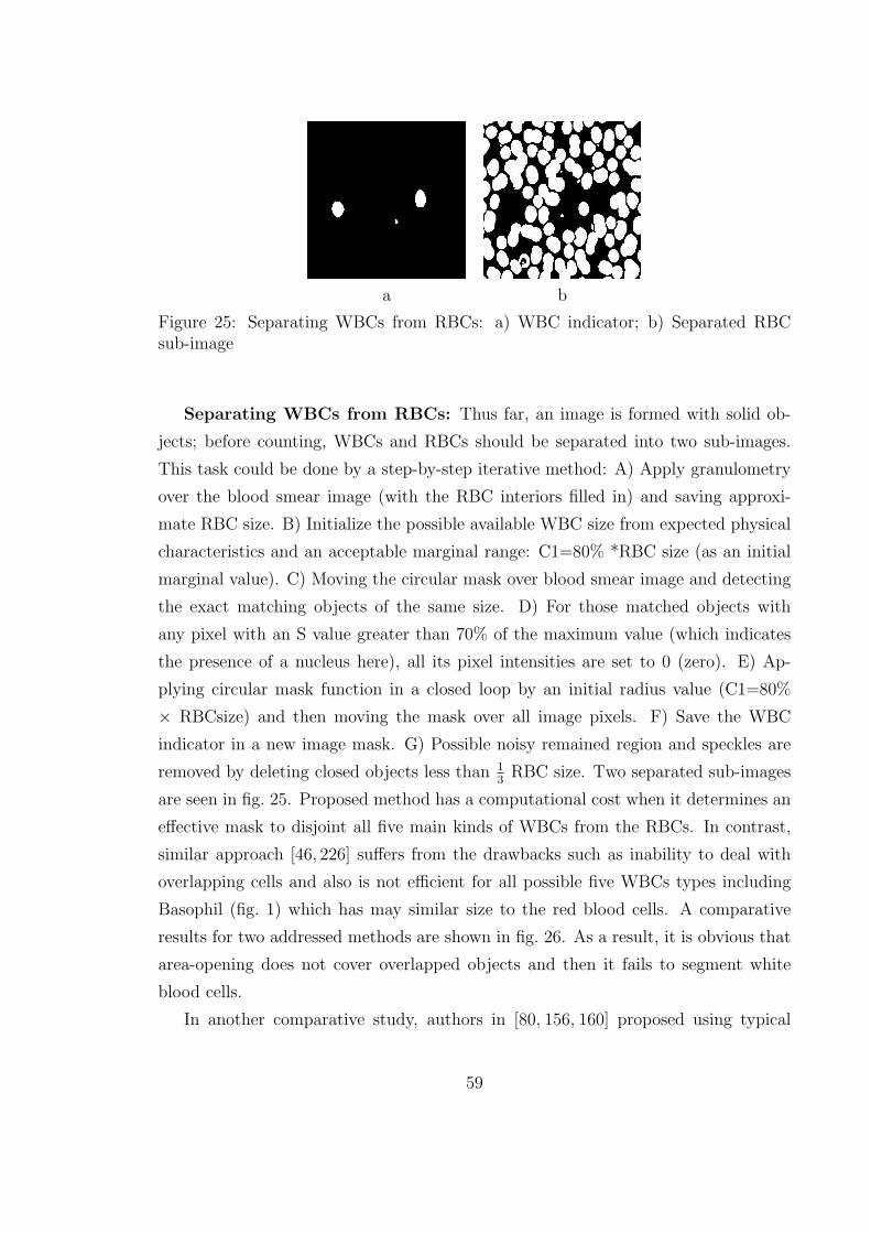
a b
Figure 25: Separating WBCs from RBCs: a) WBC indicator; b) Separated RBCsub-image
Separating WBCs from RBCs: Thus far, an image is formed with solid ob-
jects; before counting, WBCs and RBCs should be separated into two sub-images.
This task could be done by a step-by-step iterative method: A) Apply granulometry
over the blood smear image (with the RBC interiors filled in) and saving approxi-
mate RBC size. B) Initialize the possible available WBC size from expected physical
characteristics and an acceptable marginal range: C1=80% *RBC size (as an initial
marginal value). C) Moving the circular mask over blood smear image and detecting
the exact matching objects of the same size. D) For those matched objects with
any pixel with an S value greater than 70% of the maximum value (which indicates
the presence of a nucleus here), all its pixel intensities are set to 0 (zero). E) Ap-
plying circular mask function in a closed loop by an initial radius value (C1=80%
× RBCsize) and then moving the mask over all image pixels. F) Save the WBC
indicator in a new image mask. G) Possible noisy remained region and speckles are
removed by deleting closed objects less than 13RBC size. Two separated sub-images
are seen in fig. 25. Proposed method has a computational cost when it determines an
effective mask to disjoint all five main kinds of WBCs from the RBCs. In contrast,
similar approach [46, 226] suffers from the drawbacks such as inability to deal with
overlapping cells and also is not efficient for all possible five WBCs types including
Basophil (fig. 1) which has may similar size to the red blood cells. A comparative
results for two addressed methods are shown in fig. 26. As a result, it is obvious that
area-opening does not cover overlapped objects and then it fails to segment white
blood cells.
In another comparative study, authors in [80, 156, 160] proposed using typical
59
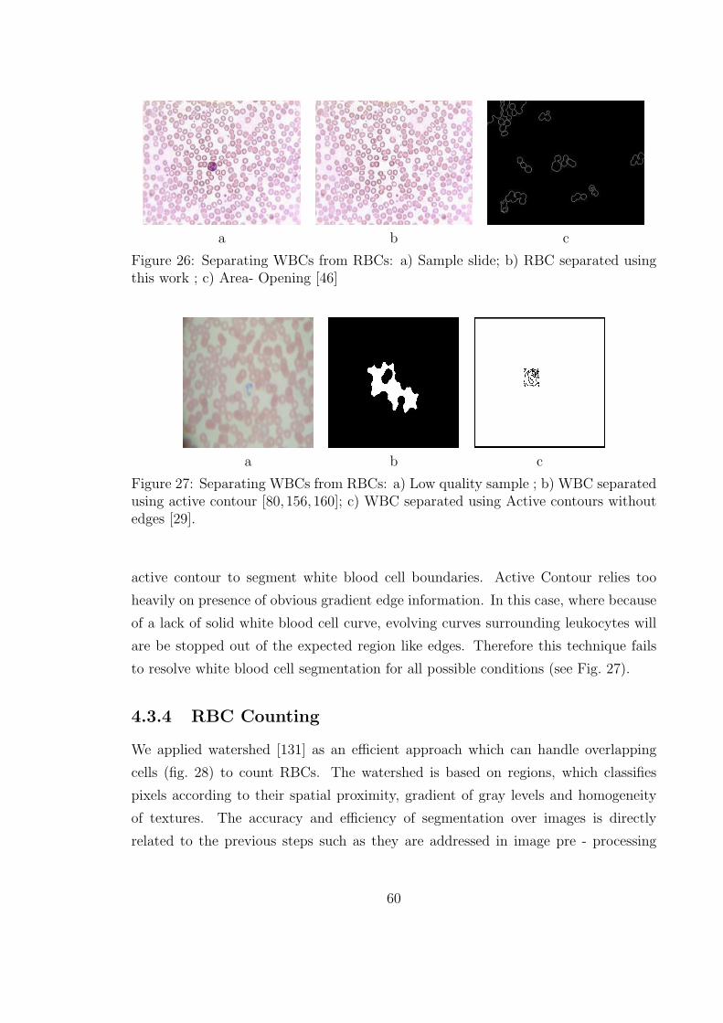
a b c
Figure 26: Separating WBCs from RBCs: a) Sample slide; b) RBC separated usingthis work ; c) Area- Opening [46]
a b c
Figure 27: Separating WBCs from RBCs: a) Low quality sample ; b) WBC separatedusing active contour [80, 156, 160]; c) WBC separated using Active contours withoutedges [29].
active contour to segment white blood cell boundaries. Active Contour relies too
heavily on presence of obvious gradient edge information. In this case, where because
of a lack of solid white blood cell curve, evolving curves surrounding leukocytes will
are be stopped out of the expected region like edges. Therefore this technique fails
to resolve white blood cell segmentation for all possible conditions (see Fig. 27).
4.3.4 RBC Counting
We applied watershed [131] as an efficient approach which can handle overlapping
cells (fig. 28) to count RBCs. The watershed is based on regions, which classifies
pixels according to their spatial proximity, gradient of gray levels and homogeneity
of textures. The accuracy and efficiency of segmentation over images is directly
related to the previous steps such as they are addressed in image pre - processing
60
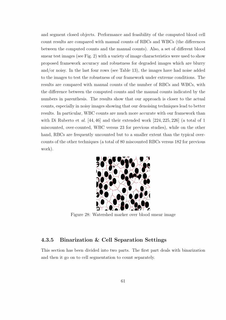
and segment closed objects. Performance and feasibility of the computed blood cell
count results are compared with manual counts of RBCs and WBCs (the differences
between the computed counts and the manual counts). Also, a set of different blood
smear test images (see Fig. 2) with a variety of image characteristics were used to show
proposed framework accuracy and robustness for degraded images which are blurry
and/or noisy. In the last four rows (see Table 13), the images have had noise added
to the images to test the robustness of our framework under extreme conditions. The
results are compared with manual counts of the number of RBCs and WBCs, with
the difference between the computed counts and the manual counts indicated by the
numbers in parenthesis. The results show that our approach is closer to the actual
counts, especially in noisy images showing that our denoising techniques lead to better
results. In particular, WBC counts are much more accurate with our framework than
with Di Ruberto et al. [44, 46] and their extended work [224, 225, 226] (a total of 1
miscounted, over-counted, WBC versus 23 for previous studies), while on the other
hand, RBCs are frequently uncounted but to a smaller extent than the typical over-
counts of the other techniques (a total of 80 miscounted RBCs versus 182 for previous
work).
Figure 28: Watershed marker over blood smear image
4.3.5 Binarization & Cell Separation Settings
This section has been divided into two parts. The first part deals with binarization
and then it go on to cell segmentation to count separately.
61
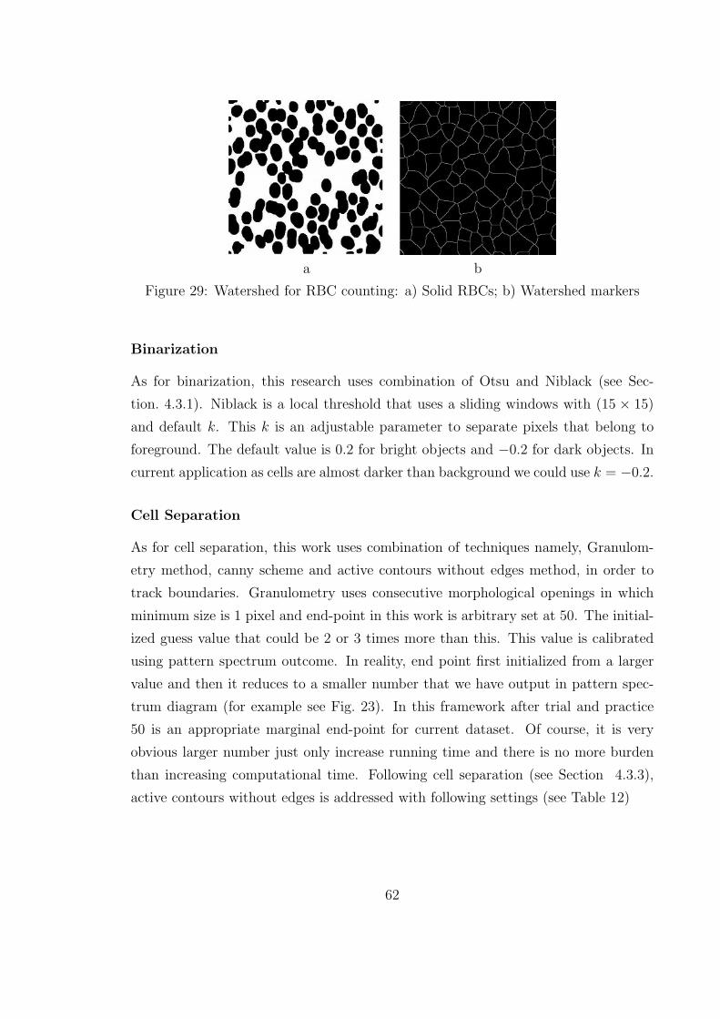
a b
Figure 29: Watershed for RBC counting: a) Solid RBCs; b) Watershed markers
Binarization
As for binarization, this research uses combination of Otsu and Niblack (see Sec-
tion. 4.3.1). Niblack is a local threshold that uses a sliding windows with (15 × 15)
and default k. This k is an adjustable parameter to separate pixels that belong to
foreground. The default value is 0.2 for bright objects and −0.2 for dark objects. In
current application as cells are almost darker than background we could use k = −0.2.
Cell Separation
As for cell separation, this work uses combination of techniques namely, Granulom-
etry method, canny scheme and active contours without edges method, in order to
track boundaries. Granulometry uses consecutive morphological openings in which
minimum size is 1 pixel and end-point in this work is arbitrary set at 50. The initial-
ized guess value that could be 2 or 3 times more than this. This value is calibrated
using pattern spectrum outcome. In reality, end point first initialized from a larger
value and then it reduces to a smaller number that we have output in pattern spec-
trum diagram (for example see Fig. 23). In this framework after trial and practice
50 is an appropriate marginal end-point for current dataset. Of course, it is very
obvious larger number just only increase running time and there is no more burden
than increasing computational time. Following cell separation (see Section 4.3.3),
active contours without edges is addressed with following settings (see Table 12)
62
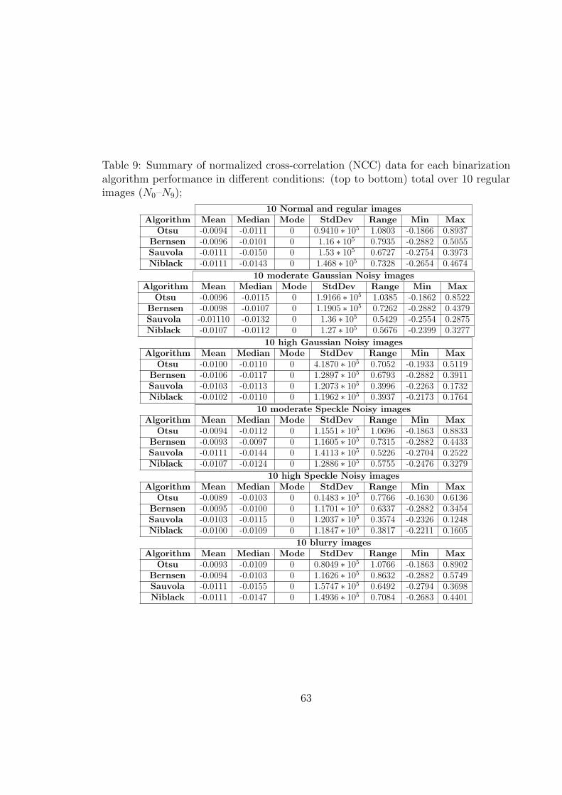
Table 9: Summary of normalized cross-correlation (NCC) data for each binarizationalgorithm performance in different conditions: (top to bottom) total over 10 regularimages (N0–N9);
10 Normal and regular imagesAlgorithm Mean Median Mode StdDev Range Min Max
Otsu -0.0094 -0.0111 0 0.9410 ∗ 105 1.0803 -0.1866 0.8937Bernsen -0.0096 -0.0101 0 1.16 ∗ 105 0.7935 -0.2882 0.5055Sauvola -0.0111 -0.0150 0 1.53 ∗ 105 0.6727 -0.2754 0.3973Niblack -0.0111 -0.0143 0 1.468 ∗ 105 0.7328 -0.2654 0.4674
10 moderate Gaussian Noisy imagesAlgorithm Mean Median Mode StdDev Range Min Max
Otsu -0.0096 -0.0115 0 1.9166 ∗ 105 1.0385 -0.1862 0.8522Bernsen -0.0098 -0.0107 0 1.1905 ∗ 105 0.7262 -0.2882 0.4379Sauvola -0.01110 -0.0132 0 1.36 ∗ 105 0.5429 -0.2554 0.2875Niblack -0.0107 -0.0112 0 1.27 ∗ 105 0.5676 -0.2399 0.3277
10 high Gaussian Noisy imagesAlgorithm Mean Median Mode StdDev Range Min Max
Otsu -0.0100 -0.0110 0 4.1870 ∗ 105 0.7052 -0.1933 0.5119Bernsen -0.0106 -0.0117 0 1.2897 ∗ 105 0.6793 -0.2882 0.3911Sauvola -0.0103 -0.0113 0 1.2073 ∗ 105 0.3996 -0.2263 0.1732Niblack -0.0102 -0.0110 0 1.1962 ∗ 105 0.3937 -0.2173 0.1764
10 moderate Speckle Noisy imagesAlgorithm Mean Median Mode StdDev Range Min Max
Otsu -0.0094 -0.0112 0 1.1551 ∗ 105 1.0696 -0.1863 0.8833Bernsen -0.0093 -0.0097 0 1.1605 ∗ 105 0.7315 -0.2882 0.4433Sauvola -0.0111 -0.0144 0 1.4113 ∗ 105 0.5226 -0.2704 0.2522Niblack -0.0107 -0.0124 0 1.2886 ∗ 105 0.5755 -0.2476 0.3279
10 high Speckle Noisy imagesAlgorithm Mean Median Mode StdDev Range Min Max
Otsu -0.0089 -0.0103 0 0.1483 ∗ 105 0.7766 -0.1630 0.6136Bernsen -0.0095 -0.0100 0 1.1701 ∗ 105 0.6337 -0.2882 0.3454Sauvola -0.0103 -0.0115 0 1.2037 ∗ 105 0.3574 -0.2326 0.1248Niblack -0.0100 -0.0109 0 1.1847 ∗ 105 0.3817 -0.2211 0.1605
10 blurry imagesAlgorithm Mean Median Mode StdDev Range Min Max
Otsu -0.0093 -0.0109 0 0.8049 ∗ 105 1.0766 -0.1863 0.8902Bernsen -0.0094 -0.0103 0 1.1626 ∗ 105 0.8632 -0.2882 0.5749Sauvola -0.0111 -0.0155 0 1.5747 ∗ 105 0.6492 -0.2794 0.3698Niblack -0.0111 -0.0147 0 1.4936 ∗ 105 0.7084 -0.2683 0.4401
63
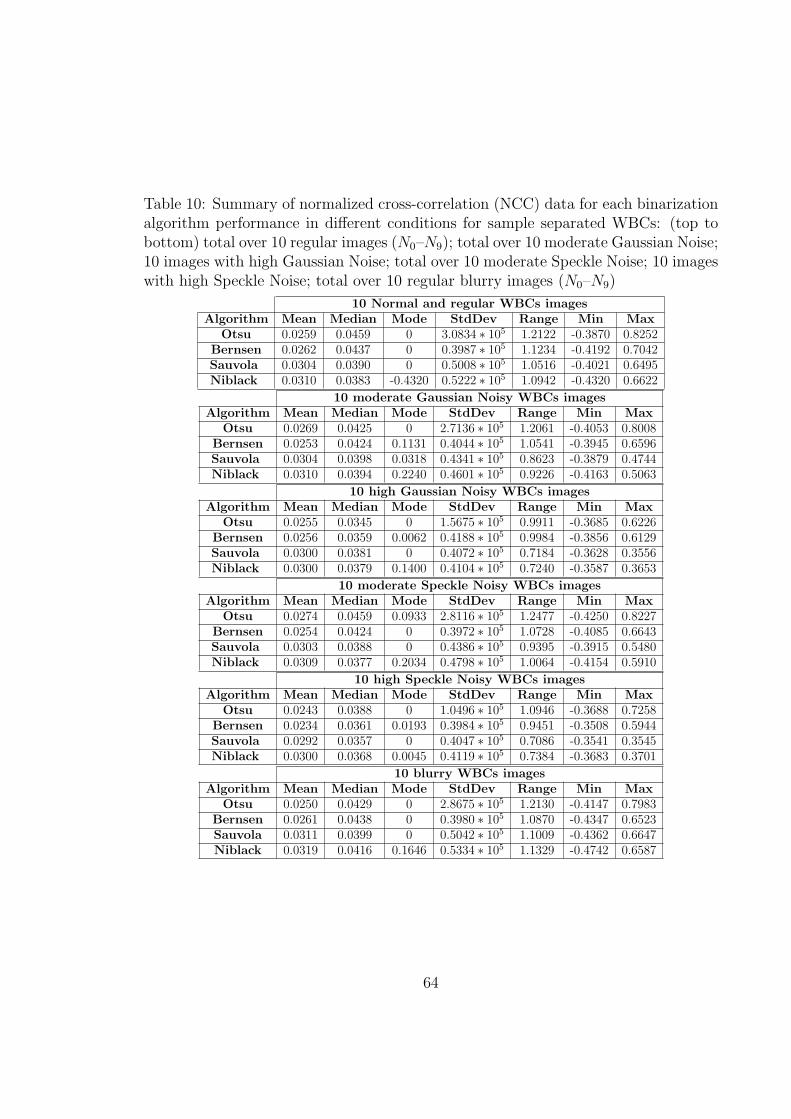
Table 10: Summary of normalized cross-correlation (NCC) data for each binarizationalgorithm performance in different conditions for sample separated WBCs: (top tobottom) total over 10 regular images (N0–N9); total over 10 moderate Gaussian Noise;10 images with high Gaussian Noise; total over 10 moderate Speckle Noise; 10 imageswith high Speckle Noise; total over 10 regular blurry images (N0–N9)
10 Normal and regular WBCs imagesAlgorithm Mean Median Mode StdDev Range Min Max
Otsu 0.0259 0.0459 0 3.0834 ∗ 105 1.2122 -0.3870 0.8252Bernsen 0.0262 0.0437 0 0.3987 ∗ 105 1.1234 -0.4192 0.7042Sauvola 0.0304 0.0390 0 0.5008 ∗ 105 1.0516 -0.4021 0.6495Niblack 0.0310 0.0383 -0.4320 0.5222 ∗ 105 1.0942 -0.4320 0.6622
10 moderate Gaussian Noisy WBCs imagesAlgorithm Mean Median Mode StdDev Range Min Max
Otsu 0.0269 0.0425 0 2.7136 ∗ 105 1.2061 -0.4053 0.8008Bernsen 0.0253 0.0424 0.1131 0.4044 ∗ 105 1.0541 -0.3945 0.6596Sauvola 0.0304 0.0398 0.0318 0.4341 ∗ 105 0.8623 -0.3879 0.4744Niblack 0.0310 0.0394 0.2240 0.4601 ∗ 105 0.9226 -0.4163 0.5063
10 high Gaussian Noisy WBCs imagesAlgorithm Mean Median Mode StdDev Range Min Max
Otsu 0.0255 0.0345 0 1.5675 ∗ 105 0.9911 -0.3685 0.6226Bernsen 0.0256 0.0359 0.0062 0.4188 ∗ 105 0.9984 -0.3856 0.6129Sauvola 0.0300 0.0381 0 0.4072 ∗ 105 0.7184 -0.3628 0.3556Niblack 0.0300 0.0379 0.1400 0.4104 ∗ 105 0.7240 -0.3587 0.3653
10 moderate Speckle Noisy WBCs imagesAlgorithm Mean Median Mode StdDev Range Min Max
Otsu 0.0274 0.0459 0.0933 2.8116 ∗ 105 1.2477 -0.4250 0.8227Bernsen 0.0254 0.0424 0 0.3972 ∗ 105 1.0728 -0.4085 0.6643Sauvola 0.0303 0.0388 0 0.4386 ∗ 105 0.9395 -0.3915 0.5480Niblack 0.0309 0.0377 0.2034 0.4798 ∗ 105 1.0064 -0.4154 0.5910
10 high Speckle Noisy WBCs imagesAlgorithm Mean Median Mode StdDev Range Min Max
Otsu 0.0243 0.0388 0 1.0496 ∗ 105 1.0946 -0.3688 0.7258Bernsen 0.0234 0.0361 0.0193 0.3984 ∗ 105 0.9451 -0.3508 0.5944Sauvola 0.0292 0.0357 0 0.4047 ∗ 105 0.7086 -0.3541 0.3545Niblack 0.0300 0.0368 0.0045 0.4119 ∗ 105 0.7384 -0.3683 0.3701
10 blurry WBCs imagesAlgorithm Mean Median Mode StdDev Range Min Max
Otsu 0.0250 0.0429 0 2.8675 ∗ 105 1.2130 -0.4147 0.7983Bernsen 0.0261 0.0438 0 0.3980 ∗ 105 1.0870 -0.4347 0.6523Sauvola 0.0311 0.0399 0 0.5042 ∗ 105 1.1009 -0.4362 0.6647Niblack 0.0319 0.0416 0.1646 0.5334 ∗ 105 1.1329 -0.4742 0.6587
64
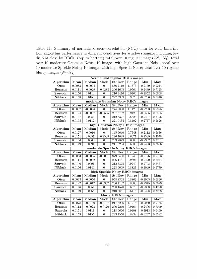
Table 11: Summary of normalized cross-correlation (NCC) data for each binariza-tion algorithm performance in different conditions for windows sample including fewdisjoint close by RBCs: (top to bottom) total over 10 regular images (N0–N9); totalover 10 moderate Gaussian Noise; 10 images with high Gaussian Noise; total over10 moderate Speckle Noise; 10 images with high Speckle Noise; total over 10 regularblurry images (N0–N9)
Normal and regular RBCs imagesAlgorithm Mean Median Mode StdDev Range Min Max
Otsu 0.0083 -0.0094 0 886.7119 1.1373 -0.2159 0.9214Bernsen 0.0111 -0.0029 -0.0283 206.1605 0.9564 -0.2439 0.7125Sauvola 0.0150 0.0114 0 216.3476 0.9460 -0.2852 0.6608Niblack 0.0158 0.0153 0 227.5969 0.9023 -0.3206 0.5816
moderate Gaussian Noisy RBCs imagesAlgorithm Mean Median Mode StdDev Range Min Max
Otsu 0.0087 -0.0094 0 774.9890 1.1128 -0.2203 0.8925Bernsen 0.0124 -0.0007 -0.2535 207.6752 0.9120 -0.2535 0.6585Sauvola 0.0147 0.0084 0 212.8327 0.8623 -0.2497 0.6126Niblack 0.0155 0.0112 0 221.0434 0.8402 -0.2777 0.5626
high Gaussian Noisy RBCs imagesAlgorithm Mean Median Mode StdDev Range Min Max
Otsu 0.0127 -0.0010 0 145.6640 0.7748 -0.2112 0.5636Bernsen 0.0151 0.0057 -0.2599 226.7028 0.6677 -0.2599 0.4078Sauvola 0.0146 0.0068 0 209.7879 0.6003 -0.2302 0.3701Niblack 0.0149 0.0091 0 211.5264 0.6039 -0.2403 0.3636
moderate Speckle Noisy RBCs imagesAlgorithm Mean Median Mode StdDev Range Min Max
Otsu 0.0083 -0.0095 -0.0061 879.6408 1.1249 -0.2126 0.9123Bernsen 0.0111 -0.0032 0 206.1431 0.9394 -0.2420 0.6974Sauvola 0.0146 0.0091 0 212.3325 0.9249 -0.2798 0.6451Niblack 0.0156 0.0140 0 223.6009 0.8827 -0.3049 0.5779
high Speckle Noisy RBCs imagesAlgorithm Mean Median Mode StdDev Range Min Max
Otsu 0.0093 -0.0050 0 958.8368 0.8862 -0.1965 0.6896Bernsen 0.0122 -0.0017 -0.0307 206.7132 0.8003 -0.2375 0.5629Sauvola 0.0146 0.0054 0 208.1570 0.6578 -0.2358 0.4220Niblack 0.0149 0.0068 0 210.8861 0.6416 -0.2428 0.3988
blurry RBCs imagesAlgorithm Mean Median Mode StdDev Range Min Max
Otsu 0.0078 -0.0100 -0.0107 917.8296 1.1215 -0.2050 0.9165Bernsen 0.0112 -0.0023 -0.0470 206.2240 0.9465 -0.2406 0.7059Sauvola 0.0151 0.0111 0 218.9666 0.9408 -0.2918 0.6490Niblack 0.0159 0.0155 0 233.7550 0.8839 -0.3247 0.5592
65

Table 12: Boundaries detection: Settings
Active contours without edgesParameter Value Comment
Mask Small Create a small circular mask to track gradient.NumIter 1500 Total number of iterations that is a trade-off between
computational complexity and contour accuracy.Mu 0.1 Weight of length term.
Method Multi phase 2-phase segmentation of the image is applied to detectboth contours with, or without gradient.
66
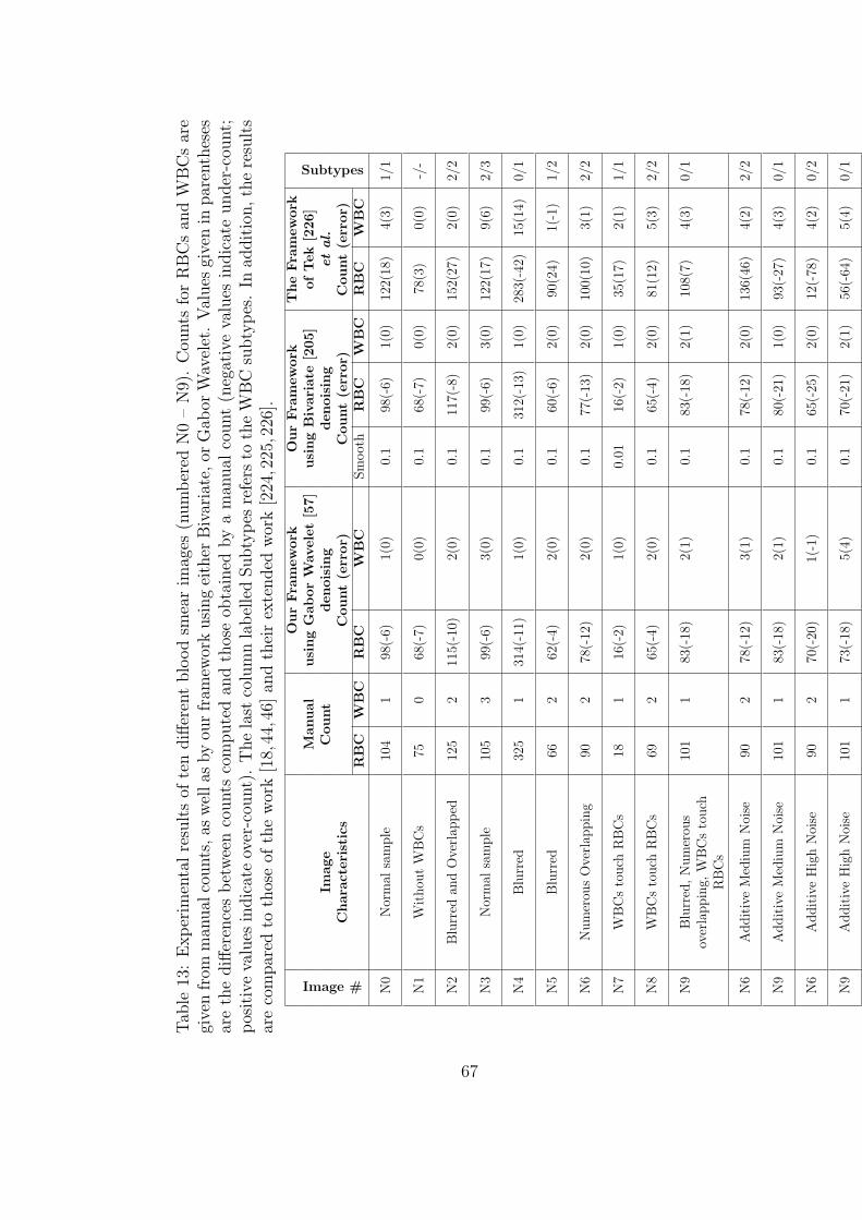
Tab
le13:Experim
entalresultsof
tendifferentbloodsm
earim
ages
(numbered
N0–N9).Cou
nts
forRBCsan
dW
BCsare
givenfrom
man
ual
counts,as
wellas
byou
rfram
eworkusingeither
Bivariate,or
Gab
orWavelet.Values
givenin
parentheses
arethedifferencesbetweencounts
computedan
dthoseob
tained
byaman
ual
count(negativevalues
indicateunder-cou
nt;
positivevalues
indicateover-cou
nt).Thelast
columnlabelledSubtypes
refers
totheW
BCsubtypes.In
addition,theresults
arecompared
tothoseof
thework[18,44,46]
andtheirextended
work[224,225,226].
Image #
Ou
rFra
mew
ork
Ou
rFra
mew
ork
Th
eFra
mew
ork
Subtypes
Manu
al
usi
ng
Gab
or
Wavele
t[5
7]
usi
ng
Biv
ari
ate
[205]
of
Tek
[226]
Image
Cou
nt
den
ois
ing
den
ois
ing
etal.
Ch
ara
cteri
stic
sC
ou
nt
(err
or)
Cou
nt
(err
or)
Cou
nt
(err
or)
RB
CW
BC
RB
CW
BC
Smooth
RB
CW
BC
RB
CW
BC
N0
Normal
sample
104
198(-6)
1(0)
0.1
98(-6)
1(0)
122(18)
4(3)
1/1
N1
Withou
tW
BCs
750
68(-7)
0(0)
0.1
68(-7)
0(0)
78(3)
0(0)
-/-
N2
Blurred
andOv erlap
ped
125
2115(-10)
2(0)
0.1
117(-8)
2(0)
152(27)
2(0)
2/2
N3
Normal
sample
105
399(-6)
3(0)
0.1
99(-6)
3(0)
122(17)
9(6)
2/3
N4
Blurred
325
1314(-11)
1(0)
0.1
312(-13)
1(0)
283(-42)
15(14)
0/1
N5
Blurred
662
62(-4)
2(0)
0.1
60(-6)
2(0)
90(24)
1(-1)
1/2
N6
Numerou
sOverlap
ping
902
78(-12)
2(0)
0.1
77(-13)
2(0)
100(10)
3(1)
2/2
N7
WBCstouch
RBCs
181
16(-2)
1(0)
0.01
16(-2)
1(0)
35(17)
2(1)
1/1
N8
WBCstouch
RBCs
692
65(-4)
2(0)
0.1
65(-4)
2(0)
81(12)
5(3)
2/2
N9
Blurred,Numerou
soverlapping,
WBCstouch
RBCs
101
183(-18)
2(1)
0.1
83(-18)
2(1)
108(7)
4(3)
0/1
N6
AdditiveMedium
Noise
902
78(-12)
3(1)
0.1
78(-12)
2(0)
136(46)
4(2)
2/2
N9
AdditiveMedium
Noise
101
183(-18)
2(1)
0.1
80(-21)
1(0)
93(-27)
4(3)
0/1
N6
AdditiveHighNoise
902
70(-20)
1(-1)
0.1
65(-25)
2(0)
12(-78)
4(2)
0/2
N9
AdditiveHighNoise
101
173(-18)
5(4)
0.1
70(-21)
2(1)
56(-64)
5(4)
0/1
67
4.4 Comparison of the Proposed Approach to the
State-of-the-Art
Comparative studies on state-of-the-art are divided into binarization and blood cell
segmentation.
4.4.1 Binarization
To date, the blood smear studies are more about global thresholding methods than
local thresholding methods. Published work on blood segmentation [15,44,46,224,225,
226,242] use well-known Otsu global thresholding approach. The existing global Otsu
thresholding value fails to resolve different conditions that exist in blood slide images.
Inconsistent initial conditions may cause an abrupt change in global thresholding
value and the binarization cannot construct a consistent system of foreground and
background separation. Finding a global value as thresholding to separate the image
into two separated regions of blood cells (RBCs in particular) and background (stained
plasma) is not always simple and perhaps not even possible. It may cause false
negative (FN) result in foreground detection (see Table 13). Global thresholding is
with a serious weakness, however, is that much known but also it does not manage
image binarization with nearby background and foreground intensity values range
(see Fig. 19). Closely positioned pairs of particles will be merged into single particles,
regardless of any fine tuning of the value of global thresholding. It is obvious that
merged cells may cause false negative (FN) in RBCs detection (see Fig. 19). Overall,
Otsu is a parameterless method to remove background details such as found in stained
plasma background. However, it is non-adaptive to retain cells as they are foreground.
This work suggests to use combination of global and local thresholding to reach
higher similarities between original and binarized converted images ( see Table. 11).
Merging Otsu and Niblack alleviates built-in problems in presence of adjacent cells
and background variety.
4.4.2 Cell Separation
In an important work Di Ruberto et al. [44,46] and their extended work [224,225,226]
authors addressed classical area opening morphology technique to separate between
68
WBCs and RBCs. Authors claimed that white blood cells can be separated by a
morphological erosion with a disk-shaped structuring element whose size is achieved
by the granulometric analysis (RBC size). Despite the simplicity of implementation
and understanding, proposed method suffers from several major drawbacks. First, all
white blood cells are not always bigger than a normal RBC size as Basophil which
is about RBC size (see 4th image in top row in fig. 10). Secondly, overlapping phe-
nomena among cells is also possible and it is a normal incident in blood smear slides.
Therefore, these work findings cannot be extrapolated to all sample slides and these
results therefore need to be interpreted with caution. A generally accepted framework
of cell segmentation is lacking (see Fig. 26). Other work [80, 156, 160] addresses to
use nucleus and its surrounding active contour and level set to separate WBCs in
which generalization of these methods are very questionable in different conditions.
First and foremost weakness backs to regular nature of leukocyte boundaries, lack
of obvious edge for WBCs and low quality in nucleus presentation. In the classical
active contour models an edge-detector is highly used to stop the evolving curve on
the boundary of the desired white blood cell. However, WBC boundaries are not ide-
ally defined by gradient in low quality images and it easily make false segmentation
(see Fig. 27). Secondly, initial contour location is needed and should be close to the
white blood cell that is to be segmented. Authors in [208] proposed fuzzy cellular
neural networks (FCNN) to detect white blood cell. The principal are combination
of fuzzy logic, and neural networks. Neural network uses enough number of different
samples to give optimal generalization and update properties of back-propagation.
This approach is not practical with this limited available dataset, i.e. 28 samples per
each white blood cell class. In practice, having big data is not easy to address in
medical projects.
This research is dealing with blood smear images segmentation using a step-by-
step iterative method. More information is addressed in section 4.3.3. This frame-
work can be extrapolated to all five mature white blood cells including Basophils.
This step-by-step method managed faded white blood cell boundaries in this difficult
dataset with active contours without edges and canny detection on top of that. It
built a closed curve delineating a white blood cell despite of detecting these edges in
other work [80, 156, 160]. It also managed overlapping incident that is common be-
tween RBCs in particular. However, it should be noted that the method and results
69
presented here in this work are only applicable for normal microscopic blood images.
This algorithm may fails in presence of abnormal conditions such as Malaria.
4.5 Binarization & Cell Separation Contributions
Another contribution is the procedure developed for obtaining optimum binary im-
ages from mono-chromic channel with inhomogeneous background regions by creating
a merged local and global binarization. This procedure is efficient and promising for
all types of captured blood images with different conditions. This binarization al-
gorithm is an important improvement as the previous work in this field used global
thresholding approaches, i.e. Otsu, that these global findings cannot be extrapolated
to all possible blood smear images (see Section 4.4.1). In addition, the study has
gone some way towards enhancing our understanding of faded boundaries problem
in white blood cell separation (see sub-section 4.3.3 and figure 27). Taken together,
these findings suggest a role for active contours without edges in white blood cell
segmentation for all classes.
4.5.1 Binarization
To date, the blood smear researches are more about on global thresholding methods
rather than local thresholding methods. This work addresses to use combination of
global and local thresholding to reach higher similarities between original and bina-
rized converted images. The missing cells in global approach is enhanced using this
merged technique, for which the local thresholding gives the required foreground as
cells. The method used for this blood smear study may be applied to other histopatho-
logical images also. Comparative study and discussion is found in section 4.4.1 and
figure 19.
4.5.2 Cell Separation
This research is dealing with blood smear images segmentation using a step-by-step
iterative method. White blood cells are localized and segmented with reference to
improved binarization, edge detection, saturation value, RBC size estimation, cir-
cular morphological mask, active contours without edges, and noise removal. More
70
information is addressed in section. 4.3.3. This framework can be extrapolated to all
five mature white blood cells including Basophils. This step-by-step method man-
aged faded white blood cell boundaries in this difficult dataset with active contours
without edges and canny detection on top of that. It built a closed curve delineating
a white blood cell despite of detecting these edges in other work [80,156,160]. It also
managed overlapping incident that is common between RBCs in particular.
Comparative studies and discussion is addressed in section 4.4.2. In addition, it
should be noted that the method and results presented here in this work are only
applicable for normal microscopic blood images. This algorithm may fails in presence
of abnormal conditions such as Malaria.
71
Chapter 5
Feature Extraction For WBC
Classification
Image feature extraction has been established for years and has been used in many
diverse pattern recognition and image processing fields. However, choosing efficient
features for the detection of white blood cell from pathological images is significant
problem. The main task of the feature extraction is to choose strongest connected
correlated with the recognized classes. The main goal of feature extraction is to
identify the strong features, i.e., the features with high discriminatory power. The
aforementioned features can be grouped into three categories: shape, intensity, and
texture features.
5.1 Problem Statement
This research aims to improve WBC type recognition even in presence of poor quality
or low magnification images (see Fig. 1). In order to distinguish among white blood
cells types, we need to extract features from the WBC sub-images and compute new
features that lead to better separability of classes by classifiers. Features should
be easily computed, robust, insensitive to various distortions and variations in the
images, and rotationally invariant.
Features Combination:
Combining all individual features together allows to compensate error rates and also
it increases their classification reliability to some extent. Features are generated using
72
different transformation parameters and also are evaluated to select the set with best
discrimination power.
Features Reduction:
To reduce excessive dimensionality of different features, linear or non-linear combi-
nations of features are applied through projection of the high-dimensional data on
lower dimensional space to optimize the accuracy of classifier and it also reduces
computational cost. To maintain the optimal features and components, non-linear
dimensionality reduction methods under different names and algorithms have been
introduced. They include PCA [96], locally linear embedding (LLE) [196] and graph
embedding [254].
Numerous studies have attempted to explain these feature reduction techniques
However, limited work has been able to draw attention to feature selection algorithms.
In this study, we use feature selection algorithms described in section. 6.
5.2 Literature Review
The literature on automatic leukocyte segmentation and classification involves dif-
ferent descriptors and sub-class classification. Section 2.2.2 reviews the literature
concerning white blood cell in connection with different approaches. These stud-
ies are based on active contour, fuzzy logic, morphological operations and feature
extraction.
5.3 Research & Experimental Results
All invariant features are scaled between 0 and 1 to simplify computational complexity
and have consistent inputs for measurement. As a result the final features vector has
a total of 12104 coefficients for each white blood cell image with 28 × 28 low size.
We use feature vector based on three main group features that it includes different
invariant features such as four main intensity histogram calculations, the set of 11
invariant moments, the relative area, the co-occurrence, run-length matrices, the dual
tree complex wavelet transform, Haralick and Tamura features.
73
5.3.1 Intensity Features
The Gray scale intensity values are used to extract efficient features for white blood
cell classification. This work examines the mean (µ), standard deviation (σ), skewness
(γ1), and kurtosis (K) of white blood cells intensities. These features are based only
on the absolute value of the intensity measurements in the segmented white blood
cell images. A histogram describes the occurrence relative frequency of the intensity
values of the pixels in a white blood cell image. The intensity features that we
will consider are the first four central moments of this histogram: Mean, Standard
deviation, Skewness, and Kurtosis [193]. The mean (µ) gives an estimate of the
average intensity level in the region of the cell and the standard deviation (σ) is
a measure of the dispersion of intensity. Skewness (γ1) is a measure of histogram
symmetry while kurtosis (K) is a measure of the tail of the histogram. Intensity
features may prove inadequate for specially low quality white blood cell data set. For
this dataset, other features such as the shape, and texture features may be useful for
improved white blood cell classification.
5.3.2 Shape Features
In image processing and pattern recognition, two types of shape descriptors are
used:contour-based and region-based. The former provides the objects external border
information where they ignore the shape of the interior content. The latter considers
both boundary and the interior of the digital shape.
Several studies investigating contour-based descriptors have been carried out on
different algorithm names. Examples to contour-based shape descriptors includes
chain code algorithm which is the first approach for representing connected external
curves [61]. Other option is Fourier descriptors which exploit shape signatures in
Fourier coefficients. It represents shape in a frequency domain [68,100,171].
The object boundary contours can be also extracted through curvature scale
space [145, 146]. B-spline curve approximation is sum of pixels under a given cri-
terion which optimally approximates the original object curve [70]. Polygon decom-
position is a structural shape representation where boundaries are first sub-divided
into line segments by polygon approximation [169, 202]. Furthermore, a number of
other investigations into the contour-based shape descriptors are also addressed such
as perimeter, compactness (perimeter2
area), eccentricity (a measure of aspect ratio; length
74
of major axis to minor axis), Hausdoff distance (a measure of similarity) [53], and
autoregressive (estimate the image model by prior knowledge) [52].
All these mentioned contour-based descriptors reviewed so far cannot represent
ideally white blood cell shapes for which the complete and continuous boundary
information is not ideally available with granular and non-uniform borders.
Also, questions have been raised about the validity and reliability under the con-
straints of translation, rotation and uniform-scaling invariance properties. Region-
based shape descriptors derive benefit from both boundaries and interior pixels and
that is why it would be an appropriate candidate for white blood cell detection at
low resolution.
Invariant Moment-based Features
In reviewing the literature, the current study found that among different various shape
features are often named, invariant moment as a region-based calculation which can
provide invariant characteristics under different conditions are likely occur. Although
moment algorithms and theory have been well established in mathematics, far too
little attention has been paid to use of invariant moment in computer-aided diagnosis
(CAD) in medical imaging and for blood smear analysis in particular. This research
has given an account the reasons for the widespread use of (11) different invariant
moments (are listed below) over white blood cells images with 28× 28 pixel size.
The Hu set of Invariant Moments:
In the decade 60, a set of seven invariant moments was given by Hu [91, 151].
Shape feature variables computed from normalized centralized non-orthogonal mo-
ments up to order three. Hu set moments are one of the most widely used groups
of invariant moments and have been extensively used for decades in pattern recog-
nition. However, a major problem with this application is information redundancy.
Mathematical terms are defined in [91,151].
These Hu set invariant moments (IM) are invariant to shape changes in rotation,
scaling and translation. It can be used for disjoint objects as well such as granular
white blood cell cytoplasm (non-continuous and discrete borders), 3-4 lobed nucleus
Eosinophil, bilobed nucleus Basophil, partially two lobes Lymphocyte; which are
available in joint or disjoint form and appearance in normal white blood cells. How-
ever, it should be noted that higher-order Hu set moments are sensitive to noise and
75
they suffer from information redundancy.
The Orthogonal Polynomials Moments:
Discrete orthogonal moments (OM) are approaches to lessen information redun-
dancy drawback and shortcomings. Our work will review the research conducted on
the following orthogonal polynomials moments. In reviewing the literature, authors
carried out a number of investigations into using the following invariant moment in
pattern recognition. However, very little was found in the literature on the question
of using moment in medical imaging. Zernike [128], Generalized Pseudo-Zernike [250],
Fourier-Chebyshev [172], Fourier-Mellin [207], Radial Harmonic Fourier [187], Dual
Hahn which are a complex set of Tchebichef and Krawtchouk moments [108], Discrete
Chebyshev [150], Krawtchouk [256], Gegenbauer [89], Legendre [62, 261] are orthog-
onal moments investigated in our research. A brief comparative study of invariant
moment approaches is summarized in table 14.
Brief review of invariant orthogonal moments in image processing: This section re-
views the literature concerning the usefulness of using moment concepts in pattern
recognition. This review has been divided into eleven parts. The first part deals with
already published work in Zernike moment and then it looks at how other consecutive
ten moments are addressed in literature review.
In recent years, several studies investigating Zernike orthogonal moment have been
carried out on blood smear images. In 2006, Asadi et al. published a paper [9] in which
they described Zernike moments in correspondence with leukemia cell classification.
In 2011, Apostolopoulos et al. [6] pointed to some of the ways in which actual RBC
sizes is estimated using Zernike feature sets with repetition degree n = 6 and different
polynomial orders. In addition, in 2013, Das and co workers [39] demonstrated that
Zernike features propose shape-based red blood cells characterization in anaemia.
In the second part, to date several studies have produced estimates of Pseudo-
Zernike and Generalized Pseudo-Zernike, but there is still insufficient data for medical
images. In preliminary work on Pseudo-Zernike and Generalized Pseudo-Zernike mo-
ments, different authors have measured these moments in a variety of face recognition
methods. In 2003, Haddadnia et al. [79] published a paper in which they described
the effect of orders of Pseudo-Zernike moment invariant to recognize human faces
76
with Radial Basis Function neural network. Three years later, Pang et al. [257] inves-
tigated the impact of Pseudo-Zernike moments to improve Fishers linear discriminant
functionality where both, Pseudo-Zernike moments and Fishers linear discriminant
are applied in sequence to derive a lower-dimensional feature vector to maximize the
between class scatter, while minimizing the within-class scatter. The results demon-
strated that this combination is an efficient way when there are inadequate samples in
face recognition task. In 2008, Nabatchian et al. [153] reported face recognition in con-
nection with Pseudo-Zernike moment invariant and different known k-nearest neigh-
bours (kNN), Support vector machine (SVM), and hidden Markov model (HMM)
classifiers for FERET face database. This dataset consists of 14051 grayscale face
images from 1209 people with different conditions in illuminations, and facial expres-
sions. In 2009, Rajwa et al. [180] pointed to some of the ways in which different
bio-particle types including Listeria, Salmonella, Vibrio, Staphylococcus, and E. coli
were classified using results obtained from pseudo-Zernike moments and classification
was done using support vector machines (SVM), Fisher linear discriminant (FLD)
and Bayesian maximum likelihood classifier (ML).
Rajwa and co-authors also performed a similar series of experiments in their own
work to prove that bio-particles classification accuracy and efficiency [181,182].
Few studies investigating Generalized Pseudo-Zernike orthogonal moment have
been carried out on image recognition. The research to date has tended to focus
on Pseudo-Zernike rather than Generalized Pseudo-Zernike. Analysis of General-
ized Pseudo-Zernike involved in face recognition was first carried out by Herman et
al. [87] in 2009. Authors proposed feature extraction based on Generalized Pseudo-
Zernike moment and then their framework was evaluated using radial basis function
neural network (RBF-NN) Classifier in which results showed that the Generalized
Pseudo-Zernike is superior to Zernike and Pseudo-Zernike moments. There are ar-
ticles [33, 209] which are survey work on Generalized Pseudo-Zernike moment and
other orthogonal moments in medical imaging application. However, using General-
ized Pseudo-Zernike moment and other alternative options still remain marginal in
medical pattern recognition tasks.
In the third review, to date there has been some published work on using Legendre
moment in pattern recognition terms and medical imaging. Preliminary known work
on Legendre moment was undertaken by Bailey et al. [12] which provides in-depth
77
analysis of using Legendre moment showing its efficiency for handwritten Arabic
numerals. The study in 2011 [229] was to evaluate and validate noise robustness of
Legendre moments on medical X-Ray Images.
After that, various pieces of research using Radial Tchebichef moment in image
processing and pattern recognition are addressed. The study in 2013 [137] was to
compare and validate texture classification using discrete Tchebichef moments con-
ducted on three known databases: Brodatz, Outex, and VisTex. Discrete orthogonal
Tchebichef moments with combination of Fisher linear discriminant (FLD) analysis
are used as a face recognition method [230]. The study in [166] was to investigate
the performance of six orthogonal moments including Tchebichef moments in brain
and knee reconstruction for images captured under different views. In a comparative
study [92], an approach for the detection of global image modifications based on a set
of Tchebichef moments features in connection with different medical imaging (MRI,
X-Ray) was introduced.
Afterwards, several attempts have been made to use Krawtchouk moment in char-
acterizing image shapes for computer vision and medical image analysis applications.
Bing Hu et al. in 2013 [90] have recently developed a methodology for Chinese char-
acter recognition using Krawtchouk moment. Classification of benign and malign
masses in mammograms is followed using Zernike and Krawtchouk moments by a
k-nearest neighbour strategy where the results showed that Krawtchouk reached an
accuracy rate of 90.2% compared to 81% for Zernike moments [154]. A comparative
study of moments including Legendre, Zernike, Tchebichef and Krawtchouk for CT
liver tumor scan and prostate ultrasound image analysis is addressed in [248]. The ex-
perimental have shown that high performance can be achieved by using Krawtchouk
in comparison to other alternative approaches.
To date, there has been very little published work on using Fourier-Chebyshev
moment in pattern recognition terms. In 2002, Ping and his co-workers published a
paper [172] in which they described 26 English alphabet letters image reconstruction
using invariant Fourier-Chebyshev moment. Authors also conducted a series of trials
to assess sensitivity to noise robustness with using Fourier-Chebyshev in comparison
to performance of the FourierMellin moments. In reviewing the literature, no data
was on the question of using Fourier-Chebyshev in medical image processing.
78
Some studies have attempted to explain the Fourier-Mellin moment pattern recog-
nition applications. Singh et al. (2001) [227] in analysis of face and non face binary
classification, have attempted to draw attention to usefulness of Fourier-Mellin mo-
ment with support vector machine to categorize all inputs into two face or non-face
classes. To achieve promising digital image edge location accuracy, Bin et al. exam-
ined Fourier-Mellin moments with different orders and degrees to detect the image
edges [19]. In Liu et al. work (2011) [132], Fourier-Mellin moment has been applied
to blurred color fish images to evaluate the efficiency and invariance performance of
the Fourier-Mellin moments for deformed gray scale images with respect to different
blurring distortions and additive noise levels. Wang et al. (2013) [243] have recently
developed a methodology for the selective introduction of mechanics to avoid redun-
dant data in full-field measurements such as image decomposition and reconstruction.
In spite of appropriate local and global characteristics of Fourier-Mellin polynomials,
previous studies of pattern recognition using Fourier-Mellin polynomials have not
dealt with medical imaging and computer aided diagnosis (CAD) framework and this
is the motivation for this work.
Although Gegenbauer polynomials have appropriate local and global built-in char-
acteristics, few studies exist which adequately cover different image processing appli-
cations. Liao et al. (2002) [130] analysed Chinese characters and concluded that,
in presence of much large and difficult Chinese characters with high similarity levels
in shape, two different characters are effectively distinguished by lower orders of (α)
invariant Gegenbauer moment. This work conducted a series of 6763 Chinese charac-
ters, saved in 24×24 pixels with the font of Song, as the testing images. Archibald et
al. (2003-2004) [7,8] reviewed the literature concerning the usefulness of Gegenbauer
image reconstruction method to improve the quality of segmentation in magnetic
resonance imaging (MRI). So far, there has been little discussion about Gegenbauer
moment implementation in medical pattern recognition terms and further research
should be done to investigate.
Furthermore, Ren et al. (2003) [187] reviewed the research conducted on recon-
structed images of the English letters with 64 Radial Harmonic Fourier moments with
different orders and with repetition factor (n = 8). Ren et al. [185] performed a simi-
lar series of experiments in 2007. It begins by laying out the theoretical aspects of the
79
Radial Harmonic Fourier moment, and then it looks at how to investigate and com-
pare the properties of Radial Harmonic Fourier moment and Fourier-Mellin moment
in detection of a set of gray-scale four Chinese characters with real noises. both Ra-
dial Harmonic Fourier moment and Fourier-Mellin moment generally have the same
Fourier factor in angle direction (exp(ȷnθ)). However, the radial functions are differ-
ent. Singh et al.(2013) [211] reviewed recent research on the efficient water marking
scheme using Radial Harmonic Fourier moments. The proposed image watermark is
performed using Radial Harmonic Fourier moment magnitudes to minimize the added
host image spatial distortion.
In addition, very little research has been found that surveyed with Radial-Harmonic-
Fourier moments in medical imaging. Again, Ren et al. (2003) [186] gave an account
of Radial-Harmonic-Fourier moments in the recognition of cell smear images. This
Radial-Harmonic-Fourier moment makes several noteworthy contributions to image
analysis and further investigation and experimentation into medical image processing
is strongly recommended.
Following to literature review, this work reviewed the literature from the period
and found little evidence emerged for the role of Hahn or Dual Hahn moments in
image processing and pattern recognition. However, no attention has been paid to
medical imaging recognition. Ahmad et al. (2009) [2] studied the effects of Hahn
moment on image watermarking techniques. Their work was about to design an
effective and robust watermarking system that could lessen geometric-distortions as
well as different common watermark attacks. Ananth et al. (2012) [5] conducted a se-
ries of YALE and FERET human face database in which he examined the Dual Hahn
moment, Racah moment and Tchebicef moment with different available face condi-
tions expressed facial expressions, lighting conditions. Ananth Raj (2013) [179] used
discrete Dual Hahn moment to develop a contrast enhancement system in presence of
monochrome and color images. To compare performance evaluation of enhancement
techniques; three index; image entropy, coefficient information content and univer-
sal quality index were calculated where the results were extracted using Dual Hahn,
Kratchouk, Tchebichef moments and Alpha rooting.
Consequently, after reviewing the literature, several studies [8, 9, 12, 19, 33, 39, 79,
90, 92, 132, 137, 172, 182, 185, 187, 209, 211, 248] have produced estimates of invariant
80
orthogonal moments in pattern recognition but there is still insufficient data for med-
ical imaging. This lack of a comprehensive study in medical imaging has existed for
years.
To date, it is apparent that very few works on blood smear detection use Zernike
[39] and Radial Harmonic Fourier [186] moments. This study sets out with the aim
of assessing the importance of invariant moment features in white blood cell classi-
fication in presence of very low quality dataset. Further data collection is required
to determine exactly how invariant moments affects feature extraction in microscopic
blood smear images.
Zernike Moment: Zernike moments [127] are given in the polar coordinates;
magnitude and phase. Rotating a digital image would not change the magnitude. Due
to this property, the magnitude of Zernike moments has been used as a shape feature
in image processing applications. It can be observed that accuracy and performance
rate would be improved significantly when the order (m) increases as it expected.
Generalized Pseudo-Zernike Moment: Generalized Pseudo-Zernike polyno-
mials [249, 250] are an expansion of the conventional pseudo-Zernike polynomials
where basis function is also along with a free α ≥ 1 parameter to adjust zero points
of real-valued radial polynomial.
Legendre Moment: This moment provides scale and translation invariant char-
acteristics and it could cover different angle capturing as well. Furthermore, we can
observe significant performance in analyzing small size images using Legendre mo-
ment [62,261,264].
Discrete Krawtchouk Moment: Studies addressed, in this work, so far suffer
from the fact that the Legendre and Zernik approaches fail to take digitalization error
into account. When the order (m) of the moments increases, this digitalization error
apparently occurs. Subsequently, this change makes a decrease in the exactness of
the computed components moments. Oh the other hand, Krawtchouk moment [256]
does not need a discretization because it is based on discrete Krawtchouk polyno-
mials. Following that, Krawtchouk moment has recursive and symmetry properties.
These properties lead to ease the computational cost [256]. kp1 and kp2 are varying
parameters associated with the Krawtchouk polynomials to extract local properties.
Radial Tchebichef Moment: Radial Tchebichef moment brings invariance and
81
orthogonality characteristics. In this term, kernel is defined using Tchebichef polyno-
mials with radial-polar coordinate like to Zernike moments [149]. In general, radial
moments provide rotational invariance by considering only magnitude and ignoring
phase component.
Fourier-Chebyshev Moment: This combined set is based on the Fourier trans-
form and Chebyshev polynomials in a given orthogonal moment function. It brings
appropriative properties such as symmetry property, recurrence relation that can
be effectively used in image analysis, image reconstruction and computing efficiency
[124,172].
Fourier-Mellin Moment: This defined radial polynomials [207, 212, 244] bring
more zeros in the region of small radial distance and as a result it leads to present
small images in better representation.
Gegenbauer Moment: Gegenbauer (Gn(x;α)) or ultra-spherical polynomials
represent a large and growing body of orthogonal polynomials with a scaling factor
(α > −0.5) adjustment [89]. The most obvious finding [89] to emerge from this ultra-
spherical polynomials is that a global characteristic is determined with a small (α)
whereas local image features with large value of (α) is extracted. In this work, the
evidence from granular, complex and disjoint white blood cell membrane suggests
that a Gegenbauer moment implementation with low value of (α) should be carried
out on dataset to preserve global white blood cell information.
Radial Harmonic Fourier Moment: Initially, it is based on a polar coordinate
function, radial polynomial and Fourier transform. This method profits combination
of Mellin transfer order, and Fourier transfer. Therefore, Radial Harmonic Fourier
moment is rotational, scaling and intensity distortion invariant [187].
Discrete Dual Hahn Moment: Dual Hahn polynomials [266] bring minimal
information redundancy. In addition, discrete structure provides numerical stabil-
ity and it does not need for continuous to discrete numerical approximation. Dual
Hahn polynomials provide properties such as recurrence relation, symmetry, scale
and rotation invariant to facilitate the computation of moments. In general, the dual
Hahn polynomials are a set of orthogonal polynomials with more adjustable param-
eters (α1 ≥ 0, α2 > −1) than Tchebichef and Krawtchouk moments to provide more
flexibility in describing the digital image.
82
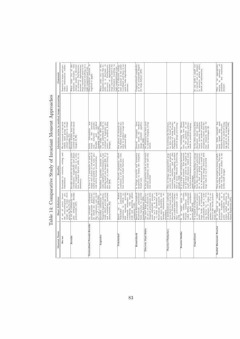
Tab
le14:Com
parativeStudyof
Invarian
tMom
entApproaches
Mom
ent
Nam
eShort
Definitio
nBenefits
Literature
revie
win
medic
alim
age
processin
gCom
ment
Hu
set
Ase
tofseven
invari-
ant
non-o
rthogonal
mo-
ments
up
toord
er
three
given
by
Hu
[74,91]
Invariant
toro
tation,
scaling
and
translation.
Hu
setmomentis
themost
wid
ely
use
dgro
up
of
in-
variantmoments
inim
age
pro
cessin
g[74]
Sensitiveto
noiseand
pro
-vid
es
inform
ation
redun-
dancy.
Zernik
eA
set
of
continuous
com-
plex
orthogonal
Zern
ike
polynomials
[127].
Zern
ikemoments
are
given
inpolar
coord
inate
s;magnitude
and
phase
where
magnitude
valu
eis
aro
ta-
tion
invariant
featu
rewith
no
re-
dundancy.
Severa
lstudies
have
been
carried
outon
blood
smear
images[9,39].
When
ord
er
(m)
of
the
moments
incre
ase
s,th
ischange
makes
adecre
ase
inaccura
cy.
Furtherm
ore
,because
of
digitalization,
larg
evariationsneed
tobe
transform
ed
resu
ltin
gin
ahigh
computa
tionalcost.
Generalized
Pseudo-Z
ernik
eAn
exte
nded
orthogonal
pse
udo-zern
ike
polynomi-
als
which
are
defined
on
the
continuous
unit
circle
(x2+y2
=1)[249,250].
Afreeα
≥1
para
mete
ris
use
dto
adju
stzero
points
ofre
al-valu
ed
of
radialpolynomialto
,in
turn
,pro
-vid
ebetterfeatu
repre
senta
tion.
Little
inform
ation
was
found
on
the
associa-
tion
betw
een
pse
udo-
Zern
ike
and
medical
imagin
g[180,181,182].
Discre
tization
pro
cess
isre
quired
toapply.
Legendre
Exte
nded
continuous
or-
thogonalLegendre
polyno-
mials
which
pro
vid
esc
ale
and
translation
invariant
chara
cte
ristic
[62].
Modifi
ed
Legendre
moment
pro
-vid
essignifi
cantperform
ancein
an-
alyzin
gsm
all
sizeim
ages[62].
Itis
also
robust
tonoise
and
blu
rry
ef-
fect[264]
The
study
in2011
[229]
isonly
publish
ed
work
toevalu
ate
of
Legendre
mo-
ments
on
medical
X-R
ay
Images.
When
ord
er
( m)
of
the
moments
incre
ase
sth
isre
-su
lts
ina
decre
ase
inaccura
cy.
Furtherm
ore
,because
of
digitalization
larg
evariationsneed
tobe
transform
ed,
resu
ltin
gin
high
computa
tionalcost.
Tchebichef
Base
don
aRadial
Tchebichef
polynomial
expansion
inwhich
ra-
dial
moments
pro
vid
ero
tational
invariance
by
considering
only
magni-
tude
and
ignoring
phase
component[149].
Itis
adiscre
teexpansion,
which
constru
cts
ase
tofsc
ale
and
rota
-tion
invariantro
bust
featu
res.
Few
pieces
ofre
search
us-
ing
RadialTchebichefmo-
mentin
medicalim
ageare
addre
ssed
[92].
Itis
as
adiscre
teorthog-
onalmoment
inth
epolar
coord
inate
and
there
isno
need
tota
ke
digitalization
pro
cess.
Krawtchouk
Base
dondiscre
teweighte
dKra
wtchouk
polynomials
basis
function
topro
vid
einvariantfeatu
res[256].
Itbrings
recursive
and
symmetry
pro
perties
tolessen
the
computa
-tionalcost.
Severa
lattempts
have
been
made
for
medical
image
analysis
applica-
tions[248].
Computa
tionalcomplexity
isatan
accepta
ble
degre
eforlarg
edata
set[256].
Discrete
DualH
ahn
The
dualHahn
polynomi-
als
are
ase
tofdiscre
teor-
thogonalpolynomials
with
more
adju
stable
para
me-
ters
(α1
≥0,α
2>
−1)
than
Tchebichef
and
Kra
wtchouk
moments
togive
more
flexib
ility
with
min
imal
inform
ation
re-
dundancy.
Ithaspro
pertiessu
ch
asre
currence
relation,sy
mmetry,sc
ale
and
rota
-tion
invariant
Noattentionhasbeenpaid
tomedicalim
agin
gre
cog-
nition.
Fourie
r-C
hebyshev
Amath
ematicalcombin
ed
term
which
isbase
don
the
discre
teFourier
transform
andara
dialsh
ifte
dCheby-
shev
polynomials
(ψpq)
[172]
This
setbringsappro
priativepro
p-
erties
such
as
symmetry
pro
perty,
recurrence
relation,
and
italso
takes
adiff
ere
nt
sampling
meth
od
thatis
more
effi
cientin
pre
serv
ing
deta
ils.
[124].
Inre
viewin
gth
elite
ratu
re,
no
data
was
found
on
the
question
ofusing
Fourier-
Chebysh
ev
moment
inmedicalim
agepro
cessin
g.
Fourie
r-M
ellin
Itis
base
dupon
in-
tensity
valu
es,
circular
Fourier
transform
and
radial
Mellin
polynomials
ina
polar
coord
inate
system
[207,212].
Itis
asc
ale
and
rota
tion-invariant
orthogonalmoment.
This
moment
sethasmore
zero
sin
the
region
of
small
radialdista
nce,
which
leads
tobetterperform
ancein
pre
senceof
small
images.
Inre
viewin
gth
elite
ra-
ture
,no
data
was
found
on
the
question
of
us-
ing
Fourier-M
ellin
polyno-
mials
inmedicalim
agin
g.
Gegenbauer
Itis
base
don
Gegenbauer
or
ultra
-spherical
polyno-
mials.
Itre
pre
sents
alarg
ebody
of
orthogonal
polynomials
with
asc
al-
ing
facto
r(α
>−0.5)
adju
stment,
Γre
fers
togamma
function,Pn
re-
late
dto
theJacobipolyno-
mials
[89].
Themost
obviousfindin
gto
emerg
efrom
this
ultra
-sphericalpolynomi-
als
isth
at
aglobal
chara
cte
ris-
tic
isdete
rmin
ed
with
asm
all
(α)
where
as
localim
age
featu
res
with
larg
evalu
eof(α
)is
extracte
d.
Sofar,
there
hasbeenlittle
discussion
about
Gegen-
bauer
moment
implemen-
tation
inmedical
pattern
recognition
term
sand
fur-
ther
rese
arch
should
be
doneto
investigate
[8].
Inour
work
asm
all
(α)
iscarried
out
on
data
set
topre
serv
eglobal
white
blood
cell
inform
ation.
Radia
lH
arm
onic
Fourie
rIt
isbase
don
radial
polynomial
and
discre
teFourier
transform
ina
polar
coord
inate
system,
where
radial
function
isdefined
by
thre
econdi-
tionalEquations[187].
Theyare
invariantin
term
sofsh
ift-
ing,sc
aling,and
rota
tion.This
mo-
ment
set
has
better
ability
tode-
scribesm
all
images
Very
little
rese
arch
has
been
found
that
use
dRadial-Harm
onic-F
ourier
moments
inmedicalim
ag-
ing
and
inth
ere
cognition
ofcell
smearim
ages[186].
This
isan
appro
priate
option
inpre
sence
of
available
low
reso
lution
data
set.
83
Relative shape measurements vector:
In addition, relative area (Ar), is also considered in white blood cells classification in
our study. Shape feature vector includes invariant orthogonal moments and relative
area for each white blood cell image.
As a result, and after relevant and redundant feature analysis (see Section 5.6) this
suggests that moment implementation provides 332−36 = 296 features corresponding
to 11 − 1 = 10 different invariant moment approaches (all approaches listed above
excluding Legendre). In conclusion, the final shape feature vector consists of 297
feature coefficients for each white blood cell sample, composed of (296) invariant
moment coefficients and (1) measure for Ar.
5.3.3 Texture Features
The following features aim to quantify the overall local density variability inside the
object. It is often difficult to visualize textural features and associate feature values
with the appearance of cells.
The vector includes features associated with the Laplace transform, gradient-
based, flat texture features [193], and also co-occurrence matrix [82] which is defined
over a white blood cell image to be the distribution of co-occurring values at a given
offset. Various combinations of the matrix are taken to generate features called Har-
alick features [82] (namely, the angular second moment, contrast, correlation, sum
of squares: variance, inverse difference moment, energy, and entropy). Afterwards,
six parameters approximating visual perception is used based on the Tamura fea-
ture [222]. In addition, run-length is an another texture coarseness measurement at
typical directions such as 0, 45, 90, and 135 degrees [223]. 11 features for a given
gray-level for each individual white blood cell image are extracted. Dual-tree com-
plex wavelet is also examined in this research. It calculates coefficients along rows
and columns, and in six directions and angles at each individual pixel.
The setting, details and proposed framework using these textural features are ad-
dressed as follows. This section creates a high dimensional feature vector . These
features include gradient transformation features (▽f(x, y) = (∂f(x,y)∂x
, ∂f(x,y)∂y
)), lapla-
cian transformation features (▽2f(x, y) = ∂2f(x,y)∂x2 + ∂2f(x,y)
∂y2), flat texture features, and
also co-occurrence matrix [82] which is defined over an white blood cell image to be
the distribution of co-occurring values at a given offset. Let n×m be the size of the
84
input image I. Also, let (△x,△y) be the parameters of an offset. Mathematically, a
primary co-occurrence matrix definition is given by:
C△x,△y(i, j) =n∑
x=1
m∑y=1
{1 ; if I(x, y) = i & I(x+△x, y +△y) = j
0 otherwise.
Each entry is therefore considered to be the probability that a pixel with value i will be
found adjacent to a pixel of value j. It estimates the probability that pixel I(k, l) has
intensity i and a pixel I(m,n) has intensity j. Various combinations of the matrix are
taken to generate features called Haralick features [82] (namely, the angular second
moment, contrast, correlation, sum of squares: variance, inverse difference moment,
energy, and entropy).
Afterwards, six parameters approximating visual perception is used based on the
Tamura feature [222]. Tamura textural features include namely, coarseness (coarse
versus fine), contrast (high versus low), directionality (directional versus non-directional),
linelikeness (line-like versus blob-like), regularity (regular versus irregular), and rough-
ness (rough vs. smooth). In addition, run-length [223] is an another texture coarse-
ness measurement in specified directions. Run is a series of consecutive pixels which
have the same intensity along with a specific direction. The dimension of run-length
matrix is M by N , where M is the number of gray levels and N is the maximum run
length at typical directions such as 0, 45, 90, and 135 degrees [223]. 11 features such
as short run emphasis (SRE), long run emphasis (LRE), gray-level non-uniformity
(GLN), run length non-uniformity (RLN), run percentage (RP), low gray-level run
emphasis (LGRE), high gray-level run emphasis (HGRE), and some other ones are
consequently extracted from run-length matrices R(ı, ȷ). For a given gray-level, in-
dividual white blood cell image, a run-length matrix R(ı, ȷ) quantifies the coarseness
of a white blood cell texture at 0, 45, 90, and 135 degrees defined as the number of
runs with pixels of gray level ı and run length ȷ. Further explanations and medical
imaging application on run-length features are also addressed in various articles such
as [103,188,232].
Initially, in this work gradient and laplacian transformation, flat texture with
r = 0, seven Haralick features, three Tamura features i.e., coarseness, contrast, and
directionality, eleven run length statistics and dual tree complex wavelet transform
in six directions are considered.
85
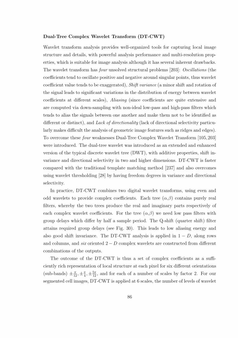
Dual-Tree Complex Wavelet Transform (DT-CWT)
Wavelet transform analysis provides well-organized tools for capturing local image
structure and details, with powerful analysis performance and multi-resolution prop-
erties, which is suitable for image analysis although it has several inherent drawbacks.
The wavelet transform has four unsolved structural problems [203]: Oscillations (the
coefficients tend to oscillate positive and negative around singular points, thus wavelet
coefficient value tends to be exaggerated), Shift variance (a minor shift and rotation of
the signal leads to significant variations in the distribution of energy between wavelet
coefficients at different scales), Aliasing (since coefficients are quite extensive and
are computed via down-sampling with non-ideal low-pass and high-pass filters which
tends to alias the signals between one another and make them not to be identified as
different or distinct), and Lack of directionality (lack of directional selectivity particu-
larly makes difficult the analysis of geometric image features such as ridges and edges).
To overcome these four weaknesses Dual-Tree Complex Wavelet Transform [105,203]
were introduced. The dual-tree wavelet was introduced as an extended and enhanced
version of the typical discrete wavelet tree (DWT), with additive properties, shift in-
variance and directional selectivity in two and higher dimensions. DT-CWT is faster
compared with the traditional template matching method [237] and also overcomes
using wavelet thresholding [28] by having freedom degrees in variance and directional
selectivity.
In practice, DT-CWT combines two digital wavelet transforms, using even and
odd wavelets to provide complex coefficients. Each tree (α,β) contains purely real
filters, whereby the two trees produce the real and imaginary parts respectively of
each complex wavelet coefficients. For the tree (α,β) we need low pass filters with
group delays which differ by half a sample period. The Q-shift (quarter shift) filter
attains required group delays (see Fig. 30). This leads to low aliasing energy and
also good shift invariance. The DT-CWT analysis is applied in 1 − D, along rows
and columns, and six oriented 2−D complex wavelets are constructed from different
combinations of the outputs.
The outcome of the DT-CWT is thus a set of complex coefficients as a suffi-
ciently rich representation of local structure at each pixel for six different orientations
(sub-bands) ± π12,±π
4,±5π
12, and for each of a number of scales by factor 2. For our
segmented cell images, DT-CWT is applied at 6 scales, the number of levels of wavelet
86
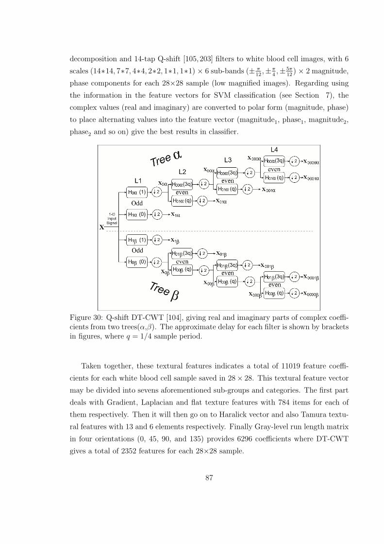
decomposition and 14-tap Q-shift [105,203] filters to white blood cell images, with 6
scales (14∗14, 7∗7, 4∗4, 2∗2, 1∗1, 1∗1) × 6 sub-bands (± π12,±π
4,±5π
12) × 2 magnitude,
phase components for each 28×28 sample (low magnified images). Regarding using
the information in the feature vectors for SVM classification (see Section 7), the
complex values (real and imaginary) are converted to polar form (magnitude, phase)
to place alternating values into the feature vector (magnitude1, phase1, magnitude2,
phase2 and so on) give the best results in classifier.
Figure 30: Q-shift DT-CWT [104], giving real and imaginary parts of complex coeffi-cients from two trees(α,β). The approximate delay for each filter is shown by bracketsin figures, where q = 1/4 sample period.
Taken together, these textural features indicates a total of 11019 feature coeffi-
cients for each white blood cell sample saved in 28× 28. This textural feature vector
may be divided into sevens aforementioned sub-groups and categories. The first part
deals with Gradient, Laplacian and flat texture features with 784 items for each of
them respectively. Then it will then go on to Haralick vector and also Tamura textu-
ral features with 13 and 6 elements respectively. Finally Gray-level run length matrix
in four orientations (0, 45, 90, and 135) provides 6296 coefficients where DT-CWT
gives a total of 2352 features for each 28×28 sample.
87
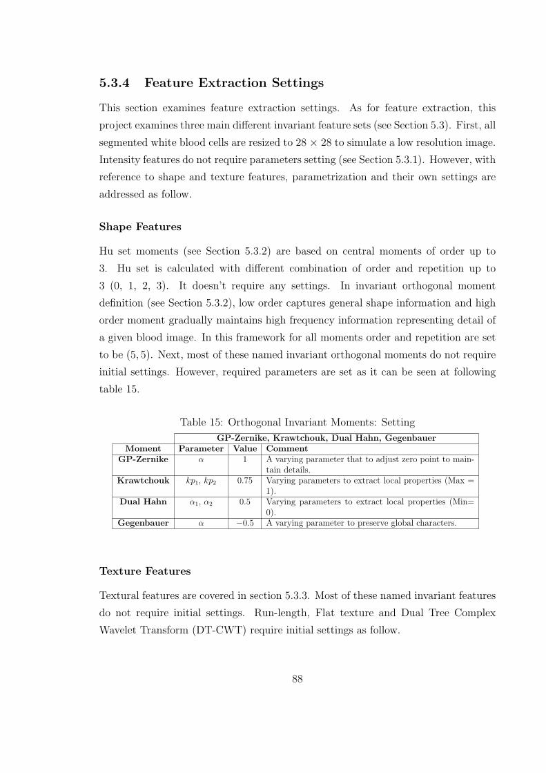
5.3.4 Feature Extraction Settings
This section examines feature extraction settings. As for feature extraction, this
project examines three main different invariant feature sets (see Section 5.3). First, all
segmented white blood cells are resized to 28 × 28 to simulate a low resolution image.
Intensity features do not require parameters setting (see Section 5.3.1). However, with
reference to shape and texture features, parametrization and their own settings are
addressed as follow.
Shape Features
Hu set moments (see Section 5.3.2) are based on central moments of order up to
3. Hu set is calculated with different combination of order and repetition up to
3 (0, 1, 2, 3). It doesn’t require any settings. In invariant orthogonal moment
definition (see Section 5.3.2), low order captures general shape information and high
order moment gradually maintains high frequency information representing detail of
a given blood image. In this framework for all moments order and repetition are set
to be (5, 5). Next, most of these named invariant orthogonal moments do not require
initial settings. However, required parameters are set as it can be seen at following
table 15.
Table 15: Orthogonal Invariant Moments: Setting
GP-Zernike, Krawtchouk, Dual Hahn, GegenbauerMoment Parameter Value Comment
GP-Zernike α 1 A varying parameter that to adjust zero point to main-tain details.
Krawtchouk kp1, kp2 0.75 Varying parameters to extract local properties (Max =1).
Dual Hahn α1, α2 0.5 Varying parameters to extract local properties (Min=0).
Gegenbauer α −0.5 A varying parameter to preserve global characters.
Texture Features
Textural features are covered in section 5.3.3. Most of these named invariant features
do not require initial settings. Run-length, Flat texture and Dual Tree Complex
Wavelet Transform (DT-CWT) require initial settings as follow.
88
Run-length [103,188,232] as a texture coarseness measurement is applied at typical
directions such as 0, 45, 90, and 135 degrees. Next, flat texture [193] is applied with
r = 0 where r is the arbitrary window size of the median filter. Finally, For our
segmented cell images, DT-CWT [105, 203] is applied at 6 scales, the number of
levels of wavelet decomposition and 14-tap Q-shift filters to image samples, and in
6 directions. It also should be noted that wavelet complex coefficients are converted
into magnitude, phase components for each 28×28 sample (low magnified images) to
set in a feature vector.
5.4 Advantages of Features
This section reviews briefly the usefulness of the aforementioned features in white
blood cell classification. Each feature alone has certain important benefits for white
blood cell detection. This study uses a combination of features, selected based on
specific criteria, as depicted in table(see Table 21).
Intensity Histogram Features:
This measure describes globally the color change in a given white blood cell sample.
However, for the purpose of white blood cell detection, such findings are not always
sufficiently reliable to be extrapolated to all datasets. In addition, it was found that,
with low quality, or degraded images, results were not very encouraging (see Tables
24, 23).
Hu set of Invariant Moments:
These coefficients are invariant to shape changes in rotation, scaling and translation.
However, higher-order Hu set moments are sensitive to noise and they also include
redundant information.
Orthogonal Invariant Moment:
They are invariant in rotation, scaling and translation and they provide minimal infor-
mation redundancy. Some of these, like Dual Hahn, Fourier-Mellin, Radial Harmonic
89
Fourier and Fourier Chebyshev are adequate for extraction of local details with their
own varying parameters (see Tables 14, 21).
Haralick Features:
It is based on a probability that a given pixel a has value of i while simultaneously
an adjacent pixel b has value of j. Thirteen features were extracted by Haralick
from the Gray-Level Co-Occurrence Matrix (GLCM). This provides a general view
of the distribution of co-occurring values in a given white blood cell. It represents a
statistical approach, which characterizes the amount of spread with regard to intensity
values in adjacent pixels. The colour feature alone is not enough to interpret a
small white blood cell image. However, the combination described provides a global
attribute with local information.
Dual Tree Complex Wavelet Transform:
It provides a local, invariant rich characterization, by using a dual tree of wavelet
filters along the rows and columns, and in six directions and angles at each individual
pixel. It brings non-redundant information, and it also overcomes the four major
weaknesses typical of Wavelet Transform.
Gray Level Run Length:
It is a coarseness measurement. Run detects a series of consecutive pixels which have
the same intensity along the typical directions such as 0, 45, 90, and 135 degrees.
Intensity histogram lacks detailed information. However, Run is a measure that can
be used to distinguish images with different local appearances, even though they have
similar histograms. It can efficiently describe the colors, directions and geometrical
shapes of the white blood cells in an image. Eleven features were extracted by Run
calculation.
Tamura Features:
It is a series of features that correspond to human visual perception. This is the great
advantage of the Tamura features. Six features were extracted by Tamura concept. It
90
should be noted that the first three features: coarseness, contrast, and directionality,
which depict a white blood cell sample in accordance with visual perception, are
particularly important.
Gradient Feature:
It is a measure to describe the directional change of gray intensity values in a given
white blood cell image. Gradient feature is robust to lighting and camera changes. It
is a characteristic appropriate for WBC detection, of which this work takes advantage.
Laplacian Feature:
The Laplace transformation is a means to establish borders and boundaries of white
blood cells, via zero sum of the second partial derivatives. Essentially, this feature
examines the velocity of gradient changes in a given white blood cell, since a white
blood cell lacks strong edges and boundaries. Thus, a link between these features and
white blood cell detection is weak.
Flat Texture:
It represents the smoothing difference between the original white blood cell and a
median filtered image. The average value of a flat texture image describes the unbal-
ance in light and dark pixel distributions. The degree of smoothness is calculated by
varying the arbitrary parameter (r) as a multiple of the median calculated.
5.5 Comparison of the Proposed Approach to State-
of-the-Art
This section focuses on comparative studies on state-of-the-art feature extraction and
white blood cell detection. Authors in [160] used a feature set composed of shape
and color texture based features. The feature set are area of cell and nucleus, ratio
of nucleus area and perimeter length over cell, compactness and boundary, energy of
nucleus, and also from second and third-order central moments. As mentioned before,
varying capturing angles and different magnification cause non reliable variant cell
91
appearance in correspondence with area, perimeters and roundness or other similar
measures like these. Also, second and third-order central moments as Hu set mo-
ments are also so sensitive to noise and it is with redundant information. Thus their
performance depends on their own dataset and the generalizability of this published
research is problematic.
Authors in [34] used chromatic feature sets that are very questionable in different
conditions (see Table 24). Authors in [213] examined shape features such as eccen-
tricity of the nucleus and cytoplasm contours, compactness of the nucleus, area-ratio
and the number of nucleus lobes. This article also used texture features such as gray-
level co-occurrence matrix(GLCM) and auto-correlation matrix to detect cells. The
key problem with this explanation is that separation nucleus and cytoplasm in low
resolution images is not easy as well as cytoplasm contours and number of nucleus
lobes is very problematic in different possible adverse conditions. However, gray-level
co-occurrence matrix(GLCM) provides several invariant statistics about the texture
of a white blood cell image that it brings appropriate characteristics even in low
resolution images (see Section. 5.3.3).
Authors in [183] used a 18 color, 8 shape dimensional feature vector and sup-
port vector machine (SVM). With reference to color characteristic, authors used
mean, standard deviation, and skewness calculation separately for hue, saturation,
and luminance. Furthermore, authors examined contour-based descriptors such as
convexity, perimeter, principal axis ratio, compactness, circular and elliptic variance.
All these contour-based descriptors reviewed so far cannot represent ideally white
blood cell shapes for which the complete and continuous boundary information is not
ideally available with granular and non-uniform borders. However, mean, standard
deviation, and skewness gives appropriate characteristic even in low quality image.
Authors in [228] used four white blood cell nucleus features. These features are
first and second Granulometric moments [200], area of the nucleus and the location of
its pattern spectrum’s peak. It is found that all these four shape features applied on
segmented nucleus where this segmentation is not very easy in all possible low quality
images. In addition, to obtain granulometric moments different structure elements
should be used to analyze morphological characteristics of white blood cell nucleus
where these settings are not reliable in presence of irregular messy nucleus shapes.
Furthermore, granulometric operation is sensitive to noise and false calculation will
92
be addressed in moment results.
Authors in [106] used 12 ensemble features such as shape, intensity, and texture
features with 71 dimensions. These features as shape descriptors are; area, perimeter,
eccentricity, first and second invariant moment, the number of nuclei. For the intensity
feature; average and standard deviation of each nucleus and lastly, for the texture
feature, 59 LBPs (local binary patterns) are used. This argument relies too heavily
on qualitative analysis of blood slides and the existing accounts fail to resolve cell
discrimination with different quality.
Authors in [189] used feature vector which was made of nucleus and cytoplasm
area, nucleus perimeter, number of separated parts of nucleus, mean, variance of nu-
cleus and cytoplasm boundaries, co-occurrence matrix and also local binary patterns
(LBP) measures. In a broadly speaking, questions have been raised about the nucleus
and cytoplasm area, nucleus perimeter, number of separated parts of nucleus and cy-
toplasm boundaries. However, co-occurrence matrix and also local binary patterns
(LBP) measures are appropriate candidates in different dataset.
Authors in [38] proposed a white blood cell classification with 19 features evaluated
for the nucleus and cytoplasm. These features are such as area, perimeter, convex
area, solidity, orientation, eccentricity, circularity, ratio of nucleus area to area of white
blood cell, entropy of the cytoplasm, and mean gray-level intensity of the cytoplasm.
Almost the same feature extraction strategy is addressed in other work [51] with
reference to geometrical shape features such as area, solidity, eccentricity, the area of
convex part of the nucleus and perimeter. As a result, in a low quality image using
these named shape features is questionable and the generalizability of only these
features on this issue is problematic.
Overall, the difficulties in detection and classification are further aggravated by
the fact that there is no definitive procedure exactly prescribing what features should
be generated, or what features should be used in each specific case. Previous work
as mentioned in detail used features that they are not always invariant and can be
changed in different conditions and resolutions. Shape features such as area, perimeter
and so on rely heavily on their own data set and of course these findings cannot be
extrapolated to all possible dataset. Previous researches did not investigate benefits
of local data preserving techniques such as dual-tree complex wavelet transform, Run
length and invariant orthogonal moments such as Fourier-Mellin, Radial Harmonic
93
Fourier, Dual Hahn.
In reality, this work suggests some proper invariant features that maintain local
information even in presence of low quality images where internal details are not
easy to distinguish. These features can be named as orthogonal invariant moments
(i.e, Radial Harmonic Fourier, Dual Hahn, Fourier- Mellin), DT-CWT (Dual-Tree
Complex Wavelet Transform), run length and Tamura features. Experimental results
prove that these named invariant features bring benefits in presence of low quality
imaged.
5.6 Relevant and Redundant Features
In this section we obtain a set of relevant and least redundant features among all can-
didates. Intensity (see Section. 5.3.1) and texture features (see Section. 5.3.3) are not
correlated and thus they have negligible redundancy and large relevance. However,
shape features are based on invariant moment descriptors (see sub-section 5.3.2) in
which similar characteristics can be found to some extent (see Table 14). The eval-
uation procedure for shape features has been organised as follows. The first part
deals with distribution functions. In both Kolmogorov - Smirnov and Wilcoxon-
Mann-Whitney tests, all scaled feature data with primary matrix (140 rows = 28
samples per each five class) are used to evaluate distribution behaviour. In the next
step, Pearson and Spearman measure objectively linear correlation or/and monotonic
function behaviour while Kendall addresses the rankings of the correlation coefficients
for input data.
5.6.1 Kolmogorov - Smirnov (K-S)
Kolmogorov - Smirnov method provides a non-parametric measure test to determine
whether an empirical density function over available dataset can be mapped to a
particular known distribution model to describe the statistical properties of feature
vector [170]. It calculates the vertical distance (KSD) between the cumulative distri-
bution function (CDF ) of the reference hypothetical distribution and the empirical
distribution function EDF . Two sided (K-S) test is used to compare two sample sets
(two invariant moments in this case) without any particular distribution assumptions.
The (KSD) is defined by following equation:
94
KSD = supn |CDF (x)− EDF (x)n|
The null hypothesis, meaning that two distributions are similar is accepted when
KSD is less than the 5% significance level.
Dataset and K-S interpreting: For all samples, the aforementioned shape feature
vector (see sub-section 5.3.2), the two-sided K-S test is used to calculate the sig-
nificance value of vertical distances (KSD) for all available pairs of feature moment
candidates. The values obtained by applying the null hypothesis tell us whether two
mutually independent feature sets are sufficiently close to each other to belong to the
same distribution. The experimental results are summarized in table 16.
The table 16 presents p-values obtained from the preliminary analysis of two
sided Kolmogorov-Smirnov test to evaluate distribution similarity among 11 invariant
moments. It can be seen from the data in table that all these moments are drawn from
the same distribution (null hypothesis is accepted). This tendency is also reflected
in the p-value. From this data, we can see that the lowest discriminatory power
is 0.42491, which occurs between Legendre and Gegenbauer moments. In contrast,
there is a clear trend of increasing p-values, 0.9762 between Krawtchouk and Legendre
moments and, 0.9906 between Radial Tchebichef and Zernike moments.
To make a firm determination, Mann-Whitney test is also used here (see. 5.6.2).
Both the Mann-Whitney and the Kolmogorov-Smirnov tests are non-parametric tests
to compare two groups of invariant moment data, and both methods calculate p-values
over the same null hypothesis but using different approach.
K-S test computes p-values after cumulative distribution comparison of the two
data moment sets and WMW test then computes p-values that depend on the dis-
crepancy between the mean ranks of the two moments after ranking all the moment
coefficient values from low to high. The K-S test is more sensitive to differences be-
tween any two feature moments, which are reflected in small p-values. In contrast,
the WMW test is mainly sensitive to changes in median value. The WMW test has
inherent and structural ability to handle tied values, whereas K-S test does not work
very well with ties. In presence of moment categories, many ties are possible. For
this reason, it is highly recommended to perform the WMW test,in addition to K-S
test.
95
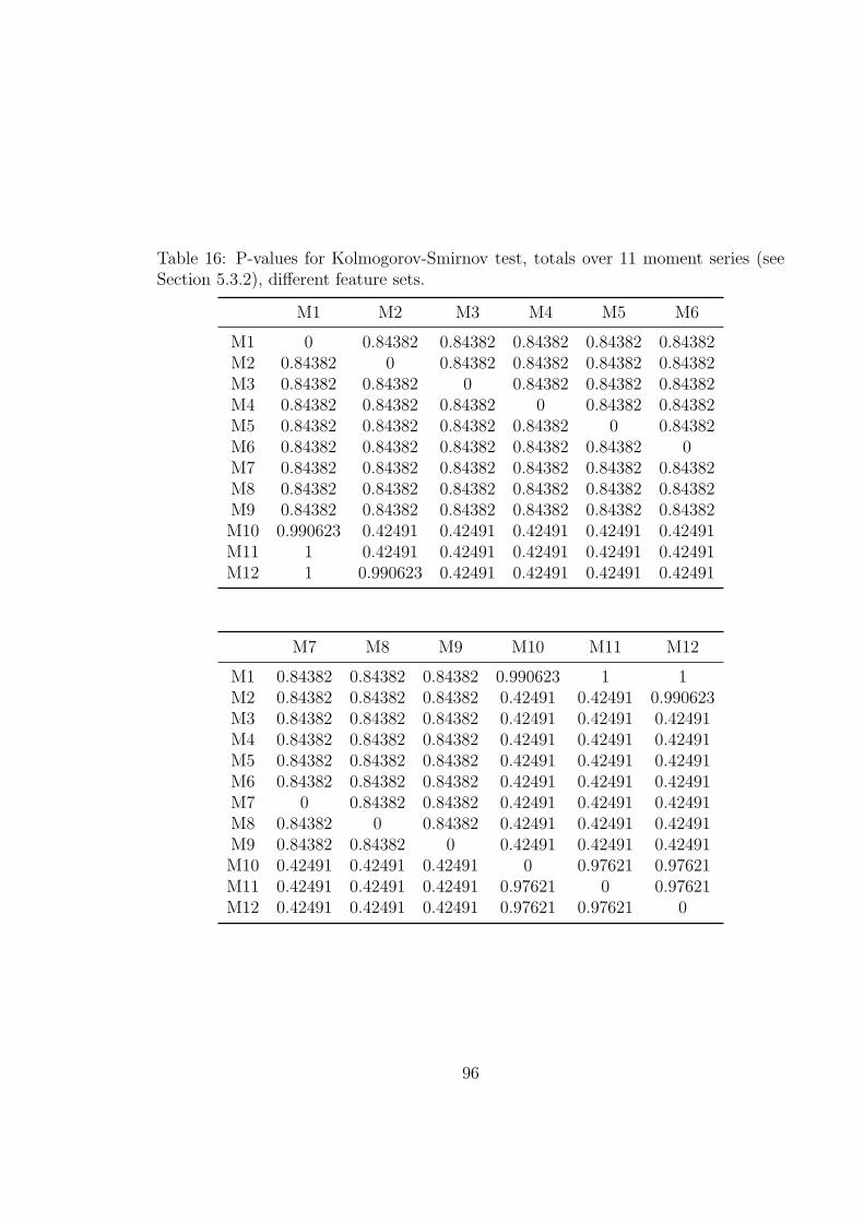
Table 16: P-values for Kolmogorov-Smirnov test, totals over 11 moment series (seeSection 5.3.2), different feature sets.
M1 M2 M3 M4 M5 M6
M1 0 0.84382 0.84382 0.84382 0.84382 0.84382M2 0.84382 0 0.84382 0.84382 0.84382 0.84382M3 0.84382 0.84382 0 0.84382 0.84382 0.84382M4 0.84382 0.84382 0.84382 0 0.84382 0.84382M5 0.84382 0.84382 0.84382 0.84382 0 0.84382M6 0.84382 0.84382 0.84382 0.84382 0.84382 0M7 0.84382 0.84382 0.84382 0.84382 0.84382 0.84382M8 0.84382 0.84382 0.84382 0.84382 0.84382 0.84382M9 0.84382 0.84382 0.84382 0.84382 0.84382 0.84382M10 0.990623 0.42491 0.42491 0.42491 0.42491 0.42491M11 1 0.42491 0.42491 0.42491 0.42491 0.42491M12 1 0.990623 0.42491 0.42491 0.42491 0.42491
M7 M8 M9 M10 M11 M12
M1 0.84382 0.84382 0.84382 0.990623 1 1M2 0.84382 0.84382 0.84382 0.42491 0.42491 0.990623M3 0.84382 0.84382 0.84382 0.42491 0.42491 0.42491M4 0.84382 0.84382 0.84382 0.42491 0.42491 0.42491M5 0.84382 0.84382 0.84382 0.42491 0.42491 0.42491M6 0.84382 0.84382 0.84382 0.42491 0.42491 0.42491M7 0 0.84382 0.84382 0.42491 0.42491 0.42491M8 0.84382 0 0.84382 0.42491 0.42491 0.42491M9 0.84382 0.84382 0 0.42491 0.42491 0.42491M10 0.42491 0.42491 0.42491 0 0.97621 0.97621M11 0.42491 0.42491 0.42491 0.97621 0 0.97621M12 0.42491 0.42491 0.42491 0.97621 0.97621 0
96
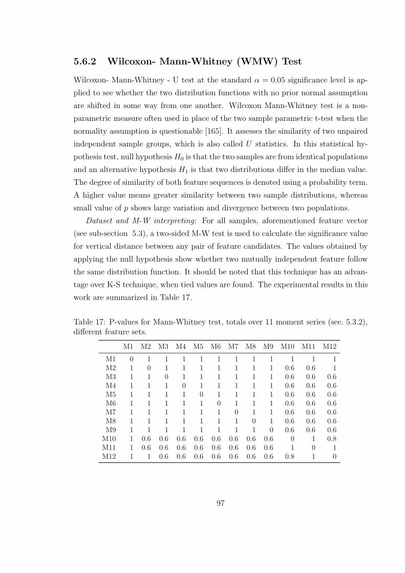
5.6.2 Wilcoxon- Mann-Whitney (WMW) Test
Wilcoxon- Mann-Whitney - U test at the standard α = 0.05 significance level is ap-
plied to see whether the two distribution functions with no prior normal assumption
are shifted in some way from one another. Wilcoxon Mann-Whitney test is a non-
parametric measure often used in place of the two sample parametric t-test when the
normality assumption is questionable [165]. It assesses the similarity of two unpaired
independent sample groups, which is also called U statistics. In this statistical hy-
pothesis test, null hypothesisH0 is that the two samples are from identical populations
and an alternative hypothesis H1 is that two distributions differ in the median value.
The degree of similarity of both feature sequences is denoted using a probability term.
A higher value means greater similarity between two sample distributions, whereas
small value of p shows large variation and divergence between two populations.
Dataset and M-W interpreting: For all samples, aforementioned feature vector
(see sub-section 5.3), a two-sided M-W test is used to calculate the significance value
for vertical distance between any pair of feature candidates. The values obtained by
applying the null hypothesis show whether two mutually independent feature follow
the same distribution function. It should be noted that this technique has an advan-
tage over K-S technique, when tied values are found. The experimental results in this
work are summarized in Table 17.
Table 17: P-values for Mann-Whitney test, totals over 11 moment series (see. 5.3.2),different feature sets.
M1 M2 M3 M4 M5 M6 M7 M8 M9 M10 M11 M12
M1 0 1 1 1 1 1 1 1 1 1 1 1M2 1 0 1 1 1 1 1 1 1 0.6 0.6 1M3 1 1 0 1 1 1 1 1 1 0.6 0.6 0.6M4 1 1 1 0 1 1 1 1 1 0.6 0.6 0.6M5 1 1 1 1 0 1 1 1 1 0.6 0.6 0.6M6 1 1 1 1 1 0 1 1 1 0.6 0.6 0.6M7 1 1 1 1 1 1 0 1 1 0.6 0.6 0.6M8 1 1 1 1 1 1 1 0 1 0.6 0.6 0.6M9 1 1 1 1 1 1 1 1 0 0.6 0.6 0.6M10 1 0.6 0.6 0.6 0.6 0.6 0.6 0.6 0.6 0 1 0.8M11 1 0.6 0.6 0.6 0.6 0.6 0.6 0.6 0.6 1 0 1M12 1 1 0.6 0.6 0.6 0.6 0.6 0.6 0.6 0.8 1 0
97
As shown in Mann-Whitney test table . 17 there is a significant distribution sim-
ilarity between the aforementioned moment groups. The calculation indicates that
lowest discriminatory power is 0.6 which occurs among Legendre, Krawtchouk and
Radial Tchebichef, whereas p-values are high (0.8 and 1.00) for most other moment
pairs.
So far, it has conclusively been shown that named invariant moment features are
from similar distribution, and it has been demonstrated that a high similarity among
probability distributions exists. A question then arises whether these 11 invariant mo-
ments are redundant, related or totally independent. To address this question, meth-
ods such as Kruskal-Wallis H-Test, Pearson correlation analysis (PCA) and Spearman
Correlation Analysis (SCA) are available to analyse the correlation relationships be-
tween feature variables, and they have been applied as follows.
5.6.3 Kruskal-Wallis H-Test
The one-way analysis of variance (abbreviated one-way ANOVA) is a statistical mea-
sure to examine whether three or more independent input variables are significantly
different. Kruskal-Wallis H- test evaluates the behaviour of these unrelated groups
using variance parameter. In typical one-way ANOVA the assumptions are based on
approximately normally distributed variables and an equal interval scale randomly
drawn from the population, and inputs are normal random variables.
If one or more of the mentioned assumptions are violated, then the one-way
ANOVA may be inaccurate. To overcome this limitation Kruskal Wallis [165, 245]
performs one-way analysis of variance (abbreviated one-way ANOVA) without nor-
mal distribution assumption, by ranking 11 independent moment groups of possibly
unequal sizes (see Section 5.3.2). However, one of the limitations of Kruskal Wallis
(k) explanation is that it does not address where the dissimilarities take place or how
many differences really occur in a completely randomized design.
The returned p value (= 0.0669) from the preliminary analysis of Kruskal Wallis
test indicates a slight correlation between 11 different moments. However, a clear
degree of similarities or differences between groups of moments could not be identified
by this analysis. Further studies, which take the degree of correlation into account
need to be undertaken.
98
5.6.4 Sensitivity Correlation Analysis
Pearson’s correlation: The degree of scatter among feature variables can be evaluated
using Pearson’s correlation measure. It is a measure to evaluate the linear correla-
tion (dependence) between two input feature variables. Pearson statistical approach
computes moment correlation coefficient between two variables x1 and x2. It consid-
ers the strength of a linear relationship between paired input moment feature data.
It is defined as the covariance of the two variables divided by the product of their
standard deviations, which gives values between +1 and −1, where +1 means totally
correlated inputs, 0 means no correlation, and −1 means negative correlation between
two inputs.
The experimental result is summarized in table. 18. As shown in table 18, there
is a significant linear similarity between some of the mentioned moment groups. The
calculation indicates that the highest correlation is between the Radial Tchebichef and
Legendre, and between Gegenbauer and Legendre moments with correlation rates of
0.99 and 0.95 respectively. In contrast, the lowest correlations values are between
Gegenbauer and Radial Harmonic Fourier, and between Fourier-Chebyshev and dual
Hahn moments (0.17 and 0.19 respectively).
Spearman’s correlation: is a non-parametric version of correlation that estimates
variables dependency. It calculates the power of association between two ranked input
feature variables. It is a statistical measure that evaluates how two variables can be
fitted using a monotonic function. A monotonic relationship is an essential primitive
hypothesis of referring the Spearman index correlation. A linear relationship is a firm
underlying assumption that has to be met by Pearson correlation measure. The value
of Spearman’s index ranges between +1 for a perfect monotonic function to −1 which
is furtherest from a mapped monotonic function.
As shown in Spearman test table. 19 there is a significant monotonic relation-
ships among few of the aforementioned moment groups. The calculation indicates
that highest dependency exists between Legendre and Gegenbauer moments, Radial
Tchebichef and Legendre moments, and Krawtchouk and Dual Hahn moments with
correlation rates of 0.9819, 0.9027 and 0.8355 respectively. In contrast, lowest corre-
lations are between Dual Hahn and Gegenbauer, Dual Hahn and Legendre, and Dual
Hahn and Generalized Pseudo-Zernike moments with minimum correlations values of
−0.1335,−0.1104 and 0.0005 respectively.
99
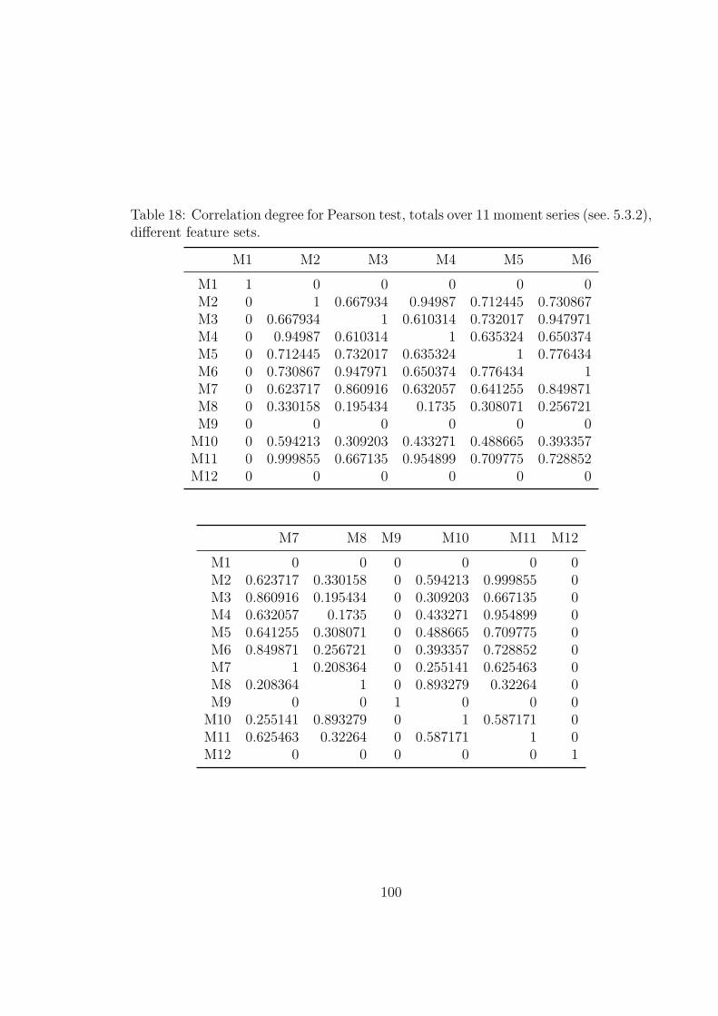
Table 18: Correlation degree for Pearson test, totals over 11 moment series (see. 5.3.2),different feature sets.
M1 M2 M3 M4 M5 M6
M1 1 0 0 0 0 0M2 0 1 0.667934 0.94987 0.712445 0.730867M3 0 0.667934 1 0.610314 0.732017 0.947971M4 0 0.94987 0.610314 1 0.635324 0.650374M5 0 0.712445 0.732017 0.635324 1 0.776434M6 0 0.730867 0.947971 0.650374 0.776434 1M7 0 0.623717 0.860916 0.632057 0.641255 0.849871M8 0 0.330158 0.195434 0.1735 0.308071 0.256721M9 0 0 0 0 0 0M10 0 0.594213 0.309203 0.433271 0.488665 0.393357M11 0 0.999855 0.667135 0.954899 0.709775 0.728852M12 0 0 0 0 0 0
M7 M8 M9 M10 M11 M12
M1 0 0 0 0 0 0M2 0.623717 0.330158 0 0.594213 0.999855 0M3 0.860916 0.195434 0 0.309203 0.667135 0M4 0.632057 0.1735 0 0.433271 0.954899 0M5 0.641255 0.308071 0 0.488665 0.709775 0M6 0.849871 0.256721 0 0.393357 0.728852 0M7 1 0.208364 0 0.255141 0.625463 0M8 0.208364 1 0 0.893279 0.32264 0M9 0 0 1 0 0 0M10 0.255141 0.893279 0 1 0.587171 0M11 0.625463 0.32264 0 0.587171 1 0M12 0 0 0 0 0 1
100
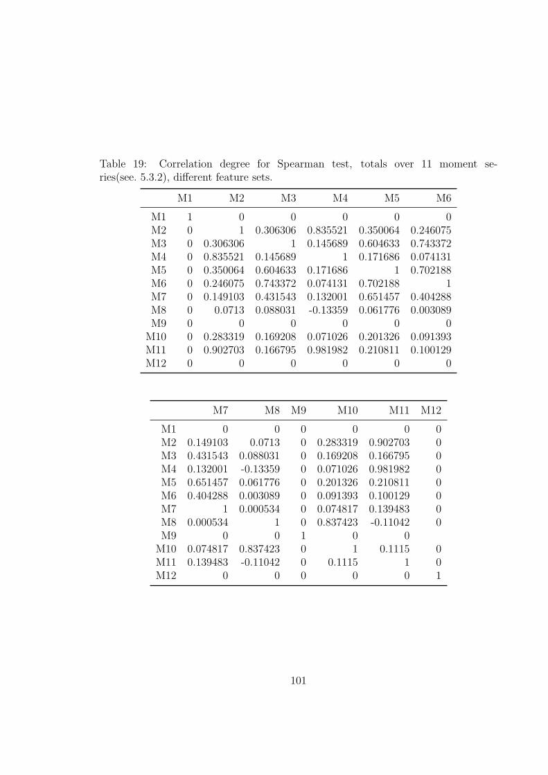
Table 19: Correlation degree for Spearman test, totals over 11 moment se-ries(see. 5.3.2), different feature sets.
M1 M2 M3 M4 M5 M6
M1 1 0 0 0 0 0M2 0 1 0.306306 0.835521 0.350064 0.246075M3 0 0.306306 1 0.145689 0.604633 0.743372M4 0 0.835521 0.145689 1 0.171686 0.074131M5 0 0.350064 0.604633 0.171686 1 0.702188M6 0 0.246075 0.743372 0.074131 0.702188 1M7 0 0.149103 0.431543 0.132001 0.651457 0.404288M8 0 0.0713 0.088031 -0.13359 0.061776 0.003089M9 0 0 0 0 0 0M10 0 0.283319 0.169208 0.071026 0.201326 0.091393M11 0 0.902703 0.166795 0.981982 0.210811 0.100129M12 0 0 0 0 0 0
M7 M8 M9 M10 M11 M12
M1 0 0 0 0 0 0M2 0.149103 0.0713 0 0.283319 0.902703 0M3 0.431543 0.088031 0 0.169208 0.166795 0M4 0.132001 -0.13359 0 0.071026 0.981982 0M5 0.651457 0.061776 0 0.201326 0.210811 0M6 0.404288 0.003089 0 0.091393 0.100129 0M7 1 0.000534 0 0.074817 0.139483 0M8 0.000534 1 0 0.837423 -0.11042 0M9 0 0 1 0 0M10 0.074817 0.837423 0 1 0.1115 0M11 0.139483 -0.11042 0 0.1115 1 0M12 0 0 0 0 0 1
101
After investigation using the three named methods (Kruskal-Wallis H-Test, Spear-
man and Pearson) a very slight evidence of correlation among all the aforesaid invari-
ant moments is found when Kruskal Wallis test is applied. Then, it can be seen from
the data in tables. 18 and 19 that there are significant correlations between Legendre
and Gegenbauer and between Legendre and Radial Tchebichef. In contrast, a decreas-
ing monotonic trend and very low correlations between Dual Hahn and generalized
pseudo-Zernike moments are found.
As a result, the experimental results do not show any significant increase in re-
dundancy among the aforementioned moments. In this evaluation process, Legendre
was found to provide information redundant to Gegenbauer and Radial Tchebichef
to some extent. This suggests that Legendre may be removed from the moment list,
since, according to table 14, both Gegenbauer and Radial Tchebichef moments are
superior to Legendre moment in connection with feature extraction.
Thus, the findings would have been more original and convincing if the orthogonal
Legendre moments had been excluded from the above moment list of the feature vector
(see Section 5.3.2).
5.7 Feature Extraction Contributions
Another contribution is the procedure developed for obtaining optimum invariant
feature set from a comprehensive literature review in mathematical concepts. The
current findings add substantially to our understanding of invariant global features
in preserving details even in presence of low degraded images. For this, an image,
segmented white blood cell, is characterized based on the information such of dual
tree complex wavelet transform, invariant orthogonal moments, Run length, and so
on. This is an approach to address global invariant characteristics and the results are
encouraging.
Feature Extraction
Overall, the difficulties in detection and classification are further aggravated by the
fact that there is no definitive procedure exactly prescribing what features should
be generated, or what features should be used in each specific case. Previous work
as mentioned in detail used features that they are not always invariant and can be
102

changed in different conditions and resolutions. Shape features such as area, perimeter
and so on rely heavily on their own data set and of course these findings cannot be
extrapolated to all possible dataset. Previous researches did not investigate benefits
of local data preserving techniques such as dual-tree complex wavelet transform, Run
length and invariant orthogonal moments such as Fourier-Mellin, Radial Harmonic
Fourier, Dual Hahn. Comparative study and discussion is also found in section 5.5.
103
Chapter 6
Feature Selection
The purpose of feature selection is to provide a smaller effective feature vector com-
pared to the starting data pool. The main objective is to find a way to identify the
features that are worth extracting for optimal accuracy and speed of operation. Fea-
ture selection is to trim a large number of input variables from a given data-set, based
on similarities and discrepancies. Then eventually, the low sensitivity and low cor-
relation between feature and desired classes means weak interaction between feature
and desired output and can be neglected. Feature discriminatory power is a criteria
for feature selection.
6.1 High Dimensional Model Representation
We look at the effect and contribution of multiple features (see Section. 5.3) on the su-
pervised white blood cell classification. Several studies investigating high-dimensional
model representation (HDMR) have been carried out on input and output relationship
analysis. In general, in the field of image processing and feature selection, HDMR has
not yet been investigated comprehensively. To overcome this gap, this work focuses
on the use of HDMR for image processing pattern recognition applications.
In reviewing the literature, several methods with various expansions of high di-
mensional model representations are found, such as factorized high dimensional model
representation (FHDMR) [4, 234], Cut-HDMR [4, 147], (ANOVA)-HDMR [4] as the
analysis of variance (ANOVA) decomposition, random sample(RS)-HDMR [4, 267],
multiple sub-domain random sampling HDMR [260], logarithmic HDMR [233] and
104
hybrid function [235].
HDMR is an appropriate statistical approach to evaluate the input - output map-
ping of a manifold model with many input parameters and using high dimensional
interpolation [4]. High dimensional model representation (HDMR)can therefore eval-
uate the individual or cooperative contributions of the previously defined features
used for classification of white blood cell. Next, the degree of importance and inter-
action of input feature parameters (12104) with regard to white blood cell classes are
determined using sobol global sensitivity analysis.
Before a detailed description of the sensitivity analysis, we will provide a few
definitions related to HDMR. The HDMR output function f(x) utilizes a linear sum
of super - positions of low - dimensional functions, where a multivariate data is given
for a multivariate function f(x) = f(x1, ..., xn) in Rn domain. These sub-divided
terms are set of constant, univariate, bivariate and the other high-variate terms.
f (x) = f0 +n∑
i=1
fi (xi) +n∑
1≤i<j≤n
fij (xi, xj)+
n∑1≤i<j<k≤n
fijk (xi, xj, xk) + · · ·+ f12...n (x1, x2, . . . , xn)
where f0 is the constant mean effect, fi(xi) is the effect of variable xi (each in-
dividual feature coefficient) independently upon the output f(x) (five primary cell
classes). Further, the function fij(xi, xj) is a second order term describing the inter-
action between two feature series (xi and xj) upon the output f(x). It is apparent
that if there is no interaction between the input feature variables, then higher or-
der terms will be zero, where only f0 order and fi(xi) will be written in the HDMR
expansion.
From the experimental results for many input-output systems, it can be seen
that a HDMR expansion up to second order fij(xi, xj) is sufficient to approximate
f(x) in which higher order feature correlations are weak and negligible [126]. In this
work, RS-HDMR approach with a random sample input over the entire domain is
used [4, 267]. The sums of RS-HDMR expansion can be rewritten in the following
form where determination of expansion components is based on shifted Legendre
polynomials approximation and Monte Carlo integration [126]. Input variables are
scaled between 0 and 1 (0 ≤ xinput ≤ 1) [178,267] to create scale - consistent coefficient
105
values.
f (x) = f0 +n∑
i=1
k1∑r=1
αirφr(xi) +
n∑1≤i<j≤n
k2∑p=1
k3∑q=1
βijpqφpq(xi, xj).
Where k1, k2 and k3 are the order of the shifted Legendre polynomials expan-
sion. αir and βij
pq are constant coefficients which are determined using Monte Carlo
integration. Also, φr(xi), φpq(xi, xj) are the shifted Legendre polynomials basis func-
tions. To understand expansion calculation, let’s first define second-order Legendre’s
differential equation:
(1− x2
) d2ydx2
− 2xdy
dx+ n (n+ 1) y = 0
The solution, Legendre polynomial is denoted by Pn(x) which includes order n as
an integer, which provides either odd or even components that are either symmetric
or asymmetric polynomials (Pn (−x) = (−1)nPn (x)). To calculate shifted Legen-
dre polynomials where x 7→ 2x − 1; (Pn (x) = Pn (2x− 1)), calculations are given
by recurrence relation, based on Bonnet’s recursion formula. Therefore, an explicit
representation is obtained:
Pn (x) = (−1)nn∑
c=0
(n
c
)(n+ c
c
)× (−x)c.
Consequently, shifted Legendre polynomial are given in table 20.
Table 20: The first five shifted Legendre polynomial terms
n Pn (x)
0 P0 (x) = 1
1 P1 (x) = 2x− 1
2 P2 (x) = 6x2 − 6x+ 1
3 P3 (x) = 20x3 − 30x2 + 12x− 1
4 P4 (x) = 70x4 − 140x3 + 90x2 − 20x
5 P5 (x) = 252x5 − 630x4 + 560x3 − 210x2 + 30x− 1
Legendre polynomials have the property of orthogonality, i.e. their components
are non-overlapping and non-redundant, and therefore their principal sums can be
obtained. ∫ 1
0
pk(x)pl(x)dx =
{1
2n+1k = l
0 k = l
106
The theory of Legendre polynomials is found in book [110] section 5.2. The op-
timal order of shifted Legendre polynomials is used for approximation of the HDMR
expansion component functions.
Global Feature Sensitivity: The aim of this section is to measure the level of
influence (global sensitivity) of the input feature variable on the white blood cell clas-
sification using RS-HDMR implementation to identify the best feature set. Following
that, the influence of individual each input feature variable is computed using global
sensitivity approach, in which Monte Carlo is the basis function of calculation [214].
An integrable function is defined for an arbitrary monotonic function f(x) that pre-
serves the given order. It is denoted that for every sequence Dn of subsets on [a, b],
we have shown that {µ(Dn)} → 0. Sn is a sample of mentioned partition, which can
be expressed as follows.
{∑(f,Dn, Sn)
}→ K.
An integrable function could be written in the ANOVA - representation form [214]
where total number of sums is 2n. The general definition is
f(x) = f0 +n∑
s=1
n∑i1<...<is
fi1...is(xi1 ,...,xis )
where that the terms are orthogonal and can be expressed as∫ 1
0
fi1...is(xi1 , ..., xis)dxk = 0, k = i1, ..., is.
Above terms can be rewritten in following form :∫f(x)dx = f0∫
f(x)∏k =i
dxk = f0 + fixi∫f(x)
∏k =i,j
dxk = f0 + fixi + fjxj + fijxi,xj .
Global sensitivity is defined by the following equations:
∫f(x)2dx− f 2
0 =n∑
s=1
n∑i1<...<is
∫f 2i1...is(xi1 ,...,xis )dxi1 ,...dxis
.
107
To simply notation, indices D and Di1 , ..., Dis are defined as follows :∫f(x)2dx − f 2
0︸ ︷︷ ︸D
=n∑
s=1
n∑i1<...<is
∫f 2i1...is(xi1 ,...,xis )dxi1 ,...dxis︸ ︷︷ ︸
Di1 ,...,Dis
Therefore, global sensitivity indices are denoted by: Si1,...,is =Di1 ,...,Dis
Dwhere total
of the summation∑n
s=1 si1 +∑n
1<i<j6n Sij, ... + S1,2,...,n = 1. The first order index
Si is the fractional contribution of xi (each individual coefficient) to the variance of
f(x) (five main white blood cell classes), whereas the second order shows the effect of
interaction between xi and xj on the classification outcome. These sensitivity analysis
indices can be continued. Rabitz et al. [4] demonstrated that, often, the low order
interactions of input variables have the dominant impact on the output assignment.
It means that, quite often, the high ranked global sensitivity feature variable input in
mathematical models are first order terms. In the current study, first order Si for all
each individual intensity, shape and texture coefficients are calculated to reach the
most effective feature set.
To date, little evidence has been found associating HDMR with image processing
and pattern recognition. Kaya et al. [101] carried out a number of investigations into
the feature selection by high dimensional model representation, where the experiment
is conducted using a data set which includes 12 band multi spectral images taken over
Tippecanoe County. Article references were searched further for additional relevant
publications, and no other work pertaining to the question of HDMR efficiency in
feature selection for medical images and blood smear slides in particular was found.
A further study with more focus on selecting optimum feature set is suggested in this
work.
6.2 Sequential Feature Selection
Sequential feature selection applies an iterative method and an algorithm that learns
which feature from an initial set, without a transformation, is the most informative at
each step, when choosing the next feature depends on the already selected features.
The method removes unfavourable features but it preserves salient features to reach
the optimum subset combination of features by considering their predictive efficiency
for a given classifier. The method has two distinctive variants. Sequential forward
108
selection (SFS) is a method that keeps adding features, until the criterion function
stops decreasing with new feature candidates. In contrast the process of sequential
backward selection (SBS) starts with a full feature set, and features are removed until
the removal action starts to increase the criterion function [93].
In SFS, new added feature x+ should maximize J(Yk + x+). In an iterative and
incremental procedure, new component is combined with already selected features
(Yk) to increase criterion function (x+ = argx/∈Yk max J(Yk + x+)). Both SFS and
SBS have some drawbacks in practice. Questions have been raised about the update
procedure used in sequential feature selection algorithm. SFS is unable to revise
an already selected a feature vector by removing feature variables after they have
been added. The main limitation of SBS is its inability to improve the efficiency by
restoring a feature variable after it has been abandoned in a previous step. It can
also be seen that without an appropriate criterion to determine a stop point, the SFS
or BSS may run an exhaustive number of combinations(FN
)considering (N) input
samples, which make the process impractical and infeasible because of its complexity.
To improve feature selection sustainability, it is necessary to develop a criterion to
avoid exhaustive comparison. An optimum criterion value means a minimum error
rate in supervised classification where each candidate feature is placed in the new
revised subset vector upon classifier feedback.
Next, 10-fold cross-validation by calling a criterion with different training and
testing subsets of xin and yout is performed. In practice, after computing the mean
criterion values for each candidate feature subset, SFS chooses the optimal feature
candidate that minimizes the mean criterion value. It measures the reduction in
distance between the predicted values and the output testing subset. This process
continues until adding or removing features results in no decrease in criterion.
To date, several studies investigating sequential forward selection (SFS) have been
carried out on medical imaging. Bouatmane et al. [21] used sequential forward se-
lection to assess various sets and to eliminate irrelevant features, in order to classify
prostatic tissue taken from needle biopsies images. Rezatofighi et al. [189] examined
the most discriminative features using sequential forward selection, artificial neural
network (ANN) and support vector machine (SVM) to classify five main types of
white blood cells. Because of a large amount of previous work in SFS, in this work,
SFS approach is applied to a high dimensional feature vector for a comparative study.
109
6.3 Branch and Bound Algorithm
Preliminary work on branch and bound algorithm for selecting the optimal and the
most favourable subset of features in pattern recognition applications was undertaken
by Fukunaga, K (1992) [63]. Branch and bound algorithm relies on procedures that
select a reduced subset of Ds features from a primary larger set of Da inputs, where
a function (J) is used as evaluation criterion. This selects an optimal feature set
without exhaustively exploring the entire search space. It should be noted that,
for any branch & bound algorithm, the (J) function must meet the monotonicity
condition.
J(Xp) ≥ J(Xch); Xch ⊆ Xp.
In brief, branch and bound algorithm assembles a search tree, including end-point
leaves, with target subsets of (Ds) selected features. The start node (root) represents
all initial input features (Da). From this node follows a top-down tree structure,
with branch descendants that are evaluated and updated at nodes, based on criterion
function (J), and the process is called bound algorithm (the best updated evaluation
value). The branches are extended first based on the number of features (Da −Ds)
that should be cut-off. Simultaneously, the bound is updated, as the search tree is
growing and leaf nodes are reached. Afterwards, the sub-tree will be pruned, so that
the associated evaluation value is less or equal to the bound. Search and evaluation
theories typically suffer from certain drawbacks, and this method of analysis has a
number of limitations. Perhaps the most serious disadvantage of this method is that
the computation of criterion value is usually slow.
Different studies have been carried out on investigating branch and bound model,
and modifications have been made to improve the traditional performance.
In reviewing the literature, different methods have been found, including typical
and conventional branch and bound (BB) [63], efficient branch and bound (BB+)
[258], and fast branch and bound (FBB) [216].
Recently in 2013, a globally optimal selection framework has been proposed using
regression [98]. The results, as shown in [98] indicate computational efficiency and
effectiveness of that framework, while shortcomings of existing criterion function (J)
is overcome. In reviewing the literature, Stiglmayr et al. [218] conducted a series of
trials using Branch & Bound methods for medical image registration. Up to date, no
110
work was found in the literature on the question of branch and bound efficiency in
feature selection for medical images, and for blood smear slides in particular. Our
study has the aim of assessing the effectiveness of branch and bound with evaluation
function using regression in feature selection to reach optimal feature subset.
6.4 Experimental Result on Feature Selection
HDMR approach: The initial configuration and setting for this experiment is based
on steps in [267]. All samples (140) are used for the RS-HDMR accuracy test. Also,
the maximum order for approximation of the first order {fi (xi)} terms is 5 where 3
is maximum assigned order for second order {fij (xi, xj)}. Also a ratio control variate
(see Section 2.1 in [267]) to supervise and regulate the Monte Carlo integration error
with 10 iterations is set for the first and second order RS-HDMR component functions.
It also should be noted that in the initial setting to ignore insignificant component
functions from the HDMR expansion where the current white blood cell classification
system has a high number of input features, a threshold mechanism set to 10% (see
Section 2.2 in [267]) is also used.
Global sensitivity analysis for all three feature sets are collected in table 21 where
intensity feature set (see Section 5.3.1) with 788 members composed of 1-784 raw gray
scale intensity value, 785 mean, 786 standard deviation, 787 skewness, and 788 kur-
tosis features and next, shape feature set (see Section 5.3.2) with 297 members com-
posed of 1-7 Hu set, 8 Zernike, 9-44 Hahn, 45-80 generalized pseudo-Zernike, 81-116
Chebyshev, 117-152 Krawtchouk, 153-188 Fourier-Mellin, 189-224 Radial Harmonic
Fourier , 225-260 Fourier-Chebyshev, 261-296 Gegenbauer and 297 for relative area
are considered. Then a texture feature vector with 11019 members (see Section 5.3.3)
composed of 1-784 gradient, 785-1568 Laplacian, 1569-2352 flat texture, 2352-2365
Haralick texture features, 2365-2371 Tamura, 2372-8667 Gray Level Run Length, and
8667-11019 for dual tree complex wavelet transform features is considered. To provide
in-depth analysis of the Sobol index calculation, each of above individual ranges of
features is used separately to estimate global sensitivity values
In this work based on above explanation 273 elements with exact addressed indices
among all 12104 coefficients (almost 2.25%) which are the most convincing set on
HDMR input - output relationship in current white blood cell classification system
111
are selected (HDMRFV ).
In order to compare the performance on classification accuracy using sobol HDMR,
sequential forward selection (SFS) and downwards branch and bound [98] to select
subset with the exact number of (HDMRFV = 273) are also addressed. In connection
with these two approaches, many feature indices should be listed here but an exhaus-
tive review is beyond the scope of this current work. Eventually, to do a comparative
sensitivity analysis, two feature vectors (SFSFV ) and (BBFV ) are created.
Sequential feature selection: Sequential forward selection is initialized using
10-fold cross-validation by repeatedly calling a criterion based support vector machine
setting (see Section 7.2). It is also with different training and testing subsets of χin and
Yout where selected feature are saved into a logical matrix in which row (i) indicates
the features selected at step (i) with minimum criterion value.
Branch and bound: In following subset selection and in order to understand
how branch & bound regulates the best n-variable subset of invariant aforementioned
features, in this work downwards branch and bound to select subset for least squares
regression problems, Y = χ × K, is addressed. In this approach χ are independent
feature variables, Y are white blood cell classes and K is a parameter to minimize
regression error in approximating calling a criterion J = 0.5×(Y −A∗K)′×(Y −A∗K).
More details are addressed in Kariwala et al. work [98].
Therefore, this study may leads a difference between classification performance
rate (see Table 22) for these feature selection algorithms.
6.4.1 Feature Selection Settings
Feature selections are addressed in section. 6.1. This framework profits RS-HDMR
implementation to do a comprehensive global sensitivity among all features. RS-
HDMR requires initial setting to implement. All samples (140) are used for the
RS-HDMR accuracy test. Also, the maximum order for approximation of the first
order terms is 5 where 3 is maximum assigned value for second order. Also a ratio
control variate to regulate the Monte Carlo integration error with 10 iterations is set
for the first and second order RS-HDMR component functions. More details about
these settings is found in [267].
In a comparative study (see Section 6.4) sequential forward selection is initialized
using 10-fold cross-validation by repeatedly calling a criterion based SVM.
112
6.5 Comparison of the Proposed Approach to State-
of-the-Art
To date, limited work with regard to blood classification has been able to draw at-
tention to feature selection algorithms. Few studies investigating sequential forward
selection (SFS) have been carried out on medical imaging. Bouatmane et al. [21]
used sequential forward selection to eliminate irrelevant features in a prostatic tissue
classification. In other work, Rezatofighi et al. [189] examined the most discrimina-
tive features using sequential forward selection and support vector machine (SVM) to
classify five main types of white blood cells. The key problem with this sequential for-
ward selection explanation is that sequential feature selection argument relies heavily
on qualitative analysis of classifier and its performance depends on classifier settings.
In these wrapper algorithms ( such as SFS) there is no way to revise feature vector to
remove or add feature variables after the addition or removal of other features. The
number of selected features is totally controlled by user intervention and there is no
automated way to control this stop number with reference to the nature of features.
In addition, there exist no procedure to look over to degree of sensitivity of features
to rank them for a specific dataset.
To sum up, in last studies so far there is no chance to rank and score candidate
features for an unknown dataset. This work addresses a formulation of a highly
discriminative score between different candidate features, and it should reflect the
confidence in choosing one feature set over others.
This work first applied sort of statistical approaches to maintain a set of relevant
and least redundant features among all candidates (see Section. 5.6). This procedure
ensures that these features are not redundant before any feature selection strategy.
Article references were searched further for additional relevant publications, and
no other work pertaining to the question of HDMR efficiency in feature selection for
medical images and blood smear slides in particular was found. RS-HDMR concepts
and practical implementation are borrowed from two articles [4,267] that are published
in journals of mathematical chemistry and environmental modelling & software.
RS-HDMR emerged as reliable input-output relationship where full feature sensi-
tivity analysis based on Sobol sequences is extracted. RS- HDMR gives a comprehen-
sive review of the importance and sensitivity rate for feature candidates. The number
113
of optimum features as well as the ranks are mentioned automatically without user
intervention. Once, these candidates are selected, only these high rank coefficients
will be applied for next coming data set with the same condition (see Table. 21). It
is obvious that results could be changed for a different dataset and RS- HDMR will
adjust input-output modelling with new conditions. Sobol -HDMR (see Section. 6.1)
works independently to classifier settings and this is another superiority of HDMR
over sequential feature selection argument.
6.6 Feature Selection Contributions
One of the convincing contributions is the Random sampling-high dimensional model
representation (RS-HDMR) in combination with global sensitivity analysis using
Sobol index, for feature selection. This algorithm is a significant development as the
most commonly used approaches, i.e. sequential feature selection, can not be used
without a typical classifier. The results of the these methods are changeable when the
the classification settings are variable. Sobol RS- HDMR overcomes these problems.
RS-HDMR ranks the features using a Sobol criterion for interactions between input
(individual features) and output (class) variables. A Sobol HDMR procedure is de-
veloped for extracting features rank for white blood cell detection without the need
for computing classification feedback criteria. This procedure is found to be simple,
accurate and more intuitive.
Feature Selection
To date, limited work with regard to blood classification has been able to draw at-
tention to feature selection algorithms. Few studies investigating sequential forward
selection (SFS) have been carried out on medical imaging. Furthermore, the current
existing work fail to resolve the feature importance rate and possible classification
outcome. They fail to take the degree of importance and global sensitivity features
into account. Also this work avoids redundant features using sort of statistical ap-
proaches. This procedure ensures that these features are not redundant before any
feature selection strategy. RS-HDMR emerged as reliable input-output relationship
where full feature sensitivity analysis based on Sobol sequences is extracted (see Ta-
ble. 21).
114
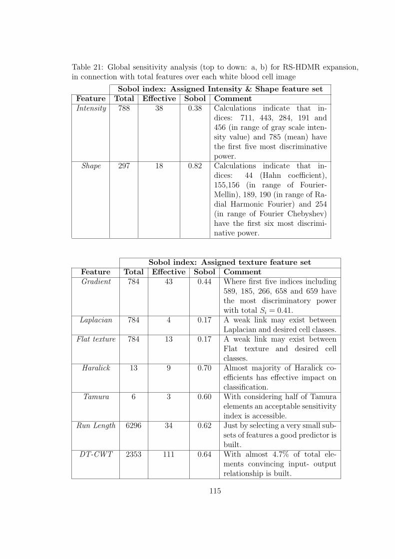
Table 21: Global sensitivity analysis (top to down: a, b) for RS-HDMR expansion,in connection with total features over each white blood cell image
Sobol index: Assigned Intensity & Shape feature setFeature Total Effective Sobol CommentIntensity 788 38 0.38 Calculations indicate that in-
dices: 711, 443, 284, 191 and456 (in range of gray scale inten-sity value) and 785 (mean) havethe first five most discriminativepower.
Shape 297 18 0.82 Calculations indicate that in-dices: 44 (Hahn coefficient),155,156 (in range of Fourier-Mellin), 189, 190 (in range of Ra-dial Harmonic Fourier) and 254(in range of Fourier Chebyshev)have the first six most discrimi-native power.
Sobol index: Assigned texture feature setFeature Total Effective Sobol CommentGradient 784 43 0.44 Where first five indices including
589, 185, 266, 658 and 659 havethe most discriminatory powerwith total Si = 0.41.
Laplacian 784 4 0.17 A weak link may exist betweenLaplacian and desired cell classes.
Flat texture 784 13 0.17 A weak link may exist betweenFlat texture and desired cellclasses.
Haralick 13 9 0.70 Almost majority of Haralick co-efficients has effective impact onclassification.
Tamura 6 3 0.60 With considering half of Tamuraelements an acceptable sensitivityindex is accessible.
Run Length 6296 34 0.62 Just by selecting a very small sub-sets of features a good predictor isbuilt.
DT-CWT 2353 111 0.64 With almost 4.7% of total ele-ments convincing input- outputrelationship is built.
115
Chapter 7
Classification
Machine learning and pattern recognition play critical role in the digital medical
imaging field, including computer-aided diagnosis and medical image analysis. Medi-
cal pattern recognition essentially requires ”learning from samples”. Classification of
objects such as white blood cells into specific white blood cell classes based on input
features (e.g., shape, intensity, and texture) is obtained from segmented leukocyte
candidates. In white blood cell analysis, a well defined system is initially created as
an explanation of its features and then classifies the cell based on that after apply-
ing feature selection strategies such as sequential forward feature selection, improved
branch and bound algorithm and high dimensional model representation. The results
of white blood cell classification are not always perfect and numerous factors affect
the results. This work examines Convolutional Neural Networks (LeNet5) [117] and
support vector machine (SVM) [13] in connection with white blood cell classification.
7.1 Convolutional Neural Networks (LeNet5)
Traditional manual-designed feature extractors are typically computationally inten-
sive and need prior theoretical and practical knowledge of the problem at hand. They
often cannot process raw images directly, while in classification scenario, automatic
methods which can retrieve features directly from raw data are generally preferable.
These trainable automatic systems solve classification problems without prior knowl-
edge on the data and features. A convolutional neural network (CNN) is a multilayer
perception with a special topology containing more than one hidden layer. It allows
116
for automatic feature extraction within its architecture and has as input the raw data.
7.1.1 The Standard CNN Formulation
We will investigate Convolution Neural Networks [117] which are sensitive to the
topology of the images being classified. An CNN uses a feed-forward method for
neurons feeding and back propagation for parameters training. The main advantage
of the CNN approach is its ability to extract topological properties from the raw
gray-scale image automatically and generate a prediction to classify high-dimensional
patterns. An CNN is composed of two distinct parts. The first part consists of
several layers that extract features from the input image pattern by a composition
of convolutional and sub-sampling layers. Conceptually, visual features from local
receptive fields [117] are extracted by an extended 2D convolution approach to gain
the appropriate spatially local correlation present in the input images. Since the
precise location of an extracted feature is in-consequent and dispensable, resolution
reduction by 2 of the features is followed through the sub-sampling layers. The second
distinct part categorizes the pattern into classes. In general, an CNN consists of three
different layers: convolution layer, sub-sampling (max-pooling) layer and an ensemble
of fully connected layers.
7.1.2 Literature Survey
There is a considerable amount of literature dedicated to using convolutional neural
network (CNN), starting with Lawrence et al. [118] in 1997 presenting a hybrid neural
network solution to automate facial feature detection. In last decade, CNN is very of-
ten used in different signal detection applications. The CNN has been used for object
recognition [121] and handwriting character recognition [117, 119, 210]. Simard [210]
examined various neural networks performance on visual handwriting recognition
tasks. Applications range from FAX documents, to analysis of scanned documents
and MNIST [120] data set.
Lauer et al. [117] introduced a trainable feature extractor based on convolutional
neural network to recognize handwritten digits. The results on the MNIST data set
showed that the system provided performances comparable in a black box data with-
out prior knowledge. Cecotti et al. [26] presented a model based on a convolutional
117
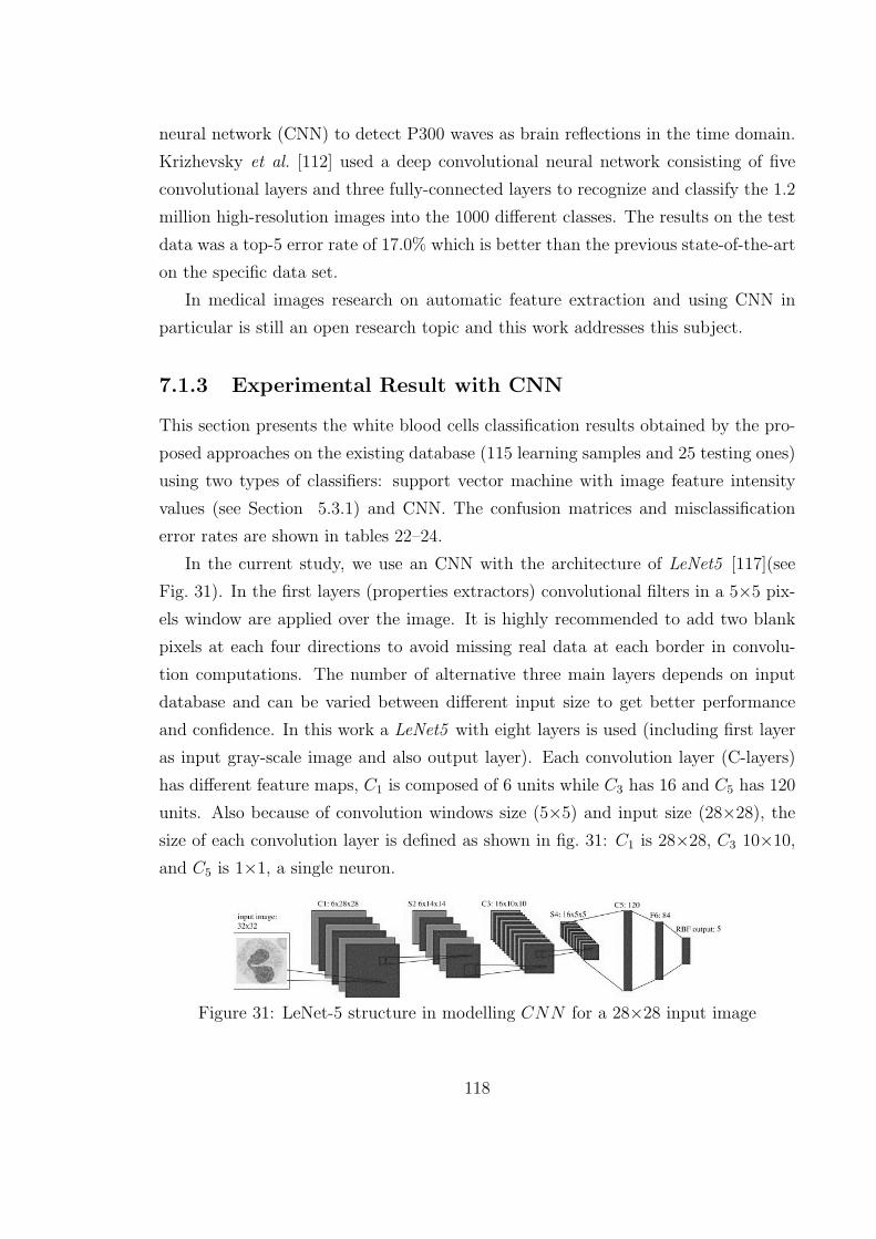
neural network (CNN) to detect P300 waves as brain reflections in the time domain.
Krizhevsky et al. [112] used a deep convolutional neural network consisting of five
convolutional layers and three fully-connected layers to recognize and classify the 1.2
million high-resolution images into the 1000 different classes. The results on the test
data was a top-5 error rate of 17.0% which is better than the previous state-of-the-art
on the specific data set.
In medical images research on automatic feature extraction and using CNN in
particular is still an open research topic and this work addresses this subject.
7.1.3 Experimental Result with CNN
This section presents the white blood cells classification results obtained by the pro-
posed approaches on the existing database (115 learning samples and 25 testing ones)
using two types of classifiers: support vector machine with image feature intensity
values (see Section 5.3.1) and CNN. The confusion matrices and misclassification
error rates are shown in tables 22–24.
In the current study, we use an CNN with the architecture of LeNet5 [117](see
Fig. 31). In the first layers (properties extractors) convolutional filters in a 5×5 pix-
els window are applied over the image. It is highly recommended to add two blank
pixels at each four directions to avoid missing real data at each border in convolu-
tion computations. The number of alternative three main layers depends on input
database and can be varied between different input size to get better performance
and confidence. In this work a LeNet5 with eight layers is used (including first layer
as input gray-scale image and also output layer). Each convolution layer (C-layers)
has different feature maps, C1 is composed of 6 units while C3 has 16 and C5 has 120
units. Also because of convolution windows size (5×5) and input size (28×28), the
size of each convolution layer is defined as shown in fig. 31: C1 is 28×28, C3 10×10,
and C5 is 1×1, a single neuron.
Figure 31: LeNet-5 structure in modelling CNN for a 28×28 input image
118
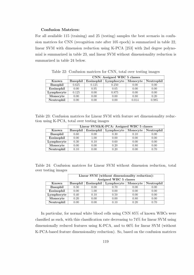
Confusion Matrices:
For all available 115 (training) and 25 (testing) samples the best scenario in confu-
sion matrices for CNN (recognition rate after 105 epoch) is summarized in table 22,
linear SVM with dimension reduction using K-PCA [253] with 2nd degree polyno-
mial is summarized in table 23, and linear SVM without dimensionality reduction is
summarized in table 24 below.
Table 22: Confusion matrices for CNN, total over testing images
CNN: Assigned WBC 5 classesKnown Basophil Eosinophil Lymphocyte Monocyte Neutrophil
Basophil 0.625 0.125 0.250 0.00 0.00Eosinophil 0.00 0.95 0.05 0.00 0.00
Lymphocyte 0.125 0.00 0.875 0.00 0.00Monocyte 0.00 0.00 0.00 0.80 0.20Neutrophil 0.00 0.00 0.00 0.014 0.985
Table 23: Confusion matrices for Linear SVM with feature set dimensionality reduc-tion using K-PCA, total over testing images
Linear SVM&K-PCA: Assigned WBC 5 classesKnown Basophil Eosinophil Lymphocyte Monocyte Neutrophil
Basophil 0.60 0.00 0.30 0.10 0.00Eosinophil 0.00 1.00 0.00 0.00 0.00
Lymphocyte 0.30 0.10 0.60 0.00 0.00Monocyte 0.00 0.00 0.20 0.80 0.00Neutrophil 0.10 0.00 0.20 0.00 0.70
Table 24: Confusion matrices for Linear SVM without dimension reduction, totalover testing images
Linear SVM (without dimensionality reduction):Assigned WBC 5 classes
Known Basophil Eosinophil Lymphocyte Monocyte NeutrophilBasophil 0.30 0.00 0.70 0.00 0.00
Eosinophil 0.00 1.00 0.00 0.00 0.00Lymphocyte 0.40 0.10 0.50 0.00 0.00Monocyte 0.20 0.00 0.00 0.80 0.00Neutrophil 0.00 0.00 0.10 0.20 0.70
In particular, for normal white blood cells using CNN 85% of known WBCs were
classified as such, with this classification rate decreasing to 74% for linear SVM using
dimensionally reduced features using K-PCA, and to 66% for linear SVM (without
K-PCA-based feature dimensionality reduction). So, based on the confusion matrices
119
with five classes the proposed CNN classifier is much more reliable and accurate even
in presence of similarity among classes (specially between Basophil and Lymphocyte)
in this difficult database yielding acceptable accuracy when compared to SVM (com-
pare the third diagonal entries in confusion matrices with (Lymphocyte) classification
rate =87% versus 60%).
CNN yields a false positive rate (FPR) of 14%, i.e., the proportion of negatives
samples incorrectly classified as positive, with this FPR increasing to 23% for linear
SVM using dimensionally reduced features using K-PCA, and then to 31% for linear
SVM (without using feature dimensionality reduction via K-PCA). The FPR of CNN
is also smaller than the FPR of a SVM using kernel PCA and it again confirms the
effectiveness of automatic feature extraction by CNN.
The CNN classifier has the acceptable accuracy by optimizing the topological
features on a difficult database containing small WBCs with no restrictions on back-
ground or capturing conditions. Experimental results indicate that a system based
on an CNN offers an improved recognition accuracy even in presence of poor quality
samples and multiple classes. Another advantage of CNN it extracts features au-
tomatically while in most other classifiers the features are chosen by the designer.
It is expected that classification accuracy will be further improved by extending the
data set size (especially to avoid confusion between Basophil & Lymphocyte cells since
their shapes are very similar in small magnification images) and also by optimizing
the CNN structure to reach higher performance in training and testing. However,
CNN-based systems are very slow convergence of the loss during training particularly
when the number of iterations increases during the training. These systems can be
difficult to implement and are usually slower than typical classifiers.
It should be noted that in CNN the most common method to reduce over-fitting on
this limited image data and also to reach better performance is to artificially enlarge
the dataset using different transformations that can be addressed for future work.
7.2 Support Vector Machine(SVM)
Studies and results indicate that support vector machine analysis offers remarkable
recognition accuracy even in presence of low number of samples and multiple classes.
Advances in implementation result is the possibility of extending the use of this
120
classifier to quantitatively measure the subtypes of cells (sub-differentiation) in the
entire field of haematology analysis.
7.2.1 The Standard SVM Formulation
Support vector machines are an example of a well-known linear/non-linear two-class
classifier. Let the notation xi (patterns) be the ith vector in a dataset sample (xi, yi)ni=1
where yi is the label associated with xi. A linear discriminant function is defined
implicitly by f(x) = ωTx + b. A simple and naive non-linear classifier is obtained
by mapping data from the input space using f(x) = ωTϕ(x) + b where ϕ is a kernel
mapping function. A linear combination of the training samples can be expressed
as the weight vector ω =∑n
i αixi. The classifier in non-linear approach takes the
form: f(x) =∑n
i αiϕ(xi)Tϕ(x)+b. The maximum margin classifier in support vector
machine is the discriminant function that maximizes the geometric margin 1∥ω∥ . To
allow errors and misclassified inputs, the optimization problem can be formulated as
a minimization over ω and b of the function 12∥ω∥2+C
∑ni=1 ζi, where C is a constant
value, subject to the inequality constraints yi(ωTxi + b) > 1 − ζi, and ζi ≥ 0. This
optimization problem can be solved in dual form using the Lagrange multipliers as
follows [13]. More detailed mathematical treatment of SVM and its implementations
can be found in [13,117].
7.2.2 Literature review
There are increasing evidences that prove support vector machines are being advan-
taged and popular in image classification. It has long clinical classification success in
use. Numerous studies have attempted to explain SVM in medical imaging such as
found in [47,54,111,129,183,220].
7.2.3 Experimental Result with SVM
Support vector machine (SVM) as a popular classification can efficiently perform
non-linear with using kernel trick in biomedical and biological applications. Common
kernel functions addressed are sigmoidal, polynomial kernels and radial basis functions
(RBFs) where kernel parameters have a direct impact on the decision boundary of the
support vector machine [13]. The lowest degree polynomial (polynomial with D = 1)
121
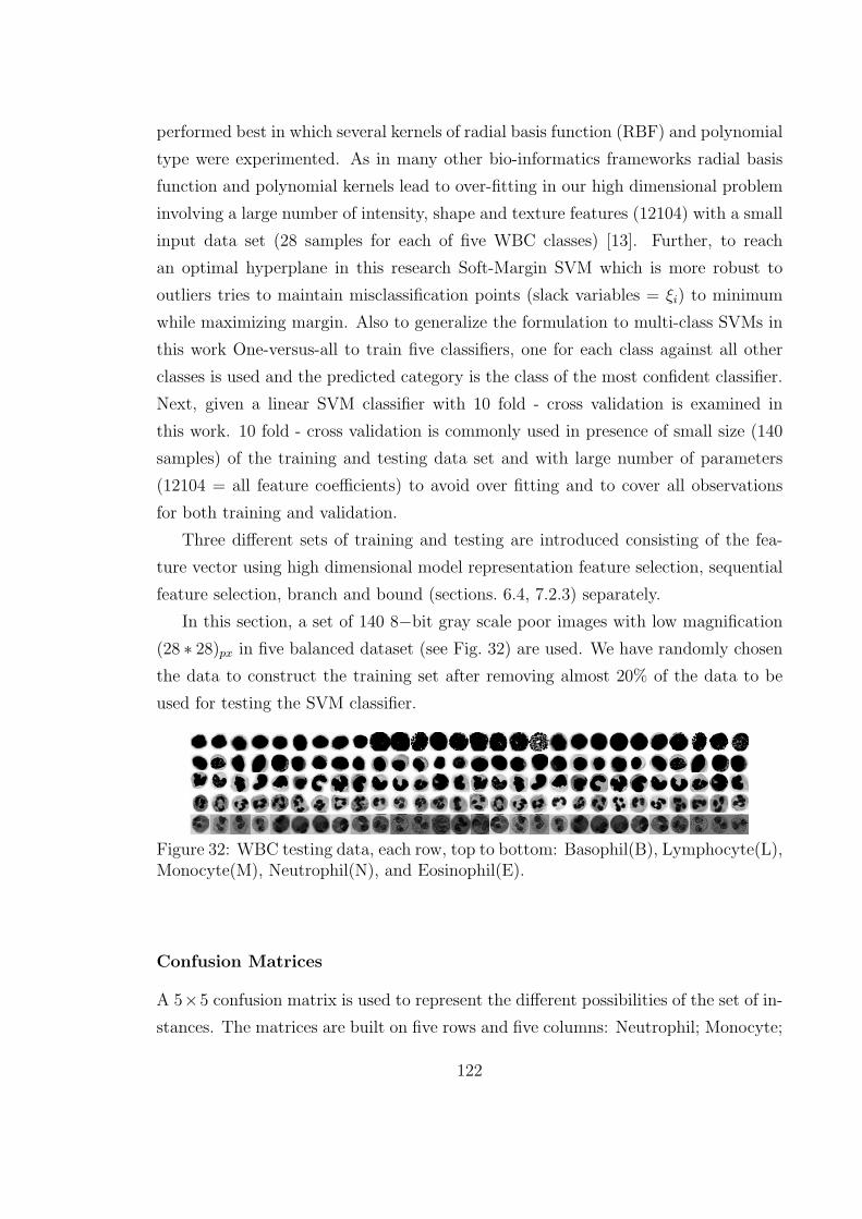
performed best in which several kernels of radial basis function (RBF) and polynomial
type were experimented. As in many other bio-informatics frameworks radial basis
function and polynomial kernels lead to over-fitting in our high dimensional problem
involving a large number of intensity, shape and texture features (12104) with a small
input data set (28 samples for each of five WBC classes) [13]. Further, to reach
an optimal hyperplane in this research Soft-Margin SVM which is more robust to
outliers tries to maintain misclassification points (slack variables = ξi) to minimum
while maximizing margin. Also to generalize the formulation to multi-class SVMs in
this work One-versus-all to train five classifiers, one for each class against all other
classes is used and the predicted category is the class of the most confident classifier.
Next, given a linear SVM classifier with 10 fold - cross validation is examined in
this work. 10 fold - cross validation is commonly used in presence of small size (140
samples) of the training and testing data set and with large number of parameters
(12104 = all feature coefficients) to avoid over fitting and to cover all observations
for both training and validation.
Three different sets of training and testing are introduced consisting of the fea-
ture vector using high dimensional model representation feature selection, sequential
feature selection, branch and bound (sections. 6.4, 7.2.3) separately.
In this section, a set of 140 8−bit gray scale poor images with low magnification
(28 ∗ 28)px in five balanced dataset (see Fig. 32) are used. We have randomly chosen
the data to construct the training set after removing almost 20% of the data to be
used for testing the SVM classifier.
Figure 32: WBC testing data, each row, top to bottom: Basophil(B), Lymphocyte(L),Monocyte(M), Neutrophil(N), and Eosinophil(E).
Confusion Matrices
A 5×5 confusion matrix is used to represent the different possibilities of the set of in-
stances. The matrices are built on five rows and five columns: Neutrophil; Monocyte;
122
Lymphocyte; Eosinophil; and Basophil representing the known WBC classes whereas
for each matrix, each row the values are normalized to sum to 1. Several standard
performance terms such as true positive rate or the recall (correctly identified- TP ),
false positive rate (incorrectly identified- FP ), true negative rate (correctly rejected-
TN), false negative rate (incorrectly rejected- FN), accuracy (proportion of the total
corrected predictions - AC), precision (proportion of the corrected predicted positive
cases -P ) have been extracted for the confusion matrix. This work addresses kappa
(κ) measure as it provides accuracy (AC) versus precision (P ) interpretation across
class categories [116]. Common Cohen’s un-weighted κ interpretation is:
≤ 0 ⇒ Poor
[0, 0.20] ⇒ Slight
[0.21, 0.40] ⇒ Fair
[0.41, 0.60] ⇒ Moderate
[0.61, 0.80] ⇒ Substantial
[0.81, 1.00] ⇒ AlmostPerfect
The experiments are categorized into set of named selected 273 out of 12140 features
(FVSFS, FVBB and FVHDMR) also with a total high dimensional feature vector with
12140 members (FVTotal).
Statistical performance measure is analyzed using analysis of confusion matrices
for each named feature & SVM summarized in tables 25a, 25b, 25c and 25d. Further
statistical tests revealed that given a small number of input samples (140) in high
dimensional feature sets (= 12140) using non-linear SVM kernels leads to over-fitting.
The result, as shown in table 25, indicates that for normal low resolution white
blood cells using linear SVM & all feature vector FVTotal 85% of known white blood
cells were classified as such, with this classification rate decreasing to 83.5% for FVBB
and 83% for (FVHDMR) (see Table 25 b,d) where the efficiency of (FVSFS) is also 81%
which is less than proposed Sobol - HDMR with 83%. RS-HDMR classification perfor-
mance with 273 elements is less and more similar where classification accuracy is also
found with all 12140 coefficients and with improved branch and bound method [98]
are selected. As confusion matrix tables illustrate, in this poor imaginary database
there is not a significant difference between for example the all high dimensional data
set and feature selected group with RS-HDMR expansion.
123
However, in general RS-HDMR and ”improved branch and bound” are more effi-
cient than SFS; and RS-HDMR is superior to both of the above mentioned methods.
All these three methods conducted a series of trials where they are different in both
their basis functions and the way they find a solution for the problem.
First, RS-HDMR selected feature vector is based on sobol calculation where the
number of efficient principal coefficients are up (i.e, 273 in this work) to reach first
order of sensitivity index (Si) value close to zero (more comments in [4, 267]). Sec-
ondly, feature subset selection in improved downwards branch and bound [98] is based
on least squares regression between invariant features and dependent white blood cell
class where subset size to be selected is under user decision. Both these two aforemen-
tioned cases are total independent tasks before classifier involving. Following that,
SFS method is a combination technique where its result is dependent on different
initial setting for classifier and its scalar return value criterion. Also, it is appar-
ent that the number of selected futures are manually assigned by user where unlike
the RS-HDMR there is no way to look over to degree of sensitivity of all individual
features.
The results, as shown in confusion matrix tables indicate that also HDMR results
for almost each sub-group is more accurate than SFS method where also sequential
forward selection algorithm is too dependent to classifier feedback as well.
Also with compare with two ground truth groups, using machines Sysmex XE-
series and also Abbott CELL-DYN range (see Section 2.1) it can be seen from the
data in confusion matrix tables that global sensitivity with Sobol on RS-HDMR ex-
pansion reveals 91% accuracy for Neutrophil, 65% rate for Lymphocyte and also 100%
for Eosinophil while the expensive machines mentioned above provide 92.5%, 92.2%,
and 87.7%, respectively in an ideal performance. It also provides 81% classification
rate for Monocytes and 77% for Basophils where the results obtained from machines
are 75.6% and 76.3%. The following conclusions in regard to κ coefficient can be also
drawn from the present confusion matrices. The Cohen’s unweighted κ coefficient of
the FVTotal, FVSFS, FVBB also FVHDMR are acceptable (0.81= almost perfect and
0.77, 0.79 = substantial) in this low resolution WBC classification. Taken together,
the most obvious finding to emerge from feature selection and with RS- HDMR study
in particular is that all these two methods provide substantial performance where
124
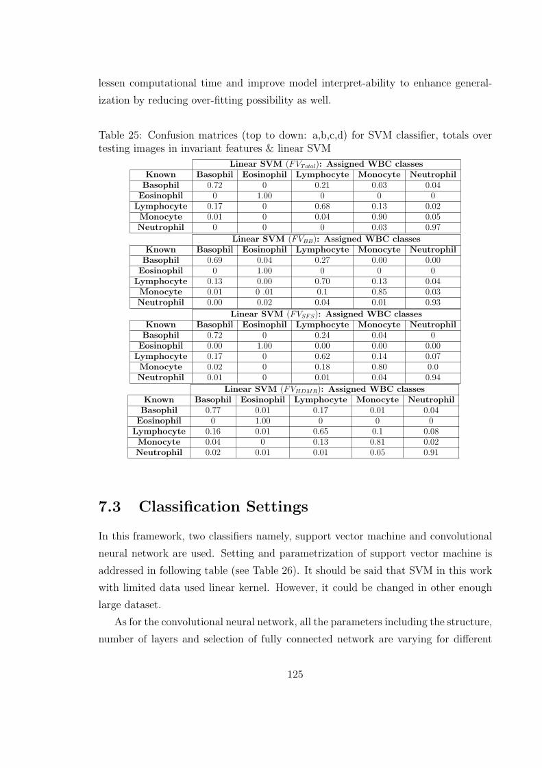
lessen computational time and improve model interpret-ability to enhance general-
ization by reducing over-fitting possibility as well.
Table 25: Confusion matrices (top to down: a,b,c,d) for SVM classifier, totals overtesting images in invariant features & linear SVM
Linear SVM (FVTotal): Assigned WBC classesKnown Basophil Eosinophil Lymphocyte Monocyte Neutrophil
Basophil 0.72 0 0.21 0.03 0.04Eosinophil 0 1.00 0 0 0
Lymphocyte 0.17 0 0.68 0.13 0.02Monocyte 0.01 0 0.04 0.90 0.05Neutrophil 0 0 0 0.03 0.97
Linear SVM (FVBB): Assigned WBC classesKnown Basophil Eosinophil Lymphocyte Monocyte Neutrophil
Basophil 0.69 0.04 0.27 0.00 0.00Eosinophil 0 1.00 0 0 0
Lymphocyte 0.13 0.00 0.70 0.13 0.04Monocyte 0.01 0 .01 0.1 0.85 0.03Neutrophil 0.00 0.02 0.04 0.01 0.93
Linear SVM (FVSFS): Assigned WBC classesKnown Basophil Eosinophil Lymphocyte Monocyte Neutrophil
Basophil 0.72 0 0.24 0.04 0Eosinophil 0.00 1.00 0.00 0.00 0.00
Lymphocyte 0.17 0 0.62 0.14 0.07Monocyte 0.02 0 0.18 0.80 0.0Neutrophil 0.01 0 0.01 0.04 0.94
Linear SVM (FVHDMR): Assigned WBC classesKnown Basophil Eosinophil Lymphocyte Monocyte Neutrophil
Basophil 0.77 0.01 0.17 0.01 0.04Eosinophil 0 1.00 0 0 0
Lymphocyte 0.16 0.01 0.65 0.1 0.08Monocyte 0.04 0 0.13 0.81 0.02Neutrophil 0.02 0.01 0.01 0.05 0.91
7.3 Classification Settings
In this framework, two classifiers namely, support vector machine and convolutional
neural network are used. Setting and parametrization of support vector machine is
addressed in following table (see Table 26). It should be said that SVM in this work
with limited data used linear kernel. However, it could be changed in other enough
large dataset.
As for the convolutional neural network, all the parameters including the structure,
number of layers and selection of fully connected network are varying for different
125
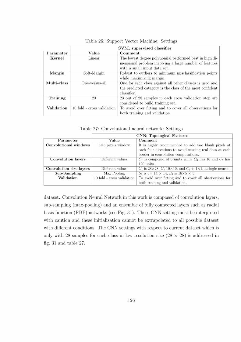
Table 26: Support Vector Machine: Settings
SVM; supervised classifierParameter Value Comment
Kernel Linear The lowest degree polynomial performed best in high di-mensional problem involving a large number of featureswith a small input data set.
Margin Soft-Margin Robust to outliers to minimum misclassification pointswhile maximizing margin.
Multi-class One-versus-all One for each class against all other classes is used andthe predicted category is the class of the most confidentclassifier.
Training 23 23 out of 28 samples in each cross validation step areconsidered to build training set.
Validation 10 fold - cross validation To avoid over fitting and to cover all observations forboth training and validation.
Table 27: Convolutional neural network: Settings
CNN; Topological FeaturesParameter Value Comment
Convolutional windows 5×5 pixels window It is highly recommended to add two blank pixels ateach four directions to avoid missing real data at eachborder in convolution computations.
Convolution layers Different values C1 is composed of 6 units while C3 has 16 and C5 has120 units.
Convolution size layers Different values C1 is 28×28, C3 10×10, and C5 is 1×1, a single neuron.Sub-Sampling Max Pooling S2 is 6× 14 × 14, S4 is 16×5 × 5.
Validation 10 fold - cross validation To avoid over fitting and to cover all observations forboth training and validation.
dataset. Convolution Neural Network in this work is composed of convolution layers,
sub-sampling (max-pooling) and an ensemble of fully connected layers such as radial
basis function (RBF) networks (see Fig. 31). These CNN setting must be interpreted
with caution and these initialization cannot be extrapolated to all possible dataset
with different conditions. The CNN settings with respect to current dataset which is
only with 28 samples for each class in low resolution size (28 × 28) is addressed in
fig. 31 and table 27.
126
Chapter 8
Conclusions and Future Work
There are many challenging problems in automatic processing of cytological of image
blood cells. The main problems include large variation of blood cells, occlusions,
low quality of images and difficulties in getting enough real data. These problems
are addressed in this work. In this work, a step-by-step efficient segmentation and
classification algorithm have been presented automatic detection and segmentation of
microscopic blood imagery. Experimental results indicate that our system offers good
segmentation and recognition accuracy with normal samples. The performance of the
proposed method has been evaluated by comparing the automatically extracted cells
with manual segmentations by a pathologist from GHODS polyclinic (Tehran, Iran).
In this work, a framework divided into four main stages: image pre-processing, feature
extraction, feature selection and classification is proposed. We provide literature
survey and point out new challenges.
First, a reliable pre-processing system that may be used under different conditions
(such as low quality, unfavourable resolution, varying inconsistent illumination condi-
tions and also the complexity staining techniques) is introduced. Next, separation of
different cells as well as the identification of RBC and WBC is resolved. An efficient
and highly accurate local binarization method is introduced here. Cell separation is
accomplished using cutting edge image segmentation and boundary detection tech-
niques in combination with morphological techniques with the goal of improving the
accuracy of complete blood count (CBC). The available data is poor quality and
therefore shape and inside structures are difficult to estimate. These conditions in-
clude noisy low resolution blood smear images. White blood cells texture, cytoplasm
127
and membrane are non-uniform staining and granular white blood cell shapes are also
difficult to detect. As a result, we have introduced efficient invariant shape, intensity
and texture features for white blood cells classification in this difficult dataset with
low resolution images.
Statistical measures were used to investigate redundancy and relevance of features.
They include Kolmogorov - Smirnov (KS) and Wilcoxon- Mann-Whitney (WMW)
tests, Pearson, Spearman and Kendall rank correlation coefficients. These statical
tests show a low degree of redundancy among these features. Almost all aforemen-
tioned features (except for Legendre moments) are independent and there is no re-
dundant information in them. Furthermore, this work concentrates on usefulness of
feature selection in presence of big data with high dimensional invariant features in
connection with white blood cell classification. In our work on white blood cell classi-
fication features vectors have 12140 components and lot of effort is devoted to feature
selection. This work examines and presents the effectiveness of three methods such as
sequential feature selection (SFS) set, improved branch and bound (BB) and random
sample high-dimensional model representation (RS-HDMR). RS-HDMR using Sobol
rank calculation automatically detected 273 best features and then we used sequential
feature selection (SFS) set, improved branch and bound (BB) to select the best 273
features as well.
All these three SFS, RS-HDMR and ”improved branch and bound” substitute
large number of features (D12104) to subset of features (D273) to avoid curse of dimen-
sionality, reduce feature measurement and computational burden and then recall the
SVM classifier based on these selected features.
We subsequently tested the set of selected features using SVM and determined
that RS-HDMR produced the most discriminatory features. These findings suggest
that, in general, RS-HDMR emerged as a reliable input-output relationship predictor
of small distorted WBCs and their own classes to allow the full feature sensitivity
analysis based on Sobol sequences.
One of the more significant findings to emerge from this study is the possibility
of extending this framework to entire field of hematology analysis, stool examination
or other similar medical research. Furthermore, the introduced method being simple
and easy to implement is best suited for biomedical applications in clinical settings.
This work aims at development of publicly available software for complete blood
128
count test for automatic processing of blood slide images. Of course with good recog-
nition accuracy even in presence of low resolution images and noise.
8.1 Original Contributions of the Thesis
The thesis addresses the problem of segmentation and counting red blood cells along
with classification of cytological images of white blood cells in peripheral blood smear
for complete blood count (CBC) test. In this concept, this study made an effort to
reach a framework to extract blood test parameters even in presence of low resolution
images. This work calculates main CBC test indices such as RBC count, red cell
distribution width (RDW), WBC Count and WBC differential (see Section. 1.2.1).
The main contribution of this study is in forming a complete framework of method-
ologies and procedures required for automatic processing of normal blood slide images
for complete blood count diagnosis test. The system is able to process the low reso-
lution and degraded images where manual analysis of microscopic blood slides which
is not only a tedious task and but also likely to fail or make human errors.
This section lists main achievements of the thesis. The finding of this work points
out some contributions to the literature in normal blood segmentation and classifica-
tion.
• More accurate white blood cells classification in presence of low quality images.
• The introduction of using semi-interquartile range, variance statistical approach
to reach channel color selection criteria in presence of different gray scale options
for blood smear microscopic images (see Section 3.2.1).
• Study and investigation of more accurate blood smear image pre-processing,
which it includes Bayesian Non-local means as image de-noising, utilizing Kauwahra
filter for white blood edge preserving (see Sections 3.2.2, 3.2.3).
• The introduction of an improved and more generalized binarization using merged
Niblack as local and Otsu as global techniques to improve foreground/background
segmentation of blood smear microscopic images (see Section 4.3.1).
• Study and investigation of white blood cell image separation using improved ac-
tive contour model without an edge, morphological operations and edged images
129
for blood cells separation in presence of degraded images (see Section 4.3.1).
• A comprehensive study and introduction of a set of appropriate invariant high
dimensional feature coefficients such as invariant orthogonal moments, Dual-
Tree Complex Wavelet Transform, Run-length for classification of blood smear
microscopic images (see Section 5.3).
• Study and investigation of the redundancy and distribution behaviour of these
named invariant features with approaches such as Kolmogorov - Smirnov (KS),
Wilcoxon- Mann-Whitney (WMW) tests, Spearman and Kendall rank correla-
tion coefficients for blood smear microscopic images (see Section 5.6).
• Study and investigation of feature selection to provide effective reduction of fea-
ture vector size for classification of blood smear microscopic images. Global sen-
sitivity analysis with combination of random sampling-high dimensional model
representation (RS-HDMR) and Sobol sensitivity analysis to assess discrimi-
natory power and rank of each individual feature is addressed (section 6.1,
table 21).
• The comparison of set of classifiers such as support vector machine (SVM),
Convolutional Neural Networks (CNN) to evaluate their performance to distin-
guish between inter-classes for classification of white blood cells in blood smear
microscopic images. This work extracts topological features by Convolutional
Neural Networks (LeNet5) to separate white blood cell classes (see Sections 5.3,
7.1.3, 7.2.3).
Aforementioned sub-sections explain original contributions of this thesis in more
detail. Blood smear image pre-processing findings are addressed in section 3.4. The
original contribution emerges from Binarization & blood cell separation are found in
section 4.5.
Finally I applied feature extraction & selection algorithms to obtain good discrim-
inative features for white blood cells classification, see discussion in sections 5.7, 6.6.
130
8.2 Publications of the Author
The aim of [78] was to introduce an accurate mechanism for counting blood smear
particles. This is accomplished by using the Immersion Watershed algorithm which
counts red and white blood cells separately. To evaluate the capability of the proposed
framework, experiments were conducted on noisy normal blood smear images. This
framework was compared to other published approaches and found to have lower
complexity and better performance in its constituent steps; hence, it has a better
overall performance.
In paper [113] we discuss applications of pattern recognition and image process-
ing to automatic processing and analysis of histopathological images. We focus on
two applications: counting of red and white blood cells using microscopic images of
blood smear samples and breast cancer malignancy grading from slides of fine needle
aspiration biopsies. We provide literature survey and point out new challenges.
In third article [72] we discuss improved binarization using merged Niblack and
Otsu techniques to improve foreground/background segmentation of blood smear mi-
croscopic images. We aim at more accuracy in terms of minimizing the number of
close pairs of cells that are merged into single cells during binarization process.
In conference work [75] a convolutional neural network (CNN) to extract topologi-
cal features is proposed. The proposed classifiers were compared through experiments
conducted on low resolution cytological images of normal blood smears
In [73] we particularly interested in classification and counting of the five main
types of white blood cells (leukocytes) in a clinical setting where the quality of micro-
scopic imagery may be poor. In this paper we implement a machine learning system
based on using extracting features by Dual-Tree Complex Wavelet and SVM as a
classifier.
In [74] we analyze the performance of white blood cell recognition system for three
different sets of features and these features are combined with the Support Vector
Machine (SVM) which classifies white blood cells into their five primary types. This
approach was validated with experiments conducted on digital normal blood smear
images with low resolution.
In conference work [76] we use a high dimensional vector addressing invariant
features. Global sensitivity analysis using Sobol RS-HDMR which can deal with
independent and dependent input variables is used to assess dominate discriminatory
131
power and the reliability of feature models in presence of high dimensional input
feature data to build an efficient feature selection.
Paper [77] has been submitted to Computers in Biology and Medicine Journal -
Elsevier. It is about feature extraction and selection for White Blood Cell differential
counts in low resolution cytological images. These work focus on the development of
effective strategies for the understanding of invariant feature extraction and then opti-
mal selection based on different statistically measured approaches on high-dimensional
feature data in low resolution images.
8.3 Challenges & Future Work
Automatic CBC (complete blood count) is a challenging and unsolved problem. It
involves classification of white blood cells into five main categories such as basophils,
eosinophils, lymphocytes, monocytes and neutrophils, and detection and categoriza-
tion of blood pathologies such as anemias, leukaemias, lymphomas, cholera, malaria
and many others. As different white blood cell and pathologies may be differenti-
ated by shape, texture, color and other visual cues advanced image processing and
machine learning techniques need to be utilized to build reliable classification sys-
tems. An important problem to address is the separation of different white blood cell
classes(mature and immature) into 20 sub-classes ”information about cellular imma-
turity ” such as mentioned in [67, Chapter 170]. It may be used to help monitor
more sophisticated cases, as well as the identification of deformed RBC and white
blood cell shapes with diseases [67]. Some red blood cell abnormalities case are listed
here ( [67], figures 160-2 to 160-15) :
I Macrocytic anemia : cells are larger than normal and oval in shape(arrow).
II Sickle cells : a sickle or crescent shape.
III Teardrop poikilocytes : Teardrop-shaped red cells.
IV Rouleau formation : chain of overlapped red cells. and etc.
Further research should be done to investigate the different techniques to address
better improvement in segmentation step. This will be accomplished using cutting
edge image segmentation techniques in combination with advanced machine learning
132
techniques for classification, with the goal of improving the accuracy of CBC reports
and to isolate cells in the individual sub images. The methods such as simultaneous
detection and segmentation [83] should be investigated. Feature selection is an im-
portant issue for future research. The findings are expected to be supported by future
work considering different underdeveloped HDMR variations, i.e., Sobol HDMR using
Quasi Monte Carlo, multiple sub-domain random sampling HDMR, or Cut-HDMR.
In this study it is assumed that the number of samples in each individual class is
identical and we have a balanced database in which in practice typical proportions
of the cell types are not the same in blood smear slides (e.g., neutrophil (40- 75%)
vs basophil granulocytes (0.5%)). In such cases, a Breiman Random Forest (BRF)
[23], deep belief networks and Restricted Boltzmann Machines classifiers may be
potentially useful. The BRF algorithm can deal with imbalanced data, can handle
more variables (features) than observations (large attributes, small sample), is robust
for data sets containing noisy samples, and has a good predictive ability without
over-fitting the data. Further, to extract a compact basis of discriminant training
samples, dictionary learning techniques and sparse coding to learn each species are
used. In particular, sparse coding and dictionary methods have proven to be efficient
at modeling complex structures and to be robust to noise, two essential abilities for
the target problem.
8.4 Acknowledgements
We would like to thank professor Nick Kingsbury from the University of Cambridge,
UK for providing his Dual-Tree Complex Wavelet Transform code. We also thank Dr.
Tilo Ziehn and professor Alison Tomlin from University of Leeds for providing a freely
available Matlab toolbox with a graphical user interface to global sensitivity analysis
of complex models. We also appreciate Aida Habibzadeh and M.D Parvaneh Saberian
whose comments and suggestions helped to improve and clarify this manuscript.
133
Chapter 9
Appendix - Images
This section contains image information, links to normal, blood cell disorders and
mature white blood cell classes.
9.1 Blood with Different Characteristics
134
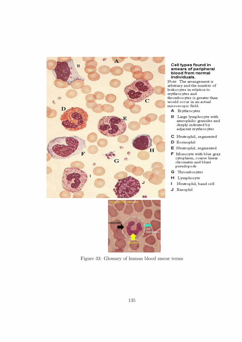
Figure 33: Glossary of human blood smear terms
135
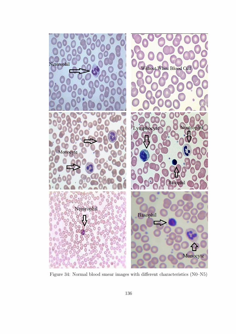
Figure 34: Normal blood smear images with different characteristics (N0–N5)
136
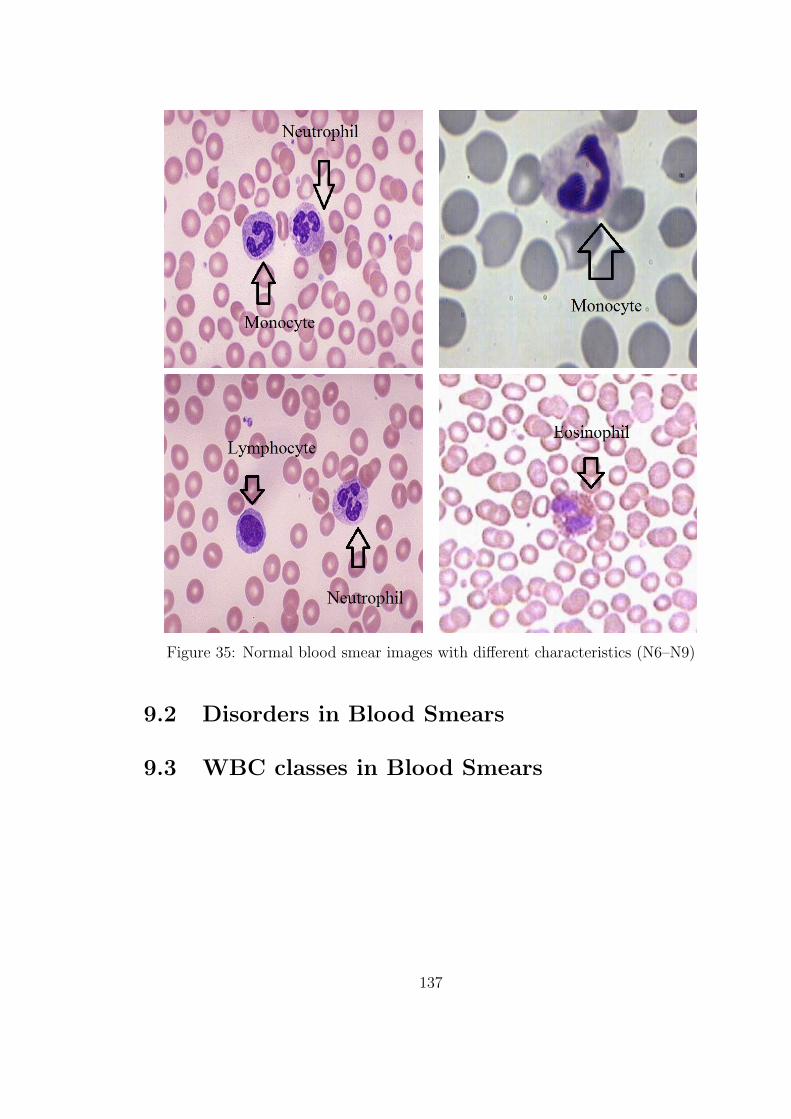
Figure 35: Normal blood smear images with different characteristics (N6–N9)
9.2 Disorders in Blood Smears
9.3 WBC classes in Blood Smears
137
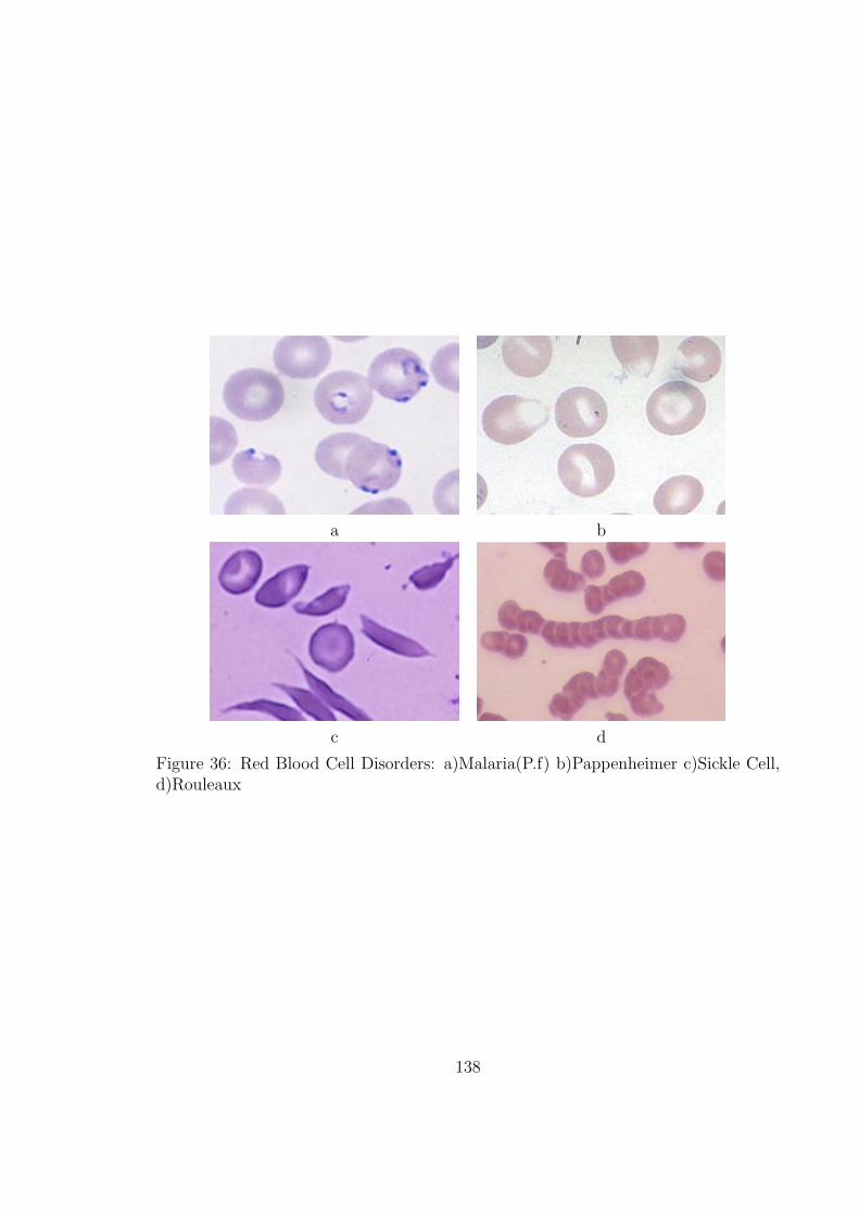
a b
c d
Figure 36: Red Blood Cell Disorders: a)Malaria(P.f) b)Pappenheimer c)Sickle Cell,d)Rouleaux
138
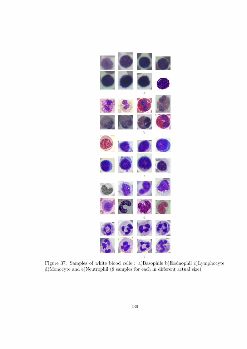
a
b
c
d
e
Figure 37: Samples of white blood cells : a)Basophils b)Eosinophil c)Lymphocyted)Monocyte and e)Neutrophil (8 samples for each in different actual size)
139
Bibliography
[1] M. Adjouadi and N. Fernandez. An orientation-independent imaging technique
for the classification of blood cells. Particle & Particle Systems Characteriza-
tion, 18(2):91–98, 2001.
[2] Sh. Ahmad, Q. Zhang, Z.M. Lu, and M.W. Anwar. Feature-based watermarking
using discrete orthogonal hahn moment invariants. In 7th International Con-
ference on Frontiers of Information Technology, FIT, pages 38:1–38:6, 2009.
[3] M. Albertini, L. Teodori, E. Piatti, M. Piacentini, A. Accorsi, and M. Roc-
chi. Automated analysis of morphometric parameters for accurate definition of
erythrocyte cell shape. Cytometry Part A, 52A(1):12–18, 2003.
[4] O. Alis and H. Rabitz. Efficient implementation of high dimensional model
representations. Journal of Mathematical Chemistry, 29(2):127–142, 2001.
[5] J.P. Ananth and V.S. Bharathi. Face image retrieval system using discrete
orthogonal moments. In 4th International Conference on Bioinformatics and
Biomedical Technology (IPCBEE), pages 218–223, 2012.
[6] G. Apostolopoulos, S. Tsinopoulos, and E. Dermatas. Recognition and identi-
fication of red blood cell size using Zernike moments and multicolor scattering
images. In 10th International Workshop on Biomedical Engineering, pages 1–4,
2011.
[7] R. Archibald, K. Chen, A. Gelb, and R. Renaut. Improving tissue segmentation
of human brain MRI through preprocessing by the gegenbauer reconstruction
method. NeuroImage, 20(1):489 – 502, 2003.
140
[8] R. Archibald, H. Jiuxiang, A. Gelb, and G. Farin. Improving the accuracy of
volumetric segmentation using pre-processing boundary detection and image
reconstruction. IEEE Transactions on Image Processing, 13(4):459–466, 2004.
[9] M.R. Asadi, A. Vahedi, and H. Amindavar. Leukemia cell recognition with
Zernike moments of holographic images. In Proceedings of the 7th Nordic Signal
Processing Symposium (NORSIG), pages 214–217, 2006.
[10] Z.V. Babic and D.P. Mandic. An efficient noise removal and edge preserving
convolution filter. In 6th International Conference on Telecommunications in
Modern Satellite, Cable and Broadcasting Service, volume 2, pages 538–541,
Oct. 2003.
[11] J.W. Bacusmber and E.E. Gose. Leukocyte pattern recognition. IEEE Trans-
actions on Systems, Man and Cybernetics, SMC-2(4):513–526, 1972.
[12] R.R. Bailey and M. Srinath. Orthogonal moment features for use with para-
metric and non-parametric classifiers. IEEE Transactions on Pattern Analysis
and Machine Intelligence, 18(4):389–399, 1996.
[13] A. Ben-Hur and J. Weston. A user guide to support vector machines. In Data
Mining Techniques for the Life Sciences, volume 609, pages 223–239, 2010.
[14] S. Bentley and S. Lewis. The use of an image analyzing computer for the quan-
tification of red cell morphological characteristics. British Journal of Hematol-
ogy, 29:81–88, 1975.
[15] T. Bergen, D. Steckhan, T. Wittenberg, and T. Zerfass. Segmentation of leuko-
cytes and erythrocytes in blood smear images. In 30th Annual International
Conference of the IEEE on Engineering in Medicine and Biology Society, pages
3075–3078, 2008.
[16] J. Bernsen. Dynamic thresholding of grey-level images. In International Con-
ference on Pattern Recognition, pages 1251–1255, 1986.
[17] H.S. Bhadauria and M.L. Dewal. Efficient Denoising Technique for CT images
to Enhance Brain Hemorrhage Segmentation. Journal of Digital Imaging, pages
1–10, 2012.
141
[18] S.F. Bikhet, A.M. Darwish, H.A. Tolba, and S.I. Shaheen. Segmentation and
classification of white blood cells. In IEEE International Conference on Acous-
tics, Speech, and Signal Processing(ICASSP), volume 6, pages 2259–2261, 2000.
[19] T.J. Bin, A. Lei, C. Jiwen, K. Wenjing, and L. Dandan. Subpixel edge location
based on orthogonal fourier-mellin moments. Image and Vision Computing,
26(4):563 – 569, 2008.
[20] B. Bobier and M. Wirth. Evaluation of binarization algorithms. Technical re-
port, Department of Computing and Information Science, University of Guelph,
Guelph, ON, 2008.
[21] S. Bouatmane, M. Roula, A. Bouridane, and S. Al-Maadeed. Round-robin se-
quential forward selection algorithm for prostate cancer classification and diag-
nosis using multispectral imagery. Machine Vision and Applications, 22(5):865–
878, 2011.
[22] D. Bradley and G. Roth. Adaptive thresholding using the integral image. Jour-
nal of Graphics, GPU, & Game Tools, 12(2):13 – 21, 2007.
[23] L. Breiman. Random forests. Machine Learning, 45(1):5–32, Oct. 2001.
[24] M. Buttarello and M. Plebani. Automated blood cell counts -state of the art.
American Journal of Clinical Pathology, 130:104–116, 2008.
[25] E.A. Castro and D.L. Donoho. Does Median filtering truly preserve edges better
than linear filtering? The Annals of Statistics, 37(3):1172 – 1206, 2009.
[26] H. Cecotti and A. Graser. Convolutional neural networks for P300 detection
with application to brain-computer interfaces. IEEE Transactions on Pattern
Analysis and Machine Intelligence, 33(3):433–445, Mar. 2011.
[27] J. Salmon Ch.A. Deledalle and A. Dalalyan. Image denoising with patch based
PCA: local versus global. In Proceedings of the British Machine Vision Con-
ference, pages 25.1–25.10. BMVA Press, 2011.
[28] H. Chan, J. Li-Jun, and B. Jiang. Wavelet transform and morphology image
segmentation algorism for blood cell. In 4th IEEE International Conference on
Industrial Electronics and Applications, pages 542 –545, May. 2009.
142
[29] T.F. Chan and L.A. Vese. Active contours without edges. IEEE Transactions
on Image Processing, 10(2):266 –277, Feb. 2001.
[30] S.G. Chang, B. Yu, and M. Vetterli. Adaptive wavelet thresholding for image
denoising and compression. IEEE Transactions on Image Processing, 9(9):1532–
1546, 2000.
[31] G.Y. Chen, T.D. Bui, and A. Krzyzak. Image denoising with neighbour depen-
dency and customized wavelet and threshold. Pattern Recognition, 38(1):115 –
124, 2005.
[32] C.K. Chow and T. Kaneko. Automatic boundary detection of the left ventricle
from cineangiograms. Computers and Biomedical Research, 5(4):388 – 410,
1972.
[33] J. L Coatrieux. Moment-based approaches in imaging part 2: invariance. IEEE
Engineering in Medicine and Biology Magazine, 27(1):81–83, 2008.
[34] D. Comaniciu and P. Meer. Cell image segmentation for diagnostic pathology.
In Advanced algorithmic approaches to medical image segmentation, pages 541–
558. Springer, , 2002.
[35] H. Costin, C. Rotariu, M. Zbancioc, M. Costin, and E. Hanganu. Fuzzy rule-
aided decision support for blood cell recognition. Fuzzy Systems & Artificial
Intelligence, 7(1-3):61–70, 2001.
[36] P. Coupe, P. Hellier, C. Kervrann, and C. Barillot. Nonlocal Means-Based
Speckle Filtering for Ultrasound Images. IEEE Transactions on Image Process-
ing, 18(10):2221–2229, Oct. 2009.
[37] A. Cramer. Bijdrage tot de quantitative mikroskopische analyse van het bloed.
Het tellen der bloedligchaampjes, 4(453), 1855.
[38] B. Dangott, M. Salama, N. Ramesh, and T. Tasdizen. Isolation and two-step
classification of normal white blood cells in peripheral blood smears. Journal
of Pathology Informatics, 3(1):13, 2012.
143
[39] D.K. Das, C. Chakraborty, B. Mitra, A.K. Maiti, and A.K. Ray. Quantitative
microscopy approach for shape-based erythrocytes characterization in anaemia.
Journal of Microscopy, 249(2):136–149, 2013.
[40] M. Portes de Albuquerque, I.A. Esquef, A.R. Gesualdi Mello, and M. Portes
de Albuquerque. Image thresholding using Tsallis entropy. Pattern Recognition
Letters, 25(9):1059 – 1065, 2004.
[41] A G. Dempster and C. Di Ruberto. Using granulometries in processing images
of malarial blood. In IEEE International Symposium on Circuits and Systems,
volume 5, pages 291–294, 2001.
[42] Z. Dengwen and Ch. Wengang. Image denoising with an optimal threshold and
neighbouring window. Pattern Recognition Letters, 29(11):1694 – 1697, 2008.
[43] C. Desbleds-Mansard, A. Anwander, L. Chaabane, M. Orkisz, B. Neyran,
P. Douek, and I. Magnin. Dynamic active contour model for size independent
blood vessel lumen segmentation and quantification in high-resolution magnetic
resonance images. In Computer Analysis of Images and Patterns, volume 2124
of Lecture Notes in Computer Science, pages 264–273. Springer Berlin Heidel-
berg, 2001.
[44] C. Di Ruberto, A. Dempster, S. Khan, and B. Jarra. Segmentation of blood
images using morphological operators. In 15th IEEE International Conference
on Pattern Recognition (ICPR), pages 397–400, 2000.
[45] C. Di Ruberto, A. Dempster, S. Khan, and B. Jarra. Analysis of infected
blood cell images using morphological operators. Image and Vision Computing,
20(2):133–146, 2002.
[46] C. Di Ruberto, A. Dempster, Sh. Khan, and B. Jarra. Morphological image
processing for evaluating malaria disease. In Visual Form, volume 2059 of
Lecture Notes in Computer Science, pages 739–748. Springer Berlin, Heidelberg,
2001.
[47] A. P. Dobrowolski, M. Wierzbowski, and K. Tomczykiewicz. Multiresolu-
tion MUAPs decomposition and SVM-based analysis in the classification of
144
neuromuscular disorders. Computer Methods and Programs in Biomedicine,
107(3):393 – 403, 2012.
[48] G. Dong, N. Ray, and S.T. Acton. Intravital leukocyte detection using the
gradient inverse coefficient of variation. IEEE Transactions on Medical Imaging,
24(7):910–924, Jul. 2005.
[49] D.L. Donoho. De-noising by soft-thresholding. IEEE Transactions on Informa-
tion Theory, 41(3):613–627, 1995.
[50] D.L. Donoho and I.M. Johnstone. Adapting to unknown smoothness via wavelet
shrinkage. Journal of the American Statistical Association, 90(432):1200–1224,
1995.
[51] L.B. Dorini, R. Minetto, and N.J. Leite. Semi-automatic white blood cell seg-
mentation based on multiscale analysis. IEEE Journal of Biomedical and Health
Informatics, 17(1):250–256, 2013.
[52] S.R. Dubois and F.H. Glanz. An autoregressive model approach to two-
dimensional shape classification. IEEE Transactions on Pattern Analysis and
Machine Intelligence, 8(1):55–66, 1986.
[53] M.P. Dubuisson and A.K. Jain. A modified hausdorff distance for object match-
ing. In 12th IAPR International Conference on Pattern Recognition, volume 1,
pages 566–568, 1994.
[54] I. El-Naqa, Yongyi Y., M.N. Wernick, N.P. Galatsanos, and R.M. Nishikawa.
A support vector machine approach for detection of microcalcifications. IEEE
Transactions on Medical Imaging, 21(12):1552–1563, Dec. 2002.
[55] J. Fan, R. Wang, L. Zhang, D. Xing, and F. Gan. Image sequence segmenta-
tion based on 2D temporal entropic thresholding. Pattern Recognition Letters,
17(10):1101 – 1107, 1996.
[56] M.L. Feng and Y.P. Tan. Contrast adaptive binarization of low quality docu-
ment images. IEICE Electron. Express, 1(16):501 – 506, 2004.
145
[57] S. Fischer, F. sroubek, L. Perrinet, R. Redondo, and G. Cristbal. Self-invertible
2D Log-Gabor Wavelets. International Journal of Computer Vision, 75(2):231–
246, 2007.
[58] S. Fleagle, M. Johnson, C. Wilbricht, D. Skorton, R. Wilson, C. White, M. Mar-
cus, and S. Collins. Automated analysis of coronary arterial morphology in
cineangiograms: geometric and physiologic validation in humans. IEEE Trans-
actions on Medical Imaging, 8(4):387–400, 1989.
[59] S. Fleagle, D. Thedens, J. Ehrhardt, T. Scholz, and D. Skorton. Automated
identification of left ventricular borders from spin-echo magnetic resonance im-
ages. Investigative Radiology, 26(4):295–303, 1991.
[60] I. Fodor and C. Kamath. On denoising images using wavelet-based statistical
techniques. Technical report, Lawrence Livermore National Laboratory, 2001.
[61] H. Freeman. Computer processing of line-drawing images. ACM Computing
Surveys, 6(1):57–97, 1974.
[62] B. Fu, J. Zhou, Y. Li, G. Zhang, and Ch. Wang. Image analysis by modified
legendre moments. Pattern Recognition, 40(2):691 – 704, 2007.
[63] K. Fukunaga. Introduction to Statistical Pattern Recognition,second ed. Aca-
demic Press Inc, New York, NY, USA, 1992.
[64] B. Gatos, I. Pratikakis, and S. Perantonis. An adaptive binarization technique
for low quality historical documents. In Document Analysis Systems VI, volume
3163 of Lecture Notes in Computer Science, pages 102–113. Springer Berlin
Heidelberg, 2004.
[65] B. Gatos, I. Pratikakis, and S.J. Perantonis. Adaptive degraded document
image binarization. Pattern Recognition, 39(3):317 – 327, 2006.
[66] E. Gering and C. Atkinson. A rapid method for counting nucleated erythrocytes
on stained blood smears by digital image analysis. Journal of Parasitology,
90(4):879–881, 2004.
[67] L. Gooldman and A. Schafer. The peripheral blood smear. In Cecil Medicine,
chapter 160. Saunders Elsevier, Philadelphia, Pa, 24 edition, 2011.
146
[68] G.H. Granlund. Fourier preprocessing for hand print character recognition.
IEEE Transactions on Computers, C-21(2):195–201, 1972.
[69] E. Grimaldi and F. Scopacasa. Evaluation of the abbott CELL-DYN 4000
hematology analyzer. American Journal of Clinical Pathology, 113(4):497–505,
Apr. 2000.
[70] Yu-Hua Gu and T. Tjahjadi. Efficient planar object tracking and parameter es-
timation using compactly represented cubic B-spline curves. IEEE Transactions
on Systems, Man and Cybernetics, Part A: Systems and Humans, 29(4):358–
367, 1999.
[71] H. Taghizad E. Khajehpour H. Khajehpour, A. Mehri Dehnavi and M.R.
Naeemabadi. Detection and segmentation of erythrocytes in blood smear im-
ages using a line operator and watershed algorithm. Journal of Medical Signals
and Sensors, 3(3):164–171, Sept. 2013.
[72] M. Habibzadeh, A. Krzyzak, and T. Fevens. Application of pattern recognition
techniques for the analysis of thin blood smear images. Journal of Medical
Informatics & Technologies., 18(1):29–40, 2011.
[73] M. Habibzadeh, A. Krzyzak, and T. Fevens. Analysis of white blood cell dif-
ferential counts using dual-tree complex wavelet transform and support vector
machine classifier. In International Conference on Computer Vision and Graph-
ics (ICCVG), volume 7594, pages 414–422, Sept. , 2012.
[74] M. Habibzadeh, A. Krzyzak, and T. Fevens. Comparative study of shape,
intensity and texture features and support vector machine for white blood cell
classification. Journal of Theoretical and Applied Computer Science, 7:20–35,
2013.
[75] M. Habibzadeh, A. Krzyzak, and T. Fevens. White blood cell differential counts
using Convolutional Neural Networks for low resolution images. In Artificial
Intelligence and Soft Computing, volume 7895 of Lecture Notes in Computer
Science, pages 263–274. Springer Berlin Heidelberg, 2013.
[76] M. Habibzadeh, A. Krzyzak, and T. Fevens. Comparative Study of Feature
Selection for White Blood Cell Differential Counts in Low Resolution Images.
147
In Artificial Neural Networks in Pattern Recognition (ANNPR), volume 8774
of Lecture Notes in Computer Science, pages 216–227. Springer International
Publishing Switzerland, Oct. 2014.
[77] M. Habibzadeh, A. Krzyzak, and T. Fevens. Feature selection using RS-HDMR
and Branch & Bound algorithms for white blood cell classification in low res-
olution images. Journal of Computers in Biology and Medicine (Submitted),
2015.
[78] M. Habibzadeh, A. Krzyzak, T. Fevens, and A. Sadr. Counting of RBCs and
WBCs in noisy normal blood smear microscopic images. In SPIE Medical Imag-
ing : Computer-Aided Diagnosis, volume 7963, page 79633I, Feb. 2011.
[79] J. Haddadnia, M. Ahmadi, and K. Faez. An efficient feature extraction method
with pseudo-Zernike moment in RBF neural network-based human face recog-
nition system. EURASIP Journal on Applied Signal Processing, 2003:890–901,
Jan. 2003.
[80] M. Hamghalam, M. Motameni, and A.E. Kelishomi. Leukocyte segmentation
in giemsa-stained image of peripheral blood smears based on active contour. In
IEEE International Conference on Signal Processing Systems, pages 103–106,
May. 2009.
[81] L.W. Hao, W.X. Hong, and C.L. Hu. A novel auto-segmentation scheme for
colored Leukocyte images. In International Conference on Pervasive Computing
Signal Processing and Applications (PCSPA), pages 916–919, Sept. 2010.
[82] R.M. Haralick, K. Shanmugam, and I. Dinstein. Textural features for image
classification. IEEE Transactions on Systems, Man and Cybernetics, SMC-
3(6):610 –621, Nov. 1973.
[83] Bharath Hariharan, Pablo Arbelaez, Ross Girshick, and Jitendra Malik. Si-
multaneous detection and segmentation. In European Conference on Computer
Vision (ECCV), pages 1–16, 2014.
[84] D. Harwood, M. Subbarao, H. Hakalahti, and L.S. Davis. A new class of edge-
preserving smoothing filters. Pattern Recognition Letters, 6(3):155 – 162, 1987.
148
[85] G. Hayem. Du sang et de ses alterations anatomiques. Paris : G. Masson, New
York, NY, USA, 1889.
[86] R. Hedjam, R. Farrahi Moghaddam, and M. Cheriet. A spatially adaptive
statistical method for the binarization of historical manuscripts and degraded
document images. Pattern Recognition, 44(9):2184 – 2196, 2011.
[87] J. Herman, J. Sheeba Rani, and D. Devaraj. Face recognition using generalized
pseudo-zernike moment. In Annual IEEE India Conference, pages 1–4, 2009.
[88] A Hoover, V. Kouznetsova, and M. Goldbaum. Locating blood vessels in reti-
nal images by piecewise threshold probing of a matched filter response. IEEE
Transactions on Medical Imaging, 19(3):203–210, Mar. 2000.
[89] Kh.M. Hosny. Image representation using accurate orthogonal Gegenbauer mo-
ments. Pattern Recognition Letters, 32(6):795 – 804, 2011.
[90] B. Hu and S. Liao. Chinese character recognition by Krawtchouk moment
features. In Image Analysis and Recognition, volume 7950 of Lecture Notes in
Computer Science, pages 711–716. Springer Berlin Heidelberg, 2013.
[91] M.K. Hu. Visual pattern recognition by moment invariants. IEEE Transactions
on Information Theory, 8(2):179–187, 1962.
[92] H. Huang, G. Coatrieux, H.Z. Shu, L.M. Luo, and C. Roux. Blind forensics
in medical imaging based on Tchebichef image moments. In Annual IEEE
International Engineering in Medicine and Biology Society Conference, pages
4473–4476, 2011.
[93] A. Jain and D. Zongker. Feature selection: evaluation, application, and small
sample performance. IEEE Transactions on Pattern Analysis and Machine
Intelligence, 19(2):153–158, 1997.
[94] L. Jelen, T. Fevens, and A. Krzyzak. Influence of nuclei segmentation on breast
cancer malignancy classification. Proceedings of SPIE, 7260:726014–726014–9,
2009.
149
[95] K. Jiang, Q.M. Liao, and S.Y. Dai. A novel white blood cell segmentation
scheme using scale-space filtering and watershed clustering. In IEEE Inter-
national Conference on Machine Learning and Cybernetics, pages 2820–2825,
Nov. 2003.
[96] I.T Jolliffe. Principal Component Analysis. Springer-Verlag (New York Inc), 2
edition, 2002.
[97] J.N. Kapur, P.K. Sahoo, and A.K.C. Wong. A new method for gray-level picture
thresholding using the entropy of the histogram. Computer Vision, Graphics,
and Image Processing, 29(3):273 – 285, 1985.
[98] V. Kariwala, L. Ye, and Y. Cao. Branch and bound method for regression-based
controlled variable selection. Computers & Chemical Engineering, 54(0):1 – 7,
2013.
[99] M. Kass, A. Witkin, and D. Terzopoulos. Snakes: Active contour models.
International Journal of Computer Vision, 4:321–331, 1988.
[100] H. Kauppinen, T. Seppanen, and M. Pietikainen. An experimental compari-
son of autoregressive and fourier-based descriptors in 2D shape classification.
IEEE Transactions on Pattern Analysis and Machine Intelligence, 17(2):201–
207, 1995.
[101] G.T. Kaya, H. Kaya, and O.K. Ersoy. Feature selection by high dimensional
model representation and its application to remote sensing. In IEEE Interna-
tional Geoscience and Remote Sensing Symposium (IGARSS), pages 4938–4941,
2012.
[102] Kh. Khurshid, I. Siddiqi, C. Faure, and N. Vincent. Comparison of Niblack
inspired binarization methods for ancient documents. In Proceedings of SPIE,
volume 7247, pages 72470U–72470U–9, 2009.
[103] T.Y. Kim and H.K. Choi. Computerized Renal Cell Carcinoma Nuclear Grading
Using 3D Textural Features. In IEEE International Conference on Communi-
cations (ICC) Workshops, pages 1–5, 2009.
150
[104] N.G. Kingsbury. Complex wavelets for shift invariant analysis and filtering of
signals. Applied and Computational Harmonic Analysis, 10(3):234 – 253, May.
2001.
[105] N.G. Kingsbury. Design of Q-shift complex wavelets for image processing using
frequency domain energy minimization. In International Conference on Image
Processing (ICIP), volume 1, pages I – 1013–16, Sept. 2003.
[106] B.C. Ko, J.W. Gim, and J.Y. Nam. Cell image classification based on ensemble
features and random forest. Electronics Letters, 47(11):638–639, May. 2011.
[107] Byoung Chul Ko, Ja-Won Gim, and Jae-Yeal Nam. Automatic white blood
cell segmentation using stepwise merging rules and gradient vector flow snake.
Micron, 42(7):695 – 705, 2011.
[108] S. Kok-Swee, A. Faizy Salleh, Ch. Chee-way, Rosli B, and G. Hock-ann. Trans-
lation and scale invariants of Hahn moments. International Journal of Image
and Graphics, 09(02):271–285, 2009.
[109] P. Kovesi. Phase Preserving Denoising of Images. In The Australian Pattern
Recognition Society Conference: DICTA, pages 212 –217, Dec. 1999.
[110] E. Kreyszig. Legendre Equation. Legendre Polynomials Pn(x). In Advanced
Engineering Mathematics, chapter 5, pages 175–180. John Wiley & Sons, Inc,
New York, 2011.
[111] M.M.R. Krishnan, M. Pal, S.K Bomminayuni, Ch. Chakraborty, R.R. Paul,
J. Chatterjee, and A.K. Ray. Automated classification of cells in sub-epithelial
connective tissue of oral sub-mucous fibrosis-an SVM based approach. Comput-
ers in Biology and Medicine, 39(12):1096 – 1104, 2009.
[112] A. Krizhevsky, I. Sutskever, and G.E. Hinton. ImageNet classification with
deep convolutional neural networks. In 25th International Conference Neural
Information Processing Systems, pages 1 – 9, Dec. , 2012.
[113] A. Krzyzak, T. Fevens, M. Habibzadeh, and L. Jelen. Application of pattern
recognition techniques for the analysis of histopathological images. In Com-
puter Recognition Systems 4, volume 95 of Advances in Intelligent and Soft
Computing, pages 623–644. Springer, 2011.
151
[114] B.R. Kumar, D.K. Joseph, and T.V. Sreenivas. Teager energy based blood cell
segmentation. In 14th International Conference on Digital Signal Processing,
pages 619–622, Jul. 2002.
[115] M. Kuwahara, K. Hachimura, S. Eiho, and M. Kinoshita. Processing of RI-
Angiocardiographic images. In Digital Processing of Biomedical Images, pages
187–202. Springer US, 1976.
[116] J. R. Landis and G.G. Koch. The measurement of observer agreement for
categorical data. Biometrics, 33(1):159–174, 1977.
[117] F. Lauer, C.Y. Suen, and G. Bloch. A trainable feature extractor for hand-
written digit recognition. Journal of Pattern Recognition, 40(6):1816 – 1824,
2007.
[118] S. Lawrence, C. Lee Giles, A.Ch. Tsoi, and A.D. Back. Face recognition: A
Convolutional Neural Network approach. IEEE Transactions on Neural Net-
works, 8(1):98–113, 1997.
[119] Y. LeCun, L. Bottou, Y. Bengio, and P. Haffner. Gradient-based learning
applied to document recognition. Proceedings of the IEEE, 86(11):2278–2324,
Nov. 1998.
[120] Y. LeCun and C. Cortes. The MNIST database of handwritten digits. http:
//yann.lecun.com/exdb/mnist, 1998. [Online; accessed 20-Jul-2015].
[121] Y. LeCun, F.-J. Huang, and L. Bottou. Learning methods for generic object
recognition with invariance to pose and lighting. In IEEE Computer Society
Conference on Computer Vision and Pattern Recognition, volume 2, pages II–
97–104, June 27-July 2, 2004.
[122] P. Lepcha, W. Srisukkham, Li Zh., and A. Hossain. Red blood based disease
screening using marker controlled watershed segmentation and post-processing.
In 8th International Conference on Software, Knowledge, Information Manage-
ment and Applications (SKIMA), pages 1–7, Dec. 2014.
[123] O. Lezoray, A. Elmoataz, H. Cardot, G. Gougeon, M. Lecluse, H. Elie, and
M. Revenu. Segmentation of cytological images using color and mathematical
morphology. Acta Stereologica, 18(1):1–14, 1999.
152
[124] B. Li, G. Zhang, and B. Fu. Image analysis using radial Fourier-Chebyshev mo-
ments. In International Conference on Multimedia Technology (ICMT), pages
3097–3100, 2011.
[125] G. Li, T. Liu, A. Tarokh, J. Nie, L. Guo, A. Mara, S. Holley, and S. Wong. 3D
cell nuclei segmentation based on gradient flow tracking. BMC Cell Biology,
8(1), 2007.
[126] G. Li, C. Rosenthal, and H. Rabitz. High dimensional model representations.
The Journal of Physical Chemistry A, 105(33):7765–7777, 2001.
[127] S. Li, M.C. Lee, and C.M. Pun. Complex Zernike moments features for shape-
based image retrieval. IEEE Transactions on Systems, Man and Cybernetics,
Part A: Systems and Humans, 39(1):227–237, 2009.
[128] S. Li, M.Ch Lee, and Ch.M Pun. Complex Zernike moments features for shape-
based image retrieval. IEEE Transactions on Systems, Man and Cybernetics,
Part A: Systems and Humans, 39(1):227–237, 2009.
[129] Sh. Li, T. Fevens, A. Krzyzak, and S. Li. Automatic clinical image segmenta-
tion using pathological modeling, PCA and SVM. Engineering Applications of
Artificial Intelligence, 19(4):403 – 410, 2006.
[130] S. Liao, A. Chiang, Q. Lu, and M. Pawlak. Chinese character recognition via
gegenbauer moments. In 16th International Conference on Pattern Recognition,
volume 3, pages 485–488, 2002.
[131] Y.C. Lin, Y.P. Tsai, Y.P. Hung, and Z.C. Shih. Comparison between immersion-
based and toboggan-based watershed image segmentation. IEEE Transactions
on Image Processing, 15(3):632–640, Mar. 2006.
[132] Q. Liu, H. Zhu, and Q. Li. Object recognition by combined invariants of orthog-
onal fourier-mellin moments. In 8th International Conference on Information,
Communications and Signal Processing (ICICS), pages 1–5, 2011.
[133] V.V. Makkapati. Improved wavelet-based microscope autofocusing for blood
smears by using segmentation. In IEEE International Conference on Automa-
tion Science and Engineering, pages 208–211, Aug. 2009.
153
[134] L.CH. Malassez. De la numeration des globules rouges du sang. C.R. Acad.
Sci., 75(1528), 1872.
[135] S. Mandal, A. Kumar, J. Chatterjee, M. Manjunatha, and A.K. Ray. Segmen-
tation of blood smear images using normalized cuts for detection of malarial
parasites. In Annual IEEE India Conference (INDICON), pages 1 –4, Dec.
2010.
[136] J. V. Manjon, P. Coupe, L. Concha, A. Buades, D. L. Collins, and M. Robles.
Diffusion weighted image denoising using overcomplete local PCA. PLoS ONE,
8(9):e73021, Sept. 2013.
[137] J. Vıctor Marcos and G. Cristobal. Texture classification using discrete
Tchebichef moments. Journal of the Optical Society of America A, 30(8):1580–
1591, Aug. 2013.
[138] A. Martelli. An application of heuristic search methods to edge and contour
detection. Communications of the ACM, 19(2):73–83, 1976.
[139] R.A. McPherson and M.R. Pincus. Henry Clinical Diagnosis and Management
by Laboratory Methods, chapter Basic examination of blood and bone marrow,
pages 509–556. Elsevier Health Sciences, 22 edition, 2012.
[140] A Meijster and M.H.F. Wilkinson. Fast computation of morphological area
pattern spectra. In International Conference on Image Processing, volume 3,
pages 668–671, 2001.
[141] A.M. Mendonca and A. Campilho. Segmentation of retinal blood vessels by
combining the detection of centerlines and morphological reconstruction. IEEE
Transactions on Medical Imaging, 25(9):1200–1213, Sept. 2006.
[142] R.F. Moghaddam and M. Cheriet. A variational approach to degraded doc-
ument enhancement. IEEE Transactions on Pattern Analysis and Machine
Intelligence, 32(8):1347–1361, Aug. 2010.
[143] K.N.R. Mohana Rao and A G. Dempster. Area-granulometry: an improved
estimator of size distribution of image objects. Electronics Letters, 37(15):950–
951, Jul. 2001.
154
[144] S. Mohapatra, D. Patra, and K. Kumar. Blood microscopic image segmentation
using rough sets. In International Conference on Image Information Processing
(ICIIP), pages 1–6, Nov. 2011.
[145] F. Mokhtarian and M. Bober. Robust image corner detection through curvature
scale space. In Curvature Scale Space Representation: Theory, Applications, and
MPEG-7 Standardization, volume 25 of Computational Imaging and Vision,
pages 215–242. Springer Netherlands, 2003.
[146] F. Mokhtarian and R. Suomela. Robust image corner detection through curva-
ture scale space. IEEE Transactions on Pattern Analysis and Machine Intelli-
gence, 20(12):1376–1381, 1998.
[147] D Mukherjee, B. Rao, and A. Prasad. Cut-HDMR-based fully equivalent op-
erational model for analysis of unreinforced masonry structures. Journal of
Sadhana, 37(5):609–628, 2012.
[148] D.P. Mukherjee, N. Ray, and S.T. Acton. Level set analysis for leukocyte
detection and tracking. IEEE Transactions on Image Processing, 13(4):562–
572, 2004.
[149] R. Mukundan. Radial Tchebichef invariants for pattern recognition. In Inter-
national IEEE Region 10 Conference, TENCON, pages 1–6, 2005.
[150] R. Mukundan, S.H. Ong, and P. A. Lee. Image analysis by Tchebichef moments.
IEEE Transactions on Image Processing, 10(9):1357–1364, 2001.
[151] R. Muralidharan and C. Chandrasekar. Scale invariant feature extraction for
identifying an object in the image using moment invariants. In International
Conference on Communication and Computational Intelligence (INCOCCI),
pages 452 –456, Dec. 2010.
[152] C. Mythili and V. Kavitha. Efficient technique for color image noise reduction.
The Research Bulletin of Jordan ACM, II(III):41 – 44, 2011.
[153] A. Nabatchian, I. Makaremi, E. Abdel-Raheem, and M. Ahmadi. Pseudo-
zernike moment invariants for recognition of faces using different classifiers in
155
FERET database. In Third International Conference on Convergence and Hy-
brid Information Technology, volume 1, pages 933–936, 2008.
[154] F. Narvaez and E. Romero. Breast mass classification using orthogonal mo-
ments. In Breast Imaging, volume 7361 of Lecture Notes in Computer Science,
pages 64–71. Springer Berlin Heidelberg, 2012.
[155] W. Niblack. An Introduction to Digital Image Processing. Prentice-Hall, Inc.,
Upper Saddle River, NJ, USA, 1990.
[156] B. Nilsson and A Heyden. Segmentation of complex cell clusters in microscopic
images: Application to bone marrow samples. Cytometry Part A, 66A(1):24–31,
2005.
[157] K. Ntirogiannis, B. Gatos, and I. Pratikakis. A combined approach for the
binarization of handwritten document images. Pattern Recognition Letters,
35(0):3 – 15, 2014.
[158] Wadsworth Center New York State Department of Health. Clinical chemistry
and hematology laboratories. http://www.wadsworth.org/chemheme/, 2014.
[Online; accessed 20-Jul-2015].
[159] G. Oliver. The croonian lectures: A contribution to the study of the blood and
the circulation. The Lancet, 147(3798):1621 – 1627, 1896.
[160] G. Ongun, U. Halici, K. Leblebicioglu, V. Atalay, M. Beksac, and S. Beksac.
Feature extraction and classification of blood cells for an automated differential
blood count system. In International Joint Conference on Neural Networks,
pages 2461–2466, Jul. 2001.
[161] G. Ongun, U. Halici, K. Leblebicioglu, V. Atalay, M. Beksac, and S. Beksak. An
automated differential blood count system. In IEEE International Conference
on Engineering in Medicine and Biology Society, volume 3, pages 2583–2586,
2001.
[162] G. Ongun, U. Halici, K. Leblebicioglu, V. Atalay, S. Beksac, and M. Beksac.
Automated contour detection in blood cell images by an efficient snake algo-
rithm. Nonlinear Analysis-Theory Methods & Applications, 47(9):5839–5847,
2001.
156
[163] S. Osowski, R. Siroic, T. Markiewicz, and K. Siwek. Application of support
vector machine and genetic algorithm for improved blood cell recognition. IEEE
Transactions on Instrumentation and Measurement, 58(7):2159–2168, Jul. 2009.
[164] N. Otsu. A threshold selection method from gray-level histograms. IEEE Trans-
actions on System, Man and Cybernetics, 9(1):62–66, Jan. 1979.
[165] N.C. Smeeton P. Sprent. Applied Non Parametric Statistical Methods, chapter 5.
Methods for Two Independent Samples, pages 151–191. Chapman & Hall/CRC,
London, fourth edition, 2007.
[166] G.A. Papakostas, B.G. Mertzios, and D.A. Karras. Performance of the or-
thogonal moments in reconstructing biomedical images. In 16th International
Conference on Systems, Signals and Image Processing (IWSSIP), pages 1–4,
2009.
[167] G. Papari, N. Petkov, and P. Campisi. Artistic edge and corner enhancing
smoothing. IEEE Transactions on Image Processing, 16(10):2449–2462, 2007.
[168] P. Patidar, M. Gupta, S. Srivastava, and A.K. Nagawat. Image de-noising by
various filters for different noise. International Journal of Computer Applica-
tions, 9:45–50, 2010.
[169] T. Pavlidis. Representation of figures by labeled graphs. Pattern Recognition,
4(1):5 – 17, 1972.
[170] Y. Peng, J. Chen, X. Xu, and F. Pu. SAR Images Statistical Modeling and
Classification Based on the Mixture of Alpha-Stable Distributions. Remote
Sensing, 5(5):2145–2163, 2013.
[171] E. Persoon and K.S. Fu. Shape discrimination using fourier descriptors. IEEE
Transactions on Systems, Man and Cybernetics,, 7(3):170–179, 1977.
[172] Z. Ping, R. Wu, and Y. Sheng. Image description with Chebyshev-Fourier
moments. Journal of the Optical Society of America A, 19(9):1748–1754, Sept.
2002.
157
[173] V. Piuri and F. Scotti. Morphological classification of blood leucocytes by micro-
scope images. In IEEE international Conference on Computational Intelligence
Far Measurement Systems and Applications, pages 103–108, Jul. 2004.
[174] A. Pizurica and W. Philips. Estimating the probability of the presence of
a signal of interest in multiresolution single- and multiband image denoising.
IEEE Transactions on Image Processing, 15(3):654–665, Mar. 2006.
[175] Bhanu Prasad and S.R. Mahadeva Prasanna, editors. Speech, Audio, Image
and Biomedical Signal Processing using Neural Networks, volume 83 of Studies
in Computational Intelligence. Springer, 2008.
[176] P. Quelhas, M. Marcuzzo, AM. Mendonca, and A Campilho. Cell nuclei and
cytoplasm joint segmentation using the sliding band filter. IEEE Transactions
on Medical Imaging, 29(8):1463–1473, Aug. 2010.
[177] H. Rabbani, M. Vafadust, P. Abolmaesumi, and S. Gazor. Speckle Noise Reduc-
tion of Medical Ultrasound Images in Complex Wavelet Domain Using Mixture
Priors. IEEE Transactions on Biomedical Engineering, 55(9):2152 –2160, Sept.
2008.
[178] S. Rahman. Extended polynomial dimensional decomposition for arbitrary
probability distributions. Journal of Engineering Mechanics, 135(12):1439–
1451, 2009.
[179] P.A. Raj. Image contrast enhancement using discrete Dual Hahn moments.
In International Conference on Machine Vision Applications, pages 206–209,
2013.
[180] B. Rajwa, M. Dundar, V. Patsekin, K. Huff, A. Bhunia, M. Venkatapathi,
E. Bae, E.D. Hirleman, and J.P. Robinson. Morphotypic analysis and classi-
fication of bacteria and bacterial colonies using laser light-scattering, pattern
recognition, and machine-learning system. In Proc. SPIE, volume 7306, pages
73061A–73061A–7, 2009.
158
[181] B. Rajwa, M. M. Dundar, F. Akova, A. Bettasso, V. Patsekin, Dan H.E., A.K.
Bhunia, and J. P. Robinson. Discovering the unknown: Detection of emerg-
ing pathogens using a label-free light-scattering system. Cytometry Part A,
77A(12):1103–1112, 2010.
[182] B. Rajwa, M. Murat Dundar, F. Akova, V. Patsekin, E. Bae, Y. Tang, J. E.
Dietz, E. D. Hirleman, J. P. Robinson, and A.K. Bhunia. Digital microbiology:
detection and classification of unknown bacterial pathogens using a label-free
laser light scatter-sensing system. In Proc. SPIE, volume 8029, pages 80290C–
80290C–9, 2011.
[183] H. Ramoser, V. Laurain, H. Bischof, and R. Ecker. Leukocyte segmentation
and classification in blood-smear images. In 27th IEEE Annual Conference
Engineering in Medicine and Biology, pages 3371–3374, Shanghai, China, Sept.
1-4, 2005.
[184] S. Rathore, A. Iftikhar, A. Ali, M. Hussain, and A. Jalil. Capture largest
included circles: An approach for counting red blood cells. In Emerging Trends
and Applications in Information Communication Technologies, volume 281 of
Communications in Computer and Information Science CCIS, pages 373–384.
Springer Berlin Heidelberg, 2012.
[185] H. Ren, A. Liu, J. Zou, D. Bai, and Z. Ping. Character reconstruction with
radial-harmonic-Fourier moments. In Fourth International Conference on Fuzzy
Systems and Knowledge Discovery, volume 3, pages 307–310, Aug. 2007.
[186] H. Ren, Z. Ping, W. Bo, W. Wu, and Y. Sheng. Cell image recognition with
radial harmonic Fourier moments. Chinese Physics, 12(6):610–614, Jun. 2003.
[187] H. Ren, Z. Ping, W. Bo, W. Wu, and Y. Sheng. Multi distortion-invariant
image recognition with radial harmonic Fourier moments. Journal of the Optical
Society of America A, 20(4):631–637, Apr. 2003.
[188] S.H. Rezatofighi, A. Roodaki, R.A. Zoroofi, R. Sharifian, and H. Soltanian-
Zadeh. Automatic detection of red blood cells in hematological images using
polar transformation and run-length matrix. In 9th International Conference
on Signal Processing, pages 806–809, Oct. 2008.
159
[189] S.H. Rezatofighi and H. Soltanianzadeh. Automatic recognition of five types
of white blood cells in peripheral blood. Computerized Medical Imaging and
Graphics, 35(4):333 – 343, 2011.
[190] T. W. Ridler and S. Calvard. Picture thresholding using an iterative selection
method. IEEE Transactions on Systems, Man, and Cybernetics, 8:630–632,
1978.
[191] D. Rivest-Henault, M. Cheriet, S. Deschenes, and C. Lapierre. Length increasing
active contour for the segmentation of small blood vessels. In 20th International
Conference on Pattern Recognition (ICPR), pages 2796–2799, Aug. 2010.
[192] R. Robinson, L. Benjamin, J. Cosgri, C. Cox, O. Lapets, P. Rowley, E. Yatco,
and L. Wheeless. Textural differences between AA and SS blood specimens as
detected by image analysis. Cytometry, 17(2):167–172, 1994.
[193] K. Rodenacker and E. Bengtsson. A feature set for cytometry on digitized
microscopic images. Analytical Cellular Pathology, 25(1):1–36, 2001.
[194] R. Rowan. Automated examination of the peripheral blood smear. In Automa-
tion and Quality Assurance in Hematology, chapter 5, pages 129–177. Blackwell
Scientific, Oxford, 1986.
[195] R. Rowan and J. M. England. Automated examination of the peripheral blood
smear. In Automation and quality assurance in hematology, chapter 5, pages
129–177. Blackwell Scientific Oxford, 1986.
[196] S.T. Roweis and L.K. Saul. Nonlinear dimensionality reduction by locally linear
embedding. Science, 290:2323–2326, 2000.
[197] K. Ruzicka, M. Veitl, R. Thalhammer-Scherrer, and I. Schwarzinger. New
hematology analyzer Sysmex XE-2100 : performance evaluation of a novel
white blood cell differential technology. Archives of Pathology and Laboratory
Medicine, 125(3):391–396, 2001.
[198] F. Sadeghian, Z. Seman, A.R. Ramli, Badrul H. Abdul K., and M.I Saripan.
A framework for white blood cell segmentation in microscopic blood images
160
using digital image processing. Biological Procedures Online, 11(1):196–206,
Dec. 2009.
[199] J. Salmon, Z. Harmany, Ch.A. Deledalle, and R. Willett. Poisson noise reduction
with non-local PCA. Journal of Mathematical Imaging and Vision, 48(2):279–
294, 2014.
[200] F. Sand and E.R. Dougherty. Robustness of granulometric moments. Pattern
Recognition, 32(9):1657 – 1665, 1999.
[201] J. Sauvola and M . Pietikainen. Adaptive document image binarization. Pattern
Recognition, 33(2):225–236, Feb. 2000.
[202] B. Schachter. Decomposition of polygons into convex sets. IEEE Transactions
on Computers, C-27(11):1078–1082, 1978.
[203] I.W. Selesnick, R.G. Baraniuk, and N.G. Kingsbury. The dual-tree complex
wavelet transform. IEEE Signal Processing Magazine, 22(6):123 – 151, Nov.
2005.
[204] L. Sendur and I.W. Selesnick. A bivariate shrinkage function for wavelet-based
denoising. In IEEE International Conference on Acoustics, Speech, and Signal
Processing (ICASSP), volume 2, pages 1261–1264, 2002.
[205] L. Sendur and I.W. Selesnick. Bivariate shrinkage functions for wavelet-based
denoising exploiting interscale dependency. IEEE Transactions on Signal Pro-
cessing,, 50(11):2744–2756, Nov. 2002.
[206] J. Serra. Image Analysis and Mathematical Morphology. Academic Press, Inc.,
USA, 1983.
[207] Y. Sheng and L. Shen. Orthogonal fourier-mellin moments for invariant pattern
recognition. Journal of the Optical Society of America A, 11(6):1748–1757, Jun.
1994.
[208] W. Shitong and W. Min. A new detection algorithm (NDA) based on fuzzy
cellular neural networks for white blood cell detection. IEEE Transactions on
Information Technology in Biomedicine, 10(1):5–10, Jan. 2006.
161
[209] H. Shu, L. Luo, and J.-L. Coatrieux. Moment-based approaches in imaging. 1.
basic features. IEEE Engineering in Medicine and Biology Magazine, 26(5):70–
74, 2007.
[210] P.Y. Simard, D. Steinkraus, and J.C. Platt. Best practices for convolutional
neural networks applied to visual document analysis. In 7th International Con-
ference on Document Analysis and Recognition, pages 958 – 963, Aug. 2003.
[211] Ch. Singh and S.K. Ranade. A high capacity image adaptive watermark-
ing scheme with radial harmonic Fourier moments. Digital Signal Processing,
23(5):1470 – 1482, 2013.
[212] Ch. Singh and R. Upneja. Accurate computation of orthogonal fourier-mellin
moments. Journal of Mathematical Imaging and Vision, 44(3):411–431, 2012.
[213] N. Sinha and A.G. Ramakrishnan. Automation of differential blood count.
In IEEE International Conference on Convergent Technologies for Asia-Pacific
Region, pages 547–551, Oct. 2003.
[214] I.M. Sobol. Global sensitivity indices for nonlinear mathematical models and
their Monte Carlo estimates. Mathematics and Computers in Simulation,
55(13):271 – 280, 2001.
[215] P. Sobrevilla, E. Montseny, and J. Keller. White blood cell detection in bone
marrow images. In 18th International Conference of the North American Fuzzy
Information Processing Societ, (NAFIPS), pages 403–407, 1999.
[216] P. Somol, P. Pudil, and J. Kittler. Fast branch & bound algorithms for op-
timal feature selection. IEEE Transactions on Pattern Analysis and Machine
Intelligence, 26(7):900–912, Jul. 2004.
[217] P. Sprawls. Physical Principles of Medical Imaging (2nd Edition). Medical
Physics Pub, 1995.
[218] M. Stiglmayr, F. Pfeuffer, and K. Klamroth. A branch and bound algorithm for
medical image registration. In Combinatorial Image Analysis, volume 4958 of
Lecture Notes in Computer Science, pages 217–228. Springer Berlin Heidelberg,
2008.
162
[219] B. Su, Sh. Lu, and Ch.L. Tan. Binarization of historical document images using
the local maximum and minimum. In Proceedings of the 9th IAPR International
Workshop on Document Analysis Systems, DAS ’10, 2010.
[220] A. Subasi. Classification of EMG signals using PSO optimized SVM for diagno-
sis of neuromuscular disorders. Computers in Biology and Medicine, 43(5):576
– 586, 2013.
[221] S. Svensson. A decomposition scheme for 3D fuzzy objects based on fuzzy
distance information. Pattern Recognition Letters, 28(2):224 – 232, 2007.
[222] H. Tamura, Sh. Mori, and T. Yamawaki. Textural features corresponding
to visual perception. IEEE Transactions on Systems, Man and Cybernetics,
8(6):460–473, 1978.
[223] X. Tang. Texture information in runlength matrices. IEEE Transactions on
Image Processing, 7(11):1602 – 1609, Nov. 1998.
[224] F.B. Tek, A.G. Dempster, and I. Kale. Malaria parasite detection in peripheral
blood images. In Proceedings of the British Machine Vision Conference, pages
36.1–36.10. BMVA Press, 2006.
[225] F.B. Tek, A.G. Dempster, and I. Kale. Computer vision for microscopy diag-
nosis of malaria. Malaria Journal, 8(1):153–167, 2009.
[226] F.B. Tek, A.G. Dempster, and I. Kale. Parasite detection and identification
for automated thin blood film malaria diagnosis. Computer Vision and Image
Understanding, 114(1):21 – 32, 2010.
[227] J.Ch. Terrillon, M. Shirazi, D. McReynolds, M. Sadek, Y. Sheng, Sh. Akamatsu,
and K. Yamamoto. Invariant face detection in color images using orthogonal
Fourier-Mellin moments and support vector machines. In Advances in Pattern
Recognition - ICAPR, volume 2013 of Lecture Notes in Computer Science, pages
83–92. Springer Berlin Heidelberg, 2001.
[228] N. Theera-Umpon and S. Dhompongsa. Morphological granulometric features
of nucleus in automatic bone marrow white blood cell classification. IEEE
163
Transactions on Information Technology in Biomedicine, 11(3):353–359, May.
2007.
[229] K.H. Thung, S.C. Ng, C.L. Lim, and P. Raveendran. A preliminary study of
compression efficiency and noise robustness of orthogonal moments on medical
X-Ray images. In 5th Kuala Lumpur International Conference on Biomedical
Engineering (IFMBE), volume 35, pages 587–590. Springer Berlin Heidelberg,
2011.
[230] V.J. Tiagrajah, O. Jamaludin, and H.N. Farrukh. Discriminant Tchebichef
based moment features for face recognition. In IEEE International Conference
on Signal and Image Processing Applications (ICSIPA), pages 192–197, Nov.
[231] C. Tomasi and R. Manduchi. Bilateral filtering for gray and color images. In
Sixth IEEE International Conference on Computer Vision, pages 839–846, Jan.
1998.
[232] A.B. Tosun and C. Gunduz-Demir. Graph run-length matrices for histopatho-
logical image segmentation. IEEE Transactions on Medical Imaging, 30(3):721–
732, 2011.
[233] B. Tunga and M. Demiralp. A novel hybrid high-dimensional model repre-
sentation (HDMR) based on the combination of plain and logarithmic high-
dimensional model representations. In Advances in Numerical Methods, vol-
ume 11 of Lecture Notes in Electrical Engineering, pages 101–111. Springer US,
2009.
[234] M. A. Tunga and M. Demiralp. A factorized high dimensional model represen-
tation on the nodes of a finite hyperprismatic regular grid. Applied Mathematics
and Computation, 164(3):865 – 883, 2005.
[235] M. A. Tunga and M. Demiralp. Hybrid high dimensional model representation
(HHDMR) on the partitioned data. Journal of Computational and Applied
Mathematics, 185(1):107 – 132, 2006.
[236] The university of Utah Eccles Health Sciences Library. The internet pathology
laboratory for medical education. http://library.med.utah.edu/WebPath/
HEMEHTML/HEMEIDX.html#3, 2014. [Online; accessed 20-Jul-2015].
164
[237] D.M. Ushizima, A.C. Lorena, and A.C.P.L.F. de Carvalho. Support Vector
Machines Applied to White Blood Cell Recognition. In 5th International Con-
ference on Hybrid Intelligent Systems, pages 379–384, Nov. 2005.
[238] M. L. Verso. The evolution of blood-counting techniques. Journal of Medical
History, 8(2):149–158, 1964.
[239] L. Vincent. Morphological grayscale reconstruction in image analysis: ap-
plications and efficient algorithms. IEEE Transactions on Image Processing,
2(2):176–201, Apr. 1993.
[240] L. Vincent and P. Soille. Watersheds in digital spaces: an efficient algorithm
based on immersion simulations. IEEE Transactions on Pattern Analysis and
Machine Intelligence, 13(6):583–598, Jun. 1991.
[241] K. Virordt. Neue methode der quantitativen mikroskopischen analyse des
blutes. Arch.f physiol, 9(26), 1852.
[242] M. Wang and R. Chu. A novel white blood cell detection method based on
boundary support vectors. In IEEE International Conference on Systems, Man
and Cybernetics, SMC’09, pages 2595–2598, 2009.
[243] W. Wang and J.E. Mottershead. Adaptive moment descriptors for full-field
strain and displacement measurements. The Journal of Strain Analysis for
Engineering Design, 48(1):16–35, 2013.
[244] X. Wang and S. Liao. Image reconstruction from orthogonal fourier mellin
moments. In Image Analysis and Recognition, volume 7950 of Lecture Notes in
Computer Science, pages 687–694. Springer Berlin Heidelberg, 2013.
[245] L. J. Wei. Asymptotic conservativeness and efficiency of kruskal-wallis test
for K dependent samples. Journal of the American Statistical Association,
76(376):1006–1009, 1981.
[246] X. Wei, Y. Cao, G. Fu, and Y. Wang. A counting method for complex over-
lapping erythrocytes-based microscopic imaging. Journal of Innovative Optical
Health Sciences, 8(6):15500331–155003311, 2015.
165
[247] C. Wolf, J. Jolion, and F. Chassaing. Text localization, enhancement and bina-
rization in multimedia documents. In 16th International Conference on Pattern
Recognition, volume 2, pages 1037–1040, 2002.
[248] K. Wu, C. Garnier, J. Coatrieux, and H. Shu. A preliminary study of moment-
based texture analysis for medical images. In Annual IEEE International Con-
ference of the Engineering in Medicine and Biology Society (EMBC), pages
5581–5584, 2010.
[249] A. Wunsche. Generalized Zernike or disc polynomials. Journal of Computational
and Applied Mathematics, 174(1):135 – 163, 2005.
[250] T. Xia, H. Zhu, H. Shu, P. Haigron, and L. Luo. Image description with gener-
alized pseudo-Zernike moments. Journal of the Optical Society of America A,
24(1):50–59, Jan. 2007.
[251] Y. Xiao, Zh. Cao, and T. Zhang. Entropic thresholding based on gray-level spa-
tial correlation histogram. In 19th International Conference on Pattern Recog-
nition (ICPR), pages 1 –4, Dec. 2008.
[252] Y. Xiao-min, L. Li-min, and W. Yu. Automatic classification system for leuko-
cytes in human blood. Journal of Computer Science and Technology, 17(2):130–
136, 1994.
[253] S. Dambreville Y. Rathi and A. Tannenbaum. Statistical shape analysis using
kernel PCA. In SPIE Conferences: IS&T Electronic Imaging, volume 6064,
page 60641B, Jan. 2006.
[254] Sh. Yan, D. Xu, B. Zhang, H.J. Zhang, Q. Yang, and S. Lin. Graph embed-
ding and extensions: A general framework for dimensionality reduction. IEEE
Transactions on Pattern Analysis and Machine Intelligence, 29(1):40 –51, Jan.
2007.
[255] Y. Yang, Y. Cao, and W. Shi. A method of leukocyte segmentation based on
s component and b component images. Journal of Innovative Optical Health
Sciences, 07(01):1450007, 2014.
166
[256] P.T. Yap, R. Paramesran, and S.H. Ong. Image analysis by Krawtchouk mo-
ments. IEEE Transactions on Image Processing, 12(11):1367–1377, 2003.
[257] A.B.J. Teoh Y.H. Pang and D.C.L. Ngo. A discriminant pseudo Zernike mo-
ments in face recognition. Journal of Research and Practice in Information
Technology, 38(2):197–211, May. 2006.
[258] B. Yu and B. Yuan. A more efficient branch and bound algorithm for feature
selection. Pattern Recognition, 26(6):883 – 889, 1993.
[259] H. Yu, L. Zhao, and H. Wang. Image denoising using Trivariate shrinkage filter
in the wavelet domain and joint bilateral filter in the spatial domain. IEEE
Transactions on Image Processing, 18(10):2364 –2369, Oct. 2009.
[260] Q. Yuan and D. Liang. A new multiple sub-domain RS-HDMR method and its
application to tropospheric alkane photochemistry model. International Journal
of Numbercial Analysis and Modeling, Series B, 2(1):73 – 90, 2011.
[261] B. Kang Z. Ma and J. Ma. Translation and scale invariant of Legendre mo-
ments for images retrieval. Journal of Information & Computational Science,
8(11):2221–2229, 2011.
[262] F. Zamani and R. Safabakhsh. An unsupervised GVF snake approach for white
blood cell segmentation based on nucleus. In 8th International Conference on
Signal Processing, volume 2, pages 16–20, 2006.
[263] C. Zhang, X. Xiao, X. Li, Y.J. Chen, W. Zhen, J. Chang, Ch. Zheng, and Zh.
Liu. White blood cell segmentation by color-space-based k-means clustering.
Sensors (Basel, Switzerland), 14(9):16128–16147, 2014.
[264] H. Zhang, H. Shu, G.N. Han, G. Coatrieux, L. Luo, and J.L. Coatrieux. Blurred
image recognition by Legendre moment invariants. IEEE Transactions on Image
Processing, 19(3):596–611, Mar. 2010.
[265] F. Zhu, T. Carpenter, D.R. Gonzalez, M. Atkinson, and J. Wardlaw. Com-
puted tomography perfusion imaging denoising using gaussian process regres-
sion. Physics in Medicine and Biology, 57(12):N183, 2012.
167

[266] H. Zhu, H. Shu, J. Zhou, L. Luo, and J.L. Coatrieux. Image analysis by discrete
orthogonal dual hahn moments. Pattern Recognition Letters, 28(13):1688 –
1704, 2007.
[267] T. Ziehn and A.S. Tomlin. GUI-HDMR - a software tool for global sensitivity
analysis of complex models. Environmental Modelling & Software, 24(7):775 –
785, 2009.
168