Automated Analysis of 3D Stress Echocardiography

K. Y. E. Leung

Colophon

Automated Analysis of 3D Stress Echocardiography Leung, K.Y.E.

ISBN: 978-90-8559-571-7 Printed by Optima Grafische Communicatie, Rotterdam, the Netherlands

© 2009 K.Y.E. Leung, Rotterdam, the Netherlands, except for the following chapters:

Chapter 3: © 2008 World Federation for Ultrasound in Medicine & Biology Chapter 4: © 2008 The Institute of Electrical and Electronic Engineers Inc. Chapter 5: © 2008 The Society of Photo-Optical Instrumentation Engineers Chapter 8: © 2008 Association of University Radiologists Chapter 9: © 2009 Wiley Periodicals, Inc.

All rights reserved. No part of this publication may be reproduced or transmitted in any form or by any means, electronic or mechanical, including photocopying, recording, or any information storage and retrieval system, without permission in writing from the copyright owner.

Automated Analysis of 3D Stress Echocardiography

Autornatische analyse van 3D stress echocardiografie

Proefschrift

ter verkrijging van de graad van doctor aan de Erasmus Universiteit Rotterdam

op gezag van de Rector Magnificus

Prof. dr. H.G. Schmidt

en volgens besluit van het College voor Promoties.

De openbare verdediging zal plaatsvinden op woensdag 28 oktober 2009 om 11:30 uur door

Ka Yan Esther Leung

geboren te Hong Kong

iv

Doctoral Committee

Promotors: Prof. dr. ir. A. F. W. van der Steen Prof. dr. ir. N. de Jong

Other members: Prof. dr. ir. W. J. Niessen Dr. F. J. ten Cate Prof. dr. ir. J. H. C. Reiber

Copromotor: Dr. ir. J. G. Bosch

This research has been supported by the Dutch Technology Foundation STW (grant 06666), applied science division of NWO and the Technology Program of the Ministry of Economic Affairs, the Netherlands.

Financial support for the printing of this thesis is provided by:

CAROl C~LYSIS Clinical Trial Management - Core Laboratories

Dutch Technology Foundation STW Erasmus University Rotterdam Interuniversitair Cardiologisch Instituut Nederland ICIN Oldelft Ultrasound Philips Nederland B.V./ Healthcare TomTec Imaging Systems GmbH

Contents

1 Introduction Cardiovascular diseases 2, Medical ultrasound 4, Echocardiography 7, Stress echocardiography 8, Automated analysis of ultrasound images 12, Methods for medical image analysis 15, Scope and outline 26.

1

2 Appearance model based registration for segmenting sparse views 31

Introduction 32, Methods 33, Results 37, Conclusions 39.

3 Detection of the left ventricular long axis and the mitral valve plane 41 Introduction and literature 42, Materials and methods 43, Results 51, Discussion 55, Conclusions 60.

4 Rest-to-stress registration for 3D stress echocardiography 63 Introduction 64, Methods 66, Results 72, Discussion 79, Conclusion 84.

5 Active appearance model segmentation using Jacobian tuning 85 Introduction 86, Methods 87, Results 91, Discussion 94, Conclusions 96.

6 Motion-guided optical flow tracking in 3D echocardiograms 97 Introduction 98, Methods 100, Results 110, Discussion 116, Conclusion 121.

7 Probabilistic framework for improving tracking in artifact-prone im­ages Introduction 124, Methods 128, Results 134, Discussion 134, Conclusion 140.

8 Segmental wall motion classification using compact shape descrip-

123

tors 141 Introduction 142, Materials and methods 143, Results 147, Discussion 153,

v

vi CONTENTS

Conclusions 155.

9 Side-by-side viewing of anatomically aligned 3D stress echocardio-grams 157 Introduction 158, Patients and methods 158, Results 162, Discussion 163.

10 Discussion and conclusions 167 Research goals 168, Summary of contributions 168, Discussion of contribu-tions 171, General limitations of current study 176, Recommendations for 3D stress echo 177, Future directions 182, Conclusions 184.

References 187

Summary 211

Samenvatting 215

Publications 221

Acknowledgments 225

Curriculum vitae 229

PhD portfolio summary 231

Introduction

2 INTRODUCTION

1.1 Cardiovascular diseases

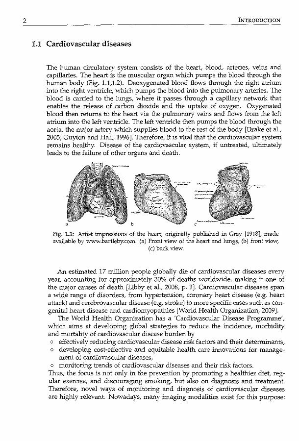
The human circulatory system consists of the heart, blood, arteries, veins and capillaries. The heart is the muscular organ which pumps the blood through the human body (Fig. 1.1,1.2). Deoxygenated blood flows through the right atrium into the right ventricle, which pumps the blood into the pulmonary arteries. The blood is carried to the lungs, where it passes through a capillary network that enables the release of carbon dioxide and the uptake of oxygen. Oxygenated blood then returns to the heart via the pulmonary veins and flows from the left atrium into the left ventricle. The left ventricle then pumps the blood through the aorta, the major artery which supplies blood to the rest of the body [Drake et a!., 2005; Guyton and Halt 1996]. Therefore, it is vital that the cardiovascular system remains healthy. Disease of the cardiovascular system, if untreated, ultimately leads to the failure of other organs and death.

Fig. 1.1: Artist impressions of the heart, originally published in Gray [1918], made available by www.bartleby.com. (a) Front view of the heart and lungs, (b) front view,

(c) back view.

An estimated 17 million people globally die of cardiovascular diseases every year, accounting for approximately 30% of deaths worldwide, making it one of the major causes of death [Libby eta!., 2008, p. 1]. Cardiovascular diseases span a wide range of disorders, from hypertension, coronary heart disease (e.g. heart attack) and cerebrovascular disease (e.g. stroke) to more specific cases such as con­genital heart disease and cardiomyopathies [World Health Organization, 2009].

The World Health Organization has a 'Cardiovascular Disease Progranune', which aims at developing global strategies to reduce the incidence, morbidity and mortality of cardiovascular disease burden by o effectively reducing cardiovascular disease risk factors and their determinants, o developing cost-effective and equitable health care innovations for manage-

ment of cardiovascular diseases, o monitoring trends of cardiovascular diseases and their risk factors.

Thus, the focus is not only in the prevention by promoting a healthier diet reg­ular exercise, and discouraging smoking, but also on diagnosis and treatment. Therefore, novel ways of monitoring and diagnosis of cardiovascular diseases are highly relevant. Nowadays, many imaging modalities exist for this purpose:

1.2 MEDICAL ULTRASOUND

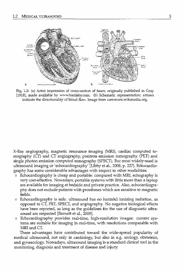
Fig. 1.2: (a) Artist impression of cross-section of heart/ originally published in Gray [1918], made available by www.bartleby.com. (b) Schematic representation; arrows

indicate the directionality of blood flow. Image from commons.wikimedia.org.

X-Ray angiography, magnetic resonance imaging (MRI), cardiac computed to­mography (CT) and CT angiography, positron emission tomography (PET) and single photon emission computed tomography (SPECT). But most widely-used is ultrasound imaging or 'echocardiography' [Libby eta!., 2008, p. 227]. Echocardio­graphy has some considerable advantages with respect to other modalities: o Echocardiography is cheap and portable: compared with MRI, echography is

very cost-effective. Nowadays, portable systems with little more than a laptop are available for imaging at bedside and private practice. Also, echocardiogra­phy does not exclude patients with prostheses which are sensitive to magnetic fields.

o Echocardiography is safe: ultrasound has no harmful ionizing radiation, as opposed to CT, PET, SPECT, and angiography. No negative biological effects have been reported, as long as the guidelines for the use of diagnostic ultra­sound are respected [Barnett eta!., 2000].

o Echocardiography provides real-time, high-resolution images: current sys­tems are suitable for imaging in real-time, with resolutions comparable with MRiandCT. These advantages have contributed toward the wide-spread popularity of

medical ultrasound, not only in cardiology, but also in e.g. urology, obstetrics, and gynaecology. Nowadays, ultrasound imaging is a standard clinical tool in the monitoring, diagnosis and treatment of disease and injury.

3

4 OORODUCTION

1.2 Medical ultrasound

1.2.1 Physics of sound

Sound is basically mechanical energy which is transmitted through a solid, liquid, or gas. Most people relate the word 'sound' to audible waves, in the form of mu­sic, verbal speech, or general noise. But in nature, sound has other uses as well. A famous example is that of the bat which uses high frequency sound waves to form an image of its surroundings. For some decades now, this principle has been put to use in the medical field to visualize objects inside the human body. Ultrasound imaging of an unborn fetus is perhaps one of the most famous exam­ples of medical ultrasound. However, ultrasound can also be used in other areas, e.g. in urology, gastroenterology, and cardiology, for monitoring and diagnosis of disease.

Diagnostic ultrasound imaging is based on the transmission and reception of high frequency sound waves. A sound wave is transmitted, which propagates through the body until it is scattered, reflected or absorbed. Part of these scat­tered and reflected waves, or echoes, are received and processed. The time be­tween transmission and reception is directly related to the distance between the source and the reflecting object and the speed of sound. Since the average ultra­sound speed through biological soft tissue can be considered as a constant value of approximately 1540 m/s, one can approximate the distance between the source and the object. Since the amount of scattered and reflected waves depends on the acoustic properties of the various media through which the ultrasound beam passes, one can make an~ acoustic' image of the :interrogated region by converting this temporal echo signal into a 'spatial' signal. For example, bone produces high echoes compared with soft tissue. By sending sound waves repeatedly, image se­quences can be obtained, allowing the analysis of temporal behavior of anatomical structures.

The propagation of an acoustic wave can be characterized by its speed c, fre­quency f, and wavelength A. This is captured in a simple relation:

c=JA. (1.1)

1n medical ultrasound, commonly used frequencies are in the range of 1 to 50 MHz, far beyond the upper limit of human hearing. The choice of frequency is a trade-off between the axial resolution and imaged depth. By increasing the frequency, higher axial resolution can be obtained. However, higher frequencies also suffer from an increased attenuation (absorption) of the ultrasound wave, resulting in a smaller penetration depth. Typically for adult echocardiography transmit frequencies of 2-4 MHz are used, which allows a penetration depth of 10-15 em.

Since a sound wave travels at a finite speed through the medium, an infinitely high frame rate cannot be achieved. The transducer has to wait for the echo to return before the next pulse is transmitted. This poses limitations on the spatial extent and frame rate of the image sequence.

1.2 MEDICAL ULTRASOUND

Image acquisition 1.2.2

Ultrasound imaging technology began with the discovery of piezo-electric mate­rials. These materials can convert an electric field into mechanical deformation and vice versa, which makes them very suitable for transmitting and receiving ultrasound waves (which is basically a mechanical deformation). Piezo-electric materials are used for the fabrication of the device used to transmit and receive ultrasound waves, the transducer.

In clinical practice, the transducer is connected to an ultrasound machine, which contains the necessary electronics to adequately process the received elec­tronic signals into images. Images are usually made by clinical experts known as sonographers, who are specially trained for this purpose. The sonographer places the transducer on the patient's body, and locates the object to be imaged by rotating and translating the transducer while watching the real-time images on a display. Images can be recorded and stored for offline analysis if desired. Nowadays, this is done digitally.

Multi-dimensional imaging 1.2.3

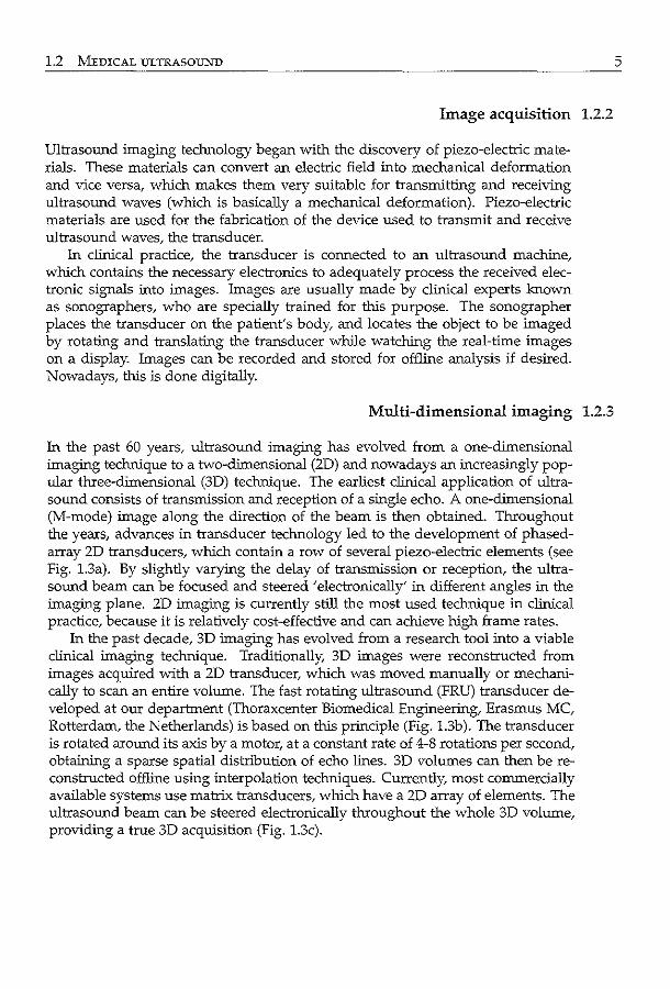
In the past 60 years, ultrasound imaging has evolved from a one-dimensional imaging technique to a two-dimensional (2D) and nowadays an increasingly pop­ular three-dimensional (3D) technique. The earliest clinical application of ultra­sound consists of transmission and reception of a single echo. A one-dimensional (M-mode) image along the direction of the beam is then obtained. Throughout the years, advances in transducer technology led to the development of phased­array 2D transducers, which contain a row of several piezo-electric elements (see Fig. 1.3a). By slightly varying the delay of transmission or reception, the ultra­sound beam can be focused and steered 'electronically' in different angles in the imaging plane. 2D imaging is currently still the most used technique in clinical practice, because it is relatively cost-effective and can achieve high frame rates.

In the past decade, 3D imaging has evolved from a research tool into a viable clinical imaging technique. Traditionally, 3D images were reconstructed from images acquired with a 2D transducer, which was moved manually or mechani­cally to scan an entire volume. The fast rotating ultrasound (FRU) transducer de­veloped at our department (Thoraxcenter Biomedical Engineering, Erasmus MC, Rotterdam, the Netherlands) is based on this principle (Fig. 1.3b). The transducer is rotated around its axis by a motor, at a constant rate of 4-8 rotations per second, obtaining a sparse spatial distribution of echo lines. 3D volumes can then be re­constructed offline using interpolation techniques. Currently, most commercially available systems use matrix transducers, which have a 2D array of elements. The ultrasound beam can be steered electronically throughout the whole 3D volume, providing a true 3D acquisition (Fig. 1.3c).

5

6 INTRODUCTION

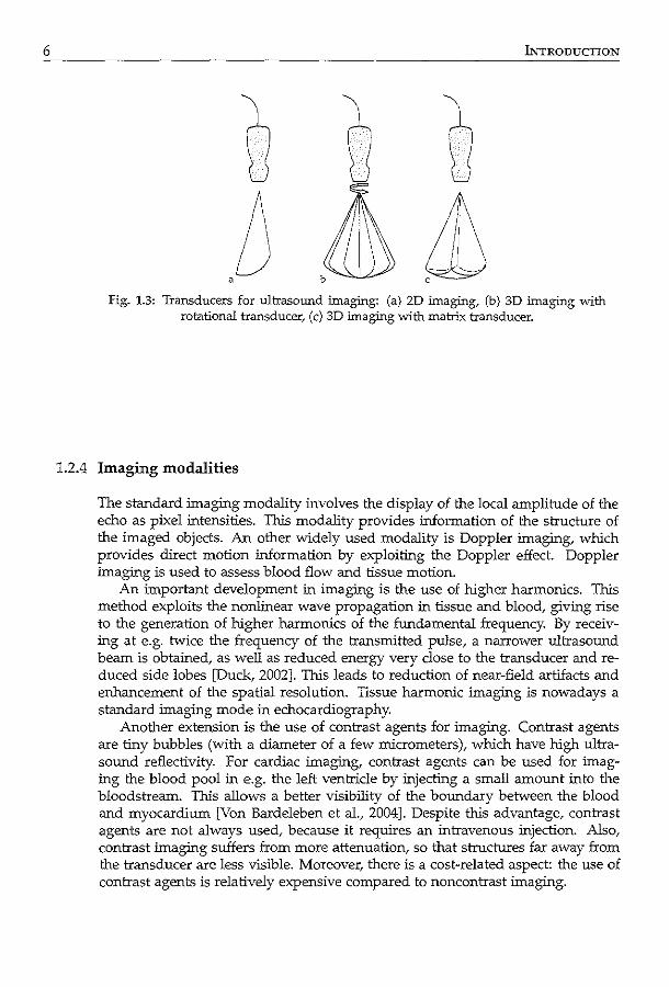
fig. 1.3: Transducers for ultrasound imaging: (a) 2D imaging, (b) 3D imaging with rotational transducer, (c) 3D imaging with matrix transducer.

1.2.4 Imaging modalities

The standard imaging modality involves the display of the local amplitude of the echo as pixel intensities. This modality provides information of the structure of the imaged objects. An other widely used modality is Doppler imaging, which provides direct motion information by exploiting the Doppler effect. Doppler imaging is used to assess blood flow and tissue motion.

An important development in imaging is the use of higher harmonics. This method exploits the nonlinear wave propagation in tissue and blood, giving rise to the generation of higher harmonics of the fundamental frequency. By receiv­ing at e.g. twice the frequency of the transmitted pulse, a narrower ultrasound beam is obtained, as well as reduced energy very close to the transducer and re­duced side lobes [Duck, 2002]. This leads to reduction of near-field artifacts and enhancement of the spatial resolution. Tissue harmonic imaging is nowadays a standard imaging mode in echocardiography.

Another extension is the use of contrast agents for imaging. Contrast agents are tiny bubbles (with a diameter of a few micrometers), which have high ultra­sound reflectivity. For cardiac imaging, contrast agents can be used for imag­ing the blood pool in e.g. the left ventricle by injecting a small amount into the bloodstream. This allows a better visibility of the boundary between the blood and myocardium [Von Bardeleben et a!., 2004]. Despite this advantage, contrast agents are not always used, because it requires an intravenous injection. Also, contrast imaging suffers from more attenuation, so that structures far away from the transducer are less visible. Moreover, there is a cost-related aspect: the use of contrast agents is relatively expensive compared to noncontrast imaging.

1.3 ECHOCARDIOGRAPHY

Echocardiography 1.3

In the previous sections, we have already touched upon the concept of echo· cardiography. Echocardiography is a cardiac imaging modality to evaluate all cardiovascular diseases related to a structural, functional, or hemodynamic ab­normality of the heart and great vessels [Libby et al., 2008, p. 277]. Ultrasound images of the heart are also known as echocardiograrns. Echocardiography is an effective tool in the diagnosis of cardiac disease, such as myocardial ischemia, congenital diseases, and valvular diseases.

Imaging 1.3.1

The most common imaging method is transthoracic imaging: the transducer is placed on the patient's chest and directed toward the heart, while avoiding the bony thoracic cage and adjacent air-filled lungs. Due to these obstacles in imag­ing, patient positioning and sonographer experience are critical factors in obtain­ing diagnostic images. Transthoracic images are typically obtained by positioning the transducer on various places on the chest, so that the heart is imaged from different angles or acoustic windows, such as the parasternal, apical, subcostal, and suprasternal notch windows ([Feigenbaum et al., 2005, p. 109], [Henry et al., 1980]).

Echocardiography can be used to image structures in the heart such as the ventricles, atria, and valves. There has been much continuing research on the left ventricle. Since oxygenated blood is pumped through the body by the left ventricle, it is important to study its structural and functional behavior. Also, by studying the motion of the left ventricle, one can deduce the health of the major coronary arteries, which supply blood to the heart itself.

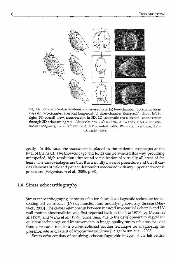
Standard tomographic planes for imaging the left ventricle are usually defined with respect to the long-axis of the left ventricle, defined as the line through the left ventricular apex and the center of the left ventricular base. Common imaging planes are, according to the current standardization for cardiac CT, cardiac MR, PET, SPECT, and echocardiography [Cerqueira et al., 2002; Otto, 2004]: o horizontal long-axis plane (approximated by the four-chamber plane in echo­

cardiography), passing through the long-axis and intersecting right and left ventricles and atria (Fig. 1.4a),

o vertical long-axis plane (approximated by the two-chamber plane in echocar­diography), passing through the long-axis, perpendicular to the horizontal long-axis plane, showing only the left ventricle and left atrium (Fig. 1.4b),

o long-axis plane (the three-chamber plane in echocardiography), passing through the long-axis and the center of the aortic valve (Fig. 1.4c),

o short-axis planes, perpendicular to the long-axis, at basal, mid-cavity, and apical heights (which should each be one-third of the long-axis) (Fig. 1.5).

These planes are the most commonly used cross-sectional images for assessing myocardial motion [Nanda et al., 2004].

Instead of transthoracic imaging, images can also be acquired transesopha-

7

8 OORODUCTION

Fig. 1.4: Standard cardiac anatomical cross-sections: (a) four-chamber (horizontal long­axis) (b) two-chamber (vertical long-axis) (c) three-chamber (long-axis). From left to right: 3D overall view, cross-section in 3D, 2D schematic cross-section, cross-section through 3D echocardiogram. Abbreviations: AO = aorta, AP = apex, LAX = left ven­tricular long-axis, LV = left ventricle, MV = mitral valve, RV = right ventricle, TV =

tricuspid valve.

geally. In this case, the transducer is placed in the patient's esophagus at the level of the heart. The thoracic cage and lungs can be avoided this way, providing unimpeded, high resolution ultrasound visualization of virtually all areas of the heart. The disadvantages are that it is a mildly invasive procedure and that it car­ries elements of risk and patient discomfort associated with any upper endoscopic procedure [Feigenbaum eta!., 2005, p. 60].

1.4 Stress echocardiography

Stress echocardiography, or stress echo for short, is a diagnostic technique for as­sessing left ventricular (LV) dysfunction and underlying coronary disease [Mar­wick, 2003]. The causal relationship between induced myocardial ischemia and LV wall motion abnormalities was first reported back in the late 1970's by Mason et a!. [1979] and Warm eta!. [1979]. Since then, due to the development in digital ac­quisition technology and improvements in image quality, stress echo has evolved from a research tool to a well-established routine technique for diagnosing the presence, site and extent of myocardial ischemia [Feigenbaum eta!., 2005].

Stress echo consists of acquiring echocardiographic images of the left ventri-

1.4 STRESS ECHOCARDIOGRAPHY

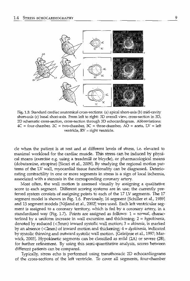
Fig. 1.5: Standard cardiac anatomical cross-sections: (a) apical short-axis (b) mid-cavity short-axis (c) basal short-axis. From left to right 3D overall view/ cross-section in 3D, 2D schematic cross-section, cross-section through 3D echocardiogram. Abbreviations: 4C = four-chamber, 2C = two-chamber, 3C = three-chamber, AO = aorta, LV = left

ventricle, RV = right ventricle.

de when the patient is at rest and at different levels of stress, i.e. elevated to maxilnal workload for the cardiac muscle. This stress can be induced by physi­cal means (exercise e.g. using a treadmill or bicycle), or pharmacological means (dobutamine, atropine) [Sicari et al., 2009]. By studying the regional motion pat­terns of the LV wall, myocardial tissue functionality can be diagnosed. Deterio­rating contractility in one or more segments in stress is a sign of local ischemia, associated with a stenosis in the corresponding coronary artery.

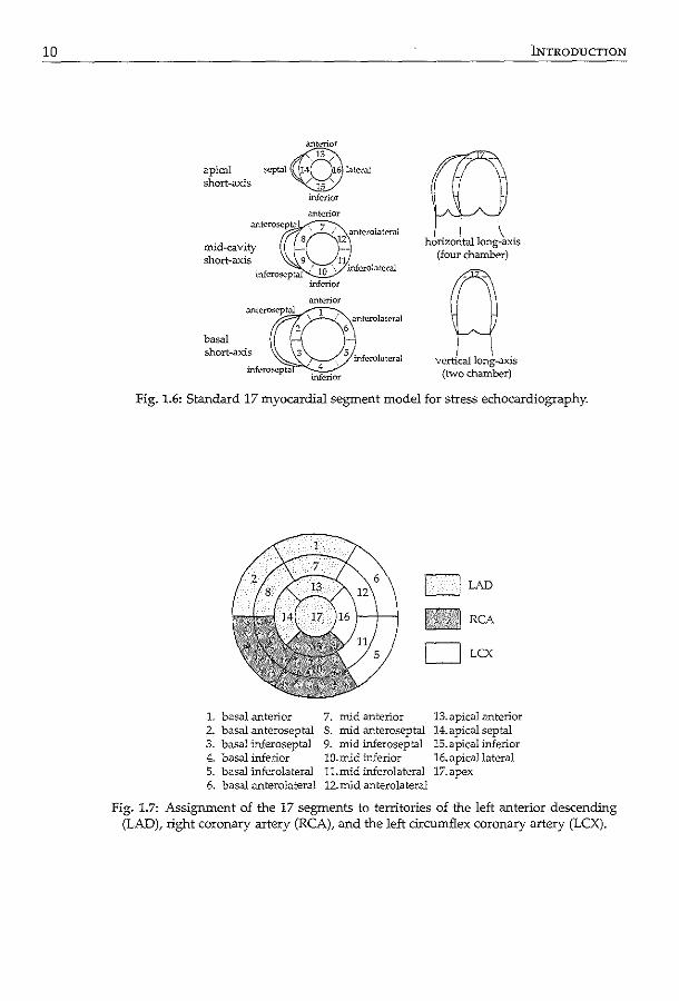
Most often, the wall motion is assessed visually by assigning a qualitative score to each segment. Different scoring systems are in use; the currently pre­ferred system consists of assigning points to each of the 17 LV segments. The 17 segment model is shown in Fig. 1.6. Previously, 16 segment [Schiller et al., 1989] and 13 segment models [Nijland et al., 2002] were used. Each left ventricular seg­ment is assigned to a coronary territory, which is fed by a coronary artery, in a standardized way (Fig. 1.7). Points are assigned as follows: 1 = normal, charac­terized by a uniform increase in wall excursion and thickening; 2 = hypokinesia, denoted by reduced ( <5mm) inward systolic wall motion; 3 = akinesia, is marked by an absence ( <2mm) of inward motion and thickening; 4 = dyskinesia, indicated by systolic thinning and outward systolic wall motion. [Geleijnse et al., 1997; Mar­wick, 2003]. Hypokinetic segments can be classified as mild (2A) or severe (2B), for further refinement. By using this semi-quantitative analysis, scores between different patients can be compared.

Typically, stress echo is performed using transthoracic 2D echocardiograms of the cross-sections of the left ventricle. To cover all segments, four-chamber

9

10

apical ~

short-axis

basal short-axis

inferior

.mtcrior

inferior

(Q horizontal long-axis

(four chamber)

q vertical long-axis

(two chamber)

INTRODUCTION

Fig. 1.6: Standard 17 myocardial segment model for stress echocardiography.

DLAD

RCA

OLcx

1. basal .anterior 7. mid anterior 13. apical anterior 2. basal anteroseptal 8. mid anteroseptal 14.apical septal 3. basal inferoseptal 9. mid inferoseptal 15.apical inferior 4. basal inferior lO.mid inferior 16.apicallateral 5. basal inferolateral ll.mid inferolateral 17.apex 6. basal anterolateral 12.mid anterolateral

Fig. 1.7: Assignment of the 17 segments to territories of the left anterior descending (LAD), right coronary artery (RCA), and the left circumflex coronary artery (LCX).

1.4 STRESS ECHOCARDIOGRAPHY

and two-chamber views are acquired from the apical window, and long-axis and short-axis views from the parasternal window. For exercise stress, images are usually acquired in the rest and peak (or immediately after) exercise [Feigenbaum eta!., 2005, p. 491-3]. For dobutamine stress, rest, low-dose, peak and recovery stages are recorded [Geleijnse eta!., 1997]. Contrast can be applied to enhance the myocardial wall visibility in patients who are difficult to image. To facilitate wall motion analysis, images of the various stages can be displayed next to each other in one screen (for the standard dobutamine stress, this is called the quadscreen format).

Although widely applied, 2D stress echo is not void of some limitations: o variabilities in imaged cross-sections: the acquisition of stress echo images

is complex and requires elaborate protocols. To find the optimal 2D cross­sections, the sonographer has to translate and rotate the ultrasound probe in the right position. This is especially challenging in the stress stage, as only a limited time span is available for the acquisition. Related to this is the problem of the foreshortening of apical views: the actual imaged 4-chamber, 2-chamber, and long-axis cross-sections may not pass through the long-axis at all, because ribs or other obstructions frequently force the sonographer to choose suboptimal cross-sections. This is especially problematic in the analy­sis of apical segments.

o variabilities in interpretation: since the wall motion scores are assigned vi­sually, interpretations may differ between two institutions, between two ob­servers, or even within one observer analyzing at different times [Hoffmann et a!., 1996, 2002]. Subtle differences between normal and abnormal motion, un­der varying circumstances and cross-sections, may be hard to judge visually. This is widely acknowledged as a major weakness of stress echo.

Therefore, both stress echo acquisition as well as interpretation require a long learning curve.

Recently, there has been much interest in 3D stress echo [Armstrong and Zoghbi, 2005; Matsumura et a!., 2005; Yang et a!., 2006; Zwas et al., 1999]. Re­cent advances in real-time 3D echocardiography [Caiani eta!., 2005; Jenkins eta!., 2006], show great potential in overcoming the major limitations of traditional 2D stress echocardiography [Lang et al., 2006b; Monaghan, 2006]: o better standardization of cross-sections: since 3D echo can image the whole

left ventricle, optimal 2D cross-sections can be selected retrospectively for vi­sual analysis. This can be done manually by following more consistent pro­tocols, or the whole process can be automated. Also, since the whole LV is imaged at the same time, the acquisition is greatly simplified. This is espe­cially relevant in the stress acquisition.

o quantification of true 3D wall motion: since the heart is a 3D structure, with 3D echo, the true 3D behavior of the heart can be analyzed. 3D echo allows by definition more accurate, realistic, and detailed volume and motion analysis, simply because more image information is available. However, real-time 3D echocardiography for stress testing currently still poses

some challenges, compared with 2D imaging: o limited spatiotemporal resolution: as discussed earlier in section 1.2.1, the

11

12 INTRODUCTION

finite speed of sound limits the spatial extent and frame rate of the image sequence. Every extra scan plane that is acquired in the third dimension re­duces the maximum frame rate. Because of this limitation, full volume imag­ing of the left ventricle is currently achieved by stitching four to seven smaller subvolumes, each acquired from a single heartbeat [Von Bardeleben et a!., 2004]. If the position of the heart or the transducer changes during this time, it may lead to motion artifacts, which present themselves as discontinuities from one subvolume to the next [Brekke et a!., 2007; Yang et al., 2008a]. Cur­rently, it is therefore recommended that a small scan sector is chosen. Lately, clever ultrasound beamforming technologies have been investigated to reduce the imaging time to a single cardiac cycle, thus shortening the acquisition time and eliminate stitching artifacts [Lang et a!., 2006b]. Last year, two of the major manufacturers launched such ultrasound systems (Siemens: ACUSON SC2000, GE: Vivid E9). The image quality obtained using these promising systems remains a subject of future research.

o technological challenges: current commercial systems make use of matrix ar­ray transducers, which typically have a larger surface area than a 2D trans­ducer. This makes it more difficult to image between the ribs, often resulting in suboptimal imaging of parts of the myocardium. Also, the fact that the signal from each of approximately 2000 piezo-electric element needs to be analyzed, makes it especially challenging from an electronics point-of-view. Also, measures may have to be taken to prevent overheating of the electronics.

o image rendering and clinical workflow challenges: despite the fact that a 3D image is made, 2D cross-sections are usually used for stress analysis, since current displays merely render the image in 2D. Systematic methods for se­lecting the correct anatomical views are therefore necessary. If this takes too much time, it will adversely affect the clinical workflow of stress echo.

o challenges in automated image analysis: the wealth of data in 3D may ulti­mately require smart automated methods for quantification of left ventricular clinical parameters [Badano et al., 2007; Hung et a!., 2007]. For example, to calculate the true 3D volume of the left ventricle, the endocardial border must be delineated in 3D. Obviously, this is very difficult and labor intensive to do manually. Therefore, besides the challenges in transducer design [Von Bardeleben et a!.,

2004], it becomes apparent that the development of automatic methods for classi­fying wall-motion, which emulate visual wall motion scoring, is highly desirable.

1.5 Automated analysis of ultrasound images

1.5.1 Automated analysis

In this thesis, we describe some computerized, or automated, methods for ana­lyzing ultrasound images. The field of image processing, which encompasses the

1.5 AUTOMATED ANALYSIS OF ULTRASOUND IMAGES

development of such automated methods, can be described as 'the manipulation and analysis of information contained in images' [Maintz, 2005]. This is of course a very broad definition, and image processing has applications in may research areas, such as forensic science (e.g. video surveillance, fingerprint analysis, DNA coding), industry (e.g. checking of manufactured parts), and information process­ing (e.g. recognition of handwritten text, scanning and classification of printed images). By developing automated methods, we aim to emulate what a human observer would do, by teaching the computer to do the same.

From the study of human perception, we know that vision is all but a simple, straightforward process. The interpretation of highly complex information like ultrasound images is a very complicated process, using both 'low' and 'high' abstraction levels. A common analogy is in the example of written text: the interpretation is performed at low to high levels, from alphabet and spelling, to vocabulary, syntax, and semantics, ultimately to the subject of the text and adornments like humor, sarcasm, and metaphors. For image analysis, this is generally known as the image interpretation pyramid [Otto, 2007, p. 266].

Given the difficulties in ultrasound image interpretation, one can envision that the incorporation of prior knowledge may be beneficial in developing automated analysis methods [Noble and Boukerroui, 2006]. Prior knowledge can manifest itself as image features, such as assumptions on the image intensity distribution (e.g. Rayleigh distribution), intensity gradients and higher derivatives, phase, and texture. Prior knowledge on shape is particularly useful in ultrasound images, due to the presence of attenuation, shadowing artifacts, and speckle. Temporal priors or models are also relevant in ultrasound imaging, since it is a real-time modality. Visual inspection of an ultrasound image sequence is easier than the analysis of a still frame.

In this thesis, many methods exploit prior knowledge in the form of math­ematical models. These models may contain information on the left ventricular structure (shape), function (motion), or appearance (what the heart looks like in the ultrasound images). More specifically, they describe typical values and varia­tions across many patients, which are gathered using expert observer knowledge. In other words, the models are trained using observer data. The model can then be used to estimate the model variation which best fits an image of a new patient, a process called matching. These models operate on the higher abstraction levels of the interpretation pyramid.

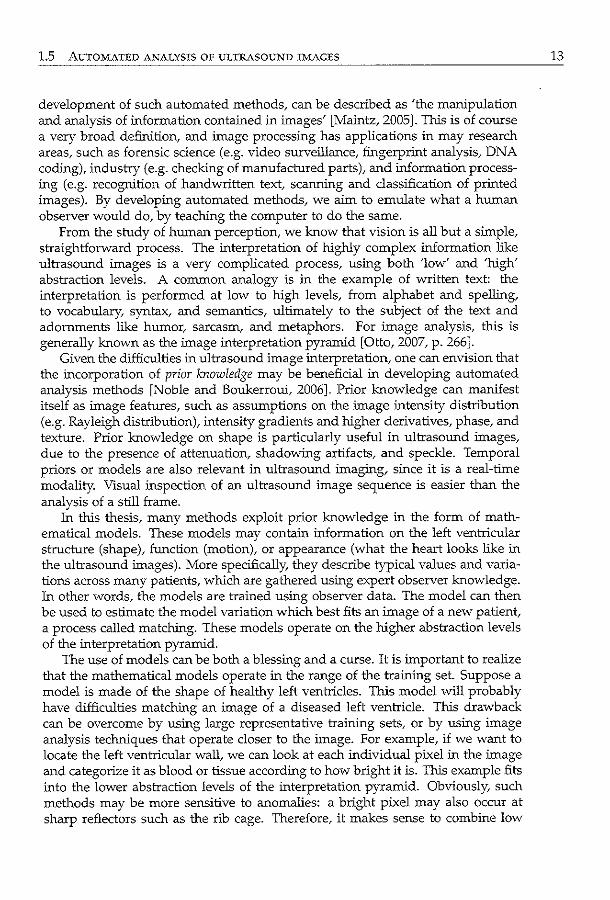
The use of models can be both a blessing and a curse. It is important to realize that the mathematical models operate in the range of the training set. Suppose a model is made of the shape of healthy left ventricles. This model will probably have difficulties matching an image of a diseased left ventricle. This drawback can be overcome by using large representative training sets, or by using image analysis techniques that operate closer to the image. For example, if we want to locate the left ventricular wall, we can look at each individual pixel in the image and categorize it as blood or tissue according to how bright it is. This example fits into the lower abstraction levels of the interpretation pyramid. Obviously, such methods may be more sensitive to anomalies: a bright pixel may also occur at sharp reflectors such as the rib cage. Therefore, it makes sense to combine low

13

14 INTRODUCTION

and high levels of abstraction in the analysis methods.

1.5.2 Requirements for automated methods for stress echo

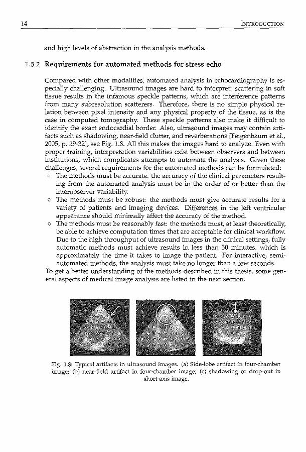
Compared with other modalities, automated analysis in echocardiography is es­pecially challenging. Ultrasound images are hard to interpret: scattering in soft tissue results in the infamous speckle patterns, which are interference patterns from many subresolution scatterers. Therefore, there is no simple physical re­lation between pixel intensity and any physical property of the tissue, as is the case in computed tomography. These speckle patterns also make it difficult to identify the exact endocardial border. Also, ultrasound images may contain arti­facts such as shadowing, near-field clutter, and reverberations [Feigenbaum et a!., 2005, p. 29-32], see Fig. 1.8. All this makes the images hard to analyze. Even with proper training, interpretation variabilities exist between observers and between institutions, which complicates attempts to automate the analysis. Given these challenges, several requirements for the automated methods can be formulated: o The methods must be accurate: the accuracy of the clinical parameters result­

ing from the automated analysis must be in the order of or better than the interobserver variability.

o The methods must be robust: the methods must give accurate results for a variety of patients and imaging devices. Differences in the left ventricular appearance should minimally affect the accuracy of the method.

o The methods must be reasonably fast: the methods must, at least theoretically, be able to achieve computation times that are acceptable for clinical workflow. Due to the high throughput of ultrasound images in the clinical settings, fully automatic methods must achieve results in less than 30 minutes, which is approximately the time it takes to image the patient. For interactive, semi­automated methods, the analysis must take no longer than a few seconds.

To get a better understanding of the methods described in this thesis, some gen­era! aspects of medical image analysis are listed in the next section.

Fig. 1.8: Typical artifacts :in ultrasound images. (a) Side-lobe artifact in four-chamber image; (b) near-field artifact ill four-chamber image; (c) shadowing or drop-out in

short-axis image.

1.6 METHODS FOR MEDICAL IMAGE ANALYSIS

Methods for medical image analysis 1.6

Medical image analysis is an active field of research worldwide. Many researchers work on a vast variety of automated analysis methods for modalities such as MRI, CT, PET, SPECT, and ultrasound, for the imaging of many organs and for the diagnosis of many kinds of diseases. For ultrasound, much effort has been put into cardiovascular applications: the analysis of the heart, the coronary arteries, the carotid arteries, and aorta, to study the cardiovascular anatomy and function.

In this large variety of automated analysis methods, one can distinguish some important directions of research, which are described below. Here, we strive to give a global overview of methods which are used in a medical context, without going into the details of individual methods. It is important to note that many analysis methods make use of more than one of these research directions. For a more detailed description, we refer to recent reviews in the literature and to the individual introductions in the following thesis chapters.

15

Image filtering 1.6.1

Image filtering is often applied for preparing the images for further analysis. This process modifies the intensity values of the images, either to enhance interesting parts of the image (such as edges), or to reduce noise, for optimal visual and quantitative analysis. A basic example is setting the brightness and contrast levels on a monitor. Such global intensity transforms affect each pixel individually: by transforming the histogram of all image intensities, new intensity values are assigned to each pixel. Other common examples of histogram operations include thresholding and all kinds of linear and nonlinear intensity mapping techniques (such as histogram equalization). Nowadays, these image enhancement methods are also available in commercial image editing software.

Another common way of enhancing images is by using neighborhood-based filters. Filters operate on regions-of-interest containing multiple pixels, via the spatial convolution of the image with a kernel, generating a new, improved im­age. These kernels operate in the neighborhood of an image pixel. For example, an averaging kernel replaces a pixel in the image with the average value in a re­gion around the pixel. This is then performed for all pixels in the image. Thus, averaging has the effect of 'smoothing' or 'blurring' the image. Other commonly used smoothing filters include median and Gaussian filtering. The disadvan­tage of such smoothing filters is that they may blur sharp boundaries that distin­guish between large anatomical structures. Anisotropic filtering tries to preserve these boundaries, while smoothing within individual anatomical structures [Per­ona and Malik, 1990]. Buades et al. [2000] gives a review of general image noise removal algorithms.

For ultrasound images, much effort has been put into techniques for reduction of local speckle patterns, thus enhancing the global interface between anatomical structures (e.g. blood/tissue boundaries). This is not a trivial problem, andre­quires more dedicated filters. Speckle reduction is an active field of research; for

16 INTRODUCTION

more advanced speckle reduction techniques, we refer to the literature (see e.g. [Sun et al., 2004; Tay et a!., 2006; Yu and Acton, 2002]).

1.6.2 Image restoration and artifact detection

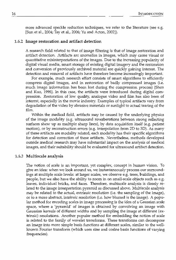
A research field related to that of image filtering is that of image restoration and artifact detection. Artifacts are anomalies in images, which may cause visual or quantitative misinterpretations of the images. Due to the increasing popularity of digital visual media, smart storage of existing digital imagery and the restoration and conversion of previously archived material are quickly gaining interest. The detection and removal of artifacts have therefore become increasingly important.

For example, much research effort consists of smart algorithms to efficiently compress digital images, and in restoration of badly compressed images (i.e. much image information has been lost during the compression process) [Shen and Kuo, 1998]. In this case, the artifacts were introduced during digital com­pression. Restoration of low quality, analogue video and film has also been of interest, especially in the movie industry. Examples of typical artifacts vary from degradation of the video by abrasive materials or sunlight to actual tearing of the film.

Within the medical field, artifacts may be caused by the underlying physics of the image modality (e.g. ultrasound reverberations between strong reflecting surfaces show up as multiple sharp lines), by data acquisition itself (e.g. patient motion), or by reconstruction errors (e.g. interpolation from 2D to 3D). As many of these artifacts are modality related, each modality has their specific algorithms for detection and correction of these artifacts. Nevertheless, methods developed outside medical research may have substantial impact on the analysis of medical images, and their suitability should be evaluated for ultrasound artifact detection.

1.6.3 Multiscale analysis

The notion of scale is an important, yet complex, concept in human vision. To give an idea: when we look around us, we instantaneously process our surround­IDgs at multiple scale levels: at larger scales, we observe e.g. trees, buildings, and people, but we also have the ability to zoom in on small-scale objects such as e.g. leaves, individual bricks, and faces. Therefore, multiscale analysis is closely re­lated to the image interpretation pyramid as discussed above. Multiscale analysis may be related to the actual, extrinsic resolution (i.e. the sampling of the image), or to a more abstract, intrinsic resolution (i.e. how blurred is the image). A popu­lar method for encoding scales in image processing is the idea of a Gaussian scale space, where a 'pyramid' of images is obtained by convolving an image with Gaussian kemels of different widths and by sampling the image at different (ex­trinsic) resolutions. Another popular method for embedding the notion of scale is related to the family of wavelet transforms. These transforms can decompose an image into more simple basis functions at different scales, similar to the well­known Fourier transform (which uses sine and cosine basis functions of varying frequencies).

1.6 METHODS FOR MEDICAL IM:AGE ANALYSIS

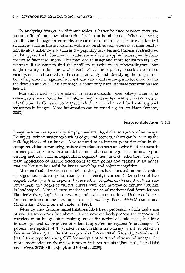
By analyzing images on different scales, a better balance between interpre­tation at 'high' and 'low' abstraction levels can be obtained. When analyzing an ultrasound image for example, at coarser resolution levels, coarse anatomical structures such as the myocardial wall may be observed, whereas at finer resolu­tion levels, smaller details such as the papillary muscles and trabecular structures can be appreciated. Commonly, multiscale analysis is applied subsequently from coarser to finer resolutions. This may lead to faster and more robust results. For example, if we want to find the papillary muscles in an echocardiogram, one might first try to find the cardiac wall. Since the papillary muscles are in this vicinity, one can then reduce the search area. By first identifying the rough loca­tion of a particular region-of-interest, one can avoid running into local minima in the detailed analysis. This approach is commonly used in image registration (see below).

More advanced uses are related to feature detection (see below). Interesting research has been conducted for determining local key features (such as corners or edges) from the Gaussian scale space, which can then be used for locating global structures in images. More information can be found e.g. in [ter Haar Romeny, 2003].

17

Feature detection 1.6.4

Image features are essentially simple, low-level, local characteristics of an image. Examples include structures such as edges and corners, which can be seen as the building blocks of an image. Also referred to as interest point detection in the computer vision community, feature detection has been an active field of research for many decades now. Feature detection is often an integral part in image pro­cessing methods such as registration, segmentation, and classification. Today, a main application of feature detection is to find points and regions in an image that are likely to be useful for image matching and object recognition.

Most methods developed throughout the years have focused on the detection of edges (i.e. sudden spatial changes in intensity), corners (intersection of two edges), blobs (points or regions that are either brighter or darker than their sur­roundings), and ridges or valleys (curves with local maxima or minima, just like in landscapes). Most of these methods make use of mathematical formulations like derivatives, Laplacian operators, and scale-space notions. Listings of detec­tors can be found in the literature, see e.g. [Lindeberg, 1993, 1998b; Mohanna and Mokhtarian, 2001; Ziou and Tabbone, 1998].

Recently, new feature representations have been proposed, which make use of wavelet transforms (see above). These new methods process the response of wavelets to an image, often making use of the notion of scale-space, resulting in more general descriptions of interesting points or regions in an image. A popular example is SIFT (scale-invariant feature transform), which is based on Gaussian filtering at different image scales [Lowe, 2004]. Recently, Moradi et a!. [2006] have reported using SIFT for analysis of MRI and ultrasound images. For more information on these new types of features, see also [Bay et a!., 2008; Dalal and Triggs, 2005; Mikolajczyk and Schmid, 2005].

18 Ll\JTRODUCTION

For finding larger-scale, parametric structures like circles and cylinders, the Hough transform [Hough, 1962] has proved to be a useful and robust detector. Although the original formulation only allowed the detection of straight lines and circles, this technique has been extended to more complex parametric structures [Ballard, 1981]. Previously, it has been used to detect cardiac structures in MRI [Miiller et al., 2005; van der Geest et al., 1997] and ultrasound images [Golemati et al., 2007; Solairnan et al., 1998].

1.6.5 Statistical modeling

Throughout the years, statistical modeling has become a popular concept for de­scribing the typical variations in the shape, appearance, and composition of the parts of the human body. In general, statistical modeling aims at deriving mathe­matical formulations which describe these typical variations. These models can be used to study variations in patient populations (e.g. differences between healthy and diseased populations). More importantly, they can be used for segmentation and registration purposes. We have already touched upon this concept in the previous section on automated analysis (section 1.5.1).

For shape modeling, point distribution models are most often used. Point distribution models characterize shape and shape variability based on Principal Component Analysis (PCA) [Cootes et al., 1992]. Shape knowledge is derived from a training set of example shapes, extracted e.g. by delineating contours in medical images. The shapes themselves are expressed in coordinates of landmark points, which are placed at consistent, identifiable locations in the images. After spatially aligning these shapes, PCA is applied, which generates a linear, mathe­matical model of a mean shape and a number of characteristic shape variations. Within certain statistical limits, shapes resembling those from the training set can be approximated using the mean shape and a linear combination of the shape variations. Inspired by Cootes' work on face modeling, point distribution models have found their way in a large variety of medical applications, modeling complex structures which have a globally distinct shape.

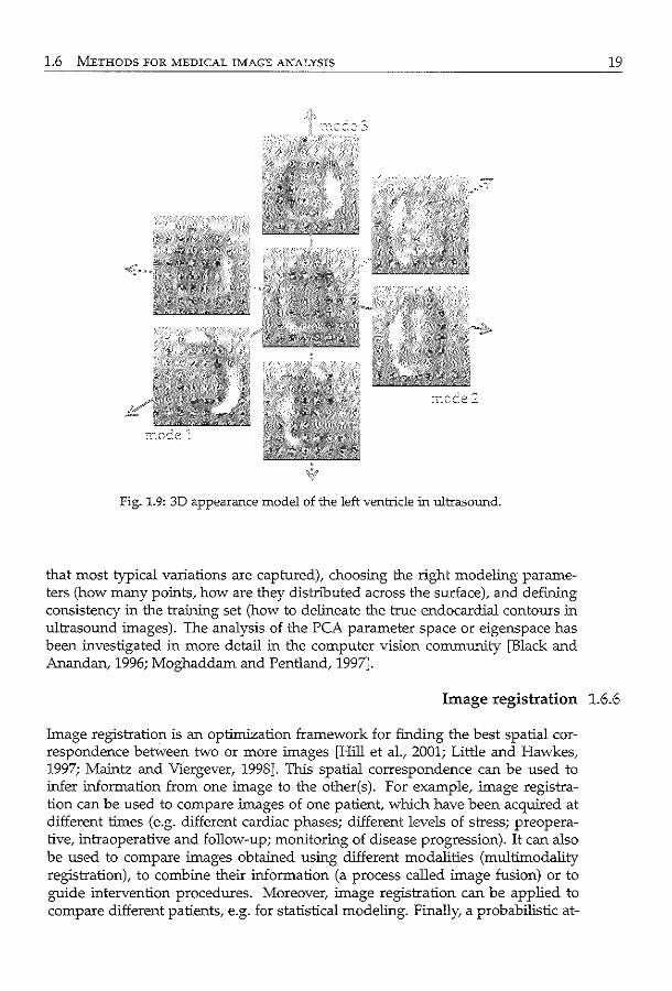
A similar concept can be used to generate models of the typical look of an image, by applying Principal Component Analysis to image intensities. To re­move size and shape dependence from these models, the images first need to be interpolated to a common coordinate frame. To satisfy the requirement of nor­mality, intensities also need to be normalized to a Gaussian distribution. The resulting model is also called a texture model. The combination of shape and texture model is the appearance model, which describes combined variations of shape and texture [Cootes et al., 2001] (see Fig. 1.9).

A common way to incorporate temporal information into these models is by putting shape or texture information from multiple time points into the same model. In this way, temporal information is modeled implicitly. This has been used e.g. in cardiac modeling [Bosch et al., 2002], as the cardiac phases are quite well defined for most patients. More recently, temporal information has been modeled separately from the spatial information, see e.g. Perperidis et al. [2007].

The challenge in creating a model involves selecting the training data (such

1.6 METHODS FOR MEDICAL IMAGE ANALYSIS

Fig. 1.9: 3D appearance model of the left ventricle in ultrasound.

that most typical variations are captured), choosing the right modeling parame­ters (how many points, how are they distributed across the surface), and defining consistency in the training set (how to delineate the true endocardial contours in ultrasound images). The analysis of the PCA parameter space or eigenspace has been investigated in more detail in the computer vision community [Black and Anandan, 1996; Moghaddam and Pentland, 1997].

19

Image registration :L6.6

lmage registration is an optimization framework for finding the best spatial cor­respondence between two or more images [Hill et al., 2001; Little and Hawkes, 1997; Maintz and Viergever, 1998]. This spatial correspondence can be used to infer information from one image to the other(s). For example, image registra­tion can be used to compare images of one patient, which have been acquired at different times (e.g. different cardiac phases; different levels of stress; preopera­tive, intraoperative and follow-up; monitoring of disease progression). It can also be used to compare images obtained using different modalities (multimodality registration), to combine their information (a process called image fusion) or to guide intervention procedures. Moreover, image registration can be applied to compare different patients, e.g. for statistical modeling. Finally, a probabilistic at-

20 INTRODUCTION

las (a pixel-based representation of an 'average' organ in the patient population) can be registered to an individual patient.

There are, roughly speaking, two main image registration methods: (1) land­mark and surface-based methods and (2) intensity-based methods. The first cat­egory aims at finding the best correspondence between landmarks or contours, which define the object of interest in images [Audette et al., 2000]. These land­marks can be physically introduced into the image space (e.g. skin markers on the patient) or extracted from the images themselves (anatomical or geometri­cal landmarks, contours of objects). The similarity between these landmarks or contours are geometrical measures, such as Euclidean distances. The intensity­based methods operate on the actual image intensities. 1n this case, the similarity between the images is a measure of correspondence. Since the intensity-based method is the most widely used, the following paragraphs mainly concentrate on this technique.

Finding the best spatial correspondence is not a trivial task. Images can differ in appearance, for example if tumor growth is present. Differences can also be more significant, especially when images of different modalities need to be com­pared. Also, there are considerable differences in anatomy between patients. An­other issue concerns the dimensionality of the data (2D, 2D+time, 3D, 3D+time): the images to be registered need not have the same dimensionality. Due to these challenges, image registration has become an important and popular subject of research in a wide variety of medical applications [Pluim and Fitzpatrick, 2003].

The spatial correspondence is encoded in a spatial transform between the two images. When registering two images, one is often denoted as the 'fixed' or 'ref­erence' image, and the other image on which the spatial transform is applied is denoted as the 'moving' image. Depending on the desired degree of align­ment, this spatial transform can be rigid, affine, projective, or curved [Maintz and Viergever, 1998]. A rigid transformation consists of only translations and rota­tions. Affine transforms also include scaling and shearing, but still map parallel lines in one image onto parallel lines in the other image. A step further is the projective transformation, which maps lines onto lines. Finally, if the transform maps lines onto curves, it is called curved or elastic. A transform is represented by a set of parameters; the number of parameters increases with the complexity of the transform. A transformation is called global if it applies to the entire im­age, and local if subsections of the image each have their own transformations defined. The term nonrigid registration is generally used to indicate all types of transforms besides the global rigid transformation, although some consider also (global) affine transforms to be rigid.

The similarity criterion, or metric.r is a measure of correspondence for intensi­ty-based registration. Some basic metrics are the sum-of-absolute differences in intensity between the two images, the sum-of-squared differences, and the cross­correlation metric. These are commonly used for registering images of the same modality. 1n the past two decades, the mutual information metric has become popular [Pluim et al., 2003]. Mutual information, based on Shannon's information entropy, measures the mutual dependency of two random variables (in this case, images) X and Y. Simply put, it is a measure that expresses with what certainty

1.6 METHODS FOR MEDICAL IMAGE ANALYSIS

does one know Y, given that one knows X. Muhlal information is computed using estimates of probability distributions of the images and their joint distribution. Since this metric only assumes that each intensity value in image X has a single counterpart in image Y (and vice versa), it is very suitable for multimodality registration.

Given the complexity of these transforms, one can imagine that a brute-force search over the entire parameter space to find the best spatial correspondence is almost impossible. Registration is basically an iterative optimization framework for finding this spatial correspondence in a smart way, without exhaustively eval­uating the entire parameter space. During each iteration, the current estimate of the spatial transform is applied to the moving image. The metric is calculated and passed on to an optimizer, which generates a new estimation of the spatial transform. The process is repeated until the images are sufficiently aligned. Opti­mizers may rely on the computation of gradients (gradient ascent, quasi-Newton methods, Levenberg-Marquardt); other routines do not use gradient information (Powell, Simplex) [Pluim eta!., 2003]. Many optimizers stem from general math­ematical optimization research [Press eta!., 1992].

The spatial transform is actually applied to the coordinates of the moving image, after which the intensity values are resampled from the moving image. In many cases an interpolation step is required, since the coordinates often do not match the image grid exactly. Again, many variants exist, most commonly used are nearest neighbor, linear, and b-spline interpolation [Hill eta!., 2001]. For mutual information, partial volume interpolation is often recommended [Pluim eta!., 2003].

Due to the nature of the optimization framework, the starting estimates of the spatial transform need to be sufficiently close to the correct position. Otherwise, the optimization may run into local minima in the parameter space. A common way to limit this is to use registration in coarse to fine image resolutions, again exploiting the multiscale paradigm [Lester and Arridge, 1998]. Also, the number of parameters to optimize can be expanded tluough each scale, e.g. a nonrigid registration is performed after initialization by rigid registration.

21

Motion analysis 1.6.7

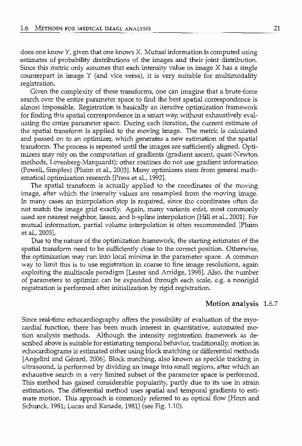
Since real-time echocardiography offers the possibility of evaluation of the myo­cardial function, there has been much interest in quantitative, automated mo­tion analysis methods. Although the intensity registration framework as de­scribed above is suitable for estimating temporal behavior, traditionally, motion in echocardiograrns is estimated either using block matching or differential methods [Angelini and Gerard, 2006]. Block matching, also known as speckle tracking in ultrasound, is performed by dividing an image into small regions, after which an exhaustive search in a very limited subset of the parameter space is performed. This method has gained considerable popularity, partly due to its use in strain estimation. The differential method uses spatial and temporal gradients to esti­mate motion. This approach is commonly referred to as optical flow [Hom and Schunck, 1981; Lucas and Kanade, 1981] (see Fig. 1.10).

22 INTRODUCTION

Fig. 1.10: Example of motion vector field in short-axis image, computed using optical flow tracking.

Other considerable research effort focuses on using model prediction and state estimation methods, such as Kalman techniques Uacob et al., 2002, 1999; Orderud et al., 2007b]. The Kalman filter is a recursive filter that estimates the underlying parameters of a dynamic system from a series of incomplete and noisy measure­ments [Maybeck, 1979]. More advanced filters, such as particle filters [Arulam­palam eta!., 2002t are becoming increasingly popular. Expectation-maximization [Dempster eta!., 1977t which is used for finding maximum likelihood estimates of parameters in probabilistic models, has also been applied [Lorenzo-Valdes et a!., 2004]. Another example is the concept of information fusion, which was ap­plied by Comaniciu et al. [2004] for combining noisy motion estimates with sta­tistical models.

1.6.8 Segmentation

Segmentation, in its broadest sense, is the division of an image into meaningful, nonoverlapping regions. These regions correspond with objects or areas of the real world contained in the image. It has been a key focus of research in the field of medical image analysis. A myriad of methods have been proposed; however, in spite of the huge effort invested, there is no single approach that can generally solve the problem of segmentation for the large variety of image modalities and applications existing today. An excellent review on ultrasound image segmenta­tion is provided by Noble and Boukerroui [2006].

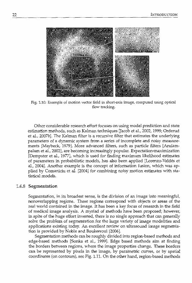
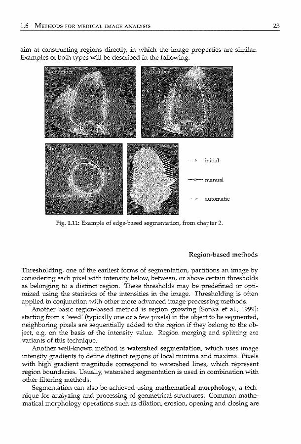
Segmentation methods can be roughly divided into region-based methods and edge-based methods [Sonka et al., 1999]. Edge based methods aim at finding the borders between regions, where the image properties change. These borders can be represented by pixels in the image, by parametric curves, or by spatial coordinates (on contours), see Fig. 1.11. On the other hand, region-based methods

1.6 METHODS FOR MEDICAL IMAGE ANALYSIS

aim at constructing regions directly, in which the image properties are similar. Examples of both types will be described in the following.

initial

-;:-manual

automatic

Fig. 1.11: Example of edge-based segmentation, from chapter 2.

Region-based methods

Thresholding, one of the earliest forms of segmentation, partitions an image by considering each pixel with intensity below, between, or above certain thresholds as belonging to a distinct region. These thresholds may be predefined or opti­mized using the statistics of the intensities in the image. Thresholding is often applied in conjunction with other more advanced image processing methods.

Another basic region-based method is region growing [Sonka et a!., 1999]: starting from a 'seed' (typically one or a few pixels) in the object to be segmented, neighboring pixels are sequentially added to the region if they belong to the ob­ject, e.g. on the basis of the intensity value. Region merging and splitting are variants of this tecl:uUque.

Another well-known method is watershed segmentation, which uses image intensity gradients to define distinct regions of local minima and maxima. Pixels with high gradient magnitude correspond to watershed lines, which represent region boundaries. Usually, watershed segmentation is used in combination with other filtering methods.

Segmentation can also be achieved using mathematical morphology, a tech­nique for analyzing and processing of geometrical structures. Common mathe­matical morphology operations such as dilation, erosion, opening and closing are

23

24 INTRODUCTION

based on topological and geometrical concepts such as size, shape, and connec­tivity. Mathematical morphology can also be used for image noise reduction and enhancement of object structure (e.g. thinning of edges).

Classification methods can be used to label pixels as corresponding with sep­arate regions (see section 1.6.9 for more details). The features are extracted from the image, e.g. using the techniques in section 1.6.4. The methods can be unsu­pervised or supervised. Neural networks have been particularly popular in this type of ultrasound image segmentation.

Graph partitioning methods can also be used for image segmentation. The image is represented as a graph, in which each pixel is a node. An link is formed between every pair of pixels, its weight is a measure of the similarity between the pixels. The image is partitioned by removing the links, so that the weights are optimized. Different algorithms exist for removing the links, common methods are the 'normalized cut' [Shi and Malik, 1997] and the 'minimum ST-cut' [Boykov et al., 2001; Kolmogorov and Zabih, 2004] .

Edge-based methods

Active contours, also known as deformable models or snakes, is a segmentation method which finds a contour in an image by iteratively minimizing an energy function [Kass et a!., 1987]. This method seeks a solution in which both the inter­nal energy, associated with the length and curvature of the contour, and the exter­nal energy, associated with image information (such as the gradient strength), are optimized. During each iteration, a number of locations in the neighborhood of the contour are evaluated, the contour is then moved to the location with optimal energy. The method is computationally efficient and flexible in the sense that a wide variety of shapes can be found, so that it is suitable for objects which do not have predefined shapes (e.g. tumors). The flexibility in the choice of internal and external energy functions and the ease of incorporating prior knowledge have made active contours a popular paradigm in medical image analysis. Examples of active contours for segmenting 3D echocardiograms are Angelini et al. [2001]; Gerard et al. [2002]; Montagnat et al. [2003]; Nillesen et al. [2007]; Walimbe et al. [2006].

The level set method, introduced at around the same time as active contours, also finds a segmentation via curve evolution. However, instead of manipulating the contour directly, the contour is embedded in a 'level-set' function Y of a higher dimension. This function is then evolved under the control of a differential equa­tion, and the contour is the cross-section at the 'f = 0 plane (the so-called zero level set) [Sethian, 1999]. Compared with active contours, the level set method can segment objects with changing topology (e.g. an object that splits in two or develops holes). Angelini et al. [2005]; Corsi et al. [2002]; Sarti et al. [2005] are examples of papers of level set segmentation of echocardiograms.

Active shape models and active appearance models combine statistical mod­els (see above) with a segmentation algorithm. Active shape models aim to find the instance of the shape model, as dictated by the model parameters, which best matches the image in an iterative framework [Cootes et al., 2001]. During each it-

1.6 METHODS FOR MEDICAL IMAGE fu.'\fALYSIS

eration, the region around each contour point is examined to find the best match. This best match may be determined using, e.g., the gradient information of the image and of training images of which the contours are known. The new contour positions are then projected back on the shape model. By constraining the con­tour coordinates to this shape model within certain statistical limits, the shape is forced to resemble the shapes in the training set. In that sense, it is similar to the active contour method, but the shape model is used instead of an internal energy function.

In the active appearance models technique, the texture model is matched iter­atively to the image; the corresponding estimate of the shape model is thus the contour. A regression technique is used to find the best match. Before the actual matching, an extra training step is applied to determine how changing an ap­pearance model parameter affects the difference between the texture model and the image. This information is used in the matching stage to generate a linear update of the parameter, given the current difference between the texture model and image.

Bayesian methods have also been used. Segmentation is formulated as a prob­ability estimation problem of finding the optimal contour, given prior information such as shape templates and image intensity distributions [Storvik, 1994]. This framework allows many ways to include this prior information, therefore meth­ods are highly flexible and are often tailored for specific applications. Due to this flexibility, region-based segmentation can also be formulated in a Bayesian framework [Boukerroui et al., 2003]. Probability estimation can be performed e.g. using maximum likelihood (such as expectation-maximization [Dempster et al., 1977]) or maximum a posteriori methods. Related are the state estimation meth­ods (such as Kalman filtering, see section 1.6.7), which are used in this case to segment images instead of tracking.

Graph search techniques can be used in edge-based segmentation, by consid­ering the contour detection process as finding an optimal path through a graph [Sonka et al., 1999]. In this case, an image is considered as a directed graph con­sisting of layers. Nodes on each layer correspond with points in the image. The edges are links between the nodes of two neighboring layers, which have weights representing the 'cost' of going from one layer to the next. The aim is to find the best path that connects two specified nodes: the start and end nodes. A popu­lar algorithm is dynamic programming, which finds the optimal path by subse­quently finding the optimal link in each layer of the graph [ArrUni et al., 1990; Bellmann, 1965]. Prior information can be used to set the appropriate weights of each edge.

25

Pattern recognition 1.6.9

Automatic recognition, description, classification, and grouping of 'patterns' (such as a fingerprint image, handwritten cursive word, a human face, a speech signal...) are important problems in a variety of engineering and scientific disci­plines. Given a pattern, its recognition may consist of unsupervised classification (clustering) in which the pattern is assigned to a yet unknown class, or supervised

26 Ll\TTRODUCTION

classification in which the input pattern is identified as a member of a predefined class [Jain eta!., 2000]. A simple example of supervised classification is to divide a mixed bag of apples and pears into separate bags, each containing either apples or pears. In this case, the person sorting the apples and pears has some idea of what apples and pears are by their features (things like color, weight, and shape). So some kind of prior knowledge is involved. Classification is closely related to the estimation of probability density functions. TI:Us helps to determine the chance of the object being an apple or a pear, and the chance of it being an apple or a pear, given its features.

To build an automatic supervised classification scheme, this prior knowledge is incorporated by teaching the classifier using training samples, of which the class outcome is known. Since classification is closely related to estimation of probability density functions, classifiers can be parametric (the distribution has a parametric form) or nonparametric (no assumptions are made on the form of the distribution). Recently, there has been much interest in the combination of different classifiers, e.g. via bagging or boosting approaches. Often, a feature selection or extraction step is first applied to select relevant features to use.

In medical image analysis, classification can be used in a number of ways. Segmentation can be achieved by considering each pixel as a pattern, which is represented by features (such as position, gradients, and wavelet responses) and applying a classifier to distinguish between different regions. More often, it is combined with other more high-level approaches (e.g. statistical models [van Gin­neken et a!., 2006]). Classification can also be directly applied to high-level mea­surements from the image, such as length of contours, areas of surfaces, etc. TI:Us is commonly used in the field of computer-aided diagnosis.

1.7 Scope and outline

1.7.1 Thesis goal

Ultimately, we strive for the complete, quantitative automated analysis for 30 stress echo by computerizing the steps after image acquisition up to the decision making process. The goal of the automated analysis is to give the clinician a complete, precise report of the function of the left ventricle, in order to make an informed diagnosis. The automated analysis methods are used to provide quantitative and objective measures of global and local clinical parameters, such as left ventricular volume, ejection fraction, and regional wall motion throughout the cardiac cycle and in different stages of stress. We also aim at deriving the degree of abnormality of these parameters via automated classification. Besides these quantitative parameters, the decision making process should be aided by properly visualizing the anatomically correct cross-sections of the images. The images acquired in different stress stages should also be anatomically aligned for this purpose.

1.7 SCOPE AJ\'0 OT.JTLINE

The automated methods should result in a more quantitative and objective analysis of 3D stress echo, compared to current visual analysis. In that way, intraobserver, interobserver, and interinstitutional variabilities should be reduced. Also, the clinical workflow should be improved.

For a complete automated analysis for 3D stress echo, one can distinguish different steps from image to information on the degree of abnormality of the left ventricular wall motion. We have decided to tackle the automation in three steps:

1. initialization: detection of global anatomical markers in rest and in stress stages. This is used to automatically select the appropriate anatomical cross­sections for stress analysis, or to initialize the next step:

2. segmentation: detection of endocardial contours in the whole 3D image sequence. These are then used to calculate the global and local·clinical parameters, which can then be used for:

3. classification: automated categorization of normal and abnormal motion.

The methods proposed in this thesis cover many of the medical image analysis research described above.

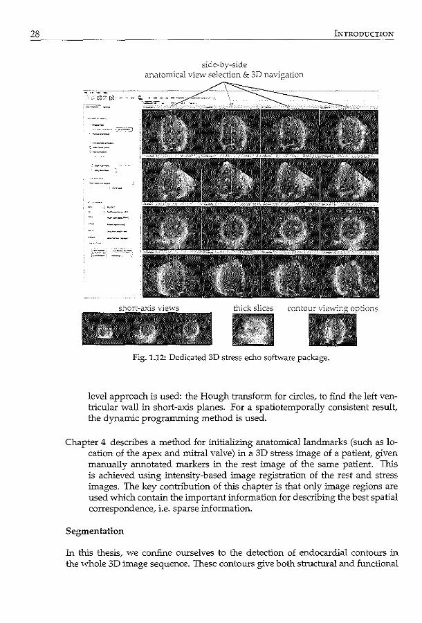
During the research of the automated methods, we have been developing a dedicated 3D stress echo software package, which is intended as a platform for automated analysis in clinical routine practice (see Fig. 1.12). On the one hand, this software should allow proper display of the stress echo images, to assist the traditional visual analysis and to improve the clinical workflow. In time, we wish to incorporate promising automated methods into the software, for obtaining and visualizing the measured clinical parameters.

27

Thesis outline 1.7.2

Initialization

As a starting point, initialization can be used to automatically select the appro­priate anatomical cross-sections for (visual or automated) stress analysis. This is important to allow accurate comparison of wall motion of each left ventricular segment between rest and stress. Also, it can be used as a starting point for au­tomated segmentation methods, to obtam a general location of the left ventricle and anatomical landmarks in the images.

Chapter 2 describes a method for automatically finding the anatomical markers in a 3D image using a statistical model of the left ventricular appearance. Agam, only sparse information is used to train the model. In order to match the model to a new image, a general optimization approach is used, which is very similar to the registration framework. By using a statistical model, the method corresponds to a more 'high-level' approach.

Chapter 3 describes an alternative method for automatically detecting the long­axis and mitral valve plane in a 3D image sequence. In this chapter, a 'low'

28 INTRODUCTION

side-by-side anatomical view selection & 3D navigation

G"tick slices

Fig. 1.12: Dedicated 3D stress echo softvvare package.

level approach is used: the Hough transform for circles, to find the left ven­tricular wall in short-axis planes. For a spatiotemporally consistent result, the dynamic programming method is used.

Chapter 4 describes a method for initializing anatomical landmarks (such as lo­cation of the apex and mitral valve) in a 3D stress image of a patient, given manually annotated markers in the rest image of the same patient. This is achieved using intensity-based image registration of the rest and stress images. The key contribution of this chapter is that only image regions are used which contain the important information for describing the best spatial correspondence, i.e. sparse :information.

Segmentation

In this thesis, we confine ourselves to the detection of endocardial contours in the whole 3D image sequence. These contours give both structural and functional

1.7 SCOPE AND OUTLINE

information on the left ventricle, which can be used to distinguish between normal and abnormal behavior.

Chapter 5 describes a method called the active appearance model for detecting the endocardial contours in a 3D image. Active appearance models, intro­duced in the past decade, have become a popular method for segmentation in medical images, because of their ability to model complex image infor­mation. In this chapter, a novel method for matching the model to a new image is evaluated, which is potentially capable of extending the range in which the model operates.

Chapter 6 describes a method for tracking an endocardial contour throughout an image sequence/ given the contour in one frame of the sequence. The method is partly based on a high-level statistical model of left ventricular motion, and on a low-level pixel-wise, frame-to-frame tracking of image regions. The latter is done using the differential optical flow method.

Chapter 7 describes a method for improving the tracking algorithm of Chapter 5 using low level temporal information of pixel intensity. As mentioned before, ultrasound images often contain many artifacts. The goal of the method is to derive information that can be used to indicate the probability of pixels as being a part of the left ventricular wall or as being obscured by typical ultrasound artifacts. The expectation-maximization method is used for this purpose.

Classification

In this thesis, we use supervised classification to discriminate between normal and abnormal motion. In particular, we focus on using features which are derived from the endocardial shapes.

Chapter 8 describes a novel feature representation which uses a statistical model of endocardial shape changes throughout the cardiac cycle. This represen­tation is obtained using a so-called orthomax rotation of the original shape model. The advantage is that this produces features that are more suitable for classifying wall motion of individual segments. The image sequences in this case are 2D, not 3D.

Clinical Application

The development of dedicated 3D stress echo software is, in our opinion, a vital step in promoting 3D stress echo in clinical practice. The software should, at its very basis, be able to display rest and stress images next to each other in a quadscreen-like format, with minimum observer input. This type of software has not been available commercially until very recently.

Chapter 9 describes the first clinical evaluation of the 3D stress echo software. By displaying rest and stress images, anatomically aligned, next to each other

29

30 INTRODUCTION

during visual wall motion scoring, we show that interobserver variabilities can be greatly reduced.

Discussion and conclusion

Chapter 10 discusses the investigated analysis methods and provides some gen­eral conclusions.

J\2". I '..; \ I :'; "-.__./ ~"

, \U . i.~

o\ ~ Appearance (;~~ (\ model based '.n ' \_____/•

registration for ''(C~\C';·~> ) t. . ~ ~ segmen 1ng sparse views -

In this chapter, appearance model segmentation and intensity-based image registra­tion were combined for detecting contours in 3D echocardiograms fully automatically. A sparse appearance model was built in 3D, consisting of the anatomical4-chamber, 2-chamber, and short-axis views, which were extracted from end-diastolic 3D data sets. The model was used to segment images in a registration framework, by opti­mizing appearance and pose parameters simultaneously. Encouraging results were obtained with leave-one-out experiments on 10 patient data sets. The method may help inter- and intrapatient comparison of images, and is intended as an initialization for a complete 3D segmentation.

0...-rivcd from: Sp=>c Appearance Model Based Registration and Scgmcnt.ltion of 3D Eclloardiogr.J.phk Inuges K.Y.E. Leung-, M. van Str..1lcn, G. v<m Burken, M.M. Voormolen, A. :--JemL'S, F.J. ten D.te, M.L. Gcleijn..-;c, N. de Jong.. A.F.W. v.m der Steen, J.H.C. Reiber, .md J.G. Bosch Proc IEEE Int Lltrason Symp 2006; 2413-6 =d Sp=.;:c Appe.:u.;mcc Model Based. Rcgist:t"ation of 3D Ult:t"J.Sound. Images K Y.E. L:>ung, M. Villl Str.Ucn.. G. v<m Burkcn.. MM. Voormolen, A. :-Jem<..'S, F.J. ten C:ltl', K. de Jong, A.F.W. v.m der Steen, J.H.C. Reiber, ;mdJ.G. Bosch Proc Mcd Imag Aug Reul2006; LNCS 4091; 236-43.

32 SPARSE APPEARA....'J"CE REGISTRATION

2.1 Introduction

Three dllnensional (3D) echocardiography is a non-invasive and relatively inex­pensive tool for visualizing the whole left ventricle (LV) over the complete cardiac cycle. New, fast 3D ultrasound imaging devices are entering the market and have potential in allowing a rapid, reliable, and user-friendly diagnosis of the left ventricle - provided that a suitable automated analysis method is available. A disadvantage of ultrasound, compared with other modalities, is the relatively complicated image appearance, which poses a considerable challenge for auto­matic segmentation and registration.

Many different approaches have been proposed for segmentation of the left ventricle in 3D echocardiography. For example, Angelini et a!. [2005] reported on a wavelet-based 4D echocardiographic image enhancement followed by a level­set LV segmentation. Gerard eta!. [2002] proposed a 2-simplex mesh deformable model to segment 3D echocardiographic images. Active appearance models (AAM) were used by Bosch et a!. [2002] to segment 2D+time echocardiographic images and were shown to be applicable in 3D ultrasound as well [Mitchell et a!., 2002]. AAMs seem especially suitable for the complicated ultrasound images, due to their ability to mimic the expert's segmentation decisions, especially in areas with typical ultrasound artifacts (such as echo drop-outs). However, AAMs as­sume that their parameters behave linearly, resulting in a limited lock-in range. Therefore, the technique requires adequate initialization of the model in a high di­mensional parameter space. Moreover, the models require cumbersome training before segmentation.

For alignment of different images of the left ventricle, image registration tech­niques can be employed. Registration of 3D ultrasound images has been explored by e.g. Rohling et a!. [1998] (3D gall bladder images) and Shekhar et a!. [2004] (3D stress echocardiography). However, nonrigid registration is computationally complex and optimization can be slow, if the images differ considerably.

In this chapter, we propose to exploit the advantages of both approaches by combining appearance modeling and intensity-based registration. To limit com­putational complexity, the model is built on a sparse subset of the 3D data, con­sisting of anatomical views of the 4-chamber, 2-chamber, and a short-axis image. Inspired by intensity based registration optimization, we match the appearance model to unseen images in a registration-like framework. This method will allow fully automatic extraction of the standard echocardiographic views. This will aid in the selection of images for inter- and intra-patient comparison and may provide an initialization for a complete 3D AAM.

2.2 METHODS 33

Methods 2.2

Sparse appearance modeling 2.2.1

The AAM [Cootes et al., 1998] is a well-known concept for segmentation of organs in medical imaging. This technique consists of modeling the variations in shape and texture within the target population, via statistical analysis of a training set of example segmentations. In short, principal component analysis (PCA) is applied to a training set of shapes (x = x + P,b,) and textures (g = g + P gbg) and to the combination of shape (b,) and texture (bg) parameter vectors,

b = ( ~:, ) = ( ~f[i~ ~~) ) , (2.1)

where x, g are the mean shape and texture and P ,, P g are the eigenvector matrices produced by the PCA. As such one model is obtained, with modes of variation P c

that describes the variations in appearance (shape and texture): b = P ,c [Cootes et al., 1998]. Using this model the training images can be approximated and new images are synthesized of whlch the appearance is known. Matching such a model to an unseen image aims at finding the best set of parameters c for whlch the synthesized image best matches to the unseen image.

Shape representation

We model the end-diastolic (ED) left ventricular (LV) endocardium in three or­thogonal planes, corresponding with the anatomical4- and 2-chamber views and one short-axis view at 1/3rd of the long axis. This model contains the standard anatomical views used in echocardiography and is similar to the sparse active shape model (configuration MV-4) of van Assen et al. [2006].

Training sets for the appearance model are created using the semi-automatic segmentation method by van Stralen et al. [2005b J. First, all full-cycle data sets are aligned to a common anatomical coordinate system, centered at the LV long-axis (LAX). The LAX is determined by manually annotating apex and mitral valve cen­ter iteratively, and selecting the correct 4-chamber image plane angle (see chapters 4 and 9). An example of the selected views is shown in Fig. 2.1. Full-cycle endo­cardial surfaces are obtained using pattern matching and dynamic programming [van Stralen et al., 2005b]. The contours for the training set are obtained by inter­secting the ED surface with the three image planes. An example of the manual segmentation is shown in Fig. 2.2.

Point correspondence is determined based on the LAX. For the long-axis con­tours, an atypical cylindrical/ spherical sampling is used. From the mitral valve to 3/4 of the apex-mitral valve height, the points are sampled cylindrically, whereas spherical sampling is applied in the remaining 1/4 region (Fig. 2.3). For the short-axis contours, radial sampling is applied with respect to the LAX point at 1/3 relative height. This results in 60 points for each long-axis view, 20 points for

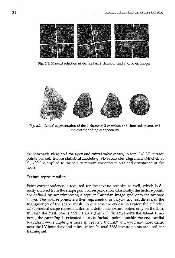
34 SPARSE APPEARANCE REGISTRATION

Fig. 2.1: Manual selection of 4-chamber, 2-charnber, and short-axis images.

Fig. 2.2: Manual segmentation of the 4-cham.ber, 2-chamber, and short-axis plane, and the corresponding 3D geometry.

the short-axis view, and the apex and mitral valve center; in totall42 3D surface points per set. Before statistical modeling, 3D Procrustes alignment [Mitchell et al., 2002] is applied to the sets to remove variation in size and orientation of the heart.

Texture representation

Point correspondence is required for the texture samples as well, which is di­rectly derived from the shape point correspondence. Classically, the texture points are defined by superimposing a regular Cartesian image grid onto the average shape. The texture points are then represented in barycentric coordinates of the triangulation of the shape mesh. In our case we choose to exploit the cylindri­cal/ spherical shape representation and define the texture points only on the lines through the mesh points and the LAX (Fig. 2.3). To emphasize the salient struc­tures, the sampling is extended so as to include points outside the endocardial boundary, and sampling is more sparse near the LAX and apex, and more dense near the LV boundary and mitral valve. In total 8668 texture points are used per training set.

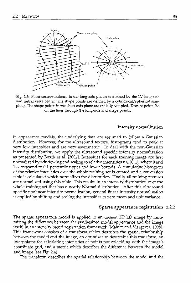
2.2 METHODS

Apex.

Fig. 2.3: Point correspondence in the long-axis planes is defined by the LV long-axis and mitral valve center. The shape points are defined by a cylindrical/ spherical sam­pling. The shape points in the short-axis plane are radially sampled. Texture points lie

on the lines through the long-axis and shape points.

Intensity normalization

In appearance models, the underlying data are assumed to follow a Gaussian distribution. However, for the ultrasound texture, histograms tend to peak at very low intensities and are very asymmetric. To deal with the non-Gaussian intensity distribution, we apply the ultrasound specific intensity normalization as presented by Bosch et al. [2002]. Intensities for each training image are first normalized by windowing and scaling to relative intensities r E [0, 1], where 0 and 1 correspond to 0.1-percentile upper and lower bounds. A cumulative histogram of the relative intensities over the whole training set is created and a conversion table is calculated which normalizes the distribution. Finally, all training textures are normalized using this table. This results in an intensity distribution over the whole training set that has a nearly Normal distribution. After this ultrasound specific nonlinear intensity normalization, general linear intensity normalization is applied by shifting and scaling the intensities to zero mean and unit variance.

35

Sparse appearance registration 2.2.2

The sparse appearance model is applied to an unseen 3D ED image by mini­mizing the difference between the synthesized model appearance and the image itself, in an intensity based registration framework [Maintz and Viergever, 1998]. This framework consists of a transform which describes the spatial relationship between the model and the image, an optimizer to determine this transform, an interpolator for calculating intensities at points not coinciding with the image's coordinate grid, and a metric which describes the difference between the model and image (see Fig. 2.4).

The transform descnbes the spatial relationship between the model and the

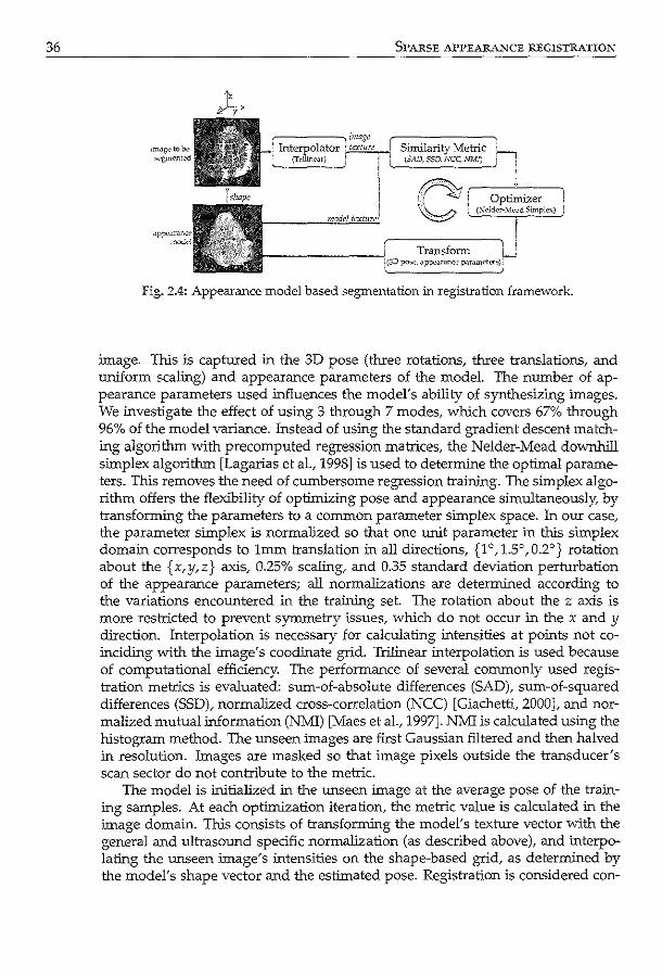
36 SPARSE APPE.AR.A.i.~CE REGISTRATION

Fig. 2.4: Appearance model based segmentation in registration framework.

image. This is captured in the 3D pose (three rotations, three translations, and uniform scaling) and appearance parameters of the model. The number of ap­pearance parameters used influences the model's ability of synthesizing images. We investigate the effect of using 3 through 7 modes, whlch covers 67% through 96% of the model variance. Instead of using the standard gradient descent match­ing algorithm with precomputed regression matrices, the Nelder-Mead downhill simplex algorithm [Lagarias et al., 1998] is used to determine the optimal parame­ters. This removes the need of cumbersome regression training. The simplex algo­rithm offers the flexibility of optimizing pose and appearance simultaneously, by transforming the parameters to a common parameter simplex space. In our case, the parameter simplex is normalized so that one unit parameter in this simplex domain corresponds to 1mm translation in all directions, {1 o, 1.5°, 0.2°} rotation about the {x,y,z} axis, 0.25% scaling, and 0.35 standard deviation perturbation of the appearance parameters; all normalizations are determined according to the variations encountered in the tra:i.rting set. The rotation about the z axis is more restricted to prevent synunetry issues, whlch do not occur in the x and y direction. Interpolation is necessary for calculating intensities at points not co­inciding with the image's coodinate grid. Trilinear interpolation is used because of computa tiona! efficiency. The performance of several commonly used regis­tration metrics is evaluated: sum-of-absolute differences {SAD), sum-of-squared differences (SSD), normalized cross-correlation (NCC) [Giachetti, 2000], and nor­malized mutual information {NMl) [Maes et al., 1997]. NM1 is calculated using the hlstogram method. The unseen images are first Gaussian filtered and then halved in resolution. Images are masked so that image pixels outside the transducer's scan sector do not contribute to the metric.

The model is initialized in the unseen image at the average pose of the train­ing samples. At each optimization iteration, the metric value is calculated in the image domain. This consists of transforming the model's texture vector with the general and ultrasound specific normalization (as described above), and interpo­lating the unseen image's intensities on the shape-based grid, as determined by the model's shape vector and the estimated pose. Registration is considered con-

2.3 REsuLTS

verged if the metric value differences between the simplex vertices are less than 10-4 for SAD and SSD and 10-6 for NCC and NMI, and if the Euclidean distance between the vertices are less than 10-3 After convergence, the optimization is restarted at the found minimum to check for suboptimality. Mean registration times of the algorithm, implemented in MATLAB® (version 6.5.0, release 13, The Math Works, Inc.), not optimized for speed, on a 2.8GHz Intel® Pentium® 4 pro­cessor are 4.6min, 5.7min, 5.1min, 1.8min for the SAD, SSD, NCC, NMI metrics, respectively.

37

Data description 2.2.3

Full-cycle 3D data sets of the LV were acquired from 10 patients, obtained in the apical position using the Philips Sonos 7500 ultrasound machine. The sets contained 160 x 144 x 208 voxels at a resolution of 1.1 x 1.1 x 0.7mm3 (length x width x depth). Appearance models were built and matched on 3D end-diastolic (ED) volumes. ED was defined as the time point of the ECG R-peak.

Results 2.3

The sparse appearance registration algorithm is tested in a leave-one-out fashion, on ED data sets from 10 patients. An example of the registration results (NCC metric, 7 modes), together with the manual segmentation and the initial position of the model, is given in Fig. 2.5. The segmentation results are in good agreement with the manual segmentation.

Fig. 2.6 shows the effect of increasing the number of modes in the appearance model, for the investigated metrics. Mean point-to-point and point-to-surface er­rors with respect to the manual segmentation are given. The full 3D manually seg­mented surface is used to calculate the point-to-surface errors. An improvement in both error measures can be perceived for all metrics and number of modes investigated. Best results are obtained with the NCC metric using the largest number of modes in the model. The NCC metric performs better than SAD or SSD, which may be because the use of SAD and SSD implicitly assumes that the model and image only differ by Gaussian noise, whereas a less strict assumption of a linear relationship between the intensity values is made for NCC. Using NMI on the other hand, no direct assumption is made in the relation between model and image intensities. Therefore, pixels representing blood and tissue may be inversely matched with NMI. This may potentially drive the shape component of the appearance model in the wrong direction, since matching is based on the intensities only. Also, there may be some partial volume effects since linear inter­polation is used, instead of partial volume interpolation. Further investigation is needed to improve NMI in this registration framework. An advantage of using NMI may be the ability to exchange models between different modalities.

In this chapter, we chose a sparse appearance model consisting of three most common anatomical views. However, further investigation of the sparseness of

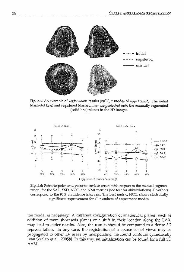
38 SPARSE APPEARANCE REGISTRATION

initial

registered

---manual

Fig. 2.5: An example of registration results (NCC, 7 modes of appearance). The initial (dash-dot line) and registered (dashed line) are projected onto the manually segmented

(solid line) planes in the ZD images.

16

14

3

Point to Point

78% 5

SS% 7

96%

5.5

2.5

2

1.5 3

67%

Point to Surface

3 78%

6 91%

:; <!ppearance modes I cover.:~ge

-·-·-initial

-+SAD -"9 ·SSD

-3-NCC ---·:--1\:MI

7 96%

fig. 2.6: Point-to-point and point-to-surface errors with respect to the manual segmen­tation, for the SAD, SSD, NCC, and NMI metrics (see text for abbreviations). Errorbars correspond to the 95% confidence .intervals. The best metric, NCC, shows statistically

significant improvement for all numbers of appearance modes.

the model is necessary. A different configuration of anatomical planes, such as addition of more short-axis planes or a shift in their location along the LAX, may lead to better results. Also, the results should be compared to a dense 3D representation. In any case, the registration of a sparse set of views may be propagated to other LV areas by interpolating the found contours cylindrically [van Stralen et al., 2005b]. In this way, an initialization can be found for a full 3D AAM.

2.4 CoNCLUSIONS

Conclusions 2.4

We have developed a sparse appearance model based registration algorithm for fully automatic extraction of standard anatomical views in 3D echocardiographic images. A sparse appearance model is built on manually segmented 4-chamber, 2-chamber, and short-axis planes of 3D end-diastolic data sets. Adaptations are made to accommodate for the non-Gaussian distribution of ultrasound intensities. Furthermore, image intensities are modeled and matched in a shape-dependent grid, which circumvents cumbersome image warping. In the matching phase, the model is used to segment unseen images in an intensity-based registration framework. Evaluation on 10 patients data sets revealed improvement in the LV segmentation. The registration method can be used to find the global anatomi­cal coordinate system in ultrasound images and may serve as the basis of a full 3D I 4D segmentation algorithm.

39

Detection of the left ventri-cular long axis and the mitral valve plane Automated segmentation approaches for the left ventricle (LV) in 3D echocardiogra­phy often rely on manual initialization. So far/ little effort has been put in automating the initialization procedure to get to a fully automatic segmentation approach. We propose a fully automatic method for the detection of the LV long axis (LAX) and the mitral valve plane (MVP) over the full cardiac cycle. Our method exploits the cyclic motion of the LV and therefore detects salient structures in a time-continuous way. Probabilities to candidate LV center points are assigned through a Hough trans­form for circles. The LAX is detected by combining dynamic programming detec­tions on these probabilities in 3D and 2D+time to obtain a time continuous solution. Subsequently, the mitral valve plane is detected using the previously detected LAX. Automatic detection was evaluated using patient data acquired with the fast rotating ultrasound (FRU) transducer and with the Philips Sonos 7500 ultrasound system with the X4 matrix transducer. For the FRU data, the LAX was estimated with a distance error of 2.85±1.70mm and an angle of 5.25±3.17'; the MVP was estimated with a dis­tance of -1.54 ± 4.3lmm. For the matrix data, these distances were 1.96±1.30mm with an angle error of 5.95±2.11 ° and -1.66±5.27mm for the mitral valve plane. These re­sults confirm reliable detection of the LAX and MVP, allowing automatic initialization of 3D segmentation approaches.

©World Federation for Ultra...;ound in Medicine & Biolq,-y. Reprinted, with pcrmL~ion, fr-om: Time contim.1ous detection of the left ventricular long axis and the mitral v:Uve plane in three-dimensional cchocardiography. M. van Stralcn, K Y.E. Leung. M.:vL Voormolcn, K. de Jons,. A.F.W. vJ.n dcr Steen, J.H.C. Reiber, and J.G. Bosch Ultra:<ound Mcd Biol2008; 34(2); 196-207.

42 LONG AXlS AND :M:ITRAL VALVE DETECTION

3.1 Introduction and literature

3D echocardiography is an increasingly widely available acquisition technique for assessment of left ventricular (LV) function, which is non-invasive, relatively cheap and portable. Due to the rapid increase of the use of this modality for diag­nosing global and regional LV function, valvular disease, etc. there is a growing demand for objective, reproducible and automated techniques for identification of salient structures and quantification of left ventricular function.

Recently, several approaches for automated endocardial contour detection have been proposed, reporting success in measuring global functional parame­ters [Angelini et a!., 2001; Corsi et al., 2002; Gerard et al., 2002; Kiihl eta!., 2004; van Stralen et al., 2005b; Zagrodsky et al., 2005], and significantly decreasing the amount of user interaction that is needed for these measurements. Also, several quantification tools have already become available on commercial 3D echocardio­graphy (3DE) systems. Although time can be gained by using these tools, reliable quantification of important clinical parameters is still very labor intensive and not yet ready for use in daily clinical routine. This requires techniques that need min­imal or no user interaction. Moreover, automating the initialization procedure of such methods would also eliminate inter- and intraobserver variability from the analysis, increasing the reproducibility of the analysis.

Most previously presented methods for the quantification of LV function re­quire some manual initialization. Initialization is done either by explicitly arno­tating the apex, a number of points on the endocardial border or the mitral valve [Corsi et al., 2002; van Stralen eta!., 2005b], or by indicating the LV position and dimensions by arnotations [Angelini et al., 2001; Gerard et a!., 2002; Ki.ihl et al., 2004].

Although much attention has been paid to minimize this user interaction for automated contour detection, little effort has been put in developing dedicated au­tomatic initialization procedures, which focus on automatically detecting salient structures in 3D echocardiography (3DE). Stetten and Pizer [1999] attempt to de­tect the apex and mitral valve center using medial-node models. Veronesi et al. [2006] describe a method for automated detection of the LV LAX based on op­tical flow, but it still needs manual initialization. The segmentation method by Zagrodsky et a!. [2005] is initialized using a time-consuming registration with a pre-segmented template image.

Automated initialization has received more attention for segmentation of car­diac magnetic resonance (MR) images. We were inspired by work of MUller et a!. [2005]; van der Geest et al. [1997], who detect the LV center in short-axis MR images using a Hough transform [Ballard, 1981] for circles, for initialization of automated endocardial border detection.

We propose a fully automatic method for reliable estimation of the position of the mitral valve and the orientation of the left ventricular long axis for apical 3D echocardiographic images of clinical quality. The computation costs are relatively low and the method is easily adaptable, which makes it a valuable starting point for various high-level segmentation techniques.

3.2 MATERIALS AND METHODS

Materials and methods 3.2

We propose a method for finding the long axis (LAX) of the left ventricle and the mitral valve plane (MVP). Such a method should be capable of dealing with typical ultrasound acquisition characteristics, such as inhomogeneous image in­tensities, speckle and partial dropout of the myocardium.

The detection of these salient structures of the LV is achieved by a few robust consecutive steps (Fig. 3.1). At first, the LAX is detected by locating the main circular structure in a number of planes perpendicular to the (apical) acquisition axis over time, using a Hough transform for circles (Fig. 3.1a-b ). Consecutively, multidimensional dynamic programming is applied in 3D and 2D+time to locate probable LV centers (Fig. 3.1c-e). Fitting a line through the LV centers in each cardiac phase results in the final LAX (Fig. 3.1£). The estimate for the LAX is used for finding the MVP, in a spherical projection of the LV (Fig. 3.1g).

43

Detection of long axis 3.2.1

For the detection of the LAX in the apical3DE image sequences of the left ventricle we choose to detect the LV centers in planes perpendicular to the acquisition axis. These planes resemble regular 2D short-axis acquisitions of the LV (Fig. 3.2a). They are extracted by dividing the image data into a number of slices L and integrating the data within each slice along the acquisition axis. We exclude the upper 10% and the lower 10% of the image volume from analysis to remove influence of near-field noise and to exclude the lower part of the image that has been left empty, respectively.

We aim at detecting the center of the endocardial border, which appears in these planes as the inner edge of the main circular structure, using a Hough transform [Ballard, 1981] for circles (HT,). The Hough transform is known to be robust to partial dropout of target structures and invariant to the circle radius.

For location of possible circle centers, the HT, utilizes the image gradient G as a measure for edge orientation and the gradient magnitude II Gil as a measure for edge strength. G is implemented as a convolution with a Gaussian derivative at a scale cr.

We apply a thresholding operation on the gradient image G to remove influ­ence from noise in the background and use only the strong gradients. We define the threshold as the gradient value which corresponds with a certain percentile value Zt of the histogram of all gradient images, in order to be invariant to global contrast changes throughout the different acquisitions. The optimal value of g, is determined experimentally. The HT, transforms the gradient image into a prob­ability map for circle centers, the accumulator image A (Fig. 3.2b ), with the same dimensions as G, using the gradient magnitude I! Gil as a weighing function for

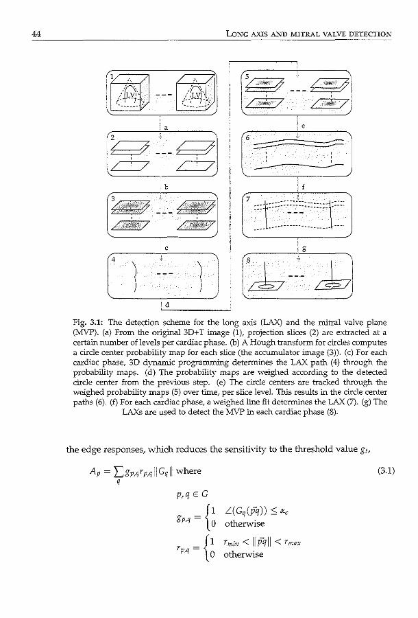
44 LONG AXIS AND MITRAL VALVE DETECTION

;a

~ ~ :7 ~ /

;b

' ' /.,;w. / /./ii!il'/

c

~ /

iiil"!!W''

' ' dill!¢'/

' '

/j /

( ,.f!!fiif:Y

/ ,./ ·,

' '

/j

/

------­i f

Fig. 3.1: The detection scheme for the long axis (LAX) and the mitral valve plane (MVP). (a) From the original 3D+ T image (n projection slices (2) are extracted at a certain number of levels per cardiac phase. (b) A Hough transform for circles computes a circle center probability map for eacb slice (the accumulator image (3)). (c) For eacb cardiac phase, 3D dynamic programming determines the LAX path (4) through the probability maps. (d) The probability maps are weighed according to the detected circle center from the previous step. (e) The circle centers are tracked through the weighed probability maps (5) over time, per slice level. This results in the circle center paths (6). (f) For eacb cardiac phase, a weighed line fit determines the LAX (7). (g) The

LAXs are used to detect the MVP in eacb cardiac phase (8).

the edge responses, whlch reduces the sensitivity to the threshold value g,,

Ap = Lgp,qrp,q]IGqll where q

p,q E G

gp,q = g rp,q = {~

L( Gq (pq)) :S o:.e otherwise

rmin < IIP'/11 < rmax

otherwise

(3.1)

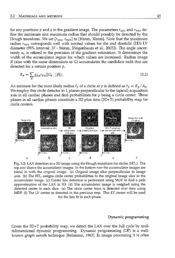
3.2 MATERIALS AND METHODS

for any positions p and q in the gradient image. The parameters r min and r max de­fine the minimum and maximum radius that should possibly be detected by the Hough transform. We set [rmin• Ymaxl to [lOmm, 30mm]. Note that the maximum radius rmax corresponds well with normal values for the end diastolic (ED) LV diameter (95% interval: 37 - 56mm, [Feigenbaum et al., 2005]). The angle uncer­tainty IX.c is related to the precision of the gradient estimation. It determines the width of the accumulator region for which values are increased. Radius image R (also with the same dimensions as G) accumulates the candidate radii that are detected for a certain position p,

Rp = Lgp,qYp,qiiGqiiiiJ?illl· (3.2) q

An estimate for the most likely radius fp of a circle at pis defined as fp = Rp/ Ap· We employ this circle detector in L planes perpendicular to the (apical) acquisition axis in all cardiac phases and find probabilities for p being a circle center. These planes in all cardiac phases constitute a 3D plus time (3D+ T) probability map for circle centers.

Acrumuhltor >lice 30 We<f!;hted ---+ ---+ uccumulutor ---+ "ccumulutor ,.[kc -o.o"='''""

with

a b c d e

Fig. 3.2: LAX detection in a 3D image us:ing the Hough transform for circles (HTc). The top row shows the accumulator images. In the bottom row the accumulator images are blend in vvith the original image. (a) Original image slice perpendicular to image axis. (b) The HTc assigns circle center probabilities to the original image slice in the accumulator image. (c) Center line detection is performed using MDP to find a path approximation of the LAX in 3D. (d) The accumulator image is weighed using the detected center in each slice. (e) The circle center trace is detected over time using MDP. (f) The LV center as detected in the previous step. This LV center will be used

for the line fit in each phase.

Dynamic programming

Given the 3D+ T probability map, we detect the LAX over the full cycle by mul­tidimensional dynamic programming. Dynamic programming (DP) is a well­known graph search technique [Bellmann, 1965]. In image processing it is often

45

46 LONG AXIS AND MITRAL VALVE DETECTION

2 1

'6 '5 i

5 1

' 1--=2-~3=---, --:4-+2::--' I L • i

~------· : 1 i 2 ? I 3 . I : , - ~ ~ I ~·-,--f-ec-­i 3 i 1 ' 3

!

a

4

i(]

Wil

!2 ~4 :2

L___~,2' 6 5! 6 -vIs 5

II, t::l,l 7

-zf~> 414

1'1 ,' 2 i 2

/' 5 1. 3i •

3 1 i 3 I~

3 : 2

b

1 1 2

3

•

4

i"'O ... M-1

:2 ! 4 i 2 ! 1 I --~-----1-----1.---- I ! 2 i 61 8 9: i 6 I 5 ! 5 ' 1

i , ! ; I ,

6!/7!/g!/s: z 2 /,3;--'!,4 ./·2_! c ' 2 !,/ 4 !,/ 7 6 " T--~_? _ _,--_--2~,-~_--~-"!

' 3: 7! '3 ~-~z_s, si

c optim;;~l p.:ath

Fig. 3.3: Dynamic programming. (a) Initial cost matrix. The costs cij for each node nif

are shown in the top-left of each node. (b) Computation of the cumulative cost matrix. Cumulative costs w1j are shown in bold for the nodes ill the first tvvo columns. The dashed arrows represent the edges eijk between the nodes. The bold edge is the edge for which the cumulative costs for the bold node are minimal. (c) The complete cumu­lative cost matrix with, for each node, a reference (represented by k) to the previous column. The optimal path is backtracked from the node with lowest cumulative costs

in the last column/ following the references (solid arrows).

referred to as a minimum cost algorithm for finding a connective path through a 2D cost image [Amini et al, 1990; Sonka et aL, 1999]. In this classical approach (Fig. 3.3), the pixels in the cost image v (of M rows and N columns) act as nodes nij(i = 0, ... , M- 1; j = 0, ... , N- 1) in a directed graph, the corresponding pixel values Vfj as the node costs c1j (i.e. the circle center probabilities). The directional edges in the graph are defined by imposing a connectivity constraint, the maxi­mum step size 5. This step size limits the number of neighbors (25 + 1) to which a node nij in column j is connected in the next column j + L We denote the di­rected edge eijk' the edge from nij to ni+k.j+l' where k E [-5,5]. Additional costs aijk may be assigned to edge eijk·

Dynamic programming is a technique that greedily searches to find the cheap­est path from column 0 to N- 1. This path is found by computing the cumulative cost wij for each node nijf

w··= min (w·~k-~1+"'--k+c--)where !J k=-s ... s 1 ,J 1J 1J

(3.3)

The value of k for which Wfj is minimal is stored with each corresponding node. The optimal path is then easily found by backtracking from the node ni,N~l' for which

wi,N~! =. min (wi,N~!) l=O ... M~l

(3.4)

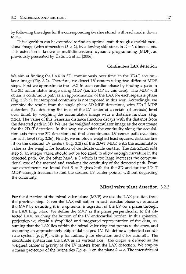
3.2 MATERIALS AND METHODS

by following the edges for the corresponding k-value stored with each node, down to ni,O·

This algorithm can be extended to find an optimal path through a multidimen­sional image (with dimension D > 2), by allowing side steps in D - 1 dimensions. This extension is known as multidimensional dynamic programming (MDP), as previously presented by Dzumcu eta!. [2006].

Continuous LAX detection

We aim at finding the LAX in 3D, continuously over time, in the 3D+ T accumu­lator image (Fig. 3.2). Therefore, we detect LV centers using two different MDP steps. First we approximate the LAX in each cardiac phase by finding a path in the 3D accumulator image using MDP (i.e. 2D DP in this case). The MDP will obtain a continuous path as an approximation of the LAX for each separate phase (Fig. 3.2b,c), but temporal continuity is not imposed in this way. Accordingly, we combine the results from the single-phase 3D MDP detections, with 2D+ T MDP detections (i.e. detecting the trace of the LV center at a certain (short-axis) level over time), by weighing the accumulator image with a distance function (Fig. 3.2d). The value of this Gaussian distance function decays with the distance from the detected path in 3D. We use the weighed accumulator image as the cost image for the 2D+ T detection. In this way, we exploit the continuity along the acquisi­tion axis from the 3D detection and find a continuous LV center path over time for each level (Fig. 3.2e). Finally, we employ a weighed least squared distance line fit on the detected LV centers (Fig. 3.2£) of the 2D+ T MDP, with the accumulator value as the weight, for location of candidate circle centers. The maximum side step S, an integer value, should not be too small to allow enough curvature in the detected path. On the other hand, a S which is too large increases the computa­tional cost of the method and weakens the continuity of the detected path. From our experiments we found that S = 2 gives both for the 3D and for the 2D+ T MDP enough freedom to find the desired LV center points, without degrading the continuity.

47

Mitral valve plane detection 3.2.2

For the detection of the mitral valve plane (MVP) we use the LAX position from the previous step. Given the LAX estimation in each cardiac phase we estimate the MVP by detecting it in a spherical integration of the LV on a plane through the LAX (Fig. 3.4a). We define the MVP as the plane perpendicular to the de­tected LAX, touching the bottom of the LV endocardial border. In this spherical projection we obtain a simplified and integrated representation of the data, as­suming that the LAX lies within the mitral valve ring and points to the apex, and assuming an approximately ellipsoidal shaped LV. We define a spherical coordi­nate system (p, rp, 8), with p for radius, rp for elevation and e for azimuth. The coordinate system has the LAX as its vertical axis. The origin is defined as the weighed center of gravity of the LV centers from the LAX detection. We employ a mean projection of the intensities I(p, rp,.) on the plane e = c. The intensities of

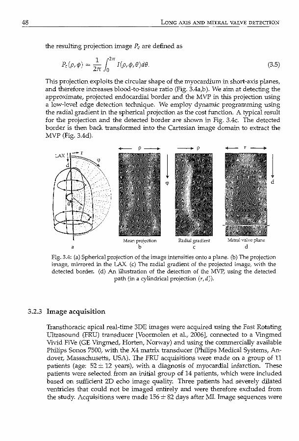
48 LONG AXIS AND MITRAL VALVE DETECTION

the resulting projection image P, are defined as

1 [2" P,(p,<fJ) = Zrr Jo I(p,</J,&)de. (3.5)

This projection exploits the circular shape of the myocardium in short-axis planes, and therefore increases blood-to-tissue ratio (Fig. 3.4a,b ). We aim at detecting the approximate, projected endocardial border and the MVP in this projection using a low-level edge detection technique. We employ dynamic programming using the radial gradient in the spherical projection as the cost function. A typical result for the projection and the detected border are shown in Fig. 3.4c. The detected border is then back transformed into the Cartesian image domain to extract the MVP (Fig. 3.4d).

a

+-- p--+

Me<111 projection b

--+ p

Radial gradient

c

+--f----+

11itral valve plane

d

1 d

Fig. 3.4: (a) Spherical projection of the image intensities onto a plane. (b) The projection image, mirrored in the LAX. (c) The radial gradient of the projected image, with the detected border. (d) An illustration of the detection of the MVP, using the detected

path (in a cylindrical projection (r,d)).

3.2.3 Image acquisition

Transthoracic apical real-time 3DE images were acquired using the Fast Rotating Ultrasound (FRU) transducer [Voormolen et a!., 2006], connected to a Vingmed Vivid FiVe (GE Vmgmed, Harten, Norway) and using the commercially available Philips Sonos 7500, with the X4 matrix transducer (Philips Medical Systems, An­dover, Massachusetts, USA). The FRU acquisitions were made on a group of 11 patients (age: 52± 12 years), with a diagnosis of myocardial infarction. These patients were selected from an initial group of 14 patients, which were included based on sufficient 2D echo image quality. Three patients had severely dilated ventricles that could not be imaged entirely and were therefore excluded from the study. Acquisitions were made 156 ± 82 days after MI. Image sequences were

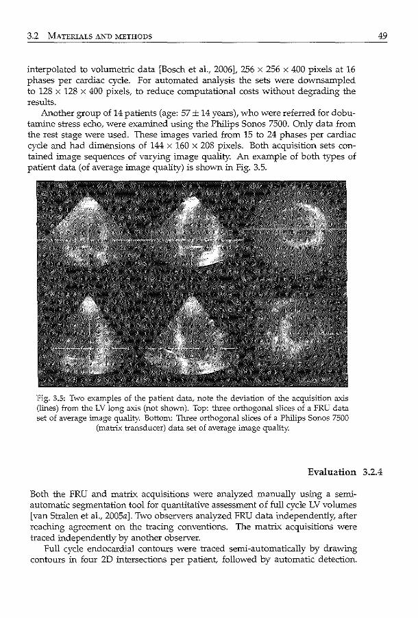
3.2 MATERIALS AND METHODS

interpolated to volumetric data [Bosch et al., 2006], 256 x 256 x 400 pixels at 16 phases per cardiac cycle. For automated analysis the sets were downsampled to 128 x 128 x 400 pixels, to reduce computational costs without degrading the results.

Another group of 14 patients (age: 57± 14 years), who were referred for dobu­tamine stress echo, were examined using the Philips Sonos 7500. Only data from the rest stage were used. These images varied from 15 to 24 phases per cardiac cycle and had dimensions of 144 x 160 x 208 pixels. Both acquisition sets con­tained image sequences of varying image quality. An example of both types of patient data (of average image quality) is shown in Fig. 3.5.

fig. 3.5: Two examples of the patient data, note the deviation of the acquisition axis (lines) from the LV long axis (not shown). Top: three orthogonal slices of a FRU data set of average image quality. Bottom: 1hree orthogonal slices of a Philips Sonos 7500

(matrix transducer) data set of average image quality.

49

Evaluation 3.2.4

Both the FRU and matrix acquisitions were analyzed manually using a semi­automatic segmentation tool for quantitative assessment of full cycle LV volumes [van Stralen et al., 2005a]. Two observers analyzed FRU data independently, after reaching agreement on the tracing conventions. The matrix acquisitions were traced independently by another observer.

Full cycle endocardial contours were traced semi-automatically by drawing contours in four 2D intersections per patient, followed by automatic detection.

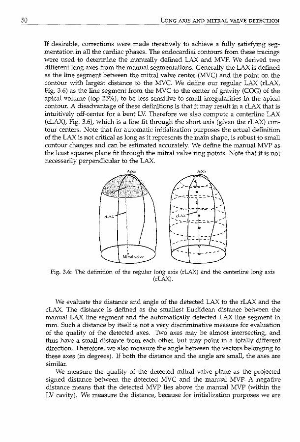
50 LONG AXIS AND MITRAL VALVE DETECTION

If desirable, corrections were made iteratively to achieve a fully satisfying seg­mentation in all the cardiac phases. The endocardial contours from these tracings were used to determine the manually defined LAX and MVP. We derived two different long axes from the manual segmentations. Generally the LAX is defined as the line segment between the mitral valve center (MVC) and the point on the contour with largest distance to the MVC. We define our regular LAX (rLAX, Fig. 3.6) as the line segment from the MVC to the center of gravity (COG) of the apical volume (top 25%), to be less sensitive to small irregularities in the apical contour. A disadvantage of these definitions is that it may result in a rLAX that is intuitively off-center for a bent LV. Therefore we also compute a centerline LAX (cLAX), Fig. 3.6), which is a line fit through the short-axis (given the rLAX) con­tour centers. Note that for automatic initialization purposes the actual definition of the LAX is not critical as long as it represents the main shape, is robust to small contour changes and can be estimated accurately. We define the manual MVP as the least squares plane fit through the mitral valve ring points. Note that it is not necessarily perpendicular to the LAX.

' . Mitral v;;tlw

Fig. 3.6: The definition of the regular long a"Xis (rLAX) and the centerline long axis (cLAX).

We evaluate the distance and angle of the detected LAX to the rLAX and the cLAX. The distance is defined as the smallest Euclidean distance between the manual LAX line segment and the automatically detected LAX line segment in mm. Such a distance by itself is not a very discriminative measure for evaluation of the quality of the detected axes. Two axes may be almost intersecting, and thus have a small distance from each other, but may point in a totally different direction. Therefore, we also measure the angle between the vectors belonging to these axes (in degrees). If both the distance and the angle are small, the axes are similar.

We measure the quality of the detected mitral valve plane as the projected signed distance between the detected MVC and the manual MVP. A negative distance means that the detected MVP lies above the manual MVP (within the LV cavity). We measure the distance, because for initialization purposes we are

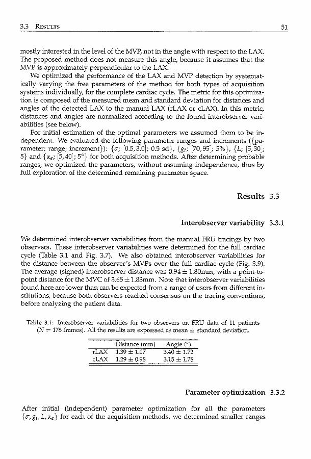
3.3 RESULTS

mostly interested in the level of the MVP, not in the angle with respect to the LAX. The proposed method does not measure this angle, because it assumes that the MVP is approximately perpendicular to the LAX.

We optimized the performance of the LAX and MVP detection by systemat­ically varying the free parameters of the method for both types of acquisition systems individually, for the complete cardiac cycle. The metric for this optimiza­tion is composed of the measured mean and standard deviation for distances and angles of the detected LAX to the manual LAX (rLAX or cLAX). In this metric, distances and angles are normalized according to the found interobserver vari­abilities (see below).

For initial estimation of the optimal parameters we assumed them to be in­dependent. We evaluated the following parameter ranges and increments ( {pa­rameter; range; increment}): {a-; [0.5,3.0]; 0.5 sd}, {g1; [70,95]; 5%}, {L; [5,30]; 5} and {«e; [5,40]; 5°} for both acquisition methods. After determining probable ranges, we optimized the parameters, without assuming independence, thus by full exploration of the determined remaining parameter space.

Results

51

Interobserver variability 3.3.1

We determined interobserver variabilities from the manual FRU tracings by two observers. These interobserver variabilities were determined for the full cardiac cycle (Table 3.1 and Fig. 3.7). We also obtained interobserver variabilities for the distance between the observer's MVPs over the full cardiac cycle (Fig. 3.9). The average (signed) interobserver distance was 0.94 ± l.SOmm, with a point-to­point distance for the MVC of 3.65 ± 1.83mm. Note that interobserver variabilities found here are lower than can be expected from a range of users from different in­stitutions, because both observers reached consensus on the tracing conventions, before analyzing the patient data.

Table 3.1: Interobserver variabilities for two observers on FRU data of 11 patients (N = 176 frames). All the results are expressed as mean± standard deviation.

Distance (mm) rLAX 1.39 ± 1.07 cLAX 1.29 ± 0.98

Angten 3.40 ± 1.72 3.15 ± 1.78

Parameter optimization 3.3.2

After initial (independent) parameter optimization for all the parameters { o-, g1, L, «e} for each of the acquisition methods, we determined smaller ranges

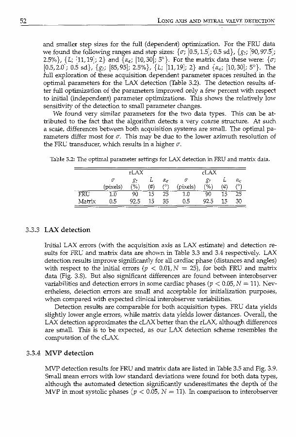
52 LONG AXIS A._"'JD MITRAL VALVE DETECTION

and smaller step sizes for the full (dependent) optimization. For the FRU data we found the following ranges and step sizes: { CT; [0.5, 1.5]; 0.5 sd }, {g,; [90, 97.5]; 2.5%}, {L; [11, 19]; 2} and {a,; [10,30]; 5°}. For the matrix data these were: {CT; [0.5,2.0]; 0.5 sd}, {g1; [85,95]; 2.5%}, {L; [11,19]; 2} and {ae; [10,30]; 5°}. The full exploration of these acquisition dependent parameter spaces resulted in the optimal parameters for the LAX detection (Table 3.2). The detection results af­ter full optimization of the parameters improved only a few percent with respect to initial (independent) parameter optimizations. This shows the relatively low sensitivity of the detection to small parameter changes.

We found very similar parameters for the two data types. This can be at­tributed to the fact that the algorithm detects a very coarse structure. At such a scale, differences between both acquisition systems are small. The optimal pa­rameters differ most for CT. This may be due to the lower azimuth resolution of the FRU transducer, which results in a higher CT.

Table 3.2: The optimal parameter settings for LAX detection in FRU and matrix data.

rLAX cLAX IT g, L a, IT g, L a,

(pixels) (%) (#) n (pixels) (%) (#) COl FRU 1.0 90 15 25 1.0 90 15 25 Matrix 0.5 92.5 15 35 0.5 92.5 15 30

3.3.3 LAX detection

Initial LAX errors (with the acquisition axis as LAX estimate) and detection re­sults for FRU and matrix data are shown in Table 3.3 and 3.4 respectively. LAX detection results improve significantly for all cardiac phase (distances and angles) with respect to the initial errors (p < 0.01, N = 25), for both FRU and matrix data (Fig. 3.8). But also significant differences are found between interobserver variabilities and detection errors in some cardiac phases (p < 0.05, N = 11). Nev­ertheless, detection errors are small and acceptable for initialization purposes, when compared with expected clinical interobserver variabilities.

Detection results are comparable for both acquisition types. FRU data yields slightly lower angle errors, while matrix data yields lower distances. Overall, the LAX detection approximates the cLAX better than the rLAX, although differences are small. This is to be expected, as our LAX detection scheme resembles the computation of the cLAX.

3.3.4 MVP detection

MVP detection results for FRU and matrix data are listed in Table 3.5 and Fig. 3.9. Small mean errors with low standard deviations were found for both data types, although the automated detection significantly underestimates the depth of the MVP in most systolic phases (p < 0.05, N = 11). In comparison to interobserver

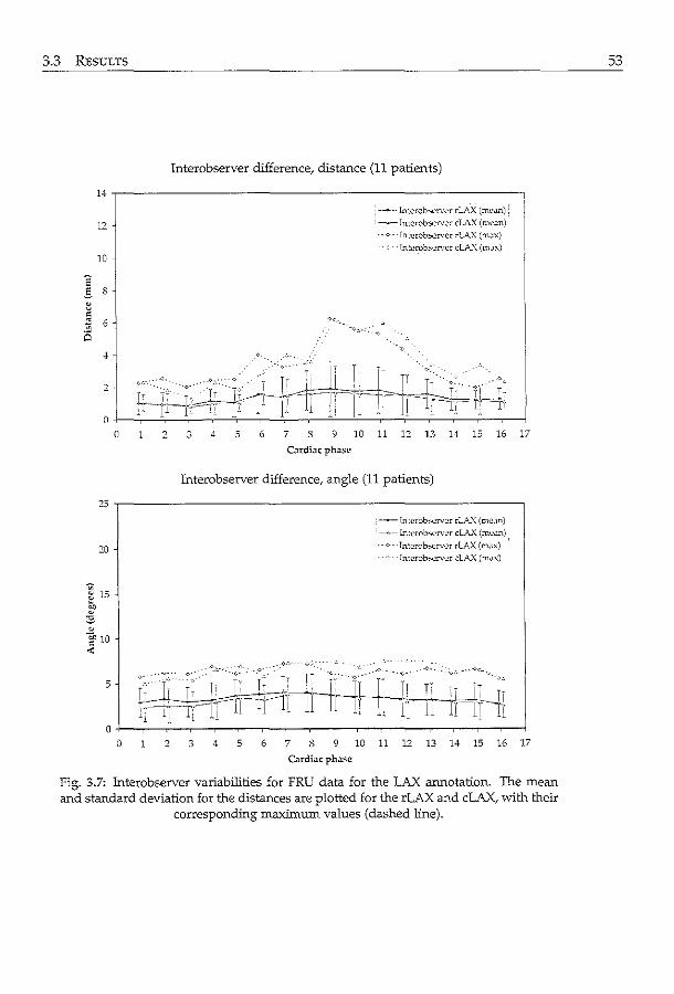
3.3 RESULTS

Interobserver difference; distance (11 patients)

14

-<>--lntcrob~rv<:r rL\..'\ {mc<tn)

12 --ln!<.'rob,;erwr cLAX (ml'.m)

-- v- lnL-crOb'-""'rvcr rLAX (mJ.x)

lntcrobo;ervcr cLA.'\ (m.lx) 10

~ s ~ = " 6 a

4

2

0 0 2 3 4 5 6 7 8 9 10 11 12 13 14 15 16 17

Cardiac phase

Interobserver difference, angle (11 patients)

25

--lntcrob-,;ervcr rLA.'\ (m..:.:~n}

--Interob'-""'rvcr cLA..X (mc.m)

20 ---<--- lntcrob"'-'rvl'r rlAX (mJx) Intcrob,..,rver clAX (m,.,x)

. 0 15 0

['

"' 0

~ 10 .:;:

5

0 0 2 3 4 5 6 7 8 9 10 11 u 13 14 15 16 17

Cardiac ph.lsc

Fig. 3.7: Interobserver variabilities for FRU data for the LAX annotation. The mean and standard deviation for the distances are plotted for the rLAX and cLAX, with their

correspondffig maximum values (dashed line).

53

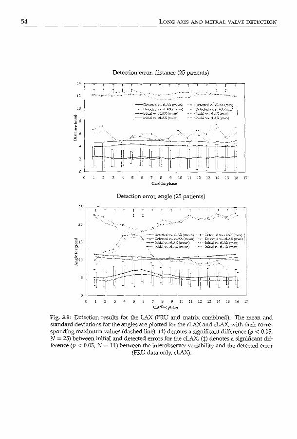
54

14

12

10

'E .§ 8

" 0

' ~ 6

4

2

0

0 '

20

5

LONG AXIS AND MITRAL VALVE DETECTION

Detection error, distance (25 patients)

3 4

--Ddc•ctc·d y,_ rlAX (me~n) ~ Dc•tc•clc'd "'· cLAX (mc•~n)

, -- Initi~l v~. rL'I.X (mc~n) --+--- Inltbl V>. cLA..X (mcilll)

_,._ .~:·.- .

---o- .. . ..,::··

i' 5 6 7 8 9 10

Cardiac ph<tSc

.

]]

· Dckcted v~. rLAX (m~x) DC'tc•ctc>d ,.,._ cLA.."\ (m.cx)

· Iruti.11 v~. rLAX (mux) -Inltbl v,.. cLA...X (m.:c")

' '·

,. 11

r--~r~ li 1! j j.

12 13 14 15 16

Detection error, angle (25 patients)

•• ·o- -lktccted v,. rLA .. '\ (mc·~n) .. .,. · · D<:tc·cted ""- rlAX (m.1x) :, -~ O..•R•ctc•d v.,_ clAX (mwn) O..•tc•ctc•d v"- cLAX (m~x) · -•- Wtbl ""· rl:\..'\ (m<'.m) ·- Initl~l v>. ~LA..'\ (max}

-Jniti.1l V>. cLAX (mc•un) lniti.1l V'- rlA..'\ (m.lx)

17

O·L-----------------------------------------~ 0 .2 3 4 5 7 8 9 10 11 12 13 14 15 16 17

Cardi.1c phase

Fig. 3.8: Detection results for the LAX (FRU and matrix combiDed). The mean and standard deviations for the angles are plotted for the rLAX and cLAX, with their corre­sponding maximum values (dashed line). (t) denotes a significant difference (p < 0.05, N = 25) between initial and detected errors for the cLAX. (:j:) denotes a significant dif­ference (p < 0.05, N = 11) between the interobserver variability and the detected error

(FRU data only, cLAX).

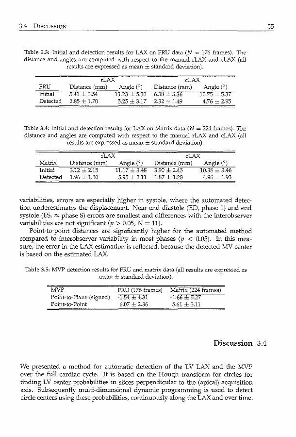
3.4 DISCUSSION

Table 3.3: Initial and detection results for LAX on FRU data (N = 176 frames). The distance and angles are computed with respect to the manual rLAX and cLAX (all

results are expressed as mean ± standard deviation).

rLAX FRU Distance (mm) Initial 5.41 ± 3.54 Detected 2.85 ± 1.70

Angle(') 11.23 ± 5.30 5.25 ± 3.17

cLAX Distance (mm) 6.38 ± 3.36 2.32 + 1.49

Angle(') 10.75 ± 5.37 4.76 ± 2.95

Table 3.4: Initial and detection results for LAX on Matrix data (N = 224 frames). The distance and angles are computed vvith respect to the manual rLAX and cLAX (all

results are expressed as mean ± standard deviation).

Matrix Initial Detected

rLAX Distance (mm) 3.12 ± 2.15 1.96 -'- 1.30

Angle(') 11.17 .:._ 3.48 5.95 ± 2.11

cLAX Distance (mm) 3.90 ± 2.45 1.87 ± 1.28

Angle(') 10.38 ± 3.46 4.96 ± 1.93

variabilities, errors are especially higher in systole, where the automated detec­tion underestimates the displacement. Near end diastole (ED, phase 1) and end systole (ES, "" phase 8) errors are smallest and differences with the interobserver variabilities are not significant (p > 0.05, N = 11).

Point-to-point distances are significantly higher for the automated method compared to interobserver variability in most phases (p < 0.05). In this mea­sure, the error in the LAX estimation is reflected, because the detected MV center is based on the estimated LAX.

Table 3.5: MVP detection results for FRU and matrix data (all results are expressed as mean ± standard deviation).

MVP Point-to-Plane (signed) Point-to-Point

FRU (176 frames) -1.54 ± 4.31 6.07 ± 2.36

Matrix (??4 frames) -1.66 = 5.27 5.61 ± 3.11

Discussion 3.4

We presented a method for automatic detection of the LV LAX and the MVP over the full cardiac cycle. It is based on the Hough transform for circles for finding LV center probabilities in slices perpendicular to the (apical) acquisition axis. Subsequently multi-dimensional dynamic programming is used to detect circle centers using these probabilities, continuously along the LAX and over time.

55

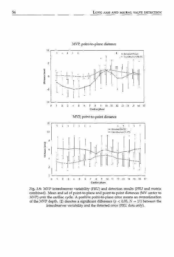
56 LONG AXIS AND MITRAL VALVE DETECTION

MVP, point-to-plane distance

10 ,-----------------------------------------, --- Ddc'Ctc'CI (N~:!.J) ....,_ Int<.'rob,._•n•c•r (N•ll)

5

-5

-10 '-------------------------------------__J

12

10

2

0 2 3 -t 5 6 7 8 9 JO 11 12 13 14 15 16 17

C.u:di:~c ph<:~se

MVP, point-to-point distance

--- D<'lect<.'\':1 (N~:S) -~-rn~rob_..._.,,.r (:"J~11)

2 3 5 6 7 8 9 10 11 12 13 14 15 16 17

C:rrdiJc pha~c

fig. 3.9: MVP interobserver variability (FRU) and detection results (FRU and matrix combined). Mean and sd of point-to-plane and point-to-point distances (MV center to MVP) over the cardiac cycle. A positive point-to-plane error means an overestimation of the MVP depth. (:f) denotes a significant difference (p < 0.05, N = 11) between the

interobserver variability and the detected error (FRU data only).

3.4 DISCUSSION

We employ least squared distance line fit to find the LAX in each cardiac phase. The MVP is located using the detected LAX in a spherical projection, using low­level edge detection by dynamic programming.

The method consists of a few consecutive steps. After determination of LV center, probabilities using HT, on integrated slices of the volume, MDP in 3D results in continuous LV center probabilities and serves as outlier removal for the LV center probability. The same holds for MDP over time. In this way, all available data is combined and a robust continuous detection is achieved.

With respect to the initial LAX errors, the method shows significant improve­ment, with maximum distance errors of 6.07mm in ED and 5.07mm in ES, and angle errors of 8.80 for ED and 8.75 for ES (all for the cLAX). These maximum errors indicate the usability of the LAX detection as an initialization step, espe­cially when taken into account that ED and ES are the most important cardiac phases for initialization of automated procedures, because they represent the two geometrically extreme states of the LV Moreover, LAX detection did not show significant differences with respect to our interobserver variabilities, whlch were achleved in the idealized situation where both observers agreed on endocardial border tracing conventions in advance. In daily clinical situations, these observer variabilities are expected to be considerably larger.

In the analysis of the interobserver variabilities and the detection errors, we normalized the patients' cardiac cycles to 16-phases cycle. In this normalization the position of the ES-phase has not been taken into account due to small variation in the duration of systole among the patients. Therefore, in the analysis shown in Fig. 3.8 and Fig. 3.9 there is no cardiac phase that can be depicted as ES. Instead, ES has been faded over a few cardiac phases.

The detection of the MVP depends on the detection of LAX. This may influence automatic location of the MVP in patients suffering from pathologies that alter the LV shape considerably. The method may be extended by applying same kind of quality control or reliability estimate, e.g. by using the quality of the final line fit in estimating the LAX per cardiac phase. Nevertheless, a small deviation of the LAX from its true position, does not affect the MVP detection much. Thls is because the mitral valve is approximately a planar structure, almost perpendicular to the LAX. The detection of the MVP is limited to finding a MVP plane perpendicular to the LAX, while the true MVP usually is not located exactly perpendicular to the LAX. We found deviations of 5.18 ± 2.81 degrees (mean± sd) from the plane perpendicular to the LAX (N = 400 frames) in our manual tracings. These small differences may be discarded for our initialization purposes.

Automatic initialization of segmentation of the LV in 3DE decreases analysis time for assessment of LV function drastically. Moreover, it eliminates observer variability and therefore makes measurements more reproducible and therefore allows inter-institutional comparison of LV function assessments. Thls is of great value for large studies, for example in clinical trials. However, it of course remains to be proven that such automated measurements, employing a combination of automated analysis and detection, is accurate in comparison to the gold standard.

The presented method provides a basis for localization of LV salient structures, as has been illustrated by the detection of the MVP. Given the location and ori-

57

58 LONG AXIS AND MITRAL VALVE DETECTION

entation of these landmarks one can estimate the complete orientation of the LV using the knowledge of the acquisition to determine the angle of the right ventri­cle (RV) with respect to the LAX. Thls makes it a suitable method for initialization of subsequent processing steps, such as LV segmentation.

As a complete initialization approach for LV segmentation, the proposed method lacks true apex detection. Thls should not be seen as an important short­coming of the method. We expect that initialization can be done reliably using the LAX and MVP. The remaining freedom in the LV position and orientation is very limited, and final determination of this position, orientation and shape should be treated by the segmentation approach.

3.4.1 Study setup

In our experiments we evaluated the LAX and MVP detection on data from pa­tients with various diagnoses of cardiovascular disease. In this population the method showed robustness combined with good accuracy. Although patient data was used for evaluation, the method might encounter problems in very patholog­ical cases showing aberrant LV shapes (e.g. apical aneurysms). These topics need to be further investigated. Note however, that the definition of the LV LAX in these cases also is problematic. Largest errors in the LAX detection in our study (which accounted for the maximum angle errors in systole, Fig. 3.8) were caused by one patient with a highly trabeculated ventricle, which misled the LV center detection. Thls would be a subject for further research on LAX detection.

The application to patient subpopulations, such as patients with an extremely dilated LV probably requires adjustments of the method's parameters concerning the expected LV diameter (rmax)-

In this study, because of the limited availability of patient data, the same data sets were used for parameter training (optimization) as for testing, while ideally these data sets should be different. However, the parameter optimizations have shown that parameter choices are not very critical, because of the very small gain in performance during the second, dependent, parameter optimization. In this optimization, where the optimum neighboring parameter space has been fully explored, in 80% of the evaluations the objective metric was less than 12% above the optimum. Thls range is small compared to the initial estimation where the objective metric is 96% higher. Also, differences in optimal parameters between the two acquisition methods were small. In an evaluation of the LAX detection on FRU and matrix data with the mean of the individually optimized parameters (Table 3.2), the objective metric deviated less than 1% from the optimal case. For these reasons, very similar results can be expected if the training set is separated from the test set.

3.4.2 Performance of matrix vs. FRU data

The initial distance errors for the LAX are lower for the matrix acquisitions. Thls can be attributed to the difference in the acquisition procedure. For the matrix system, a bi-plane view is shown when positioning the probe. For the FRU acqui-

3.4 DISCUSSION

sitions, the sonographer currently needs to alter between the two planes, which makes positioning slightly more difficult. This is reflected in the higher initial distance errors for the FRU data.

Automatic detection yields very similar performance for the two acquisition types. The differences in distance and angle errors between them were not sig­nllicant (p > 0.05). Detections on matrix data show lower distance errors, while detections on FRU data show a slightly lower angle error. These differences are small and might be due to differences in the patient populations.

59

Hough transform for circles 3.4.3

The analysis of the LV in planes perpendicular to the acquisition axis assumes a circular shape of the myocardium in these planes. This is an important assump­tion in the estimation of the LV centers using the Hough transform for circles. However, either due to deviation from the true short-axis angle (in fact we are trying to detect this angle) or due to the left ventricular shape, the LV may appear like an ellipse in the images in which the LV center is detected. As a consequence, one might argue that a Hough transform for ellipses would be more appropriate when detecting the LV center. A disadvantage of a Hough transform for ellipses would be that two extra parameters must be estimated, namely the minor radius and the rotation angle of the ellipse. This would make the detection computa­tionally more expensive. The same holds for the possible extension of the Hough transform to 3D for detecting ellipsoids.

In practice, the HT c will also be capable of approximating centers of ellipses with arbitrary minor radius and orientation, as long as the major and minor ra­dius are close to, or within the accepted range of the radius for the HT,. Also, the actual deviation of the planes perpendicular to the acquisition axis from the true short-axis planes is limited as the initial errors show (Table 3.3 and 3.4), because in the acquisition the sonographer aims at aligning the acquisition axis to the LV LAX.

LV apex detection and LAX length 3.4.4

In the detection of the MVP, the projected endocardial border is detected using the radial gradient in a spherical projection. This border is used to find the MVP. Similarly, the apex could be detected for computation of the LAX length. The highest point of the detected border, or the intersection of this border with the LAX could be used as estimation for the LV apex. A drawback of such an apex detection is that it is very sensitive to the initially detected LAX. A small deviation of the LAX from its true position leads to a considerably lower intersection of the LAX with the endocardial border, especially when the ventricle is narrow near the apex, resulting in a misplaced apex and an underestimation of the LAX length. Furthermore, the presence of near field artifacts in the image obscures the apical region in the projection image. This complicates the detection of the apex in these images using a low-level border detection technique. Therefore, we leave the task of detecting the apex to the proper segmentation method.

60 LONG AXIS AND MITRAL VALVE DETECTION

3.4.5 Extensions

The presented method detects the LV LAX, and using this LAX, also the MVP. Once the LAX is defined, a multitude of possibilities for detecting other salient structures may become feasible. One of the most desirable structures may be the right ventricle (RV), or more specifically, the RV attachment points. This would allow full determination of the position of the LV in 30, with respect to all six degrees of freedom (translation and rotation). The presented method leaves the rotation around the LAX (z-rotation) unattended. Note however, that the variation in z-rotation is limited, because acquisitions are made using the 2- and 4-chamber view as a reference. The detection of the RV in data from current 30E scanners is problematic, because in many regular acquisitions the RV is hardly visible. The (inferior) RV attachment point is visible in most cases, but the occasional absence of this point and the presence of image artifacts that may fool the detection, mak­ing it a feature that is hard to locate fully automatically. When feature detection is used for automatic initialization purposes, such failures are very undesirable.

Currently, we detect the level of the MVP with respect to the LAX. This serves its goal as an initialization for segmentation of the LV. A desirable extension of the method may be automatic detection and tracking of the MV hinge points. The mitral annular motion is useful in the evaluation of global and regional LV function and an important parameter in the diagnosis of annular diseases and LV disorders [Eto et a!., 2005; Pai et a!., 1991; Willenheimer et a!., 1999]. The hinge points are typically visible as bright structures and seem suitable for automated detection. Automated tracking of these points has been shown to be feasible in 20 echocardiography by Nevo eta!. [2007].

3.4.6 Computational costs

For initialization methods, low computational costs are obviously desirable. The detection of the LV LAX and MVP over the full cardiac cycle (16 phases) took two to four minutes on a regular PC (Intel Pentium IV, 2.6 GHz), depending on pa­rameter choices. The implementation of the method (in C++) was not optimized for speed and is suitable for parallel processing. Furthermore, the method may be considerably sped up by applying it at a lower resolution because of the coarse nature of the desired feature detection. Besides, the optimization of the method's parameters shows that parameter choices are not very critical. This gives room for parameter choices that increase performance in terms of computational costs, without noticeably decreasing the accuracy of the method.

3.5 Conclusions

We presented a method for automatic detection of the LV LAX and the MVP over the full cardiac cycle. It is based on a Hough transform for circles and multidi­mensional dynamic programming for detecting the LV LAX continuously over the

3.5 CoNCLUSIONS

cardiac cycle in 3DE. Using the detected LAX, it locates the MVP by employing a DP border detection in a spherical projection of the 3D LV. In an evaluation on FRU and matrix data, the method has shown to be robust and accurate in detect­ing the LAX and MVP. The accuracy, combined with its low computational costs, make it very suitable for initialization purposes for automated segmentation al­gorithms for the LV.

Acknowledgments

This study was funded by the Dutch innovation-oriented research programs (IOP, IBVC02003).

61

Rest-to-stress registration for 3D stress echocardiography 3D stress echocardiography is a novel technique for diagnosing cardiac dysfunction. It involves evaluating wall motion of the left ventricle, by visually analyzing ultrasound images obtained in rest and in different stages of stress. Since the acquisitions are performed minutes apart, variabilities may exist in the visualized cross-sections. To improve anatomical correspondence betvveen rest and stress, alignillg the images is essential. We developed a new intensity-based, sparse registration method to retrieve standard anatomical views from 3D stress images that were equivalent to the manually selected views in the rest images. Using sparse image planes, the influence of common image artifacts could be reduced. We investigated different similarity measures and different levels of sparsity. The registration was tested using data of 20 patients and quantitatively evaluated baSed on manually defined anatomical landmarks. Align­ment was best using sparse registration with tvvo long-axis and tvvo short-axis views; registration errors were reduced significantly, approaching the interobserver variabil­ities. In 91% of the cases, the registration result was qualitatively assessed as better than or equal to the manual alignment. In conclusion, sparse registration improves the alignment of rest and stress images, with a performance similar to manual alignment. This is an important step toward objective quantification in 3D stress echocardiogra­phy.

@2008 IEEE. Reprinted, with pcnni'l.'>ion, from: Sp.:u:sc Rcgistr.ltion for Three-Dimensional Stress Echocaxdiogr.tphy K Y.E. Leung. M. vm Str.:Uen, A. Nemes, MM. Vootmolen, G. vm Burkcn, M.L Gel("ijnsl', F.J. tm Cat(",J.H.C. Reiber, K. de Jong. AF.W. v.m dcr St~n, and J.G. Bo~ IEEE Trans Med Imag 2008; 27(11); 1568-79.

64 REST-TO-STRESS REGISTRATION

4.1 Introduction

4.1.1 Three-dimensional stress echocardiography

Cardiovascular diseases are a major cause of death in the western world. A commonly used method for detecting myocardial dysfunction and underlying coronary artery disease is stress echocardiography [Armstrong and Zoghbi, 2005; Marwick, 2003; Matsumura et al., 2005; Yang et al., 2006; Zwas et al., 1999]. This technique is used to evaluate wall motion of the left ventricle (LV), usually by visual examination of ultrasound images that are obtained in rest and in differ­ent stages of exercise or pharmacological stress. Recent advances in real-time 3D echocardiography [Caiani et al., 2005; Jenkins et al., 2006] show great potential in overcoming major limitations of traditional 2D stress echocardiography, such as variabilities in the visualized LV cross-sections and high subjectivity of visual wall-motion scoring. Our long-term goal is to develop more objective and quanti­tative analysis methods for 3D stress echocardiography, by automating the image analysis.

We have decided to tackle the automation in tluee steps: 1) alignment of im­ages acquired in rest and in stress stages, 2) segmentation of the myocardial wall and quantification of wall motion, and 3) automatic classification of wall-motion abnormalities. This chapter describes the first step. The alignment of the rest and stress images is necessary because the rest and stress images are acquired several minutes apart. Therefore, variations may exist in the visualized cross-sections of the LV [Ahmad et al., 2001]. Possible sources of misalignment between rest and stress are placement and tilting of the ultrasound probe, as well as patient breathing [Shekhar et al., 2004], both of which may lead to inaccuracies when comparing wall motion in the rest and stress stages. We start with image align­ment for two reasons. First, registration will greatly assist the segmentation of the myocardial wall by providing a high-quality initialization for the segmentation in the rest image [Pickard et al., 2005; Walirnbe et al., 2006; Zagrodsky et al., 2005] or the stress image. Second, misalignment will impair the diagnostic quality of the wall-motion differences found in rest and stress, whether by visual scoring or by automatic segmentation. Registration will improve the anatomical correspon­dence of the LV segments, resulting in a better-quality wall-motion comparison between rest and stress.

4!.1.2 Registration research and related work

Intensity-based image registration is widely used for aligning two or more im­ages [Hill et al., 2001; Maintz and Viergever, 1998; Makela et al., 2002; Pluim et al., 2003]. Although most registration work is performed on computed tomogra­phy (CT) and magnetic resonance (MR) images, ultrasound image registration has gained considerable interest in recent years [Pluim and Fitzpatrick, 2003]. Among the early examples of 3D ultrasound intensity-based registration are spatial com-

4.1 INTRODUCTION

pounding of gall bladder images [Rohling et al., 1998] and registration of breast images [Kroeker et al., 2000; Meyer et al., 1999]. More recent examples include registration of liver images using attribute vectors [Foroughi and Abolmaesumi, 2006] and tracking brain deformations in intraoperative time series [Pennec et al., 2003]. Registration of ultrasound images with images from other modalities has also been investigated. For example, ultrasound to CT registration was explored by Penney et al. [2006] for alignment of images of the femur and pelvis. Ultra­sound to MR registration is mairly used in the context of aligning intraoperative ultrasound images to preoperative MR images of e.g., the liver [Penney et al., 2004] and the brain [Letteboer et al., 2005; Roche et al., 2001].

Several papers have been published recently on 2D and 3D ultrasound car­diac registration. Using a phase-based similarity measure, Grau et al. registered 3D images acquired from the parastemal and the apical echocardiographic win­dows [Grau and Noble, 2005; Grau et al., 2006]. A similar approach was used by Zhang et al. [2006] to register 3D cardiac ultrasound images to 2D MR images. Nonrigid registration with spatial and temporal constraints has been proposed to determine cardiac motion in 2D ultrasound sequences [Ledesma-Carbayo et al., 2006, 2005]. In the cardiac domain, registration of ultrasound and single photon emission computed tomography (SPECT) images was described by Walimbe et al. [2003].

Registration of rest and stress images has also been investigated. To study differences in myocardial perfusion between rest and stress, Declerck et al. [1997] registered SPECT images by aligning myocardial feature points with an adapted iterative closest point algorithm. Delzescaux et al. [2003] used a surface-based registration algorithm involving geometrical models of the left and right ventricles to align rest and stress MR images. An intensity-based approach using rest and stress templates was proposed by Slomka et al. [1995] for SPECT images. This method was later augmented with an intensity normalization factor, to account for differences in doses and isotopes used between rest and stress [Slomka et al., 2004]. More recently, Juslin et al. [2007] studied registration with the mutual information metric to PET images. Independent component analysis was applied to the images before registration to extract the voxels representing cardiac tissues.

Closely related to this chapter is the work of Shekhar et al. on registration of cardiac ultrasound 3D images, either in the same time sequence [Shekhar and Zagrodsky, 2002] or in rest and in stress [Shekhar et al., 2004]. Rigid and affine registration using the mutual information similarity measure was investigated. The approach was also used as a first step in cardiac segmentation by Zagrodsky et al. [2005] and Walimbe et al. [2006]. However, this full-3D registration method was evaluated only qualitatively.

65

Sparse registration 4.1.3

In this chapter, a new method was developed to align rest and stress images. The key feature of this method is sparsity: only anatomical four-chamber, two­chamber, and short-axis planes of the rest image are used for the registration. A big advantage of using only sparse image information is that it allows us to define

66 REST-TO-STRESS REGISTRATION

the structures contributing most to correct alignment explicitly. In practice, these anatomical views are usually the starting point for further visual assessment of cardiac motion. Selecting and aligning these rest and stress views consistently are therefore essential steps in wall-motion comparison. An additional advantage of using only sparse views for registration is that the influence of common ul­trasound anomalies, such as near-field artifacts and echo reverberations, can be limited. These artifacts can dominate large regions of the image, which distort the calculation of the registration metric. Furthermore, less computation effort is needed than in full-3D registration.

The focus on sparsity and the quantitative evaluation using a manual gold standard distinguishes this study from the work of Shekhar et a!. [2004], who investigated full-3D mutual-information registration. Our method bears more resemblance to the slice-to-volume registration as reported by Fei et a!. [2003], rather than to the 3D to 2D registration methods where 2D projections of the 3D image are registered in 2D [Penney et al., 1998].

To reduce the variability in visualized cross-sections in 3D stress echocardio­graphy, an intensity-based, sparse registration method was used to retrieve four­chamber, two-chamber, and short-axis views from 3D stress images that were equivalent to the manually selected views in the rest images. The focus is on spatial alignment of 3D rest and stress images, rather than temporal alignment within a single time-sequence. Four similarity measures, the level of sparsity, and optimal resolution levels were investigated. The registration was evaluated quan­titatively using 20 end-diastolic and end-systolic patient data sets, with manually annotated points as the gold standard. The registration results were compared with interobserver and intraobserver variabilities in manual alignment. A visual, qualitative assessment of the registration performance was also performed.

4.2 Methods

The alignment of rest and stress images was accomplished as follows. First, the anatomical coordinate system, which consists of the major axis (i.e., long axis) of the left ventricle (LV) and the direction of the four-chamber view, was manually defined in the 3D rest image. Next, the four-chamber (4C), two-chamber (2C), and short-axis (SAX) views were constructed on the basis of this coordinate system. These are standard anatomical views used in echocardiography [Cerqueira eta!., 2002]. Finally, these anatomical views were automatically registered to the 3D stress image, thus providing the anatomical coordinates in the stress stage. The registration was denoted as sparse, because only the voxels on these anatomical views contributed to the metric calculation. We tested different levels of sparsity by varying the number of SAX planes. The sparse registration was compared with full-3D registration that used all voxels in the 3D image.

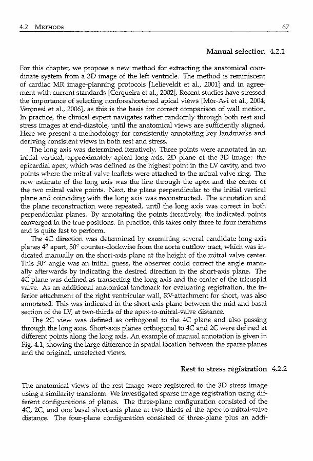
4.2 METHODS 67

Manual selection 4.2.1

For this chapter, we propose a new method for extracting the anatomical coor­dinate system from a 3D image of the left ventricle. The method is reminiscent of cardiac MR image-planning protocols [Lelieveldt et al., 2001] and in agree­ment with current standards [Cerqueira et al., 2002]. Recent studies have stressed the importance of selecting nonforeshortened apical views [Mor-Avi et al., 2004; Veronesi et al., 2006], as this is the basis for correct comparison of wall motion. In practice, the clinical expert navigates rather randomly through both rest and stress images at end-diastole, until the anatomical views are sufficiently aligned. Here we present a methodology for consistently annotating key landmarks and deriving consistent views in both rest and stress.

The long axis was determined iteratively. Three points were annotated in an initial vertical, approximately apical long-axis, 2D plane of the 3D image: the epicardial apex, which was defined as the highest point in the LV cavity, and two points where the mitral valve leaflets were attached to the mitral valve ring. The new estimate of the long axis was the line through the apex and the center of the two mitral valve points. Next, the plane perpendicular to the initial vertical plane and coinciding with the long axis was reconstructed. The annotation and the plane reconstruction were repeated, until the long axis was correct in both perpendicular planes. By annotating the points iteratively, the indicated points converged in the true positions. In practice, this takes only three to four iterations and is quite fast to perform.

The 4C direction was determined by examining several candidate long-axis planes 4 o apart, 50° counter-clockwise from the aorta outflow tract, which was in­dicated manually on the short-axis plane at the height of the mitral valve center. This 50° angle was an initial guess, the observer could correct the angle manu­ally afterwards by indicating the desired direction in the short-axis plane. The 4C plane was defined as transecting the long axis and the center of the tricuspid valve. As an additional anatomical landmark for evaluating registration, the in­ferior attachment of the right ventricular wall, RV-attachment for short, was also annotated. This was indicated in the short-axis plane between the mid and basal section of the LV, at two-thirds of the apex-to-mitral-valve distance.

The 2C view was defined as orthogonal to the 4C plane and also passing through the long axis. Short-axis planes orthogonal to 4C and 2C were defined at different points along the long axis. An example of manual annotation is given in Fig. 4.1, showing the large difference in spatial location between the sparse planes and the original, unselected views.

Rest to stress registration 4.2.2

The anatomical views of the rest image were registered to the 3D stress image using a similarity transform. We investigated sparse image registration using dif­ferent configurations of planes. The three-plane configuration consisted of the 4C, 2C, and one basal short-axis plane at two-thirds of the apex-to-mitral-valve distance. The four-plane configuration consisted of three-plane plus an addi-

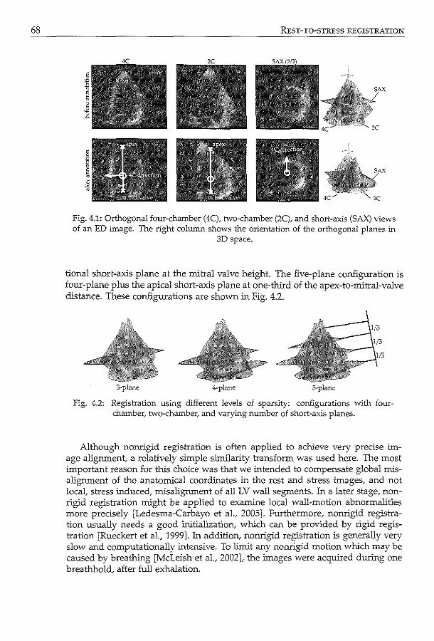
68 REsT-TO-STREss REGISTRATION

4C"'" 2C

Fig. 4.1: Orthogonal four-chamber (4C), two-chamber (2C), and short-axis (SAX) views of an ED image. The right column shows the orientation of the orthogonal planes in

3D space.

tional short-axis plane at the mitral valve height. The five-plane configuration is four-plane plus the apical short-axis plane at one-third of the apex-to-mitral-valve distance. These configurations are shown in Fig. 4.2.

3-pl.me 4-plane

Fig. 4.2: Registration using different levels of sparsity: configurations vvith four­chamber, two-chamber,. and varying number of short-axis planes.

Although nonrigid registration is often applied to achieve very precise im­age alignment, a relatively simple similarity transform was used here. The most important reason for this choice was that we intended to compensate global mis­alignment of the anatomical coordinates in the rest and stress images, and not local, stress induced, misalignment of all LV wall segments. In a later stage, non­rigid registration might be applied to examine local wall-motion abnormalities more precisely [Ledesma-Carbayo et al., 2005]. Furthermore, nonrigid registra­tion usually needs a good initialization, which can be provided by rigid regis­tration [Rueckert et al., 1999]. In addition, nonrigid registration is generally very slow and computationally intensive. To limit any nonrigid motion which may be caused by breathing [McLeish et al., 2002]. the images were acquired during one breathhold, after full exhalation.

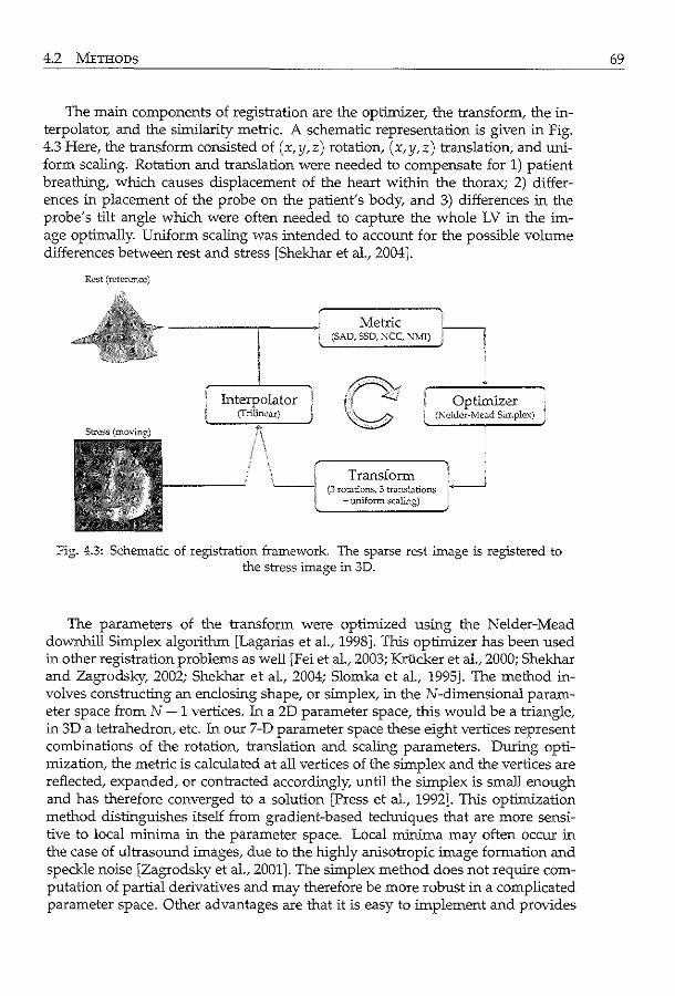
4.2 METHODS

The main components of registration are the optimizer, the transform, the in­terpolator, and the similarity metric. A schematic representation is given in Fig. 4.3 Here, the transform consisted of (x, y,z) rotation, (x, y,z) translation, and uni­form scaling. Rotation and translation were needed to compensate for 1) patient breathing, which causes displacement of the heart within the thorax; 2) differ­ences in placement of the probe on the patient's body, and 3) differences in the probe's tilt angle which were often needed to capture the whole LV in the im­age optimally. Uniform scaling was intended to account for the possible volume differences between rest and stress [Shekhar et al., 2004].

Rest (reference)

Metric i (SAD, SSD, :-.ICC, Nlv!I) 'I

/0:f Optimizer

~ i (Kcldcr-:vfead Simplex)

Transform (3 rotations, 3 transl;:~tions

.,.. uniform scJ.ilng)

fig. 4.3: Schematic of registration framework The sparse rest image is registered to the stress image in 3D.

The parameters of the transform were optimized using the Nelder-Mead downhill Simplex algorithm [Lagarias et al., 1998]. This optimizer has been used in other registration problems as well [Fei et al., 2003; Kriicker et al., 2000; Shekhar and Zagrodsky, 2002; Shekhar et al., 2004; Slomka et al, 1995]. The method in­volves constructing an enclosing shape, or simplex, in the N-clirnensional param­eter space from N + 1 vertices. In a 2D parameter space, this would be a triangle, in 3D a tetrahedron, etc. In our 7-D parameter space these eight vertices represent combinations of the rotation, translation and scaling parameters. During opti­mization, the metric is calculated at all vertices of the simplex and the vertices are reflected, expanded, or contracted accordingly, until the simplex is small enough and has therefore converged to a solution [Press et al., 1992]. This optimization method distinguishes itself from gradient-based techniques that are more sensi­tive to local minima in the parameter space. Local minima may often occur in the case of ultrasound images, due to the highly anisotropic image formation and speckle noise [Zagrodsky et al., 2001]. The simplex method does not require com­putation of partial derivatives and may therefore be more robust in a complicated parameter space. Other advantages are that it is easy to implement and provides

69

70 REsT-TO-STRESS REGISTRATION

a good compromise between robustness and convergence time [Zagrodsky et al., 2001].

Normalized parameters were used during optimization in simplex space. One unit simplex parameter corresponded to 1.1mm translation, 0.4° (x,y) rotation, 0.5° z rotation, and 0.7% scaling. The parameters' normalization factors were determined on the basis of the physical displacement of the image voxel furthest away from the origin of the transform. As an example, an x rotation of 0.4 ° performed on the voxel furthest away from the rotation origin, i.e., in the lowest corner of the image, will lead to a physical displacement of 1.1mm (calculated on a typical data set of 160 x 144 x 208 voxels of 1.mm x 1.1mm x 0.7mm). To correct for the tilt angle of the ultrasound probe easily, the center of the transducer was chosen as the origin of rotation. To preserve the position of the LV as much as possible, the origin of scaling coincided with the center of the image. The initial size of the simplex was 3 units along each parameter axis. Registration was considered to be converged when the simplex hypervolume was smaller than 0.01 and when the differences in metric value at the simplex vertices were less than 10-4 . Trilinear interpolation was used because of computational efficiency.

In our sparse registration setup, we tested several similarity metrics which are commonly used in registration [Giachetti, 2000; Hill et al., 2001; Makela et al., 2002]: sum-of-absolute-differences (SAD), sum-of-squared-differences (SSD), normalized cross correlation (NCC), and normalized mutual information (NMI). NMI was calculated with the histogram method [Maes et al., 1997]. A btn size of 2 was used for the 8-bit data; this was found empirically. Voxels outside the transducer's scan sector did not contribute to the metric calculation. Registration was carried out on four separate resolution levels of a Gaussian image pyramid [Burt and Adelson, 1983]; from full resolution at level 0 to 8 times downsampled at level 3. A multiresolution scheme was also tested.

The sparse image grid was initialized in the stress image, at the same spatial coordinates as the rest image. At each registration iteration, the spatial transform was applied to the coordinates of the sparse rest-image grid. The stress image was then resampled at those coordinates using trilinear interpolation. The metric was calculated using only the voxels on the sparse grid. In this manner, anoma­lies such as near-field artifacts and echo reverberations, which may dominate the metric calculation, could be avoided as much as possible.

4.2.3 Data description and algorithm evaluation

Full-cycle 3D data sets were acquired at the Thoraxcenter (Erasmus MC, Rotter­dam, The Netherlands) on 20 patients in sinus rhythm with chest patn referred for stress testing. A Dobutarnine-Atropine stress protocol was used [Nemes et al., 2007b]. All data sets were obtained in the apical position; each image se­quence was obtained during one breathhold. Patients were imaged at rest and at peak-dose. The data sets for three patients were acquired with the Fast Rotat­ing Ultrasound transducer [Voormolen et al., 2006] developed at the department of Biomedical Engineering (Thoraxcenter, Erasmus MC, Rotterdam, The Nether­lands). The spatial dimension of the images were 128 x 128 x 388, at 1.4 x 1.4

4.2 METHODS

x 0.3mm (length x width x depth). The remaining 17 patients were examined using the commercially available Philips Sonos 7500 machlne equipped with the X4 matrix-array transducer (both from Philips Medical Systems, Andover, MA). These images contained 160 x 144 x 208 voxels of 1.1 x 1.1 x 0.7mm. Reg­istration was tested on 3D rest-and-stress image pairs at end-diastole (ED) and end-systole (ES) separately, because the left ventricle may move differently un­der stress conditions. We chose to evaluate the registration on ED and ES time points because these could be clearly identified for each sequence. ED and ES time points were defined, respectively, by the ECG R-peak and by the mitral valve opening.

To get an overall idea of image quality, the visibility of the 17 LV wall segments [Cerqueira et al., 2002] was judged visually by an expert observer, blinded from the registration results. Each segment was given a score: 4 = optimal, 3 = good, 2 = moderate, 1 = poor, 0 = invisible [Nemes et al., 2007b ]. This was done for all rest and stress image sequences. The average of the 17 scores was then calculated for each patient.

Interobserver and intraobserver variabilities were also analyzed. Two indepen­dent observers indicated the long axis and 4C direction, as well as the aorta, and the RV-attachment in end-diastole and end-systole. The first observer annotated each data set twice, at an interval of at least one day. The second observer indi­cated 11 rest and 11 stress data sets twice, and the remaining data sets once. The intraobserver variability in the apex, mitral valve center, aorta and RV positions was defined as the average of Euclidean distances between annotated points. The intraobserver variability in the 4C angle was defined as the average of absolute differences in angle. Mean and standard deviations were calculated over all indi­cated data sets. The interobserver variability was defined similarly, as the average of differences in the mean annotation of each observer.

Since we were interested in aligning only the anatomical views, a natural choice of landmarks for quantitative evaluation of the registration were the land­marks on the sparse planes. The following landmarks were chosen because they were adequately salient structures in the images: the apex and mitral valve points, the direction of the four-chamber, the aorta outflow tract, and the posterior at­tachment of the right ventricular wall. Although only these landmarks were evaluated, the rest-to-stress point correspondence of the whole myocardial bor­der should also benefit from a good initial alignment. Further comparison of 3D wall-motion might be hampered if the global anatomical coordinate system was not well defined.

The average over all annotations (three to four per data set) was used as the anatomical coordinate system for the registration, thus providing a gold standard. The registration errors for each image-pair were defined as the point-to-point Eu­clidean distances between the gold standard and the registered landmarks. The initial error was defined as the point-to-point distances between the gold standard and the initial position of the landmarks (the same spatial coordinates as the man­ual annotation in the rest image). The errors were calculated for each anatomical landmark and for each rest-stress image pair separately. The registration error was then compared with the initial error using the paired t-test [Altman, 1997].

71

72 REST-TO-STRESS REGISTRATION

The registration errors were also compared with the interobserver and intraob­server variabilities in manual annotation.

In addition to the quantitative evaluation, a qualitative assessment was per­formed by an independent observer, blinded from the registration results. The observer was presented four-chamber, two-chamber, and short-axis views of 1) the manually annotated rest image, 2) the manually annotated stress image, 3) the stress image before alignment (initialized by the landmarks indicated in the rest image), and 4) the stress image after registration, similar to Fig. 4.4. The observer did not know whether set 3) or set 4) corresponded with images before or after registration. First of all, to determine whether the registration resulted in better rest-to-stress alignment, the observer judged if set 3) or 4) was better aligned with set 1), or if there was no visible difference, or if visual assessment was impossible due to poor image quality. A set was considered better aligned if the position of the long-axis and the direction of the four-chamber view in the stress image showed a better correspondence with the rest image. Second, the ob­server judged whether the set that was selected in the first part of the experiment, was worse, equally, or better aligned with the rest image than the manually indi­cated stress image, again on the basis of the long-axis position and four-chamber view.

4.3 Results

4.3.1 Annotation of landmarks

Two independent observers indicated the apex, the mitral valve, the RV-attach­ment on the short-axis view of the three-plane configuration, the aorta center in the short-axis view at mitral-valve height, and the four-chamber direction. Typ­ically, four three-point annotations were needed to indicate the long-axis cor­rectly in both perpendicular long-axis views. The annotation was carried out in MATLAB® (version 6.5.0, release 13, The Math Works, Inc.), which took a few min­utes per data set. Later, we developed dedicated visualization software in C++. Using this program, the annotation time was reduced to less than half a minute for each 3D image. The interobserver and intraobserver variabilities are shown in Table 4.1. Of the five landmarks, the mitral valve was the easiest to annotate, because it was usually a clear salient structure in the image.

4.3.2 Image quality assessment

Using the image-quality scoring system described in the methods section, we found that the overall image quality was moderate, with a mean score of 2.0 ± 1.0 on a scale of 0 (invisible) to 4 (optimal), averaged over the 20 rest and 20 stress time-sequences. The maximum score was 4, the minimum score was 0.46, and the median was 1.85. Not only the image quality itself, but also the difference

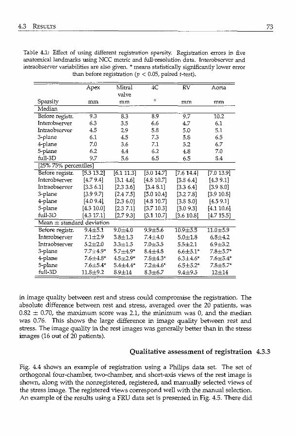
4.3 RESULTS

Table 4.1: Effect of using different registration sparsity. Registration errors in five anatomical landmarks using NCC metric and full-resolution data. Interobserver and intraobserver variabilities are also given. ~·means statistically significantly lower error

than before registration (p < 0.05, paired t-test).

Apex Mitral 4C RV Aorta valve

Sparsity nun nun 0 nun nun Median Before registr. 9.3 8.3 8.9 9.7 10.2 Interobserver 6.3 3.5 6.6 4.7 6.1 Intraobserver 4.5 2.9 5.8 5.0 5.1 3-plane 6.1 4.5 7.3 5.8 6.5 4-plane 7.0 3.6 7.1 5.2 6.7 5-plane 6.2 4.4 6.2 4.8 7.0 full-3D 9.7 5.6 6.5 6.5 8.4 [25% 75% percentiles] Before registr. [5.3 13.2] [6.111.3] [5.0 14.7] [7.6 14.4] [7.0 13.9] Interobserver [4.7 9.4] [3.1 4.6] [4.8 10.7] [3.8 6.4] [4.3 9.1] Intraobserver [3.3 6.1] [2.3 3.6] [3.4 8.1] [3.3 6.4] [3.9 8.0] 3-plane [3.9 9.7] [2.4 7.5] [5.0 10.4] [3.2 7.8] [3.9 10.8] 4-plane [4.0 9.4] [2.3 6.0] [4.8 10.7] [3.8 8.0] [4.5 9.1] 5-plane [4.3 10.0] [2.3 7.1] [3.7 10.3] [3.0 9.3] [4.1 10.6] full-3D [4.317.1] [2.7 9.3] [3.110.7] [3.6 10.8] [4.715.5] Mean ± standard deviation Before registr. 9.4±5.1 9.0±4.0 9.9±5.6 10.9±5.5 11.0±5.9 lnterobserver 7.1±2.9 3.8±1.3 7.4±4.0 5.0±1.8 6.8±4.2 Intraobserver 5.2±2.0 3.3±1.5 7.0±3.5 5.5±2.1 6.9±3.2 3-plane 7.7±4.9* 5.7±4.9* 8.4±4.8 6.6±5.1' 7.8±5.7* 4-plane 7.6±4.8* 4.5±2.9* 7.8±4.3* 6.3±4.6'' 7.6±5.4* 5-plane 7.6±5.4* 5.4±4.4* 7.2±4.6'' 6.5±5.2* 7.8±5.7* full-3D 11.8±9.2 8.9±14 8.3±6.7 9.4±9.5 12±14

in image quality between rest and stress could compromise the registration. The absolute difference between rest and stress, averaged over the 20 patients, was 0.82 ± 0.70, the maximum score was 2.1, the minimum was 0, and the median was 0.76. This shows the large difference in image quality between rest and stress. The image quality in the rest images was generally better than in the stress images (16 out of 20 patients).

73

Qualitative assessment of registration 4.3.3

Fig. 4.4 shows an example of registration using a Philips data set. The set of orthogonal four-chamber, two-chamber, and short-axis views of the rest image is shown, along with the nonregistered, registered, and manually selected views of the stress image. The registered views correspond well with the manual selection. An example of the results using a FRU data set is presented in Fig. 4.5. There did

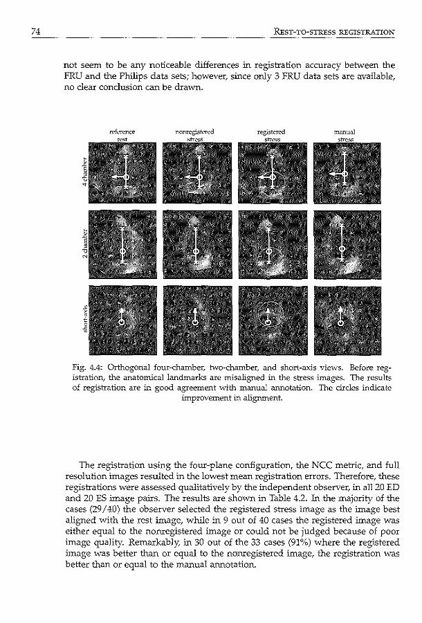
74 REST-TO-STRESS REGISTRATION

not seem to be any noticeable dilierences in registration ac=acy between the FRU and the Philips data sets; however, since only 3 FRU data sets are available, no clear conclusion can be drawn.

Fig. 4.4: Orthogonal four-chamber, two-chamber, and short-axis views. Before reg­istration, the anatomical landmarks are misaligned in the stress images. The results of registration are in good agreement with manual annotation. The circles indicate

improvement in alignment.

The registration using the four-plane configuration, the NCC metric, and full resolution images resulted in the lowest mean registration errors. Therefore, these registrations were assessed qualitatively by the independent observer, in all20 ED and 20 ES image pairs. The results are shown in Table 4.2. In the majority of the cases (29 I 40) the observer selected the registered stress image as the image best aligned with the rest image, while in 9 out of 40 cases the registered image was either equal to the nonregistered image or could not be judged because of poor image quality. Remarkably, in 30 out of the 33 cases (91%) where the registered image was better than or equal to the nonregistered image, the registration was better than or equal to the manual annotation.

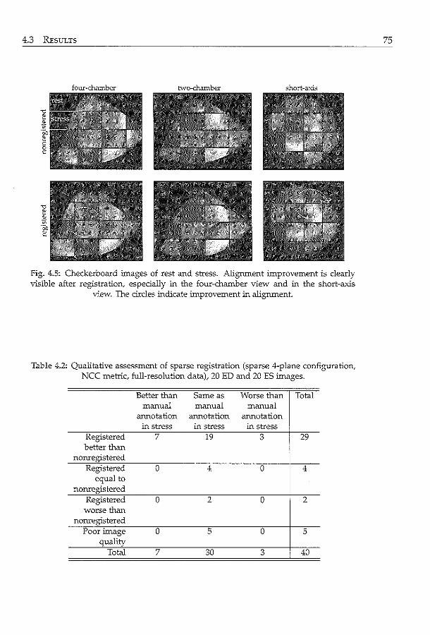
4.3 REsULTS

four~chamber hvo-chamber short-axis

Fig. 4.5: Checkerboard images of rest and stress. Alignment improvement is clearly visible after registration, especially in the four-chamber view and in the short-axis

view. The circles indicate improvement in alignment.

Table 4.2: Qualitative assessment of sparse registration (sparse 4-plane configuration, NCC metric, full-resolution data), 20 ED and 20 ES images.

Better than Same as Worse than Total manual manual manual

annotation annotation annotation in stress in stress in stress

Registered 7 19 3 29 better than

nonregistered Registered 0 4 0 4

equal to nonregistered

Registered 0 2 0 2 worse than

nonregistered Poor image 0 5 0 5

quality Total 7 30 3 40

75

76 REST-TO-STRESS REGISTRATION

4.3.4 Quantitative assessment of registration

Sparsity

Fig. 4.6 and Table 4.1 show the results of registration using the normalized cross­correlation metric and full-resolution data for different levels of sparsity. The registration errors over 20 ED and 20 ES image-pairs are presented for each of the five landmarks. Minimal differences in errors were found between ED and ES image-pairs. Lower median errors were found in most cases, for both sparse and full-3D registration. The 25%-75% percentile range of registration errors is quite close to the interobserver range (Fig. 4.6). 1n particular, the mean errors of the sparse registration with the four-plane configuration were the lowest, and comparable with the interobserver variability (Table 4.1). A closer inspection re­vealed that the mean errors of full-3D were distorted because of outliers of some image pairs (Fig. 4.6). For each landmark, the registration of a rest-stress image pair was considered failed if the registration error was higher than the maximum initial error encountered in all 20 ED and 20 ES image pairs. These maximum initial errors were 18.6mm for the apex, 20.4mm for the mitral valve, 22.8° for the four-chamber direction, 24.6mm for the RV-attachment, and 30.4mm for the aorta.

Although the differences between the different levels of sparsity were small, registration using the four-plane configuration appeared to be most robust (Fig. 4.6). Therefore, we will show registration results using this four-plane configura­tion in the following.

Registration metric

Table 4.3 shows the results of registration with the four-plane configuration, for the SAD, SSD, NCC, and NMI metrics. Registration using the NCC metric im­proved the alignment in all five landmarks statistically significantly.

Image resolution

Table 4.4 shows the registration results for different image resolutions. Registra­tion on full resolution data performed better than registration on downsampled data. We also tested a multiresolution scheme, starting at resolution level 1, and finishing at level 0. 1n 4 out of 40 cases, the registration in level 1 resulted in an outlier for at least one landmark. 1n those cases, further registration on level 0 resulted in minimal improvement. Therefore, these cases were not taken into ac­count in the reported multilevel results. 1n this subset of registration image pairs, minimal differences in results were found between the multilevel approach and the single level 0 approach.

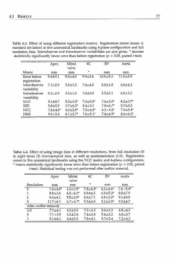
4.3 REsuLTS

Table 4.3: Effect of using different registration metrics. Registration errors (mean ± standard deviation) in five anatomical landmarks usffig 4-plane configuration and full resolution data. Interobserver and intraobserver variabilities are also given. ~· denotes statistically signilicantly lower error than before registration (p < 0.05, paired t-test).

Apex Mitral 4C RV Aorta valve

Metric mm mm 0 mm mm

Error before 9.4±5.1 9.0±4.0 9.9±5.6 10.9±5.5 11.0±5.9 registration Interobserver 7.1±2.9 3.8±1.3 7.4±4.0 5.0±1.8 6.8±4.2 variability Intraobserver 5.2±2.0 3.3±1.5 7.0±3.5 5.5±2.1 6.9x3.2 variability SAD 9.1±5.7 5.3=3.0*• 7.8±5.3'" 7.3±5.0* 8.2±5.7*• SSD 9.8±5.9 5.7±6.2* 8.4±5.1 7.9±6.7* 8.7±8.3 NCC 7.6±4.8'" 4.5±2.9* 7.8±4.3* 6.3±4.6'" 7.6x5.4* NMI 9.0x5.6 6.1±3.7'" 7.6±5.1'" 7.4±4.9'" 8.6±6.3*

Table 4.4: Effect of using image data at different resolutions, from full resolution (O) to eight times (3) downsampled data, as well as multiresolution (1-0). Registration errors in five anatomical landmarks using the NCC metric and 4-plane configuration. * means statistically significantly lower error than before registration (p < 0.05/ paired

t-test). Statistical testing was not performed after outlier removal.

Apex Mitral 4C RV Aorta valve

Resolution mm mm 0 mm mm

0 7.6±4.8* 4.5±2.9* 7.8_:_4.3*• 6.3±4.6'" 7.6±5.4'" 1 8.8±5.6 4.8±4.2* 8.9±6.5 6.9±5.2* 8.8±7.9 2 9.5±6.1 5.5±3.9'" 8.6±7.1 6.9±5.0* 9.1±8.0 3 11.7±6.1 6.7±4.7* 9.5±6.8 8.2±5.8'" 9.5±6.7 After outlier removal 1-0 7.7±4.1 4.3±3.0 7.5±4.3 5.6±3.3 6.8±4.5 0 7.1±3.9 4.2±2.4 7.4±3.8 5.6±3.2 6.8±3.7 1 8.1±4.1 4.4±2.8 7.8±4.1 5.7±3.4 7.2±4.2

77

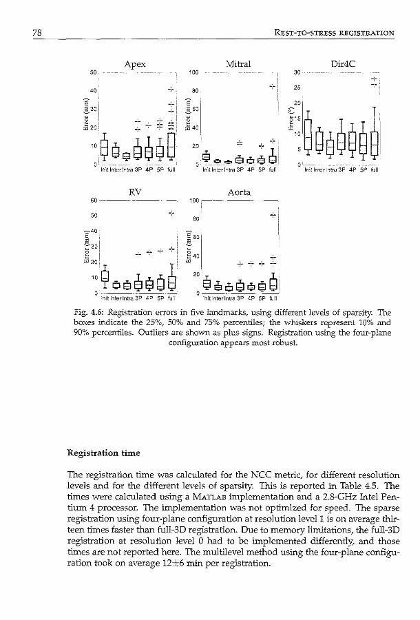
78

Apex 50

40

+ " 8 --_,_--

~::$g~8e~B 0'

lnit Inter Intra 3P 4P SP full

RV 60 ----------·

50

640,

£3o! 5: __ .·.:

;§:::$ oe ~ $ Q ~' 0 -~--------·----·---

lnitlnterlntra 3P 4P SP full

REsT-TO-STRESS REGISTRATION

Mitral Dir4C 100 30

80 25

20

l::~Ge9~~~ 2 ~ 40

20

e ... ..,so .. e~.! 0 - -·---- - - - 0 fn':tlnterlntra 3P 4P SP full !nit Inter Intra 3P 4P SP full

Aorta 1QQ,---~-- --- -

80

.:--:-+--20 ,I, eso~e$~i

0 ------------"--' lnltlnterlntra 3P 4P SP full

Fig. 4.6: Registration errors in five landmarks, using different levels of sparsity. The boxes :indicate the 25%, 50% and 75% percentiles; the whiskers represent 10% and 90% percentiles. Outliers are shown as plus signs. Registration using the four-plane

configuration appears most robust.

Registration time

The registration time was calculated for the NCC metric, for different resolution levels and for the different levels of sparsity. This is reported in Table 4.5. The times were calculated using a MATLAB linplementation and a 2.8-GHz Intel Pen­tium 4 processor. The linplementation was not optimized for speed. The sparse registration using four-plane configuration at resolution Ievell is on average thir­teen times faster than full-3D registration. Due to memory limitations, the full-3D registration at resolution level 0 had to be linplemented differently, and those times are not reported here. The multilevel method using the four-plane configu­ration took on average 12±6 min per registration.

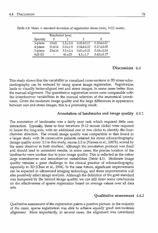
4.4 DISCUSSION

Table 4.5: Mean ± standard deviation of registration times (min)~ NCC metric.

Resolution level Sparsity 0 1 2 3 3-plane 13±8 2.5:t2.8 0.45±0.17 0.15±0.07 4-plane 21±14 3.0±1.9 0.54±0.22 0.17=0.05 5-plane 23±16 3.5±2.4 0.61±0.31 0.18±0.05 full-3D 41±23 4.3±1.7 0.43±0.17

Discussion 4.4

This study shows that the variability in visualized cross-sections in 3D stress echo­cardiography can be reduced by using sparse image registration. Registration leads to visually better-aligned rest and stress images, in some cases better than the manual alignment. The quantitative registration errors were comparable with the interobserver variabilities in the manual selection of the anatomical coordi­nates. Given the moderate image quality and the large differences in appearance between rest and stress images, thls is a promising result.

79

Annotation of landmarks and image quality 4.4.].

The annotation of landmarks was a fairly easy task which required little user interaction. Typically, three to four iterations (9-12 mouse clicks) were required to locate the long-axis, with an additional one or two clicks to identify the four­chamber direction. The overall image quality was comparable to that found in a larger study with 36 consecutive patients referred for stress echocardiography (image quality score: 2.0 in thls study, versus 2.2 in [Nemes et al., 2007b ], scored by the same observer in both studies). Although the annotation protocol was fixed and should lead to consistent results, in some cases, the precise location of the landmarks were unclear due to poor image quality. This is reflected in the rather large interobserver and intraobserver variabilities (Table 4.1). Moderate image quality remains a great challenge in the clinical practice of echocardiography, especially in 3D [Chan eta!., 2004]. In the near future, significant improvements can be expected in ultrasound imaging technology, and these improvements will also positively alfect image analysis. Although the definition of the gold standard was hampered by the limited image quality, we can still draw some conclusions on the effectiveness of sparse registration based on average values over all data sets.

Qualitative assessment 4.4.2

Qualitative assessment of the registration paints a positive picture: in the majority of the cases, sparse registration was able to achieve equally good rest-to-stress alignment. More importantly, in several cases, the alignment was considered

80 REsT-TO-STRESS REGISTRATION

even better than the manually aligned data sets. Since the rest and stress images were not manually annotated next to each other, differences could occur between the landmark annotation and the actual landmark position. This is especially the case for landmarks which were difficult to define because of poor image quality. This may explain why the registered stress image was considered better in terms of landmark placement in 7 I 40 cases.

4.4.3 Sparse registration

The poor image quality affected the definition of the gold standard, which in turn may have influenced the determination of registration success. We showed that the registration error was comparable to the interobserver variabilities of several key landmarks. Due to the definition of the gold standard, results may not seem outstanding compared to subvoxel precision reported in some papers. However, the qualitative assessment suggests that the registration method is actually quite good, and that rest-to-stress alignment can be achieved in most cases. The sparse registration method is qualitatively assessed as comparable to manual alignment, and will, therefore, be beneficial in the analysis of rest and stress.

Since we were interested in alignment of the anatomical views, we chose salient landmarks on these sparse planes for evaluating both sparse and full-3D registration. For an accurate comparison between rest and stress, it is important to first achieve global image alignment before more detailed registration. From this study, we can conclude that for initialization purposes, sparse registration is a better and a more robust choice than full 3D registration of echocardiographic images. Naturally, since sparse registration does not take into account areas of the left ventricle outside the sparse planes, no conclusions can be drawn with respect to alignment in those areas. However, the nonrigid, full-3D registration of the whole left ventricle requires a good, robust initialization, which can be achieved using sparse registration. Ultrasound images tend to contain many anomalies, such as near-field artifacts, echo dropouts, and acoustic shadowing and noise, all of which can easily mislead full-3D registration. In fact, one of the advantages of using a sparse approach is to avoid such artifacts, as mentioned in the introduc­tion. Ultrasound artifact suppression is neither trivial nor easy to do. A robust, automated method for detecting such artifacts warrants further study.

Our results demonstrated that when sparsity changes from the three-plane to the four-plane configuration, better alignment is achieved in all manually anno­tated landmarks. Similar results have been shown in sparsity experiments for other applications. Using a sparse active shape model for segmenting cardiac MR images, van Assen et a!. [2006] showed that a higher number of short-axis planes reduced segmentation errors. However, no significant improvement was found using six planes or more. In a slightly different application, Pang showed that ac­curate volumetric measurements of phantoms with complex geometries could be achieved using a limited number of ultrasound image planes [Pang et al., 2006]. These findings are in good agreement with the results reported by Voormolen et al. [2007] in an in vivo cardiac setting. These reports show that only eight planes in 3D images are sufficient for adequate volume analysis. In our case,

4.4 DISCUSSION

using the five-plane instead of four-plane configuration had a negative effect on the alignment in the mitral valve region. This may be a consequence of adding an extra short-axis plane in the apical region, thus reducing the relative contribu­tion of the mitral plane to the metric calculation. However, a slight improvement can be seen in the alignment of the four-chamber direction, probably because a small part of the right ventricular wall can be seen in the extra short-axis plane at the apical level. The fact that the results are very close to the interobserver variabilities suggests that a better gold standard is needed to determine whether other configurations of planes lead to better results. This is a subject of further investigation.

Better alignment was achieved in the mitral valve region than in the apical region. Several factors may have contributed to this. First of all, the apex is quite often obscured by near-field artifacts or is partly outside the scan sector, while on the other hand, the mitral valve region usually contains more structural information such as the aortic and tricuspid valve, which helps alignment in the four-chamber direction. Second, due to our choice of image planes, the number of voxels contributing to the metric calculation was higher at the mitral valve region. In an earlier registration experiment, we tried to register only the apex, using just the top third of the long-axis planes and one short-axis plane in the apical region. However, the near-field artifacts caused misalignment in a considerable number of cases. We expect that suppressing these stationary signals will lead to better alignment in the apical area, for example using harmonic imaging techniques [Duck, 2002].

81

Registration metric 4.4.4

The best results were obtained using the NCC metric. Whereas SSD implicitly assume that images differ only in terms of Gaussian noise, the NCC makes a less strict assumption of linear relationship between the intensity values [Hill et al., 2001; Makela et al., 2002]. This assumption is more valid in our case, because ultrasonic image formation is highly anisotropic and position- dependent across the different rest and stress acquisitions. Global brightness variations caused by differences in gain settings may exist betw"een the rest and stress images, which can be handled more adequately with normalized metrics [Giachetti, 2000].

SAD performed slightly better than SSD here, probably because SAD is less sensitive to outliers [Hill et al., 2001]. This is in accordance with the results re­ported by Cohen and Dinstein [2002], and in the closely related field of speckle tracking in ultrasound images [Janssen et al., 2000; Leung et al., 2006]. Although SAD performed better than SSD here, it cannot be interpreted as a general finding. The choice for metrics remains very much modality and application dependent.

NMl on the other hand performed slightly worse, probably because the num­ber of voxels in the sparse planes was not large enough for computing the joint histogram reliably [Pluim et al., 2003]. Otte [2001] reached the same conclusion when comparing NCC with NMl in registering subsets of functional MR images. One solution to this problem may be to combine the probability distribution of the whole image with the local distribution of the sparse planes, as proposed by

82 REST-TO-STRESS REGISTRATION

Likar and Pernu5 [2001]. Sophisticated metrics that are specially designed to deal with the complicated

noise distribution in ultrasound data, may lead to small improvements in registra­tion accuracy. For example, Cohen and Dinstein [2002] proposed new maximum likelihood metrics for ultrasound images, contaminated by Rayleigh distributed multiplicative noise. Their results on simulated and in vivo images showed that the new metrics outperformed SAD and SSD. In our images, however, we sus­pect that the influence of the acquisition-related artifacts (echo dropouts, acoustic shadowing) is stronger than speckle-related artifacts. Phase-based measures may be a more suitable alternative, and their effectiveness has been demonstrated in registering global structures in ultrasound images [Grau et al., 2006]. However, this is beyond the scope of our study.

4.4.5 Image resolution

Registration was best at finer resolutions, despite the Gaussian filtering in coarser resolution levels. Although Gaussian filtering can remove speckle noise, it may also blur the edges of the myocardial wall, resulting in lower registration accuracy. Also, at the coarser resolutions, most of the salient structures had disappeared due to filtering. Anisotropic filtering should be able to preserve these structures while removing speckle noise [Montagna! et a!., 2003]. Furthermore, since only sparse image planes were used in the registration, it is more important to preserve the amount of information in the sparse planes. This also explains the slightly better results of the single level registration at full resolution than those of the multilevel registration. In particular, in the apical region, downsampling might have removed too much image information, as can be seen in the registration errors (Table 4.4). In the case of such sparse planes, it is best to always use the full resolution data which contains the full image information. The multilevel registration did not seem to contribute to more robust results, probably because the initialization of the landmarks was already pretty close to the optimum.

4.4.6 Limitations and comparison with other work

Although the list of possible configurations of sparse planes is unlimited, we have demonstrated that adequate results could be achieved with very sparse data sets.

Because our study aim was to achieve global alignment of rest and stress im­ages, rigid registration was used. Nonrigid registration, however, should give a more exact alignment of the different myocardial wall segments, although it is much slower [Hill eta!., 2001]. It might also be used for comparing wall motion between rest and stress stages. This should be investigated in future research. Other issues in the registration framework which can be further investigated are the type of optimizer, such as simulated annealing. Although slower in conver­gence, it may be more robust and can also be implemented within the simplex framework [Press et al., 1992; Zagrodsky et a!., 2001]. For NMI, partial volume interpolation should help make the metric function smoother [Maes eta!., 1997].

Shekhar et a!. [2004] reported achieving visually better aligned images us-

4.4 DISCUSSION

ing full-3D mutual-information registration. Full-3D registration did not give the best results in our experiments; however, we cannot compare their results VYith ours directly. First, their results on rest-to-stress registration were evaluated only visually and their work did not relate to sparsity. Second, their images were ac­quired using the Volumetrics scanner (Durham, NC) and ours mainly using the Philips Sonos 7500 system (Philips Medical Systems, Andover, MA). Furthermore, the stress was induced physically using a supine bicycle in their case, whereas a Dobutarnine protocol was used in this study. Regarding their similarity mea­sure, the mutual-information metric was calculated on median filtered data, us­ing partial-volume interpolation, which should be more robust. However, we believe that application of our sparse method would be beneficial in the approach of Shekhar et al. [2004], provided a suitable algorithm for calculating the joint histogram on sparse planes is used. This is a subject of further investigation. ·

To fully analyze the differences in left-ventricular wall motion between rest and stress, a full 3D examination of the aligrment outside the sparse image planes is necessary. Since the goal of this study was to globally align the anatomical co­ordinate system in both images, the registration was evaluated using only salient landmarks within the sparse planes. One way of examining the aligrment outside these planes might be to compare manual segmentations of the 3D endocardial surface in the rest and stress sequences, provided that these can be drawn ac­curately. Since the images are globally aligned, the distances between the 3D segmentations should give a more precise measurement of the motion differences between rest and stress.

Although the protocol for selecting landmarks in the 3D images was fixed, the intraobserver and interobserver variabilities were still large. This is inherently due to the poor image quality, but also due to the lack of a proper tool for viewing 3D rest and stress images side-by-side. For this purpose, we are currently devel­oping such a tool for analyzing 3D rest-and-stress echocardiograms (see chapter 9). With this software program, rest and stress data sets can be manually aligned using the protocol described in this chapter, and then visualized side-by-side and temporally synchronized. During initial tests, this tool proved to be a great help in the manual aligrment, and has shown its use in improving the interobserver variability in wall motion analysis. The clinical evaluation of this tool is a subject of ongoing research.

Although this study is focused on spatial aligrment, temporal aligrment may further improve the comparison between rest and stress wall motion. The ro­bust sparse registration setup would be very useful in this context, due to its low computation cost. The sparse planes can be annotated in ED and registered to the next time frame [Ledesma-Carbayo et al., 2005; Siihling et al., 2005; Veronesi et al., 2006]. In this way, the landmarks can be propagated tluough the cardiac cycle automatically. Since the differences between two consecutive time-points are far smaller than between rest and stress, we anticipate that the registration can be performed more quickly and more accurately. A frame-to-frame regis­tration within a single sequence should be a better alternative than registration of rest-stress images per time point, to avoid problems with temporal sampling (rest and stress sequences differ in number of time-points because the cardiac

83

84 REsT-TO-STRESS REGISTRATION

cycle is much shorter in stress). Investigation of the displacement of the manu­ally annotated landmarks from ED to ES revealed that the motion of long-axis and the rotation of the four-chamber view are rather close to the interobserver variabilities. Therefore, it would be hard to show the improvement in alignment quantitatively in this study. Nevertheless, temporal registration may be useful to achieve more consistent views across the whole cardiac cycle.

4.4.7 Application

We have demonstrated the effectiveness of sparse registration in echocardiograms, and we believe that it is also applicable to other registration problems. In any reg­istration framework, it is important to emphasize the structures of which align­ment is desired. This is especially true for images with many artifacts, as we have shown here. Furthermore, by reducing the number of voxels with which the metric is calculated, the speed of registration can be greatly increased.

We are currently looking into fully automated methods for finding the sparse planes in the rest images. Recently Liu and Yang described a template-matching based method to select the four-chamber view from 3D echocardiograms [Liu and Yang, 2006]. We ourselves have experimented with active appearance model ap­proaches (chapter 2). Such methods will further facilitate wall motion comparison in stress echocardiography.

4.5 Conclusion

In this chapter, sparse image registration was used for aligning rest and stress images for 3D stress echocardiography. Orthogonal four-chamber, two-chamber, and short-axis planes of the 3D rest image were registered to the 3D stress image. Different configurations of planes were investigated. Registration using two long­axis planes and two short-axis planes was most successful, with a performance similar to manual alignment. In conclusion, sparse registration improves align­ment of rest and stress images, making it an important step toward automated quantification in 3D stress echocardiography.

/7~~s I \___/ \~"

.' \\._) . ··.('

8\ ~ Active ~~ ) r-'· \J ~~ \ ·~ \.._____/ appearance '.,____; n. · .. j

model segmentation ~-~\ n ~... J ...__; "J· v using Jacobian tuning ~ Automated image processing techniques may prove invaluable in the examination of real-time 3D echocardiograms/ by providing quantitative and objective measurements of functional parameters such as left ventricular (LV) volume and ejection fraction. In this chapter, we investigate the use of active appearance models (AAMs) for automatic detection of LV endocardial contours. AAMs are especially useful in segmenting ul­trasound images, due to their ability to model the typical LV appearance. However, since only a limited number of images is available for training, the model may be in­capable of capturing the large variability in ultrasound image appearance. This may cause standard AAM matching procedures to fail if the model and image are signifi­cantly different. Recently, a Jacobian tuning method for AAM matching was proposed, which allowed the model's tra:iillng matrix to adapt to the new, unseen image. This may potentially result in a more robust matching. To compare both matching meth­ods, AA...Ms were built with end-diastolic images from 54 patients. Larger capture ranges and higher accuracy were obtained when the new method was used. In con­clusion, this method has great potential for segmentation in echocardiograms and will improve the assessment of LV functional parameters.

©SPIE. Reprinted, with p<..'l"111B~ion, from: Improving 30 Active Appcar.mcc Model Segmcnb.tion of the Left V=trid<.' with J;~cobL.m Tuning K.Y.E. Leung, M. v.;.n Stralcn, M.M. Yoormolcn, :-.1. de Jong, A.F.W. v;m dcr Ste.._--n, J.H.C. Reiber, .md}.G. Bo~ch, Proc SPfE Mcd Imag 2008; 6914; 69143B.

86 ACTIVE APPEARANCE MODEL SEGMENTATION

5.1 Introduction

Real-time 3D echocarcliography is a commonly used, safe, and noninvasive tech­nique that allows assessment of left ventricular functional parameters, such as LV volume, ejection fraction, and stroke volume. Many currently available methods for the detection of endocardial borders require user input, e.g. manual delin­eation in several two-dimensional cross-sections and in several cardiac phases. By automating the full analysis, interobserver variability will be removed, and valuable time in manual initialization will be saved.

Currently, we are :investigating different matching strategies for the active ap­pearance model (AAV!) technique [Coates et al., 2001], to obtain a fully-automatic segmentation of the left ventricle in 3D echocarcliograms. AAMs represent the shape and texture of a certain organ (e.g. the left ventricle of the heart) as a mean appearance with its eigenvariations, by applying principal component analysis on training data which are annotated by experts. AAMs are especially suitable for modeling the complex appearance of the left ventricle in ultrasound images, because of their ability to describe typical variations in shape and image intensity, including common artifacts.

However, AAMs, like many model-based approaches, depend largely on the training data sets. In practice, a small number of training sets is usually available, which limits the amount of variation captured in the model. This may pose a problem during the matching of the model to a new, unseen image. The matching is especially challenging in ultrasound images, because the image appearance is highly dependent on acquisition equipment and the transducer's location on the body.

Several modeling and matching methods have been proposed to generate more robust segmentation results. For example, Gross et al. [2004] developed algorithms to apply AAMs to images of faces with occlusions, by combining their inverse compositional approach with a robust error function. An other robust approach for detecting object pose in stereo images consisted of selecting the appropriate multi-view appearance model and subsequent optimization of the robust error function with a modified Gauss-Newton algorithm [Mittrapiyanuruk et al., 2005]. A robust principal component analysis (PCA) algorithm was pro­posed by Skocaj et al. [2002] based on the expectation-maximization algorithm for estimating principal subspaces in the presence of missing data. Beichel et al. [2005] proposed a mean-shift-based method to estimate outlier residuals during the matching process. Their approach was applied to different types of medical images containing large artifacts. Recently, Coates and Taylor [2006] proposed a new Jacobian tuning method, which allows the model's training matrix to adapt itself to new, unseen images during matching. The method is supposedly more robust, is comparable with respect to speed with the standard matching method, and requires no extra steps in the model-training phase.

In this chapter, we investigate the Jacobian tuning method for segmenting the left ventricle in 3D ultrasound images, extending our previously reported active appearance model framework [Bosch et al., 2002; Mitchell et al., 2002; van

5.2 METHODS

Stralen et a!., 2007]. The standard matching and Jacobian tuning methods are compared using appearance models built with 54 data sets. Capture ranges of both methods were examined by initializing the model at the ideal parameters and systematically varying the parameters. Matching accuracy was investigated by initializing the model at mean parameters.

Methods 5.2

87

Active appearance models 5.2.1

Appearance models are statistical representations of the typical shape (contour) and texture (image) variations encountered in a collection of training data sets. Generated using principal component analysis (PCA), the shape (x) and texture (g) variation are controlled by appearance parameters (c) as follows:

x =X+ t.l>sC

g = g + <Pgc, (5.1)

where x is the mean shape, g is the mean texture, and <!>, and <l'g are the eigen­vector matrices. 1n this chapter, vectors are denoted in lower-case, printed bold, matrices are upper-case, printed bold, T denotes a row vector or a transposed matrix, -l denotes matrix inverse.

1n this model representation, images and shapes can be approximated by a set of appearance parameters, by global transformation parameters which convert the shapes to the model's domain, and by global intensity scaling parameters which convert the images to the model's domain [Cootes et al., 2001]. Matching a model to a new test image consists of finding the set of appearance, pose, and intensity parameters for which the synthesized image best matches the unseen image.

Standard active appearance model matching 5.2.2

The standard AA..c\!1 matching strategy consists of minimizing the sum of squares of the difference between model and image:

(5.2)

where p are all parameters to be optimized and r = r(p) the function returning the residual differences between model and image. Using a first order Taylor expansion, one can obtain a root-mean-square solution for linear updates dp of p, given the current residual and Jacobian Jo of r(p) CJij = ar1 ;api):

dp = -(J6Jo)-1Jor = -Qr. (5.3)

1n the standard matching procedure, J o is calculated from training images in ad­vance, and assumed constant during matching. 1n practice, this algorithm is com­bined with an efficient line search consisting of update steps k = [1, 1.5, 0.5, 0.25],

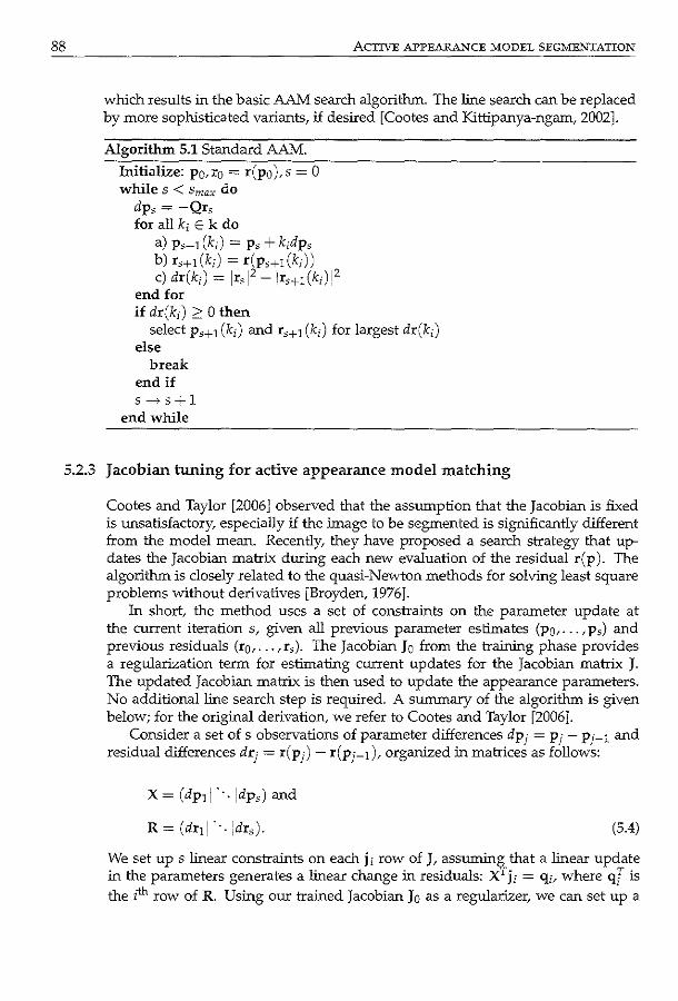
88 ACTIVE APPEARANCE MODEL SEGMENTATION

which results in the basic AAM search algorithm. The line search can be replaced by more sophisticated variants, if desired [Cootes and Kittipanya-ngam, 2002].

Algorithm 5.1 Standard AAM.

Initialize: po,ro = r(po),s = 0 while s < Smax do

dp, = -Qr, for all k; E k do

a) Ps+l (k;) = Ps + k;dp, b) rs+l(k;) = r(Ps+l(k;)) c) dr(k;) = Irs 12 - Jrs+l (k;) !

2

end for if dr(k;) 2 0 then

select Ps+l (k;) and r,+l (k;) for largest dr(k;) else

break end if s--:.s+l

end while

5.2.3 Jacobian tuning for active appearance model matching

Cootes and Taylor [2006] observed that the assumption that the Jacobian is fixed is unsatisfactory, especially if the image to be segmented is significantly different from the model mean. Recently, they have proposed a search strategy that up­dates the Jacobian matrix during each new evaluation of the residual r(p ). The algorithm is closely related to the quasi-Newton methods for solving least square problems without derivatives [Broyden, 1976].

In short, the method uses a set of constraints on the parameter update at the current iteration s, given all previous parameter estimates (po, ... , p,) and previous residuals (ro, ... , r,). The Jacobian Jo from the training phase provides a regularization term for estimating current updates for the Jacobian matrix J. The updated Jacobian matrix is then used to update the appearance parameters. No additional line search step is required. A summary of the algorithm is given below; for the original derivation, we refer to Cootes and Taylor [2006].

Consider a set of s observations of parameter differences dpj = Pi - Pi~ 1 and residual differences drj = r(pj)- r(pj~l), organized in matrices as follows:

X= (dp11·· .jdp,) and

R = (dr1! · ·. jdr,). (5.4)

We set up s linear constraints on each j; row of J, assumin~ that a linear update in the parameters generates a linear change in residuals: xrj; = q;, where qJ is the ith row of R. Using our trained Jacobian Jo as a regularizer, we can set up a

5.2 METHODS

quadratic function of the form f(ji) = a[XTji- q£1 2 + [j,- jo;[2, where a controls the strength of the regularization and j 0, is the zih row of Jo. Differentiating f with respect to j, and equating to zero, leads to an equation for computing a new estimate of J, given the initial estimate from the training set Jo and all previous parameter updates and residuals:

(5.5)

where I denotes the identity matrix. Eq. (5.5) can be rewritten into a more efficient version, which is then solved

iteratively. Let us define three matrices A = I + axxT , B = J6 + aXR T, and C = BTB. By substituting eq. (5.5) into eq. (5.3), it can be shown that the optimal parameter update is given by dp = Ay, if y is the solution to the linear equation Cy = -Brr. Instead of calculating A, B, and C using their definitions at every iteration, one can show that these matrices can be updated linearly at the current iteration s + 1 using their values at the previous iteration s:

As+l = As+ a5 dp,dp{

Bs+l = B, + a,dr,dp{ T T T 21 j2 T Cs+1 = Cs + a,B, dr5 dp5 + a5dp5 dr5 B, + a5 ,dr5 dp5 dp5 •

This leads to the Jacobian tuning algorithm for AAM matching:

Algorithm 5.2 Jacobian-Tuning AAM.

Initialize: p0, r0 = r(p0), s = 0, A0 =I, B0 = J0, C0 = BJ"B0 while [dp5 [

2 < e and s < Srnax do 1) Solve C,y = - B{ r5 for y 2) dp, = A,y 3) Ps-'-1 = Ps + dp, 4) r,~ 1 = r(Ps+l) 5) drs = rs+l - r, 6) z = B{dr5

7) As+l = As+ a5dp5dp{ 8) Bs+l = Bs + a5dr5dp{ 9) Cs+1 = C, +a,zdp{ +a,dp5zT +a~[dr,j2dp5dp{ if [rs+1[ 2 > [r,[ 2 then

Ps-71 = Ps, rs+l = rs end if 11) s ___, s+1

end while

(5.6)

The resulting algorithm has only a series of simple linear operations, and can therefore be added straightforwardly to any existing AAM implementation. Note that the matrices A, B, and C are updated every iteration, regardless of the parameter update. It is usually possible to solve the linear equation in step 1 using Cholesky decomposition, as C, is symmetric and (usually) positive definite. As in

89

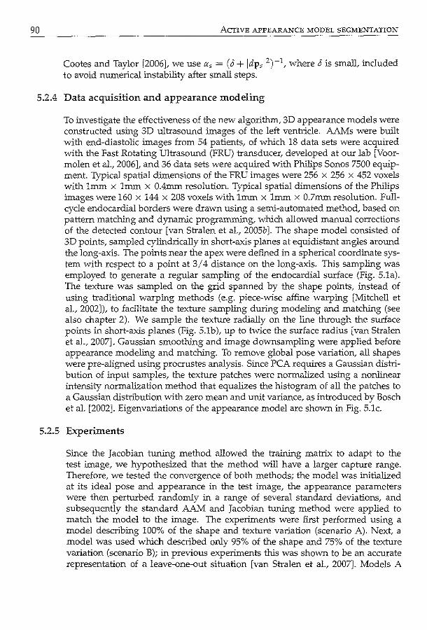
90 ACTIVE APPEARANCE MODEL SEGMENTATION

Cootes and Taylor [2006], we use C<s = (J + ldp,l 2)-1, where J is small, included to avoid numerical instability after small steps.

5.2.4 Data acquisition and appearance modeling

To investigate the effectiveness of the new algorithm, 3D appearance models were constructed using 3D ultrasound images of the left ventricle. AAMs were built with end-diastolic images from 54 patients, of which 18 data sets were acquired with the Fast Rotating Ultrasound (FRU) transducer, developed at our lab [Voor­molen et a!., 2006], and 36 data sets were acquired with Philips Sonos 7500 equip­ment. Typical spatial dimensions of the FRU images were 256 x 256 x 452 voxels with 1mm x 1mm x 0.4mm resolution. Typical spatial dimensions of the Philips images were 160 x 144 x 208 voxels with 1mm x 1mm x 0.7mm resolution. Full­cycle endocardial borders were drawn using a semi-automated method, based on pattern matching and dynamic progranuning, which allowed manual corrections of the detected contour [van Stralen et al., 2005b]. The shape model consisted of 3D points, sampled cylindrically in short-axis planes at equidistant angles around the long-axis. The points near the apex were defined in a spherical coordinate sys­tem with respect to a point at 3 I 4 distance on the long-axis. This sampling was employed to generate a regular sampling of the endocardial surface (Fig. 5.1a). The texture was sampled on the grid spanned by the shape points, instead of using traditional warping methods (e.g. piece-wise affine warping [Mitchell et al., 2002]), to facilitate the texture sampling during modeling and matching (see also chapter 2). We sample the texture radially on the line through the surface points in short-axis planes (Fig. 5.1b), up to twice the surface radius [van Stralen eta!., 2007]. Gaussian smoothing and image downsampling were applied before appearance modeling and matching. To remove global pose variation, all shapes were pre-aligned using procrustes analysis. Since PCA requires a Gaussian distri­bution of input samples, the texture patches were normalized using a nonlinear intensity normalization method that equalizes the histogram of all the patches to a Gaussian distribution with zero mean and unit variance, as introduced by Bosch eta!. [2002]. Eigenvariations of the appearance model are shown in Fig. 5.1c.

5.2.5 Experiments

Since the Jacobian tuning method allowed the training matrix to adapt to the test image, we hypothesized that the method will have a larger capture range. Therefore, we tested the convergence of both methods; the model was initialized at its ideal pose and appearance in the test image, the appearance parameters were then perturbed randomly in a range of several standard deviations, and subsequently the standard AAJv! and Jacobian tuning method were applied to match the model to the image. The experiments were first performed using a model describing 100% of the shape and texture variation (scenario A). Next, a model was used which described only 95% of the shape and 75% of the texture variation (scenario B); in previous experiments this was shown to be an accurate representation of a leave-one-out situation [van Stralen et a!., 2007]. Models A

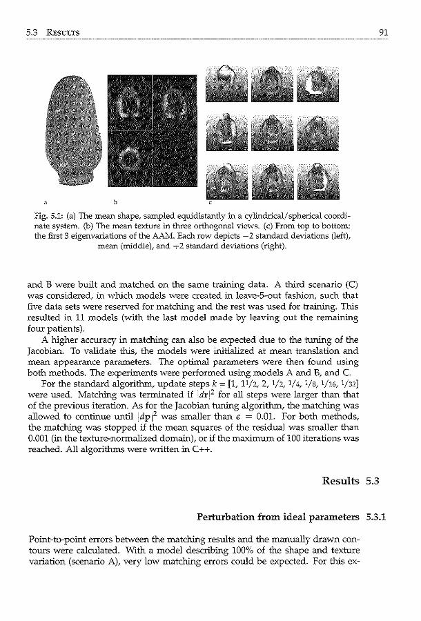
5.3 RESULTS

a b

fig. 5.1: (a) The mean shape, sampled equidistantly in a cylindrical/ spherical coordi­nate system. (b) The mean texture in three orthogonal views. (c) From top to bottom: the first 3 eigenvariations of the AAM. Each row depicts -2 standard deviations (left),

mean (middle), and -,-2 standard deviations (right).

and B were built and matched on the same training data. A third scenario (C) was considered, in which models were created in leave-S-out fashion, such that five data sets were reserved for matching and the rest was used for training. This resulted in 11 models (with the last model made by leaving out the remaining four patients).

A higher accuracy in matching can also be expected due to the tuning of the Jacobian. To validate this, the models were initialized at mean translation and mean appearance parameters. The optimal parameters were then found using both methods. The experiments were performed using models A and B, and C.

For the standard algorithm, update steps k = [1, 11/2, 2, 1/2, 1/4, 1/s, 1/16, 1/32] were used. Matching was terminated if jdr[2 for all steps were larger than that of the previous iteration. As for the Jacobian tuning algorithm, the matching was allowed to continue until jdpj2 was smaller than € = 0.01. For both methods, the matching was stopped if the mean squares of the residual was smaller than 0.001 (in the texture-normalized domain), or if the maximum of 100 iterations was reached. All algorithms were written in C++.

Results 5.3

91

Perturbation from ideal parameters 5.3.1

Point-to-point errors between the matching results and the manually drawn con­tours were calculated. With a model describing 100% of the shape and texture variation (scenario A), very low matching errors could be expected. For this ex-

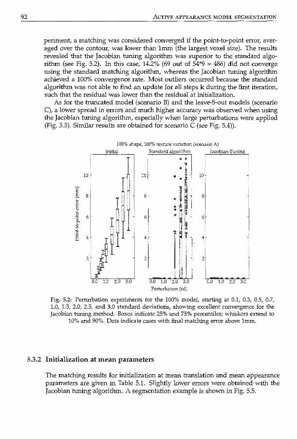
92 ACTIVE APPEARANCE MODEL SEGMENTATION

periment, a matching was considered converged if the point-to-point error, aver­aged over the contour, was lower than 1mm (the largest voxel size). The results revealed that the Jacobian tuning algorithm was superior to the standard algo­rithm (see Fig. 5.2). In this case, 14.2% (69 out of 54*9 = 486) did not converge using the standard matching algorithm, whereas the Jacobian tuning algorithm achieved a 100% convergence rate. Most outliers occurred because the standard algorithm was not able to find an update for all steps k during the first iteration, such that the residual was lower than the residual at initialization.

As for the truncated model (scenario B) and the leave-S-out models (scenario C), a lower spread in errors and much higher accuracy was observed when using the Jacobian tuning algorithm, especially when large perturbations were applied (Fig. 5.3). Similar results are obtained for scenario C (see Fig. 5.4)).

10 .

E' .s 8

6

4

100% shape, 100% texture variation (scenario A)

Initial I Standa'd algo:u:.m I _Jacobian-Tuninp_,

10· • ·1·' 10·

8

6

4.

2

0.0 1.0 2.0 3.0

H, s

;~; o H F ~!I n,. 6

- ~ ~· 4·

2LJ 0.0 1.0 2.0 3.0

Perturbation (sd)

0.0 1.0 2.0 3.0

fig. 5.2: Perturbation experiments for the 100% model, starting at 0.1, 0.3, 0.5, 0.7, 1.0, 1.5, 2.0, 2.5, and 3.0 standard deviations, showing excellent convergence for the Jacobian tuning method. Boxes indicate 25% and 75% percentiles; whiskers extend to

10% and 90%. Dots indicate cases with final matching error above lm.m.

5.3.2 Initialization at mean parameters

The matching results for initialization at mean translation and mean appearance parameters are given m Table 5.1. Slightly lower errors were obtained with the Jacobian tuning algorithm. A segmentation example is shown in Fig. 5.5.

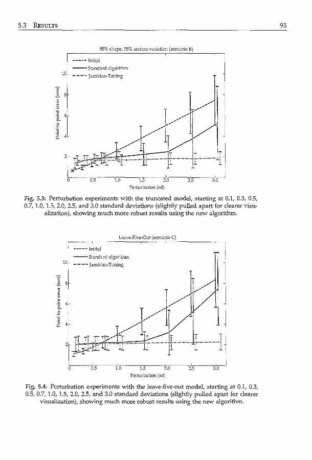
5.3 RESULTS

95% sl10.pe, 75% texture variation (scemrio B)

----- Initial

--St.mdard algorithm

lO, -·-·-·- Jacobi.m-Tuning

1

J ~~:p:r ~::::lr.:=:=u I J:'_. ...

0 0.5 1.0 1.5 2.0 2.5 3.0

Perturbation (sd)

Fig. 5.3: Perturbation experiments with the truncated model, starting at 0.1, 0.3, 0.5,. 0.7, 1.0, 1.5, 2.0, 2.5, and 3.0 standard deviations (slightly pulled apart for clearer visu­

alization), showiD.g much more robust results using the new algorithm.

Leave-Five-Out (scenario C)

0 0.5 1.0 1.5 2.0 2.5 3.0

Pcrlurb.J.tion (sd)

Fig. 5.4: Perturbation experiments with the leave-five-out model, starting at 0.1, 0.3, 0.5, 0.7, 1.0, 1.5, 2.0, 2.5, and 3.0 standard deviations (slightly pulled apart for clearer

visualization), showing much more robust results using the new algorithm.

93

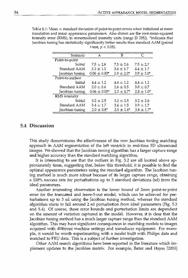
94

5.4

ACTIVE APPEARANCE MODEL SEGMENTATION

Table 5.1: Mean ± standard deviation of point-to-point errors when initialized at mean translation and mean appearance parameters. Also shown are the root-mean-squared intensity error (RMS), in unnormalized intensity units (range [0 255]). *indicates that Jacobian tuning has statistically significantly better results than standard AAM (paired

!-test, p < 0.05).

Scenario A B c PoiDt-to-point

Initial 7.5 = 2.6 7.5 ± 2.6 7.5 ± 2.7 Standard AAM 2.3 ± 1.1 3.6 ± 1.7 4.4 ± 1.7 Jacobian tuning 0.06 ± 0.03* 2.9 ± 2.0* 3.9 ± 2.0*

Point-to-surface Initial 4.4 ± 1.2 4.4 ± 1.2 4.4 ± 1.2

Standard AAM 2.0 ± 0.6 2.6 = 0.5 3.0 = 0.7 Jacobian tuning 0.06 ± 0.03* 2.2 ± 0.7* 2.8 ± 1.0*

RMS intensity Initial 5.2 ± 2.5 5.2 ± 2.5 5.2 ± 2.6

Standard AAM 3.4 ± 1.7 3.6 ± 1.5 3.9 ± 1.7 Jacobian tuning 2.0 ± 0.8* 3.5 ± 1.6* 3.8 ± 1.7*

Discussion

This study demonstrates the effectiveness of the new Jacobian tuning matching approach in AAM segmentation of the left ventricle in real-time 3D ultrasound images. We showed that the Jacobian tuning algorithm has a larger capture range and higher accuracy than the standard matching algorithm.

It is interesting to see that the outliers in Fig. 5.2 are all located above ap­proximately 4mm, suggesting that, below this threshold, it is possible to find the optimal appearance parameters using the standard algorithm. The Jacobian tun­ing method is much more robust because of its larger capture range, obtaining a 100% success rate for perturbations up to 3 standard deviations (sd) from the ideal parameters.

Another interesting observation is the lower bound of 2mm point-to-point error for the truncated and leave-S-out model, which can be achieved for per­turbations up to 3 sd using the Jacobian tuning method, whereas the standard algorithm starts to fail around 2 sd perturbation from ideal parameters (Fig. 5.3 and 5.4). Of course, these error bounds and perturbation limits are dependent on the amount of variation captured in the model. However, it is clear that the Jacobian tuning method has a much larger capture range than the standard AAM algorithm. This may have significant consequences in matching models to images acquired with different machine settings and transducer equipment. For exam­ple, it would be worth experimenting with a model built with Philips data and matched to FRU data. This is a subject of further investigation.

Other AAM search algorithms have been reported in the literature which im­plement updates to the Jacobian matrix. For example, Batur and Hayes [2005]

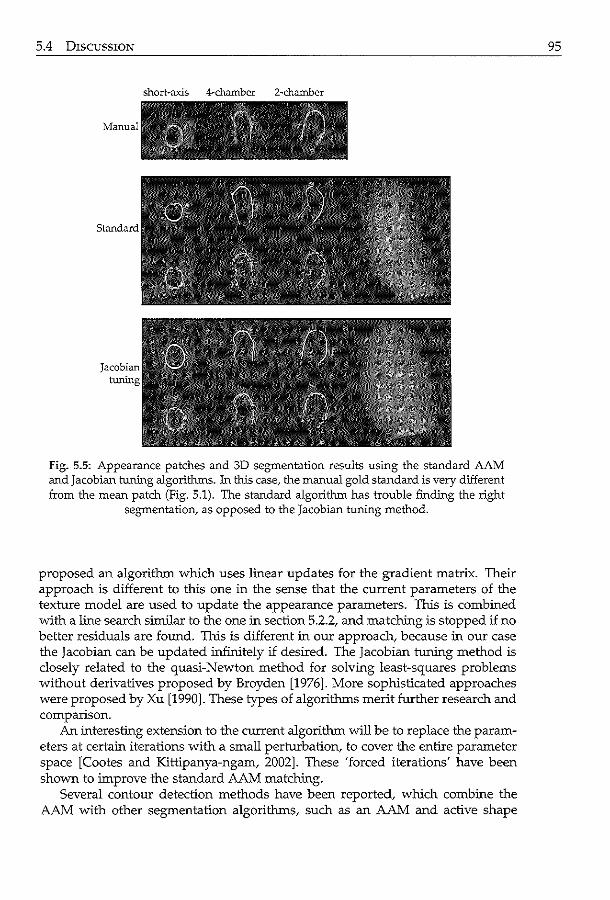
5.4 DISCUSSION

Jacobian tuning

short-axis 4-chamber 2-chamber

Fig. 5.5: Appearance patches and 3D segmentation results using the standard AAM and jacobian tuning algorithms. In this case, the manual gold standard is very different from the mean patch (Fig. 5.1). The standard algorithm has trouble finding the right

segmentation, as opposed to the Jacobian tuning method.

proposed an algorithm which uses linear updates for the gradient matrix. Their approach is different to this one in the sense that the current parameters of the texture model are used to update the appearance parameters. This is combined with a line search similar to the one in section 5.2.2, and matching is stopped if no better residuals are found. This is different in our approach, because in our case the Jacobian can be updated infinitely if desired. The Jacobian tuning method is closely related to the quasi-Newton method for solving least-squares problems without derivatives proposed by Broyden [1976]. More sophisticated approaches were proposed by Xu [1990]. These types of algorithms merit further research and comparison.

An interesting extension to the current algorithm will be to replace the param­eters at certain iterations with a small perturbation, to cover the entire parameter space [Cootes and Kittipanya-ngam, 2002]. These 'forced iterations' have been shown to improve the standard AAM matching.

Several contour detection methods have been reported, which combine the AAM with other segmentation algorithms, such as an AAM and active shape

95

96 ACTIVE APPEARANCE MODEL SEGMENTATION

model hybrid [Mitchell et al., 2001], AAM and pixel classification hybrid [van Ginneken et al., 2006], and information fusion approaches [Comaniciu et al., 2004]. Also, there have been a number of reports on multiview [Bosch et al., 2002; Uzfuncii et al., 2005] or multifeature AAMs [Scott et al., 2003]. All could benefit from the Jacobian tuning method. Since the AAM is becoming a widely used segmentation technique in medical image processing, the method appears to be particularly relevant for this scientific community. The large improvements that it has to offer may cause the Jacobian tuning method to be set as the standard matching approach some day.

5.5 Conclusions

The new Jacobian tuning algorithm for AAM matching produces quantitatively better segmentations of the left ventricle in ultrasound images. This study demon­strates the effectiveness of an adaptive training matrix during model matching. Given the large variability in ultrasound image appearance, the Jacobian tuning algorithm has great potential in improving the standard AAM segmentation.

Motion-guided optical flow tracking in 3D echocardiograms To obtain quantitative and objective functional parameters from 3D echocardiograms, the use of automated segmentation methods is becoming increasingly important. In this chapter, we propose an optical-flow based tracking method to propagate 3D en­docardial contours throughout the cardiac sequence. To take full advantage of the time-continuous nature of the cardiac motion, a pre-trained statistical motion model was used to guide the optical-flow solution. The algorithm. was tested on 53 non­contrast echocardiographic sequences. For high quality images.~ the combination of the proposed motion-guided method and a purely data-driven local tracking method provided optimal surface estimation with low error (point-to-surface: 1.4 ± 0.4mrn, absolute volume 5.6 ± 4.Sml). For low quality images, the motion-guided algorithm was superior. Application to 27 contrast-enhanced images also revealed encouraging results. This demonstrates the method's potential in automated tracking in a variety of clinical 3D echocardiographic protocols.

Dcrivcd from: Motion·Guided Optical Flow fot Tt.acking in 3D Echocardiograms K Y.E. Leung, M.G. Danilouchkine, M. wn StrJ.lcn, 1\'. de Jong.. A.F.W. v.:m der Steen, .:md J.G. Bosch Proc SPIE Mcd Im.:!g 2009; i259; 7>...590W.

98 OPTICAL FLOW TRACKING

6.1 Introduction

Echocardiography is a commonly used, safe, and noninvasive technique that al­lows the assessment of left ventricular (LV) function. Real-time 3D echocardio­graphy has gained much interest in recent years. The advantage of acquiring the whole left ventricle in a short period of time, plus recent improvements in spatial and temporal resolution, have made this method a viable alternative to traditional 2D echocardiography. Due to the large amount of data acquired, there is an increasing demand for automated methods to analyze LV functional param­eters, such as LV volume, accurately and objectively. Therefore, segmentation in 3D and 4D (3D+time) echocardiograrns has gained considerable attention recently [Noble and Boukerroui, 2006]. Common automated methods include deformable models [Gerard et al., 2002; Montagnat et al., 2003; Nillesen et al., 2007; Walimbe et al., 2006], level sets [Angelini et al., 2005; Corsi et al., 2002], active appearance and active shape model techniques [Hansegard et al., 2007b; van Stralen et al., 2007], state estimation [Orderud et al., 2007b], and clustering/ classification [Pa­pademetris et al., 2001; Sanchez-Ortiz et al., 2002].

To approach 4D segmentation efficiently, one can choose to explicitly distin­guish between spatial and temporal differences in anatomical shape. Similar types of distinctions between variations were previously exploited in Costen et al. [2002]; Lorenzo-Valdes et al. [2004]; Perperidis et al. [2005] for segmentation and modeling. In the medical imaging context, spatial variation is related to anatomi­cal diversity across different patients, which can be used as priors in segmenting one 3D image. Temporal variation captures the variability in an organ's shape due to physiological activity. This knowledge can help propagate the segmenta­tion throughout the image sequence. The present chapter focuses on the latter aspect, which is tracking related.

It is well known that good ultrasound segmentation needs to make use of ali task-specific constraints, as recently stressed in Noble and Boukerroui [2006]. Therefore, it is crucial for tracking in echocardiograrns to incorporate temporal knowledge, in order to obtain consistent contours throughout the cardiac cy­cle. Hence, we propose to incorporate anatomical motion models into the track­ing scheme, to produce reliable segmentations that are likely to occur in in vivo echocardiograrns.

6.1.1 Previous work

Many ideas for tracking objects in images have been developed within the hu­man vision research community [Yilmaz et al., 2006]. Recently, tracking in ultra­sound cardiac images, especially in 3D, has become a popular field of research [Angelini and Gerard, 2006]. Tracking methods can be based on deformation of surfaces [Yan et al., 2007] or on tracking image intensities. Most commonly used intensity-based tracking techniques include nomigid registration [Elen et al., 2008; Ledesma-Carbayo et al., 2005; Myronenko et al., 2007], Bayesian techniques [Pa­pademetris et.al., 2001], template/block matching [Duan et al., 2008; Helle-Valle et

6.1 INTRODUCTION

al., 2005; Kawagishi, 2008; Linguraru et al., 2008; Yeung et al., 1998b]_ and optical flow [Siihling et al., 2005; Veronesi et al., 2006]. If the images differ considerably, nonrigid registration may prove more accurate than the other methods. However, if these differences are small, the latter two techniques may suffice.

In this work, we chose to explore a framework based on differential optical flow tracking [Hom and Schunck, 1981; Lucas and Kanade, 1981]. The main ad­vantages of our method lie in its flexibility to incorporate motion information, its accuracy in tracking, and a lower computational demand compared with nonrigid registration. Unlike most applications in ultrasound imaging (e.g. Danilouchkine et al. [2008]), we intend to use the optical flow method to track the endocardial border in the images, and not individual speckle patterns. The tracking is per­formed in time-gain-compensated envelope data, and not the raw radio-frequency data. This is important to note, because current 3D ultrasound images are often acquired at a lower frame rate with respect to two-dimensional images. Therefore, the speckle pattern varies greatly from frame to frame.

Optical flow based methods have previously been applied for motion analysis, modeling, and segmentation in medical imaging. Most methods use the Hom­Schunck solution [Horn and Schunck, 1981], which applies a global smoothness constraint on the motion field, or the Lucas-Kanade solution [Lucas and Kanade, 198lt which assumes local motion consistency. For magnetic resonance (MR), op­tical flow based methods have mainly been applied to estimate motion in cardiac images [Dougherty et al., 1999; Florack et al., 2007] and brain images [Hata et al., 2000; Tosun and Prince, 2005]. There are also reports on optical flow for com­puted tomography (CT) images [Gorce et al., 1997; Kalmoun et al., 2007; Song and Leahy, 199lt SPECT images [Laliberte eta!., 2004; Noumeir eta!., 1996L and PET images [Lin and Lin, 2004].

As for ultrasound cardiac imaging, Mailloux et al. [1987] applied the Horn­Schunck solution to analyze 2D echocardiograms. Baraldi et al. [1996] compared three algorithms on synthesized ultrasound images and concluded that the Horn­Schunck and Lucas-Kanade approaches generated more favorable results than the Nagel method [Nagel. 1987]. Left ventricular wall motion was analyzed us­ing a basic implementation of the Lucas-Kanade method by Chunke et al. [1996]. Mikic et al. [1998] first used optical flow for propagating contours throughout echocardiograms. The optical flow was used to initialize the contour in the sub­sequent frame, after which the actual contour detection was performed by active contours. More recently Siihling et al. [2005] developed a combination of optical flow and b-splines to segment 2D echocardiographic sequences. An application for 3D echocardiography was described by Veronesi et al. [2006]. In their paper, the Lucas-Kanade approach was used together with a block matching procedure to detect the long-axis of the left ventricle. The novel aspect of the current method is the incorporation of a trained statistical motion model, to generate consistent 4D contours throughout the cardiac cycle.

Several methods for incorporating shape models with segmentation have been reported in the literature. An interesting approach was described by Malassiotis and Strintzis [19991 who constrained an active contour based segmentation by applying principal component analysis (PCA) over the contour sequence at hand.

99

100 OPTICAL FLOW TRACKING

This is different from our approach, because the model here is trained with con­tours of many sequences. Comaniciu et al. [2004] proposed projecting optical flow estimates back to the shape model space to generate a more robust segmen­tation. They used the mean shift method to combine multiple optical flow esti­mates. Hansegiird et a!. [2007b] proposed to estimate shape model parameters in a Kalman filtering approach, using estimates in the previous time-frames to gen­erate new parameters for the current frame. Their algorithm was real-time, with the trade-off that it was less accurate. The approach taken in the current chap­ter is different, because motion parameters were derived from shapes throughout the cardiac cycle, resulting in a time-continuous motion model. Recently, Per­peridis et al. [2007] suggested a segmentation method using registration with a shape model. This model was decoupled into two parts: interpatient statistics (spatial variations) and intrapatient statistics (temporal variations). The model parameters were numerically optimized in nonrigid-registration fashion, using a gradient-descent approach and a gradient-based similarity measure. Our work is different because we make use of an optical flow formulation to solve the reg­istration problem. It can be considered as a light-weight solution as it allows a close form solution.

6.1.2 Study outline

In this chapter, we propose to combine optical flow tracking with learned patterns of motion. This method is different from the technique proposed by Comaniciu et al. [2004], who combined optical flow estimates and active appearance mod­els using information fusion. Instead, our approach most resembles the method proposed by Yacoob and Davis [2000] for estimating human motion in 2D video sequences. The motion model is derived from manually delineated 4D contours, which should result in a realistic modeling of myocardial wall motion. To en­hance the local tracking accuracy, the motion-guided approach is combined with purely data-driven optical flow tracking. The algorithm is tested on 53 noncon­trast 4D echocardiograms, recorded using different acquisition equipment. As an extension, the method is also applied to 27 contrast-enhanced echocardiograms.

6.2 Methods

The general idea of the proposed motion-guided segmentation method is to com­bine optical flow tracking with learned patterns of motion, derived from manually drawn 4D contours of the LV endocardial borders. The motion model is then ex­plicitly embedded in the optical flow equation and motion-model parameters are resolved using spatial and temporal image gradients. To enhance the tracking performance in good quality images, the method is combined with a basic local Lucas-Kanade tracker.

6.2 METHODS 101

Optical flow basics 6.2.1

Optical flow tracking aims at finding the apparent motion ('flow') of objects in an image sequence. The method relies on the assumption that the image intensities of the object during movement are constant: I(x, t) = I(x + dx, t + dt), where I is the intensity at spatial coordinates x and time t. By applying first-order Taylor expansion, the well-known optical flow equation is obtained, which describes the relationship between the motion field (v), the spatial (vI = ( ¥x, g~, ~) =

(I, Iy, I0 )) and temporal gradient (I,= Ml in image intensity:

vi(x, t) · v(x, t) + I1(x, t) = 0. (6.1)

v consists of the velocity components of the motion field; for 3D images, v = ( Vx(a), vy( a), v0 ( a)). Each velocity component can be described with k parameters a, to denote different types of velocity models (e.g. translation-only, similarity, or affine).

To solve eq. (6.1) for v, more assumptions are required, because this one equa­tion contains k unknowns. The commonly-used Lucas-Kanade approach assumes that the velocity is constant in a small region around x, in which N gradients are sampled. In this study, we use a symmetric kernel of size nw x nw x nw. The velocity vector can then be resolved with least-squares. A sum-of-squares error term is set up as follows [Lucas and Kanade, 1981]:

N E = E (w(x(n)))2 [I,(x(n)) + vi(x(n)). v] 2

' (6.2) n=l

where w represents a local weight. For a translation-only description of v, this can be solved by differentiating eq. ( 6.2) with respect to each translation component v = ( Vx, Vy, v2 ), and equating the result to zero. This leads to the following system of equations (note that w, Iu, Iv and It depend on n ):

Rv = e, with N

Ruv = L, w2 Iulv, and n=l

N

eu=-Lzif-Itiu for u,v=x,y,z. n=l

(6.3)

Shape-based motion modeling 6.2.2

In this work, the optical flow equation is regularized with a motion model, trained using contours of in vivo data sets. These contours are represented by the 3D co­ordinates of points which are evenly distributed on the endocardial surface. We chose to model the cardiac motion on a frame-to-frame basis, because the in­tensity difference between two consecutive images is smaller than the difference between a reference frame (e.g. in end-diastole) and all subsequent frames. This is

102 OPTICAL FLOW TRACKING

important because the optical flow equation assumes brightness invariance, and optical flow has proven to have a suboptimal accuracy in tracking large displace­ments [Danilouchkine et al., 2008]. For the modeling itself, principal component analysis (PCA) is used, which generates a compact representation of the motion parameters. This is much more efficient and robust than e.g. direct modeling of the motion parameters, because PCA reduces the dimensionality of the input data, disregarding noisy components. Our approach is different from traditional statistical shape models [Cootes et al., 2001], which describe the statistical varia­tion of the shape using the actual contour points themselves, because we model the motion using affine parameters which are extracted from the training con­tours.

Furthermore, for a time-continuous result, we choose to model and resolve the motion vectors by considering the whole cardiac cycle simultaneously. The goal of the proposed optical flow method is to provide a globally consistent tracking result, for estimating global parameters such as left ventricular volume. There­fore, as a good approximation, one affine transform may be sufficient to explain a frame-to-frame difference. Although this may seem a rather tight restriction, we anticipate that this representation will have a small error, because of limited dif­ferences between two consecutive frames. Also, as for any modeling technique, the amount of input data strongly influences the level of model generalization. In the 4D case, the modeling of local variation may require a great many patient data sets, which is often unavailable in practice. Therefore, we choose to model only the global motion, and will further refine the segmentation using a more local tracking algorithm.

The motion is modeled as affine transforms of the contour from one frame to the next, where the changes throughout the cardiac cycle are characterized by translation, rotation, shear, and scaling. The steps in motion modeling are visual­ized in Fig. 6.1 and are described below. Affine parameters in 3D are modeled as follows:

v= (6.4)

Phase normalization

Since PCA requires each input to have an equal number of affine parameters, all contours must be normalized to a common division of the cardiac phase. As the left ventricle contracts in systole and expands in diastole, we propose to match the end-diastolic (ED) and end-systolic (ES) time-points in all contour sequences. For each phase, the 3D contour is represented by points, distributed on the endocar­dial surface. All contour sequences are then linearly interpolated between frames to generate sequences in the normalized phase division, so that each sequence contains F cardiac phases.

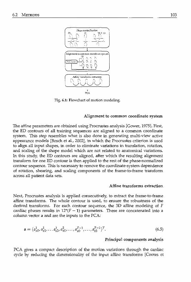
6.2 METHODS

Ph.l~ normilli7.<ttion ED-1 CD

", : '·

Alignment to common coordinJt<;> ~t<:m

~r.J? ~. ~. :', .

l'rncru·•lt'' "<;I ~ ~ i'J )\

L c.,?~'i?

Affine tr.msfonn~ o;'Xtrilction

·:\ (\. 0_ '' .:-",

·v-v\ ... /V l

PCA

Fig. 6.1: Flowchart of motion modeling.

Alignment to common coordinate system

The affine parameters are obtained using Procrustes analysis [Gower, 1975]. First, the ED contours of all training sequences are aligned to a common coordinate system. This step resembles what is also done in generating multi-view active appearance models [Bosch eta!., 2002], in which the Procrustes criterion is used to align all input shapes, in order to eliminate variations in translation, rotation, and scaling of the shape model which are not related to anatomical variations. 1n this study, the ED contours are aligned, after which the resulting alignment transform for one ED contour is then applied to the rest of the phase-normalized contour sequence. This is necessary to remove the coordinate-system dependence of rotation, shearing, and scaling components of the frame-to-frame transform across all patient data sets.

Affine transforms extraction

Next, Procrustes analysis is applied consecutively, to extract the frame-to-frame affine transforms. The whole contour is used, to ensure the robustness of the derived transforms. For each contour sequence, the 3D affine modeling of F cardiac phases results in 12*(F- 1) parameters. These are concatenated into a column vector a and are the inputs to the PCA:

(6.5)

Principal components analysis

PCA gives a compact description of the motion variations through the cardiac cycle by reducing the dimensionality of the input affine transforms [Cootes et

103

104 OPTICAL FLOW TRACKING

a!., 2001]. This allows us to approximate a set of affine warps a throughout the cardiac cycle using the mean transform a, the PCA eigenvectors <I> and the PCA parameters c:

a"" a+ <I>c. (6.6)

Since the eigenvectors are sorted :in order of variance, modes with low variance can be removed easily by truncating c and <I>. The remaining k modes will then encompass only a proportion g of the total variation G:

k I;?.; 2: gG, i=l

p

with G = L;J.1,

i=l (6.7)

where p is the total number of modes and A; denotes the i1h eigenvalue [Mitchell et a!., 2002]. With formula (6.6), the frame-to-frame affine transform throughout the cardiac cycle is described by k parameters c, which are to be solved with optical flow. k thus depends on the choice of g. For this study, g = 95% is used, corresponding with k = 24 parameters for a model built with 35 noncontrast contours, and k = 18 parameters for a model built with 27 contrast contours.

6.2.3 Motion-guided segmentation

One of the main ideas of this work is to combine the learned motion model with the optical flow equation directly. This results in an efficient and elegant solution to the optical flow equation, guided by the typical motion patterns encountered in a set of training examples. Each affine component ai (formula (6.4)) of a certain cardiac phase f can be described with the corresponding row of <I> and the correct components of a and c:

(6.8)

This is substituted in each affine component in formula (6.4) and this in turn is substituted in eq. (6.1). This leads to the modified optical flow equation:

E(x,t) =I,+ Ixiix + Iyiiy + Iziiz + (Ix<l>x + Iy<l>y + Iz<I>z) C = 0 (6.9)

h - -! + -! + -! + -f w ere ad xadO yadl zad2 ad3 f d f f ~f f or =x,y,z. and <I> d = x<I> do + y<I> dl + z<i>'d2 + <I> d3

The objective is to find c, given the spatial gradients Ix, Iy, Iz and temporal gra­dient I,. A solution is to constrain the equation by assuming that the parameters c are identical in all regions and all cardiac phases, similar to the Lucas-Kanade approach (formula (6.2)). We can then set up a sum-of-squares error term Etotaz:

N F-1

€total = I:;I:;[E(xJ)f =I; I; [E(n,t)f, (6.10) x f n=l f=l

6.2 METHODS

by gathering the image gradients from N voxel positions per image. These are gathered from regions of nw x nw x nw around each contour point (like in eq. (6.2)). By differentiating <total to each element in c and setting this to zero, a system of linear equations is obtained, similar to eq. (6.3):

Rc = e, (6.11)

where R is a k-by-k symmetrical matrix, and c and e are k-by-1 vectors:

N F-1

Ruv = L L w2 ( Ixi/J~ + Iyi/J~ + Izi/J~) ( Ixi/J~ + Iyi/J~ + Izi/J~)

n=1f=1

N F-1

eu = - L L w2 (It + Ixiix + Iyiiy + Iziiz) ( Ixi/J~ + Iyi/J~ + Izi/J~) n=1f=1

(6.12)

where <P'd is the uth element of~' the row in the eigenvector matrix correspond­ing with phase f (note that all terrns depend on n). Since R is symmetric and usually positive definite, eq. (6.11) can be solved e.g. with Cholesky decomposi­tion.

105

Algorithm scheme 6.2.4

In practice, the algorithm needs a 3D contour of the end-diastolic frame as a start­ing point for 4D segmentation in a testing image. In this study, the manually delineated ED contour is taken. The spatial derivatives are calculated by convolu­tion with a Gaussian derivative filter (for !T see Table 6.1). Our implementation of optical flow conforms to the principle of reciprocity in image disparity [Birchfield and Tomasi, 1998]. In other words, if a given point x in the first image moves in the direction d, then the point x + d in the second image travels the same distance in the opposite direction. Based on this fact, one may obtain the optical flow equation, which ties together the components of the vector velocity field with the spatial derivatives computed over the average of two consecutive frames and the temporal derivatives calculated as their difference [Birchfield, 1999]. Tempo­ral derivatives are computed by taking the finite difference between two image frames. The weight w in formula (6.12) was 1 if the voxel was inside the trans­ducer's imaging sector, and 0 otherwise, to prevent the influence of the image sector borders on tracking.

To achieve temporal aligrunent, we chose to adapt the normalized phase di­vision to match the phase division of the test image, by generating new motion models for each test image separately. To achieve spatial aligrunent, the ED con­tour of the test image was first transformed to the common coordinate system. This was achieved by aligning the ED contour of the test image and the average of the training contours using Procrustes analysis. The spatial transform is used in the gathering of the terms in formula (6.12) and for applying the ED contour to the test image (step (D) of alg. 6.1). The pseudo-code in alg. 6.1 illustrates the steps for resolving the tracking parameters.

106 OPTICAL FLOW TRACKrNG

Algorithm 6.1 Motion-guided tracking scheme.

(A) for each image pair f (1) calculate spatial and temporal derivatives (2) sample gradients on N positions around current contour (3) populate formula (6.12) for frame pair f

(B) Solve eq. (6.11) for c (C) Convert c into affine parameters a (formula (6.6)) (D) Apply a to ED contour frame-by-frame

6.2.5 Combined tracking

Since the frame-to-frame affine transform is derived from the whole 3D contour, the model will contain global patterns of motion. This is useful in image regions without salient structures.' e.g. :in regions with shadow-artifact or with low signal­to-noise ratio. However, due to the global nature of the motion-guided method, slightly less accurate results may be obtained locally, in particular if local patholo­gies are present. This will be especially noticeable at sites with clear structures. ln an initial feasibility study, we found that the non-motion-guided Lucas-Kanade approach (denoted as basic tracking in the following; formula (6.3)) was able to track areas with salient structures very accurately, but performed poorly in other regions. Therefore, we hypothesize that the combination of the proposed motion­guided method and this basic Lucas-Kanade tracking would enhance the tracking performance. Since the basic tracking was sensitive to noise, we also anticipate that this combination is only useful if the images are of sufficient quality.

The combined result is determined by transforming the ED contour frame-by­frame, using weighed results of both methods. Each point on the contour at frame s - 1 is transformed to coordinates Xcombined' determined by weighing the results of the basic tracking (xB) and the motion-guided method (xMc) as follows:

x;ombined = f3x!J + (1 - f3)x';;rc- (6.13)

f3 is a weight, which is determined by the tracking accuracy (f3 A) and the presence of salient structures (f3s) around the point:

f3 = (f3A + f3s)/2. (6.14)

The tracking accuracy is defined as the sum-of-squares difference in intensity between two frames, in an area surrounding the point, as this was the tracking error term (formula (6.2), 6.10). f3 A is 1 if this difference is lower for Lucas-Kanade approach than for the motion-guided method, and 0 otherwise.

To detect areas with salient structures, the gradient norm I \7 I I of the 3D+ T sequence was used. A quadratic function is used to convert the gradient norm around the point to a weight. A quadratic function is used because of the lower slope around [vi[min' so that the motion-guided method contributes more in areas with possible noise.

f3s = ( !VI[- jvifmm )2

lvi[max -[vi[mm (6.15)

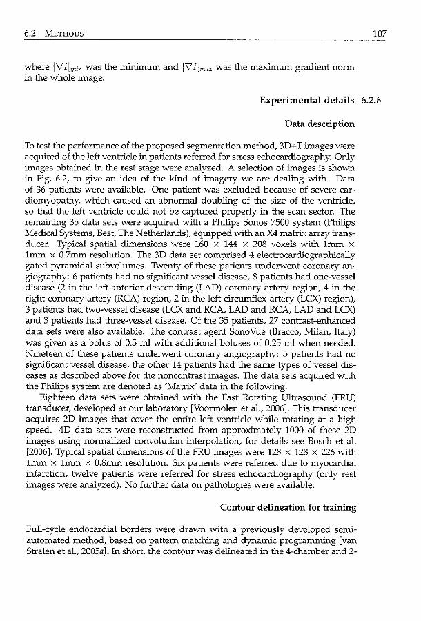
6.2 METHODS

where IVIImin was the minimum and IVIImax was the maximum gradient norm in the whole image.

107

Experimental details 6.2.6

Data description

To test the performance of the proposed segmentation method, 3D+ T images were acquired of the left ventricle in patients referred for stress echocardiography. Only images obtained in the rest stage were analyzed. A selection of images is shown in Fig. 6.2, to give an idea of the kind of imagery we are dealing with. Data of 36 patients were available. One patient was excluded because of severe car­diomyopathy, which caused an abnormal doubling of the size of the ventricle, so that the left ventricle could not be captured properly in the scan sector. The remaining 35 data sets were acquired with a Philips Sonos 7500 system (Philips Medical Systems, Best, The Netherlands), equipped with an X4 matrix array trans­ducer. Typical spatial dimensions were 160 x 144 x 208 voxels with 1mm x 1mm x 0.7mm resolution. The 3D data set comprised 4 electrocardiographically gated pyramidal subvolumes. Twenty of these patients underwent coronary an­giography: 6 patients had no significant vessel disease, 8 patients had one-vessel disease (2 in the left-anterior-descending (LAD) coronary artery region, 4 in the right-coronary-artery (RCA) region, 2 in the left-circumflex-artery (LCX) region), 3 patients had two-vessel disease (LCX and RCA, LAD and RCA, LAD and LCX) and 3 patients had three-vessel disease. Of the 35 patients, 27 contrast-enhanced data sets were also available. The contrast agent SonoVue (Bracco, Milan, Italy) was given as a bolus of 0.5 rnl with additional boluses of 0.25 rnl when needed. Nineteen of these patients underwent coronary angiography: 5 patients had no significant vessel disease, the other 14 patients had the same types of vessel dis­eases as described above for the noncontrast images. The data sets acquired with the Philips system are denoted as 'Matrix' data in the following.

Eighteen data sets were obtained with the Fast Rotating Ultrasound (FRU) transducer, developed at our laboratory [Voormolen et al., 2006]. This transducer acquires 2D images that cover the entire left ventricle while rotating at a high speed. 4D data sets were reconstructed from approximately 1000 of these 2D images using normalized convolution interpolation, for details see Bosch et a!. [2006]. Typical spatial dimensions of the FRU images were 128 x 128 x 226 with 1mm x lmm x O.Smm resolution. Six patients were referred due to myocardial infarction, twelve patients were referred for stress echocardiography (only rest images were analyzed). No further data on pathologies were available.

Contour delineation for training

Full-cycle endocardial borders were drawn with a previously developed semi­automated method, based on pattern matching and dynamic programming [van Stralen et al., 2005a]. In short, the contour was delineated in the 4-chamber and 2-

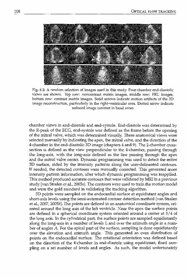
108 OPTICAL FLOW TRACKING

Fig. 6.2: A random selection of images used in this study. Four-chamber end-diastolic views are shown. Top row: noncontrast matrix images, middle row: FRU images, bottom row: contrast matrix images. Solid arrows indicate motion artifacts of the 3D image reconstruction, particularly in the right-ventricular area. Dotted arrow indicate

reduced image contrast in basal areas.

chamber views in end-diastole and end-systole. End-diastole was determined by the R-peak of the ECG, end-systole was defined as the frame before the opening of the mitral valve, which was determined visually. These anatomical views were selected manually by indicating the apex, the mitral valve, and the direction of the 4-chamber in the end-diastolic 3D image (chapters 4 and 9). The 2-chamber cross­section is defined as the view perpendicular to the 4-chamber, passing through the long-axis, with the long-axis defined as the line passing through the apex and the mitral valve center. Dynamic programming was used to detect the entire 3D surface, aided by the intensity patterns along the user-delineated contours. If needed, the detected contours were manually corrected. This generated more intensity pattern information, after which dynamic programming was reapplied. This method produced accurate contours that were validated by MRI in a previous study [van Stralen et al., 2005a]. The contours were used to train the motion model and were the gold standard in validating the tracking algorithm.

3D points were sampled on the endocardial surface at equidistant angles and short-axis levels using the semi-automated contour detection method [van Stralen et al., 2007, 2005b]. The points are defined in an anatomical coordinate system, ori­ented around the long axis of the left ventricle. Near the apex the surface points are defined in a spherical coordinate system oriented around a center at 3 I 4 of the long axis. In the cylindrical part, the surface points are sampled equidistantly along the long-axis in a number of levels L and over the azimuth angle in a num­ber of angles A. For the apical part of the surface, sampling is done equidistantly over the elevation and azimuth angle. This generated an even distribution of points on the endocardial surface. The rotational orientation was defined based on the direction of the 4-chamber in end-diastole using equidistant, fixed sam­pling on a set number of levels and angles. As such, the model unfortunately

6.2 METHODS

did not contain rotational behavior tangential to the endocardial surface, such as twisting of the left ventricle.

Parameter choices

Several parameter choices were needed for optimal functioning of the algorithm. The initial guesses for those parameters were taken from the recent literature. For the image preprocessing step, we relied on the recommendations reported in Siihling et al. [2005] and Danilouchkine et al. [2008]. More accurate tracking results have been observed for ultrasound images that were mildly smoothed (i.e. Gaussian kernel width of cr < 2) prior to optical flow computation [Danilouchkine et al., 2008]. Lindeberg [1998a] showed that image smoothing results in more accu­rate optical flow estimates, because the presence of noise degrades the response of the difterential operators used. Likewise, Baraldi et al. [1996] and Danilouchkine et al. [2008] employed Gaussian filtering prior to optical flow computation in ul­trasound images. For the motion-guided method, we used downsampled data as in van Stralen et al. [2007], because this method generated global motion patterns throughout the whole cardiac cycle. Full resolution data was used for the basic tracking, as this was a purely data-driven method. The choice for the tracking kernel size N appears to be less critical [Yu et al., 2006]. Duan et al. [2008] used 73 voxel ( =4.23mm3) kernel size for tracking, while Yu et al. [2006] used 173 vox­els. We also adhered to the common practice in statistical shape modeling and discarded the 5% least significant modes of variation [Cootes et al., 2001]. The number of vertices for accurate description of the entire myocardial surface can vary between 512 and 1400 [van Assen, 2006, ch. 6],[van Assen et al., 2008], in Bosch et al. [2002], the cardiac boundary in a long-axis view was modeled with 37 landmarks. A = 30 angles and L = 30 levels were used for the motion-guided method, as in van Stralen et al. [2007]. The basic tracking used a more sparse distribution to match the larger kernel size. The initial values for the parameters were experimentally varied and chosen based on the algorithm's performance on twelve noncontrast Matrix sequences, by varying only one parameter each time while keeping the other parameters constant. None of these parameter choices proved to be very critical. The parameter choices based on these experiments are listed in Table 6.1.

Experiments

We performed tracking experiments using the basic Lucas-Kana de approach, the proposed motion-guided approach, and the combination of the two (see section 6.2.5). For segmenting the noncontrast Matrix and FRU images, the motion mod­els were built with the noncontrast Matrix data sets. The models were built in a leave-one-out fashion for the noncontrast Matrix data. All noncontrast Matrix contours were used to build models for tracking in the FRU images. For segment­ing the contrast Matrix images, the models were constructed using contours from the contrast data, also in a leave-one-out fashion.

Point-to-point, point-to-surface, and volume errors were calculated, with re-

109

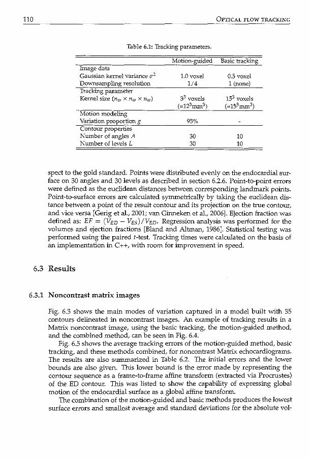
110 OPTICAL FLOW TRACKING

Table 6.1: Tracking parameters.

Motion-guided Basic tracking Image data Gaussian kernel variance Cf2

Downsampling resolution Tracking parameter Kernel size ( nw X nw x nw)

Motion modelmg Variation proportion g Contour properties Number of angles A Number of levels L

1.0 voxel 1/4

33 voxels (=123mm3)

95%

30 30

0.5 voxel 1 (none)

153 voxels (=153mm3)

10 10

spect to the gold standard. Points were distributed evenly on the endocardial sur­face on 30 angles and 30 levels as described in section 6.2.6. Point-to-point errors were defined as the euclidean distances between corresponding landmark points. Point-to-surface errors are calculated symmetrically by taking the euclidean dis­tance between a point of the result contour and its projection on the true contour, and vice versa [Gerig eta!., 2001; van Ginneken et al., 2006]. Ejection fraction was defined as: EF = (VED- VEs)IVED· Regression analysis was performed for the volumes and ejection fractions [Bland and Altman, 1986]. Statistical testing was performed using the paired 1-test. Tracking times were calculated on the basis of an implementation in C++, with room for improvement in speed.

6.3 Results

6.3.1 N oncontrast matrix images

Fig. 6.3 shows the main modes of variation captured in a model built with 35 contours delineated in noncontrast images. An example of tracking results in a Matrix noncontrast image, using the basic tracking, the motion-guided method, and the combined method, can be seen in Fig. 6.4.

Fig. 6.5 shows the average tracking errors of the motion-guided method, basic tracking, and these methods combined, for noncontrast Matrix echocardiograms. The results are also summarized in Table 6.2. The initial errors and the lower bounds are also given. This lower bound is the error made by representing the contour sequence as a frame-to-frame affine transform (extracted via Procrustes) of the ED contour. This was listed to show the capability of expressing global motion of the endocardial surface as a global affine transform.

The combination of the motion-guided and basic methods produces the lowest surface errors and smallest average and standard deviations for the absolute vol-

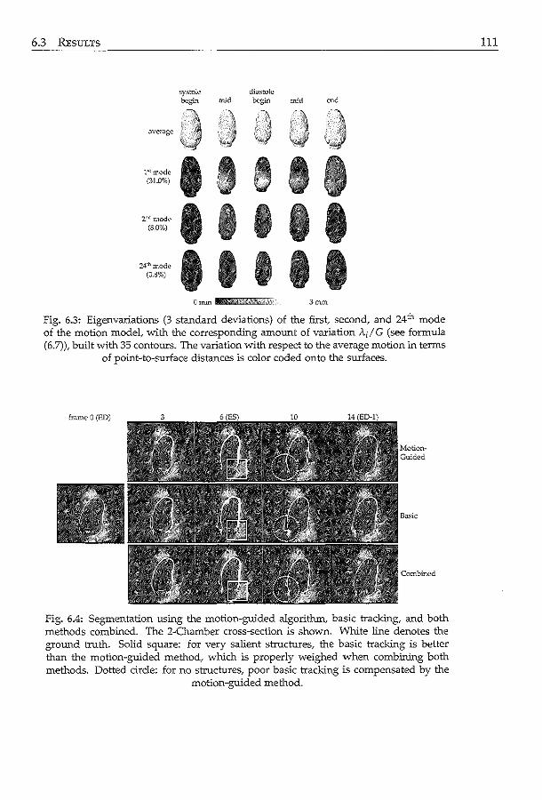
6.3 REsuLTS

systole di;;.stolc - mid begin mid

aver;;~gc

l"'roode I • A I I (31.0%) f/JJ r:J

2"mode 1 1 1 1 1 (8.0%)

,..m2de I I I I I (Q.S,o)

3mm

Fig. 6.3: Eigenvariations (3 standard deviations) of the first~ second, and 24th mode of the motion model, with the corresponding amount of variation Ad G (see formula (6.7)), built with 35 contours. The variation with respect to the average motion in terms

of point-to-surface distances is color coded onto the surfaces.

Fig. 6.4: Segmentation using the motion-guided algorithm, basic tracking, and both methods combined. The 2-Chamber cross-section is shown. White line denotes the ground truth. Solid square: for very salient structures, the basic tracking is better than the motion-guided method, which is properly weighed when combining both methods. Dotted circle: for no structures, poor basic tracking is compensated by the

motion-guided method.

111

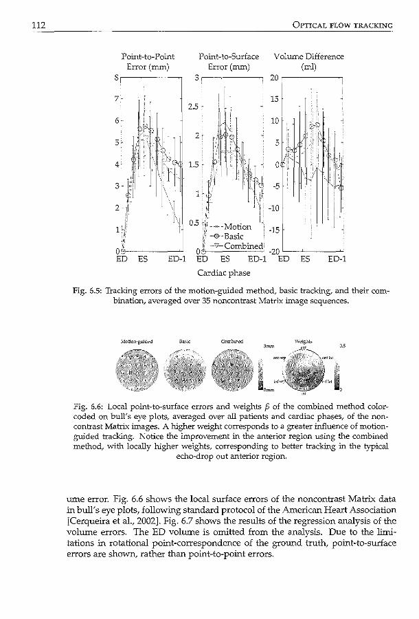
112

Point-to-Point Error (mrn)

8,-------,

,, ''·'

Or~7/,'.' ----------'-' ED ES ED-1

OPTICAL FLOW TRACKING

Point-to-Surface Volume Difference Error (mrn) (ml)

3 20--~------~

15

ES ED-1

Cardiac phase

Fig. 6.5: Tracking errors of the motion-guided method, basic traddng, and their com­bination, averaged over 35 noncontrast Matrix image sequences.

Fig. 6.6: Local point-to-surface errors and weights p of the combined method color­coded on hull's eye plots,. averaged over all patients and cardiac phases, of the non­contrast Matrix images. A higher weight corresponds to a greater influence of motion­guided tracking. Notice the improvement in the anterior region using the combined method, with locally higher weights, corresponding to better tracking in the typical

echo-drop out anterior region.

ume error. Fig. 6.6 shows the local surface errors of the noncontrast Matrix data in bull's eye plots, following standard protocol of the American Heart Association [Cerqueira eta!., 2002]. Fig. 6.7 shows the results of the regression analysis of the volume errors. The ED volume is omitted from the analysis. Due to the limi­tations in rotational point-correspondence of the ground truth, point-to-surface errors are shown, rather than point-to-point errors.

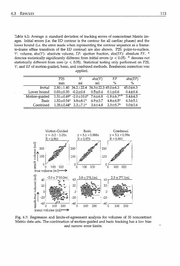
6.3 RESULTS

Table 6.2: Average ± standard deviation of tracking errors of noncontrast Matrix im­ages. Initial errors (i.e. the ED contour is the contour for all cardiac phases) and the lower bound (i.e. the error made when representing the contour sequence as a frame· to-frame affine transform of the ED contour) are also shown. P2S: point-to-surface, V: volume, abs(V): absolute volume, EF: ejection fraction, abs(EF): absolute EF. •· denotes statistically significantly different from .initial errors (p < 0.05). + denotes not statistically different from zero (p < 0.05). Statistical testing only performed on P2S, V, and EF of motion-guided, basic, and combined methods. Bonferroni correction was

applied.

P2S v abs(V) EF abs(EF) mm rnl rnl % %

Initial 2.50±1.40 34.2±22.4 34.3±22.3 45.0±6.3 45.0±6.3 Lower bound 0.83±0.30 -0.2±0.6 0.5±0.4 0.1±0.6 0.4±0.4

Motion-guided 1.51±0.69* -2.0±10.0'" 7.6±6.8 -1.9±6.7'" 5.4±4.3 Basic 1.52=0.54* 3.8±8.1'" 6.9±5.7 4.8±6.5'" 6.3±5.1

Combined 1.35±0.44'' 2.3±7.1'" 5.6±4.8 2.5±5.7* 5.0±3.6

Motion-Guided Basic Combined y"' -3.2 + l.Olx y = 5.1 + 0.98Sx y = 3.1 + 0.99x R = 0.961 R = 0.974 R = 0.981

.§. ?00 I _.~1· 200 I /j200 .

! fo: 1/ 100 t:.k_~~-..Jro: v"--------~ 0 100 200 °o 100 200 0 h-ue volume (ml)--7-

100 200

-_.,2::-.0-_,+:_--:,?*1 0 .Om.l 40- ~0 0

-20 I -40 OL_~_~___j

100 200

Fig. 6.7: Regression and limits-of-agreement analysis for volumes of 35 noncontrast Matrix data sets. The combination of motion-guided and basic tracking has a low bias

and narrow error limits.

113

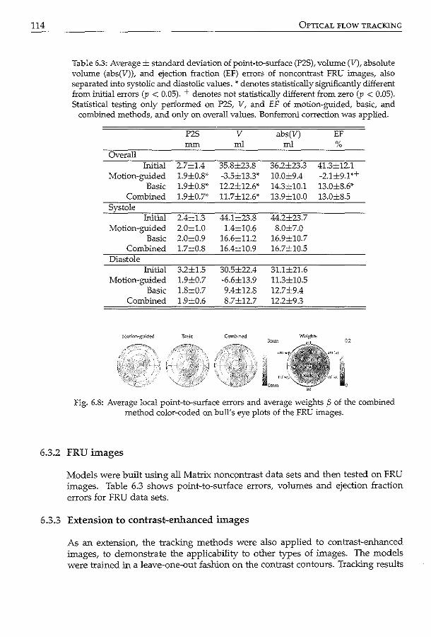
114 OPTICAL FLOW TRACKING

Table 6.3: Average± standard deviation of point-to-surface (P2S), volume (V), absolute volume (abs(V)), and ejection fraction (EF) errors of noncontrast FRU images, also separated IDto systolic and diastolic values.* denotes statistically significantly different from initial errors (p < 0.05). + denotes not statistically different from zero (p < 0.05). Statistical testing only performed on P2S, V, and EF of motion-guided, basic, and

combined methods, and only on overall values. Bonferroni correction was applied.

P2S v abs(V) EF mm ml ml %

Overall Initial 2.7±1.4 35.8±23.8 36.2±23.3 41.3±12.1

Motion-guided 1.9±0.8'· -3.5±13.3' 10.0±9.4 -2.1±9.1'+ Basic 1.9±0.8' 12.2±12.6' 14.3±10.1 13.0±8.6'

Combined 1.9±0.7' 11.7±12.6' 13.9±10.0 13.0±8.5 Systole

Initial 2.4±1.3 44.1±23.8 44.2±23.7 Motion-guided 2.0±1.0 1.4±10.6 8.0±7.0

Basic 2.0±0.9 16.6±11.2 16.9±10.7 Combined 1.7±0.8 16.4±10.9 16.7±10.5

Diastole Initial 3.2±1.5 30.5±22.4 31.1±21.6

Motion-guided 1.9±0.7 -6.6±13.9 11.3±10.5 Basic 1.8±0.7 9.4±12.8 12.7±9.4

Combined 1.9±0.6 8.7±12.7 12.2±9.3

Fig. 6.8: Average local point-to-surface errors and average weights {3 of the combined method color-coded on hull's eye plots of the FRU images.

6.3.2 FRU images

Models were built using all Matrix nonqmtrast data sets and then tested on FRU images. Table 6.3 shows point-to-surface errors, volumes and ejection fraction errors for FRU data sets.

6.3.3 Extension to contrast-enhanced images

As an extension, the tracking methods were also applied to contrast-enhanced images, to demonstrate the applicability to other types of images. The models were trained in a leave-one-out fashion on the contrast contours. Tracking results

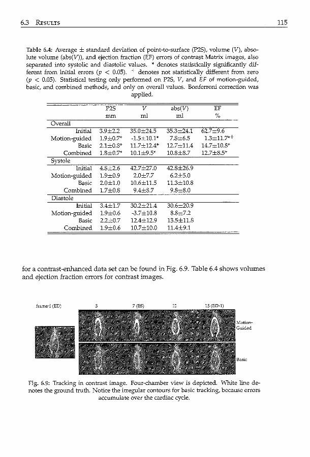
6.3 REsULTS

Table 6.4: Average ± standard deviation of point-to-surface (P2S),. volume (V), abso­lute volume (abs(V)), and ejection fraction (EF) errors of contrast Matrix images, also separated into systolic and diastolic values. * denotes statistically significantly dif­ferent from initial errors (p < 0.05). + denotes not statistically different from zero (p < 0.05). Statistical testing only performed on P2S, V, and EF of motion-guided, basic, and comb:ined methods, and only on overall values. Bonferroni correction was

applied.

P2S v abs(V) EF mm ml ml %

Overall Initial 3.9±2.2 35.0±24.5 35.3±24.1 62.7±9.6

Motion-guided 1.9±0.7'" -1.5±10.1'" 7.8±6.5 1.3±11.7*+ Basic 2.1±0.8* 11.7±12.4'" 12.7±11.4 14.7±10.8*

Combined 1.8±0.7* 10.1±9.5* 10.8±8.7 12.7±8.5' Systole

Initial 4.8±2.6 42.7..:..27.0 42.8±26.9 Motion-guided 1.9±0.9 2.0±7.7 6.2±5.0

Basic 2.0±1.0 10.6±11.5 11.3=10.8 Combined 1.7±0.8 9.4±8.7 9.8±8.0

Diastole Initial 3.4±1.7 30.2±21.4 30.6±20.9

Motion-guided 1.9±0.6 -3.7±10.8 8.8±7.2 Basic 2.2±0.7 12.4±12.9 13.5±11.8

Combined 1.9±0.6 10.7±10.0 11.4±9.1

for a contrast-enhanced data set can be found in Fig. 6.9. Table 6.4 shows volumes and ejection fraction errors for contrast images.

frameO (ED)

Fig. 6.9: Tracking in contrast image. Four-chamber view is depicted. 'White line de­notes the ground truth. Notice the irregular contours for basic tracking, because errors

accumulate over the cardiac cycle.

ns

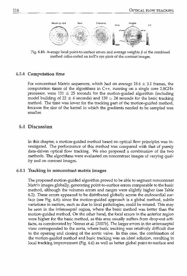
116 OPTICAL FLOW TRACKING

3mm Weights

0.3

1'1+

'' 0

Fig. 6.10: Average local point-to-surface errors and average weights p of the combined method color-coded on buJY s eye plots of the contrast images.

6.3.4 Computation time

For noncontrast Matrix sequences, which had on average 18.6 ± 3.1 frames, the computation times of the algorithms in C++, running on a single core 2.8GHz processor, were 131 ± 25 seconds for the motion-guided algorithm (including model building of 22 ± 6 seconds) and 139 ± 24 seconds for the basic tracking method. The time was lower for the tracking part of the motion-guided method, because the size of the kernel in which the gradients needed to be sampled was smaller.

6.4 Discussion

In this chapter, a motion-guided method based on optical flow principles was in­vestigated. The performance of this method was compared with that of purely data-driven optical flow tracking. We also proposed a combination of the two methods. The algorithms were evaluated on noncontrast images of varying qual­ity and on contrast images.

6.4.1 Tracking in noncontrast matrix images

The proposed motion-guided algorithm proved to be able to segment noncontrast Matrix images globally. generating point-to-surface errors comparable to the basic method, although the volumes errors and ranges were slightly higher (see Table 6.2). These errors appeared to be distributed globally across the endocardial sur­face (see Fig. 6.6); since the motion-guided approach is a global method, subtle variations in motion, such as due to local pathologies, could be missed. This may be seen in the inferoseptal region, where the basic method was better than the motion-guided method. On the other hand, the local errors in the anterior region were higher for the basic method, as this area usually suffers from drop-out arti­facts, as corroborated by Nemes et al. [2007b]. The larger errors in the anteroseptal view corresponded to the aorta, where basic tracking was relatively difficult due to the opening and closing of the aortic valve. In this case, the combination of the motion-guided method and basic tracking was an ideal solution, resulting in local tracking improvement (Fig. 6.6) as well as better global point-to-surface and

6.4 DISCUSSION

volume errors (Table 6.2). While the point-to-point errors may seem relatively high, especially at end­

systole, we would like to stress that the ground truth used did not contain rota­tional components. This may cause the twisting behavior of the left ventricle to be omitted. On the other hand, a data-driven tracking method such as optical flow should be able to detect this rotational behavior, provided that the myocardium is sufficiently visible and not obscured by artifacts. This influences the compari­son between the ground truth and the tracking results in terms of point-to-point errors. This lack of rotational behavior may have had a negative effect on the re­sults of the motion-guided method. While this is a major limitation of the current study, establishing point-correspondence in temporal images is not a trivial task (see section 6.4.5). Therefore, in this study, we must rely more on the point-to­surface and volume errors for judging the merits of our methods.

The average point errors at the end of the cardiac cycle were lower for the motion-guided method than for the basic method (Fig. 6.5). This is due to the inherent temporal continuity of the motion-guided method, so that the point er­rors almost return to their average starting value at the end of the cardiac cycle. Because the basic tracking method was performed on a frame-to-frame basis, er­rors could easily accumulate across the cardiac cycle. This finding can be used to adjust the weights of the combined method to rely more on the motion-guided tracking near the end of the cardiac cycle.

Interestingly, the bias in volume error using basic tracking was larger than for the motion-guided approach (Table 6.2). This 'lagging' behavior is inherent in the Lucas-Kanade solution, as commented by Silltling et al. [2005]. Noisy esti­mates of the image gradients generally lead to an underestimation of the motion [Danilouchkine et al., 2008], so that the contour tends to stay closer to the end­diastolic contour during the cardiac cycle. For the motion-guided method, how­ever, the tracking results will tend to resemble the mean motion instead. Also, since end-systole was synchronized during phase normalization, the detected contour in end-systole should conform to the model's mean contour in that phase. The low ejection fraction bias suggests that this might well be the case (Table 6.2).

117

Tracking in FRU images 6.4.2

For the more challenging FRU images, the motion-guided method was still able to provide good results, especially given the fact that the model was built using contours of Matrix images. Surface errors were comparable; however, the volume errors of the motion-guided method were superior to those of the basic method, especially in systole (see Table 6.3). For the basic method, a larger bias in ejection volume was found, which may be a result of the 'lagging' behavior as discussed in section 6.4.1. This demonstrates the merits of motion-guided tracking in relatively 'difficult' images.

Overall, the tracking results in these images are worse than those in the Ma­trix images. Because the FRU image reconstruction was based on interpolat­ing irregularly spaced 2D images in 3D+ T domain, the frame-to-frame differ­ences in intensity were generally larger than those of the Matrix images. These

118 OPTICAL FLOW TRACKING

large frame-to-frame differences may disturb the brightness constancy assump­tion [Danilouchkine et al., 2008]. Whereas the Matrix data are reconstructed by stitching four adjacent subvolumes [Brekke et al., 2007], the FRU data are re­constructed from irregularly distributed ultrasonic beam lines from several heart cycles. Patient breathing or motion of the ultrasonic probe could result in mo­tion artifacts, that present themselves as irregular edges in the images (see Fig. 6.2). These edges may not necessarily be consistent in time, shifting from frame to frame. The higher errors in the inferoseptal region for the basic tracking cor­respond to a local higher density of these edge artifacts in the images, caused by the presence of the right-ventricular wall (as indicated by arrows in Fig. 6.2).

Also, since motion-artifacts manifest themselves as sharp discontinuities in the FRU images, the saliency weights may be large in those areas (section 6.2.5), resulting in relatively low weights overall (see Fig. 6.10). This may have caused the combined method to falsely rely on the basic tracking, causing the basic tracking and the combined results to be similar. More future research is needed to provide a more suitable combination of both methods.

6.4.3 Extension to contrast images

In this chapter, we also showed the feasibility of applying the motion-guided method to contrast-enhanced images. This is very encouraging, since there are few reports on automatic segmentation in 4D contrast images in the literature. The swirling of the contrast produces highly fluctuating intensity patterns, which makes it challenging for any intensity-based tracking method. The inferior basic tracking results are probably due to the swirling contrast images. The motion­guided method has better point-to-surface and volume errors than the basic meth­od. Also, the bias in ejection fraction is much smaller (see Table 6.4).

The difficulties in tracking the basal segments are reflected in the local sur­face errors of the basic tracking method (Fig. 6.10). Similarly, Oost et al. [2006] reported difficulties in matching their active appearance models to the basal part of the heart in LV angiograms. However, in this case, we think that the attenua­tion of the ultrasound beam due to the echogenic contrast agent causes a lower image contrast further away from the transducer, making tracking more difficult compared with noncontrast images (see Fig. 6.2).

In this study we applied a model which was built using images of one type of equipment (Matrix data) to images with different acquisition settings (FRU data) quite successfully. The idea of using generic models for segmentation tasks is ap­pealing. Previously, Van Assen et al. used a cardiac active shape model built with MR1 data to segment both CT and MR images under various acquisition settings [van Assen et al., 2003, 2006]. This success relies heavily on the fact that the left ventricular appearance is similar in both modalities. Similarly, qualitative results of a motion model built with tagged MR1 for segmenting the left ventricle in ul­trasound were presented in Gerard et al. [2002]. Unfortunately, no quantitative results were available in that paper for comparison (see section 6.4.4). In our case, we were not able to apply the noncontrast motion model to contrast images, be­cause heart morphology is imaged differently in noncontrast and contrast images.

6.4 DISCUSSION

For contrast images, the blood is imaged, whereas for the noncontrast images, the muscular myocardial wall and trabeculae are most apparent. In end-systole, tra­beculae on the inside of the LV contract, so that all blood is squeezed out [Voor­molen and Danilouchkine, 2007]. This is differently visualized in the noncontrast images, resulting in a difference in motion patterns. However, we believe that if these differences can be trained, the motion model can be adapted accordingly. The differences in contour delineation in noncontrast and contrast may also ex­plain why the point and volume errors are higher than those of the noncontrast images, despite the fact that they come from the same patient database.

119

Comparison with other work 6.4.4

Table 6.5 lists the comparative analysis of the point-to-surface and volumetric er­rors achieved by other groups with segmentation algorithms. Due to the vast amount of literature on segmentation, the scope of our comparison is constrained to the most recent work on cardiac ultrasound. Also, as ours is a 3D tracking method, we limit the comparison to automated 3D+time methods with surface and volume errors reported in recent technical papers. Furthermore, comparisons with papers on strain analysis are omitted, as no strain results were available with our method. A distinction was made between segmentation and tracking meth­ods, as ours is a tracking method. The surface and volume errors obtained in this study compares well with the ones reported in the previously published papers. However, since ours is a tracking method, and needs a 3D initialization, the er­rors cannot be entirely compared with those of the segmentation-only papers. A second comment is that the methods of Myronenko et a!. [2007] and Duan et a!. [2008] were evaluated on open chest animal models, of which the images are not contaminated by drop-out artifacts caused by the rib cage (as is the case with in vivo clinical data).

According to Barron eta!. [1994], who tested nine different optical flow algo­rithms including the Horn-Schunck and Lucas-Kanade methods, the latter algo­rithm was the most reliable. Si.ihling eta!. [2005] found that their Lucas-Kanade based method was more accurate for echocardiograms, although Baraldi et a!. [1996] noticed little difference between these two. The difference in results may be explained by the choice of parameters, such as kernel sizes and smoothing constraints. Here, we chose the Lucas-Kanade method because of its computa­tion efficiency. Actually, by combining the Lucas-Kanade solution with a statis­tical motion model, the proposed algorithm also remotely resembles the Horn­Schunck constraint because a globally smooth affine flow along the endocardial boundary was built into the Lucas-Kanade solution. In that sense, the proposed method possibly combines the best of both worlds. This general conclusion agrees with the one reported by Bruhn et a!. [2005], who combined the Horn-Schunck and Lucas-Kanade formulations and obtained better tracking results, especially in noisy images.

Several papers have been published on block matching versus optical flow. Malpica et a!. [2004] compared block-matching and the Lucas-Kanade approach, and concluded that the latter was best for contrast echocardiograms. Veronesi

120 OPTICAL FLOW TRACKING

et a!. [2006] used both methods consecutively to detect the long-axis of the left ventricle in echocardiographic sequences. Combinations of smart block-matching [Behar et a!., 2004; Lingmaru et a!., 2008] and optical flow may be used to further refine the motion-guided approach.

6.4.5 Limitations

A major limitation of this study is the lack of rotational point correspondence in the motion model, due to the limitation in the semi-automated contour detection program that was used to generate training contours. Establishing point corre­spondence in ultrasound images is not a trivial task. In this study, a ground truth of the torsion of the left ventricle was not available. For in vivo patient imaging, point correspondence can be obtained for example via MRI tagging [Florack et al., 2007; Gerard eta!., 2002]. Such data was not available in this study. For ultra­sound images, point correspondence may be achieved theoretically using dense annotations of endocardial landmarks, which is a time consuming job. Another option is using speckle tracking [Helle-Valle et a!., 2005], although this poses a challenge in clinical 3D images due to current hardware limitations in frame rate.

Since the motion model was built with one affine transform per frame, the resulting model only showed global patterns of motion. This is a major limitation of this study. However, the global errors made by modeling the contour sequence as an frame-to-frame affine transformation of the ED contour were quite small (lower bound in Table 6.2). Also, by using this global affine transform, spuri­ous, noisy motion patterns are removed, whlch may arise from inconsistencies in the training contours. In this study, we proposed to do a refinement using basic tracking to achieve more accurate results locally. This basic tracking may also be enhanced using affine-motion representation [Siihling et a!., 2005], higher order optical flow terms [Otte and Nagel, 1995], or replaced by smart template matching teclmiques, e.g. using features [Yeung et al., 1998a]. Another way is to build more local models, e.g. using only a part of the cardiac phase or left ventricular region. We have performed some experiments using separate local models and encoun­tered difficulties in areas with shadowing and in the near-field of the transducer. A way to deal with this is to identify these areas, either manually or automatically, and exclude these from the tracking. Here, the gradient norm of the images was used to determine roughly if image regions contained salient structures, but more sophisticated methods can be developed. However, automated artifact detection for ultrasound images is not a trivial problem and requires further investigation.

The current implementation relies on manual identification of the end-systolic phase in the image. This could be replaced by a reliable automatic method, based on ECG. More time points may be added, such as the end of the rapid-filling phase in diastole [Perperidis eta!., 2005]. However, more manual interaction should be avoided.

An inherent limitation of model-based methods is that the training sets should comprise the expected variation of the underlying anatomical organ. To demon­strate the versatility of the proposed approach, the image data included a mixed population of normal and abnormal heart function. Still, good results were ob-

6.5 CONCLUSION

tained in this study, despite this large variability. For a more detailed look at the differences between tracking in normal and abnormal sequences, one would have to obtain many more patients in all kinds of pathologies, for example in an extensive clinical trial. Previously, we have performed feasibility studies on classifying localized pathologies in echocardiographic sequences using statistical shape models (Bosch et al. [2005], chapter 8). However, the data sets for building and validating the model in these studies were considerably larger. Moreover, the models represented only 2D motion. Obviously, separate models for different pathologies can be built and applied to the images, taking the best performing model (e.g. with the lowest intensity tracking error) as the final result. Therefore, the question about the suitability of the proposed approach for the purposes of classification of the local heart abnormalities remains open and definitely requires further investigation.

121

Extensions 6.4.6

The current motion model was derived from LV contours, however, it would be interesting to augment this model with texture information. One way to do this is to learn models of brightness variations from one frame to the next. Obviously, this requires the images to be acquired using similar equipment. If these patterns can be identified, the motion parameters and brightness variation parameters can be resolved in an iterative scheme, using the found motion parameters to update the brightness variation parameters and vice versa.

Conclusion 6.5

A tracking method for delineating contours in 3D+time left ventricular echocar­diograms was proposed. A pre-trained model of cardiac motion was fitted to the images to be segmented, using an optical-flow based formulation. For good qual­ity noncontrast images, optimal results were obtained using a smart combination of a local tracker with the proposed motion-guided method. For data sets of chal­lenging image quality, the motion-guided method provided good estimates of left ventricular volume and ejection fraction. Encouraging results were obtained in contrast-enhanced images.

>-'

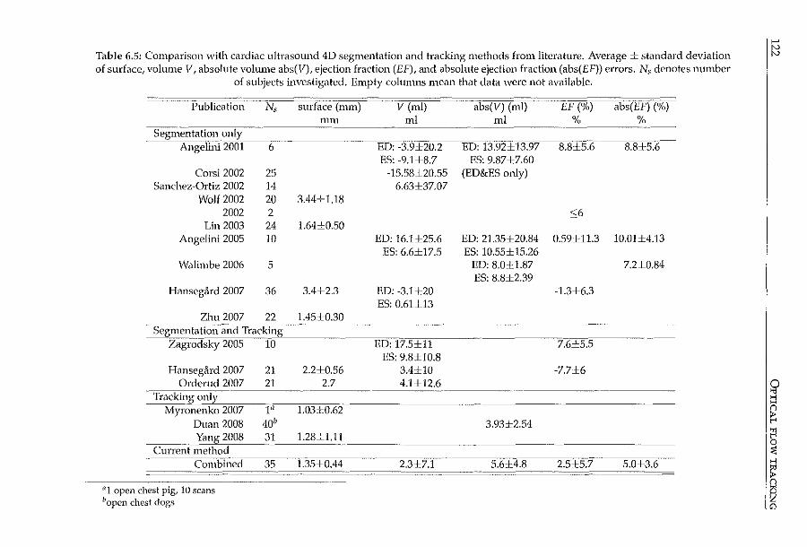
Table 6.5: Comparison with cardiac ultrasound 4D segmentation and tracking methods from literature. Average± standard deviation it::l of surface, volume V, absolute volume abs(F), ejection fraction (EF), and absolute ejection fraction (abs(EF)) errors. Ns denotes number

of subjects investigated. Empty columns mean that data ·were not available.

Publication Ns surface (mm) V (ml) abs(V) (ml) EF (%) abs(EF) (%) rnm ml ml % %

Segnlei1tation only ···---

Angelini 2001 6 ED: -3.9±20.2 ED: 13.92±13.97 8.8±5.6- 8.8±5.6 ES: -9.1±8.7 ES: 9.87±7.60

Corsi 2002 25 -15.58±20.55 (ED&ES only) Sanchez~Ortiz 2002 14 6.63±37.07

Wolf2002 20 3.44±1.18 2002 2 <:;6

Lin 2003 24 1.64±0.50 Angelini 2005 10 ED: 16.1±25.6 ED: 21.35±20.84 0.59:UL3 10.01±4.13

ES: 6.6±17.5 ES: 10.55± 15.26 Walimbe 2006 5 ED: 8.01:1.87 7.2±0.84

ES: 8.8±2.39 Hansegard 2007 36 3.4±2.3 ED: -3.1±20 -1.3±6.3

ES: 0.61±13 Zhu 2007 22 1.451:0.30

Segmentation ail-d Tracking .. ____

Zagrodsky 2005 ib ED: 17.5±11 7.6±5.5 ES: 9.8±10.8

Hanseg<lrd 2007 21 2.2±0.56 3.4±10 -7.7±6 Orderud 2007 21 2.7 4.1±12.6 0

Tracking only " >-l _,,- H

Myronenko 2007 J:il 1.03±0.62 n

Duan 2008 40" 3.93±2.54 ~ Yang 2008 31 1.28±1.11 fl

··--- 0 CurreilTmethod :<

Combiilect 35 1.35±0.44 2.3±7.1 5.6J:4.8 2.5cl:5.7 5.0±3.6 ~ n

11 1 open chest pig, 10 scans

I~ 11open chest dogs

(7:)\. cc_ ! ;<

\_____/ \'-;·"' •'-'

i1

·~~0

0• //~ Probabilistic 0J ~\ framework for 1

/\ • • \..___)\

improving tracking ~']&(]/ in artifact-prone images ~ L-

Echocardiography is a commonly-used, safe, and noninvasive method for assessing cardiac dysfunction and related coronary artery disease. The analysis of echocardio­grams, whether visual or automated, has traditionally been hampered by the presence of ultrasound artifacts, which obscure the moving myocardial wall. In this chapter, a probabilistic framework for trackill.g the endocardial surface .in 3D ultrasound images is proposed. Artifacts which obscure the myocardium are detected in order to improve the quality of cardiac boundary segmentation. The expectation-maximization algo­rithm is applied in a stationary and cardiac motion frame-of-reference, and weights are derived accordingly. The weights are integrated with an optical-flow based con­tour tracking method, which incorporates prior knowledge via a statistical model of cardiac motion. Evaluation on 35 3D echocardiographic sequences shows that this weighed tracking method significantly improves the tracking results. In conclusion, the proposed weights are able to reduce the influence of artifacts, resulting in a more accurate quantitative analysis.

Submitted a~: Probabilistic fr.un~work foe improving tracking in Mlifact-pron~ 3D ~choc;udiogr.uns K Y.E. kung, M.G. D.:milouchkine, M. van StrJkn, N. de Jong, ;md J.G. Bo5Ch.

124 PROBABILISTIC TRACKING

7.1 Introduction

7.1.1 Artifacts in cardiac ultrasound

Echocardiography is a commonly-used, fast, and relatively inexpensive imag­ing modality for assessing left ventricular dysfunction and underlying coronary artery disease. 2D echocardiography is used in many hospitals across the world to obtain parameters of cardiac function noninvasively. In recent years, 3D echocar­diography has undergone many technological advances and is becoming increas­ingly popular. By imaging the whole left ventricle in 3D, many options become available for analyzing the heart's true 3D behavior. All this makes ultrasound a very attractive imaging modality for cardiac diagnosis.

Despite these advantages, there are also some drawbacks to ultrasound imag­ing. Echocardiograms may be difficult to interpret, so that a long learning curve is required. The reason is that the images may be contaminated by speckle noise, and often contain ultrasound artifacts. Common anomalies in echocardiograrns are side-lobes artifacts, reverberations, shadowing, and near-field clutter [Feigen­baum eta!., 2005, p. 29-32].

Side-lobes of the main, central ultrasound beam may cause echoes coming from the side-lobe areas to appear as if they come from the main beam [Cobbold, 2007, p. 438]. This results in an arched 'edge' in the image, and can be clearly seen if the object in the side-lobe has a strong reflection. Lesser degrees of the side­lobe artifact increase the general noise level of the image. Reverberations occur when the sound beam bounces back and forth between reflectors in the imaged area before it is received by the transducer. This artifact appears as one or more echo targets directly behind the reflector [Hedrick and Peterson, 1995]. Typically, reverberation and side-lobe artifacts that originate from a fixed reflector (e.g. a rib)-will not move with the motion of the heart. A more troublesome artifact is shadowing. Shadowing is caused by objects in the ultrasound path which cause high reflections or attenuation, leaving an area of low intensity beyond [Nelson et a!., 2000]. In transthoracic cardiac images, this is usually caused by the rib cage, which prevents the imaging of the myocardium (causing the so-called drop­out regions). This is especially problematic in 3D echocardiography, because the size of the transducer is generally speaking larger than that of the 2D transducer, making it harder to image between the ribs. Near-field clutter arises from rever­berations of high-amplitude signals close to the transducer [Feigenbaum et al., 2005, p. 32]. This hampers the imaging of objects in this area, and is particularly noticeable in echocardiograms acquired from the apical window, where the near­field clutter often obscures the left ventricular apex. Fig. 7.1 shows examples of typical ultrasound artifacts. For accurate visual and quantitative assessment of the heart, it is highly desirable to identify such artifacts. Areas where the cardiac wall is obscured by such artifacts should be detected and dealt with differently in the analysis.

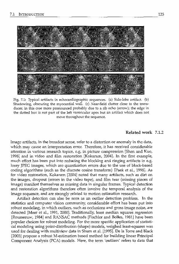
7.1 INTRODUCTION

Fig. 7.1: Typical artifacts in echocardiographic sequences. (a) Side-lobe artifact. (b) Shadowing, obscuring the myocardial wall. (c) Near-field clutter close to the trans­ducer, in this case more pronounced probably due to a rib echo (arrow); the edge in the dotted box is not part of the left ventricular apex but an artifact which does not

move tl-rroughout the sequence.

125

Related work 7.1.2

Image artifacts, in the broadest sense, refer to a distortion or anomaly in the data, which may cause an interpretation error. Therefore, it has received considerable attention in various research topics, e.g. in pictuTe compression [Shen and Kuo, 1998] and in video and fiim restoration [Kokaram, 2004]. ln the first example, much effort has been put into reducing the blocking and ringing artifacts in e.g. lossy JPEG images, which are quantization errors due to the use of block-based coding algorithms (such as the discrete cosine transform) [Paek et al., 1998]. As for video restoration, Kokaram [2004] noted that many artifacts, such as dirt on the images, dropout (errors in the video tape), and fiim tear (missing pieces of image) manifest themselves as missing data in singular frames. Typical detection and restoration algorithms therefore often involve the temporal analysis of the image sequence, and are strongly related to motion estimation research.

Artifact detection can also be seen as an outlier detection problem. ln the statistics and computer vision community, considerable effort has been put into robust modeling, in which outliers, such as occlusions and gross image noise, are detected [Meer et al., 1991, 2000]. Traditionally, least median squares regression [Rousseeuw, 1984] and RANSAC methods [Fischler and Bolles, 1981] have been popular choices for robust modeling. For the more specific application of statisti­cal modeling using point-distribution (shape) models, weighed least-squares was used for dealing with multiview data in Shum et al. [1995]. De !a Torre and Black [2003] propose a robust M-estimation based method for building linear Principal Component Analysis (PCA) models. Here, the term 'outliers' refers to data that

126 PROBABILISTIC TRACKING

does not conform to the assumed statistical model. Recently, such methods have been extended to matching statistical models more robustly. For example, Rogers and Graham [2002] formulated M-estimator and random sampling methods for active shape models. Kaus et al. [2004] used a feature model instead, obtained by classification of the intensity values, to guide statistical model based segmen­tation. Lekadir et al. [2007] proposed a geometric constraint, based on the ratio of inter-landmark distances, to detect outliers during both model building and matching. Likewise, robust methods have been proposed for active appearance models [Gross et al., 2004]. In particular, Beichel et al. [2005] developed a ro­bust matching method using the mean shift algorithm for segmenting X-ray data, which were occluded e.g. by surgical implants.

In Computer Tomography (CT) and Magnetic Resonance (MR) imaging, much work on artifact reduction consists of correcting motion artifacts due to patient breathing and variations in the heart rate. In MR imaging, respiratory artifacts, which cause blurring of the images [Hedley and Yan, 1992], can be limited by breath holding [Bogaert et al., 1995], or more advanced navigator-echo methods [Firmin and Keegan, 2001]. Many reports can also be found on correcting image non-uniformities, caused either by inhomogeneous radio-frequency fields [Had­jidemetriou et al., 2009] or by surface coils which have a nonuniform spatial sen­sitivity [Belaroussi et al., 2006; Lai and Ming, 2003]. The latter artifact affects the imaging of the apex of the heart: since the apex is closer to the body surface and thus also to the coil, it may appear as a bright region so that other structures are obscured. Recently, image processing methods have been introduced, which make use of image registration [Comte et al., 2004; Danilouchkine et al., 2005; Gupta et al., 2003; Stegmann et al., 2005]. For CT, patient motion and heart beat variation may cause streaks in the reconstructed images. This can be reduced by shortening the acquisition time using multidetector-row systems (multislice CT) [Kopp et al., 2004] and dual-source systems [Roberts et al., 2008]. Postprocessing methods also exist; e.g. Manzke et al. [2004] developed a retrospectively gated reconstruction algorithm which takes into account the heart rate variations.

For removing ultrasonnd artifactsf much effort involving hardware improve­ments has been described in the literature, such as different pulsing schemes and frequencies, and reduction of the transducer footprint. For example, second har­monic imaging not only offers spatial resolution improvements and reduced side­lobes, but also reduces the energy at the very near-field, resulting in less near-field clutter [Duck, 2002]. Coded excitation is a popular method for improving signal to noise ratio [Takeuchi, 1979]. To improve the overall visibility of the myocardium in echocardiograms, contrast agents are often employed [Nemes et al., 2007b]. This may help the diagnosis of patients whose images have a low signal-to-noise ratio.

Several reports can be found on image processing techniques for artifact de­tection in ultrasound. Stationary clutter rejection methods have been developed mostly for color Doppler flow imaging [Bjaerum et al., 2002; Cloutier et al., 2003; Yoo et al., 2003]. For identifying reverberations in normal ultrasound images, Duarte et al. [2003] presented an algorithm based on the comparison of power spectra and time-of-flight. Bylund et al. [2005] proposed to detect reverberation artifacts from a static reflector using quadrature filters. These were then removed

7.1 INTRODUCTION

using 2D+time Wiener filtering. A method to remove near-field noise was re­ported by Hozumi et al. [1998]. They assume that the noise in the near-field is generated by steady reflectors (such as ribs and intercostal muscles), whereas the echo from moving myocardium is dynamic. Therefore, they apply a high-pass filter over the radio-frequency signal over time, similar to clutter removal in color Doppler imaging. Zwirn and Akselrod [2006] proposed to classify the time inten­sity curves of echocardiographic image sequences. They looked at the temporal average and standard deviation of the intensity at each pixel of the image, and classified them into stationary clutter, moving cardiac wall, and blood. This was done by fitting three Gaussian histograms to the distributions of the average and standard deviations throughout the image. Most of the above methods show that the temporal information is of great importance in detecting artifacts in echocar­diographic images.

127

Study goal 7.1.3

In this chapter, we propose a framework for improving the tracking of endo­cardial borders in 3D echocardiographic sequences, by detecting areas in which the myocardium is obscured by typical artifacts such as shadowing, near-field clutter, and static reverberations. The goal is to automatically recognize these ar­tifacts and suppress their influence on endocardial border tracking, to ultimately improve the quality of the segmentation. To accomplish this, we incorporate tem­poral intensity information from the images into an optical-flow-based tracking framework.

Previously, we have proposed an optical-flow-based method for tracking left ventricular endocardial borders throughout the cardiac cycle (chapter 6). The method consists of a global tracker which is guided by a statistical cardiac mo­tion model, followed by a refinement using purely data-driven tracking. The idea is that the 'motion-guided tracker' estimates the global motion of the myocar­dial wall on the basis of the statistically learned patterns of heart contraction. Subsequently, this global estimate is refined using a local optical-flow tracker, as described by Lucas and Kanade [1981]. To improve this tracking framework, it makes sense to only apply the local refinement in salient areas, which can be tracked accurately.

In the previous study (chapter 6), salient areas were detected using a simple measure defined using the intensity gradient norm. In ultrasound images, higher gradients could be found at the interface between the left ventricular cavity and the myocardial wall, if the latter is clearly visible, whereas if the myocardium is obscured by shadowing, the gradients would be low. However, high gradients can also be found in the near-field region and in areas with static reverberations artifacts. In this chapter, we propose a probabilistic framework to also deal with the latter artifacts.

The method we have opted for is inspired by the work of Jepson et al. [2003], in which an expectation-maximization (EM) approach was used to categorize tem­poral features of image sequences. They incorporated this into a framework for tracking people in video sequences. This approach resembles the work of Stauffer

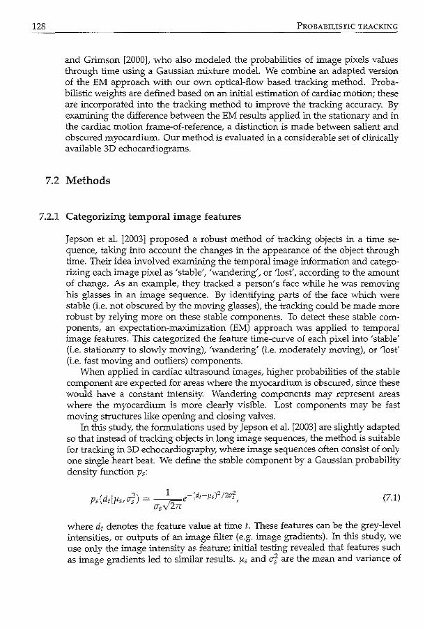
128 PROBABILISTIC TRACKING

and Grimson [2000], who also modeled the probabilities of image pixels values through time using a Gaussian mixture model. We combine an adapted version of the EM approach with our own optical-flow based tracking method. Proba­bilistic weights are defined based on an initial estimation of cardiac motion; these are incorporated into the tracking method to improve the tracking accuracy. By examining the difference between the EM results applied in the stationary and in the cardiac motion frame-of-reference, a distinction is made between salient and obscured myocardium. Our method is evaluated in a considerable set of clinically available 3D echocardiograms.

7.2 Methods

7.2.1 Categorizing temporal image features

Jepson et al. [2003] proposed a robust method of tracking objects in a time se­quence, taking into account the changes in the appearance of the object through time. Their idea involved examining the temporal image information and catego­rizing each image pixel as 'stable', 'wandering', or 'lost', according to the amount of change. As an example, they tracked a person's face while he was removing his glasses in an image sequence. By identifying parts of the face which were stable (i.e. not obscured by the moving glasses), the tracking could be made more robust by relying more on these stable components. To detect these stable com­ponents, an expectation-maximization (EM) approach was applied to temporal image features. This categorized the feature time-curve of each pixel into 'stable' (i.e. stationary to slowly moving), 'wandering' (i.e. moderately moving), or 'lost' (i.e. fast moving and outliers) components.

When applied in cardiac ultrasound images, higher probabilities of the stable component are expected for areas where the myocardium is obscured, since these would have a constant intensity. Wandering components may represent areas where the myocardium is more clearly visible. Lost components may be fast moving structures like opening and closing valves.

In this study, the formulations used by Jepson et al. [2003] are slightly adapted so that instead of tracking objects in long image sequences, the method is suitable for tracking in 3D echocardiography, where image sequences often consist of only one single heart beat. We define the stable component by a Gaussian probability density function p5 :

P.(d I" cT') = _l_e-(d,-p,)'l2o'f !> t rs, s CTsV2TC , (7.1)

where dt denotes the feature value at time t. These features can be the grey-level intensities, or outputs of an image filter (e.g. image gradients). In this study, we use only the image intensity as feature; initial testing revealed that features such as imao-e cradients led to similar results. "s and a; are the mean and variance of o o r· "

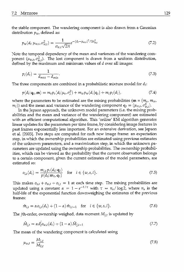
7.2 METHODS

the stable component. The wandering component is also drawn from a Gaussian distribution Pw• defined as:

1 (d )2;o ' Pw(dtlflw_t.o;,,,) = e- ,-~w.r -a-;;,,, !Tw_tV2ii

(7.2)

Note the temporal dependency of the mean and variances of the wandering com­ponent (flw,t. a;,_,). The lost component is drawn from a uniform distribution, defined by the maximum and minimum values of d over all images:

1 Pl(d,) = d -d .

max mm (7.3)

The tluee components are combined in a probabilistic mixture model for dt:

(7.4)

where the parameters to be estimated are the mixing probabilities (m = ( m,, mw, m1)l and the mean and variance of the wandering component q, = (flw,t. cr;,_,).

In the Jepson approach, the unknown model parameters (i.e. the mixing prob­abilities and the mean and variance of the wandering component) are estimated with an efficient computational algorithm. This 'online' EM algorithm generates linear updates for the parameters per time frame, by considering image features in past frames exponentially less important. For an extensive derivation, see Jepson et aL [2003]. Two steps are computed for each new image frame: an expectation step, in which the ownership probabilities are estimated using previous estimates of the unknown parameters, and a maximization step, in which the unknown pa­rameters are updated using the ownership probabilities. The ownership probabil­ities, which can be viewed as the probability that the current observation belongs to a certain component, given the current estimates of the model parameters, are estimated as:

for iE{w,s,l}. (7.5)

This makes o,_~ + Ow_t + 01,1 = 1 at each time step. The mixing probabilities are updated using a constant IX = 1- e-l/r with T = n,/ log2, where n, is the half-life of the exponential function downweighing the estimates of the previous frames:

mi,t=IXOi,t(dt)+(1-1X)mi,t-l for iE{w,s,l}.

The jth-order, ownership weighed, data moment Mj,t is updated by

Mj,t = IXd{ow,t(dt) + (1-IX) Mj_t-l

The mean of the wandering component is calculated using

Mu l'wt = --'

' Mo,t

(7.6)

(7.7)

(7.8)

129

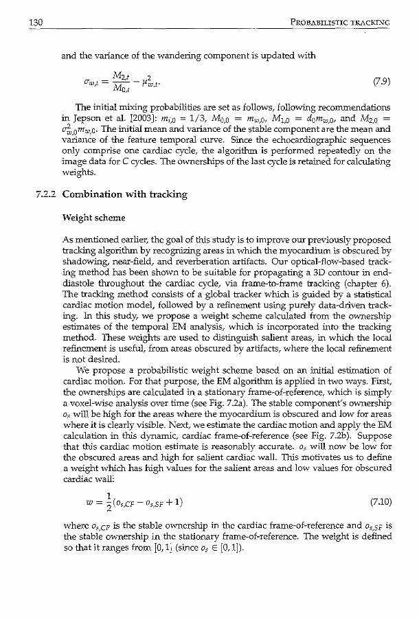
130 PROBABILISTIC TRACKING

and the variance of the wandering component is updated with

(7.9)

The initial mixing probabilities are set as follows, following recommendations in Jepson et a!. [2003]: m;,o = 1/3, Mo.o = mw,o. M1,0 = domw,O• and Mz.o = cr;,_0mw,O· The initial mean and variance of the stable component are the mean and variance of the feature temporal curve. Since the echocardiographic sequences only comprise one cardiac cycle, the algorithm is performed repeatedly on the image data for C cycles. The ownerships of the last cycle is retained for calculating weights.

7.2.2 Combination with tracking

Weight scheme

As mentioned earlier, the goal of this study is to improve our previously proposed tracking algorithm by recognizing areas in which the myocardium is obscured by shadowing, near-field, and reverberation artifacts. Our optical-flow-based track­ing method has been shown to be suitable for propagating a 3D contour in end­diastole throughout the cardiac cycle, via frame-to-frame tracking (chapter 6). The tracking method consists of a global tracker which is guided by a statistical cardiac motion model, followed by a refinement using purely data-driven track­ing. In this study, we propose a weight scheme calculated from the ownership estimates of the temporal EM analysis, which is incorporated into the tracking method. These weights are used to distinguish salient areas, in which the local refinement is useful, from areas obs=ed by artifacts, where the local refinement is not desired.

We propose a probabilistic weight scheme based on an initial estimation of cardiac motion. For that purpose, the EM algorithm is applied in two ways. First, the ownerships are calculated in a stationary frame-of-reference, which is simply a voxel-wise analysis over time (see Fig. 7.2a). The stable component's ownership o5 will be high for the areas where the myocardium is obscured and low for areas where it is clearly visible. Next, we estimate the cardiac motion and apply the EM calculation in this dynamic, cardiac frame-of-reference (see Fig. 7.2b). Suppose that this cardiac motion estimate is reasonably accurate. o5 will now be low for the obscured areas and high for salient cardiac wall. This motivates us to define a weight which has high values for the salient areas and low values for obscured cardiac wall:

(7.10)

where Os,CF is the stable ownership in the cardiac frame-of-reference and Os,SF is the stable ownership in the stationary frame-of-reference. The weight is defined so that it ranges from [0, 1] (since o5 E [0, 1 ]).

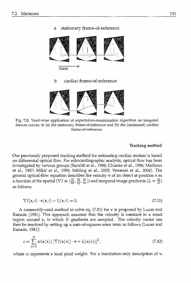
7.2 METHODS 131

a stationary frame-of-reference

time

b cardiac frame-of-reference

Fig. 7.2: Voxel-wise application of expectation-maximization algorithm on temporal feature curves, in (a) the stationary frame-of-reference and (b) the (estimated) cardiac

frame-of-reference.

Tracking method

Our previously proposed tracking method for estimating cardiac motion is based on differential optical flow. For echocardiographic analysis, optical flow has been investigated by various groups [Baraldi et al., 1996; Chunke et aL, 1996; Mailloux et aL, 1987; Mikic et aL, 1998; SUhling et aL, 2005; Veronesi et aL, 2006]. The general optical-flow equation describes the velocity v of an object at position x as

a function of the spatial (vi= (M, ~~'~))and temporal image gradients Ut = Ml as follows:

\7I(x,t) ·v(x,t) +It(x,t) = 0. (7.11)

A commonly-used method to solve eq. (7.11) for v is proposed by Lucas and Kanade [1981]. This approach assumes that the velocity is constant in a small region around x, in which N gradients are sampled. The velocity vector can then be resolved by setting up a sum-of-squares error term as follows [Lucas and Kanade, 1981]:

N

E = I; w(x(n)) [vi(x(n)) · v+ I,(x(n))f, (7.12) n=l

where w represents a local pixel weight. For a translation-only description of v,

132 PROBABILISTIC TRACKING

this can be solved by differentiating eq. (7.12) with respect to each translation component v = ( v, Vy, Vz), and equating the result to zero.

In the previous study, we proposed a method to estimate the global cardiac motion, called motion-guided tracking (chapter 6). This method involves modi­fying the general optical flow equation by embedding a trained statistical cardiac motion model. The motion model is obtained by applying Principal Component Analysis (PCA) on frame-to-frame affine transforms throughout the whole cardiac cycle, similar to the approach used in active shape and active appearance models [Cootes et al., 2001]. These transforms are calculated using Procrustes analysis on a set of training contours. The statistical model is embedded in the optical flow equation by substituting the velocity term with the PCA model, resulting in a modified equation which relates the spatiotemporal image gradients with the PCA model parameters. To track an end-diastolic contour throughout the cardiac cycle, the image gradients are gathered from all image frame-pairs, after which the modified equation is resolved for the PCA model parameters. These parameters are converted back into frame-to-frame affine transforms, which, in turn, are used to transform the end-diastolic contour throughout the heart cy­cle. Since the model parameters are resolved for the whole image and all cardiac phases at once; the resulting segmentation is global, time continuous, and more robust to local anomalies. However, this means that the local tracking results in salient areas, which are easy to track, can still be improved upon. Therefore, we use a basic tracker to refine the results locally, at the contour positions estimated by the motion-guided method. This basic tracker is the standard Lucas-Kanade optical-flow method, as described above [Lucas and Kanade, 1981]. Starting at end-diastole, each contour point is tracked throughout the cardiac cycle, using the results of the motion-guided method as an initial estimate. The position x1 of a contour point at time t is then defined as:

t yt-1 yt-1 yO yO ( 0) X = BT 0 MG 0 ... 0 BT 0 MG X I (7.13)

where Y~y1 is the estimated transform of the basic tracker from frame t- 1 to t, Y MG is the transform of the motion-guided method, and superscript 0 denotes the end-diastolic frame.

Integrating weights with tracking

The EM-weights are incorporated into this tracking scheme in two ways. First, the EM-weights are used to refine the cardiac motion estimation by inserting them as w(x(n)) into the sum-of-squares term (eq. (7.12)) for both the motion-guided and basic tracking methods. Second, the transform of the basic tracker is weighed, so that the salient cardiac wall depends more on the basic tracking. The basic transforms, which are frame-to-frame translations, are weighed as:

YBT,weigl"d (x) = w(x)YBr(x) = ( w(x)vx(x), w(x)vy(x), w(x)vz (x)) . (7.14)

The proposed EM-weight-based tracking algorithm is as follows:

7.2 METHODS 133

Algorithm 7.1 EM-weight-based tracking algorithm.

1. Estimate cardiac motion (section 7.2.2) 2. Estimate EM ownerships in stationary frame-of-reference 3. Estimate EM ownerships in cardiac motion frame-of-reference 4. Combine ownerships into weights (eq. (7.10)) 5. Re-estimate cardiac motion using weights (section 7.2.2)

Experimental details 7.2.3

Data description

To test the performance of the proposed segmentation method, 3D echocardio­graphic sequences were acquired of the left ventricle in patients referred for stress echocardiography. Only images obtained in the rest stage were analyzed. Thirty­five data sets were acquired with a Philips Sonos 7500 system (Philips Medical Systems, Best, The Netherlands), equipped with an X4 matrix array transducer. Typical spatial dimensions were 160 x 144 x 208 voxels with 1mm x 1mm x 0.7mm resolution. The 3D data set comprised 4 electrocardiographically gated pyramidal subvolumes. Twenty of these patients underwent coronary angiogra­phy: 6 patients had no significant vessel disease, 8 patients had one-vessel disease (2 in the left-anterior-descending (LAD) coronary artery region, 4 in the right­coronary-artery (RCA) region, 2 in the left-circumflex-artery (LCX) region), 3 pa­tients had two-vessel disease (LCX and RCA, LAD and RCA, LAD and LCX) and 3 patients had three-vessel disease. The study was approved by the institutional review board, and all patients gave informed consent.

Contour delineation

Left ventricular 3D contours were needed for training the PCA model, as initial­ization in the 3D end-diastolic image, and as the ground truth in the validation. Full-cycle endocardial borders were drawn with a previously developed semi­automated method, based on pattern matching and dynamic programming [van Stralen et aL, 2005a]. In short, the contour was delineated in the four-chamber and two-chamber views in end-diastole and end-systole. End-diastole was determined by the R-peak of the ECG, end-systole was defined as the frame before the open­ing of the mitral valve, which was determined visually. These anatomical views were selected manually by indicating the apex, the mitral valve, and the direction of the four-chamber in the end-diastolic 3D image (chapter 4). The two-chamber cross-section is defined as the view perpendicular to the four-chamber, passing through the long-axis, with the long-axis defined as the line passing through the apex and the mitral valve center. Dynamic programming was used to detect the entire 3D surface, aided by the intensity patterns along the user-delineated con­tours. If needed, the detected contours were manually corrected. This generated more intensity pattern information, after which dynamic programming was reap­plied. This method produced accurate contours that were validated by MRl in a

134 PROBABILISTIC TRACKING

previous study [van Stralen et al., 2005a]. 3D points were sampled on the endo­cardial surface at equidistant angles and short-axis levels.

Experiments

The motion-guided and the basic tracking methods were applied consecutively according to the description in section 7.2.2. The motion models were tested in a leave-one-out fashion: 34 sequences were used to build the model, which is then applied to the remaining sequence. This is repeated for all data sets.

Point-to-surface and volume errors were calculated, with respect to the gold standard. Ejection fraction was defined as: EF = (Vw - VEs) /Vw, with Vw denoting the volume in end-diastole and VEs denoting the volume in end-systole. Statistical testing was performed using the paired t-test. The difference between tracking with and without the proposed weights is investigated.

Also, we compared the results of the probabilistic tracking framework with our previous gradient-based weight scheme, as outlined in detail in chapter 6. The gradient norm II V Ill was evaluated at each contour point and linear scaling is applied:

w- llviii-IIviiimin (7_15) - llviiimax-llviiimin'

where llviiimin was the minimum and llviiimax was the maximum gradient norm in the whole image.

7.3 Results

Fig. 7.3 shows the stable, wandering, and lost ownerships, in the stationary and cardiac frames-of-reference. The resulting weights are also shown. Examples of images with artifacts and the weight images are displayed in Fig. 7.4. Fig. 7.5 shows the weights in two frames at end-systole, where the opening of the mitral valve can be seen. An example of tracking can be seen in Fig. 7.6.

Fig. 7.7 shows the point-to-surface and volume errors. Three lines are shown, denoting the tracking method without saliency weights, with the previously pro­posed gradient-based weights, and with the currently proposed probabilistic weights, showing the improvement in tracking accuracy using the current method.

Quantitative tracking results are summarized in Table 7.1. Averages and stan­dard deviations are taken over the whole cardiac cycle, omitting the ED phase.

7.4 Discussion

In this chapter, a method was proposed to distinguish between obscured and salient moving myocardium in echocardiograms. The method categorized fea-

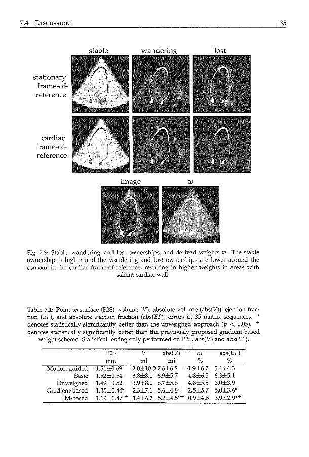
7.4 DISCUSSION

stationary frame-of­reference

cardiac frame-of­reference

fig. 7.3: Stable, wandering, and lost ownerships, and derived weights w. The stable ownership is higher and the wandering and lost ownerships are lower aronnd the contour in the cardiac frame-of-reference, resulting in higher weights in areas with

salient cardiac wall.

Table 7.1: Point-to-surface (P2S), volume (V), absolute volume (abs(V)), ejection frac­tion (EF), and absolute ejection fraction (abs(EF)) errors in 35 matrix sequences. •· denotes statistically significantly better than the unweighed approach (p < 0.05). + denotes statistically significantly better than the previously proposed gradient-based

weight scheme. Statistical testing only performed on P2S, abs(V) and abs(EF).

P2S v abs(V) EF abs(EF) mm ml ml % %

Motion-guided 1.51±0.69 -2.0±10.0 7.6±6.8 -1.9±6.7 5.4±4.3 Basic 1.52±0.54 3.8±8.1 6.9±5.7 4.8±6.5 6.3±5.1

Unweighed 1.49±0.52 3.9±8.0 6.7±5.8 4.8±5.5 6.0±3.9 Gradient-based 1.35±0.44* 2.3±7.1 5.6±4.8* 2.5±5.7 5.0±3.6*

EM-based 1.19±0.47''~ 1.4±6.7 5.2±4.5*T 0.9±4.8 3.9±2.9*+

135

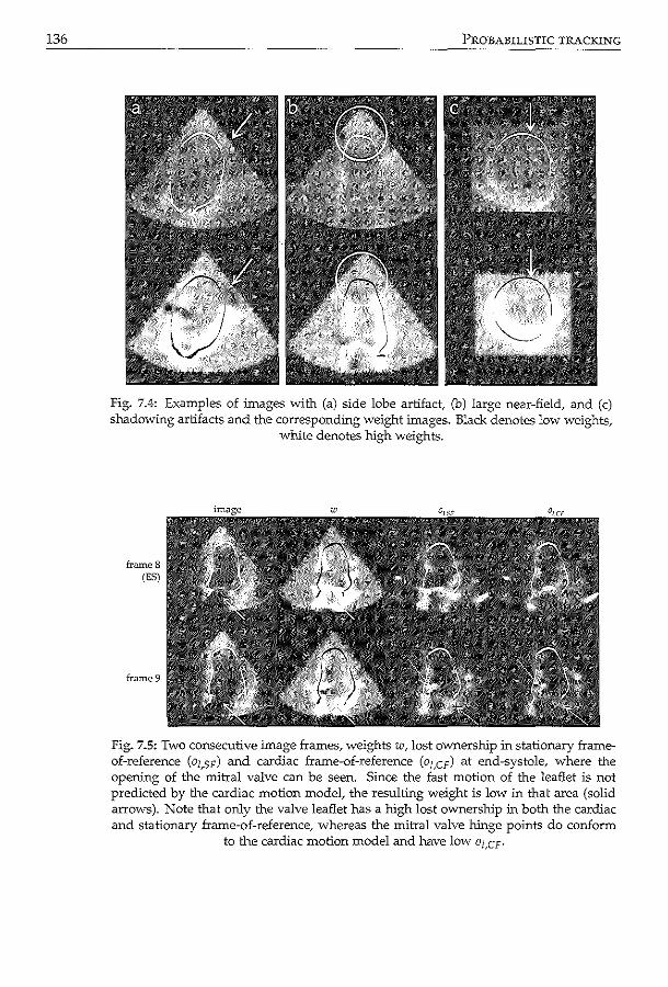
136 PROBABILISTIC TRACKING

Fig. 7.4: Examples of images with (a) side lobe artifact, (b) large near-field, and (c) shadowing artifacts and the corresponding weight images. Black denotes low weights,

white denotes high weights.

frame 8 (ES)

frame9

Fig. 7.5: Two consecutive image frames, weights w, lost ovvnership in stationary frame­of-reference (oz,sF) and cardiac frame-of-reference (oz,cF) at end-systole, where the opeWng of the mitral valve can be seen. Since the fast motion of the leaflet is not predicted by the cardiac motion model, the resulting weight is low in that area (solid arrows). Note that only the valve leaflet has a high lost ownership :in both the cardiac and stationary frame-of-reference, whereas the mitral valve hinge points do conform

to the cardiac motion model and have low ol,CF·

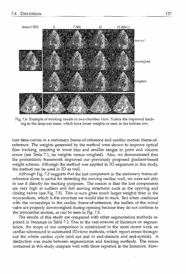
7.4 DISCUSSION

&ameO (ED)

Fig. 7.6: Example of tracking results in tvvo-chamber view. Notice the improved track­ing in the drop-out areas, which have lower weights as seen in the bottom row.

ture time-curves in a stationary frame-of-reference and cardiac motion frame-of­reference. The weights generated by the method were shown to improve optical flow tracking, resulting in lower bias and smaller ranges in point and volume errors (see Table 7.1, no weights versus weighed). Also, we demonstrated that the probabilistic framework improved our previously proposed gradient-based weight scheme. Although the method was applied in 3D sequences in this study, the method can be used in 2D as well.

Although Fig. 7.3 suggests that the lost component in the stationary frame-of­reference alone is useful for detecting the moving cardiac wall, we were not able to use it directly for tracking purposes. The reason is that the lost components are very high at outliers and fast moving structures such as the opening and closing valves (see Fig. 7.5). This in turn gives much larger weights than in the myocardium, which is the structure we would like to track. But when combined with the ownerships in the cardiac frame-of-reference, the leaflets of the mitral valve are properly down weighed during opening because they do not conform to the myocardial motion, as can be seen in Fig. 7.5.

The results of this study are compared with other segmentation methods re­ported in literature in Table 7.2. Due to the vast amount of literature on segmen­tation, the scope of our comparison is constrained to the most recent work on cardiac ultrasound in automated 3D+time methods, which report errors through­out the whole cardiac cycle (and not just in end-diastole and end-systole). A distinction was made between segmentation and tracking methods. The errors contained in this study compare well with those reported in the literature. How-

137

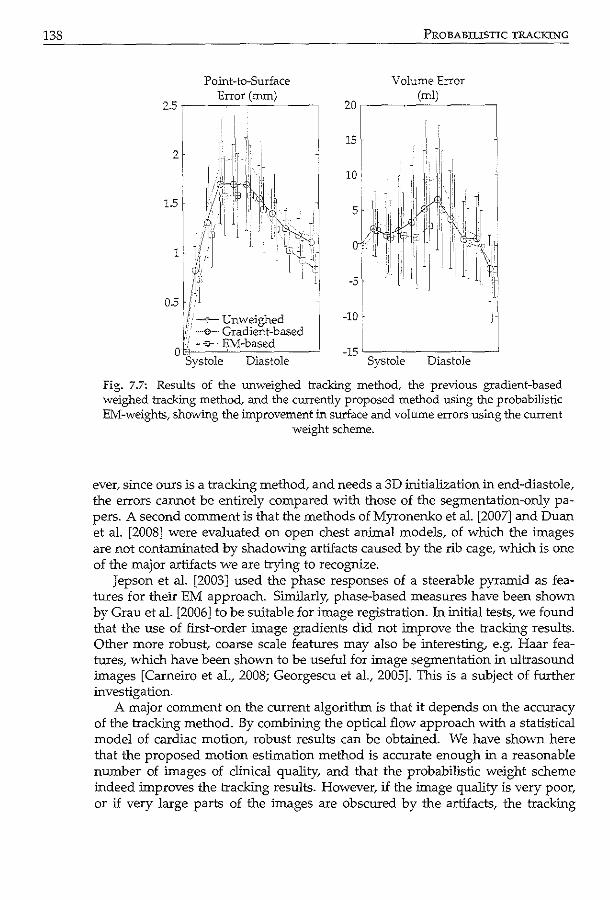
138 PROBABUISTIC TRACKING

Volume Error Point-to-Surface Error (nun)

25r, ------~~----, (ml)

20~----~~----_,

Fig. 7.7: Results of the unweighed tracking method, the previous gradient-based weighed tracking method, and the currently proposed method using the probabilistic EM-weights, showing the improvement in S'Ul"face and volume errors using the current

weight scheme.

ever, since ours is a tracking method, and needs a 3D initialization in end-diastole, the errors cannot be entirely compared with those of the segmentation-only pa­pers. A second comment is that the methods of Myronenko et al. [2007] and Duan et a!. [2008] were evaluated on open chest animal models, of which the images are not contaminated by shadowing artifacts caused by the rib cage, which is one of the major artifacts we are trying to recognize.

Jepson et al. [2003] used the phase responses of a steerable pyramid as fea­tures for their EM approach. Similarly, phase-based measures have been shown by Grau et al. [2006] to be suitable for image registration. In initial tests, we found that the use of first-order image gradients did not improve the tracking results. Other more robust, coarse scale features may also be interesting, e.g. Haar fea­tures, which have been shown to be useful for image segmentation in ultrasound images [Carneiro et a!., 2008; Georgescu et al., 2005]. This is a subject of further investigation.

A major comment on the current algorithm is that it depends on the accuracy of the tracking method. By combining the optical flow approach with a statistical model of cardiac motion, robust results can be obtained. We have shown here that the proposed motion estimation method is accurate enough in a reasonable number of images of clinical quality, and that the probabilistic weight scheme indeed improves the tracking results. However, if the image quality is very poor, or if very large parts of the images are obscured by the artifacts, the tracking

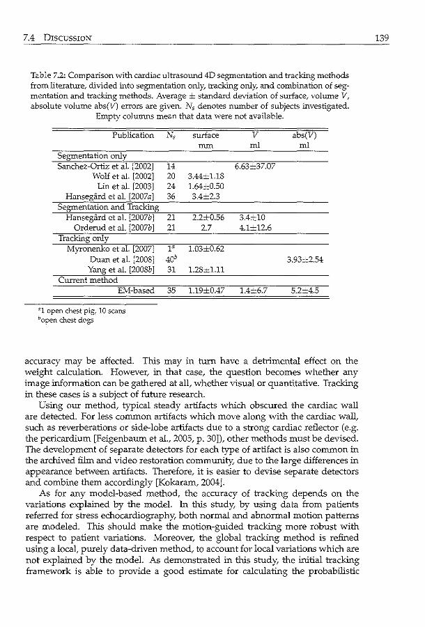
7.4 DISCUSSION

Table 7.2: Comparison with cardiac ultrasormd 4D segmentation and tracking methods from literature,. divided into segmentation only, tracking only,. and combination of seg­mentation and tracking methods. Average ± standard deviation of surface, volume V, absolute volume abs(V) errors are given. N5 denotes number of subjects investigated.

Empty colunms mean that data were not available.

Publication Ns surface v abs(V) mm ml ml

Segmentation only Sanchez-Ortiz et al. [2002] 14 6.63±37.07

Wolf et al. [2002] 20 3.44±1.18 Lin et al. [2003] 24 1.64±0.50

Hansegard et al. [2007 a] 36 3.4±2.3 Segmentation and Tracking

Hansegard et al. [2007b] 21 2.2±0.56 3.4±10 Orderud et al. [2007b] 21 2.7 4.1±12.6

Tracking only Myronenko et al. [2007] 1a 1.03±0.62

Duan et al. [2008] 40b 3.93±2.54 Yang et al. [2008b] 31 1.28=1-11

Current method EM-based 35 1.19±0.47 1.4±6.7 5.2±4.5

a1 open chest pig, 10 scans bopen chest dogs

accuracy may be affected. This may in turn have a detrimental effect on the weight calculation. However, in that case, the question becomes whether any image information can be gathered at all, whether visual or quantitative. Tracking in these cases is a subject of future research.

Using our method, typical steady artifacts which obscured the cardiac wall are detected. For less common artifacts which move along with the cardiac wall, such as reverberations or side-lobe artifacts due to a strong cardiac reflector (e.g. the pericardium [Feigenbaum eta!., 2005, p. 30]), other methods must be devised. The development of separate detectors for each type of artifact is also common in the archived film and video restoration community, due to the large differences in appearance between artifacts. Therefore, it is easier to devise separate detectors and combine them accordingly [Kokararn, 2004].

As for any model-based method, the accuracy of tracking depends on the variations explained by the model. In this study, by using data from patients referred for stress echocardiography, both normal and abnormal motion patterns are modeled. This should make the motion-guided tracking more robust with respect to patient variations. Moreover, the global tracking method is refined using a local, purely data-driven method, to account for local variations which are not explained by the model. As demonstrated in this study, the initial tracking framework is able to provide a good estimate for calculating the probabilistic

139

140 PROBABILISTIC TRACKING

weights, in spite of the motion variations.

7.5 Conclusion

A probabilistic weight scheme was proposed for distinguishing between salient and obscured myocardium in 3D ultrasound images for improving endocardial border tracking. Expectation-maximization was applied in a stationary and car­diac motion frame-of-reference. Thls weight scheme was shown to improve track­ing of left ventricular borders in a considerable number of patient data. Based on these promising results, we think that this method shows great potential in improving quantitative analysis in 3D echocardiograms.

/7~~ ~~ / \. I \ I'',

I ·~ \'-;~ I '''-..__.)

' ,'~

~~ Segmental 0 ~~J r, wall motion 8,----,\ j ·~.·· 1 .fi . . ~ j_/\ " ~ • c ass1 cation using - 8"',_;( V

compact shape descriptors ~-~ In this chapter~ we investigate whether parametric shape representations of endocar­dial contours, obtained with principal component analysis (PCA) and the orthomax criterion, provide compact descriptors for classifying segmental left ventricular wall motion. Endocardial contours were delineated in left ventricular echocardiograms from 129 patients. Parametric models of these shapes were built with PCA and subse­quently rotated using the orthomax criterion, producing models with local variations. Shape parameters of this localized model were used to predict the presence of wall motion abnormalities, as determined by expert visual wall motion scoring. Best re­sults were obtained using the varimax criterion and full variance models. "Whereas traditional PCA models needed 8.0::::::3.0 parameters to classify segmental wall motion; only 5.1±3.2 parameters were needed using the orthomax rotated models (p < 0.05) to achieve similar classification accuracy. The classification space also was better be­haved. To conclude, orthomax rotation generates more local parameters, which are successful in reducing the complexity of wall motion classification. Since pathologies are typically spatially localized; many medical applications :involving local classifica­tion should benefit from orthomax parameterizations.

@A..;....;ociJ.tion of Uniwrsity R.:!diologists. Re>printcd, with permission, from: Scgmcnbl W.ill. Motion Oassification in Echoc.udiogr.uns using: Compact Sh:.tpc Descriptors K.Y.E. Leung .md J.G. Bosch Acad RJ.diol2008; 15(11}; 1416-24.

142 WALL MOTION CLASSIFICATION

8.1 Introduction

Coronary artery diseases are a major cause of death in the westem world. There­fore, detection of wall-motion abnormalities of the left ventricle (LV), widely ac­cepted as predictors for these diseases, is of great clinical importance. Echocar­diographic examination is often used for diagnosing these wall-motion abnormal­ities, because of the speed of acquisition, the high spatial and temporal resolution, and the relatively low cost of the technique. A well-established method is stress echocardiography, which compares the LV wall-motion in images acquired at dif­ferent stages of stress (i.e. elevated to the maximum workload for the heart mus­cle) [Marwick, 2003]. However, since the images are often evaluated visually, a quantitative and objective measure of wall-motion is still lacking. To obtain such quantitative measures, automated analysis of LV wall motion may be preferred to currently visual, therefore subjective, assessments.

Various quantitative measures have been proposed to assess wall-motion in the literature [Thomas and Popovic, 2006]. Methods such as acoustic quantifi­cation and color kinesis [Mor-Avi et a!., 1997] observe the backscatter of the ultrasonic signal to measure the endocardial motion. Tissue Doppler imaging [Armstrong et a!., 2000] generates measurements of velocity, displacement, and strain/ strain-rate values. These values can also be obtained using image-based speckle-tracking methods [Helle-Valle et a!., 2005], which are becoming increas­ingly popular. Other image-based methods use manual or automated delineations of the endocardial border to assess e.g. regional volumes, which may be of help in quantifying wall-motion [Walimbe et al., 2007].

Methods have also been proposed to automatically detect wall-motion abnor­malities in echocardiograms. Assmann et a!. [1993] proposed to measure wall­motion using regional ejection fraction, area reduction, and fractional shorten­ing, based on endocardial contours. Frouin eta!. [2004] proposed factor analysis to separate the image-intensity time-curves into a 'constant' and a 'contraction­relaxation' factor, to distinguish between different levels of wall-motion. Aoued et al. [2005] applied principal component analysis to strain and strain-rate time­curves. A distance measure was proposed, which expresses the distance between a patient's time-curve and a model of healthy subjects. A special classifier was developed by Fung et a!. [2005] to distinguish between normal and abnormal hearts. Previously, we have suggested using point-distribution models of con­tour sequences in two-dimensional echocardiograms for automated classification of wall-motion abnormalities [Bosch eta!., 2005].

The goal of this study is to evaluate a new automated classification approach for detecting local wall-motion abnormalities. Building on our previous work, the wall-motion parameters are derived from contour sequences of the left ven­tricle [Bosch et a!., 2005]. Point-distribution models with localized variations are obtained with orthomax rotations. The parameters are used to classify segmental wall-motion.

8.2 MATERIALS AND METHODS 143

Materials and methods 8.2

Stress echo and visual wall motion scoring 8.2.1

Stress echo is a commonly used diagnostic technique for assessing LV dysfunc­tion and underlying coronary disease [Marwick, 2003]. This technique consists of acquiring echocardiographic images of the left ventricle when the patient is at rest and at stress (maximum workload for the cardiac muscle). By studying the regional motion patterns of the LV wall, myocardial tissue functionality can be diagnosed. Deteriorating contractility in one or more segments in stress is a sign of local ischemia, associated with a stenosis in the corresponding coronary artery.

The wall motion is assessed visually by assigning a qualitative score to each segment. Different scoring systems are in use; the data in this chapter use a four­point system (0: normokinesia, 1: hypokinesia; 2: akinesia; 3: dyskinesia) and 13 segments [Nijland et al., 2002]. Since each qualitative score is associated with a numeric value, semiquantitative results can be calculated, such as the total score of all segments. However, because the scoring is performed visually, the work is time-consuming and the scoring may suffer from intraobserver and interobserver variabilities [Hoffmann et al., 1996]. Development of an automatic method for classifying wall-motion which emulates visual wall motion scoring, is therefore highly desirable.

Analysis of endocardial contours via shape models 8.2.2

Previously, we have proposed using shape models for classifying LV wall motion automatically [Bosch et al., 2005]. Shape models, or point-distribution-models, are parametric representations of a set of shapes [Coates et al., 2001]. These models are usually built using Principal Component Analysis (PCA). This technique gen­erates a statistical representation of the global shape variations encountered in the input data, e.g. LV endocardial contours of a set of patients. This allows a shape, represented by spatial point-coordinates concatenated in a vector x, to be accurately approximated by a limited number of shape parameters, or modes, concatenated in a vector b:

x=x+Pb, (8.1)

where x is the average shape, and P is the eigenvector matrix. Typically, the number of shape modes is similar to the number of input training samples. Any new shape can be projected to this model using the pseudoinverse (P-1) of the eigenvector matrix: b ""p-1(x- x).

The modeling technique was extended to time sequences of echocardiograrns [Bosch et al., 2002].ln this way, the model comprised variations in LV wall-motion patterns across a group of patients. The complex motion pattern of the left ven­tricle could then be accurately described with these shape modes.

The shape modes were then used to classify global clinical parameters (e.g. LV volume) and local parameters (e.g. visual wall-motion scores) [Bosch et al., 2005].

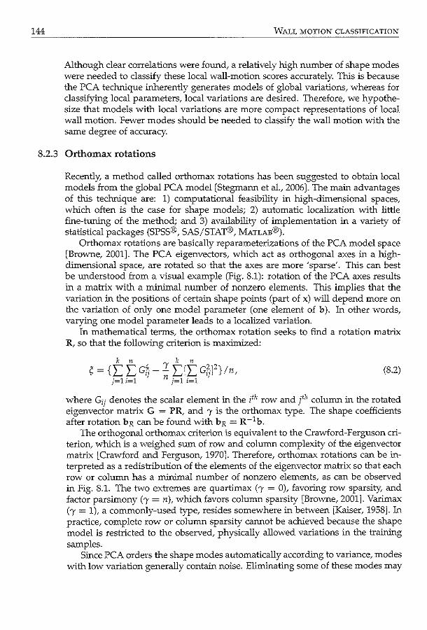
144 WALL MOTION CLASSIFICATION

Although clear correlations were found, a relatively high number of shape modes were needed to classify these local wall-motion scores accurately. This is because the PCA technique inherently generates models of global variations, whereas for classifying local parameters, local variations are desired. Therefore, we hypothe­size that models with local variations are more compact representations of local wall motion. Fewer modes should be needed to classify the wall motion with the same degree of accuracy.

8.2.3 Orthomax rotations

Recently, a method called orthomax rotations has been suggested to obtain local models from the global PCA model [Stegmann et al., 2006]. The main advantages of this technique are: 1) computational feasibility in high-dimensional spaces, which often is the case for shape models; 2) automatic localization with little fine-tuning of the method; and 3) availability of implementation in a variety of statistical packages (SPSS®, SAS/STAT®, MATLAB®).

Orthomax rotations are basically reparameterizations of the PCA model space [Browne, 2001]. The PCA eigenvectors, which act as orthogonal axes in a high­dimensional space, are rotated so that the axes are more ~sparse'. This can best be understood from a visual example (Fig. 8.1): rotation of the PCA axes results in a matrix with a minimal number of nonzero elements. This implies that the variation in the positions of certain shape points (part of x) will depend more on the variation of only one model parameter (one element of b). In other words, varying one model parameter leads to a localized variation.

In mathematical terms, the orthomax rotation seeks to find a rotation matrix R, so that the following criterion is maximized:

(8.2)

where G;i denotes the scalar element in the ;th row and j'h column in the rotated eigenvector matrix G = PR, and ')' is the orthomax type. The shape coefficients after rotation bR can be found with bR = R-1b.

The orthogonal orthomax criterion is equivalent to the Crawford-Ferguson cri­terion, which is a weighed sum of row and column complexity of the eigenvector matrix [Crawford and Ferguson, 1970]. Therefore, orthomax rotations can be in­terpreted as a redistribution of the elements of the eigenvector matrix so that each row or column has a minimal number of nonzero elements, as can be observed in Fig. 8.1. The two extremes are quartimax (/' = 0), favoring row sparsity, and factor parsimony(')'= n), which favors column sparsity [Browne, 2001]. Varirnax (')' = 1), a commonly-used type, resides somewhere in between [Kaiser, 1958]. In practice, complete row or column sparsity cannot be achieved because the shape model is restricted to the observed, physically allowed variations in the training samples.

Since PCA orders the shape modes automatically according to variance, modes with low variation generally contain noise. Eliminating some of these modes may

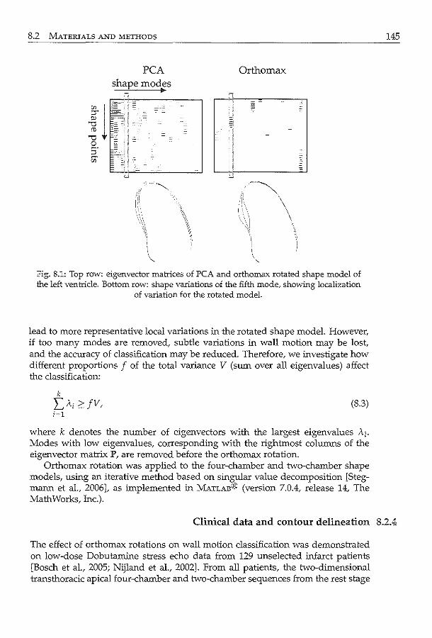
8.2 MATERIALS AND METHODS

PCA shape modes

Orthomax

-~.

\

Fig. 8.1: Top row: eigenvector matrices of PCA and orthomax rotated shape model of the left ventricle. Bottom row: shape variations of the fifth mode, showing localization

of variation for the rotated model.

lead to more representative local variations in the rotated shape model. However, if too many modes are removed, subtle variations in wall motion may be lost, and the accuracy of classification may be reduced. Therefore, we investigate how different proportions f of the total variance V (sum over all eigenvalues) affect the classification:

k

L"i ?JV, (8.3) i=l

where k denotes the number of eigenvectors with the largest eigenvalues Ai. Modes with low eigenvalues, corresponding with the rightmost columns of the eigenvector matrix P, are removed before the orthomax rotation.

Orthomax rotation was applied to the four-chamber and two-chamber shape models, using an iterative method based on singular value decomposition [Steg­mann et al., 2006], as implemented in MATLAB® (version 7.0.4, release 14, The Math Works, Inc.).

145

Clinical data and contour delineation 8.2.4

The effect of orthomax rotations on wall motion classification was demonstrated on low-dose Dobutarnine stress echo data from 129 unselected infarct patients [Bosch et al., 2005; Nijland et al., 2002]. From all patients, the two-dimensional transthoracic apical four-chamber and two-chamber sequences from the rest stage

146

Apical Four-Chamber ApicJl

WALL MOTION CLASSIFICATION

Apical Two-Chamber I

Coron;1ry Territories

c:Juo !:<<,,j LCX

l::::t:t:~:::±fRCA

fig. 8.2: LV segments in four-chamber and tvvo-chamber views (LAD = left anterior descending artery, LCX = left circumflex artery, RCA = right coronary artery).

were available for shape modeling (Fig. 8.2). Each temporal sequence was normal­ized to 16 frames, of which the first and last frame corresponded to end-diastole (ED) and the ninth frame to end-systole (ES). Endocardial borders were delin­eated independent of the visual wall motion scoring, using a semi-automated tracing program (ECHO-CMS system, MEDIS Medical Imaging Systems, Leiden, the Netherlands [Bosch et al., 1998]). The contour in each frame was modeled by 37 points.

For training of the PCA model, the x andy coordinates of these contour points of all frames were concatenated in x. This was carried out for all training patient data sets. These vectors were the input to the PCA.

8.2.5 Wall motion classification

Two classification experiments were performed, denoted as the 'TRN L-1-0' and the 'TST' case. The total data set was split randomly into a training set (TR.t'J) of 65 patients and a testing set (TST) of 64 patients. Shape models of the four-chamber and two-chamber were built with the training set, as in our previous work [Bosch et al., 2005]. Shape parameters b and bR were calculated for all data sets. In the 'TR.t'J L-1-0' case, a leave-one-out approach was used, where the classifier was trained on the TRN set except for one sample and tested with that sample. This process was then repeated for all TRN samples. In the 'TST' situation, the classifier was trained on the whole TRN set and then tested on all TST cases. This resembled classification in the real-world: both shape model and classifier were trained with a limited training set and tested on completely 'new' shapes.

For single segments and combinations of two to five segments, a distinction was made between normal (summed score= 0) and abnormal (summed score> 0) motion. For combinations of more than five segments, in which many scores were summed, this distinction would result in very biased classes (because the patient set contained only infarct patients and no normals). Therefore, a distinc­tion was made between mild (summed score ::; 3) and severe (summed score >

8.3 REsULTS

3) wall motion abnormalities. This distinction in scores was used as the response (dependent) variables in the classification.

To classify the wall motion abnormalities, Linear Discriminant Analysis (LDA) was used. This classifier searches for a linear combination of the shape parameters that provides the best discrimination between classes [Webb, 2002]. In the param­eter space spanned by the shape parameters, this discriminant can be observed as a hyperplane, separating the normal-motion and abnormal-motion classes: L,j~1 cx;b; + cxo = 0, where q is the number of shape parameters in the classifi­cation space. Linear discriminant analysis was performed using the statistical package SPSS (v. 11.0.1, 2001). Shape parameters were added automatically by the classifier using the 'stepwise' option and the 'unexplained variance' criterion, so that an optimal subset q of the k shape parameters were selected that best discriminate between normal and abnormal motion.

To investigate whether the normal and abnormal classes were better separated in the orthomax parameter space than the original PCA space, cluster measures were computed. After the classifier has selected a subset q of the k shape parame­ters which best predicts normal or abnormal wall motion, these q parameters of a particular patient can be seen as a point in the q-dimensional classification space. Ideally, for a linear classifier such as LDA, points of the normal class should form a compact cloud (or cluster), completely separated from the point-cluster of the abnormal class. A common measure of cluster compactness is the within-class scatter matrix Sw, whereas the between-class scatter matrix S B is often used to describe cluster separation. A measure of overall cluster quality is the ratio J of the trace of the two scatter matrices ([Webb, 2002], p. 311): J = tr(SB) /tr(Sw ).

147

Results 8.3

Orthomax rotations 8.3.1

Orthomax rotations were applied to four-chamber (4C) and two-chamber (2C) shape models. Whereas PCA shape modes are ordered according to variance, thus exhibiting global variations in the first modes, orthomax modes show lo­cal variations in most modes (see Fig. 8.3). Since the whole cardiac cycle was modeled, the variations were localized along the spatial as well as the temporal extent.

Orthomax criteria 8.3.2

Shape parameters were used to predict the presence of wall motion abnormali­ties for each individual LV segment. Significantly fewer orthomax modes were needed than PCA modes, without compromising classification accuracy (i.e. the proportion of segments correctly classified as normal or abnormal, see Table 8.1). The varimax criterion needed the least number of modes.

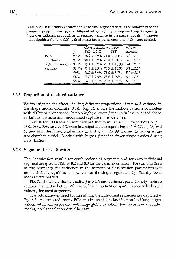
148 WALL MOTION CLASSIFICATION

Table 8.1: Classification accuracy of individual segments versus the number of shape parameters used (mean±sd) for different orthomax criteria, averaged over 9 segments. f denotes different proportions of retained variance in the shape models. * denotes

that significantly (p < 0.05, paired t-test) fewer parameters than PCA were needed.

Classification accuracy #Para-

f TRNL-1-0 TST meters. PCA 99.9% 88.9 ±5.9% 74.0 _:_ 9.4% 8.0±3.0 quartimax 99.9% 90.1 ±5.2% 75.4 ± 9.8% 5.6±3.9* factor parsimony 99.9% 89.4±5.7% 76.3 ± 10.3% 5.4= 3.2* varimax 99.9% 91.1 ±4.5% 76.5 ± 10.5% 5.1 ±3.2'"

99% 88.9 ±5.9% 76.0 ± 8.7% 5.7±3.3* 98% 87.7±7.0% 75.8 ± 9.5% 6.4±3.5 95% 86.3± 6.1% 76.3 ± 9.0% 6.6±3.7

8.3.3 Proportion of retained variance

We investigated the effect of using different proportions of retained variance in the shape model (formula (8.3)). Fig. 8.3 shows the motion patterns of models with different proportions. Interestingly, a lower f results in less localized shape variations, because each mode must capture more variation.

Results for classification accuracy are shown in Table 8.1. Proportions of f = 95%, 98%, 99% and 99.9% were investigated, corresponding to k = 27, 40, 48, and 63 modes in the four-chamber model, and to k = 25, 38, 46, and 62 modes in the two-chamber model. Models with higher f needed fewer shape modes during classification.

8.3.4 Segmental classification

The classification results for combinations of segments and for each individual segment are given in Tables 8.2 and 8.3 for the varimax criterion. For combinations of two segments, the reduction in the number of classification parameters was not statistically significant. However, for the single segments, significantly fewer modes were needed.

Fig. 8.4 shows the cluster quality J in PCA and varimax space. Clearly, varimax rotation resulted in better definition of the classification space, as shown by higher values J for most segments.

The actual modes used for classifying the individual segments are depicted in Fig. 8.5. As expected, many PCA modes used for classification had large eigen­values, which corresponded with large global variation. For the orthomax rotated modes, no clear relation could be seen.

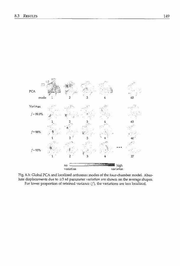
8.3 RESULTS

PCA

mode 1

Varimax

1

/""98% #

1

/=95%

1

2 3 4

)\

2 3 4 ,,

~

2 3 4'

2 3 4

no c======··ijJ+:,lill>Z'lliJ3i:ll<!lllilliiiliiilill J:Ugh variation variation

63

63

40

27

Fig. 8.3: Global PCA and localized orthomax modes of the four-chamber model. Abso­lute displacements due to :::i::::3 sd parameter variation are shown on the average shapes.

For lower proportion of retained variance (f), the variations are less localized.

149

150 WALL MOTION CLASSIFICATION

Table 8.2: Classification accuracy in multiple segments versus the number of PCA and varimax shape parameters used, for combinations of segments. N denotes the number of segments which were combined. The percentage of normal motion of all data sets

is also listed.

Classification accuracy #Para-View Segment (N) normal TRNL-1-0 TST meters

PCA/=99.9%

4C+2C All (9) 25.6% 89.2% 70.3% 11 4C Total4C (5) 22.5% 87.7% 78.1% 13 2C Total2C (5) 6.2% 100% 96.9% 21 4C Septal (2) 29.5% 100% 67.2% 28 4C Lateral (2) 49.6% 81.5% 70.3% 10 2C Anterior (2) 61.2% 93.8% 73.4% 11 2C Inferior (2) 30.2% 93.8% 75.0% 14

2-segment combinations: mean 42.6% 92.3% 71.5% 15.8 sd 15.5% 7.8% 3.5% 8.3

Varimax f = 99.9%

4C+2C All (9) 100% 70.9% 47 4C Total4C (5) 96.9% 81.3% 18 2C Tota!2C (5) 100% 96.9% 35 4C Septal (2) 92.3% 64.1% 24 4C Lateral (2) 90.8% 70.3% 8 2C Anterior (2) 93.8% 75.0% 9 2C Inferior (2) 98.5% 76.6% 14

2-segment combinations: mean 93.9% 71.5% 13.8 sd 3.3% 5.6% 7.3

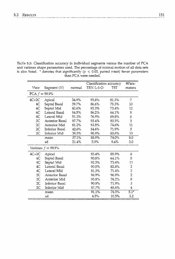
8.3 REsmrs

Table S.3: Classification accuracy in individual segments versus the number of PCA and varimax shape parameters used. The percentage of normal motion of all data sets is also listed. * denotes that significantly (p < 0.05, paired t-test) fewer parameters

than PCA were needed.

Classification accuracy #Para-View Segment (N) normal TRN L-1-0 TST meters

PCA/=99.9%

4C+2C Apical 34.9% 93.8% 81.3% 7 4C Septal Basal 59.7% 86.6% 70.3% 10 4C Septal Mid 42.6% 92.3% 73.4% 12 4C Lateral Basal 84.5% 86.2% 64.1% 8 4C Lateral Mid 51.2% 76.9% 69.8% 6 2C Anterior Basal 97.7°/o 95.4°/o 95.3% 3 2C Anterior Mid 61.2% 93.8% 74.6% 11 2C Inferior Basal 42.6% 84.6% 71.9% 5 zc Inferior Mid 39.5% 90.8% 65.6% 10

mean 57.1% 88.9% 74.0% 8.0 sd 21.4% 5.9% 9.4% 3.0

Varimax f = 99.9%

4C+2C Apical 95.4% 85.9% 6 4C Septal Basal 90.8% 64.1% 5 4C Septal Mid 92.3% 73.4% 11 4C Lateral Basal 90.8% 82.8% 2 4C Lateral Mid 81.5% 71.4% 2 2C Anterior Basal 96.9% 96.9% 2 2C Anterior Mid 93.8% 76.2% 9 2C Inferior Basal 90.8% 71.9% 5 2C Inferior Mid 87.7% 65.6% 4

mean 91.1% 76.5% 5.1'" sd 4.5% 10.5% 3.2

151

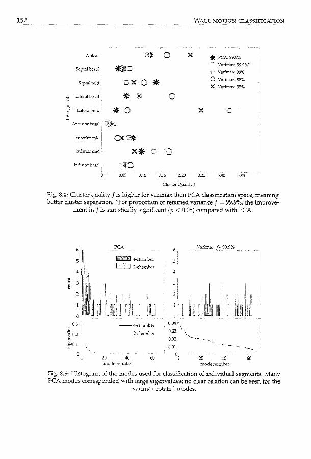
152

Apical

Septal bJs.Jl ~=

Septal mid =x c LaterJ! basal * v E ~

Lateral mid * ;0 ~

:; Anterior bosal ~~~

Anterior mid

Inferior mid

Inferior bJsal :~0 0.05

3~ ()

0 * :·~· 0

0.10 0.15 0.20

X

WALL MOTION CLASSIFICATION

X

0.25

* PCA99.9% Vorirnax, 99.9% ..

= Varimax, 99%

0 Vorimax, 98%

X V;:uimax, 95%

0.30 0.35

Ouster Quo.Jity J

Fig. 8.4: Cluster quality J is higher for varimax than PCA classification space, meaning better cluster separation. *For proportion of retained variance f = 99.9%, the improve­

ment in J is statistically significant (p < 0.05) compared with PCA.

6

5

4

~ 3 8 2

0

0.3 i, v 0

"3 02 2 0 -~0.1 0

0 1

.. 20

PCA

Wli@S±\VM 4-chombcr

~ 2-cho.mbcr

:[r 11r,r, ,, ~t:· _:I

--4-ch.amber

2-cl:umber

40 60 mode number

6' Varirrtax_ f = 99.9%

5

4

3'

2! ,,

0

··, ~ ~~ i!,

0.04 '!\ 0.03i~ 0.02 i ·--.........__

I

I ,,. ;; ·:. i

l''l:l'irlli·' L1 1

0.01 ··- ~- ···----...__

o, 20 40 60 mode number

fig. 8.5: Histogram of the modes used for classification of individual segments. Many PCA modes corresponded with large eigenvalues; no clear relation can be seen for the

varimax rotated modes.

8.4 DISCUSSION 153

Discussion 8.4

Localized shape models of the left ventricle, generated using orthomax rotations, were more effective in classifying local wall motion. Significantly fewer parame­ters were needed for classifying segmental wall motion in 2D echocardiographic sequences, while preserving classification accuracy.

Orthomax criteria 8.4.1

Similar results were obtained for the quartimax, factor parsimony, and varimax criteria, probably because the reparameterizations were restricted by the allowable variations in the training set, rather than the actual criterion. In fact, similar modes can be found for each criterion. This suggests that the criterion used has only a minor influence on the localization. Varimax is a commonly used criterion, and often implemented in statistical packages, making it desirable for use.

Proportion of retained variance 8.4.2

Best results were obtained using all PCA modes before the orthomax rotation. More modes in the original PCA model means more degrees of freedom for the rotation. As a result, the rotated basis is sparser, so the variations are more lo­calized (Fig. 8.3). Thus, fewer parameters needed to be combined to classify an individual segment.

Segmental classification 8.4.3

For classification of five or more segments, more orthomax parameters are used than PCA parameters. This is as expected, because more localized modes must be combined to explain global variations. However, when classifying combina­tions of two segments, a slight decrease in the number of parameters can already be observed. Localization of model modes results in much more subtle motion patterns, which are more meaningful for local wall motion classification.

It is important to keep in mind that the orthomax method automatically gener­ates sparse representations, given the variations in the training set. The relatively large improvement in the number of used modes in the lateral region may be due to the combination of the orthomax rotation and these training variations, which by chance produced a sparser parameter representation in those segments. The same holds for segments in which the improvement was smaller (e.g. the septal mid segment).

The fact that the used orthomax modes did not correlate with variance sug­gests that better methods may be needed to categorize these modes (Fig. 8.5). Recently, Suinesiaputra eta!. [2004] suggested that modes may be ordered locally, which is of particular interest for local classification. This is a subject of further investigation.

154 WALL MOTION CLASSIFICATION

8.'1.4 Visual wall motion scoring and alternatives

The absence of a true gold standard for diagnosing cardiac disease is a limitation of this study. Stress echo is noted for its variability in visual scoring [Hoffmann et al., 1996]. Regrettably, this variability could not be determined for this data set because the scoring was performed by consensus.

More objective measures as gold standard would be helpful in evaluating the orthomax method. For example, quantitative deformation parameters, derived from tissue Doppler imaging [Armstrong et al., 2000], or strain/strain-rate of speckle tracking techniques [Helle-Valle et al., 2005], can be used. A step further would be to relate quantitative coronary angiography data with the orthomax shape modes. This is more challenging, because shape modes are related to the myocardial contractility, and not directly to coronary artery disease.

8.4\.5 Limitations of study setup

Although the goal of this study is to show the compactness of the orthomax rep­resentation, it will be interesting to see if the classification accuracy actually im­proves with the sparse approach. To draw solid conclusions, many more patients need to be analyzed. Also, the choice of classifier may impact the performance. The cluster quality J (Fig. 8.4) revealed that there is still a reasonable amount of overlap of the classes, suggesting that better classification may be achieved with a nonlinear discriminant function. More advanced feature selection methods and nonlinear classifiers, such as support vector machines, may lead to better classifi­cation accuracy.

The proposed method could be directly applied to Dobutamine stress images, rather than the rest images alone. Also, the parasternal short-axis and long-axis images were not available for modeling. Combined models for rest and stress, or models of differences between these two, are also an option to explore [Suinesia­putra eta!., 2005]. Finally, with the recent interest in 3D stress echocardiography [Aggeli et al., 2007; Pulerwitz et al., 2006], orthomax rotations should be useful there as well.

8.4.6 Orthomax extensions and alternatives

Although orthomax is particularly interesting in terms of computational effi­ciency, it would be interesting to compare the proposed orthomax method with other localization methods, such as tndependent component analysis [l}zfuncu et al., 2003] and sparse PCA methods [Sjostrand et al., 2006; Zou et al., 2004]. Alter­natives which make use of the intensity patterns, instead of shapes, might also be interesting [Frouin et al., 2004].

Although not explored here, sparse texture models can be constructed in a very similar manner [Stegmann et al., 2006]. The direct cardiac application would be to examine local myocardial thickening, which might also be a predictor of coronary disease. Such texture models might be more suitable for image modal­ities such as magnetic resonance imaging rather than echocardiography, which

8.5 CoNCLUSIONs 155

suffers from speckle noise.

Conclusions 8.5

In this chapter we showed that classification of local left ventricular wall motion is feasible using local shape models, obtained with orthomax rotations. Due to the localization of shape variation, the classification needs fewer parameters to obtain similar accuracy with respect to normal global models.

Since pathologies are typically spatially localized, we anticipate many medical applications where sparse representations are preferred to the conventional PCA approach. The orthomax criterion is shown to be suitable for building these sparse representations with relative ease. Researchers interested in local modeling are encouraged to explore the technique and use it for their own application.

Acknowledgments

We thank 0. Kamp and F. Nijland for providing the patient data. M. Sonka and M. B. Stegmann are gratefully acknowledged for the useful discussions.

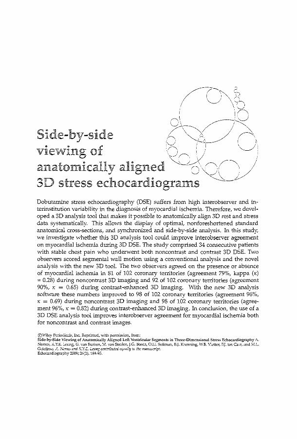
/7--~s / ~ \~~'

.... ~ . .. ~·~.. .:·v

Side-by-side 00--~\ viewt in~ o£

11 1. d \2nj/ ~' ~'"---<

ana omtca y a tgne - 8'\. __ / V 3D stress echocardiograms ~-~ Dobutamine stress echocardiography (DSE) suffers from high interobserver and in­terinstitution variability in the diagnosis of myocardial ischemia. Therefore, we devel­oped a 3D analysis tool that makes it possible to anatomically align 3D rest and stress data systematically. This allows the display of optimal, nonforeshortened standard anatomical cross-sections, and synchronized and side-by-side analysis. In this study, we IDvestigate whether this 3D analysis tool could improve interobserver agreement on myocardial ischemia during 3D DSE. The study comprised 34 consecutive patients with stable chest pain who undervvent both noncontrast and contrast 3D DSE. Two observers scored segmental wall motion using a conventional analysis and the novel analysis vvith the new 3D tool. The tvvo observers agreed on the presence or absence of myocardial ischemia in 81 of 102 coronary territories (agreement 79%, kappa (x) = 0.28) during noncontrast 3D imaging and 92 of 102 coronary territories (agreement 90%, K = 0.65) during contrast-enhanced 3D imaging. With the new 3D analysis software these numbers improved to 98 of 102 coronary territories (agreement 96%, K = 0.69) during noncontrast 3D imaging and 98 of 102 coronary territories (agree­ment 96%, K = 0.82) during contrast-enhanced 3D imaging. In conclusion, the use of a 3D DSE analysis tool improves interobserver agreement for myocardial ischemia both for noncontrast and contrast images.

©1A'iley PcriodicJ.L<:, Inc. Reprinted, with permission, from: Side-by-Side Viewing of Anatomically Alignt:d Ldt Vt:ntrkula:r St:gments in Three-Dimt:nsional Strl'Ss Echoca:rdiography A :Nemes, KY.E. Ll'ung.. G. mn Burken, :vr. wm Str.:llen,J.G. Bosch, O.I.I. Sol.im.m, B.J. Krenning, W.B. Vlettcr, F.J. to:>n C;:~tc, ;md M.L. Gdl'ijn..-<c. A. Nemes and K.Y.E. L..:ung contn"butcd cqWJlly to tlu manuscn"pt. EchocJrdiogr;:~phy 2009; 26{2), 189-95.

158 SIDE-BY-SIDE VIEWING

9.1 Introduction

Dobutamine stress echocardiography (DSE) is an accepted tool for the diagnosis of coronary artery disease (CAD) [Geleijnse et al., 1997]. The interpretation of the echocardiographic images, however, is critically dependent on the experience of the observer. Unfortunately, a high interobserver and interinstitution ariability in the diagnosis of myocardial ischemia is present [Hoffmann et al., 1996; Picano et al., 1991]. Recently, 3D echocardiography has become an option for DSE analysis [Aggeli et al., 2007; Matsumura et al., 2005; Nemes et al., 2007a,b; Pulerwitz et al., 2006; Takeuchi et al., 2006; Takuma et al., 2000]. 3D echo provides the possibil­ity to eliminate differences in cross-sections between rest and stress stages, since these cross-sections can be selected retrospectively. Unfortunately, there is cur­rently no software that enables clinicians to analyze 3D images at different stress stages side-by-side. Moreover, the comparison of nonforeshortened and identical cross-sections during rest and stress, one of the potential benefits of 3D imaging, depends on manual selection of these images, which is a complex 3D task. There­fore, we developed a specialized tool for 3D stress echo analysis. With this tool it is possible to anatomically align 3D rest and stress data systematically, to generate optimal, nonforeshortened standard anatomical cross-sections and to analyze the images synchronized and side-by-side. The specific objective of this investigation was to evaluate whether this 3D tool could improve interobserver agreement on myocardial ischemia during 3D DSE.

9.2 Patients and methods

9.2.1 Patient population

The study comprised 34 patients (22 men, mean age 57 ± 13 years) in sinus rhythm with chest pain referred for stress testing. These patients were previously included in a study by our group in which the usefulness of ultrasound contrast in 3D DSE was assessed [Nemes et al., 2007b]. The institutional review board approved the study and all patients gave informed consent.

9.2.2 Dobutamine-atropine stress protocol

Dobutamine was administered through a peripheral vein by 3-min stages of 10, 20, 30, and 40 l'g/kg/min, respectively. The infusion was stopped when 85% of age-predicted maximum heart rate was reached. Otherwise, Dobutamine infusion was continued and supplemented by 0.25 mg doses of atropine (to a maximal dose of 1 mg). The stress test was terminated when severe angina, shortness of breath, symptomatic decrease in systolic blood pressure (>40 rnmHg), arterial hypertension (>240/120 rnmHg), severe arrhythmias or other serious adverse

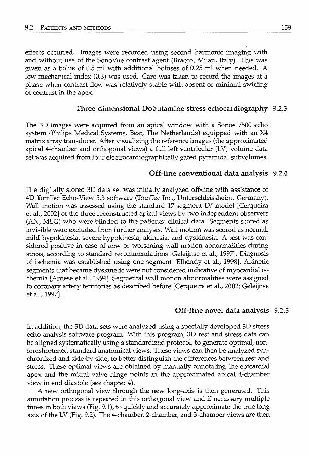
9.2 PATIENTS AND METHODS

effects occurred. Images were recorded using second harmonic imaging with and without use of the SonoVue contrast agent (Bracco, Milan, Italy). This was given as a bolus of 0.5 ml with additional boluses of 0.25 ml when needed. A low mechanical index (0.3) was used. Care was taken to record the images at a phase when contrast flow was relatively stable with absent or minimal swirling of contrast in the apex.

159

Three-dimensional Dobutamine stress echocardiography 9.2.3

The 30 images were acquired from an apical window with a Sonos 7500 echo system (Philips Medical Systems, Best, The Netherlands) equipped with an X4 matrix array transducer. After visualizing the reference images (the approximated apical 4-chamber and orthogonal views) a full left ventricular (LV) volume data set was acquired from four electrocardiographically gated pyramidal subvolurnes.

Off-line conventional data analysis 9.2.4

The digitally stored 30 data set was initially analyzed off-line with assistance of 40 TomTec Echo-View 5.3 software (TomTec Inc., Unterschleissheim, Germany). Wall motion was assessed using the standard 17-segment LV model [Cerqueira eta!., 2002] of the three reconstructed apical views by two independent observers (AN, MLG) who were blinded to the patients' clinical data. Segments scored as invisible were excluded from further analysis. Wall motion was scored as normal, mild hypokinesia, severe hypokinesia, akinesia, and dyskinesia. A test was con­sidered positive in case of new or worsening wall motion abnormalities during stress, according to standard recommendations [Geleijnse et a!., 1997]. Diagnosis of ischemia was established using one segment [Elhendy et a!., 1998]. Akinetic segments that became dyskinetic were not considered indicative of myocardial is­chemia [Arnese et al., 1994]. Segmental wall motion abnormalities were assigned to coronary artery territories as described before [Cerqueira eta!., 2002; Geleijnse eta!., 1997].

Off-line novel data analysis 9.2.5

In addition, the 30 data sets were analyzed using a specially developed 3D stress echo analysis software program. With this program, 30 rest and stress data can be aligned systematically using a standardized protocol. to generate optimal, non­foreshortened standard anatomical views. These views can then be analyzed syn­chronized and side-by-side, to better distinguish the differences between rest and stress. These optimal views are obtained by manually annotating the epicardial apex and the mitral valve hinge points in the approximated apical 4-chamber view in end-diastole (see chapter 4).

A new orthogonal view through the new long-axis is then generated. This annotation process is repeated in this orthogonal view and if necessary multiple times in both views (Fig. 9.1), to quickly and accurately approximate the true long axis of the LV (Fig. 9.2). The 4-chamber, 2-chamber, and 3-chamber views are then

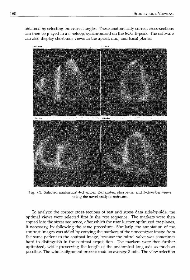
160 SIDE-BY-SIDE VIEWING

obtained by selecting the correct angles. These anatomically correct cross-sections can then be played in a cineloop, synchronized on the ECG R-peak. The software can also display short-axis views in the apical, mid, and basal planes.

Fig. 9.1: Selected anatomical 4-chamber, 2-chamber, short-axis, and 3-chamber views using the novel analysis software.

To analyze the correct cross-sections of rest and stress data side-by-side, the optimal views were selected first in the rest sequence. The markers were then copied into the stress sequence, after which the user further optimized the planes, if necessary, by following the same procedure. Similarly, the annotation of the contrast images was aided by copying the markers of the noncontrast image from the same patient to the contrast image, because the mitral valve was sometimes hard to distinguish in the contrast acquisition. The markers were then further optimized, while preserving the length of the anatomical long-axis as much as possible. The whole aligrunent process took on average 3 min. The view selection

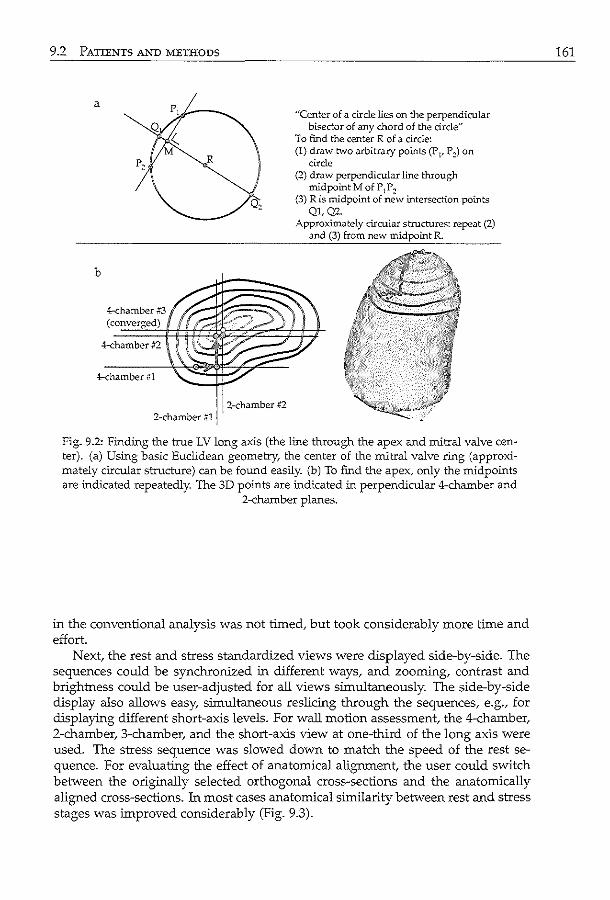
9.2 PATIENTS A>-'D METHODS

a

b

4-chamber #3 (converged)

4-chamber #2

4-chamber #1

2-chamber #1 2-chamber #2

"Center of a circle lies on the perpendicular bisector of any chord of the circle"

To find the center R of a circle: (I) draw two arbitrary points (Pp P ~)on

circle (2) draw perpendicular line throug-h

midpoint M of P1Pz (3) R is midpoint of new intersection points

QJ,Q2. Approximately circular structures: repeat (2)

and (3) from new midpoint R.

Fig. 9.2: Findillg the true LV long axis (the line through the apex and mitral valve cen­ter). (a) Using basic Euclidean geometry, the center of the mitral valve ring (approxi­mately circular structure) can be found easily. (b) To find the apex, only the midpoints are indicated repeatedly. The 3D points are indicated in perpendicular 4-chamber and

2-chamber planes.

in the conventional analysis was not timed, but took considerably more time and effort.

Next, the rest and stress standardized views were displayed side-by-side. The sequences could be synchronized in different ways, and zooming, contrast and brightness could be user-adjusted for all views simultaneously. The side-by-side display also allows easy, simultaneous reslicing through the sequences, e.g., for displaying different short-axis levels. For wall motion assessment, the 4-chamber, 2-chamber, 3-chamber, and the short-axis view at one-third of the long axis were used. The stress sequence was slowed down to match the speed of the rest se­quence. For evaluating the effect of anatomical alignment, the user could switch between the originally selected orthogonal cross-sections and the anatomically aligned cross-sections. 1n most cases anatomical similarity between rest and stress stages was improved considerably (Fig. 9.3).

161

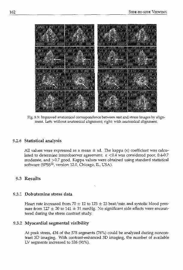
162 SIDE-BY-SIDE VIEWING

Fig. 9.3: Improved anatomical correspondence be-t.vveen rest and stress images by align­ment. Left: vvi.thout anatomical alignment; right: 'With anatomical alignment.

9.2.6 Statistical analysis

All values were expressed as a mean ± sd. The kappa (K) coefficient was calcu­lated to determine interobserver agreement. " <0.4 was considered poor, 0.4-0.7 moderate, and >0.7 good. Kappa values were obtained using standard statistical software (SPSS®, version 12.0, Chicago, IL, USA).

9.3 Results

9.3.1 Dobutamine stress data

Heart rate increased from 70 ± 12 to 123 ± 23 beat/min and systolic blood pres­sure from 127 ± 20 to 141 ± 31 mmHg. No significant side effects were encoun­tered during the stress contrast study.

9.3.2 Myocardial segmental visibility

At peak stress, 434 of the 578 segments (76%) could be analyzed during noncon­trast 3D imaging. With contrast-enhanced 3D imaging, the number of available LV segments increased to 526 (91 %).

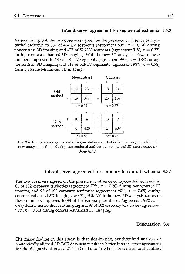
9.4 DISCUSSION 163

Interobserver agreement for segmental ischemia 9.3.3

As seen in Fig. 9.4, the two observers agreed on the presence or absence of myo­cardial ischemia in 387 of 434 LV segments (agreement 89%, K = 0.24) during noncontrast 3D imaging and 477 of 526 LV segments (agreement 91%, K = 0.37) during contrast-enhanced 3D imaging. With the new 3D analysis software these numbers improved to 430 of 434 LV segments (agreement 99%, K = 0.83) during noncontrast 3D imaging and 516 of 526 LV segments (agreement 98%, K = 0.78) during contrast-enhanced 3D imaging.

N oncontrast Contrast + +

+ 10 28 + 18 24 Old

method 19 377 25 459

K=0.24 K-0.37

+ +

+~ +~ New method

- 0 420 - 1 497

K= 0.83 K=0.78

Fig. 9.4: Interobserver agreement of segmental myocardial ischemia us:ing the old and new analysis methods during conventional and contrast-enhanced 3D stress echocar­

diography.

Interobserver agreement for coronary territorial ischemia 9.3.4

The two observers agreed on the presence or absence of myocardial ischemia in 81 of 102 coronary territories (agreement 79%, K = 0.28) during noncontrast 3D imaging and 92 of 102 coronary territories (agreement 90%, K = 0.65) during contrast-enhanced 3D imaging, see Fig. 9.5. With the new 3D analysis software these numbers improved to 98 of 102 coronary territories (agreement 96%, K =

0.69) during noncontrast 3D imaging and 98 of 102 coronary territories (agreement 96%, K = 0.82) during contrast-enhanced 3D imaging.

Discussion 9.4

The major finding in this study is that side-by-side, synchronized analysis of anatomically aligned 3D DSE data sets results in better interobserver agreement for the diagnosis of myocardial ischemia, both when noncontrast and contrast

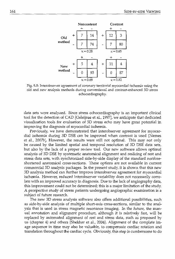
164

Old method

New method

Noncontrast +

·1 :1:: I x=0.28

+

•tffi_j x= 0.69

Contrast +

SIDE-BY-SIDE VIEWING

•t-ffij x=0.65

+

•tffij x=0.82

Fig. 9.5: Interobserver agreement of coronary territorial myocardial ischemia using the old and new analysis methods during conventional and contrast-enhanced 3D stress

echocardiography.

data sets were analyzed. Since stress echocardiography is an important clinical tool for the detection of CAD [Geleijnse eta!., 1997], we anticipate that dedicated visualization tools for evaluation of 3D stress echo may have great potential in improving the diagnosis of myocardial ischemia.

Previously, we have demonstrated that interobserver agreement for myocar­dial ischemia during 3D DSE can be improved when contrast is used [Nemes et al., 2007b ]. However, the results were still not optimal. This may not only be caused by the limited spatial and temporal resolution of 3D DSE data sets, but also by the lack of a proper review tool. Our new software allows optimal analysis of 3D DSE by systematic anatomical alignment and reslicing of rest and stress data sets, with synchronized side-by-side display of the standard nonfore­shortened anatomical cross-sections. These options are not available in current commercial 3D analysis packages. In the present study, it is shown that this new 3D analysis method can further improve interobserver agreement for myocardial ischemia. However, reduced interobserver variability does not necessarily corre­late with an improved accuracy in diagnosis. Due to the lack of angiography data, this improvement could not be determined; this is a major limitation of the study. A prospective study of stress patients undergoing angiographic examination is a subject of future research.

The new 3D stress analysis software also offers additional possibilities, such as side-by-side analysis of multiple short-axis cross-sections, similar to the anal­ysis that is used in stress magnetic resonance imaging. In the future, the man­ual annotation and alignment procedure, although it is relatively fast, will be replaced by automated alignment of rest and stress data, such as proposed by us (chapter 4) and others [Shekhar et a!., 2004]. Alignment of the complete im­age sequence in time may also be valuable, to compensate cardiac rotation and translation throughout the cardiac cycle. Obviously, this step is cumbersome to do

9.4 DISCUSSION

manually and should therefore be automated [Shekhar eta!., 2004]. The alignment can also serve as a solid basis for automated segmentation of 3D stress echo data and automatic quantification of LV wall motion [Bosch et al., 2005; van Stralen et a!., 2005a; Zagrodsky et a!., 2005].

An intriguing finding in this study is that the use of systematically aligned anatomical views resulted in a higher number of LV segments that are scored as nonischemic. This may suggest a higher specificity (but also a reduced sensitiv­ity) for the diagnosis of CAD. Observers are used to imperfectly aligned, slightly foreshortened views. In such views, wall thickness and wall motion is overesti­mated, and differences in alignment and foreshortening in rest and stress may be falsely interpreted as a change in wall thickening and motion. If the optimal non­foreshortened cross-sections are visualized, thickening and motion will be more consistent between rest and stress, but abnormalities may be subtler to detect (and may need some retraining of the eye). We anticipate that this will result in less false positive studies, and thus a better specificity for the diagnosis of CAD. To study the true effects of our new analysis software on the diagnostic value of 3D DSE, a larger cohort of patients undergoing diagnostic coronary angiography should be studied prospectively.

165

Discussion and conclusions

168 DISCUSSION AND CONCLUSIONS

10.1 Research goals

Cardiovascular diseases are one of the major causes in the Western world. Im­provement of diagnostic techniques is therefore of great clinical importance. A widely-applied diagnostic method for assessing myocardial dysfunction and un­derlying coronary disease is stress echocardiography. Wall motion of the left ventricle is visualized with echocardiography (ultrasound imaging) at rest and at different levels of stress (elevated to maximal workload for the cardiac mus­cle). Traditionally, the wall motion is analyzed visually by 'eyeballing' cross­sectional anatomical views, acquired using two-dimensional (2D) imaging tech­niques. Hence, traditional2D stress echo suffers from differences in the visualized cross-sections, within the same patient as well as between different patients. Also, 2D stress echo is hampered by observer variabilities in the visual analysis.

Recently, three-dimensional (3D) ultrasound imaging has been proposed for stress echocardiography. 3D imaging may offer a better definition of anatomical views after the image acquisition, and better possibilities for objective quantifica­tion of 3D wall motion. Quantification in 3D ultrasound imaging is not an easy task. Suboptimal spatial and temporal image resolution results in inferior image quality; the various ultrasound specific imaging artifacts hamper the imaging of parts of the left ventricle; and the wealth of 3D data requires dedicated automated methods to avoid tedious manual, thus subjective, analysis. In this thesis, such automated methods are presented, for objective and quantitative analysis of 3D stress echo.

To enable automated analysis, methods have been developed for o detection of anatomical markers and automated view selection (chapters 2-4),

for improving visualization and for initialization of other automated methods, o segmentation of left ventricular endocardial borders throughout the cardiac

cycle (chapters 5-7), for deriving left ventricular motion parameters, and o classification of these parameters into normal and pathological motion (chap-

ter 8). In addition, we present a clinical evaluation of a dedicated 3D stress echo software package, which has been developed in the course of this research project (chapter 9). This package is intended as a tool for facilitating analysis of 3D stress echo.

10.2 Summary of contributions

10.2.1 Initialization

For anatomical marker detection and automated view selection, we chose to ex­plore initialization methods based on model-to-image registration, feature detec­tion via the Hough transform, and image-to-image registration.

For initial landmark detection, a model-to-image registration approach was

10.2 SUMMARY OF CONTRIBUTIONS

investigated, in which a statistical appearance model of the left ventricle was matched to an image to find the anatomical landmarks (see chapter 2). To make the model more concise, only a sparse set of landmarks on commonly used anatomical views (four-chamber, two-chamber, and short-axis) were modeled. By matching the pose and model parameters in a registration framework, no cum­bersome training of the optimizer was needed (unlike the traditional active ap­pearance model algorithm). The evaluation, albeit on a limited number of data sets, showed that the normalized cross-correlation metric gave better results than the sum-of-square differences, sum-of-absolute differences, and normalized mu­tual information metrics. The increase in the number of model parameters (from 67% to 96% variance coverage) resulted only in a slight improvement ( < lmm point-to-point) of the matching results. This confirmed that the matching of the pose and the principal modes were more important for initial alignment. The re­sulting alignment had an error of approximately Smm, which should be adequate for initializing the active appearance model with the Jacobian tuning algorithm as described in chapter 5 (see Fig. 5.4).

In chapter 3, a method was presented for finding the long-axis and mitral valve plane of the left ventricle in the whole cardiac cycle. As opposed to the model-based registration method in chapter 2, the methods used are data-driven. The long-axis in each individual 3D image was found by applying the Hough transform for circles in approximate short-axis cross-sections. The resulting cen­ters were spatially and temporally regularized using multidimensional dynamic progranmting for a more robust and time continuous result. The mitral valve plane was found also by using dynamic progranmting; the endocardial borders were detected in spherically interpolated images and the mitral valve was found via backprojection in the cartesian domain. The method showed robust results in terms of angle and distance errors in data of 25 patients. The errors were comparable to interobserver variabilities and the algorithm had low computation costs.

Given annotated landmarks in a rest image, the landmarks in the correspond­ing stress image were obtained using image-to-image registration (see chapter 4). Instead of using the whole 3D image, only the common anatomical views were used to calculate the image metric. Qualitative and quantitative evaluation in 20 end-diastolic and 20 end-systolic data sets showed an improvement in alignment after registration. Again, the normalized cross-correlation metric proved to give good results, close to the interobserver variability. It was shown that a more ro­bust landmark detection was obtained using this sparse distribution of anatomical views, rather than using the whole 3D image. By using a registration approach, we exploited the fact that intra patient variability is smaller than interpatient vari­ability. This is especially important, given that the quality of stress images is generally lower than that of the rest images (see also Nemes et al. [2007b]).

169

Segmentation :w.2.2

For detecting the endocardial border of the left ventricle, we proposed segmenta­tion methods based on active appearance models and optical flow tracking. The

170 DISCUSSION AND CONCLUSIONS

latter was further improved by assigning lower probabilistic weights to image pixels corresponding with stationary artifacts.

The active appearance model (AAM) technique was applied for detecting the left ventricular contours in a single 3D image in chapter 5. This method matched a statistical model of shape and texture to an image via regression tech­niques, which required training of the regression matrix. The traditional matching method was compared with a new 'Jacobian tuning' method, which updated the regression matrix during matching instead of using a fixed matrix. Better accu­racy and a larger capture range were obtained using the Jacobian tuning method in 54 patients. The larger capture range has important repercussions in applying the AAM to ultrasound images, given the variability of left ventricular appearance and the large amount of information due to 3D modeling.

Segmentation in the whole cardiac cycle was posed as a tracking problem in chapter 6. The contour in an end-diastolic 3D image is propagated throughout the image sequence using spatial transforms, calculated with optical flow. A sta­tistical model of cardiac motion was embedded in the optical flow calculation, for a time-continuous and physically plausible segmentation, even at sites where the myocardial wall was obscured. Good tracking results were obtained in 53 non­contrast images and 27 contrast images, comparing well with results reported in literature. The combination of the proposed motion-guided method with the ba­sic, purely data-driven optical flow method using gradient-based weights proved to be best for good quality images. For more challenging images, the motion­guided method provided still good results, whereas the basic method had more difficulties in tracking.

To further improve the tracking method, a probabilistic weight scheme was proposed in chapter 7 to improve the balance between the motion-guided and the basic tracking approaches. The idea was to rely on the basic tracking if the myocardial wall was clearly visible, and to use the motion-guided method in areas where the myocardial wall was obscured by artifacts such as near-field clut­ter and shadowing. This balance was determined by calculating weights using temporal image intensity information. The evaluation on 35 noncontrast image sequences showed a further improvement in tracking accuracy, compared with the gradient-based weights proposed in chapter 6. This shows that the detection of such artifacts, which are often seen in clinical quality images, are beneficial in terms of segmentation accuracy.

10.2.3 Classification

In chapter 8, the automated classification of segmental wall motion abnormali­ties was investigated. A model of the left ventricular shape in multiple cardiac phases was used to generate simple parameters which characterized wall mo­tion. The orthomax rotation was applied to generate an even more concise model for classifying segmental wall motion. The resulting classification of 2D+time echocardiograms was shown to have similar accuracy using fewer parameters in a better-defined classification space. An additional bonus is that the orthomax rotation is readily available in statistical analysis software, making it easy to use

10.3 DISCUSSION OF CO"-'TRIBUTIONS 171

in other applications.

Clinical application 10.2.4

The first clinical application of the 3D stress echo software was shown in chapter 9. The software allowed proper display of the stress echo images, with different stress stages side-by-side and (manually) anatomically aligned. Using this soft­ware, interobserver agreement was shown to drastically improve compared with traditional software (which did not feature side-by-side display nor systematic alignment), in the analysis of 34 stress noncontrast and contrast data sets. This shows that the use of dedicated software is of importance in the analysis 3D stress echo.

Discussion of contributions 10.3

The goal of this thesis is to present methods which contribute toward the auto­mated analysis of 3D stress echo. In the following, we will discuss the suitability and applicability of these methods in the general clinical setting, keeping in mind the requirements that the methods should enable fast, robust and ac=ate analy­sis.

Registration 10.3.1

In chapters 2 and 4, we proposed methods using the registration paradigm. Since registration is an optimization process in which the image metric is evaluated during each iteration, the method is traditionally slow, and increasingly so with the number of parameters. With improvements like limiting the metric calcula­tion to specific image areas, great gain in computation speed can be obtained. This is important for initialization purposes, since the initialization is not the fi­nal step in the analysis. Since the computation times reported were based on an implementation in a prototype environment (10-20 minutes in MATLAB), they may give an unrealistically pessimistic view of the methods' speed. With further optimizations and improvements in implementation (e.g. using the graphics card for image interpolation), registration time can probably be brought down to a few seconds (provided that the number of parameters to optimize is limited).

The ac=acy of the proposed registration methods is probably adequate for initializing contour detection method purposes. While registration itself has been shown to be able to provide subpixel accuracy, the errors reported seem rather large. This may partly be a result of the difficulties in establishing ground truth via manual annotation. Also, compared with modalities like CT and MR, ultra­sound suffers more from artifacts and speckle noise, making both manual anno­tation and automated processing more difficult.

The registration paradigm relies heavily on the fact that the images to be regis­tered must be similar. For the model-to-image registration (chapter 2), the robust-

172 DISCUSSION AND CONCLUSIONS

ness depends on the ability of the model to approximate an image outside the training set (also known as model generalization). To improve this model gen­eralization, we have chosen to only model the appearance on sparse anatomical views. For the image-to-image registration, the template should be similar to the target image. In our case, this was achieved by matching the rest and stress im­ages of the same patient, instead of using a model-to-image registration approach for the stress images.

10.3.2 Model-based analysis

Statistical models were included in the methods of chapters 2, 5, 6, 7, and 8. In chapters 2 and 5, shape and texture models were used to describe the variations in left ventricular appearance. Chapters 6 and 7 described models representing frame-to-frame affine cardiac motion. In chapter 8, a multiphase shape model was used for classification purposes.

The AAM technique has the advantage of providing faster parameter opti­mization (chapter 5) than registration (chapter 2), especially when many param­eters need to be optimized. The AAM achieves this by training the optimizer via regression techniques: the model is perturbed with chosen parameters and the differences between the model and training images are stored in a regression matrix. In the matching stage, the difference between the current estimation of the model and the testing image, together with the regression matrix, are used to calculate a linear update of the model parameters. Although the regression training stage is computationally demanding (a few hours), the matching stage is very fast (less than a minute).

The robustness and accuracy of the AAM method hinges on model gener­alization. For the current appearance model built using 54 samples, the shape model could achieve approximately 95% generalization in a leave-one-out sit­uation, whereas the texture model could only achieve 65% generalization [van Stralen et al., 2007]. This difference could be attributed to the fact that the shape model represents 2700 input (coordinate) values, whereas the texture model de­scribes 22500 (intensity) values. Since the traditional AAM matching algorithm uses a fixed regression matrix, the limited texture generalization might explain the reduced accuracy for larger perturbations in chapter 5 (Fig. 5.3, 5.4). It is pos­sible that the Jacobian tuning method is able to extend the limitations of model generalization by adapting the regression matrix during matching, resulting in a larger capture range.

Model generalization can be improved in a number of ways. The training samples should be representative of the testing population, e.g. containing both normal and pathological data. The number of modeled values can be limited by finding other representations, such as using affine transforms instead of actual 3D points (explored in chapters 6 and 7) or by modeling only local behavior [Seghers et al., 2007]. To make models more concise, spatial (interpatient: chapter 5) and temporal (intrapatient: chapters 6 and 7) behaviors were modeled separately in this thesis. Finally, models can be improved using more training samples. Ways of artificially augmenting the number of training samples have been proposed

10.3 DISCUSSION OF CONTRIBUTIONS

recently [Koikkalainen eta!., 2008]. Another important issue is that of point correspondence. To build a good

statistical model, the modeled points should represent distinct, consistent land­marks. In chapter 5, the 3D point correspondence is established using the long­axis and 4-chamber orientation. In chapters 6 and 7, there was a lack of temporal anatomical point correspondence, due to the use of a fixed coordinate system based on the annotated landmarks in end-diastole. As a result, the model did not represent motion tangential to the contour, and this type of motion could not be recovered when matching the model to the image.

Furthermore, methods can be applied which improve the modeling itself. Tra­ditional principal component analysis (PCA), which is most often used for statis­tical modeling, implicitly assumes that the underlying data has a single Gaussian distribution. For more complex distributions, multiple Gaussian models [Coates and Taylor, 1999] and other nonlinear methods [Twining and Taylor, 2001] can be used. Robust statistical methods for building and matching can be applied to deal with outliers in statistical modeling. Common methods are based on M­estimation and random sampling techniques [Rogers and Graham, 2002] (see also section 7.1.2).

Principal component analysis yields models of which the eigenmodes are or­dered according to variance. As a result, the main modes represent global mo­tion. In chapter 8, an alternative representation was investigated, which rotates the modes such that they represent local variations. While the model still contains the same amount of variation, it is more concise in modeling local behavior. As a result, the number of modes needed to classify local wall motion can be reduced. Also, the classification space was better behaved, which may potentially lead to better classification accuracy. However, many more patients need to be analyzed to draw a solid conclusion.

173

Feature-based analysis :W.3.3

In this thesis, we also investigated methods which operate on low-level image features, such as the circular Hough transform (chapter 3), dynamic programming (chapter 3), optical flow (chapters 6 and 7), and probabilistic pixel-wise weight schemes (chapter 7).

The Hough transform is a well-established method for detecting parametric structures in low quality images. In chapter 3, the Hough transform has been successfully applied for robustly detecting circular structures, even in the pres­ence of severe artifacts such as shadowing. By estimating circle centers in a set of short-axis views, the long-axis can be reconstructed more reliably. Although the Hough transform is an n-dimensional teclmique, in this work, we have chosen to detect 2D circle centers instead of the 3D long-axis line to limit computation time. For that same reason, we chose not to explore the generalized Hough trans­form [Ballard, 1981]. The computation time can be reduced by using multiscale techniques.

In chapter 3, the dynamic programming technique is used to regularize the estimates of the long-axis and to detect the mitral valve plane. Dynamic pro-

174 DISCUSSION AND CONCLUSIONS

gramming is a robust and fast technique for finding an optimal path through a directed graph. This technique is also used for generating left ventricular contours as ground truth semi-automatically in chapters 6, 7, and 8. For segmentation, the graph was constructed by resampling the image perpendicular to an iritial estimate of the contour. In 3D, this technique, together with smart choices for cost-functions, proved to generate LV volumes which were comparable with MRI [van Stralen eta!., 2005b]. Since dynamic programming is a search through a dis­crete parameter space, the accuracy also depends on the resolution of the directed graph, i.e. the distance between neighboring nodes. Alternative methods which can search paths through a continuous parameter space are state estimation meth­ods such as Kalman filtering [Maybeck, 1979] and particle filtering [Arulampalam et a!., 2002].

The optical flow method was applied in chapter 6 for tracking the cardiac motion. Previously, this method was applied successfully for tracking small-scale speckle in 2D images. Since the optical flow is a differential method based on calculation of spatial and temporal gradients, both spatial and temporal resolution are defiritely an important issue. Currently, the temporal resolution in 2D is more favorable than in 3D imaging. Despite this limitation, we have shown that tracking larger scale structures (the myocardial wall) in 3D is feasible with optical flow. The tracking of speckle in 3D is a subject of continuing research.

The purely data-driven optical flow method was quite accurate in estimating motion at sites with good myocardial wall visibility. However, the method had more problems in obscured areas. We have shown that the combination of the model-guided approach and the data-driven method leads to more robust and accurate tracking results in chapters 6 and 7. Another issue with the traditional optical flow method is that errors can accumulate throughout the image sequence if the tracking is performed on a frame-to-frame basis, as is implemented in chap­ters 6 and 7. In the case of a cardiac sequence, a backtracking approach (tracking from the end of the sequence to the front), may further improve results.

In chapter 7, we investigated a pixel-wise probabilistic weight scheme for dis­tinguishing between cardiac wall which is clearly visible and which is obscured. The weights were calculated by investigating the image intensity throughout the cardiac cycle. These weights were shown to have a positive effect on the robust­ness and accuracy of the tracking. The online expectation-maximization frame­work for calculating the weights themselves allowed for a fast computation which can attain real-time performance. Since the weight calculation is based on a pixel­wise evaluation, explicit spatial information is missing: e.g. the probability of encountering near-field artifacts is much higher close to the transducer than in other parts of the images. Also, in apically acquired echocardiograms, generally more shadowing artifacts are found in the anterolateral region of the left ventricle. Such prior information can be encoded, for example using a supervised classifi­cation approach. In that case, ground truth data (e.g. obtained using phantom experiments or manually annotated images) would be necessary.

10.3 DISCUSSION OF CONTRIBUTIONS 175

Accuracy for stress echo 10.3.4

Since traditional stress echo is analyzed visually, few reports can be found on quantification of regional wall motion within the vast amount of clinical litera­ture. This may be attributed to difficulties in cardiac wall delineations and the choice of reference standard (see also section 10.5.2). However, there is extensive literature on global clinical parameters such as volume and ejection fraction. In the following, we will discuss the accuracy of the automated methods in relation to clinical applicability in distinguishing between normal and abnormal function.

Few reports can be found on registration and view initialization, since 3D ultrasound imaging is a relatively new technique and view selection is not a post­processing issue for 2D imaging. Recently, Lu et al. [2008] reported a long-axis detection error of 8.2 ± 6.2' in a large database of 326 3D end-diastolic images. Orderud et al. [2009] reported errors of 11.8 ± 8.SO. In chapter 3, an error of 5 to 6' was reported, comparing quite favorably (see Table 3.3, 3.4 and Fig. 3.8). However, the mitral valve location can still be improved upon (Lu et al. [2008]: 3.6 ± 3.1mm, Orderud et al. [2009]: 3.6 ± 1.8mm, vs. chapter 3: 5.6 ± 3.1mm). For rest-to-stress registration, only qualitative results have been reported [Shekhar et al., 2004].

Global volume errors are more commonly reported (see Table 7 2). Our signed (1.4 ± 6.7ml) and absolute (5.2 ± 4.5ml) errors (Table 7.1) compare well with those reported in literature (Table 7.2). In chapter 7, absolute ejection fraction errors of 3.9 ± 2.9% were reported in a mixed population of 35 normal and abnormal sub­jects. According to Lang et al. [2006a ], reference limits for ejection fraction (based on 2D measurements) are :2: 55% for normal, 45%-54% for mildly abnormal, 30%-44% for moderately abnormal, and < 30% for severely abnormal left ventricular function. Using commercially available software, Soliman et al. [2007] found in­traobserver variabilities of 6.6 ± 7.4% (53 patients) and interobserver variabilities of 7.1 ± 6.9% in ejection fraction. This suggests that the proposed tracking method may be able to distinguish between these global differences in function.

Point-to-surface errors have been investigated more extensively in technical papers. Table 6.5 lists segmentation errors in technical papers, ranging from 1.5 ± 0.3mm to 3.4 ± 1.2mm; the Jacobian tuning method of chapter 5 (2.8 ± 1.0mm) is within this range. As for tracking errors, surface errors of 1.19 ± 0.47mm were found (chapter 7), which is in the range of the spatial resolution of the images (1 x 1 x 0.7mm). The obtained accuracy should be sufficient to distinguish between akinesis ( < 2mm) and normal(> Smm) endocardial excursion, at least in a global sense; however, these standard values were determined rather arbitrarily from 2D echocardiograms (see also section 10.5.2).

Comparison with quantitative regional measures is more difficult, since re­ports in literature often use their own definitions and a common standard is cur­rently lacking. In general, regional measures can be derived using imaging tech­niques (MRl: tagging [Prince and McVeigh, 1992], phase/velocity encoding [Pan et al., 2005], echo: acoustic quantification/ color kinesis [Mor-Avi et al., 1997], tis­sue Doppler [Armstrong et al., 2000]) or image processing techniques. Of the lat­ter, most often used are intensity based methods [Frouin et al., 2004; Kachenoura

176 DISCUSSION AND CONCLUSIONS

et a!., 2009], contour based (either direct measures like excursion or volume, or derived measures like in chapter 8), or tracking based (via registration or block­matching/ optical flow), see also Garcia-Femandez et a!. [2003] for an overview. Numerous measures exist [Peilikka, 2005], such as velocity [Voigt et a!., 2004], re­gional volumes [Nesser eta!., 2007], fractional area/volume change [Fujino eta!., 2001], wall thickening [Karagiannis et a!., 2007], strain/ strain-rate [Ingul et a!., 2007], contraction delays [Jenkins et a!., 2009], and torsion in short-axis images [Notomi eta!., 2005].

Here, we compare our tracking method with endocardial excursion values found in literature. DeCara et a!. [2004] measured 2D endocardial excursions (from a fixed spatial reference point) of 0-25mm (average 6mm, Fig .5 ofDeCara et a!. [2004]) with manually drawn end-diastolic and end-systolic contours and with color kinesis in 24 patients (also mixed population). Corsi eta!. [2005] found, us­ing their level-set contour detection method, that the regional shortening fraction (ED to ES motion divided by ED radial dimension) agreed with expert interpreta­tion of normality in 86% of the segments of 11 patients; this 3D measure was more indicative than the motion itself (which was in the range of 0 to 10mm, Fig. 7 of Corsi eta!. [2005]). These results are corroborated by Bermejo eta!. [2008], who show that lower radial shortening and longer time to peak radial shortening are indicative of abnormality. Therefore, we conclude that further regional analysis of our segmentation methods is necessary to determine their clinical value.

10.4 General limitations of current study

In this thesis, we have presented initialization, segmentation, and classification methods for automating the analysis of 3D stress echo. Each method has been evaluated individually against a manual or semi-automated reference standard. It is important to evaluate each step individually, as a weak link in the chain of automated processing methods can have considerable impact on the end result. Ultimately, for a complete automated analysis framework, the methods need to be concatenated. We have yet to determine the accuracy of detecting normal and pathological motion in this total framework.

Several of the proposed methods have only been tested on rest images. Al­though the extension to stress images may seem straightforward, images in stress tend to be of lower image quality. Therefore, the robustness and accuracy ob­tained in rest may not give a realistic reflection on the analysis of stress images. To improve the analysis, data-driven methods should be augmented by model-based methods, which take into account intrapatient variabilities throughout different stress stages. Also, the investigation of automated methods in multiple stress stages (low-dose, high-dose, peak, recovery) is lacking.

The current thesis also lacks the classification of 3D wall motion. For exam­ple, the effect of orthomax rotations (chapter 8) on 3D models has not yet been investigated, although the extension from 2D to 3D seems straightforward. There are inherent difficulties when using model-based methods, as discussed above:

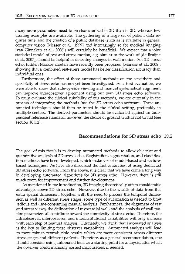
10.5 R£co~\1ENDATIONS FOR 3D STRESS ECHO

many more parameters need to be characterized in 3D than in 2D, whereas few training examples are available. The gathering of a large set of patient data re­qllires time, and the creation of a public database (such as is available in general computer vision [Messer et al., 1999] and increasingly so for medical imaging [van Ginneken et al., 2006]) will certainly be beneficial. We expect that a joint statistical model of rest and stress motion, e.g. similar to the work of [de Bruijne et al., 2007], should be helpful in detecting changes in wall motion. For 2D stress echo, hidden Markov models have recently been proposed [Mansor et al., 2008], showing that a combined rest-stress model has better classification accuracy than individual ones.

Furthermore, the effect of these automated methods on the sensitivity and specificity of stress echo has not yet been investigated. As a first evaluation, we were able to show that side-by-side viewing and manual systematical alignment can improve interobserver agreement using our own 3D stress echo software. To truly evaluate the clinical suitability of our methods, we are currently in the process of integrating the methods into the 3D stress echo software. These au­tomated techniques should then be tested in the clinical setting, preferably in multiple centers. The derived parameters should be evaluated against an inde­pendent reference standard, however, the choice of ground truth is not trivial (see section 10.5.2).

177

Recommendations for 3D stress echo 1.0.5

The goal of this thesis is to develop automated methods to allow objective and quantitative analysis of 3D stress echo. Registration, segmentation, and classifica­tion methods have been developed, which make use of model-based and feature­based techniques. We have also discussed the first evaluation of using dedicated 3D stress echo software. From the above, it is clear that we have come a long way in developing automated algorithms for 3D stress echo. However, there is still much room for improvement and further development.

As mentioned in the introduction, 3D imaging theoretically offers considerable advantages above 2D stress echo. However, due to the wealth of data from this extra spatial dimension, together with the need to process the temporal dimen­sion as well as different stress stages, some type of automation is needed to limit tedious and time-consuming manual analysis. Furthermore, the alignment of rest and stress views, the delineation of myocardial wall, and the analysis of wall mo­tion parameters all contribute toward the complexity of stress echo. Therefore, the intraobserver, interobserver, and interinstitutional variabilities will only increase with each step of manual analysis. Ultimately, we think that automated analysis is the key to limiting these observer variabilities. Automated analysis will lead to more robust, reproducible results which are more consistent across different stress stages and different patients. Therefore, as a general recommendation, one should consider using automated tools as a starting point for analysis, after which the observer could manually correct inaccuracies, if needed.

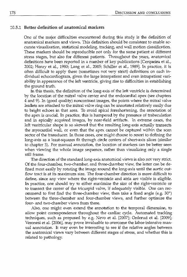
178 DISCUSSION AND CONCLUSIONS

10.5.1 Better definition of anatomical markers

One of the major difficulties encountered during this study is the definition of anatomical markers and views. This definition should be consistent to enable ac­curate visualization, statistical modeling, tracking, and wall motion classification. These markers should be reproducible not only for the same patient at different stress stages, but also for different patients. Throughout the years, anatomical definitions have been reported in a number of key publications [Cerqueira et aL, 2002; Henry et a!., 1980; Lang et al., 2005; Schiller et al., 1989]. In practice, it is often difficult to apply these (sometimes not very strict) definitions on each in­dividual echocardiogram, given the large interpatient and even intrapatient vari­ability in appearance of the left ventricle, giving rise to difficulties in establishing the ground truth.

In this thesis, the definition of the long-axis of the left ventricle is determined by the location of the mitral valve center and the endocardial apex (see chapters 4 and 9). In (good quality) noncontrast images, the points where the mitral valve leaflets are attached to the mitral valve ring can be annotated relatively easily due to bright echoes in that area. To avoid apical foreshortening, the annotation of the apex is cruciaL In practice, this is hampered by the presence of trabeculation and in apically acquired images, by near-field artifacts. In extreme cases, the left ventricular shape is so skewed that the resulting long-axis actually transects the myocardial wall, or even that the apex cannot be captured within the scan sector of the transducer. In those cases, one might choose to resort to defining the long-axis as a least-squares fit through circle centers of short-axis slices (similar to chapter 3). For manual annotation, the location of markers can be better seen when viewing the whole image sequence, rather than visualizing only a single still frame.

The direction of the standard long-axis anatomical views is also not very strict. Of the four-chamber, two-chamber, and three-chamber view, the latter can be de­fined most easily by rotating the image around the long-axis until the aortic out­flow tract is at its maximum size. The four-chamber direction is more difficult to define, since any view where the right-ventricle and atria are visible is eligible. In practice, one should try to either maximize the size of the right-ventricle or to transect the center of the tricuspid valve, if adequately visible. One can rec­ommend to first find the three-chamber view, then take a fixed angle (e.g. 30°) between the three-chamber and four-chamber views, and further optimize the four- and two-chamber views from there.

Also, one might even extend the annotation to the temporal dimension, to allow point correspondence throughout the cardiac cycle. Automated tracking teclmiques, such as proposed by e.g. Nevo et al. [2007]; Orderud et al. [2009]; Veronesi et al. [2006], may prove invaluable to overcome the labor-intensive man­ual annotation. It may even be interesting to see if the relative angles between the anatomical views vary between different stages of stress, and whether this is related to pathology.

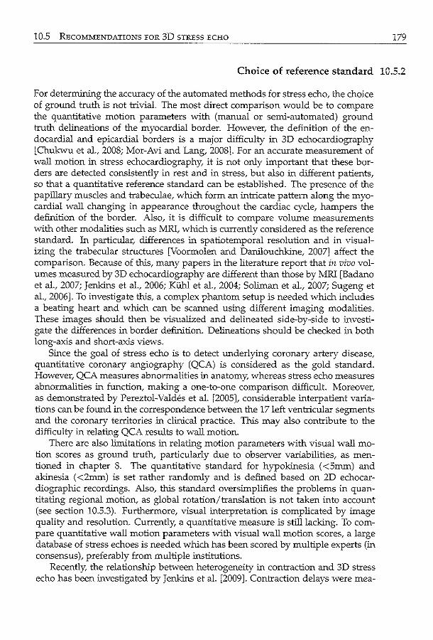
10.5 RECOMMENDATIONS FOR 3D STRESS ECHO 179

Choice of reference standard 10.5.2

For determining the accuracy of the automated methods for stress echo, the choice of ground truth is not trivial. The most direct comparison would be to compare the quantitative motion parameters with (manual or semi-automated) ground truth delineations of the myocardial border. However, the definition of the en­docardial and epicardial borders is a major diliiculty in 3D echocardiography [Chukwu et a!., 2008; Mor-Avi and Lang, 2008]. For an accurate measurement of wall motion in stress echocardiography, it is not only important that these bor­ders are detected consistently in rest and in stress, but also in different patients, so that a quantitative reference standard can be established. The presence of the papillary muscles and trabeculae, which form an intricate pattem along the myo­cardial wall changing in appearance throughout the cardiac cycle, hampers the definition of the border. Also, it is diliicult to compare volume measurements with other modalities such as MRI, which is currently considered as the reference standard. In particular, differences in spatiotemporal resolution and in visual­izing the trabecular structures [Voormolen and Danilouchkine, 2007] affect the comparison. Because of this, many papers in the literature report that in vivo vol­umes measured by 3D echocardiography are different than those by MRI [Badano et a!., 2007; Jenkins et a!., 2006; Kiihl et al., 2004; Soliman et al., 2007; Sugeng et a!., 2006]. To investigate this, a complex phantom setup is needed which includes a beating heart and which can be scanned using different imaging modalities. These images should then be visualized and delineated side-by-side to investi­gate the differences in border definition. Delineations should be checked in both long-axis and short-axis views.

Since the goal of stress echo is to detect underlying coronary artery disease, quantitative coronary angiography (QCA) is considered as the gold standard. However, QCA measures abnormalities in anatomy, whereas stress echo measures abnormalities in function, making a one-to-one comparison difficult. Moreover, as demonstrated by Pereztol-Valdes et a!. [2005], considerable interpatient varia­tions can be found in the correspondence between the 17left ventricular segments and the coronary territories in clinical practice. This may also contribute to the diliiculty in relating QCA results to wall motion.

There are also limitations in relating motion parameters with visual wall mo­tion scores as ground truth, particularly due to observer variabilities, as men­tioned in chapter 8. The quantitative standard for hypokinesia ( <5mm) and akinesia ( <2mm) is set rather randomly and is defined based on 2D echocar­diographic recordings. Also, this standard oversimplifies the problems in quan­titating regional motion, as global rotation/ translation is not taken into account (see section 10.5.3). Furthermore, visual interpretation is complicated by image quality and resolution. Currently, a quantitative measure is still lacking. To com­pare quantitative wall motion parameters with visual wall motion scores, a large database of stress echoes is needed which has been scored by multiple experts (in consensus), preferably from multiple institutions.

Recently, the relationship between heterogeneity in contraction and 3D stress echo has been investigated by Jenkins eta!. [2009]. Contraction delays were mea-

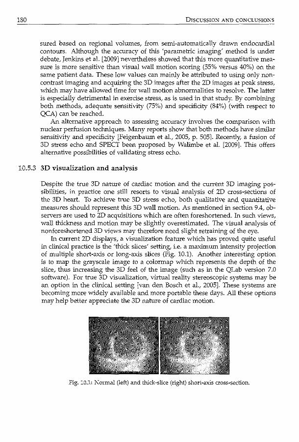
180 DISCUSSION AND CONCLUSIONS

sured based on regional volumes, from semi-automatically drawn endocardial contours. Although the accuracy of this 'parametric imaging' method is under debate, Jenkins et al. [2009] nevertheless showed that this more quantitative mea­sure is more sensitive than visual wall motion scoring (55% versus 40%) on the same patient data. These low values can mainly be attributed to using only non­contrast imaging and acquiring the 3D images after the 2D images at peak stress, which may have allowed time for wall motion abnormalities to resolve. The latter is especially detrimental in exercise stress, as is used in that study. By combining both methods, adequate sensitivity (75%) and specificity (84%) (with respect to QCA) can be reached.

An alternative approach to assessing accuracy involves the comparison with nuclear perfusion techniques. Many reports show that both methods have similar sensitivity and specificity [Feigenbaum et al., 2005, p. 505]. Recently, a fusion of 3D stress echo and SPECT been proposed by Walirnbe et al. [2009]. This offers alternative possibilities of validating stress echo.

10.5.3 3D visualization and analysis

Despite the true 3D nature of cardiac motion and the current 3D imaging pos­sibilities, in practice one still resorts to visual analysis of 2D cross-sections of the 3D heart. To achieve true 3D stress echo, both qualitative and quantitative measures should represent this 3D wall motion. As mentioned in section 9 .4, ob­servers are used to 2D acquisitions which are often foreshortened. In such views, wall thickness and motion may be slightly overestimated. The visual analysis of nonforeshortened 3D views may therefore need slight retraining of the eye.

In current 2D displays, a visualization feature which has proved quite useful in clinical practice is the 'thick slices' setting, i.e. a maximum intensity projection of multiple short-axis or long-axis slices (Fig. 10.1). Another interesting option is to map the grayscale image to a colormap which represents the depth of the slice, thus increasing the 3D feel of the image (such as in the QLab version 7.0 software). For true 3D visualization, virtual reality stereoscopic systems may be an option in the clinical setting [van den Bosch et al., 2005]. These systems are becoming more widely available and more portable these days. All these options may help better appreciate the 3D nature of cardiac motion.

Fig. 10.1: Normal (left) and thick-slice (right) short-a.'Xis cross-section.

10.5 RECOMME:NDATIONS FOR 3D STRESS ECHO

For analysis of stress echo, it may be an option to visualize rest and stress im­ages superimposed on each other, color-coded to different color channels and syn­chronized in time, to better emphasize the differences in motion. A fine checker­board representation (like in Fig. 4.5) may also be beneficial.

For quantitative analysis, wall motion should of course be measured in 3D. One may choose to use an implicit statistical method as proposed in chapter 8 for modeling this motion, or one may opt to explicitly model individual segments. When explicitly defining segmental wall motion, it is important to choose a good spatial reference point, to distinguish between the global rotation/ translation mo­tion of the heart and local behavior [Marwick, 2003, p. 55]. This is not a trivial task. Poor definition may result in the estimated motion of segments opposite one an­other to affect each other, in cases with severe wall motion abnormality. Probably it is more interesting to quantify the differences between rest and stress motion per patient, instead of dealing with these stages separately.

It would be interesting to incorporate a measure of certainty in the interpreta­tion and visualization of results of automated methods. Since ultrasound images often contain artifacts that limit the analysis, areas where e.g. contours could not be detected properly should be indicated as such, for example using dotted or transparent lines. Chapter 7 is an example of such a measure. This should help not only the quantitative analysis but also the visual interpretation of the auto­matically detected results.

181

Real-time processing 10.5.4

ln recent years, there has been an increasing interest in developing analysis meth­ods for (near) real-time analysis, which can be incorporated into the ultrasound machines. Currently, methods focus on e.g. state estimation [Hansegard et al., 2007a; Orderud et al., 2007b] and machine learning schemes [Lu et al., 2008; Yang et al., 2008b], which have low computational costs. However, it is always impor­tant to keep in mind whether these methods sacrifice accuracy for speed. To really compete with the clinical workflow of 2D stress echo, anatomical view selection methods are needed at the very least, and these should run at (near) real-time. In­stead of choosing methods with low computational cost, one could also optimize existing methods (e.g. using multiscale techniques), or use smart implementation techniques (e.g. parallel processing, or gpu-based implementations).

Another interesting research area is the development of real-time artifact de­tection methods. These may be used to give direct feedback on the optimality of acquisition. For example, Orderud et al. [2007a] have reported on real-time detection of poor acoustic contact of the probe on the patient's skin. Such meth­ods could potentially be used to optimize the probe position during acqulsition. The real-time detection and visualization of anatomical views may also help to pre-align rest and stress images as much as possible during acquisition.

182 DISCUSSION AND CONCLUSIONS

10.6 Future directions

1().6.1 Improvements 3D stress echo

When 3D stress echocardiography was first introduced at the beginning of this decade, it was received with much enthusiasm. Of the reports on dobutamine stress echo, only a few studies [Aggeli eta!., 2007; Ahmad et al., 2001; Krenning et a!., 2008; Matsumura et al., 2005] compared 3D stress with coronary angiog­raphy. These studies reported sensitivity (61%-88%) and specificity (80%-89%) values in detecting coronary artery disease, which are in the range of 2D studies (average sensitivity=83% and specificity=83%, [Krenning et al., 2004]). Despite these encouraging reports, clinical routine application of stress echocardiography is still limited, due to the yet unsolved problems of spatiotemporal resolution, image quality, time-consuming manual analysis (as discussed in section 10.5), and lack of stress specific acquisition protocols. Until these issues are sufficiently addressed, it is difficult to evaluate the true value of 3D stress echocardiography.

Spatiotemporal resolution

Despite the advances in transducer technology in recent years, the spatiotemporal resolution and image quality of 3D echocardiography is still inferior to that of 2D echocardiography. Currently, a very promising development is single heart-beat imagjng. Using smart beamforming and signal processing teclmiques, the whole left ventricle can be acquired within one cardiac cycle, without volume stitching. This will eliminate the motion artifacts due to beat-to-beat variations. For stress sequences, improvement of temporal resolution may be more important than that of spatial resolution, because these sequences are generally shorter than the rest sequences due to the higher heart rate. Preferably, the frame rate should be at least 30 frames per second [Lang et al., 2005].

Image quality

Ultrasound artifacts form a considerable problem in the analysis of echocardio­grams. In practice, the visibility of myocardial wall segments in stress images is inferior to that of the rest image in the same patient [Krenning et al., 2008; Nemes et al., 2007b]. More research is needed to deal with these artifacts, not only using image post-processing methods, but also with improvements in hardware. The use of higher harmonics and smart pulsing schemes may prove useful here. Also, effort should be put into (further) reducing the footprint of the transducer, for optimal transthoracic imaging.

10.6 FUTURE DIRECTIONS

Stress specific acquisition protocol

To enable routine use of 3D imaging for stress echo, dedicated protocols for ac­quisition of stress images should be available on the ultrasound machine. Several commercial companies have very recently included or are on the verge of intro­ducing these protocols. At the very least, these protocols should allow side-by­side viewing of all stages (to optimize anatomical alignment during acquisition), easy switching between acquisition environment of the 2D and 3D transducer, simple labeling of different stress stages during acquisition, and exporting to of­fline analysis. All these things seem quite trivial but are essential in enabling 3D stress echo in clinical routine practice.

Also, the machine settings should be optimized for stress to improve frame rate: the scan sector should be as narrow as possible, and the imaging depth should also be set so that only the left ventricle is captured (and not too much of the atrium). There should also be separate settings for contrast-enhanced imaging so that one can switch easily between noncontrast and contrast acquisition, while maintaining a high frame rate.

Alternative approaches to automated analysis

In this thesis, we have chosen to tackle automated stress echo via initialization, segmentation, and classification approaches, using registration, model-based, and data-driven techniques. Recently, new machine learning methods have been pro­posed, based on marginal space learning and probabilistic boosting tree, which can be adapted to solve all three problems. These methods involve construction of extensive databases of the object to be analyzed using a simple, overcomplete set of features. The approach was inspired by the work of Viola and Jones [2001] for detecting faces in photographic images, and has very recently been extended to medical applications [Carneiro et al., 2008; Georgescu et al., 2005; Zheng et a!., 2008]. This promising method appears to be quite robust, accurate and fast (in the order of a few seconds), as demonstrated by Georgescu et al. [2005] and Yang eta!. [2008b]. However, it does require many annotated training samples, many more than the statistical model-based approaches. The application to stress echo analysis remains to be investigated, and ways of artificially augmenting the database definitely requires further attention.

183

Stress and contrast 10.6.2

Reports in the literature show that contrast can improve visibility of the my­ocardium, resulting in more segments which can be analyzed via visual wall motion scoring in 3D [Nemes eta!., 2007b]. Therefore, future work should evolve around methods for analyzing contrast images. In chapter 6, we presented some preliminary work on segmentation of contrast echocarcliograms. The swirling patterns and inflow and outflow of contrast in the left ventricular cavity cause differences in image intensity between each acquisition, which are difficult to capture within model-based analysis. On the other hand, feature-based methods

184 DISCUSSION AND CONCLUSIONS

may be able to exploit these fast varying patterns for distinguishing contrast from myocardium in segmentation methods. Also, segmentation of the mitral valve requires more attention, since this structure is less clearly visible in contrast en­hanced images due to attenuation by the contrast media. Given the differences between noncontrast and contrast-enhanced imaging, it can be envisioned that the analysis of contrast images requires the development of dedicated methods, which is a subject of further research.

Another application of contrast echocardiography which is quickly gaining in­terest is myocardial perfusion [Dijkmans et al., 2006]. This technique examines the speed and extent of contrast inflow into the microvasculature in the myocardium. Within a stress echo setting, studies have concentrated on detecting stable coro­nary artery disease and for detecting acute coronary syndromes. For automated analysis of these images, multimodality registration and classification approaches may be promising [Slomka et al., 2004].

10.6.3 Other quantitative measures

3D strain and strain-rate imaging has also become an interesting topic of research. In the past decade, 2D speckle tracking methods have been developed for estimat­ing the in-plane strain in the left ventricular myocardium [Helle-Valle et al., 2005]. Speckle tracking methods can potentially be used for assessing myocardial defor­mation in stress echo [Govind et al., 2009; Moonen et al., 2009; Reant et al., 2008]. These speckle tracking methods are usually based on block-matching and optical­flow approaches. Since the heart is a moving 3D structure, the through-plane mo­tion of the heart may cause speckle patterns in 2D images to become decorrelated. True 3D speckle tracking can overcome this limitation. However, the i¢erior spa­tial and temporal resolution and overall image quality pose technical challenges which need to be resolved before 3D speckle tracking can be applied in clinical practice. Nevertheless, preliminary clinical studies show promising results in 3D [Kawagishi, 2008; Nesser and Wmter, 2009].

Besides motion, myocardial wall thickening is an important parameter for as­sessing normal and abnormal contractility. A way to measure wall thickening is to detect both the epicardium and the endocardium. Segmentation of these borders has been investigated more extensively for CT and MR images. Recently, auto­mated 3D epicardium detection has been investigated [Walimbe et al., 2006; Zhu et al., 2007], which make use of spatial constraints based on the location of the en­docardium. Epicardium segmentation is more challenging, particularly in apical views [Noble and Boukerroui, 2006], due to the limited visibility and suboptimal spatial resolution.

10.7 Conclusions

In this thesis, automated methods have been proposed for quantitative and ob­jective analysis of 3D stress echocardiography. These methods are used to ini-

10.7 CONCLUSIONS

tialize anatomical markers and views, to obtain endocardial borders throughout the cardiac cycle, and to automatically detect wall motion abnormalities based on endocardial border information. These methods cover a wide range of techniques from medical image processing, including registration, segmentation, and classifi­cation approaches, using both low-level feature-based and high-level model-based techniques. Also, a dedicated software package is developed for clinical routine practice, which has been shown in a first clinical study to have significant ben­efits for reducing interobserver variability, one of the major limitations in stress echo. Thus, we have shown that considerable advances have been made to allow a more robust and accurate analysis, which, we hope, will also improve the clinical workflow and feasibility of 3D stress echo.

From the above discussion, we have seen that the combination of low level and high level image information is crucial for obtaining robust clinical parameters. This is especially relevant in the analysis of ultrasound images, where image quality is more challenging than e.g. in MR or CT. Also, we anticipate that the combination of all available image information via registration, segmentation and classification, should enhance the performance of stress echo as a whole.

As discussed in the previous sections, many opportunities remain for improv­ing automated analysis of 3D stress echo. The presented methods should be evaluated as a whole. The classification of wall motion in 3D still requires further investigation, as well as the effect of automation on sensitivity and specificity of 3D stress echo. Some key issues still need to be addressed, such as better defi­nition of anatomy, 3D visualization and analysis, and the possibility of real-time processing. Future research opportunities remain for contrast imaging and inte­gration of other meaningful quantitative measures. This could further enhance the robustness and accuracy of 3D stress echo.

Besides dedicated research, the development of dedicated software and ac­quisition protocols are crucial for boosting automated methods to clinical prac­tice. For thorough clinical evaluation, implementation of the proposed methods is needed. The development of a user-friendly interface is an important part in this process, which requires regular contact with clinical experts. In addition, through closer collaboration, commercial companies can expedite the testing and application of automated methods through inclusion in their own software.

Given the wealth of data in 3D imaging, we anticipate that automated meth­ods will be invaluable for improving clinical workflow and reducing observer variabilities. The automated methods should give a complete, precise report of the function of the left ventricle. The methods developed in this thesis aim at providing useful quantitative and objective clinical parameters, as well as at im­proving the overall clinical workflow. However, it is important to remark that the automated methods are a tool for helping the decision making process of the clin­ical expert. Ultimately, the final diagnosis should be provided by the cardiologist.

185

References

Aggeli, C., G. Giarmopoulos, P. Misovoulos, G. Roussakis, E. Christoforatou, C. Kokki­nakis, S. Brili, and C. Stefanadis [2007]. Real-time three-dimensional dobutaroine stress echocardiography for coronary artery disease diagnosis: Validation with coronary an­giography. Heart. 93 (6). 672-5.

Ahmad, M., T. Xie, M. McCulloch, G. Abreo, and M. Runge [2001]. Real-time three­dimensional dobutamine stress echocardiography in assessment of ischemia: Compar­ison with two-dimensional dobutaroine stress echocardiography. J. Am. Coli. Cardiol. 37 (5). 1303-9.

Altman, D. G. [1997]. Practical statistics for medical research. 1st edition. London: Chapman and Hall.

Amini, A. A., T. E. Weymouth, and R. C. Jain [1990]. Using dynamic programming for solv­ing variational problems in vision. IEEE Trans. Pattern Anal. Mach. Intel!. 12. 855--{;7.

Angelini, E. D. and 0. Gerard [2006]. Review of myocardial motion estimation methods from optical flow tracking on ultrasound data. Proc. IEEE Eng Med Bioi Soc. 1537-40.

Angelini, E. D., A. F. Laine, S. Takuma, J. W. Holmes, and S. Homma [2001]. LV vol­ume quantification via spatiotemporal analysis of real-time 3D echocardiography. IEEE Trans. Med. Imaging. 20 (6). 457--<i9.

Angelini, E. D., S. Homma, G. Pearson, J. W. Hoimes, and A. F. Laine [2005]. Segmentation of real-time three-dimensional ultrasound for quantification of ventricular function: A clinical study on right and left ventricles. Ultrasound Med. Bioi. 31 (9). 1143-58.

Aoued, F., E. Eroglu, L. Herbots, F. Rademakers, and J. D'hooge [2005]. A statistical model­based approach for the detection of abnormal cardiac deformation. Proc. IEEE Int. Ultrason. Symp. 512-5.

188 REFERENCES

Armstrong, G., A. Pasquet, K. Fukamachi, L. Cardon, B. Olstad, and T. Marwick [2000]. Use of peak systolic strain as an index of regional left ventricular function: Comparison with tissue Doppler velocity during dobutarnine stress and myocardial ischemia. J. Am. Soc. Echocardiogr. 13 (8). 731-7.

Armstrong, W. F. and W. A. Zoghbi [2005]. Stress echocardiography: Current methodology and clinical applications. J. Am. Coli. Cardiol. 45 (11). 1739-47.

Amese, M., P. M. Fioretti, J. H. Cornel, J. Postma-Tjoa, A. E. M. Reijs, and J. R. T. C. Roelandt [1994]. Akinesis becoming dyskinesis during high-dose dobutamine stress echocardiography: A marker of myocardial ischemia or a mechanical phenomenon? Am. J. Cardiol. 73 (12). 896-9.

Arulampalam, M. S., S. Maskell, N. Gordon, and T. Clapp [2002]. A tutorial on particle filters for online nonHnear I non-Gaussian Bayesian tracking. IEEE Trans. Signal Process. 50 (2). 174-88.

Assmann, P. E., C. J. Slager, S. G. van der Borden, J. G. P. Tijssen, J. A. Oomen, and J. R. Roelandt [1993]. Comparison of models for quantitative left ventricular wall motion analysis from tvvo-dimensional echocardiograms during acute myocardial infarction. Am. J. Cardiol. 71 (15). 1262-9.

Audette, M. A., F. p_ Ferrie, and T. M. Peters [2000]. An algorithmic overview of surface registration teclmiques for medical imaging. Med. Image Anal. 4 (3). 201-17.

Badano, L. P., E. Dall' Armellina, M. J. Monaghan, M. Pepi, M. Baldassi, M. Cinello, and P. M. Fioretti [2007]. Real-time three-dimensional echocardiography: Technological gad­get or clinical tool? J. Cardiovasc. Med. 8 (3). 144--62.

Ballard, D. H. [1981]. Generalizing the hough transform to detect arbitrary shapes. Pattern Recogn. 13 (2). 111-22.

Baraldi, P., A. Sarti, C. Lamberti, A. Prandini, and F. Sgallari [1996]. Evaluation of differen­tial optical flow techniques on synthesized echo images. IEEE Trans. Biomed. Eng. 43 (3). 259-72.

Barnett, S. B., G. R. ter Haar, M. C. Ziskin, H. D. Rott, F. A. Duck, and K. Maeda [2000]. International recommendations and guidelines for the safe use of diagnostic ultrasound in medicine. Ultrasound Med. Bioi. 26 (3). 355-<i6.

Barron, J. L., D. J. Fleet, and S. S. Beauchemin [1994]. Performance of optical flow tech­niques. Int. J. Comput. Vis. 12 (1). 43--77.

Batur, A. U. and M. H. Hayes [2005]. Adaptive active appearance models. IEEE Trans. Image Process. 14 (11). 1707-21.

Bay, H., A. Ess, T. Tuytelaars, and L. van Goo! [2008]. Speeded-up robust features (SURF). Comput. Vis. Image Und. 110 (3). 34&-59.

Behar, V., D. Adam, P. Lysyansky, and Z. Friedman [2004]. Improving motion estimation by accounting for local image distortion. Ultrasonics. 43. 57-65.

Beichel, R., H. Bischof, F. Leber!, and M. Sonka [2005]. Robust active appearance models and their application to medical image analysis. IEEE Trans. Med. Imaging. 24 (9). 1151-69.

REFERENCES

Belaroussi, B., J. Milles, S. Carme, Y. M. Zhu, and H. Benoit-Catlin [2006]. lntensity non­uniformity correction in MRI: Existing methods and their validation. Med.lmage Anal. 10 (2). 234-46.

Bellmann, R. E. [1965]. Dynamic programming. Princeton University Press.

Bermejo, )., ). Timperley, R. G. Odreman, M. Mulet, ). A. Noble, A. P. Banning, R. Yotti, E. Perez-David, J. Declerck, H. Becher, and M. A. Garda-Fernandez [2008]. Objective quantification of global and regional left ventricular systolic function by endocardial tracking of contrast echocardiographic sequences. lnt. ). Cardiol. 124 (1). 47-56.

Birchfield, S. and C. Tomasi [1998]. A pixel dissimilarity measure that is insensitive to image sampling. IEEE Trans. Pattern Anal. Mach. lntell. 20 ( 4). 401-6.

Birchfield, S.T. [1999]. Depth and motion discontinuities. Ph.D. Thesis. Stanford University.

Bjaerum, 5., H. Torp, and K. Kristoffersen [2002]. Clutter filters adapted to tissue motion in ultrasound color flow imaging. IEEE Trans. Ultrason. Ferroelectr. Freq. Control. 49 (6). 693-704.

Black, M. ). and P. Anandan [1996]. The robust estimation of multiple motions: Pararneteric and piecewise-smooth flow fields. Comput. V!s.lmage Und. 63 (1). 75-104.

Bland,). M. and D. G. Altman [1986]. Statistical methods for assessing agreement between two methods of clinical measurement. Lancet. 327 (8476). 307-10.

Bogaert, J. G., H. T. Bosmans, F. E. Rademakers, E. P. Bellon, M. C. Herregods, J. A. Ver­schakelen, F. van de Werf, and G.). Marchal [1995]. Left ventricular quantification with breath-hold MR imaging: Comparison with echocardiography. Magma. 3 (1). 5-12.

Bosch, H. G., G. van Burken, F. Nijland, and ). H. C. Reiber [1998]. Overview of auto­mated quantitation techniques in 2D echocardiography.ln: What's new in cardiovascular imaging? Ed. by J. H. C. Reiber and E. E. van der Wall. Kluwer Academic Publishers, 363-76.

Bosch, J. G., S. C. Mitchell, B. P. F. Lelieveldt, F. Nijland, 0. Karnp, M. Sonka, and ). H. C. Reiber [2002]. Automatic segmentation of echocardiographlc sequences by active appearance motion models. IEEE Trans. Med.lmaging. 21 (11). 1374--83.

Bosch,). G., F. Nijland, S. C. Mitchell, B. P. F. Lelieveldt, 0. Kamp, ). H. C. Reiber, and M. Sonka [2005]. Computer-aided diagnosis via model-based shape analysis: Automated classification of wall motion abnormalities in echocardiograms. Acad. Radiol. 12 (3). 358-67.

Bosch,). G., M. van Stralen, M. M. Voorrnolen, B. J. Krenning, C. T. Lancee, J. H. C. Reiber, A. F. W. van der Steen, and N. de Jong [2006]. Novel spatiotemporal voxel interpolation with multibeat fusion for 3D echocardiography with irregular data distribution. Proc. SPlE Med. lmaging. 6147. 61470Q.

Boukerroui, D., A. Baskurt, ). A. Noble, and 0. Basset [2003]. Segmentation of ultrasound images - multiresolution 2D and 3D algorithm based on global and local statistics. Pattern Recogn. Lett. 24. 779-90.

Boykov, Y., 0. Veksler, and R. Zabth [2001]. Fast approximate energy minimization via graph cuts. lEEE Trans. Pattern Anal. Mach. lntell. 23 (11). 1222-39.

189

190 REFERENCES

Brekke, S., S. I. Rabben, A. Stoylen, A. Haugen, G. U. Haugen, E. N. Steen, and H. Torp [2007]. Volume stitchlng in three-dimensional echocardiography: Distortion analysis and extension to real time. Ultrasound Med. Bioi. 33 (5). 782-96.

Browne, M. W. [2001]. An overview of analytic rotation in exploratory factor analysis. Multivar. Behav. Res. 36 (1). 111-50.

Broyden, C. [1976]. A class of methods for solving nonlinear simultaneous equations. Proc. Math. Comput. 30. 1-17.

Bruhn, A.,). Weickert, and C. Schnorr [2005]. Lucas/Kanade meets Horn/Schunck: Com­bining local and global optic flow methods. Int.). Comput. Vision. 61 (3). 211-31.

Buades, A., B. Coil, and). M. Morel [2000]. A review of image denoising algorithms, with a new one. Multiscale Model Simul. 4 (2). 490-530.

Burt, P. ). and E. H. Adelson [1983]. The Laplacian pyramid as a compact image code. IEEE Trans. Commun. COM-31 (4). 532-40.

Bylund, N. E., M. Andersson, and H. Knutsson [2005]. Interactive 3D filter design for ultrasound artifact reduction. Proc. IEEE Int. Conf. lmage Process. 3. 728-Jl.

Caiani, E. G., C. Corsi,). Zamorano, L. Sugeng, P. MacEneaney, L. Weinert, R. Battani, ). L. Gutierrez, R. Koch, L. Perez de Isla, V. Mor-Avi, and R. M. Lang [2005]. Improved semiautomated quantification of left ventricular volumes and ejection fraction using 3-dim.ensional echocardiography with a full matrix-array transducer: Comparison with magnetic resonance imaging.). Am. Soc. Echocardiogr. 18 (8). 779-88.

Cameiro, G., B. Georgescu, S. Good, and D. Comaniciu [2008]. Detection and measurement of fetal anatomies from ultrasound images using a constraiDed probabilistic boosting tree. IEEE Trans. Med. Imaging. 27 (9). 1342-55.

Cerqueira, M. D., N. ). Weissman, V. Dilsizian, A. K. jacobs, S. Kaul, W. K. Laskey, D. j. Pennell, ). A. Rumberger, T. Ryan, and M Verani [2002]. Standardized myocardial segmentation and nomenclahlre for tomographic imaging of the heart. Circulation. 105 (4). 539-42.

Chan, K. L., X. Liu, K. ). Ascah, L. M. Beauchesne, and I. G. Burwash [2004]. Comparison of real-time 3-dimensional echocardiography with conventional 2-dimensional echo­cardiography in the assessment of structural heart disease. J. Am. Soc. Echocardiogr. 17 (9). 976-<30.

Chukwu, E. 0., E. Barasch, D. G. Milialatos, A. Katz, j. Lachmann, ). Han, N. Reichek, and A. S. Gopal [2008]. Relative importance of errors in left ventricular quantitation by two-dimensional echocardiography: Insights from three-dimensional echocardiogra­phy and cardiac magnetic resonance imaging.). Am. Soc. Echocardiogr. 21 (9). 990-7.

Chunke, Y., K. Terada, and S. Oe [1996]. Motion analysis of echocardiograph using optical flow method. Proc. IEEE Int. Conf. Systems, Man and Cybernetics. 1. 672-7.

Cloutier, G., D. Chen, and L. G. Durand [2003]. A new clutter rejection algorithm for Doppler ultrasound. IEEE Trans. Med. Imaging. 22 (4). 530-S.

Cobbold, R. S. C. [2007]. Foundations of biomedical ultrasound. New York: Oxford University Press.

REFERENCES

Cohen, B. and I. Dinstein [2002]. New maximum likelihood motion estimation schemes for noisy ultrasound images. Pattern Recogn. 35 (2). 455-63.

Comaniciu, D., X. S. Zhou, and S. Krishnan [2004]. Robust real-time myocardial border tracking for echocardiography: An information fusion approach. IEEE Trans. Med. Imaging. 23 (7). 849-<iO.

Comte, A., A. Lalande, S. Aho, P.M. Walker, and F. Brunette [2004]. Realignment of myo­cardial first-pass MR perfusion images using an automatic detection of the heart-lung interface. Magn. Reson. Imaging. 22 (7). 1001-9.

Coates, T. F. and P. Kittipanya-ngam [2002]. Comparing variations on the active appearance model algorithm. Proc. Br. Mach. Vis. Conf. 2. 837-46.

Coates, T. F. and C. J. Taylor [1999]. A rrilxture model for representing shape variation. Image Vis. Comput. 17 (8). 567-73.

Coates, T. F. and C. J. Taylor [2006]. An algorithm for tuning an active appearance model to new data. Proc. Br. Mach. Vis. Conf. 3. 919-28.

Coates, T. F., G. J. Edwards, and C. J. Taylor [1998]. Active appearance models. Proc. Eur. Conf. Comput. Vis. 2. 484-98.

Coates, T. F., G. J. Edwards, and C. J. Taylor [2001]. Active appearance models. IEEE Trans. Pattern Anal. Mach. Intel!. 23 (6). 681-5.

Coates, T. F., D. H. Cooper, C. J. Taylor, and J. Graham [1992]. Trainable method of para­metric shape-description. Image Vis. Comput. 10 (5). 289-94.

Corsi, C., G. Saracino, A. Sarti, and C. Lamberti [2002]. Left ventricular volume estimation for real-time three-dimensional echocardiography. IEEE Trans. Med. Imaging. 21 (9). 1202-8.

Corsi, C., R. M. Lang, F. Veronesi, L. Weinert, E. G. Caiani, P. MacEneaney, C. Lamberti, and V. Mor-A vi [2005]. Volumetric quantification of global and regional left ventricular function from real-time three-dimensional echocardiographic images. Circulation. 112 (8). 1161-70.

Costen, N. P., T. F. Coates, G. J. Edwards, and C. J. Taylor [2002]. Automatic extraction of the face identity-subspace. Image Vis. Comput. 20 (5-6). 319-29.

Crawford, C. B. and G. A. Ferguson [1970]. A general rotation criterion and its use in orthogonal rotation. Psychometrika. 35 (3). 321-32.

Dalal, N. and B. Triggs [2005]. Histograms of oriented gradients for human detection. Proc. IEEE Conf. Comput. Vis. Pattern Recogn. 2. 886-93.

Danilouchkine, M. G., J. J. Westenberg, H. C. van Assen, J. H. C. Reiber, and B. P. F. Lelieveldt [2005]. 3D model-based approach to lung registration and prediction of res­piratory cardiac motion. Proc. Med. Image Comput. Comput. Assist. Interv. LNCS 3750. 951-59.

Danilouchkine, M. G., F. Mastik, and A. F. W. van der Steen [2008]. Accuracy in prediction of catheter rotation in IVUS with feature-based optical flow- a phantom study. IEEE Trans. Jnf. Techno!. Biomed. 12 (3). 355-65.

De !a Torre, F. and M. J. Black [2003]. A framework for robust subspace learning. Int. J. Comput. Vis. 54. 117-42.

191

192 REFERENCES

De Bruijne, M., M. T. Lund, L. B. Tanko, P. C. Pettersen, and M. Nielsen [2007]. Quantitative vertebral morphometry using neighbor-conditional shape models. Med. Image Anal. 11 (5). 503-12.

DeCara, J. M., V. Mor-Avi, L. Weinert, C. E. Korcarz, K. A. Collins, K. T. Spencer, J. E. Bednarz, and R. M. Lang [2004]. Automated quantitative assessment of wall motion in patients with poor acoustic windows. J. Am. Soc. Echocardiogr. 17 (7). 723-31.

Declerck, J., J. Feldmar, M. L. Goris, and F. Betting [1997]. Automatic registration and alignment on a template of cardac stress and rest reoriented SPECT images. IEEE Trans. Med. Imaging. 16 (6). 727-37.

Delzescaux, T., F. Frouin, A. de Cesare, S. Philipp-Foliguet, A. Todd-Pokropek, A. Her­ment, and M. Janier [2003]. Using an adaptive serniautomated self-evaluated regis­tration technique to analyze 1v1Rl data for myocardial perfusion assessment. J. Magn. Reson.lmaging. 18 (6). 681-90.

Dempster, A. P., N. M. Laird, and D. B. Rubin [1977]. Maximum likelihood from incomplete data via the EM algorithm. J. R. Stat. Soc. Ser. B (Methodol.) 39 (1). 1-38.

Dijkmans, P. A., R. Senior, H. Becher, T. R. Porter, K. Wei, C. A. Visser, and 0. Kamp [2006]. Myocardial contrast echocardiography evolving as a clinically feasible technique for accurate, rapid, and safe assessment of myocardial perfusion: The evidence so far. J. Am. Coli. Cardiol. 48 (11). 2168-77.

Dougherty, L., J. C. Asmuth, A. S. Blom, L. Axel, and R. Kumar [1999]. Validation of an optical flow method for tag displacement estimation. IEEE Trans. Med. Imaging. 18 (4). 359-63.

Drake, R. L., W. Vogl, and A. W. M. Mitchell [2005]. Gray's anatomy for students. Philadel­phia, PA: Elsevier.

Duan, Q., E. D. Angelini, S. L. Herz, C. M. Ingrassia, K. D. Costa, J. W. Holmes, S. Horruna, and A. F. Laine [2008]. Region-based endocardium tracking on real-time three­dimensional ultrasound. Ultrasound Med. Biol. 35 (2). 256-65.

Duarte, M. A., J. C. Machado, and W. C. A. Pereira [2003]. A method to identify acoustic reverberation in multilayered homogeneous media. U1trasonics. 41. 683-98.

Duck, F. A. [2002]. Nonlinear acoustics in diagnostic ultrasound. Ultrasound Med. Bioi. 28 (1). 1-18.

Elen, A., H. F. Choi, D. Loeckx, H. Gao, P. Claus, P. Suetens, F. Maes, and J. D'Hooge [2008]. Three-dimensional cardiac strain estimation using spatio-temporal elastic registration of ultrasound images: A feasibility study. IEEE Trans. Med. Imaging. 27 (11). 1580-91.

Elhendy, A., R. T. van Domburg, J. J. Bax, D. Poldermans, P.R. Nierop, J.D. Kasprzak, and J. R. T. C. Roeland! [1998]. Optimal criteria for the diagnosis of coronary artery disease by dobutamine stress echocardiography. Am. J. Cardiol. 82 (11). 1339-44.

Eto, Y., H. Yamada, J. H. Shin, D. A. Agler, H. Tsujino, J. X. Qin, G. Saracino, N. L. Green­berg, J. D. Thomas, and T. Shiota [2005]. Automated mitral annular tracking: A novel method for evaluating mitral annular motion using two-dimensional echocardiogra­phy. J. Am. Soc. Echocardiogr. 18 (4). 306-12.

REFERENCES

Fei, B., ). L. Duerk, D. T. Boll,). S. Lewin, and D. L. Wilson [2003]. Slice-to-volume reg­istration and its potential application to interventional MRI-guided radio-frequency thermal ablation of prostate cancer. IEEE Trans. Med. Imaging. 22 (4). 515-25.

Feigenbaum, H., W. F. Armstrong, and T. Ryan [2005]. Feigenbaum's echocardiography. 6th edition. Philadelphia: Lippincott WJ.!liams & Wilkins.

Firmin~ D. and J. Keegan [2001]. Navigator echoes in cardiac magnetic resonance. J. Car­diovasc. Magn. Reson. 3 (3). 183-93.

Fischler, M.A. and R. C. Bolles [1981]. Random sample consensus: A paradigm for model fitting with applications to image analysis and automated cartography. Commun. ACM. 24. 381-95.

Florack, L. M. J., H. C. van Assen, and A. Suinesiaputra [2007]. Dense multiscale motion extraction from cardiac cine MR tagging using HARP technology. Proc. Int. Con£. Com­put. Vis. Workshop Math. Methods Biomed. Image Anal. 2838-45.

Foroughi, P. and P. Abolmaesumi [2006]. Intra-subject elastic registration of 3D ultrasound images. Med. Image Anal. 10. 713-25.

Frouin, F., A. Delouche, H. Raffoul, H. Diebold, E. Abergel, and B. Diebold [2004]. Factor analysis of the left ventricle by echocardiography (FALVE): A new tool for detecting regional wall motion abnormalities. Eur. ). Echocardiogr. 5 (5). 335-46.

Fujino, T., S. Ono, K. Murata, N. Tanaka, T. Tone, T. Yamamura, Y. Tomochika, K. Kllnura, K. Ueda, ). Liu, Y. Wada, M. Murashita, Y. Kondo, and M. Matsuzaki [2001]. New method of on-line quantification of regional wall motion with automated segmental motion analysis.). Am. Soc. Echocardiogr. 14 (9). 892-901.

Fung, G., M. Qazi, S. Krishnan, ). Bi, and B. Rao [2005]. Sparse classifiers for auto­mated heart wall motion abnormality detection. Proc. Int. Conf. Mach. Learning Appl. 194-200.

Garcia-Fernandez, M.A., I- Bermejo, E. Perez-David, T. Lopez-Femandez, M. J. Ledesma, P. Caso, N. Malpica, A. Santos, M. Moreno, and M. Desco [2003]. New techniques for the assessment of regional left ventricular wall motion. Echocardiography. 20 (7). 659-72.

Geleijnse, M. L., P. M. Fioretti, and). R. Roeland! [1997]. Methodology, feasibility, safety and diagnostic accuracy of dobutamine stress echocardiography. ). Am. Col!. Cardiel. 30 (3). 595-606.

Georgescu, B., X. S. Zhou, D. Comaniciu, and A. Gupta [2005]. Database-guided segmenta­tion of anatomical structures with complex appearance. Proc. IEEE Conf. Comput. VlS. Pattern Recogn. 2. 429-36.

Gerard, 0., A. C. Billon, ).-M. Rouet, M. Jacob, M. Fradkin, and C. Allouche [2002]. Efficient model-based quantification of left ventricular function in 3-D echocardiography. IEEE Trans. Med. Imaging. 21 (9). 1059-{;8.

Gerig, M., G. Jomier, and M. Chakos [2001]. Valmet: A new validation tool for assessing and improving 3D object segmentation. Proc. Med. Image Comput. Comput. Assist. Interv. LNCS 2208. 516-23.

Giachetti, A. [2000]. Matching techniques to compute image motion. Image Vis. Comput. 18 (3). 247--<iO.

193

194 REFERENCES

Golemati, S., J. Stoitsis, E. G. Sifakis, T. Balkizas, and K. S. Nikita [2007]. Using the hough transform to segment ultrasound images of longitudinal and transverse sections of the carotid artery. Ultrasound Med. Biol. 33 (12). 1918-32.

Gorce, J.-M., D. Friboulet, and I. E. Magnin [1997]. Estimation of three-climensional car­diac velocity ·fields: Assessment of a differential method and application to three­dimensional CT data. Med. Image Anal. 1 (3). 245-61.

Govind, S. C., A. S. Gopal, A. Netyo, J. Nowak, L. A. Brodin, A. Patrianakos, S. S. Ramesh, and S. Saha [2009]. Quantification of low-dose dobutamine stress using speckle tracking echocardiography in coronary artery disease. Eur. J. Echocardiogr. 10 (5). 607-12.

Gower, J. C. [1975]. Generali.7""d procrustes analysis. Psychometrika. 40 (1). 33-51.

Grau, V. and J. A. Noble [2005]. Adaptive multiscale ultrasound compounding using phase information. Proc. Med. Image Comput. Comput. Assist. Interv. LNCS 3749. 589-96.

Grau, V., H. Becher, and J. A. Noble [2006]. Phase-based registration of multi-view real-time three-dimensional echocardiographic sequences. Proc. Med. Image Comput. Comput. Assist. Interv. LNCS 4190. 612-9.

Gray, H. [1918]. Gray's anatomy of the human body. 20th edition. Philadelphia, PA: Lea & Febiger.

Gross, R., I. Matthews, and S. Baker [2004]. Constructing and fitting active appearance models with occlusion. Proc. IEEE Con£. Comput. Vision Pattern Recognit. 5. 72-80.

Gupta, S. N., M. Solaiyappan, G. M. Beache, A. E. Arai, and T. K. Foo [2003]. Fast method for correcting image misregistration due to organ motion in time-series 1v1Rl data. Magn. Reson. Med. 49 (3). 506--14.

Guyton, A. C. and J. E. Hall [1996]. Textbook of medical physiology. Philadelphia: W. B. Saun­ders Company.

Hadjidemetriou, S., C. Studholme, S. Mueller, M. Weiner, and N. Schuff [2009]. Restoration of 1v1Rl data for intensity non-uniformities using local high order intensity statistics. Med. Image Anal. 13 (1). 36--48.

Hansegfud, J., S. Urheim, K. Lunde, and S. I. Rabben [2007a]. Constrained active appear­ance models for segmentation of trip lane echocardiograms. IEEE Trans. Med. Imaging. 26 (10). 1391-400.

Hansegfud, J., F. Orderud, and S. !. Rabben [2007b ]. Real-time active shape models for segmentation of 3D cardiac ultrasound. Proc. Comput. Anal. Images Patterns. LNCS 4673. 157-M.

Hata, N., A. Nabavi, W. M. Wells ill, S. K. Warfield, R. Kikinis, P. MeL. Black, and F. A. Jolesz [2000]. Three-climensional optical flow method for measurement of volumetric brain deformation from intraoperative MR images. J. Comput. Assist. Tomogr. 24 (4). 531-8.

Hedley, M. and H. Yan [1992]. Motion artifact suppression: A review of post-processing techniques. Magn. Reson. Imaging. 10 (4). 627-35.

Hedrick, W. R. and C. L. Peterson [1995]. Image artifacts in real-time ultrasound. J. Diagn. Med. Sonogr. 11 (6). 300-8.

REFERENCES

Helle-Valle, T., J. Crosby, T. Edvardsen, E. Lyseggen, B. H. Amundsen, H. J. Smith, B. D. Rosen, J. A. Lima, H. Torp, H. Thlen, and 0. A. Smiseth [2005]. New noninvasive method for assessment of left ventricular rotation: Speckle tracking echocardiography. Circulation. 112 (20). 3149-56.

Henry, W. L., A. DeMaria, R. Gramiak, D. L. King, J. A. Kisslo, R. L. Popp, D. J. Sahn, N. B. Schiller, A. Tajik, L. E. Teichholz, and A. E. Weyman [1980]. Report of the amer­ican society of echocardiography committee on nomenclature and standards in two­dimensional echocardiography. Circulation. 62 (2). 212-7.

Hill, D. L. G., P. G. Batchelor, M. H. Holden, and D. J. Hawkes [2001]. Medical image registration. Phys. Med. Biol. 46 (3). 1-45.

Hoffmann, R., H. Lethen, T. Marwick, M. Amese, P. Fioretti, A. Pingitore, E. Picano,. T. Buck, R. Erbel, F. A. Flachskampf, and P. Hanrath [1996]. Analysis of interinstitutional observer agreement m interpretation of dobutamine stress echocardiograms. J. Am. Coli. Cardiol. 27 (2). 330-6.

Hoffmann, R., T. H. Marwick, D. Poldermans, H. Lethen, R. Ciani, P. van der Meer, H. P. Tries, P. Gianfagna, P. Fioretti, J. J. Bax, M.A. Katz, R. Erbel, and P. Hanrath [2002]. Re­finements in stress echocardiographic techniques :improve inter-institutional agreement in interpretation of dobutanrine stress echocardiograms. Eur. Heart J. 23 (10). 821-9.

Hom, B. K. P. and B. G. Schunck [1981]. Determining optical flow. Artif. Intel!. 17 (1-3). 185-203.

Hough, P. V. C. [1962]. A method and means for recognizing complex patterns. US Patent 3,069,654.

Hozumi, T., K. Yoshida, Y. Abe, R. Kanda, T. Akasaka, T. Takagi, T. Yagi, Y. Ogata, and J. Yoshikawa [1998}. Visualization of clear echocardiographic images with near field noise reduction technique: Experimental study and clinical experience. J. Am. Soc. Echocar­diogr. 11. 660-7.

Hung, J., R. Lang, F. Flachskampf, S. K. Sheman, M. L. McCulloch, D. B. Adams, J. Thomas, M. Vannan, and T. Ryan [2007]. 3D echocardiography: A review of the current status and future directions. J. Am. Soc. Echocardiogr. 20 (3). 213-33.

lngul, C. B., E. Rozis, S. A. Slordahl, and T. H. Marwick [2007]. Incremental value of strain rate imaging to wall motion analysis for prediction of outcome in patients undergoing dobutanrine stress echocardiography. Circulation. 115 (10). 1252-9.

Jacob, G., J. A. Noble, C. Behrenbruch, A. D. Kelion, and A. P. Banning [2002]. A shape­space-based approach to tracking myocardial borders and quantifying regional left­ventricular function applied in echocardiography. IEEE Trans. Med. Imaging. 21 (3). 226-38.

Jacob, G., J. A. Noble, M. Mulet-Parada, and A. Blake [1999]. Evaluating a robust contour tracker on echocardiographic sequences. Med. Image Anal. 3 (1). 63-75.

Jain, A. K., R. P. W. Duin, and J. C. Mao [2000]. Statistical pattern recognition: A review. IEEE Trans. Pattern Anal. Mach. Intel!. 22 (1). 4-37.

Janssen, C. R. M., C. L. de Korte, M.S. van der Heiden, C.P.A. Wapenaar, and A. F. W. van der Steen [2000]. Angle matching in intravascular elastography. Ultrasonics. 38 (1-8). 417-23.

195

196 REFERENCES

Jenkins, C., J. Chan, L. Hanekom, and T. Marwick [2006]. Accuracy and feasibility of online 3-dimensional echocardiography for measurement of left ventricular parameters. J. Am. Soc. Echocardiogr. 19 (9). 1119-28.

Jenkins, C., B. Haluska, and T. H. Marwick [2009]. Assessment of temporal heterogeneity and regional motion to identify wall motion abnormalities using treadmill exercise stress three-dimensional echocardiography. J. Am. Soc. Echocardiogr. 22 (3). 26&--75.

Jepson, A D., D. J. Fleet, and T. E El-Maraghi [2003]. Robust online appearance models for visual tracking. IEEE Trans. Pattern Anal. Mach. Intel!. 25 (10). 1296--311.

Juslin, A, J. L6~6nen, S. V. Nesterov, K. Kalliokoski, J. Knuuti, and U. Ruotsalamen [2007]. Alignment of 3-dimensional cardiac structures in 0-1.5-labeled water PET emission images with mutual information. J. Nucl. Carcliol. 14 (1). 82-91.

Kachenoura, N., V. Mor-A vi, E Froum, A Delouche, T. S. Polonsky, S. D' Amore, B. Diebold, and R. M. Lang [2009]. Diagnostic value of parametric imaging of left ventricular wall motion from contrast-enhanced echocardiograms in patients with poor acoustic win­dows. J. Am. Soc. Echocarcliogr. 22 (3). 276--83.

Kaiser, H. F. [1958]. The varimax criterion for analytic rotation in factor analysis. Psychome­trika. 23 (3). 187-200.

Kaimoun, E. M., H. Kastler, and U. Rude [2007]. 3D optical flow computation using a parallel variational multigrid scheme with application to cardiac C-arm CT motion. Image Vis. Comput. 25 (9). 1482-94.

Karagiannis, S. E., J. Roeland!, M. Qazi, S. Krishnan, H. H. Feringa, R. Vidakovic, G. Karatasakis, D. V. Cokkinos, and D. Poldermans [2007]. Automated coupled-contour and robust myocardium tracking in stress echocardiography. Eur. J. Echocardiogr. 8 (6). 431-7.

Kass, M., A. Witkin, and D. Terzopoulos [1987]. Snakes - active contour models. Int. J. Comput. Vis. 1 (4). 321-31.

Kaus, M. R., J. von Berg, J. Weese, W. Niessen, and V. Pekar [2004]. Automated segmenta­tion of the left ventricle in cardiac MRl Med. Image AnaL 8 (3). 245--54.

Kawagishi, T. [2008]. Speckle tracking for assessment of cardiac motion and dyssynchrony. Echocarcliography. 25 (10). 1167--71.

Koikkalainen, J_, T. Tolli, K. Lauerma, K. Antila, E. Mattila, M. Lilja, and J. Lo~onen [2008]. Methods of artificial enlargement of the training set for statistical shape models. IEEE Trans. Med. Imaging. 27 (11). 1645--54.

Kokaram, A. C. [2004]. On missing data treatment for degraded video and film archives: A survey and a new Bayesian approach. IEEE Trans. Image Process. 13 (3). 397-415.

Kolmogorov, V. and R. Zabih [2004]. What energy functions can be minllnized via graph cuts? IEEE Trans. Pattem Anal. Mach. Intel!. 26 (2). 147-59.

Kopp, A. F., A. Kuttner, T. Trabold, M. Heuschmid, S. Schroder, and C. D. Claussen [2004]. Multislice CT in cardiac and coronary angiography. Br. J. Radio!. 77 (1). S87-97.

Krenning, B. J., A Nemes, 0. L Soliman, W. B. Vletter, J. G. Bosch, F. J. ten Cate, J. R. T. C. Roeland!, and M. L. Geleijnse [2008]. Contrast enhanced three-dimensional dobutarnine

REFERENCES

stress echocardiography: Between scylla and charybdis? Bur. J. Echocardiogr. 9 (6). 757-60.

Krenning, B. J., M. L. Geleijnse, D. Poldermans, and J. R. Roeland! [2004]. Methodological analysis of diagnostic dobutamine stress echocardiography studies. Echocardiography. 21 (8). 725-36.

Kriicker, J. F., C. R Meyer, G. L. LeCarpentier, J. B. Fowlkes, and P. L. Carson [2000]. 3D spatial compounding of ultrasound images using image-based nonrigid registration. Ultrasound Med. Biol. 26 (9). 1475-88.

Kiihl, H. P., M. Schreckenberg, D. Rulands, M. Katoh, W. Schafer, G. Schummers, A. BUcker, P. Hanrath, and A. Franke [2004]. High-resolution transthoracic real-time three­dimensional echocardiography: Quantitation of cardiac volumes and function using semi-automatic border detection and comparison with cardiac magnetic resonance imaging. J. Am. Col!. Cardiol. 43 (11). 2083-90.

Lagarias, J- C., J. A. Reeds, M. H. Wright, and P. E. Wright [1998]. Convergence properties of the Nelder-Mead simplex method in low dimensions. SlAM J. Optim. 9 (1). 112---47.

Lai, S. and F. Ming [2003]. A dual image approach for bias field correction in magnetic resonance imaging. Magn. Reson. Imaging. 21 (2). 121-5.

Laliberte, J. F., J. Meunier, M. Mignotte, and J.P. Soucy [2004]. Detection of diffuse abnor­mal perfusion inSPECT using a normal brain atlas. Neuroimage. 23 (2). 561---8.

Lang, R M., M. Bierig, R B. Devereux, F. A. Flachskampf, E. Foster, P. A. Pellikka, M. H. Picard, M. J. Roman, J. Seward, J. S. Shanewise, S.D. Solomon, K. T. Spencer, M.S. Sut­ton, and W. J. Stewart [2005]. Recommendations for chamber quantification: A report from the american society of echocardiography's guidelines and standards committee and the chamber quantification writing group, developed in conjunction with the Euro­pean Association of Echocardiography, a branch of the European Society of Cardiology. J. Am. Soc. Echocardiogr. 18 (12). 1440-63.

Lang, R. M., M. Bierig, R. B. Devereux, F. A. Flachskampf, E. Foster, P. A. Pellikka, M. H. Picard, M. J. Roman, J. Seward, J. Shanewise, S. Solomon, K. T. Spencer, M. StJohn Sutton, and W. Stewart [2006a]. Recommendations for chamber quantification. Eur. J. Echocardiogr. 7 (2). 79-108.

Lang, R. M., V. Mor-A vi, L. Sugeng, P. S. Nieman, and D. J. Salm [2006b]. Three-dimensional echocardiography: The benefits of the additional dimension. J- Am. Coli. Cardiol. 48 (10). 2053-69.

Ledesma-Carbayo, M. J., P. Mahia-Casado, A. Santos, E. Perez-David, M. A. Garcia­Fermindez, and M. Desco [2006]. Cardiac motion analysis from ultrasound sequences using nonrigid registration: Validation against Doppler tissue velocity. Ultrasound Med. Biol. 32 (4). 483-90.

Ledesma-Carbayo, M. J., J. Kybic, M. Desco, A. Santos, M. Siihling, P. Hunziker, and M. Unser [2005]. Spatio-temporal nonrigid registration for ultrasound cardiac motion esti­mation. IEEE Trans. Med. Imaging. 24 (9). 1113-26.

Lekadir, K., R Merrifield, and G. Z. Yang [2007]. Outlier detection and handling for robust 3-D active shape models search. IEEE Trans. Med. Imaging. 26 (2). 212-22.

197

198 REFERENCES

Lelieveldt, B. P. F., R. ). van der Geest, H. J. Lamb, H. W. M. Kayser, and J. H. C. Reiber [2001]. Automated observer-independent acquisition of cardiac short-axis MR images: A pilot study. Radiology. 221. 537-42.

Lester, H. and S. R. Arridge [1998]. A survey of hierarchical non-linear medical image registration. Pattern Recogn. 32 (1). 129--49.

Letteboer, M. M. L P. W. A. Willems, M.A. Viergever, and W. ). Niessen [2005]. Brain shift estimation ID image-guided neurosurgery using 3-D ultrasound. IEEE Trans. Biomed. Eng. 52 (2). 26&-76.

Leung, K. Y. E., R. A. Baldewsing, F. Mastik, ). A. Schaar, A. Gisolf, and A. F. W. van der Steen [2006]. Motion compensation for intravascular ultrasound palpography. IEEE Trans. Ultrason. Ferroelectr. Freq. Control. 53 (7). 1269-80.

Libby, P., R. 0. Bonow, D. L. Mann, and D. P. Zipes [2008]. Braunwald's heart disease - a textbook of cardiovascular medicine. 8th edition. Philadelphia, PA: Saunders, Elsevier.

Likar, B. and F. Pemus [2001]. A hierarchical approach to elastic registration based on mutual information. Image Vis. Comput. 19 (1-2). 33--44.

Lin, H.-D. and K.-P. Lin [2004]. 3D deformable image processing and integration. Int. Congress Series. 1265. 39--48.

Lin, N., W. Yu, and). S. Duncan [2003]. Combinative multi-scale level set framework for echocardiographic image segmentation. Med. Image Anal. 7 (4). 529-37.

L:indeberg, T. [1998a]. A scale selection principle for estimating image deformations. Image Vis. Comput. 16 (14). 961-77.

Lindeberg, T. [1993]. Detecting salient blob-like image structures and their scales with a scale-space primal sketch: A method for focus-of-attention. Int. ). Comput. Vis. 11 (3). 283-318.

Lindeberg, T. [1998b]. Edge detection and ridge detection with automatic scale selection. Int. J. Comput. VIS. 30 (2). 117-54.

Linguraru, M.G., N. V. Vasilyev, G. R. Marx, W. Tworetzky, P. ). Del Nido, and R. D. Howe [2008]. Fast block flow tracking of atrial septal defects in 4D echocardiography. Med. Image Anal. 12 (4). 397--412.

Little,). A. and D.). Hawkes [1997]. The registration of multiple medical images acquired from a single subject: Why, how, what next? Stat. Methods Med. Res. 6. 239-65.

Liu,. X. and X. Yang [2006]. Best cross-section auto-detection in 3-D echocardiac images. Proc. Med. Image Comput. Comput. Assist. Interv., Int. Workshop Comput. VIS. In­travasc.lntracard. Imaging. 107-14.

Lorenzo-Valdes, M., G.!. Sanchez-Ortiz, A. G. Elkington, R. H. Mohiaddin, and D. Rueckert [2004]. Segmentation of 4D cardiac MR images using a probabilistic atlas and the EM algorithm. Med. Image Anal. 8 (3). 255-65.

Lowe, D. G. [2004]. Distinctive image features from scale-invariant keypoints. Int.). Com­put. Vis. 60 (2). 91-110.

Lu, X., B. Georgescu, Y. Zheng, ). Otsuki, and D. Comaniciu [2008]. AutoMPR: Automatic detection of standard planes in 3D echocardiography. Proc. Int. Symp. Biomed. Imag­ing. 1279-82.

REFERENCES

Lucas, B. D. and T. Kanade [1981]. An iterative image registration technique with an appli­cation to stereo vision. Proc. DARPA Image Understanding Workshop. 121-30.

Maes, F., A. Collignon, D. Vandermeulen, G. Marchal, and P. Suetens [1997]. Multimodality image registration by maximization of mutual information. IEEE Trans. Med. Imaging. 16 (2). 187-98.

Mailloux, G. E., A. Bleau, M. Bertrand, and R. Petitclerc [1987]. Computer analysis of heart motion from tvvo-climensional echocardiograms. IEEE Trans. Bio-Med. Eng. 34 (5). 356-64.

Maintz, ). B. A. and M. A. Viergever [1998]. A survey of medical image registration. Med. Image Anal. 2 (1). 1-36.

Maintz, T. [2005]. Digital and medical image processing, http://wUJW.cs.uu.nl/docs/vakken/imgp/­reader/dictaat.hv_cover ..and_contents.Pdf.

Makela, T., P. Clarysse, 0. Sipila, N. Pauna, Q. C. Pham, T. Katila, and I. E. Magnin [2002]. A review of cardiac image registration methods. IEEE Trans. Med. Imaging. 21 (9). 1011-21.

Malassiotis, S. and M. G. Strintzis [1999]. Tracking the left ventricle in echocardiographic images by learning heart dynamics. IEEE Trans. Med. Imaging. 18 (3). 282-90.

Malpica, N., A. Santos, M. A. Zuluaga, M. J. Ledesma, E. Perez, M.A. Garda-Fernandez, and M. Desco [2004]. Tracking of regions-of-interest in myocardial contrast echocardio­graphy. Ultrasound Med. Bioi. 30 (3). 303-9.

Mansor, S., N. P. Hughes, and ). A. Noble [2008]. Wall motion classification of stress echocard.iography based on combined rest-and-stress data. Proc. Med. Image Comput. Comput. Assist. Interv. 5242. 139-46.

Manzke, R., M. Grass, and D. Hawkes [2004]. Artifact analysis and reconstruction improve­ment in helical cardiac cone beam CT. IEEE Trans. Med. Imaging. 23 (9). 1150-64.

Marwick, T. H. [2003]. Stress echocardiography: Its role in the diagnosis and e-valuation of coronary artery disease. 2nd edition. Norwell, Massachusetts: Kluwer Academic Publishers.

Mason, S. )., ). L. Weiss, M. L. Weisfeld!,). B. Garrison, and N. ). Fortuin [1979]. Exercise echocardiography: Detection of wall motion abnormalities during ischemia. Circula­tion. 59 (1). 50-9.

Matsumura, Y., T. Hozumi, K. Arai, K. Sugioka, K. Ujino, Y. Takemoto, H. Yamagishi, M. Yoshiyama, and J. Yoshikawa [2005]. Non-invasive assessment of myocardial ischaemia using new real-time three-dllnensional dobutamine stress echocardiography: Compar­ison with conventional two-dimensional methods. Eur. Heart J. 26 (16). 1625-32.

Maybeck, P. S. [1979]. Stochastic models, estimation, and control. Vol. 1. New York, NY: Aca­demic Press, Inc.

McLeish, K., D. L. Hill, D. Atkinson,). M. Blackall, and R. Razavi [2002]. A study of the motion and deformation of the heart due to respiration. IEEE Trans. Med. Imaging. 21 (9). 1142-50.

Meer, P., D. Mintz, D. Kim, and A. Rosenfeld [1991]. Robust regression methods in com­puter vision: A review. Int.). Comput. Vis. 6. 59-70.

199

200 REFERENCES

Meer, P., C. Stewart, and D. Tyler [2000]. Special issue on robust statistics: Introduction. Comput. Vis. Image Und. 78 (1). 1-7.

Messer, K., ). Matas,). Kittler,). Luettin, and G. Maitre [1999]. XM2VTSdb: The extended m2vts database. Proc. Coni. Audio Video-based Biometr. Pers. Verific. 72-7.

Meyer, C. R., ). L. Boes, B. Kim, P. H. Bland, G. L. Lecarpentier, ). B. Fowlkes, M. A. Roubidoux, and P. L. Carson [1999]. Semiautomatic registration of volumetric ultra­sound scans. lJltrasound Med. Bioi. 25 (3). 339-47.

Mikic, 1., S. Krucinsh and ). D. Thomas [1998]. Segmentation and tracking in echocardio­graphlc sequences: Active contours guided by optical flow estimates. IEEE Trans. Med. Imaging. 17 (2). 274-84.

Mikolajczyk, K. and C. Schmid [2005]. A performance evaluation of local descriptors. IEEE Trans. Pattern Anal. Mach. Intel!. 27 (10). 1615-30.

Mitchell, S. C.,). G. Bosch, B. P. F. Lelieveldt, R. ). van der Gees!,). H. C. Reiber, and M. Sonka [2002]. 3-D active appearance models: Segmentation of cardiac 1v1R and ultra­sound images. IEEE Trans. Med. Imaging. 21 (9). 1167-78.

Mitchell, S. C., B. P. F. Lelieveldt, R. ). van der Gees!, ). G. Bosch, ). H. C. Reiber, and M. Sonka [2001]. Multistage hybrid active appearance model matching: Segmentation of left and right ventricles in cardiac MR images. IEEE Trans. Med. Imaging. 20 (5). 415-23.

Mittrapiyanuruk, P., G. N. DeSouza, and A. C. Kak [2005]. Accurate 3D tracking of rigid objects with occlusion using active appearance models. Proc. IEEE Workshop Mot. Video Comput. 2. 90-5.

Moghaddam, B. and A. Pentland [1997]. Probabilistic visual learning for object representa­tion. IEEE Trans. Pattern Anal. Mach. Intel!. 19 (7). 696-710.

Mohanna~ F. and F. Mokhtarian [2001]. Performance evaluation of corner detection algo­rithms under similarity and affine transforms. Proc. Br. Mach. Vis. Conf. 353-62.

Monaghan, M. ). [2006]. Role of real time 3D echocardiography in evaluating the left ven­tricle. Heart. 92 (1). 131-<i.

Montagna!, L M. Sermesant, H. Delingette, G. Malandain, and N. Ayache [2003]. Anisotropic filteriDg for model-based segmentation of 4D cylindrical echocardio­graphic images. Pattern Recogn. Lett. 24 (4-5). 815-28.

Moonen, M., P. Lancellotti, D. Zacharakis, and L. Pierard [2009]. The value of 2D strain imaging during stress testing. Echocardiography. 26 (3). 307-14.

Mor-Avi, V. and R. M. Lang [2008]. Echocardiographic quantification of left ventricular volume: What can we do better?). Am. Soc. Echocardiogr. 21 (9). 99&-1000.

Mor-Avi, V., L. Sugeng, L. Weinert, P. MacEneaney, E. G. Caiani, R. Koch, I. S. Salgo, and R. M. Lang [2004]. Fast measurement of left ventricular mass with real-time three­dimensional echocardiography~ comparison with magnetic resonance imaging. Circu­lation. 110. 1814-8.

Mor-Avi, V., P. Vignon, R. Koch, L. Weinert, M. ). Garcia, K. T. Spencer, and R. M. Lang [1997]. Segmental analysis of color kinesis images: New method for quantification of

REFERENCES

the magnitude and timing of endocardial motion during left ventricular systole and diastole. Circulation. 95 (8). 2082-97.

Moradi~ M., P. Abolmaesoumi, and P. Mousavi [2006}. Deformable registration using scale space keypoints. Proc. SPIE Medical Imaging. 6144. 791-8.

Miiller, A., A. Neitmann, N. Merkle, J. Wohrle, V. Hombach, and H. A. Kestler [2005]. Contour detection of short axis slice MR images for contraction irregularity assessment. Comput Cardiol. 32. 21-4.

Myronenko, A., X. Song, and D. J. Sahn [2007]. LV motion tracking from 3D echocardio­graphy using textural and structural information. Proc. Med. Image Comput. Comput. Assist. Interv. LNCS 4792. 428-35.

Nagel, H.-H. [1987]. On the estimation of optical flow: Relations between different ap­proaches and some new results. Artif. Intel!. 33 (3). 299-324.

Nanda, N. C., J. Kisslo, R. Lang, N. Pandian, T. Marwick, G. Shirali, and G. Kelly [2004]. Examination protocol for three-dimensional echocardiography. Echocardiography. 21 (8). 763-8.

Nelson, T. R., D. H. Pretorius, A. Hull, M. Riccabona, M.S. Sklansky; and G. James [2000]. Sources and impact of artifacts on clinical three-dimensional ultrasound imaging. Ul­trasound Obstet. Gynecol. 16 (4). 374-83.

Nemes, A., M. L. Geleijnse, W. B. Vletter, B. J. Krenning, 0. I. I. Soliman, and F. J. ten Cate [2007a]. Role of parasternal data acquisition during contrast enhanced real-time three-dimensional echocardiography. Echocardiography. 24 (10). 1081-5.

Nemes, A., M. L Geleijnse, B. J. Krenning, 0. I. I. Soliman, A. M. Anwar, W. B. Vletter, and F. J. ten Cate [2007b]. Usefulness of ultrasound contrast agent to improve image quality during real-time three-dimensional stress echocardiography. Am. J. Cardiol. 99 (2). 275--8.

Nesser, H. J. and S. Wmter [2009]. Speckle tracking in the evaluation of left ventricular dyssynchrony. Echocardiography. 26 (3). 324-36.

Nesser, H. J., L. Sugeng, C. Corsi, L. Weinert, J. Niel, C. Ebner, R. Steringer-Mascherbauer, F. Schmidt, G. Schununers, R. M. Lang, and V. Mor-Avi [2007]. Volumetric analysis of regional left ventricular function with real-time three-dimensional echocardiography: Validation by magnetic resonance and clinical utility testing. Heart. 93 (5). 572-8.

Nevo, S. T., M. van Stralen, A. M. Vossepoel, J. H. Reiber, N. de Jong, A. F. van der Steen, and J. G. Bosch [2007]. Automated tracking of the mitral valve annulus motion in apical echocardiographic images using multidimensional dynamic programming. Ultrasound Med. Bioi. 33 (9). 1389-99.

Nijland, F., 0. Karnp, P. M. J. Verhorst, W. G. de Voogt, H. G. Bosch, and C. A. Visser [2002]. Myocardial viability: Impact on left ventricular dilatation after acute myocardial infarction. Heart. 87. 17-22.

Nillesen, M. M., R. G. P. Lopata, I. H. Gerrits, L. Kapusta, H. J. Huisman, J. M. Thijssen, and C. L. de Korte [2007]. Segmentation of the heart muscle in 3-D pediatric echocar­diographic images. Ultrasound Med. Bioi. 33 (9). 1453-62.

Noble, J. A. and D. Boukerroui [2006]. Ultrasound image segmentation: A survey. IEEE Trans. Med. Imaging. 25 (8). 987-1010.

201

202 REFERENCES

Notorni, Y., P. Lysyansky, R. M. Setser, T. Shiota, Z. B. Popovic, M. G. Martin-Miklovic, ). A. Weaver, S. ). Oryszak, N. L. Greenberg, R. D. White, and). D. Thomas [2005]. Measurement of ventricular torsion by two-dimensional ultrasound speckle tracking imagmg. ). Am. Coli. Cardiol. 45 (12). 2034-41.

Noumeir/ R., G. E. Mailloux, and R Lemieux [1996]. Detection of motion during tomo­graphic acquisition by an optical flow algorithm. Comput. Biomed. Res. 29 (1). 1-15.

Oost, E., G. Koning, M. Sonka, P. V. Oemrawsingh, ). H. Reiber, and B. P. Lelieveldt [2006]. Automated contour detection in x-ray left ventricular angiograms using multiview ac­tive appearance models and dynamic programming. IEEE Trans. Med. Imagmg. 25 (9). 1158-71.

Orderud, F., H. Torp, and S. I. Rabben [2009]. Automatic alignment of standard views in 3D echocardiograms using real-time tracking. Proc. SPIE Med. Jmagmg. 7265. 726SOD.

Orderud, F., L. Levstakken, and A. H. Torp [2007a]. Real-time indication of acoustic win­dow for phased-array transducers in ultrasound imaging. Proc. IEEE Int. Ultrason. Symp. 1549-52.

Orderud, F.,). Hansegilrd, and S. I. Rabben [2007b ]. Real-time tracking of the left ventricle in 3D echocardiography using a state estimation approach. Proc. Med. Image Comput. Comput. Assist. Interv. LNCS 4791. 858-65.

Otte, M. [2001]. Elastic registration of fMRI data using bezier-spline transformation. IEEE Trans. Med. Imagmg. 20 (2). 198-206.

Otte, M. and H.-H. Nagel [1995]. Estimation of optical flow based on higher-order spa­tiotemporal derivatives in interlaced and non-interlaced image sequences. Artif. Intell. 78 (1-2). 5-43.

Otto, C. M. [2004]. Textbook of clinical echocardiography. 3rd edition. Philadelphia, PA: Saun­ders, Elsevier.

Otto, C. M. [2007]. The practice of clinical echocardiography. 3rd edition. Philadelphia: Saun­ders, Elsevier.

Paek, H., R. C. Kim, and S. U. Lee [1998]. On the POCS-based postprocessing technique to reduce the blocking artifacts in transform coded images. IEEE Trans. Circuits Syst. Video Techno!. 8 (3). 358-67.

Pai, R. G., M. M. Bodenheimer, S.M. Pai, ). H. Koss, and R. D. Adarnick [1991]. Usefulness of systolic excursion of the mitral anulus as an index of left ventricular systolic function. Am. ). Cardiol. 67 (2). 222-4.

Pan, L., ). L. Prince,). A. Lima, and N. F. Osman [2005]. Fast tracking of cardiac motion using 3D-HARP. IEEE Trans. Biomed. Eng. 52 (8). 1425-35.

Pang, B. S. F., B. C. W. Kot, and M. Ying [2006]. Three-dimensional ultrasound volumet­ric measurements: Is the largest number of image planes necessary for outlining the region-of-interest? Ultrasound Med. Bioi. 32 (8). 1198-202.

Papademetris, X., A.). Sinusas, D.P. Dione, and). S. Duncan [2001]. Estimation of 3D left ventricular deformation from echocardiography. Med. Image Anal. 5 (1). 17-28.

Pellikka, P. A. [2005]. Stress echocardiography for the diagnosis of coronary artery disease: Progress towards quantification. Curr. Opin. Cardiol. 20 (5). 395-8.

REFERENCES

Pennec, X., P. Cachier, and N. Ayache [2003]. Tracking brain deformations in time se­quences of 3D us images. Pattern Recogn. Lett. 24. 801-13.

Penney, G. P., J. Weese, J. A. Little, P. Desmedt, D. L. G. Hill, and D. J. Hawkes [1998]. A comparison of similarity measures for use in 2-D - 3-D medical image registration. IEEE Trans. Med. Imaging. 17 (4). 586-95.

Penney, G. P., D. C. Barratt, C. S. K. Chan, M. Slomczykowski, T. J. Carter, P. J. Edwards, and D. J. Hawkes [2006]. Cadaver validation of intensity-based ultrasound to CT regis­tration. Med. Image Anal. 10. 385-95.

Penney, G. P., J. M. Blackall, M. S. Hamady, T. Sabharwal, A. Adam, and D. J. Hawkes [2004]. Registration of freehand 3D ultrasound and magnetic resonance liver images. Med. Image Anal. 8. 81-91.

Pereztol-Valdes, 0., J. Candell-Riera, C. Santana-Boado, J. Angel, S. Aguade-Bruix, J­Castell-Conesa, E. V. Garcia, and J- Soler-Soler [2005]. Correspondence between left ventricular 17 myocardial segments and coronary arteries. Eur. Heart J- 26 (24). 2637--43.

Perona, P. and J. Malik [1990]. Scale-space and edge-detection using anisotropic diffusion. IEEE Trans. Pattern Anal. Mach. Intel!. 12 (7). 629-39.

Perperidis, D., R. Mohiaddin, P. Edwards, and D. Rueckert [2007]. Segmentation of cardiac MR and CT image sequences using model based registration of a 4D statistical model. Proc. SPIE Med. Imaging. 6512. 65121D.

Perperidis, D., R. H. Mohiaddin, and D. Rueckert [2005]. Spatia-temporal free-form regis­tration of cardiac MR image sequences. Med. Image Anal. 9 (5). 441-56.

Picano, E., F. Lattanzi, A. Or!andini, C. Marini, and A. L'Abbate [1991]. Stress echocardio­graphy and the human factor: The importance of being expert. J. Am. Coli. Cardiel. 17 (3). 666-9.

Pickard, J. E., S. T. Acton, and J- A. Hossack [2005]. The effect of initialization and reg­istration on the active shape segmentation of the myocardium in constrast enhanced ultrasound. Proc. IEEE Int. U1trason. Symp. 2066-9.

Pluiln, J. P. W. and J. M. Fitzpatrick [2003]. Image registration. IEEE Trans. Med. Imaging. 22 (11). 1341-3.

Pluiln, J.P., J. B. Maintz, and M.A. Viergever [2003]. Mutual-information-based registration of medical images: A survey. IEEE Trans. Med. Imaging. 22 (8). 986-1004.

Press, W. H., S. A. Teukolsky, W. T. Vetterling, and B. P. Flannery [1992]. Numerical recipes inc- the art of scientific computing. 2nd edition. Cambridge University Press.

Prince, J. L. and E. R. McVeigh [1992]. Motion estimation from tagged MR image sequences. IEEE Trans. Med. Imaging. 11 (2). 238--49.

Pulerwitz, T., K. Hirata, Y. Abe, R. Otsuka, S. Herz, K. Okajima, Z. Jin, M. R. DiTullio, and S. Homma [2006]. Feasibility of using a real-time 3--dimensional technique for contrast dobutarnine stress echocardiography. J. Am. Soc. Echocardiogr. 19 (5). 540-5.

Reant, P., L. Labrousse, S. Lafitte, P. Bordachar, X. Pillois, L. Tariosse, S. Bonoron-Adele, P. Padois, C. Deville, R. Roudaut, and P. Dos Santos [2008]. Experimental validation of circumferential, longitudffiat and radial 2-dimensional strain during dobutamine stress echocardiography in ischemic conditions. J. Am. Coli. Cardiel. 51 (2). 149-57.

203

204 REFERENCES

Roberts, W. T., J. J. Bax, and L. C. Davies [2008]. Cardiac CT and CT coronary angiography: Technology and application. Heart. 94 (6). 781-92.

Roche, A., X. Pennec, G. Malandain, and N. Ayache [2001]. Rigid registration of 3-D ultra­sound with :MR. images: A new approach combining intensity and gradient informa­tion. IEEE Trans. Med. Imaging. 20 (10). 1038-49.

Rogers, M. and J. Graham [2002]. Robust active shape model search. Proc. Eur. Conf. Com­put. Vis. LNCS 2353. 517-30.

Rohling, R.N., A. H. Gee, and L. Berman [1998]. Automatic registration of 3-D ultrasound images. Ultrasound Med. Biol. 24 (6). 841-54.

Rousseeuw, P. J. [1984]. Least median of squares regression. J. Amer. Stat. Assoc. 79. 871-80.

Rueckert, D., L.l. Sonoda, C. Hayes, A Hill, M. 0. Leach, and D. J. Hawkes [1999]. Nonrigid registration using free-form deformations: Applications to breast .MR images. IEEE Trans. Med. Imaging. 18 (8). 712-21.

Sanchez-Ortiz, G. 1., G. J. T. Wright, N. Clarke, J. Declerck, A. P. Banning, and J. A. Noble [2002]. Automated 3-D echocardiography analysis compared 1Alith manual delineations and SPECT MUGA. IEEE Trans. Med. Imaging. 21 (9). 1069-76.

Sarti, A., C. Corsi, E. Mazzini, and C. Lamberti [2005]. Ma-cimum likelihood segmentation of ultrasound images with rayleigh distribution. IEEE Trans. Ultrason. Ferroelectr. Freq. Control. 52 (6). 947-60.

Schiller, N. B., P. M. Shah, M. Crawford, A. DeMaria, R. Devereux, H. Feigenbaum, H. Gutgesell, N. Reichek, D. Shahn, I. Schnittger, N. H. Silverman, and A. Tajik [1989]. Recommendations for quantitation of the left ventricle by two-dimensional echocardio­graphy. J. Am. Soc. Echocardiogr. 2 (5). 358-67.

Scott, I. M., T. F. Cootes, and C. J. Taylor [2003]. Improving appearance model matching using local image structure. Proc. Inf. Process. Med. Imaging. LNCS 2732. 258-69.

Seghers, D., D. Loeckx, F. Maes, D. Vandermeulen, and P. Suetens [2007]. Minimal shape and intensity cost path segmentation. IEEE Trans. Med. Imaging. 26 (S). 1115-29.

Sethian, J. A. [1999]. Le--vel set methods and fast marching methods: Evolving interfaces in compu­tational geometry, fluid mechanics, computer vision and 111llterials science. 2nd edition. Cam­bridge University Press.

Shekhar, R. and V. Zagrodsky [2002]. Mutual information-based rigid and non-rigid regis­tration of ultrasound volumes. IEEE Trans. Med. Imaging. 21. 9-22.

Shekhar, R., V. Zagrodsky, M. J. Garcia, and J.D. Thomas [2004]. Registration of real-time 3-D ultrasound :images of the heart for novel 3-D stress echocardiography. IEEE Trans. Med. Imaging. 23 (9). 1141-9.

Shen, M.-Y. and C.-C. J. Kuo [1998]. Review of postprocessing techniques for compression artifact removal. J. Vis. Commun. Image Repr. 9 (1). 2-14.

Shi, J. B. and J. Malik [1997]. Normalized cuts and image segmentation. Proc. Com put. Vis. Pattern Recogn. 731-7.

Shum, H., K. Ikeuchi, and R. Reddy [1995]. Principal component analysis with missing data and its application to polyhedral object modeling. IEEE Trans. Pattern Anal. Mach. Intel!. 17 (9). 854-67.

REFERENCES

Sicari, R., P. Nihoyannopoulos, A. Evangelista, J. Kasprzak, P. Lancellotti, D. Poldermans, J. U. Voigt, and J. L. Zamorano [2009]. Stress echocardiography expert consensus statement-executive summary: European Association of Echocardiography (EAE). Eur. Heart J. 30 (3). 27&-89.

Sjostrand, K., M. B. Stegmann, and R. Larsen [2006]. Sparse principal component analysis in medical shape modeling. Proc. SPIE Med. Imaging. 6144. 61444X.

Skocaj, D., H. Bischof, and A. Leonardis [2002]. Robust PCA algorithm for building repre­sentations from panoramic images. Proc. Eur. Con£. Comput. Vis. 4. 171-8.

Slomka, P. J., G. A. Hurwitz, J. Stephenson, and T. Cradduck [1995]. Automated alignment and sizing of myocardial stress and rest scans to three-dimensional normal templates using an image registration algorithm. J. Nucl. Med. 36. 1115--22.

Slomka, P. J., H. Nishina, D. S. Berman, X. Kang, J. D. Friedman, S. W. Hayes, U. E. Aladl, and G. Germano [2004]. Automatic quantification of myocardial perfusion stress-rest change: A new measure of ischemia. J. Nucl. Med. 45 (2). 183-91.

Solaiman, B., B. Burdsall, and Ch. Roux [1998]. Hough transform and uncertainty handling. Application to circular object detection in ultrasound medical images. Proc. Int. Con£. Image Process. 3. 82&-31.

Soliman, 0. !., B. J. Krenning, M. L. Geleijnse, A. Nemes, J. G. Bosch, R. J. van Geuns, S. W. Kirschbaum, A. M. Anwar, T. W. Galema, W. B. Vletter, and F. J. ten Cate [2007]. Quantification of left ventricular volumes and function in patients with cardiomy­opathies by real-time three-dimensional echocardiography: A head-to-head compari­son behveen hvo different semiautomated endocardial border detection algorithms. J. Am. Soc. Echocardiogr. 20 (9). 1042-9.

Song, S.M. and R. M. Leahy [1991]. Computation of 3-D velocity fields from 3-D cine CT images of a human heart. IEEE Trans. Med. Imaging. 10 (3). 295-306.

Sonka, M., V. Hlavac, and R Boyle [1999]. Image processing, analysis, and machine vision. 2nd edition. Pacific Grove, CA: Brooks/Cole publishing company.

Stauffer, C. and W. E. L. Crimson [2000]. Learning patterns of activity using real-time tracking. IEEE Trans. Pattern Anal. Mach. Intel!. 22 (8). 747-57.

Stegmann, M. B., K. Sjostrand, and R. Larsen [2006]. Sparse modeling of landmark and tex­ture variability using the orthomax criterion. Proc. SPIE Med. Imaging. 6144. 61441G.

Stegmann, M. B., H. Olafsdottir, and H. B. Larsson [2005]. Unsupervised motion­compensation of multi-slice cardiac perfusion MRI. Med. Image Anal. 9 (4). 394-410.

Sletten, G. D. and S.M. Pizer [1999]. Medial-node models to identify and measure objects in real-time 3-D echocardiography. IEEE Trans. Med. Imaging. 18 (10). 1025-34.

Storvik, G. [1994]. A Bayesian approach to dynamic contours through stochastic sampling and simulated annealing. IEEE Trans. Pattern Anal. Mach. Intel!. 16 (10). 976-36.

Sugeng, L., V. Mor-A vi, L. Weinert, J. Niel, C. Ebner, R Steringer-Mascherbauer, F. Schmidt, C. Galuschky, G. Schummers, R. M. Lang, and H. J. Nesser [2006]. Quantitative assess­ment of left ventricular size and function: Side-by-side comparison of real-time three­dimensional echocardiography and computed tomography with magnetic resonance reference. Circulation. 114 (7). 6~1.

205

206 REFERENCES

Sill:ilin~ M., M. Arigovindan, C. Jansen, P. Hunziker, and M. Unser [2005]. Myocardial mo­tion analysis from 13-mode echocardiograms.IEEE Trans. Image Process. 14 (4). 525-36.

Suinesiaputra, A., A. F. Frangi, H. J. Lamb, J. H. C. Reiber, and B. P. F. Lelieveldt [2005]. Au­tomatic prediction of myocardial contractility improvement in stress MRI using shape morphometries with independent component analysis. Proc. Inf. Process. Med. Imag­ing. LNCS 3565. 321-32.

Suinesiaputra, A., M. Dzilincii, A. F. Frangi, T. A.M. Kaandorp, J. H. C. Reiber, and B. P. F. Lelieveldt [2004]. Detecting regional abnormal cardiac contraction in short-axis images using independent component analysis. Proc. Med. Image Comput. Comput. Assist. Interv. LNCS 3216. 737-44.

Sun, Q., J. A. Hossack, J. Tang, and S. T. Acton [2004]. Speckle reducing anisotropic diffu­sion for 3D ultrasound images. Comput. Med. Imaging Graph. 28 (8). 461-70.

Takeuchi, M., S. Otani, L. Weinert, K. T. Spencer, and R. M. Lang [2006]. Comparison of contrast-enll.anced real-time live 3-dimensional dobutamine stress echocardiogra­phy with contrast 2-dirnensional echocardiography for detecting stress-induced wall­motion abnormalities. J. Am. Soc. Echocardiogr. 19 (3). 294-9.

Takeuchi, Y. [1979]. An investigation of a spread energy method for medical ultrasound systems. Part one: Theory and investigation. Ultrasonics. 17. 175-82.

Takuma, S., C. Cardinale, and S. Homma [2000]. Real-time three-dimensional stress echo­cardiography: A review of current applications. Echocardiography. 17 (8). 791-4.

Tay, P. C., S. T. Acton, and J. A. Hossack [2006]. A stochastic approach to ultrasound de­speckling. Proc. Int. Symp. Biomed. Imaging. 221-4.

Ter Haar Romeny, B. M. [2003]. Front-end vision and multi-scale image analysis: Multi-scale computer vision theory and applications, written in mathematica. 1st edition. Vol. 27. Com­putational imaging and vision. Dordrecht: Kluwer Academic Publishers.

Thomas, J.D. and Z. B. Popovic [2006]. Assessment of left ventricular function by cardiac ultrasound. J. Am. Coil. Cardiel. 48 (10). 2012-25.

Tosun, D. and J. L. Prince [2005]. Cortical surface aligrunent using geometry driven multi­spectral optical flow. Proc. Inf. Process. Med. Imaging. LNCS 3565. 480-92.

Twining, C. J. and C. J. Taylor [2001]. Kernel principal component analysis and the con­struction of nonlinear active shape models. Proc. Br. Mach. Vis. Con£. 1. 23-32.

Uzilincii, M., A. F. Frangi, J. H. C. Reiber, and B. P. F. Lelieveldt [2003]. Independent com­ponent analysis in statistical shape models. Proc. SPIE Med. Imaging. 5032. 375-83.

Dzilincii, M., R. J. van der Geest, M. Sonka, H. J. Lamb, J. H. Reiber, and B. P. F. Lelieveldt [2005]. Multiview active appearance models for simultaneous segmentation of cardiac 2- and 4-chamber long-axis magnetic resonance images. Invest. Radiol. 40 (4). 195-203.

Dztimcii, M., R. J. van der Geest, C. Swingen, J. H. Reiber, and B. P. Lelieveldt [2006]. Time continuous traclcing and segmentation of cardiovascular magnetic resonance images using multidimensional dynamic programming. Invest. Radio!. 41 (1). 52-62.

Van den Bosch, A. E., A. H. Koning, F. J. Meijboom, J. S. McGhie, M. L. Simoons, P. J. van der Spek, and A. J. Bogers [2005]. Dynamic 3D echocardiography in virtual reality. Cardiovasc. Ultrasound. 3. 37.

REFERENCES

Van der Geest, R. )., V. G. Buller, E. jansen, H. ). Lamb, L. H. Baur, E. E. van der Wall, A. de Roos, and). H. Reiber [1997]. Comparison between manual and serniautomated analysis of left ventricular volume parameters from short-axis MR images. J. Comput. Assist. Tomogr. 21 (5). 756--65.

Van Assen, H. C., M. G. Danilouchkine, M. S. Dirksen, ). H. Reiber, and B. P. Lelieveldt [2008]. A 3-D active shape model driven by fuzzy inference: Application to cardiac CT and MR. IEEE Trans. In£. Techno!. Biomed. 12 (5). 595-605.

Van Assen, H. C., M. G. Danilouchkine, F. Behloul, H.). Lamb, R. ). van der Geest, ). H. Reiber, and B. P. F. Lelieveldt [2003]. Cardiac LV segmentation using a 3D active shape model driven by fuzzy inference. Proc. Med. Image Comput. Comput. Assist. Interv. LNCS 2878. 533--40.

Van Assen, H. C., M. G. Danilouchkine, A. F. Frangi, S. Ordas, ). ). Westenberg, ). H. C. Reiber, and B. P. F. Lelieveldt [2006]. spasm: A 3D-ASM for segmentation of sparse and arbitrarily oriented cardiac MRI data. Med. Image Anal. 10 (2). 286-303.

Van Assen, H.C. [2006]. 3D active shape modeling for cardiac MR and CT image segman­tation. Ph.D. Thesis. Leiden University.

Van Ginneken, B., M. B. Stegmann, and M. Loog [2006]. Segmentation of anatomical struc­tures in chest radiographs using supervised methods: A comparative study on a public database. Med. Image Anal. 10. 19--40.

Van Stralen, M., K. Y. E. Leung, M. M. Voormolen, N. de jong, A. F. W. van der Steen, ). H. C. Reiber, and). G. Bosch [2007]. Automatic segmentation of the left ventricle in 3D echocardiography using active appearance models. Proc. IEEE Int. Ultrason. Symp. 1480-3.

Van Stralen, M., J. G. Bosch, M. M. Voormolen, G. van Burken, B. J. Krenning. R. M. van Geuns, C. T. Lancee, N. de jong, and). H.C. Reiber [2005a]. Left ventricular volume estimation in cardiac three-dimensional ultrasound: A semiautomatic border detection approach. Acad. Radio!. 12 (10). 1241-9.

Van Stralen, M., ). G. Bosch, M. M. Voormolen, G. van Burken, B. ). Krenning, R. ). M. van Geuns, E. Angelie, R. ). van der Geest, C. T. Lancee, N. de jong, and). H. C. Reiber [2005b}. Semi-automatic border detection method for left ventricular volume estimation in 4D ultrasound data. Proc. SPIE Med. Imaging. 5747. 1457-67.

Veronesi, F., C. Corsi, E. G. Caiani, A. Sarti, and C. Lamberti [2006]. Tracking of left ventric­ular long axis from real-time three-dimensional echocardiography using optical flow teclrniques. IEEE Trans. In£. Techno!. Biomed. 10 (1). 174-81.

Viola, P. and M. Jones [2001]. Rapid object detection using a boosted cascade of simple features. Proc. IEEE Con£. Comput. V!s. Pattern Recogn. 1. 511-8.

Voigt, ). U., U. Nixdorf£, R. Bogdan, B. Exner, K. Schrniedehausen, G. Platsch, T. Kuwert, W. G. Daniel, and F. A. Flachskampf [2004]. Comparison of deformation imaging and velocity imaging for detecting regional inducible ischaemia during dobutamine stress echocardiography. Eur. Heart). 25 (17). 1517-25.

Von Bardeleben, R. S., H. P. Kiihl, S. Mohr-Kahaly, and A. Franke [2004]. Second-generation real-time three-dimensional echocardiography: Finally on its way into clinical cardiol­ogy? Z. Kardio!. 93: Suppl4. N /56-64.

207

208 REFERENCES

Voormolen, M. M. and M. G. Danilouchkine [2007]. Aspects of left ventricular volume comparison between 3D echocardiography and MRI. ). Am. Soc. Echocardiogr. 20 (12). 1421-2.

Voormolen, M. M., B. ). Krenning, R. ). M. van Geuns, C. T. Lancee, W. B. Vletter, F. ). ten Cate, ). R. T. C. Roelandt, A. F. W. van der Steen, and N. de jong [2007]. Efficient quantification of the left ventricular volume using 3-dim.ensional echocardiography: The minimal number of equiangular long-axis images for accurate quantification of the left ventricular volume.). Am. Soc. Echocardiogr. 20 (4). 373-80.

Voormolen, M. M., B. ). Krenning, C. T. Lancee, F. ). ten Cate, ). R. T. C. Roelandt, A. F. W. van der Steen, and N. de Jong [2006]. Harmonic 3D echocardiography with a fast rotating ultrasound transducer. IEEE Trans. Ultrason. Ferroelectr. Freq. Contr. 53 (10). 1739-48.

Walimbe, V., V. Zagrodsky, and R. Shekhar [2006]. Fully automatic segmentation of left ventricular myocardium in real-time three-dimensional echocardiography. Proc. SPIE Med. Imaging. 6144. 61444H.

Walimbe, V., W. A. Jaber, M. ). Garcia, and R. Shekhar [2009]. Multimodality cardiac stress testing: Combining real-time 3-dim.ensional echocardiography and myocardial perfu­sion SPECT.j. Nucl. Med. 50 (2). 226--30.

Walimbe, V., V. Zagrodsky, S. Raja, W. A. Jaber, F. P. DiFilippo, M. ). Garcia, R. C. Brunken, ). D. Thomas, and R. Shekhar [2003]. Mutual information-based multimodality regis­tration of cardiac ultrasound and SPECT images: A prelirrllnary investigation. Int. ). Cardiov. Imaging. 19. 483-94.

Walimbe, V., M. Garcia, 0. Lalude, ). Thomas, and R. Shekhar [2007]. Quantitative real-time 3-dimensional stress echocardiography: A preliminary investigation of feasibility and effectiveness.). Am. Soc. Echocardiogr. 20 (1). 13-22.

Wann, L. S., ). V. Faris, R. H. Childress,). C. Dillon, A. E. Weyman, and H. Feigenbaum [1979]. Exercise cross-sectional echocardiography in ischemic heart disease. Circulation. 60 (6). 1300-8.

Webb, A. R. [2002]. Statistical pattern recognition. 2nd edition. john Wiley & Sons, Ltd.

Willenheimer, R., B. Israelsson, C. Cline, E. Rydberg, K. Broms, and L. Erhardt [1999]. Left atrioventricular plane displacement is related to both systolic and diastolic left ventricular performance :in patients with chronic heart failure. Eur. Heart J. 20 (8). 612-8.

Wolf, !., M. Hastenteufel, R. de Simone, M. Vetter, G. Glombitza, S. Mottl-Link, C. F. Vahl, and H. P. Me:inzer [2002]. ROPES: A semiautomated segmentation method for acceler­ated analysis of three-dimensional echocardiographic data. IEEE Trans. Med. Imaging. 21 (9). 1091-104.

World Health Organization [2009]. http://wvrUJ.who.int/topics/cardiovascular ..diseases/en/.

Xu, C. X. [1990]. Hybrid method for nonlinear least-square problems without calculating derivatives.). Optim. Theory Appl. 65 (3). 555--74.

Yacoob, Y. and L. S. Davis [2000]. Learned models for estimation of rigid and articulated human motion from stationary or mov:ing camera. Int. J. Comput. VISion. 21 (1). 5-30.

REFERENCES

Yan, P., A. Sinusas, and J. S. Duncan [2007]. Boundary element method-based regularization for recovering of LV deformation. Med. Image Anal. 11 (6). 540-54.

Yang, H. S., R C. Bansal, F. Mookadam, B. K. Khandheria, A. J. Tajik, and K. Chan­drasekaran [2008a]. Practical guide for three-dimensional transthoracic echocardiogra­phy using a fully sampled matrix array transducer. J. Am. Soc. Echocardiogr. 21 (9). 979--89.

Yang, H. S., P. A. Pellikka, R B. McCully, J. K. Oh, J. A. Kukuzke, B. K. Khandheria, and K. Chandrasekaran [2006]. Role of biplane and biplane echocardiographically guided 3-d:imensional echocardiography during dobutamine stress echocardiography. J. Am. Soc. Echocardiogr. 19 (9). 1136-43.

Yang, L., B. Georgescu, Y. Zheng, D. J. Foran, and D. Comaniciu [2008b]. A fast and accurate tracking algorithm of left ventricles in 3D echocardiography. Proc. Int. Symp. Biomed. Imaging. 221-4.

Ye, X., J. A. Noble, and D. Atkinson [2002]. 3-D freehand echocardiography for automatic left ventricle reconstruction and analysis based on multiple acoustic windows. IEEE Trans. Med. Imaging. 21 (9). 1051--8.

Yeung, F., S. F. Levinson, Dongshan Fu, and K. J. Parker [1998a]. Feature-adaptive motion tracking of ultrasound image sequences using a deformable mesh. IEEE Trans. Med. Imaging. 17 (6). 945--56.

Yeung, F., S. F. Levinson, and K. J. Parker [1998b]. Multilevel and motion model-based ultrasonic speckle tracking algorithms. Ultrasound Med. Bioi. 24 (3). 427-41.

Yilmaz, A., 0. Javed, and M. Shah [2006]. Object tracking: A survey. ACM Comput. Sur­veys. 38 (4). 1-45.

Yoo, Y. M., R. Managuli, andY. Kim [2003]. Adaptive clutter filtering for ultrasound color flow imaging. Ultrasound Med. Bioi. 29 (9). 1311-20.

Yu, W., P. Yan, A. J. Sinusas, K. Thiele, and J. S. Duncan [2006]. Towards pointwise motion tracking in echocardiographic image sequences - comparing the reliability of different features for speckle tracking. Med. Image Anal. 10. 495--508.

Yu, Y. and S. T. Acton [2002]. Speckle reducing anisotropic diffusion. IEEE Trans. Image Process. 11 (11). 1260-70.

Zagrodsky, V., R Shekhar, and J. F. Comhill [2001]. Multi-function extension of simplex optimization method for mutual information-based registration of ultrasound volumes. Proc. SPIE Med. Imaging. 4322. 508-15.

Zagrodsky, V., V. Walimbe, C. R Castro-Pareja, J. X. Qin, J. M. Song, and R Shekhar [2005]. Registration-assisted segmentation of real-time 3-D echocardiographic data using de­formable models. IEEE Trans. Med. Imaging. 24 (9). 1089-99.

Zhang, W., J. A. Noble, and J. M. Brady [2006]. Real time 3-D ultrasound to MR cardiovas­cular image registration using a phase-based approach. Proc. IEEE Int. Symp. Biomed. Imaging: Macro to Nano. 666-9.

Zheng, Y., A. Barbu, B. Georgescu, M. Scheuering, and D. Comaniciu [2008]. Four­chamber heart modeling and automatic segmentation for 3-D cardiac CT volumes us­ing marginal space learning and steerable features. IEEE Trans. Med. Imaging. 27 (11). 1668-81.

209

210 REFERENCES

Zhu, Y., X. Papademetris, A. Sinusas, and J. S. Duncan [2007]. Segmentation of myocardial volumes from real-time 3D echocardiography using an incompressibility constraint. Proc. Med. Image Comput. Comput. Assist. Interv. LNCS 4791.44-51.

Ziou, D. and S. Tabbone [1998]. Edge detection techniques - an overview. Int. J. Pattern Recogn. Image Anal. 8 (4). 537-59.

Zou, H., T. Hastie, and R. Tibshirani [2004]. Sparse principal component analysis. tech. rep., Standford University. 1-30.

Zwas, D. R., S. Takuma, S. Mullis-Jansson, A. Fard, H. Chaudhry, H. Wu, M. R. DiTullio, and S. Homma [1999]. Feasibility of real-time 3-dimensional treadmill stress echocar­diography. J. Am. Soc. Echocardiogr. 12 (5). 285-9.

Zwirn, G. and S. Akselrod [2006]. Stationary clutter rejection in echocardiography. Ultra­sound Med. Biol. 32 (1). 43-52.

Summary

Cardiovascular diseases are among the major causes of death in the Westem world. Therefore, improvement of techniques for diagnosing these diseases is of great clinical importance. A widely-applied diagnostic method for assessing myocardial dysfunction and underlying coronary disease is stress echocardiogra­phy (stress echo). The technique consists of visualizing the wall motion of the left ventricle with echography (ultrasound imaging). This is done while the patient is at rest and at different levels of 'stress' (i.e. elevated to maximal workload for the cardiac muscle). The images are then analyzed to determine the myocardial function. This is usually done visually, which may lead to large variabilities in interpretation between observers.

In the past decade, three-dimensional (3D) ultrasound imaging has become available. This imaging technique offers the opportunity to overcome the limi­tations of traditional two-dimensional stress echo. First of all, with 3D imaging, better anatomical views can be defined since different view choices can be made after acquisition. Also, it allows better possibilities for quantifying the true 3D wall motion. In this thesis, we present automated methods for objective and quan­titative analysis of 3D stress echo. This is a challenging task, due to the suboptimal spatiotemporal resolution, different imaging artifacts, and limited analysis time within the strict clinical workflow. Chapter 1 explains the context of this research, by giving an overview of medical ultrasound imaging, stress echocardiography, and medical image analysis methods. The scope and goals of the thesis are also described in more detail.

Several methods are described which enable the automated analysis of stress echo. Firstly, initialization of anatomical markers (such as the apex and mitral valve) and automated view selection are described in chapters 2-4. Next, we

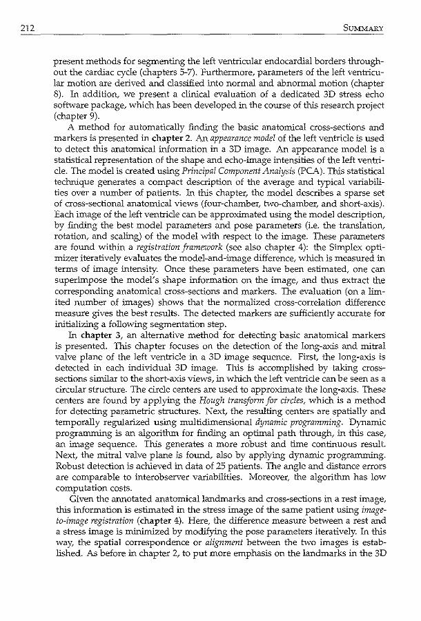
212 SuMMARY

present methods for segmenting the left ventricular endocardial borders through­out the cardiac cycle (chapters 5-7). Furthermore, parameters of the left ventricu­lar motion are derived and classified into normal and abnormal motion (chapter 8). In addition, we present a clinical evaluation of a dedicated 3D stress echo software package, which has been developed in the course of this research project (chapter 9).

A method for automatically finding the basic anatomical cross-sections and markers is presented in chapter 2. An appearance model of the left ventricle is used to detect this anatomical information in a 3D image. An appearance model is a statistical representation of the shape and echo-image intensities of the left ventri­cle. The model is created using Principal Component Analysis (PCA). This statistical technique generates a compact description of the average and typical variabili­ties over a number of patients. In this chapter, the model describes a sparse set of cross-sectional anatomical views (four-chamber, two-chamber, and short-axis). Each image of the left ventricle can be approximated using the model description, by finding the best model parameters and pose parameters (i.e. the translation, rotation, and scaling) of the model with respect to the image. These parameters are found within a registration frame--<»ork (see also chapter 4): the Simplex opti­mizer iteratively evaluates the model-and-image difference, which is measured in terms of image intensity. Once these parameters have been estimated, one can superimpose the model's shape information on the image, and thus extract the corresponding anatomical cross-sections and markers. The evaluation (on a lim­ited number of images) shows that the normalized cross-correlation difference measure gives the best results. The detected markers are sufficiently accurate for initializing a following segmentation step.

In chapter 3, an alternative method for detecting basic anatomical markers is presented. This chapter focuses on the detection of the long-axis and mitral valve plane of the left ventricle in a 3D image sequence. First, the long-axis is detected in each individual 3D image. This is accomplished by taking cross­sections similar to the short-axis views, in which the left ventricle can be seen as a circular structure. The circle centers are used to approximate the long-axis. These centers are found by applying the Hough transform for circles, which is a method for detecting parametric structures. Next, the resulting centers are spatially and temporally regularized using multidimensional dynamic programming. Dynamic programming is an algorithm for finding an optimal path through, in this case, an image sequence. This generates a more robust and time continuous result. Next, the mitral valve plane is found, also by applying dynamic programming. Robust detection is achieved in data of 25 patients. The angle and distance errors are comparable to interobserver variabilities. Moreover, the algorithm has low computation costs.

Given the annotated anatomical landmarks and cross-sections in a rest image, this information is estimated in the stress image of the same patient using image­to-image registration (chapter 4). Here, the difference measure between a rest and a stress image is minimized by modifying the pose parameters iteratively. In this way, the spatial correspondence or alignment between the two images is estab­lished. As before in chapter 2, to put more emphasis on the landmarks in the 3D

SUMMARY

image, only the sparse set of common anatomical views is used to calculate the difference measure. Qualitative and quantitative evaluation in 20 end-diastolic and 20 end-systolic images shows an improvement in alignment between rest and stress. Again, the normalized cross-correlation measure gives good results, close to the interobserver variabilities. Also, we demonstrate that the anatomical land­marks can be detected more robustly using this sparse distribution of anatomical views, rather than using the whole 3D image.

We now shift the focus from the initialization of anatomical markers to the detection of 3D endocardial borders of the left ventricle. In chapter 5, the active appearance model technique is applied for segmenting the 3D contours in an end­diastolic echocardiogram. The appearance model is generated as before; however, a full 3D model is used in this chapter. It is then matched to the image via re­gression techniques, which require prior training of the regression matrix. During each iteration, the pose and appearance parameters are updated linearly using the model-and-image difference and the regression matrix. The traditional matching method, which uses a fixed regression matrix, is compared with a new 'Jacobian tuning' method, which iteratively updates the regression matrix during match­ing. The latter leads to better accuracy and a larger capture range in the contour detection in 54 patient images.

Contour detection throughout the whole cardiac cycle is investigated in chap­ter 6. The contour in an end-diastolic 3D image is propagated (tracked) through­out the image sequence using spatial transforms, calculated with optical flow. This method estimates the motion of the myocardium via spatial and temporal im­age gradients. Naturally, this requires that the myocardium is visible in the im­age. However, this is not always the case for clinically acquired echocardiograms, since parts of the cardiac wall may be obscured due to suboptimal imaging con­ditions. So, to provide a time-continuous and physically plausible tracking result, a statistical model of cardiac motion is embedded in the optical flow method. In this way, the motion in regions where the cardiac wall is obscured is regularized by the motion of the visible cardiac wall. Good tracking results are obtained in 53 noncontrast image sequences and 27 contrast sequences, comparing well with results reported in literature. In good quality images, the combination of the pro­posed method with a basic optical flow algorithm (i.e. without statistical model) generates even better tracking results.

The contour detection method of chapter 6 is further improved using a proba­bilistic weight scheme, presented in chapter 7. Weights are derived by analyzing the temporal intensity profiles of the 3D image sequence using expectation maxi­mization (EM). In this chapter, a fast implementation of the EM method is used to estimate the probability that each image pixel corresponds with a 'station­ary', 'wandering', or 'lost' component in the probability density distribution. The derived weights reflect the probability that the cardiac wall is clearly visible or obscured by typical ultrasound artifacts. In areas where the cardiac wall is clearly visible, the motion is estimated using a basic optical flow method. In areas where the cardiac wall is obscured, the motion estimation relies on the statistical cardiac motion model. The quantitative assessment on 35 noncontrast sequences shows a further improvement in tracking accuracy, compared with the results of chapter

213

214 SUMMARY

6. To discriminate between normal and pathological cardiac wall motion, a clas­

sification method is proposed in chapter 8. Cardiac wall motion is represented by parameters of a statistical PCA model of the left ventricular shape, consisting of multiple cardiac phases. The orthomax rotation is applied to this PCA model, to generate a more compact representation of the wall motion in each left ventricular segment. This concise representation is achieved because the orthomax rotation generates more localized variations in spatial and temporal domains, whereas the traditional PCA model contains global variations. Wall motion classification using these statistical parameters is demonstrated in 129 two-dimensional echocardio­graphic sequences. Compared with the PCA model, the orthomax rotated repre­sentation attains a similar classification accuracy, but "With fewer parameters in a better-defined classification space.

In the course of this research project, a dedicated 3D stress echo software pack­age has been developed. This was necessary since this type of software had not been available commercially until very recently. In chapter 9, the first clinical evaluation of our software is presented. The essential functionality for analyz­ing 3D stress echo is investigated: side-by-side viewing of rest and stress data and the systematical selection and visualization of anatomical views. Two expert observers analyzed 34 noncontrast and contrast clinically available rest-stress im­ages visually. They compared the new software with traditional software which does not have this essential functionality. Using this new software, a drastic im­provement of interobserver agreement can be seen.

To conclude, we have come a long way in developing quantitative and ob­jective methods for analyzing 3D stress echo (chapter 10). Initialization, contour detection, and classification methods have been developed, which show that con­siderable advances have been made to allow a more robust and ac=ate analysis. We have also demonstrated the advantages of using dedicated software for the analysis of 3D stress echo in the clinical setting. Based on the research in this project, opportunities remain for further development, e.g. in the analysis of con­trast echocardiograms, enhancement of image quality, and improvement of clini­cal workflow. The tools developed within this research project can provide useful quantitative and objective parameters to help the clinical expert in the diagnosis of left ventricular function.

Samenvatting

Hart- en vaatziekten zijn een van de belangrijkste doodsoorzaken in de wester­se wereld. Het is daarom van groat klinisch belang om de tedmieken, die deze ziekten kunnen opsporen, te verbeteren. Stress echocardiografie (stress echo) is zo'n tedmiek. Het wordt vaak toegepast om verminderde functie van het hart­spierweefsel en het daarmee samenhangende coronairlijden te beoordelen. De methode werkt als volgt: de wandbeweging van het linkerventrikel wordt met echografie (beeldvorming via ultrageluid) zichtbaar gemaakt. Dit wordt gedaan als de patient in rust is en bij diverse niveaus van inspanning van de hartspier ( d.w.z stress). Aan de hand van deze beelden wordt de hartfunctie beoordeeld. Dit gebeurt normaliter visueel, wat kan leiden tot grate interpretatieverschillen tussen gebruikers.

Sinds kart is driedimensionale (3D) echografische beeldvorming beschikbaar. Deze afbeeldingstedmiek kan verschillende beperkingen van stress echo, die ge­woonlijk met tweedimensionale beeldvormlllg wordt uitgevoerd, voorkomen. Ten eerste kunnen de anatomische doorsneden in een 3D beeld achteraf exact geko­zen worden. Daamaast maakt deze tedmiek het mogelijk om de echte 3D wand­beweging te kwantificeren. In dit proefschrift presenteren we geautomatiseerde methoden om 3D stress echo objectief en kwantitatief te analyseren. Dit is beslist geen makkelijke taak, vanwege de !age spatiotemporele resolutie, de verschillen­de beeldartefacten, en de hoge snelheid waarmee de beelden dienen te worden geanalyseerd. In hoofdstuk 1 wordt de context van dit onderzoek geschetst, door een overzicht te geven van medische beeldvorming met ultrageluid, stress echo­cardiografie en methoden voor medische beeldverwerking. Ook worden het ter­rein en de doelen van het onderzoek in meer detail beschreven.

Om stress echo analyse te automatiseren, zijn een aantal verschillende rnetho­den ontwikkeld. Allereerst worden in hoofdstukken 2-4 technieken beschreven

216 SAc"'E:NVATTING

om anatornische pun ten (zoals de apex en rnitralisklep) in een beeld te vinden en om automatisch doorsneden te selecteren. Verder presenteren we methoden om het endocard van het linkerventrikel over de gehele hartcyclus te segmenteren (hoofdstukken 5-7). Vervolgens behandelen we de afleiding van bewegingspara­meters van het linkerventrikel, waarrnee onderscheid kan worden gemaakt tussen normale of abnorrnale wandbeweging (hoofdstuk 8). Daamaast presenteren we een klinische evaluatie van een computerprogramma dat speciaal gemaakt is voor 3D stress echo en ontwikkeld is in de loop van dit onderzoeksproject (hoofdstuk 9).

In hoofdstuk 2 wordt een methode gepresenteerd om de elementaire anatorni­sche punten en doorsneden in een 3D beeld te vinden. Om deze anatornische in­formatie te detecteren, wordt een zogenaamd appearance model van het linkerven­trikel gebruikt. Een appearance model is een statistische representatie van de vorm van het !inkerventrikel en de intensiteiten van het echobeeld. Dit model wordt gemaakt m.b.v. Principal Component Analysis (PCA). Deze statistische techniek ge­nereert een compacte beschrijving van het linkerventrikel, in termen van een ge­rniddelde en van de typische variabiliteit over een verzameling patienten. In wezen beschrijft het model in dit hoofdstuk slechts een selectie van anatornische vlakken (de vierkamer-, tweekamer-, en de korte-asdoorsneden). Elk beeld van een linkerventrikel kan worden benaderd m.b.v. deze modelbeschrijving, door de beste model- en orientatieparameters ( d.w.z. translatie, rota tie, en schaling) van het model ten opzichte van het beeld te vinden. Deze parameters worden be-­paald door registratie (zie ook hoofdstuk 4). Hiervoor gebruiken we het Simplex optimalisatiealgoritrne, dat het intensiteitsverschil tussen het beeld en het model minimaliseert. Zodra deze parameters zijn bepaald, kan de vorrninformatie van het linkerventrikelmodel worden toegepast op het beeld, en zodoende kunnen de anatornische doorsneden en punten worden geextraheerd. Uit de evaluatie ( op een beperkt aantal beelden) blijkt dat de genorrnaliseerde kruiscorrelatie als verschilmaat de beste resultaten geeft. De gedetecteerde anatornische pun ten zijn nauwkeurig genoeg voor een daaropvolgende segmentatiestap.

In hoofdstuk 3 wordt een altematief gepresenteerd om elementaire anato­rnische punten te detecteren. In dit hoofdstuk wordt de nadruk gelegd op de detectie van de lange as van het linkerventrikel en het vlak van de rnitralisklep in 3D beeldreeksen. Eerst wordt de lange as in elk afzonderlijk 3D beeld gevon­den. We gaan daarbij uit van transversale doorsneden, waarin het linkerventrikel als een cirkelvorrnige structuur te zien is. De rniddelpunten van deze cirkels be­naderen zo de lange as. Deze rniddelpunten worden gevonden door de Hough transformatie voor cirkels toe te passen, een methode om parametrische structuren te detecteren. Vervolgens worden de verkregen rniddelpunten in het spatiotempo­rele domein geregulariseerd m.b.v. multidimensionaal dynarnisch progranuneren (dynamic programming). Dynarnisch programmeren is een algoritrne om het opti­male pad te vinden door een netwerk van knooppunten (in dit geval, de pixels in een bee!dreeks). Deze aanpak !evert een betrouwbaar resultaat zonder spatiele en temporele onregelmatigheden. Daarna wordt het vlak van de rnitralisklep ge­detecteerd. Ook hiervoor gebruiken we dynarnisch programmeren. De methode !evert een goede detectie op in de beelden van 25 patienten. De hoek- en afstand-

SAMENVATTING

fout is vergelijkbaar met de variaties in het handmatig aangeven van de punten. Bovendien zijn de rekenkosten van het algoritme laag.

Als we de handmatig aangegeven anatomische punten en doorsneden in een rustbeeld hebben, kan deze informatie in een stress beeld van dezelfde patient worden bepaald met image-to-image registration (beeld-op-beeld registratie, hoofd­stuk 4). Deze methode minimaliseert het intensiteitsverschil tussen het rust- en het stressbeeld door iteratief (stapsgewijs) de orientatieparameters te veranderen. Op deze manier word! de spatiele uitlijning (alignment) tussen de twee beelden verkregen. Zoals oak in hoofdstuk 2 wordt er meer gewicht toegekend aan de anatomische punten in het 3D beeld, door slechts de selectie van standaard ana­tomische vlakken te nemen om het verschil te berekenen. De registratie methode laat een kwalitatieve en kwantitatieve verbetering zien in de uitlijning tussen rust en stress in 20 eind-diastolische en 20 eind-systolische beelden. Oak hier geeft de genormaliseerde kruiscorrelatiemaat goede resultaten, die de variabiliteit tussen twee gebruikers benaderen. Verder Iaten we zien dat de anatomische punten be­ter kunnen worden gedetecteerd met deze selectie van anatomische vlakken dan met het hele 3D beeld.

We verleggen nude aandacht van ir.itialisatie van anatomische punten en vlak­ken naar de detectie van het 3D endocardiale oppervlak van het linkerventrikel. In hoofdstuk 5 word! de active appearance model techniek gebruikt om 3D contou­ren in een eind-diastolisch echocarcliogram te segmenteren. In tegenstelling tot voorgaande hoofdstukken wordt in dit hoofdstuk een volledig 3D model gebruikt. Om een beeld te segmenteren word! het model met het beeld in overeenstemming gebracht (matching) via regressietechnieken. Dit vereist dat er vooraf een regres­siematrix is opgebouwd. Tijdens de matching worden de orientatie- en appearance parameters bij elke iteratiestap op lineaire wijze bijgesteld m.b.v. deze regressie­matrix en het verschil tussen model en beeld. De traditionele matching methode, waarbij een constante matrix word! gebruikt, wordt vergeleken met een nieuwe zogenaamde Jacobian tuning methode, die bij elke iteratie de regressiematrix bij­werkt. Uit de contourdetectie in 54 eind-diastolische patientbeelden blijkt dat deze nieuwe methode nauwkeuriger is en een groter convergentiebereik oplevert.

In hoofdstuk 6 word! contourdetectie over de gehele hartcyclus onderzocht. De contouren in een hele tijdreeks worden gevonden door spatiele transforma­ties uit te voeren tussen opeenvolgende beelden, uitgaande van de contouren in het eind-diastolische 3D beeld. Deze transformaties worden berekend met opti­cal flow. Met deze methode word! de beweging van de hartwand tussen twee opeenvolgende beelden bepaald, d.m.v. de spatiele en temporele gradienten. Dit vereist uiteraard dat de hartwand zichtbaar is in het beeld. Voor klinisch op­genomen echocardiogrammen is dit helaas niet altijd het geval, aangezien delen van de hartwand kunnen wegvallen door suboptimale beeldacquisitie. Daarom word! hier een statistisch model van de hartbeweging in de optical flow methode opgenomen, om een continue en fysiek plausibele segmentatie te verkrijgen. Op deze manier gebruiken we de beweging van de zichtbare hartwand als regulari­satie om de beweging te bepalen van gebieden waar de hartwand slecht te zien is. Deze nieuwe methode is getest op 53 tijdreeksen die zonder contrastrniddel zijn opgenomen en in 27 reeksen met contrast en !evert goede resultaten op. Bo-

217

218 SAMENVATTING

vendien steken de uitkomsten gunstig af tegen andere resultaten in de literatuur. In beelden van goede kwaliteit Ievert de combinatie van deze methode met een klassiek optical flow algoritme (zonder statistisch model) een verdere verbetering.

De contourdetectiemethode van hoofdstuk 6 wordt nog verder verbeterd met behulp van een probabilistische weging, die word! gepresenteerd in hoofdstuk 7. De wegingsfactoren worden afgeleid door de intensiteit-tijdsprofielen van de 3D reeks te analyseren met behulp van expectation maximization (EM). In d.it hoofd­stuk wordt een snelle irnplementatie van de EM methode gebruikt om voor elk beeldpixel de kans te bepalen dat het behoort tot een 'stationary', 'wandering', of 'lost' component in de kansverdeling. Op deze manier geven de afgeleide we­gingsfactoren aan of de hartwand goed zichtbaar is of dat die achter typische ultrageluidsartefacten schuil gaat. In gebieden waar de wand goed te zien is, wordt de beweging bepaald met de klassieke optical flow methode. In gebieden waar de wand slecht of niet zichtbaar is, wordt de beweging bepaald met het sta­tistisch hartbewegingsmodel. Dit laat een verdere kwantitatieve verbetering zien in 35 beeldreeksen zonder contrast, vergeleken met de resultaten van hoofdstuk 6.

De classificatiemethode in hoofdstuk 8 wordt gebruikt om onderscheid te rna­ken tussen normale en pathologische hartbeweging. Hier worden de parameters van een statistisch PCA model gebruikt om de hartwandbeweging te beschrijven. Dit model geeft de vorm van het linkerventrikel weer in verschillende hartfases. Vervolgens wordt de orthomax rotatie toegepast op dit PCA model. Dit resul­teert in een beknoptere representatie van wandbeweging in elk linkerventrikel­segment. De orthomax rota tie genereert namelijk meer gelokaliseerde varia ties in het spatiotemporele domein, terwijl het traditionele PCA model globale variaties beschrijft. Classificatie van wandbeweging met deze trad.itionele en orthomax pa­rameters is onderzocht in 129 twee-dirnensionale echocardiografische tijdreeksen. Met beide soorten parameters wordt een vergelijkbare classificatienauwkeurig­heid behaald. Echter, voor de orthomax methode zijn rninder parameters nodig. Bovend.ien is de classificatieruirnte beter gedefinieerd.

In de loop van dit onderzoeksproject is een speciaal 3D-stress echo software­pakket ontwikkeld, omdat er nog geen soortgelijk pakket comrnercieel beschik­baar was. In hoofdstuk 9 wordt de eerste klinische evaluatie van onze software gepresenteerd. De belangrijkste functionaliteit voor het analyseren van 3D stress echo wordt hler onderzocht, namelijk de weergave van rust en stress beelden naast elkaar en de systematische selectie en visualisatie van anatomische door­sneden. Twee experts voerden visuele analyses uit op klinisch verkregen rust- en stressbeelden van 34 patienten, met en zonder contrast. Hierbij werd zowel de nieuwe software getest als de traditionele software, die niet over deze belangrijk­ste functionaliteiten beschlkt. Door deze nieuwe software te gebruiken wordt de overeensternrning tussen de twee experts drastisch verbeterd.

We concluderen dat we aanzienlijke vooruitgang hebben geboekt in de ont­wikkeling van kwantitatieve en objectieve methoden voor het analyseren van 3D stress echo (hoofdstuk 10). We hebben initialisatie-, contourdetectie-, en classi­ficatiemethoden ontwikkeld, en aangetoond dat deze methoden de analyses be­trouwbaarder en nauwkeuriger maken. We hebben ook aangetoond dat het ge-

SAMENVATTING

bruik van speciale software voor de analyse van 3D stress echo waardevol is in de klinische omgeving. Naast de resultaten van dit onderzoek, resteert nog een aantal mogelijkheden voor verdere ontwikkeling, zoals bijvoorbeeld speciale me­thoden voor de analyse van contrast echobeelden, verbetering van beeldkwaliteit, en optimaliseren van het diagnostische proces in de klinische omgeving. De tech­nieken die ontwikkeld zijn binnen dit onderzoek kunnen nuttige, kwantitatieve en objectieve parameters opleveren. Deze bieden de klinische expert nieuwe mo­gelijkheden in het bepalen van de functie van het linkerventrikel.

219

Publications

Journal papers

Leung, K. Y. E., R. A Baldewsing_ F. Mastik, J. A Schaar, A Gisolf, and A F. W. van der Steen [2006]. Motion compensation for intravascular ultrasound palpography. IEEE Trans. Ultrason. Ferroelectr. Freq. ControL 53 (7). 1269-80.

Van Stralen, M., K. Y. E. Leung, M. M. Voonnolen, N. de Jong, A. F. W. van der Steen, J. H. C. Reiber, and J. G. Bosch [2008]. Tune continuous detection of fhe left ventricular long axis and fhe mitral valve plane in 3-D echocardiography. Ultrasound Med. BioL 34 (2). 196-207.

Leung_ K. Y. E., M. van Stralen, A Nemes, M. M. Voorrnolen, G. van Burken, M. L Ge­leijnse, F. J. ten Cate, J. H. C. Reiber, A F. W. van der Steen, N. de Jong, and J. G. Bosch [2008]. Sparse registration for fhree-dimensional stress echocardiography. IEEE Trans. Med. Imaging. 27 (11). 1568-79.

Leung, K. Y. E. and J. G. Bosch [2008]. Segmental wall motion classification in echocardio­grams using compact shape descriptors. Acad. Radio!. 15 (11). 1416-24.

Nemes, A, K. Y. E. Leung, G. van Burken, M. van Stralen, J. G. Bosch, 0. L L Soliman, B. J. Krenning, W. B. Vletter, F. J. ten Cate, and M. L Geleijnse [2009]. Side-by-side viewing of anatomically aligned left ventricular segments in three-dimensional stress echocardiography. Echocardiography. 26 (2). 189-95.

Leung_ K. Y. E., M. G. Danilouchkine, M. van Stralen, N. de Jong, A F. W. van der Steen, and J. G. Bosch [2009a ]. Motion-guided optical flow tracking for segmenting 4D echocardiograms, submitted.

222 PUBLICATIONS

Leung, K. Y. E., M.G. Danilouchkme, M. van Stralen, N. de Jong, A. F. W. van der Steen, and J. G. Bosch [2009b]. Probabilistic framework for improving tracking in artifact­prone 3D echocardiograms, submitted.

Peer-reviewed conference proceedings

Leung, K. Y. E., M. van Stralen, G. van Burken, M. M. Voormolen, A. Nemes, F. J. ten Cate, N. de Jong, A. F. W. van der Steen, J. H. C. Reiber, and J. G. Bosch [2006]. Sparse appearance model based registration of 3D ultrasound images. Proc. Med. Imaging Augment. Real. LNCS 4091. 236-43.

Leung, K. Y. E. and J. G. Bosch [2007a]. Local wall-motion classification in echocardiograms using shape models and orthomax rotations. Proc. Funct. Imaging Model. Heart. LNCS 4466. 1-11.

Leung, K. Y. E. and J. G. Bosch [2007b]. Localized shape variations for classifying wall motion in echocardiograms. Proc. Med. Image Cornput. Comput. Assist. Interv. LNCS 4791. 52-9.

Other conference proceedings

Leung, K. Y. E., R. A. Baldewsing, F. Mastik, M.G. Danilouchkme, J. A. Schaar, A. Gisolf, and A. F. W. van der Steen [2005a}. Motion compensation for intravascular ultrasound palpography for in vivo vulnerable plaque detection. Proc. Int. Con£. Ultrason. Meas. Imaging Tissue Elasticity. 67.

Leung, K. Y. E., R. A. Baldewsing, F. Mastik, J. A. Schaar, A. Gisolf, and A. F. W. van der Steen [2005b ]. Motion compensation for intravascular ultrasound palpography for in vivo vulnerable plaque detection. Proc. IEEE Int. Ultrason. Symp. 209-10.

Leung, K. Y. E., M. van Stralen, M. M. Voormolen, G. van Burken, A. Nemes, F. J. ten Cate, M. L. Geleijnse, N. de Jong, A. F. W. van der Steen, J. H. C. Reiber, and J. G. Bosch [2006a]. Registration of 2D cardiac images to real-time 3D ultrasound volumes for 3D stress echocardiography. Proc. SPIE Med. Imaging. 6144. 614418.

Leung, K. Y. E., M. van Stralen, G. van Burken, M. M. Voormolen, A. Nemes, F. J. ten Cate, M. L. Geleijnse, N. de Jong, A. F. W. van der Steen, J. H. C. Reiber, and J. G. Bosch [2006b ]. Sparse appearance model based registration and segmentation of 3D echocardiographic images. Proc. IEEE Int. Ultrason. Symp. 2413-6.

Van Stralen, M., K. Y. E. Leung, M. M. Voormolen, N. de Jong, A. F. W. van der Steen, J. H. C. Reiber, and J. G. Bosch [2007a]. Automatic segmentation of the left ventricle in 3D echocardiography using active appearance models. Proc. IEEE Int. Ultrason. Symp. 1480-3.

Van Stralen, M., K. Y. E. Leung, M. M. Voormolen, N. de Jong, A. F. W. van der Steen, J. H. C. Reiber, and J. G. Bosch [2007b]. Fully automatic detection of left ventricular long

PuBLICATIONS

axis and mitral valve plane in 3D echocardiography. Proc. IEEE Int. u1trason. Symp. 1488-91.

Leung, K. Y. E., M. van Stralen, M. M. voormolen, N. de Jong, A. F. W. van der Steen, J. H. C Reiber, and J. G. Bosch [2008]. Improving 3D active appearance model segmentation of the left ventricle with jacobian tuning. Proc. SPIE Med. Imaging. 6914. 69143B.

Leung, K. Y. E., M. G. Danilouchkine, M. van Stralen, N. de Jong, A. F. W. van der Steen, and J. G. Bosch [2009]. Tracking left ventricular borders in 3D echocardiographic se­quences using motion-guided optical flow. Proc. SPIE Med. Imaging. 7259. 72590W.

Abstracts

Leung, K. Y. E., R. A. Baldewsing, F. Mastik, J. A. Schaar, A. Gisolf, and A. F. W. van der Steen [2005]. Motion compensation for intravascular ultrasound palpography for in vivo vulnerable plaque detection. In: IEEE Int. Ultrason. Symp. Rotterdam, The Nether­lands, IC -4, 209.

Leung, K. Y. E., M. van Stralen, M. M. Voormolen, G. van Burken, A. Nemes, F. J. ten Cate, M. L. Geleijnse, N. de Jong, A. F. W. van der Steen, J. H. C Reiber, and J. G. Bosch [2006a]. Registration of 2D cardiac images to real-time 3D ultrasound volumes for 3D stress echocardiography. In: SPIE Med. Imaging. San Diego, CA., 6144--44, 160.

Leun& K. Y. E., M. van Stralen, G. van Burken, M. M. Voormolen, A. Nemes, F. }. ten Cate, M. L. Geleijnse, N. de Jong, A. F. W. van der Steen, J. H. C Reiber, and J. G. Bosch [2006b]. Sparse appearance model based registration and segmentation of 3D ultrasound images. In: IEEE Int. Ultrason. Symp. Vancouver, Canada, PS-8/45, 32.

Bosch, J. G., M. van Stralen, K. Y. E. Leung, M. M. Voormolen, N. de Jong, and A. F. W. van der Steen [2007]. Quantification of left ventricular volume and endocardial wall motion in real-time 3D echocardiography. In: First Dutch Conference on Bio-Medical Engineering. Egmond aan Zee, The Netherlands, 140.

Vander Steen, A. F. W., J. A. Schaar, F. Mastik, C. L. de Korte, K. Y. E. Leung, A. Gisolf, and P. W. J. C. Serruys [2007]. Intravascular ultrasound palpography for vulnerable plaque detection. In: First Dutch Conference on Bio-Medical Engineering. Egmond aan Zee, The Netherlands, 173.

Leung, K. Y. E., M. van Stralen, M. M. Voormolen, N. de Jong, A. F. W. van der Steen, J. H. C Reiber, and J. G. Bosch [2008a]. Improving 3D active appearance model seg­mentation of the left ventricle with jacobian tuning. In: SPIE Med. Imaging. San Diego, CA., 6914-122,62.

Nemes, A., K. Y. E. Leung, G. van Burken, M. van Stralen, J. G. Bosch, 0. I. I. Soliman, B. J. Krenning, W. B. Vletter, F. J. ten Cate, and M. L. Geleijnse [2008]. Side-by-side viewing of anatomically aligned left ventricular segments in three-dimensional stress echocardiography. In: ESC Congress, Eur. HeartJ. Vol. 29. Miinchen, Germany, 279-80.

Leung, K. Y. E., A. Nemes, G. van Burken, M. van Stralen, J. G. Bosch, 0. I. I. Soliman, B. J. Krenning, W. B. Vletter, F. J. ten Cate, and M. L. Geleijnse [2008b]. Improving in­terobserver agreement of three-dimensional stress echocardiography using novel side­by-side viewing software. In: Euroecho. Lyon, France, 1178, S160.

223

224 PUBLICATIONS

Leung, K. Y. E., M.G. Danilouchkine, M. van Stralen, N. de Jong, A. F. W. van der Steen, and J. G. Bosch [2009]. Tracking left ventricular borders in 3D echocardiographic se­quences using motion-guided optical flow. In: SPIE Med. !mag. Orlando, FL., 7259-31, 60.

Acknowledgments

This thesis describes the research performed at the Biomedical Engineering group, Thoraxcenter, Erasmus MC, the Netherlands. Contrary to what the cover sug­gests, this PhD thesis is certainly not a one-woman effort. The assistance pro­vided by many people has proved to be invaluable, so I will gladly take the time to acknowledge them.

First of all, I would like to thank my promotors Prof. van der Steen and Prof. de Jong. Ton, thanks for keeping a bird's eye view of my research. Your enthusiasm and vision on research cooperations have been very inspiring. Nico, thank you for showing much interest in my research. Your questions, although often difficult to answer, always motivate me to think ahead.

Dr. Hans Bosch, somehow you always manage to find time for our weekly meetings. Thank you for your innovative ideas and your always constructive comments. I hope the quality of this thesis does justice to your supervision.

I would also like to thank the other members of my doctoral committee, Prof. Wiro Niessen, Prof. Hans Reiber, Dr. Folkert ten Cate, Prof. Alison Noble, Dr. Chris de Korte, and Prof. Maarten Simoons, for their time and effort in reading this thesis. Thank you for being a member of the doctoral committee.

Also, thanks to all my (past and present) colleagues on the 23rd floor for the moments of sanity in the 'fish tank'. Marijn, many chapters in this thesis would not have been realized without you. Your determination and optimism have been a source of inspiration. Thanks for proofreading chapter 10. Marco, thanks for letting me play with the FRU, and for your no-nonsense view on the list of authors. Gerard, thank you for realizing 3DStress View. Thanks for taking a practical approach to the many software and hardware issues I have had. Mike, thanks for your willingness to correct my never-ending manuscripts. Your skills

226 ACKNOWLEDGMENTS

and experience in image processing have been invaluable. Thanks for proofread­ing chapters 1 and 4. Dr. Dr. Johannes, thanks for your sense of humor and for your support. Frits, thanks for your useful comments and the great supervision when I was working on palpography. Thanks for proofreading chapter 2. Mar­cia and Klazina, thanks for being such good roommates during conferences and courses. Marcia, thanks for proofreading chapter 3. Sandra, thank you for your kindness, dating back to the time at the TU. Thanks for proofreading chapter 5. Paul, thank you for being such a great boxing' partner. Thanks for proofreading chapter 6. Egon, thank you for setting a great example by graduating before me. Thanks for proofreading chapter 7. Rik, thank you for always being helpful and patient, even during my early 'practicum' days. Thanks for proofreading chap­ter 8. Robert, thank you for the interesting conversations about almost anything. Thank you for your help with the cover design, and for proofreading chapter 9. Margreet, thank you for your company during the frequent rides to work and home, and for teaching me new things in MATLAB. Thanks for proofreading the summary. Thomas, thanks for your courage in exploring an unfamiliar research direction. Thanks to Annemieke, Jolanda, Fokko, Frank, Gijs and Lambert for your excellent efforts in innovative research. Hans Verdoes, thanks for putting your computer expertise to good use (especially when I had given up hope on recovering data ... ). Mieke, Monique, and Marianne, our secretaries, thank you for your assistance in preparing many documents over the past few years. Mieke, thanks for your help with the Dutch abstract. Thanks also to all other colleagues: Alina, Antoinette, Ayache, Cees, Charles, Dave, David, Dol£, Geert, Guillaume, Hans S., Harald, Jan, Jerome, Kim, Prof. Klaas Born, Krista, Lambert, Leo, Mar­tijn, Miranda, Mirza, Peggy. Radj, Richard, Riekje, Telli, Toshihiko, and Wim, for creating such a welcoming and enthusiastic environment for research.

I would like to acknowledge our clinical experts at the Thoraxcenter. Without you, we would have no data to work with. Dr. ten Cate, thank you for enabling the nice cooperation between the clinic and our technical department. Dr. At­tila Nemes, thank you for putting up with experimental software at the start of this project. Dr. Osama Soliman, thanks for your interest in 3DStressView and your experience in contour delineation. Dr. Boudewijn Krenning, thanks for ac­quiring FRU data using prototype hardware ('press Ctrl+F8 to save'). Dr. Marcel Geleijnse, thank you for your realistic and practical view on stress echo. Wun Vletter, thank you for making the perfect echo images with which to test our algorithms.

Furthermore, many thanks to the LKEB group at Leiden University Medical Center. Prof. Reiber, thank you for enabling the nice cooperation between Lei­den and Rotterdam. Dr. Boudewijn Lelieveldt, thank you for your encouraging remarks and useful ideas. Meng Ma, thanks for working on the 3D stress echo project together and for realizing the ASM ideas. I would also like to thank all researchers at the Biomedical Imaging Group Rotterdam at the Erasmus MC, the Image Sciences Institute at the UMC Utrecht, the Clinical Physics Laboratory at UMC St Radboud, and the Physics of Fluids group in Twente for the nice time during the conferences and courses.

To all JOVOs: thanks for the 'gezelligheid' and your enthusiasm; keep up the

ACKNOWLEDGMENTS

good work! I would also like to thank Els, Rosalinde, Armemarie, Christel, and Henk for the much needed musical diversion in the weekend.

Pa and ma, Bo and Eugene, grandmas and grandpas: thank you for your love, support, and encouragement. Thank you for reminding me of the important things in life. Hans and Joke, Ruth and Patrick, Sam and Ludy, Hanna and Bert, Joelle, opa & oma van der Zwan and Ottenhoff, thank you for receiving me with open arms in your family.

Timo, I am truly grateful for your love. Your sense of humor and your ability to put things into perspective have been very refreshing. Life would be much less fun without you. I hope that we may continue to share many happy moments together.

Finally, the most important person I would like to thank is my Lord and savior Jesus Christ. "Oh, the depth of the riches both of the wisdom and knowledge of God! How unsearchable are His judgments and His ways past finding out!".

Esther Leung

2009

22.7

Curriculum vitae

K. Y. Esther Leung was born in Hong Kong on August 18, 1981. She obtained her VWO degree at the Sondervick College in Veldhoven, the Netherlands, in 1999. 1n 2005, she received her master's degree in Applied Physics (cum laude) from the Delft University of Technology. During her internship at the Netherlands Organization for Applied Scientific Research (TNO), she investigated clustering algorithms for seabed sediment discrimination. The subject of her master thesis was motion compensation for intravascular ultrasound strain imaging. Currently, she is pursuing her Ph.D. degree at the department of Biomedical Engineering (Thoraxcenter, Erasmus MC, Rotterdam, the Netherlands) on the subject of three­dimensional stress echocardiography. Her research interests include medical ul­trasound, image processing, and clinical applications development.

PhD portfolio summary

PhD Student: PhD period:

K. Y. E. Leung 2005-2009

Erasmus MC department: Research school:

Biomedical Engineering, Thoraxcenter COEUR

Promotors: Prof. dr. ir. A.F.W. van der Steen Prof. dr. ir. N. de J ong

Supervisor: dr. ir. J.G. Bosch

Activity Location General academic SJ....:ills

Biomedical English -writing and commu- Rotterdam nicat:ion (Erasmus MC) Classical methods for data analysis (Ni- Rotterdam hes)

In-depth courses Pathophysiology of ischemic heart dis- Rotterdam ease (COEUR) Cardiovascular imaging and diagnostics Rotterdam (COEUR) Knowledge driven image segmentation Lei den (ASCI) Medical imaging: principles, ultrasounds Archamps & magnetic resonance (ESMP) Advanced pattern recogrition (ASCI) Delft European course on 3D echocardiogra- Rotterdam phy (Erasmus MC)

Seminars and workshops Ultrasound contrast agents - theory and Rotterdam experimental methods (IEEE)

Year

2006

2007

2005

2005

2005

2006

2006 2006

2005

ECTS

4.0

5.7

1.5

1.5

1.5

1.5

1.5 0.4

0.1

Continued on next page

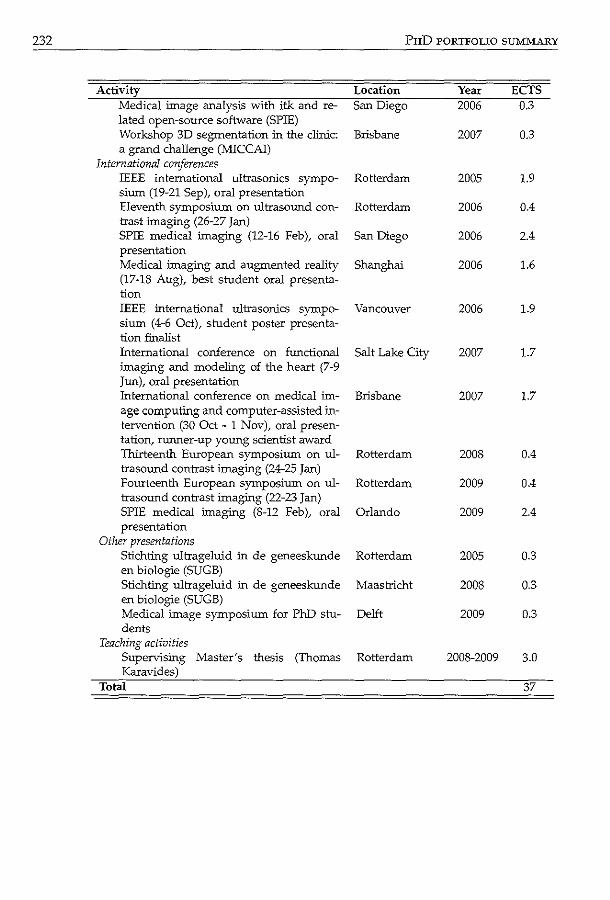
232 PHD PORTFOLIO SUMMARY

Activity Medical image analysis with itk and re­lated open-source software (SPIE) Workshop 3D segmentation in the clinic: a grand challenge (MICCAI)

International conferences IEEE international ultrasonics sympo­sium (19-21 Sep), oral presentation Eleventh symposium on ultrasound con­trast imaging (26-27 Jan) SPIE medical imaging (12-16 Feb), oral presentation Medical imaging and augmented reality (17-18 Aug), best student oral presenta­tion IEEE international ultrasonics sympo­sium (4-6 Oct), student poster presenta­tion finalist International conference on functional imaging and modeling of the heart (7-9 Jun), oral presentation International conference on medical im­age computing and computer-assisted in­tervention (30 Oct- 1 Nov), oral presen-tation, runner-up young scientist award Thirteenth European symposium on ul­trasound contrast imaging (24-25 Jan) Fourteenth European symposium on ul­trasound contrast imaging (22-23 Jan) SPIE medical imaging (8-12 Feb), oral presentation

Other presentations Stichting ultrageluid in de geneeskunde en biologie (SUGB) Stichting ultrageluid in de geneeskunde en biologie (SUGB) Medical image symposium for PhD stu­dents

Teaching activities

Location San Diego

Brisbane

Rotterdam

Rotterdam

San Diego

Shanghai

Vancouver

Salt Lake City

Brisbane

Rotterdam

Rotterdam

Orlando

Rotterdam

Maastricht

Delft

Superv:isiDg Master's thesis (Thomas Rotterdam Karavides)

Total

Year ECTS 2006 0.3

2007 0.3

2005 1.9

2006 0.4

2006 2.4

2006 1.6

2006 1.9

2007 1.7

2007 1.7

2008 0.4

2009 0.4

2009 2.4

2005 0.3

2008 0.3

2009 0.3

2008-2009 3.0

37