


Aspects of SupergravityCompactifications and SCFT
correlators
Amin Ahmad Nizami
Hughes Hall
Department of Applied Mathematics and Theoretical Physics,
Faculty of Mathematics,
University of Cambridge
This dissertation is submitted for the degree of Doctor of Philosophy.
February 2014
Abstract
We begin by discussing aspects of supergravity compactifications and argue
that the problem of finding lower-dimensional de Sitter solutions to the classi-
cal field equations of higher-dimensional supergravity necessarily requires under-
standing the back-reaction of whatever localized objects source the bulk fields.
However, we also find that most of the details of the back-reacted solutions are
not important for determining the lower-dimensional curvature. We find, in par-
ticular, a classically exact expression that, for a broad class of geometries, directly
relates the curvature of the lower-dimensional geometry to asymptotic properties
of various bulk fields near the sources. The near-source profile of the bulk fields
thus suffices to determine the classical cosmological constant. We find that, due to
the existence of a classical scaling symmetry, the on-shell supergravity action for
IIA, IIB and 11d supergravity theories is a boundary term whose explicit form we
also determine. Specializing to codimension-two sources, we find that the contri-
bution involving the asymptotic behaviour of the warp factor is precisely canceled
by the contribution of the sources themselves. As an application we show that
all classical compactifications of Type IIB supergravity (and F-theory) to 8 di-
mensions are 8D-flat if they involve only the metric and the axio-dilaton sourced
by codimension-two sources, extending earlier results to include warped solutions
and more general source properties. We then proceed to study 3d SCFTs in the
superspace formalism and discuss superfields and on-shell higher spin current mul-
tiplets in free 3d SCFTs. For N = 1 3d SCFTs we determine the superconformal
invariants in superspace needed for constructing 3-point functions of higher spin
operators, find the non-linear relations between the invariants and consequently
write down all the independent invariant structures, both parity even and odd,
for various 3-point functions of higher spin operators. We consider the additional
constraints of higher spin current conservation on the structure of 3-point func-
tions and show that the 3-point function of higher spin conserved currents is the
sum of two terms- a parity even part generated by free SCFTs and a parity odd
part.
Declaration
The research described in this dissertation was carried out in the Department
of Applied Mathematics and Theoretical Physics at the University of Cambridge
between May 2010 and December 2013. Chapters 3 and 4 include work which
was done, in part, at the Tata Institute of Fundamental Research, Mumbai, India
during a research visit (August 2012 - March 2013). Except where reference is
made to the work of others, all the results are original and based on the following
of my works:
• Superspace formulation and correlation functions of 3d superconformal field
theories, Amin A. Nizami, Tarun Sharma and V. Umesh, arXiv:1308.4778
[hep-th].
• On Brane Back-Reaction and de Sitter Solutions in Higher-Dimensional Su-
pergravity, C.P. Burgess, A. Maharana, L. Van Nierop, Amin A. Nizami, F.
Quevedo, JHEP 1204 (2012) 018, arXiv:1109.0532 [hep-th].
None of the work contained in this dissertation has been submitted by me for
any other degree, diploma or similar qualification.
Signed
(Amin Ahmad Nizami)
Date
2

Acknowledgements
I thank Fernando Quevedo for all his help and support and for hosting me at
ICTP, Trieste for the many visits during the first year of my PhD. I thank Shiraz
Minwalla for hosting me during an extended visit (August 2012 - March 2013) at
TIFR, Mumbai, India.
I am grateful to the Cambridge Commonwealth Trust for continued finan-
cial support. I also thank the Abdus Salam International Centre for Theoretical
Physics, Trieste, Italy for financial support during the first two years of my PhD.
I thank Trinity College, Cambridge for a Rouse Ball Travelling Studentship and
the Lundgren fund for fourth year support.
I wish to thank Hugh Osborn and Carlos Nunez for agreeing to be examiners
for the PhD viva and for pointing out errors and inaccuracies in the thesis. I would
like to thank all the people with whom I have learned many things in numerous
conversations: H. Osborn, J. H. Park, S. Minwalla, S. Raju, R. Loganayagam,
V. Umesh, T. Sharma, C. Burgess, A. Maharana, D. Dorigoni, J. Hofmann, A.
Rudra, P. Zhao.
I am grateful to my family, especially my mother and brother, and all my
friends, here in Cambridge and in India, for their support.
Above all, I wish to record my gratitude to God.
3

Contents
1 Introduction 5
1.1 Supergravity and de Sitter spacetime . . . . . . . . . . . . . . . . 6
1.2 Higher spin operators in CFTs . . . . . . . . . . . . . . . . . . . . 12
1.3 Holographic interpretations . . . . . . . . . . . . . . . . . . . . . 18
2 Supergravity compactifications and dS no-go theorems 21
2.1 No-go results and the 6D loophole . . . . . . . . . . . . . . . . . . 23
2.2 Constraints on scalar curvature of X due to that of Y . . . . . . . 25
2.3 A general expression for the classical cosmological constant . . . . 29
2.4 Scaling in Supergravity . . . . . . . . . . . . . . . . . . . . . . . . 33
2.4.1 Scaling and the on-shell action . . . . . . . . . . . . . . . . 34
2.4.2 11 dimensional Supergravity . . . . . . . . . . . . . . . . . 35
2.4.3 IIA Supergravity . . . . . . . . . . . . . . . . . . . . . . . 35
2.4.4 IIB Supergravity . . . . . . . . . . . . . . . . . . . . . . . 37
2.5 Sources and singularities . . . . . . . . . . . . . . . . . . . . . . . 39
2.6 Example: the axio-dilaton IIB supergravity . . . . . . . . . . . . . 45
2.6.1 Bulk equations of motion . . . . . . . . . . . . . . . . . . . 46
2.6.2 Flat unwarped solutions . . . . . . . . . . . . . . . . . . . 47
2.6.3 Warped solutions . . . . . . . . . . . . . . . . . . . . . . . 48
2.6.4 Near-source Kasner solutions . . . . . . . . . . . . . . . . 50
3 Superspace formulation of SCFTs with higher spin operators 56
3.1 Superspace . . . . . . . . . . . . . . . . . . . . . . . . . . . . . . . 57
3.2 Free SCFTs in superspace and conserved higher spin currents . . 61
3.2.1 General structure of the current superfield . . . . . . . . . 61
4
3.2.2 Free field construction of currents . . . . . . . . . . . . . . 63
3.3 Weakly broken conservation . . . . . . . . . . . . . . . . . . . . . 68
4 3-point functions of higher spin operators 75
4.1 Two-point functions . . . . . . . . . . . . . . . . . . . . . . . . . 76
4.2 Three-point functions . . . . . . . . . . . . . . . . . . . . . . . . . 78
4.2.1 Superconformal invariants for 3-point functions of N = 1
higher spin operators . . . . . . . . . . . . . . . . . . . . . 78
4.2.2 Relations between the invariant structures . . . . . . . . . 83
4.2.3 Simple examples of three point functions . . . . . . . . . . 86
5 Summary and Outlook 92
5

Chapter 1
Introduction
The AdS/CFT correspondence [20, 21, 22] provides a duality map between large
N Superconformal Field Theories (SCFTs) and supergravity theories in higher di-
mensions. Certain large N SCFTs, for example, 4d N = 4 Super Yang-Mills and
3d N = 6 ABJ theory have a holographic dual description in terms of supergrav-
ity compactification geometries - IIB supergravity on the background geometry
AdS5 × S5 [20] or IIA supergravity on AdS4 × CP3 [28], respectively. In this
thesis we will first study certain aspects of supergravity compactifications mainly
pertaining to the maximally symmetric spacetime obtained on warped compact-
ification. We will investigate, in particular, the feasibility of generating de Sitter
solutions. We will also discuss a (classical) scaling symmetry possessed by the
IIA, IIB and 11d supergravity theories and the on-shell action of these theories,
consequently, being a boundary term. We will study the effects of codimension
2 brane sources on the lower dimensional curvature. Next we turn to the study
of 3d SCFTs. We first discuss the superspace formalism for studying these theo-
ries, and in particular the construction of conserved higher spin currents in free
3d SCFTs. We then investigate the structure of 3-point functions of higher spin
operators and the constraints of current conservation, extending earlier work of
[35].
In this introductory chapter we will briefly review some underlying basic no-
tions which should be useful for the later chapters.
6
1.1 Supergravity and de Sitter spacetime
Supergravity theories are supersymmetric theories where the global supersymme-
try group is gauged. In this case the supersymmetry transformations depend on
parameters which are (locally) space-time dependent. Such theories are theories
of gravity where the graviton, described by the metric gµν has a supersymmetric
counterpart- the gravitino (ψµα). The actions of such theories, in varying number
of dimensions, were constructed in the 1970’s and provide a supersymmetric ex-
tension of the Einstein-Hilbert action by including terms corresponding to various
bosonic/fermionic fields in the supergravity multiplet. We will be interested in the
following basic supergravity theories from which most other supergravity theories
(in lower dimensions) are naturally obtained by dimensional reduction.
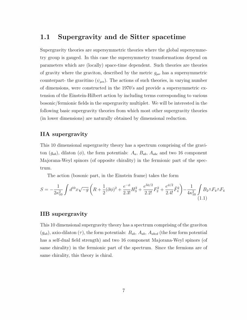
IIA supergravity
This 10 dimensional supergravity theory has a spectrum comprising of the gravi-
ton (gab), dilaton (φ), the form potentials: Aa, Bab, Aabc and two 16 component
Majorana-Weyl spinors (of opposite chirality) in the fermionic part of the spec-
trum.
The action (bosonic part, in the Einstein frame) takes the form
S = − 1
2κ210
∫d10x√−g(R +
1
2(∂φ)2 +
e−φ
2.3!H2
3 +e3φ/2
2.2!F 2
2 +eφ/2
2.4!F 2
4
)− 1
4κ210
∫B2∧F4∧F4
(1.1)
IIB supergravity
This 10 dimensional supergravity theory has a spectrum comprising of the graviton
(gab), axio-dilaton (τ), the form potentials: Bab, Aab, Aabcd (the four form potential
has a self-dual field strength) and two 16 component Majorana-Weyl spinors (of
same chirality) in the fermionic part of the spectrum. Since the fermions are of
same chirality, this theory is chiral.
7
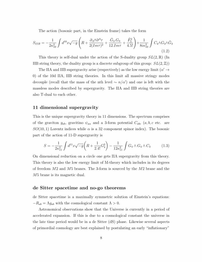
The action (bosonic part, in the Einstein frame) takes the form
SIIB = − 1
2κ210
∫d10x√−g
(R +
∂Aτ ∂Aτ
2(Imτ)2+
G3.G3
12.Imτ+F 2
5
4.5!
)+
1
8iκ210
∫C4∧G3∧G3
(1.2)
This theory is self-dual under the action of the S-duality group SL(2,R) (In
IIB string theory, the duality group is a discrete subgroup of this group: SL(2,Z))
The IIA and IIB supergravity arise (respectively) as the low energy limit (α′ →0) of the 10d IIA, IIB string theories. In this limit all massive stringy modes
decouple (recall that the mass of the nth level ∼ n/α′) and one is left with the
massless modes described by supergravity. The IIA and IIB string theories are
also T-dual to each other.
11 dimensional supergravity
This is the unique supergravity theory in 11 dimensions. The spectrum comprises
of the graviton gab, gravitino ψaα and a 3-form potential Cabc (a, b, c etc. are
SO(10, 1) Lorentz indices while α is a 32 component spinor index). The bosonic
part of the action of 11-D supergravity is
S = − 1
2κ211
∫d11x√−g(R +
1
2.4!G2
4
)− 1
12κ211
∫G4 ∧G4 ∧ C3 (1.3)
On dimensional reduction on a circle one gets IIA supergravity from this theory.
This theory is also the low energy limit of M-theory which includes in its degrees
of freedom M2 and M5 branes. The 3-form is sourced by the M2 brane and the
M5 brane is its magnetic dual.
de Sitter spacetime and no-go theorems
de Sitter spacetime is a maximally symmetric solution of Einstein’s equations:
−Rab = Λgab with the cosmological constant Λ > 0.
Astronomical observations show that the Universe is currently in a period of
accelerated expansion. If this is due to a cosmological constant the universe in
the late time period would be in a de Sitter (dS) phase. Likewise several aspects
of primordial cosmology are best explained by postulating an early “inflationary”
8
phase of rapid accelerated expansion of the universe so that its early time be-
haviour was also dS to a fair degree of accuracy. This gives an added significance
to understanding physics in de Sitter backgrounds. There are several aspects of
de Sitter spacetime which are ill-understood. It possesses a cosmological event
horizon and an associated temperature and entropy [1] which are hard to under-
stand from a microscopic perspective. The Hilbert space of quantum gravity in
de Sitter (dS) has been argued to be of finite dimension [2,3,4], a claim which is
seemingly at variance with a proposed dS/CFT correspondence [5,6]. At a more
basic level it is of interest to determine whether, in higher dimensional theories
like supergravity and string theory, compactifications to de Sitter spacetime can
be naturally obtained.
Kaluza-Klein compactifications of supergravity theories were extensively stud-
ied in the 70’s and 80’s with phenomenological applications in mind, and the par-
ticle spectrum and resultant possible compactified geometries investigated. There
are no-go theorems, which we discuss and review next, which show that, under
certain assumptions, such compactifications can not be realised as solutions of
higher dimensional supergravity theories. The no-go result is that time inde-
pendent compactifications of supergravity theories on compact manifolds with no
singularities can’t result in dS. Thus cosmological models of early (inflationary)
and late (cosmological constant dominated) universe can not be based on such
theories. As is usual with no-go theorems, it may be the case that altering the
assumptions which go into the proof can potentially alter the conclusion. In par-
ticular, we aim to explore the effect of singular sources such as backreacting branes
on the lower dimensional scalar curvature. Though we are not able to generate
new dS solutions, we do extend the no-go theorems.
No-go Theorems on de Sitter compactifications in Super-
gravity
We consider warped compactifications in supergravity theories where the D di-
mensional spacetime is a warped product: MD = Xd ×w YD−d of a maximally
symmetric d dimensional spacetime (Xd) and a compact D− d dimensional space
9

(YD−d). The most general D dimensional line element that is consistent with d
dimensional Poincare invariance is
ds2 = gMN(x)dxMdxN = gµν(x, y)dxµdxν + gmn(y)dymdyn
= e2W (y)gµν(x)dxµdxν + gmn(y)dymdyn (1.4)
(W (y) is the warp factor) 1. We have the relations
Rµν = Rµν +e(2−d)Wgµν
d∇2edW (1.5)
Rmn = Rmn + d[∇m∇nW + (∇mW )(∇nW )] (1.6)
A simple no-go theorem [7] now follows if we take the compact manifold Y to
have no boundaries (in particular no singular brane sources). It is known that the
bosonic energy momentum tensor of all conventional supergravity theories obeys
the Strong Energy Condition:
−RMNvMvN =
(TMN −
gMN
D − 2T
)vMvN ≥ 0 (1.7)
for all timelike or null vectors vM . In particular for v timelike and ∼ (1, 0, 0, ....)
we get
−R00 = −R00 +e(2−d)W
d∇2edW ≥ 0 (1.8)
Now Xd is maximally symmetric so Rµν = Rd
dgµν . Multiplying the above equation
by e(d−2)W√g and integrating over Y gives:
Rd
dVW +
1
d
∫Y
dD−dy√g∇2edW ≥ 0 (1.9)
1notation and convention: indices M,N = 0, 1, . . . , D−1 run over all dimensions and give the
coordinates onMD; greek indices µ, ν = 0, 1, . . . , d−1 denote lower-dimensional coordinates(on
Xd); and indices m,n = 1, . . . , n = D − d denote compactified coordinates (on YD−d). We
use RMN to denote the D-dimensional Ricci curvature of the full D-dimensional metric, gMN ;
and Rµν to denote the d-dimensional Ricci curvature computed from the d-dimensional metric,
gµν = e2W gµν . Also, gD = det gMN while gd = det gµν etc.. Also we use a ‘mostly plus’ metric
and Weinberg’s curvature conventions [55], which differ from those of MTW [56] only in the
overall sign of the definition of the Riemann tensor. This means that it is the scalar curvature
−R that would be positive for dS and negative for AdS.
10
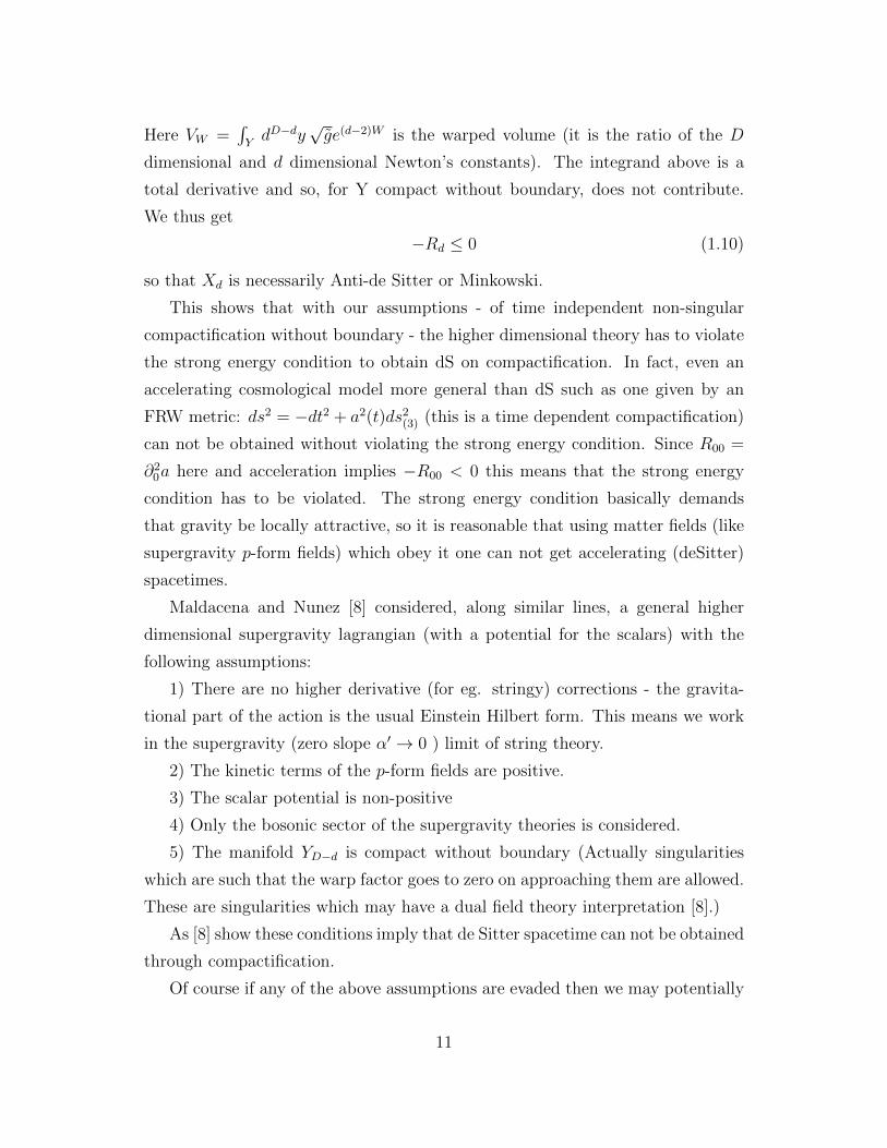
Here VW =∫YdD−dy
√ge(d−2)W is the warped volume (it is the ratio of the D
dimensional and d dimensional Newton’s constants). The integrand above is a
total derivative and so, for Y compact without boundary, does not contribute.
We thus get
−Rd ≤ 0 (1.10)
so that Xd is necessarily Anti-de Sitter or Minkowski.
This shows that with our assumptions - of time independent non-singular
compactification without boundary - the higher dimensional theory has to violate
the strong energy condition to obtain dS on compactification. In fact, even an
accelerating cosmological model more general than dS such as one given by an
FRW metric: ds2 = −dt2 + a2(t)ds2(3) (this is a time dependent compactification)
can not be obtained without violating the strong energy condition. Since R00 =
∂20a here and acceleration implies −R00 < 0 this means that the strong energy
condition has to be violated. The strong energy condition basically demands
that gravity be locally attractive, so it is reasonable that using matter fields (like
supergravity p-form fields) which obey it one can not get accelerating (deSitter)
spacetimes.
Maldacena and Nunez [8] considered, along similar lines, a general higher
dimensional supergravity lagrangian (with a potential for the scalars) with the
following assumptions:
1) There are no higher derivative (for eg. stringy) corrections - the gravita-
tional part of the action is the usual Einstein Hilbert form. This means we work
in the supergravity (zero slope α′ → 0 ) limit of string theory.
2) The kinetic terms of the p-form fields are positive.
3) The scalar potential is non-positive
4) Only the bosonic sector of the supergravity theories is considered.
5) The manifold YD−d is compact without boundary (Actually singularities
which are such that the warp factor goes to zero on approaching them are allowed.
These are singularities which may have a dual field theory interpretation [8].)
As [8] show these conditions imply that de Sitter spacetime can not be obtained
through compactification.
Of course if any of the above assumptions are evaded then we may potentially
11
realise positive curvature solutions. Although one may like to have a de Sitter
realisation within a fully non-perturbative (finite α′ and gs) string/M theoretic
framework it is typically quite hard to go much beyond assumption 1 and we
will here not attempt to work beyond the supergravity regime. Assumption 2
seems quite reasonable though it is violated in Hull’s II*A,B theories (obtained
by T-dualising IIB,A on a timelike circle) where de Sitter compactifications (for
eg. dS5×H5 in II*B, H being the hyperbolic space) are possible [9], see also [10].
However these theories seem to be ill-defined because of the negative sign kinetic
term for the R−R fields.
Assumption 3 would be violated, for example, if we start with a supergravity
theory in higher dimensions with a positive cosmological constant. In 6d gauged
supergravity with a positive (exponential) potential explicit 4d dS solutions have
been constructed [14]. Typically we would expect a potential only to be generated
through compactification and we will take the higher dimensional theory to be
without an arbitrary potential.
It is to be noted that the strong energy condition is a quite strong one and
violated by physically realistic systems (unlike, for example, the null energy con-
dition). By incorporating fermions and thus coupling the theory to matter this
condition can be violated. We will however take assumption 4 to hold.
The manifold YD−d being compact implies the lower dimensional Newton’s
constant (Gd) is finite. If one consider Y to be non-compact, in particular hyper-
bolic, then it is possible to get de Sitter solutions. In such a case, however, it is
not clear how to obtain a discrete d dimensional spectrum. We willl take Y to be
compact but allow it to have boundaries (thus partially evading assumption 5).
In particular, we willl consider the boundaries to be singularities (of a type more
general than allowed in 5) in the compact manifold Y due to the presence of brane
sources. It may be noted that in the above no-go theorems the p-form field poten-
tials which contribute to TMN are included but the (p − 1)-branes which source
these fields are considered to be probe branes with negligible effect on the ambient
geometry. We may, however, wish to include the effects of brane backreaction.
We also keep ourselves to considering only time-independent compactifications.
Note that the above theorems need not hold if we consider Y to be Lorentzian
12
and X a maximally symmetric space- such an accelerating cosmology would be a
time-dependent compactification[10,11]. From the viewpoint the lower (d) dimen-
sional observer this would give rise to time-dependent scalar (moduli) fields. In
this case one considers more general time dependent compactifications along the
lines of [15,16,17]. These authors discuss the constraints on realising accelerating
cosmologies from higher dimensional compactifications. Considering two deriva-
tive higher dimensional theories compactified on a manifold without boundary
which is flat (in the sense of having zero Ricci curvature scalar) or is conformally
flat, they show that obtaining accelerating cosmologies requires violations of the
null energy condition. More precisely, for an FRW cosmology with equation of
state parameter w the null energy condition requires that there exists a thresh-
old value wth (which depends on the number of compact dimensions) such that
−1 ≤ w ≤ wth and for which the number of e-foldings is bounded from the above
(also this number goes to zero as w → −1 and thus dS can not be realised). Thus,
only transient acceleration can be obtained, as also shown earlier in [10], and in
particular we can not have a dark energy due to a cosmological constant only.
The maximum number of e-foldings possible is also too small to get a realistic
description inflation. We note however that if we consider the compact manifold
to have singularities or if it is not Ricci flat or conformally Ricci flat then realizing
cosmic acceleration may not require violations of the null energy condition.
1.2 Higher spin operators in CFTs
Conformal Field Theories (CFTs) are of prime importance in theoretical physics
for several reasons. They are important in the study of phase transitions as
various statistical mechanical systems at criticality are described by CFTs. This
historically was the principal reason for their introduction and motivation for their
study. They describe fixed points of renormalization group flows and general
QFTs can be defined and studied through deformations of CFTs by marginal
operators. Through the AdS/CFT duality they map holographically to higher
dimensional quantum theories of gravity and thus provide a non-perturbative
construction of such theories. We give below, a brief overview of some well known
13

basic CFT concepts.
The symmetry group of a CFT (the Conformal Group) is SO(D, 2) in D space-
time dimensions (D ≥ 3). All fields transform in representations of SO(D, 2).
Representations are labelled by Cartans of the maximal compact subgroup SO(D)×SO(2) : R and dimension ∆. In particular, for the 3 dimensional case we will
be dealing with, the conformal group is SO(3, 2) (isomorphic to OSp(2,R)) with
representations being labelled by ∆ and the SO(3) spin s. For 3d SCFTs with
N extended supersymmetry, the supergroup of superconformal symmetries is
OSp(2,R|N ) which has the maximal compact bosonic subgroup SO(2)×SO(3)×SO(N ) with the associated Cartan charges labelling the representations: (∆, s, hi),
hi being the SO(N ) Cartan charges (SO(N ) is the R-symmetry group).
CFT Definition (usual): One considers local fields transforming in a repre-
sentation R and the Action (more generally, Path Integral) invariant under this
transformation on the field variables. This is a perturbative definition- the usual
way QFTs are defined, about weakly coupled saddle points of the path integral.
For CFTs it is possible to give a non-perturbative definition by giving the
spectrum of all local primary operators together with the Wilson coefficients
[O∆,R, cijk]. Indeed many CFTs do not have any lagrangian description. This
includes the (2,0) SCFT which is central to M-theory and describes M5 brane
dynamics, and many other N = 2 4d SCFTs (of the so-called S class) which can
be obtained from the compactification of the (2,0) theory on a Riemann surface
with punctures.
The CFT spectrum comprises of local primary operators O∆ ([Kµ, O∆] = 0)
with scaling dimension ∆; and representationR of SO(D) in which O∆ transforms
(and the R-charges for an SCFT). All the local operators are in a one to one cor-
respondence with states in the radial quantization scheme via the state-operator
map.
The dynamical content of a CFT is encoded in the Wilson coefficients via the
Operator Product Expansion:
Oi(x)Oj(0) =∑k
cijkF (x, ∂y)Ok(y) |y=0 (1.11)
The OPE is an exact operator relation (with a finite radius of convergence) in any
14
CFT, unlike the usual case in QFTs where it is an asymptotic expansion.
Unitarity imposes additional constraints on the spectrum in terms of lower
bounds on the dimensions of primaries: ∆ ≥ ∆min(R)
Conformal symmetry is quite constraining. It fixes the form of the 2 and 3
point functions of scalar conformal primary operators. The form of the 2-point
function is:
〈φ∆(x1)φ∆(x2)〉 =k
x2∆12
(1.12)
and we may normalise to set k = 1.
With the 2-point function normalised, the 3-point function is also completely
fixed upto an overall constant
〈φ∆1(x1)φ∆2(x2)φ∆3(x3)〉 =c123
x2α12312 x2α231
23 x2α31231
(1.13)
with αijk =∆i+∆j−∆k
2
The overall constant c123 - a three point coupling, is not arbitrary but encodes
dynamical information about the theory.
The spectrum together with the Wilson coefficients comprise the CFT data
and its knowledge completely specifies the CFT. This is because the OPE can in
principle be used recursively to reduce an n-point function of local primary oper-
ators to a sum of products of 2-point functions with various derivative operations.
The Wilson coefficients being known, this expression is completely determined.
Furthermore, since any descendent is determined by the action of some number
of derivatives on a primary, it follows that the the n-point functions of all local
operators are completely known.
However the operator dimensions and Wilson coefficients are not arbitrary real
numbers. Apart from the constraints of unitarity they are constrained by OPE
associativity (also called crossing symmetry) seen at the level of 4-point functions.
4-point functions are not fixed by conformal symmetry on kinematic grounds but
their functional form is quite constrained.
15
〈φ∆(x1)φ∆(x2)φ∆(x3)φ∆(x4)〉 =1
x2∆12 x
2∆34
f(u, v) (1.14)
where u, v are the conformal cross-ratios:
u =x2
12x234
x213x
224
v =x2
14x223
x213x
224
(1.15)
The function f can be expanded in terms of conformal blocks
f(u, v) =∑O
cOgO(u, v) (1.16)
The sum is over all the primaries in the spectrum and the conformal block -
gO(u, v) encodes the contribution of the exchange of O within the 4-point function
and all its conformal descendents.
Crossing symmetry (OPE associativity) states that one can do OPE contrac-
tion of different operators within the correlation function- and different ways
should give same results. This leads to further constraints on f in the form
of the bootstrap equation:
v∆f(u, v) = u∆f(v, u) (1.17)
The basic idea of the bootstrap approach to QFTs is to use general principles
like Symmetries, Unitarity, Analyticity, to determine physical observables of inter-
est which may be S matrices. In CFTs one uses unitarity and crossing symmetry
to constrain the correlators. Note that since u, v can take arbitrary real values,
and the function f can be expanded using the OPE in terms of products of OPE
coefficients (the conformal block expansion of the 4-point function), the above
bootstrap equation in effect gives an infinite number of equations in infinitely
many variables (OPE coefficients and operator dimensions). In general there is
no way known to solve them but in special cases, for example 2d CFTs where the
finite dimensional SO(2, 2) is in fact extended to the infinite dimensional Virasoro
group one can find an explicit solution- these are the well known Minimal Model
solutions of 2d CFTs with central charge c < 1 [23]
For CFTs with higher spin operators, the 2-point function is again completely
fixed by conformal symmetry
16
〈Os,∆(1)Os,∆(2)〉 =unique tensor structure
x2∆12
(1.18)
The 3-point function is determined as a sum of a finite number of tensor
structures with undetermined constant coefficients
〈Os1,∆1(1)Os2,∆2(2)Os3,∆3(3)〉 =finitely many tensor structures
x2α12312 x2α231
23 x2α31231
(1.19)
The 4-point functions of higher spin primary operators have not been ex-
tensively investigated (other than some work on spin 1 and spin 2 four-point
functions).
In this thesis we will be dealing with superconformal field theories (SCFTs).
These are special CFTs which additionally also have supersymmetry. Apart from
the generators of the conformal group, the symmetry generators in this case in-
clude the supersymmetry generators (Qaα) and the generators of special super-
conformal transformations (Saα). The differential form of the action of all the
symmetry generators in superspace (for 3d SCFTs) is given by eq. (3.1) in Chap-
ter 3 and the full superconformal algebra is given by eq. (3.56) in an appendix to
that chapter.
Superconformal symmetry provides additional constraints on the field theory.
Superconformal representations are classified by superconformal primaries - these
are lowest weight states annhilated by Saα (besides Kµ). The raising operator here
is Qaα (like Pµ in the conformal case). Due to the nilpotent nature of the action of
Q’s, the superconformal multiplets are necessarily finite-dimensional and a single
representation of the superconformal algebra headed by a superconformal primary
contains within it many conformal primaries (its Q descendants), and hence many
conformal representations. We will discuss in greater detail in Chapters 3 and 4,
SCFTs in three dimensions and particularly their superspace formulation and
correlators of higher spin operators.
17
Significance of higher spin operators and the Maldacena-
Zhiboedov theorem
It is expected that CFTs which have any additional higher spin symmtery, and
corresponding conserved higher spin currents, would be free. This is analogous
to the Coleman-Mandula theorem for Poincare symmetry. In 3 dimensions it was
proven recently by Maldacena and Zhiboedov [31]. Under the assumptions of a
unique spin 2 conserved current and finitely many degrees of freedom (finite N)
for the CFT they showed, using lightcone OPE methods, that the existence of
a single higher spin (s > 2) current suffices to demonstrate the existence of an
infinite tower of higher spin currents. Furthermore n-point correlators of such
conserved higher spin currents factorise into products of 2-point functions which
signals that the theory is free.
In chapter 3 we formulate superspace methods for studying free 3d SCFTs and
construct explicitly the higher spin currents that these theories have in terms of
free superfields.
In subsequent work [32] QFTs with exact conformal symmtry but weakly bro-
ken higher spin symmtery (1/N corrections being the source of symmetry break-
ing) were considered. Such theories are interacting- indeed a plethora of examples
is known starting from the basic O(N) vector model and including various super-
conformal Chern-Simons theories like ABJ theory. At large N, there is a weakly
broken higher spin symmetry with an anomalous ”conservation” law
∂ · J(s) =1
NJ(s1)J(s2) + higher trace terms if possible (1.20)
Here s > 2 (the energy-momentum tensor is always exactly conserved). This
controlled breaking of higher spin symmetry in large N vector models can be used
to further constrain correlators of these interacting CFTs as demonstrated in [32]
The Virasoro Algebra provides an infinite dimensional extension of the Confor-
mal Algebra in two dimensions and enables the implementation of the conformal
bootstrap - the 2d Minimal Model exact solutions [23]. In higher dimensions, Vi-
rasoro symmetry is lacking. However, it appears from recent work [31], [32] that
higher spin symmetry might play an analogous role. The difference is that while 2d
18
CFTs with exact Virasoro symmetry can be non-trivial, in d > 2 CFTs with exact
higher spin symmetry are free, as shown in [31]. However, as mentioned above,
CFTs can have a parametrically small weakly-broken higher symmetry, and this
provides further constraints. This was seen at the level of 3-point functions in [32]
but the same analysis is expected to work for higher correlators. It may thus be
feasible that judicious use of (weakly broken) higher spin symmetry can be used
for the conformal bootstrap (at least for large N) of higher dimensional CFTs.
1.3 Holographic interpretations
As is well known, the AdS/CFT correspondence [20] states that conformal quan-
tum field theories can be holographically dual to certain quantum gravity theories
in AdS backgrounds in higher dimensions. In particular, 4d N = 4 super Yang-
Mills theory is holographically dual to IIB string theory on AdS5×S5 and the 3d
N = 6 ABJ superconformal Chern-Simons theory is dual to IIA string theory on
AdS4 ×CP3. This is a strong-weak coupling duality, and in general the tractable
domain is where the bulk/boundary theory is weakly coupled. In particular the
strongly coupled large N , large λ limit of a CFT is well described by an AdS bulk
geometry where the effective gravitational dynamics is that of Einstein gravity.
In this limit, the equivalence ZCFT = ZQG between partition functions becomes
ZCFT [J ] = exp(−Sos+∫J.φ), which is the well-known GKPW prescription [22, 21]
for computing correlators of strongly coupled CFTs (Sos is the on-shell action).
This is the most extensively studied corner of the AdS/CFT duality.
It is of interest to determine what kinds of CFTs admit holographic duals with
a geometric description. In other words, under what conditions is the dynamics
of the CFT encoded in a metric based semi-classical description of a gravitational
theory. This has been investigated [33, 34] and it is known that such a bulk geo-
metric interpretation exists whenever there is a large parameter in the CFT such
that the dimensions of a few (low spin) primary operators (the single-trace pri-
mary operators) do not become parametrically large as N →∞. This ’gap’ in the
spectrum, i.e, the existence of a level of low dimension primary operators ensures
a dual geometric description in terms of an effective semi-classical gravitational
19

description. 1/N corrections in the field theory amount to quantum corrections
in the bulk theory.
In CFTs where there are infinitely many higher spin single-trace primary op-
erators of minimal twist (τ = ∆−s) we do not expect the holographic duals to be
classical bulk geometries described by the Einstein-Hilbert action, since Einstein
gravity contains a unique spin two massless graviton and no higher spin massless
particles.
Higher spin bulk theories and CFTs with higher spin oper-
ators
The holographic duals to CFTs with a tower of higher spin operators are theories of
interacting higher spin massless fields in AdS. Although such theories do not exist
in flat space-time (as demonstrated by no-go theorems proved by Weinberg [46]),
the presence of a cosmological constant (dS/AdS spacetime) allows interacting
massless higher spin theories to exist. The existence of such theories can also be
inferred from string theory. In the usual infinite tension (α′ → 0 , T ∼ 1/α′ →∞)
supergravity limit of string theory, all massive stringy modes decouple (recall
that the mass of the nth level ∼ n/α′) and one is left with the massless modes
whose dynamics is described by supergravity. The opposite limit, the tensionless
limit, is when the AdS curvature scale is much smaller than the string length
(R/ls 1, which is the same as α′ → ∞). In this limit all the massive levels
become massless and one expects a complicated interacting theory of infintely
many massless modes which captures the dynamics of string theory in the extreme
stringy regime. Vasiliev has constructed a non-linear theory of interacting massless
higher spin fields in AdS [39] and this construction is expected to be the tensionless
limit of classical string theory (though this has not been demonstrated yet).
It was conjectured by Klebanov and Polyakov [24] that the bosonic O(N)
vector model (a 3d CFT) is dual to Vasiliev (type A) theory. When the singlet
scalar in the theory has mimimal dimensionality ∆ = 1 we have a free bosonic
CFT whereas for ∆ = 2 the theory is the critical O(N) model (obtained by
RG flow, from the free CFT to the Wilson-Fisher fixed point, triggered by the
20
relevant deformation (φ.φ)2). Similarily the type B Vasiliev theory is dual to
the fermionic O(N) vector model [25] - for ∆ = 2 we have the free fermion
CFT whereas for ∆ = 1 the critical theory - the Gross-Neveu model. Thus
these 3d CFTs are dual to higher spin theories (with even integer spin fields)
where the boundary conditions (on the boundary of AdS) preserve the higher spin
symmetry. It is also possible to choose boundary conditions which (weakly) break
the higher spin symmetry (at O(1/N) by multi-trace terms) and such theories have
as boundary duals interacting 3d CFTs which are Chern-Simons gauge theories
with bosons/fermions transforming in the fundamental (vector) representation of
the gauge group. Examples include the U(N) Chern-Simons theories studied in
[26], [27]. Although supersymmetry is not an essential ingredient of the vector
model/ higher spin duality one can indeed consider supersymmetric versions of
Vasiliev’s theory which would have superconformal field theories as duals [30, 29].
Although we will not explicitly discuss these theories in great detail in this thesis,
the material presented in Chapters 3 and 4 - regarding the superspace formalism,
higher spin operators and correlation functions - is of much revelance to their
study.
21

Chapter 2
Supergravity compactifications
and dS no-go theorems
de Sitter space, or slow-roll geometries close to de Sitter space, appear to play an
important role in cosmology. This has motivated searching for explicit solutions to
the higher-dimensional field equations for which the large four dimensions we see
are de Sitter or de Sitter-like. Although a few such solutions are known [47, 48],
more and more general no-go results [49, 50, 51, 52] show that such solutions are
difficult to find1 It is interesting to enquire about the reasons for this.
In this chapter we argue that part of the problem is that we are not yet using all
of the ingredients that de Sitter solutions may require. In particular, contributions
have been neglected that are the same size as some of the contributions that are
usually kept when searching for (or ruling out) de Sitter-like solutions.
The neglected contributions come from the actions of any localized sources
that may be present in the extra-dimensional configurations of interest. In par-
ticular, we argue here that for codimension-two sources these actions contribute
to the curvature an amount that is competitive with the contribution of the bulk
fields, including their back-reaction. In particular, the source action acts to sys-
tematically cancel the contribution from the warping of the noncompact geometry
1Four-dimensional effective field theories of string theory including non-perturbative effects
and anti branes or D-terms [53] can give rise to de Sitter solutions. But at the moment there is no
full understanding from the microscopic higher-dimensional theory. For other recent attempts
for de Sitter solutions see [54].
22

across the extra dimensions. This is important because the sign of the warping
contribution is usually definite, and because it is opposite to what is required for
a de Sitter noncompact geometry it plays a role in the various extant de Sitter
no-go results.
We study the effects of brane backreaction, source properties and bulk singu-
larities on obtaining de Sitter compactifications in higher dimensional supergravity
theories. We show how the lower dimensional scalar curvature (the cosmological
constant) is determined by the on-shell bulk action, warping effects, source action
and space-filling fluxes and is, in certain quite general cases, a sum over boundary
terms and thus determined by the asymptotic form of the bulk fields in the near-
brane limit. As an application we show that all codimension 2 brane solutions
(warped or unwarped) in axio-dilaton-metric theories are flat.
This chapter is organised as follows. We first discuss the no-go theorems
on de Sitter compactifications proved in the introduction. We then show how,
in warped compactifications, the curvature of the compact manifold constrains
the curvarure of the non-compact maximally symmetric part. In section 2.3 we
establish our main result: a general expression that relates the lower dimensional
scalar curvature to the on-shell bulk action of a theory and also includes effects
due to warping, source action and any space-filling fluxes which might be present.
In order to be able to put this relationship to use we show, in section 2.4, how the
on-shell action of a theory with a classical scaling symmetry is just a boundary
contribution. We show that the actions of 11-D supergravity, IIA, IIB supergravity
(respectively) have this scaling behaviour and we explicitly evaluate the on-shell
action as a sum over boundary contributions.
As an application we consider on-brane geometries for codimension 2 brane
sources. Explicit analytical expressions for unwarped D7 brane solutions in IIB
supergravity (axio-metric-dilaton sector) are known and are 8 dimensional flat.
We show that even after incorporporating the effects of warping and source effects
the solutions are still flat, thus generalising the result.
23

2.1 No-go results and the 6D loophole
Our interest is in D-dimensional metrics of the form
ds2 = gMN dxMdxN = e2W (y) gµν(x) dxµdxν + gmn(y) dymdyn , (2.1)
where D = d + n; the d-dimensional metric, gµν , is maximally symmetric (i.e.
flat, de Sitter or anti-de Sitter); and the warp factor, W , can depend on position
in the n compact directions (whose metric, gmn, is so far arbitrary).
In particular, for cosmological applications there is much interest in identifying
solutions to higher-dimensional field equations for which gµν is a de Sitter metric
(which in our curvature conventions 2 satisfies R = gµνRµν < 0). The search for
such solutions has been fairly barren, and this is partly explained by refs. [49], [50],
[51] and [52], who identify increasingly general obstacles to finding this type of de
Sitter solution to sensible, higher-dimensional, second-derivative field equations.
On the other hand, a handful of explicit solutions of this type do exist, includ-
ing 4D de Sitter solutions [47] for six-dimensional Maxwell-Einstein systems,
SME = −∫
d6x√−g
1
2κ2gMNRMN +
1
4FMNFMN + Λ
, (2.2)
with positive 6D cosmological constant, Λ. Similar solutions [48] also exist for
six-dimensional gauged, chiral supergravity [57], whose relevant bosonic action is
Sbulk = −∫
d6x√−g
1
2κ2gMN
(RMN + ∂Mφ ∂Nφ
)+
1
4e−φFMNFMN +
2 g2R
κ4eφ.
(2.3)
For both of these actions RMN denotes the Ricci tensor for the 6D metric, gMN ,
and F = dA is the field strength for a 6D gauge potential, AM . The quantity
κ2 = 8πG6 denotes the 6D gravitational coupling, while for the supersymmetric
case gR denotes the gauge coupling of a specific UR(1) gauge group that does not
commute with 6D supersymmetry.
These examples do not contradict the various no-go theorems because they
arise in systems which do not satisfy one of the assumptions of each. For instance,
2We use a ‘mostly plus’ metric and Weinberg’s curvature conventions [55], which differ from
those of MTW [56] only in the overall sign of the definition of the Riemann tensor.
24

the no-go result of [50] assumes that any extra-dimensional scalar potential must
be negative (as it tends to be for higher-dimensional supergravities, but is not so
for eqs. (2.2) and (2.3)). They evade the less restrictive assumptions of [51] and
[52], some of which exclude [52] having only two extra dimensions, n = 2. More
importantly they do not satisfy the average ‘boundedness’ assumptions [51] that
exclude solutions that are too singular.
The potential relevance of back-reaction
There are two ways to view the possibility that singular behaviour can suffice to
evade the no-go results. One view is to regard solutions with such singularities
as unacceptable, and so draws the conclusion that de Sitter solutions may be
impossible to find. And for some types of singularity (like negative-mass black
holes) this is probably right, since the alternative requires admitting energies that
are unbounded from below.
But some (apparent) singularities are known to be perfectly sensible, such
as those seen in Coulomb’s law at the position of a source charge. In the case
of Coulomb’s law, the singularity doesn’t preclude taking the solution seriously
because we don’t intend to trust the solution in any case right down to zero size.
The existence of apparent singularities might similarly be expected to arise in
the gravitational theories relevant to cosmology, provided these are regarded as
effective descriptions of some more-microscopic degrees of freedom. One can hope
to get a handle on deciding whether a singularity might be reasonable for an
effective description, by seeing what kinds of apparent singularities actually can
emerge from localized sources governed by physically reasonable actions.
These considerations suggest that understanding the back-reaction of localized
sources could be a crucial part of obtaining de Sitter solutions, or ruling them
out. In particular the asymptotics, and apparent divergence, of bulk fields near
a source is likely to be important, and is ultimately controlled by the action that
describes the dynamics of that source. Notice for these purposes ‘source’ need not
mean a fundamental object, like a D-brane. Rather, it could describe something
more complicated, like a soliton or a higher-dimensional brane wrapping internal
dimensions or a localized but strongly warped region. All we need know is that
25
the sources are much smaller than the extra dimensions within which they sit.
How the properties of a source affect the properties of bulk fields is best
understood at present for codimension-one and codimension-two sources. For
codimension-one sources, the back-reaction is described by the Israel junction
conditions [58], as is familiar from Randall-Sundrum models [59]. But bulk fields
with codimension-one sources also tend not to diverge at the source positions, and
so shed little light on how such singularities influence the low-energy curvature.
It is only for higher-codimension sources that it is generic that bulk fields diverge
at the source positions, and so where the relation between bulk singularity and
source properties can be explored.
Of course, these bulk singularities make matching bulk solutions to source
properties more complicated, usually requiring a renormalization of the source
[60]. The tools for detailed bulk-source matching and renormalization are most
explicitly known for codimension-two objects [61, 62, 63, 64, 65]. In particu-
lar, these tools have recently been used to identify [66] explicit objects that can
source the de Sitter solutions [48] of the 6D supergravity action, eq. (2.3). Since
the required source properties seem physically reasonable,3 they show that the
singularities in the corresponding bulk solutions need not be regarded as grounds
for their rejection.
2.2 Constraints on scalar curvature of X due to
that of Y
We discuss here how the scalar curvature of X (the non-compact maximally sym-
metric d-dimensional spacetime) is constrained by that of Y (the compact D − ddimensional manifold) if we require X to be dS. In [12] it was noted that the scalar
curvature (−Rd) of X gets a positive contribution from a negative scalar curva-
ture (−RD−d) of Y . We’ll derive here a simple relationship between Rd, RD−d
(≡ gmnRmn) and Td (≡ gµνTµν - the d dimensional trace of the energy momentum
3As discussed in more detail below, their worst feature appears to be a requirement that
the dilaton, φ, grows as one asymptotically approaches the sources, and so care must be taken
to avoid leaving the weak-coupling regime before reaching the source.
26

tensor) for a manifold MD = Xd ×w YD−d with total energy-momentum tensor
TMN
We will use equations (1.5) and (1.6). The D dimensional Einstein equation
is 4
−RMN = TMN −gMN
D − 2TD (2.4)
Consider first the d dimensional (µν) components of this equation. Since
gµν ≡ gµν = e2Wgµν we have
−Rµν = Tµν −e2WgµνD − 2
TD (2.5)
Now using eq. (1.5) and that
TD ≡ gMNTMN = gµνTµν + gmnTmn = e−2WTd + TD−d (2.6)
(Here gmn = gmn and TD−d ≡ gmnTmn) we get
−Rµν −e(2−d)Wgµν
d∇2edW = Tµν −
e2WgµνD − 2
(e−2WTd + TD−d)
Contracting the above equation with gµν gives
−Rd =D − d− 2
D − 2Td −
de2W
D − 2TD−d + e(2−d)W ∇2edW (2.7)
Likewise, we consider the D − d dimensional (mn) components of eq. (2.4)
−Rmn = Tmn −gmnD − 2
TD (2.8)
Now contracting equation (1.6) with gmn and simplifying gives
gmnRmn = RD−d + d∇2eW
eW(2.9)
so eq. (2.8) upon contraction and using the above equation leads to
−RD−d =d− 2
D − 2TD−d −
D − dD − 2
e−2WTd + d∇2eW
eW(2.10)
Eliminating TD−d between eqs. (2.7) and (2.10) gives us
−Rd = − 2
d− 2Td +
de2W
d− 2RD−d + e(2−d)W ∇2edW +
d2
d− 2eW ∇2eW (2.11)
4Here TD is the D dimensional trace of the energy-momentum tensor: TD ≡ gMNTMN .
27

Now multiplying the above equation by√ged−2W and integrating over YD−d
gives us the desired relation:
−RdVW = − 2
d− 2
∫dD−dy
√ge(d−2)WTd +
d
d− 2
∫dD−dy
√gedWRD−d (2.12)
+
∫dD−dy
√g∇2edW +
d2
d− 2
∫dD−dy
√ge(d−1)W ∇2eW
We note that for d > 2 the contribution of a negative Td and negative −RD−d
to −Rd is positive. In the case of no warping (W = 0), d = 4 and D = 10 , so that
we are considering 4 dimensional compactifications of 10 dimensional supergravity
theories the above relation reduces to eq. (1.1) of [13]:
−R4 = −T4 + 2R6 (2.13)
Thus even if some kind of energy condition enforces the positivity of Td, it may
be possible to compensate for this by having compact manifolds with scalar curva-
ture everywhere negative thus leading to positive curvature for the d-dimensional
space-time. Many compactications are known with X a Minkowski or AdS space-
time and Y a manifold with non-negative scalar curvature. For example, AdS5×S5
in IIB string theory, AdS4×S7 in 11D supergravity (here Y has positive scalar cur-
vature) andM4×CY3 in heterotic string theory (here Y- the Calabi-Yau manifold-
is Ricci flat and so the scalar curvature is zero). However, it seems quite difficult
to realise compactifications with Y having negative scalar curvature. Finding any
such solutions would help in realising de Sitter compactifications.
Summary of results
We examine how source back-reaction constrains the existence of de Sitter solu-
tions in more general higher-dimensional theories than the six-dimensional ones
already explored.
In particular, we explore some of these issues in eleven-dimensional supergrav-
ity, and in ten-dimensional Type IIB and Type IIA supergravity. Because our
best-developed tools apply to codimension-two objects, it is these we largely ex-
plore in detail. If only D-branes were allowed as sources, this would restrict us to
28

D7-branes in Type IIB systems. But we also explore the other supergravities for
two reasons: because some of our results apply equally well to higher-codimension
sources; and because our sources might not be D-branes — or (p, q) branes for that
matter — but instead be more complicated localized codimension-two quantities
(like very small warped throats).
We find the following results:
• First, for geometries of the form of eq. (2.1), we find a very general classical
relationship that gives the curvature in the non-compact dimensions parallel
to the sources as the sum of four terms: R ∝ I + II + III + IV , where IV
vanishes for maximally symmetric geometries in the absence of space-filling
fluxes.
• Second, we show that contribution I — which is proportional to the bulk
action evaluated at the classical back-reacted solution — is very generally
given as the integral of a total derivative, and so is controlled by the bound-
ary values of a particular combination of bulk fields. This property relies
only on the existence of a classical scale invariance that is shared by most
higher-dimensional supergravities (and holds in particular for 11D and 10D
Type IIA and IIB supergravity).
• Third, we show that for codimension-two sources the contributions II and
III cancel one another. Here contribution II is an integral over a total
derivative of the warp factor, W , whose definite sign plays an important
role in the derivation of the general no-go results. Contribution III comes
from the action of the localized source, which is left out of most no-go
analyses.
• Finally, we explicitly identify the total derivative that appears in I for sev-
eral examples of interest, including commonly used supergravities in 6, 10
and 11 dimensions. This identifies the combination of fields whose near-
brane asymptotics is relevant to the low-energy curvature. As a simple
application we show that the noncompact dimensions are always flat for
all F-theory compactifications that involve only the metric and axio-dilaton
with codimension-two sources.
29
These results carry two important messages. First, that back-reaction cannot
be neglected when determining the curvature of the noncompact dimensions since
the direct contributions from the source action cancel important contributions in
the no-go theorems. But, because the nonzero contributions are total derivatives,
the good news is that most of the details of the back-reacted solutions are not
important. All that counts is the near-source asymptotics of a specific combination
of back-reacted bulk fields.
Our explanation of these results is organized as follows. Section 2.3, develops
general expressions for how the curvature of non-compact, maximally symmetric
directions depends on the properties of the extra-dimensional bulk fields. Much
of this section is similar in spirit to the arguments made when deriving no-go
results [49, 50, 51, 52], and our main new contribution is to cleanly identify how
the curvature is controlled by asymptotic forms near the sources, and to see how
assumptions about source dynamics modifies this asymptotics. Section 2.4 explic-
itly identifies for 11D and 10D supergravity the precise combination of bulk fields
whose asymptotic forms are relevant to the low-energy curvature. We then apply
these general arguments to the special case of metric/axio-dilaton configurations
in 10D Type IIB supergravity with codimension-two sources, showing in this case
how all solutions are flat in the noncompact directions in the absence of bulk
fluxes.
2.3 A general expression for the classical cosmo-
logical constant
The purpose of this section is to derive a general expression for the curvature of
the noncompact directions. We make the connection between on-source curvatures
and near-source asymptotics in three steps. First we show — at the classical level
for maximally symmetric source geometries — that the integral of the low-energy
curvature can be computed as the sum of four terms: I+II+III+IV . Of these,
I is the higher-dimensional bulk action, evaluated at the compactified solution.
II is the integral over a total derivative, which Gauss’ theorem directly relates
to the boundary values of the warp factor, at infinity and near any potential
30
singularities. III is a direct contribution from the action of any sources, and IV
is a term which vanishes in the absence of any space-filling fluxes.
Next we show that for all of the supergravities of interest the higher-dimensional
bulk lagrangian density is itself also always a total derivative when evaluated at an
arbitrary classical solution. Combining this with step one then shows that, in the
absence of space-filling fluxes, the integrated low-energy curvature is completely
controlled by source and boundary effects.
Finally, §2.5 demonstrates step three. By treating carefully the singular be-
haviour near any codimension-two sources, it is shown that contributions II and
III precisely cancel one another. Taken together, these three steps show that
only contribution I plays any role in a broad class of theories.
We first focus on step one: we use the higher dimensional equations of motion
to derive a relationship between the lower dimensional curvature and the on-shell
higher-dimensional action. For definiteness, we consider solutions to the field
equations of a D-dimensional (super)gravity theory, with action5
S =1
2κ2D
∫dDz
√−gD
(− R+ LD
matter
)+ Ssource , (2.14)
where Lmatter depends on a generic set of other D-dimensional fields (but not on
the derivatives of the metric), denoted collectively by ψ. Ssource denotes the action
of any sources, which differs from the term explicitly written by only involving an
integration over d dimensions, rather than D.
Now imagine we have a solution to the field equations for this action describing
a compactification down to 0 < d = D − n dimensions, of the form of eq. (2.1).
We wish to derive a general expression for R = gµνRµν in terms of properties of
the warp-factor, W , the compact metric, gmn, and the bulk- and source-matter
actions.
5An aside on notation: indices M,N = 0, 1, . . . , D− 1 run over all dimenesion; greek indices
denote lower-dimensional coordinates µ, ν = 0, 1, . . . , d− 1; and indices m,n = 1, . . . , n = D− ddenote compactified coordinates. We use RMN to denote the D-dimensional Ricci curvature
of the full D-dimensional metric, gMN ; and Rµν to denote the d-dimensional Ricci curvature
computed from the d-dimensional metric, gµν = e2W gµν . Finally, gD = det gMN while gd =
det gµν etc.
31

To this end consider the µν component of Einstein’s equation,√−gD
[Rµν +
1
2gµν(−R+ LD
matter
)+∂LD
matter
∂gµν
]+ 2κ2
D
(δSsource
δgµν
)= 0 , (2.15)
which we contract with gµν , making use of
gµνRµν = e−2WR + d ∇2W + d2 gmn∂mW∂nW
= e−2WR + e−dW ∇2edW , (2.16)
where ∇2 = gmn∇m∇n. Dividing the result by 2κ2D, using
√−gD = edW
√−gd√gn,
and integrating over all D dimensions then gives
− 1
2κ2d
∫ddx√−gd R =
d
2Son−shell +
1
2κ2D
∫ddx√−gd
∫dny√gn ∇2edW (2.17)
+
∫ddx gµν
(δSsource
δgµν
)+
1
2κ2D
∫dDz
√−gD gµν
∂LDmatter
∂gµν:= I + II + III + IV ,
where Son−shell means the bulk part of the action appearing in eq. (2.14), evaluated
at a solution to the field equations, and the second last term uses that the source
terms are localized within the extra dimensions. κ2d denotes the d-dimensional
gravitational coupling given by κ2d = κ2
D/VW , with the warped volume defined by
VW :=
∫dny√gn e
(d−2)W . (2.18)
Maximal symmetry and space-filling fluxes
Eq. (2.17) is the key equation, and so far it has been derived on very general
grounds. We now specialize to the situation where the solution does not break
the maximal symmetry of the d-dimensional metric gµν .
Maximal symmetry is a very constraining condition. First, it implies R is
a constant, so the left-hand-side of eq. (2.17) is proportional to the (divergent)
volume of the noncompact dimensions. Furthermore, the left-hand-side vanishes
only for flat d-dimensional space, and its sign is controlled by the sign of R.
Second, maximal symmetry strongly restricts the form of ∂LDmatter/∂gµν for the
field content usually found in higher-dimensional supergravity. In particular, the
32

only fields that can be nonzero (classically) for maximally symmetric solutions
are: the metric, gµν ; space-filling fluxes of the form
F (p)µ1..µdm1..mp−d
= εµ1..µdGm1...mp−d; (2.19)
and any number of d-dimensional scalar fields (like components of gmn, etc.).
Because LD is defined with an overall factor of√−gD factored out, and because
the Einstein term is also treated separately, in the absence of higher-derivative
interactions ∂LDmatter/∂gµν = 0 if only scalar fields and the metric are present.
For the supergravities of interest here the only nonvanishing contributions to
∂LDmatter/∂gµν arise from p-form fields (with p ≥ d), having nonzero space filling
components.
For instance, for a p-form field with kinetic term
LD
p−form = − 1
2 p!F 2
(p) , (2.20)
and non-vanishing space filling components we have
gµν∂LD
matter
∂gµν= − d
2(p− d)!Gm1..mp−d
Gn1..np−dgm1n1 gm2n2 · · · gmp−dnp−d = − dG2
2(p− d)!,
(2.21)
which contributes to the right-hand-side of eq. (2.17) the amount
− d
2κ2D(p− d)!
∫ddx√−gd
∫dny√gn e
dW G2 . (2.22)
We note that this is negative definite, which (in our conventions) contributes to
R with an anti-de Sitter-like sign.
Of course, space-filling fluxes need not contribute to eq. (2.17) only through
their kinetic term. The quantity ∂LDmatter/∂gµν can also receive contributions
from Chern-Simons terms. In this case, because LDCS matter = LCS/
√−gD, the
contribution is simply proportional to the Chern-Simons term itself:
gµν∂LD
CS matter
∂gµν= −d
2
∫LCS . (2.23)
Unlike for the kinetic term, this contribution can have indefinite sign.
We see that in the absence of space-filling flux, the last term in equation (2.17)
vanishes. When this is so, eq. (2.17) relates the d-dimensional curvature, R, to a
33

total derivative, a derivative of the source action, and the bulk action evaluated
on shell (which we show below is often also a total derivative).
The restriction to no space-filling fluxes is also not very restrictive, because
one can usually (Hodge) dualize a flux to get rid of any space filling components.
But there can be some situations where this cannot be done, such as when the
flux in question is the self-dual five form of Type IIB supergravity. In this case the
self-duality condition relates the flux components in the internal and space-time
directions. In an appendix to this chapter we use some well-known examples to
illustrate how eq. (2.17) works in practice (in the absence of source terms), with
and without space-filling flux.
We now make some comments about the implications of eq. (2.17). IV , as we
showed above, gives an AdS contribution to Rd. This is a bulk contribution and
is present only in the presence of space-filling fluxes. However if we have a space-
filling flux we can equivalently use its Hodge dual which in general would not be
space-filling (an exception is the five form self dual flux in the AdS5×S5 solution in
IIB supergravity). Using the dual solution would then give no contribution from
IV. Term III is manifestly a boundary term. The warping term (II) involves an
integral over a total derivative and so is also a boundary term. It turns out (as we
show in the next section) that for the supergravity theories arising as low energy
limits of string/M theory there exists a classsical scaling symmetry which makes
I into a boundary term as well. Thus, under certain quite general assumptions,
the lower dimensional scalar curvature (equivalently the cosmological constant) is
entirely determined by boundary data. Crucially, we need not know the full bulk
profile of the solution, but only its asymptotic form in the near boundary limit,
to determine Rd.
2.4 Scaling in Supergravity
In this section we first show that the on-shell action of a theory with a classical
scaling symmetry is a boundary term. We then find explicitly the form of this
boundary term for 11-D, IIA and IIB supergravity theories which possess such
scaling behaviour (at least in the bosonic sector). This section now proves that
34

Son−shell can generally also be expressed as the integral of a total derivative for
the bulk supergravities of general interest.
This is actually a special case of a more general result [67] that states that
any scale-invariant system has this property, as we review here. It is generic to
higher-dimensional supergravities because these typically all have a classical scale
invariance [68].
2.4.1 Scaling and the on-shell action
Consider a theory with a lagrangian density L(φi, ∂φi) with the following scaling
property under the field scalings φi → saiφi :
L(saiφi, sai∂φi) = saL(φi, ∂φi) (2.24)
the field φi having scaling dimension ai. With such scaling behaviour we can show
that the onshell action is a total derivative. Differentiating the above equation
with respect to s and then setting s = 1 gives
∑i
ai
[(∂L
∂ [∂µϕi]
)∂µϕi +
(∂L∂ϕi
)ϕi
]= aL (2.25)
Now to put the fields on-shell we use the Euler-Lagrange field equations(∂L∂ϕi
)− ∂µ
(∂L
∂ [∂µϕi]
)= 0 (2.26)
and this gives
Lon−shell =∑i
aia∂µ
[(∂L
∂ [∂µϕi]
)ϕi
](2.27)
Consequently the on-shell action of a theory with such scaling behaviour would
be a boundary term (being the integral of a total derivative). In the rest of
this section we determine the form of this boundary term for three supergravity
theories- 11-D, IIA, IIB- in which, as we note below, the bosonic part of the action
shows such scaling behaviour.
35
2.4.2 11 dimensional Supergravity
The bosonic part of the action of 11-D supergravity is
S = − 1
2κ211
∫d11x√−g(R +
1
2.4!G2
4
)− 1
12κ211
∫G4 ∧G4 ∧ C3 (2.28)
For gMN → sgMN CMNP → s3/2CMNP we have S → s9/2S. The existence of
this scaling behaviour implies that the onshell action should be a boundary term.
To find this boundary term we first take the trace of Einstein’s equation:
R = − G24
(12)2(2.29)
The equation of motion for the 3-form potential is:
d(∗G4) = −1
2G4 ∧G4 (2.30)
Using these two equations gives the following expression for the on-shell 11-D
supergravity action:
Son−shell11−D = − 1
6κ211
∫d[C3 ∧ ∗G4] (2.31)
2.4.3 IIA Supergravity
The (bosonic part of) IIA supergravity action (in the string frame) is
S = SNS + SRR + SCS (2.32)
where,
SNS = − 1
2κ210
∫d10x
√−ge−2φ
(R− 4∂µφ∂
µφ+1
2.3!H2
3
)SRR =
1
2κ210
∫d10x
√−g(− 1
2.2!F 2
2 −1
2.4!F 2
4
)(2.33)
SCS = − 1
4κ210
∫B2 ∧ F4 ∧ F4
with,
F4 = F4 +C1 ∧H3 H3 = dB2 F2 = dC1 F4 = dC3 F 2p = Fa1...apF
a1...ap
(2.34)
36

The Einstein frame action is (with gMN = eφ/2gMN):
S = − 1
2κ210
∫d10x√−g(R +
1
2(∂φ)2 +
e−φ
2.3!H2
3 +e3φ/2
2.2!F 2
2 +eφ/2
2.4!F 2
4
)+ SCS
(2.35)
This action scales as: S → s2S under the field rescalings :
e−φ → se−φ , gMN →√sgMN , B2 → B2 , C1 → sC1 , C3 → sC3 (2.36)
so we expect the on-shell action to be a boundary term. To find the boundary
contribution we write the Einstein frame action in terms of differential forms:
S = − 1
2κ210
∫ (∗R− 1
2dφ ∧ ∗dφ− e−φ
2H3 ∧ ∗H3 +
e3φ/2
2F2 ∧ ∗F2
+eφ/2
2F4 ∧ ∗F4 +
1
2B2 ∧ F4 ∧ F4
)(2.37)
The equations of motion for the form fields following from the action are:
d(e−φ ∗H3 + eφ/2C1 ∧ ∗F4
)= −1
2F4 ∧ F4
d(e3φ/2 ∗ F2) = −eφ/2H3 ∧ ∗F4 (2.38)
d(eφ/2 ∗ F4 + F4 ∧B2
)= 0
while the trace of Einstein’s equation gives,
−R =1
2(∂φ)2 +
e−φ
4.3!H2
3 +3e3φ/2
8.2!F 2
2 +eφ/2
8.4!F 2
4 (2.39)
Substituting this in the action gives
S = − 1
4κ210
∫ (−e−φ
2H3 ∧ ∗H3 +
e3φ/2
4F2 ∧ ∗F2 +
3eφ/2
4F4 ∧ ∗F4 +B2 ∧ F4 ∧ F4
)(2.40)
Now using the equations of motion of the form fields, as before, we can put the
action in the required form- the integral of a total derivative:
Son−shellIIA = − 1
8κ210
∫d(− e−φB2 ∧ ∗H3 +
e3φ/2
2C1 ∧ ∗F2 +
3eφ/2
2C3 ∧ ∗F4
−eφ/2B2 ∧ C1 ∧ ∗F4 +3
2C3 ∧ F4 ∧B2
)(2.41)
37

2.4.4 IIB Supergravity
The (bosonic part of) IIB supergravity action (in string frame) is again given by
eq.(2.33) above with the same SNS but the R-R and Chern-Simons part of the
action are now given by
SRR =1
2κ210
∫d10x
√−g(− 1
2!F 2
1 −1
2.3!F 2
3 −1
4.5!F 2
5
)(2.42)
SCS = − 1
4κ210
∫C4 ∧H3 ∧ F3 (2.43)
with Fk = dCk−1 H3 = dB2 and
F3 := F3 − C0H3 and F5 = ∗F5 := F5 −1
2C2 ∧H3 +
1
2B2 ∧ F3 . (2.44)
We can go over to the Einstein frame with gMN = eφ/2gMN and combining
fields into complex quantities
τ = C0 + ie−φ G3 = F3 − τH3 (2.45)
which transform simply under the SL(2,R) duality group, to get the Einstein
frame action:
SIIB = − 1
2κ210
∫d10x√−g
(R +
∂Aτ ∂Aτ
2(Imτ)2+
G3.G3
12.Imτ+F 2
5
4.5!
)+
1
8κ210
∫C4∧G3∧G3
(2.46)
This action also scales as: S → s2S under similar field rescalings (Ck → sCkand
the rest, as before).
The Einstein frame action can be written in differential form notation:
SIIB = − 1
2κ210
∫ (∗R− 1
2dφ ∧ ∗dφ− 1
2e2φdC0 ∧ ∗dC0 −
eφ
2F3 ∧ ∗F3
−e−φ
2H3 ∧ ∗H3 −
1
4F5 ∧ ∗F5 +
1
2C4 ∧H3 ∧ F3
)(2.47)
The form field equations are
d(∗e−φH3 − ∗eφC0F3) = F3 ∧ F5 (2.48)
d(∗eφF3) = F5 ∧H3 (2.49)
dF5 = H3 ∧ F3 (2.50)
38

whereas, the trace of Einstein’s equations gives
−R =∂M τ ∂
Mτ
2(Imτ)2+
G3.G3
24.Imτ(2.51)
Using these the action can again be expressed as the integral of a total derivative
Son−shellIIB =1
8κ210
∫d(C4∧C2∧H3− C4∧F3∧B2+ B2∧eφC0∗F3− B2∧e−φ∗H3− C2∧eφ∗F3
)(2.52)
Why should we care when the bulk contribution on the right-hand-side of
eq. (2.17) is a total derivative? We care precisely because the bulk fields are
generically singular at the specific points in the n compact dimensions where the
sources are located. To deal with this singularity, as well as any singularities com-
ing from Ssource, we imagine surrounding these objects in the transverse dimensions
by a ‘Gaussian pillbox’ at a small proper distance from the source. This removes
the singularity at the source at the expense of introducing a new boundary on the
Gaussian pillbox.
When the bulk contribution to the right-hand-side of eq. (2.17) is a total
derivative, its integral depends only on the near-source limit of the back-reacted
bulk fields at the pillbox. And these boundary conditions, in turn, are related to
the physical properties of the source at ymc allowing them to be combined with
the Ssource terms in a general way, as the next section discusses in more detail.
The conclusion is that although explicitly finding the back-reacted bulk so-
lution for a given source is very difficult, when the curvature depends only on a
total derivative most of the details of these solutions are not important. It is only
their near-brane boundary conditions that play any role in fixing the on-source
curvature, R.
Note: The on-shell supergravity action figures prominently in the AdS/CFT
correspondence via the GKPW prescription. It determines the generating func-
tional for large N, large λ CFT correlators. Since we have shown that on-shell
IIA, IIB and 11d supergravity actions are boundary terms (with their explicit
form also determined above) it seems feasible that this should provide an efficient
way to calculate correlators in CFTs whose duals are solutions with fluxes in such
supergravity theories.
39
note on 6D supergravity
As a point of reference, we restate here the on-shell action as computed [67] for
chiral, gauged supergravity [57] in six dimensions. The relevant bosonic action, S6,
is given in eq. (2.3) and scales as S6 → s2 S6 when gMN → sgMN and e−φ → s e−φ.
The on-shell lagrangian is therefore a total derivative, and is seen by explicit
evaluation to be
S6on−shell =
1
2κ26
∫d6x
√−g6 φ . (2.53)
In our conventions, when used in eq. (2.17), this shows that an AdS sign cor-
responds to φ decreasing near the source, while a de Sitter sign arises when φ
increases towards the source (a property that may also be directly verified of the
explicit de Sitter solutions [48, 66]). Since e2φ counts loops in this system, consis-
tency of the classical approximation requires that one encounters the physics that
regulates the source before leaving the weak-coupling regime eφ 1. Although
this sounds worrisome, similar considerations apply to the gravitational field of a
macroscopic source like the Earth. The large curvatures encountered if this field
were extrapolated to zero size would also eventually invalidate a semiclassical ap-
proximation; but are not a problem in practice due to the prior intervention of
the Earth’s surface.
2.5 Sources and singularities
The final step is to relate more precisely the boundary contributions to the bulk
integrals encountered above to the properties of the source action, Ssource. As we
now see, this allows contribution II to be related to contribution III in eq. (2.17),
with the result that they cancel for codimension-two sources.
The trick when doing so is to deal properly with the singularity of the bulk
configurations near the sources. We follow a strategy familiar from experience
with the Coulomb singularity of electrostatics: we surround the sources with
small ‘Gaussian pillboxes,’ and replace the singular extrapolation into the pillbox
interior with an appropriate set of boundary conditions on the surface of the box.
In this way the singular physics of a point charge is finessed into a finite flux
40
through an arbitrary, but small, surface enclosing the charge.
Of course, this is only a useful construction if the size of the charge distribution
is much smaller than the distances of interest for predicting the resulting electric
field. If the box is too small compared with the charge distribution inside, the
real charge distribution inside cannot be approximated by a point source with the
same total charge. A similar problem arises if the box is too large compared with
the scales over which the electric fields are to be computed. The construction is
useful if a sufficiently large hierarchy exists between the size of the source and the
distances of interest for the resulting electric fields.
The same is possible for gravitating systems, provided the physical size of the
source is much smaller than the distance over which the gravitational field extends
(like the size of any extra dimensions). To accomplish this in the present context
[61, 63], we excise a small D-dimensional spacetime volume from around each
source, and instead specify the boundary conditions on boundary to this small
volume.
In the spirit of replacing a real charge distribution by an equivalent point
charge, the boundary conditions are specified by doing so for a simple source
distribution that shares the same energy. This is most simply done by imagining
the source energy density to be distributed on the boundary of the pillbox itself,
with the pillbox interior filled in with a smooth field configuration. Such a simple-
minded procedure suffices to capture the long-distance physics of a generic real
distribution if the pillbox is sufficiently small, with the size of the actual source
of interest being much smaller still.
Formally this is done by specifying a (D − 1)-dimensional codimension-one
boundary action, Sbdy, on the pillbox surface, together with a smooth solution
describing the pillbox interior. This construction allows boundary conditions to
be inferred using standard methods involving the Israel junction conditions [58],
which relate Sbdy to the jump in bulk-field derivatives between inside and outside
of the pillbox.
Once these junction conditions are found, a new point of view is possible for
which the pillbox is regarded as a proper boundary of the bulk geometry, without
reference to the pillbox interior. In this case one defines a new boundary action for
41
the pillbox, Sbdy, which is defined by the condition that its derivatives determine
the near-source radial derivatives of the fields exterior to the pillbox. In general
Sbdy differs from Sbdy because it must now also include any effects that used to
be generated by the now non-existent interior geometry. Sbdy also includes the
Gibbons-Hawking action [71] for gravity on the boundary, both of the interior and
exterior regions:
Sbdy := Sbdy + SGH+ + SGH− + Sint , (2.54)
with
SGH =1
κ2D
∫dD−1x
√−γ K , (2.55)
and K = gijKij, where Kij is the extrinsic curvature of the boundary and γij
the induced metric. The subscript ± for SGH± indicates whether the extrinsic
curvature is to be computed just inside or just outside of the codimension-one
pillbox boundary. The Gibbons-Hawking action is required in the presence of
boundaries to make the variation of the Einstein action well-posed. Finally, Sint
describes the ‘bulk’ action describing the interior geometry, whose details are not
important in what follows when the pillbox is sufficiently small.
In the limit of a vanishingly small pillbox, these codimension-one actions can be
compactified into corresponding higher-codimension actions. We define Ssource to
be the result obtained from Sbdy in this way, but it is the dimensional reduction of
Sbdy that compactifies to the d-dimensional source action, Ssource, used in previous
sections.
This procedure has been worked through in detail for scalar-tensor-Maxwell
theories with codimension-two sources in D = d + 2 dimensions [61], to which
we now specialize. The resulting boundary conditions were then checked for D7-
brane sources in Type IIB supergravity in 10 dimensions, for which the bulk and
source actions are explicitly known, as are a broad class of solutions to the bulk
field equations [69]. In all cases the solutions and actions satisfy the boundary
conditions inferred using this construction [63].
For the present purposes it turns out that we need only the boundary condi-
tions for the metric. Using the Israel junction conditions to relate an assumed
smooth interior geometry for the pillbox to the geometry outside, one finds the
following junction conditions, expressed in terms of the codimension-one action,
42
Sbdy, of the codimension-one source:6
1
2κ2D
√−gD
(Kij −Kgij
)− (int)ij =
δSbdy
δgij. (2.56)
This expression adopts coordinates near the pillbox for which ρ denotes radial
proper distance away from the source, which is located at ρ = 0. The pillbox
boundary lies on a surface of fixed, small ρ, for which Kij is the extrinsic curvature
of the fixed-ρ surface, for which the local coordinates are xi = xµ, θ, with
i = 0, 1, · · · , d where d = D−2 and θ is an angular coordinate that runs from 0 to
2π as one encircles the source. Finally, ‘(int)ij’ denotes the same result evaluated
for the smooth interior geometry, for which ρ = 0 is nonsingular.
As mentioned earlier, there are two equivalent ways to read eq. (2.56). The
first is the way it was initially derived: where Sbdy represents only the action of
the boundary, and the interior region of the brane is matched onto the exterior
one through eq. (2.56). The other viewpoint is that the pillbox is considered the
actual boundary of spacetime, and the ‘interior’ of the branes is excised entirely.
In this point of view, the properties of the interior solutions are encoded in the
boundary action, Sbdy:
1
2κ2D
√−gD
(Kij −Kgij
)=δSbdy
δgij+ (int)ij =
δSbdy
δgij. (2.57)
In the limit of a very small pillbox, these conditions dimensionally reduce to
conditions that only refer to the codimension-two action.
limρ→0
∮xb
dθ
[1
2κ2D
√−g
(Kij −Kgij
)− (int)ij
]=
δSsource
δgij, (2.58)
where the integration is about a small circle of proper radius ρ encircling the
brane position at ρ = 0, and NM is the unit normal pointing towards the brane
(NMdxM = −dρ).
Thus we see that source-bulk matching relates the asymptotic, near-source
radial derivatives of the bulk fields to the properties of the source action. In what
6The difference in signs compared to [63] arises from the choice of unit normal. Here, K
is defined with respected to the outward pointing normal, to agree with the convention for the
Gibbons-Hawking term.
43
follows, an important role is played by the function, Usource, that controls the
codimension-two boundary condition for the warp factor, W ,
d
κ2D
limρ→0
∮dθ√−gD NM∂MW = 2
∂
∂gθθ
[√−gd Lsource
]:= d
√−gd Usource , (2.59)
where the last equality defines Usource, and Lsource is the codimension-two lagrange
density
Ssource =
∫ddx√−gd Lsource . (2.60)
The function Usource is important7 for other reasons, besides its above role in
controlling the asymptotic behaviour of the warp factor. As we show below, for
codimension-two sources Usource turns out also to be the Lagrange density of the
full action, Ssource [61, 63]. It turns out that Usource is generically non-negative,
and this is related to the general property (described below) that the bulk field
equations dictate that W does not increase as one approaches a codimension-two
source.
Implications for the on-source curvature
We now show how the above matching conditions imply a dramatic cancelation in
our key formula, eq. (2.17). In particular, after using Gauss’ law to rewrite total
derivatives in terms of surface terms at the position of the Gaussian pillboxes
surrounding the sources, followed by eq. (2.59), one of the terms on the right-
hand-side of eq. (2.17) can be written:
1
2κ2D
∫ddx√−gd
∫d2y√g2 ∇2edW =
d
2κ2D
∫ddx√−gd
∮dθ√g2 (N · ∇W )edW
=d
2
∫ddx√−gd Usource . (2.61)
We wish to compare this with another term on the right-hand-side of eq. (2.17),∫ddx gµν
(δSsource
δgµν
)= lim
ρ→0
∫dd+1x gµν
(δSbdy
δgµν
). (2.62)
7Although determination of Usource appears to require knowing how Ssource depends on gθθ,
this is actually not necessary because the it is related [63] by an identity — the ‘Hamiltonian’
constraint for evolution in the ρ direction, since this relates the first derivatives of bulk fields
with respect to ρ — to the easily computed derivatives δSsource/δφa and δSsource/δgµν .
44
To evaluate this we use the matching condition, eq. (2.56), which implies∫dd+1x gij
δSbdy
δgij= − d
2κ2D
∫dd+1x
√−gD
[K − (int)
]= −d
2
(SGH+ + SGH−
),
(2.63)
to rewrite Sbdy as follows:
Sbdy = Sbdy + SGH+ + SGH−
= Sbdy −2
d
∫dd+1x gij
δSbdy
δgij
= Sbdy −2
d
∫dd+1x
(gµν
δSbdy
δgµν+ gθθ
δSbdy
δgθθ
), (2.64)
Now, our interest is in maximally symmetric configurations with no space-filling
fluxes, for which
Sbdy =
∫dd+1x
√−gD Lbdy , (2.65)
and Lbdy does not depend on curvatures. In this case δSbdy/δgµν = 12
√−gD Lbdy g
µν .
Using this in eq. (2.64) gives
Ssource = limρ→0
Sbdy = −2
dlimρ→0
∫dd+1x gθθ
δSbdy
δgθθ= −
∫ddx√−gd Usource , (2.66)
where the last equality uses eq. (2.59). This leads finally to our desired expression:∫ddx gµν
(δSsource
δgµν
)= −d
2
∫ddx√−gd Usource . (2.67)
As claimed, from eqs. (2.61) and (2.67) we see that the codimension-two matching
conditions ensure the cancelation of two of the terms on the right-hand-side of
eq. (2.17),
1
2κ2D
∫ddx√−gd
∫d2y√g2 ∇2edW +
∫ddx gµν
(δSsource
δgµν
)= 0 , (2.68)
leaving
− 1
2κ2d
∫ddx√−gd R =
d
2Son−shell +
1
2κ2D
∫dDx
√−gD gµν
∂LDmatter
∂gµν
=d
2Son−shell , (2.69)
with the second line following because we already assumed there to be no space-
filling fluxes. This, together with the earlier expressions that give Son−shell as a
total derivative, are our main results.
45
2.6 Example: the axio-dilaton IIB supergravity
In this section we first review the known [19] D7 brane solutions in axiodilaton-
metric IIB supergravity first for the case in which there is no warping and the
solutions are 8-dimensional flat. We’ll then incorporate warping and source terms
with the hope that we may be able to realise curved (in particular dS) on-brane
geometries. It turns out however that even in this more general case the solutions
are still 8d flat. In this general case we are unable to solve the coupled non-linear
system of PDE’s that results but we show the flatness of the brane solutions using
the general expression for Rd established in the previous section.
Our goal in this section is to illustrate the generality of the result, eq. (2.69),
obtained at the end of the last section. We use eq. (2.69) to show that the
on-source curvature vanishes for F-theory axio-dilaton compactifications of 10D
Type IIB supergravity with arbitrary codimension-two sources, generalizing a
known result when the sources are supersymmetric [70]. Although this example
corresponds to the choices d = 8 and n = 2, — with only the metric, gMN , and
the axio-dilaton, τ = C + i eφ, (and no other fluxes) in play, in what follows we
work instead with general d.
This choice is made for three reasons. First, because it includes a broad
class of explicitly known solutions [69] with explicit sources: D7- and O7-planes,
as well as various kinds of (p, q)-branes. Second, because the absence of bulk
fluxes ensures that the right-hand-side of eq. (2.17) is particularly simple (and is a
total derivative). Third, the d-dimensional sources in this case have codimension
two, which is one of the few situations for which matching conditions relating
near-source asymptotics to physical properties of the source are explicitly worked
out [61]. In particular, they have been tested explicitly [63] for the solutions of
ref. [69] with D7-brane sources — and implicitly, using SL(2, R) invariance, for
(p, q)-brane sources as well.
46
2.6.1 Bulk equations of motion
The Einstein frame action for the Einstein-axio-dilaton system in 10D Type IIB
supergravity is S = SB + Ssource, where
SB = − 1
2κ2
∫d10x
√−g gMN
[RMN +
∂Mτ ∂Nτ
2 (Im τ)2
]. (2.70)
This is invariant under PSL(2,R) transformations
τ → aτ + b
cτ + d, (2.71)
with the real parameters a through d satisfying a d−b c = 1. The scaling symmetry
boils down in this case to τ → s τ and gMN →√s gMN , under which SB → s2 SB.
The Einstein field equations for this action are
RMN +1
4(Im τ)2(∂M τ ∂Nτ + ∂N τ ∂Mτ) = (source terms) , (2.72)
whose trace with gMN ensures that Son−shell = 0 (for all D). The axio-dilaton
equation is, similarly
−i∇2τ +∂Mτ∂Mτ
Im τ= (source terms) . (2.73)
As ever, the solutions of interest have geometry
ds2 = gMN dxMdxN = e2W gµν dxµdxν + gmn dymdyn , (2.74)
where gµν(x) is a d-dimensional maximally symmetric Minkowski-signature met-
ric, and W (y), τ(y) and gmn(y) depend only on the other n compact directions.
We temporarily keep the variables d and n general, although at the end we spe-
cialize to our real interest in this section: n = 2 (and D = 10 and d = 8, though
this is less crucial).
For general d and n the Ricci tensors satisfy (see eqs. 1.5 and 1.6)
Rµν = Rµν +(∇2W + d gmn∂mW ∂nW
)e2Wgµν
= Rµν +1
de(2−d)W
(∇2edW
)gµν
and gmnRmn = R + d(∇2W + gmn∂mW∂nW
)= R + d e−W ∇2eW ,(2.75)
47
and so the (µν) Einstein equations, Rµν = 0,
Re−2W + e−dW ∇2edW = (source terms) , (2.76)
while the n-dimensional trace of the remaining Einstein equations becomes
R + d e−W ∇2eW +gmn∂mτ∂nτ
2(Im τ)2= (source terms) . (2.77)
We next briefly review a situation where solutions are known fairly explicitly to
the equations governing the metric and axio-dilaton in Type IIB supergravity.
These are the unwarped, flat solutions of [69].
2.6.2 Flat unwarped solutions
When n = 2 a very broad class of explicit solutions to the Einstein equations
are known [69] in the limiting case where the two transverse dimensions are not
warped: ∂mW = 0. In this case the (µν) Einstein equation implies R = 0 and so
the solutions are given by τ = τ(z) and
ds2 = ηµν dxµdxν + e2C(z,z) dz dz . (2.78)
The transverse components of Einstein equations simplify to
2 ∂∂C − (∂τ ∂τ + ∂τ ∂τ)
(τ − τ)2= 0 , (2.79)
while the axio-dilaton equation of motion is:
∂∂ τ +2 ∂τ ∂τ
τ − τ= 0 . (2.80)
A broad class of solutions to eq. (2.80) are immediate when ∂mW = 0 [69]:
it is satisfied by any holomorphic function, τ = τ(z), for which ∂τ = 0. The
transformation properties of the axio-dilaton under the PSL(2, Z) subgroup of
the PSL(2, R) symmetry are most easily tracked if τ(z) is written
j(τ(z)) = P (z) , (2.81)
where j(τ), is the standard bijection from the PSL(2, Z) fundamental domain,
F , to the complex sphere, given in terms of Eisenstein modular forms, Ek(τ), [73].
48

P (z) is a holomorphic function whose singularities are chosen by the properties
of the source branes.
The singularities of the metric turn out to be just conical at positions, z = zi,
where P (z) has isolated poles. The metric turns out to be compact when P (z) is
a ratio of polynomials of equal degree whose numerator has 24 zeroes, such as for
the choice
P (z) =4(24f)3
27g2 + 4f 3, (2.82)
with f(z) a polynomial of degree 8 and g(z) a polynomial of degree 12. This
gives a compactification of Type IIB supergravity on CP 1, corresponding to an
F-theory reduction on K3 [70].
The metric function C(z, z) is found by solving Einstein’s equations, giving
e2C(z,z) = (Im τ)
∣∣∣∣∣η2(τ)N∏i=1
(z − zi)−1/12
∣∣∣∣∣2
, (2.83)
where η(τ) = q1/24∏
k(1−qk), for q = e2πiτ , denotes the Dedekind η-function [73],
and the product runs over the singularities of P (z). Having explicit expressions
for τ(z) and C(z) the full solution is thus determined.
Finally, the asymptotic form of τ(z) near the singularities may be found using
the known properties of j(τ). In particular, for large Im τ , j(τ) ' e−2πiτ + · · ·and so where P (z) ' ci/(z − zi) the above solution implies
τ(z) ' 1
2πiln(z − zi) + · · ·
and e2C(z,z) ' k Im τ ' − k
2πln |z − zi|+ · · · , (2.84)
as z → zi, for k a positive constant.
2.6.3 Warped solutions
Because source-bulk matching is best understood for codimension-two, we spe-
cialize now to the case n = 2, in which case several things simplify.
First, the trace leading to the last equation carries no loss of information, and
so the full set of Einstein equations become completely equivalent to eqs. (2.76)
49
and (2.77). Second, it becomes convenient to use complex coordinates, z :=
x8 + ix9 = y1 + iy2, and write the compact metric in conformally flat form
gmn dxmdxn = e2C dz dz = dρ2 + e2B dθ2 . (2.85)
With these choices ∇2f = e−2C δmn∂m∂nf = 4 e−2C ∂∂f , for any scalar field f ,
and the scalar curvature becomes R = 2 ∇2C.
The Einstein equations simplify to
1
4Re2C + e−dW∂∂edW = (source terms)
2 ∂∂C + d e−W∂∂eW − (∂τ ∂τ + ∂τ ∂τ)
(τ − τ)2= (source terms) , (2.86)
while the axio-dilaton equation of motion becomes independent of C:
∂∂ τ +d
2(∂W∂τ + ∂W∂τ) +
2 ∂τ ∂τ
τ − τ= (source terms) . (2.87)
These coupled non-linear second order partial differential equations together
with the appropriate boundary conditions would determine the full solution (we
have d = 8 here). When there was no warping though the equations were non-
linear we were lucky to have explicit solutions. It’s unlikely that this will be the
case now.
From these system of equations, which we are unable to analytically solve,
we need to infer the curvature of our brane solutions. To this end we’ll use the
expression eq.(2.17). We will identify the contributions on the right-hand-side
of eq. (2.17) for this example. Contributions II and III can be related to each
other using the bulk brane matching conditions resulting from the Israel junction
conditions [18]. These relate the asymptotic near brane properties of the bulk
fields to properties of the source action and as shown in section 2.5 II and III
cancel each other for our codimension-2 example.
We also note that since we only have a 0-form potential there is no space-filling
8-form flux living on the 7 brane world-volume. So term IV in eq. (2.17) gives
no contribution. Secondly, as there are no higher form fields, eq. (2.52) tells us
immediately that the on-shell bulk action (term I) also vanishes 8.
8This is more generally true. For an action of the form S =∫
(R − fab(φ)∂µφa∂νφ
bgµν +
50
R =d
2Son−shell = 0 . (2.88)
Thus we have inferred, without solving the complicated coupled non-linear PDE’s
above, that even in the more general case, making allowance for warping, the
solutions are still flat.
Notice that if we had not included the source term, our conventions are such
that the warping term contributes an AdS sign if N · ∂W < 0; i.e. W decreases
towards the boundary. As we show below, the explicit asymptotic form for the
bulk solution near the sources can be found in general, and for a codimension-two
source situated at ρ = 0 (where ρ denotes proper radius) has the form eW ∝ ρω
with ω ≥ 0, in agreement with the AdS sign found in the no-go results [49, 50,
51, 52].
2.6.4 Near-source Kasner solutions
To find asymptotic solutions in the vicinity of a source it is convenient to use an
orthogonal coordinate system including proper distance ρ. We therefore take the
following ansatz for the metric and dilaton
ds2
= dρ2 +Aρ2αdθ2 + Bρ2ω gµνdxµdxν
τ = kθ + iFρ−q , (2.89)
where A = a0 +a1 ln ρ, B = b0 +b1 ln ρ and F = f0 +f1 ln ρ. This form captures, in
particular, the asymptotic form of the known unwarped solutions described in sec-
tion 2.6.2. Since the quantity b1 first arises in the field equations at subdominant
order as ρ→ 0, we initially neglect it here.
Given this choice, and keeping only the most singular part as ρ → 0, the
other), with an Einstein Hilbert term for the metric and an arbitrary target space metric for the
scalars, the R part always cancels the scalar kinetic part when the metric is put on-shell. Thus
only the “other” part of the action (involving, for example, higher p-form fields) can contribute
to Son−shell
51
dilaton equation becomes
ρ−q−2
[(α + dω − 1)(f1 − qf0 − qf1 ln ρ)− f 2
1
f0 + f1 ln ρ
](2.90)
+ρ−q−2
[a1
2
f1 − qf0 − qf1 ln ρ
a0 + a1 ln ρ+
k2ρ2q+2−2α
(a0 + a1 ln ρ)(f0 + f1 ln ρ)
]= 0 .
We keep the variable d general here, although our Type IIB application is to
d = 8. The (ρρ) Einstein equation similarly is
0 =1
ρ2
[α(α− 1) + dω(ω − 1) +
1
2q2
]+
1
ρ2
[a1(2α− 1)
2(a0 + a1 ln ρ)− qf1
f0 + f1 ln ρ
]+
1
ρ2
[f 2
1
2(fo + f1 ln ρ)2− a2
1
4(a0 + a1 ln ρ)2
], (2.91)
while the (θθ) equation gives
gθθρ2
[α(α + dω − 1) +
a1(2α + dω − 1)
2(a0 + a1 ln ρ)− 1
4
a21
(a0 + a1 ln ρ)2+
k2ρ2q+2−2α
4(a0 + a1 ln ρ)(f0 + f1 ln ρ)2
]= 0 .
(2.92)
To leading approximation the most singular part of these equations as ρ→ 0
is solved — upto terms of relative order 1/ ln ρ or more — if the powers satisfy
the two ‘Kasner’ conditions,
α + dω − 1 = 0
α(α− 1) + dω(ω − 1) +q2
2= 0 . (2.93)
Using the first of these to simplify the latter allows it to be written
α2 + dω2 +q2
2= 1 . (2.94)
This result holds if terms that depend on k are suppressed, which is true if
the condition q + 1 > α is satisfied. In the case of interest, with d = 8, α can be
eliminated from the Kasner conditions to give
72ω2 − 16ω +q2
2= 0 , (2.95)
with solutions
ω =1
9
(1±
√1− 9q2
16
). (2.96)
52
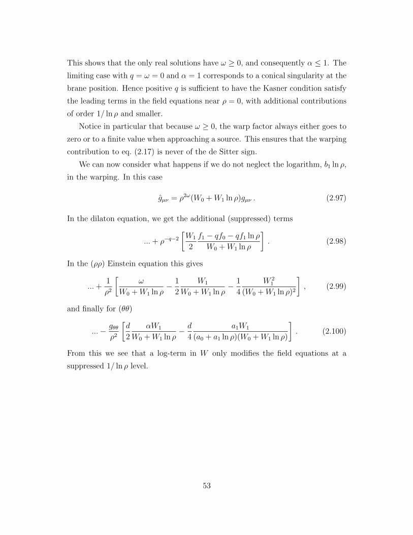
This shows that the only real solutions have ω ≥ 0, and consequently α ≤ 1. The
limiting case with q = ω = 0 and α = 1 corresponds to a conical singularity at the
brane position. Hence positive q is sufficient to have the Kasner condition satisfy
the leading terms in the field equations near ρ = 0, with additional contributions
of order 1/ ln ρ and smaller.
Notice in particular that because ω ≥ 0, the warp factor always either goes to
zero or to a finite value when approaching a source. This ensures that the warping
contribution to eq. (2.17) is never of the de Sitter sign.
We can now consider what happens if we do not neglect the logarithm, b1 ln ρ,
in the warping. In this case
gµν = ρ2ω(W0 +W1 ln ρ)gµν . (2.97)
In the dilaton equation, we get the additional (suppressed) terms
...+ ρ−q−2
[W1
2
f1 − qf0 − qf1 ln ρ
W0 +W1 ln ρ
]. (2.98)
In the (ρρ) Einstein equation this gives
...+1
ρ2
[ω
W0 +W1 ln ρ− 1
2
W1
W0 +W1 ln ρ− 1
4
W 21
(W0 +W1 ln ρ)2
], (2.99)
and finally for (θθ)
...− gθθρ2
[d
2
αW1
W0 +W1 ln ρ− d
4
a1W1
(a0 + a1 ln ρ)(W0 +W1 ln ρ)
]. (2.100)
From this we see that a log-term in W only modifies the field equations at a
suppressed 1/ ln ρ level.
53
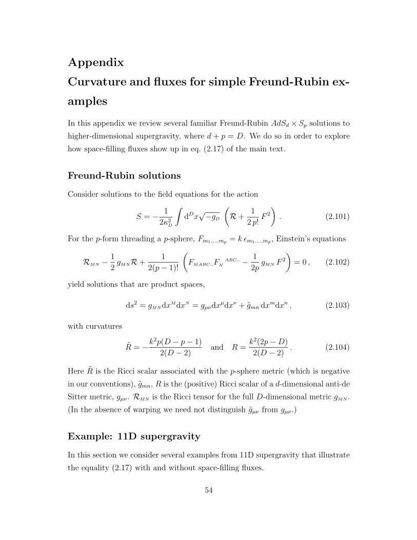
Appendix
Curvature and fluxes for simple Freund-Rubin ex-
amples
In this appendix we review several familiar Freund-Rubin AdSd × Sp solutions to
higher-dimensional supergravity, where d + p = D. We do so in order to explore
how space-filling fluxes show up in eq. (2.17) of the main text.
Freund-Rubin solutions
Consider solutions to the field equations for the action
S = − 1
2κ2D
∫dDx√−gD
(R+
1
2 p!F 2
). (2.101)
For the p-form threading a p-sphere, Fm1.....mp = k εm1.....mp , Einstein’s equations
RMN −1
2gMNR+
1
2(p− 1)!
(FMABC..F
ABC..N − 1
2pgMN F
2
)= 0 , (2.102)
yield solutions that are product spaces,
ds2 = gMNdxMdxN = gµνdxµdxν + gmn dxmdxn , (2.103)
with curvatures
R = −k2p(D − p− 1)
2(D − 2)and R =
k2(2p−D)
2(D − 2). (2.104)
Here R is the Ricci scalar associated with the p-sphere metric (which is negative
in our conventions), gmn, R is the (positive) Ricci scalar of a d-dimensional anti-de
Sitter metric, gµν . RMN is the Ricci tensor for the full D-dimensional metric gMN .
(In the absence of warping we need not distinguish gµν from gµν .)
Example: 11D supergravity
In this section we consider several examples from 11D supergravity that illustrate
the equality (2.17) with and without space-filling fluxes.
54
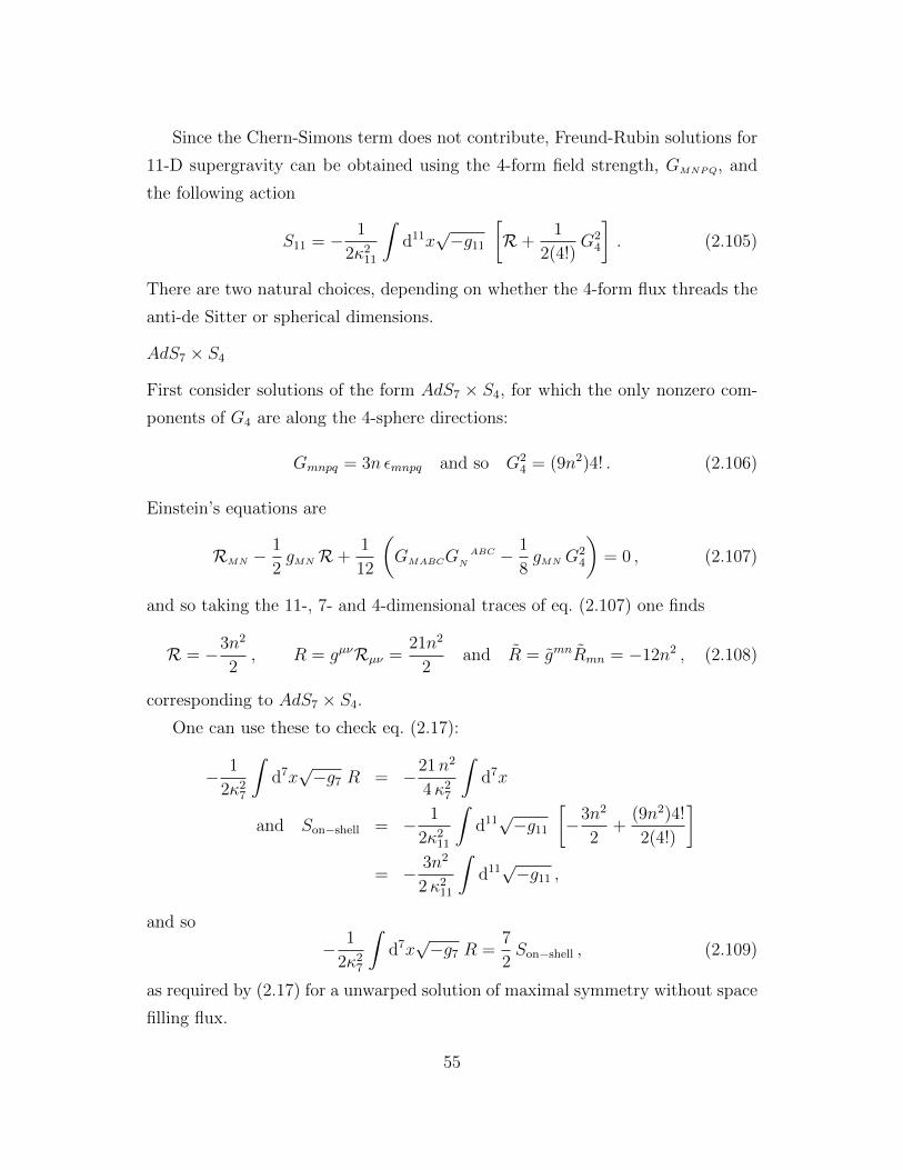
Since the Chern-Simons term does not contribute, Freund-Rubin solutions for
11-D supergravity can be obtained using the 4-form field strength, GMNPQ, and
the following action
S11 = − 1
2κ211
∫d11x√−g11
[R+
1
2(4!)G2
4
]. (2.105)
There are two natural choices, depending on whether the 4-form flux threads the
anti-de Sitter or spherical dimensions.
AdS7 × S4
First consider solutions of the form AdS7 × S4, for which the only nonzero com-
ponents of G4 are along the 4-sphere directions:
Gmnpq = 3n εmnpq and so G24 = (9n2)4! . (2.106)
Einstein’s equations are
RMN −1
2gMN R+
1
12
(GMABCG
ABC
N − 1
8gMN G
24
)= 0 , (2.107)
and so taking the 11-, 7- and 4-dimensional traces of eq. (2.107) one finds
R = −3n2
2, R = gµνRµν =
21n2
2and R = gmnRmn = −12n2 , (2.108)
corresponding to AdS7 × S4.
One can use these to check eq. (2.17):
− 1
2κ27
∫d7x√−g7 R = −21n2
4κ27
∫d7x
and Son−shell = − 1
2κ211
∫d11√−g11
[−3n2
2+
(9n2)4!
2(4!)
]= − 3n2
2κ211
∫d11√−g11 ,
and so
− 1
2κ27
∫d7x√−g7 R =
7
2Son−shell , (2.109)
as required by (2.17) for a unwarped solution of maximal symmetry without space
filling flux.
55

AdS4 × S7
Now consider the solution AdS4×S7, which involves a space-filling flux: Gµνρσ =
3mεµνρσ. From Einstein’s equations one finds
R =3m2
2, R = gmnRmn = −21m2
2and R = gµνRµν = 12m2 . (2.110)
In this case one finds a mismatch between
− 1
2κ24
∫d4x√−g4 R and
4
2Son−shell . (2.111)
This difference is accounted for by including the flux contribution to gµν∂L11/∂gµν ,
which gives a term of the form of eq. (2.22), as required by eq. (2.17).
Alternatively, one can work with a dual Lagrangian containing a kinetic term
for the 7-form, H, that is dual to G:
Sdualized = − 1
2κ211
∫d11x√−g11
[R+
1
2(7!)H2
7
]. (2.112)
In this description the seven form threads only internal directions and has no
space-filling components, and the dualized action evaluates to
− 1
2κ24
∫d4x√−g4R =
4
2S on-shell (dualized) . (2.113)
Recall for these purposes that although dualization is a symmetry of the equations
of motion, it is not a symmetry of the action.
56

Chapter 3
Superspace formulation of SCFTs
with higher spin operators
We now turn to 3d SCFTs. This is a vast arena of current research. These theories
exist aplenty as fixed lines of renormalisation group flows in three dimensions in
the form of superconformal Chern-Simons theories. A classic example, much
studied recently, is ABJ theory [28]. This is an N = 6 superconformal Chern-
Simons theory with the gauge group Uk(N)×U−k(M). We’ll not explicitly study
superconformal Chern-Simons theories in this thesis but our general results on
3d SCFTs apply to these theories in particular. The techniques and formalism
developed in this chapter and the next could probably be used with advantage
in studying higher spin operators/currents and their correlation functions in ABJ
theory and its bulk holographic dual.
In section 3.1 we consider 3d superspace, and the differential form of various
operators which act in it. The construction of superconformally covariant struc-
tures in superspace is reviewed. In section 3.2 on-shell supercurrent multiplets for
higher spin currents in the free theory are constructed out of the superfields. In
section 3.3 we make a few remarks about the structure of anomalous conservation
equations for 3d CFTs and SCFTs with weakly broken higher spin symmetry. In
an appendix we list our conventions and some useful identities.
57

3.1 Superspace
We begin by reviewing superspace in three dimensions and the covariant structures
that it admits, following the paper of Park [36]. Our conventions are summarized
in an appendix to this chapter.
In order to study N = m superconformal field theories in 3 dimensions we em-
ploy a superspace whose coordinates are the 3 spacetime coordinates xµ together
with the 2m fermionic coordinates θaα. Here α = 1, 2 is a spacetime spinor index
while a = 1 . . .m is the R-symmetry index, where the θs (and the supercharges
Qaαs) are Majorana spinors that lie in the vector representation of the R-symmetry
group SO(N ). The superconformal algebra, listed in (3.56) in the appendix, is
implemented in superspace by the construction
Pµ = −i∂µ,
Mµν = −i(xµ∂ν − xν∂µ −
1
2εµνρ(γ
ρ) βα θ
aβ
∂
∂θaα
)+Mµν ,
D = −i(xν∂ν +
1
2θαa
∂
∂θαa
)+ ∆,
Kµ = −i((
x2 +(θaθa)2
16
)∂µ − 2xµ
(x · ∂ + θαa
∂
∂θαa
)+ (θaX+γµ)β
∂
∂θβa
)= xνMνµ − xµD +
i
2(θaγµX)α
∂
∂θαa− i
16(θaθa)2∂µ +
(θaθa)
4(θbγµ)α
∂
∂θαb,
Qaα =
∂
∂θαa− i
2θβa(γµ)βα∂µ,
Saα = −(X+) βα Q
aβ − iθaθb
∂
∂θαb− iθaαθbβ
∂
∂θβb+i
2(θbθb)
∂
∂θαa
= −(X−) βα
∂
∂θβa+θaα2D +
1
4εµνρ(γ
ρθa)αMµν − (θbθb)
8θaβ∂βα −
3i
4
(θaαθ
∂
∂θ+ θaθb
∂
∂θαb
),
Iab = −i(θa
∂
∂θb− θb ∂
∂θa
)+ Iab .
(3.1)
Here the derivative expressions act on superspace coordinates while the operators
M, ∆ and Iab act on the operators (states) which carry tensor structure, non-zero
scaling dimensions and transform non-trivially under R-symmetry. All indices
are contracted in matrix notation (the spinors are contracted from north-west to
58
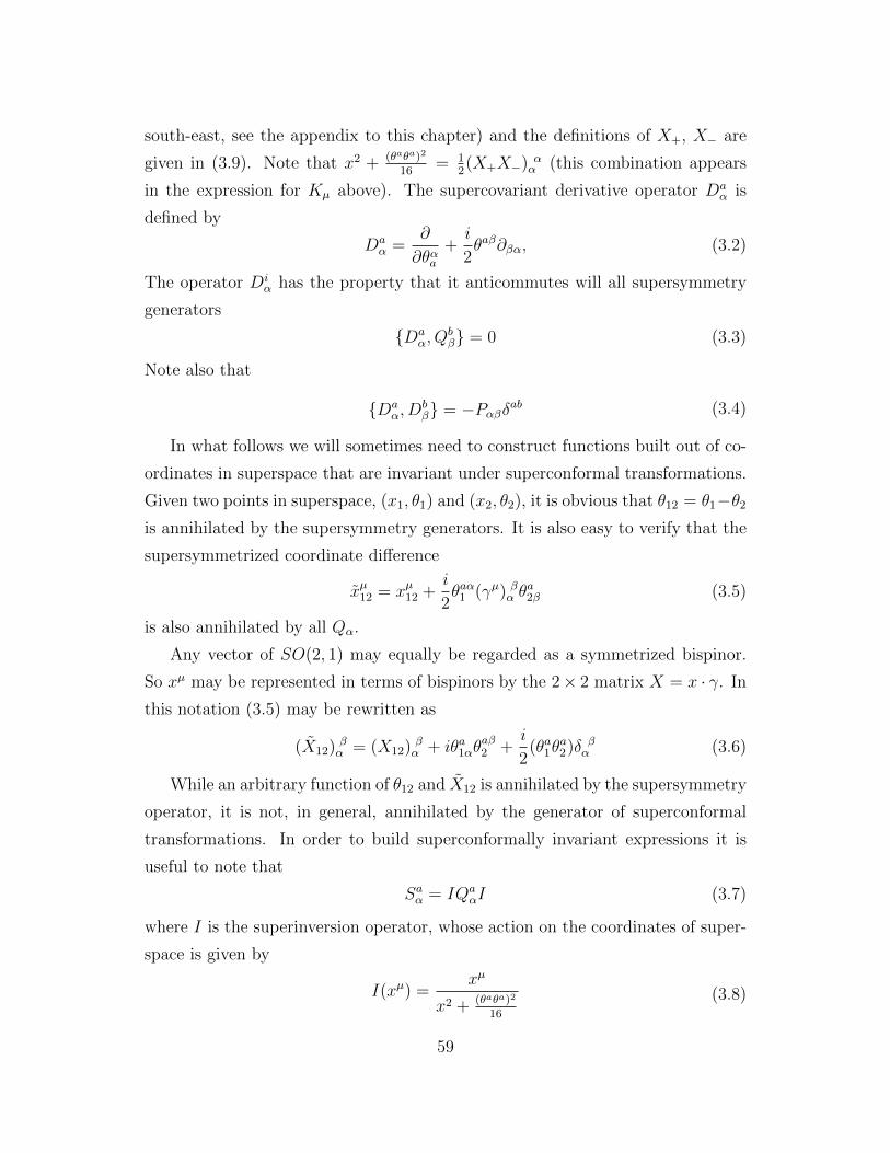
south-east, see the appendix to this chapter) and the definitions of X+, X− are
given in (3.9). Note that x2 + (θaθa)2
16= 1
2(X+X−) α
α (this combination appears
in the expression for Kµ above). The supercovariant derivative operator Daα is
defined by
Daα =
∂
∂θαa+i
2θaβ∂βα, (3.2)
The operator Diα has the property that it anticommutes will all supersymmetry
generators
Daα, Q
bβ = 0 (3.3)
Note also that
Daα, D
bβ = −Pαβδab (3.4)
In what follows we will sometimes need to construct functions built out of co-
ordinates in superspace that are invariant under superconformal transformations.
Given two points in superspace, (x1, θ1) and (x2, θ2), it is obvious that θ12 = θ1−θ2
is annihilated by the supersymmetry generators. It is also easy to verify that the
supersymmetrized coordinate difference
xµ12 = xµ12 +i
2θaα1 (γµ) βα θ
a2β (3.5)
is also annihilated by all Qα.
Any vector of SO(2, 1) may equally be regarded as a symmetrized bispinor.
So xµ may be represented in terms of bispinors by the 2× 2 matrix X = x · γ. In
this notation (3.5) may be rewritten as
(X12) βα = (X12) βα + iθa1αθaβ2 +
i
2(θa1θ
a2)δ β
α (3.6)
While an arbitrary function of θ12 and X12 is annihilated by the supersymmetry
operator, it is not, in general, annihilated by the generator of superconformal
transformations. In order to build superconformally invariant expressions it is
useful to note that
Saα = IQaαI (3.7)
where I is the superinversion operator, whose action on the coordinates of super-
space is given by
I(xµ) =xµ
x2 + (θaθa)2
16
(3.8)
59
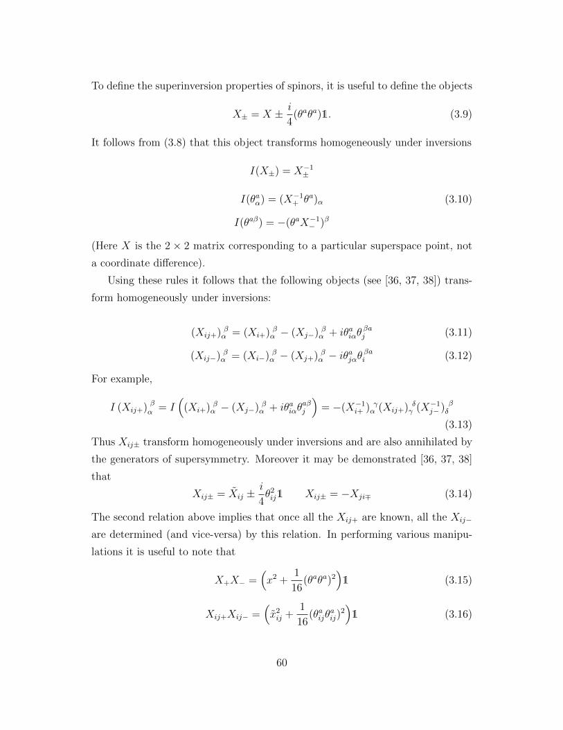
To define the superinversion properties of spinors, it is useful to define the objects
X± = X ± i
4(θaθa)1. (3.9)
It follows from (3.8) that this object transforms homogeneously under inversions
I(X±) = X−1±
I(θaα) = (X−1+ θa)α (3.10)
I(θaβ) = −(θaX−1− )β
(Here X is the 2 × 2 matrix corresponding to a particular superspace point, not
a coordinate difference).
Using these rules it follows that the following objects (see [36, 37, 38]) trans-
form homogeneously under inversions:
(Xij+) βα = (Xi+) βα − (Xj−) βα + iθaiαθβaj (3.11)
(Xij−) βα = (Xi−) βα − (Xj+) βα − iθajαθβai (3.12)
For example,
I (Xij+) βα = I(
(Xi+) βα − (Xj−) βα + iθaiαθaβj
)= −(X−1
i+ ) γα (Xij+) δ
γ (X−1j− ) β
δ
(3.13)
Thus Xij± transform homogeneously under inversions and are also annihilated by
the generators of supersymmetry. Moreover it may be demonstrated [36, 37, 38]
that
Xij± = Xij ±i
4θ2ij1 Xij± = −Xji∓ (3.14)
The second relation above implies that once all the Xij+ are known, all the Xij−
are determined (and vice-versa) by this relation. In performing various manipu-
lations it is useful to note that
X+X− =(x2 +
1
16(θaθa)2
)1 (3.15)
Xij+Xij− =(x2ij +
1
16(θaijθ
aij)
2)1 (3.16)
60

so that
(X±)−1 =X∓
x2 + 116
(θaθa)2
(Xij±)−1 =Xij∓
x2ij + 1
16(θaijθ
aij)
2
(3.17)
(note that the the R-symmetry index a is summed over but that, throughout,
i, j (= 1, 2, 3) label points in superspace and are not summed over).
There also exist fermionic covariant structures (which are identically zero in
the non-supersymmetric case) which are constructed out of the superspace co-
ordinates as follows [36, 37, 38]:
Θa1α =
((X−1
21+θa21)α − (X−1
31+θa31)α
)(3.18)
Θ2, Θ3 are defined similarly. Its transformation properties under superinversion
are
Θaiα → −(Xi−) βα Θb
iβIab Θαa
i → ITab Θβ bi (Xi+) αβ (3.19)
The basic covariant structures Xij±, Θaiα are annihilated by the generators
of supersymmetry. For this reason they form the basic building blocks for the
construction of superconformal invariants, as we will explain in a later section.
Polarization spinors: Since we will be dealing extensively with higher spin
operators and their correlators, it will be useful to adopt a formalism, developed in
[35], in which the information about the tensor structure is encoded in polarization
spinors: λα. These auxiliary objects are book-keeping devices to keep track of the
tensorial nature of correlators in an efficient manner. They are defined to be real,
bosonic, two-component objects transforming as spinors of the 3d Lorentz group
(see [35]). Being spinors in 2+1 dimensions fixes their transformation law under
superinversions:
λα → (X−1+ λ)α , λβ → −(λX−1
− )β (3.20)
(This is the same as the transformation law of the θ’s).
A higher spin primary operator Jµ1µ2.....µs with spin s can be represented
in spinor components by Jα1α2.....α2s ≡ (σµ1)α1α2(σµ2)α3α4 ....(σ
µs)α2s−1α2sJµ1µ2.....µs .
We note that this represents an operator supermultiplet in contradistinction to [35]
61
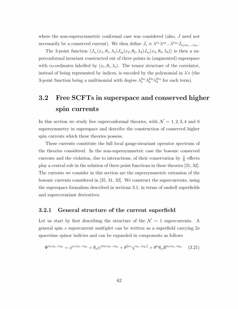
where the non-supersymmetric conformal case was considered (also, J need not
necessarily be a conserved current). We then define Js ≡ λα1λα2 ...λα2sJα1α2.....α2s .
The 3-point function 〈Js1(x1, θ1, λ1)Js2(x2, θ2, λ2)Js3(x3, θ3, λ3)〉 is then a su-
perconformal invariant constructed out of three points in (augmented) superspace
with co-ordinates labelled by (xi, θi, λi). The tensor structure of the correlator,
instead of being represented by indices, is encoded by the polynomial in λ’s (the
3-point function being a multinomial with degree λ2s11 λ2s2
2 λ2s33 for each term).
3.2 Free SCFTs in superspace and conserved higher
spin currents
In this section we study free superconformal theories, with N = 1, 2, 3, 4 and 6
supersymmetry in superspace and describe the construction of conserved higher
spin currents which these theories possess.
These currents constitute the full local gauge-invariant operator spectrum of
the theories considered. In the non-supersymmetric case the bosonic conserved
currents and the violation, due to interactions, of their conservation by 1N
effects
play a central role in the solution of three point functions in these theories [31, 32].
The currents we consider in this section are the supersymmetric extension of the
bosonic currents considered in [35, 31, 32]. We construct the supercurrents, using
the superspace formalism described in sections 3.1, in terms of onshell superfields
and supercovariant derivatives.
3.2.1 General structure of the current superfield
Let us start by first describing the structure of the N = 1 supercurrents. A
general spin s supercurrent multiplet can be written as a superfield carrying 2s
spacetime spinor indicies and can be expanded in components as follows
Φα1α2...α2s = φα1α2...α2s + θαψαα1α2...α2s + θα1χα2...α2s + θαθαB
α1α2...α2s (3.21)
62
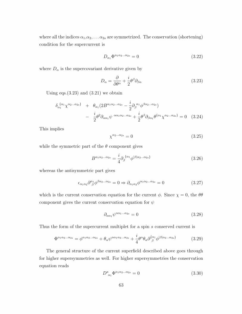
where all the indices α1,α2, . . . α2s are symmetrized. The conservation (shortening)
condition for the supercurrent is
Dα1Φα1α2...α2s = 0 (3.22)
where Dα is the supercovariant derivative given by
Dα =∂
∂θα+i
2θβ∂βα (3.23)
Using eqs.(3.23) and (3.21) we obtain
δ α1α1
χα2...α2s + θα1(2Bα1α2...α2s − i
2∂ α1β φβα2...α2s)
− i
2θ2∂αα1ψ
αα1α2...α2s +i
2θβ∂βα1θ
α1χα2...α2s = 0 (3.24)
This implies
χα2...α2s = 0 (3.25)
while the symmetric part of the θ component gives
Bα1α2...α2s =i
4∂α1
β φ|β|α2...α2s (3.26)
whereas the antisymmetric part gives
εα1α2∂α1β φ
βα2...α2s = 0⇒ ∂α1α2φα1α2...α2s = 0 (3.27)
which is the current conservation equation for the current φ. Since χ = 0, the θθ
component gives the current conservation equation for ψ
∂αα1ψαα1...α2s = 0 (3.28)
Thus the form of the supercurrent multiplet for a spin s conserved current is
Φα1α2...α2s = φα1α2...α2s + θαψαα1α2...α2s +
i
4θαθα∂
α1
β φ|β|α2...α2s (3.29)
The general structure of the current superfield described above goes through
for higher supersymmetries as well. For higher supersymmetries the conservation
equation reads
Daα1
Φα1α2...α2s = 0 (3.30)
63

where a = 1, 2 . . .N is the R-symmetry index1. In the case of an N = m spin-
s current multiplet, the currents φα1α2...α2s and ψαα1α2...α2s are themselves N =
m − 1 spin s and spin s + 12
conserved current superfields (depending on the
grassmann coordinates θaα: a = 1, . . .m− 1) while the θα in (3.29) is the left over
grassmann coordinate θmα . Thus we see the general structure of the supercurrent
multiplets: AnN = m spin s supercurrent multiplet breaks up into twoN = m−1
supercurrents with spins s and s+ 12
respectively.
This structure can be used to express higher supercurrents superfields in term
of components. For instance, theN = 2 spin s currents superfield can be expanded
in components as follows
Φα1α2...α2s = ϕα1α2...α2s + θaα(ψa)αα1α2...α2s +1
2εabθ
aαθ
bβAαβα1α2...α2s
+ term involving derivatives of ϕ, ψa and A(3.31)
where a, b are R-symmetry indicies and take values in 1, 2. The conformal
state content so obtained, namely (ϕ, ψ1, ψ2,A) above, match exactly with the
decomposition of spin s supercurrent multiplet into conformal multiplets.
3.2.2 Free field construction of currents
In this section we give an explicit construction of the conserved higher spin su-
percurrents in term of superfields for N = 1, 2, 3, 4, 6 free SCFTs. 2
N = 1
In a free field theory the exactly conserved higher spin currents are bilinear in the
free fields with symmetrised derivatives. For example, in the free bosonic O(N)
vector models the currents have the schematic form: J(s) ∼ φi∂sφi + ... where
any number of the s derivatives can act left or right and the whole expression
is symmetrised and traceless. The coefficients in this linear combination can be
1Note that for N > 1, (3.30) is true only for R-symmetry singlet currents. For currents
carrying non-trivial R-symmetry representation the shortening condition is different. In this
paper we will only need the shortening condition (3.30).2This part was worked out by V. Umesh and T. Sharma in collaboration with Shiraz Min-
walla. It is included here for the sake of completeness.
64
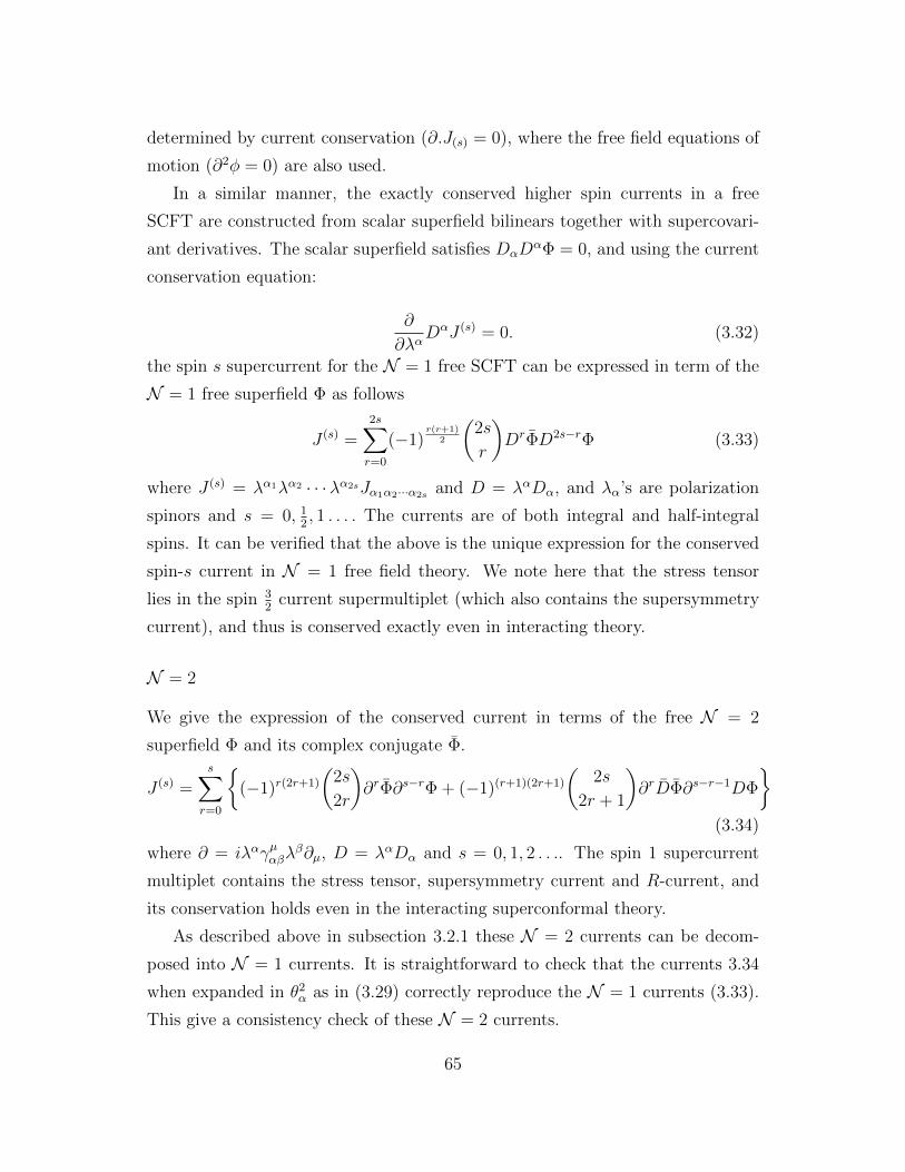
determined by current conservation (∂.J(s) = 0), where the free field equations of
motion (∂2φ = 0) are also used.
In a similar manner, the exactly conserved higher spin currents in a free
SCFT are constructed from scalar superfield bilinears together with supercovari-
ant derivatives. The scalar superfield satisfies DαDαΦ = 0, and using the current
conservation equation:
∂
∂λαDαJ (s) = 0. (3.32)
the spin s supercurrent for the N = 1 free SCFT can be expressed in term of the
N = 1 free superfield Φ as follows
J (s) =2s∑r=0
(−1)r(r+1)
2
(2s
r
)DrΦD2s−rΦ (3.33)
where J (s) = λα1λα2 · · ·λα2sJα1α2···α2s and D = λαDα, and λα’s are polarization
spinors and s = 0, 12, 1 . . . . The currents are of both integral and half-integral
spins. It can be verified that the above is the unique expression for the conserved
spin-s current in N = 1 free field theory. We note here that the stress tensor
lies in the spin 32
current supermultiplet (which also contains the supersymmetry
current), and thus is conserved exactly even in interacting theory.
N = 2
We give the expression of the conserved current in terms of the free N = 2
superfield Φ and its complex conjugate Φ.
J (s) =s∑r=0
(−1)r(2r+1)
(2s
2r
)∂rΦ∂s−rΦ + (−1)(r+1)(2r+1)
(2s
2r + 1
)∂rDΦ∂s−r−1DΦ
(3.34)
where ∂ = iλαγµαβλβ∂µ, D = λαDα and s = 0, 1, 2 . . .. The spin 1 supercurrent
multiplet contains the stress tensor, supersymmetry current and R-current, and
its conservation holds even in the interacting superconformal theory.
As described above in subsection 3.2.1 these N = 2 currents can be decom-
posed into N = 1 currents. It is straightforward to check that the currents 3.34
when expanded in θ2α as in (3.29) correctly reproduce the N = 1 currents (3.33).
This give a consistency check of these N = 2 currents.
65
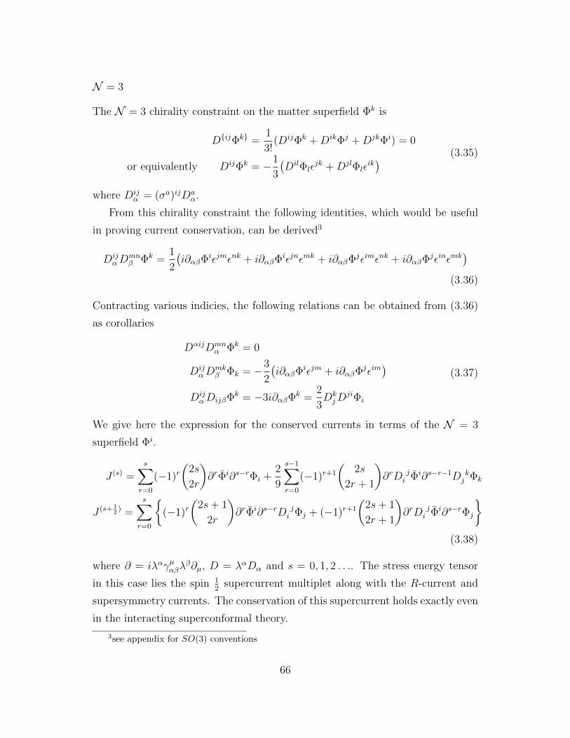
N = 3
The N = 3 chirality constraint on the matter superfield Φk is
DijΦk =1
3!(DijΦk +DikΦj +DjkΦi) = 0
or equivalently DijΦk = −1
3
(DilΦlε
jk +DjlΦlεik) (3.35)
where Dijα = (σa)ijDa
α.
From this chirality constraint the following identities, which would be useful
in proving current conservation, can be derived3
DijαD
mnβ Φk =
1
2
(i∂αβΦiεjmεnk + i∂αβΦiεjnεmk + i∂αβΦjεimεnk + i∂αβΦjεinεmk
)(3.36)
Contracting various indicies, the following relations can be obtained from (3.36)
as corollaries
DαijDmnα Φk = 0
DijαD
mkβ Φk = −3
2
(i∂αβΦiεjm + i∂αβΦjεim
)DijαDijβΦk = −3i∂αβΦk =
2
3DkjD
jiΦi
(3.37)
We give here the expression for the conserved currents in terms of the N = 3
superfield Φi.
J (s) =s∑r=0
(−1)r(
2s
2r
)∂rΦi∂s−rΦi +
2
9
s−1∑r=0
(−1)r+1
(2s
2r + 1
)∂rD j
i Φi∂s−r−1D kj Φk
J (s+ 12
) =s∑r=0
(−1)r
(2s+ 1
2r
)∂rΦi∂s−rD j
i Φj + (−1)r+1
(2s+ 1
2r + 1
)∂rD j
i Φi∂s−rΦj
(3.38)
where ∂ = iλαγµαβλβ∂µ, D = λαDα and s = 0, 1, 2 . . .. The stress energy tensor
in this case lies the spin 12
supercurrent multiplet along with the R-current and
supersymmetry currents. The conservation of this supercurrent holds exactly even
in the interacting superconformal theory.
3see appendix for SO(3) conventions
66
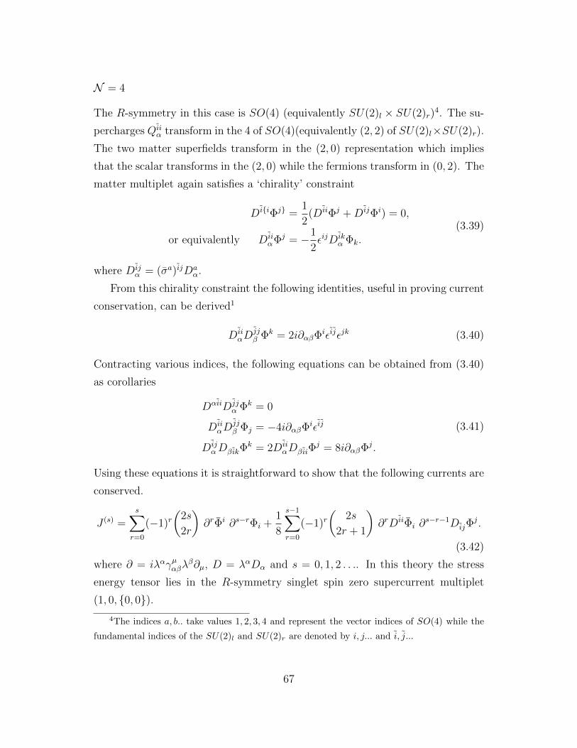
N = 4
The R-symmetry in this case is SO(4) (equivalently SU(2)l × SU(2)r)4. The su-
percharges Qiiα transform in the 4 of SO(4)(equivalently (2, 2) of SU(2)l×SU(2)r).
The two matter superfields transform in the (2, 0) representation which implies
that the scalar transforms in the (2, 0) while the fermions transform in (0, 2). The
matter multiplet again satisfies a ‘chirality’ constraint
DiiΦj =1
2(DiiΦj +DijΦi) = 0,
or equivalently DiiαΦj = −1
2εijDik
α Φk.(3.39)
where Dijα = (σa)ijDa
α.
From this chirality constraint the following identities, useful in proving current
conservation, can be derived1
DiiαD
jjβ Φk = 2i∂αβΦiεijεjk (3.40)
Contracting various indices, the following equations can be obtained from (3.40)
as corollaries
DαiiDjjα Φk = 0
DiiαD
jjβ Φj = −4i∂αβΦiεij
DijαDβikΦ
k = 2DiiαDβiiΦ
j = 8i∂αβΦj.
(3.41)
Using these equations it is straightforward to show that the following currents are
conserved.
J (s) =s∑r=0
(−1)r(
2s
2r
)∂rΦi ∂s−rΦi +
1
8
s−1∑r=0
(−1)r(
2s
2r + 1
)∂rDiiΦi ∂
s−r−1DijΦj.
(3.42)
where ∂ = iλαγµαβλβ∂µ, D = λαDα and s = 0, 1, 2 . . .. In this theory the stress
energy tensor lies in the R-symmetry singlet spin zero supercurrent multiplet
(1, 0, 0, 0).4The indices a, b.. take values 1, 2, 3, 4 and represent the vector indices of SO(4) while the
fundamental indices of the SU(2)l and SU(2)r are denoted by i, j... and i, j...
67

N = 6
The field content of this theory is double of the field content of the N = 4 theory.
In N = 2 language the field content is 2 chiral and 2 antichiral multiplets in
fundamental of the gauge group. The R-symmetry in this theory is SO(6) (≡SU(4)) under which the supercharges transform in vector representation (6 of
SO(6)) while the 2+2 chiral and antichiral multiplets transform in chiral spinor
representation (4 of SU(4)).
The N = 6 shortening (chirality) condition on the matter multiplet is5
DijαΦk = Djk
α Φi = Dkiα Φj
or equivalently DaαΦk = − 1
10DbαΦl(γab) k
l
(3.43)
From this chirality constraint the following identities, which are useful in prov-
ing current conservation, can be derived2
DaαD
bβΦk =
i
2∂αβΦkδab +
i
4∂αβΦl(γab) k
l ,
or equivalently DijαD
mnβ Φk = −i∂αβ
(εijmnΦk + εkjmnΦi + εikmnΦj − εijknΦm − εijmkΦn
)(3.44)
Taking the complex conjugate of equations (3.43) and (3.44), and using the
property that γab and γab are antihermitian, we get
Dijα Φk =
1
3
(DilαΦlδ
jk −D
jlα Φlδ
ik
)or equivalently Da
αΦk =1
10Dbα(γab) l
k Φl
(3.45)
and
DaαD
bβΦk =
i
2∂αβΦkδ
ab − i
4∂αβ(γab) l
k Φl,
or equivalently DijαD
mnβ Φk = −i∂αβ
(εijmnΦk − εljmnΦlδ
ik − εilmnΦlδ
jk + εijlnΦlδ
mk + εijmlΦlδ
nk
)(3.46)
5Here we revert back to lower case letters for the SU(4) indices i, j (taking values 1, . . . 4)
as there is no confusion with other R indices.
68
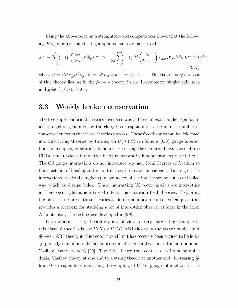
Using the above relation a straightforward computation shows that the follow-
ing R-symmetry singlet integer spin currents are conserved
J (s) =s∑r=0
(−1)r(
2s
2r
)∂rΦp ∂
s−rΦp− 1
24
s−1∑r=0
(−1)r+1
(2s
2r + 1
)εijkl ∂
rDijΦp ∂s−r−1DklΦp.
(3.47)
where ∂ = iλαγµαβλβ∂µ, D = λαDα and s = 0, 1, 2 . . .. The stress-energy tensor
of this theory lies, as in the N = 4 theory, in the R-symmetry singlet spin zero
multiplet (1, 0, 0, 0, 0).
3.3 Weakly broken conservation
The free superconformal theories discussed above have an exact higher spin sym-
metry algebra generated by the charges corresponding to the infinite number of
conserved currents that these theories possess. These free theories can be deformed
into interacting theories by turning on U(N) Chern-Simons (CS) gauge interac-
tions, in a supersymmetric fashion and preserving the conformal invariance of free
CFTs, under which the matter fields transform in fundamental representations.
The CS gauge interactions do not introduce any new local degrees of freedom so
the spectrum of local operators in the theory remains unchanged. Turning on the
interactions breaks the higher spin symmetry of the free theory but in a controlled
way which we discuss below. These interacting CS vector models are interesting
in there own right as non trivial interacting quantum field theories. Exploring
the phase structure of these theories at finite temperature and chemical potential,
provides a platform for studying a lot of interesting physics, at least in the large
N limit, using the techniques developed in [29].
From a more string theoretic point of view, a very interesting example of
this class of theories is the U(N) × U(M) ABJ theory in the vector model limitMN→ 0. ABJ theory in this vector model limit has recently been argued to be holo-
graphically dual a non-abelian supersymmetric generalization of the non-minimal
Vasiliev theory in AdS4 [29]. The ABJ theory thus connects, as its holographic
duals, Vasiliev theory at one end to a string theory at another end. Increasing MN
from 0 corresponds to increasing the coupling of U(M) gauge interactions in the
69
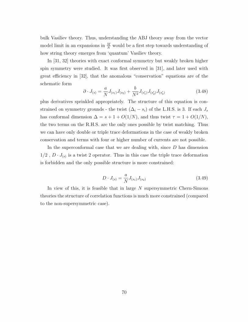
bulk Vasiliev theory. Thus, understanding the ABJ theory away from the vector
model limit in an expansions in MN
would be a first step towards understanding of
how string theory emerges from ‘quantum’ Vasiliev theory.
In [31, 32] theories with exact conformal symmetry but weakly broken higher
spin symmetry were studied. It was first observed in [31], and later used with
great efficiency in [32], that the anomalous “conservation” equations are of the
schematic form
∂ · J(s) =a
NJ(s1)J(s2) +
b
N2J(s′1)J(s′2)J(s′3) (3.48)
plus derivatives sprinkled appropriately. The structure of this equation is con-
strained on symmetry grounds - the twist (∆i − si) of the L.H.S. is 3. If each Js
has conformal dimension ∆ = s + 1 + O(1/N), and thus twist τ = 1 + O(1/N),
the two terms on the R.H.S. are the only ones possible by twist matching. Thus
we can have only double or triple trace deformations in the case of weakly broken
conservation and terms with four or higher number of currents are not possible.
In the superconformal case that we are dealing with, since D has dimension
1/2 , D · J(s) is a twist 2 operator. Thus in this case the triple trace deformation
is forbidden and the only possible structure is more constrained:
D · J(s) =a
NJ(s1)J(s2) (3.49)
In view of this, it is feasible that in large N supersymmetric Chern-Simons
theories the structure of correlation functions is much more constrained (compared
to the non-supersymmetric case).
70
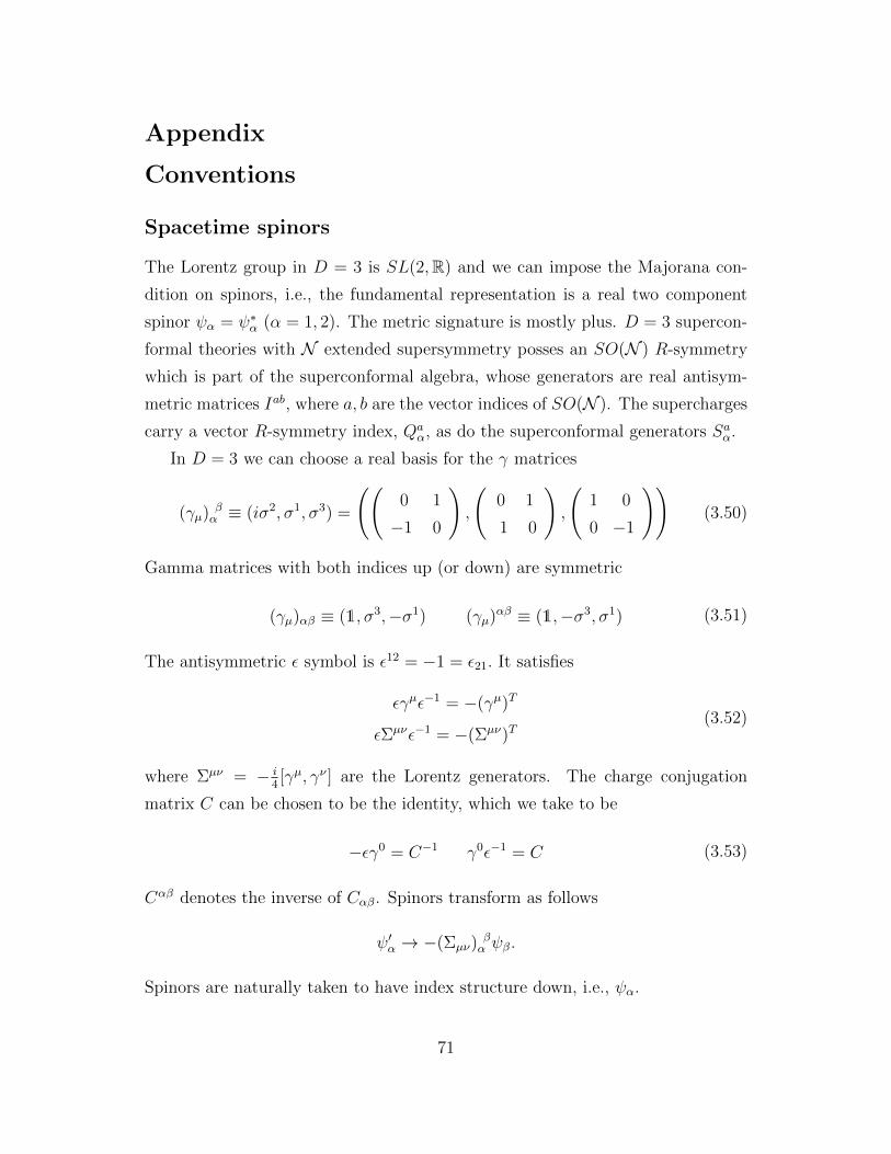
Appendix
Conventions
Spacetime spinors
The Lorentz group in D = 3 is SL(2,R) and we can impose the Majorana con-
dition on spinors, i.e., the fundamental representation is a real two component
spinor ψα = ψ∗α (α = 1, 2). The metric signature is mostly plus. D = 3 supercon-
formal theories with N extended supersymmetry posses an SO(N ) R-symmetry
which is part of the superconformal algebra, whose generators are real antisym-
metric matrices Iab, where a, b are the vector indices of SO(N ). The supercharges
carry a vector R-symmetry index, Qaα, as do the superconformal generators Saα.
In D = 3 we can choose a real basis for the γ matrices
(γµ) βα ≡ (iσ2, σ1, σ3) =
((0 1
−1 0
),
(0 1
1 0
),
(1 0
0 −1
))(3.50)
Gamma matrices with both indices up (or down) are symmetric
(γµ)αβ ≡ (1, σ3,−σ1) (γµ)αβ ≡ (1,−σ3, σ1) (3.51)
The antisymmetric ε symbol is ε12 = −1 = ε21. It satisfies
εγµε−1 = −(γµ)T
εΣµνε−1 = −(Σµν)T(3.52)
where Σµν = − i4[γµ, γν ] are the Lorentz generators. The charge conjugation
matrix C can be chosen to be the identity, which we take to be
−εγ0 = C−1 γ0ε−1 = C (3.53)
Cαβ denotes the inverse of Cαβ. Spinors transform as follows
ψ′α → −(Σµν)βα ψβ.
Spinors are naturally taken to have index structure down, i.e., ψα.
71

The raising and lowering conventions are
ψβ = εβαψα
ψα = εαβψβ
(3.54)
There is now only one way to suppress contracted spinor indices,
ψχ = ψαχα,
and this leads to a sign when performing Hermitian conjugation
(ψχ)∗ = −χ∗ψ∗.
The γ matrices satisfy
(γµγν)βα = ηµνδ
βα + εµνρ(γ
ρ) βα (3.55)
where εµνρ is the Levi-Civita symbol, and we set ε012 = 1 (ε012 = −1). The
superconformal algebra is given below:
[Mµν ,Mρλ] = i (ηµρMνλ − ηνρMµλ − ηµλMνρ + ηνλMµρ) ,
[Mµν , Pλ] = i(ηµλPν − ηνλPµ),
[Mµν , Kλ] = i(ηµλKν − ηνλKµ),
[D,Pµ] = iPµ , [D,Kµ] = −iKµ,
[Pµ, Kν ] = 2i(ηµνD −Mµν),
[Iab, Icd] = i (δacIbd − δbcIad − δadIbc + δbdIac) ,
Qaα, Q
bβ = (γµ)αβPµδ
ab,
[Iab, Qαc ] = i(δacQ
αb − δbcQα
a ),
Saα, Sbβ = (γµ)αβKµδab,
[Iab, Sαc ] = i(δacS
αb − δbcSαa ),
[Kµ, Qaα] = i(γµ) β
α Saβ,
[Pµ, Saα] = i(γµ) β
α Qaβ,
[D,Qaα] =
i
2Qaα , [D,Saα] = − i
2Saα,
[Mµν , Qaα] = −(Σµν)
βα Q
aβ,
[Mµν , Saα] = −(Σµν)
βα S
aβ,
Qaα, S
bβ =
(εβαD −
1
2εµνρ(γ
ρ)αβMµν
)δab + εβαI
ab.
(3.56)
72

All other (anti)-commutators vanish.
R-symmetry
SO(3)
Gamma matrices are chosen to be the sigma matrices
(σa) ji =
((0 1
1 0
),
(0 −ii 0
),
(1 0
0 −1
)). (3.57)
Indicies are raised and lowered by ε12 = −1 = −ε12. Note that σ matrices with
both lower or both upper indicies are symmetric.
The following identities are useful
εijφk + εjkφi + εkiφj = 0,
εijεkl = δilδjk − δ
ikδjl ,
εijεkl = εikεjl − εilεjk, (same for upper indices)
(σa) ji (σa) l
k = 2δliδjk − δ
ji δlk
(σa)ij(σa)kl = −(2εilεjk + εijεkl) = −(εikεjl + εilεjk)
(3.58)
SO(4)
Gamma matrices are chosen to be
Γa =
(0 σa
σa 0
)for a= 1,2. . . 4
where (σa) ii = (σ1, σ2, σ3, i12), (σa) i
i= (σ1, σ2, σ3,−i12).
(3.59)
Indicies are raised and lowered by ε12 = −ε12 = −1 = ε12 = −ε12. With these
definitions, the following identities would be useful.
(σa)ii = (σaT )ii((σa)T = −εσaε−1
),
(σa) ii (σa) j
j= 2δ i
jδji ,
(σa)ii(σa)jj = −2εijεij, (σa)ii(σa)jj = −2εijεij.
(3.60)
73
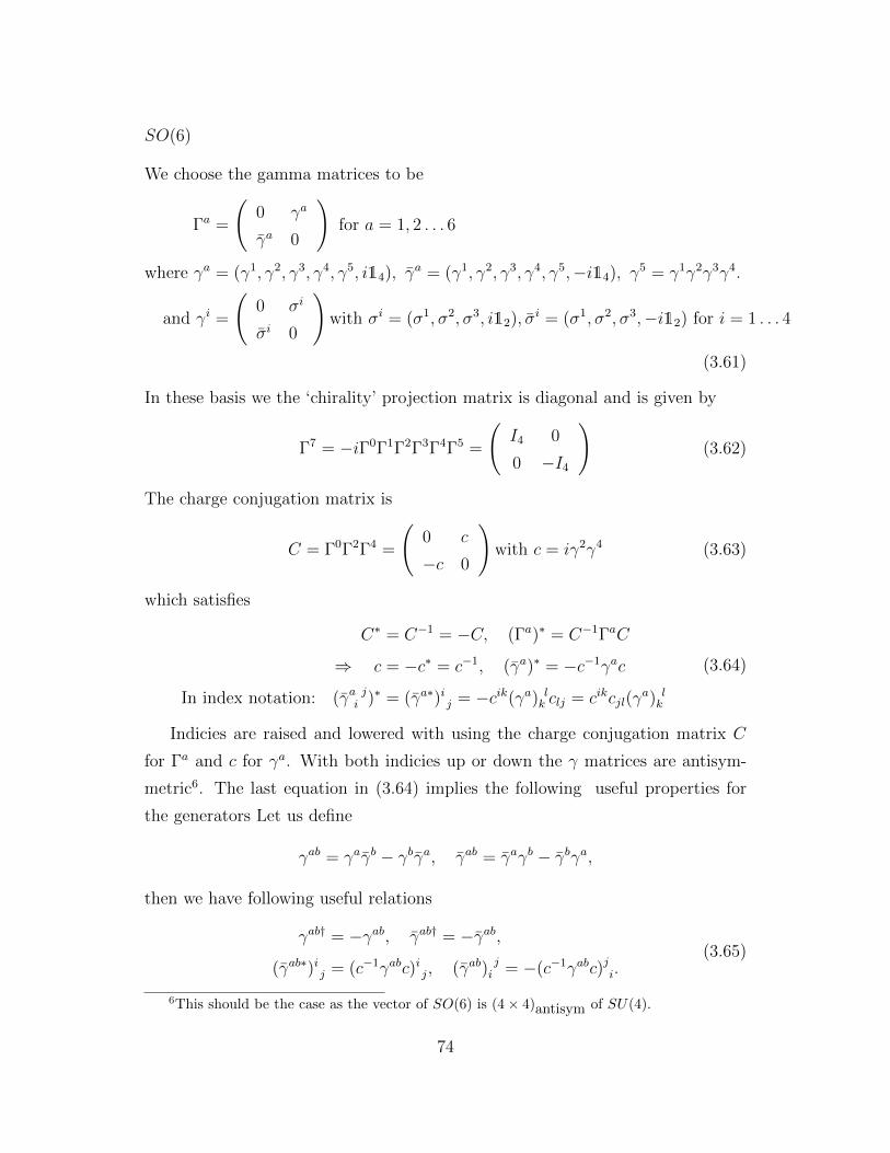
SO(6)
We choose the gamma matrices to be
Γa =
(0 γa
γa 0
)for a = 1, 2 . . . 6
where γa = (γ1, γ2, γ3, γ4, γ5, i14), γa = (γ1, γ2, γ3, γ4, γ5,−i14), γ5 = γ1γ2γ3γ4.
and γi =
(0 σi
σi 0
)with σi = (σ1, σ2, σ3, i12), σi = (σ1, σ2, σ3,−i12) for i = 1 . . . 4
(3.61)
In these basis we the ‘chirality’ projection matrix is diagonal and is given by
Γ7 = −iΓ0Γ1Γ2Γ3Γ4Γ5 =
(I4 0
0 −I4
)(3.62)
The charge conjugation matrix is
C = Γ0Γ2Γ4 =
(0 c
−c 0
)with c = iγ2γ4 (3.63)
which satisfies
C∗ = C−1 = −C, (Γa)∗ = C−1ΓaC
⇒ c = −c∗ = c−1, (γa)∗ = −c−1γac
In index notation: (γa ji )∗ = (γa∗)i j = −cik(γa) l
k clj = cikcjl(γa) lk
(3.64)
Indicies are raised and lowered with using the charge conjugation matrix C
for Γa and c for γa. With both indicies up or down the γ matrices are antisym-
metric6. The last equation in (3.64) implies the following useful properties for
the generators Let us define
γab = γaγb − γbγa, γab = γaγb − γbγa,
then we have following useful relations
γab† = −γab, γab† = −γab,
(γab∗)i j = (c−1γabc)i j, (γab) ji = −(c−1γabc)ji.
(3.65)
6This should be the case as the vector of SO(6) is (4× 4)antisym of SU(4).
74

The first line says that the generators of SO(6) transformation are Hermitian7
while the two equation in the second line follows from (3.64).
The following identities are useful8:
γaij = γaij + 2δa0cij, (γa) ji = (γa) j
i − 2δa0δji ,
γaijγakl = −2εijkl = 2(cikcjl − cilcjk − cijckl),
γaij γakl = −2εijkl + 2cijckl = 2(cikcjl − cilcjk),
(γa)ij(γa)kl = 2δikδjl − 2δilδ
jk,
(γab)ji (γab)lk = −32δliδ
jk + 8δji δ
lk,
(3.66)
Useful relations
Some useful relations and identities are given below
εαβ∂
∂θaβ= − ∂
∂θaα(3.67)
(γµ) βα (γµ) ρ
σ = 2δ ρα δ
βσ − δ β
α δρσ (3.68)
θαθβ =1
2εαβθθ, θαθβ = −1
2εαβθθ (3.69)
θ1αθβ2 + θ2αθ
β1 + (θ1θ2)δβα = 0 (3.70)
X2 ≡ X βα X
αβ = 2xµx
µ ≡ 2x2 , X βα X
γβ = x2δγα =
X2
2δγα (3.71)
D1αX−∆12 = i∆(X12) βα (θ12)β (3.72)
D1α(X12) γβ = −iδγα(θ12)β +i
2δγβ(θ12)α (3.73)
D1α(X12−) γβ = −iδγαθ12β , D1α(X12+) γβ = iεαβθγ12 (3.74)
7The generator of SO(6) acting on chiral and antichiral transformation are respectively
− i4γ
ab and − i4 γ
ab
8Note that representation theory (SU(4)) wise C shouldn’t be used to raise or lower indicies
as it is not an invariant tensor of SU(4). Only εijkl and εijkl(which are specific combinations
of product of c’s) can be used to raise or lower SU(4) indices. we will explicitly see that all the
SU(4) tensor equations can be written using just ε tensors.
75

Chapter 4
3-point functions of higher spin
operators
In this chapter we turn to correlation functions of N = 1 3d SCFTs. We discuss
the form of the 2-point function of a spin s operator and give an elementary
derivation, on the basis of symmetry and dimensional arguments, of the 2-point
function of two spin half operators and explicitly compute a 2-point correlator
in the free theory. Next we turn to 3-point correlation functions. The structure
of correlation functions in SCFTs have been earlier studied by J-H Park [36, 38]
and H. Osborn [37]. We build on their results on the supercovariant structures in
superspace (reviewed in chapter 3) and use them together with the polarization
spinor formalism of [35] to carry out our analysis.
We first construct parity even and odd superconformal invariants in super-
space, determine the myriad non-linear relations between them and then use these
results (in section 4.2.3 ) to determine the independent invariant structures which
can arise in various 3-point functions of higher spin operators. This chapter is
essentially an extension, to the superconformal case, of many of the results of [35].
We subsequently (in section 4.2.3) apply the constraints of current conservation
and find evidence that the 3-point function of conserved higher spin currents is
the sum of two parts- a parity even part generated by free SCFTs and a parity
odd part.
76
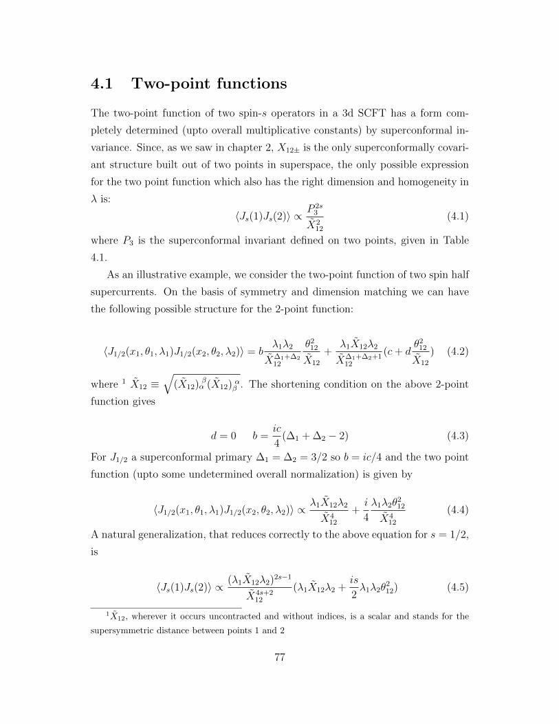
4.1 Two-point functions
The two-point function of two spin-s operators in a 3d SCFT has a form com-
pletely determined (upto overall multiplicative constants) by superconformal in-
variance. Since, as we saw in chapter 2, X12± is the only superconformally covari-
ant structure built out of two points in superspace, the only possible expression
for the two point function which also has the right dimension and homogeneity in
λ is:
〈Js(1)Js(2)〉 ∝ P 2s3
X212
(4.1)
where P3 is the superconformal invariant defined on two points, given in Table
4.1.
As an illustrative example, we consider the two-point function of two spin half
supercurrents. On the basis of symmetry and dimension matching we can have
the following possible structure for the 2-point function:
〈J1/2(x1, θ1, λ1)J1/2(x2, θ2, λ2)〉 = bλ1λ2
X∆1+∆212
θ212
X12
+λ1X12λ2
X∆1+∆2+112
(c+ dθ2
12
X12
) (4.2)
where 1 X12 ≡√
(X12) βα (X12) αβ . The shortening condition on the above 2-point
function gives
d = 0 b =ic
4(∆1 + ∆2 − 2) (4.3)
For J1/2 a superconformal primary ∆1 = ∆2 = 3/2 so b = ic/4 and the two point
function (upto some undetermined overall normalization) is given by
〈J1/2(x1, θ1, λ1)J1/2(x2, θ2, λ2)〉 ∝ λ1X12λ2
X412
+i
4
λ1λ2θ212
X412
(4.4)
A natural generalization, that reduces correctly to the above equation for s = 1/2,
is
〈Js(1)Js(2)〉 ∝ (λ1X12λ2)2s−1
X4s+212
(λ1X12λ2 +is
2λ1λ2θ
212) (4.5)
1X12, wherever it occurs uncontracted and without indices, is a scalar and stands for the
supersymmetric distance between points 1 and 2
77

with 〈J0J0〉 = 1/X212 (since the superconformal shortening condition is different
for spin zero). Note that the above can be written as
〈Js(1)Js(2)〉 ∝(λ1X12λ2 + i
4λ1λ2θ
212)2s
X4s+212
(4.6)
which is the same as (4.1) . The shortening condition on this is satisfied, as may
be explicitly checked.
As a check, we also work out, by elementary field theory methods, the two
point function of the spin 12
current constructed out of the free N = 1 superfield
which is defined as
Φ = φ+ iθψ
Φ = φ+ iθψ∗(4.7)
We find that the 2-point function computed explicitly in the free theory is in
agreement with our result (4.1) above. The spin half supercurrent is
Jα = ΦDαΦ− (DαΦ)Φ (4.8)
Using the equation of motion for Φ this obeys the shortening condition DαJα = 0.
The two point function of two such currents can be obtained after doing Wick
contractions to write 4-point functions in terms of 2-point functions. We use the
free field propagator 〈ΦΦ〉 = 1X12
, and also that,
D1αD2β1
X12
=−i(X12)αβ
(X12)3, D1α
1
X12
D2β1
X12
=εαβθ
212
4(X12)4(4.9)
This gives (upto multiplicative factors which we neglect)
〈Jα(1)Jβ(2)〉 =((−X12)αβ + i
4θ2
12εαβ)
X412
. (4.10)
Contracting with λα1 and λβ2 we find, in free field theory,
〈J 12(1)J 1
2(2)〉 =
P3
X212
(4.11)
which, indeed, is what was expected.
78
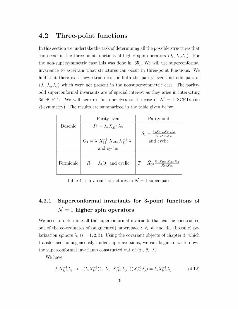
4.2 Three-point functions
In this section we undertake the task of determining all the possible structures that
can occur in the three-point functions of higher spin operators 〈Js1Js2Js3〉. For
the non-supersymmetric case this was done in [35]. We will use superconformal
invariance to ascertain what structures can occur in three-point functions. We
find that there exist new structures for both the parity even and odd part of
〈Js1Js2Js3〉 which were not present in the nonsupersymmetric case. The parity-
odd superconformal invariants are of special interest as they arise in interacting
3d SCFTs. We will here restrict ourselves to the case of N = 1 SCFTs (no
R-symmetry). The results are summarized in the table given below:
Parity even Parity odd
Bosonic P1 = λ2X−123−λ3
S1 = λ3X31+X12+λ2X12X23X31
Q1 = λ1X−112−X23+X
−131−λ1 and cyclic
and cyclic
Fermionic R1 = λ1Θ1 and cyclic T = X31Θ1X12+X23+Θ3
X12X23
Table 4.1: Invariant structures in N = 1 superspace.
4.2.1 Superconformal invariants for 3-point functions of
N = 1 higher spin operators
We need to determine all the superconformal invariants that can be constructed
out of the co-ordinates of (augmented) superspace : xi, θi and the (bosonic) po-
larization spinors λi (i = 1, 2, 3). Using the covariant objects of chapter 3, which
transformed homogeneously under superinversions, we can begin to write down
the superconformal invariants constructed out of (xi, θi, λi).
We have
λiX−1ij−λj → −(λiX
−1i− )(−Xi−X
−1ij−Xj−)(X−1
j+λj) = λiX−1ij−λj (4.12)
79
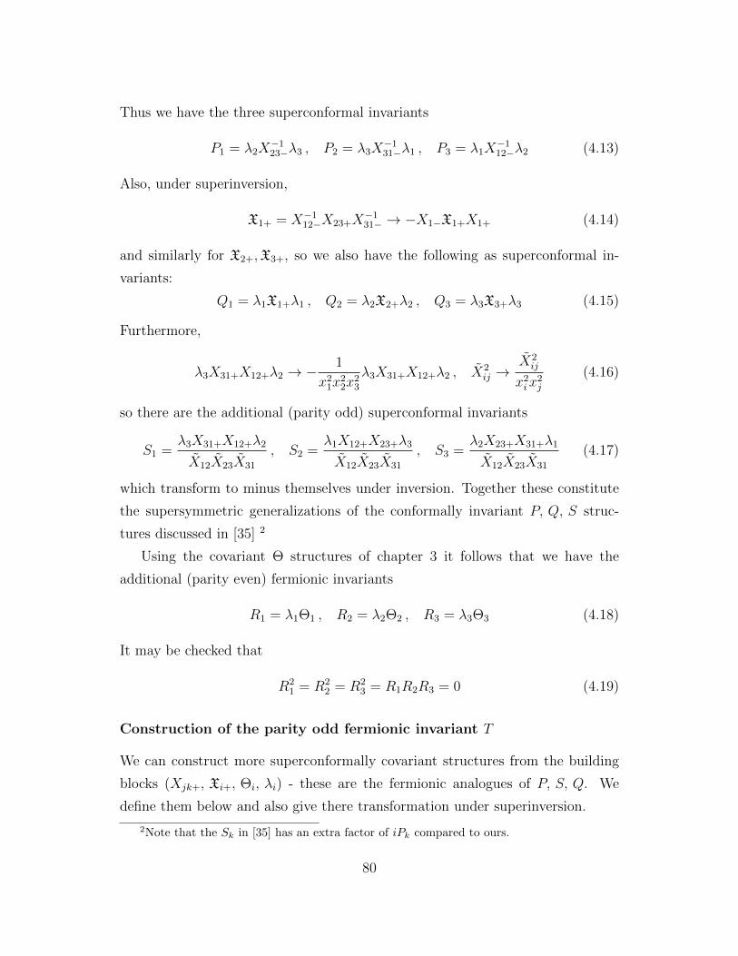
Thus we have the three superconformal invariants
P1 = λ2X−123−λ3 , P2 = λ3X
−131−λ1 , P3 = λ1X
−112−λ2 (4.13)
Also, under superinversion,
X1+ = X−112−X23+X
−131− → −X1−X1+X1+ (4.14)
and similarly for X2+,X3+, so we also have the following as superconformal in-
variants:
Q1 = λ1X1+λ1 , Q2 = λ2X2+λ2 , Q3 = λ3X3+λ3 (4.15)
Furthermore,
λ3X31+X12+λ2 → −1
x21x
22x
23
λ3X31+X12+λ2 , X2ij →
X2ij
x2ix
2j
(4.16)
so there are the additional (parity odd) superconformal invariants
S1 =λ3X31+X12+λ2
X12X23X31
, S2 =λ1X12+X23+λ3
X12X23X31
, S3 =λ2X23+X31+λ1
X12X23X31
(4.17)
which transform to minus themselves under inversion. Together these constitute
the supersymmetric generalizations of the conformally invariant P, Q, S struc-
tures discussed in [35] 2
Using the covariant Θ structures of chapter 3 it follows that we have the
additional (parity even) fermionic invariants
R1 = λ1Θ1 , R2 = λ2Θ2 , R3 = λ3Θ3 (4.18)
It may be checked that
R21 = R2
2 = R23 = R1R2R3 = 0 (4.19)
Construction of the parity odd fermionic invariant T
We can construct more superconformally covariant structures from the building
blocks (Xjk+, Xi+, Θi, λi) - these are the fermionic analogues of P, S, Q. We
define them below and also give there transformation under superinversion.
2Note that the Sk in [35] has an extra factor of iPk compared to ours.
80
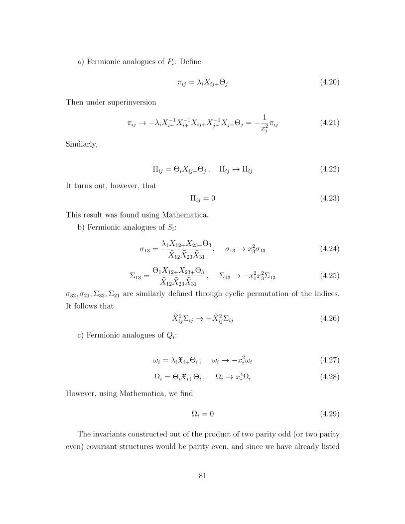
a) Fermionic analogues of Pi: Define
πij = λiXij+Θj (4.20)
Then under superinversion
πij → −λiX−1i−X
−1i+ Xij+X
−1j−Xj−Θj = − 1
x2i
πij (4.21)
Similarly,
Πij = ΘiXij+Θj , Πij → Πij (4.22)
It turns out, however, that
Πij = 0 (4.23)
This result was found using Mathematica.
b) Fermionic analogues of Si:
σ13 =λ1X12+X23+Θ3
X12X23X31
, σ13 → x23σ13 (4.24)
Σ13 =Θ1X12+X23+Θ3
X12X23X31
, Σ13 → −x21x
23Σ13 (4.25)
σ32, σ21,Σ32,Σ21 are similarly defined through cyclic permutation of the indices.
It follows that
X2ijΣij → −X2
ijΣij (4.26)
c) Fermionic analogues of Qi:
ωi = λiXi+Θi , ωi → −x2iωi (4.27)
Ωi = ΘiXi+Θi , Ωi → x4iΩi (4.28)
However, using Mathematica, we find
Ωi = 0 (4.29)
The invariants constructed out of the product of two parity odd (or two parity
even) covariant structures would be parity even, and since we have already listed
81

all the parity even invariants, would be expressible in terms of Pi, Qi, Ri. Thus,
we find the following relations for the above covariant structures
π2ij = σ2
ij = ω2i = 0 (4.30)
πijωi = 0 (4.31)
1
X212
π12π23 = −R1R2 ,1
X223
π23π31 = −R2R3 ,1
X231
π31π12 = −R3R1 (4.32)
1
X2ij
πijπji = RiRj = X2ijσijσji (4.33)
X212σ21σ32 = R2R3 , X2
23σ32σ13 = R3R1 , X231σ13σ21 = R1R2 (4.34)
X2ij ωiωj = −RiRj (4.35)
From the above covariant structures it is possible to build additional parity
odd fermionic invariants by taking products of a parity even and a parity odd
covariant structure.3Thus, we have
Tij = πijσji (4.36)
and under superinversion
Tij → −Tij (4.37)
Note that πij 6= πji so π12, π23, π31 is a different set of parity odd covariant struc-
tures than π21, π32, π13 (the same is true for the even structures σij). However,
because the following relation is true
Tij = −Tji (4.38)
it follows that we have only three odd invariant structures:
T1 ≡ T23 = π23σ32 , T2 ≡ T31 = π31σ13 , T3 ≡ T12 = π12σ21 (4.39)
3Note that structures like xiωi, πij/xi would be parity odd invariants under inversion. How-
ever, these are not Poincare invariant (since correlation functions should depend only on differ-
ences (xij) of the coordinates). We could also construct structures like U = X12X23X31ω1ω2ω3
which would be an odd invariant (U → −U) . However, it is identically zero because the product
of three different Θ’s vanishes.
82
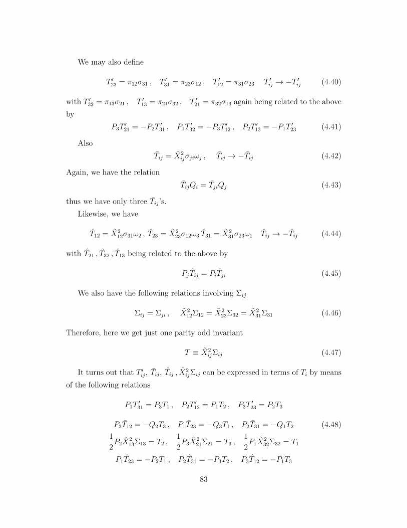
We may also define
T ′23 = π12σ31 , T ′31 = π23σ12 , T ′12 = π31σ23 T ′ij → −T ′ij (4.40)
with T ′32 = π13σ21 , T ′13 = π21σ32 , T ′21 = π32σ13 again being related to the above
by
P3T′21 = −P2T
′31 , P1T
′32 = −P3T
′12 , P2T
′13 = −P1T
′23 (4.41)
Also
Tij = X2ijσjiωj , Tij → −Tij (4.42)
Again, we have the relation
TijQi = TjiQj (4.43)
thus we have only three Tij’s.
Likewise, we have
T12 = X212σ31ω2 , T23 = X2
23σ12ω3 T31 = X231σ23ω1 Tij → −Tij (4.44)
with T21 , T32 , T13 being related to the above by
PjTij = PiTji (4.45)
We also have the following relations involving Σij
Σij = Σji , X212Σ12 = X2
23Σ32 = X231Σ31 (4.46)
Therefore, here we get just one parity odd invariant
T ≡ X2ijΣij (4.47)
It turns out that T ′ij, Tij, Tij , X2ijΣij can be expressed in terms of Ti by means
of the following relations
P1T′31 = P3T1 , P2T
′12 = P1T2 , P3T
′23 = P2T3
P3T12 = −Q2T3 , P1T23 = −Q3T1 , P2T31 = −Q1T2 (4.48)
1
2P2X
213Σ13 = T2 ,
1
2P3X
221Σ21 = T3 ,
1
2P1X
232Σ32 = T1
P1T23 = −P2T1 , P2T31 = −P3T2 , P3T12 = −P1T3
83

Making use of the above equation and eq.(4.47) we can express all parity odd
fermionic structures in terms of T
T2 =1
2P2T , T3 =
1
2P3T , T1 =
1
2P1T (4.49)
T12 = −1
2Q2T , T23 = −1
2Q3T , T31 = −1
2Q1T (4.50)
T ′31 =1
2P3T , T ′12 =
1
2P1T , T ′23 =
1
2P2T (4.51)
T12 = −1
2P1T , T23 = −1
2P2T , T31 = −1
2P3T (4.52)
To summarize, from our fermionic covariant structures we could construct five
parity odd invariants Ti, T′ij, Tij, Tij , T . However, only T suffices as the other
four are related to it through the above simple relations.
We have thus obtained the superconformal invariants Pi, Qi, Ri, Si, T (listed
in tabular form at the beginning of this section) out of which the invariant struc-
tures for particular 3-point functions can be constructed as monomials in these
variables. Before we do this, however, we need to determine all the relations
between these variables using which we can get a linearly independent basis of
monomial structures for 3-point functions.
4.2.2 Relations between the invariant structures
Following [35] we can do a counting of the number of independent (parity even)
invariant structures for 3-point functions in 3d SCFTs with N = 1 supersym-
metry: the superconformal group in this case has 14 generators (10 bosonic, 4
fermionic) and out of (xi, θi, λi) (i = 1, 2, 3, so 7 × 3 real variables) we can con-
struct 7×3−14 = 7 superconformal invariants. Thus among the nine parity even
structures (Pi , Qi , Ri) we must have two relations. One of them is the supersym-
metrized version of the non-linear relation (2.14) in [35]
P 21Q1+P 2
2Q2+P 23Q3−2P1P2P3−Q1Q2Q3−
i
2(R1R2P3Q3+R2R3P1Q1+R3R1P2Q2) = 0
(4.53)
This cuts down the number of independent invariants by one. We also have
the following triplet of relations which vanishes identically when the Grassmann
84
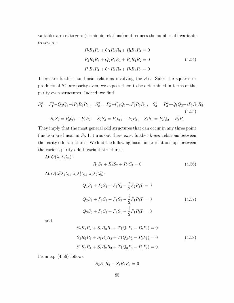
variables are set to zero (fermionic relations) and reduces the number of invariants
to seven :
P2R1R2 +Q1R2R3 + P3R3R1 = 0
P3R2R3 +Q2R3R1 + P1R1R2 = 0 (4.54)
P1R3R1 +Q3R1R2 + P2R2R3 = 0
There are further non-linear relations involving the S’s. Since the squares or
products of S’s are parity even, we expect them to be determined in terms of the
parity even structures. Indeed, we find
S21 = P 2
1−Q2Q3−iP1R2R3 , S22 = P 2
2−Q3Q1−iP2R3R1 , S23 = P 2
3−Q1Q2−iP3R1R2
(4.55)
S1S2 = P3Q3 − P1P2 , S2S3 = P1Q1 − P2P3 , S3S1 = P2Q2 − P3P1
They imply that the most general odd structures that can occur in any three point
function are linear in Si. It turns out there exist further linear relations between
the parity odd structures. We find the following basic linear relationships between
the various parity odd invariant structures:
At O(λ1λ2λ3):
R1S1 +R2S2 +R3S3 = 0 (4.56)
At O(λ21λ2λ3, λ1λ
22λ3, λ1λ2λ
23):
Q1S1 + P2S3 + P3S2 −i
2P2P3T = 0
Q2S2 + P3S1 + P1S3 −i
2P1P3T = 0 (4.57)
Q3S3 + P1S2 + P2S1 −i
2P1P2T = 0
and
S2R1R2 + S3R3R1 + T (Q1P1 − P2P3) = 0
S3R2R3 + S1R1R2 + T (Q2P2 − P3P1) = 0 (4.58)
S1R3R1 + S2R2R3 + T (Q3P3 − P1P2) = 0
From eq. (4.56) follows:
S2R1R2 − S3R3R1 = 0
85
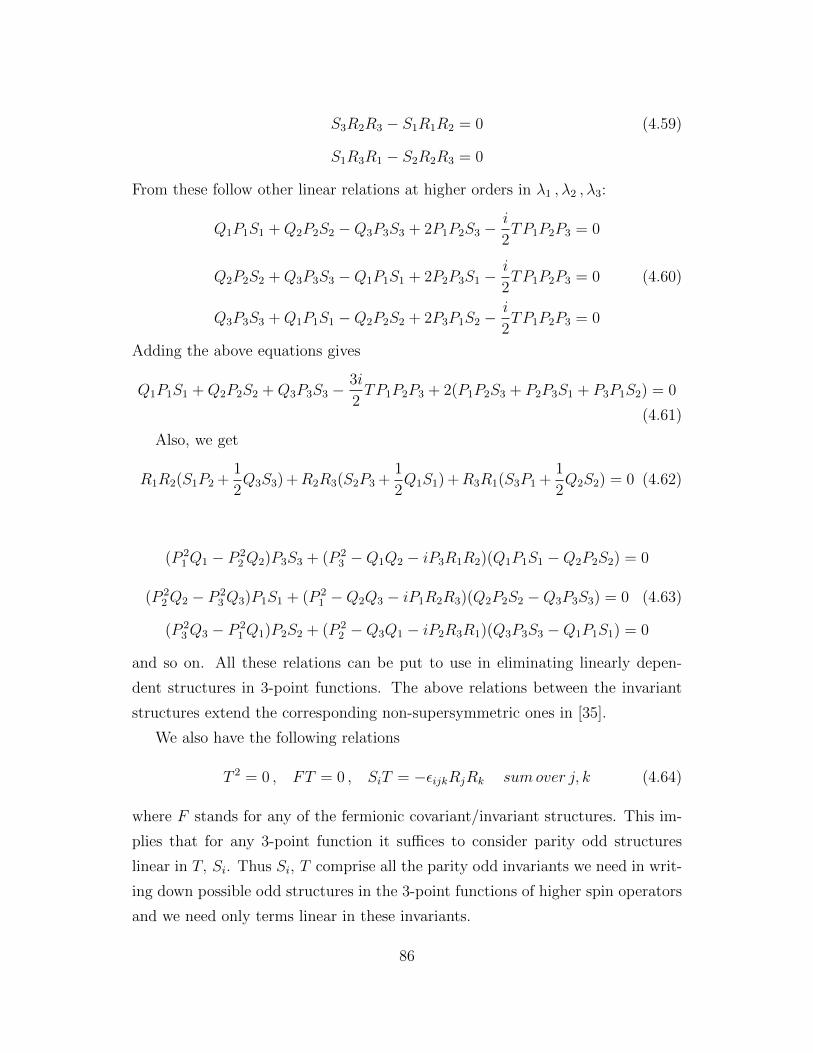
S3R2R3 − S1R1R2 = 0 (4.59)
S1R3R1 − S2R2R3 = 0
From these follow other linear relations at higher orders in λ1 , λ2 , λ3:
Q1P1S1 +Q2P2S2 −Q3P3S3 + 2P1P2S3 −i
2TP1P2P3 = 0
Q2P2S2 +Q3P3S3 −Q1P1S1 + 2P2P3S1 −i
2TP1P2P3 = 0 (4.60)
Q3P3S3 +Q1P1S1 −Q2P2S2 + 2P3P1S2 −i
2TP1P2P3 = 0
Adding the above equations gives
Q1P1S1 +Q2P2S2 +Q3P3S3 −3i
2TP1P2P3 + 2(P1P2S3 + P2P3S1 + P3P1S2) = 0
(4.61)
Also, we get
R1R2(S1P2 +1
2Q3S3) +R2R3(S2P3 +
1
2Q1S1) +R3R1(S3P1 +
1
2Q2S2) = 0 (4.62)
(P 21Q1 − P 2
2Q2)P3S3 + (P 23 −Q1Q2 − iP3R1R2)(Q1P1S1 −Q2P2S2) = 0
(P 22Q2 − P 2
3Q3)P1S1 + (P 21 −Q2Q3 − iP1R2R3)(Q2P2S2 −Q3P3S3) = 0 (4.63)
(P 23Q3 − P 2
1Q1)P2S2 + (P 22 −Q3Q1 − iP2R3R1)(Q3P3S3 −Q1P1S1) = 0
and so on. All these relations can be put to use in eliminating linearly depen-
dent structures in 3-point functions. The above relations between the invariant
structures extend the corresponding non-supersymmetric ones in [35].
We also have the following relations
T 2 = 0 , FT = 0 , SiT = −εijkRjRk sumover j, k (4.64)
where F stands for any of the fermionic covariant/invariant structures. This im-
plies that for any 3-point function it suffices to consider parity odd structures
linear in T, Si. Thus Si, T comprise all the parity odd invariants we need in writ-
ing down possible odd structures in the 3-point functions of higher spin operators
and we need only terms linear in these invariants.
86
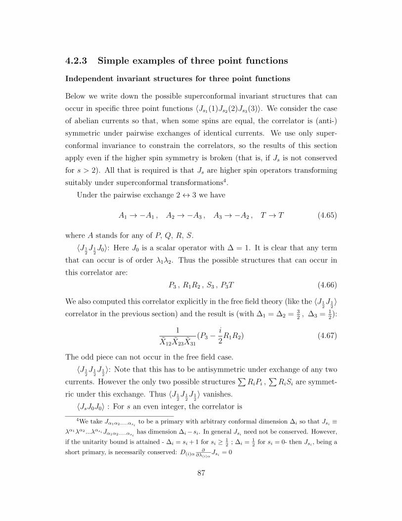
4.2.3 Simple examples of three point functions
Independent invariant structures for three point functions
Below we write down the possible superconformal invariant structures that can
occur in specific three point functions 〈Js1(1)Js2(2)Js3(3)〉. We consider the case
of abelian currents so that, when some spins are equal, the correlator is (anti-)
symmetric under pairwise exchanges of identical currents. We use only super-
conformal invariance to constrain the correlators, so the results of this section
apply even if the higher spin symmetry is broken (that is, if Js is not conserved
for s > 2). All that is required is that Js are higher spin operators transforming
suitably under superconformal transformations4.
Under the pairwise exchange 2↔ 3 we have
A1 → −A1 , A2 → −A3 , A3 → −A2 , T → T (4.65)
where A stands for any of P, Q, R, S.
〈J 12J 1
2J0〉: Here J0 is a scalar operator with ∆ = 1. It is clear that any term
that can occur is of order λ1λ2. Thus the possible structures that can occur in
this correlator are:
P3 , R1R2 , S3 , P3T (4.66)
We also computed this correlator explicitly in the free field theory (like the 〈J 12J 1
2〉
correlator in the previous section) and the result is (with ∆1 = ∆2 = 32, ∆3 = 1
2):
1
X12X23X31
(P3 −i
2R1R2) (4.67)
The odd piece can not occur in the free field case.
〈J 12J 1
2J 1
2〉: Note that this has to be antisymmetric under exchange of any two
currents. However the only two possible structures∑RiPi ,
∑RiSi are symmet-
ric under this exchange. Thus 〈J 12J 1
2J 1
2〉 vanishes.
〈JsJ0J0〉 : For s an even integer, the correlator is
4We take Jα1α2.....αsito be a primary with arbitrary conformal dimension ∆i so that Jsi ≡
λα1λα2 ...λαsiJα1α2.....αsihas dimension ∆i−si. In general Jsi need not be conserved. However,
if the unitarity bound is attained - ∆i = si + 1 for si ≥ 12 ; ∆i = 1
2 for si = 0- then Jsi , being a
short primary, is necessarily conserved: D(i)α∂
∂λ(i)αJsi = 0
87
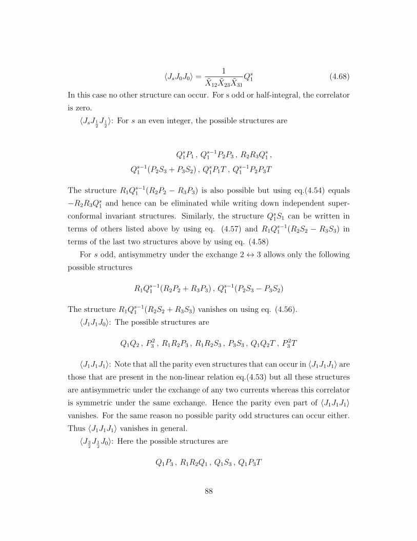
〈JsJ0J0〉 =1
X12X23X31
Qs1 (4.68)
In this case no other structure can occur. For s odd or half-integral, the correlator
is zero.
〈JsJ 12J 1
2〉: For s an even integer, the possible structures are
Qs1P1 , Q
s−11 P2P3 , R2R3Q
s1 ,
Qs−11 (P2S3 + P3S2) , Qs
1P1T , Qs−11 P2P3T
The structure R1Qs−11 (R2P2 − R3P3) is also possible but using eq.(4.54) equals
−R2R3Qs1 and hence can be eliminated while writing down independent super-
conformal invariant structures. Similarly, the structure Qs1S1 can be written in
terms of others listed above by using eq. (4.57) and R1Qs−11 (R2S2 − R3S3) in
terms of the last two structures above by using eq. (4.58)
For s odd, antisymmetry under the exchange 2↔ 3 allows only the following
possible structures
R1Qs−11 (R2P2 +R3P3) , Qs−1
1 (P2S3 − P3S2)
The structure R1Qs−11 (R2S2 +R3S3) vanishes on using eq. (4.56).
〈J1J1J0〉: The possible structures are
Q1Q2 , P23 , R1R2P3 , R1R2S3 , P3S3 , Q1Q2T , P
23 T
〈J1J1J1〉: Note that all the parity even structures that can occur in 〈J1J1J1〉 are
those that are present in the non-linear relation eq.(4.53) but all these structures
are antisymmetric under the exchange of any two currents whereas this correlator
is symmetric under the same exchange. Hence the parity even part of 〈J1J1J1〉vanishes. For the same reason no possible parity odd structures can occur either.
Thus 〈J1J1J1〉 vanishes in general.
〈J 32J 1
2J0〉: Here the possible structures are
Q1P3 , R1R2Q1 , Q1S3 , Q1P3T
88
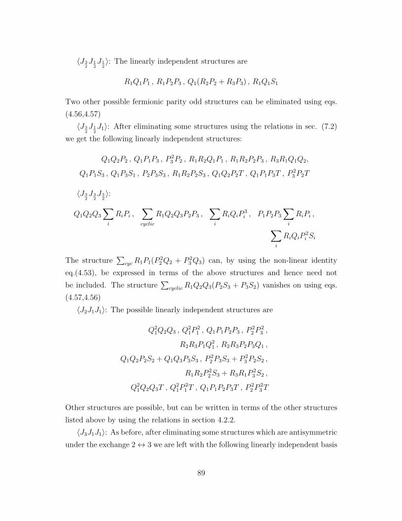
〈J 32J 1
2J 1
2〉: The linearly independent structures are
R1Q1P1 , R1P2P3 , Q1(R2P2 +R3P3) , R1Q1S1
Two other possible fermionic parity odd structures can be eliminated using eqs.
(4.56,4.57)
〈J 32J 1
2J1〉: After eliminating some structures using the relations in sec. (7.2)
we get the following linearly independent structures:
Q1Q2P2 , Q1P1P3 , P23P2 , R1R2Q1P1 , R1R2P2P3 , R3R1Q1Q2,
Q1P1S3 , Q1P3S1 , P2P3S3 , R1R2P2S3 , Q1Q2P2T , Q1P1P3T , P23P2T
〈J 32J 3
2J 3
2〉:
Q1Q2Q3
∑i
RiPi ,∑cyclic
R1Q2Q3P2P3 ,∑i
RiQiP3i , P1P2P3
∑i
RiPi ,∑i
RiQiP2i Si
The structure∑
cycR1P1(P 22Q2 + P 2
3Q3) can, by using the non-linear identity
eq.(4.53), be expressed in terms of the above structures and hence need not
be included. The structure∑
cyclicR1Q2Q3(P2S3 + P3S2) vanishes on using eqs.
(4.57,4.56)
〈J2J1J1〉: The possible linearly independent structures are
Q21Q2Q3 , Q
21P
21 , Q1P1P2P3 , P
22P
23 ,
R2R3P1Q21 , R2R3P2P3Q1 ,
Q1Q2P2S2 +Q1Q3P3S3 , P22P3S3 + P 2
3P2S2 ,
R1R2P22S3 +R3R1P
23S2 ,
Q21Q2Q3T , Q
21P
21 T , Q1P1P2P3T , P
22P
23 T
Other structures are possible, but can be written in terms of the other structures
listed above by using the relations in section 4.2.2.
〈J3J1J1〉: As before, after eliminating some structures which are antisymmetric
under the exchange 2↔ 3 we are left with the following linearly independent basis
89
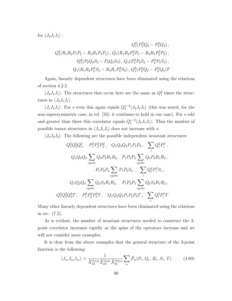
for 〈J3J1J1〉 :
Q21(P 2
2Q2 − P 23Q3) ,
Q21(R1R2P1P2 −R3R1P3P1) , Q1(R1R2P
22P3 −R3R1P
23P2) ,
Q21(P2Q2S2 − P3Q3S3) , Q1(P 2
3P2S2 − P 22P3S3) ,
Q1(R1R2P22S3 −R3R1P
23S2) , Q2
1(P 22Q2 − P 2
3Q3)T
Again, linearly dependent structures have been eliminated using the relations
of section 4.2.2.
〈J4J1J1〉: The structures that occur here are the same as Q21 times the struc-
tures in 〈J2J1J1〉.〈JsJ1J1〉: For s even this again equals Qs−2
1 〈J2J1J1〉 (this was noted, for the
non-supersymmetric case, in ref. [35]- it continues to hold in our case). For s odd
and greater than three this correlator equals Qs−21 〈J3J1J1〉. Thus the number of
possible tensor structures in 〈JsJ1J1〉 does not increase with s.
〈J2J2J2〉: The following are the possible independent invariant structures
Q21Q
22Q
23 , P 2
1P22P
23 , Q1Q2Q3P1P2P3 ,
∑i
Q2iP
4i ,
Q1Q2Q3
∑cyclic
Q3P3R1R2 , P1P2P3
∑cyclic
Q3P3R1R2 ,
P1P2P3
∑cyclic
P1P2S3 ,∑i
Q2iP
3i Si ,
Q1Q2Q3
∑cyclic
Q3S3R1R2 , P1P2P3
∑cyclic
Q3S3R1R2 ,
Q21Q
22Q
23T , P 2
1P22P
23 T , Q1Q2Q3P1P2P3T ,
∑i
Q2iP
4i T
Many other linearly dependent structures have been eliminated using the relations
in sec. (7.2).
As is evident, the number of invariant structures needed to construct the 3-
point correlator increases rapidly as the spins of the operators increase and we
will not consider more examples.
It is clear from the above examples that the general structure of the 3-point
function is the following:
〈Js1Js2Js3〉 =1
Xm12312 Xm231
23 Xm31231
∑n
Fn(Pi, Qi, Ri, Si, T ) (4.69)
90

where mijk ≡ (∆i − si) + (∆j − sj) − (∆k − sk) and the sum is over all the
independent invariant structures Fn, each of homogeneity λ2s11 λ2s2
2 λ2s33 . Since the
3-point function is linear in the parity odd invariants and linear or bilinear in the
R’s (either Ri or RjRk , j 6= k), we have the following structure for Fn:
Fn = F (1)n (Pi, Qi) + a(1)
n F (1)n (Pi, Qi)T + a(2)
n F (2)n (Pi, Qi)Si + a(3)
n F (3)n (Pi, Qi)Ri
+a(4)n F (4)
n (Pi, Qi)RiSj + a(5)n F (5)
n (Pi, Qi)RjRk + a(6)n F (6)
n (Pi, Qi)RjRkSl
Here each F(a)n (Pi, Qi) is a monomial in P ’s and Q’s such that each term on the
r.h.s above has homogeneity λ2s11 λ2s2
2 λ2s33 .5
Three point functions of conserved currents
We have so far considered the constraints on the structure of the three-point
functions of higher spin operators arising due to superconformal invariance alone.
We will now see how the structure is further constrained by current conservation,
i.e, when the operators are actually conserved higher spin currents. In this section
we present evidence for the claim that the three point function of the conserved
higher spin currents in N = 1 superconformal field theory consists of two linearly
independent parts, i.e.,
〈Js1Js2Js3〉 =1
X12X23X31
(a〈Js1Js2Js3〉even + b〈Js1Js2Js3〉odd
)(4.70)
where a and b are independent constants, and the ‘even’ structure arises from free
field theory.
The procedure, quite similar to that used by [35], is as follows. For any par-
ticular three point function we first consider the linearly independent basis of
monomial structures (listed in section 4.2.3) and take an arbitrary linear combi-
nation of these structures.
〈Js1Js2Js3〉 =1
X12X23X31
∑n
anFn (4.71)
5The six F(a)n (Pi, Qi) are not independent functions. F
(2)n , F
(4)n , F
(6)n can be obtained from
F(1)n , F
(3)n , F
(5)n , respectively, by replacing a P pi in the latter by P p−1
i Si (suitably (anti-) sym-
metrized if some spins are equal in the 3-point function)
91

Current conservation Dα1Jα1α2.....α2s = 0 is tantamount to the following equa-
tion on the contracted current Js(x, λ) :
Dα∂
∂λαJs = 0 (4.72)
Thus the equation
Di∂
∂λi〈Js1Js2Js3〉 = 0 (4.73)
for each i = 1, 2, 3 gives additional constraints in the form of linear equations in the
an’s- some of these constants can thus be determined. The algebraic manipulations
get quite unwieldy- we used superconformal invariance to set some co-ordinates
to particular values and took recourse to Mathematica6. The results obtained are
given below (the known Xij dependent factors in the denominator are not listed
below):
Three-pt function Even Odd
〈J 12J 1
2J0〉 P3 − i
2R1R2 S3 − i
2P3T
〈J1J 12J0〉 P3R1 + 1
2Q1R2 0
〈J1J1J0〉 12Q1Q2 + P 2
3 − iR1R2P3 S3P3 + i2(S3R1R2 −Q1Q2T )
〈J 32J 1
2J0〉 P3Q1 − i
2Q1R1R2 Q1S3 − iQ1P3T
〈J 32J 1
2J 1
2〉 Q1R1P1 +Q1(R2P2 +R3P3) + 2R1P2P3 0
〈J2J 12J 1
2〉 Q2
1P1 − 4Q1P2P3 − 5i2R2R3Q
21 Q1(P2S3 + P3S2)
+ i2(Q2
1P1 − 3Q1P2P3)T
Table 4.2: Explicit examples of conserved three-point functions.
Using expression (3.33) for the currents in the N = 1 free theory, some 3-point
functions were explicitly evaluated (again using Mathematica, as the computations
get quite cumbersome beyond a few lower spin examples). It must be emphasized
that the (tabulated) even structures obtained above match with the expressions
obtained from free field theory (upto overall constants). We thus have some
evidence for the claim that the three-point function of conserved currents has a
parity even part (generated by a free field theory) and a parity odd piece.
6We would like to acknowledge the use of Matthew Headrick’s grassmann Mathematica
package for doing computations with fermionic variables.
92

Chapter 5
Summary and Outlook
In this chapter we summarise the results presented in chapters 2, 3 and 4 and give
a brief overview of some possible directions for future work. To begin with, in
Chapter 2, we first examined solutions to higher-dimensional field equations for
geometries of the form of eq. (2.1), with maximal symmetry in the noncompact
dimensions. We asked what features of a solution control the curvature in the
maximally symmetric, noncompact dimensions. We discussed no-go theorems on
obtaining dS compactifications in supergravity theories and considered the effects
of bulk singularities, backreacting brane sources and space-filling fluxes on the
lower dimensional curvature of the solution.
Our main result is given by eq. (2.17), which gives the noncompact curvature
scalar as a sum of four terms: R ∝ I + II + III + IV . Here I corresponds to
the bulk action evaluated at the appropriate back-reacted solution; II denotes an
integral over a total derivative involving the warp factor (whose sign is usually
definite, and not de Sitter-like); III denotes the direct contribution of the actions
of any localized sources; and IV denotes a term which vanishes for solutions
that are maximally symmetric in the non-compact dimensions, in the absence of
space-filling fluxes.
We showed that the (classical) cosmological constant of the d dimensional
spacetime is related, under quite general assumptions, to the asymptotic form
of the bulk fields in the near boundary/source limit- we need not know the full
bulk profile the solution. The boundary data includes contributions from the
93

on-shell action, warping effects and the source action. Thus understanding the
backreaction of the localised objects that source the bulk fields is crucial in looking
for classical de Sitter solutions.
Eq. (2.17) relates the curvature to the on-shell bulk action. Remarkably, it
is very often true that this on-shell action is also a total derivative. A sufficient
condition for this turns out to be the existence of a scale invariance of the classical
equations of motion [67], which in particular is present for most higher-dimensional
supergravity theories of general interest. When Son−shell is the integral of a total
derivative, the curvature of the noncompact dimensions is completely determined
by the asymptotic form of a particular combination of bulk fields near any sources
that are distributed around the extra dimensions.
These arguments have two main implications. First, they show (at least for
codimension-two sources) that source back-reaction and the source actions cannot
be neglected when seeking de Sitter solutions. But they also show that all of the
details of the complete back-reacted solution are not required; it often suffices to
know the asymptotic behaviour of the bulk fields in the near-source limit. We
explicitly derive which bulk fields play this role for 11D supergravity and 10D
Type IIA and Type IIB supergravity.
We also demonstrated that all solutions (warped or unwarped) of the metric-
axio-dilaton theory with only codimension two sources are d-dimensional flat. This
generalises the known F theory result for unwarped solutions. This result is true
because the boundary conditions that must be satisfied near the sources relate the
near-source asymptotics of the bulk fields in such a way that the contributions II
and III precisely cancel. We can look at more general solutions with higher form
fluxes and higher codimension branes in the hope of obtaining dS.
Subsequent work [74] based on the results presented in [40] (and discussed in
chapter 2) deals in particular with the application of these methods to type II
supergravity flux compactifications. In such solutions it was investigated further
how the classical cosmological constant is fully determined by the boundary con-
ditions of the fields in the near-source region. The implications for meta-stable
de Sitter solutions in IIB theory, obtained by placing anti-D3 branes at the tip of
a warped Klebanov-Strassler geometry [72], were considered. A topological argu-
94
ment was presented which demonstrates the presence of a singularity in the flux
energy density of the backreacted solution.
Also, classical de Sitter solutions in higher (d > 4) dimensions were considered
by [75]. It was shown here that orientifold compactifications of type II supergrav-
ity theories to d dimensions can not give rise to meta-stable de Sitter solutions for
d > 6. There are only a few possibilities in d = 5, 6 and they all require negative
tension orientifold planes and negative curvature compact manifolds, as discussed
in section 2.2
Besides potentially addressing issues of dark energy and inflation in cosmology
a natural de Sitter embedding in supergravity/string theory would also help in
gaining a more complete understanding of holography for dS gravity.
In chapter 3 we embarked on the study of 3d superconformal theories in an
on-shell superspace formalism. We summarize the main results obtained in this
regard, and presented in chapters 3 and 4, below:
• Classification of superconformal invariants formed out of 3 polarization
spinors and 3 superspace points (following [36]) and using it to constrain
3 point functions of higher spin operators in 3d superconformal field theo-
ries in section 4.2.1.
• A conjecture - and evidence - that there are exactly two structure allowed
in the 3 point functions of the conserved higher spin currents for N = 1 in
section 4.2.3.
• An explicit construction of higher spin conserved current supermultiplets in
terms of on shell elementary superfields in free superconformal field theories
in section 3.2.2.
• The superspace structure of higher spin symmetry breaking on adding in-
teractions to large N gauge theories in section 3.3.
The 3-point functions of higher spin operator supermultiplets were constructed
in terms of superconformal invariants built out of superspace co-ordinates and
bosonic polarization spinors. For this purpose, following earlier work of Hugh
95
Osborn and J.H. Park , we constructed the various parity even and odd super-
conformal invariant structures out of the covariant structures which superspace
admits.
The myriad non-linear relations between these invariants were discovered (this
required extensive manipulations of grasmannian variables on Mathematica). This
enabled the determination of a basis of linearly independent monomial structures
(built out of the invariants) for the possible structures which can occur in 3-point
functions of higher spin operators. Thus the form of the 3-point functions was
constrained on the basis of superconformal invariance alone.
Thereafter, the constraints arising from imposition of conservation of currents
of higher spin were considered. It was conjectured, and evidence through examples
was provided, that the 3-point function of conserved higher spin currents is the
sum of a parity even and a parity odd part with the parity even piece arising from
free SCFTs. This 3-point function analysis extended the earlier work of Giombi,
Prakash and Yin [35].
It should be possible to build on this line of work in some different, but related,
directions:
• Extending the 3-point function analysis to SCFTs with R-symmetry (i.e.
with extended supersymmetry). Several interesting theories which are cur-
rently being studied intensively are of this class.
• The analysis can also be extended to higher dimensions - for four and six
dimensional SCFTs. The superconformal covariant structures in four and
six dimensions are known [37, 38]. We may also note here that for d >
3 CFTs it is known that the invariants are all independent and so there
are no complicated non-linear relationships between them which need to
determined prior to writing down the structures for 3-point functions. Also
there is only one parity odd invariant in d = 4 and none in d = 6, so the
analysis may be considerably simpler.
• Extending the various recent results of Maldacena and Zhiboedov on CFTs
[32] with weakly broken higher spin symmetry. In SCFTs with weakly bro-
ken higher spin symmetry (eg. Chern-Simons SCFTs) the superspace struc-
96
ture of the anomalous ”conservation” equation is more constrained (see sec-
tion 3.3) and this presumably can be used profitably to constrain correlators
to a greater degree.
• 3d SCFTs with higher spin operators include a range of theories describ-
ing a variety of Renormalization group fixed points. In particular they
include Large N supersymmetric Chern-Simons theories with vector matter
(i.e. with matter fields, bosonic/fermionic, transforming in the fundamental
representation of the gauge group) or bi-fundamental matter (such as ABJ
theory) which are currently an active avenue of research. This includes de-
termining the single-trace operator spectrum, the exact large N solution of
various such theories on different 3-manifolds by computing the partition
function and their phase structure at finite temperature.
• 3d SCFTs are expected to be holographically dual to 4-dimensional theories
of gravity (via the AdS/CFT duality map). In particular, field theories with
higher spin operators are expected to be dual to Vasiliev type theories of
massless higher spins in AdS spacetime. Thus, insight into the complicated
non-linear dynamics of these theories (which themselves describe string the-
ory in the highly stringy tensionless limit) can be obtained by studying such
CFTs.
• Extending the analysis of 3-point functions to 4 and higher point functions
in view of implementing the (super) conformal bootstrap for higher spin op-
erators. This has been implemented mainly for scalar operators, but it may
be possible to take forward some of this work using the formalism devel-
oped in chapter 4 by using polarisation spinor and superspace techniques,
perhaps together with the embedding formalism for CFTs ([44, 45], see also
[42, 43]).
It would be interesting to work on this range of topics in the future as they
would shed light on the dynamics of a variety of CFTs. One may hope for the exact
solution of vector model CFTs (at least in the large N limit) and the application
of bootstrap methods to learn more about CFTs in general, in various dimensions.
97
Bibliography
[1] G. W. Gibbons and S. W. Hawking, “Cosmological event horizons, thermo-
dynamics, and particle creation,” Phys. Rev. D 15 (1977) 2738.
[2] W. Fischler, “Taking de Sitter seriously”, talk given at Role of Scaling Laws
in Physics and Biology (Celebrating the 60th Birthday of G. West), Santa
Fe, December 2000.
[3] T. Banks, “Cosmological breaking of supersymmetry or little Lambda goes
back to the future. II,” arXiv:hep-th/0007146
[4] E. Witten, “Quantum gravity in de Sitter space,” arXiv:hep-th/0106109.
[5] A. Strominger, “The dS/CFT correspondence,” JHEP 0110 (2001) 034
[arXiv:hep-th/0106113]
[6] C.M. Hull, “Timelike T-duality, de Sitter space, large N gauge theories and
topological field theory,” JHEP 9807 (1998) 021 [arXiv:hep-th/9806146].
[7] G. W. Gibbons, “Aspects of supergravity theories,” in Supergravity and re-
lated topics, eds. F. de Aguila, J.A. de Azcaarraga and L. Ibanez, (World
scientific, 1985)
[8] J. Maldacena and C. Nunez, “Supergravity description of field theories on
curved manifolds and a no go theorem,” Int. J. Mod. Phys. A 16 (2001) 822,
[arXiv:hep-th/0007018]
[9] G.W. Gibbons and C. M. Hull, “De Sitter space from warped supergravity
solutions,” arXiv:hep-th/0111072.
98

[10] P. K. Townsend and M. N. R. Wohlfarth, “Accelerating cosmologies from
compactification,” Phys. Rev. Lett. 91, 061302 (2003) [arXiv:hep-th/0303097]
[11] P. K. Townsend, “Cosmic acceleration and M-theory” (2003) Arxiv: hep-
th/0308149
[12] E. Silverstein, “Simple de Sitter Solutions” Phys. Rev. D 77, 106006 (2008)
[Arxiv: hep-th/0712.1196]
[13] M. Douglas and R. Kallosh, “Compactification on negatively curved mani-
folds” Arxiv: hep-th/1001.4008
[14] A.J.Tolley,C.P.Burgess, D. Hoover and Y. Aghababaie “Bulk singularities
and the effective cosmological constant for higher co-dimension branes”,
JHEP03(2006)091 [Arxiv: hep-th/0512218]
[15] D. H. Wesley, “New no-go theorems for cosmic acceleration with extra di-
mensions” [arXiv:hep-th/0802.2106]
[16] D. H. Wesley, “Oxidised cosmic acceleration”, JCAP 0901, 041 (2009)
[arXiv:hep-th/0802.3214 ]
[17] P. J. Steinhardt and D. Wesley, “Dark Energy, Inflation and Extra Dimen-
sions”, Phys. Rev. D 79, 104026 (2009) [arXiv:hep-th/0811.1614].
[18] A. Bayntun, C. P. Burgess, L. van Nierop, “Codimension-2 Brane-Bulk
Matching: Examples from Six and Ten Dimensions,” New J. Phys. 12 (2010)
075015. [arXiv:0912.3039 [hep-th]].
[19] B. R. Greene, A. D. Shapere, C. Vafa and S. T. Yau, “Stringy Cosmic Strings
And Noncompact Calabi-Yau Manifolds,” Nucl. Phys. B 337 (1990) 1.
[20] J. Maldacena, “The Large N limit of superconformal field theories and
supergravity”, Adv.Theor.Math.Phys., vol.2, 231-252 (1998) [arXiv:hep-
th/9711200]
[21] E. Witten, “Anti-de Sitter space and holography,” Adv.Theor.Math.Phys.2
(1998) 253-291, arXiv:hep-th/9802150
99
[22] S. S. Gubser, I. R. Klebanov, and A. M. Polyakov, “Gauge theory correlators
from non-critical string theory,” Phys. Lett. B428 (1998) 105-114, arXiv:hep-
th/9802109.
[23] A. Belavin, A. M. Polyakov, and A. Zamolodchikov, “Infinite Conformal
Symmetry in Two-Dimensional Quantum Field Theory,” Nucl.Phys. B241
(1984) 333-380.
[24] I. Klebanov and A. Polyakov, “AdS dual of the critical O(N) vector model,”
Phys.Lett. B550 (2002) 213-219, arXiv:hep-th/0210114
[25] E. Sezgin and P. Sundell, “Holography in 4D (super) higher spin theories and
a test via cubic scalar couplings,” JHEP 07 (2005) 044, arXiv:hep-th/0305040
[26] O. Aharony, G. Gur-Ari, and R. Yacoby, “d=3 Bosonic Vector Mod-
els Coupled to Chern-Simons Gauge Theories,”JHEP 1203 (2012) 037,
arXiv:1110.4382 [hep-th]
[27] S. Giombi, S. Minwalla, S. Prakash, S. P. Trivedi, S. R. Wadia, X.
Yin, “Chern-Simons Theory with Vector Fermion Matter,” arXiv:hep-
th/1110.4386
[28] O. Aharony, O. Bergman, D. L. Jafferis, J. Maldacena, “N=6 superconformal
Chern-Simons-matter theories, M2-branes and their gravity duals,” JHEP
0810, 091 (2008). [arXiv:0806.1218 [hep-th]].
O. Aharony, O. Bergman, D. L. Jafferis, “Fractional M2-branes,” JHEP 0811,
043 (2008). [arXiv:0807.4924 [hep-th]].
[29] C.-M. Chang, S. Minwalla, T. Sharma, and X. Yin, “ABJ Triality: from
Higher Spin Fields to Strings,” arXiv:1207.4485 [hep-th]
[30] S. Jain, S. P. Trivedi, S. R. Wadia, and S. Yokoyama, “Supersymmetric
Chern-Simons Theories with Vector Matter,” arXiv:1207.4750 [hep-th]
[31] J. Maldacena and A. Zhiboedov, “Constraining Conformal Field Theories
with A Higher Spin Symmetry”, (2011) [arXiv:hep-th/1112.1016]
100

[32] J. Maldacena and A. Zhiboedov, “Constraining Conformal Field Theo-
ries with a slightly broken Higher Spin Symmetry”, (2012) [arXiv:hep-
th/1204.3882]
[33] I. Heemskerk, J. Penedones, J. Polchinski, and J. Sully, “Holography from
Conformal Field Theory”, JHEP 10 (2009) 079 , arXiv:0907.0151 [hep-th]
[34] A.Liam Fitzpatrick , Jared Kaplan, “AdS Field Theory from Conformal Field
Theory”, JHEP 1302 (2013) 054 arXiv:1208.0337 [hep-th]
[35] S. Giombi, S. Prakash and Xi Yin, “A Note on CFT Correlators in Three
Dimensions”, (2011) [arXiv:hep-th/1104.4317]
[36] J. H. Park, “Superconformal symmetry in three-dimensions”, J.Math.Phys.,
vol. 41,7129-7161 (2000) [arXiv:hep-th/9910199]
[37] H. Osborn, “N=1 superconformal symmetry in four-dimensional quantum
field theory”, Annals Phys., vol.272, 243-294 (1999) [arXiv:hep-th/9808041]
[38] J. H. Park, “N=1 superconformal symmetry in four-dimensions”,
Int.J.Mod.Phys. , vol. A13, 1743-1772 (1998) [arXiv:hep-th/9703191]
J. H. Park, “Superconformal symmetry and correlation functions, Nucl.Phys.,
B559, 455-501 (1999) [arXiv:hep-th/9903230]
J. H. Park, “Superconformal symmetry in six-dimensions and its reduction to
four-dimensions”, Nucl.Phys., B539, 599-642 (1999) [arXiv:hep-th/9807186]
[39] M. A. Vasiliev, “More On Equations Of Motion For Interacting Massless
Fields Of All Spins In (3+1)-Dimensions,” Phys. Lett. B 285, 225 (1992);
M. A. Vasiliev, “Higher-spin gauge theories in four, three and two dimen-
sions,” Int. J. Mod. Phys. D 5, 763 (1996) [arXiv:hep-th/9611024];
M. A. Vasiliev, “Higher spin gauge theories: Star-product and AdS space,”
arXiv:hep-th/9910096; M. A. Vasiliev, “Nonlinear equations for symmet-
ric massless higher spin fields in (A)dS(d),” Phys. Lett. B 567, 139 (2003)
[arXiv:hep-th/0304049].
101
[40] C.P. Burgess, A. Maharana, L. Van Nierop, Amin A. Nizami, F. Quevedo,
“On Brane Back-Reaction and de Sitter Solutions in Higher-Dimensional
Supergravity”, JHEP 1204 (2012) 018, arXiv:1109.0532 [hep-th].
[41] Amin A. Nizami, Tarun Sharma and V. Umesh, “Superspace formulation and
correlation functions of 3d superconformal field theories”, arXiv:1308.4778
[hep-th].
[42] M. S. Costa, J. Penedones, D. Poland, and S. Rychkov, “Spinning Conformal
Blocks,” arXiv:1109.6321 [hep-th].
[43] M. S. Costa, J. Penedones, D. Poland, and S. Rychkov, “Spinning Conformal
Correlators,” arXiv:1107.3554 [hep-th]
[44] P. A.M. Dirac, “Wave equations in conformal space,” Annals Math. 37 (1936)
429-442.
[45] S. Weinberg, “Six-dimensional Methods for Four-dimensional Conformal
Field Theories,” Phys.Rev. D82 (2010) 045031, arXiv:1006.3480 [hep-th]
[46] S. Weinberg, Phys. Lett. 9, 357 (1964); Phys. Rev. 135, B1049 (1964);
Phys.Rev. 140, B515(1965).
[47] S. M. Carroll and M. M. Guica, “Sidestepping the cosmological constant with
football-shaped extra dimensions,” arXiv:hep-th/0302067;
Y. Aghababaie, C. P. Burgess, S. L. Parameswaran, F. Quevedo, “SUSY
breaking and moduli stabilization from fluxes in gauged 6-D supergravity,”
JHEP 0303 (2003) 032 [hep-th/0212091]; “Towards a naturally small cosmo-
logical constant from branes in 6-D supergravity,” Nucl. Phys. B680 (2004)
389-414. [hep-th/0304256].
[48] A. J. Tolley, C. P. Burgess, D. Hoover, Y. Aghababaie, “Bulk singularities and
the effective cosmological constant for higher co-dimension branes,” JHEP
0603 (2006) 091. [hep-th/0512218].
102
[49] G.W. Gibbons, in F. del Aguila, J.A. de Azcarraga, L.E. Ibanez (eds), ”Su-
persymmetry, supergravity and related topics”. World Scientific, Singapore
(1985).
[50] J. Maldacena and C. Nunez, “Supergravity description of field theories on
curved manifolds and a no go theorem,” Int. J. Mod. Phys. A16 (2001)
822-855 [arXiv:hep-th/0007018].
[51] D. H. Wesley, “Oxidised cosmic acceleration,” JCAP 0901 (2009) 041,
[arXiv:0802.3214 [hep-th]].
[52] P.J. Steinhardt and D. Wesley, “Dark Energy, Inflation and Extra Dimen-
sions,” Phys. Rev. D79 104026 (2009).
[53] S. Kachru, R. Kallosh, A. D. Linde, S. P. Trivedi, “De Sitter vacua in string
theory,” Phys. Rev. D68 (2003) 046005. [hep-th/0301240];
C. P. Burgess, R. Kallosh, F. Quevedo, “De Sitter string vacua from super-
symmetric D terms,” JHEP 0310 (2003) 056. [hep-th/0309187];
D. Cremades, M. -P. Garcia del Moral, F. Quevedo, K. Suruliz, “Moduli
stabilisation and de Sitter string vacua from magnetised D7 branes,” JHEP
0705 (2007) 100. [hep-th/0701154];
S. Krippendorf, F. Quevedo, “Metastable SUSY Breaking, de Sitter Mod-
uli Stabilisation and Kahler Moduli Inflation,” JHEP 0911 (2009) 039.
[arXiv:0901.0683 [hep-th]].
[54] E. Silverstein, “Simple de Sitter Solutions,” Phys. Rev. D77 (2008) 106006.
[arXiv:0712.1196 [hep-th]];
S. S. Haque, G. Shiu, B. Underwood, T. Van Riet, “Minimal simple de Sitter
solutions,” Phys. Rev. D79 (2009) 086005. [arXiv:0810.5328 [hep-th]];
T. Wrase, M. Zagermann, “On Classical de Sitter Vacua in String Theory,”
Fortsch. Phys. 58 (2010) 906-910. [arXiv:1003.0029 [hep-th]];
U. H. Danielsson, P. Koerber, T. Van Riet, “Universal de Sitter solutions at
tree-level,” JHEP 1005 (2010) 090. [arXiv:1003.3590 [hep-th]];
103
U. H. Danielsson, S. S. Haque, P. Koerber, G. Shiu, T. Van Riet, T. Wrase,
“De Sitter hunting in a classical landscape,” Fortsch. Phys. 59 (2011) 897-
933. [arXiv:1103.4858 [hep-th]];
G. Shiu, Y. Sumitomo, “Stability Constraints on Classical de Sitter Vacua,”
[arXiv:1107.2925 [hep-th]].
[55] S. Weinberg, Gravitation and Cosmology, John Wiley & Sons 1972.
[56] C. W. Misner, K. S. Thorne, and J. A. Wheeler, Gravitation, W. H. Freeman
and Company 1973.
[57] H. Nishino and E. Sezgin, Phys. Lett. 144B (1984) 187; “The Complete N=2,
D = 6 Supergravity With Matter And Yang-Mills Couplings,” Nucl. Phys.
B278 (1986) 353;
S. Randjbar-Daemi, A. Salam, E. Sezgin and J. Strathdee, “An Anomaly
Free Model in Six-Dimensions” Phys. Lett. B151 (1985) 351.
[58] K. Lanczos, Phys. Z. 23 (1922) 239–543; Ann. Phys. 74 (1924) 518–540;
C.W. Misner and D.H. Sharp, “Relativistic Equations for Adiabatic, Spher-
ically Symmetric Gravitational Collapse” Phys. Rev. 136 (1964) 571–576;
W. Israel, “Singular hypersurfaces and thin shells in general relativity” Nuov.
Cim. 44B (1966) 1–14; errata Nuov. Cim. 48B 463.
[59] L. Randall, R. Sundrum, ”A Large Mass Hierarchy from a Small Extra Di-
mension” Phys. Rev. Lett. 83 (1999) 3370 [hep-ph/9905221]; Phys. Rev.
Lett. 83 (1999) 4690 [hep-th/9906064].
[60] W. D. Goldberger, M. B. Wise, “Renormalization group flows for brane cou-
plings,” Phys. Rev. D65 (2002) 025011 [hep-th/0104170];
E. Dudas, C. Papineau, V.A. Rubakov, “Flowing to four dimensions”
JHEP0603:085,2006 arXiv:hep-th/0512276v1;
C. de Rham, “The Effective Field Theory of Codimension-two Branes,” JHEP
0801 (2008) 060 [arXiv:0707.0884 [hep-th]];
104
C. P. Burgess, C. de Rham, L. van Nierop, “The Hierarchy Problem and the
Self-Localized Higgs,” JHEP 0808 (2008) 061. [arXiv:0802.4221 [hep-ph]].
[61] C. P. Burgess, D. Hoover, G. Tasinato, “UV Caps and Modulus Stabi-
lization for 6D Gauged Chiral Supergravity,” JHEP 0709 (2007) 124.
[arXiv:0705.3212 [hep-th]];
C. P. Burgess, D. Hoover, C. de Rham, G. Tasinato, “Effective Field The-
ories and Matching for Codimension-2 Branes,” JHEP 0903 (2009) 124.
[arXiv:0812.3820 [hep-th]].
[62] P. Bostock, R. Gregory, I. Navarro and J. Santiago, “Einstein gravity on
the codimension 2 brane?,” Phys. Rev. Lett. 92 (2004) 221601 [arXiv:hep-
th/0311074];
J. Vinet and J. M. Cline, “Codimension-two branes in six-dimensional su-
pergravity and the cosmological constant problem,” Phys. Rev. D 71 (2005)
064011 [hep-th/0501098];
M. Peloso, L. Sorbo and G. Tasinato, “Standard 4d gravity on a brane
in six dimensional flux compactifications,” Phys. Rev. D 73 (2006) 104025
[arXiv:hep-th/0603026];
B. Himmetoglu and M. Peloso, “Isolated Minkowski vacua, and stability
analysis for an extended brane in the rugby ball,” Nucl. Phys. B 773 (2007)
84 [hep-th/0612140];
C. de Rham, “The Effective Field Theory of Codimension-two Branes,” JHEP
0801 (2008) 060 [arXiv:0707.0884 [hep-th]];
E. Papantonopoulos, A. Papazoglou and V. Zamarias, “Regularization of con-
ical singularities in warped six-dimensional compactifications,” JHEP 0703
(2007) 002 [arXiv:hep-th/0611311]; “Induced cosmology on a regularized
brane in six-dimensional flux compactification,” Nucl. Phys. B 797 (2008)
520 [arXiv:0707.1396 [hep-th]];
D. Yamauchi and M. Sasaki, “Brane World in Arbitrary Dimensions Without
Z2 Symmetry,” Prog. Theor. Phys. 118 (2007) 245 [arXiv:0705.2443 [gr-qc]];
105

N. Kaloper and D. Kiley, “Charting the Landscape of Modified Gravity,”
JHEP 0705 (2007) 045 [hep-th/0703190];
M. Minamitsuji and D. Langlois, “Cosmological evolution of regularized
branes in 6D warped flux compactifications,” Phys. Rev. D 76 (2007) 084031
[arXiv:0707.1426 [hep-th]];
S. A. Appleby and R. A. Battye, “Regularized braneworlds of arbitrary codi-
mension,” Phys. Rev. D 76 (2007) 124009 [arXiv:0707.4238 [hep-ph]];
C. Bogdanos, A. Kehagias and K. Tamvakis, “Pseudo-3-Branes in a Curved
6D Bulk,” Phys. Lett. B 656 (2007) 112 [arXiv:0709.0873 [hep-th]];
O. Corradini, K. Koyama and G. Tasinato, “Induced gravity on intersect-
ing brane-worlds Part I: Maximally symmetric solutions,” Phys. Rev. D 77
(2008) 084006 [arXiv:0712.0385 [hep-th]];
F. Arroja, T. Kobayashi, K. Koyama and T. Shiromizu, “Low energy effective
theory on a regularized brane in 6D gauged chiral supergravity,” JCAP 0712
(2007) 006 [arXiv:0710.2539 [hep-th]];
O. Corradini, K. Koyama and G. Tasinato, “Induced gravity on intersect-
ing brane-worlds Part II: Cosmology,” Phys. Rev. D 78 (2008) 124002
[arXiv:0803.1850 [hep-th]];
V. Dzhunushaliev, V. Folomeev and M. Minamitsuji, “Thick brane solutions,”
arXiv:0904.1775 [gr-qc].
[63] A. Bayntun, C. P. Burgess, L. van Nierop, “Codimension-2 Brane-Bulk
Matching: Examples from Six and Ten Dimensions,” New J. Phys. 12 (2010)
075015. [arXiv:0912.3039 [hep-th]].
[64] C. P. Burgess, L. van Nierop, “Bulk Axions, Brane Back-reaction and
Fluxes,” JHEP 1102 (2011) 094. [arXiv:1012.2638 [hep-th]].
[65] C. P. Burgess, L. van Nierop, “Large Dimensions and Small Curvatures
from Supersymmetric Brane Back-reaction,” JHEP 1104 (2011) 078.
[arXiv:1101.0152 [hep-th]].
106
[66] L. van Nierop and C.P. Burgess, “Sculpting the Extra Dimensions: Inflation
from Codimension-2 Brane Back-reaction,” [arXiv:1108.2553 [hep-th]].
[67] Y. Aghababaie, C. P. Burgess, J. M. Cline, H. Firouzjahi,
S. L. Parameswaran, F. Quevedo, G. Tasinato, I. Zavala, “Warped
brane worlds in six-dimensional supergravity,” JHEP 0309 (2003) 037.
[hep-th/0308064].
[68] E. Witten, “Dimensional Reduction of Superstring Models,” Phys. Lett.
B155 (1985) 151;
C. P. Burgess, A. Font, F. Quevedo, “Low-Energy Effective Action for the
Superstring,” Nucl. Phys. B272 (1986) 661.
[69] B. R. Greene, A. D. Shapere, C. Vafa and S. T. Yau, “Stringy Cosmic Strings
And Noncompact Calabi-Yau Manifolds,” Nucl. Phys. B 337 (1990) 1.
[70] C. Vafa, “Evidence for F-Theory,” Nucl. Phys. B 469 (1996) 403 [arXiv:hep-
th/9602022];
D. R. Morrison and C. Vafa, “Compactifications of F-Theory on Calabi–Yau
Threefolds – I,” Nucl. Phys. B 473 (1996) 74 [arXiv:hep-th/9602114]; “Com-
pactifications of F-Theory on Calabi–Yau Threefolds – II,” Nucl. Phys. B 476
(1996) 437 [arXiv:hep-th/9603161]. Sen, Ashoke, “F-theory and Orientifolds”
Nucl. Phys. B 475 (1996) 562 [arXiv:hep-th/9605150].
[71] G.W. Gibbons and S.W. Hawking, Phys. Rev. D15 (1977) 2752.
[72] S. B. Giddings, S. Kachru and J. Polchinski, “Hierarchies from fluxes in string
compactifications,” Phys. Rev. D 66 (2002) 106006 [hep-th/0105097].
[73] N. Koblitz, Introduction to Elliptic Curves and Modular Forms, Springer
Verlag (1984).
[74] F. F. Gautason, D. Junghans and M. Zagermann, “Cosmological Constant,
Near Brane Behavior and Singularities”, arXiv:1301.5647 [hep-th]
[75] Thomas Van Riet, “On classical de Sitter solutions in higher dimensions”,
Class.Quant.Grav.29 (2012) 055001, arXiv:1111.3154 [hep-th].
107


![Introduction to supergravity - arXiv · supersymmetry, but supergravity is introduced as well. The supergravity review [3] is still, 30 years later, a very good introduction. The](https://static.cupdf.com/doc/110x72/5ec7a9f876d4fe3f047ef2a9/introduction-to-supergravity-arxiv-supersymmetry-but-supergravity-is-introduced.jpg)


