Appendix A
Answers to End-of-Chapter Practice Problems
T. Quirk, Excel 2010 for Business Statistics: A Guide to Solving PracticalBusiness Problems, DOI 10.1007/978-1-4419-9934-4,# Springer Science+Business Media, LLC 2011
189

Chapter 1: Practice Problem #1 Answer (see Fig. A.1)
Fig. A.1 Answer to Chap. 1: Practice Problem #1
190 Appendix A

Chapter 1: Practice Problem #2 Answer (see Fig. A.2)
Fig. A.2 Answer to Chap. 1: Practice Problem #2
Appendix A 191
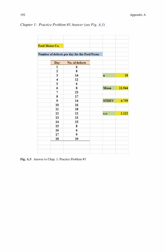
Chapter 1: Practice Problem #3 Answer (see Fig. A.3)
Fig. A.3 Answer to Chap. 1: Practice Problem #3
192 Appendix A

Chapter 2: Practice Problem #1 Answer (see Fig. A.4)
Fig. A.4 Answer to Chap. 2: Practice Problem #1
Appendix A 193

Chapter 2: Practice Problem #2 Answer (see Fig. A.5)
Fig. A.5 Answer to Chap. 2: Practice Problem #2
194 Appendix A

Chapter 2: Practice Problem #3 Answer (see Fig. A.6)
Fig. A.6 Answer to Chap. 2: Practice Problem #3
Appendix A 195

Chapter 3: Practice Problem #1 Answer (see Fig. A.7)
Fig. A.7 Answer to Chap. 3: Practice Problem #1
196 Appendix A

Chapter 3: Practice Problem #2 Answer (see Fig. A.8)
Fig. A.8 Answer to Chap. 3: Practice Problem #2
Appendix A 197

Chapter 3: Practice Problem #3 Answer (see Fig. A.9)
Fig. A.9 Answer to Chap. 3: Practice Problem #3
198 Appendix A
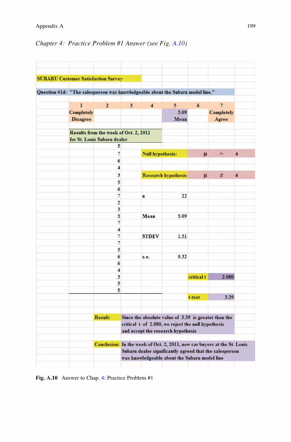
Chapter 4: Practice Problem #1 Answer (see Fig. A.10)
Fig. A.10 Answer to Chap. 4: Practice Problem #1
Appendix A 199

Chapter 4: Practice Problem #2 Answer (see Fig. A.11)
Fig. A.11 Answer to Chap. 4: Practice Problem #2
200 Appendix A

Chapter 4: Practice Problem #3 Answer (see Fig. A.12)
Fig. A.12 Answer to Chap. 4: Practice Problem #3
Appendix A 201

Chapter 5: Practice Problem #1 Answer (see Fig. A.13)
Fig. A.13 Answer to Chap. 5: Practice Problem #1
202 Appendix A
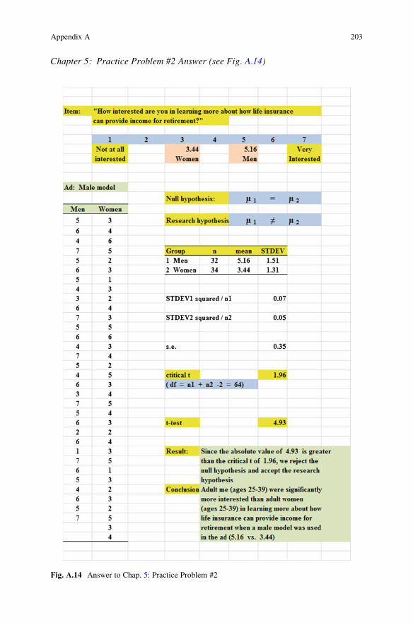
Chapter 5: Practice Problem #2 Answer (see Fig. A.14)
Fig. A.14 Answer to Chap. 5: Practice Problem #2
Appendix A 203

Chapter 5: Practice Problem #3 Answer (see Fig. A.15)
Fig. A.15 Answer to Chap. 5: Practice Problem #3
204 Appendix A
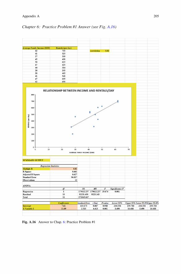
Chapter 6: Practice Problem #1 Answer (see Fig. A.16)
Fig. A.16 Answer to Chap. 6: Practice Problem #1
Appendix A 205

Chapter 6: Practice Problem #1 (continued)
1. a ¼ y-intercept ¼ 7:612. b ¼ slope ¼ 11:093. Y ¼ aþ bX
Y ¼ 7:61þ 11:09X4. Y ¼ 7:61þ 11:09ð50Þ
Y ¼ 7:61þ 554:5Y ¼ 562:11Y ¼ 562 rentals per day
206 Appendix A
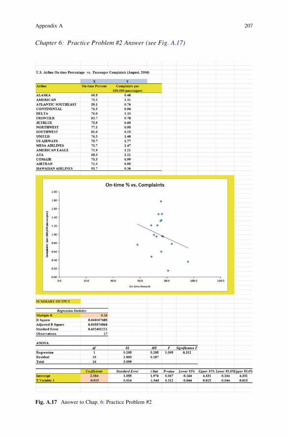
Chapter 6: Practice Problem #2 Answer (see Fig. A.17)
Fig. A.17 Answer to Chap. 6: Practice Problem #2
Appendix A 207

Chapter 6: Practice Problem #2 (continued)
1. a ¼ y - intercept ¼ 2:0842. b ¼ slope ¼ �0:015 ðnote the minus sign as the slope is negative)
3. Y ¼ aþ bXY ¼ 2:084� 0:015X
4. Y ¼ 2:084� 0:015ð80ÞY ¼ 2:084� 1:200Y ¼ 0:88 complaints per 100; 000 passengers
208 Appendix A

Chapter 6: Practice Problem #3 Answer (see Fig. A.18)
Fig. A.18 Answer to Chap. 6: Practice Problem #3
Appendix A 209
Chapter 6: Practice Problem #3 (continued)
1. r ¼ :952. a ¼ y - intercept ¼ �10:823. b ¼ slope ¼ 2:014. Y ¼ aþ bX
Y ¼ �10:82þ 2:01X5. Y ¼ �10:82þ 2:01ð25Þ
Y ¼ �10:82þ 50:25Y ¼ 39:43Y ¼ 39 copiers sold per month
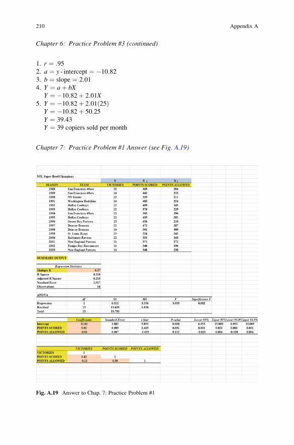
Chapter 7: Practice Problem #1 Answer (see Fig. A.19)
Fig. A.19 Answer to Chap. 7: Practice Problem #1
210 Appendix A

Chapter 7: Practice Problem #1 (continued)
1. Multiple correlation ¼ +.57
2. y-intercept ¼ 11.02
3. Points scored coefficient ¼ 0.01
4. Points allowed coefficient ¼ �0.01
5. Y ¼ aþ b1X1 þ b2X2
Y ¼ 11:02þ 0:01X1 � 0:01X2
6. Y ¼ 11:02þ 0:01ð526Þ � 0:01ð242ÞY ¼ 11:02þ 5:26� 2:42Y ¼ 13:86Y ¼ 14 wins (note that the Rams actually won 13 games in 1999 when they
won the Super Bowl)
7. 0.42
8. �0.12
9. 0.50
10. Points scored is a much better predictor of the number of wins because it has a
correlation of +.42 with the number of wins, and points allowed is only
correlated with the number of wins at �.12 (note that the plus or minus sign
is ignored when you try to decide which predictor is the better predictor of the
criterion; since .42 is greater than .12, points scored is the better predictor of
these two predictors)
11. The two predictors combined predict the number of wins at +.57, and this is
much better than the better single predictor’s correlation of +.42 with the
number of wins
Appendix A 211

Chapter 7: Practice Problem #2 Answer (see Fig. A.20)
Fig. A.20 Answer to Chap. 7: Practice Problem #2
Chapter 7: Practice Problem #2 (continued)
1. Multiple correlation ¼ þ:872. y - intercept ¼ �0:7393. HIGH SCHOOL GPA ¼ 0:3074. SAT VERBAL ¼ 0:0045. SAT MATH ¼ 0:0026. Y ¼ aþ b1X1 þ b2X2 þ b3X3
Y ¼ �0:739þ 0:307X1 þ 0:004X2 þ 0:002X3
7. Y ¼ �0:739þ 0:307ð3:15Þ þ 0:004ð490Þ þ 0:002ð480ÞY ¼ �0:739þ 0:97þ 1:96þ 0:96Y ¼ 3:15
8. +0.79
212 Appendix A
9. +0.83
10. +0.61
11. +0.81
12. +0.54
13. +0.54
14. SAT VERBAL is the best predictor of FROSH GPA because it has a correlation
of +.83 with FROSH GPA, and the other two predictors have a correlation that
is smaller than 0.83 (0.79 and 0.61)
15. The three predictors combined predict FROSH GPA at +.87, and this is only
slightly better than the best single predictor’s correlation of +.83 with FROSH
GPA
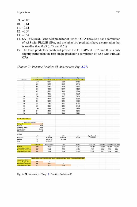
Chapter 7: Practice Problem #3 Answer (see Fig. A.21)
Fig. A.21 Answer to Chap. 7: Practice Problem #3
Appendix A 213

Chapter 7: Practice Problem #3 (continued)
1. Multiple correlation ¼ þ:912. y - intercept ¼ 60:073. Average Daily Traffic ¼ �0:024. Population ¼ 0:045. Average Income ¼ 0:056. Y ¼ aþ b1X1 þ b2X2 þ b3X3
Y ¼ 60:07� 0:02X1 þ 0:04X2 þ 0:05X3
7. Y ¼ 60:07� 0:02ð42; 000Þ þ 0:04ð23; 000Þ þ 0:05ð22; 000ÞY ¼ 60:07� 840þ 920þ 1100
Y ¼ 1240:07Y ¼ $1; 240; 000 or $1:24 million
8. +0.77
9. +0.42
10. +0.72
11. +0.53
12. �0.11
13. Average Daily Traffic is the best predictor of Annual Sales because it has a
correlation of +.77 with Annual Sales, and the other two predictors have a
correlation that is smaller than 0.77 (0.72 and 0.42)
14. The three predictors combined predict Annual Sales at +.91, and this is much
better than the best single predictor’s correlation of +.77 with Annual Sales
214 Appendix A

Chapter 8: Practice Problem #1 Answer (see Fig. A.22)
Fig. A.22 Answer to Chap. 8: Practice Problem #1
Appendix A 215

Chapter 8: Practice Problem #1 (continued)
1. Null hypothesis: mA ¼ mB ¼ mCResearch hypothesis: mA 6¼ mB 6¼ mC
2. MSb ¼ 41.50
3. MSw ¼ 3.24
4. F ¼ 12.81
5. Critical F ¼ 3.55
6. Since the F-value of 12.81 is greater than the critical F value of 3.55, we reject
the null hypothesis and accept the research hypothesis
7. There was a significant difference in the number of miles driven between the
three brands of tires
BRAND A vs. BRAND C
8. Null hypothesis: mA ¼ mCResearch hypothesis: mA 6¼ mC
9. 62
10. 66.33
11. Degrees of freedom ¼ 21 � 3 ¼ 18
12. Critical t ¼ 2.101
13. s.e. ANOVA ¼ SQRT(MSw � {1/5 + 1/6}) ¼ SQRT (3.24 � {0.20 + 0.167})
¼ SQRT(1.19) ¼ 1.09
14. ANOVA t ¼ (62 � 66.33) / 1.09 ¼ �3.97
15. Since the absolute value of �3.97 is greater than the critical t of 2.101, wereject the null hypothesis and accept the research hypothesis
16. Brand C was driven significantly more miles than Brand A (66,000 vs. 62,000)
BRAND A vs. BRAND B
17. Null hypothesis: mA ¼ mBResearch hypothesis: mA 6¼ mB
18. 62
19. 61.9
20. degrees of freedom ¼ 21 � 3 ¼ 18
21. critical t ¼ 2.101
22. s.e.ANOVA ¼ SQRT(MSw � {1/5 + 1/10}) ¼ SQRT(3.24 � {0.20 + 0.10})
¼ SQRT(0.972) ¼ 0.99
23. ANOVA t ¼ (62 � 61.9) / 0.99 ¼ 0.10
24. Since the absolute value of 0.10 is less than the critical t of 2.101, we accept thenull hypothesis
25. There was no difference in the number of miles driven between Brand A and
Brand B
216 Appendix A

BRAND B vs. BRAND C
26. Null hypothesis: mB ¼ mCResearch hypothesis: mB 6¼ mC
27. 61.90
28. 66.33
29. Degrees of freedom ¼ 21 � 3 ¼ 18
30. Critical t ¼ 2.101
31. s.e.ANOVA ¼ SQRT(MSw � {1/10 + 1/6}) ¼ SQRT(3.24 � {0.10 + 0.167})
¼ SQRT(0.87) ¼ 0.93
32. ANOVA t ¼ (61.90 � 66.33)/0.93 ¼ �4.76
33. Since the absolute value of �4.76 is greater than the critical t of 2.101, wereject the null hypothesis and accept the research hypothesis
34. Brand C was driven significantly more miles than Brand B (66,000 vs. 62,000)
SUMMARY
35. Brand C was driven significantly more miles than both Brand A and Brand B.
There was no difference in the number of miles driven between Brand A and
Brand B
36. Since our company’s Brand A was driven significantly less miles than Brand C,
we should never claim in our advertising for Brand A that we last more miles
than Brand C. Since our Brand A and Brand B were driven the same number of
miles, we should never claim that our tires last longer than Brand B
Appendix A 217

Chapter 8: Practice Problem #2 Answer (see Fig. A.23)
Fig. A.23 Answer to Chap. 8: Practice Problem #2
218 Appendix A

Chapter 8: Practice Problem #2 (continued)
1. Null hypothesis: m1 ¼ m2 ¼ m3 ¼ m4Research hypothesis: m1 6¼ m2 6¼ m3 6¼ m4
2. MSb ¼ 7057.47
3. MSw ¼ 90.12
4. F ¼ 78.31
5. critical F ¼ 2.82
6. Since the F-value of 78.31 is greater than the critical F value of 2.82, we reject
the null hypothesis and accept the research hypothesis
7. There was a significant difference in the number of Angus burgers sold in the
four types of advertising media
8. Null hypothesis: m3 ¼ m1Research hypothesis: m3 6¼ m1
9. 337.42
10. 299.58
11. Degrees of freedom ¼ 48 � 4 ¼ 44
12. Critical t ¼ 1.96
13. s.e.ANOVA ¼ SQRT(MSw � {1/12 + 1/12}) ¼ SQRT
(90.12 � {.083 + .083}) ¼ SQRT(14.96) ¼ 3.87
14. ANOVA t ¼ (337.42 � 299.58) / 3.87 ¼ 9.78
15. Since the absolute value of 9.78 is greater than the critical t of 1.96, we rejectthe null hypothesis and accept the research hypothesis
16. Billboard ads sold significantlymore Angus Burgers than Radio ads (337 vs. 300)
Appendix A 219

Chapter 8: Practice Problem #3 Answer (see Fig. A.24)
Fig. A.24 Answer to Chap. 8: Practice Problem #3
220 Appendix A

Chapter 8: Practice Problem #3 (continued)
1. Null hypothesis: mA ¼ mB ¼ mC ¼ mDResearch hypothesis: mA 6¼ mB 6¼ mC 6¼ mD
2. MSb ¼ 20.73
3. MSw ¼ 3.01
4. F ¼ 6.89
5. Critical F ¼ 2.77
6. Since the F-value of 6.89 is greater than the critical F value of 2.77, we reject
the null hypothesis and accept the research hypothesis
7. There was a significant difference in the believability of the four television
commercials
8. Null hypothesis: mB ¼ mDResearch hypothesis: mB 6¼ mD
9. 3.87
10. 5.87
11. Degrees of freedom ¼ 60 � 4 ¼ 56
12. Critical t ¼ 1.96
13. s.e.ANOVA ¼ SQRT(MSw � {1/15 + 1/15}) ¼ SQRT
(3.01 � {0.067 + 0.067}) ¼ SQRT(0.40) ¼ 0.64
14. ANOVA t ¼ (3.87 � 5.87) / 0.64 ¼ �3.125
15. Since the absolute value of �3.125 is greater than the critical t of 1.96, wereject the null hypothesis and accept the research hypothesis
16. Commercial D was significantly more believable than Commercial B (5.87
vs. 3.87)
Appendix A 221

Appendix B
Practice Test
Chapter 1: Practice Test
Suppose that you have been asked by the manager of the Webster Groves
Subaru dealer in St. Louis to analyze the data from a recent survey of its customers.
Subaru of America mails a “SERVICE EXPERIENCE SURVEY” to customers
who have recently used the Service Department for their car. Let’s try your Excel
skills on Item #10e of this survey (see Fig. A.25).
223

Fig. A.25 Worksheet data for Chap. 1 practice test (practical example)
(a) Create an Excel table for these data, and then use Excel to the right of the table
to find the sample size, mean, standard deviation, and standard error of the mean
for these data. Label your answers, and round off the mean, standard deviation,
and standard error of the mean to two decimal places.
(b) Save the file as: SUBARU8
224 Appendix B

Chapter 2: Practice Test
Suppose that you wanted to do a personal interview with a random sample of 12 of
your company’s 42 salespeople as part of a “company morale survey.”
(a) Set up a spreadsheet of frame numbers for these salespeople with the heading:
FRAME NUMBERS
(b) Then, create a separate column to the right of these frame numbers which
duplicates these frame numbers with the title: Duplicate frame numbers.
(c) Then, create a separate column to the right of these duplicate frame numbers
called RAND NO. and use the ¼RAND() function to assign random numbers to
all of the frame numbers in the duplicate frame numbers column, and change
this column format so that 3 decimal places appear for each random number.
(d) Sort the duplicate frame numbers and random numbers into a random order.
(e) Print the result so that the spreadsheet fits on one page.
(f) Circle on your printout the ID number of the first 12 salespeople that you would
interview in your company morale survey.
(g) Save the file as: RAND15
Important note: Note that everyone who does this problem will generate a differentrandom order of salesperson ID numbers since Excel assigns a different randomnumber each time the RAND() command is used. For this reason, the answer to thisproblem given in this Excel Guide will have a completely different sequence ofrandom numbers from the random sequence that you generate. This is normal andwhat is to be expected.
Chapter 3: Practice Test
Suppose that you have been asked to analyze the data from a flight on Southwest
Airlines from St. Louis to Boston in 2010. Southwest sent an online customer
satisfaction survey to a sample of its frequent fliers the day after the flight and asked
them to rate their flight on a 10-point scale with 1 ¼ extremely dissatisfied, and
10 ¼ extremely satisfied. The data for Item #2c appear in Fig. A.26.
Appendix B 225

Fig. A.26 Worksheet data for Chap. 3 practice test (practical example)
226 Appendix B

(a) Create an Excel table for these data, and use Excel to the right of the table to
find the sample size, mean, standard deviation, and standard error of the mean
for these data. Label your answers, and round off the mean, standard deviation,
and standard error of the mean to two decimal places in number format.
(b) By hand, write the null hypothesis and the research hypothesis on your printout.
(c) Use Excel’s TINV function to find the 95% confidence interval about the mean
for these data. Label your answers. Use two decimal places for the confidence
interval figures in number format.
(d) On your printout, draw a diagram of this 95% confidence interval by hand,
including the reference value.
(e) On your spreadsheet, enter the result.(f) On your spreadsheet, enter the conclusion in plain English.(g) Print the data and the results so that your spreadsheet fits on one page.
(h) Save the file as: south3
Chapter 4: Practice Test
Suppose that you have been asked by the American Marketing Association to
analyze the data from the 2010 Summer Educators’ conference in Boston. In
order to check your Excel formulas, you have decided to analyze the data for one
of these questions before you analyze the data for the entire survey, one item at a
time. The conference used a five-point scale with 1 ¼ Definitely Would Not, and
5 ¼ Definitely Would. A random sample of the hypothetical data for this one item
is given in Fig. A.27.
Appendix B 227

Fig. A.27 Worksheet data for Chap. 4 practice test (practical example)
228 Appendix B

(a) Write the null hypothesis and the research hypothesis on your spreadsheet.
(b) Create a spreadsheet for these data, and then use Excel to find the sample size,
mean, standard deviation, and standard error of the mean to the right of the data
set. Use number format (3 decimal places) for the mean, standard deviation, and
standard error of the mean.
(c) Type the critical t from the t-table in Appendix E onto your spreadsheet, and
label it.
(d) Use Excel to compute the t-test value for these data (use 3 decimal places) and
label it on your spreadsheet.
(e) Type the result on your spreadsheet, and then type the conclusion in plainEnglish on your spreadsheet.
(f) Save the file as: BOS2
Chapter 5: Practice Test
Massachusetts Mutual Financial Group (2010) placed a full-page color ad in TheWall Street Journal in which it used a male model hugging a 2-year old daughter.
The ad had the headline and subheadline:
WHAT IS THE SIGN OF A GOOD DECISION?
It’s knowing your life insurance can help provide income for retirement. And peaceof mind until you get there.
Since the majority of the subscribers to The Wall Street Journal are men, an
interesting research question would be the following:
Research question: “Does the gender of the model affect adult men’s willingness
to learn more about how life insurance can provide income
for retirement?”
Suppose that you have shown two groups of adult males (ages 25–44) a mockup
of an ad such that one group of males saw the ad with a male model, while the other
group of males saw the same ad with a female model. (You randomly assigned
these males to one of the two experimental groups.) The two groups were kept
separate during the experiment and could not interact with one another.
At the end of a 1-hour discussion of the mockup ad, the respondents were asked
the question given in Fig. A.28.
Fig. A.28 Survey item for a mockup ad (practical example)
Appendix B 229

The resulting data for this one item appear in Fig. A.29.
Fig. A.29 Worksheet data for Chap. 5 practice test (practical example)
230 Appendix B

(a) Write the null hypothesis and the research hypothesis.
(b) Create an Excel table that summarizes these data.
(c) Use Excel to find the standard error of the difference of the means.
(d) Use Excel to perform a two-group t-test. What is the value of t that you obtain
(use two decimal places)?
(e) On your spreadsheet, type the critical value of t using the t-table in Appendix E.(f) Type the result of the test on your spreadsheet.
(g) Type your conclusion in plain English on your spreadsheet.
(h) Save the file as: lifeinsur3
(i) Print the final spreadsheet so that it fits on one page.
Chapter 6: Practice Test
Is there a relationship between on-time performance and the number of passenger
complaints for US major airlines? An article from The Wall Street Journal(McCartney 2010) presented the data given in Fig. A.30.
Fig. A.30 Worksheet data for Chap. 6 practice test (practical example)
Create an Excel spreadsheet and enter the data using on-time arrivals as the
independent variable (predictor) and the number of passenger complaints per
million passengers as the dependent variable (criterion).
(a) Use Excel’s ¼correl function to find the correlation between these two sets of
scores, and round off the result to two decimal places.
(b) Create an XY scatterplot of these two sets of data below the table such that:
• Top title: RELATIONSHIP BETWEEN ON-TIME % AND PASSENGER
COMPLAINTS
• x-axis title: % On-time Arrivals
• y-axis title: Passenger Complaints per million passengers
• Move the chart below the table.
• Resize the chart so that it is 7 columns wide and 25 rows long.
Appendix B 231

• Delete the legend.
• Delete the gridlines.
(c) Create the least squares regression line for these data on the scatterplot.
(d) Use Excel to run the regression statistics to find the equation for the least-squares regression line for these data and display the results below the chart on
your spreadsheet. Use number format (2 decimal places) for the correlation and
for the coefficients.
Print just the input data and the chart so that this information fits on one page.
Then, print just the regression output table on a separate page so that it fits on
that separate page in portrait format.
By hand:
(a) Circle and label the value of the y-intercept and the slope of the regression lineonto that separate page.
(b) Write the regression equation by hand on your printout for these data (use two
decimal places for the y-intercept and the slope).
(c) Circle and label the correlation between these two sets of scores in the
regression analysis summary output table on your printout.
(d) Underneath the regression equation you wrote by hand on your printout, use the
regression equation to predict the number of passenger complaints you would
expect for an on-time arrival of 80%.(e) Read from the graph the number of passenger complaints you would predict for
an on-time arrival rate of 76% and write your answer in the space immediately
below:
(f) Save the file as: ontime3
Chapter 7: Practice Test
The National Football League (2009) and ESPN (2009a, 2009b) record a large
number of statistics about players, teams, and leagues on their Web sites. Suppose
that you wanted to record the data for 2009 and create a multiple regression
equation for predicting the number of wins during the regular season based on
four predictors: (1) yards gained on offense, (2) points scored on offense, (3) yards
allowed on defense, and (4) points allowed on defense. These data are given in
Fig. A.31.
232 Appendix B

Fig. A.31 Worksheet data for Chap. 7 practice test (practical example)
(a) Create an Excel spreadsheet using Games Won as the criterion (Y), and the
other variables as the four predictors of this criterion.
(b) Use Excel’s multiple regression function to find the relationship between these
variables and place it below the table.
(c) Use number format (2 decimal places) for the multiple correlation on the
Summary Output, and use number format (three decimal places) for the
coefficients in the Summary Output
(d) Print the table and regression results below the table so that they fit on one page.
Appendix B 233
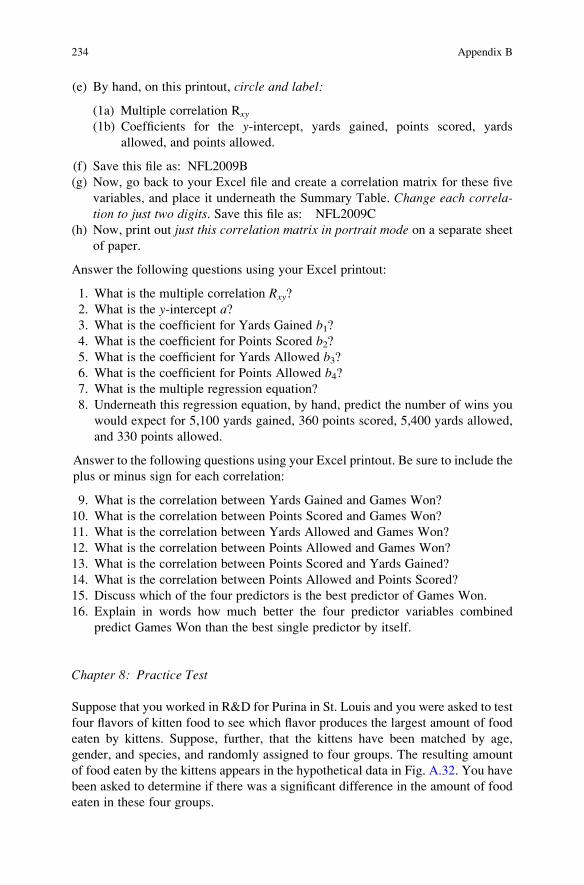
(e) By hand, on this printout, circle and label:
(1a) Multiple correlation Rxy
(1b) Coefficients for the y-intercept, yards gained, points scored, yards
allowed, and points allowed.
(f) Save this file as: NFL2009B
(g) Now, go back to your Excel file and create a correlation matrix for these five
variables, and place it underneath the Summary Table. Change each correla-tion to just two digits. Save this file as: NFL2009C
(h) Now, print out just this correlation matrix in portrait mode on a separate sheet
of paper.
Answer the following questions using your Excel printout:
1. What is the multiple correlation Rxy?
2. What is the y-intercept a?3. What is the coefficient for Yards Gained b1?4. What is the coefficient for Points Scored b2?5. What is the coefficient for Yards Allowed b3?6. What is the coefficient for Points Allowed b4?7. What is the multiple regression equation?
8. Underneath this regression equation, by hand, predict the number of wins you
would expect for 5,100 yards gained, 360 points scored, 5,400 yards allowed,
and 330 points allowed.
Answer to the following questions using your Excel printout. Be sure to include the
plus or minus sign for each correlation:
9. What is the correlation between Yards Gained and Games Won?
10. What is the correlation between Points Scored and Games Won?
11. What is the correlation between Yards Allowed and Games Won?
12. What is the correlation between Points Allowed and Games Won?
13. What is the correlation between Points Scored and Yards Gained?
14. What is the correlation between Points Allowed and Points Scored?
15. Discuss which of the four predictors is the best predictor of Games Won.
16. Explain in words how much better the four predictor variables combined
predict Games Won than the best single predictor by itself.
Chapter 8: Practice Test
Suppose that you worked in R&D for Purina in St. Louis and you were asked to test
four flavors of kitten food to see which flavor produces the largest amount of food
eaten by kittens. Suppose, further, that the kittens have been matched by age,
gender, and species, and randomly assigned to four groups. The resulting amount
of food eaten by the kittens appears in the hypothetical data in Fig. A.32. You have
been asked to determine if there was a significant difference in the amount of food
eaten in these four groups.
234 Appendix B

Fig. A.32 Worksheet data for Chap. 8 practice test (practical example)
(a) Enter these data on an Excel spreadsheet.
(b) On your spreadsheet, write the null hypothesis and the research hypothesis for
these data
(c) Perform a one-way ANOVA test on these data, and show the resulting ANOVA
table underneath the input data for the four types of kitten food.
(d) If the F-value in the ANOVA table is significant, create an Excel formula to
compute the ANOVA t-test comparing the amount of food eaten in Group B
against the amount of food eaten in Group D, and show the results below the
ANOVA table on the spreadsheet (put the standard error and the ANOVA t-testvalue on separate lines of your spreadsheet; use two decimal places for each
value)
(e) Print out the resulting spreadsheet so that all of the information fits on one page
(f) On your printout, label by hand the MS between groups and the MS within
groups.
(g) Circle and label the value for F on your printout for the ANOVA of the input
data.
(h) Label by hand on the printout the mean for Group B and the mean for Group D
that were produced by your ANOVA formulas.
Save the spreadsheet as: kitten2
On a separate sheet of paper, now do the following by hand:
(i) Find the critical value of F using the ANOVA Single Factor table that you
created.
(j) Write a summary of the results of the ANOVA test for the input data.
(k) Write a summary of the conclusion of the ANOVA test in plain English for the
input data.
Appendix B 235

(l) Write the null hypothesis and the research hypothesis comparing Group B
versus Group D.
(m) Compute the degrees of freedom for the ANOVA t-test by hand for four flavors.(n) Write the critical value of t for the ANOVA t-test using the table in
Appendix E.
(o) Write a summary of the result of the ANOVA t-test.(p) Write a summary of the conclusion of the ANOVA t-test in plain English.
References
ESPN. NFL Team Total Offense Statistics – 2009. Retrieved December 9, 2010, from http://espn.
go.com/nfl/statistics/team/_/stat/total/year/2009
ESPN. NFL Team Total Defense Statistics – 2009. Retrieved December 9, 2010, from http://espn.
go.com/nfl/statistics/team/_/stat/total/position/defense/year/2009
Mass Mutual Financial Group. What is the Sign of a Good Decision? (Advertisement) The WallStreet Journal, September 29, 2010, p. A22.
McCartney, S. An airline report card: fewer delays, hassles last year, but bumpy times may be
ahead. The Wall Street Journal (2010 January 7), pp. D1, D3.
National Football League. Standings [2009 Regular Season by league]. Retrieved December 9, 2010
from http://www.nfl.com/standings?category¼league&season¼2009-REG&split¼Overall
236 References

Appendix C
Answers to Practice Test
Practice Test Answer: Chapter 1 (see Fig. A.33)
Fig. A.33 Practice test answer to Chap. 1 problem
237

Practice Test Answer: Chapter 2 (see Fig. A.34)
Fig. A.34 Practice test answer to Chap. 2 problem
238 Appendix C

Practice Test Answer: Chapter 3 (see Fig. A.35)
Fig. A.35 Practice test answer to Chap. 3 problem
Appendix C 239

Practice Test Answer: Chapter 4 (see Fig. A.36)
Fig. A.36 Practice test answer to Chap. 4 problem
240 Appendix C

Practice Test Answer: Chapter 5 (see Fig. A.37)
Fig. A.37 Practice test answer to Chap. 5 problem
Appendix C 241

Practice Test Answer: Chapter 6 (see Fig. A.38)
Fig. A.38 Practice test answer to Chap. 6 problem
Practice Test Answer: Chapter 6: (continued)
(a) a ¼ y - intercept ¼ 64:49b ¼ slope ¼ �0:69 (note the minus sign as the slope is negative)
(b) Y ¼ aþ bXY ¼ 64:49� 0:69X
(c) r ¼ correlation ¼ �0:41 (note that the correlation is negative because the
slope is negative!)
(d) Y ¼ 64:49� 0:69ð80ÞY ¼ 64:49� 55:20Y ¼ 9.29 complaints per million passengers
(e) About 12 complaints per million passengers
242 Appendix C

Practice Test Answer: Chapter 7 (see Fig. A.39)
Fig. A.39 Practice test answer to Chap. 7 problem
Appendix C 243

Practice Test Answer: Chapter 7 (continued)
1. Rxy ¼ +0.94
2. y-Intercept ¼ 0.601
3. Yards Gained ¼ 0.000
4. Points Scored ¼ 0.030
5. Yards Allowed ¼ 0.001
6. Points Allowed ¼ �0.026
7. Y ¼ aþ b1X1 þ b2X2 þ b3X3 þ b4X4
Y ¼ 0:601þ 0:000X1 þ 0:030X2 þ 0:001X3 � 0:026X4
8. Y ¼ 0:601þ 0:000ð5100Þ þ 0:030ð360Þ þ 0:001ð5400Þ � 0:026ð330ÞY ¼ 0:601þ 0:0þ 10:8þ 5:4� 8:58Y ¼ 8.22
Y ¼ 8 Games Won
9. +0.77
10. +0.88
11. �0.56
12. �0.68
13. +0.87
14. �0.46
15. The best predictor of GamesWon was Points Scored with a correlation of +0.88
16. The four predictors combined predict Games Won with a correlation of +0.94
which is much better than the best single predictor by itself
244 Appendix C

Practice Test Answer: Chapter 8 (see Fig. A.40)
Fig. A.40 Practice test answer to Chap. 8 problem
Practice Test Answer: Chapter 8 (continued)
(f) MSb ¼ 1143.18 and MSw ¼ 15.58
(g) F ¼ 73.40
(h) Mean Group B ¼ 23.10, and Mean Group D ¼ 38.50
(i) critical F ¼ 2.84
(j) Results: Since 73.40 is greater than the critical F of 2.84, we reject the null
hypothesis and accept the research hypothesis
Appendix C 245

(k) Conclusion: There was a significant difference in the amount of food eaten by
the kittens in the four flavors of kitten food
(l) Null hypothesis : mB ¼ mDResearch hypothesis : mB 6¼ mD
(m) df ¼ nTOTAL � k ¼ 44� 4 ¼ 40
(n) critical t ¼ 1:96(o) Result: Since the absolute value of �9.11 is greater than the critical t of 1.96,
we reject the null hypothesis and accept the research hypothesis
(p) Conclusion: The kittens ate significantly more of Flavor D than Flavor B
(38.50 vs. 23.10)
246 Appendix C

Appendix D
Statistical Formulas
Mean �X ¼P
X
nStandard Deviation
STDEV ¼ S ¼ffiffiffiffiffiffiffiffiffiffiffiffiffiffiffiffiffiffiffiffiffiffiffiffiP ðX � �XÞ2
n� 1
s
Standard error of the means.e: ¼ S �X ¼ S
ffiffiffin
pConfidence interval about the mean �X � t S �X
where S �X ¼ Sffiffiffin
pOne-group t-test
t ¼�X � mS �X
where S �X ¼ Sffiffiffin
p
Two-group t-test
(a) When both groups have a
sample size greater than 30 t ¼�X1 � �X2
S �X1� �X2
where S �X1� �X2¼
ffiffiffiffiffiffiffiffiffiffiffiffiffiffiffiffiffiffiffiS1
2
n1þ S2
2
n2
s
and where df ¼ n1 þ n2 � 2
(b) When one or both groups have
a sample size less than 30 t ¼�X1 � �X2
S �X1� �X2
where S �X1� �X2¼
ffiffiffiffiffiffiffiffiffiffiffiffiffiffiffiffiffiffiffiffiffiffiffiffiffiffiffiffiffiffiffiffiffiffiffiffiffiffiffiffiffiffiffiffiffiffiffiffiffiffiffiffiffiffiffiffiffiffiffiffiffiffiffiffiffiffiffiffiffiffiffiffiffiffiðn1 � 1ÞS12 þ ðn2 � 1ÞS22
n1 þ n2 � 2
1
n1þ 1
n2
� �s
and where df ¼ n1 þ n2 � 2
Correlationr ¼
1n�1
PðX � �XÞðY � �YÞSxSy
where Sx ¼ standard deviation of X
and where Sy ¼ standard deviation of Y
(continued)
247

(continued)
Simple linear regression Y ¼ aþ bX
where a ¼ y-intercept and b ¼ slope of the line
Multiple regression equation Y ¼ aþ b1X1 þ b2X2 þ b3X3 þ etc:
where a ¼ y-intercept
One-way ANOVA F-test F ¼ MSb=MSwANOVA t-test
ANOVA t ¼�X1 � �X2
s.e:ANOVA
where s.e:ANOVA ¼ffiffiffiffiffiffiffiffiffiffiffiffiffiffiffiffiffiffiffiffiffiffiffiffiffiffiffiffiffiffiffiffi
MSw1
n1þ 1
n2
� �s
and where df ¼ nTOTAL � k
where nTOTAL ¼ n1 þ n2 þ n3 þ etc:
and where k ¼ the number of groups
248 Appendix D

Appendix E
t-Table
249
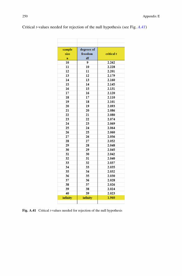
Critical t-values needed for rejection of the null hypothesis (see Fig. A.41)
Fig. A.41 Critical t-values needed for rejection of the null hypothesis
250 Appendix E

Index
A
Absolute value of number, 68–69
Analysis of variance
ANOVA t-test formula, 176
degrees of freedom, 177
Excel commands, 178–180
formula, 173–174
interpreting the summary table,
173–174
s.e. formula for ANOVA t-test, 176ANOVA. See Analysis of varianceANOVA t-test. See Analysis of varianceAverage function. See Mean
C
Centering information within cells, 7
Chart
adding the regression equation,
140–142
changing the width and height, 5–6
creating a chart, 120–129
drawing the regression line onto the
chart, 120–129
moving the chart, 125, 126
printing the spreadsheet, 130–131
reducing the scale, 130
scatter chart, 122
titles, 122–125
Column width (changing), 5–6, 155
Confidence interval about the mean
95% confident, 37–47, 76
drawing a picture, 45
formula, 41
lower limit, 38–43, 45–47, 53,
63, 65
upper limit, 38–43, 45–47, 53, 63, 65
Correlation
formula, 114
negative correlation, 109, 111, 112,
138, 142–143, 149
positive correlation, 109–111, 115,
120, 143, 149, 163
9 steps for computing r, 114–116CORREL function. See CorrelationCOUNT function, 9–10, 53
Critical t-value, 41, 59, 68–71, 74, 79,84–86, 90, 91, 106, 177, 178
D
Data Analysis ToolPak, 132–134, 169
Data/Sort commands, 27
Degrees of freedom, 85, 87, 88, 90,
99, 177
F
Fill/Series/Columns commands, 4–5
step value/stop value commands,
5, 22
Formatting numbers
currency format, 15–16
decimal format, 136
H
Home/Fill/Series commands, 4
Hypothesis testing
decision rule, 53, 68–69
null hypothesis, 49–62, 64, 68, 71,
72, 75, 77, 79, 83–84, 86–91,
93, 95–98, 102, 104–106,
174–176, 178
251

Hypothesis testing (cont.)rating scale hypotheses, 51
research hypothesis, 49–59, 61, 62, 64, 68,
71, 72, 75, 77, 79, 83–84, 86–91, 93,
95–98, 102, 104–106, 174–176, 178
stating the conclusion, 54, 55, 57, 58
stating the result, 58, 59
7 steps for hypothesis testing, 52–58, 67–71
M
Mean, 1–20, 37–65, 67–106, 113–119, 169,
173–176, 178, 180
formula, 2
Multiple correlation
correlation matrix, 160–163
excel commands, 178–180
Multiple regression
correlation matrix, 160–163
equation, 153
Excel commands, 178–180
predicting Y, 153
N
Naming a range of cells, 8–9
Null hypothesis. See Hypothesis testing
O
One-group t-test for the mean
absolute value of a number, 68–69
formula, 67
hypothesis testing, 67–71
s.e. formula, 67
7 steps for hypothesis testing, 67–71
P
Page Layout/Scale to Fit commands, 31
Population mean, 37–39, 49, 50, 67, 69,
83, 90, 91, 169, 174–176, 178
Printing a spreadsheet
entire worksheet, 144–145
part of the worksheet, 144–145
printing a worksheet to fit onto one page,
31–34, 130–131
R
RAND(). See Random number generator
Random number generator
duplicate framenumbers, 23, 24, 26–29, 35, 36
frame numbers, 21–30, 35, 36
sorting duplicate frame numbers, 27–30,
35, 36
Regression, 109–151, 153–168
Regression equation
adding it to the chart, 140–143
formula, 139
negative correlation, 109, 111, 112, 138,
142–143, 149
predicting Y from x, 109, 120, 121, 132,
139–140, 155
slope, b, 138writing the regression equation using the
Summary Output, 159
y-intercept, a, 138–141Regression line, 120–131, 138–143, 147–150
Research hypothesis. See Hypothesis testing
S
Sample size, 1–20, 38, 41–43, 45, 46, 48,
53, 60, 62, 64, 67, 70, 72, 73, 77, 79,
81–85, 87, 90–93, 97, 99, 105, 113,
114, 118, 119, 172, 176, 177
COUNT function, 9–10, 53
Saving a spreadsheet, 13–14
Scale to Fit commands, 31, 46
s.e. See Standard error of the mean
Standard deviation, 1–20, 38, 39, 43,
46, 53, 60, 62, 64, 67, 69, 72,
77, 79, 81–83, 87, 88, 91–93, 97,
104–106, 118
formula, 2
Standard error of the mean, 1–20, 38–40,
42, 43, 46, 53, 60, 62, 64, 67, 69,
74, 77, 79, 90, 91
formula, 3
STDEV. See Standard deviation
T
t-table, 249–250Two-group t-test
basic table, 83
degrees of freedom, 85, 87, 88, 90,
99, 177
drawing a picture of the means, 89
formula, 99
formula #1, 90
formula #2, 99
hypothesis testing, 82–90
s.e. formula, 90, 99
9 steps in hypothesis testing, 82–90
252 Index