i
Anthropogenic Emissions ofGreenhouse Gases and Natural Causes
of Climate Change
Kontotasiou VasilikiSID: 3302130018
SCHOOL OF SCIENCE & TECHNOLOGYA thesis submitted for the degree of
Master of Science (MSc) in Energy Systems
NOVEMBER 2015THESSALONIKI – GREECE

ii
Anthropogenic Emissions ofGreenhouse Gases and Natural Causes
of Climate Change
Kontotasiou VasilikiSID: 3302130018
Supervisor: Dr. Theologos Dergiades
Invalid signature
XTheologos DergiadesDrSigned by: Theologos Dergiades
Supervising Committee Members: Dr. Georgios Martinopoulos
Dr. Panagiotidis
iii
AbstractThis dissertation was written as a part of the MSc in Energy Systems at the International
Hellenic University. Climate change is a growing problem, studied extensively during the
past few decades, focusing especially on our tampering with the environment. This
dissertation attempts to augment the work of Stern and Kaufmann (2014) through
several variables’ effects on temperature, with the implementation of more recent
econometric techniques. Additionally, it concentrates on possible explanations behind
dissimilar, with the aforementioned study, results, as well as on the outcomes’
progression over time. The analysis includes stationarity, cointegration and causality
investigation, achieved with more than two tests in each case, between several gases
radiative forcings and both HADCRUT4 and GISSv3 temperature time series, through a
direct, in both completely and partially aggregated models, as well as through an indirect
approach, in an entirely disaggregated model. Four scenarios are tested, and samples lie
within the 1850 to 2011 and 1958 to 2011 time span. The investigation of the evolution
of all the aforementioned causal relationships in all models and scenarios with time, using
the fixed window on a rolling basis method, is considered a novelty as regards the climate
change research. Results suggest that total, natural, anthropogenic and Greenhouse
Gases’ radiative forcings cause temperature to change, while human induced sulfur
emissions, solar irradiance and black carbon do not, throughout the largest part of the
time period. Most of this research outcome is consistent with theory and Stern and
Kaufmann (2014), with possible minor declination reasons the slightly different approach
to Toda Yamamoto causality testing.

iv
Acknowledgements
Although the cover of this dissertation bears only my own name, I could have never had
accomplished it without the dedicated work and support of many others, to whom I use
this paragraph to communicate my sincerest gratitude. I would like to express the deepest
appreciation to my supervising Professor Dr. Theologos Dergiades, for his many hours
spend teaching and guiding me throughout the whole experience, answering all my
inquiries, always supporting and encouraging my every step. I would also like to
acknowledge a special debt to my family, my fiancé Alexis and his family, for their
expression of love and support in every way possible during this journey.
Kontotasiou Vasiliki
11/12/2015

v
Table of ContentsABSTRACT....................................................................................................................................................................................III
ACKNOWLEDGEMENTS ...................................................................................................................................................... IV
LIST OF TABLES ....................................................................................................................................................................... VI
LIST OF FIGURES................................................................................................................................................................... VII
1. INTRODUCTION................................................................................................................................................................ 1
2. LITERATURE REVIEW....................................................................................................................................................32.1. DETECTION AND ATTRIBUTION METHODS.............................................................................................................4
2.1.1. Non – Optimal Approach .................................................................................................................................42.1.2. Optimal Approach .............................................................................................................................................5
2.1.2.1. Optimal Filtering Approach ............................................................................................................................ 5
2.1.2.2. Optimal Fingerprint Approach........................................................................................................................ 5
2.1.2.3. Multiple Linear Regression Analysis............................................................................................................... 9
2.1.2.4. Multivariate Linear Regression Analysis ....................................................................................................... 12
2.1.3. Cointegration Analysis .................................................................................................................................... 142.1.3.1. Ordinary Least Squares (OLS) approach. ..................................................................................................... 14
2.1.3.2. Johansen approach. ....................................................................................................................................... 18
2.1.3.3. Polynomial Cointegration ............................................................................................................................. 23
2.2. LITERATURE REVIEW CONCLUSIONS ......................................................................................................................252.3. LITERATURE REVIEW SUMMARY ...............................................................................................................................29
3. METHODOLOGICAL FRAMEWORK ......................................................................................................................323.1. STATIONARITY TESTS....................................................................................................................................................32
3.1.1. Dickey – Fuller Unit Root Test...................................................................................................................... 333.1.2. Augmented Dickey – Fuller Unit Root Test ................................................................................................ 343.1.3. ADF – GLS Unit Root Test ............................................................................................................................ 353.1.4. Phillips – Perron Unit Root Test ................................................................................................................... 353.1.5. KPSS Stationarity Test .................................................................................................................................... 36
3.2. COINTEGRATION ANALYSIS ........................................................................................................................................373.2.1. Engle and Granger Cointegration Test ........................................................................................................ 373.2.2. Johansen Cointegration Test.......................................................................................................................... 38
3.3. CAUSALITY TESTS ...........................................................................................................................................................413.3.1. Granger Causality Test.................................................................................................................................... 413.3.2. Toda Yamamoto Causality Test .................................................................................................................... 42
4. DATA SOURCES.................................................................................................................................................................444.1. TEMPERATURE ................................................................................................................................................................44
4.1.1. HADCRUT4 ..................................................................................................................................................... 444.1.2. GISSv3 ............................................................................................................................................................... 444.1.3. Ocean Heat Content........................................................................................................................................ 45
4.2. RADIATIVE FORCING .....................................................................................................................................................454.2.1. Carbon Dioxide, Methane, Nitrous Oxide and CFCs ................................................................................ 454.2.2. Volcanic Sulfate Aerosols ................................................................................................................................ 464.2.3. Anthropogenic Sulfur Emissions ................................................................................................................... 47

vi
4.2.4. Solar Irradiance, Black and Organic Carbon ............................................................................................... 48
5. EMPIRICAL APPLICATION.........................................................................................................................................495.1. STATIONARITY TEST RESULTS ...................................................................................................................................515.2. COINTEGRATION ANALYSIS ........................................................................................................................................52
5.2.1. Engle – Granger Cointegration Test Results ............................................................................................... 525.2.2. Johansen Cointegration Test Results............................................................................................................ 54
5.3. CAUSALITY TEST RESULTS...........................................................................................................................................555.3.1. Granger Causality Test Results...................................................................................................................... 555.3.3. Rolling Window Results.................................................................................................................................. 64
6. DISCUSSION........................................................................................................................................................................70
7. CONCLUSIONS..................................................................................................................................................................76
REFERENCES .............................................................................................................................................................................78
APPENDICES ...............................................................................................................................................................................88A. TEMPERATURE TIME SERIES DATA CONSTRUCTION AND THE RELATED UNCERTAINTIES .............................88B. COMPLETELY DISAGGREGATED MODEL CAUSALITY INVESTIGATION ...............................................................89C. WHAT CHANGES IF THERE IS COINTEGRATION IN MODEL III AND SCENARIO 4 OF MODEL II?........................94D. ADDITIONAL FIGURES .................................................................................................................................................95

vii
List of Tables
Table 1 Literature Review Summary Table ......................................................................................................................... 29Table 2 Stationarity Test Results ............................................................................................................................................ 50Table 3 Order of Integration of each variable as indicated by the majority of the stationarity tests ............... 51Table 4 Engle and Granger Cointegration Test Results ................................................................................................. 52Table 5 Johansen Cointegration Test Results .................................................................................................................... 53Table 6 Johansen Cointegration Test Optimal Lag Lengths......................................................................................... 54Table 7 Granger Causality Test Lag Lengths ..................................................................................................................... 55Table 8 Granger Causality Test Results (HADCRUT4)................................................................................................. 56Table 9 Granger Causality Test Results (GISSv3) ............................................................................................................ 57Table 10 Toda Yamamoto Causality Test VAR Lag Lengths ....................................................................................... 60Table 11 Toda Yamamoto Causality Test Results (HADCRUT4) .............................................................................. 61Table 12 Toda Yamamoto Causality Test Results (GISSv3) ......................................................................................... 62Table 13 Toda Yamamoto Causality VAR Lag Lengths (Rolling)............................................................................... 64Table 14 Order of Integration of GHGs as indicated by the majority of the stationarity tests ......................... 83Table 15 Granger Causality Test Results of Model III with Disaggregated GHGs (VAR) ................................ 84Table 16 Granger Causality Test Optimal Lag Lengths (VECM)................................................................................ 85Table 17 Granger Causality Test Results of Model III with Disaggregated GHGs (VECM) ............................ 85Table 18 Toda Yamamoto Causality Test Results of Model III with Disaggregated GHGs.............................. 86Table 19 Granger Causality Test Results – VECM.................................................................................................88
List of FiguresFigure 1 HADCRUT4, GISSv3 and Ocean Heat Content....................................................................................44Figure 2 Radiative Forcings of CO2, CH4, N2O, CFC11 and CFC12..................................................................45Figure 3 Radiative Forcing of Volcanic Sulfate Aerosols ......................................................................................45Figure 4 Radiative Forcing of Anthropogenic Sulfur Emissions .........................................................................46Figure 5 Radiative Forcing of Solar Irradiance .......................................................................................................46Figure 6 Radiative Forcing of Black and Organic Carbon ....................................................................................46Figure 7 Radiative Forcing of Greenhouse Gases ..................................................................................................47Figure 8 ........................................................................................................................................................................48Figure 9 Toda Yamamoto Results (Rolling) ............................................................................................................63Figure 10 Toda Yamamoto Results (Rolling) ..........................................................................................................64Figure 11 Toda Yamamoto Results (Rolling)...........................................................................................................65Figure 12 Toda Yamamoto Results (Rolling) ..........................................................................................................66Figure 13 Toda Yamamoto Results (Rolling)...........................................................................................................87Figure 14 Toda Yamamoto Results (Rolling) .........................................................................................................88

1
CHAPTER 11. Introduction
Understanding in which manner our planet works is of outmost importance for our survival.
We have reached a point where it is more than obvious that climate has been altered. Related
research is only necessary in order to discover the reasons behind it, and subsequently to
decide how we can stop it, or at least moderate its effects. The majority of the related studies
agree that increase in observed global temperature records is caused by natural phenomena,
climate feedbacks and several gases’ concentration accretions. Human related emissions
appear to be substantially higher today compared to their pre-industrial levels, placing the
anthropogenic climate change theory under investigation.
Such observations led to research such as Stern and Kaufmann (2014), testing for
causality between several emissions’ radiative forcings and temperature, while investigating
the human-related and natural reasons behind climate change. Stern and Kaufmann (2014)
developed three Models, through which they explored possible causal relationships between
two temperature time series (HADCRUT4 and GISSv3) and several gases, during the 1850 to
2011 and 1958 to 2011 time periods. Total (Natural and Anthropogenic) radiative forcing is
used in the first Model, and it is disaggregated into Natural (volcanic sulfate aerosols and
solar irradiance) and Anthropogenic (anthropogenic sulfur emissions, greenhouse gases and
black carbon) radiative forcings in the second Model. In the third Model all radiative forcings
of the investigated time series are disaggregated, and the possible causal relationships with
temperature are explored. Four scenarios are developed, regarding uncertainties in the relative
size of black carbon and anthropogenic sulfur emissions. Stern and Kaufmann (2014) find
that total and natural radiative forcings causes both temperature time series, while
anthropogenic radiative forcings cause temperature only in the fourth scenario. It is
inconclusive if temperature causes anthropogenic forcing, while a two–way causal
relationship is found to exist between temperature and carbon dioxide. Furthermore, Stern
and Kaufmann (2014) find that greenhouse gases and anthropogenic sulfate aerosol cause
temperature in all scenarios, while there is no causal effect between black carbon and
temperature, volcanic aerosols play a big role and solar irradiance much less. Their overall
conclusion was that human induced emissions partly cause global temperature increase.
The purpose of this dissertation is to augment the work of Stern and Kaufmann
(2014) through more detailed investigation of their data set. The following questions are
addressed. Do natural, anthropogenic and individual radiative forcings’ fluctuations cause
temperature to change? Is the answer to this initial question similar to the outcome of Stern

2
and Kaufmann (2014) research, and if it differs, why would this occur? Are the results of the
first question robust throughout the time period under review, and if this proves to be
otherwise, why? These questions are addressed using the same Models and scenarios during
the same time period. Subsequently, the robustness of the results is examined through
testing for causality through a fixed window on a rolling basis method.
The findings agree with Stern and Kaufmann (2014) research, regarding natural,
anthropogenic and total radiative forcings causing temperature change. These results are
considerably robust throughout the sample period. This also applies to the result of
greenhouse gases’ radiative forcing causing temperature, which is highly robust as well,
whereas it is inconclusive if the same applies for the volcanic sulfate aerosols one, that is also
similar to the Stern and Kaufman (2014) result. The anthropogenic sulfate aerosols radiative
forcing causing temperature change result, contrary to the aforementioned study’s outcome,
is negative and this is robust only for the Met Office Hadley Centre Observations Dataset
(HADCRUT4). With regard to solar irradiance not causing temperature change, results
agree, and are robust across all specifications, while the aggregated influence of it with
volcanic sulfate aerosols on temperature disagrees with the Stern and Kaufmann (2014)
result, and it is robust merely for the Goddard Institute for Space Studies dataset (GISSv3).
It is strongly indicated that temperature change causes greenhouse gas concentrations
fluctuations, regardless of the sample under review, and this is robust for the HADCRUT4
time series, in agreement with the aforementioned study’s outcome.
This dissertation is structured as follows: In the second chapter, a detailed literature
review exhibits the evolution of the methodologies used for climate change detection and
attribution. These studies are categorized as non-optimal and optimal analysis approaches,
and they diversify as regards the climate change indicators and the sample periods that were
used, the choice of data and their collection methods. In chapter three, the scientific basis
behind the methodologies used in this dissertation are described. It includes the stationarity,
cointegration and causality tests that are applied. Data that are used are described in chapter
four and the implementation of the aforementioned econometric techniques, along with their
results are presented in chapter five. Results are subsequently interpreted and discussed upon
in chapter six, while conclusions regarding the outcome of the dissertation are explained in
chapter seven.

3
CHAPTER 22. Literature Review
Climate change and its’ causes constitute a long last debate for over a century, since
Arrhenius first raised the issue to the effect of anthropogenic carbon emissions on climate in
1896. However, it wasn’t until the mid-20th century that the alarm over climate change was
raised by Plass (1956) with two seminal studies indicating that, in case the exploitation of
fossil fuels and the subsequent release of carbon dioxide continues, global temperature
would increase by 3.8oC by the end of the 20th century. Consequently, during the last few
decades, the scientific community focuses even more on such issues, due to the global mean
temperature substantial – compared to 1860 levels – increase. The majority of the related
studies agree that the increase in observed global temperature records is caused by natural
phenomena, climate feedbacks and several gases’ concentration accretions.
These observations resulted in policies, since ecosystems and ecosystem services’
quality is diminishing and directly affected by climate change both regionally and globally
(Bangash et al. 2013; Mantyka-Pringle et al. 2015). According to the IPCC report (2013),
various recent studies and model simulations’ observations of greenhouse-gas
concentrations, radiative forcing (hereafter RF) and temperature, enabled us to associate
climate change with anthropogenic activity. As a consequence, the causality between the
aforementioned climate system variables and human activity is studied extensively. Cook et
al. (2013) argue that 97% of the overall literature, researching climate change-related matters
supports the anthropogenic climate change theory. According to Tol (2014), most
researchers that study human-induced climate change do it because they believe it is real,
thus, we could conclude that the majority of them tend to interpret their results in favor of
it. Nevertheless, although robust trends in greenhouse-gas concentrations, solar irradiance
(hereafter Sol) and global temperature time series, as observed during the last 150 years,
imply correlations between these variables, conventional econometric tools seem to be
misleading. Thus, time series properties should be examined with caution, as in Kaufmann
and Stern’s research in various papers (Kaufmann and Stern, 1997; Stern and Kaufmann
1997a). Indicative research publications, exploring properties and relationships between
climate and anthropogenic climate change indicators are briefly described below, presenting
at the same time the methodological evolution of the related research.
4
2.1. Detection and Attribution methodsAccording to the IPCC (2014) report, “Detection of change is defined as the process of demonstrating
that climate or a system affected by climate has changed in some defined statistical sense, without providing a
reason for that change.” They also adopt Hegerl et al. (2010) definition of attribution as “the
process of evaluating the relative contributions of multiple causal factors to a change or event with an
assignment of statistical confidence.”
Up until now, detection and attribution of climate change research follow two
generic methodologies, non-optimal and optimal. Both depend heavily on climate models,
methods that simulate climate and climate systems’ interactions. In any case, all researchers
follow a similar approach to climate change detection and attribution and use some kind of
model in their methodology. Specifically, all studies need climate change indicator(s) and
external variable(s) observations, as well as the expected effects of the latter to the former
through model simulations using such variables combinations. Nevertheless, researchers
chose different approaches, based upon various criteria.
2.1.1. Non – Optimal ApproachIn the non-optimal approach, the first step is to estimate the form and the amplitude of a
signal produced by a (or a combination of) climate variable(s) in climate change indicators
such as temperature time series. Several independent runs are carried out in a climate model,
and the resulting amplitudes are compared with each other. The strength of the signal is
tested by a subsequent comparison between the amplitudes found and the one of a natural
variability control run.
A recent study that uses this approach is the one of Pierce et al. (2006), in which
there is an investigation over the impact of human-induced emissions on ocean
temperatures. This is achieved through the comparison of model simulation’s outputs with
observed temperature data from 1945 to 2004. The two Ocean – Atmosphere General
Circulation Models (O-AGCM) that are employed are the Parallel Coupled Model (PCM)1
and the third version of Hadley Center Coupled Model (HadCM3) 2 while the observed
temperature series are from the National Oceanographic Data Center (NODC)3. Climate
variability is estimated through the comparison of a control simulation to a simulation that
anthropogenic Radiative Forcings (RFs) have been subtracted. Trends are extracted from the
observed temperature series and what remains is compared first to the control simulation so
1 Washington et al. (2000). 1% CO2 experiment.2 Gordon et al. (2000).3 Available online at http://www.nodc.noaa.gov/OC5/DATA_ANALYSIS/ heat_intro.html

5
that natural variability is estimated, and secondly to the simulations that do not include
anthropogenic RFs so that natural external variability and anthropogenic RFs are extracted.
Temperature in the simulations is differenced from the one in the control run, and Standard
Principal Component Analysis (PCA) is used so that the fingerprint signal (Ensemble
Common Signal – ECS) is defined. ECS is expressed through a combination of twelve to
four ensemble members of the PCM and HadCM3 models respectively. Pierce et al. (2006)
conclude that anthropogenic RF is blamed for ocean warming, as natural variability cannot
explain it in full. The developed ECS is correlated to the observed signal by 80-90% on the
upper ocean depth level, about 35% between 250 and 600m and reaches its minimum
between 150 and 250m below the ocean surface.
2.1.2. Optimal ApproachThe optimal approach started being developed in the late 70s as either the optimal filtering
or optimal fingerprint approach, and subsequently evolved to regression. Here, signal to
noise ratio is expected to be maximized.
2.1.2.1. Optimal Filtering ApproachNatural internal variability in the signal is perceived as noise in the filtering approach, and is
expected to be separated from the climate change indicator’s response to the external
variability signals. Model runs are carried out, and the warming due to the specific
aforementioned variables is estimated.
2.1.2.2. Optimal Fingerprint ApproachThe optimal fingerprint approach is considered to be a generic version of multivariate
regression (that is described further below in this literature review). Observed time series are
filtered creating a vector of the signals and internal climate variability. The signals are created
through either a Climate General Circulation Model (CGCM or GCM) or an Energy Balance
Model (EBM). RFs and other climate process effects on climate estimates are compared to
observed climate change indicators. Noise in the estimates can be bypassed when total least
squares are used in the signals’ generation.
An optimal fingerprint method for the detection of natural and anthropogenic
effects on climate is developed in Hasselmann (1993),4 for time depended series and through
the maximization of the signal to noise ratio in the signal, taking for granted that such signals
4 Extending the one in Hasselmann (1979).

6
are identifiable and detectable in a data set and that natural variables’ statistics in temperature
time series are able to be estimated as well. Empirical Orthogonal Functions (EOF) are
created for the natural variables’ noise and since its size is quite large, two models are created
to simplify them. The first one is the space-time separability model, for which EOF specific
parameters depend on time and space indices that are considered as separate parameters and
are consequently, transformed into the fingerprint equations. The second model is the
approximate Principal Oscillation Pattern (POP),5 and the fingerprint equations are obtained.
Hasselmann (1993) concludes that, using the developed fingerprint approach, there are no
data restrictions and that the general fingerprint theory is simplified. Nevertheless,
differences between the two model fingerprints’ and the original signal, as well as between
their produced signal to noise ratios are observed.
A 1996 study continues the climate change detection and attribution research using
the fingerprint approach developed by Hasselman (1993). In Hegerl et al. (1996) temperature
trends are used in order human related climate change, in the form of a greenhouse warming
signal, is identified by an optimal fingerprint method. In order for this signal to be
distinguished from the anthropogenic one, the right variables that will constitute a single
fingerprint are chosen along with the size of the trend length (15 to 30 years). According to
Hegerl et al. (1996), the aforementioned signal is best described by the fluctuation pattern
around the temperature series mean along with the global mean, and should both be used for
detection. The chosen fingerprint can be optimal only if it represents the anthropogenic
climate change signal. All the above are used in a parametric test. Near-surface temperature
data series from 1854 to 1994 is generated.6 Three CGCM output data from 1935 to 2085
are produced 7 and the output of the Cubasch et al. (1995) CGCM model is chosen to
represent the anthropogenic climate change signal, which is subsequently attributed and
applied to the chosen trend length. Observed and simulated8 temperature data series, from
1400 to 1970, are compared with each other and the greenhouse warming signal is estimated.
The climate response model is plotted with carbon dioxide concentration data 9 and
subsequently deducted from the observed temperature signal. What remains is the estimation
of Hegerl et al. (1996) over natural variability, which consists of four time series of signals.
5 As in Hasselmann (1988).6 Jones et al. (1991), Jones (1994a, b), Briffa and Jones (1993), Folland et al. (1992) & Jones and Briffa (1992)
data and Jones et al. (1986a, b, 1991) methods were used.7 1st model: ECHAM/LSG, using Roeckner et al. (1992), Maier-Reimer et al. (1993) & Cubasch et al. (1992) data.
2nd model: ECHAM2/OPYC developed in Lunkeit et al. (1995), using data from Oberhuber (1993a, b). 3rd
model: GFDL, Manabe and Stouffer (1996).8 Bradley and Jones (1993) proxy time series.9 Keeling et al. (1989) data.
7
One of these four is selected so that the optimal fingerprint is found, and the rest are used
for the statistical test. Monte Carlo simulations are also used for error detection.
Hegerl et al. (1996) conclude that, although a climate change signal has been found, it
cannot be identified as the cause of greenhouse-gas concentration change and in order for it
to be attributed to anthropogenic emissions’ other causes, such as solar radiation, volcanic
eruptions and aerosols should be eliminated first. Hegerl et al. (1996) point out that using the
optimal fingerprint method, noise from natural sources, although remains an uncertainty, can
be minimized. Sampling uncertainties also exist but are reduced to an insignificant level via
Monte Carlo simulations. Nevertheless, an estimated risk reduced at 2.5%, lower than any
other method, empowers the developed optimal fingerprint method against them. Although
Hegerl et al. (1996) are unable to do so, they, however, express their confidence regarding
future models’ absolute identification of an anthropogenic climate change signal. Which is
what is attempted in following studies such as Hasselmann (1997), who evolves his 1996
optimal fingerprint method through a multi-fingerprint algorithm that is also implemented
by Hegerl et al. (1997), where more than one temperature data set is used increasing the
confidence of the method along with the anthropogenic climate change theory’s legitimacy.
Furthermore, Stott et al. (2001) also use an optimal fingerprint approach but a
different than in the aforementioned studies model is used for the attribution of temperature
change during the past century to natural and human-induced causes. The atmospheric
component of the A-OCGCM used is the HadAM2, and a control and four additional
simulations of specific natural and anthropogenic variables are created from 1906 to 1996. In
the control simulation most external RFs are kept constant. The additional simulations are:
a) CO2 increases,10 b) well-mixed GHGs and anthropogenic sulfate aerosols changes,11 c) two
simulations for Sol,12 and d) stratospheric volcanic aerosols changes.13 Near-surface mean
temperature anomalies were produced,14 and 50-year periods were created for time and space
patterns in the processing and filtering of data process so that internal variability is estimated.
A consistency test is also applied on the residuals, so that the procedure by which the signal
to noise ratio is obtained by the control simulation is maximized, is as error free as possible.
Stott et al. (2001) findings support the existence of anthropogenic climate change.
Furthermore, the methodology used here enables volcanic signals to be detected. Following
10 Representation of well-mixed GHGs. Mitchell et al. (1995), Mitchell and Johns (1997) data.11 Beginning in 1860.12 Two time series: a) proxy data up to 1996 (Hoyt and Schatten, 1993; Willson, 1997) and b) time series up to
1997 (Lean et al., 1995).13 Optical depths as in Sato et al. (1993). Beginning in 1850. Rangner and Rodhe, (1991) model for human
induced tropospheric changes.14 As in Parker et al. (1994).

8
specific assumptions, Stott et al. (2001) attribute near-surface temperature changes during the
twentieth century to greenhouse gases (GHGs), Sol and sulfate aerosols. Nevertheless, Stott
et al. (2001) also point out that, although anthropogenic climate change evidence is present
throughout the twentieth century, the same is not as straightforward in the case of natural
causes of the temperature increase during the first part of the past century.
In Stone and Allen (2005), observed Surface Air Temperature (SAT) records are
studied, but instead of using the popular method of the Global Climate Model (GCM)
estimations in fingerprint approaches, a zero dimensional climate model is applied in order
external RFs are able to be detected and attributed in SAT response patterns. Data15 contain
observations of GHGs, Sol, tropospheric sulfate aerosols and stratospheric volcanic aerosols
RF’ time series estimations from 1891 to 200016. Changes in the time series are detected and
attributed and response signals of the SAT time series to RF are processed through multiple
regression after they are detected using an EBM. Although Stone and Allen (2005) believe
that EBMs should be used to attribute RF effects on SAT response signals, they still point
out the necessity of using GCM simulations in their study for validation of their climate
system internal variability estimations. Stone and Allen (2005) conclude that results using
their approach are similar to that of using GCM simulations’ output data. Nevertheless,
although detection and attribution of RFs effects on SAT records are achieved through both
GCM and EBM methods, the latter has also the advantage of being able to be calibrated to
the observational record.
The anthropogenic climate change theory continues being researched though the
optimal fingerprint approach by Allen et al. (2006), who investigate it by attempting to
quantify it through model simulations using the revised17 explicit Total Least Squares (TLS)
approach.18 Decadal mean near – SAT and Sea-Surface Temperature (SST) data19 are used
from 1946 to 1996 in several scenarios, and data from 1906 to 1946 are expressed as
anomalies, due to their scarcity. Data-related uncertainties are also addressed, and the used
models are the HadCM2, ECHAM3, ECHAM4, R-30 and the two CCCMA (CCC1 and
CCC2) models. 20 Seven data simulations 21 are formulated, and their internal variability
15 From Jones and Moberg (2003), Boucher and Pham (2002), Ammann et al. (2003) and Lean et al. (1995a).16 The IPCC SRES A1B scenario is used, which expects volcanic sulfate aerosols to be held constant.
Calculated using Stott et al. (2004) formulae.17 Stott et al. (2003).18 Developed in Adcock (1878).19 Updated Parker et al. (1994).20 As in Johns et al. (1997), Cubasch et al. (1994), Roeckner et al. (1999), Knutson et al. (1999) and Boer et al.
(2000) respectively.
9
estimations are validated. The optimal fingerprint approach is used in the model developed
in Allen et al. (2006) and a projection of the observed and simulated data into “extended
EOFs” is made. Allen et al. (2006) results indicate that temperature change during the 1946
to 1996 time period is attributed to GHGs and sulfate RF changes, making anthropogenic
effects on climate the culprit of a 0.3 to 0.5 K/century temperature increase. In the
simulations where the aforementioned RFs are separate, sulfate is responsible for a -0.7
K/century cooling and GHGs for a 0.3 to 1.2 K/century warming projected on the
temperature time series. Although most of the warming during 1946 to 1996 is attributed to
human induced changes in emissions, Allen et al. (2006) point out that the non-detection of
natural causes of climate change could be due to the specific methodology in their research.
2.1.2.3. Multiple Linear Regression AnalysisA different approach to detection and attribution is Multiple Linear Regression analysis,
where the temperature (the dependent variable) is modeled as an expression of one or more
climate change indicators (explanatory variables).
The anthropogenic and natural RFs effects on climate is the main research field of
Tett et al. (2007) in a Multiple Linear Regression analysis, using two RF data sets for the
creation of two simulations and the subsequent comparison of these two with a control
simulation (HadCM3). HadCM3, a model that was used by IPCC (2001) in their report and
includes 2800 years of data, is used in Tett et al. (2007) in order for the internal climate
variability to be calculated. The control simulation includes HadCM3 data from 1860 to
2000, where specifically adjusted CO2, CH4, N2O, (indirect) sulfate aerosols, land surface
properties, orbital configuration22 and Sol were set to have specific values and are used as
baseline conditions. The second simulation is the Natural500 which includes data from 1492
to 2000; the year 1000 of the control simulation is used as its initial condition and natural
RFs data23 alone are used for its creation. Natural and anthropogenic RFs are used to create
the data set for the third simulation, All250, which baseline condition is the year 1749 of the
Natural500 and includes data from 1750 to 2000.24 A centered Gaussian filter is applied;
21 Allen and Tett (1999) external aggregated RFs of: a) anthropogenic GHGs, b) direct sulfate aerosols, c)indirect sulfate aerosols and tropospheric ozone changes, d) Sol: Hoyt and Schatten (1993), e) extension of dwith satellite data, f) solar variations: Lean et al.( 1995a) and g) volcanic aerosol: Sato et al. (1993).
22 1990 levels.23 Sato et al. (1993) volcanic aerosol data combined with ice-cap sulfates values from 1900 to 1961. Orbital
configuration: formed using Berger (1978) parameters. Sol: Lean et al. (1995a) & Crowley (2000). Land surfaceproperties and GHGs ratios were configured appropriately.
24 GHGs: Adjusted Johns et al. (2003) and halocarbon concentrations data. Aerosols: historic values from 1830to 1860 suitably adjusted. Land surface: Ramankutty and Folley (1999), Goldewijk (2001) & Wilson and

10
several adjustments are made, and comparison between the three simulations’ statistical
analyses takes place. Comparing the above simulations, Tett et al. (2007) find, among others,
that, even though a positive natural RF trend exists from the pre-industrial period, there is
also strong evidence of the impact of human-induced emissions on climate, not only during
the last decades, but during the beginning of the nineteenth century as well.
The time series properties’ importance is stretched in a 1992 study, also using the
Multiple Linear Regression method to analyze climate change. According to Bloomfield and
Nychka (1992), in case climate variables are modelled as stationary time series, the debate
over what causes climate change can be answered through time series spectra and change
calculation methodology estimations. The Southern and Northern temperature time series
used are created through 1860 to 1988 data.25 Bloomfield and Nychka (1992) explain that
time series spectra can help in setting bounds on the possible amplitude of fluctuations,
defining the influence of natural variability in the trend. The model for annual temperature
data is defined, and three estimations regarding the gradual annual temperature change are
made as well as the standard errors based on these changes. The autoregressive and
fractionally integrated white-noise processes, along with the model of Wigley and Raper
(1987, 1990a, 1990b) are the three sets of global temperature spectra that are considered in
Bloomfield and Nychka (1992). Making some variations Bloomfield and Nychka (1992) end
up with six spectral models. The model results are compared with each other, and a trend is
found to be present in temperature series that natural variability cannot explain in full.
Another study that also uses the Multiple Linear Regression analysis technique is the
one of Lean and Rind (2008), which deals with the possible influence that both natural and
anthropogenic sources might have on regional and global surface temperatures during a time
period of over a century long. Estimates and observations of temperature records are used,
as well as GHGs, aerosols and land (surface with snow albedo) data that represent
anthropogenic RFs, Sol, volcanic aerosols (hereafter Vol) and ENSO RFs data sets from
1889 to 2006. 26 In order to analyze the anthropogenic and natural effects caused by
individual events on climate, Lean and Rind (2008) create mean differences of solar
maximum and minimum years using the National Center for Environmental Prediction
(NCEP) temperature observations. Thus, the robustness of this approach is examined when
Henderson-Sellers (1985) data. Ozone: configured using Stott et al. (2000) & Randel and Wu (1999)simulations.
25 Folland et al. (1990, Raper, personal communication).26 Global temperature series: Brohan et al. (2006). ENSO features: Wolter and Timlin (1998) data from 1950 to
2006. Sea surface temperature Meyers et al. (1999) data from 1868. Vol: Sato et al. (1993) & GISS data from1850 to 1999. Solar RF: IPCC (2007). Sol: Wang et al. (2005) data beginning in 1882. Anthropogenic RF wascalculated using Hansen et al. (2007) formula.
11
the data sets used are not of the same length. Furthermore, Lean and Rind (2008) indicate
that anthropogenic and natural effects ought to be considered simultaneously so that none
of the two are overestimated. Empirical models compute a 76% of the University of East
Anglia Climatic Research Unit (CRU) data set of 1889 to 2006 recorded global surface
temperature anomalies, to be attributed to anthropogenic and natural causes. Lean and Rind
(2008) point out though, that the global warming trend cannot have been induced by natural
causes alone, without the anthropogenic RF being accounted for it as well. This conclusion
is based primarily on Lean and Rind (2008) findings, that overall warming is influenced by
only 10% by solar RF, disproving older studies.
Another study deals with climate change attribution to specific RFs’ changes, using
the Multiple Linear Regression method in 1995. Santer et al. (1995), attempts, after failing in
Santer et al. (1993), to solve the attribution of changes in temperature to changes in specific
RFs’ parameters issues using center statistics, by making adjustments in the Santer et al.
(1993) model and using it in three experiments. These experiments employ an Atmospheric
General Circulation Model (AGCM). 27 Four data simulations were formulated using the
GRANTOUR tropospheric chemistry model 28 and the National Center for Atmospheric
Research Community Climate Model29 (NCARCCM) producing 1910 to 1993 data. The data
mixtures produced were a control,30 a sulfate-only,31 a CO2-only47 and a combined (S and
CO2) experiment, and their effects on surface temperature were compared with each other
using the pattern similarity statistics method which Santer et al. (1995) introduce in their
study. The sulfate-only experiment shows a significant increase in emissions during the 1940
to 1970 time period, and CO2-only experiment indicates that CO2 has a parallel to
temperature course. Results regarding the combined experiment involve an increasing signal
trend present in the observed temperature time series over the last five decades, making it
distinguishable in the temperature data. Santer et al. (1995) conclude that their results only
indicate but do not prove anthropogenic climate change.
2.1.2.4. Multivariate Linear Regression AnalysisUnlike Multiple Linear Regression analysis, in Multivariate Linear Regression analysis
temperature is estimated through expressions of more than one correlated variables
27 Generated and described in Taylor and Penner (1994).28 Walton et al. (1988). Lawrence Livermore National Laboratory.29 Taylor and Ghan (1992).30 Enting et al. (1994).31 Spiro et al. (1992) and Benkowitz (1982).

12
(dependent) and is modeled as an expression of one or more climate change indicators
(explanatory variables).
Although the detection and attribution of human-induced climate change are the
main research topics of related research, the quantification of its effects is also an important
issue. Thus, Tett et al. (2002) research involves the natural and anthropogenic effects on
temperature change quantification, as they try to answer the question “if true, by how much
have we affected climate?” The discrepancies between RFs’ model output and observations
and the reasons behind them are addressed. The HadCM3 A-OCGCM is used32 through a
control 33 and four specifically adjusted simulations 34 of CO2, CH4, N2O, CFCs,
anthropogenic sulfate aerosols, tropospheric and stratospheric ozone, Volcanic Sulfate
aerosols (Vol), and Sol. Data35 from 1920 to 1997 were used so that global mean temperature
time series are obtained and, along with the Hadley Centre Radiosonde Temperature data
set, they are compared with the aforementioned simulations’ results. Finally, a multivariate
regression approach is used for the attribution of temperature change due to changes in the
RFs. The signals and observations’ uncertainties are estimated, and the time period is split
into six 50-year segments. Results show that individual anthropogenic RFs estimations are in
line with older studies while their total follows a close to constant trend from 1980 onwards.
Tett et al. (2002) also find that it is likely that anthropogenic RFs, GHGs and natural RFs are
detected as causes of temperature change across the twentieth century, and there is a detailed
description of the reasons behind it, for each part of the century. Although, as Tett et al.
(2002) point out, there was not much consideration regarding noise in their study making the
signal somewhat contaminated, their results indicate that anthropogenic climate change
exists during the last five decades.
Finally, Multivariate Linear Regression analysis is also employed in the Stern and
Kaufmann (2014) research, which is of outmost importance to this thesis, as we will
augment their work through more recent econometric techniques. Stern and Kaufmann
(2014) test for causality between RF (while all other relevant RFs’ effects are controlled) and
temperature while exploring uncertainty of these effects and temperature’s relationship with
climate change. Stern and Kaufmann (2014) generate 1850 to 2011 data in the following
32 Described in Gordon et al. (2000).33 1100 years of constant pre-industrial RFs of GHGs.34 Simulations include: 1) historical GHGs (Schimel et al., 1996; Nakicenovic et al., 2000), 2) GHGs (Jones et al.,
1999; Edwards and Slingo, 1996; Cusack et al., 1999), anthropogenic sulfur emissions (Orn et al.,1996;Nakicenovic et al., 2000; the Global Emissions Inventory Activity) & tropospheric ozone, 3) as in 2 withspecific adjustments for tropospheric ozone (Collins et al., 1997; Dignon and Hameed, 1990) & 4) Sol: Lean etal. (1995a,b), stratospheric aerosol: Sato et al. (1993) up to 1997. Initial conditions for the 3rd simulation is theyear 100 & for the rest of them the beginning of the control.
35 Parker et al. (1994).

13
manner: The temperature time series starting in 1850, is created using global land-ocean and
land-sea temperature series,36 and 1955 to 2011 ocean heat content series.37 In order to create
RF time series from 1850 to 2011 Vol,38 human-induced sulfur emissions39 and black and
organic carbon40 data are used. The method in Wigley and Raper (1992) is altered in order
for the overall RF to be estimated, and RF, indirect RF, natural burden and anthropogenic
burden values for 1990 are taken from Boucher and Pham (2002). Stern and Kaufmann
(2014) use Toda and Yamamoto’s (1995) Granger causality test with a Vector Autoregression
(VAR) model and several scenarios are created regarding the relative size of black carbon
and anthropogenic sulfate emissions’ RFs. This approach is chosen as internal variability
causes noise in temperature series when other statistical tools are used, which makes them
unreliable when searching for causality between particular RFs and climate change.
Four black carbon (BC) and anthropogenic sulfur emissions (S) related scenarios are
generated. In the basic scenario (BC=1, S=1) 1990 human-induced sulfur emissions and
black carbon values are used. These values are used as a benchmark for the other three
scenarios. Specifically, black carbon has no effect on temperature for the second and forth
scenario and equals three times the benchmark value in the third, while anthropogenic sulfur
emissions equal the benchmark value in the second and third, and are accounted for only
half of it in the forth. The last scenario is found to fit historical temperature data better.
Stern and Kaufmann (2014) test three levels of aggregation, represented by three models.
The first model includes all RFs, natural and anthropogenic RFs are evaluated separately in
the second and all RFs are disaggregated in the third.
Results of the first model show that total RF causes temperature change but the
opposite does not apply. In the second model natural RF is found to affect temperature
change in all scenarios while human-induced RFs only in the fourth. It is inconclusive
whether temperature change causes a change in anthropogenic RF or not, while a two way
causal relationship is found to exist between temperature change and carbon dioxide, which
is also consistent with other recent studies such as Parrenin et al. (2013) and Kaufmann and
Juselius (2013). Temperature is also found to cause methane concentration change in the
second scenario. The third model shows that, GHGs and anthropogenic sulfur emissions
cause temperature change in all scenarios, while there is no causal effect between black
36 GISS v3 GLOBAL Land-Ocean temperature Index: Hansen et al., (2010). Land-Sea HadCRUT4: Morice etal., (2012).
37 Levitus et al. (2012).38 Stern (2006) & GISS data.39 Klimont et al. (2013) & Smith et al. (2011) data.40 Meinshausen et al. (2011).

14
carbon and temperature, Vol play a significant role in temperature change and Sol much less.
Although Stern and Kaufmann (2014) find that there is no causal relationship between black
carbon and temperature, the uncertainty regarding the sample size is investigated creating a
new sample run, including sulfate aerosols and black carbon values. Nevertheless, no causal
relationship is found between the sample and temperature. Finally, Stern and Kaufmann
(2014) conclude that human-induced emissions only partially cause a global temperature
increase.
2.1.3. Cointegration AnalysisThis section of the literature review is dedicated to studies that use cointegration analysis, an
econometric technique that is employed so that spurious correlations are avoided in climate
change attribution research. In such studies, the non-stationary nature of the time series
under investigation is considered given and under certain circumstances, a linear
combination of these time series could yield a cointegrated outcome, even if the
aforementioned time series do not cause one another. Cointegration analysis is used through
the following methodological approaches.
2.1.3.1. Ordinary Least Squares (OLS) approach.In OLS regression, the line that best fits the data is found through the minimization of the
observation data points to line I(1) variables’ squared distances sum. This method is used
when a stochastic trend is present in the data. Here, the distances, or residuals, are
subsequently tested to determine whether they cointegrate with other variables’ residuals.
The Engle and Granger (1987) method was developed through this approach and is used
extensively.
This method is used in studies, driven by global warming observations, such as
Kaufmann and Stern (1997), seeking for reasoning in the possible dependence between
Northern and Southern hemisphere historic temperature data, the attribution to its causes, as
well as investigating time series properties. They mostly focus on the anthropogenic effects
on temperature and in an effort to detect such causal relationship, the first time series of data
representing historical emissions of sulfate aerosols and trace gas concentrations is created.
Data used are time series of Northern, Southern and global temperature and GHGs, Sol41
and tropospheric sulfates RFs42 from 1854 to 1994. A VAR model, developed through an
41 Lean et al. (1995a).42 Shine et al. (1991), Wigley and Raper (1992) and Kattenberg et al. (1996) data and formulae.
15
OLS estimator, is used to test for Granger causality between Southern and Northern
hemispheric temperatures and vice versa, as this method can indicate whether a relationship
is causal and not simply coincidental. Temperature series from 1865 το 1994 models are
represented as random walk processes with a drift. The VAR model can include both or one
of the natural and anthropogenic variables. The probability of Southern to Northern
temperature causality (Granger) by tropospheric sulfates and anthropogenic greenhouse-gas
emissions is analyzed with five specifically calibrated models,43 in order for their cointegrated
nature to be revealed. These models’ results are subsequently compared to the ones of three
Hadley CGCM experiments.
Results imply that human activity might have caused changes in historical
temperature values. The fact that Southern temperature changes might cause Northern ones
suggests that this could constitute a fingerprint of human activity related tropospheric
sulfates and GHGs. Their results are also verified by the CGCM ones. Furthermore, a very
important aspect of this study is that global temperature series is found to have a stochastic
trend that is characterized as I(1), and GHGs’ variables as either I(1) or I(2). However, as
Kaufmann and Stern (1997) explain, the problematic characteristics of the specific unit root
tests used in this study regarding more than one unit root detection need to be pointed out.
Continuing the climate change research, the Kaufmann et al. (2006a) “Emissions,
Concentrations & Temperature: A time series analysis” study investigates the human activity
interference with global surface temperature and the latter’s subsequent effects on carbon
dioxide and/or methane atmospheric concentrations, using the DOLS approach. Spurious
results in regression analysis can be avoided through the Stock and Watson (1993) approach,
DOLS, in which the second-order bias that is included in data in the OLS approach, is
addressed. Statistical analysis of historical data and climate models’ experiments both can
provide similar results regarding GHGs and anthropogenic sulfur emissions RFs’ causal
relationship with global surface temperature. The examined time period is from 1860 to
1994. Global SAT, CO2 and CH4 atmospheric concentrations 44 are used as endogenous
variables and their formulae are created through the stochastic trends that are found by Stern
and Kaufmann (2000) in the time series. Exogenous variables are anthropogenic CO2, CH4
and SOX, atmospheric concentrations of CFCs and N2O, Sol, Southern and Northern
43 Models: 1) Temperature only, 2) Natural variables, 3) GHGs, 4) Tropospheric sulfates, 5) GHGs &tropospheric sulfates.44 SAT: Nicholls et al. (1994), Parker et al. (1994). CO2: Keeling and Whorf (1994), Etheridge et al. (1996). CH4:
Etheridge et al. (1994), Khalil and Rasmussen (1994), Dlugokenchy et al. (1994).

16
Atlantic Oscillation Indexes (SOI and NOI respectively) and stratospheric sulfates. 45 In
order for false regression results to be avoided since stochastic trends are present in the data,
the DOLS estimator (Stock and Watson, 1993) is used in the formulation of the temperature
formula and the detection of cointegrating relationships. The exogenous as well as the four
endogenous variables’ formulae are estimated, and the simulation results are evaluated.
Results show that anthropogenic sulfur emissions and GHGs atmospheric
concentration changes are the main cause of a global temperature increase during the 1860-
1994 period, but not proportionately. Similarly, total RF changes are also found to induce
global surface temperature changes and human activity influence on the latter is reinforced.
A possible doubling in atmospheric CO2 concentration is indicated to might cause a surface
temperature increase by 1.7 to 3.5oC. Finally, Kaufmann et al. (2006a) conclude that a
positive feedback loop is present in the global carbon cycle, such which indicates that human
activity, climate and the carbon biogeochemical cycling are all interconnected.
The same methodology is employed in a study in which the correlation between RF
and global surface temperature is analyzed, from the doubling of atmospheric CO2
concentration effect on temperature point of view, and investigated by several simulations, in
Kaufmann et al. (2006b). Seventeen of the models, that simulated the one-percent
experiment46 in Coupled Model Inter-comparison Project 2 (CPIP2)47, generated simulations,
of global surface temperature for a seventy year time period, and are used to be modeled
with RF. A simulation of the Geophysics Fluid Dynamics Laboratory (GFDL) model is also
used so that the time period is expanded for another 430 years after CO2 concentration
doubles. The resulting time period of interest is 500 years in total. In order to examine
whether RF data cointegrate with the CMIP2 simulated data, the Engle and Granger (1987)
methodology is used. Hence, the DOLS estimator is used to estimate the temperature
formula, to test the aforementioned formula’s error term stationarity and to test for the null
hypothesis, respectively. The formula in Kaufmann and Stern (2002) is used in the
estimation of the temperature change due to the CO2 concentration doubling. The
comparison between the several simulations under consideration is made through regression.
Sub-samples are formulated, and their behavior in the 1% experiment is examined so that
the robustness of the results is investigated.
45 Anthropogenic CO2: Houghton and Hackler (1999), Marland and Rotty (1984). Anthropogenic CH4:Kaufmann and Stern (1997). SOX: ASL (1997). CFCs atmospheric concentrations: Prather et al. (1987), Elkinset al. (1994). N2O: Prinn et al. (1990, 1995), Machida et al. (1995). Sol: Lean et al. (1995a). SOI: Allen et al.(1991). NOI: Hurrel (1995). Stratospheric sulfates: Sato et al. (1993).
46 CO2 atmospheric concentration increases by 1%/yr. for 70 years until it doubles, and is held constant fromthen on.
47 Covey et al. (2003).

17
The displayed results of fifteen out of the seventeen models used, indicate that the
radiative data input in CPIP2 cointegrate with the simulated temperature data, and the same
result is achieved through the GFDL model simulation. Kaufmann et al. (2006b) also point
out that results, regarding the long-run temperature effect as computed here, are the
“transient climate response,” 48 which is important for the anthropogenic climate change
theory standing. The reliability of the methodology used in the analysis of the statistical
temperature record proves to be adequate, easing the uncertainty regarding what they
measure.
Although in 2009 the development of climate change detection and attribution
methods is still in the center of the scientific community’s attention, time series properties of
climate change indicators are also a debated over notion. Thus, the global and hemispheric
temperature series stochastic behavior is investigated in Gay-Garcia et al. (2009) with the
implementation of econometric techniques. Several problems of the most frequently used in
cointegration unit root tests are pointed out, greatly involving structural breaks in
temperature trend functions. A presentation of trend and difference stationary processes is
made in order shocks in temperature time series from 1870 to 2004, adjusted in sub-samples,
are examined and ADF,49 Perron (1997) (P), Zivot and Andrews (1992) (ZA) and Kim and
Perron (2007) (KP) unit root tests are used to examine the hypothesis that surface
temperature is a trend stationary process. Gay-Garcia et al. (2009) explain though, that unit
root tests have several disadvantages such as the inability to differentiate trend-stationarity in
data and unit root processes with drift as well as their dependency on lag specification. Gay-
Garcia et al. (2009) point out that, although the outcome of the unit root tests indicated the
rejection of the null hypothesis, brakes due to El-Nino episodes were present in the
temperature time series on the specific dates when this happens. The only tests that appear
not to be affected by the aforementioned brake issue, and consequently used here, are the P
and KP tests, which indicate that the external RFs in temperature series constitute a random
walk process, resulting in the theory of temperature series being a trend stationary process
containing a continuous shock. Gay-Garcia et al. (2009) conclude, since they find statistical
evidence of a stochastic trend not being present in temperature series, all research results,
which were based on the assumption that temperature series are unit root processes,
especially the ones that involving statistical tests, cointegration and inferences, are unreliable.
The “two-stage” observed warming, along with the Southern-Northern hemispheric
48 Cubash and Meehl (2001): 1 of the 3 reasons of climate sensitivity to the atmospheric CO2 concentrationdoubling.
49 Extra regressors selected using the Spanos and Mcguirk (2002) and Andreou and Spanos (2003) approach.
18
temperature differences are interpreted by Gay-Garcia et al. (2009) as the result of heat being
stored in the oceans and its’ delayed transfer, and changes are perceived as white noise.
Nevertheless, external RFs are present in temperature time series and anthropogenic climate
change has already happened.
In response to Gay-Garcia et al. (2009) allegations and in order to disprove the
hypothesis that surface temperature includes a random walk process while defending their
work, Kaufmann et al. (2010) make a comparison of the two models employing two in-
sample forecasts of temperature using updated Kaufmann et al. (2006b) (which is described
below), Stern (2005) and Gay-Garcia et al. (2009) data from 1870 to 2000. Since results of
unit root testing of temperature series vary, the cointegrating relationship between RF and
temperature series, that would be the outcome of their linear combination, is examined.
Thus, if the cointegration hypothesis applies, then the Gay-Garcia et al. (2009) proposition
that the temperature time series is a trend stationary process, collapses. The models of the
two theories are generated using the same methods and data as in the corresponding papers
in order for their results to be subsequently compared with each other. Kaufmann et al.
(2010) find that the model supporting the theory of temperature series containing a
stochastic trend resulted in more accurate in-sample temperature forecast that the one in
Gay-Garcia et al. (2009). The Diebold and Mariano (1995) statistic and Monte Carlo
simulations validate the robustness of the aforementioned conclusion. The outcome of the
comparison is mixed, due to the basic initial hypothesis in the two studies, regarding the
trend of the simulated surface temperature. Kaufmann et al. (2010) conclude with the remark
that their approach is more important than the one of Gay-Garcia et al. (2009), because it can
result in the detection of climate change and its attribution to human-induced emissions,
which is noteworthy for the moderation of climate change’s progression.
2.1.3.2. Johansen approach.When more than one stochastic trends are present in the data, the Johansen (1988) approach
was developed and subsequently expanded to find the number of such trends that are shared
and deploy the corresponding VARs.
This method is used in the following research due to the problematic characteristics
of unit root tests that are mentioned in Kaufmann and Stern (1997) above. Stern and
Kaufmann (1997a) in their study look for stochastic trends in global climate change time
series properties, as well as their influence on the relationship between temperature and
19
various RFs in the 1854 to 1994 time period.50 The Johansen (1991) cointegration method is
applied and Stern and Kaufmann (1997a) test trend stationarity, but instead of creating a
VAR, they develop a “partial system” including only global temperature data as the
dependent variable and trace gases accumulated RF in the temperature equation, an
approach that constitutes a breakthrough. The applied multivariate unit root tests show that
several anthropogenic variables and atmospheric concentrations are strongly integrated.
CFCs’ RFs are found to be I(2) while CO2, N2O, CH4 and human-induced SOx I(1).
However, Stern and Kaufmann (1997a) cannot prove an absolute (two-way) causal
relationship between Northern and Southern hemispheric temperatures, concluding that this
might strengthen the hypothesis that temperature change in not driven by human activity.
They find that there is cointegration between global temperature and the accumulated RFs.
They also find that there is a cointegrating relationship between GHGs, temperature and Sol
time series and that temperature series include a stochastic trend. Nevertheless, although
changes in temperature series could be caused by the effects of several human-induced gases,
this causal relationship remains speculative.
In response to Kaufmann and Stern (1997a) conclusions regarding the extent of the
influential relationship between human activity and global warming, Triacca (2001)
investigates their methodologically related accuracy. Making some adjustments in Kaufmann
and Stern’s (1997a) methodological approach, 51 Triacca (2001) concludes that, although
Granger causality analysis indicates a South to North causality, human-induced Southern to
Northern hemisphere temperature exchange, as well as the consequent anthropogenic
influence on global warming, cannot be explicitly proven.
Another study that also opposes to the Stern and Kaufmann research up to 1999, is
the one of Kelly (2000), who chooses to follow a different approach to the attribution of
climate change. In his view, climate sensitivity and the validation of the equilibrium
temperature change in a GCM should be examined, in order not to ignore the possible
global warming attribution to natural long-run cycles in the climate. Thus, RF, climate inertia
and persistent shocks are investigated as culprits for the warming trend. Kelly (2000) uses,
what he believes to be a proportional to climate sensitivity parameter, total equilibrium
temperature change, in GCM. Although in the IPCC (2001) report its average value is
claimed to be 3.5oC, Kelly (2000) argues that it is 1.27 to 1.33oC. Data include aggregated
temperature time series52 as well as greenhouse-gas concentrations53 from 1861 to 1990.
50 Same data sources as in Kaufmann and Stern (1997).51 Proposed in Triacca (1998).52 Folland, Karl and Vinnikov (1990).

20
The temperature model is developed based on specific adjustments, and persistent
shocks are examined through unit root testing of global temperature and greenhouse-gas
concentrations’ RFs. A fully modified Augmented Least Squares (ALS) regression test of RF
and temperature is run, as Kelly (2000) believes that shocks in temperature time series are
not permanent, along with Advanced Dickey–Fuller (1979) (ADF) unit root testing of
temperature series and the GHGs stemmed RF variable. The Johansen cointegration method
is also used and no evidence of cointegration between temperature and RF series are found.
The non-stationary nature of the variables is corrected by first differencing and a new
regression is run indicating the presence of long-run cycles in the series. Results show that
although a unit root is included in the temperature series, GHGs are stationary. The null
hypothesis is not for global mean temperature but is rejected for RF, which shows that a
causal relationship between them might be wrongly presented in the results due to their non-
stationary nature. Kelly (2000) concludes that GHGs do not affect warming, and the latter is
a result of long-run cycles.
Cointegration analysis is also used in Stern and Kaufmann (1999), where they
continue their climate change research through the application of time series methods that,
according to them, constitute tools that overcome the inability to recognize the statistical
significance between statistically non-stationary data (smoothed RF factors and non-
stationary temperature). Thus, an approach of multivariate structural time series is used to
model data from 1854 to 1994. This analysis focuses on three areas of interest and is
composed of three parts, where Stern and Kaufmann summarize the results of their previous
studies while developing a new econometric model. In the first part, describing the Stern and
Kaufmann (1997a) research, a comparison between Northern and Southern hemisphere’s
anthropogenic variable’s effects on climate is made, through the creation of five models,54
including various data combinations. In the second part, describing the Kaufmann and Stern
(1997) research, there is an investigation for evidence of stochastic trends in global change
variables of a time series, which would provide evidence of a fingerprint presence in the data,
through multivariate versions of unit root tests. In the last part of this analysis, describing the
Stern and Kaufmann (1997b) research, a model, for the detection of shared stochastic trends
between human-induced sulfur and GHGs’ emissions time series and Southern and
53 Keeling et al. (1989).54 Model 1: Temperature only. Model 2: Model 1 plus natural variables. Model 3: Model 2 plus GHGs. Model 4:
Model 2 plus tropospheric sulfates. Model 5: Model 4 plus GHGs.

21
Northern hemispheric temperature time series, is developed. For this purpose, a VAR with
common stochastic trends model55 is used to search for stochastic trends.
Results show that Southern hemisphere temperatures explain changes in Northern
ones, as they act as a proxy variable and this relationship seems to get stronger over time.
They explain that it is wise that these time series are investigated separately. Nevertheless, no
shared stochastic trend between Northern and Southern hemisphere temperatures is found,
so Stern and Kaufmann (1999) reject this theory. Northern temperatures are strongly and
Southern temperatures are not affected by sulfate aerosols, while it is possible that Sol affects
global warming. Test results regarding the order of integration of temperature and RF differ,
casting doubts over human activity’s evolvement with the observed temperature increase.
Nevertheless, Stern and Kaufmann (1999) point out that this could be attributed to specific
characteristics of the tests used. Furthermore, two unit roots (I(2)) are found in GHGs and
one (I(1)) in temperature time series. Although GHGs and Sol aggregated RF and
temperature change do not appear to be clearly connected, Stern and Kaufmann (1999)
claim that a temperature change due to an increase in these variables’ aforementioned RF
could be spread out in time and not appear instantly and conclude that we have already
affected global temperature.
Nevertheless, since they failed to prove without any doubt that anthropogenic
warming evidence is included in hemispheric temperature time series, Stern and Kaufmann
(2000) attempt once more to show that such a relationship is possible through a different
data but a similar (to their 1999 study) methodological approach. Specifically, temperature
data follow Harvey (1989) structural time series approach, where noise, cyclical, trend and
seasonal components are estimated separately56 in a VAR with common stochastic trends.
Data include global mean annual, Southern and Northern hemisphere temperatures, CO2,
CH4, CFCs, N2O, aerosols and solar time series from 1841 to 1995. The results are
compared to the Hadley CGCM output generated by three experiments and there is also a
cointegration investigation. Apart from these modifications, the methodology used
throughout this paper is almost the same as in Stern and Kaufmann (1999), where there is an
investigation for common stochastic trends in the time series. The combination of the
55 Harvey (1989).56 Data: a) temperature: Jones et al. (1994), b) CO2: Etheridge et al. (1996) & Keeling and Whorf (1994), RF:
Kattenberg et al. (1996) formula, c) CH4: Etheridge et al. (1994), Battle et al. (1996), Dlugokencky et al. (1994)and Prinn et al. (1990, 1997), d) CFCs: Prather et al. (1987), Cunnold et al. (1994), Kattenberg et al. (1996) andWigley and Raper (1992), e) NOx: Prinn et al. (1990, 1997), Machida et al. (1995) and Battle et al. (1996), f)aerosols: Sato et al. (1993), A.S.L. and Associates (1997), Stern and Kaufmann (1996), Kattenberg et al. (1996)and Wigley and Raper (1992), L.D. Harvey (personal communication formula) and g) solar activity: Lean et al.(1995a) and Shine et al. (1991).
22
methodology which is used and the fact that RF variables are unsmoothed, provide proof
that the temperature time series includes an I(2) stochastic trend of global warming as
suggested in their previous study. Nevertheless, results of the unit root tests which are
applied vary, with DF and Kwiatkowski et al. (1991) (KPSS) tests indicating that all
temperature time series contain a stochastic trend, while Phillips and Perron (1988) (PP) and
Schmidt and Phillips (1992) (SP) tests indicate that they do not. GHGs time series were also
found to contain two unit roots. Although this study provides no sound evidence that
GHGs and Sol RFs causes temperature change, still such a connection is found to be
possible.
Kaufmann and Stern (2002) continue their research, using evidence and theories
from older studies, relating surface temperature to GHG, tropospheric sulfate and Sol RFs
from 1841 to 1995 through a specific model. The methodology used includes the ADF test
for RF and temperature classification, to the time series that constitute the input57 of the
cointegration model. In order to avoid misinterpreting regression results due to the presence
of stochastic trends in time series, Kaufmann and Stern (2002) use in their model
cointegration,58 representing the data by a VAR in levels. Results show that, since Northern
hemisphere emissions are mostly composed of anthropogenic sulfur emissions, the total
effect is a temperature decrease. The stochastic trends in temperature series are also included
in other variables’ time series. Furthermore, anthropogenic and natural variability RF
changes are the reason behind a temperature increase in relation to preindustrial levels. This
means that Kaufmann and Stern (2002) prove that human activity related RF changes to
cause global surface temperature change.
Time series properties are still an important issue in 2005, when Liu and Rodriguez
(2005) research steady-state relationships between several GHGs, Sol and temperature series,
using I(1) and I(2) multivariate econometric mechanisms allowing for two sorts of
cointegration and three cases are explored. Temperature data from 1856 to 2001 are taken
from the Goddard Institute for Space Studies and RFs are computed using the IPPC (2001)
formula. Time series properties are investigated through unit root testing using the Hanza
and Fuller (1979) and Dickey and Pantula (1987) approaches. The Johansen (1988, 1995b)
method is used in a 5-variable system for the first case of cointegration. In the second case
of cointegration the variable system of the first case is split into two sub-systems of I(1) and
57 Simulations are Kaufmann (2000) aggregated RFs of: a) CO2, CH4 CFCs & NOX, b) Northern and c)Southern hemisphere anthropogenic sulfur emissions, d) Sol, e) Northern and f) Southern hemisphere meanland and sea surface temperature, g) Northern and h) Southern hemisphere stratospheric sulfates.
58 Developed in Johansen (1988) and Johansen and Juselius (1990), coded in Johansen and Juselius (1995).

23
I(2) characteristics and in the third case the I(1) framework is used. I(1) and I(2) trends
include GHGs by which the temperature series is affected, and the value of the equilibrium
temperature change found is in line with the IPCC (2001) report. Kaufmann and Stern
(2002) results are confirmed.
This methodology is also used in a 2011 research through an extension of the one in
Kaufmann et al. (2006a). Although the climate change consensus continues, uncertainty rises
due to temperature observations during the 1998 to 2008 decade that do not add up to the
anthropogenic climate change theory. Thus, Kaufmann et al. (2011) investigate the reasons
behind the global temperature increase cease during the aforementioned time period as well
as the human-induced climate change theory standing. They use 1998 to 2008 global surface
temperature, RF and internal variability data sets. 59 Kaufmann et al. (2011) explain that,
anthropogenic sulfur emissions increase; driven mostly by Asian natural resources’
consumption habits (coal), constitute the largest part of the total increase in global human-
induced emissions during the last decade. This sulfur emission increase is accounted for a
0.04W/m2 increase in cooling earth since 2002, resulting in the deceleration of RF’s
increasing course. The aforementioned increase cancels out the 0.2W/m2 sulfur emissions
warming effect between 1990 and 2002. Solar insolation declines by 0.18W/m2, SOI
increases and net anthropogenic RF increases by 0.148W/m2 from 2002 to 2007 and by
0.24W/m2 from 1997 to 2002. These observations led Kaufmann et al. (2011), after rejecting
several already existing interpretations, to conclude that since individual anthropogenic
activities, that by definition cause either a warming or a cooling effect to temperature, cancel
each other out during the examined time period, natural variability is allowed to formulate
global temperature almost on its own. Cointegration between RFs and temperature is also
reported.
2.1.3.3. Polynomial CointegrationIn this methodological category, the study of three economists can be also included,
Beenstock et al. (2012), which raised a series of comments and objections by the scientific
community. As it was mentioned before, the existence of anthropogenic climate change is
supported, although specific numbers have not yet been legitimately produced, by the
majority of the scientists whose research focuses on the detection and attribution of climate
59 Kaufmann and Stern (1997) data sets are updated through 2008 from: CO2: Keeling et al. (2009), CFCs, CH4and N2O: Prinn et al. (2000), solar insolation: Claus Frohlich (http://www.pmodwrc, 2009), SOI: Allan et al.(http://www.dar.csiro.au/ 2009), Vol: GISS (http://data.giss.nasa.gov , 2007), anthropogenic sulfuremissions: Stern (2005) and for the rest of the variables as in Shine et al. (1991) and Stern and Kaufmann(2000).

24
change. The Beenstock et al. (2012) research, on the other hand, is an attempt to disprove
this theory.
They employ a specific case in cointegration, where time series have to be twice
differenced so that a stationary outcome is produced, called polynomial cointegration. Data
used in this study include concentrations and RFs of CO2, CH4, N2O, BC and tropospheric
and stratospheric aerosols from 1850 to 2007, as well as sea-land global mean temperature
from 1880 to 2007 and Sol and water vapor from 1880 to 2003. According to Beenstock et
al. (2012), if the anthropogenic variables have two, whereas temperature and Sol one unit
root, then, they can still cointegrate using polynomial cointegration. In case the
anthropogenic anomaly (anthropogenic variables that when cointegrated are I(1))
cointegrates with Sol and temperature, then this is an approach60 to polynomial cointegration
in climate change research. Their choice is based on the fact that Beenstock et al. (2012) want
to compare their results to older studies that do not take into account the importance of
GHGs RF being characterized as an I(2) process. The model that is used in the Beenstock et
al. (2012) study is the Stochastic Energy Balance Model (SEBM)61 and two experiments are
performed, one with tropospheric aerosols and BC in the anthropogenic RFs series and one
without.
Results of the cointegration tests applied in Beenstock et al. (2012) show that Sol and
global temperature trends appear as linear while the RFs of CO2, CH4 and N2O quadratic.
The existence of the “anthropogenic anomaly” is confirmed suggesting the presence of an
anthropogenic signal. This signal is subsequently shown that does not cointegrate
polynomially with the aforementioned trends. The robustness of the polynomial
cointegration tests used is also examined, and results appear to be robust. Beenstock et al.
(2012) explain that older studies using cointegration analysis, such as the ones of Kaufmann
and Stern (2002) and Kaufmann et al. (2010, 2006b), base their research on non-legitimate
tests. Thus, Beenstock et al. (2012) reproduce (and criticize) the methodology used in these
studies making specific adjustments, resulting in the anthropogenic RF signal having close to
none effect on global temperature. They conclude that, although GHGs might have a
temporary impact on temperature, human-induced climate change is not supported by their
findings. Furthermore, Beenstock et al. (2012) point out that since they prove that the
anthropogenic climate change theory is false, this could have significant policy implications.
The Beenstock et al. (2012) study initiated several scientists to point out some
problems in their methodological approach. Pretis and Hendry (2013) express these
60 Developed in Haldrup (1994).61 North et al. (1981).
25
problems through a case study employing Beenstock et al. (2012) methodology, through an
example of a completely different subject (road fatalities), as “hazards of time series
econometric modelling”. These “hazards” are: a) Miscalculation of the data that are used, b)
shifts in the variables are not taken into account in the model, resulting in series to appear
misleadingly stationary, c) they derive the wrong conclusions from the statistical tests that are
used, d) a, b and c result in false model simulations, e) possibly important explanatory
variables are not taken into account, and f) sub-samples used do not have the same
characteristics resulting in “aggregation bias”.
2.2. Literature Review ConclusionsThe indicative, detection and attribution of global warming, studies that were presented
throughout this literature review offered us considerable insight into the deployed methods,
main findings and problems that researchers faced from 1993 to 2014. The issues regarding
anthropogenic climate change detection and attribution, are attempted to be summarized by
two studies that are briefly described below, as they portray the last decades’ progress on the
matter.
Barnett et al. (1999) present the theory of human-induced climate change standing at
the time, as consensus regarding climate change due to human activity strengthens. Despite
the presence of various respected studies suggesting anthropogenic climate change exists, it
wasn’t until the mid-‘90s when studies, including uncertainties of individual data and models
to be taken into consideration, emerged. They point out that studies such as Cubasch et al.
(1994), Mitchell et al. (1995), Hasselmann et al. (1995) and Hegerl et al. (1996) present
evidence of the pattern according to which GHGs and sulfate aerosols reflect temperature
change. However, all of their conclusions involve huge uncertainties. According to Barnett et
al. (1999), unresolved problems at the time include:
The estimation of natural variability.
Particular temporal and geographical climate variability should be included in the data
series. Three approaches regarding the pre-industrial surface temperature levels are
presented.
- The first approach involves actual temperature measurements and is quite
problematic, as local records do not include an adequate number of observations,
data collection methods used change over the years and many areas present little if
any data.
26
- The second approach involves paleoclimate proxies used, but they mostly indicate
regional climate as a whole (not just temperature) and are scattered all around the
globe.
- The last approach has to do with global climate models that can cover many
important for the climate variability estimation variables, and according to Barnett et
al. (1999) is the most trustworthy out of the three approaches.
Uncertainties.
Signals of anthropogenic impacts get distorted as errors and uncertainty are included into
the models used. Uncertainties include:
- Observational uncertainties, which include near-surface temperature, upper-air
temperature and reanalysis products related uncertainties.
- Model uncertainties, due to problems stemming from the model itself, poor
specification of the variables, errors in the included RFs and the expected internal
model variability.
Methodology.
The null hypothesis rejection significance level depends upon the methodology used for
detection. Conventional approach to detection and attribution:
- Detection and attribution methods. Conventional statistics are restricted by the fact
that they cannot be used to climate change indicators for which appropriate natural
variability estimates do not exist. However, this limitation does not apply in the
Bayesian approach.
- Conventional statistics’ optimal fingerprint method. Individual anthropogenic RF
associated fingerprints are not considered to be identical to their signal patterns.
Furthermore, a climate change signal can be attributed to a unique signal (RF
mechanism) only if there is proof that no other mechanism satisfies the consistency
criterion.
The Bayesian approach to detection is also presented, but no disadvantages are enlisted.
There is also a presentation of several studies’ results, comparing:
1946 – 1995 temperature data from three different models,
Various fingerprint model runs, uncertainties and observations.
Results show that neither natural climate variability, nor greenhouse warming on their own
can explain in full global climate change. Although a mix of both anthropogenic causes and
natural variability, either internal or external, is the most likely to cause the observed
27
warming, the weighting of each variable is impossible to be determined due to data
limitations and model uncertainties (e.g. low anthropogenic signal to noise ratio).
In a more recent study, the climate change detection and attribution challenges are
addressed once more, since clarification of such issues would help towards the
implementation of frameworks for the protection of the environment. As Stone et al. (2013)
initially explain, in these studies, the main concept is to isolate the climate system which is
investigated in order to determine what affects it, through (in general) model simulations of
the processes that define it. This can be achieved through observational data statistical
analyses or even through qualitative assessment. Stone et al. (2013) also explain that, although
issues regarding the categorization of methodological approaches used in detection and
attribution studies are still at large, there has been some effort to distinguish them as single-
step and multi-step ones.62 Studies in the first category attempt to attribute climate change
through model simulations by relating one climate parameter to a single climate change
indicator, while studies in the second category by combining several single-step studies.
Disadvantages of the single-step methodology are the simplistic models that they mostly use
and the inability to include both qualitative and quantitative models. Finally, Stone et al.
(2013) point out that overall detection and attribution issues in literature at this point involve
not only the methodological approaches that are used, such as metrics issues, choices over
climate change drivers’ processing and interpretation of results, but also how various notions
are defined, due to the multi-disciplinary nature of climate change analysis.
We could conclude that anthropogenic climate change research over the years
resulted in debate not only over its existence, but also due to legislative and economic effects
that its’ acceptance has. There are two main theories regarding the observed temperature
increase in the last few decades. The first one is that it is a result of the earth’s natural cycle
and the second one that we caused it, or the so-called anthropogenic climate change. Europe
chose to follow the latter theory, believing that, in case it is proven true, we should try to
prevent it or at least moderate its effects. It is the possibility that we might affect climate that
led to related frameworks for the protection of the environment and the promotion of
alternative sources of energy. The latter has also economic implications since investments in
such sources are heavily subsidized. Many say that a negative anthropogenic climate change
research outcome would cause huge framework implications and a subsequent financial
catastrophe for the investors, thus, official data are “manipulated,”63 adding an effect of plus
1oC in temperature time series, in order to match the theory. Nevertheless, data ought to be
62 Hegerl et al. (2010).63 The official GISS response to errors in their data is described in Appendix A, in Hansen et al. (2010).

28
processed, in order to capture climate effects and reduce external impacts, and such
procedures can cause confusion. The indicative climate change research papers under review,
are depicted in a summary table below, where a comparison between the chosen
methodologies, data samples and findings can be drawn. An overall comment regarding the
anthropogenic climate change theory, could be, that research over the matter has progressed
substantially over the years, to the point that most scientists acknowledge it to be very close
to become a common knowledge notion.

29
2.3. Literature Review Summary
Study Topic / Focus/ Hypothesis Method Sample Findings
Pierce et al.(2006)
A effects on oceanT NOA T: 1945-2004.
Ocean warming is better explained by A RF – NV cannot explain it in full.The developed signal is correlated to the observed signal by 80-90% on theupper ocean depth level, about 35% between 250 & 600m & reaches its min.between 150 & 250m below the ocean surface.
Hasselmann(1993)
Detection ofnatural & A effectson climate methoddevelopment.
OFA, noiseminimization
models
No data restrictions. The developed approach simplifies the generalfingerprint theory. Differences between the two model fingerprints’ & theoriginal signal, as well as between their produced signal to noise ratios areobserved.
Hegerl et al.(1996)
A warming signaldetection. OFA
NST: 1854 to 1994. SimulatedT: 1400 – 1970. A CC signal:
1935 – 2085.
CC signal found but not identified as the cause of GHG concentrationchange. In order for it to be attributed to A emissions, other causes should beeliminated first. With this method, noise from natural sources can beminimized.
Stott et al.(2001)
Detection of ACC.
OFAthrough
simulations.
Well-mixed GHGs, SOx, Sol,Vol, NST: 1906 – 1996.
A CC detected. GHGs, Sol & Vol responsible for NST change during the20th century. Natural effects on the 1st part of the 20th century not clear.
Stone andAllen (2005)
Detection &attribution of CC.
OFA –EMB.
GHGs, Sol, troposphericsulfate aerosols, Vol, SAT: 1891
– 2000.
Results similar to that of using GCM simulations output data. EBM methodshave the advantage of being able to be calibrated to the observational record.
Allen et al.(2006)
Quantification ofA CC OFA
SAT and SST, A GHGs, direct& indirect, tropospheric Ozone
changes, Sol & Vol: 1906 –1946.
The 1946 to 1996 TC was due to GHGs & Vol RF changes, making A effectson climate the culprit of a 0.3 to 0.5 K/century T increase. In simulation thatRFs are separated: Vol responsible for -0.7 K/century cooling & GHGs for0.3 to 1.2 K/century warming. Most of the 1946 to 1996 warming is found tohave been due to A changes in emissions. Non-detection of natural causes ofCC could be due to the specific methodology.
Tett et al.(2007)
A & natural RFseffects on climate. MLRA
T: 1492 – 2000 & simulations:Control: HadCM3. CO2, CH4,N2O, indirect Vol & Sol: 1860– 2000. 2nd: NF alone: 1492 –2000. 3rd: Natural & A: 1750 –
2000.
Even though a positive NF trend exists from the pre-industrial period, thereis also strong evidence regarding the impact of A emissions on climate, notonly during the last decades, but during the beginning of the 19th century aswell.
Bloomfieldand Nychka
(1992)Causes of CC.
MLRA -Spectralanalysis.
SHT & NHT TS from 1860 to1988, formed into 3 sets of
global T spectra.Results imply that a trend is present in T TS & NV cannot explain it in full.
Lean andRind (2008)
Influence ofnatural & Asources on regional& global SAT.
MLRAGP, A (GHGs, aerosols & landsurface with snow albedo), Sol,
ENSO & Vol: 1889 – 2006.
Overall warming is influenced by only 10% by Sol, disproving older studies.Global warming trend cannot have been caused by natural causes alone.
Santer et al.(1995) Attribution of CC. MLRA
CO2, Vol & T:1910 – 1993.
Vol-only experiment: significant increase in emissions during 1940 – 1970.CO2-only experiment: CO2 has a parallel to T course. Combined experiment:an increasing signal trend is present in the observed T TS over the last 5decades. Results only indicate but do not prove A CC.
Tett et al.(2002)
Quantification ofnatural & A effectson TC.
MVLRAT, CO2, CH4, N2O, CFCs, SOx,
tropospheric & stratosphericozone, Vol, & Sol: 1920 – 1997.
Individual A RFs estimations are in line with older studies while their totalfollows a close to constant trend from 1980 onwards. It is likely that A RFs,GHGs & NF are TC causes across the 20th century. Although there was notmuch consideration regarding noise making the signal somewhatcontaminated, their results indicate that A CC exists during the last 5 decades.
Table 1 Literature Review Summary Table
Abbreviations: NOA – Non Optimal Approach, A – Anthropogenic, T – Temperature, NV – Natural Variability, OFA – Optimal FingerprintApproach, NST – Near Surface Temperature, CC – Climate Change, Sol – Solar irradiance, Vol – Volcanic sulfate aerosols, RF – Radiative RF,MLRA – Multiple Linear Regression Analysis, NF – Natural RF, SHT – Southern Hemispheric Temperature, NHT – Northern HemisphericTemperature, TS – Time Series, GT – Global Temperature, MLVRA – Multivariate Linear Regression Analysis, TC – Temperature Change.

30

31
Study Topic / Focus /Hypothesis Method Sample Findings
Stern andKaufmann
(2014)
Causality testing betweenRF & T while exploringuncertainty of theseeffects & T’s relationshipwith CC.
MVLRA –VAR
causality.
GP, Vol, SOx & black &organic carbon:
1850 – 2011.
1st Model: Total RF → T. The opposite does not apply. 2nd Model:NF → T in all scenarios while A RF → T only in the 4th. It isinconclusive if T → A RF, while a 2–way causal relationship is foundto exist between T & CO2. Also, T → CH4. 3rd Model: GHGs & SOx→ T in all scenarios, while there is no causal effect between blackcarbon & T, Vol play a big role & Sol much less. Overall conclusion:A emissions partly cause GP increase.
Kaufmannand Stern
(1997)
Detection of A CC.NHT - SHT causality,TS propertiesinvestigation.
CA – OLS.NHT, SHT, GT, GHGs, Sol& tropospheric sulfates: 1854
– 1994.
Possibility that:A RFs → T, SHT → NHT, suggesting a fingerprint of SOx & GHGsmight be present, from 1965 to 1994. Results are also verified by theCGCM ones. GT TS found to be I(1) & GHGs variables are eitherI(1) or I(2).
Kaufmann etal. (2006a)
Investigation of Aeffects on GT & thelatter’s subsequenteffects on CO2 &/orCH4 atmosphericconcentrations.
CA – OLS.
1860 – 1994. Endogenousvariables: Global SAT, CO2 &
CH4 atmosphericconcentrations. Exogenousvariables: CO2, CH4 & SOX,atmospheric concentrationsof CFCs & N2O, Sol, SOI,
NOI & stratospheric sulfates.
SOx & GHGs → GT increase from 1870 to 1990. Total RF → GT& A influence on the latter is reinforced. A positive feedback loop ispresent in the global carbon cycle, such that indicates that humanactivity, climate & the carbon biogeochemical cycling are allinterconnected.
Kaufmann etal. (2006b)
Correlation investigationbetween RF & GT
CA – OLS.
Models control runlengths(yrs.): 1000, 98, 80,150, 200, 80, 100, 1000, 80,301, 80, 300, 1085, 400, 240,
300, 960
The RF data input in CPIP2 cointegrate with the simulated T data.
Gay-Garcia etal. (2009)
Investigation over theGlobal & Hemispheric Tseries stochasticbehavior.
CA – OLS.Global & Hemispheric T:
1870 to 2004.
They find statistical evidence that a stochastic trend in not present inT TS therefore all research results that were based on the assumptionthat T TS are unit root processes, especially the ones that involvedstatistical tests, cointegration and inferences, are unreliable.
Kaufmann etal. (2010)
Answer to Gay-Garcia etal. (2009) to disprove thehypothesis that surface Tis a random walk.
CA. OLSmethodologycomparison.
Global & Hemispheric T:1870 to 2000.
The outcome of the comparison was mixed due to basic initialhypothesis regarding the trend of the simulated surface T. Theysupport that a stochastic trend in T TS can help better in detecting &attributing A CC.
Stern andKaufmann
(1997a)
Detection of stochastictrends in global CC TSproperties & theirinfluence on therelationship between GT& various RF.
CA –Johansen.
NHT, SHT, GT, GHGs, Sol& tropospheric sulfates: 1854
– 1994.
Although several A variables & atmospheric concentrations arestrongly integrated, they cannot prove an absolute causal relationshipbetween NHT & SHT. When CO2 concentration doubles, a 2oC GTincrease is indicated. There is a relationship between GHGs, T & Sol,but only speculative. T TS include a stochastic trend. CFCs RF arefound to be I(2) while CO2, N2O, CH4 & SOx I(1).
Triacca(2001)64
Investigation over CCattribution claims.
CA –Johansen.
NHT, SHT, GT, GHGs, Sol& tropospheric sulfates:
1860 – 1993.
Human-induced SHT to NHT exchange & consequently A influenceon global warming cannot be explicitly proven.
Table 1 Literature Review Summary Table (Continued)
Abbreviations: A – Anthropogenic, T – Temperature, NV – Natural Variability, CC – Climate Change, CA – Cointegration Analysis, Sol – Solarirradiance, Vol – Volcanic sulfate aerosols, RF – Radiative RF, MLRA – Multiple Linear Regression Analysis, NF – Natural RF, SHT – SouthernHemispheric Temperature, NHT – Northern Hemispheric Temperature, TS – Time Series, GT – Global Temperature, MLVRA – Multivariate LinearRegression Analysis, TC – Temperature Change.
Study Topic / Focus /Hypothesis Method Sample Findings
64 Criticism over Stern and Kaufmann (1997a).

32
Kelly (2000)66
RF, climate inertia &persistent shocks are
investigated as culpritsfor the warming trend.
CA – Johansen.Aggregated T & GHG
concentrations:1861 – 1990.
The null hypothesis is not for GT but is rejected for RF, whichshows that a causal relationship between them might be wronglypresented in the results due to their non-stationary nature. GHGsTS is stationary.
Stern andKaufmann
(1999)65
Development of aneconometric model for
the detection &attribution of CC.
CA – Johansen.NHT, SHT, GT, GHGs, Sol& tropospheric Sulfates: 1854
– 1994.
SHT changes explain NHT ones. NHT is strongly & SHT is notaffected by Vol, while it is possible that Sol affects globalwarming. GHGs TS is I(2) & T I(1). We have already affectedGT
Stern andKaufmann
(2000)
Detection/ evidence, ofA CC.
CA – Johansen.
Global mean annual, SHT &NHT, CO2, CH4, CFCs, N2O,
aerosols & Sol:1841 – 1995.
They cannot prove an absolute causal relationship between NHT& SHT. There is a relationship between GHGs, T & Sol TS, butonly speculative. T TS include an I(2) stochastic trend of globalwarming. CFCs RF are I(2) while CO2, N2O, CH4 & SOx I(1).
Kaufmannand Stern
(2002)
Detection/ evidence, ofA CC. CA – Johansen.
Global mean annual, SHT &NHT, CO2, CH4, CFCs, N2O,
aerosols & Sol:1841 – 1995.
There is a T decrease in the Northern Hemisphere due to SOx.Human activity & NV RF changes are the reason of TC inrelation to pre-industrial levels. A RF changes cause GT change.
Liu andRodriguez
(2005)
Steady-state relationshipsbetween several GHGs,Sol & T TS are explored.
CA – Johansen.GHGs, Sol & T:
1856 – 2001.
Kaufmann and Stern (2002) results are confirmed.I (1) & I (2) trends include GHGs by which the T TS is affected& the value of the equilibrium TC found is in line with the IPCC(2001) report.
Kaufmann etal. (2011)
Investigation over thereasons behind the GT
increase cease since 1998as well as the A CC
theory standing.
CA – Johansen.CO2, CFCs, CH4, N2O, Sol,
SOI, Vol & GT:1998 – 2008.
Since individual A activities, that by definition cause either awarming or a cooling effect to GT, cancel each other out duringthe examined time period, NV is allowed to formulate GT almoston its own.
Beenstock etal. (2012)
Investigation over the ACC theory legitimacy.
PC analysis.
CO2, CH4, N2O, BC,tropospheric & stratosphericaerosols: 1850 – 2007. Sea-
land mean GT: 1880 – 2007.Sol & water vapor: 1880 –
2003.
Sol & GT trends appear as linear while the RF of CO2, CH4 &N2O as quadratic. Although GHGs might have a temporaryimpact on GT, A CC is not supported by their findings.
Pretis andHendry(2013)
Comment on Beenstocket al. (2012)
PC analysis.Unrelated to detection &
attribution of CC – example.
Problems: a) There were data miscalculations, b) shifts in thevariables were not taken into account in the model, resulting inTS to appear misleadingly stationary, c) they derived the wrongconclusions from the statistical tests that were used, d) a, b and cresulted in false model simulations, e) possibly importantexplanatory variables were not taken into account, & f) sub-samples used did not have the same characteristics resulting in“aggregation bias”.
Barnett et al.(1999)
Present the theory of ACC standing at the time.
LiteratureReview.
Several studies are reviewed.Compare results from: a)
1946–1995 T from 3 differentmodels & b) various
fingerprint model runs,uncertainties & observations.
Found evidence of A CC: Barnett et al. (1999), Cubasch etal.(1994), Mitchel et al.(1995), Hasselmann et al.(1995), Hegerl etal.(1996). Unresolved issues: a) Estimation of NV, b)Uncertainties & c) Methodological issues. Neither NV norgreenhouse warming on their own can explain global CC in full.
Stone et al.(2013)
Detection & Attributionchallenges.
LiteratureReview.
Detection & attribution issues in literature at this point involvenot only the methodological approaches that are used, such asmetrics issues, choices over climate change drivers’ processing &interpretation of results, but also how various notions aredefined, due to the multi-disciplinary nature of CC analysis.
Table 1 Literature Review Summary Table (Continued)
Abbreviations: A – Anthropogenic, T – Temperature, NV – Natural Variability, CC – Climate Change, CA – Cointegration Analysis, PC – PolynomialCointegration, Sol – Solar irradiance, Vol – Volcanic sulfate aerosols, RF – Radiative RF, MLRA – Multiple Linear Regression Analysis, NF – NaturalRF, SHT – Southern Hemispheric Temperature, NHT – Northern Hemispheric Temperature, TS – Time Series, GT – Global Temperature, MLVRA– Multivariate Linear Regression Analysis, TC – Temperature Change.
65 Combination of Kaufmann and Stern (1997a, b) and Stern and Kaufmann (1997).

33
CHAPTER 33. Methodological Framework
In this chapter, our tool set is described, including the theoretical basis needed for the proper
understanding of the empirical application section. Initially, our primary goal, is to test the
variables’ series that we are interested in, for unit roots. In order to analyze them, though,
specific related notions must be described first. Time series can be represented through three
basic patterns: trend, seasonal and cyclical. The one that interests us the most is the trend, in
which time series follow an upward or downward long-term path. Trends split into two
categories, being either deterministic or stochastic. When a time series of variables has a random
course, then it is called a stochastic process. A stochastic trend is described as a random walk
process, in which time series values move in an irregular manner. If the statistical properties of
such time series happen to remain constant over time, then, we can say that these time series
are stationary. In contrast, when such properties are deterministic, a shift is present in the time
series mean (or in different words, they include a trend), then they are called non-stationary. It
is important to know in which stationarity category our data lie within, so that we have a first
idea of how they move. When a process has a stochastic trend, then we can say that it is a
unit root process, where non-stationarity is homogenous. In this case, unexpected changes in
climate variables, or shocks, have a permanent, instead of increasing over time, effect.
Various historical events are often sources of change in global climate and consequently,
constitute structural breaks in the related time series. This non-stationarity of a stochastic
trend can also be followed by other variables related to it.
3.1. Stationarity TestsStationary data are easier to process and help us avoid spurious regressions. One way to
overcome non-stationarity, is through differencing, which can help us transform a non-
stationary to a stationary time series. A stationary time series is called I(0), meaning that it
doesn’t need to be differenced. When a non-stationary time-series becomes stationary when
it is differenced once, then it is expressed as I(1), while when it needs to be differenced twice
for such a result, then it is expressed as I(2). The general form of an AR(p) series is:= + +⋯+ + (3.1)
If the absolute value of the largest root of equation 3.2 (including equation 3.1 parameters):

34
= + +⋯+ + (3.2)
is larger than unity, then the time series will be stationary. An AR(1) process is explained
by equation 3.3, as is expressed through an equation including its immediate preceding
value : = + + + (3.3)
where , represents a random error process with zero mean, is the autoregressive
parameter and , is a deterministic time trend. In an AR(1) process, is assumed to be white
noise. In equation (3.3):
If equals unity and zero, then the time series represented by is a random
walk, or a non-stationary, process, with a drift and a non-constant mean.
If, on the other hand, is lower than unity, then,
- if is different than zero, the series is trend stationary, and
- if equals zero, the series is levels stationary.
3.1.1. Dickey–Fuller Unit Root Test (DF)
In the DF test, an ordinary linear regression is run between the t = [2, n] variables of the
(dependent) time series and the t = [1, n-1] variables of the (independent) time series.
This means that the values are deducted from the ones, in equation 3.3 (an AR(1)
process), and rearranging it results in equation:= + + + (3.4)
where: = -1. Equation 3.4, one out of three DF equation categories, is used to describe
time series with a deterministic trend and a drift. The null hypothesis, that a stochastic trend
is present in the time series, is tested through a t-test of non-standard distribution, on the
residuals. The t-statistic of ′ estimator, , is given by:= −. . ( ) (3.5)
where: . . ( ) is the standard error of .
The DF criterion is based on the following test:
H0: = 1, the null hypothesis cannot be rejected.

35
H1: | | < 1, the null hypothesis is rejected, thus, time series is stationary. The t-
statistic of is smaller than the DF benchmark (specific critical values of DF t-
statistic).
3.1.2. Augmented Dickey – Fuller Unit Root TestWhen we want to include more than one lags in our equation we can extend the DF for an
AR(p) model: = + + + + +⋯+ + (3.6)
or, rearranging, = + + + + (3.7)
where p, is the number of the lags, , is the first difference operator or − , and
equals -1. The term that includes p in equation 3.7 is added for serial correlation correction,
since, when more than one lag is included in the equation, the assumption of being
perceived as white noise, is violated. In general, the larger the chosen value of p, the lower
the tests’ accuracy gets, possibly having spurious results. The null hypothesis is that time
series contain a stochastic trend, and tests it through = 0, or = 1, which is the same as in
the DF test:
H0: = 1, the null hypothesis cannot be rejected, thus, time series is non-
stationary.
H1: | | < 1, the null hypothesis is rejected, thus, time series is stationary. The t-
statistic of is smaller than the ADF critical value.
In this case, when the null hypothesis is not for the series, but is rejected (time series
becomes stationary) when it is first differenced, then, the series is I(1). Accordingly, if it is
rejected when the time series is twice differenced, then the series is I(2). In ADF, t- statistic
is also attained from equation 3.5, as in DF.
3.1.3. ADF–GLS Unit Root TestThe same method as in ADF is used in ADF–GLS, with the difference that time series are
transformed before they are fed into the ADF, through a Generalized Least Squares
regression, as proposed by Elliott et al. (1996). GLS regresses 3.8 on 3.9:
36
[ , (1 − ) ,… , (1 − ) ] (3.8)
[ , (1 − ) ,… , (1 − ) ] (3.9)
where is the time series = (1, ) , = 1 + , = 0, and = −13.5. This regression
yields . The resulting equation, which is detrended and without an intercept, that is
subsequently fed into ADF is: = − (3.10)
3.1.4. Phillips–Perron Unit Root TestIn the Phillips and Perron (1988) test, the same null hypothesis is tested as in DF, but, the
aforementioned test is corrected for serial correlation, through the Newey and West (1987)
heteroskedasticity and autocorrelation – consistent covariance matrix estimator. In this case,
two statistics are developed, and := ( − 1) − 12 ( − , ) (3.11)
and the adjusted DF t-statistic:
= , − 1 − 12 ( − , ) 1 (3.12)
with: , 1(3.13)
= , + 2 (1 − + 1) , (3.14)
= 1− (3.15)
where ξ is the number of covariances, is the residual, q is the number of lagged
covariances, is the estimator of , is the standard error of , and is the unbiased
estimator of error term variance in 3.7. When there is no autocorrelation, equals DF t-
statistic.

37
3.1.5. KPSS Stationarity TestUnlike the tests that were described above, the KPSS test’s null hypothesis is that time series
under investigation is stationary. In case the null is rejected, then the time series has a unit
root. Time series are represented by equation 3.16, including a deterministic trend, a random
walk and a stationary error term: = + + (3.16)
where = + , = (1, ) is the time series, is the deterministic trend, is the
random walk process, and , are error terms. Equation 3.16, through some adjustments,
results in: = + + = + (3.17)
where: = + (3.18)
resulting in the equations that are tested in KPSS:= + + (3.19)
= + , = 1 (3.20)
The t-statistic is given from the equation:
= / (3.21)
where: = ∑ , = (1, ) (3.22)
In KPSS a Langrage Multiplier test of null hypothesis = 0 is used, with the assumption
that is normally distributed and are identically distributed random variables with zero
expected value and constant variance, in equation:
( ) = + 2 ( , ) (3.23)
where ( , ) = 1 − , and t-statistic becomes:
= / ( ) (3.24)

38
3.2. Cointegration AnalysisStationarity tests enable us to determine the variables’ time series order of integration.
However, since we cannot perform regression analysis between non-stationary variables,
they must be transformed into stationary ones, so that we are able to set an econometric
model and discover possible relationships among them. There are two ways by which we can
work with variables with different orders of integration, in order to detect such relationships,
avoiding having spurious results. The first way, is differencing the time series until they
become stationary, as was described in paragraph 2.2, but long–run information is lost
during the process. The second way is cointegration, which criteria, that there might exist a
linear combination of two non-stationary I(1) time series, which is stationary (long–run
equilibrium), is tested. Assuming that time series under review contain a common stochastic
trend, or in different words, a random walk process, then, this common trend implies the
existence of a stationary linear combination of the series, such that no stochastic trend is
present in the residuals. Several cointegration tests exist, and the most frequently used are
described below.
3.2.1. Engle and Granger Cointegration TestEngle and Granger (1987) developed a two-step method involving the identification of each
variables’ order of integration and the subsequent estimation of the error correction model.
As mentioned before, a long–run equilibrium relationship is assumed to exist between I(1)
variables. This is a linear combination of the variables, or the cointegrating equation,
estimated through:
, = + , +⋯+ , + (3.25)
where p is the number of variables and , the error term, which is assumed to be stationary
of the form: = , − − , − , (3.26)
If the variables cointegrate, then the residuals of equation 3.26 can subsequently be used in
an error correction model. The residuals are tested through ADF, using the following
equation:
= + + + (3.27)
39
The null hypothesis, that there is no cointegration, and its alternative are described by:
H0 : = 0 , then there is no cointegration, and
Hα : < 0, then there is a cointegrating relationship.
In case no cointegration exists, then the residuals are I(1) and all parameters are zero.
Provided that is found significant, the null hypothesis is rejected. In such a case, ,cointegrates with at least one variable of the right-hand side of equation 3.25, and in order to
find the long–run coefficients, the cointegrating vector must be estimated through either
Fully Modified OLS or DOLS. Thus, the next step is to run a regression of the expressed
short–run and long–run dynamics into a final equation, or the Error Correction Model:= + + + + (3.28)
where the term shows the correction percentage towards equilibrium in t, after a shock has
occurred in t-1, and should be negative.
3.2.2. Johansen Cointegration TestThe Johansen cointegration test uses a VAR to detect cointegrating relationships among the
variables. Again, we express an I(1) time series as a linear combination of one or more I(1)
time series, through:
, = + , + , +⋯+ , + (3.29)
Nevertheless, k independent linear combinations might exist, depending on the number of
the I(1) involved processes (lag lengths), p, q, etc. With m variables:
, = + , +⋯ , + , +⋯+ , +⋯+ ,…, = + , +⋯ , + , +⋯+ , +⋯+ , (3.30)
where, in each variables’ equation, all the other variables are used as its explanatory variables’
lags. For convenience, we can set all the variables’ lag length to be the same, or p=q. Also= − , resulting in three scenarios:
If = 0, then = , and there is no cointegration,
If 0 < < , then 0 < < , and there is cointegration, and

40
If = , then = 0 , and there is no need to test for cointegration, since all
variables are stationary.
This means that, if we determine k, at the same time we evaluate the cointegration
hypothesis. The processes of equations 3.30 can be represented through an m-dimensional
VAR(k) model: = + +⋯ + + + (3.31)
where: = ,. . , is a vector of the investigated I(1) variables, a vector of all I(1)
variables, is the number of lags, = ,. ., is a vector of the error terms, d represents a
vector of all stationary variables, and and , and and are the estimated matrices and
vectors of coefficients. Lag length is selected through either t-statistics or F-statistics, or
through an information criterion. Most frequently used are the Akaike Information Criterion
(AIC), Schwarz-Bayes Information Criterion (SBIC) and Hannan-Quinn Information
Criterion (HQIC). This is done through selecting the lag length yielding the smallest value,
when the information is calculated for each of p = [1, pmax] values. The Johansen
cointegration test helps us determine the number of m-1 cointegrating relationships, or
common trends (cointegrating rank k), between m I(1) variables. The null hypothesis is that
equals zero, against ≥ 1. Failing to reject the null hypothesis, means that there are no
cointegrating relationships, and we difference the time series in the VAR. If the null is
rejected, means that some series are cointegrated. In order to determine the number of ,
the null hypothesis becomes that ≤ 1 against ≥ 2. When a cointegrated relationship
between the variables is detected, a Vector Error Correction Model (VECM) – a modified
VAR system – is used so that its coefficients are determined. A partial short–run dynamic
adjustment in the long–run relationship corrects the error term. In other words, if the null is
not rejected then we subsequently use a VECM, in which the error term is augmented. If the
null that ≤ 1 is rejected, the null changes again, to ≤ 2 against ≥ 3, and so on. These
hypotheses are examined through the trace statistic:
= − ln(1 − ) (3.32)
where are roots and is the sample size, and if its value is greater than the critical one,
the null is rejected, or the maximum eigenvalue statistic:

41
= − ln(1 − ) (3.33)
that if its value is greater than the critical one, the null is rejected. The maximum eigenvalue
statistic tests the null hypothesis of k cointegrating vectors against k+1. The aforementioned
VECM is of the form:
, = + +⋯ + +⋯+ +⋯− ( − − ) + ,…, = + , +⋯ , + , +⋯+ , +⋯− ( − − ) + , (3.34)
where = + are the long–run cointegrating relationships between the variables,
and are the error correction parameters reflecting reactions to deviations from long –
run equilibrium. Equations 3.32, with the help of matrices, can be represented through:
= + + + + (3.35)
where = ∑ − is the long–run matrix of coefficients with a unit matrix, =∑ are ∙ matrices of short–run coefficients, and is a vector of the error terms.
There are five possible forms of equation 3.35 resulting from:
have no deterministic trends, so + = ,
have no deterministic trends and the cointegrating equations have intercepts,
so + = ( + ), have linear trends and the cointegrating equations have only intercepts,
so + = ( + ) + ˔ ,
and the cointegrating equations have linear trends, so + =( + + ) + ˔ , and
have quantratic trends and the cointegrating equations have linear trends, so+ = ( + + ) + ˔( + ) .
where is an ∙ matrix of the error correction parameters reflecting reactions to
deviations from long–run equilibrium and is an ∙ matrix of the long – run
coefficients’ vectors.
42
3.3. Causality TestsSince correlation does not explicitly imply causality, it is important to proceed in further
testing in order to identify causal structures among variables. In the specific field this
dissertation centers upon, (simple) causality is best explained through Granger (1969)
definition: Variable X Granger-causes variable Y, if the latter can be predicted using past
values of both X and Y alone. This can be expressed through a comparison of the variances:( | ) < ( | − ) (3.36)
where U, is the universe information, or all the available relevant information, and X, Y are
variables, assuming that future variable values cannot predict past ones, and that the effect
one variable has on another is described completely by the first, implying that no such
information is available through other variables. Thus, if equation 3.36 is valid, then we say
that Granger causes , or → , assuming that all variables are stationary.
3.3.1. Granger Causality TestThe Granger (1987) causality test is a statistical method that enables us to estimate causal
relationships between variables. We consider the following regression model of on lagged
values of and :
= , + , + , + (3.37)
where , and , are the coefficients on the lagged and values, respectively, , are
the constants, is the chosen numbers of lags and is the error term. The null hypothesis
is that, the series does not Granger – cause the ones. In order to examine this possibility,
equation 3.37 regression is performed for every possible and combination and an F-test
is carried out, through: = − −(3.38)
where is the restricted model’s residual sum of squares, is the unrestricted
model’s residual sum of squares, is the sample size, the number of lags and the
number of restrictions. Equation 3.38 results are the Wald statistics, testing that all
coefficients are zero simultaneously. The same concept can be applied to the opposite

43
direction, that, the series does not Granger – cause the ones, examining if all
coefficients are zero simultaneously, using the model:
= , + , + , ++ (3.39)
The lag length can be selected through several selection criteria, among which the
Akaike Information Criterion (AIC) and the Schwarz Information Criterion (SIC), are the
most widely used. If the variables under investigation are found to be cointegrated, then
Granger causality test can be implemented through a VECM (as in equation 3.35).
3.3.2. Toda Yamamoto Causality TestIn the Toda Yamamoto (1995) approach, the standard VAR used in Granger causality test is
augmented, so that an additional lag of the variables is added. This means that, depending on
the order of integration of the variables, a corresponding number of lags is added to the
developed VAR. This VAR(m+dmax) can be expressed through:
= + + + + + (3.40)
= + + + + + (3.41)
where , , , are the coefficients on the lagged and values, , , are the
deterministics, is the optimal lag length, is the maximum order of integration of the
variables, and are error terms, or the residuals of the model. The null hypothesis is that
there no causality between the variables, and can be expressed as:: = 0, ∀ = 1,2,… , , or: = 0, ∀ = 1,2,… ,The lag order of the aforementioned VAR can be determined through several
criteria, such as the Akaike Information Criterion, Schwarz Information Criterion and
Hannan – Quinn Information Criterion. The formula connecting the variables is estimated
through OLS. Unlike Granger causality test, Toda Yamamoto does not require specific order
of integration and cointegration properties of the system. The parameters of the developed
VAR are restricted through a modified Wald test, which has an asymptotic distribution.

44

45
CHAPTER 44. Data Sources
In order to proceed with the actual empirical application of the aforementioned analysis
techniques, data that will be used, must first be presented.
4.1. TemperatureTwo global land–sea temperature series are used, while in specific cases ocean heat content is
also accumulated. Different global temperature analyses might provide more credible results,
since, variations arise from the fact that temperature anomalies are not extrapolated and
ocean data sets are not employed in the same manner. Temperature anomaly can be
expressed as the difference between the expected average temperature and the measured
temperature, and is used due to the actual measured temperature records scarcity.
Temperature is measured in degrees Celsius, and the three time series explained below are
depicted in figure 1.
4.1.1. HADCRUT4The dataset (Morice et al. 2012) was created in 2012, combining Hadley Centre (Met Office)
and Climatic Research Unit instrumental Sea–Surface and Surface–Air Temperature records
from 1850 to 2011. This is achieved through averaging these two records in the same
latitude/longitude levels. Over 4500 stations contributed to the raw data collection, through
which global anomaly series (weighted average of the hemispheric ones) were calculated
(1951 to 2010). This happens so that biases, due to the different latitude, methods and
formulae used by stations, are avoided.
4.1.2. GISSv3This dataset was created by the Goddard Institute for Space Studies (GISS) and updated by
Hansen et al. (2010), combining SST and Land – Ocean surface temperature records, along
with 6300 meteorological stations’ measurements of temperature changes, from 1880 to
2011. Regarding the anomalies, the procedure followed in HADCRUT4 also applies here,
but they are extrapolated in a different manner.

46
4.1.3. Ocean Heat ContentOcean heat content is also a climate change indicator, as it represents the heat that is stored
in the oceans. Data include annual 1955 to 2011 unsmoothed ocean heat content changes in
the 0 to 700 meter layer66.
.
4.2. Radiative ForcingAccording to IPCC, "Radiative forcing is a measure of the influence a factor has in altering
the balance of incoming and outgoing energy in the Earth-atmosphere system and is an
index of the importance of the factor as a potential climate change mechanism.” A more
specific definition of radiative forcing was developed in Ramaswamy et al. (2001), stating that
it is “the change in net (down minus up) irradiance (solar plus longwave; in W/m2) at the
tropopause after allowing for stratospheric temperatures to readjust to radiative equilibrium,
but with surface and tropospheric temperatures and state held fixed at the unperturbed
values”. All gases’ time series are expressed as RFs, which is measured in Watts per square
meter.
4.2.1. Carbon Dioxide, Methane, Nitrous Oxide and CFCsLong–lived GHGs such as CO2, CH4, N2O and CFCs, considered well – mixed, are called
trace gases, and data from 1850 to 2003 were taken from Stern (2006), and updated to 2011.
66 Obtained from: http://www.nodc.noaa.gov/OC5/3M_HEAT_CONTENT/basin_data.html
Figure 1 HADCRUT4, GISSv3 and Ocean Heat Content
HADCRUT4 and GISSv3 time series from 1850 to 2011 and from 1880 to2011, respectively, expressed as changes, along with Ocean Heat Content(OHC700) time series of temperature changes from 1955 to 2011. All threeof them are measured in degrees Celsius.
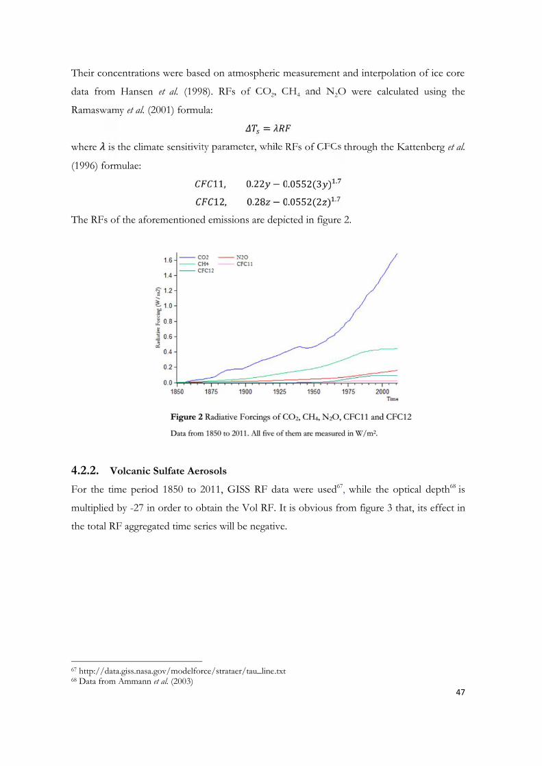
47
Their concentrations were based on atmospheric measurement and interpolation of ice core
data from Hansen et al. (1998). RFs of CO2, CH4 and N2O were calculated using the
Ramaswamy et al. (2001) formula: =where is the climate sensitivity parameter, while RFs of CFCs through the Kattenberg et al.
(1996) formulae: 11, 0.22 − 0.0552(3 ) .12, 0.28 − 0.0552(2 ) .The RFs of the aforementioned emissions are depicted in figure 2.
4.2.2. Volcanic Sulfate AerosolsFor the time period 1850 to 2011, GISS RF data were used67, while the optical depth68 is
multiplied by -27 in order to obtain the Vol RF. It is obvious from figure 3 that, its effect in
the total RF aggregated time series will be negative.
67 http://data.giss.nasa.gov/modelforce/strataer/tau_line.txt68 Data from Ammann et al. (2003)
Figure 2 Radiative Forcings of CO2, CH4, N2O, CFC11 and CFC12
Data from 1850 to 2011. All five of them are measured in W/m2.

48
4.2.3. Anthropogenic Sulfur EmissionsData from Smith et al. (2011) and Klimont et al. (2013) were used to create 1850 to 2011 time
series. The following formula is used to calculate the indirect RF:
= −0.13 − 0.87 ln 1 + ℎ26ln 1 + ℎ 26where is the annual anthropogenic sulfur emissions in Tg , and ℎ is the stack height term.
The 1990 direct and indirect RF values of are -0.42 and -1.0 respectively, while indirect
RF in 1850 is -0.17 . Natural and anthropogenic 1990 burden (mass in the atmosphere)
values are 0.19 and 0.47 Tg , respectively. These values were taken from Boucher and
Pham (2002). The anthropogenic sulfur emissions’ RF time series is depicted in figure 4.
Figure 3 Radiative Forcing of volcanic sulfate aerosols
Data from 1850 to 2011, measured in W/m2.
Figure 4 Radiative Forcing of Anthropogenic sulfuremissions
Data from 1850 to 2011, measured in W/m2.

49
4.2.4. Solar Irradiance, Black and Organic CarbonSolar irradiance time series were taken from Lean (2000), in which an index is created using
GISS website data, and were updated using Frohlich and Lean (1998) data. The resulting
time series includes 1850 to 2011 data, and the Sol RF is calculated using the Kattenberg et
al. (1996) formula. Black and organic carbon RF from 1850 to 2011, is provided in RCP 8.5
(Meinshausen et al. 2011).
Figure 5 Radiative Forcing of Solar Irradiance
Data from 1850 to 2011, measured in W / m2
-0.05
0.00
0.05
0.10
0.15
0.20
0.25
0.30
0.35
1850 1875 1900 1925 1950 1975 2000
RadiativeForcing(W/m2)
Time
Figure 6 Radiative Forcing of Black and Organic Carbon
Data from 1850 to 2011, measured in W / m2

50
CHAPTER 55. Empirical Application
In order to incorporate with specific uncertainties stemming from the relative size of black
carbon (BC) and anthropogenic sulfate emissions (S) RFs, four scenarios are created,
following Stern and Kaufmann (2014):
1st Scenario: the 1990 levels (baseline) of BC and S are used, as measured in Meinshausen et
al. (2011) and Boucher and Pham (2002). They are 0.31 W/m2 for BC and -
1.42 W/m2 for S, and this scenario is indicated as BC=1, S=1.
2nd Scenario: S is equal to its baseline level, while BC has no effect on global warming. This
scenario is indicated as BC=0, S=1.
3rd Scenario: S is equal to its baseline level, while BC has three times the baseline effect on
global warming. This scenario is indicated as BC=3, S=1.
4th Scenario: S has half the effect of its baseline level, while BC has no effect on global
warming. This scenario is indicated as BC=0, S=0.5.
-0.5
0.0
0.5
1.0
1.5
2.0
2.5
1850 1875 1900 1925 1950 1975 2000
RadiativeForcing(W/m2)
TimeFigure 7 Radiative forcing of Greenhouse GasesData are aggregated CO2, CH4, N2O and CFCs, from 1850 to 2011, measured in W /m2
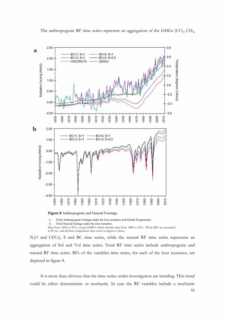
51
The anthropogenic RF time series represent an aggregation of the GHGs (CO2, CH4,
N2O and CFCs), S and BC time series, while the natural RF time series represents an
aggregation of Sol and Vol time series. Total RF time series include anthropogenic and
natural RF time series. RFs of the variables time series, for each of the four scenarios, are
depicted in figure 8.
It is more than obvious that the time series under investigation are trending. This trend
could be either deterministic or stochastic. In case the RF variables include a stochastic
b
a
Figure 8 Anthropogenic and Natural Forcings
a. Total Anthropogenic forcings under the four scenarios and Global Temperature.b. Total Natural forcings under the four scenarios.
Data from 1850 to 2011, except GISSv3 which includes data from 1880 to 2011. All the RFs are measuredin W/m2, and all three temperature time series in degrees Celsius.

52
trend, changes in them might also cause a stochastic trend in temperature. In order to
examine these possible relationships, causality testing should take place. But first, the nature
of the variables time series must be explored. That is determining whether the trending in
the variables is either deterministic or stochastic.
5.1. Stationarity Test ResultsThe widely used ADF, ADF–GLS, PP and KPSS stationarity tests are the used tools for
examining the time series properties of the variables. Results, presented in table 2, indicate
that anthropogenic RFs are I(1) for the first three scenarios in all but KPSS (which indicates
it to be I(2)) tests, while in the fourth scenario it is I(2) for all but PP. All tests show that
Natural RF is stationary, whereas Total, BC and S RFs as well as both Temperature time
series are I(1). Finally the GHGs RF is found to be I(2) in all tests. Total RF is stationary for
all scenarios in ADF-GLS and PP, as well as for all scenarios except the third one in ADF.
In this scenario in ADF, as well as in all scenarios in KPSS, the order of integration of the
total series is I(1). Vol appear to be stationary while ADF-GLS, PP and KPSS show that Sol
is I(1), and only ADF differentiates.
Table 2 Stationarity Test Results
Test ADF* ADF – GLS** PP* KPSS***Scenarios 1 2 3 4 1 2 3 4 1 2 3 4 1 2 3 4
Natural -7.21 (0) -6.74 (0) -5.70 (0) 0.16 (0)
Anthropogenic -3.23(1)
-3.05(1)
-3.94(1)
-15.49(2)
-2.86(1)
-2.82(1)
-3.27(1)
-15.54(2)
-7.35(1)
-6.92(1)
-7.65(1)
-4.93(1)
0.10(2)
0.09(2)
0.25(2)
0.08(2)
Total -3.21(0)
-3.61(0)
-12.58(1)
-2.88(0)
-3.21(0)
-3.63(0)
-2.27(0)
-2.76(0)
-4.01(0)
-4.43(0)
-3.26(0)
-3.69(0)
0.44(1)
0.47(1)
0.38(1)
0.39(1)
GHGs -8.41 (2) -8.35 (2) -22.29 (2) 0.04 (2)
BC -3.50 (1) -2.6 (1) -6.67 (1) 0.21 (1)
S -7.86 (1) -7.57 (1) -8.28 (1) 0.18 (1)
Vol -7.36 (0) -4.87 (0) -5.78 (0) 0.08 (0)
Sol -9.47 (2) -1.76 (1) -6.49 (1) 0.17 (1)
Temperature(GISS) -11.15 (1) -3.87 (1) -23.12 (1) 0.10 (1)
Temperature(HadCRUT4) -12.01 (1) I(1) -23.45 (1) 0.11 (1)
Ocean HeatContent -7.44 (1) -7.27 (1) -10.61 (1) 0.26 (1)

53
Notes: Numbers in parentheses are the order of integration of each variable’s time series for the 1850 to 2011 time period.All gases’ time series are expressed as RFs. BC stands for black carbon, S for anthropogenic sulfur emissions. Vol forvolcanic sulfate aerosols and Sol for solar irradiance. Total represents an aggregation of natural and anthropogenic RFs,natural of Vol and Sol, and anthropogenic of GHGs (CO2, CH4, N2O and CFCs), S and BC. The numeric values are t-statistics in the 5% significance level. Scenario 1: BC=1, S=1, scenario 2: BC=0, S=1, scenario 3: BC=3, S=1 and scenario4: BC=0, S=0.5. * Critical values are: 1% -3.47, 5% -2.87 and 10% -2.57. ** Critical values are: 1% -2.58, 5% -1.94 and 10%-1.61. *** Critical values are: 1% 0.73, 5% 0.46 and 10% 0.34.
Regarding the tests which follow, and for convenience, the order of integration of
each variable is assumed to be the one indicated by the majority of the stationarity tests,
presented in table 3. Anthropogenic time series in scenarios 1, 2 and 3 are regarded as I(1),
while it is I(2) in the fourth scenario. Black carbon, anthropogenic sulfur emissions, Sol,
GISSv3, HADCRUT4 and Ocean Heat Content time series, are assumed to be I(1), while
natural and total RFs are stationary. The GHGs RF time series is regarded as I(2).
Table 3 Order of Integration as indicated by the majority of the tests
Variable Natural Anthropogenic Total GHGs BC S Vol Sol GISSv3 HADCRUT4 OHC
Scenario 1 2 3 4 1 2 3 4
Order ofintegration 0 1 1 1 2 0 0 0 0 2 1 1 0 1 1 1 1
Notes: Numbers in table are the order of integration of each variable’s time series for the 1850 to 2011 time period, as indicated bythe majority of the stationarity tests. All gases’ time series are expressed as RFs. BC stands for black carbon, S for anthropogenicsulfur emissions, Vol for volcanic sulfate aerosols, Sol for solar irradiance and OHC for ocean heat content. Total represents anaggregation of natural and anthropogenic RFs, natural of Vol and Sol, and anthropogenic of GHGs (CO2, CH4, N2O and CFCs),S and BC. Scenario 1: BC=1, S=1, scenario 2: BC=0, S=1, scenario 3: BC=3, S=1 and scenario 4: BC=0, S=0.5.
5.2. Cointegration AnalysisIn order to set an econometric model and discover possible relationships between these
variables, the existence or not of a cointegrating relationship must first be examined.
Spurious results can be avoided through cointegration analysis.
5.2.1. Engle–Granger Cointegration Test ResultsThe long–run equilibrium relationship that is assumed to exist between I(1) variables,
described by equation (3.25), representing a possible linear combination between the
variables, is tested for cointegration. Due to limited data in specific variables’ time series,
three levels of aggregation are tested, through three Models. In Model I, total Anthropogenic
and Natural RFs are aggregated and subsequently fed in the cointegration test against
temperature. In Model II, total Anthropogenic and Natural RFs are fed separately in the test
against temperature. Finally, in Model III, all RFs (with GHGs being aggregated) are fed in
the test against temperature separately. The third Model cannot be used in an Engle and
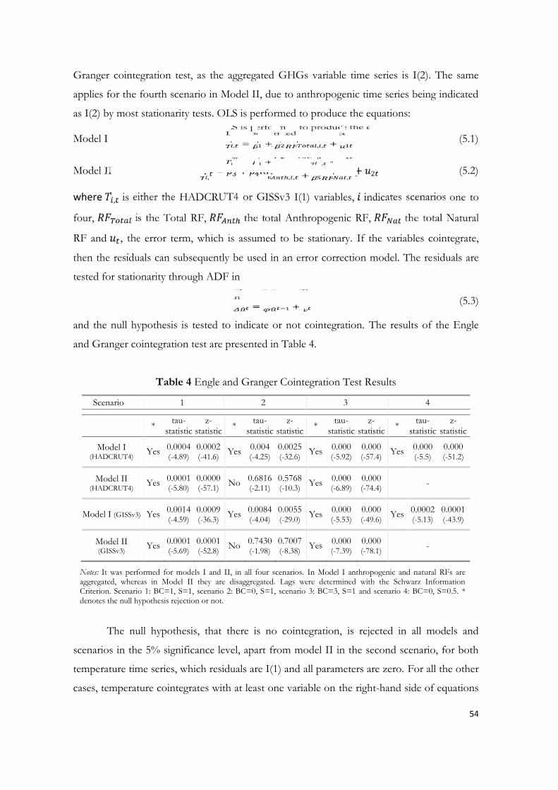
54
Granger cointegration test, as the aggregated GHGs variable time series is I(2). The same
applies for the fourth scenario in Model II, due to anthropogenic time series being indicated
as I(2) by most stationarity tests. OLS is performed to produce the equations:
Model I , = + , , + (5.1)
Model II , = + , , + , + (5.2)
where , is either the HADCRUT4 or GISSv3 I(1) variables, indicates scenarios one to
four, is the Total RF, the total Anthropogenic RF, the total Natural
RF and , the error term, which is assumed to be stationary. If the variables cointegrate,
then the residuals can subsequently be used in an error correction model. The residuals are
tested for stationarity through ADF in = + (5.3)
and the null hypothesis is tested to indicate or not cointegration. The results of the Engle
and Granger cointegration test are presented in Table 4.
Table 4 Engle and Granger Cointegration Test Results
Scenario 1 2 3 4
* tau-statistic
z-statistic * tau-
statisticz-
statistic * tau-statistic
z-statistic * tau-
statisticz-
statistic
Model I(HADCRUT4) Yes 0.0004
(-4.89)0.0002(-41.6) Yes 0.004
(-4.25)0.0025(-32.6) Yes 0.000
(-5.92)0.000(-57.4) Yes 0.000
(-5.5)0.000(-51.2)
Model II(HADCRUT4) Yes 0.0001
(-5.80)0.0000(-57.1) No 0.6816
(-2.11)0.5768(-10.3) Yes 0.000
(-6.89)0.000(-74.4) -
Model I (GISSv3) Yes 0.0014(-4.59)
0.0009(-36.3) Yes 0.0084
(-4.04)0.0055(-29.0) Yes 0.000
(-5.53)0.000(-49.6) Yes 0.0002
(-5.13)0.0001(-43.9)
Model II(GISSv3) Yes 0.0001
(-5.69)0.0001(-52.8) No 0.7430
(-1.98)0.7007(-8.38) Yes 0.000
(-7.39)0.000(-78.1) -
Notes: It was performed for models I and II, in all four scenarios. In Model I anthropogenic and natural RFs areaggregated, whereas in Model II they are disaggregated. Lags were determined with the Schwarz InformationCriterion. Scenario 1: BC=1, S=1, scenario 2: BC=0, S=1, scenario 3: BC=3, S=1 and scenario 4: BC=0, S=0.5. *denotes the null hypothesis rejection or not.
The null hypothesis, that there is no cointegration, is rejected in all models and
scenarios in the 5% significance level, apart from model II in the second scenario, for both
temperature time series, which residuals are I(1) and all parameters are zero. For all the other
cases, temperature cointegrates with at least one variable on the right-hand side of equations

55
5.1 and 5.2. In order to find the long-run coefficients, the cointegrating vector is estimated
through FM-OLS and a regression of the Error Correction Model is run.
5.2.2. Johansen Cointegration Test ResultsThe Johansen cointegration test involves the estimation of a VAR(k) model, with an optimal
lag length determined through the Schwarz Information Criterion. This is done through
selecting the lag length yielding the smallest value. The null hypothesis is that there is no
cointegrating relationship between temperature and the variables corresponding to the
Models. The third Model cannot be used in the Johansen cointegration test, as the
aggregated GHGs variable time series is I(2). The same applies for the fourth scenario in
Model II, due to anthropogenic time series being indicated as I(2) by most stationarity tests.
The Johansen cointegration test also reveals the number of such relationships between the
aforementioned variables. Thus, it consecutively tests:: = 0,: = 1: = 1,: = 2…
The trace statistics and p – values as well as the optimal lag length and number of
cointegrating relationships, as revealed by the Johansen cointegration test, are presented in
tables 5 and 6.
Table 5 Johansen Cointegration Test Results
Scenario 1 2 3 4
Tracestatistic p-value Trace
statistic p-value Tracestatistic p-value Trace
statistic p-value
Model I(HADCRUT4)
0: 46.5* 0.000 0: 44.0* 0.000 0: 49.1* 0.000 0: 50.3* 0.0001: 3.16 0.075 1: 3.18 0.074 1: 3.01 0.082 1: 3.12 0.077
Model II(HADCRUT4)
0: 54.2* 0.000 0: 45.4* 0.000 0: 97.8* 0.000-1: 22.2* 0.004 1: 13.5 0.096 1: 46.3* 0.000
2: 9.08* 0.002 2: 4.8* 0.028 2: 12.0* 0.000
Model I(GISSv3)
0: 23.3* 0.002 0: 21.4* 0.005 0: 26.5* 0.000 0: 26.5* 0.0001: 0.29 0.584 1: 0.31 0.577 1: 0.27 0.601 1: 0.29 0.585
Model II(GISSv3)
0: 45.5* 0.000 0: 38.8* 0.003 0: 84.2* 0.000-1: 17.8* 0.021 1: 11.2 0.197 1: 42.3* 0.000
2: 7.0* 0.008 2: 3.61 0.057 2: 8.8* 0.002
Notes: The Johansen cointegration test was performed for Models I and II in all four scenarios, for the 1850to 2011 time period. In Model I anthropogenic and natural RFs are aggregated, whereas in Model II they
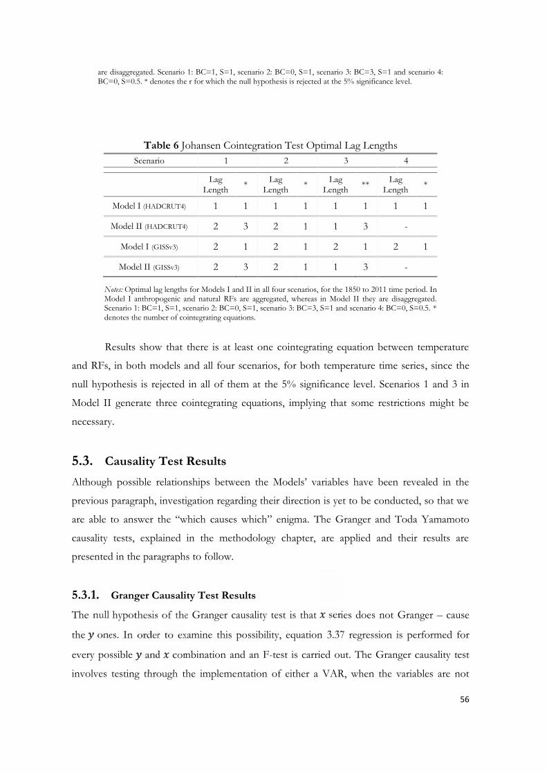
56
are disaggregated. Scenario 1: BC=1, S=1, scenario 2: BC=0, S=1, scenario 3: BC=3, S=1 and scenario 4:BC=0, S=0.5. * denotes the r for which the null hypothesis is rejected at the 5% significance level.
Table 6 Johansen Cointegration Test Optimal Lag LengthsScenario 1 2 3 4
LagLength * Lag
Length * LagLength ** Lag
Length *
Model I (HADCRUT4) 1 1 1 1 1 1 1 1
Model II (HADCRUT4) 2 3 2 1 1 3 -
Model I (GISSv3) 2 1 2 1 2 1 2 1
Model II (GISSv3) 2 3 2 1 1 3 -
Notes: Optimal lag lengths for Models I and II in all four scenarios, for the 1850 to 2011 time period. InModel I anthropogenic and natural RFs are aggregated, whereas in Model II they are disaggregated.Scenario 1: BC=1, S=1, scenario 2: BC=0, S=1, scenario 3: BC=3, S=1 and scenario 4: BC=0, S=0.5. *denotes the number of cointegrating equations.
Results show that there is at least one cointegrating equation between temperature
and RFs, in both models and all four scenarios, for both temperature time series, since the
null hypothesis is rejected in all of them at the 5% significance level. Scenarios 1 and 3 in
Model II generate three cointegrating equations, implying that some restrictions might be
necessary.
5.3. Causality Test ResultsAlthough possible relationships between the Models’ variables have been revealed in the
previous paragraph, investigation regarding their direction is yet to be conducted, so that we
are able to answer the “which causes which” enigma. The Granger and Toda Yamamoto
causality tests, explained in the methodology chapter, are applied and their results are
presented in the paragraphs to follow.
5.3.1. Granger Causality Test Results
The null hypothesis of the Granger causality test is that series does not Granger – cause
the ones. In order to examine this possibility, equation 3.37 regression is performed for
every possible and combination and an F-test is carried out. The Granger causality test
involves testing through the implementation of either a VAR, when the variables are not
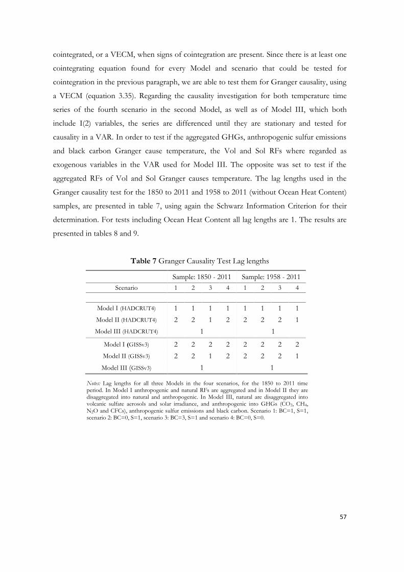
57
cointegrated, or a VECM, when signs of cointegration are present. Since there is at least one
cointegrating equation found for every Model and scenario that could be tested for
cointegration in the previous paragraph, we are able to test them for Granger causality, using
a VECM (equation 3.35). Regarding the causality investigation for both temperature time
series of the fourth scenario in the second Model, as well as of Model III, which both
include I(2) variables, the series are differenced until they are stationary and tested for
causality in a VAR. In order to test if the aggregated GHGs, anthropogenic sulfur emissions
and black carbon Granger cause temperature, the Vol and Sol RFs where regarded as
exogenous variables in the VAR used for Model III. The opposite was set to test if the
aggregated RFs of Vol and Sol Granger causes temperature. The lag lengths used in the
Granger causality test for the 1850 to 2011 and 1958 to 2011 (without Ocean Heat Content)
samples, are presented in table 7, using again the Schwarz Information Criterion for their
determination. For tests including Ocean Heat Content all lag lengths are 1. The results are
presented in tables 8 and 9.
Table 7 Granger Causality Test Lag lengths
Sample: 1850 - 2011 Sample: 1958 - 2011Scenario 1 2 3 4 1 2 3 4
Model I (HADCRUT4) 1 1 1 1 1 1 1 1Model II (HADCRUT4) 2 2 1 2 2 2 2 1Model III (HADCRUT4) 1 1
Model I (GISSv3) 2 2 2 2 2 2 2 2Model II (GISSv3) 2 2 1 2 2 2 2 1Model III (GISSv3) 1 1
Notes: Lag lengths for all three Models in the four scenarios, for the 1850 to 2011 timeperiod. In Model I anthropogenic and natural RFs are aggregated and in Model II they aredisaggregated into natural and anthropogenic. In Model III, natural are disaggregated intovolcanic sulfate aerosols and solar irradiance, and anthropogenic into GHGs (CO2, CH4,N2O and CFCs), anthropogenic sulfur emissions and black carbon. Scenario 1: BC=1, S=1,scenario 2: BC=0, S=1, scenario 3: BC=3, S=1 and scenario 4: BC=0, S=0.

58
Table 8 Granger Causality Test Results (HADCRUT4)
Sample 1850 – 2011 1958 – 2011 1958 – 2011 (with OHC)Scenario 1 2 3 4 1 2 3 4 1 2 3 4
Model I
T → Total 0.3949 0.5577 0.2037 0.2485 0.2748 0.3069 0.2258 0.2926 0.8370 0.9071 0.4373 0.9970
Total → T 0.3299 0.2157 0.6382 0.4988 0.9945 0.9033 0.8338 0.9474 0.3605 0.2648 0.5900 0.3090
Model II
N → T 0.2053 0.2334 0.0557 0.0446 0.2597 0.5836 0.1302 0.1090 0.0970 0.1971 0.1746 0.0499
T → A 0.0213 0.0267 0.0140 0.0573 0.5645 0.7861 0.2834 0.0063 0.3857 0.6145 0.2451 0.0282
A → T 0.4628 0.2982 0.3812 0.0792 0.0059 0.0386 0.0275 0.0007 0.0114 0.0468 0.0630 0.0099
Model III
GHGs → T 0.0001 0.0009 0.0160
S → T 0.1087 0.7474 0.9515
BC → T 0.8125 0.7887 0.7152
GHGs, S & BC → T 0.0002 0.0010 0.0011
Vol → T 0.3228 0.2086 0.1172
Sol → T 0.6502 0.4170 0.5130
Vol & Sol → T 0.5058 0.0935 0.0938
T → GHGs 0.0002 0.0001 0.0008
Notes: Numbers in the table are p values for each Model in the four scenarios. All gases’ time series are expressed as RFs.BC stands for black carbon, S for anthropogenic sulfur emissions, Vol for volcanic sulfate aerosols, Sol for solarirradiance, T for temperature, N for natural, A for anthropogenic and OHC for Ocean Heat Content. Total represents anaggregation of natural and anthropogenic RFs, natural of Vol and Sol, and anthropogenic of GHGs (CO2, CH4, N2O andCFCs), S and BC. In Model I anthropogenic and natural RFs are aggregated and in Model II they are disaggregated intonatural and anthropogenic. In Model III, natural are disaggregated into Vol and Sol, and anthropogenic into GHGs, S andBC. Scenario 1: BC=1, S=1, scenario 2: BC=0, S=1, scenario 3: BC=3, S=1 and scenario 4: BC=0, S=0.5.

59
Table 9 Granger Causality Test Results (GISSv3)
Sample 1850 – 2011 1958 – 2011 1958 – 2011 (with OHC)Scenario 1 2 3 4 1 2 3 4 1 2 3 4
Model I
T → Total 0.2930 0.3851 0.1703 0.1972 0.1669 0.1903 0.1308 0.1755 0.3711 0.7402 0.0957 0.3599
Total → T 0.5578 0.4706 0.6145 0.6163 0.9183 0.8155 0.9980 0.9194 0.1733 0.0891 0.4484 0.1788
Model II
N → T 0.2476 0.2575 0.1131 0.0352 0.1531 0.5540 0.0696 0.0995 0.1337 0.2520 0.1798 0.0449
T → A 0.0862 0.1156 0.0647 0.1456 0.7826 0.7899 0.5682 0.0095 0.6688 0.9348 0.4874 0.0297
A → T 0.4569 0.2748 0.3351 0.0873 0.2830 0.3786 0.3492 0.0019 0.3693 0.6080 0.4960 0.0206
Model III
GHGs → T 0.0009 0.0058 0.0585
S → T 0.0529 0.6354 0.8713
BC → T 0.9211 0.8908 0.7991
GHGs, S & BC → T 0.0016 0.0063 0.0022
Vol → T 0.2831 0.1808 0.0867
Sol → T 0.7501 0.5515 0.6869
Vol & Sol → T 0.3420 0.0608 0.0863
T → GHGs 0.0003 0.0002 0.0012
Notes: Numbers in the table are p values for each Model in the four scenarios. All gases’ time series are expressed as RFs.BC stands for black carbon, S for anthropogenic sulfur emissions, Vol for volcanic sulfate aerosols, Sol for solarirradiance, T for temperature, N for natural, A for anthropogenic and OHC for Ocean Heat Content. Total represents anaggregation of natural and anthropogenic RFs, natural of Vol and Sol, and anthropogenic of GHGs (CO2, CH4, N2O andCFCs), S and BC. In Model I anthropogenic and natural RFs are aggregated and in Model II they are disaggregated intonatural and anthropogenic. In Model III, natural are disaggregated into Vol and Sol, and anthropogenic into GHGs, S andBC. Scenario 1: BC=1, S=1, scenario 2: BC=0, S=1, scenario 3: BC=3, S=1 and scenario 4: BC=0, S=0.5.
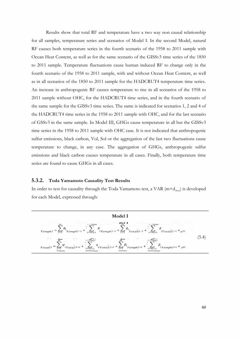
60
Results show that total RF and temperature have a two way non causal relationship
for all samples, temperature series and scenarios of Model I. In the second Model, natural
RF causes both temperature series in the fourth scenario of the 1958 to 2011 sample with
Ocean Heat Content, as well as for the same scenario of the GISSv3 time series of the 1850
to 2011 sample. Temperature fluctuations cause human induced RF to change only in the
fourth scenario of the 1958 to 2011 sample, with and without Ocean Heat Content, as well
as in all scenarios of the 1850 to 2011 sample for the HADCRUT4 temperature time series.
An increase in anthropogenic RF causes temperature to rise in all scenarios of the 1958 to
2011 sample without OHC, for the HADCRUT4 time series, and in the fourth scenario of
the same sample for the GISSv3 time series. The same is indicated for scenarios 1, 2 and 4 of
the HADCRUT4 time series in the 1958 to 2011 sample with OHC, and for the last scenario
of GSSv3 in the same sample. In Model III, GHGs cause temperature in all but the GISSv3
time series in the 1958 to 2011 sample with OHC case. It is not indicated that anthropogenic
sulfur emissions, black carbon, Vol, Sol or the aggregation of the last two fluctuations cause
temperature to change, in any case. The aggregation of GHGs, anthropogenic sulfur
emissions and black carbon causes temperature in all cases. Finally, both temperature time
series are found to cause GHGs in all cases.
5.3.2. Toda Yamamoto Causality Test ResultsIn order to test for causality through the Toda Yamamoto test, a VAR (m+dmax) is developed
for each Model, expressed through:
Model I
, = , + , + , + , +(5.4)
, = , + , + , + , +

61
Model II
, = , + , + + + ℎ , + ℎ , += , + , + + + ℎ , + ℎ , + (5.5)
ℎ , = , + , + + + ℎ , + ℎ , +Model IΙI
, = , + , + + + + ++ + + + + +
(5.6)
= , + , + + + + ++ + + + + +
= , + , + + + + ++ + + + + +
= , + , + + + + ++ + + + + +
= , + , + + + + + ℎ+ ℎ + + + + +
= , + , + + + + ++ + + + + +
where is the Temperature, ℎ is the anthropogenic, the anthropogenic sulfur
emissions, the black carbon, the volcanic sulfate aerosols, and the solar
irradiance RF. The optimal lag length is denoted with , is the maximum order of
integration of the variables in each Model, represents either HADCRUT4 or GISSv3,

62
represents scenarios one to four, and the error terms. The null hypothesis is that there no
causality between the variables, and the hypotheses that were tested can be expressed as:
Model I : = 0, ∀ = 1,2, … , : = 0, ∀ = 1,2, … ,Model II : = 0, ∀ = 1,2, … , : = 0, ∀ = 1,2, … , : = 0, ∀ = 1,2,… ,
Model III
: = 0, ∀ = 1,2, … , : = 0, ∀ = 1,2, … , : = 0, ∀ = 1,2, … ,: = = = 0,∀ = 1,2, … , : = 0, ∀ = 1,2, … , : = 0, ∀ = 1,2, … ,: = = 0, ∀ = 1,2, … , : = 0, ∀ = 1,2, … ,
The VAR lag length is the maximum order of integration of the variables in each model and
scenario, added to the optimal lag length. Optimal lag lengths can be seen in table 6, with the
difference that for Model III in the 1850 to 2011 sample, as well as for the fourth scenario in
Model II in the 1958 to 2011 sample, for both temperature series, it is 2. For tests including
Ocean Heat Content all optimal lag lengths are 1. The VAR lag lengths used in the Toda
Yamamoto causality test can be seen in table 10. The formula connecting the variables is
estimated through OLS and a Wald test is performed for each hypothesis. The resulting p
values are presented in tables 11 and 12.
Table 10 Toda Yamamoto Causality Test VAR Lag Lengths
Sample: 1850 - 2011 Sample: 1958 – 2011(without OHC)
Sample: 1958 – 2011(with OHC)
Scenario 1 2 3 4 1 2 3 4 1 2 3 4
Model I (HADCRUT4) 2 2 2 2 2 2 2 2 2 2 2 2Model II (HADCRUT4) 3 3 2 4 3 3 3 4 2 2 2 3Model III (HADCRUT4) 4 3 3
Model I (GISSv3) 3 3 3 3 3 3 3 3 2 2 2 2Model II (GISSv3) 3 3 2 4 3 3 3 4 2 2 2 3Model III (GISSv3) 4 3 3
Notes: Lag lengths for all three Models in the four scenarios, for the 1850 to 2011 time period. In Model Ianthropogenic and natural RFs are aggregated and in Model II they are disaggregated into natural andanthropogenic. In Model III, natural are disaggregated into volcanic sulfate aerosols and solar irradiance, andanthropogenic into GHGs (CO2, CH4, N2O and CFCs), anthropogenic sulfate emissions and black carbon.Scenario 1: BC=1, S=1, scenario 2: BC=0, S=1, scenario 3: BC=3, S=1 and scenario 4: BC=0, S=0.5.

63
Table 11 Toda Yamamoto Causality Test Results (HADCRUT4)
Sample 1850 – 2011 1958 – 2011 1958 – 2011 (with OHC)Scenario 1 2 3 4 1 2 3 4 1 2 3 4
Model I
T → Total 0.1840 0.2779 0.1080 0.1269 0.1588 0.1753 0.1439 0.1917 0.5891 0.6408 0.5220 0.6717
Total → T 0.0077 0.0144 0.0021 0.0035 0.0121 0.0151 0.0080 0.0151 0.0076 0.0103 0.0042 0.0097
Model II
N → T 0.0611 0.0671 0.0350 0.0367 0.0054 0.0194 0.0025 0.0044 0.0417 0.0438 0.0386 0.0460
T → A 0.0416 0.0242 0.0670 0.1149 0.3652 0.3603 0.3886 0.4648 0.2520 0.2152 0.3036 0.8350
A → T 0.5190 0.3376 0.2647 0.0434 0.2668 0.2615 0.3372 0.0083 0.1581 0.5024 0.1583 0.0039
Model III
GHGs → T 0.0018 0.0362 0.4238
S → T 0.3537 0.1421 0.0472
BC → T 0.8696 0.6518 0.4951
GHGs, S & BC → T 0.0355 0.1178 0.2533
Vol → T 0.0349 0.2235 0.0181
Sol → T 0.3667 0.2333 0.4810
Vol & Sol → T 0.0467 0.3012 0.0583
T → GHGs 0.0589 0.0418 0.2289
Notes: Numbers in the table are p values for each Model in the four scenarios. All gases’ time series are expressed as RFs.BC stands for black carbon, S for anthropogenic sulfur emissions, Vol for volcanic sulfate aerosols, Sol for solarirradiance, T for temperature, N for natural, A for anthropogenic and OHC for Ocean Heat Content. Total represents anaggregation of natural and anthropogenic RFs, natural of Vol and Sol, and anthropogenic of GHGs (CO2, CH4, N2O andCFCs), S and BC. In Model I anthropogenic and natural RFs are aggregated and in Model II they are disaggregated intonatural and anthropogenic. In Model III, natural are disaggregated into Vol and Sol, and anthropogenic into GHGs, S andBC. Scenario 1: BC=1, S=1, scenario 2: BC=0, S=1, scenario 3: BC=3, S=1 and scenario 4: BC=0, S=0.5.

64
Table 12 Toda Yamamoto Causality Test Results (GISSv3)
Sample 1850 – 2011 1958 – 2011 1958 – 2011 (with OHC)Scenario 1 2 3 4 1 2 3 4 1 2 3 4
Model I
T → Total 0.8469 0.9293 0.6840 0.7438 0.8683 0.9005 0.8190 0.8999 0.7181 0.7975 0.6021 0.7775
Total → T 0.0069 0.0137 0.0137 0.0019 0.0002 0.0004 0.0001 0.0003 0.0009 0.0015 0.0003 0.0011
Model II
Natural → T 0.0512 0.0565 0.0221 0.0283 0.0001 0.0008 0.0000 0.0000 0.0033 0.0050 0.0022 0.0017
T → A 0.1047 0.0697 0.1537 0.2836 0.3186 0.2997 0.4205 0.4767 0.1462 0.1399 0.1472 0.8462
A → T 0.5361 0.3306 0.3426 0.0818 0.1751 0.0796 0.5835 0.0352 0.9966 0.6320 0.9156 0.0222
Model III
GHGs → T 0.0022 0.1984 0.4238
S → T 0.1427 0.1683 0.0472
BC → T 0.5983 0.9241 0.4951
GHGs, S & BC → T 0.0217 0.3874 0.2533
Vol → T 0.0404 0.0416 0.0181
Sol → T 0.4335 0.3800 0.4810
Vol & Sol → T 0.0580 0.1123 0.0583
T → GHGs 0.0106 0.1858 0.2289
Notes: Numbers in the table are p values for each Model in the four scenarios. All gases’ time series are expressed as RFs.BC stands for black carbon, S for anthropogenic sulfur emissions, Vol for volcanic sulfate aerosols, Sol for solarirradiance, T for temperature, N for natural, A for anthropogenic and OHC for Ocean Heat Content. Total represents anaggregation of natural and anthropogenic RFs, natural of Vol and Sol, and anthropogenic of GHGs (CO2, CH4, N2O andCFCs), S and BC. In Model I anthropogenic and natural RFs are aggregated and in Model II they are disaggregated intonatural and anthropogenic. In Model III, natural are disaggregated into Vol and Sol, and anthropogenic into GHGs, S andBC. Scenario 1: BC=1, S=1, scenario 2: BC=0, S=1, scenario 3: BC=3, S=1 and scenario 4: BC=0, S=0.5.

65
Results show that total RF causes temperature in all Models, samples and scenarios,
while the opposite causal direction does not apply. Natural RF causes temperature in all
scenarios in the 1958 to 2011 sample, and in scenarios 3 and 4 in the 1850 to 2011 sample.
Temperature fluctuations resulting in human induced RF to change is indicated only in
scenarios 1 and 2 of the 1850 to 2011 sample. An increase in anthropogenic RF causes
temperature to rise merely in the fourth scenario of all samples for both HADCRUT4 and
GISSv3, apart from the GISSv3 1850 to 2011 sample, which shows no causal relationship in
all scenarios. GHGs cause temperature for both temperature time series in the 1850 to 2011
sample, as well as for the HADCRUT4 time series in the 1958 to 2011 sample without
Ocean Heat Content. Anthropogenic sulfur emissions movements cause temperature
changes only when Ocean Heat Content is included in the Model, in the 1958 to 2011
sample. Black carbon does not cause temperature in any case. The aggregation of GHGs,
anthropogenic sulfur emissions and black carbon causes both temperature time series only in
the 1850 to 2011 sample. Vol cause temperature in all but the HADCRUT4 time series in
the 1958 to 2011 sample. Sol does not cause temperature in any case. The aggregation of Vol
and Sol causes temperature only for the HADCRUT4 time series in the 1850 to 2011
sample. Temperature causes GHGs merely for the GISSv3 time series in the 1850 to 2011
sample, and the HADCRUT4 time series in the 1958 to 2011 sample.
5.3.3. Rolling Window ResultsAlthough testing for causality in all three models’ hypotheses and all four scenarios, through
Toda Yamamoto, indicates that results are possibly robust, the rolling window methodology
is appropriate in order to examine each hypothesis’ robustness in different points in time.
Toda Yamamoto tests are performed as before, with a window length of 100 and a step of
five observations, for the 1850 to 2011 sample, for both temperature time series and in all
Models and scenarios. The VAR lag lengths for each case are presented in table 13, and the
Toda Yamamoto causality test results on a rolling basis are depicted in figures 9, 10, 11 and
12.
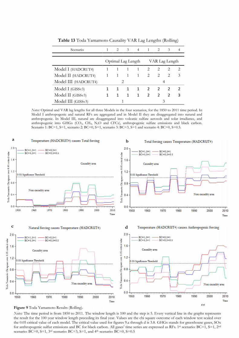
66
Table 13 Toda Yamamoto Causality VAR Lag Lengths (Rolling)
Scenario 1 2 3 4 1 2 3 4
Optimal Lag Length VAR Lag Length
Model I (HADCRUT4) 1 1 1 1 2 2 2 2Model II (HADCRUT4) 1 1 1 1 2 2 2 3Model III (HADCRUT4) 2 4
Model I (GISSv3) 1 1 1 1 2 2 2 2Model II (GISSv3) 1 1 1 1 2 2 2 3Model III (GISSv3) 1 3
Notes: Optimal and VAR lag lengths for all three Models in the four scenarios, for the 1850 to 2011 time period. InModel I anthropogenic and natural RFs are aggregated and in Model II they are disaggregated into natural andanthropogenic. In Model III, natural are disaggregated into volcanic sulfate aerosols and solar irradiance, andanthropogenic into GHGs (CO2, CH4, N2O and CFCs), anthropogenic sulfate emissions and black carbon.Scenario 1: BC=1, S=1, scenario 2: BC=0, S=1, scenario 3: BC=3, S=1 and scenario 4: BC=0, S=0.5.
a b
c d
Figure 9 Toda Yamamoto Results (Rolling).Notes: The time period is from 1850 to 2011. The window length is 100 and the step is 5. Every vertical line in the graphs representsthe result for the 100 year window length preceding its final year. Values are the chi square outcome of each window test scaled overthe 0.05 critical value of each model. The critical value used for figures 9.a through d is 3.8. GHGs stands for greenhouse gases, SOxfor anthropogenic sulfur emissions and BC for black carbon. All gases’ time series are expressed as RFs. 1st scenario: BC=1, S=1, 2nd
scenario: BC=0, S=1, 3rd scenario: BC=3, S=1, and 4th scenario: BC=0, S=0.5

67
Figure 10 Toda Yamamoto Results (Rolling).Notes: The time period is from 1850 to 2011. The window length is 100 and the step is 5. Every vertical line in the graphs represents the resultfor the 100 year window length preceding its final year. Values are the chi square outcome of each window test scaled over the 0.05 criticalvalue of each model. Critical values are: for 10.a is 3.8, for 10.b through d and 10.f is 6, and for 10.e is 9.5. GHGs stands for greenhouse gases,SOx for anthropogenic sulfur emissions and BC for black carbon. All gases’ time series are expressed as RFs. 1st scenario: BC=1, S=1, 2nd
scenario: BC=0, S=1, 3rd scenario: BC=3, S=1, and 4th scenario: BC=0, S=0.5
a
c
e
d
f
b

68
Figure 11 Toda Yamamoto Results (Rolling).Notes: The time period is from 1850 to 2011. The window length is 100 and the step 5. Every vertical line in the graphs represents the resultfor the 100 year window length preceding its final year. Values are the chi square outcome of each window test scaled over the 0.05 criticalvalue of each model. The critical value that was used for figures 11.a through e is 3.82, and for figure 11.f is 6. GHGs stands for greenhousegases, SOx for anthropogenic sulfur emissions and BC for black carbon. All gases’ time series are expressed as RFs. 1st scenario: BC=1, S=1,2nd scenario: BC=0, S=1, 3rd scenario: BC=3, S=1, and 4th scenario: BC=0, S=0.5
a b
dc
e f
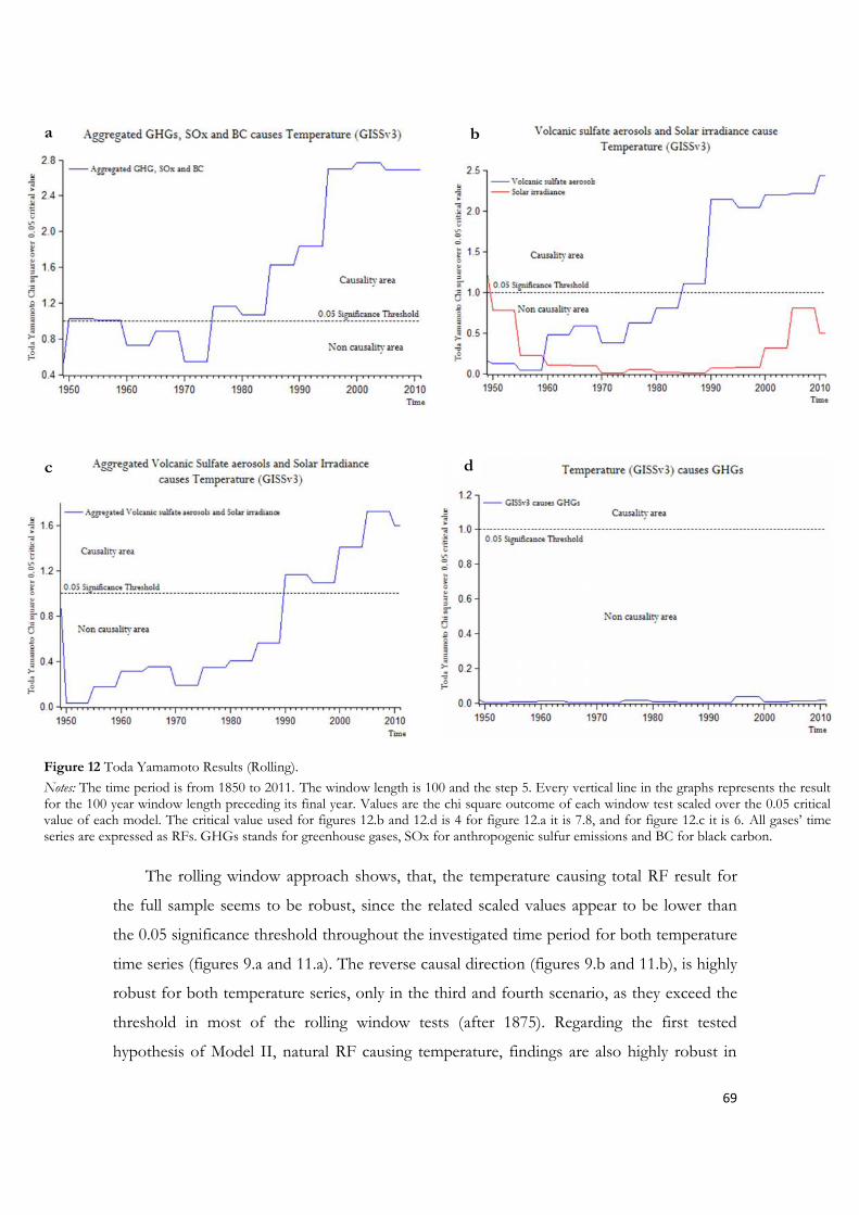
69
The rolling window approach shows, that, the temperature causing total RF result for
the full sample seems to be robust, since the related scaled values appear to be lower than
the 0.05 significance threshold throughout the investigated time period for both temperature
time series (figures 9.a and 11.a). The reverse causal direction (figures 9.b and 11.b), is highly
robust for both temperature series, only in the third and fourth scenario, as they exceed the
threshold in most of the rolling window tests (after 1875). Regarding the first tested
hypothesis of Model II, natural RF causing temperature, findings are also highly robust in
Figure 12 Toda Yamamoto Results (Rolling).Notes: The time period is from 1850 to 2011. The window length is 100 and the step 5. Every vertical line in the graphs represents the resultfor the 100 year window length preceding its final year. Values are the chi square outcome of each window test scaled over the 0.05 criticalvalue of each model. The critical value used for figures 12.b and 12.d is 4 for figure 12.a it is 7.8, and for figure 12.c it is 6. All gases’ timeseries are expressed as RFs. GHGs stands for greenhouse gases, SOx for anthropogenic sulfur emissions and BC for black carbon.
a b
c d

70
scenarios 1, 2 and 4, for both temperature time series (figures 9.c, 11.c). Temperature change
causing anthropogenic RF is robust for scenarios 3 and 4 of the HADCRUT4 results, which
showed no causal relationship between them in the full sample test, while all GISSv3 time
series scenarios’ results appear to be robust (figures 9.d, 11.d). Anthropogenic RF
fluctuations causing temperature change, for the HADCRUT4 time series results (figure
10.a), is robust in scenarios 1 and 3 and highly robust for the remaining two scenarios. Only
the first and third scenarios for the GISSv3 time series appear to be robust in the
anthropogenic climate change investigation of Model II (figure 11.e).
The black carbon and anthropogenic sulfur emissions’ changes leading in temperature
change results appear to be robust and GHGs’ fluctuations causing the temperature to
increase highly robust for the HADCRUT4 time series (figure 10.b). The same does not
apply for the aggregated result (figure 10.c). With reference to the GISSv3 time series (figure
11.f), Toda Yamamoto causality test results appear to be robust for anthropogenic sulfur
emissions and black carbon, and highly robust for GHGs, whereas the aggregated (GHGs,
BC and SOx) result is highly robust (figure 12.a). The Sol causing HADCRUT4 result is
robust throughout the investigated time period, whereas, the same does not apply for the
Vol (figure 10.d) and the aggregated RFs results (figure 10.e). The Sol and Vol individual
effects on GISSv3 are the same with the ones on HADCRUT4 (figure 12.b) , as well as the
aggregated RF causing GISSv3 causality result is highly robust for most of the tested
windows (figure 12.c). The HADCRUT4 causing GHGs result is robust, but this is not the
case for the GISSv3 time series (figures 10.f, 12.d).

71
CHAPTER 66. Discussion
In this chapter, the main findings of this dissertation are interpreted and discussed, in terms
of the rationale behind the choice of the implemented tests and their outcome’s validity, the
connection with literature and theory, as well as problems which have emerged and possible
solutions. Section one returns to the findings of chapter 5, regarding the time series under
review nature, that was explored in paragraph 1, and section two to the cointegration analysis
results of paragraph 2. Section three returns to the causality investigation explored in
paragraphs 3.1 and 3.2, and the robustness of the findings in these two paragraphs, as
explored in paragraph 3.3, are discussed in section four.
Section 1Several parameters regarding the Earth’s climate system, involving its orbital configuration,
continent movements etc., which affect global temperature in the long-run, are not taken into
consideration, and are considered external to the climate system, following most of the
related studies’ approach on the matter. Nevertheless, these parameters could be specified if
paleoclimate data were used, so that their long term effects are accounted for. The visual
inspection of the time series used in this dissertation, beginning in 1850, in chapter 4, resulted
in the observation that they are trending. These trends were subsequently identified in
chapter 5 (par.1), using stationarity testing, since stochastic trends in specific “suspicious”
gases’ time series, might cause a similar one in temperature time series. The fact that most of
the variables are found not to be stationary indicates that a relationship between them and
temperature could be found, and should be investigated further, since trends in time series
can act as fingerprints. Furthermore, the theory behind anthropogenic climate change begins
with the investigation of whether human induced emissions’ time series include stochastic
trends. Thus, such characterization of the variables’ time series, is the first step in answering
the question of whether natural, anthropogenic, as well as individual RFs are able to
influencing temperature, with a special interest in the human induced ones. Oscillations were
not included in the reasons behind temperature change, following Stern and Kaufmann
(2014). However, it is possible that anthropogenic and natural RFs affect them, so they could
be included in the temperature time series.
The four, most commonly used in the related literature, stationarity tests were
implemented. They showed that such stochastic trends are indeed present in anthropogenic

72
emissions’ time series, and this can also be supported through them being associated with
economic, population and policy changes, clearly connected with human activity. Such
activity was abruptly enhanced with the industrial revolution, marking the point in history
when global climate began to alter. The temperature, anthropogenic sulfur emissions, Sol
and GHGs time series stationarity test results are consistent with Stern and Kaufmann
(1997; 1997a; 1999; 2000; 2002; 2006a), regarding their non-stationary nature. Although, the
statistical power of stationarity tests is questionable, due to their low accuracy in detecting
real unit roots and ADF’s problematic behavior when brakes are included in data, the
application of more than two stationarity tests increases the accuracy of the results, despite
the individual test flaws. Regarding the time series length that was tested, instrumental
records might not be adequate to form the bigger picture of the variables’ evolution. Proxies
could help building an expanded set, improving our data and generating more accurate
stationarity test results. Other approaches could also be followed, regarding the time series
properties of the variables in the same scenarios, involving seasonality (cycles) being taken
into consideration, investigation through a fractional integration view, and a rolling window
method.
Section 2The identified trends in the variables can be matched with cointegration investigation. The
existence of more than one cointegrating relationships between the explanatory variables and
climate change indicators, in most of the hypothesis that were examined, as indicated by the
two tests that were performed, validates the suspected bond between them, as the
fingerprints, mentioned in section 1, prove to be present in both sides of these relationships.
Data limitations explain the rationale behind the Model specifications; consequently, three
levels of aggregation ought to be tested, enabling us to compare direct and indirect approach
results. The black carbon and anthropogenic sulfur emissions’ uncertain relative size, as
indicated through various studies (Forster et al. 2007; Bond et al. 2013), have also led to four
scenarios, depending on their 1990 values. Year 1958 marks the date when CO2 data started
being collected more meticulously, thus two sample sizes are tested (1850 to 2011 and 1958
to 2011), along with one including OHC in the 1958 to 2011 sample, since heat stored in
oceans might better describe the actual Temperature Model. Moreover, all Models, scenarios
and sample sizes are tested for both HADCRUT4 and GISSv3, as a robustness check.
Testing Models I and II for cointegration, which were the most aggregated ones, in scenarios

73
1,2 and 3, provided a straightforward result, indicating that relationships between total,
anthropogenic and natural RF with global temperature do exist, as expected, and their
direction should be investigated further through causality testing. Results are consistent with
most of the studies’, which support the anthropogenic climate change theory validity and
were described in the literature review chapter, outcomes. Nevertheless, scenario 4 of Model
II, as well as Model III, include variables of higher than the appropriate one for the
cointegration tests used in the analysis, order of integration, resulting in them not being
tested. A cointegrating relationship is assumed not to exist for them, for the rest of the
analysis, in order not to reach any biased outcome. However, the possible different result
when the opposite assumption is presumed, is examined in Appendix C. This problem could
be dealt with, using a modified VAR in a parameterization convenient for I(2) analysis, as
suggested in Johansen (1997).
Although the implementation of two cointegration tests in the analysis that was
performed in the empirical chapter, amplifies the outcome’s validity, the tools that were used
do not come without limitations. Despite the Engle and Granger cointegration test ease of
use, since ADF testing is involved, all its problems are also inherited, meaning that any error
introduced by ADF is carried over to the cointegration test outcome. A second disadvantage
emerges through the assumed existence of one cointegrating vector, as this can cause
problems when more than two variables are involved. Nevertheless, since the two Models
that were practically able to be analysed using this test, do not exceed this limit, this problem
is probably irrelevant in our case. However, another problematic behavior could have
affected the implemented analysis, as Engle and Granger performs naturally on large sample
sizes. The Phillip and Ouliaris (1990), Johansen (1991) and Watson maximum likelihood
estimator tests constitute ways of overcoming these Engle and Granger limitations.
Notwithstanding, the Johansen cointegration method also bears the limitation stemming
from the assumption that the cointegrating vector does not change with time. A method to
overcoming this problem could be the Gregory and Hansen (1996) suggestion, which takes
into account unknown structural breaks.
Section 3There exist several natural phenomena, feedbacks and anthropogenic sources that influence
global or regional temperature, in either a theoretical or proven sense, whose magnitude is
extensively researched in all cases. Even though it is not part in this dissertation’s area of

74
interest, an example of such natural phenomena impacting climate change, is the El Nino-
Southern Oscillation (ENSO). Surface Air Temperature (SAT) fluctuations result in the
periodical El Nino and La Nina phases that in turn affect weather, due to the rise or fall of
temperature, respectively. Similar relationships exist between temperature and other natural
phenomena as well. In addition, according to NASA, 69 temperature increase can create,
besides extreme hot weather, natural disasters, such as large changes in the density and
frequency of droughts, storms and hurricanes. These changes in humidity, along with
warming, enable air particles to sustain additional moisture, which leads to a positive
feedback, involving water vapor in the atmosphere to hold even more heat. Although human
activity does not directly affect water vapor in the atmosphere, our interference with methane
concentration can indirectly cause such an outcome. Another feedback in this category is the
albedo, or the surfaces’ ability to reflect light. Such snow and ice-related abilities are high,70
but, as temperature increases, it gets lower, resulting in more heat getting trapped in the
earth’s atmosphere. Nevertheless, there is also negative feedback, as of these of ocean and
land carbon cycles, which involves their ability to absorb carbon dioxide. Notwithstanding
oceans and land absorb carbon dioxide; warming can force them to reach their capacity and
start releasing it, counterbalancing the positive effect. Obviously, there are huge uncertainties
in regard to climate feedback, such as the cloud formations, methane hydrates and
permafrost methane responses to global warming. GHGs released into the atmosphere also
absorb solar radiation, increasing temperature. Their pre-industrial concentration levels
appear to have been substantially lower than today, initiating consensus about the
anthropogenic effect on global warming.
Some of the relationships, either speculative or not, described above, were
investigated in paragraphs 3.1 and 3.2. Since several problems arise with the implementation
of Granger causality test, such as, the possibility that it provides spurious results and
incorrect inference, along with F-test becoming invalid unless the variables are cointegrated,
the Toda Yamamoto approach was additionally used, for which integrated variables and non
cointegration do not affect the outcome. Causality test findings suggest that total, natural and
anthropogenic (in the fourth scenario) RFs cause temperature to change. The general idea is
that RFs are capable of affecting the ingoing and outgoing radiation energy balance, which,
at least to some extent, is believed to have increased after the industrial revolution, especially
through human contribution, since natural causes are expected to follow specific standard
69 http://earthobservatory.nasa.gov/70 Amounting for up to 30% of the total radiation entering the atmosphere, along with cloud formations.
75
patterns. Thus, results regarding total, natural and anthropogenic RFs’ relationships with
temperature, appear to be what were theoretically expected, and are consistent with Stern
and Kaufmann (2014). What is interesting is that the anthropogenic theory is better
described through the fourth scenario, where black carbon’s effect is null and anthropogenic
sulfur emissions’ is half its 1990 value. Reasons behind uncertainties regarding the black
carbon effects on climate, vary from the simple one, yet important, of which substances can
be described by the “black carbon” term, resulting in confusion in the related studies, to the
observational record’s deficiency, altitude implications, its interactions with clouds and ice
and underestimation of its energy and biomass related emissions’ magnitude (Bond et al.
2013). The anthropogenic sulfur emissions uncertainties stem from changes in the size, state,
shape and chemical composition of such gases when mixed with aerosols (Jacobson, 2001),
and the same also applies for black carbon (Chung and Seifeld, 2002).
A direct approach ought to be investigated as well, such as that of Model III, where
most gases are disaggregated, and results vary. As regards the GHGs’ contribution to global
warming, it is found to cause temperature, as expected, consistent with the Stern and
Kaufmann (2014) findings. Their concentration levels appear to have been substantially
affected by anthropogenic activity, as GHGs appear to follow an upward trend since the
industrial era (depicted in figure 15 of Appendix D). Contradictory to Stern and Kaufmann
(2014), it appears that anthropogenic sulfur emissions do not cause temperature to change.
This disagreement could have been a result of the slightly different approach in the Toda
Yamamoto causality test. Stern and Kaufmann (2014) use in this test the method of
seemingly unrelated regressions estimator (SUR), in which the error terms of the individual
regression equations are correlated. SUR is an approach to causality investigation which
requires researchers to be experienced, and can be used in future, related to this dissertation,
studies. Nevertheless, all other relationships of Model III result in the same to Stern and
Kaufmann (2014) outcomes, making the aforementioned discrepancy less alarming.
Section 4Although a robustness check was performed through multiple stationarity, cointegration and
causality tests in various samples, for two temperature data sets, additional research is
performed in the time domain, in order to assess the individual Models’ stability, since it is
possible that the associated parameters to change over time. The rolling window method
outcomes were mostly consistent with the related theory, as natural, anthropogenic, total,
76
solar irradiance and GHGs RFs causing temperature to change results, were found to be
highly robust for both temperature time series. The derived volcanic sulfate aerosols, along
with the human induced equivalent, robustness relationships with temperature being
inconclusive, might have more properly been examined when larger data sets are used, due
to the irregular occurrence of volcanic eruptions and the socioeconomic influence on
human behavior. The latter could also be examined taking into account present policy and
economic changes, which might explain future temperature fluctuation observations.
Consequently, these relationships could have been studied producing clearer and more
definite outcomes, in case the problem of inertia could practically be bypassed. Naturally,
climate, ecological and socioeconomic systems’ inertia does not allow for the anthropogenic
impacts on climate to neither instantly become apparent nor moderated. The atmospheric
lifetime of each pollutant is the basic reason behind the aforementioned statement. The
effects of carbon dioxide in particular will continue to influence global temperature (in the
magnitude of a fraction of a degree celsius per century) for at least a century past the point in
time when pollution seases (see figure 15 in Appendix D). A similar desynchronization is
present in ecosystems, where different flora and fauna species response times to
environmental changes are not the same, resulting in releasing or absorbing carbon dioxide
in various time points, leading to a disrupted carbon cycle. By all means, socioeconomic
interactions are also an important factor for this asynchrony, since policy implementation,
infrastracture, technology, economy and values play a big role. In addition, Kaufmann (2011)
results indicate that the anthropogenic sulfur emissions, volcanic sulphate aerosols, GHGs
and solar irradiance temperature influencies during the last couple of decades, seem to cancel
each other out (figures 3,4, and 5), resulting in the observed temperature increase hiatus.
According to the same author, a similar event fell within the 1940 to 1970 time period as
well. Thus, the simultaneous occurrence of increased sulfur polution rate (producing an
increased cooling effect), along with the transition from the El Nino to the La Nina phase
and a rise in solar irradiance, could constitute the reason behind the non unanimous causal
behavior along time.
77
CHAPTER 77. Conclusions
The purpose of this dissertation was to examine the robustness of the work of Stern and
Kaufmann (2014), using the same data, sample periods, Models and scenarios, as in the
aforementioned study. To accomplish this goal, the empirical analysis of the causal
relationships between radiative forcings of the most influencing gases known to date, with
temperature fluctuation indicators (HADCRUT4 and GSSv3) were explored, through the
implementation of stationarity, cointegration and causality testing. An extensive literature
review of climate change studies provided the necessary overview on the evolution of means
used leading to the respective findings. The novelty of this study is the causal relationship
investigation between two temperature time series and three Models in four scenarios,
describing three levels of aggregation in four cases due to uncertainty in the relative size of
specific gases, and its evolution over time through a rolling window method. The overall
findings suggest that natural, anthropogenic (in the fourth scenario) and total radiative
forcings cause temperature to change, and that these results are highly robust throughout the
sample period. The result of GHGs’ radiative forcing causing temperature change is
considerably robust, whereas it is inconclusive if the same applies for the volcanic sulfate
aerosols one. The effect of anthropogenic sulfate aerosols on temperature is robust merely
for the HADCRUT4 time series, solar irradiance not causing temperature change is across all
specifications, while their aggregated influence on temperature is only for the GISSv3 time
series. It is strongly indicated that temperature change causes GHGs concentrations
fluctuations, regardless of the sample under review, and this is robust for the HADCRUT4
time series (related further investigation is performed in Annex B). Final conclusions are
drawn based on the discussion and interpretation of this study’s findings in chapter 6, and
research questions, as were formulated in the introduction chapter, are answered.
Causality test findings of both direct and indirect Models, suggest that total, natural and
anthropogenic (in the fourth scenario) radiative forcings cause temperature to change.
Although it appears that there is not a unanimous answer as regards the individual forcings’
effects on temperature, results are mostly consistent with theory. That is that, when GHGs
78
rise, in particular, which are largely human related gases, it is suggested that they cause
temperature to increase, especially after the period of industrial revolution, supporting the
anthropogenic climate change theory. Furthermore, results show that a two way GHGs –
temperature causal relationship probably exists. Except for the human induced sulfur
emission relationship with temperature, all other findings are consistent with the respective
Stern and Kaufmann (2014) findings. Nevertheless, the aforementioned study is skeptic
about the anthropogenic sulfur emissions’ effects’ size, commenting that it “may be only
around half that usually attributed to them,” allowing the benefit of the doubt to penetrate.
Reasons behind outcome differences are possibly linked to a slightly alternative approach to
the causality tests used. Natural, anthropogenic, total, solar irradiance and GHGs radiative
forcings causing temperature to change results, were found to be highly robust, for both
temperature time series, throughout time. Volcanic sulfate aerosols and human induced
sulfur emissions’ results, through the time domain, were inconclusive, most likely due to data
set restrictions, socioeconomic influences and inertia. Problems related to the statistical
power of stationarity tests or their behavior to brakes in the time series could be dealt with
through seasonality, fractional integration and rolling window investigations. Paleoclimate
data could also help more accurately describe data evolution. Future work might also use
parameterization convenient for data series of higher order of integration in cointegration
analysis, since climate systems are described through variables’ sets, including such time
series. Unknown structural brakes, problems which might arise from taking for granted that
cointegrating vectors do not change over time and inertia should also be addressed.
Although future work could help expanding the outcome’s accuracy, this dissertation
provided an overall investigation, through various scenarios and Models, in order to augment
the work of Stern and Kaufmann (2014), exploring climate change causal relationships’
evolution through time, using all the available means that practically could have been. The
anthropogenic climate change theory is studied extensively and will probably linger in the air,
for as long as we systematically pollute this medium and consequently, our home. As it
appears, we have indeed already altered our environment, and will continue to affect it unless
a global effort is made to moderate the effects and slow our planet’s decay.

79
References
Adcock, R.J. (1878). A problem in Least Squares. Analyst 5, 53.
Akaike, H. (1973). Information theory and an extension of the maximum likelihood principle. In: Petrov, B.N., Csaki,F. (eds.). 2nd International Symposium on Information Theory. Akademini Kiado, Budapest, 267–281.
Allen, R.J., N. Nicholls, P.D. Jones and I.J. Butterworth (1991). A further extension of the Tahiti- Darwin SOI, earlySOI results and Darwin pressure. Journal of Climate 4, 743–749.
Allen, M.R. and S.F.B. Tett (1999). Checking for model consistency in optimal fingerprinting. Climate Dynamics 15,419–434.
Allen, M., N. Gillett, J. Kettleborough, G. Hegerl, R. Schnur, P. Stott, G. Boer, C. Covey, T. Delworth, G. Jones, J.Mitchell and T. Barnett (2006). Quantifying anthropogenic influence on recent near-surface temperature change.Surveys in Geophysics 27(5), 491-544.
Ammann, C.M., G.A. Meehl, W.M. Washington and C.S. Zender (2003). A monthly and latitudinally varying volcanicforcing data set in simulations of 20th century climate. Geophysical Research Letters 30 (12), 1657.
Andreou, A. and A. Spanos (2003). Statistical adequacy and the testing of trend versus difference stationary. EconomicReview 22, 217–237.
A.S.L. and Associates (1997). Sulfur Emissions by Country and Year. Report No. DE96014790, U.S. Department ofEnergy, Washington D.C.
Bangash, R.F., A. Passuello, M. Sanchez-Canales, M. Terrado, A. Lopez, F.J. Elorza, G. Ziv, V. Acuna and M.Schuhmacher (2013). Ecosystem services in Mediterranean river basin: Climate change impact on waterprovisioning and erosion control. Science of the Total Environment, 246–255.
Barnett, T.P., K. Hasselmann, M. Chelliah, T. Delworth, G. Hegerl, P. Jones, E. Rasmusson, E. Roeckner, C.Ropelewski, B. Santer and S. Tett (1999). Detecting and Attributing of Recent Climate Change: A Status Report.Bulletin of the American Meteorological Society 80(July), 2631–2659.
Battle, M., M. Bender, T. Sowers, P.P. Tans, J.H. Butler, J.W. Elkins, J.T. Ellis, T. Conway, N. Zhang, P. Lang and A.D.Clarke (1996). Atmospheric Gas Concentrations over the Past Century Measured in Air from Firn at the SouthPole. Nature 383, 231–235.
Beenstock, M., Y. Reingewertz and N. Paldor (2012). Polynomial cointegration tests of anthropogenic impact on globalwarming. Earth System Dynamics 3(2), 173–188.
Benkovitz, C. (1982). Compilation of an inventory of anthropogenic emissions in the United States and Canada.Atmospheric Environment 16, 1551–1563.
Berger, A.L. (1978). Long-term variations of daily insolation and quaternary climatic. Journal of Atmospheric Science 35(12),2362–2367.
Bloomfield, P. and D. Nychka (1992). Climate spectra and detecting climate change. Climatic Change 21, 275–287.
Boer, G.J., G. Flato, M.C. Reader and D.A. Ramsden (2000). Transient climate change simulation with greenhouse gasand aerosol forcing: experimental design and comparison with the instrumental record for the 20th century.Climate Dynamics 16, 405–425.
Bond, T.C., S.J. Doherty, D.W. Fahey, P.M. Forster, T. Berntsen, B.J. DeAngelo, M.G. Flanner, S. Ghan, B. Karcher,D. Koch, S.inne, Y. Kondo, P.K. Quinn, M.C. Sarofim, M.G. Schultz, M. Schulz, C. Venkataraman, et al. (2013).Bounding the role of black carbon in the climate system: a scientific assessment. Journal of Geophysical Research-Atmosphere, 118(11), 5380–5552.
Boucher, O. and M. Pham (2002). History of sulfate aerosol radiative forcings. Geophysical Research Letters 29(9), 1308.
Briffa, K.R. and P.D. Jones (1993). Global surface air temperature variations during the twentieth century: Part 2,implications for large-scale high-frequency paleoclimatic studies. The Holocene 3, 77-88.

80
Brohan, P., J.J. Kennedy, I. Harris, S.F.B. Tett and P.D. Jones (2006). Uncertainty estimates in regional and globalobserved temperature changes: A new dataset from 1850. Journal of Geophysical Research 111, D12106.
Chung, S.H. and J.H. Seinfeld (2002) Global distribution and climate forcing of carbonaceous aerosols. Journal ofGeophysical Research, 107, doi:10.1029/ 2001JD001397.
Collins, W., D. Stevenson, C. Johnson and R. Derwent (1997). Tropospheric ozone in a global-scale three-dimensionalLagrangian model and its re- sponse to NOx emission controls. Journal of Atmospheric Chemistry 26, 223–274.
Covey, C., K.M. Achutarao, U. Cubasch, P. Jones, S.J. Lambert, M.E. Mann, T.J. Phillips and K.E. Taylor (2003). Anoverview of results from the Coupled Model Intercomparison Project. Global and Planetary Change 37(1-2), 103–133.
Crowley, T.J. (2000). Causes of climate change over the past 1000 years. Science 289, 270–277.
Cubasch, U., K. Hasselmann, H. Hock, E. Maier-Reimer, U. Mikolajewicz, B.D. Santer and R. Sausen (1992). Time-dependent greenhouse warming computations with a coupled ocean-atmosphere model. Climate Dynamics 8, 55-69.
Cubasch, U., B.D. Santer, A. Hellbach, G. Hegerl, H. Hock, E. Maier-Reimer, U. Mikolajewiez, A. Stossel and R. Voss(1994). Monte Carlo climate change forecasts with a global coupled ocean-atmosphere model. Climate Dynamics10(1-2), 1–19.
Cubasch, U., G.C. Hegerl, A. Hellbach, H. Hock, U. Mikolajewicz, B.D. Santer and R. Voss (1995). A climate changesimulation starting from 1935. Climate Dynamics 11, 71-84.
Cubasch, U. and G.A. Meehl (2001). Projections of future climate change. In J. Houghton, (eds). Climate Change 2001:The scientific basis. Contribution of working group I of the third assessment Report of the Intergovernmental Panel on ClimateChange. Cambridge University Press, 526 - 582.
Cunnold, D., P. Fraser, R. Weiss, R. Prinn, P. Simmonds, B. Miller, F. Alyea and A. Crawford (1994). Global Trendsand Annual Releases of CCl3F and CCl2F2 Estimated from ALE/GAGE and Other Measurements from July 1978to June 1991. Journal of Geophysical Research 99 (D1), 1107–1126.
Cusack, S., J.M. Edwards and J.M. Crowther (1999). Investigating k distribution methods for parameterizing gaseousabsorption in the Hadley Centre climate model. Journal of Geophysical Research 104, 2051–2057.
Dickey, D. and W. Fuller (1979). Distribution of Estimators for Autoregressive Time Series with a Unit Root. Journal ofthe American Statistical Association 74(366), 427–431.
Dignon, J. and S. Hameed (1990). Global emissions of nitrogen and sulfur oxides from 1860 to 1980. Journal of AirPollution Control Association 39, 180–186.
Diebold, F.X. and R.S. Mariano (1995). Comparing predictive accuracy. Journal of Business and Economic Statistics 13, 253–263.
Dlugokenchy, E.J., P.M. Lang, K.A. Masarie and L.P. Steele (1994). Global CH4 Record from the NOAA/CMDL AirSampling Network. In Boden, T. A., D.P. Kaiser, R.J. Sepanski and F.S. Stoss, (eds.), Trends ’93: A Compendium ofData on Global Change, ORNL/CDIAC-65. Carbon Dioxide Information Analysis Center, Oak Ridge NationalLaboratory, Oak Ridge, TN, USA, 262–266.
Edwards, J.M. and A. Slingo (1996). Studies with a flexible new radiation code, I, Choosing a configuration for a large-scale model. Qouarterly Journal of the Royal Meteorological Society 122, 689–719.
Elliott, G., T.J. Rothenberg and J.H. Stock (1996). Efficient tests for an autoregressive unit root. Econometrica 64, 813–836.
Engle, R.F. and C.W.J. Granger (1987). Co-integration and error correction: representation, estimation and testing.Econometrica 55, 251–276.
Enting, I.G., H. Heimann and T.M.L. Wigley (1994). Future emissions and concentrations of carbon dioxide: keyocean/atmosphere/ land analyses. Technical Report 31, Commonwealth Scientific and Industrial ResearchOrganisation, Division of Atmospheric, Melbourne, Australia.

81
Etheridge,D.M., G.I. Pearman and P.J. Fraser (1994). Historical CH4 Record from the “DE08” Ice Core at Law Dome.In Boden, T. A., D.P. Kaiser, R.J. Sepanski and F.S. Stoss, (eds.), Trends ’93: A Compendium of Data on Global Change,ORNL/CDIAC-65. Carbon Dioxide Information Analysis Center, Oak Ridge National Laboratory, Oak Ridge,TN, USA, 256–260.
Etheridge, D.M., L.P. Steele, R.L. Langenfelds, R.J. Francey, J.M. Barnola and V.I. Morgan (1996). Natural andAnthropogenic Changes in Atmospheric CO2 over the Last 1000 Years from Air in Antarctic Ice and Firn. Journalof Geophysical Research 101, 4115–4128.
Folland, C.K., T.R. Karl and K.Ya, Vinnikov (1990). Observed Climate Variations and Change. In J.T. Houghton et al.(eds.), Climate Change: The IPCC Scientific Assessment, Cambridge University Press, 195-238.
Folland, C.K., T.R. Karl, N. Nicholls, B.S. Nyenzi, D.E. Parker and K.Y. Vinnikov (1992). Observed climate variabilityand change. In Houghton, J.T., B.A. Callander and S.K. Varney (eds.), Climate Change 1992. The Supplementary Reportto the IPCC Scientific Assessment. Cambridge University Press, Cambridge, UK, 135-170.
Forster, P., V. Ramaswamy, P. Artaxo, T. Berntsen, R. Betts, D.W. Fahey, J. Haywood, J. Lean, D.C. Lowe, G. Myhre,J. Nganga, R. Prinn, G. Raga, M. Schulz and R. Van Dorland (2007). Changes in atmospheric constituents and inradiative forcing. In: Solomon S., D. Qin, M. Manning, Z. Chen, M. Marquis, K.B. Averyt, M. Tignor, H.L. Miller(eds.) Climate change 2007: The physical science basis, Contribution of Working Group I to the FourthAssessment Report of the Intergovernmental Panel on Climate Change, Cambridge University Press, 129–234.
Fröhlich, C., J. Lean (1998). The Sun’s total irrandiance: Cycles and trends in the past two decades and associatedclimate change uncertainties. Geophysical Research Lettters 25, 4377–4380.
Gay-Garcia, C., F. Estrada and A. Sánchez (2009). Global and hemispheric temperatures revisited. Climatic Change 94(3-4), 333–349.
Geweke, J. and S. Porter-Hudak (1983). The estimation and application of long memory time series models. Journal ofTime Series Analysis 4, 221–238.
Goldewijk, K.K. (2001). Estimating global land use change over the past 300 years: The HYDE database. GlobalBiogeochematic Cycles 15, 417–433.
Gordon, C., C. Cooper, C.A. Senior, H. Banks, J.M. Gregory, T.C. Johns, J.F.B. Mitchell and R.A. Wood (2000). Thesimulation of SST, sea ice extents and ocean heat transports in a version of the Hadley Centre coupled modelwithout flux adjustments. Climate Dynamics 16, 147–168.
Granger, C.W.J. (1969). Investigating causal relation by econometric models and cross spectral methods. Econometrica37, 424-438.
Gregory, A. and B. Hansen (1996). Residual-based tests for cointegration in models with regime shifts. Journal ofEconometrics, 70(1), 99-126.
Griggs, D. and M. Noguer (2002). Climate change 2001: The scientific basis. Contribution of Working Group I to theThird Assessment Report of the Intergovernmental Panel on Climate Change. Weather 57(8), 267-269.
Haldrup, N. (1994). The asymptotics of single-equation cointegration regressions with I (0) and I (0) variables. Journal ofEconometrics 63, 151– 181.
Hansen, J., M. Sato, A. Lacis, R. Ruedy, I. Tegen and E. Matthews (1998). Perspective: climate forcings in the industrialera. Proceedings of the National Academy of Sciences 95, 12753–12758.
Hansen, J., R. Ruedy, J. Glascoe and M. Sato (1999). GISS analysis of surface temperature change. Journal of GeophysicalResearch 104(30), 997–31,022.
Hansen, J., M. Sato, R. Ruedy, P. Kharecha, A. Lacis, R. Miller, L. Nazarenko, K. Lo, G.A. Schmidt et al. (2007).Climate simulations for 1880–2003 with GISS modelE, Climate Dynamics 29, 661–696.
Hansen, J., R. Ruedy, M. Sato and K. Lo (2010). Global surface temperature change. Reviews of Geophysics 48(4),p.RG4004.
Harvey, A. C. (1989). Forecasting, Structural Time Series Models, and the Kalman Filter, Cambridge University Press,New York.

82
Hasselmann, K. (1979). On the signal-to-noise problem in atmospheric response studies. In D.B. Shaw (ed.). MeteorologyOver the Tropical Oceans. Royal Meteorological Society, 251–259.
Hasselmann, K. (1993). Optimal fingerprints for the detection of time-dependent climate change. Journal of Climate6(10), 1957 - 1971.
Hegerl, G.C., H. von Storch, K. Hasselmann, B.D. Santer, U. Cubasch and P.D. Jones (1996). Detecting Greenhouse-Gas-Induced Climate Change with an Optimal Fingerprint Method. Journal of Climate, American MeteorologicalSociety 9(10), 2281–2306.
Hegerl, G.C., O. Hoegh-Guldberg, G. Casassa, M.P. Hoerling, R.S. Kovats, C. Parmesan, D.W. Pierce and P.A. Stott(2010). Good practice guidance paper on detection and attribution related to anthropogenic climate change. In:Stocker, T.F., C.B. Field, V. Barros, G.K. Plattner, M. Tignor, P.M. Midgley and K.I. Ebi (eds). Meeting report of theintergovernmental panel on climate change expert meeting on detection and attribution of anthropogenic climate change. IPCCWorking Group I Technical Support Unit, University of Bern, Bern.
Houghton, R.A. and J.L. Hackler (1999). Continental Scale Estimates of the Biotic Carbon Flux from Land CoverChange: 1850 to 1980. NDP-050 Data Set, Carbon Dioxide Information Analysis Center, Oak Ridge, TN, USA.
Hoyt, D.V. and K.H.A. Schatten (1993). Discussion of plausible solar irradiance variations. Journal of Geophysical Research98, 18895–18906.
Hurrell, J.W. (1995). Decadal trends in the North Atlantic oscillation: Regional temperature and precipitation. Science269, 676–679.
Intergovernmental Panel on Climate Change (2007). Climate Change 2007: The Physical Science Basis, Contribution ofWorking Group I to the Fourth Assessment Report of the Intergovernmental Panel on Climate Change, edited byS. Solomon et al., Cambridge Univ. Press, Cambridge, U. K.
Intergovernmental Panel on Climate Change (2013). Climate Change 2013: The Physical Science Basis. Contribution ofWorking Group I to the Fifth Assessment Report of the Intergovernmental Panel on Climate Change [Stocker,T.F., D. Qin, G.-K. Plattner, M. Tignor, S.K. Allen, J. Boschung, A. Nauels, Y. Xia, V. Bex and P.M. Midgley(eds.)]. Cambridge University Press, Cambridge, United Kingdom and New York, NY, USA, 1535.
Jacobson, M.Z. (2001). Global direct radiative forcing due to multicomponent anthropogenic and natural aerosols.Journal of Geophysical Research, 106(D2), 1551–1568.
Johansen, S. (1988). Statistical analysis of cointegration vectors. Journal of Economic Dynamics and Control 12, 231-254.
Johansen, S. (1991). Estimation and Hypothesis Testing of Cointegration Vectors in Gaussian Vector AutoregressiveModels. Econometrica 59(6), 1551–1580.
Johns, T.C., R.E. Carnell, J.F. Crossley, J.M. Gregory, J.F.B. Mitchell, C.A. Senior, S.F.B. Tett and R.A. Wood (1997).The Second Hadley Centre coupled ocean-atmosphere GCM: model description, spin-up and validation. ClimateDynamics 13, 103–134.
Johns, T.C., J.M. Gregory, W.J. Ingram, C.E. Johnson, A. Jones, J.A. Lowe, J.F.B. Mitchell, D.L. et al. (2003).Anthropogenic climate change for 1860 to 2100 simulated with the HadCM3 model under updated emissionsscenarios. Climate Dynamics 20, 583–612.
Jones, P.D., D.H. Lister, T.J. Osborn, C. Harpham, M. Salmon and C.P. Morice (2012). Hemispheric and large-scaleland surface air temperature variations: An extensive revision and an update to 2010. Journal of Geophysical Research117.
Jones, P.D., T.M.L. Wigley and K.R. Biffa (1994). Global and Hemispheric Temperature Anom- alies – Land andMarine Instrumental Records. In Boden, T.A., D.P. Kaiser, R.J. Sepanski and F.S. Stoss, (eds.). Trends ’93: ACompendium of Data on Global Change, ORNL/CDIAC-65, Carbon Dioxide Information Analysis Center, Oak RidgeNational Laboratory, Oak Ridge, TN, 603–608.
Jones, P.D., S.C.B. Raper, R.S. Bradley, H.F. Diaz, P.M. Kelly and T.M.L. Wigley (1986a). Northern Hemispheresurface air temperature variations, 1851-1984. Journal Climate Applied Meteorology 25, 161-179.

83
Jones, P.D. and T.M.L. Wigley (1986b). Southern Hemisphere surface air temperature variations, 1854-1984. JournalClimate Applied Meteorology 25, 1213-1230.
Jones, P.D., T.M.L. Wigley and G. Farmer (1991). Marine and land temperature data series: A comparison and look atrecent trends. In M.E. Schlesinger (ed.). Greenhouse-Gas-Induced Climatic Change: A Critical Apraisal of Simulations andObservations. Elsevier Science, 593-602.
Jones, P.D. and K.R. Briffa (1992). Global surface air temperature variations during the twentief century: Part 1, spatialtemporal and seasonal details. The Holocene 2, 165-179.
Jones, P.D. (1994a). Recent warming in global temperature series. Geophysical Research Letters 21, 1149-1152.
Jones, P.D. (1994b). Hemispheric surface air temperature variations: Are-analysis and an update to 1993. Journal ofClimate 7, 1794-1802.
Jones, A., D.L. Roberts and M.J. Woodage (1999). The indirect effects of anthropogenic sulphate aerosol simulatedusing a climate model with an interactive sulphur cycle. HCTN 14, Hadley Centre, Met Office, Bracknell, UK.
Jones, P.D. and A. Moberg (2003). Hemispheric and large-scale surface air temperature variations: An extensiverevision and an update to 2001. Journal of Climate 16, 206–223.
Kattenberg, A., F. Giorgi, H. Grassl, G.A. Meehl, J.F.B. Mitchell, R.J. Stouffer, T. Tokioka, A.J. Weaver, T.M.L. Wigley(1996). Climate models - projections of future climate. In : J.T. Houghton, L.G. Meira Filho, B.A. Callander, N.Harris, A. Kattenberg and K. Maskell (eds.). Climate Change 1995: The Science of Climate Change. CambridgeUniversity Press, Cambridge.
Kaufmann, R.K. and K. Juselius (2013). Testing hypotheses about glacial cycles against the observational record.Paleoceanography 28(1), 175–184.
Kaufmann, R.K. and D.I. Stern (1997a). Evidence for human influence on climate from hemispheric temperaturerelations. Nature, 39–44.
Kaufmann, R.K. (2002). Cointegration analysis of hemispheric temperature relations. Journal of Geophysical Research107(D2).
Kaufmann, R.K., H. Kauppi and J.H. Stock (2010). Does temperature contain a stochastic trend? Evaluating conflictingstatistical results. Climatic Change 101, 395–405.
Kaufmann, R.K., H. Kauppi and J.H. Stock (2006a). Emissions, concentrations, & temperature: A time series analysis.Climatic Change 77(3-4), 249–278.
Kaufmann, R.K., H. Kauppi and J.H. Stock (2006b). The relationship between radiative forcing and temperature: Whatdo statistical analyses of the instrumental temperature record measure? Climatic Change 77(3-4), 279–289.
Kaufmann, R.K., H. Kauppi, M.L. Mann and J.H. Stock (2011). Reconciling anthropogenic climate change withobserved temperature 1998-2008. Proceedings of the National Academy of Sciences of the United States of America 108(29),11790–11793.
Keeling, C.D., R.B. Bacastow, A.F. Carter, S.C. Piper, T.P. Whorf, M. Heimann, W.G. Mook and H. Roeloffzen (1989).A three-dimensional model of atmospheric CO2 transport based on observed winds: 1) Analysis of observationaldata. In D.H. Peterson (ed.). Aspects of Climate Variability in the Pacific and the Western Americas. AmericanGeophysical Union, Washington, D.C.
Keeling, C.D. and T.P. Whorf (1994). Atmospheric CO2 Records from Sites in the SIO Air Sampling Network. InBoden, T.A., D.P. Kaiser, R.J. Sepanski, F.S. Stoss, (eds.). Trends’93: A Compendium of Data on Global Change,ORNL/CDIAC-65. Carbon Dioxide Information Analysis Center, Oak Ridge National Laboratory, Oak Ridge,TN, USA, 16–26.
Keeling, R.F., S.C. Piper, A.F. Bollenbacher and S.J. Walker (2009). Atmospheric Carbon Dioxide Record from MaunaLoa. Carbon Dioxide Research Group, Scripps Institution of Oceanography (SIO), University of California, LaJolla, California.
Kelly, D.L. (2000). Unit Roots in the Climate : Is the Recent Warming Due to Persistent Shocks ? Working Paper,Department of Economics, University of Miami, Miami, (April).

84
Kennedy, J.J., N.A. Rayner, R.O. Smith, M. Saunby and D.E. Parker (2011a). Reassessing biases and other uncertaintiesin sea-surface temper- ature observations measured in situ since 1850: 1. Measurement and sampling errors. Journalof Geophysical Research, 116.
Kennedy, J.J., N.A. Rayner, R.O. Smith, M. Saunby and D.E. Parker (2011b). Reassessing biases and other uncertaintiesin sea-surface temperature observations measured in situ since 1850: 2. Biases and homog- enization. Journal ofGeophysical Research, 116.
Khalil, M.A.K. and R.A. Rasmussen (1994). Global emissions of methane during the last several centuries. Chemosphere29, 833–842.
Kim, D. and P. Perron (2007). Unit root tests allowing for a break in the trend function under both the null and thealternative hypotheses. Unpublished manuscript. Department of Economics, Boston University, Boston, USA.
Klimont, Z., S.J. Smith and J. Cofala (2013). The last decade of global anthropogenic sulfur dioxide: 2000–2011emissions. Environmental Research Letters 8, 014003.
Knutson, T.R., T.L. Delworth, K.W. Dixon and R.J. Stouffer (1999). Model assessment of regional surface temperaturetrends (1949–1997). Journal of Geophysical Research 104, 30981–30996.
Kwiatkowski, D., P.C.B. Phillips, P. Schmidt and Y. Shin (1992). Testing the Null Hypothesis of Stationarity Againstthe Alternative of a Unit Root : How Sure Are We That Economic Time Series Are Nonstationary? Journal ofEconometrics 54, 159–178.
Lean, J.L., J. Beer and R. Bradley (1995a). Reconstruction of solar irradiance since 1610: implications for climatechange. Geophysical Research Letters 22, 3195–3198.
Lean, J.L., O.R. White and A. Skumanich (1995b). On the solar ultraviolet spectral irradiance during the MaunderMinimum. Global Biogeochemical Cycles 9, 171–182.
Lean, J.L. (2000). Evolution of the sun’s spectral irradiance since the Maunder Minimum. Geophysical Research Letters 27,2425–2428.
Lean, J.L. and D.H. Rind (2008). How natural and anthropogenic influences alter global and regional surfacetemperatures: 1889 to 2006. Geophysical Research Letters 35(18), 1–6.
Lean, J. and D. Rind (2009). How will earth’s surface temperature change in future decades. Geophysical Research Letters36, 1–5.
Levitus, S., J.I. Antonov, T.P. Boyer, O.K. Baranova, H.E. Garcia, R.A. Locarnini, A.V. Mishonov, J.R. Reagan, D.Seidov, E.S. Yarosh and M.M. Zweng (2012). World ocean heat content and thermosteric sea level change (0–2000 m), 1955–2010. Geophysical Research Letters 39(10), L10603.
Liu, H. and G. Rodriguez (2005). Human activities and global warming: a cointegration analysis. Environmental Modelling& Software 20(6), 761–773.
Lugina, K., P. Groisman, K. Vinnikov, V. Koknaeva and N. Speranskaya (2006). Monthly Surface Air TemperatureTime Series Area-Averaged Over the 30-Degree Latitudinal Belts of the Globe. Carbon Dioxide InformationAnalysis Center (CDIAC) Datasets.
Lunkeit, F.R., R. Sausen and J.M. Oberhuber (1995). Climate simulations with the global coupled atmosphere-oceanmodel ECHAM2/OPYC. Part 1: Present-day climate and ENSO events. Climate Dynamics 12, 195-212.
Machida, T., T. Nakazawa, Y. Fujii, S. Aoki and O. Watanabe (1995). Increase in the Atmospheric Nitrous OxideConcentration during the Last 250 Years. Geophysical Research Letters 22, 2921–2924.
Maier-Reimer, E. and K. Hasselmann (1993). Mean circulation of the Humburg LSG model and its sensitivity to thethermohaline surface forcing. Journal of Physical Oceanography 23, 731-757.
Manabe, S. and R.J. Stouffer (1996). Low frequency variability of surface air temperature in a 1000 year integration of acoupled ocean-atmosphere model. Journal of Climate 9, 376-393
Mantyka-Pringle, C.S., P. Visconti, M. Di Marco, T.G. Martin, C. Rondinini and J.R. Rhodes (2015). Climate changemodifies risk of global biodiversity loss due to land-cover change. Biological Conservation 187, 103–111.

85
Marland, G. and R.M. Rotty (1984). Carbon dioxide emissions from fossil fuels: A procedure for estimation and resultsfor 1950–1982. Tellus 36B, 232–261.
Meinshausen, M., S.J. Smith, K. Calvin, J.S. Daniel, M.L.T. Kainuma, J-F. Lamarque et al. (2011). The RCP GHGconcentrations and their extension from 1765 to 2300. Climatic Change 109, 213–241.
Meyers, S.D., J.J. O’Brien and E. Thelin (1999). Reconstruction of monthly SST in the tropical Pacific Ocean during1868–1993 using adaptive climate basis functions. Monthly Weather Review 127, 1599–1612.
Mitchell, J.F.B., T.C. Johns, J.M. Gregory and S.F.B. Tett (1995). Climate response to increasing levels of greenhousegases and sulphate aerosols. Nature 376, 501–504.
Mitchell, J.F.B. and T.C. Johns (1997). On modification of global warming by sulphate aerosols. Journal of Climate 10,245-267.
Morice, C.P., J.J. Kennedy, N.A. Rayner and P.D. Jones (2012). Quantifying uncertainties in global and regionaltemperature change using an ensemble of observational estimates: the HadCRUT4 dataset. Journal of GeophysicalResearch 117, D08101.
Nakićenović, N., R. Swart et al. (2000). Special Report on Emissions Scenarios: A Special Report of Working GroupIII of the Intergovernmental Panel on Climate Change, Cambridge University Press, Cambridge, U.K., 599.
Nicholls, N., G.V. Gruza, J. Jouzel, T.R. Karl, L.A. Ogallo and D.E. Parker (1996). Observed climate variability andchange. In Houghton, J.T. et al. (eds.). Climate Change (1995), The Science of Climate Change, Contribution of WorkingGroup I to the Second Assessment of the Intergovernmental Panel of Climate Change (Ch.3) Cambridge University Press,Cambridge, U.K., 138–192.
North, G.R, R.E. Cahalan and J.A. Coakley Jr. (1981). Energy balance climate models. Reviews of Geophysics and SpacePhysics 19, 91–121.
Oberhuber, J.M. (1993a). Simulation of the Atlantic circulation with a coupled sea ice-mixed layer-isopycnical generalcirculation model. Part I: Model description. Journal of Physical Oceanography 23, 808-829.
Oberhuber, J.M. (1993b). Simulation of the Atlantic circulation with a coupled sea ice-mixed layer-isopycnical generalcirculation model. Part II: Model experiments. Journal of Physical Oceanography 23, 830-845.
Orn, G., U. Hansson and H. Rodhe (1996). Historical worldwide emissions of anthropogenic sulfur: 1860–1985.Technological Report CM-91, Stockholm University, Stockholm.
Parker, D.E., P.D. Jones, C.K. Folland and A. Bevan (1994). Interdecadal changes of surface temperature since the latenineteenth century. Journal of Geophysical Research 99, 14373-14399.
Parrenin, F., V. Masson-Delmotte, P. Kohler, D. Raynaud, D. Paillard, J. Schwander, C. Barbante, A. Landis, A.Wegner and J. Jouzel (2013). Synchronous change of atmospheric CO2 and Antarctic temperature during the lastdeglacial warming. Science 330, 1060–1063.
Perron, P. (1997). Further evidence on breaking trend functions in macroeconomic variables. Journal of Economics 80(2),355–385.
Phillips, P. and S. Ouliaris (1990). Asymptotic Properties of Residual Based Tests for Cointegration. Econometrica, 58(1),165.
Phillips, P. and P. Perron (1988). Testing for a unit root in a time series with a changing mean. Biometrica 75, 335–346.
Pierce, D.W., T.P. Barnett, K.M. AchutaRao, P.J. Gleckler, J.M. Gregory and W.M. Washington (2006). AnthropogenicWarming of the Oceans: Observations and Model Results. Journal of Climate 19(10), 1873-1900.
Prather, M., M. McElroy, S. Wofsy, G. Russel and D. Rind (1987). Chemistry of the Global Troposphere:Fluorocarbons as Tracers of Air Motion. Journal of Geophysical Research 92D, 6579–6613.
Pretis, F. and D.F. Hendry (2013). Comment on “polynomial cointegration tests of anthropogenic impact on globalwarming” by Beenstock et al. (2012) - Some hazards in econometric modelling of climate change. Earth SystemDynamics 4(2), 375–384.
86
Prinn, R.G., D. Cunnold, P. Fraser, R. Weiss, P. Simmonds, F. Alyea, L.P. Steele and D. Hartley (1997). CDIAC WorldData Center Dataset No. DB-1001/R3 (anonymous ftp from [email protected]).
Prinn, R.G., D. Cunnold, R. Rasmussen, P. Simmonds, F. Alyea, A. Crawford, P. Fraser and R. Rosen (1990).Atmospheric Emissions and Trends of Nitrous Oxide Deduced from Ten Years of ALE/GAGE Data. Journal ofGeophysical Research 95, 18369–18385.
Prinn, R.G., R.F. Weiss, P.J. Fraser, P.G. Simmonds, D.M. Cunnold, F.N. Alyea, S. O'Doherty et al. (2000). A historyof chemically and radiatively important gases in air deduced from ALE/GAGE/AGAGE. Geophysical Research 105,17751-17792.
Ramankutty, N. and J.A. Foley (1999). Estimating historical changes in global land cover: croplands from 1700 to 1992.Global Biogeochem Cycles 13, 997–1027.
Ramaswamy, V., S. Ramachandran, G. Stenchikov and A. Robock (2006) A model study of the effect of Pinatubovolcanic aerosols on the stratospheric temperatures. In: Frontiers of Climate Modeling [Kiehl, J.T. and V.Ramanathan (eds.)]. Cambridge University Press, Cambridge, UK, 152–178.
Randel, W.J. and F. Wu (1999). A stratospheric ozone trends data set for global modelling studies. Geophysical ResearchLetters 26, 3089–3092.
Roeckner, W.T., K. Arpe, L. Bengtsson, S. Brinkop, L. Dumenil, M. Esch, E. Kirk, F. Lunkeit et al. (1992). Simulationof the present-day climate with the ECHAM model: Impact of nodel physics and resolution. MPI Report No. 93,Max-Planck-Institut fur Meteorologie, 172.
Roeckner, E., L. Bengtsson, J. Feichter, J. Lelieveld and H. Rodhe (1999). Transient climate change simulations with acoupled atmosphere-ocean GCM including the tropospheric sulfur cycle. Journal of Climate 12, 3004–3032.
Santer, B.D., T.M.L. Wigley and P.D. Jones (1993). Correlation methods in fingerprint detection studies. ClimateDynamics 8, 265–276.
Santer, B.D., K.E. Taylor, T.M.L. Wigley, J.E. Penner, P.D. Jones and U. Cubasch (1995). Towards the detection andattribution of an anthropogenic effect on climate. Climate Dynamics 12(2), 77–100.
Sato, M., J.E. Hansen, M.P. McCormick and J.B. Pollack (1993). Stratospheric aerosol optical depths (1850–1990).Journal of Geophysical Research 98, 22987–22994.
Schmidt, P. and P. Phillips (1992). LM tests for a unit root in the presence of deterministic trends. Oxford Bulletin ofEconomics and Statistics 54(3), 257–287.
Schwarz, G.E. (1978). Estimating the dimension of a model. Annals of Statistics 6(2), 461–464.
Schimel, D., D. Alves, I. Enting, M. Heimann, F. Joos, D. Raynaud, T. Wigley, M. Prather et al. (1995). Radiativeforcing of climate change. In Houghton J.T. et al. (eds). Climate Change (1995), The Science of Climate Change,Contribution of Working Group I to the Second Assessment of the Intergovernmental Panel of Climate Change (Ch 2), CambridgeUniversity Press, New York, 65-131.
Shine, K.P., R.G. Derwent, D.J. Wuebbles and J.J. Mocrette (1991). Radiative Forcing of Climate, in Houghton, J.T.,G.J. Jenkins and J.J. Ephramus, (eds.). Climate Change: The IPCC Scientific Assessment, Cambridge University Press,New York, 47–68.
Sims, C. (1980). Macroeconomics and reality. Econometrica 48, 1-49.
Smith, S.J., J. van Aardenne, Z. Klimont, R.J. Andres, A. Volke and S. Delgado Arias (2011). Anthropogenic sulfurdioxide emissions: 1850–2005. Atmospheric Chemistry and Physics 11, 1101–1116.
Spanos, A. and A. Mcguirk (2002). Where do statistical models come from? The problem of specification uncertainty inempirical modeling. Working Paper, Virginia Polytechnic Institute and State University, Blacksburg, Virginia.
Spiro, P.A., D.J. Jacob and J.A. Logan (1992). Global inventory of sulfur emissions in the United States and Canada.Journal of Geophysical Research 97, 6023–6036.
Stern, D.I. and R.K. Kaufmann (1996). Estimates of Global Anthropogenic Sulfate Emissions 1860–1993, CEESWorking Papers 9601, Center for Energy and Environmental Studies, Boston University, Boston.

87
Stern, D.I. and R.K. Kaufmann (1997a). Time series properties of global climate variables: detection and attribution ofclimate change. Working Papers in Ecological Economics 9702, 1–37, Centre for Resource and EnvironmentalStudies, Ecological Economics Program, Australian National University, Canberra, Australia.
Stern, D.I. and R.K. Kaufmann (1997b). Is there a global warming series in hemispheric temperature series. WorkingPapers in Ecological Economics 9708, Centre for Resource and Environmental Studies, Ecological EconomicsProgram, Australian National University, Canberra, Australia.
Stern, D.I. and R.K. Kaufmann (1999). Econometric analysis of global climate change. Environmental Modelling andSoftware 14(6), 597–605.
Stern, D.I. and R.K. Kaufmann (2000). Temperature Series : a Structural Time Series Analysis. Climatic Change 47(4),411–438.
Stern, D. (2005). Global sulfur emissions from 1850 to 2000. Chemosphere 58, 163–175.
Stern, D.I. (2006). An atmosphere–ocean multicointegration model of global climate change. Computational Statistics andData Analysis 51(2), 1330–1346.
Stern, D.I. and R.K. Kaufmann (2014). Anthropogenic and natural causes of climate change. Climatic Change 122(1-2),257–269.
Stock, J. H., and M.W. Watson (1993). A simple estimator of cointegrating vectors in higher order integrated systems.Econometrica 61, 783–820.
Stone, D.A. and M.R. Allen (2005). Attribution of global surface warming without dynamical models. GeophysicalResearch Letters 32(18), 1–4.
Stone, D., M. Auffhammer, M. Carey, G. Hansen, C. Huggel, W. Cramer, D. Lobell, U. Molau, A. Solow, L. Tibig andG. Yohe (2013). The challenge to detect and attribute effects of climate change on human and natural systems.Climatic Change 121(2), 381–395.
Stott, P.A., S.F.B. Tett, G.S. Jones, M.R. Allen, J.F.B. Mitchell and G.J. Jenkins (2000). External control of twentiethcentury temperature by natural and anthropogenic causes. Science 290, 2133– 2137.
Stott, P. (2003). Attribution of regional-scale temperature changes to anthropogenic and natural causes. GeophysicalResearch Letters 30(14).
Stott, P.A., D.A. Stone and M.R. Allen (2004). Human contribution to the European heatwave of 2003. Nature 432,610-614.
Taylor, K.E. and S.J. Ghan (1992). An analysis of cloud liquid water feedback and global climate sensitivity in a generalcirculation model. Journal of Climate 5, 907–919.
Taylor, K.E. and J.E. Penner (1994). Response of the climate system to atmospheric aerosols and greenhouse gases.Nature 369, 734– 737.
Tett, S.F.B., G.S. Jones, P.A. Stott, D.C. Hill, J.F.B. Mitchell, M.R. Allen, W.J. Ingram, T.C. Johns, C.E. Johnson, D.L.Roberts, D.M.H. Sexton and M.J. Woodage (2002). Estimation of natural and anthropogenic contributions totwentieth century temperature change. Journal of Geophysical Research: Atmospheres 107(D16), 1-24.
Tett, S.F.B., R. Betts, J. Crowley, J. Gregory, T.C. Johns, A. Jones, T.J. Osborn, E. Öström, D.L. Roberts and M.J.Woodage (2007). The impact of natural and anthropogenic forcings on climate and hydrology since 1550. ClimateDynamics 28(1), 3–34.
Toda, H.Y. and T. Yamamoto (1995). Statistical inference in vector autoregressions with possibly integrated processes.Journal of Economics 66, 225–250.
Triacca, U. (1998). Non-causality: the role of the omitted variables. Econometric Letters 60, 317-320.
Triacca, U. (2001). On the use of Granger causality to investigate the human influence on climate. Theoretical and AppliedClimatology 69, 137-138.
88
Walton, J.J., M.C. MacCracken and S.J. Ghan (1988). A global-scale Lagrangian trace species model of transport,transformation and removal processes. Journal of Geophysical Research 93, 8339–8354.
Wang, Y.M., J.L. Lean and N.R. Sheeley Jr. (2005). Modeling the Sun’s magnetic field and irradiance since 1713.Astrophysics Journal 625, 522–538.
Washington, W., J. Weatherly, G. Meehl, Jr.A. Semtner, T. Bettge, A. Craig, Jr.W. Strand, J. Arblaster, V. Wayland, R.James and Y. Zhang (2000). Parallel climate model (PCM) control and transient simulations. Climate Dynamics16(10-11), 755-774.
Wigley, T. M. L. and S.C.B. Raper (1987). Thermal Expansion of Sea Water Associated with Global Warming. Nature330, 127-131.
Wigley, T.M.L. and S.C.B. Raper (1990a). Natural Variability of the Climate System and Detection of the GreenhouseEffect. Nature 344, 324-327.
Wigley, T.M.L. and S.C.B. Raper (1990b). Detection of the Enhanced Greenhouse Effect on Climate. Paper presentedat the Second World Climate Conference, Geneva.
Wigley, T.M.L. and S.C.B. Raper (1992). Implications for climate and sea level of revised IPCC emissions scenarios.Nature 357, 293–300.
Wilson, M.F. and A. Henderson-Sellers (1985). A global archive of land cover and soils data for use in generalcirculation climate models. Journal of Climatology 5, 119–143.
Wolter, K. and M.S. Timlin (1998). Measuring the strength of ENSO: How does 1997/98 rank? Weather 53, 315–324.
Zivot, E. and D. Andrews (1992). Further evidence on the Great Crash, the oil price shock, and the unit roothypothesis. Journal of Biodiversity and Environmental Sciences 10(3), 251–270.

89
AppendicesA. Temperature Time Series Data Construction and the related uncertainties
Morice et al. (2012) report on the HadCRUT4 observational surface temperature data series
developments. Land and Sea components have been updated using appropriately adjusted
CRUTEM471 and HadSST372 data, resulting in increased, compared to previous studies, mid-
20th and late 20th/early 21st century temperatures. In comparison to HadCRUT3,
HadCRUT4 includes an improved global average temperature time series, with updated sea-
surface temperature bias adjustments and uncertainty model as well as an increased number
of observations. The uncertainties assessment of the data used to generate HadCRUT4,
constitute the main source of HadCRUT4’s uncertainties assessment. Structural uncertainties
regarding its formulation, such as measurement data homogenization and quality control of
data methods, as well as specific approaches to temperature data collection, cannot be taken
into account. According to Morice et al. (2012), small differences between linear trends and
time series are not captured by the HadCRUT4 uncertainty model, thus the necessity that
various temperature data sets are maintained is pointed out.
The analysis of global surface temperature change as studied by the NASA’s
Goddard Institute for Space Studies (GISS), is reviewed by Hansen et al. (2010), along with
the temperature data uncertainties surrounding it as well as the differences between different
analyses’ findings and GISS. According to Hansen et al. (2010) GISS’s goal is to keep a
temperature change record in order to subsequently compare it with several RFs anticipated
impact on global climate. In order to estimate global temperature change, post-1880
temperature anomaly time series are produced instead of absolute values and the 1951 to
1980 time period values are used as GISS’s baseline. Data of GISS, including result tables,
graphs and maps obtained from meteorological stations and satellites, are updated and
integrated on a monthly basis. In Hansen et al. (2010) data from meteorological stations and
an unadjusted version of global temperature records are used, urban stations’ long-term
temperature trends 73 in GISS are also adjusted and two more stations are used 74 . A
comparison is made between the GISS, National Climatic Data Center (NCDC) and
HadCRUT, with respect to the global temperature change findings of each analysis. Hansen
et al. (2010) also point out some flaws in their approach, such as the fact that they did not
71 Jones et al. (2012).72 Kennedy et al. (2011a, b).73 Lugina et al. (2006).74 As explained in Hansen et al. (1999).
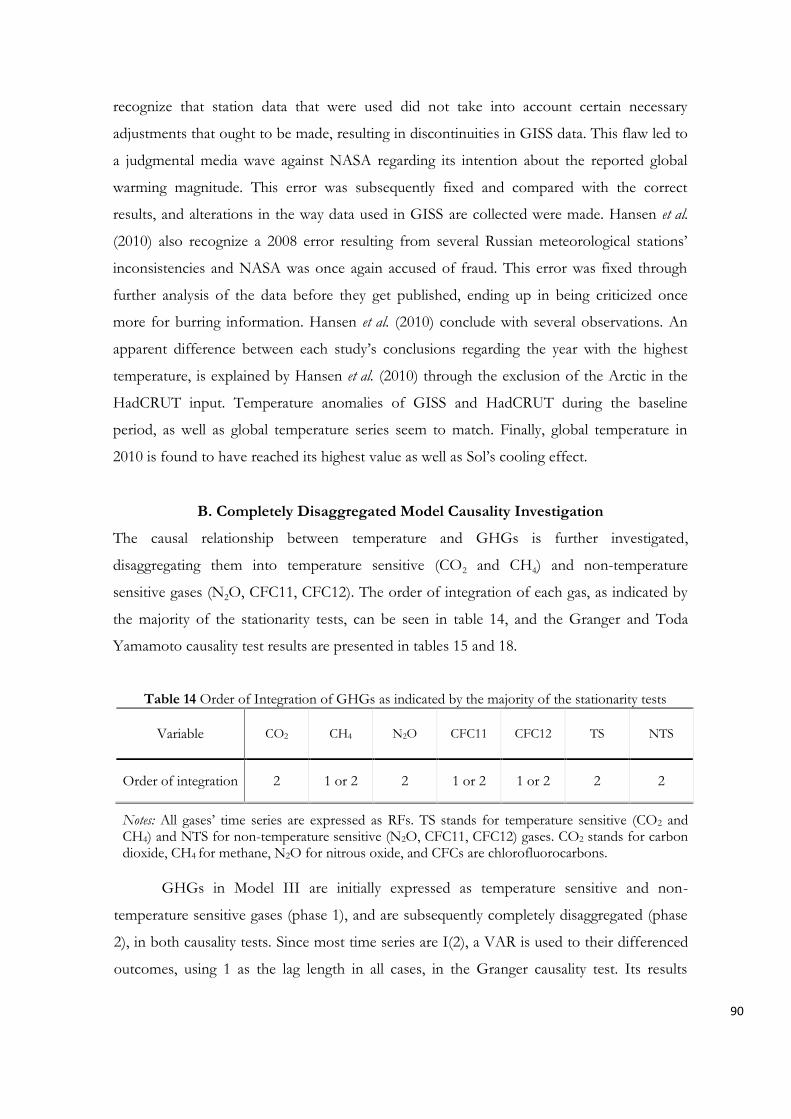
90
recognize that station data that were used did not take into account certain necessary
adjustments that ought to be made, resulting in discontinuities in GISS data. This flaw led to
a judgmental media wave against NASA regarding its intention about the reported global
warming magnitude. This error was subsequently fixed and compared with the correct
results, and alterations in the way data used in GISS are collected were made. Hansen et al.
(2010) also recognize a 2008 error resulting from several Russian meteorological stations’
inconsistencies and NASA was once again accused of fraud. This error was fixed through
further analysis of the data before they get published, ending up in being criticized once
more for burring information. Hansen et al. (2010) conclude with several observations. An
apparent difference between each study’s conclusions regarding the year with the highest
temperature, is explained by Hansen et al. (2010) through the exclusion of the Arctic in the
HadCRUT input. Temperature anomalies of GISS and HadCRUT during the baseline
period, as well as global temperature series seem to match. Finally, global temperature in
2010 is found to have reached its highest value as well as Sol’s cooling effect.
B. Completely Disaggregated Model Causality InvestigationThe causal relationship between temperature and GHGs is further investigated,
disaggregating them into temperature sensitive (CO2 and CH4) and non-temperature
sensitive gases (N2O, CFC11, CFC12). The order of integration of each gas, as indicated by
the majority of the stationarity tests, can be seen in table 14, and the Granger and Toda
Yamamoto causality test results are presented in tables 15 and 18.
Table 14 Order of Integration of GHGs as indicated by the majority of the stationarity tests
Variable CO2 CH4 N2O CFC11 CFC12 TS NTS
Order of integration 2 1 or 2 2 1 or 2 1 or 2 2 2
Notes: All gases’ time series are expressed as RFs. TS stands for temperature sensitive (CO2 andCH4) and NTS for non-temperature sensitive (N2O, CFC11, CFC12) gases. CO2 stands for carbondioxide, CH4 for methane, N2O for nitrous oxide, and CFCs are chlorofluorocarbons.
GHGs in Model III are initially expressed as temperature sensitive and non-
temperature sensitive gases (phase 1), and are subsequently completely disaggregated (phase
2), in both causality tests. Since most time series are I(2), a VAR is used to their differenced
outcomes, using 1 as the lag length in all cases, in the Granger causality test. Its results

91
indicate a two way causal relationship between both temperature time series and carbon
dioxide in all cases and methane causes temperature as well, whereas there is no such
indication as regards all the other gases. Regarding the Toda Yamamoto causality test, all
optimal lags are 1 and VAR lag lengths are 3, with the exception of the 1850 to 2011 case of
phase 2, for which optimal is 2 and VAR lag length is 4. In the full sample, temperature
sensitive gases appear to influence both temperature time series in phase 1, and only carbon
dioxide has the same effect in phase 2.
Table 15 Granger Causality Test Results of Model III with Disaggregated GHGs (VAR)
1850 – 2011(HADCRUT4)
1850 – 2011(GISSv3)
1958 – 2011(HADCRUT4)
1958 – 2011(GISSv3)
1958 – 2011(HADCRUT4)
with Ocean HeatContent
1958 – 2011(GISSv3) withOcean Heat
Content
T → TS 0.0002 0.0008 0.0001 0.0007 0.0014 0.0043TS → T 0.0003 0.0052 0.0032 0.0233 0.0471 0.1876
T → NTS 0.8702 0.4165 0.5537 0.9658 0.6328 0.8684NTS → T 0.1160 0.0427 0.2434 0.1348 0.2116 0.1061T → CO2 0.0004 0.0017 0.0001 0.0009 0.0014 0.0049CO2 → T 0.0037 0.0273 0.0267 0.1277 0.1655 0.4950T → CH4 0.1398 0.0441 0.0231 0.0417 0.0471 0.0751CH4 → T 0.1379 0.2158 0.2740 0.1855 0.2600 0.1716T → N2O 0.5260 0.3279 0.8489 0.7538 0.8303 0.7553N2O → T 0.1645 0.0873 0.2681 0.1579 0.2466 0.1355
T → CFC11 0.8100 0.5641 0.6544 0.5323 0.4075 0.3484CFC11 →T 0.8251 0.4684 0.3533 0.1510 0.3919 0.1765T → CFC12 0.3365 0.9089 0.2398 0.5055 0.4791 0.7951
CFC12 → T 0.4731 0.2012 0.6146 0.4136 0.5752 0.3648
Notes: Numbers in the table are p values. All gases’ time series are expressed as RFs. T stands fortemperature, TS for temperature sensitive (CO2 and CH4) and NTS for non-temperature sensitive(N2O, CFC11, CFC12) gases. CO2 stands for carbon dioxide, CH4 for methane, N2O for nitrous oxide,and CFCs are chlorofluorocarbons.
The Granger causality test is also performed through a VECM, for the case that a
cointegrating relationship is present and could be found. The lag lengths that were used are
presented in table 16 and results in table 17.
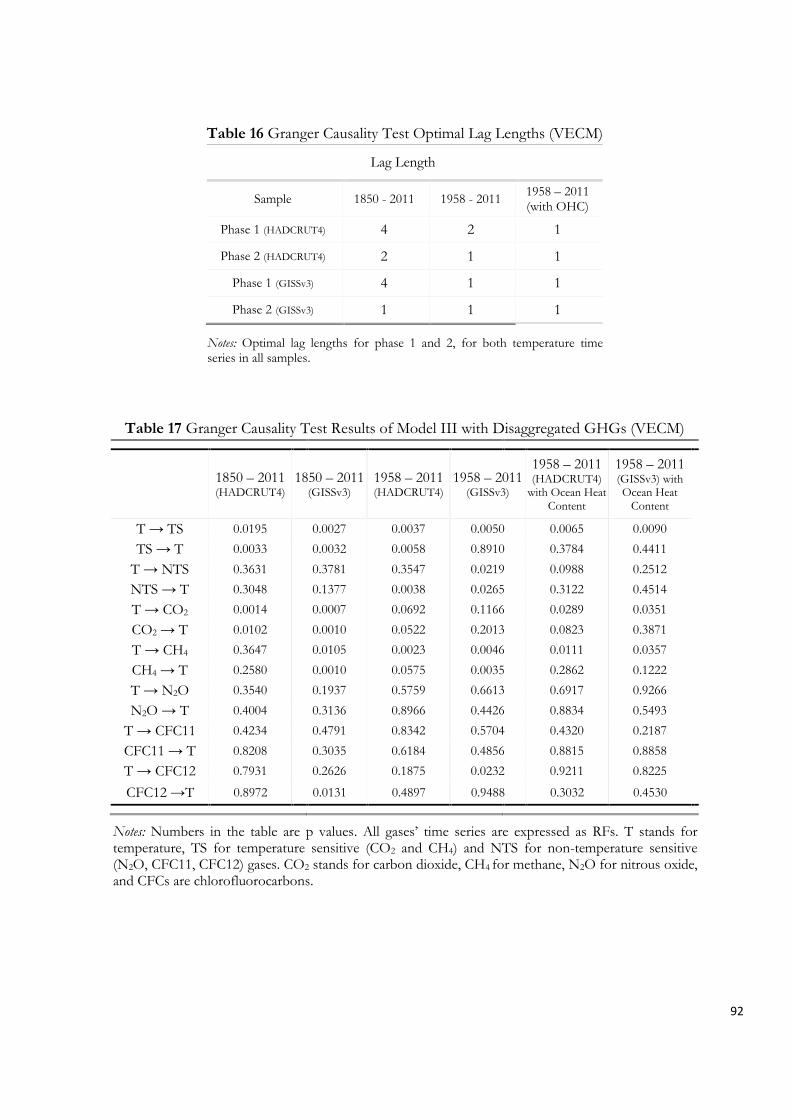
92
Table 16 Granger Causality Test Optimal Lag Lengths (VECM)
Lag Length
Sample 1850 - 2011 1958 - 2011 1958 – 2011(with OHC)
Phase 1 (HADCRUT4) 4 2 1
Phase 2 (HADCRUT4) 2 1 1
Phase 1 (GISSv3) 4 1 1
Phase 2 (GISSv3) 1 1 1
Notes: Optimal lag lengths for phase 1 and 2, for both temperature timeseries in all samples.
Table 17 Granger Causality Test Results of Model III with Disaggregated GHGs (VECM)
1850 – 2011(HADCRUT4)
1850 – 2011(GISSv3)
1958 – 2011(HADCRUT4)
1958 – 2011(GISSv3)
1958 – 2011(HADCRUT4)
with Ocean HeatContent
1958 – 2011(GISSv3) withOcean Heat
Content
T → TS 0.0195 0.0027 0.0037 0.0050 0.0065 0.0090TS → T 0.0033 0.0032 0.0058 0.8910 0.3784 0.4411
T → NTS 0.3631 0.3781 0.3547 0.0219 0.0988 0.2512NTS → T 0.3048 0.1377 0.0038 0.0265 0.3122 0.4514T → CO2 0.0014 0.0007 0.0692 0.1166 0.0289 0.0351CO2 → T 0.0102 0.0010 0.0522 0.2013 0.0823 0.3871T → CH4 0.3647 0.0105 0.0023 0.0046 0.0111 0.0357CH4 → T 0.2580 0.0010 0.0575 0.0035 0.2862 0.1222T → N2O 0.3540 0.1937 0.5759 0.6613 0.6917 0.9266N2O → T 0.4004 0.3136 0.8966 0.4426 0.8834 0.5493
T → CFC11 0.4234 0.4791 0.8342 0.5704 0.4320 0.2187CFC11 → T 0.8208 0.3035 0.6184 0.4856 0.8815 0.8858T → CFC12 0.7931 0.2626 0.1875 0.0232 0.9211 0.8225
CFC12 →T 0.8972 0.0131 0.4897 0.9488 0.3032 0.4530
Notes: Numbers in the table are p values. All gases’ time series are expressed as RFs. T stands fortemperature, TS for temperature sensitive (CO2 and CH4) and NTS for non-temperature sensitive(N2O, CFC11, CFC12) gases. CO2 stands for carbon dioxide, CH4 for methane, N2O for nitrous oxide,and CFCs are chlorofluorocarbons.

93
Table 18 Toda Yamamoto Causality Test Results of Model III with Disaggregated GHGs
1850 – 2011(HADCRUT4)
1850 – 2011(GISSv3)
1958 – 2011(HADCRUT4)
1958 – 2011(GISSv3)
1958 – 2011(HADCRUT4)
with Ocean HeatContent
1958 – 2011(GISSv3) withOcean Heat
Content
T → TS 0.0533 0.4717 0.0317 0.2002 0.0692 0.2819TS → T 0.0004 0.0008 0.0864 0.4571 0.1266 0.4721
T → NTS 0.6636 0.4340 0.2782 0.9738 0.4385 0.8739NTS → T 0.3254 0.2177 0.6263 0.4895 0.9799 0.8560T → CO2 0.0874 0.7977 0.2563 0.9667 0.3940 0.9228CO2 → T 0.0133 0.0147 0.3513 0.5954 0.5187 0.7741T → CH4 0.8312 0.8105 0.0563 0.0743 0.0995 0.0916CH4 → T 0.1538 0.1035 0.9272 0.8579 0.8200 0.8496T → N2O 0.8210 0.5146 0.6838 0.3735 0.3425 0.2646N2O → T 0.9746 0.7573 0.7951 0.5517 0.9016 0.7732
T →CFC11 0.4329 0.7267 0.5005 0.3773 0.3502 0.2659CFC11 → T 0.0871 0.2571 0.6688 0.4898 0.9390 0.9228T → CFC12 0.3378 0.6033 0.0553 0.2619 0.0720 0.2836
CFC12 → T 0.5402 0.4533 0.7515 0.9178 0.6625 0.7899
Notes: Numbers in the table are p values. All gases’ time series are expressed as RFs. T stands fortemperature, TS for temperature sensitive (CO2 and CH4) and NTS for non-temperature sensitive(N2O, CFC11, CFC12) gases. The first four causal relationships are explored through phase 1, and therest through phase 2.
For the rolling window investigation with the Toda Yamamoto causality test, optimal lag
length is 1 and VAR lag length is 3 in all cases. Results are depicted in figures 13 and 14.
a b
Figure 13 Toda Yamamoto Results (Rolling).Notes: The time period is from 1850 to 2011. The window length of Phase 1 is 100 with a step of 5. Every vertical line in the graphsrepresents the result for the 100 year window length preceding its final year. Values are the chi square outcome of each window test scaledover the 0.05 critical value of each model. The critical value used for both 13.a and 13.b figures is 3.85138. TS stands for temperaturesensitive gases and NTS for non-temperature sensitive gases. All gases’ time series are expressed as RFs.
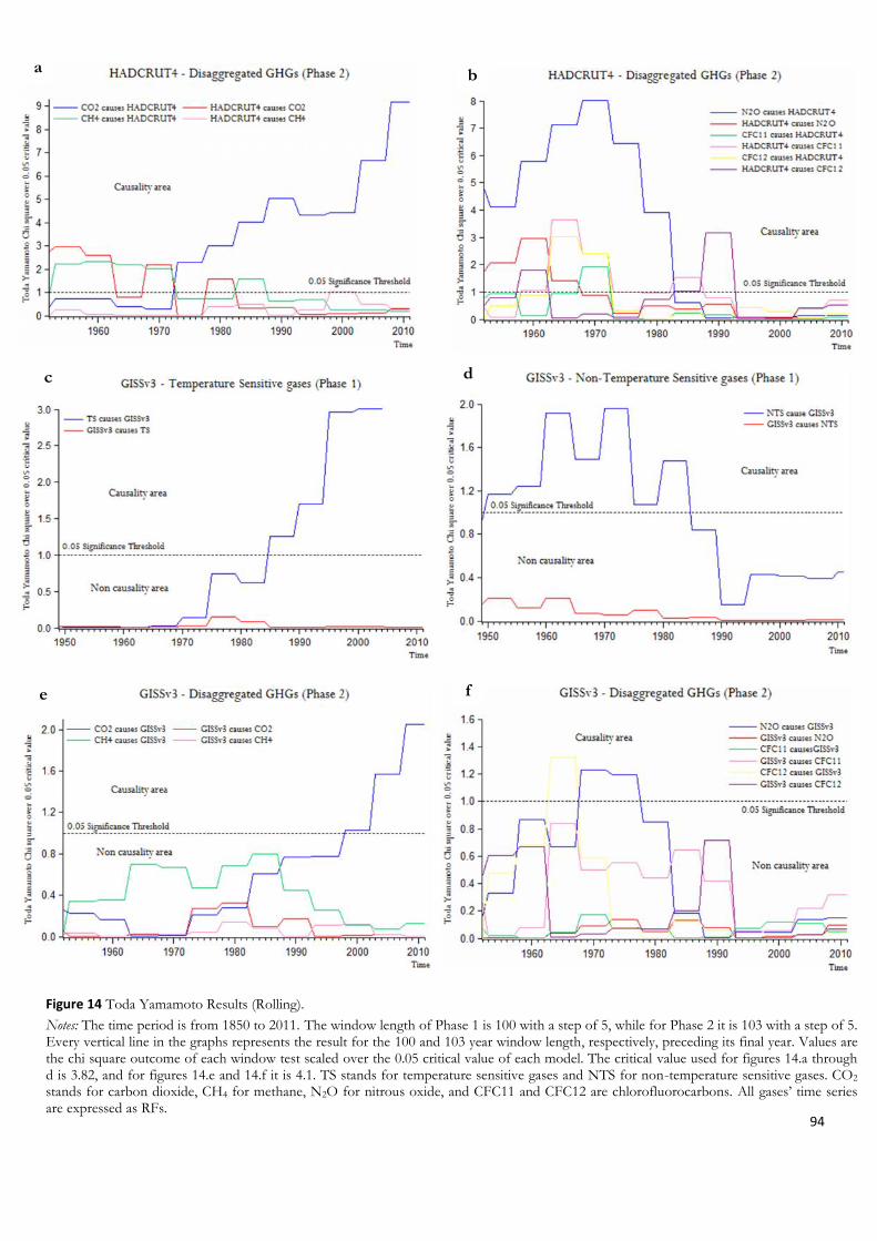
94
a b
Figure 14 Toda Yamamoto Results (Rolling).Notes: The time period is from 1850 to 2011. The window length of Phase 1 is 100 with a step of 5, while for Phase 2 it is 103 with a step of 5.Every vertical line in the graphs represents the result for the 100 and 103 year window length, respectively, preceding its final year. Values arethe chi square outcome of each window test scaled over the 0.05 critical value of each model. The critical value used for figures 14.a throughd is 3.82, and for figures 14.e and 14.f it is 4.1. TS stands for temperature sensitive gases and NTS for non-temperature sensitive gases. CO2stands for carbon dioxide, CH4 for methane, N2O for nitrous oxide, and CFC11 and CFC12 are chlorofluorocarbons. All gases’ time seriesare expressed as RFs.
c d
e f

95
C. What changes if there is cointegration in Model III and scenario 4 of Model II?
Table 19 Granger Causality Test Results – VECM
HADCRUT4Model II (scenario 4)
Sample 1850 – 2011 1958 – 2011 1958 – 2011 (with OHC)N → T 0.0234 0.0584 0.0881T → A 0.0010 0.0061 0.0353A → T 0.0581 0.0000 0.0000Sample 1850 – 2011 1958 – 2011 1958 – 2011 (with OHC)
Model IIIGHGs → T 0.0019 0.0479 0.2398
S → T 0.3133 0.3237 0.1075BC → T 0.5607 0.1595 0.2474
GHGs, S & BC → T 0.0000 0.0000 0.0000Vol → T 0.0143 0.0249 0.1547Sol → T 0.2953 0.0611 0.0146
Vol & Sol → T 0.0319 0.3506 0.9078T → GHGs 0.0039 0.2443 0.0462
GISSv3Model II (scenario 4)
Sample 1850 – 2011 1958 – 2011 1958 – 2011 (with OHC)N → T 0.0276 0.0856 0.0403T → A 0.0006 0.0358 0.0601A → T 0.0015 0.0000 0.0001Sample 1850 – 2011 1958 – 2011 1958 – 2011 (with OHC)
Model IIIGHGs → T 0.0000 0.8467 0.9274
S → T 0.0448 0.2039 0.2447BC → T 0.2413 0.2312 0.2801
GHGs, S & BC → T 0.0000 0.0000 0.0000Vol → T 0.0337 0.7606 0.4094Sol → T 0.8015 0.6860 0.7044
Vol & Sol → T 0.0703 0.1409 0.1360T → GHGs 0.0000 0.1014 0.1779
Notes: Numbers in the table are p values for each Model in the four scenarios. All gases’ time series areexpressed as RFs. BC stands for black carbon, S for anthropogenic sulfur emissions, Vol for volcanic sulfateaerosols, N for natural, T for temperature, A for anthropogenic and Sol for solar irradiance. Total representsan aggregation of natural and anthropogenic RFs, natural of Vol and Sol, and anthropogenic of GHGs (CO2,CH4, N2O and CFCs), S and BC. In Model I anthropogenic and natural RFs are aggregated and in Model IIthey are disaggregated into natural and anthropogenic. In Model III, natural are disaggregated into Vol andSol, and anthropogenic into GHGs, S and BC. Scenario 1: BC=1, S=1, scenario 2: BC=0, S=1, scenario 3:BC=3, S=1 and scenario 4: BC=0, S=0.5.

96
D. Additional Figures
Figure 16 CO2 concentration, temperature and sea level projections.Available from: http://www.ipcc.ch/ipccreports/tar/vol4/index.php?idp=42#figspm52
Figure 15 Concentrations of the main Greenhouse Gases from 0to 2005. Source: Forster et al. 2007