An Introduction to the EM AlgorithmNaala Brewer and Kehinde Salau

An Introduction to the EM AlgorithmOutline•History of the EM Algorithm
•Theory behind the EM Algorithm
•Biological Examples including derivations, coding in R, Matlab, C++
•Graphs of iterations and convergence
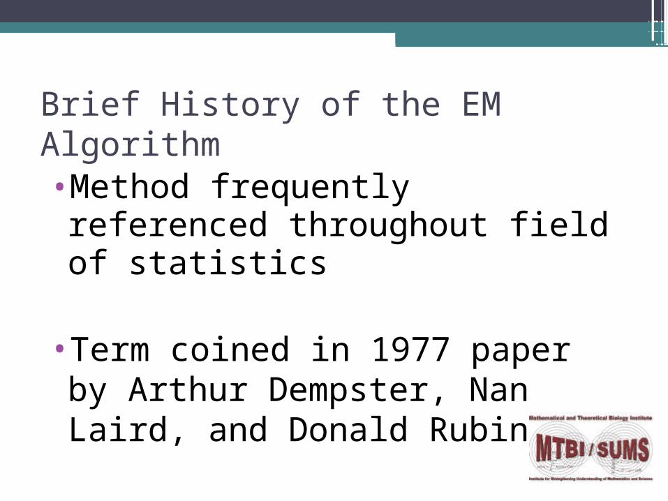
Brief History of the EM Algorithm
•Method frequently referenced throughout field of statistics
•Term coined in 1977 paper by Arthur Dempster, Nan Laird, and Donald Rubin

Breakdown of the EM Task•To compute MLEs of latent variables
and unknown parameters in probabilistic models
•E-step: computes expectation of complete/unobserved data
•M-step: computes MLEs of unknown parameters
•Repeat!!

Generalization of the EM Algorithm•X- Full sample (latent variable) ~ f(x; θ) Y - Observed sample (incomplete data) ~
f(y;θ) such that y(x) = y
•We define Q(θ;θp) = E[lnf(x;θ)|Y, θp]
•θp+1 obtained by solving, = 0

Generalization (cont.)
•Iterations continue until |θp+1 - θp| or |Q(θp+1;θp) - Q(θp;θp)| are sufficiently small
•Thus, optimal values for Q(θ;θp) and θ are obtained
•Likelihood nondecreasing with each iteration:
Q(θp+1;θp) ≥ Q(θp;θp)

Example 1 - Ecological Example•n - number of marked animals in 5
different regions, p - probability of survival
•Suppose that only the number of animals that survive in 3 of the 5 regions is known (we may not be able to see or capture all of the animals in x1, x2)
X = (?, ?, 30, 25, 39) = (x1, x2, x3, x4, x5)
•We estimate p using the EM Algorithm.

Binomial Distribution - Derivation

Binomial Derivation (cont.)
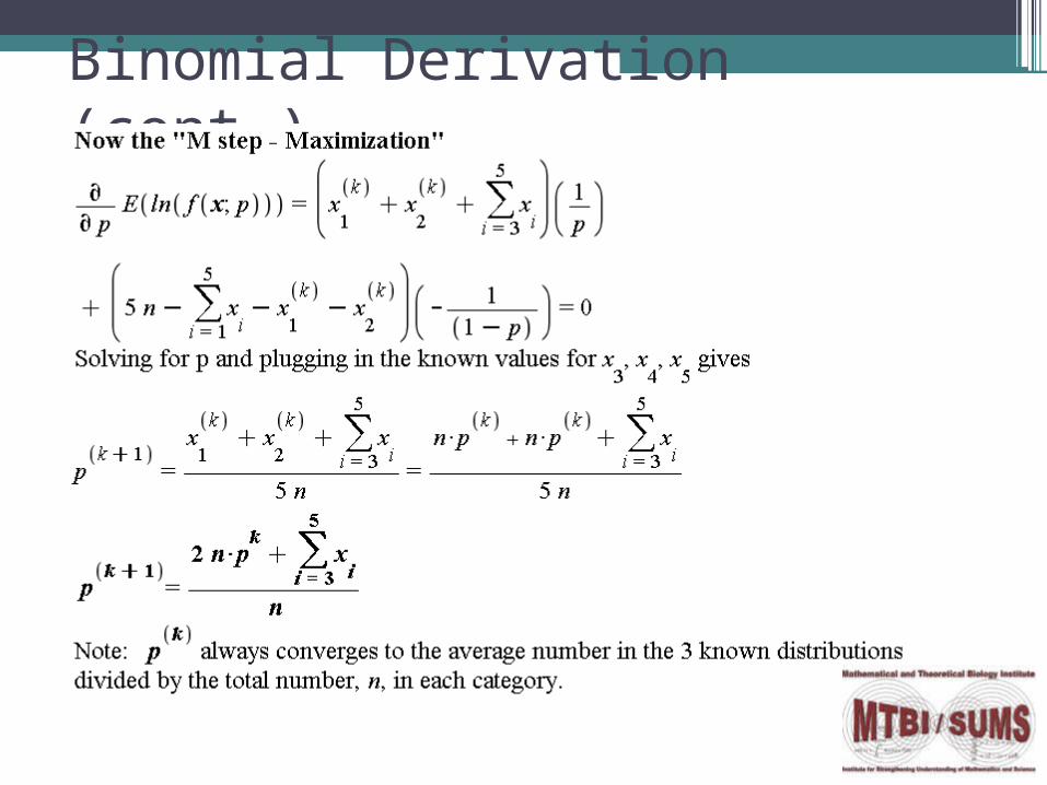
Binomial Derivation (cont.)

Binomial DistributionGraph of Convergence of Unknown
Parameter, pk
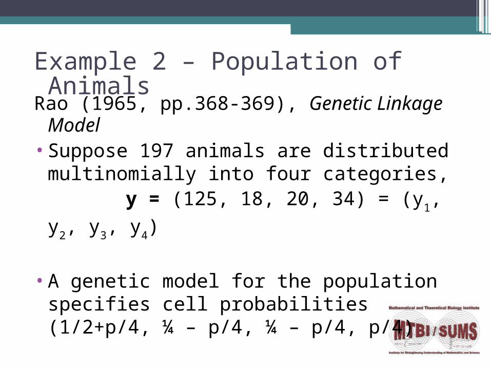
Example 2 – Population of AnimalsRao (1965, pp.368-369), Genetic Linkage Model•Suppose 197 animals are distributed multinomially
into four categories, y = (125, 18, 20, 34) = (y1, y2, y3, y4)
•A genetic model for the population specifies cell probabilities (1/2+p/4, ¼ – p/4, ¼ – p/4, p/4)
• Represent y as incomplete data, y1=x1+x2
(x1, x2unknown), y2=x3, y3=x4, y4=x5.

Multinomial Distribution-Derivation

Multinomial Derivation (cont.)

Multinomial Derivation (cont.)

Multinomial Derivation (cont.)

Multinomial Coding
Example 2 – Population of Animals•R Coding•Matlab Coding•C++ Coding
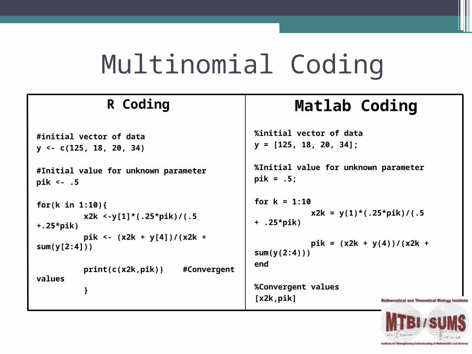
R Coding
#initial vector of data
y <- c(125, 18, 20, 34)
#Initial value for unknown parameter
pik <- .5
for(k in 1:10){
x2k <-y[1]*(.25*pik)/(.5 +.25*pik)
pik <- (x2k + y[4])/(x2k + sum(y[2:4]))
print(c(x2k,pik)) #Convergent values
}
Matlab Coding
%initial vector of data
y = [125, 18, 20, 34];
%Initial value for unknown parameter
pik = .5;
for k = 1:10
x2k = y(1)*(.25*pik)/(.5 + .25*pik)
pik = (x2k + y(4))/(x2k + sum(y(2:4)))
end
%Convergent values
[x2k,pik]
Multinomial Coding
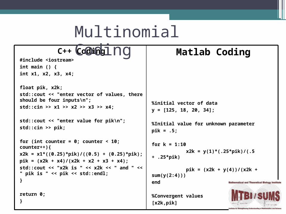
C++ Coding#include <iostream>
int main () {
int x1, x2, x3, x4;
float pik, x2k;
std::cout << "enter vector of values, there should be four inputs\n";
std::cin >> x1 >> x2 >> x3 >> x4;
std::cout << "enter value for pik\n";
std::cin >> pik;
for (int counter = 0; counter < 10; counter++){
x2k = x1*((0.25)*pik)/((0.5) + (0.25)*pik);
pik = (x2k + x4)/(x2k + x2 + x3 + x4);
std::cout << "x2k is " << x2k << " and " << " pik is " << pik << std::endl;
}
return 0;
}
Matlab Coding
%initial vector of data
y = [125, 18, 20, 34];
%Initial value for unknown parameter
pik = .5;
for k = 1:10
x2k = y(1)*(.25*pik)/(.5 + .25*pik)
pik = (x2k + y(4))/(x2k + sum(y(2:4)))
end
%Convergent values
[x2k,pik]
Multinomial Coding
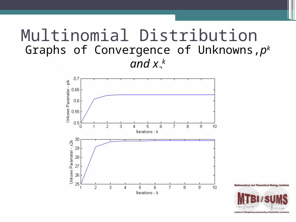
Graphs of Convergence of Unknowns,pk and x2
k
Multinomial Distribution

Example 3 -Failure TimesFlury and Zoppè (2000)▫Suppose the lifetime of bulbs follows an
exponential distribution with mean θ
▫The failure times (u1,...,un) are known for n light bulbs
▫In another experiment, m light bulbs (v1,...,vm) are tested; no individual recordings The number of bulbs, r, that fail at time t0 are recorded
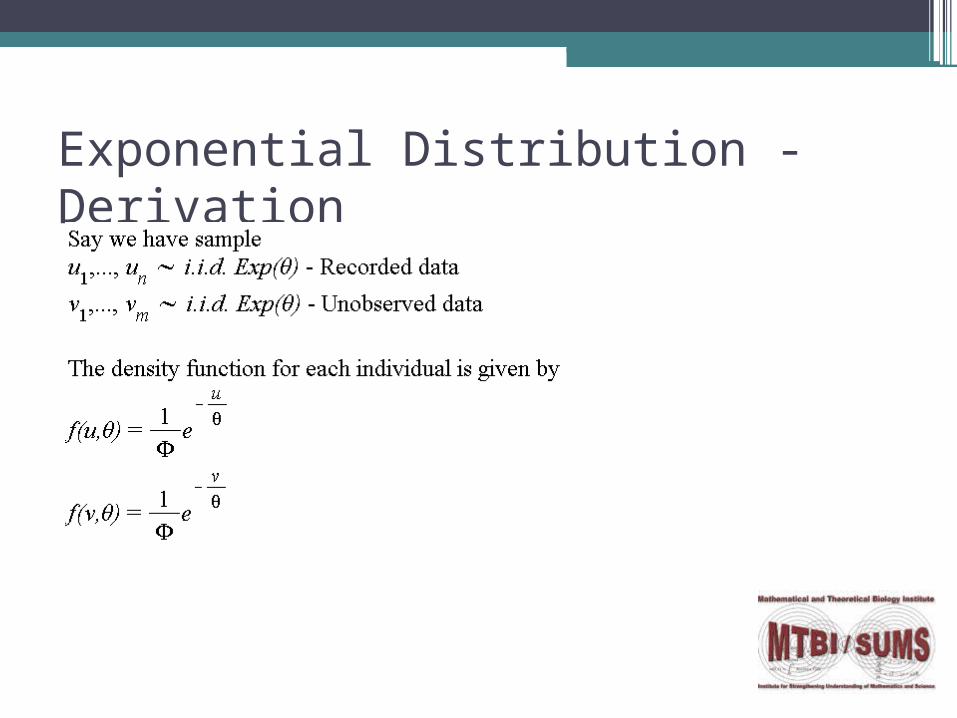
Exponential Distribution - Derivation

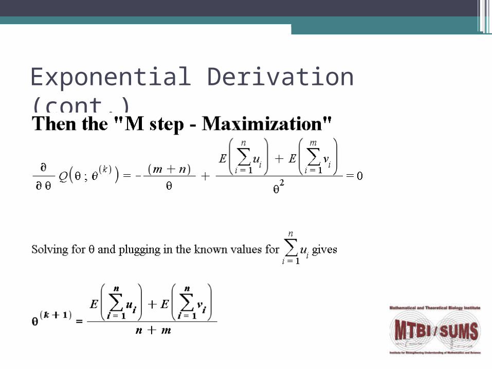
Exponential Derivation (cont.)

•Example 3 – Failure Times Graphs

Future Work
•More Elaborate Biological Examples
•Develop lognormal models with predictive capabilities for optimal interrupted HIV treatments (ref. H.T. Banks); i.e.Normal Mixture models
•Study of improved models•Monte Carlo implementation of the E step•Louis' Turbo EM

An Introduction to the EM AlgorithmReferences[1] Dempster, A.P., Laird, N.M., Rubin, D.B. (1977). Maximum
Likelihood from Incomplete Data via the EM Algorithm. Journal of the Royal Statistical Society. Series B (Methodological), Vol. 39, No. 1, , pp. 1-38
[2] Redner, R.A., Walker, H.F. (Apr., 1984). Mixture Densities, Maximum Likelihood and the EM Algorithm. SIAM Review, Vol. 26, No. 2., pp. 195-239.
[3] Tanner, A.T. (1996). Tools for Statistical Inference. Springer-Verlag New York, Inc. Third Edition

AcknowledgementsThe MTBI/SUMS Summer Research Program is supported by:
The National Science Foundation (DMS-0502349) The National Security Agency (DOD-H982300710096) The Sloan Foundation Arizona State University
Our research particularly appreciates:
Dr. Randy Eubank Dr. Carlos Castillo-Chavez