An Adaptive Probabilistic Routing
Algorithm
by
Swapnil Shukla
DEPARTMENT OF ELECTRICAL ENGINEERING
INDIAN INSTITUTE OF TECHNOLOGY, KANPUR
May 2005

An Adaptive Probabilistic Routing
Algorithm
A Thesis Submitted
in Partial Fulfillment of the Requirements
for the Degree of
Master of Technology
by
Swapnil Shukla
to the
DEPARTMENT OF ELECTRICAL ENGINEERING
INDIAN INSTITUTE OF TECHNOLOGY, KANPUR
May 2005
ii
CERTIFICATE
It is certified that the work contained in the thesis entitled “An Adaptive Probabilis-
tic Routing Algorithm ” by Swapnil Shukla has been carried out under my supervision
and that this work has not been submitted elsewhere for a degree.
(Dr. Y. N. Singh)
May 2005 Associate Professor,
Department of Electrical Engineering,
Indian Institute of Technology,
Kanpur-208016.

iii
Acknowledgments
This thesis is dedicated to my parents,my uncle and my sister.
I express my deep sense of gratitude toward my thesis supervisor Dr. Y. N. Sign
for his invaluable guidance, moral support and constant encouragement, which helped
me to survive through the crests and troughs of my thesis work. It is my pleasure to
give my appreciation to him for taking so much interest in my academic and personal
welfare
I would like to thank my friends specially Aaksh, Amit, Bhaumik, Deepak, Navin,
Prabodh, Rajiv and Prasanna for making my stay at IIT Kanpur a memorable one.
Swapnil Shukla

iv
Abstract
The internet has grown and changed ever since the first connections were made in
1969. The problem of routing assignments has been one of the most intensively studied
areas in the fields of data networks since then. Network routing essentially consists of
two entities the Routing Protocol and the Routing Algorithm. The routing protocol
provides each node in a network, a consistent view of the topology and the routing
algorithm provides the intelligence to compute paths between nodes.The focus of this
thesis is on Routing Algorithm.
Routing algorithms can broadly be classified into Selfish and Non-Selfish Routing
Algorithms. This thesis starts with discussion of the problems faced with Selfish routing
algorithms and presents a Non-Selfish Routing Algorithm with the aim to solve the
problems. This algorithm falls into category of multipath routing. Performance of the
network is improved because the resources of multiple paths are utilized.
Finally extensive simulations have been carried out for evaluation of the perfor-
mance of the algorithm in different scenarios. The factors that decide the performance
of a network are how frequently updates are sent and how frequently routes are com-
puted. The effect of variation of these factors on convergence time, load on routers
and the queue size have been studied.

Contents
1 Introduction 1
1.1 Routing in the Internet . . . . . . . . . . . . . . . . . . . . . . . . . . . 2
1.1.1 Subnetting . . . . . . . . . . . . . . . . . . . . . . . . . . . . . . 4
1.1.2 Hierarchical Routing . . . . . . . . . . . . . . . . . . . . . . . . 5
1.2 Goals of Routing Protocols . . . . . . . . . . . . . . . . . . . . . . . . . 6
1.3 Existing Routing Algorithms . . . . . . . . . . . . . . . . . . . . . . . . 8
1.3.1 The Distance Vector Routing Algorithm . . . . . . . . . . . . . 8
1.3.2 The Link State Routing Algorithm . . . . . . . . . . . . . . . . 9
1.4 Problems with Selfish Routing . . . . . . . . . . . . . . . . . . . . . . 10
1.5 Work Done . . . . . . . . . . . . . . . . . . . . . . . . . . . . . . . . . 11
1.6 Organization of the thesis . . . . . . . . . . . . . . . . . . . . . . . . . 11
2 The Probabilistic Routing Algorithm 13
2.1 Structure of the Routing Table . . . . . . . . . . . . . . . . . . . . . . 13
2.2 Advantages of the Structure . . . . . . . . . . . . . . . . . . . . . . . . 14
2.2.1 Using Multiple Paths . . . . . . . . . . . . . . . . . . . . . . . . 14
v
vi
2.2.2 Network Oscillations . . . . . . . . . . . . . . . . . . . . . . . . 14
2.2.3 Routing Loops . . . . . . . . . . . . . . . . . . . . . . . . . . . 15
2.3 The Algorithm . . . . . . . . . . . . . . . . . . . . . . . . . . . . . . . 17
2.3.1 Computation of the Routing Table . . . . . . . . . . . . . . . . 17
2.4 Example Network . . . . . . . . . . . . . . . . . . . . . . . . . . . . . . 22
3 Simulation and Results 30
3.1 Implementation Details . . . . . . . . . . . . . . . . . . . . . . . . . . . 30
3.2 Factors affecting the performance . . . . . . . . . . . . . . . . . . . . . 33
3.3 Results . . . . . . . . . . . . . . . . . . . . . . . . . . . . . . . . . . . . 35
3.3.1 Convergence Time . . . . . . . . . . . . . . . . . . . . . . . . . 35
3.3.2 Load on the Routers . . . . . . . . . . . . . . . . . . . . . . . . 39
3.3.3 Size of the Queue . . . . . . . . . . . . . . . . . . . . . . . . . . 40
4 Conclusion 42
4.1 Future Aspects . . . . . . . . . . . . . . . . . . . . . . . . . . . . . . . 43

List of Figures
2.1 Scenario depicting Network Oscillations . . . . . . . . . . . . . . . . . . 15
2.2 Scenario demonstrating Network Loop . . . . . . . . . . . . . . . . . . 16
2.3 Demonstration of update rejection . . . . . . . . . . . . . . . . . . . . . 21
2.4 Example Network . . . . . . . . . . . . . . . . . . . . . . . . . . . . . . 22
3.1 Network A . . . . . . . . . . . . . . . . . . . . . . . . . . . . . . . . . . 32
3.2 Network B . . . . . . . . . . . . . . . . . . . . . . . . . . . . . . . . . . 33
3.3 Convergence Time vs Route Computation Delay for Network A . . . . 36
3.4 Convergence Time vs Route Computation Delay for Network B . . . . 37
3.5 Convergence Time vs Number of Events for Network A . . . . . . . . . 37
3.6 Convergence Time vs Number of Events for Network B . . . . . . . . . 38
3.7 Router Load in percentage vs Route Computation Delay for Network A 39
3.8 Router load in percentage vs Route Computation Delay for Network B 40
3.9 Size of Queue on a router vs Time . . . . . . . . . . . . . . . . . . . . . 41
vii
Chapter 1
Introduction
Computer networks have been growing at an enormous rate ever since the concept
was first proposed, for example, networks were first designed with two different pur-
poses which later on merged to form the internet. The military network (MILNET)
was designed to keep military communications working under a war. The American
University Networks (National Science Foundation Network, NSFNET / Advanced Re-
search Projects Agency Network, ARPANET) were designed to make the exchange of
research results easier.
Large-scale, wide area data networks are a part of todays global communication
infrastructure. Networks such as the Internet have become an integral medium of
information transfer, ranging from personal communication to electronic commerce
and entertainment. The importance of such networks will keep on increasing as the
electronic world becomes more and more prevalent.
The basic function of a data network is very simple: delivering data from one
1

2
network node to another. Data networks can be viewed as huge graph with routers
as vertices and transmission lines as edges. On such a huge graph the data packets
must find their way from the source to the destination. Routing can be described as
the process of creating a logical connection between nodes in a network so that packets
sent by a node can reach their destination [13].
The challenge in developing network routing algorithms is in dealing with the scale
and distribution of the physical network. As wide area networks have nodes on the
order of tens of thousands, routing algorithms must be scalable. Moreover, routing
algorithms must be able to calculate paths in a distributed manner due to the global
and distributive nature of physical networks. Also, routing algorithms need to cope
with events such as node and link failures and recalculate paths whenever such events
occur. Finally, routing algorithms need to calculate paths to allow nodes to achieve
high network performance.
1.1 Routing in the Internet
The Internet is a global data network having millions of hosts. The Internet is a best
effort datagram network: units of data transmission are packetized, and each packet is
individually and independently delivered (hop-by-hop) to its destination without any
guarantee of success, packets can be dropped in transit [9]. In order for a node to
send packets to another node, the sending node must specify the destination node.
In the Internet today, every node is uniquely identified by an 32 bit IP address [12].
3
Thus for node A to send a packet to node B, A must designate the IP address of B as
the packet’s destination. This universal naming allows every node in the Internet to
uniquely identify every other node.
Physically, the Internet is a collection of smaller inter-networks called routing do-
mains (or autonomous systems). Each routing domain is responsible for routing packets
within itself. That is, packets destined to hosts in a routing domain are routed by the
domain’s routing algorithm. An intra-domain routing algorithm refers to a routing
algorithm that routes packets within a domain, and an inter-domain routing algorithm
is responsible for routing packets between domains. Using this organization, packets
sent from one domain to another are first routed out of the sending domain, then to
the destination domain, and finally to the destination host by the destination domain’s
routing algorithm. Thus, logical Internet connectivity is ensured by the cooperation of
inter- and intra-domain routing algorithms.
It is practically impossible to maintain an entry for every destination (host) in the
internet, because of two reasons. Firstly the size of routing table will be enormous
this will require a large amount of space on the routers. Secondly the time taken to
look up a destination in such an enormous table will be very high. Because of the
size of the Internet, two methods are used to make the network scalable: subnetting
and hierarchical routing domains. Subnetting uses the IP addressing structure so
that routers can route packets based on a set of hosts instead of individual hosts, and
hierarchical routing domains reduce the size of routing domains. Both of these methods
4
are described below.
1.1.1 Subnetting
Internet addresses are divided into subnets. A subnet is identified by its IP address
prefix. Whenever an organization wants to connect to the Internet, it needs to obtain
a unique subnet address or a set of unique subnet addresses. Furthermore, every host
owned by the organization that connects to the Internet needs to have an IP address
such that the IP prefix of the host address is the same as one of the subnet addresses
obtained by the organization. The number of bits in the IP prefix is variable length.
With subnet addressing, routers outside a subnet need to know and maintain only
a single route (i.e. state) for all the hosts in the subnet. That is, routers outside a
particular subnet do not need to maintain a route for every hosts in that subnet, but
rather, these routers only need to maintain one route to the subnet; this route is used
to forward packets to every host in that subnet. Because several thousand hosts can
have the same subnet address, subnetting allows substantial space savings in routers,
making routing over the Internet more scalable.
However, subnetting alone is not enough to provide scalability because there are
hundreds of thousands of subnet addresses in the Internet. To further reduce the
amount of information that routers have to process and store, hierarchical routing
domains are used.
5
1.1.2 Hierarchical Routing
Hierarchical routing allows a routing domain to contain subnet addresses as well as
other routing domains (represented by a set of subnet addresses). Conceptually, routing
is hierarchically structured such that at the lowest level, a routing algorithm routes
packets to hosts with the same subnet address. At the second level, a routing algorithm
routes packets among second-level routing domains using the subnet addresses the
routing domains encompass. Similarly, at level i, a routing algorithm routes packets
to the appropriate level i routing domain that contains the packets destination subnet
address.
Because of the inclusive property of routing domains, a packet is routed to level i+1
if the packet is destined for a subnet address that is not in level i. Eventually, routers
in the highest level of the hierarchy, say level L, know about every subnet address and
the level L routing domain that contains the address.
Thus a packet destined for a different subnet first travels up the domain hierarchy,
until it reaches the routing domain that is the first common ancestor of both the source
and destination routing domains. From this ancestor domain, the packet then travels
down the hierarchy until it reaches the destination domain. The destination domain’s
routing algorithm then ensures the packet reaches its destination.
This hierarchical organization achieves scalability because a routing algorithm op-
erating in a level i routing domain only needs to compute paths to nodes at that level.
A node at level i could be a host (if i = 1) or a level i− 1 routing domain. If a node is

6
a routing domain, then the node advertises the subnet addresses that it encompasses.
With this hierarchical structure, a routing algorithm at a particular level only has to
compute paths to nodes at that level, thereby reducing the size of path recomputations
that routers need to perform.
Conceptually, the Internet routing hierarchy can have many levels. However, in
practice, the Internet routing is divided into only two levels, intra-domain (lower level)
and inter-domain (higher level) routing levels. Although the size of host addresses is
different from domain addresses, a routers basic mechanisms for computing paths and
forwarding packets are the same. Thus, the routing algorithm described in this thesis
are applicable for all the levels of the routing hierarchy.
1.2 Goals of Routing Protocols
A lot of Routing protocols [3, 5, 8] have been developed for this purpose they all vary
in the way they accomplish the task, but they all have more or less common goals.
The main goals are [4, 6]:
• Low latency for end to end communication. Latency is the time taken by the
packet to reach its destination from its source.
• Low latency jitter for end to end communication. Latency jitter is the variation
in latency, for real time applications such as streaming video, the requirement for
low latency jitter is more important than the requirement of low latency.

7
• High throughput for end to end communication. Throughput can be defined
as the number of data packets delivered per second. Throughput is affected by
packets being dropped, and protocol data units that are used by protocols to set
up communication with peers.
• Low packet loss or High Reliability. Packet loss causes decrease in throughput
and increases latency.
• Low convergence time in case of changes in network topology. It is necessary for
routing algorithm to adapt to changes in network as quickly as possible, so that
utilization of network resources is maximized.
• Low routing overhead. Routing overhead is caused by the update packets that
are exchanged by routing protocols to convey network information to its peers.
Routing overhead decreases throughput.
It is not possible for a routing protocol to achieve all the goals. As some of the
above stated goals are conflicting in nature, for example to achieve Low convergence
time in case of change in topology certainly requires high routing overhead which in
turn reduces the throughput for end to end communication.
Normally routing is split into two groups: Source Routing and Destination Routing.
Source Routing is where the source specifies the path a packet should traverse to
reach its destination. This requires each node in the network to have a precise

8
knowledge of the network, which seems almost impossible to accomplish on the
networks which are dynamic in nature and hence hampers the adaptiveness.
Destination Routing is where each node knows in which direction to forward a
packet for a given destination. Here the source node has no control over the path
a packet traverses. The internet works on this kind of routing.
In dynamically changing networks Source Routing is not deployed and Destination
Routing is the obvious choice.
1.3 Existing Routing Algorithms
The chapter begins by describing the two predominant routing algorithms, the Distance
Vector and Link State routing algorithms [14, 26], which are the basis of many Internet
routing protocols. This section briefly summarizes the two algorithms.
1.3.1 The Distance Vector Routing Algorithm
The distance vector [7] routing algorithm is a distributed, adaptive routing algorithm
that computes shortest paths between all node pairs. The distance vector routing
algorithm is the basis of many practical routing algorithms currently in use.
Here a router computes a routing table which is used to forward packets on the
best known path to its destination. Each entry in a routing table contains three
elements: the destination address, the next-hop neighbor on the known shortest path
to that destination, and the cost of the known path. Each routers forwarding table is

9
continually updated by the distributed Distance Vector algorithm to indicate, via the
next-hop entry, the shortest path between nodes. Routers update their routing tables
by exchanging path information with their neighbors via distance vector packets. A
distance vector packet carries the identity of the originating router and a list of distance
vectors of the form (dst addr, cost), which are taken from the routers forwarding table.
Routers exchange distance vector packets with their neighbors periodically or in
response to link/node failures or recoveries. After distance vector routing tables con-
verge, routers will then forward packets to their destinations on the calculated shortest
paths. Because distance vector routing computes all pairs single shortest paths, tag-
ging a packet with its destination address uniquely identifies the packets path through
the network. To send a packet to the destination the router looks up the entry in its
routing table for the destination and forwards the packet to the next-hop listed in table
entry.
1.3.2 The Link State Routing Algorithm
The Link State algorithm is another routing algorithm on which many protocols are
based. In the LS routing algorithm, every router periodically broadcasts (via flooding)
its local connectivity. This information is flooded in a Link State packet (LSP) which
consists of the routers ID, a list of its neighbors IDs, and the cost of each connecting
link. After all routers broadcast their LSP, every router knows the entire network
topology. A router then computes a shortest-path spanning tree keeping itself as the
10
root of that tree. This information is then encoded in the routing table. A Link State
routing table comprises of a list of tuples of the form (dst addr, next-hop), where dst
addr is the address of the destination, and next-hop is the neighboring router on the
shortest path to that destination.
The method of sending a packet in Link State routing is exactly the same as that
for distance vector routing
1.4 Problems with Selfish Routing
The biggest problem with selfish routing [17, 18] is that the routing decision is based
node’s perspective rather than on a system-wide perspective this leads to suboptimal
system behavior. Some research has been done to find out the effect of selfish routing on
network’s efficiency [15, 16, 19] and how much selfish routing hampers the performance
of network [20, 21, 22].
Selfish routing has three major drawbacks [23].
1. Only one path per source-destination pair is used, while other paths are left
unused, this potentially limits the throughput of the network.
2. It is susceptive to oscillation, these oscillations are caused due to abrupt shift in
traffic from one link to another when some of the shortest paths change because
of change in link lengths.
3. If a routing loop exists the data packet will keep on traversing in the loop till

11
routing table is again updated.
1.5 Work Done
This thesis presents probabilistic adaptive routing algorithm. This algorithm is pro-
posed as a solution to the problems faced by selfish routing. As opposed to selfish
routing which decides in favor of single path, it assigns probabilities multiple paths be-
tween a source destination. This improves the utilization of available network resources
mainly the bandwidth. Simulations of the algorithm were carried out to measure the
performance of the algorithm in dynamic networks.
1.6 Organization of the thesis
Chapter 1 gives the basic background of routing in todays internet. Then it discusses
the basic goals of routing in communication networks. After that a brief introduction
of the link state and distance vector routing is presented. These two algorithms form
the base of most of the routing protocols currently employed in the internet. Then the
problems faced with Selfish Routing are described.
Chapter 2 describes the probabilistic routing algorithm and the structure of the
routing table. Then it gives a description of how the problems are solved. Finally this
chapter concludes with an example of working of this algorithm on a simple network.
Chapter 3 describes the implementation and simulations carried out to study the
performance of the probabilistic routing algorithm, and presents the results obtained

12
from the simulations.
Chapter 4 gives the conclusion and scope for future work.

Chapter 2
The Probabilistic Routing
Algorithm
This chapter presents a Probabilistic Routing Algorithm as a solution to the problems
stated in the previous chapter.
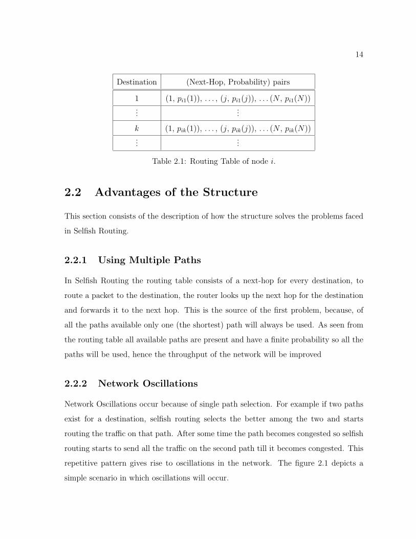
2.1 Structure of the Routing Table
The Routing Table for the algorithm consists of the pairs of next-hop and the prob-
ability of data packet taking that path. Consider a node i in the network having N
neighbors. The routing table of node i, for every destination k will have probabilities
pik(j) for every neighbor j ∈ 1, . . . , N . The routing table of node i is shown in Table
2.1
where the entity pik(j) stands for probability of path from node i to destination
node k via neighbor j. All probabilities satisfy:
pik(j) ≥ 0
and, ∑j
pik(j) = 1
13
14
Destination (Next-Hop, Probability) pairs
1 (1, pi1(1)), . . . , (j, pi1(j)), . . . (N , pi1(N))...
...
k (1, pik(1)), . . . , (j, pik(j)), . . . (N , pik(N))...
...
Table 2.1: Routing Table of node i.
2.2 Advantages of the Structure
This section consists of the description of how the structure solves the problems faced
in Selfish Routing.
2.2.1 Using Multiple Paths
In Selfish Routing the routing table consists of a next-hop for every destination, to
route a packet to the destination, the router looks up the next hop for the destination
and forwards it to the next hop. This is the source of the first problem, because, of
all the paths available only one (the shortest) path will always be used. As seen from
the routing table all available paths are present and have a finite probability so all the
paths will be used, hence the throughput of the network will be improved
2.2.2 Network Oscillations
Network Oscillations occur because of single path selection. For example if two paths
exist for a destination, selfish routing selects the better among the two and starts
routing the traffic on that path. After some time the path becomes congested so selfish
routing starts to send all the traffic on the second path till it becomes congested. This
repetitive pattern gives rise to oscillations in the network. The figure 2.1 depicts a
simple scenario in which oscillations will occur.

15
Figure 2.1: Scenario depicting Network Oscillations
To route the traffic from node A to node E will selfish routing will choose one route
ABDE (say). Once the path becomes congested it will start to route packets on the
path ACDE till it becomes congested, and the pattern repeats itself.
For the same scenario probabilistic routing will route packets on both routes hence
none of the routes will be congested.
2.2.3 Routing Loops
Figure 2.2 depicts a scenario in which routing loop can occur. In case of Selfish Routing
if for sending a packet from node A to node G. The routing tables of the nodes B,
C and D in the network are as shown in the table below. Node A will send packets
to either node B or node C. If packets are sent to B then the path traversed will be
ABDCBD and if the packets are sent to C then the path traversed will be ACBDCB
and a routing loop will occur in both cases.
While in case of Probabilistic Routing there will be finite probabilities of packets
taking any given path. The probability that a packet will be stuck in a loop is low.

16
Furthermore, even if a packet traverses a loop, it will not stay in the loop till the
routing table is updates.
Figure 2.2: Scenario demonstrating Network Loop
Dest. NextHop Dest. NextHop Dest. NextHop
A A A A A C
B B B B B B
C C C C C C
D D D D D D
E C E E E C
F F F D F F
G D G B G C

17
2.3 The Algorithm
This section presents the routing algorithm developed to create the routing table shown
in Section 2.1. The goal is to assign probabilities to paths via each neighbor according
to the cost to the destination.
Consider a node i with N neighbors. For computing the routing table at node i for
destination k. The node i has to store the following:
• qik(j) It is the probabilistic weight for a path from node i to node k via neighbor
j. This weight is proportional to the cost of the path from node i to node k via
neighbor j.
• qprevik (j) It is the previous value of qik(j).
• pik(j) It is the probability of choosing the path from node i to node k via neighbor
j. All probabilities satisfy pik(j) ≥ 0 and∑
j pik(j) = 1.
• pprevik (j) It is the previous value of pik(j).
• lj It is the cost from the node i to its neighbor j.
• Ljk It is the estimated cost to the destination k as reported by neighbor j.
2.3.1 Computation of the Routing Table
This section describes how the routing table at node i for the destination k is computed.
After receiving an update Ljk from neighbor j, node i updates its cost estimate
Lik(j) i.e. estimated cost to destination k via neighbor j using equation 2.1. This
procedure is repeated for every neighbor.
Lik(j) = lj + Ljk (2.1)
Node i then computes overall cost estimate to destination k using equation 2.2.
This overall cost estimate is used for assigning probabilistic weights to each path and
18
is sent as an update to every neighbor of node i.
E[Lik] =∑j
pprevik (j)Lik(j) (2.2)
Initially when routing table does not exists the algorithm uses equal probabilities
for computing the estimated cost. The equal probabilities are only for paths through
those neighbors from which update for the destination is received. All the following
computations use previous values of probabilities.
Using the estimated costs node i then computes the probabilistic weights for each
path using equation 2.3.
qik(j) = qprevik (j) +
qprevik (j)(E[Lik]− Lik(j))
ω(2.3)
Initially when the routing table does not exists all qprevik (j) are assigned equal weights
1. For all further computations previous values of qik(j) are used. ω is a weighing factor
used to deal with negative values of E[Lik]− Lik(j).
If the cost of path to destination k via neighbor j satisfies
Lik(j) < E[Lik]
i.e. the path through neighbor j has less cost than the estimated cost then
qik(j) > qprevik (j)
the probabilistic weight of the path through neighbor j increases. If the cost of path
to destination k via neighbor j satisfies
Lik(j) > E[Lik]
i.e. the path through neighbor j has more cost than the estimated cost then
qik(j) < qprevik (j)
the probabilistic weight of the path through neighbor j decreases. This ensures that
paths with low cost have high probabilistic weights and paths with high cost will have
low probabilistic weights.
19
As the desired relationship between cost of the paths and probabilistic weights has
been established node i uses equation 2.4 to compute the probabilities.
pik(j) =qik(j)∑j qik(j)
(2.4)
Node i uses the values of pik(j) to update the routing table. The algorithm is
explained below:

20
Do forever
[
If an event occurs
[
For every neighbor j ∈ 1 . . . N
[
assign all qik(j) to qprevik (j)
assign all pik(j) to pprevik (j)
compute Lik(j) using equation 2.1
compute E[Lik] using equation 2.2
compute qik(j) using equation 2.3
compute pik(j) using equation 2.4
update the routing table
]
For every destination in the routing table
[
Send an update to every neighbor
]
]
]
An event is either an arrival of update or a link going up or down, or a link’s cost
changes.
A node will not send the update for a destination to the neighbors through which
it has the path to that destination. Consider a node S having 5 neighboring nodes A,
B, C, D and E . If for target node T , node S has paths through neighbors A, B and E ,
then S will send the update LST only to nodes C and D. The update LST will not be
sent to A, B and C.
Also, when an update Ljk is received at node i, if the destination k is also neighbor

21
of node i, then it is checked whether neighbor j is reporting a path with less cost than
the direct path to neighbor k. If neighbor j reports a path with lesser cost then the
update Ljk is used for computing the routing table otherwise the update is rejected.
This scenario is depicted in figure 2.3.
When node E receives an update LCD (of cost 5) it calculates LED(C) = lC + LCD
and compares it with lD. In this case LED(C) < lD so the update is not used in
computation.
When node C receives an update LED (of cost 2) it calculates LCD(E) = lE + LED
and compares it with lD. In this case LCD(E) > lD so node C uses this node in
computation of routing table.
Figure 2.3: Demonstration of update rejection

22
2.4 Example Network
Figure 2.4 shows a simple network which will be used to show how the routing algorithm
works.
Initially node 1 has information only about its neighbors (2, 3 and 4) so it creates
an entry for each of its neighbors. The routing table of node 1 looks like:
Dest. (NextHop, Probability)
2 (2, 1)
3 (3, 1)
4 (4, 1)
Figure 2.4: Example Network
Similarly the initial routing tables of nodes 2, . . . , 5 contain only information about
their respective neighbors. Their routing tables have similar form as node 1.
Node 2 sends an update L25, similarly node 3 sends two updates L34 and L35, and
node 4 sends two updates L43 and L45 to node 1. Consider update L34, node 1 has the

23
direct path to node 4, l4 = 7, using equation 2.1 node 1 computes:
L14(3) = l3 + L34 = 4 + 5 = 9
which is more than l4 hence this update is rejected. Similarly using equation 2.1 node
1 computes:
L13(4) = l4 + L43 = 7 + 5 = 12
hence the update L43 is also rejected because l3 < L13(4).
There are three updates for node 5, L25 = 6, L35 = 2 and L45 = 2. Now l2 = 3,
l3 = 4 and l4 = 7. Substituting these values in equation 2.1 node 1 computes:
L15(2) = l2 + L25 = 3 + 6 = 9
L15(3) = l3 + L35 = 4 + 2 = 6
and
L15(4) = l4 + L45 = 7 + 2 = 9
As there is no entry for node 5 the previous values of probabilistic weights are qprev15 (2) =
qprev15 (3) = qprev
15 (4) = 1, similarly the previous values of routing probabilities are
pprev15 (2) = pprev
15 (3) = pprev15 (4) = 1/3.
These values are substituted in equation 2.2 and estimated cost to node 5 comes
out to be
E[L15] =1
3[9 + 6 + 9] = 8
Using equation 2.3 the probabilistic weights become q15(2) = 0.9, q15(3) = 1.2 and
q15(4) = 0.9. Using equation 2.4 the probabilities are computed and we get p15(2) = 0.3,
p15(3) = 0.4 and p15(4) = 0.3. The routing table of node 1 becomes:
Dest (NextHop, Probability)
2 (2, 1)
3 (3, 1)
4 (4, 1)
5 (2, 0.3), (3, 0.4), (4, 0.3)
24
Node 2 receives updates L13 = 4 and L14 = 7 from node 1 and updates L53 = 2
and L54 = 2. Consider updates L13 = 4 and L53 = 2 first, node 2 already has l1 = 3
and l5 = 6. Substituting these values in equation 2.1 node 2 computes
L23(1) = l1 + L13 = 3 + 4 = 7
L23(5) = l5 + L53 = 6 + 2 = 8
As there is no entry for node 3 the previous values of probabilistic weights are qprev23 (1) =
qprev23 (5) = 1, similarly the previous values of routing probabilities are pprev
23 (1) =
pprev23 (5) = 1/2.
These values are substituted in equation 2.2 and estimated cost to node 3 comes
out to be
E[L23] =1
2[7 + 8] = 7.5
Using equation 2.3 the probabilistic weights become q23(1) = 1.05 and q23(5) = 0.95.
Using equation 2.4 the probabilities are computed and we get p23(1) = 0.525 and
p23(5) = 0.475.
Consider updates L14 = 7 and L54 = 2 first, node 2 already has l1 = 3 and l5 = 6.
Substituting these values in equation 2.1 node 2 computes
L24(1) = l1 + L14 = 3 + 7 = 10
L24(5) = l5 + L54 = 6 + 2 = 8
As there is no entry for node 4 the previous values of probabilistic weights are qprev24 (1) =
qprev24 (5) = 1, similarly the previous values of routing probabilities are pprev
24 (1) =
pprev24 (5) = 1/2.
These values are substituted in equation 2.2 and estimated cost to node 4 comes
out to be
E[L24] =1
2[10 + 8] = 9
Using equation 2.3 the probabilistic weights become q24(1) = 0.9 and q24(5) = 1.1.
Using equation 2.4 the probabilities are computed and we get p24(1) = 0.45 and
p23(5) = 0.55. The routing table of node 2 becomes:

25
Dest (NextHop, Probability)
1 (1, 1)
3 (1, 0.525), (5, 0.475)
4 (1, 0.45), (5, 0.55)
5 (5, 1)
Node 3 receives updates L12 = 3 and L14 = 7 from node 1, updates L41 = 7 and
L45 = 2 from node 5 and updates L52 = 6 and L54 = 2 from node 5. Consider update
L41, node 3 has the direct path to node 1, l1 = 4, using equation 2.1 node 3 computes
L31(4) = 12 which is more than l1 hence this update is rejected.
Consider updates L12 = 3 and L52 = 6 first, node 3 already has l1 = 4 and l5 = 2.
Substituting these values in equation 2.1 node 3 computes L32(1) = l1+L12 = 4+3 = 7
L32(5) = l5 + L52 = 2 + 6 = 8 As there is no entry for node 3 the previous values of
probabilistic weights are qprev32 (1) = qprev
32 (5) = 1, similarly the previous values of
routing probabilities are pprev32 (1) = pprev
32 (5) = 1/2.
These values are substituted in equation 2.2 and estimated cost to node 2 comes
out to be
E[L32] =1
2[7 + 8] = 7.5
Using equation 2.3 the probabilistic weights become q32(1) = 1.05 and q32(5) = 0.95.
Using equation 2.4 the probabilities are computed and we get p32(1) = 0.525 and
p32(5) = 0.475.
Consider update L14, node 3 has the direct path to node 4, l4 = 5, using equation 2.1
node 3 computes
L34(1) = l1 + L14 = 4 + 7 = 11
which is more than l4 hence this update is rejected. Consider update L54, node 3 has
the direct path to node 4, l4 = 5, using equation 2.1 node 3 computes
L34(5) = l5 + L54 = 2 + 2 = 4

26
which is less than l4 hence this update is accepted. Node 3 already has L34(4) = 5. The
previous values of probabilistic weights used are qprev34 (4) = qprev
34 (5) = 1, similarly
the previous values of routing probabilities are pprev34 (4) = pprev
34 (5) = 1/2.
These values are substituted in equation 2.2 and estimated cost to node 4 comes
out to be
E[L34] =1
2[4 + 5] = 4.5
Using equation 2.3 the probabilistic weights become q34(4) = 0.95 and q34(5) = 1.05.
Using equation 2.4 the probabilities are computed and we get p34(4) = 0.475 and
p34(5) = 0.525.
Consider update L45, node 3 has the direct path to node 5, l5 = 2, using equation 2.1
node 3 computes L35(4) = l4 +L45 = 5+2 = 7 which is more than l7 hence this update
is rejected. The routing table of node 3 becomes:
Dest (NextHop, Probability)
1 (1, 1)
2 (1, 0.525), (5, 0.475)
4 (4, 0.475), (5, 0.525)
5 (5, 1)
Node 4 receives updates L12 = 3 and L13 = 4 from node 1, updates L31 = 4 and
L35 = 2 from node 2 and updates L52 = 6 and L53 = 2 from node 5. Consider update
L31, node 4 has the direct path to node 1, l1 = 7, using equation 2.1 node 4 computes
L41(3) = l3 + L31 = 5 + 4 = 9
which is more than l1 hence this update is rejected.
Consider updates L12 = 3 and L52 = 6 first, node 4 already has l1 = 7 and l5 = 2.
Substituting these values in equation 2.1 node 4 computes
L42(1) = l1 + L12 = 7 + 3 = 10
L42(5) = l5 + L52 = 2 + 6 = 8

27
As there is no entry for node 2 the previous values of probabilistic weights are qprev42 (1) =
qprev52 (5) = 1, similarly the previous values of routing probabilities are pprev
42 (1) =
pprev42 (5) = 1/2.
These values are substituted in equation 2.2 and estimated cost to node 2 comes
out to be
E[L42] =1
2[10 + 8] = 9
Using equation 2.3 the probabilistic weights become q42(1) = 0.9 and q42(5) = 1.1.
Using equation 2.4 the probabilities are computed and we get p42(1) = 0.45 and
p42(5) = 0.55.
Consider update L13, node 4 has the direct path to node 3, l3 = 5, using equation 2.1
node 4 computes
L43(1) = l1 + L13 = 7 + 4 = 11
which is more than l3 hence this update is rejected.
Consider update L53, node 4 has the direct path to node 3, l3 = 5, using equation 2.1
node 4 computes
L43(5) = l5 + L53 = 2 + 2 = 4
which is less than l3 hence this update is accepted. Node 4 already has L43(3) = 5. The
previous values of probabilistic weights used are qprev43 (3) = qprev
43 (5) = 1, similarly
the previous values of routing probabilities are pprev43 (3) = pprev
43 (5) = 1/2.
These values are substituted in equation 2.2 and estimated cost to node 3 comes
out to be
E[L43] =1
2[4 + 3] = 4.5
Using equation 2.3 the probabilistic weights become q43(3) = 0.95 and q43(5) = 1.05.
Using equation 2.4 the probabilities are computed and we get p43(3) = 0.475 and
p43(5) = 0.525.
Consider update L35, node 4 has the direct path to node 5, l5 = 2, using equation 2.1
node 4 computes L45(3) = 7 which is more than l5 hence this update is rejected. The

28
routing table of node 4 becomes:
Dest (NextHop, Probability)
1 (1, 1)
2 (1, 0.45), (5, 0.55)
3 (3, 0.475), (5, 0.525)
5 (5, 1)
Node 5 receives update L21 = 3 from node 2, updates L31 = 4 and L34 = 5 from
node 3 and updates L41 = 7 and L43 = 5 from node 4.
There are three updates for node 1, L21 = 3, L31 = 4 and L41 = 7. Now l2 = 6,
l3 = 2 and l4 = 2. Substituting these values in equation 2.1 node 5 computes
L51(2) = l2 + L21 = 6 + 3 = 9
L51(3) = l3 + L31 = 2 + 4 = 6
and
L51(4) = l4 + L41 = 2 + 7 = 9
As there is no entry for node 1 the previous values of probabilistic weights are qprev51 (2) =
qprev51 (3) = qprev
51 (4) = 1, similarly the previous values of routing probabilities are
pprev51 (2) = pprev
51 (3) = pprev51 (4) = 1/3.
These values are substituted in equation 2.2 and estimated cost to node 1 comes
out to be
E[L51] =1
3[9 + 6 + 9] = 8
Using equation 2.3 the probabilistic weights become q51(2) = 0.9, q51(3) = 1.2 and
q51(4) = 0.9. Using equation 2.4 the probabilities are computed and we get p51(2) = 0.3,
p51(3) = 0.4 and p51(4) = 0.3.
Consider update L43, node 5 has the direct path to node 3, l3 = 2, using equation 2.1
node 5 computes
L53(4) = l4 + L43 = 2 + 5 = 7
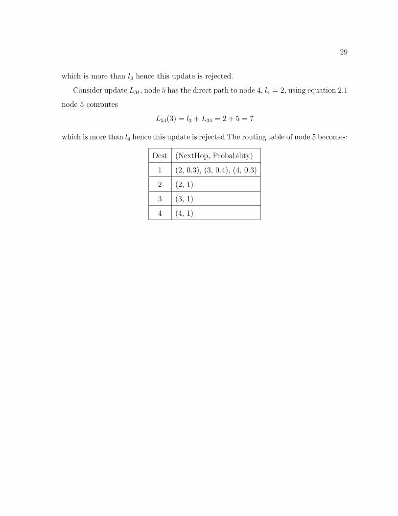
29
which is more than l3 hence this update is rejected.
Consider update L34, node 5 has the direct path to node 4, l4 = 2, using equation 2.1
node 5 computes
L54(3) = l3 + L34 = 2 + 5 = 7
which is more than l4 hence this update is rejected.The routing table of node 5 becomes:
Dest (NextHop, Probability)
1 (2, 0.3), (3, 0.4), (4, 0.3)
2 (2, 1)
3 (3, 1)
4 (4, 1)

Chapter 3
Simulation and Results
For the purpose of simulation, the routing algorithm was implemented in the Network
Simulator ns-2 [1, 11, 28]. Ns-2 is an open source network simulator which is written
in OTcl and C++. The parameters which were measured are Convergence Time,
Load on the Routers and Queue Size, all these parameters are described below. The
study comprised of the effect of the factors route computation delay, events occurring
in the network and frequency of updates on the above stated parameters. Extensive
simulations were performed to analyse the effects of these factors.
3.1 Implementation Details
The implementation of the algorithm on ns-2, comprises of three functional blocks.
• First block discovers a node’s neighbors by sending hello packets. Hello packets
were sent at at a fixed interval. Once a node receives a hello packet from its
neighbor it waits for a fixed amount of time called Holding Time, and if the
node does not gets another hello packet from that neighbor it declares it as
down.
• Second block sends updates to its neighbors. Updates are sent after fixed inter-
30
31
vals, with the exception when an event occurs then updates are sent immediately.
This helps the network to adapt quickly to changes in topology of the network.
• The third block computes the routing table based on the updates received.
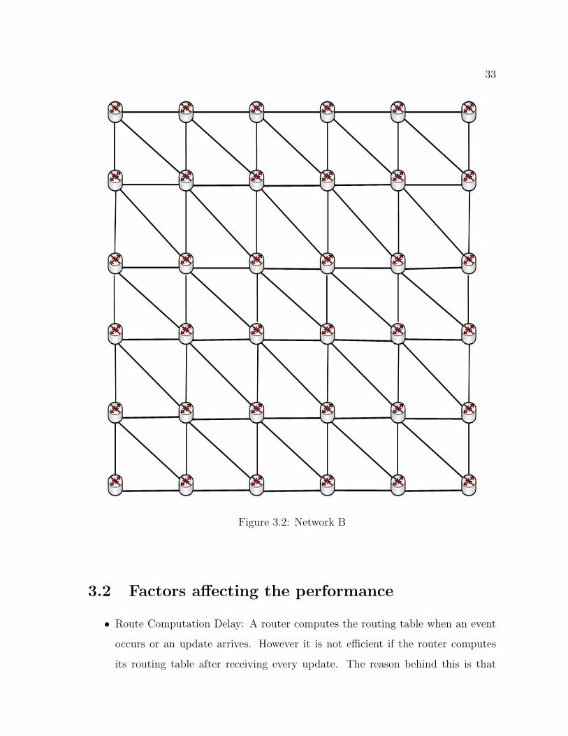
The simulations were performed on two different networks. They are shown in
figure 3.1 and figure 3.2. In all simulations the networks were given 10 seconds to attain
steady state, after the duration all the traffic was started and events were triggered.
The events are a link going up or down, or a change in cost of a link. All events were
triggered randomly.

32
Figure 3.1: Network A
33
Figure 3.2: Network B
3.2 Factors affecting the performance
• Route Computation Delay: A router computes the routing table when an event
occurs or an update arrives. However it is not efficient if the router computes
its routing table after receiving every update. The reason behind this is that
34
on occurrence of an event more than one updates are generated. Hence if on
receiving every update a router computes its routing table, then the load on the
router increases. To tackle this problem a Route Computation Delay is employed.
As the router receives an update it starts a timer and it computes its routing
tables when the time out happens. In this duration router will receive more
update packets and all will be used in computation of the routing table. A
low value of Route Computation Delay implies that all the updates may not be
incorporated and routing table will be computed many times, this increases the
load on the router. However a high value of this delay implies that the network
convergence time will increase which is undesirable.
• Events: Events as stated above are a link going up or down, or a change in cost.
Events were triggered at random instants. Events are used to analyze how the
algorithm works in a dynamically changing network like the internet.
• Frequency of Updates: Updates are sent to neighboring nodes to provide a con-
sistent view of the network’s topology. The routing algorithm running on each
node uses this topology to compute the routing table. It is desirable that updates
are sent frequently so as to incorporate the frequent changes occurring in the net-
work. However having a high frequency of updates or sending a high number of
updates per unit time increases the latency in the network because it increases
the number of queued packets queued on a router. Moreover a high frequency
of updates implies that the routing table will be calculated more frequently thus
increasing load on the routers.

35
3.3 Results
3.3.1 Convergence Time
For analysis convergence time [2] is defined as the time duration between occurrence
of an event and the time when each router in the network has updated its routing
table with the new information. A low convergence time is desired so that the network
can adapt to the changes in a network quickly. The goal of a routing algorithm is to
minimize the convergence time while keeping the load on the routers low.
Route computation delay is incorporated to involve several updates for computation
of routing table. Several simulations were carried out to calculate average Convergence
Time for the values of Route Computation Delay varying from 100 msec. to 2 sec. on
both Network A and Network B. Figure 3.3 shows the average convergence times vs
route computation delay for network A and figure 3.4 shows the same for network B.
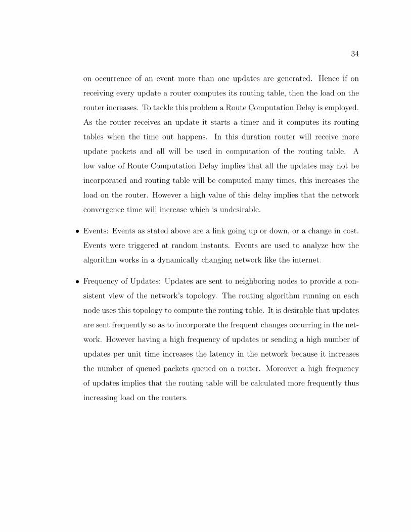
Simulations were carried out for various values of update frequencies. It can be ob-
served from the plots, for higher frequency of updates the algorithm converges quickly.

36
Figure 3.3: Convergence Time vs Route Computation Delay for Network A
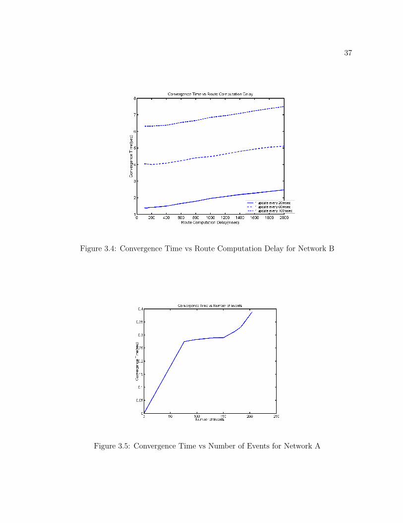
During the simulations events were randomly generated in time to observe the be-
havior of convergence time as the number of events vary. For this purpose links were
broken down and brought up again where the time instant when a link is broken down
and the duration for which the link remains down were kept random. Also cost of links
were changed randomly. Figure 3.5 and figure 3.6 show the variation of convergence
time as a function of number of events occurring in the network for network A and
network B respectively
37
Figure 3.4: Convergence Time vs Route Computation Delay for Network B
Figure 3.5: Convergence Time vs Number of Events for Network A

38
Figure 3.6: Convergence Time vs Number of Events for Network B
39
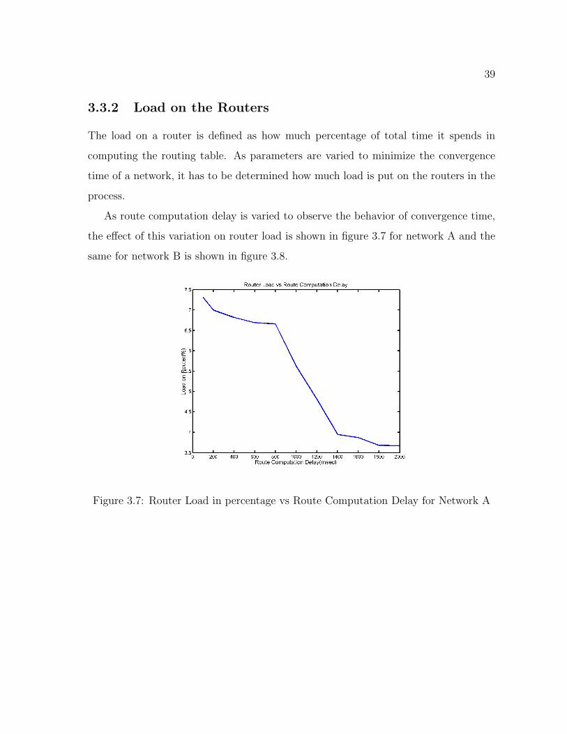
3.3.2 Load on the Routers
The load on a router is defined as how much percentage of total time it spends in
computing the routing table. As parameters are varied to minimize the convergence
time of a network, it has to be determined how much load is put on the routers in the
process.
As route computation delay is varied to observe the behavior of convergence time,
the effect of this variation on router load is shown in figure 3.7 for network A and the
same for network B is shown in figure 3.8.
Figure 3.7: Router Load in percentage vs Route Computation Delay for Network A

40
Figure 3.8: Router load in percentage vs Route Computation Delay for Network B
3.3.3 Size of the Queue
The size of the queue of any router is indicative of two things, how much load is on
the router and the congestion in the networks [10]. To minimize end to end latency
in a network the size of queue should be small. Queue size is mainly affected by the
frequency of updates. To observe this effect the queue size vs time of a router is plotted
for different values of update frequency. This is shown in figure 3.9.
The figure shows that for a high value of update frequency, less packets are queued
up. For lower values of update frequency update packets are queued up at the routers
hence the maximum size of the queue increases as update frequency is decreased.

41
Figure 3.9: Size of Queue on a router vs Time
Chapter 4
Conclusion
This thesis presented a probabilistic routing algorithm to overcome the problems faced
with selfish routing. For this purpose a new structure for the routing table and a
slightly different routing algorithm is proposed The algorithm deals with the problems
by providing multiple paths to a destination, where every path is assigned probability
according to the cost to the destination.
Performance of the algorithm was measured in terms of time taken to converge,
load on the routers and queue size. Convergence time is desired to be low for a
routing algorithm. Variation of convergence time was observed for different values
of route computation delay. It was observed that as route computation delay was
increased the algorithm took more time to converge. This is expected because the
less frequently routing table is computed the more time the network takes to adapt to
topology changes.
The performance of the algorithm was also studied in the event of changes occur-
ring. It was measured in terms of variation of convergence time with the number of
events. This helps in determining how the algorithm will perform when employed in
dynamically changing networks like the internet.
The load on the routers was also analysed in terms of variation of route computa-
tion delay. As the figures show load on the routers decreases with decrease in route
42
43
computation delay. This is because routers compute their routing tables less frequently.
Queue sizes were abalysed for various values of update frequencies. Queue size is
indicative of latency, because the number of packets queued at the router implies large
queuing delay.
4.1 Future Aspects
This algorithm does not supports hierarchical routing. For simulations to make the
algorithm scalable, entries in the routing table were removed if an update for that
destination does not arrive within a fixed interval.
This algorithm does not need a precise view of the network topology, hence it can
be applied to wireless networks as well. As of now no simulations have been carried
out to study the performance of the algorithm in wireless networks.

References
[1] Altman, E. and Jimenez, T. NS Simulator for Beginners.
[2] Altman, E. Boulogne, T. Azouzi, R.E. and Jimenez, T. A survey on networking
games. Telecommunication Systems. Nov 2000.
[3] Apostolopoulos, G. Guerin, R. Kamat, S.K. and Tripathi, S.K. Quality of Service
routing: A performance perspective. Proceedings of ACM SIGCOMM, pp. 1728,
September 1998.
[4] Bertsekas, D. and Gallager R. Data Networks. Prentice Hall of India, 1997.
[5] Cerf, V. and Kahn, R. A protocol for packet network intercommunication. IEEE
Transactions on Communications, 22(5), pp. 637648, May 1974.
[6] Chen, S. and Nahrsted, K. An overview of Quality of Service Routing for next
generation high-speed networks: problems and solutions . IEEE Networks, pp.
6479, November/December 1998.
[7] Cheng, C. A loop-free extended Bellman-Ford routing protocol without bouncing
effect . ACM Computer Communication Review, 19(4), pp. 224236, 1989.
[8] Cheng, C. Kumar, S.P.R. and Garcia-Luna-Aceves, J.J. A distributed algorithm
for finding K disjoint paths of minimum total length . Proceedings of the 28th An-
nual Allerton Conference on Communication, Control, and Computing, Urbana,
Illinois, Oct. 1990.
44

45
[9] Chinoy, B. Dynamics of Internet Routing Information . Proceedings of ACM SIG-
COMM, pp. 4552, September 1993.
[10] Cohen, J.E. and Jeffries, C. Congestion resulting from increased capacity in single-
server queuing networks. IEEE/ACM Transactions on Communications, 5(2), pp
305-310, 1997.
[11] Fall, K. and Varadhan, K. ns notes and documentation. The VINT Project 1998.
[12] Fuller, V. Li, T. Yu, J. and Varadhan, K. Classless interdomain routing (CIDR):
An address assignment and aggregation strategy. RFC 1519, September 1993.
[13] Gallager, R.G. A minimum delay routing algorithm using distributed computation.
IEEE Transactions on Communications pp 73-85, 1977.
[14] Garcia-Luna-Aceves J.J. A unified approach for loop-free routing using link states
or distance vectors. ACM Computer Communication Review, 19(4) pp. 212223,
1989.
[15] Mavronicholas, M. and Spirakis, P. The price of selfish routing. Proceedings of the
33rd Annual ACM symposium on the Theory of Computing, pp. 510-519, 2001.
[16] Nisan, N. Algorithms for selfish agents: Mechanism design for distributed compu-
tation. Proceedings of the 16th Annual Symposium on the Theoretical Aspects of
Computer Science, pp. 1-15, 1999.
[17] Orda, A. Rom, R. and Shimkin, N. Competitive routing in multiuser communica-
tion networks. IEEE/ACM Transactions on Networks, pp. 510-521 October 1993.
[18] Orda, A. and Libman, N. The designers’ perspective to atomic noncooperative
networks. IEEE/ACM Transactions on Networks, 7(6) pp. 875-884, 1999.
[19] Qiu, L. Yang, Y.R. Zhang, Y. and Shenker, S. On selfish Routing in internet like
environments. Proceedings of ACM SIGCOMM’03, Aug 2003.
46
[20] Roughgarden, T. Designing networks for selfish users is hard . Proceedings of the
42nd Annual Symposium on Foundations of Computer Science, pp. 472-481, 2001.
[21] Roughgarden, T. How unfair is optimal routing? . Proceedings of the 13nd Annual
Symposium on Discrete Algorithms, pp. 203-204, 2002.
[22] Roughgarden, T. The price of anarchy is independent of the network topology. .
Proceedings of the 34th Annual ACM Symposium on the Theory of Computing,
2002.
[23] Roughgarden, T. and Tardos, E. How bad is Selfish Routing? . Journal of ACM,
49(2), pp. 236-259, 2002.
[24] Shenker, S.J. Making greed work in networks: A game-theoretic analysis of switch
service disciplines . IEEE/ACM Transactions on Networking, 3(6), pp. 819831,
1995.
[25] Shenker, S.J. Clark, D. Estrin, D. and Herzog, S. Pricing in computer networks:
Reshaping the research agenda. . ACM Computer Communications Review, 26,
pp. 1943, April 1996.
[26] Tanenbaum, A.S. Computer Networks. Pearson Education, Asia-2003.
[27] Tistsiklis, J.N. and Bertsekas D. Distributed Asynchronous optimal routing in data
networks. IEEE Transactions on Automatic Control, April 1986.
[28] Network Simulator v2. http://www.isi.edu/nsnam/ns.