For peer review only
Detached Eddy Simulation on the Turbulent Flow in a Stirred
Tank
Journal: AIChE Journal
Manuscript ID: AIChE-11-13462.R1
Wiley - Manuscript type: Research Article
Date Submitted by the Author:
n/a
Complete List of Authors: Gimbun, Jolius; Universiti Malaysia Pahang, Faculty of Chemical & Natural Resources Engineering Rielly, Chris; Loughborough University, Department of Chemical Engineering Nagy, Zoltan; Loughborough University, Chemical Engineering Department Derksen, Jos; University of Alberta, Department of Chemical and Materials Engineering
Keywords: Computational fluid dynamics (CFD), Mixing
AIChE Journal
AIChE Journal
For peer review only
Detached Eddy Simulation on the Turbulent Flow in a Stirred Tank
J. Gimbun†a, b, C.D. Riellyb, Z.K. Nagyb, J.J. Derksenc
aFaculty of Chemical & Natural Resources Engineering, Universiti Malaysia Pahang, Lebuhraya Tun
Razak, 26300 Gambang, Pahang, Malaysia.
bDept. Chemical Engineering, Loughborough University, Leics, LE11 3TU, UK.
cDept. Chemical and Materials Engineering, University of Alberta, Edmonton, Alberta, Canada, T6G
2G6
Abstract
This paper presents a detached eddy simulation (DES), a large-eddy simulation
(LES), and a k-ε-based Reynolds averaged Navier-Stokes (RANS) calculation on
the single phase turbulent flow in a fully baffled stirred tank, agitated by a Rushton
turbine. The DES employed in this work is based on the Spalart-Allmaras
turbulence model solved on a grid containing about a million control volumes. The
standard k-ε and LES were considered in this study for comparison purposes.
Predictions of the impeller-angle-resolved and time-averaged turbulent flow have
been evaluated and compared with data from Laser Doppler Anemometry (LDA)
measurements. The effects of the turbulence model on the predictions of the mean
velocity components and the turbulent kinetic energy are most pronounced in the
(highly anisotropic) trailing vortex core region, with specifically DES performing
well. The LES – that was performed on the same grid as the DES – appears to lack
resolution in the boundary layers on the surface of the impeller. The findings
suggest that DES provides a more accurate prediction of the features of the
turbulent flows in a stirred tank compared to RANS-based models and at the same
time alleviates resolution requirements of LES close to walls.
Key words: DES, RANS, angle resolved, vortex core, power number, turbulent
kinetic energy
† Corresponding author
E-mail address: [email protected]
Page 1 of 55
AIChE Journal
AIChE Journal
123456789101112131415161718192021222324252627282930313233343536373839404142434445464748495051525354555657585960
For peer review only
1 Introduction
Stirred tanks are widely used in the chemical and biochemical process industries.
Mixing, fermentation, polymerisation, crystallisation and liquid-liquid extractions are
significant examples of industrial operations usually carried out in tanks agitated by
one or more impellers. The flow phenomena inside the tank are of great
importance in the design, scale-up and optimisation of tasks performed by stirred
tanks.
Although several advanced experimental methods such as Laser Doppler
Anemometry (LDA) and Particle Image Velocimetry (PIV) are capable of evaluating
the turbulent flow phenomena in stirred tanks, these methods have their specific
limitations. PIV and LDA techniques cannot be applied to opaque fluids, under
hazardous conditions, in non-transparent vessels or when the system is sensitive
to laser radiation. Computational Fluid Dynamics (CFD) presents an alternative
quantitative route of describing stirred tank flow, although modelling of dense
multiphase flows and fluids with complex rheology is still troublesome. In addition,
geometrical complexity and the in many cases turbulent nature of the flow make
that CFD results need to be critically assessed, e.g. by comparing them with
experimental data. Once sufficiently validated, CFD provides a powerful tool for
investigating flows and supporting process design at a lower expense than would
be required by a high-quality experimental facility.
Before dealing with multiphase flows, simulation of the single phase flow in stirred
tanks is necessary because the prediction of turbulent flows requires making
intricate modelling choices, specifically in complex domains with moving
boundaries such as the revolving impeller in a stirred tank. At the same time, good
prediction of turbulence quantities (turbulent kinetic energy, turbulent dissipation
rate) is important because they strongly influence small-scale processes (chemical
reactions, and disperse phase behaviour such as bubble coalescence and break-
up).
Modelling of turbulence in stirred tanks is challenging because the flow structures
are highly three-dimensional and cover a wide range of spatial and temporal
scales. The revolving impeller circulates the fluid through the tank and there are
three-dimensional vortices formed in the wakes behind the impeller blade1. Baffles
Page 2 of 55
AIChE Journal
AIChE Journal
123456789101112131415161718192021222324252627282930313233343536373839404142434445464748495051525354555657585960

For peer review only
at the tank wall prevent the liquid from performing a solid-body rotation, thus
enhancing the mixing, as well as generating strong axial and radial velocity
components.
Many researchers2-10 have studied Reynolds averaged Navier-Stokes (RANS)
based turbulence models (mainly k-ε models) applied to stirred tank flow. As a
general conclusion, these authors claim that CFD satisfactorily predicts mean flow
patterns as far as they are associated to axial and radial velocity components, but
either under- or over-predicts the flow in the circumferential direction and
turbulence quantities, such as the turbulent kinetic energy (k) and the turbulent
energy dissipation rate (ε). More elaborate RANS models such as the Reynolds
stress model (RSM) suffer from similar drawbacks3,7.
Predictions of tangential velocities have been a problem in simulations of stirred
tanks for some time. The tangential velocity fields averaged over all angular
impeller positions are usually fairly well represented by CFD. The issues are with
the impeller-angle resolved fields, and the associated vortex structures in the
wakes of impeller blades.
It is possible to fully resolve for the turbulent flow in a stirred tank by Direct
Numerical Simulation (DNS). Recently, DNS has been applied to predict the
turbulent flow in a stirred tank by Verzicco et al.11 and Sbrizzai et al.12. These
authors concluded that DNS predicts the turbulence related quantities such as
turbulent kinetic energy and turbulent energy dissipation rate much better than
RANS models. However, both works involved a low Reynolds number (Re = 1636;
a transitional flow) in an unbaffled tank, suggesting that DNS for a baffled stirred
tank at high Reynolds number is still far beyond the reach of current computer
resources.
The main limitation of RANS modelling of turbulently stirred tanks agitated by
Rushton turbines is the poor prediction of the turbulence related quantities such as
k and ε, and the impeller-angle resolved mean tangential velocity. It is well known
from the literature that large-eddy simulation (LES) is able to better predict the
time-averaged flow quantities, including those related to turbulence13-23. In a LES, a
low-pass filtered version of the Navier-Stokes equation is solved. The fluid motion
Page 3 of 55
AIChE Journal
AIChE Journal
123456789101112131415161718192021222324252627282930313233343536373839404142434445464748495051525354555657585960

For peer review only
at the sub-filter scales is taken care of by a model. It is a three-dimensional,
transient numerical simulation of turbulent flow, in which the large flow structures
are resolved explicitly and the effects of subgrid (or sub-filter) scales are modelled,
the rationale being that the latter are more universal and isotropic in nature. Large-
eddy simulations of stirred tank flow are computationally expensive. The
computational cost of an LES is largely dictated by spatial resolution requirements.
Away from walls, the spatial resolution needs to be such that the cut-off spatial
frequency of the low-pass filter falls within the inertial subrange of turbulence. In
addition, wall-boundary layers need to be sufficiently resolved. It is well understood
that the local Taylor-microscale is a good guide to prepare a grid for LES24.
Issues with LES related to boundary layers led to the idea of formulating a
turbulence model that is cheaper to run and better predicts turbulent flows, called
Detached Eddy Simulation (DES) or hybrid (RANS-LES) turbulence model. The
main idea of this approach is to perform LES away from walls where demands on
resolution are not that strong, and revert to RANS modelling where LES is not
affordable, i.e. in boundary layers. In strong turbulence, flow structures close to the
wall are very small25 and anisotropic. Thus an LES would need a very fine grid
within the boundary layer, which implies that the computational cost does not differ
appreciably from that of a DNS anymore26. On the other side, inadequate grid
resolution of boundary layers can severely degrade the quality of a large eddy
simulation. Therefore DES was proposed by Spalart et al.26 in an attempt to reduce
the computational cost as well as to provide a good prediction of turbulent flows,
containing boundary layers. A DES is an LES that transfers to a RANS-based
simulation in boundary layers, thus permitting a relatively coarse grid near walls. A
DES grid differs from a RANS grid and for that purpose Spalart27,28 has prepared a
detailed guide to mesh preparation.
To the authors' knowledge, DES has not yet been used for prediction of single-
phase, stirred tank flows in baffled vessels. The main objective of this work is to
assess the quality of DES predictions for stirred tank flow. For this, a detailed
comparison with experimental data in the vicinity of the impeller was performed
since in this region the flow is being generated, and here the effect of (in)adequate
wall-layer resolution would be most visible. Close to the impeller, boundary layers
detaching from impeller blades and associated vortex structures dominate the flow.
Page 4 of 55
AIChE Journal
AIChE Journal
123456789101112131415161718192021222324252627282930313233343536373839404142434445464748495051525354555657585960

For peer review only
Impeller-angle resolved data are necessary since their level of detail is required to
critically assess performance of DES. In addition to comparing the DES results with
experimental data, we also compare them with LES and k-ε results to judge the
performance of DES in relation to the latter two (more established and tested)
approaches.
Only a few modelling studies that assess the quality of impeller-angle-resolved
data with experiments are available in the literature. Li et al.9 have presented an
angle-resolved CFD and LDA comparison on turbulent flows produced by a retreat
curve impeller in a tank fitted with a single cylindrical baffle. These authors
employed a shear-stress-transport (SST) model in their work, which is a
combination of the k-ω model near the wall and the k-ε model away from the wall.
Tangential velocities and the turbulent kinetic energy were largely under-predicted
in their study. Yeoh et al.16 also have presented an angle-resolved comparison of
turbulent flows in a stirred tank. They employed a deforming mesh method with
LES and reported a good prediction of total kinetic energy. However, there was no
comparison made on the angle-resolved random kinetic energy. Hartmann et al.17
have presented an angle-resolved comparison of turbulent flows generated by a
Rushton turbine at a Reynolds number of 7300. The authors compared LES and
SST models in their work and concluded that LES predicts both angle-resolved and
time-averaged turbulent flow very well. The previous works of Yeoh et al.16 and
Hartmann et al.17 only presented a limited number of angle-resolved comparisons
of turbulent kinetic energy, i.e. for three different angles at a single radial position
only. Therefore, such a comparison may not sufficiently take into account the
details of the flow around the impeller blades, including trailing vortices.
An accurate prediction of both mean velocities and turbulent quantities in the
trailing vortex core is important, as this region plays an important role in the mixing
and phase dispersion. It is therefore interesting to investigate the capability of
various modelling approaches to predict the mean velocities and turbulence-related
quantities in the trailing vortex core.
Various aspects of stirred tanks modelling are discussed in this paper, including the
ability of turbulence models to predict the angle-averaged and angle-resolved
mean flows, turbulence characteristics, trailing vortices and the power number. The
Page 5 of 55
AIChE Journal
AIChE Journal
123456789101112131415161718192021222324252627282930313233343536373839404142434445464748495051525354555657585960
For peer review only
performance of the various models in predicting the turbulent flow in a single phase
stirred tank are identified, with specific attention for the potential of detached-eddy
simulations.
The organization of this paper is as follows: we start with introducing the flow
geometry, the computational grid, and then give a condensed description of the
three turbulence modelling approaches (viz. k-ε, LES, and DES) used in this study.
In the subsequent Results and Discussion section, first time-averaged velocity data
are discussed. Then we zoom in on the structure of the trailing vortex system
associated with the revolving impeller, and we compare the way this vortex system
is resolved by the various modelling strategies. The description of the vortex
system allows us to interpret the extensive set of impeller-angle-resolved velocity
profiles presented next. In the final section of the paper, we summarize and
reiterate the main conclusions.
2 Modelling approach
2.1 Tank geometry
The results presented in this work are related to a standard stirred tank
configuration, with the tank and impeller dimensions given by Derksen et al.29. The
system is a flat bottomed cylindrical tank, T = H = 0.288 m, with four equally
spaced baffles. A Rushton turbine with diameter, D = T/3, without a hub, was
positioned at a bottom clearance of C = T/3. The impeller blade and disk thickness
was t = 2 mm. The impeller was set to rotate with an angular velocity of N=3.14 rps
corresponding to a Reynolds number of 2
ReND
ν≡ = 29000 (with ν =1.0⋅10-6 m2/s
the kinematic viscosity of the working fluid which was water). In our coordinate
system, the level of z = 0 was set to correspond to the impeller disk plane.
2.2 Computational grid
GAMBIT 2.230 was employed to create an unstructured, non-uniform multi-block
grid with the impeller (rotating) and static zones being separated by an interface to
enable the use of the Multiple Reference Frame (MRF) or Sliding Grid (SG)
techniques. The computational grid for the RANS modelling was defined by
Page 6 of 55
AIChE Journal
AIChE Journal
123456789101112131415161718192021222324252627282930313233343536373839404142434445464748495051525354555657585960

For peer review only
516000 (516k) of structured, non-uniformly distributed hexahedral cells
representing (with view to symmetry) only a half-tank domain. A local grid
refinement containing 212k cells was applied in the rotating zones to better resolve
this highly turbulent region.
The grid for a DES cannot make use of the half-tank and periodic boundary
conditions, because here the simulation is fully unsteady and not symmetric. Thus
the existing grid was extended to a full tank grid for the DES. As a result the
extended grid of the whole tank domain contained about a million control volumes
(1010k). The DES grid was prepared according to Spalart27,28 with vyuy T≡+
ranged from 1 to 33 around the walls defining the impeller. The Tu , y and v are
the friction velocity, distance from the nearest wall and the kinematic viscosity,
respectively. A grid adaptation is applied around the impeller at 0 < 2r/D < 1.7 to
control the mesh size in this highly turbulent region at max(∆x, ∆y, ∆z) < 0.7 mm
(=7.3 x 10⁻³D).
The grid cell size in the impeller region in the current work is smaller than 0.015D
which is finer than the locally refined grid (0.023D) used by Revstedt et al.13, who
reported a good prediction of turbulence flow using LES. In addition, the Taylor-
microscale is well resolved in the impeller discharged region where 80% of the
turbulent kinetics energy dissipates14. However, the grid close to impeller wall are
not resolved since the main focus of this work is to evaluate the strength of DES for
predicting turbulence flow using coarser grid than that for LES. According to
Derksen et al.29 a proper grid for stirred tanks modelling should be able to resolve
the trailing vortex behind the impeller blade. They recommended using at least 8
nodes along the impeller height (corresponding to 0.025D) to resolve the trailing
vortex for RANS modelling. The trailing vortex is an important flow feature in stirred
tanks which significantly affects prediction of the turbulence and mean flow. In this
work, 12 nodes along the impeller blade height were assigned for the RANS
modelling and 23 nodes were used for the LES and DES modelling. The grid
prepared in this work is capable of resolving accurately the radial and axial trailing
vortex, as shown in section 3.2, thus further confirming its suitability.
Page 7 of 55
AIChE Journal
AIChE Journal
123456789101112131415161718192021222324252627282930313233343536373839404142434445464748495051525354555657585960

For peer review only
2.3 Turbulence modelling and discretisation
The selection of a turbulence model for stirred tank simulation is very important,
especially when dealing with baffled tanks at high Reynolds numbers (strong
turbulence). LES is of course an excellent model, but it is still computationally
expensive to run on a personal computer, for instance, Delafosse et al.22 needs 80
days to run LES on a AMD Opteron workstation. Whereas, comparatively new
turbulence models such as DES need to be validated before they can be applied
routinely to stirred tank modelling. Therefore the predictive capabilities the most
commonly used RANS model i.e. the standard k-ε as well as DES and LES, on
turbulent flows in a single-phase stirred tank have been extensively compared in
this study. These models are described in more detail below.
The standard k-ε model is based on transport equations for the turbulent kinetic
energy and its dissipation rate. Transport equations for k and ε for all k-ε variant
models can be generalised as follow:
( ) ( ){ {
ndestructioproduction
diffusionconvectionderivativetime
ρερσµ
µρρ
−+
∂∂
+
∂∂
=∂∂
+∂
∂k
ik
t
i
i
i
Px
k
xku
xt
k
444 3444 2143421321
(1)
and
( ) ( ){
termsource
diffusionconvectionderivativetime
εε
εσµ
µερρε
Sxx
uxt i
t
i
i
i
+
∂∂
+
∂∂
=∂∂
+∂
∂
444 3444 2143421321
(2)
The turbulent (eddy) viscosity, tµ , is obtained from:
ερµ µ
2k
Ct = (3)
The relation for the production term, Pk, for the k-ε model is given as:
i
j
j
i
i
j
tkx
u
x
u
x
uP
∂
∂
∂∂
+∂
∂= µ (4)
For the standard k-ε model the source term, Sε, is given by:
−=
kCP
kCS k
2
21
εερ εεε (5)
The model constants are31: 44.11 =εC 92.12 =εC 09.0=µC 1=kσ 3.1=εσ derived
from correlations of experimental data.
Page 8 of 55
AIChE Journal
AIChE Journal
123456789101112131415161718192021222324252627282930313233343536373839404142434445464748495051525354555657585960

For peer review only
In LES it is assumed that the large eddies of the flow are dependent on the flow
geometry and boundary conditions, while the smaller eddies are self-similar and
have a universal character. Thus, in LES the large unsteady vortices are solved
directly by the filtered Navier-Stokes equations, while the effect of the smaller
universal scales (sub-grid scales) are modelled using a sub-grid scale (SGS)
model. The filtered Navier-Stokes equation is given by:
( )ij
SGS
ij
j
i
ji
j
i
x
p
xx
uuu
xt
u
∂∂
−∂
∂−
∂
∂=
∂∂
+∂
∂ τ2
2
Re
1 (6)
where SGS
ijτ is the subgrid-scale (SGS) stress modelled by:
ij
SGS
tij
SGS
kk
SGS
ij Sµδττ 23
1−=− (7)
The SGS
tµ is the SGS turbulent viscosity, and ijS , is rate-of-strain tensor for the
resolved velocity field defined as:
∂
∂+
∂∂
=i
j
j
iij
x
u
x
uS
2
1 (8)
The overbars in eq.(6) to eq.(9) denote resolved scale quantities rather than time-
averages. The most commonly used SGS model is the Smagorinsky32 model,
which has been further developed by Lilly33. It compensates for the unresolved
turbulent scales through the addition of an isotropic turbulent viscosity into the
governing equations. In the Smagorinsky-Lilly model the turbulent viscosity is
modelled by:
SLs
SGS
t
2ρµ = (9)
where Ls is the mixing length for sub-grid scales and ijijSSS 2= . Ls can be
calculated from:
( )31,min VCdL ss κ= (10)
where κ = 0.42, d is the distance to the nearest wall, Cs is the Smagorinsky
constant, and V is the volume of the computational cell. The Smagorinsky constant
was set to 0.1 which is a commonly applied value for shear-driven turbulence. The
Smagorinsky constant was set at 0.2 in the newer version of Fluent Ansys R13,
which could have been motivated by findings by Delafosse et al.22 who shows a
better prediction of turbulent dissipation rate from LES can be obtained by
adjusting the constant Cs in the Smagorinsky model from 0.1 to 0.2. A LES was
Page 9 of 55
AIChE Journal
AIChE Journal
123456789101112131415161718192021222324252627282930313233343536373839404142434445464748495051525354555657585960

For peer review only
performed in this work to evaluate the effect of unresolved eddies near the impeller
wall on the turbulence and mean velocities predictions. It has to be noted that the
y+ around the impeller wall in this work ranged from 5 to 40 which is not well-
resolved for LES. To the best of our knowledge, the effect of the unresolved eddies
near the impeller wall on the LES prediction has not been evaluated
comprehensively for a stirred tank flow, especially not in terms of angle-resolved
flow quantities.
DES as mentioned earlier belongs to a class of a hybrid turbulence models which
blend LES in flow regions away from boundary layers with RANS near the wall.
This approach was introduced by Spalart et al.26 in an effort to reduce the overall
computational effort of LES modelling by allowing a coarser grid within the
boundary layers. The DES employed in this work is based on the Spalart-Allmaras
(SA) model34.
The SA one-equation model solves a single partial differential equation (eq. 11) for
a variable v~ which is called the modified turbulent viscosity. The variable v~ is
related to the eddy viscosity by eq. 12 with additional viscous damping function fv1
to ensure the eddy viscosity is predicted well in both the log layer and the viscous-
affected region. The model includes a destruction term that reduces the turbulent
viscosity in the log layer and laminar sub-layer. The transport equation for v~ in
DES is:
( ) ( ) v
j
b
jjv
vi
i
Yx
vC
x
vv
xGuv
xv
t−
∂∂
+
∂∂
+∂∂
+=∂∂
+∂∂
2
2~
~~)~(
1~~ ρρµσ
ρρ (11)
The turbulent viscosity is determined via:
v
v
Cffv
v
vvt
~,,~
3
1
3
3
11 ≡+
== χχ
χρµ (12)
where v = µ/ρ is the molecular kinematic viscosity. The production term, Gv, is
modelled as:
1
222211
1,~~
,~~
v
vvbvf
ffdk
vSSvSCG
χχ
ρ+
−=+≡= (13)
S is a scalar measure of the deformation rate tensor which is based on the vorticity
magnitude in the SA model. The destruction term is modelled as:
Page 10 of 55
AIChE Journal
AIChE Journal
123456789101112131415161718192021222324252627282930313233343536373839404142434445464748495051525354555657585960

For peer review only
( )22
6
2
61
6
3
6
6
3
2
1 ~
~,,
1,
~
dkS
vrrrCrg
Cg
Cgf
d
vfCY w
w
wwwwv ≡−+=
++
=
= ρ (14)
The closure coefficients for SA model34 are 1355.01 =bC , 622.02 =bC , 3
2~ =vσ ,
1.71 =vC , ( )
v
bbw
C
k
CC
~
2
2
11
1
σ+
+= , 3.02 =wC , 0.23 =wC , 4187.0=k .
In the SA model the destruction term (eq. 14) is proportional to ( )2/~ dv . When this
term is balanced with the production term, the eddy viscosity becomes proportional
to 2~dS . The Smagorinsky LES model varies its sub-grid-scale (SGS) turbulent
viscosity with the local strain rate, and the grid spacing is described by 2~∆SvSGS α
in eq.(9), where ∆ = max(∆x, ∆y, ∆z). If d is replaced with ∆ in the wall destruction
term, the SA model will act like a LES model. To exhibit both RANS and LES
behaviour, d in the SA model is replaced by:
( )∆= desCdd ,min~
(15)
where Cdes is a constant with a value of 0.65. Then the distance to the closest wall d
in the SA model is replaced with the new length scale d~
to obtain the DES. The
purpose of using this new length is that in boundary layers where ∆ by far exceeds
d, the standard SA model applies since dd =~
. Away from walls where ∆= desCd~
,
the model turns into a simple one equation SGS model, close to Smagorinsky’s in
the sense that both make the mixing length proportional to ∆. The Smagorinsky
model is the standard eddy viscosity model for LES. On the other hand, this
approach retains the full sensitivity of RANS model predictions in the boundary
layer. This model has not yet been applied to predict stirred tank flows. Applying
DES and assessing its performance in relation to experimental data and other
turbulence modelling approaches is the main objective of the current study.
2.4 Modelling strategy
A multiple reference frame (MRF) model36 was applied to represent the impeller
rotation for all the RANS simulations, with a second-order discretisation scheme
and standard wall functions. The bounded central differencing (BCD) scheme was
applied for spatial discretisation of the momentum equations for the DES
modelling, and time-advancement was achieved by a second-order accurate
Page 11 of 55
AIChE Journal
AIChE Journal
123456789101112131415161718192021222324252627282930313233343536373839404142434445464748495051525354555657585960

For peer review only
implicit scheme. The central differencing scheme is an ideal choice for LES due to
its lower numerical diffusion. However, it often leads to unphysical oscillations in
the solution field35. The BCD scheme was introduced to reduce these unphysical
oscillations. BCD blends the pure central differencing scheme with first- and
second-order upwind schemes. The first-order scheme is applied only when the
convection boundedness criterion is violated35.
The transient impeller motion for the DES study was modelled using the sliding
mesh scheme. PRESTO37 was applied for pressure-velocity coupling for all cases,
as it is optimised for swirling and rotating flow35. The DES modelling was initialised
using the data from a k-ε simulation. A text user interface command was used to
generate the instantaneous velocity field out of the steady-state RANS results. This
command must be executed before DES is enabled to create a more realistic initial
field for the DES run. This step is necessary to reduce the time needed for the DES
simulation to reach a statistically steady-state. Apart from the DES modelling, a
LES study was also carried out for comparison. The LES and DES were solved
using the same grid because the main aim of this work was to carry out the
simulation using a fairly coarse grid (y+ ~ 20), where the DES should be working
well. The LES was initialised using the final data from the DES simulation.
The time step and the number of iterations are crucial in both DES and LES
modelling because they involve a transient solution. The time step must be small
enough to capture all flow features induced by the motion of the impeller blades.
Selection of the time step would not be clear without a review of some recent LES
studies on stirred tanks. The time steps for LES simulations taken from the
literature were normalised with the impeller speed (∆tN) to make the value
dimensionless. Revstedt et al.13 employed a ∆tN of 0.0027, Alcamo et al.23 used a
∆tN of 0.0083 and Yeoh et al.16 employed a ∆tN of 0.0046. FLUENT35 recommends
that in one time step the sliding interface should move by no more than one grid
spacing in order to get a stable solution. In this study a ∆tN of 0.00278 was
employed throughout the final simulation corresponding to 1˚ impeller movement
for the LES and DES simulation. The grid size at the sliding interface was set at
0.002 m and the circumference of the interface was 0.69 m. Thus one grid cell
movement per time step would require a ∆tN of 0.00289 which is larger than the
Page 12 of 55
AIChE Journal
AIChE Journal
123456789101112131415161718192021222324252627282930313233343536373839404142434445464748495051525354555657585960

For peer review only
one employed in this work. About 7 s of actual time was simulated corresponding
to about 22 impeller revolutions. Prior to that, about 145 impeller revolutions had
been simulated using a ∆tN of 0.00833 corresponding to 3˚ of impeller movement.
The instantaneous velocity and torque acting on the impeller surface were
monitored throughout the simulation, and the data presented in this work were
taken after the statistical convergence has been achieved. About 10 s of actual
time has been simulated for a time step corresponding to 1˚ impeller movement for
the LES modelling starting from the final DES flow field. The three instantaneous
velocity components were recorded at every time step at various monitoring points
(analogous to LDA measurements) and data extraction on a plane (analogous to
3D PIV as all the three dimensional velocity component can be obtained). Post-
processing of the DES and LES data were performed using a Visual Basic code
embedded in MS Excel.
3 Results and discussions
The CFD simulations of a Rushton turbine described in this paper were compared
with the experimental LDA results reported by Derksen et al.29. The three
component LDA data used for these validation purposes were angle-resolved
mean and fluctuating velocities taken at 3˚ intervals of blade rotation, starting from
1˚ behind the blade (see Derksen et al.29 for details). All data of the mean velocity,
k and ε were made dimensionless by dividing them by tipV , 2
tipV or N3D
2,
respectively. The LDA data were processed as time-averaged, angle-resolved
mean and turbulence quantities.
A grid analysis was not performed in this paper but the prepared grid was assumed
to be fine enough to yield a grid independent solution. According to Derksen and
Van den Akker14, about 80% of the turbulence generated by a rotating impeller is
dissipated within the impeller swept volume and the impeller discharge region.
Derksen et al.29 also stated that the trailing vortex behind the impeller blade must
be well resolved in order to obtain a reasonable prediction of the turbulence and
mean velocities. They suggested at least 8 nodes should be placed along the
impeller blade height to resolve the trailing vortex, and the grid employed in this
work was prepared sufficiently fine with 12 nodes for the RANS simulation and 23
nodes for the DES and LES simulation (see earlier discussions in section 2.2). A
Page 13 of 55
AIChE Journal
AIChE Journal
123456789101112131415161718192021222324252627282930313233343536373839404142434445464748495051525354555657585960

For peer review only
grid analysis performed in our previous work38 based on the grid refinement around
the impeller and its discharge region also confirmed the suitability of the prepared
grid to produce a grid independent solution.
CFD results for the time-averaged and impeller-angle-resolved single phase
turbulent flow are discussed extensively in this section. All results presented are
taken from a well converged simulation, where the normalized residuals have fallen
below 1 x 10⁻³ for all RANS model simulations. RANS was chosen in this work
instead of URANS because there is a limited difference from the result obtained
using either URANS or RANS16,17. Moreover, URANS requires longer iteration
because they require a solution from unsteady sliding mesh. Of course there is no
such convergence criterion for the transient simulations using DES and LES.
However a sufficient number of iterations per time step (up to 35 iterations per time
step) have been applied to make sure the residuals fell below 1 x 10⁻³ at each time
step. The results for the DES and LES presented here were averaged over the 4
final impeller revolutions after the statistical convergence on the instantaneous
velocity was achieved. Four impeller revolutions are sufficient for post-processing if
the flows are already in pseudo-steady condition (e.g. 2.5 revolutions used by
Alcamo et al.23).
Angle-resolved result near the impeller tip and in the impeller out stream (from 2r/D
= 1.1 to 1.52) for mean velocities and turbulent kinetic energy are compared with
the angle-resolved LDA experiments. A broad range of angle-resolved
comparisons are necessary to capture the effect of the trailing vortex core on the
prediction of mean and turbulent flow quantities. With a view to extending our work
to multiphase systems, the accuracy of such CFD prediction in multi-phase flows
might be critically dependent on proper simulation of the trailing vortex core. A
detailed comparison between the CFD predictions and the published
measurements, very close to the impeller tip is presented in this section. The
effects of the vortex core on the prediction of mean and turbulent flows are
accounted by comparing the angle-resolved data and the CFD predictions at
different radial positions. Besides the mean and turbulent flow, the axial and radial
position of the vortex core were also deduced from the CFD results and compared
with Derksen et al.’s29 data.
Page 14 of 55
AIChE Journal
AIChE Journal
123456789101112131415161718192021222324252627282930313233343536373839404142434445464748495051525354555657585960

For peer review only
3.1 Time-averaged predictions
Generally, predictions of the LES, DES and k-ε models employed in this study for
the time-averaged velocity components (axial, radial and tangential) were in good
agreement with Derksen et al.’s29 LDA measurements with error approximately
10% as shown in Fig. 1. This shows that it is generally easy to predict the mean
flow in a stirred tank. Although some discrepancies of the CFD predictions were
observed for the impeller-angle-resolved comparisons (as will be discussed bein
section 3.3), they apparently where averaged out in the time-averaged results: The
CFD predictions are generally good for all angles except for some positions around
the trailing vortex core and these discrepancies appear to be marginal when
averaged over all azimuthal positions.
The velocity fluctuations in a stirred tank may be categorised as periodic (related to
the blade passage) and random (turbulence). As a result, the kinetic energy
associated to the fluctuations can be divided in a coherent (kcoh) and random (kran)
part. The total kinetic energy (ktot) in the velocity fluctuations is therefore:
( )22
2
1iirancohtot uukkk −=+= (16)
where iu is the instantaneous velocity in direction i and iu is the time-averaged
velocity. The averages are over all velocity samples irrespective of the angular
position of the impeller and the summation convention is applied over the repeated
suffix i. The random part of the kinetic energy can be determined if angle-resolved
data are available:
−=
22
2
1
θθ iiran uuk (17)
with θ
denotes the average value at impeller angular position θ. The overbar in
equation (17) denotes averaging over all angular positions (equivalent to time-
averaging).
Predictions of the angle-averaged rank by the k-ε model are about 20% lower than
Derksen et al.’s data which is consistent to many other previous works7,16,17,22. This
is worthwhile highlighting since to the best of our knowledge the k-ε model
generally underpredicts rank by more than 30%. An exception is due to Nere et
al.39, who empirically adjusted the values of the standard constants in the k-ε model
Page 15 of 55
AIChE Journal
AIChE Journal
123456789101112131415161718192021222324252627282930313233343536373839404142434445464748495051525354555657585960

For peer review only
in their study. We do not consider this good practice, since these constants have
already been tuned using experimental data and should be retained. The relatively
good predictions of rank by the RANS model in this study are believed to be
attributable to the application of a very fine grid around the impeller.
No comparisons can be made for the ktot prediction by the RANS model, because
the impeller is actually ‘frozen’ at a single position in the MRF model. The DES
yielded the best prediction of the ktot (see Fig. 2) and rank (see Fig. 3) with error of
less than 5% although prediction by LES away from the impeller (2r/D = 1.52) were
as good as those obtained from DES. The LES predictions were not very good
close to the blade tip (2r/D = 1.1) with error up to 20%. This could be due to under-
resolved eddies near the impeller wall. The grid was prepared for DES (y+ ~ 20)
and (as mentioned earlier) the LES modelling was carried out to compare DES and
LES and assess if and to what extend DES improves predictions by better
representing boundary layers. At positions closer to the impeller (2r/D = 1.1) the
DES is capable of producing the double peak in ktot often observed experimentally
whilst the LES fails to show this (although the LES predictions of ktot are still close
to the experimental measurements). Similar trends were also observed for the rank
predictions where the LES fails to predict correctly the rank at 2r/D = 1.1. The ktot is
predicted reasonably well by the LES because the ktot is calculated mainly from
periodic velocity fluctuation due to the impeller passage, whilst rank depends only
on the velocity fluctuations due to the turbulent flow, which explains the poor
prediction at 2r/D = 1.1. The result for rank demonstrates that the grid prepared in
this work is not optimal for LES, but it is good for DES. The DES does not need to
resolve the small eddies in the boundary layer, since the DES turns into a RANS
model in this region and hence works well even for a coarser grid. There are some
other studies on LES prediction of turbulent flow in stirred tanks using a relatively
coarse grid (e.g. Yeoh et al.16) and they report a good prediction of the turbulent
kinetic energy. However, they only presented the ktot which includes the periodic
turbulent fluctuation due to the blade passage and they have not presented any
comparison for the rank prediction alone. Such an LES study with a coarser grid
Page 16 of 55
AIChE Journal
AIChE Journal
123456789101112131415161718192021222324252627282930313233343536373839404142434445464748495051525354555657585960

For peer review only
may not resolve the flow near the boundary layer well enough and it may not be
able to resolve the rank around the impeller discharge.
Modelling of gas-liquid stirred tank is among the potential application of this study,
which require good predictions of turbulence flow, since they affect prediction of
the local bubble size. Correct prediction of the local bubble size is important as
they affect directly the hydrodynamics of gas-liquid stirred tank. In this particular
application, it is acceptable to have up to 20% error on the turbulence flow
prediction since the breakage and coalescence kernel used by the population
balance model will not amplify them further. For instance, the commonly used
breakage and coalescence kernel for bubble i.e. Luo40, Luo and Svendsen41 and
Prince and Blanch42 has the kinetics of breakage and coalescence depend on εa,
where |a| is small (0.25 or 0.33). So a 20% error in ε gives rise to less than 5%
error in the kinetic rate. In this work prediction on the mean and turbulence flow is
hardly more than 10% for the DES and therefore, should be acceptable. Moreover,
most of the breakage occurs in regions around the impeller, where the turbulence
flow is well predicted.
3.2 Identification of the vortex core
The vortex core is an important flow feature which needs to be well represented as
it potentially has a great influence on the overall turbulent flow in a stirred tank and
(in multiphase applications) the dispersed phase (bubbles, drops, particles) mixing.
For instance, the trailing vortices play a crucial role in determining the gas
accumulation behind the impeller43, meanwhile Derksen et al.29 find that it is
impossible to predict accurately the turbulent flow in stirred tanks without resolving
accurately the trailing vortices. In turn this affects the pumping and power
dissipation capacity of the impeller and thus significantly affects the performance of
a gas-liquid stirred reactor. Furthermore, the trailing vortices were associated with
high levels of turbulent activity and high velocity gradients and thus play an
important role in the mixing capability of a stirred tank44.
CFD predictions of the radial position of the trailing vortex core have been
published by many researchers14,23,45. However, most of the previous studies only
consider a single vortex core position (either the upper or lower); the exception is
by Derksen and van den Akker14 who considered both cores. In addition, there has
Page 17 of 55
AIChE Journal
AIChE Journal
123456789101112131415161718192021222324252627282930313233343536373839404142434445464748495051525354555657585960

For peer review only
been no extensive CFD comparison made on the axial position of the vortex core
with experimental measurements.
A detailed experimental study of the vortex core has been reported previously by
Escudie et al.46 based on the axial and radial positions of the vortex core deduced
using three different methods. The first method was called a “null velocity method”:
the vortex core was obtained simply by connecting the points at which the axial
velocity was equal to zero, as proposed by Yianneskis et al.1. The second method
was called the “vorticity method” in which the vortex core position was obtained by
connecting the points of maximum vorticity magnitude. The third method, namely
2λ , was proposed by Jeong and Hussain47 and was based on the presence of a
minimum local pressure in a plane perpendicular to the vortex axis. Escudie et al.46
found that all three methods gave almost identical curves for the vortex radial
position, however, the null velocity method gave a slightly different result compared
to both vorticity and 2λ method for the axial position. The vortex core in this work
was determined by using the vorticity method, as it is relatively simple to perform
and shows similar results as the 2λ method.
Data on several planes behind the impeller were exported to independent post-
processing software, SURFER 8, to avoid parallax error from visual assessments
of the maximum vorticity position. The vorticity surface plots on a series of r-z
planes at different blade angles were obtained using SURFER 8 and the positions
of the vortex core were determined using the build-in digitiser. Post-processing of
the DES data was not as straightforward as for the RANS models, as the
instantaneous vorticity magnitudes in the respective r-z planes (at blade angles 3˚
to 50˚) have to be averaged first before further analysis can be done. A total of 540
instantaneous surface data sets at each blade angle were averaged using Visual
Basic code embedded in MS Excel.
Fig. 4 shows a comparison of the radial positions of the predicted and the
experimental lower and upper vortex cores. The k-ε model provide reasonably
good agreement (approx. 7% error) with the results from Derksen et al.29 for the
upper vortex core, but are not as good for the lower vortex core when compared to
measurement by Yianneskis et al.1 with deviation more than 15%. Comparisons
are also made with experimental data from other authors i.e. Escudie et al.46,
Page 18 of 55
AIChE Journal
AIChE Journal
123456789101112131415161718192021222324252627282930313233343536373839404142434445464748495051525354555657585960

For peer review only
Yianneskis et al.1, Lee and Yianneskis44 and Stoots and Calabrese48. Escudie et
al.46, Yianneskis et al.1 and Lee and Yianneskis44 worked on a geometrically similar
vessel (D = C = T/3) to the one evaluated in this paper but with slightly different
tank diameters: T = 0.45 m for Escudie et al.46, T = 0.294 m for Yianneskis et al.1
and T = 0.1 m for Lee and Yianneskis44. According to Lee and Yianneskis44, tanks
with geometrically similar dimensions may be able to produce a reasonably similar
trailing vortex core, concluding from their results from tanks with diameter of T =
0.1 m and T = 0.294 m. Meanwhile, Stoots and Calabrese’s48 work was based on a
tank with diameter T = 0.45 m and C = T/2. The CFD predictions in this work were
only compared to those obtained using stirred tank with impeller to tank diameter
ratio of D = T/3 to eliminate an incorrect comparison as the vortex core may also
be affected by the D/T ratio. Data from these various authors did show some
differences, but they are in close agreement to those from Derksen et al.29. The
DES model gives a good prediction of both the lower and upper vortex core (less
than 5% error); slightly better than the k-ε model. It is known that the trailing
vortices are amongst the most anisotropic region in a stirred tank, thus demanding
the use of a more elaborate turbulence model such as DES or LES. Predictions of
LES for the radial position of upper and lower trailing vortices are also in good
agreement (approx. 5% error) with experimental data. However, the maximum
errors for the LES predictions are slightly bigger than those of DES as they are
affected by unresolved eddies close to impeller wall.
There are several viewpoints related to the axial position of the vortex core. For
example, Yianneskis1 claimed that the upper vortex core moves at a constant axial
position from the top of the impeller at 2z/W = 1, whilst Derksen et al.29 claimed that
the lower vortex core moves at a constant axial position of 2z/W = -0.52. Escudie et
al.46 found that both the lower and upper vortex core move axially upwards with the
lower vortex crossing the impeller centreline (2z/W = 0) and moving towards 2z/W =
0.3; the upper vortex appeared not to move further than 2z/W = 1. Stoots and
Calabrese48 have studied the axial position of the lower vortex core and they claim
that the core was at 2z/W = -0.6 close to the impeller blade, while at larger blade
angles, the core moves towards 2z/W ~ -1. Stoots and Calabrese48 findings suggest
the impeller placement play a big role on the axial position of the lower vortex core
as it was found to move downward instead of moving forward when the impeller
Page 19 of 55
AIChE Journal
AIChE Journal
123456789101112131415161718192021222324252627282930313233343536373839404142434445464748495051525354555657585960

For peer review only
positioned at T/2 instead of T/3. It is therefore interesting to investigate the
capabilities of CFD to predict the axial position of the vortex core in stirred tanks,
while bearing in mind the variability of the experimental findings.
Fig. 5 shows the predicted axial positions of the vortex core behind the Rushton
disk turbine blades. The DES model are in good agreement (less than 10% error)
with Escudie et al.’s46 experiments that involved a similar geometry as the present
one (impeller bottom clearance and impeller size is T/3). The upward movement of
both trailing vortex pairs is successfully predicted by the DES model. The upward
vortex movement is as expected, since it is well known that the discharge flow of
the Rushton turbine placed at T/3 bottom clearance is inclined slightly upward. It
was also noted that the upward movement of the lower vortex core was greater
than the upper vortex core. The k-ε model is less successful in predicting the axial
position of the vortex core correctly with error up to 30%. Prediction from LES is
reasonable for the lower vortex core (approx. 15% error) but is generally poor for
the upper vortex core (approx. 30% error). As mentioned earlier this is attributed by
unresolved eddies close to impeller wall. The poor predictions of trailing vortex core
by LES also explains why LES fails to predict the double peak turbulent kinetics
energy close to impeller in Fig. 2.
3.3 Prediction of the impeller-angle-resolved flow
Prior to discussion of the angle-resolved comparisons (in Figs. 6 to 9), it is
important to relate to the position of the trailing vortices behind the impeller. For
reference, two radial positions of 2r/D = 1.3 and 1.52 are shown. At an angle of
around 30˚ to 50˚ vortex cores are near 2r/D = 1.3 and by around 60˚ they have
reached 2r/D = 1.52. Predictions of the turbulent kinetics energy especially by the
k-ε models are highly affected by the cores of the trailing vortices.
Generally, the angle-resolved tangential velocities appear to be either under- or
over-predicted in the trailing vortex core using the RANS models but the agreement
is fairly good. The deviations might be attributed to the strongly anisotropic flow
within the trailing vortices, thus demanding the application of a more elaborate
turbulence model like DES, or LES. The DES model has great potential to predict
accurately the tangential velocity just before the vortex core, as shown in Figs. 6A
(at 19˚) and 6B (at 40˚ and 49˚). This is due to the fact that the large eddies are
Page 20 of 55
AIChE Journal
AIChE Journal
123456789101112131415161718192021222324252627282930313233343536373839404142434445464748495051525354555657585960

For peer review only
resolve directly by DES away from boundary layer. Predictions of the k-ε model for
the angle-resolved tangential velocity are also in reasonable agreement to Derksen
et al.’s29 measurements with approximately 10% deviation. The Vθ are predicted
well within the centre region of the vortex core when the DES and k-ε models are
employed but predictions by LES is not very good. Finding from this work suggest
that k-ε model performed better than unresolved LES.
Predictions of angle-resolved radial velocity are also affected by the vortex core in
a fashion similar to the angle-resolved tangential velocity as shown in Figs. 7A and
7B. Of the turbulence models tested, DES was found to have the upper hand in
predicting the angle-resolved radial velocity with error consistently around 10%.
However, predictions of the k-ε were also in close agreement (approx. 10% error)
with the experimental data. Predictions by LES is not outstanding with deviation up
to 50%, especially within the vortex core close to the impeller tip as shown in Fig.
7A (at 31˚ and 40˚).
Figs. 8A and 8B show the prediction of angle-resolved axial velocities. Predictions
of k-ε model is in reasonably good agreement with the experimental data (approx.
10% error), although on occasion, there is a minor discrepancy in their predictions
near the impeller centreline (z = 0) (see Fig. 8A at 31°). Prediction from the LES is
not as good as the DES and k-ε because the flow around the boundary layer is not
resolved properly, which affects the flow field development around the impeller
discharge region. The DES prediction of the angle-resolved axial velocity is also
not uniformly good, e.g. see Fig. 8A at 40°, but overall the DES model is the most
consistent model for predicting the angle-resolved axial velocity.
The periodic components are the fluctuations due to blade passage meanwhile the
resolved fluctuating components are the random turbulence excluding the effect of
the impeller blade. The angle-resolved values of the random turbulent kinetic
energy can be obtained from:
( )
−=
22
2
1
θθθ iiran uuk (18)
where θ
denotes the average value at angular position θ. It is well known that
predictions of the k-ε model, and its variants, for the turbulent kinetic energy at
positions farther away from impeller are in better agreement with experimental
Page 21 of 55
AIChE Journal
AIChE Journal
123456789101112131415161718192021222324252627282930313233343536373839404142434445464748495051525354555657585960

For peer review only
measurements, as the turbulence becomes more isotropic away from the impeller.
However, they are consistently reported to under-predict the turbulent kinetic
energy close to the impeller, especially in the discharge region. CFD predictions of
( )θrank are shown in Figs. 9A and 9B. Predictions of ( )θrank by the k-ε model in this
study are also consistent with the previous findings in section 3.1; the predicted
( )θrank values at 2r/D = 1.52 are closer to Derksen et al.’s data (approx. 20% error)
than those at 2r/D = 1.3 (approx. 30% error). In contrast to the angle-resolved
tangential velocity, the prediction of ( )θrank is not affected by the position of the
vortex core. The position relative to the impeller seems to be a more important
factor for ( )θrank predictions in stirred tanks, showing that the wakes behind the
blades induce a highly anisotropic flow and at points far away from impeller the
flow tends to be more isotropic. DES has success in predicting ( )θrank , as it is
consistently shown to be superior compared to k-ε model in this study (see Fig. 9).
The LES model manages to predict the ( )θrank better than the k-ε model, despite
the problem of boundary layer resolution. The effect of the unresolved boundary
layers on the LES prediction is only prominent close to the impeller blades.
3.4 Spectral analysis
A power spectral analysis of the instantaneous tangential velocity was carried out
to investigate if an inertial sub-range could be identified and if the turbulence was
resolved into the inertial sub-range as is required for DES and LES. The power
spectrum curve was produced by doing a Fast Fourier Transform (FFT) on the
time-series data recorded from points close to the impeller. Fig. 10 depicts the
power spectral density obtained at two locations in the tank, for the DES and LES
of the flow generated by a Rushton turbine. The energy spectrum of the tangential
velocity in the impeller discharge region (2r/D = 1.1 and 1.52), in Fig. 10, exhibits
the (−5/3) slope typical of the inertial sub-range of turbulence in the range f/N ≈ 1-
20, but then some part of the small scale turbulence (f/N > 20) is not fully resolved
as expected. A finer grid would help to resolve more of the spectrum away from
impeller, but then this is not affordable to run using a personal computer at high
Reynolds number at the moment. The LES spectrum also indicates the -5/3 slope
which confirms the reason of a reasonably good prediction of turbulent kinetics
energy in this work. The sharp peaks in the spectrum at f/N ≈ 5.9 Hz shown in Figs.
Page 22 of 55
AIChE Journal
AIChE Journal
123456789101112131415161718192021222324252627282930313233343536373839404142434445464748495051525354555657585960

For peer review only
10A and 10B are associated with the passage of the blades at every 1/6th of an
impeller revolution. The FFT results indicate that the current DES and LES can
resolve the turbulence in stirred tanks slightly into the inertial subrange.
3.5 Power number prediction
The power number in a stirred tank can be estimated either by integrating the
dissipation rate over the tank volume, or from a calculation of the moments acting
on the shaft and impeller or baffles and tank wall. The calculated torque, Γ, is then
related to the power input by;
NΓP π= 2 (19)
The turbulent power number was found to be dependent on impeller blade
thickness by Rutherford et al.49. For a Rushton turbine operating in a single phase
system Rutherford et al.49 suggested the following correlation for estimation of Np0:
−=D
tN p 673.55405.60 (20)
where t is the impeller thickness, and T is the tank diameter (in m).
Rutherford et al.49 carried out experimental measurements on the power number of
Rushton turbines of different impeller thickness (0.0082 < t/D < 0.034) in a tank of
H = T = 0.294 m. The power number at Re = 29 000 was 4.99, obtained from
interpolation of Rutherford et al.49 data, for an impeller thickness of t/D = 0.0204
(very close to Derksen et al.’s geometry, t/D = 0.0208). Earlier, Yianneskis et al.1
reported Np0 = 4.96 for an similar geometry to that used by Rutherford et al.49.
Rutherford’s correlations give 5.25 for the geometry evaluated in this work—the
same geometry as used by Derksen et al.29.
The CFD predictions of the power number of a Rushton turbine are presented in
Table 1. As expected the calculation using the moment method eq.(28) gives the
better result compared to the ε integration methods, which lead to a large under-
prediction (< 20%) of the experimental value. The reason for the under-prediction
in the ε integration method is attributed to the under-prediction of the local ε value
by the RANS model; although angle-averaged ε values were predicted well by k-ε
near the impeller, they may be under-predicted in the other parts of the tank. No
comparison was made using the ε integration for DES and LES because the value
of ε is not readily available and solving them would require a computer intensive
data processing for the whole domain.
Page 23 of 55
AIChE Journal
AIChE Journal
123456789101112131415161718192021222324252627282930313233343536373839404142434445464748495051525354555657585960

For peer review only
The power number estimated by the moment method gives a much closer value to
published measurements1,49, with an average error of less than 10%. The
estimated power number from either shaft and impeller or baffle and tank wall
should be similar, provided that angular momentum conservation is satisfied. Such
evidence can be observed for the k-ε model, where isotropic turbulence is assumed
and a steady-state solver is employed, but it is not quite the case for LES and DES
(see Table 1) which uses the non-isotropic turbulence assumption. In this case, it
might be expected that calculation of the torque from the shaft and blades might be
more reliable, due to the grid refinement applied around the impeller which account
for about 99% of the resultant torque.
All the RANS models gave an almost similar value of power number either by
calculating the moment on the wall and baffles or impeller and shaft; overall,
calculations from the impeller and shaft were in better agreement with the
experiments. Nevertheless, there is not a significant difference among the
predicted power numbers by any model tested in this study, suggesting that the
choice of the turbulence model is not something crucial for power number
estimation, at least not from torque-based methods.
4 Conclusions
In this study the performance of a number of turbulence models available in the
commercial CFD package Fluent (Version 6.2) was tested with respect to
predicting the details of the flow in the near vicinity of Rushton turbine blades with
the single-phase mixing tank operating at Re = 29000. More specifically it was
investigated to what extent predictions benefit from the improved (compared to
standard LES) wall treatment of Detached Eddy Simulation (DES).
The vortex structure associated with the impeller has a great influence on the
prediction of the radial and tangential velocities, as shown in this work. This feature
might have been missed by previous researchers who have found that the k-ε
model either under- or over-predicted the tangential velocity in a stirred tank. In fact
both the radial and tangential velocities are predicted well by the k-ε model, except
in the immediate vicinity of the trailing vortex core. In the case of a Rushton turbine,
where the vortex core moves radially outward, the time-averaged tangential
velocity can be well predicted by the k-ε model.
Page 24 of 55
AIChE Journal
AIChE Journal
123456789101112131415161718192021222324252627282930313233343536373839404142434445464748495051525354555657585960

For peer review only
Radial and axial positions of the lower and upper trailing vortex cores for a Rushton
turbine have been successfully elucidated using DES. Both trailing vortices were
also predicted moving in the upward axial direction, in good agreement with
measurements from the literature. The accuracy of power number predictions is not
strongly affected by the choice of the turbulence model. Power numbers were
reasonably well predicted by any of the turbulence models used in this work, as
long as the torque-method was used to calculate the power number.
Prediction of the turbulent kinetic energy very close to the impeller tip is still an
issue in a stirred tank; it is under-predicted by the k-ε model. DES can predict the
turbulent kinetic energy in the impeller discharge region much better than k-ε,
provided a sufficiently fine grid is applied.
This study has uncovered the great potential for DES in predicting accurately the
turbulent flow in a stirred tank. However, further attention to the computational grid
and tentatively some improvement to the DES model might be necessary,
especially regarding the turbulent viscosity model which is suspected of causing
under-predictions of turbulent dissipation rates. This suggests that there is room for
improvement on the current DES model in order to get a better prediction of
turbulent flows especially when a standard wall function is applied. The DES is also
shown to work well for a relatively coarse grid (y+ ~ 20), where the LES fails to
perform as well. The ability of DES to tolerate a coarser grid means a significant
reduction in the computational effort for turbulent flow modelling in stirred tanks
compared to a fully resolved LES.
Acknowledgement
JG is grateful to the scholarship from Ministry of Higher Education, Malaysia, and
Universiti Malaysia Pahang. JG also acknowledges contributions from Professor
Harry Van den Akker and Dr. Henk Versteeg in shaping up the content of this
paper as his Thesis examiner.
References
1 Yianneskis M, Popiolek Z, Whitelaw JH. Experimental study of the steady and
unsteady flow characteristics of stirred reactors. J Fluid Mech. 1987;175:537-
555.
Page 25 of 55
AIChE Journal
AIChE Journal
123456789101112131415161718192021222324252627282930313233343536373839404142434445464748495051525354555657585960

For peer review only
2 Ranade VV, Joshi JB. Flow generated by a disc turbine. Part II. Mathematical
modelling and comparison with experimental data. Chem Eng Res Des.
1990;68:34-50.
3 Harris CK, Roekaerts D, Rosendal FJJ, Buitendijk FGJ, Daskopoulos P,
Vreenegoor AJN, Wang H. Computational fluid dynamics for chemical reactor
engineering. Chem Eng Sci. 1996;51:1569-1594.
4 Brucato A, Ciofalo M, Grisafi F, Micale G. Numerical prediction of flow fields in
baffled stirred vessels: A comparison of alternative modelling approaches.
Chem Eng Sci. 1998;53:3653-3684.
5 Patwardhan AW. Prediction of flow characteristics and energy balance for a
variety of downflow impellers. Ind Eng Chem Res. 2001;40:3806-3816.
6 Jones RM, Harvey III AD, Acharya S. Two-equation turbulence modeling for
impeller stirred tanks. J Fluids Eng. 2001;123:640-648.
7 Jaworski Z, Zakrzewska B. Modelling of the turbulent wall jet generated by a
pitched blade turbine impeller: The effect of turbulence model. Chem Eng Res
Des. 2002;80:846-854.
8 Aubin J, Fletcher DF, Xuereb C. Modeling turbulent flow in stirred tanks with
CFD: The influence of the modeling approach, turbulence model and numerical
scheme. Exp Therm Fluid Sci. 2004;28:431-445.
9 Li M, White G, Wilkinson D, Roberts KJ. LDA measurements and CFD
modeling of a stirred vessel with a retreat curve impeller. Ind Eng Chem Res.
2004;43:6534-6547.
10 Ochieng A, Onyango MS, Kumar A, Kiriamiti K, Musonge P. Mixing in a tank stirred by a Rushton turbine at a low clearance. Chem Eng Process. 2008;47:842-851.
11 Verzicco R, Fatica M, Iaccarino G, Orlandi P. Flow in an impeller-stirred tank
using an immersed-boundary method. AIChE Journal. 2004;50:1109-1118.
12 Sbrizzai F, Lavezzo V, Verzicco R, Campolo M, Soldati A. Direct numerical
simulation of turbulent particle dispersion in an unbaffled stirred-tank reactor.
Chem Eng Sci. 2006;61:2843-2851.
13 Revstedt J, Fuchs L, Tragardh C. Large eddy simulations of the turbulent flow
in a stirred reactor. Chem Eng Sci. 1998;53:4041-4053.
14 Derksen J, Van Den Akker HEA. Large eddy simulations on the flow driven by
a Rushton turbine. AIChE Journal. 1999;45:209-221.
Page 26 of 55
AIChE Journal
AIChE Journal
123456789101112131415161718192021222324252627282930313233343536373839404142434445464748495051525354555657585960

For peer review only
15 Derksen J. Assessment of large eddy simulations for agitated flows. Chem Eng
Res Des. 2001;79:824-830.
16 Yeoh SL, Papadakis G, Yianneskis M. Numerical simulation of turbulent flow
characteristics in a stirred vessel using the LES and RANS approaches with
the sliding/deforming mesh methodology. Chem Eng Res Des. 2004;82:834-
848.
17 Hartmann H, Derksen JJ, Montavon C, Pearson J, Hamill IS, van den Akker
HEA. Assessment of large eddy and RANS stirred tank simulations by means
of LDA. Chem Eng Sci. 2004;59:2419-2432.
18 Li Z, Gao Z, Smith JM, Thorpe RB. Large eddy simulation of flow fields in
vessels stirred by dual rushton impeller agitators. J Chem Eng Jpn.
2007;40:684-691.
19 Jahoda M, Mostek M, Kukukova A, Machon V. CFD modelling of liquid
homogenization in stirred tanks with one and two impellers using large eddy
simulation. Chem Eng Res Des. 2007;85: 616-625.
20 Tyagi M, Roy S, Harvey III AD, Acharya S. Simulation of laminar and turbulent
impeller stirred tanks using immersed boundary method and large eddy
simulation technique in multi-block curvilinear geometries. Chem Eng Sci.
2007;62:1351-1363.
21 Yapici K, Karasozen B, Schäfer M, Uludag Y. Numerical investigation of the
effect of the Rushton type turbine design factors on agitated tank flow
characteristics. Chem Eng Process. 2007;47:1340-1349.
22 Delafosse A, Line A, Morchain J, Guiraud P. LES and URANS simulations of
hydrodynamics in mixing tank: Comparison to PIV experiments. Chem Eng
Res Des. 2008;86:1322-1330.
23 Alcamo R, Micale G, Grisafi F, Brucato A, Ciofalo M. Large-eddy simulation of
turbulent flow in an unbaffled stirred tank driven by a Rushton turbine. Chem
Eng Sci. 2005;60:2303-2316.
24 Addad Y, Gaitonde U, Laurence L, Rolfo S, Optimal Unstructured Meshing for
Large Eddy Simulations, Quality and Reliability of Large-Eddy Simulations,
ERCOFTAC SERIESERCOFTAC Series, 2008;12: 93-103.
25 Squires KD, Forsythe JR, Spalart PR. Detached-eddy simulation of the
separated flow over a rounded-corner square. J Fluids Eng. 2005;127:959-966.
Page 27 of 55
AIChE Journal
AIChE Journal
123456789101112131415161718192021222324252627282930313233343536373839404142434445464748495051525354555657585960

For peer review only
26 Spalart PR, Jou W-H, Strelets M, Allmaras SR. Comments on the Feasibility of
LES for Wings, and on a Hybrid RANS/LES Approach. Advances in DNS/LES,
1st AFOSR Int. Conference on DNS/LES, 4–8 Aug 1997. Greyden Press,
Columbus, OH.
27 Spalart PR. Young-Person’s Guide to Detached-Eddy Simulation Grids.
NASA/CR-2001-211032. 2001.
28 Spalart PR. Detached-eddy simulation, Annu. Rev. Fluid Mech. 2009;41:181-
202.
29 Derksen JJ, Doelman MS, Van Den Akker HEA. Three-dimensional LDA
measurements in the impeller region of a turbulently stirred tank. Exp Fluids.
1999;27:522-532.
30 Gambit 2.2 Documentation, Fluent Inc. 2004.
31 Launder BE, Spalding DB. Numerical computation of turbulent flows. Comput
Method Appl M. 1974;3:269-289.
32 Smagorinsky J. General circulation experiments with the primitive equations. I.
The basic experiment. Mon Weather Rev. 1963;91:99–164.
33 Lilly DK. On the application of the eddy viscosity concept in the inertial
subrange of turbulence. NCAR Manuscript 123. 1966.
34 Spalart PR, Allmaras SR. A One-Equation Turbulence Model for Aerodynamic
Flows. AIAA Paper 92-0439. 1992.
35 Fluent 6.2 6.2 User Guide. 2005.
36 Luo JY, Issa RI, and Gosman AD. Prediction of Impeller-Induced Flows in
Mixing Vessels Using Multiple Frames of Reference, In IChemE Symposium
Series, 1994;136: 549-556.
37 Patankar SV, Numerical Heat Transfer and Fluid Flow, 1980, Taylor & Francis,
Great Britain.
38 Gimbun J, Rielly CD, Nagy ZK. Modelling of mass transfer in gas–liquid stirred
tanks agitated by Rushton turbine and CD-6 impeller: A scale-up study, Chem
Eng Res Des. 2009;87:437-451.
39 Nere NK, Patwardhan AW, Joshi JB. Prediction of flow pattern in stirred tanks:
New constitutive equation for eddy viscosity. Ind Eng Chem Res.
2001;40:1755-1772.
40 Luo H. Coalescence, breakup and liquid circulation in bubble column reactors,
D.Sc. Thesis, Norwegian Institute of Technology,1993.
Page 28 of 55
AIChE Journal
AIChE Journal
123456789101112131415161718192021222324252627282930313233343536373839404142434445464748495051525354555657585960

For peer review only
41 Luo H and Svendsen HF. Theoretical model for drop and bubble breakup in
turbulent dispersions, AIChE J. 1996;42:1225–1233.
42 Prince MJ and Blanch HW. Bubble coalescence and break-up in air-sparged
bubble columns, AIChE J., 1990;36:1485-1499.
43 Ranade VV, Perrard M, Le Sauze N, Xuereb C, Bertrand J. Trailing vortices of
Rushton turbine: PIV measurements and CFD simulations with snapshots
approach. Chem Eng Res Des. 2001;79:3-12.
44 Lee KC, Yianneskis M. Turbulence Properties of the Impeller Stream of a
Rushton Turbine. AIChE Journal. 1998;44:13-24.
45 Yoon HS, Balachandar S, Ha MY, Kar K. Large eddy simulation of flow in a
stirred tank. J Fluids Eng. 2003;125:486-499.
46 Escudié R, Bouyer D, Liné A. Characterization of Trailing Vortices Generated
by a Rushton Turbine, AIChE Journal. 2004;50:75-86.
47 Jeong J, Hussain F. On the Identification of a Vortex. J Fluid Mech.
1995;285:69-94.
48 Stoots CM, Calabrese RV. Mean velocity field relative to a Rushton turbine
blade. AIChE Journal. 1995;41:1-11.
49 Rutherford K, Mahmoudi SMS, Lee KC, Yianneskis M. The influence of
Rushton impeller blade and disk thickness on the mixing characteristics of
stirred vessels. Chem Eng Res Des. 1996;74:369-378.
.
Page 29 of 55
AIChE Journal
AIChE Journal
123456789101112131415161718192021222324252627282930313233343536373839404142434445464748495051525354555657585960

For peer review only
List of Figures
1. Prediction of time-averaged mean velocity at 2r/D = 1.1. Data points are taken from Derksen et al.29 experimental data
2. DES and LES prediction of angle-averaged total kinetic energy at three different radial positions. Data points are taken from Derksen et al.29 experimental data
3. Prediction of rank at three different radial positions, JD corresponds to LDA
data from Derksen et al.29
4: Prediction of the radial trailing vortex core, A) upper, B) lower
5: Prediction of the axial movement of the trailing vortex pairs. Data from Escudie et al.46. A) Lower vortex core, B) Upper vortex core
6: Prediction of the angle-resolved tangential velocity for different angle positions, A) At radial position 2r/D = 1.3, B) At radial position 2r/D = 1.52. JD corresponds to LDA data from Derksen et al.29
7: Prediction of the angle-resolved radial velocity for different angle positions, A) At radial position 2r/D = 1.3, B) At radial position 2r/D = 1.52. JD corresponds to LDA data from Derksen et al.29
8: Prediction of the angle-resolved axial velocity for different angle positions, A) At radial position 2r/D = 1.3, B) At radial position 2r/D = 1.52. JD corresponds to LDA data from Derksen et al.29
9: Prediction of the angle-resolved turbulent kinetic energy for different angle
positions, A) ( )θrank , at radial position 2r/D = 1.3, B) ( )θrank , at radial position 2r/D
= 1.52. JD corresponds to LDA data from Derksen et al.29
10: Power spectrum from the DES at 2z/W = -1.57 using the instantaneous tangential velocity for N = 3.14 rev/s, A) DES 2r/D = 1.1, B) LES 2r/D = 1.1, C) DES 2r/D = 1.52, D) LES 2r/D = 1.52
List of Table
1: Prediction of power number of a Rushton turbine
Moment acting on impeller & shaft
Moment acting on wall & baffle
ε integration
k-ε 4.72 4.73 3.99 DES 5.00 5.56 LES 5.42 5.32 Rutherford et al. (1996)* 5.25 Rutherford et al. (1996) 4.99 Yianneskis et al. (1987) 4.87
*Calculated from eq.(20)
Page 30 of 55
AIChE Journal
AIChE Journal
123456789101112131415161718192021222324252627282930313233343536373839404142434445464748495051525354555657585960

For peer review only
Prediction of time-averaged mean velocity at 2r/D = 1.1. Data points are taken from Derksen et al.29 experimental data
205x201mm (96 x 96 DPI)
Page 31 of 55
AIChE Journal
AIChE Journal
123456789101112131415161718192021222324252627282930313233343536373839404142434445464748495051525354555657585960

For peer review only
Prediction of time-averaged mean velocity at 2r/D = 1.1. Data points are taken from Derksen et
al.29 experimental data 208x202mm (96 x 96 DPI)
Page 32 of 55
AIChE Journal
AIChE Journal
123456789101112131415161718192021222324252627282930313233343536373839404142434445464748495051525354555657585960

For peer review only
Prediction of time-averaged mean velocity at 2r/D = 1.1. Data points are taken from Derksen et al.29 experimental data
196x187mm (96 x 96 DPI)
Page 33 of 55
AIChE Journal
AIChE Journal
123456789101112131415161718192021222324252627282930313233343536373839404142434445464748495051525354555657585960

For peer review only
DES and LES prediction of angle-averaged total kinetic energy at three different radial positions.
Data points are taken from Derksen et al.29 experimental data 218x216mm (96 x 96 DPI)
Page 34 of 55
AIChE Journal
AIChE Journal
123456789101112131415161718192021222324252627282930313233343536373839404142434445464748495051525354555657585960

For peer review only
DES and LES prediction of angle-averaged total kinetic energy at three different radial positions. Data points are taken from Derksen et al.29 experimental data
224x218mm (96 x 96 DPI)
Page 35 of 55
AIChE Journal
AIChE Journal
123456789101112131415161718192021222324252627282930313233343536373839404142434445464748495051525354555657585960

For peer review only
DES and LES prediction of angle-averaged total kinetic energy at three different radial positions.
Data points are taken from Derksen et al.29 experimental data 229x218mm (96 x 96 DPI)
Page 36 of 55
AIChE Journal
AIChE Journal
123456789101112131415161718192021222324252627282930313233343536373839404142434445464748495051525354555657585960

For peer review only
Prediction of kran at three different radial positions, JD corresponds to LDA data from Derksen et
al.29
174x170mm (96 x 96 DPI)
Page 37 of 55
AIChE Journal
AIChE Journal
123456789101112131415161718192021222324252627282930313233343536373839404142434445464748495051525354555657585960

For peer review only
Prediction of kran at three different radial positions, JD corresponds to LDA data from Derksen et
al.29
171x170mm (96 x 96 DPI)
Page 38 of 55
AIChE Journal
AIChE Journal
123456789101112131415161718192021222324252627282930313233343536373839404142434445464748495051525354555657585960

For peer review only
Prediction of kran at three different radial positions, JD corresponds to LDA data from Derksen et
al.29
170x170mm (96 x 96 DPI)
Page 39 of 55
AIChE Journal
AIChE Journal
123456789101112131415161718192021222324252627282930313233343536373839404142434445464748495051525354555657585960

For peer review only
Prediction of the radial trailing vortex core, A) upper, B) lower 279x189mm (96 x 96 DPI)
Page 40 of 55
AIChE Journal
AIChE Journal
123456789101112131415161718192021222324252627282930313233343536373839404142434445464748495051525354555657585960

For peer review only
Prediction of the radial trailing vortex core, A) upper, B) lower 267x185mm (96 x 96 DPI)
Page 41 of 55
AIChE Journal
AIChE Journal
123456789101112131415161718192021222324252627282930313233343536373839404142434445464748495051525354555657585960

For peer review only
Prediction of the axial movement of the trailing vortex pairs. Data from Escudie et al.46. A) Lower vortex core, B) Upper vortex core
152x140mm (96 x 96 DPI)
Page 42 of 55
AIChE Journal
AIChE Journal
123456789101112131415161718192021222324252627282930313233343536373839404142434445464748495051525354555657585960

For peer review only
Prediction of the axial movement of the trailing vortex pairs. Data from Escudie et al.46. A) Lower vortex core, B) Upper vortex core
151x140mm (96 x 96 DPI)
Page 43 of 55
AIChE Journal
AIChE Journal
123456789101112131415161718192021222324252627282930313233343536373839404142434445464748495051525354555657585960

For peer review only
Prediction of the angle-resolved tangential velocity for different angle positions, A) At radial position 2r/D = 1.3, B) At radial position 2r/D = 1.52. JD corresponds to LDA data from Derksen et al.29
485x670mm (96 x 96 DPI)
Page 44 of 55
AIChE Journal
AIChE Journal
123456789101112131415161718192021222324252627282930313233343536373839404142434445464748495051525354555657585960

For peer review only
Prediction of the angle-resolved tangential velocity for different angle positions, A) At radial position 2r/D = 1.3, B) At radial position 2r/D = 1.52. JD corresponds to LDA data from Derksen et al.29
485x670mm (96 x 96 DPI)
Page 45 of 55
AIChE Journal
AIChE Journal
123456789101112131415161718192021222324252627282930313233343536373839404142434445464748495051525354555657585960

For peer review only
Prediction of the angle-resolved radial velocity for different angle positions, A) At radial position 2r/D = 1.3, B) At radial position 2r/D = 1.52. JD corresponds to LDA data from Derksen et al.29
485x673mm (96 x 96 DPI)
Page 46 of 55
AIChE Journal
AIChE Journal
123456789101112131415161718192021222324252627282930313233343536373839404142434445464748495051525354555657585960

For peer review only
Prediction of the angle-resolved radial velocity for different angle positions, A) At radial position 2r/D = 1.3, B) At radial position 2r/D = 1.52. JD corresponds to LDA data from Derksen et al.29
493x670mm (96 x 96 DPI)
Page 47 of 55
AIChE Journal
AIChE Journal
123456789101112131415161718192021222324252627282930313233343536373839404142434445464748495051525354555657585960

For peer review only
Prediction of the angle-resolved axial velocity for different angle positions, A) At radial position 2r/D = 1.3, B) At radial position 2r/D = 1.52. JD corresponds to LDA data from Derksen et al.29
493x670mm (96 x 96 DPI)
Page 48 of 55
AIChE Journal
AIChE Journal
123456789101112131415161718192021222324252627282930313233343536373839404142434445464748495051525354555657585960
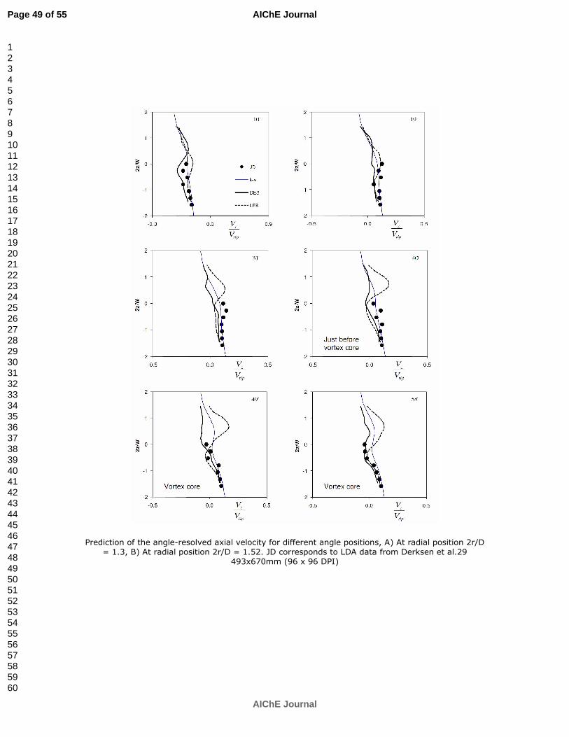
For peer review only
Prediction of the angle-resolved axial velocity for different angle positions, A) At radial position 2r/D = 1.3, B) At radial position 2r/D = 1.52. JD corresponds to LDA data from Derksen et al.29
493x670mm (96 x 96 DPI)
Page 49 of 55
AIChE Journal
AIChE Journal
123456789101112131415161718192021222324252627282930313233343536373839404142434445464748495051525354555657585960

For peer review only
Prediction of the angle-resolved turbulent kinetic energy for different angle positions, A) , at radial position 2r/D = 1.3, B) , at radial position 2r/D = 1.52. JD corresponds to LDA data from Derksen
et al.29 490x675mm (96 x 96 DPI)
Page 50 of 55
AIChE Journal
AIChE Journal
123456789101112131415161718192021222324252627282930313233343536373839404142434445464748495051525354555657585960

For peer review only
Prediction of the angle-resolved turbulent kinetic energy for different angle positions, A) , at radial position 2r/D = 1.3, B) , at radial position 2r/D = 1.52. JD corresponds to LDA data from Derksen
et al.29 496x684mm (96 x 96 DPI)
Page 51 of 55
AIChE Journal
AIChE Journal
123456789101112131415161718192021222324252627282930313233343536373839404142434445464748495051525354555657585960

For peer review only
Power spectrum from the DES at 2z/W = -1.57 using the instantaneous tangential velocity for N = 3.14 rev/s, A) DES 2r/D = 1.1, B) LES 2r/D = 1.1, C) DES 2r/D = 1.52, D) LES 2r/D = 1.52
243x187mm (96 x 96 DPI)
Page 52 of 55
AIChE Journal
AIChE Journal
123456789101112131415161718192021222324252627282930313233343536373839404142434445464748495051525354555657585960

For peer review only
Power spectrum from the DES at 2z/W = -1.57 using the instantaneous tangential velocity for N = 3.14 rev/s, A) DES 2r/D = 1.1, B) LES 2r/D = 1.1, C) DES 2r/D = 1.52, D) LES 2r/D = 1.52
243x185mm (96 x 96 DPI)
Page 53 of 55
AIChE Journal
AIChE Journal
123456789101112131415161718192021222324252627282930313233343536373839404142434445464748495051525354555657585960

For peer review only
Power spectrum from the DES at 2z/W = -1.57 using the instantaneous tangential velocity for N = 3.14 rev/s, A) DES 2r/D = 1.1, B) LES 2r/D = 1.1, C) DES 2r/D = 1.52, D) LES 2r/D = 1.52
243x188mm (96 x 96 DPI)
Page 54 of 55
AIChE Journal
AIChE Journal
123456789101112131415161718192021222324252627282930313233343536373839404142434445464748495051525354555657585960

For peer review only
Power spectrum from the DES at 2z/W = -1.57 using the instantaneous tangential velocity for N = 3.14 rev/s, A) DES 2r/D = 1.1, B) LES 2r/D = 1.1, C) DES 2r/D = 1.52, D) LES 2r/D = 1.52
243x185mm (96 x 96 DPI)
Page 55 of 55
AIChE Journal
AIChE Journal
123456789101112131415161718192021222324252627282930313233343536373839404142434445464748495051525354555657585960