


© 2008 Prentice Hall, Inc. 13 – 1
Operations ManagementChapter 13 – Chapter 13 – Aggregate PlanningAggregate Planning
PowerPoint presentation to accompany PowerPoint presentation to accompany Heizer/Render Heizer/Render Principles of Operations Management, 7ePrinciples of Operations Management, 7eOperations Management, 9e Operations Management, 9e
© 2008 Prentice Hall, Inc. 13 – 2
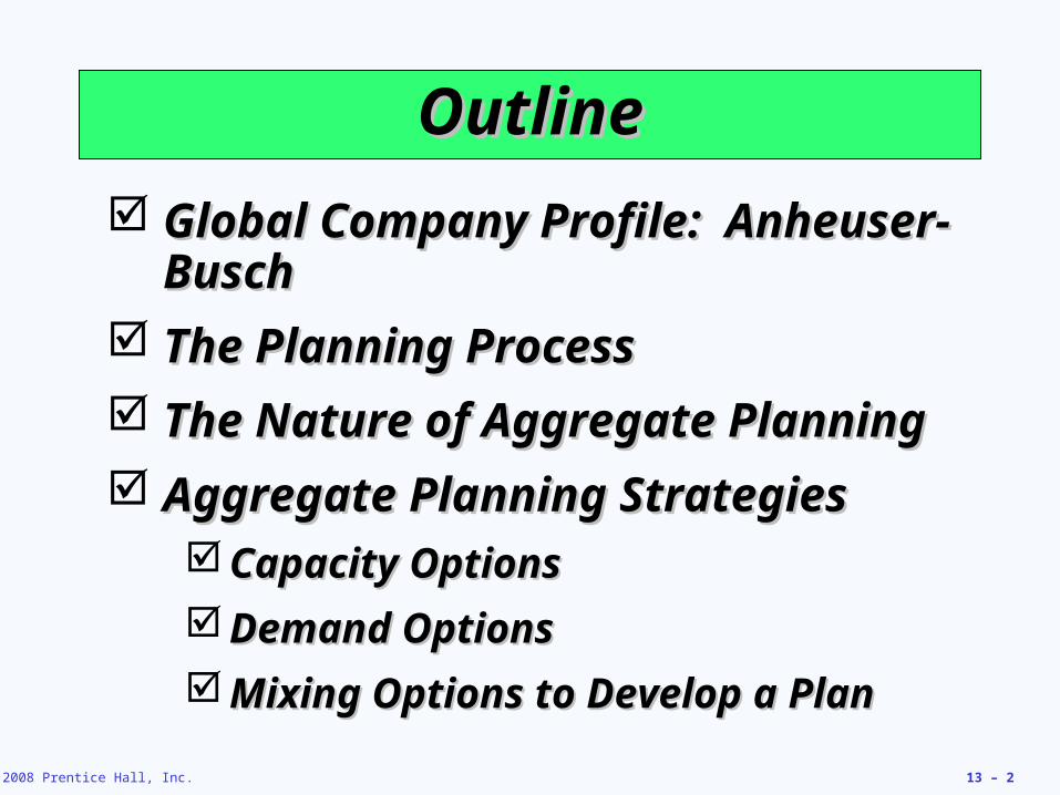
OutlineOutline Global Company Profile: Global Company Profile:
Anheuser-BuschAnheuser-Busch The Planning ProcessThe Planning Process The Nature of Aggregate PlanningThe Nature of Aggregate Planning Aggregate Planning StrategiesAggregate Planning Strategies
Capacity OptionsCapacity Options Demand OptionsDemand Options Mixing Options to Develop a PlanMixing Options to Develop a Plan
© 2008 Prentice Hall, Inc. 13 – 3
Outline – ContinuedOutline – Continued
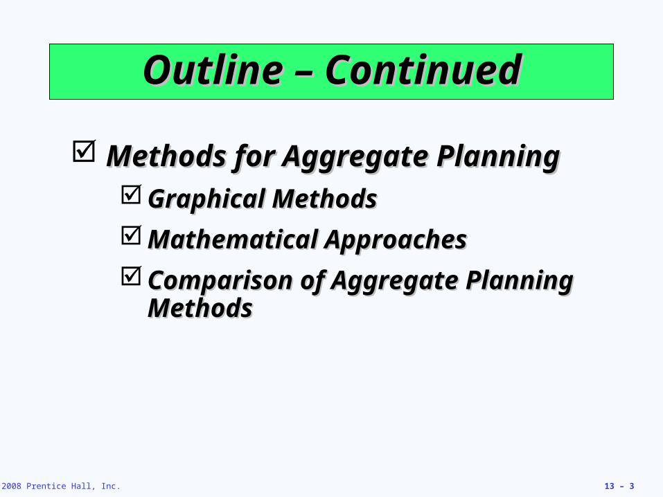
Methods for Aggregate PlanningMethods for Aggregate Planning Graphical MethodsGraphical Methods Mathematical ApproachesMathematical Approaches Comparison of Aggregate Planning Comparison of Aggregate Planning
MethodsMethods

© 2008 Prentice Hall, Inc. 13 – 4
Outline – ContinuedOutline – Continued Aggregate Planning in ServicesAggregate Planning in Services
RestaurantsRestaurants HospitalsHospitals National Chains of Small Service National Chains of Small Service
FirmsFirms Miscellaneous ServicesMiscellaneous Services
Airline IndustryAirline Industry Yield ManagementYield Management

© 2008 Prentice Hall, Inc. 13 – 5
Learning ObjectivesLearning ObjectivesWhen you complete this chapter you When you complete this chapter you should be able to:should be able to:
1.1. Define aggregate planningDefine aggregate planning2.2. Identify optional strategies for Identify optional strategies for
developing an aggregate plandeveloping an aggregate plan3.3. Prepare a graphical aggregate planPrepare a graphical aggregate plan

© 2008 Prentice Hall, Inc. 13 – 6
Learning ObjectivesLearning ObjectivesWhen you complete this chapter you When you complete this chapter you should be able to:should be able to:
4.4. Solve an aggregate plan via the Solve an aggregate plan via the transportation method of linear transportation method of linear programmingprogramming
5.5. Understand and solve a yield Understand and solve a yield management problemmanagement problem

© 2008 Prentice Hall, Inc. 13 – 7
Anheuser-BuschAnheuser-Busch
Anheuser-Busch produces nearly 40% Anheuser-Busch produces nearly 40% of the beer consumed in the U.S.of the beer consumed in the U.S.
Matches fluctuating demand by brand Matches fluctuating demand by brand to plant, labor, and inventory capacity to plant, labor, and inventory capacity to achieve high facility utilizationto achieve high facility utilization
High facility utilization requiresHigh facility utilization requires Meticulous cleaning between batchesMeticulous cleaning between batches Effective maintenanceEffective maintenance Efficient employee and facility schedulingEfficient employee and facility scheduling
© 2008 Prentice Hall, Inc. 13 – 8
Anheuser-BuschAnheuser-Busch
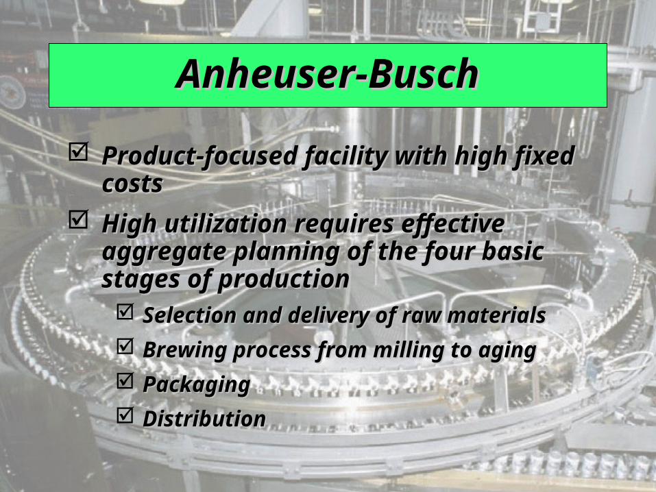
Product-focused facility with high fixed Product-focused facility with high fixed costscosts
High utilization requires effective High utilization requires effective aggregate planning of the four basic aggregate planning of the four basic stages of productionstages of production Selection and delivery of raw materialsSelection and delivery of raw materials Brewing process from milling to agingBrewing process from milling to aging PackagingPackaging DistributionDistribution
© 2008 Prentice Hall, Inc. 13 – 9
Aggregate PlanningAggregate Planning
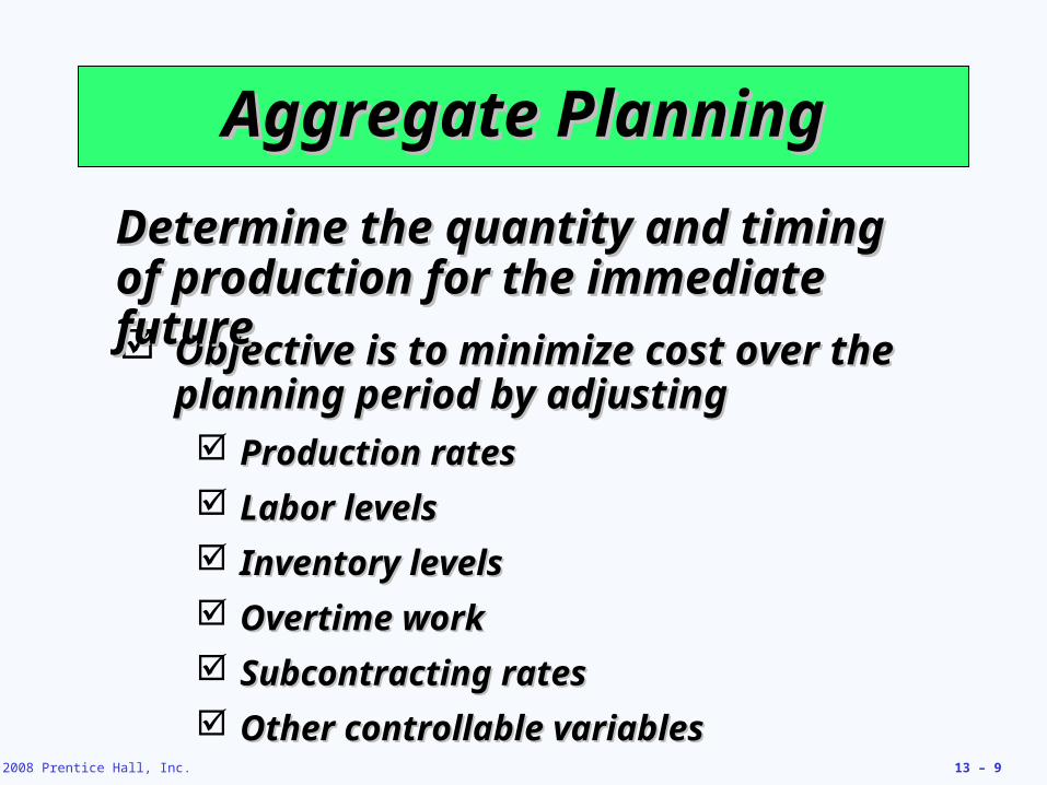
Objective is to minimize cost over the Objective is to minimize cost over the planning period by adjustingplanning period by adjusting Production ratesProduction rates Labor levelsLabor levels Inventory levelsInventory levels Overtime workOvertime work Subcontracting ratesSubcontracting rates Other controllable variablesOther controllable variables
Determine the quantity and timing of Determine the quantity and timing of production for the immediate futureproduction for the immediate future

© 2008 Prentice Hall, Inc. 13 – 10
Aggregate PlanningAggregate Planning
A logical overall unit for measuring sales A logical overall unit for measuring sales and outputand output
A forecast of demand for an intermediate A forecast of demand for an intermediate planning period in these aggregate termsplanning period in these aggregate terms
A method for determining costsA method for determining costs A model that combines forecasts and A model that combines forecasts and
costs so that scheduling decisions can costs so that scheduling decisions can be made for the planning periodbe made for the planning period
Required for aggregate planningRequired for aggregate planning
© 2008 Prentice Hall, Inc. 13 – 11
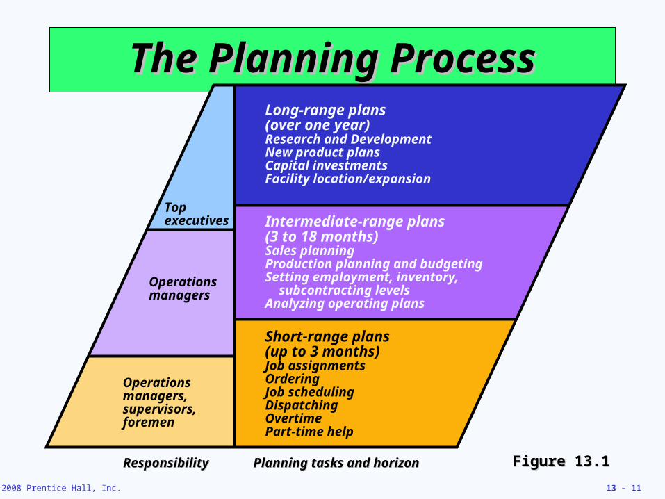
The Planning ProcessThe Planning Process
Figure 13.1Figure 13.1
Long-range plans (over one year)Research and DevelopmentNew product plansCapital investmentsFacility location/expansion
Intermediate-range plans (3 to 18 months)Sales planningProduction planning and budgetingSetting employment, inventory,
subcontracting levelsAnalyzing operating plans
Short-range plans (up to 3 months)Job assignmentsOrderingJob schedulingDispatchingOvertimePart-time help
Top executives
Operations managers
Operations managers, supervisors, foremen
ResponsibilityResponsibility Planning tasks and horizonPlanning tasks and horizon

© 2008 Prentice Hall, Inc. 13 – 12
Aggregate PlanningAggregate Planning
Quarter 1Quarter 1JanJan FebFeb MarMar
150,000150,000 120,000120,000 110,000110,000
Quarter 2Quarter 2AprApr MayMay JunJun
100,000100,000 130,000130,000 150,000150,000
Quarter 3Quarter 3JulJul AugAug SepSep
180,000180,000 150,000150,000 140,000140,000
© 2008 Prentice Hall, Inc. 13 – 13
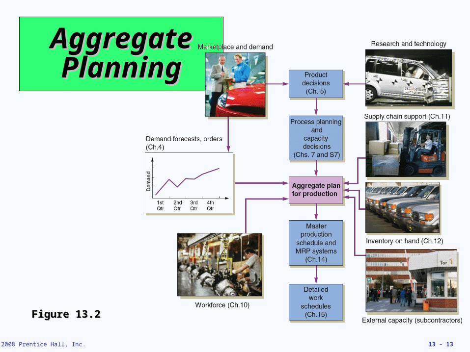
Aggregate Aggregate PlanningPlanning
Figure 13.2Figure 13.2
© 2008 Prentice Hall, Inc. 13 – 14
Aggregate PlanningAggregate Planning
Combines appropriate resources Combines appropriate resources into general termsinto general terms
Part of a larger production planning Part of a larger production planning systemsystem
Disaggregation breaks the plan Disaggregation breaks the plan down into greater detaildown into greater detail
Disaggregation results in a master Disaggregation results in a master production scheduleproduction schedule
© 2008 Prentice Hall, Inc. 13 – 15
Aggregate Planning Aggregate Planning StrategiesStrategies
1.1. Use inventories to absorb changes in Use inventories to absorb changes in demanddemand
2.2. Accommodate changes by varying Accommodate changes by varying workforce sizeworkforce size
3.3. Use part-timers, overtime, or idle time to Use part-timers, overtime, or idle time to absorb changesabsorb changes
4.4. Use subcontractors and maintain a stable Use subcontractors and maintain a stable workforceworkforce
5.5. Change prices or other factors to Change prices or other factors to influence demandinfluence demand
© 2008 Prentice Hall, Inc. 13 – 16
Capacity OptionsCapacity Options Changing inventory levelsChanging inventory levels
Increase inventory in low demand Increase inventory in low demand periods to meet high demand in periods to meet high demand in the futurethe future
Increases costs associated with Increases costs associated with storage, insurance, handling, storage, insurance, handling, obsolescence, and capital obsolescence, and capital investment 15% to 40%investment 15% to 40%
Shortages can mean lost sales due Shortages can mean lost sales due to long lead times and poor to long lead times and poor customer servicecustomer service
© 2008 Prentice Hall, Inc. 13 – 17
Capacity OptionsCapacity Options Varying workforce size by hiring Varying workforce size by hiring
or layoffsor layoffs Match production rate to demandMatch production rate to demand Training and separation costs for Training and separation costs for
hiring and laying off workers hiring and laying off workers New workers may have lower New workers may have lower
productivityproductivity Laying off workers may lower Laying off workers may lower
morale and productivitymorale and productivity

© 2008 Prentice Hall, Inc. 13 – 18
Capacity OptionsCapacity Options Varying production rate through Varying production rate through
overtime or idle timeovertime or idle time Allows constant workforceAllows constant workforce May be difficult to meet large May be difficult to meet large
increases in demandincreases in demand Overtime can be costly and may Overtime can be costly and may
drive down productivitydrive down productivity Absorbing idle time may be Absorbing idle time may be
difficultdifficult

© 2008 Prentice Hall, Inc. 13 – 19
Capacity OptionsCapacity Options SubcontractingSubcontracting
Temporary measure during Temporary measure during periods of peak demandperiods of peak demand
May be costlyMay be costly Assuring quality and timely Assuring quality and timely
delivery may be difficultdelivery may be difficult Exposes your customers to a Exposes your customers to a
possible competitorpossible competitor

© 2008 Prentice Hall, Inc. 13 – 20
Capacity OptionsCapacity Options Using part-time workersUsing part-time workers
Useful for filling unskilled or low Useful for filling unskilled or low skilled positions, especially in skilled positions, especially in servicesservices
© 2008 Prentice Hall, Inc. 13 – 21
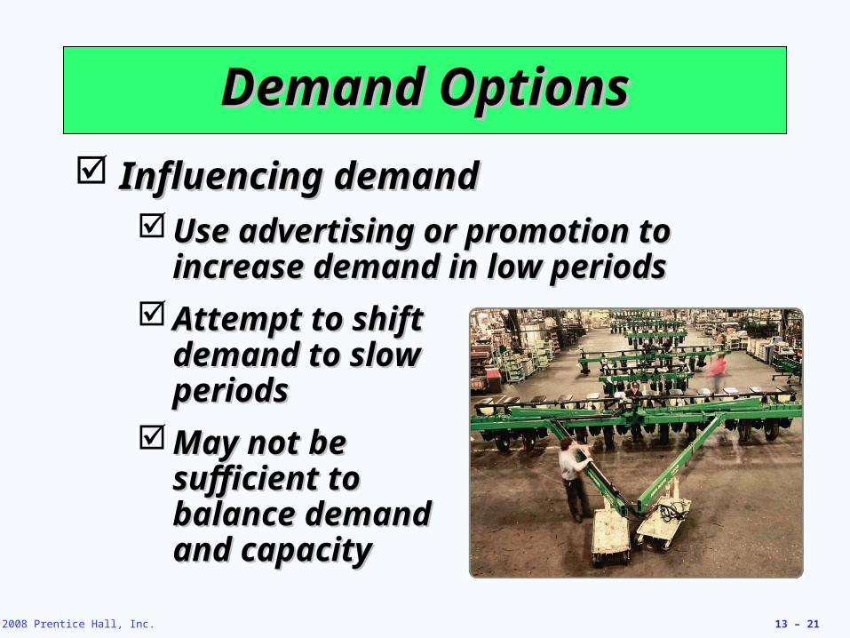
Demand OptionsDemand Options Influencing demandInfluencing demand
Use advertising or promotion to Use advertising or promotion to increase demand in low periodsincrease demand in low periods
Attempt to shift Attempt to shift demand to slow demand to slow periodsperiods
May not be May not be sufficient to sufficient to balance demand balance demand and capacityand capacity
© 2008 Prentice Hall, Inc. 13 – 22
Demand OptionsDemand Options Back ordering during high- Back ordering during high-
demand periodsdemand periods Requires customers to wait for an Requires customers to wait for an
order without loss of goodwill or order without loss of goodwill or the orderthe order
Most effective when there are few Most effective when there are few if any substitutes for the product if any substitutes for the product or serviceor service
Often results in lost salesOften results in lost sales

© 2008 Prentice Hall, Inc. 13 – 23
Demand OptionsDemand Options Counterseasonal product and Counterseasonal product and
service mixingservice mixing Develop a product mix of Develop a product mix of
counterseasonal itemscounterseasonal items May lead to products or services May lead to products or services
outside the company’s areas of outside the company’s areas of expertiseexpertise

© 2008 Prentice Hall, Inc. 13 – 24
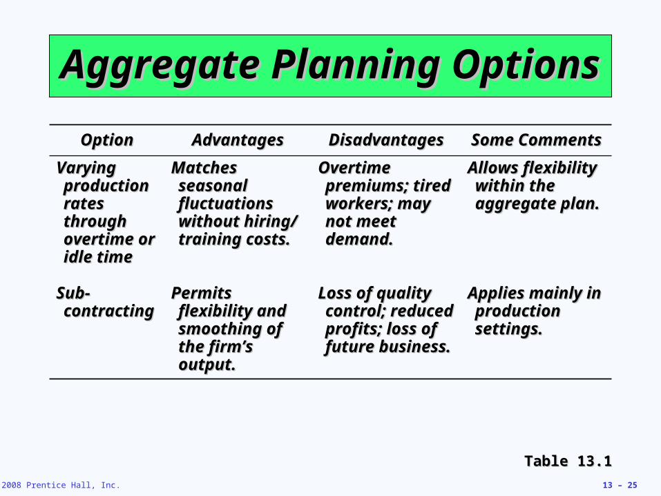
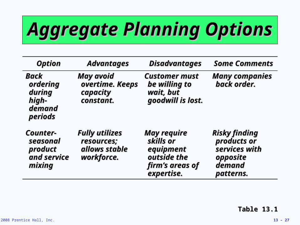
Aggregate Planning OptionsAggregate Planning Options
Table 13.1Table 13.1
OptionOption AdvantagesAdvantages DisadvantagesDisadvantages Some CommentsSome CommentsChanging Changing inventory inventory levelslevels
Changes in Changes in human human resources are resources are gradual or gradual or none; no abrupt none; no abrupt production production changes.changes.
Inventory Inventory holding cost holding cost may increase. may increase. Shortages may Shortages may result in lost result in lost sales.sales.
Applies mainly to Applies mainly to production, not production, not service, service, operations.operations.
Varying Varying workforce workforce size by size by hiring or hiring or layoffslayoffs
Avoids the costs Avoids the costs of other of other alternatives.alternatives.
Hiring, layoff, Hiring, layoff, and training and training costs may be costs may be significant.significant.
Used where size Used where size of labor pool is of labor pool is large.large.
© 2008 Prentice Hall, Inc. 13 – 25
Aggregate Planning OptionsAggregate Planning Options
Table 13.1Table 13.1
OptionOption AdvantagesAdvantages DisadvantagesDisadvantages Some CommentsSome CommentsVarying Varying production production rates rates through through overtime or overtime or idle timeidle time
Matches Matches seasonal seasonal fluctuations fluctuations without hiring/ without hiring/ training costs.training costs.
Overtime Overtime premiums; tired premiums; tired workers; may workers; may not meet not meet demand.demand.
Allows flexibility Allows flexibility within the within the aggregate plan.aggregate plan.
Sub-Sub-contractingcontracting
Permits Permits flexibility and flexibility and smoothing of smoothing of the firm’s the firm’s output.output.
Loss of quality Loss of quality control; control; reduced profits; reduced profits; loss of future loss of future business.business.
Applies mainly in Applies mainly in production production settings.settings.

© 2008 Prentice Hall, Inc. 13 – 26
Aggregate Planning OptionsAggregate Planning Options
Table 13.1Table 13.1
OptionOption AdvantagesAdvantages DisadvantagesDisadvantages Some CommentsSome CommentsUsing part-Using part-time time workersworkers
Is less costly Is less costly and more and more flexible than flexible than full-time full-time workers.workers.
High turnover/ High turnover/ training costs; training costs; quality suffers; quality suffers; scheduling scheduling difficult.difficult.
Good for Good for unskilled jobs in unskilled jobs in areas with large areas with large temporary labor temporary labor pools.pools.
Influencing Influencing demanddemand
Tries to use Tries to use excess excess capacity. capacity. Discounts draw Discounts draw new customers.new customers.
Uncertainty in Uncertainty in demand. Hard demand. Hard to match to match demand to demand to supply exactly.supply exactly.
Creates Creates marketing marketing ideas. ideas. Overbooking Overbooking used in some used in some businesses.businesses.
© 2008 Prentice Hall, Inc. 13 – 27
Aggregate Planning OptionsAggregate Planning Options
Table 13.1Table 13.1
OptionOption AdvantagesAdvantages DisadvantagesDisadvantages Some CommentsSome CommentsBack Back ordering ordering during during high-high-demand demand periodsperiods
May avoid May avoid overtime. overtime. Keeps capacity Keeps capacity constant.constant.
Customer must Customer must be willing to be willing to wait, but wait, but goodwill is lost.goodwill is lost.
Many companies Many companies back order.back order.
Counter-Counter-seasonal seasonal product product and service and service mixingmixing
Fully utilizes Fully utilizes resources; resources; allows stable allows stable workforce.workforce.
May require May require skills or skills or equipment equipment outside the outside the firm’s areas of firm’s areas of expertise.expertise.
Risky finding Risky finding products or products or services with services with opposite opposite demand demand patterns.patterns.
© 2008 Prentice Hall, Inc. 13 – 28
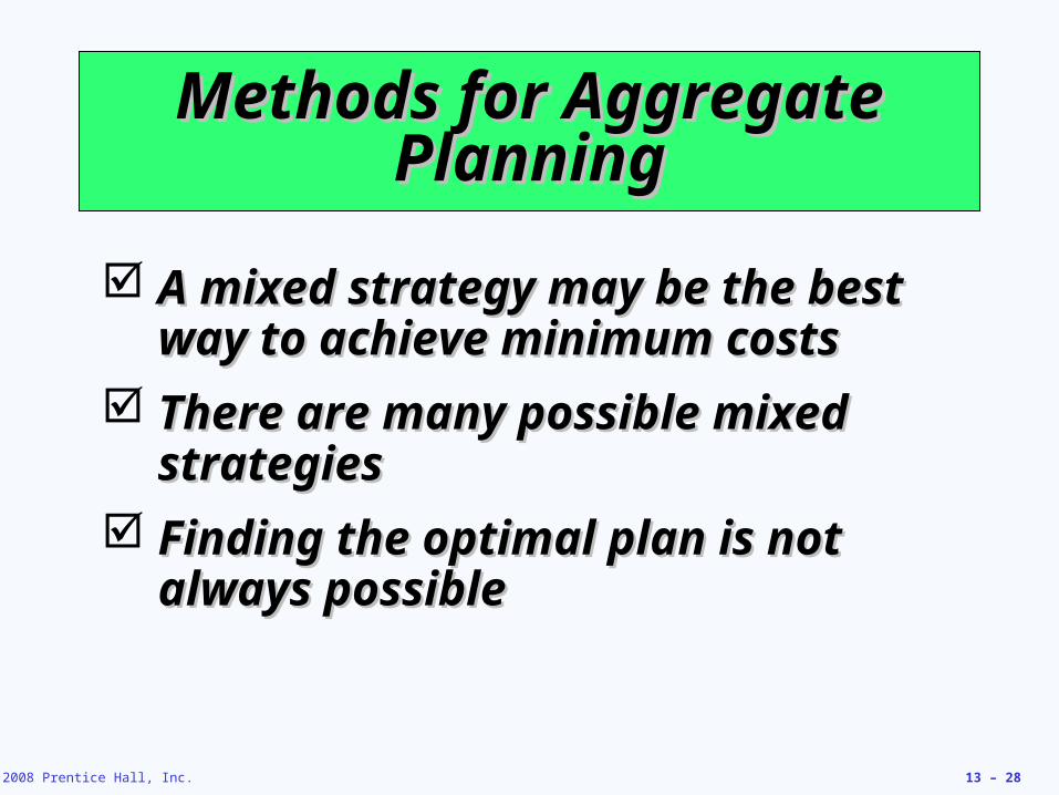
Methods for Aggregate Methods for Aggregate PlanningPlanning
A mixed strategy may be the best A mixed strategy may be the best way to achieve minimum costsway to achieve minimum costs
There are many possible mixed There are many possible mixed strategiesstrategies
Finding the optimal plan is not Finding the optimal plan is not always possiblealways possible
© 2008 Prentice Hall, Inc. 13 – 29
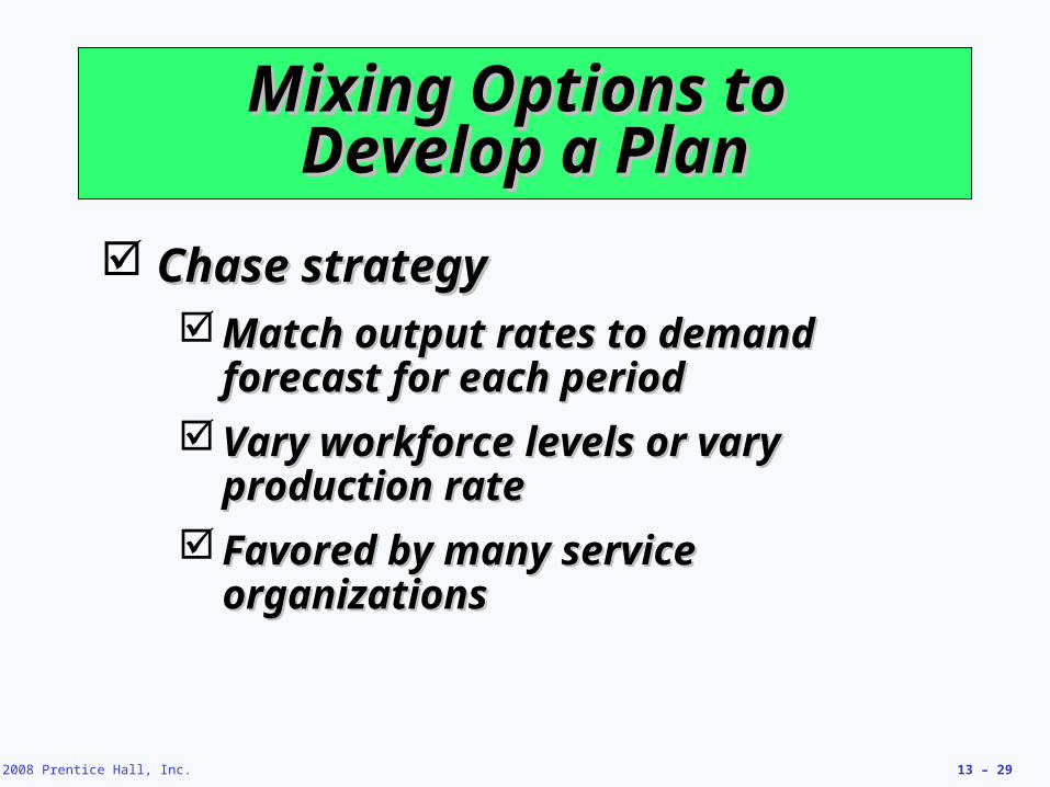
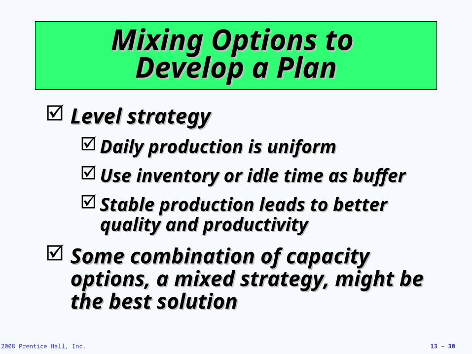
Mixing Options to Mixing Options to Develop a PlanDevelop a Plan
Chase strategyChase strategy Match output rates to demand Match output rates to demand
forecast for each periodforecast for each period Vary workforce levels or vary Vary workforce levels or vary
production rateproduction rate Favored by many service Favored by many service
organizationsorganizations
© 2008 Prentice Hall, Inc. 13 – 30
Mixing Options to Mixing Options to Develop a PlanDevelop a Plan
Level strategyLevel strategy Daily production is uniformDaily production is uniform Use inventory or idle time as bufferUse inventory or idle time as buffer Stable production leads to better Stable production leads to better
quality and productivityquality and productivity Some combination of capacity Some combination of capacity
options, a mixed strategy, might be options, a mixed strategy, might be the best solutionthe best solution

© 2008 Prentice Hall, Inc. 13 – 31
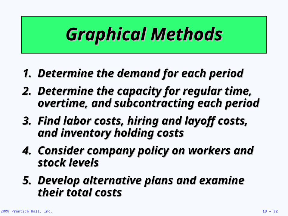
Graphical MethodsGraphical Methods
Popular techniquesPopular techniques Easy to understand and useEasy to understand and use Trial-and-error approaches that do Trial-and-error approaches that do
not guarantee an optimal solutionnot guarantee an optimal solution Require only limited computationsRequire only limited computations
© 2008 Prentice Hall, Inc. 13 – 32
Graphical MethodsGraphical Methods
1.1. Determine the demand for each periodDetermine the demand for each period2.2. Determine the capacity for regular time, Determine the capacity for regular time,
overtime, and subcontracting each periodovertime, and subcontracting each period3.3. Find labor costs, hiring and layoff costs, Find labor costs, hiring and layoff costs,
and inventory holding costsand inventory holding costs4.4. Consider company policy on workers and Consider company policy on workers and
stock levelsstock levels5.5. Develop alternative plans and examine Develop alternative plans and examine
their total coststheir total costs

© 2008 Prentice Hall, Inc. 13 – 33
Roofing Supplier Example 1Roofing Supplier Example 1
Table 13.2Table 13.2
MonthMonth Expected DemandExpected DemandProduction Production
DaysDaysDemand Per Day Demand Per Day
(computed)(computed)JanJan 900900 2222 4141FebFeb 700700 1818 3939MarMar 800800 2121 3838AprApr 1,2001,200 2121 5757MayMay 1,5001,500 2222 6868JuneJune 1,1001,100 2020 5555
6,2006,200 124124
= = 50= = 50 units per day units per day6,2006,200124124
Average Average requirementrequirement == Total expected demandTotal expected demand
Number of production daysNumber of production days
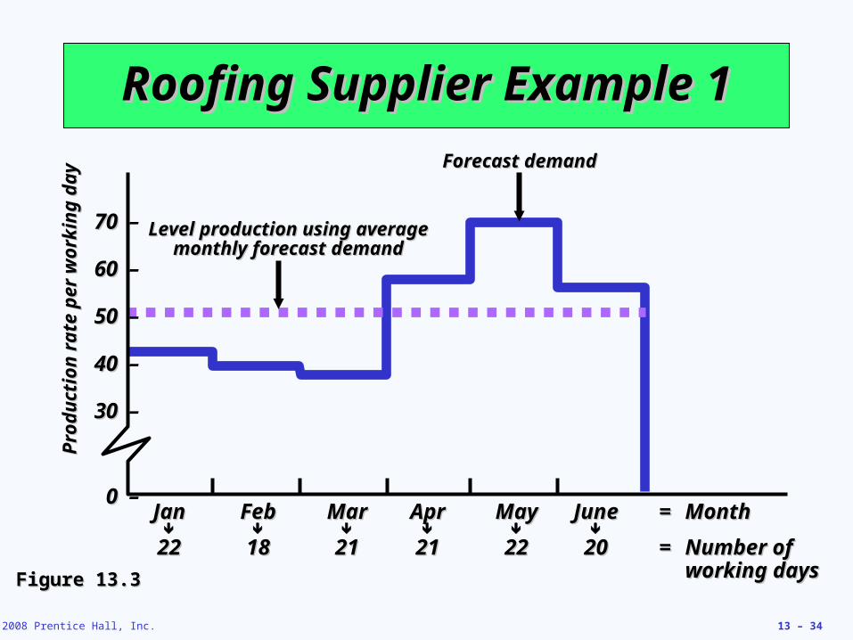
© 2008 Prentice Hall, Inc. 13 – 34
Roofing Supplier Example 1Roofing Supplier Example 1
Figure 13.3Figure 13.3
70 70 –
60 60 –
50 50 –
40 40 –
30 30 –
0 0 –JanJan FebFeb MarMar AprApr MayMay JuneJune == MonthMonth
2222 1818 2121 2121 2222 2020 == Number ofNumber ofworking daysworking days
Prod
uctio
n ra
te p
er w
orki
ng d
ayPr
oduc
tion
rate
per
wor
king
day
Level production using average Level production using average monthly forecast demandmonthly forecast demand
Forecast demandForecast demand

© 2008 Prentice Hall, Inc. 13 – 35
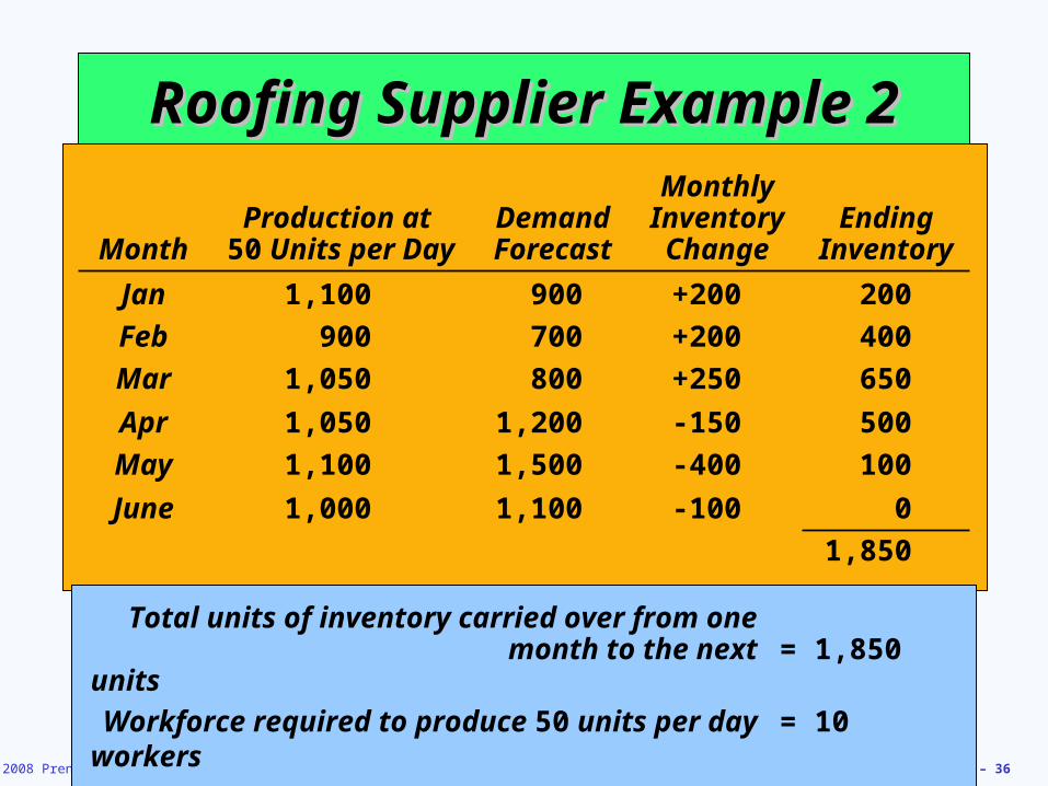
Roofing Supplier Example 2Roofing Supplier Example 2
Table 13.3Table 13.3
Cost InformationCost InformationInventory carrying costInventory carrying cost $ 5$ 5 per unit per month per unit per monthSubcontracting cost per unitSubcontracting cost per unit $10$10 per unit per unit
Average pay rateAverage pay rate $ 5$ 5 per hour per hour ($40($40 per day per day))
Overtime pay rateOvertime pay rate $ 7$ 7 per hour per hour ((above above 88 hours per day hours per day))
Labor-hours to produce a unitLabor-hours to produce a unit 1.61.6 hours per unit hours per unit
Cost of increasing daily production rate Cost of increasing daily production rate (hiring and training)(hiring and training)
$300$300 per unit per unit
Cost of decreasing daily production rate Cost of decreasing daily production rate (layoffs)(layoffs)
$600$600 per unit per unit
Plan 1 – constant workforce
Plan 1 – constant workforce
© 2008 Prentice Hall, Inc. 13 – 36
Roofing Supplier Example 2Roofing Supplier Example 2
Table 13.3Table 13.3
Cost InformationCost InformationInventory carry costInventory carry cost $ 5$ 5 per unit per month per unit per monthSubcontracting cost per unitSubcontracting cost per unit $10$10 per unit per unit
Average pay rateAverage pay rate $ 5$ 5 per hour per hour ($40($40 per day per day))
Overtime pay rateOvertime pay rate $ 7$ 7 per hour per hour ((above above 88 hours per day hours per day))
Labor-hours to produce a unitLabor-hours to produce a unit 1.61.6 hours per unit hours per unit
Cost of increasing daily production rate Cost of increasing daily production rate (hiring and training)(hiring and training)
$300$300 per unit per unit
Cost of decreasing daily production rate Cost of decreasing daily production rate (layoffs)(layoffs)
$600$600 per unit per unit
Plan 1 – constant workforce
Plan 1 – constant workforce
MonthProduction at
50 Units per DayDemand Forecast
Monthly Inventory Change
Ending Inventory
Jan 1,100 900 +200 200Feb 900 700 +200 400Mar 1,050 800 +250 650Apr 1,050 1,200 -150 500May 1,100 1,500 -400 100June 1,000 1,100 -100 0
1,850
Total units of inventory carried over from onemonth to the next = 1,850 units
Workforce required to produce 50 units per day = 10 workers

© 2008 Prentice Hall, Inc. 13 – 37
Roofing Supplier Example 2Roofing Supplier Example 2
Table 13.3Table 13.3
Cost InformationCost InformationInventory carry costInventory carry cost $ 5$ 5 per unit per month per unit per monthSubcontracting cost per unitSubcontracting cost per unit $10$10 per unit per unit
Average pay rateAverage pay rate $ 5$ 5 per hour per hour ($40($40 per day per day))
Overtime pay rateOvertime pay rate $ 7$ 7 per hour per hour ((above above 88 hours per day hours per day))
Labor-hours to produce a unitLabor-hours to produce a unit 1.61.6 hours per unit hours per unit
Cost of increasing daily production rate Cost of increasing daily production rate (hiring and training)(hiring and training)
$300$300 per unit per unit
Cost of decreasing daily production rate Cost of decreasing daily production rate (layoffs)(layoffs)
$600$600 per unit per unit
MonthProduction at
50 Units per DayDemand Forecast
Monthly Inventory Change
Ending Inventory
Jan 1,100 900 +200 200Feb 900 700 +200 400Mar 1,050 800 +250 650Apr 1,050 1,200 -150 500May 1,100 1,500 -400 100June 1,000 1,100 -100 0
1,850
Total units of inventory carried over from onemonth to the next = 1,850 units
Workforce required to produce 50 units per day = 10 workers
Costs CalculationsInventory carrying $9,250 (= 1,850 units carried x $5
per unit)Regular-time labor 49,600 (= 10 workers x $40 per
day x 124 days)Other costs (overtime,
hiring, layoffs, subcontracting) 0
Total cost $58,850

© 2008 Prentice Hall, Inc. 13 – 38
Roofing Supplier Example 2Roofing Supplier Example 2
Figure 13.4Figure 13.4
Cum
ulat
ive
dem
and
units
Cum
ulat
ive
dem
and
units
7,000 7,000 –
6,000 6,000 –
5,000 5,000 –
4,000 4,000 –
3,000 3,000 –
2,000 –
1,000 –
–JanJan FebFeb MarMar AprApr MayMay JuneJune
Cumulative forecast Cumulative forecast requirementsrequirements
Cumulative level Cumulative level production using production using average monthly average monthly
forecast forecast requirementsrequirements
Reduction Reduction of inventoryof inventory
Excess inventoryExcess inventory
6,200 units6,200 units
© 2008 Prentice Hall, Inc. 13 – 39
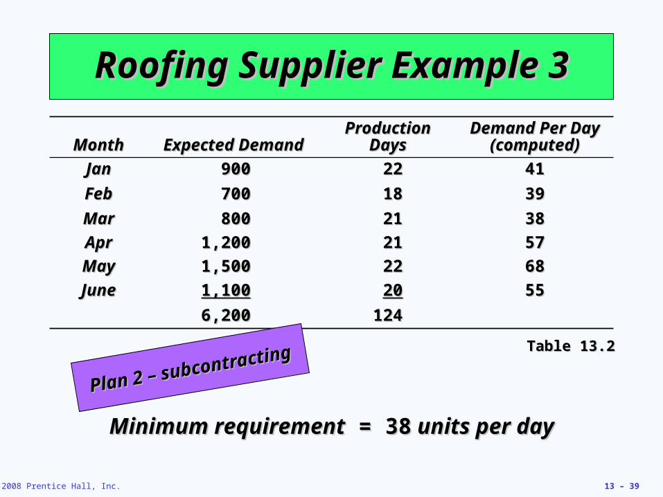
Roofing Supplier Example 3Roofing Supplier Example 3
Table 13.2Table 13.2
MonthMonth Expected DemandExpected DemandProduction Production
DaysDaysDemand Per Day Demand Per Day
(computed)(computed)JanJan 900900 2222 4141FebFeb 700700 1818 3939MarMar 800800 2121 3838AprApr 1,2001,200 2121 5757MayMay 1,5001,500 2222 6868JuneJune 1,1001,100 2020 5555
6,2006,200 124124
Minimum requirementMinimum requirement = 38 = 38 units per day units per day
Plan 2 – subcontractingPlan 2 – subcontracting

© 2008 Prentice Hall, Inc. 13 – 40
Roofing Supplier Example 3Roofing Supplier Example 3
70 70 –
60 60 –
50 50 –
40 40 –
30 30 –
0 0 –JanJan FebFeb MarMar AprApr MayMay JuneJune == MonthMonth
2222 1818 2121 2121 2222 2020 == Number ofNumber ofworking daysworking days
Prod
uctio
n ra
te p
er w
orki
ng d
ayPr
oduc
tion
rate
per
wor
king
day
Level production Level production using lowest using lowest
monthly forecast monthly forecast demanddemand
Forecast demandForecast demand
© 2008 Prentice Hall, Inc. 13 – 41
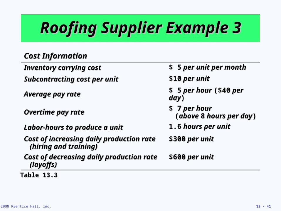
Roofing Supplier Example 3Roofing Supplier Example 3
Table 13.3Table 13.3
Cost InformationCost InformationInventory carrying costInventory carrying cost $ 5$ 5 per unit per month per unit per monthSubcontracting cost per unitSubcontracting cost per unit $10$10 per unit per unit
Average pay rateAverage pay rate $ 5$ 5 per hour per hour ($40($40 per day per day))
Overtime pay rateOvertime pay rate $ 7$ 7 per hour per hour ((above above 88 hours per day hours per day))
Labor-hours to produce a unitLabor-hours to produce a unit 1.61.6 hours per unit hours per unit
Cost of increasing daily production rate Cost of increasing daily production rate (hiring and training)(hiring and training)
$300$300 per unit per unit
Cost of decreasing daily production rate Cost of decreasing daily production rate (layoffs)(layoffs)
$600$600 per unit per unit

© 2008 Prentice Hall, Inc. 13 – 42
Roofing Supplier Example 3Roofing Supplier Example 3
Table 13.3Table 13.3
Cost InformationCost InformationInventory carry costInventory carry cost $ 5$ 5 per unit per month per unit per monthSubcontracting cost per unitSubcontracting cost per unit $10$10 per unit per unit
Average pay rateAverage pay rate $ 5$ 5 per hour per hour ($40($40 per day per day))
Overtime pay rateOvertime pay rate $ 7$ 7 per hour per hour ((above above 88 hours per day hours per day))
Labor-hours to produce a unitLabor-hours to produce a unit 1.61.6 hours per unit hours per unit
Cost of increasing daily production rate Cost of increasing daily production rate (hiring and training)(hiring and training)
$300$300 per unit per unit
Cost of decreasing daily production rate Cost of decreasing daily production rate (layoffs)(layoffs)
$600$600 per unit per unit
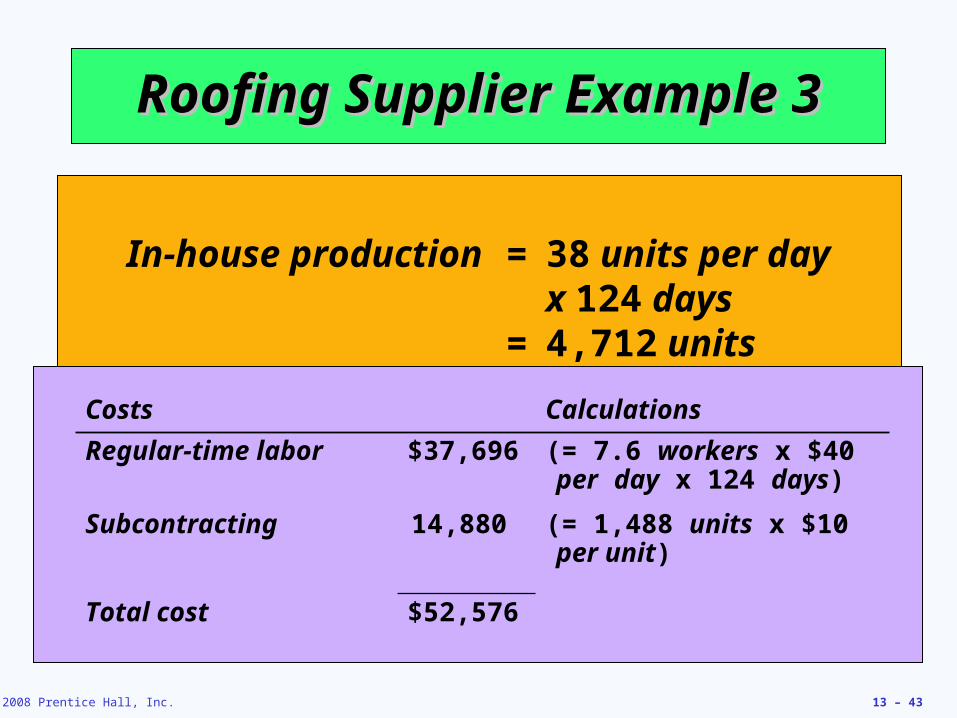
In-house production = 38 units per day x 124 days
= 4,712 units
Subcontract units = 6,200 - 4,712= 1,488 units
© 2008 Prentice Hall, Inc. 13 – 43
Table 13.3Table 13.3
Cost InformationCost InformationInventory carry costInventory carry cost $ 5$ 5 per unit per month per unit per monthSubcontracting cost per unitSubcontracting cost per unit $10$10 per unit per unit
Average pay rateAverage pay rate $ 5$ 5 per hour per hour ($40($40 per day per day))
Overtime pay rateOvertime pay rate $ 7$ 7 per hour per hour ((above above 88 hours per day hours per day))
Labor-hours to produce a unitLabor-hours to produce a unit 1.61.6 hours per unit hours per unit
Cost of increasing daily production rate Cost of increasing daily production rate (hiring and training)(hiring and training)
$300$300 per unit per unit
Cost of decreasing daily production rate Cost of decreasing daily production rate (layoffs)(layoffs)
$600$600 per unit per unit
Roofing Supplier Example 3Roofing Supplier Example 3
In-house production = 38 units per day x 124 days
= 4,712 units
Subcontract units = 6,200 - 4,712= 1,488 units
Costs CalculationsRegular-time labor $37,696 (= 7.6 workers x $40 per
day x 124 days)Subcontracting 14,880 (= 1,488 units x $10 per
unit)
Total cost $52,576

© 2008 Prentice Hall, Inc. 13 – 44
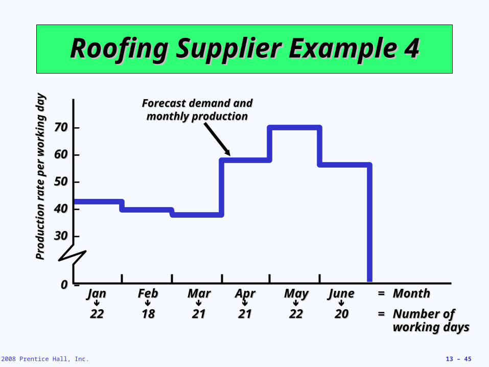
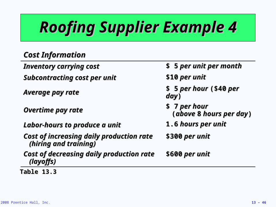
Roofing Supplier Example 4Roofing Supplier Example 4
Table 13.2Table 13.2
MonthMonth Expected DemandExpected DemandProduction Production
DaysDaysDemand Per Day Demand Per Day
(computed)(computed)JanJan 900900 2222 4141FebFeb 700700 1818 3939MarMar 800800 2121 3838AprApr 1,2001,200 2121 5757MayMay 1,5001,500 2222 6868JuneJune 1,1001,100 2020 5555
6,2006,200 124124
Production = Expected DemandProduction = Expected DemandPlan 3 – hiring and firing
Plan 3 – hiring and firing
© 2008 Prentice Hall, Inc. 13 – 45
Roofing Supplier Example 4Roofing Supplier Example 4
70 70 –
60 60 –
50 50 –
40 40 –
30 30 –
0 0 –JanJan FebFeb MarMar AprApr MayMay JuneJune == MonthMonth
2222 1818 2121 2121 2222 2020 == Number ofNumber ofworking daysworking days
Prod
uctio
n ra
te p
er w
orki
ng d
ayPr
oduc
tion
rate
per
wor
king
day Forecast demand and Forecast demand and
monthly productionmonthly production
© 2008 Prentice Hall, Inc. 13 – 46
Roofing Supplier Example 4Roofing Supplier Example 4
Table 13.3Table 13.3
Cost InformationCost InformationInventory carrying costInventory carrying cost $ 5$ 5 per unit per month per unit per monthSubcontracting cost per unitSubcontracting cost per unit $10$10 per unit per unit
Average pay rateAverage pay rate $ 5$ 5 per hour per hour ($40($40 per day per day))
Overtime pay rateOvertime pay rate $ 7$ 7 per hour per hour ((above above 88 hours per day hours per day))
Labor-hours to produce a unitLabor-hours to produce a unit 1.61.6 hours per unit hours per unit
Cost of increasing daily production rate Cost of increasing daily production rate (hiring and training)(hiring and training)
$300$300 per unit per unit
Cost of decreasing daily production rate Cost of decreasing daily production rate (layoffs)(layoffs)
$600$600 per unit per unit

© 2008 Prentice Hall, Inc. 13 – 47
Roofing Supplier Example 4Roofing Supplier Example 4
Table 13.3Table 13.3
Cost InformationCost InformationInventory carrying costInventory carrying cost $ 5$ 5 per unit per month per unit per monthSubcontracting cost per unitSubcontracting cost per unit $10$10 per unit per unit
Average pay rateAverage pay rate $ 5$ 5 per hour per hour ($40($40 per day per day))
Overtime pay rateOvertime pay rate $ 7$ 7 per hour per hour ((above above 88 hours per day hours per day))
Labor-hours to produce a unitLabor-hours to produce a unit 1.61.6 hours per unit hours per unit
Cost of increasing daily production rate Cost of increasing daily production rate (hiring and training)(hiring and training)
$300$300 per unit per unit
Cost of decreasing daily production rate Cost of decreasing daily production rate (layoffs)(layoffs)
$600$600 per unit per unit
MonthForecast
(units)
Daily Prod Rate
Basic Production
Cost (demand x
1.6 hrs/unit x $5/hr)
Extra Cost of Increasing Production (hiring cost)
Extra Cost of Decreasing Production (layoff cost) Total Cost
Jan 900 41 $ 7,200 — — $ 7,200
Feb 700 39 5,600 — $1,200 (= 2 x $600) 6,800
Mar 800 38 6,400 — $600 (= 1 x $600) 7,000
Apr 1,200 57 9,600 $5,700 (= 19 x $300) — 15,300
May 1,500 68 12,000 $3,300 (= 11 x $300) — 15,300
June 1,100 55 8,800 — $7,800 (= 13 x $600) 16,600
$49,600 $9,000 $9,600 $68,200
Table 13.4Table 13.4

© 2008 Prentice Hall, Inc. 13 – 48
Comparison of Three PlansComparison of Three Plans
Table 13.5Table 13.5
CostCost Plan 1Plan 1 Plan 2Plan 2 Plan 3Plan 3
Inventory carryingInventory carrying $ 9,250$ 9,250 $ 0$ 0 $ 0$ 0
Regular laborRegular labor 49,60049,600 37,69637,696 49,60049,600Overtime laborOvertime labor 00 00 00HiringHiring 00 00 9,0009,000LayoffsLayoffs 00 00 9,6009,600SubcontractingSubcontracting 00 14,88014,880 00Total costTotal cost $58,850$58,850 $52,576$52,576 $68,200$68,200
Plan 2 is the lowest cost optionPlan 2 is the lowest cost option
© 2008 Prentice Hall, Inc. 13 – 49
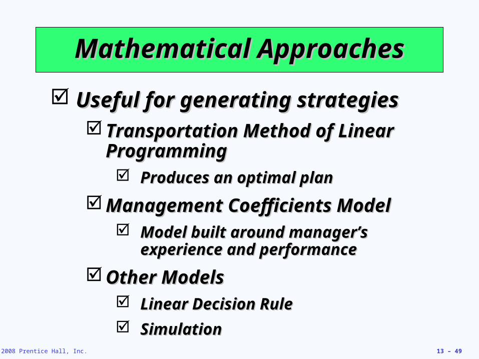
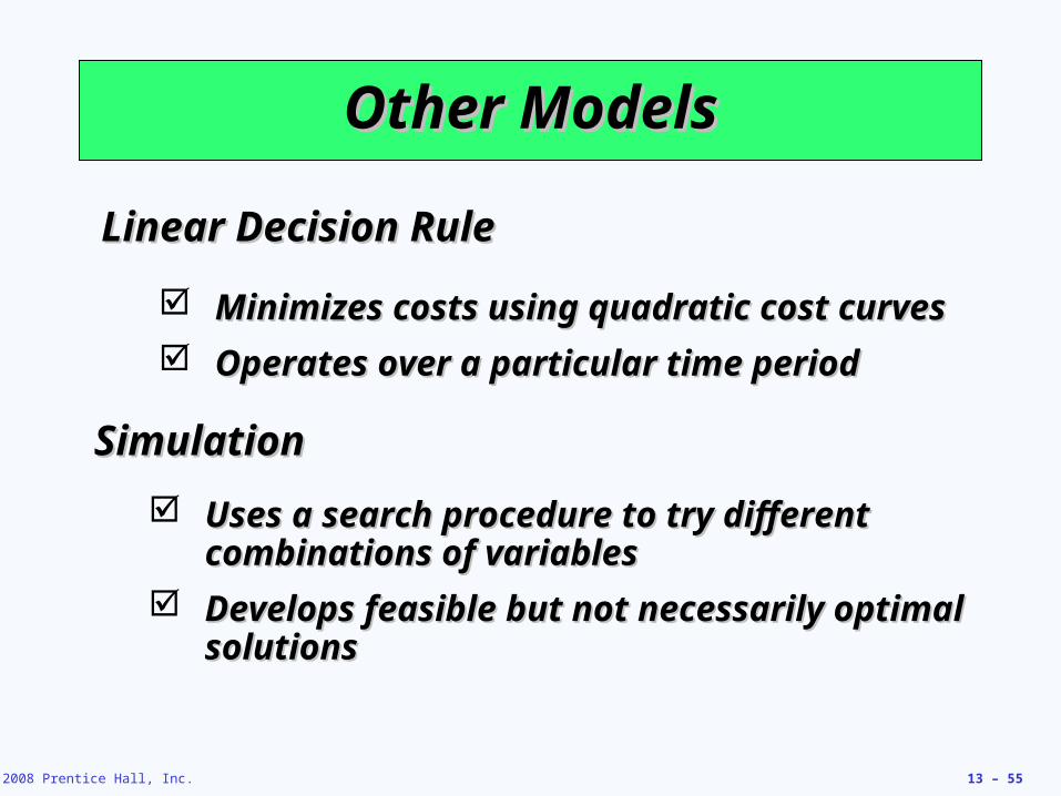
Mathematical ApproachesMathematical Approaches Useful for generating strategiesUseful for generating strategies
Transportation Method of Linear Transportation Method of Linear ProgrammingProgramming Produces an optimal planProduces an optimal plan
Management Coefficients ModelManagement Coefficients Model Model built around manager’s Model built around manager’s
experience and performanceexperience and performance Other ModelsOther Models
Linear Decision RuleLinear Decision Rule SimulationSimulation
© 2008 Prentice Hall, Inc. 13 – 50
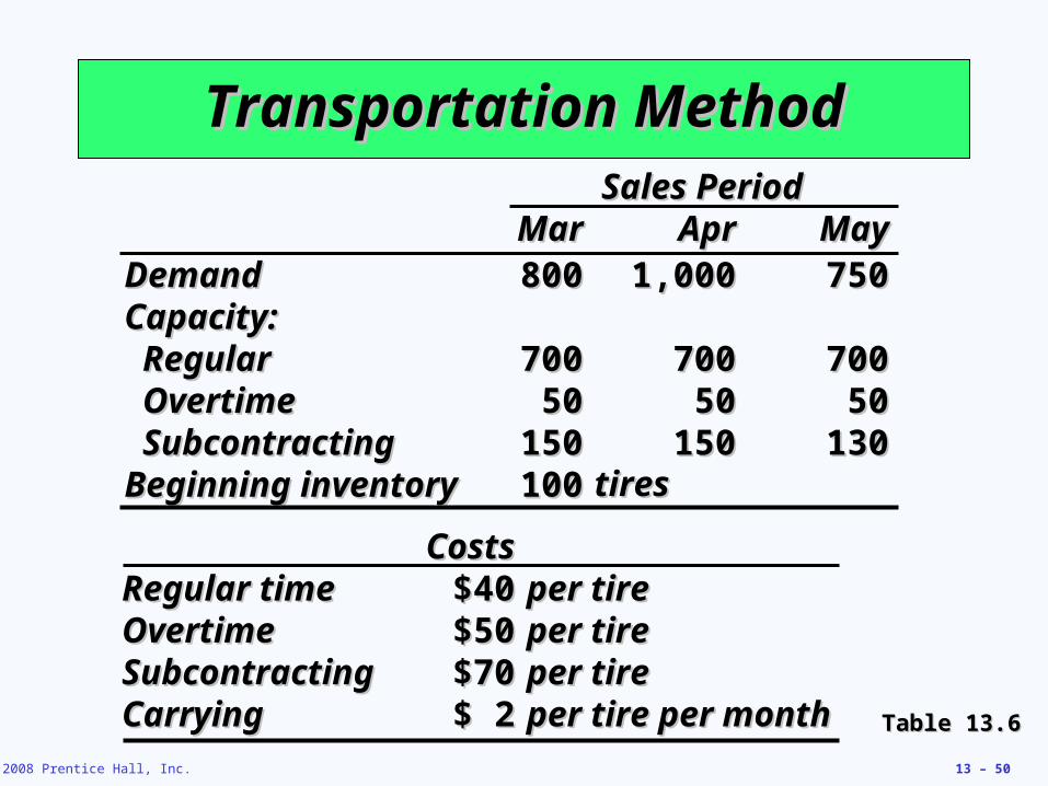
Transportation MethodTransportation Method
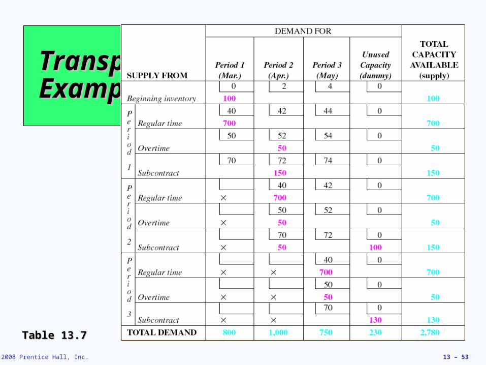
Table 13.6Table 13.6
CostsCostsRegular timeRegular time $40$40 per tireper tireOvertimeOvertime $50$50 per tireper tireSubcontractingSubcontracting $70$70 per tireper tireCarryingCarrying $ 2$ 2 per tire per monthper tire per month
Sales PeriodSales PeriodMarMar AprApr MayMay
DemandDemand 800800 1,0001,000 750750Capacity:Capacity: RegularRegular 700700 700700 700700 OvertimeOvertime 5050 5050 5050 SubcontractingSubcontracting 150150 150150 130130Beginning inventoryBeginning inventory 100100 tirestires
© 2008 Prentice Hall, Inc. 13 – 51
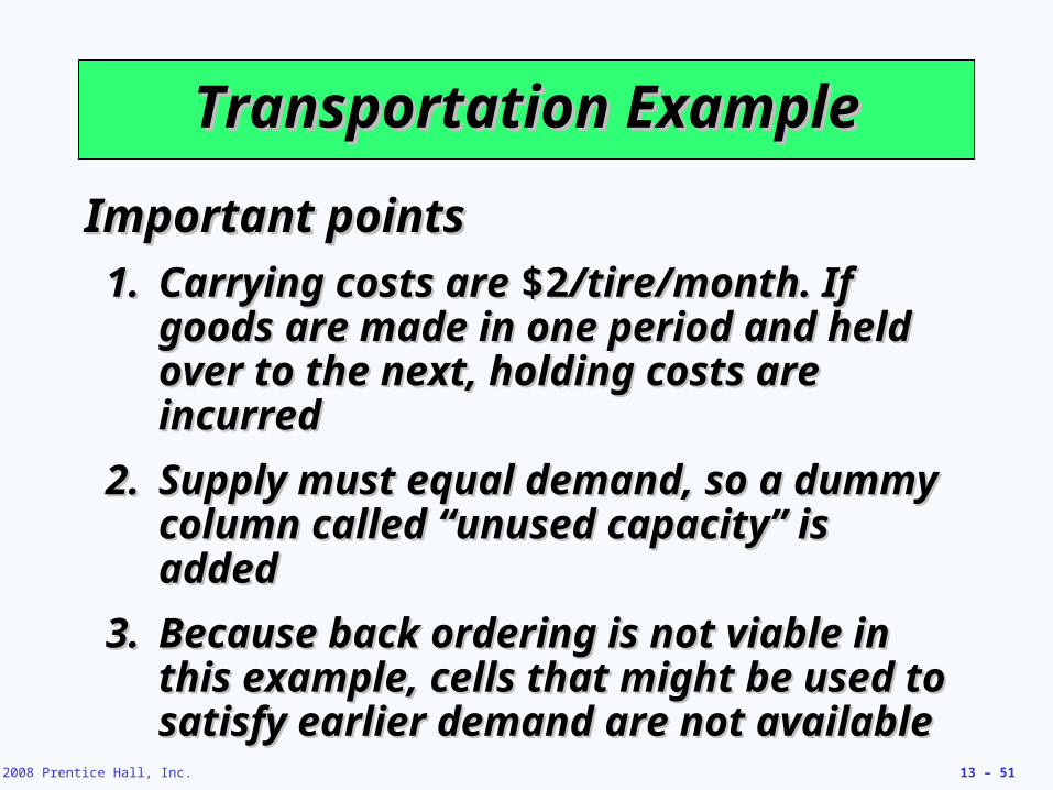
Transportation ExampleTransportation Example
Important pointsImportant points1.1. Carrying costs are Carrying costs are $2$2/tire/month. If /tire/month. If
goods are made in one period and held goods are made in one period and held over to the next, holding costs are over to the next, holding costs are incurredincurred
2.2. Supply must equal demand, so a Supply must equal demand, so a dummy column called “unused dummy column called “unused capacity” is addedcapacity” is added
3.3. Because back ordering is not viable in Because back ordering is not viable in this example, cells that might be used to this example, cells that might be used to satisfy earlier demand are not availablesatisfy earlier demand are not available
© 2008 Prentice Hall, Inc. 13 – 52
Transportation ExampleTransportation Example
Important pointsImportant points4.4. Quantities in each column designate the Quantities in each column designate the
levels of inventory needed to meet levels of inventory needed to meet demand requirementsdemand requirements
5.5. In general, production should be In general, production should be allocated to the lowest cost cell allocated to the lowest cost cell available without exceeding unused available without exceeding unused capacity in the row or demand in the capacity in the row or demand in the columncolumn
© 2008 Prentice Hall, Inc. 13 – 53
Transportation Transportation ExampleExample
Table 13.7Table 13.7

© 2008 Prentice Hall, Inc. 13 – 54
Management Coefficients Management Coefficients ModelModel
Builds a model based on manager’s Builds a model based on manager’s experience and performanceexperience and performance
A regression model is constructed A regression model is constructed to define the relationships between to define the relationships between decision variablesdecision variables
Objective is to remove Objective is to remove inconsistencies in decision makinginconsistencies in decision making
© 2008 Prentice Hall, Inc. 13 – 55
Other ModelsOther Models
Linear Decision RuleLinear Decision Rule
Minimizes costs using quadratic cost curvesMinimizes costs using quadratic cost curves Operates over a particular time periodOperates over a particular time period
SimulationSimulation Uses a search procedure to try different Uses a search procedure to try different
combinations of variablescombinations of variables Develops feasible but not necessarily optimal Develops feasible but not necessarily optimal
solutionssolutions
© 2008 Prentice Hall, Inc. 13 – 56
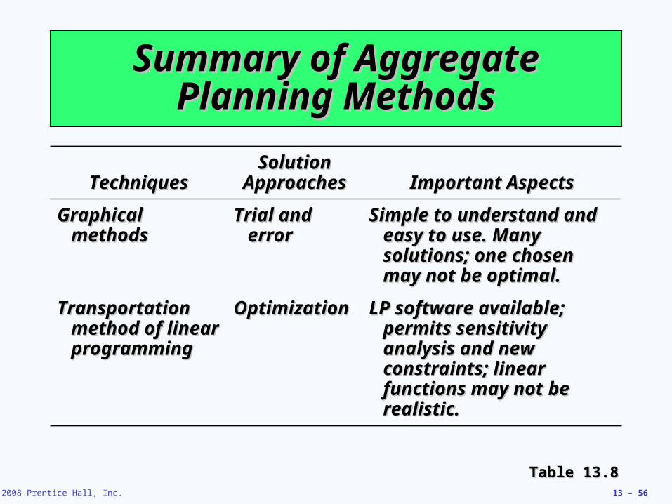
Summary of Aggregate Summary of Aggregate Planning MethodsPlanning Methods
TechniquesTechniquesSolution Solution
ApproachesApproaches Important AspectsImportant Aspects
GraphicalGraphicalmethodsmethods
Trial and Trial and errorerror
Simple to understand and Simple to understand and easy to use. Many easy to use. Many solutions; one chosen solutions; one chosen may not be optimal.may not be optimal.
Transportation Transportation method of linear method of linear programmingprogramming
OptimizationOptimization LP software available; LP software available; permits sensitivity permits sensitivity analysis and new analysis and new constraints; linear constraints; linear functions may not be functions may not be realistic.realistic.
Table 13.8Table 13.8
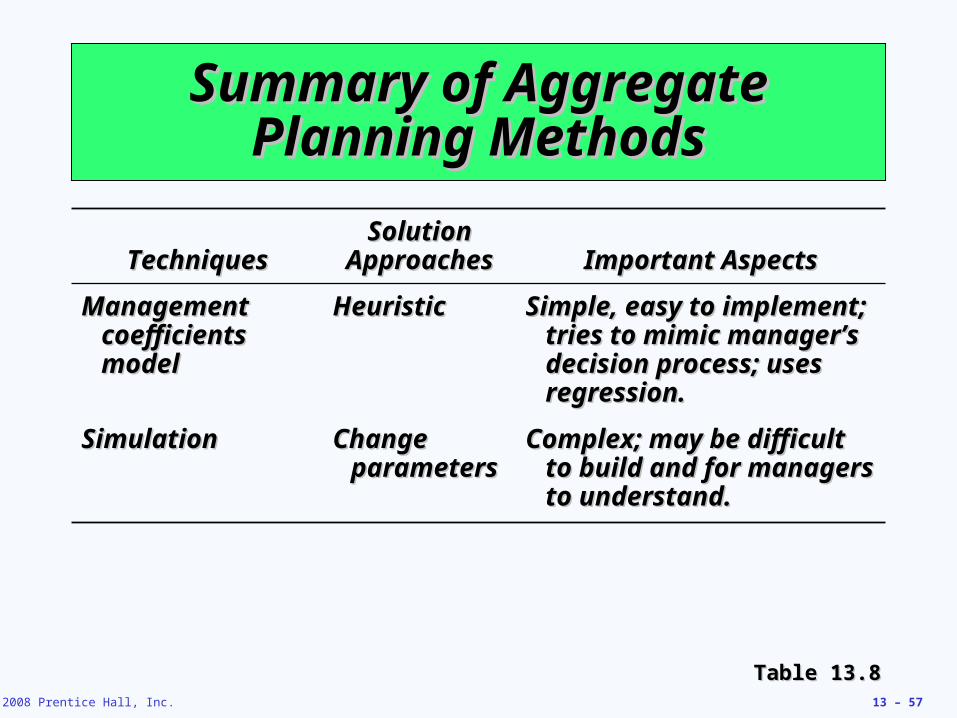
© 2008 Prentice Hall, Inc. 13 – 57
Summary of Aggregate Summary of Aggregate Planning MethodsPlanning Methods
TechniquesTechniquesSolution Solution
ApproachesApproaches Important AspectsImportant Aspects
Management Management coefficients coefficients modelmodel
HeuristicHeuristic Simple, easy to implement; Simple, easy to implement; tries to mimic manager’s tries to mimic manager’s decision process; uses decision process; uses regression.regression.
SimulationSimulation Change Change parametersparameters
Complex; may be difficult Complex; may be difficult to build and for managers to build and for managers to understand.to understand.
Table 13.8Table 13.8
© 2008 Prentice Hall, Inc. 13 – 58
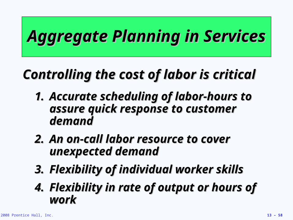
Aggregate Planning in Aggregate Planning in ServicesServices
Controlling the cost of labor is criticalControlling the cost of labor is critical1.1. Accurate scheduling of labor-hours to Accurate scheduling of labor-hours to
assure quick response to customer assure quick response to customer demanddemand
2.2. An on-call labor resource to cover An on-call labor resource to cover unexpected demandunexpected demand
3.3. Flexibility of individual worker skillsFlexibility of individual worker skills4.4. Flexibility in rate of output or hours of Flexibility in rate of output or hours of
workwork
© 2008 Prentice Hall, Inc. 13 – 59
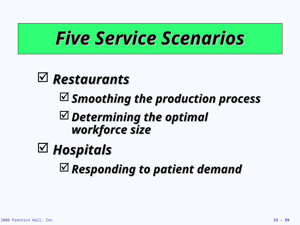
Five Service ScenariosFive Service Scenarios
RestaurantsRestaurants Smoothing the production Smoothing the production
processprocess Determining the optimal Determining the optimal
workforce sizeworkforce size HospitalsHospitals
Responding to patient demandResponding to patient demand

© 2008 Prentice Hall, Inc. 13 – 60
Five Service ScenariosFive Service Scenarios
National Chains of Small Service National Chains of Small Service FirmsFirms Planning done at national level Planning done at national level
and at local leveland at local level Miscellaneous ServicesMiscellaneous Services
Plan human resource Plan human resource requirementsrequirements
Manage demandManage demand

© 2008 Prentice Hall, Inc. 13 – 61
Law Firm ExampleLaw Firm Example
Table 13.9Table 13.9
Labor-Hours RequiredLabor-Hours Required Capacity Constraints Capacity Constraints(2)(2) (3)(3) (4)(4) (5)(5) (6)(6)
(1)(1) ForecastsForecasts MaximumMaximum Number ofNumber ofCategory ofCategory of Best Best LikelyLikely WorstWorst Demand inDemand in QualifiedQualified
Legal BusinessLegal Business (hours)(hours) (hours)(hours) (hours)(hours) PeoplePeople PersonnelPersonnel
Trial workTrial work 1,8001,800 1,5001,500 1,2001,200 3.63.6 44Legal researchLegal research 4,5004,500 4,0004,000 3,5003,500 9.09.0 3232Corporate lawCorporate law 8,0008,000 7,0007,000 6,5006,500 16.016.0 1515Real estate lawReal estate law 1,7001,700 1,5001,500 1,3001,300 3.43.4 66Criminal lawCriminal law 3,5003,500 3,0003,000 2,5002,500 7.07.0 1212Total hoursTotal hours 19,50019,500 17,00017,000 15,00015,000Lawyers neededLawyers needed 3939 3434 3030
© 2008 Prentice Hall, Inc. 13 – 62
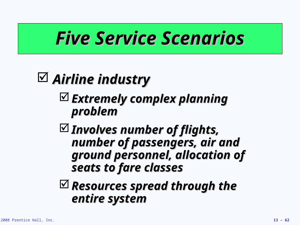
Five Service ScenariosFive Service Scenarios
Airline industryAirline industry Extremely complex planning Extremely complex planning
problemproblem Involves number of flights, Involves number of flights,
number of passengers, air and number of passengers, air and ground personnel, allocation of ground personnel, allocation of seats to fare classesseats to fare classes
Resources spread through the Resources spread through the entire systementire system
© 2008 Prentice Hall, Inc. 13 – 63
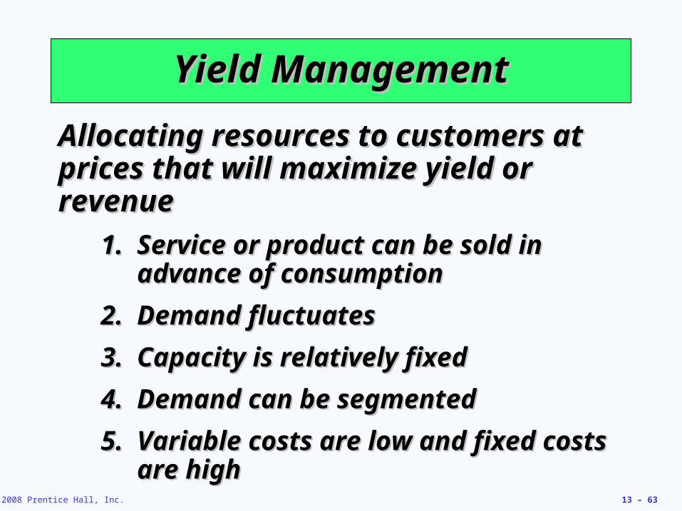
Yield ManagementYield ManagementAllocating resources to customers at Allocating resources to customers at prices that will maximize yield or prices that will maximize yield or revenuerevenue
1.1. Service or product can be sold in Service or product can be sold in advance of consumptionadvance of consumption
2.2. Demand fluctuatesDemand fluctuates3.3. Capacity is relatively fixedCapacity is relatively fixed4.4. Demand can be segmentedDemand can be segmented5.5. Variable costs are low and fixed costs Variable costs are low and fixed costs
are highare high

© 2008 Prentice Hall, Inc. 13 – 64
Demand Demand CurveCurve
Yield Management ExampleYield Management Example
Figure 13.5Figure 13.5
Passed-up contribution
Money left on the table
Potential customers exist who Potential customers exist who are willing to pay more than the are willing to pay more than the $15$15 variable cost of the room variable cost of the room
Some customers who paid Some customers who paid $150$150 were actually willing were actually willing to pay more for the roomto pay more for the roomTotalTotal
$ $ contributioncontribution ==((PricePrice)) x x (50(50roomsrooms))==($150 - $15)($150 - $15)x x (50)(50)==$6,750$6,750
PricePrice
Room salesRoom sales
100100
5050
$150$150Price charged Price charged
for room for room
$15$15Variable costVariable cost
of roomof room
© 2008 Prentice Hall, Inc. 13 – 65
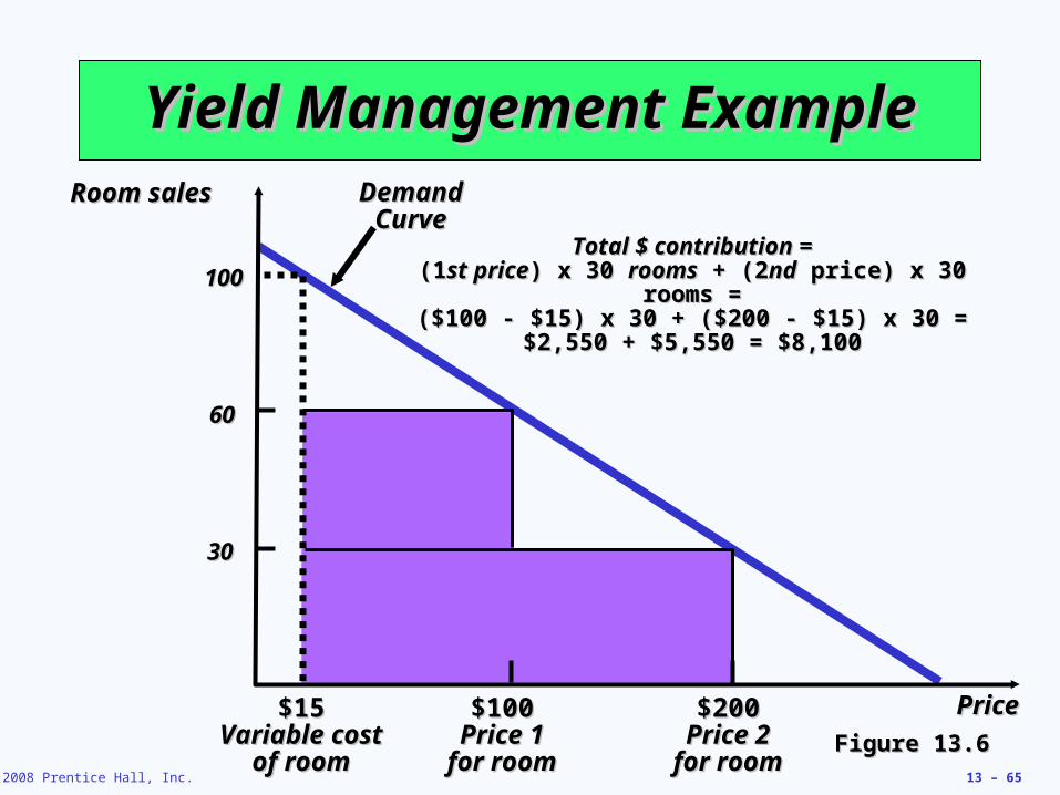
Total $ contribution =Total $ contribution =(1(1st pricest price) x 30 ) x 30 roomsrooms + (2 + (2ndnd price) x 30 rooms = price) x 30 rooms =
($100 - $15) x 30 + ($200 - $15) x 30 =($100 - $15) x 30 + ($200 - $15) x 30 =$2,550 + $5,550 = $8,100$2,550 + $5,550 = $8,100
Demand Demand CurveCurve
Yield Management ExampleYield Management Example
Figure 13.6Figure 13.6PricePrice
Room salesRoom sales
100100
6060
3030
$100$100Price 1Price 1
for roomfor room
$200$200Price 2Price 2
for roomfor room
$15$15Variable costVariable cost
of roomof room

© 2008 Prentice Hall, Inc. 13 – 66
Yield Management MatrixYield Management MatrixD
urat
ion
of u
se
Unp
redi
ctab
le
Pred
icta
ble
PriceTend to be fixed Tend to be variable
Quadrant 1: Quadrant 2:
Movies HotelsStadiums/arenas Airlines
Convention centers Rental carsHotel meeting space Cruise lines
Quadrant 3: Quadrant 4:
Restaurants Continuing careGolf courses hospitals
Internet serviceproviders
Figure 13.7Figure 13.7
© 2008 Prentice Hall, Inc. 13 – 67
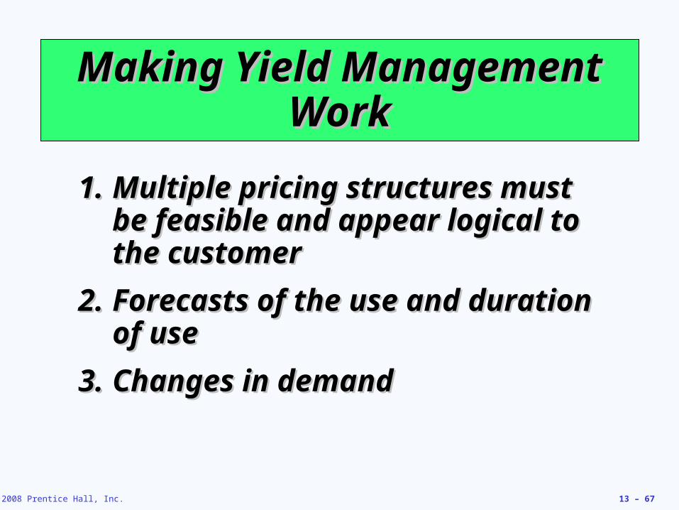
Making Yield Management Making Yield Management WorkWork
1.1. Multiple pricing structures must Multiple pricing structures must be feasible and appear logical to be feasible and appear logical to the customerthe customer
2.2. Forecasts of the use and duration Forecasts of the use and duration of useof use
3.3. Changes in demandChanges in demand
![[PPT]Introduction to Aggregate Planning - University of …rlindek1/POM/Lecture_Slides/AggPlanning... · Web viewPlanning Ch. 3 – Aggregate Planning R. Lindeke UMD Aggregate Planning](https://static.cupdf.com/doc/110x72/5aec7cdc7f8b9ac361908761/pptintroduction-to-aggregate-planning-university-of-rlindek1pomlectureslidesaggplanningweb.jpg)
![[PPT]Introduction to Aggregate Planning - homes.ieu.edu.trhomes.ieu.edu.tr/~agokce/Courses/slides/agregate planning... · Web viewAggregate Planning Introduction to Aggregate Planning](https://static.cupdf.com/doc/110x72/5ade835b7f8b9a595f8e4680/pptintroduction-to-aggregate-planning-homesieuedu-agokcecoursesslidesagregate.jpg)


![[PPT]Production and Operations Management: …sureten/(aggregate planning)5.ppt · Web viewDisaggregating the Aggregate Plan Aggregate Planning Aggregate planning Intermediate-range](https://static.cupdf.com/doc/110x72/5aec86827f8b9ab24d902697/pptproduction-and-operations-management-suretenaggregate-planning5pptweb.jpg)


![[PPT]Introduction to Aggregate Planning - University of …rlindek1/POM/assets/Agg_Chapter03.ppt · Web viewTitle Introduction to Aggregate Planning Author Steven Nahmias Last modified](https://static.cupdf.com/doc/110x72/5ade835b7f8b9a595f8e4679/pptintroduction-to-aggregate-planning-university-of-rlindek1pomassetsagg.jpg)