Advanced R: Visualization andProgramming
Computational Economics PracticeWinter Term 2015/16
Stefan Feuerriegel
Today’s Lecture
Objectives
1 Visualizing data in R graphically as points, lines, contours or areas
2 Understanding the programming concepts of if-conditions and loops
3 Implementing simple functions in R
4 Measuring execution time
2Advanced R

Outline
1 Visualization
2 Control Flow
3 Timing
4 Wrap-Up
3Advanced R

Outline
1 Visualization
2 Control Flow
3 Timing
4 Wrap-Up
4Advanced R: Visualization

Point Plot
I Creating simple point plots (also named scatter plots) via plot(...)I Relies upon vectors denoting the x-axis and y-axis locationsI Various options can be added to change appearance
d <- read.csv("persons.csv", header=TRUE, sep=",",stringsAsFactors=FALSE)
plot(d$height, d$age)
●
●
●●
●
165 170 175 180 185 190
2226
30
d$height
d$ag
e
5Advanced R: Visualization

Adding Title, Labels and Annotations
I Title is added through additional parameter mainI Axis labels are set via xlab and ylabI Annotations next to points with text(...)
plot(d$height, d$age,main="Title", # title for the plotxlab="Height", ylab="Age") # labels for x and y axis
text(d$height, d$age, d$name) # d$name are annotations
●
●
●●
●
165 170 175 180 185 190
2226
30
Title
Height
Age
JuliaRobin
KevinMax
Jerry
6Advanced R: Visualization

Line PlotGenerate line plot using the additional option type="l"
x <- seq(0, 4, 0.01)plot(x, x*x, type="l")
0 1 2 3 4
05
1015
x
x *
x
7Advanced R: Visualization

Exercise: Plotting
x <- seq(-1, +1, 0.01)
−1.0 −0.5 0.0 0.5 1.0
0.0
0.4
0.8
Question
I How would you reproduce the above plot?I plot(x, kink(x), type="l", main="")I plot(x, kink(x), type="l", lab="")I plot(x, abs(x), type="l", ylab="", xlab="")
I Visit http://pingo.upb.de with code 1523
8Advanced R: Visualization

3D Plots
I Consider the function f (x ,y) = x3 +3y− y3−3x
f <- function(x, y) x^3+3*y-y^3-3*x
I Create axis ranges for plotting
x <- seq(-5, 5, 0.1)y <- seq(-5, 5, 0.1)
I Function outer(x,y,f) evaluates f all combinations of x and y
z <- outer(x, y, f)
9Advanced R: Visualization

3D PlotsFunction persp(...) plots the plane through x, y and z in 3D
persp(x, y, z)
x
y
z
10Advanced R: Visualization

3D PlotsTurn on ticks on axes via ticktype="detailed"
persp(x, y, z, ticktype="detailed")
x
−4 −2 0 2 4
y
−4
−2
0
24
z
−200
−100
0
100
200
11Advanced R: Visualization

3D Plots
Parameters theta (left/right) and phi (up/down) control viewing angle
persp(x, y, z, theta=20, phi=0)
x
y
z
persp(x, y, z, theta=20, phi=35)
x
y
z
12Advanced R: Visualization

Contour Plots
I A contour line is a curve along which the function has the same valueI image(...) plots a grid of pixels colored corresponding to z-valueI contour(..., add=TRUE) adds contour lines to an existing plot
image(x, y, z) # Plot colorscontour(x, y, z, add=TRUE) # Add contour lines
−4 −2 0 2 4
−4
−2
02
4
x
y
−150 −100
−50
0 0 0
0
0
0
50
100 150
13Advanced R: Visualization
Contour Plots
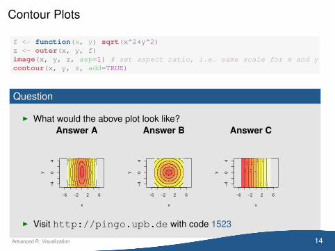
f <- function(x, y) sqrt(x^2+y^2)z <- outer(x, y, f)image(x, y, z, asp=1) # set aspect ratio, i.e. same scale for x and ycontour(x, y, z, add=TRUE)
Question
I What would the above plot look like?Answer A Answer B Answer C
−6 −2 2 6
−4
04
x
y
2
4
6 6
8 8
10 10
12
12
14 14
16
16
−6 −2 2 6
−4
04
x
y
1
2
3
4
5 6
6
6
6
−6 −2 2 6
−4
04
x
y
−0.8
−0.6
−0.4
−0.2
0 0.2
0.4 0.6
0.8
I Visit http://pingo.upb.de with code 1523
14Advanced R: Visualization

Plotting Regression Plane
library(car) # for dataset Highway1
## Warning: no function found corresponding to methods exports from ’SparseM’ for:’coerce’
model <- lm(rate ~ len + slim, data=Highway1)model
#### Call:## lm(formula = rate ~ len + slim, data = Highway1)#### Coefficients:## (Intercept) len slim## 16.61050 -0.09151 -0.20906
x1r <- range(Highway1$len)x1seq <- seq(x1r[1], x1r[2], length=30)x2r <- range(Highway1$slim)x2seq <- seq(x2r[1],x2r[2], length=30)z <- outer(x1seq, x2seq,
function(a,b) predict(model,newdata=data.frame(len=a,slim=b)))
15Advanced R: Visualization

Plotting a Regression Plane
res <- persp(x=x1seq, y=x2seq, z=z,theta=50, phi=-10)
dp <- trans3d(Highway1$len, Highway1$slim,Highway1$rate, pmat=res)
points(dp, pch=20, col="red")
x1seq x2seq
z
●
●●
●●
●
●
●
●
●
●
●●
●●
●●
●
● ● ●●
●
●
●
●
●
●
●
●
●
●●
●
●
●
●
●
●
16Advanced R: Visualization

Outline
1 Visualization
2 Control Flow
3 Timing
4 Wrap-Up
17Advanced R: Control Flow

Managing Code Execution
I Control flow specifies order in which statements are executed
I Previous concepts can only execute R code in a linear fashion
I Control flow constructs can choose which execution path to follow
Functions: Combines sequence of statements into a self-contained task
Conditional expressions: Different computations according to a specificcondition
Loops: Sequence of statements which may be executed more thanonce
18Advanced R: Control Flow

Functions
I Functions avoid repeating the same code more than once
I Leave the current evaluation context to execute pre-defined commands
Main ProgramFunction
19Advanced R: Control Flow

Functions
I Extend set of built-in functions with opportunity for customizationI Functions can consist of the following:
1 Name to refer to (avoid existing function names in R)2 Function body is a sequence of statements3 Arguments define additional parameters passed to the function body4 Return value which can be used after executing the function
I Simple example
f <- function(x,y) {return(2*x + y^2)
}f(-3, 5)
## [1] 19
20Advanced R: Control Flow

Functions
I General syntax
functionname <- function(argument1, argument2, ...) {function_bodyreturn(value)
}
I Return value is the last evaluated expression→ Alternative: set explicitly with return(...)
I Curly brackets can be omitted if the function contains only onestatement (not recommended)
I Be cautious since the order of the arguments matters
I Values in functions are not printed in console→ Remedy is print(...)
21Advanced R: Control Flow

Examples of Functions
square <- function(x) x*x # last value is return valuesquare(10)
## [1] 100
cubic <- function(x) {# Print value to screen from inside the functionprint(c("Value: ", x, " Cubic: ", x*x*x))# no return value
}cubic(10)
## [1] "Value: " "10" " Cubic: " "1000"
22Advanced R: Control Flow

Examples of Functions
hello <- function() { # no argumentsprint("world")
}hello()
## [1] "world"
my.mean <- function(x) {return (sum(x)/length(x))
}my.mean(1:100)
## [1] 50.5
23Advanced R: Control Flow

Scope in Functions
I Variables created inside a function only exists within it→ local
I They are thus inaccessible from outside of the functionI Scope denotes when the name binding of variable is valid
x <- "A"g <- function(x) {x <- "B"return(x)
}x <- "C"
I What are the values?
g(x) # Return value of function xx # Value of x after function execution
I Solution
## [1] "B"## [1] "C"
24Advanced R: Control Flow

Unevaluated Expressions
I Expressions can store symbolic mathematical statements for latermodifications (e. g. symbolic derivatives)
I Let’s define an example via expression(...)
f <- expression(x^3+3*y-y^3-3*x)f
## expression(x^3 + 3 * y - y^3 - 3 * x)
I If evaluation of certain parameters becomes necessary, one can useeval(...)
x <- 2y <- 3eval(f)
## [1] -16
25Advanced R: Control Flow

If-Else Conditions
I Conditional execution requires a condition to be met
Block 1 Block 2
ConditionFalseTrue
26Advanced R: Control Flow

If-Else Conditions
I Keyword if with optional else clause
I General syntax:
if condition
if (condition) {statement1
}
If condition is true,then statement isexecuted
if-else condition
if (condition) {statement1
} else {statement2
}
If condition is true, thenstatement1 is executed,otherwise statement2
27Advanced R: Control Flow

If-Else Conditions
I Example
grade <- 2if (grade <= 4) {print("Passed")
} else {print("Failed")
}
## [1] "Passed"
grade <- 5if (grade <= 4) {print("Passed")
} else {print("Failed")
}
## [1] "Failed"
I Condition must be of length 1 and evaluate as either TRUE or FALSE
if (c(TRUE, FALSE)) { # don't do this!print("something")
}
## Warning in if (c(TRUE, FALSE)) {: Bedingung hat Länge> 1 und nur das erste Element wird benutzt
## [1] "something"
28Advanced R: Control Flow

Else-If Clauses
I Multiple conditions can be checked with else if clauses
I The last else clause applies when no other conditions are fulfilled
I The same behavior can also be achieved with nested if-clauses
else-if clauseif (grade == 1) {print("very good")
} else if (grade == 2) {print("good")
} else {print("not a good grade")
}
Nested if-conditionif (grade == 1) {print("very good")
} else {if (grade == 2) {print("good")
} else {print("not a good grade")
}}
29Advanced R: Control Flow

If-Else Function
I As an alternative, one can also reach the same control flow via thefunction ifelse(...)
ifelse(condition, statement1, statement2)# executes statement1 if condition is true,# otherwise statement2
grade <- 2ifelse(grade <= 4, "Passed", "Failed")
## [1] "Passed"
I ifelse(...) can also work with vectors as if it was applied to eachelement separately
grades <- c(1, 2, 3, 4, 5)ifelse(grades <= 4, "Passed", "Failed")
## [1] "Passed" "Passed" "Passed" "Passed" "Failed"
I This allows for the efficient comparison of vectors
30Advanced R: Control Flow

For Loop
I for loops execute statements for a fixed number of repetitions
Conditional Code
Condition
If condition is false
If condition is true
31Advanced R: Control Flow

For Loop
I General syntax
for (counter in looping_vector){# code to be executed for each element in the sequence
}
I In every iteration of the loop, one value in the looping vector isassigned to the counter variable that can be used in the statementsof the body of the loop.
I Examples
for (i in 4:7) {print(i)
}
## [1] 4## [1] 5## [1] 6## [1] 7
a <- c()for (i in 1:3){a[i] <- sqrt(i)
}a
## [1] 1.000000 1.414214 1.732051
32Advanced R: Control Flow

While Loop
I Loop where the number of iterations is controlled by a conditionI The condition is checked in every iterationI When the condition is met, the loop body in curly brackets is executedI General syntax
while (condition) {# code to be executed
}
I Examples
z <- 1# same behavior as for loopwhile (z <= 4) {
print(z)z <- z + 1
}
## [1] 1## [1] 2## [1] 3## [1] 4
z <- 1# iterates all odd numberswhile (z <= 5) {
z <- z + 2print(z)
}
## [1] 3## [1] 5## [1] 7
33Advanced R: Control Flow

Outline
1 Visualization
2 Control Flow
3 Timing
4 Wrap-Up
34Advanced R: Timing

Measuring Timings via Stopwatch
I Efficiency is a major issue with larger datasets and complex codes
I Timings can help in understanding scalability and bottlenecks
I Use a stopwatch approach measuring the duration between twoproc.time() calls
start.time <- proc.time() # Start the clock
g <- rnorm(100000)h <- rep(NA, 100000)for (i in 1:100000) { # Loop over vector, always add +1h[i] <- g[i] + 1
}
# Stop clock and measure durationduration <- proc.time() - start.time
35Advanced R: Timing

Measuring Timings via Stopwatch
I Results of duration have the following format
## user system elapsed## 0.71 0.02 0.72
I Timings are generally grouped into 3 categoriesI User time measures the understanding of the R instructionsI System time measures the underlying execution timeI Elapsed is the difference since starting the stopwatch (= user +
system)I Alternative approach avoiding loop
start.time <- proc.time() # Start clockg <- rnorm(100000)h <- g + 1proc.time() - start.time # Stop clock
## user system elapsed## 0.08 0.00 0.08
I Rule: vector operations are faster than loops36Advanced R: Timing

Measuring Timings of Function CallsFunction system.time(...) can directly time function calls
slowloop <- function(v){for (i in v) {tmp <- sqrt(i)
}}
system.time(slowloop(1:1000000))
## user system elapsed## 2.06 0.05 2.13
37Advanced R: Timing

Outline
1 Visualization
2 Control Flow
3 Timing
4 Wrap-Up
38Advanced R: Wrap-Up
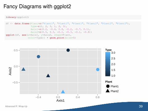
Fancy Diagrams with ggplot2
library(ggplot2)
df <- data.frame(Plant=c("Plant1", "Plant1", "Plant1", "Plant2", "Plant2", "Plant2"),Type=c(1, 2, 3, 1, 2, 3),Axis1=c(0.2, -0.4, 0.8, -0.2, -0.7, 0.1),Axis2=c(0.5, 0.3, -0.1, -0.3, -0.1, -0.8))
ggplot(df, aes(x=Axis1, y=Axis2, shape=Plant,color=Type)) + geom_point(size=5)
●
●
●
−0.5
0.0
0.5
−0.4 0.0 0.4 0.8Axis1
Axi
s2
1.0
1.5
2.0
2.5
3.0Type
Plant
● Plant1
Plant2
39Advanced R: Wrap-Up

Summary: Visualization and Timing
plot() Simple plot function
text() Add text to an existing plot
outer() Apply a function to two arrays
persp() Plot a surface in 3D
image() Plot a colored image
contour() Add contour lines to a plot
trans3d() Add point to an existing 3D plot
points() Add points to a plot
proc.time() Stopwatch for measuring execution time
system.time(expr) Measures execution time of an expression
40Advanced R: Wrap-Up

Summary: Programming
function(){} Self-defined function
expression() Function with arguments not evaluated
eval() Evaluate an expression
if, else Conditional statement
for(){} Loops over a fixed vector
while Loops while a condition is fulfilled
41Advanced R: Wrap-Up

Outlook
Additional Material
I Further exercises as homeworkI Advanced materials beyond our scope
I Advanced R (CRC Press, 2014, by Wickham)http://adv-r.had.co.nz/
Future Exercises
R will be used to implement optimization algorithms
42Advanced R: Wrap-Up