Acoustic seabed classification of marine habitats: studiesin the western coastal-shelf area of Portugal
Rosa Freitas, Susana Silva, Victor Quintino,Ana Maria Rodrigues, Karl Rhynas, and William T. Collins
Freitas, R., Silva, S., Quintino, V., Rodrigues, A. M., Rhynas, K., and Collins, W. T. 2003.Acoustic seabed classification of marine habitats: studies in the western coastal-shelf areaof Portugal. – ICES Journal of Marine Science, 60: 599–608.
Two single-beam, seabed-classification systems, QTC VIEW Series IV and QTC VIEWSeries V, were used to identify and map biosedimentary gradients in a mid-shelf area offWestern Portugal. The survey area has a moderate slope, a depth ranging from 30 to 90malong a 3.5-km axis perpendicular to the shoreline, and is characterized by smooth sedi-mentary and biological gradients. Ground truth for sediment grain size and macrofaunalcommunities was based on grab sampling at 20 sites. The sedimentary and biological datawere analysed using classification and ordination techniques. The acoustic data wereanalysed with QTC IMPACT software and classified into acoustic classes. The affinity groupsobtained in each data set were mapped using a Geographic Information System. All showedgood agreement and identified prevailing gradients along a northwest–southeast direction.Three acoustic classes were identified, corresponding to the predominant sediment types,namely fine sand with low silt and clay content, silty, very fine sand, and mud. A closerelationship with benthic communities was also verified, although less marked becausebenthic communities continuously change along the northwest–southeast gradient. Overall,the acoustic system coupled with ground-truthing data was able to discriminate andcharacterize the various benthic biotopes in the survey area.
� 2003 International Council for the Exploration of the Sea. Published by Elsevier Science Ltd. All rights
reserved.
Keywords: acoustic seabed classification, benthic biotopes, coastal shelf, habitat mapping,Portugal, QTC VIEW.
R. Freitas, S. Silva, V. Quintino, and A. M. Rodrigues: Departamento de Biologia, Centrode Estudos do Ambiente e Mar, Universidade de Aveiro, Aveiro 3810-193, Portugal.K. Rhynas, and W. T. Collins: Quester Tangent Corp., Sidney, B.C., Canada V8L 5Y8.Correspondence to R. Freitas.
Introduction
Recent progress in acoustic technology offers new oppor-
tunities for describing the marine environment. Echosound-
ers and sidescan sonar are commonly used for remote
characterization of the seafloor, including, recently, the
discrimination of benthic biotopes (Kenny et al., 2003).
Tools such as QTC VIEW and RoxAnn process the acous-
tic signals from single-beam echosounders and output data
to Geographic Information Systems (GIS) to map differ-
ences in seafloor characteristics (Greenstreet et al., 1997;
Hamilton et al., 1999; Kloser et al., 2001; Anderson et al.,
2002).
The QTC VIEW Series IV and Series V seabed-
classification systems used in this study are powerful tools
for the discrimination of marine benthic habitats. Several
studies have shown their response to bottom features such
as sediment grain size and compactness, seabed roughness,
bedrock, benthic organisms, and bottom slope (Collins
et al., 1996; Hamilton et al., 1999; Preston et al., 1999;
Preston, 2001; Anderson et al., 2002; Ellingsen et al., 2002;
von Szalay and McConnaughey, 2002). Most of these
studies covered areas with a variety of contrasting bottom
features with sharp discontinuities. Recently, their effi-
ciency was assessed in an area of relative seascape mono-
tony, viz. in a sand and gravel, nearshore shelf area, with
very low silt content (Freitas et al., 2003). In this present
study, both acoustic systems were used in a mid-shelf area
with a smooth biological gradient and sediment grain size
ranging from clean, fine sand to mud with silt and clay
content above 75%, with a view to comparing the results of
the QTC VIEW Series IV and Series V systems.
YJMSC1393_proof � 3 June 2003 � 12:48 am
ICES Journal of Marine Science, 60: 599–608. 2003doi:10.1016/S1054–3139(03)00061-4
1054–3139/03/000599þ10 $30.00 � 2003 International Council for the Exploration of the Sea. Published by Elsevier Science Ltd. All rights reserved.
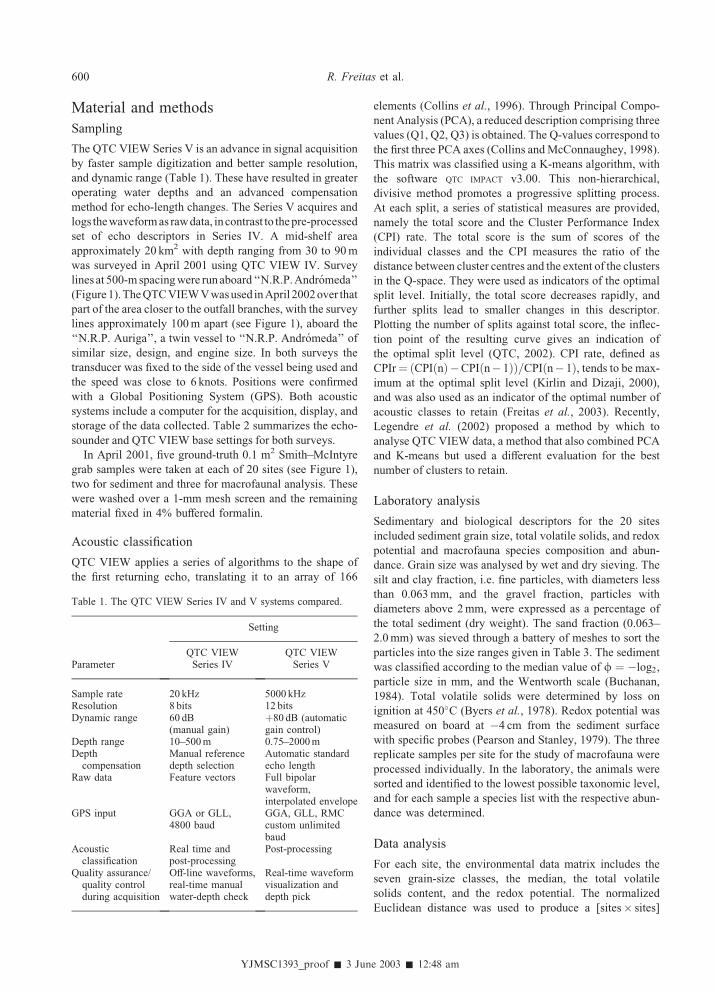
Material and methods
Sampling
The QTC VIEW Series V is an advance in signal acquisition
by faster sample digitization and better sample resolution,
and dynamic range (Table 1). These have resulted in greater
operating water depths and an advanced compensation
method for echo-length changes. The Series V acquires and
logs thewaveformas rawdata, incontrast to thepre-processed
set of echo descriptors in Series IV. A mid-shelf area
approximately 20 km2 with depth ranging from 30 to 90m
was surveyed in April 2001 using QTC VIEW IV. Survey
lines at 500-mspacingwere run aboard ‘‘N.R.P.Andromeda’’
(Figure1).TheQTCVIEWVwasused inApril 2002over that
part of the area closer to the outfall branches, with the survey
lines approximately 100m apart (see Figure 1), aboard the
‘‘N.R.P. Auriga’’, a twin vessel to ‘‘N.R.P. Andromeda’’ of
similar size, design, and engine size. In both surveys the
transducer was fixed to the side of the vessel being used and
the speed was close to 6 knots. Positions were confirmed
with a Global Positioning System (GPS). Both acoustic
systems include a computer for the acquisition, display, and
storage of the data collected. Table 2 summarizes the echo-
sounder and QTC VIEW base settings for both surveys.
In April 2001, five ground-truth 0.1 m2 Smith–McIntyre
grab samples were taken at each of 20 sites (see Figure 1),
two for sediment and three for macrofaunal analysis. These
were washed over a 1-mm mesh screen and the remaining
material fixed in 4% buffered formalin.
Acoustic classification
QTC VIEW applies a series of algorithms to the shape of
the first returning echo, translating it to an array of 166
elements (Collins et al., 1996). Through Principal Compo-
nent Analysis (PCA), a reduced description comprising three
values (Q1, Q2, Q3) is obtained. The Q-values correspond to
the first three PCA axes (Collins andMcConnaughey, 1998).
This matrix was classified using a K-means algorithm, with
the software QTC IMPACT v3.00. This non-hierarchical,
divisive method promotes a progressive splitting process.
At each split, a series of statistical measures are provided,
namely the total score and the Cluster Performance Index
(CPI) rate. The total score is the sum of scores of the
individual classes and the CPI measures the ratio of the
distance between cluster centres and the extent of the clusters
in the Q-space. They were used as indicators of the optimal
split level. Initially, the total score decreases rapidly, and
further splits lead to smaller changes in this descriptor.
Plotting the number of splits against total score, the inflec-
tion point of the resulting curve gives an indication of
the optimal split level (QTC, 2002). CPI rate, defined as
CPIr¼ ðCPIðnÞ�CPIðn� 1ÞÞ=CPIðn� 1Þ, tends to be max-
imum at the optimal split level (Kirlin and Dizaji, 2000),
and was also used as an indicator of the optimal number of
acoustic classes to retain (Freitas et al., 2003). Recently,
Legendre et al. (2002) proposed a method by which to
analyse QTC VIEW data, a method that also combined PCA
and K-means but used a different evaluation for the best
number of clusters to retain.
Laboratory analysis
Sedimentary and biological descriptors for the 20 sites
included sediment grain size, total volatile solids, and redox
potential and macrofauna species composition and abun-
dance. Grain size was analysed by wet and dry sieving. The
silt and clay fraction, i.e. fine particles, with diameters less
than 0.063mm, and the gravel fraction, particles with
diameters above 2mm, were expressed as a percentage of
the total sediment (dry weight). The sand fraction (0.063–
2.0mm) was sieved through a battery of meshes to sort the
particles into the size ranges given in Table 3. The sediment
was classified according to the median value of / ¼ �log2,
particle size in mm, and the Wentworth scale (Buchanan,
1984). Total volatile solids were determined by loss on
ignition at 450�C (Byers et al., 1978). Redox potential was
measured on board at �4 cm from the sediment surface
with specific probes (Pearson and Stanley, 1979). The three
replicate samples per site for the study of macrofauna were
processed individually. In the laboratory, the animals were
sorted and identified to the lowest possible taxonomic level,
and for each sample a species list with the respective abun-
dance was determined.
Data analysis
For each site, the environmental data matrix includes the
seven grain-size classes, the median, the total volatile
solids content, and the redox potential. The normalized
Euclidean distance was used to produce a [sites� sites]
YJMSC1393_proof � 3 June 2003 � 12:48 am
Table 1. The QTC VIEW Series IV and V systems compared.
Setting
ParameterQTC VIEWSeries IV
QTC VIEWSeries V
Sample rate 20 kHz 5000 kHzResolution 8 bits 12 bitsDynamic range 60 dB
(manual gain)þ80 dB (automaticgain control)
Depth range 10–500m 0.75–2000mDepthcompensation
Manual referencedepth selection
Automatic standardecho length
Raw data Feature vectors Full bipolarwaveform,interpolated envelope
GPS input GGA or GLL,4800 baud
GGA, GLL, RMCcustom unlimitedbaud
Acousticclassification
Real time andpost-processing
Post-processing
Quality assurance/quality controlduring acquisition
Off-line waveforms,real-time manualwater-depth check
Real-time waveformvisualization anddepth pick
600 R. Freitas et al.
distance matrix submitted to classification analysis using
the average-clustering algorithm and to ordination analysis
using non-metric, multidimensional scaling (MDS). Both
used the software PRIMER v5 (Clarke and Gorley, 2001).
The biological data were represented by a matrix of
20 sites per 119 variables, corresponding to the species
abundances. After square-root transformation, the [sites�sites] Bray–Curtis similarity matrix was classified with the
average-clustering algorithm. Ordination was done by cor-
respondence analysis using the software MVSP v3.12d
(Kovach, 1999).
The classification output files representing the acoustic
diversity were analysed in ARC VIEW 8.1. For this, the final
output files from both surveys were opened separately in
a spreadsheet and the echo description, latitude and longi-
tude, class name, class confidence, and class probability
were selected from the appropriate fields. The data were
sorted first by confidence level, and those under 98% were
deleted. The confidence value is the probability that
a record belongs to the class to which it has been assigned,
rather than to any other class. Based on Bayes’ theorem,
this value is a measure of the covariance-weighted dis-
tances between the position of the record in Q-space and
the positions of all cluster centres (QTC, 2002). The
resulting file was further sorted by the probability and
values under 1% were ignored. The probability value of
YJMSC1393_proof � 3 June 2003 � 12:48 am
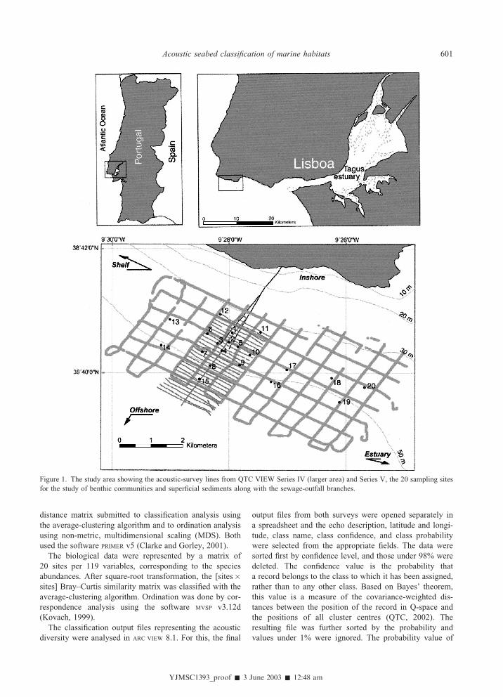
Figure 1. The study area showing the acoustic-survey lines from QTC VIEW Series IV (larger area) and Series V, the 20 sampling sites
for the study of benthic communities and superficial sediments along with the sewage-outfall branches.
601Acoustic seabed classification of marine habitats
a record is based on the position of that record in the Q-
space and the characteristics of the class to which it has
been assigned. This is a measure of the closeness of the
record to the cluster centre, weighted by the covariance of
the cluster in the direction of the record. Probability and
confidence calculations are based on Bayes’ theorem and the
assumption that the underlying distribution in Q-space is
Gaussian (QTC, 2002). The acoustic, sediment, and macro-
fauna plots were overlapped to facilitate comparison.
Results
Sedimentary gradients
The classification and ordination analysis of the environ-
mental data is displayed in Figure 2, and a summary
YJMSC1393_proof � 3 June 2003 � 12:49 am
Table 2. Survey base-settings for both echosounders and acousticsystems. (AGC, automatic gain control.)
Setting
Parameter
QTC VIEWSeries IV
(NRP Andromeda)
QTC VIEWSeries V
(NRP Auriga)
Echosounder
Beam width 44� 19�
Transmit power 150W 100WPulse duration 625ls 300lsPing rate 5 per s 5 per sFrequency 50 kHz 50 kHz
QTCVIEW
Base gain 5 dB AGC
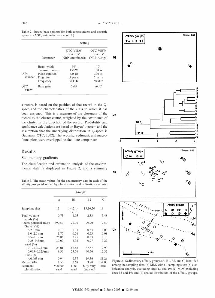
Table 3. The mean values for the sedimentary data in each of theaffinity groups identified by classification and ordination analysis.
Groups
A B1 B2 C
Sampling sites 13 1–12,14,17,18
15,16,20 19
Total volatilesolids (%)
0.73 1.05 2.33 5.48
Redox potential (mV) 390.50 129.70 79.20 �7.50Gravel (%)
>2.0mm 0.13 0.31 0.63 0.031.0–2.0mm 3.77 0.76 0.53 0.080.5–1.0mm 25.86 2.25 0.53 0.180.25–0.5mm 37.00 4.92 0.77 0.27
Sand (%)0.125–0.25mm 23.01 65.68 37.57 2.900.063–0.125mm 9.30 23.76 40.70 15.33
Fines (%)<0.063mm 0.94 2.37 19.36 81.26
Median (U) 1.55 2.68 3.20 >4.00Sedimentclassification
Mediumsand
Finesand
Silty veryfine sand
Mud
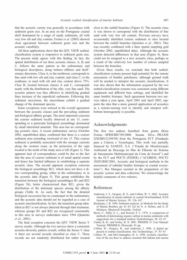
Figure 2. Sedimentary affinity groups (A, B1, B2, and C) identified
among the sampling sites. (a) MDS with all sampling sites; (b) clas-
sification analysis, excluding sites 13 and 19; (c) MDS excluding
sites 13 and 19; and (d) spatial distribution of the affinity groups.
602 R. Freitas et al.
characterization of each group is given in Table 3. When
including all the sampling sites in the analysis, three groups
were separated in the ordination diagram (Figure 2a): group
A (site 13), group C (site 19), and group B (the remaining
sites). Sites 13 and 19 over-dominate the ordination pattern
because of their particular grain size. The coarser sediment
was observed at site 13, the only site classified as medium
sand, and site 19 had a silt/clay fraction much higher than
elsewhere (Table 3). Excluding these two sites from the
analysis, group B is further subdivided into subgroups B1
and B2, as shown in the classification and ordination
diagrams (Figure 2b, c). The spatial distribution of the
major affinity groups (A, B1, B2, C) is shown in Figure 2d.
Along the axis A ! B1 ! B2 ! C, the superficial sedi-
ments show gradual increases in the median value, the silt
and clay content, and the total volatile solids, while the
redox potential decreases (Table 3). Most of the superficial
sediments in the study area correspond to fine sand with
low silt and clay content (subgroup B1). With increasing
depth (inshore–offshore axis, cf. Figure 1) and towards the
estuary (shelf–estuary axis, cf. Figure 1), the superficial
sediment becomes silty, very fine sand (subgroup B2), and
finally mud (group C) (cf. Table 3).
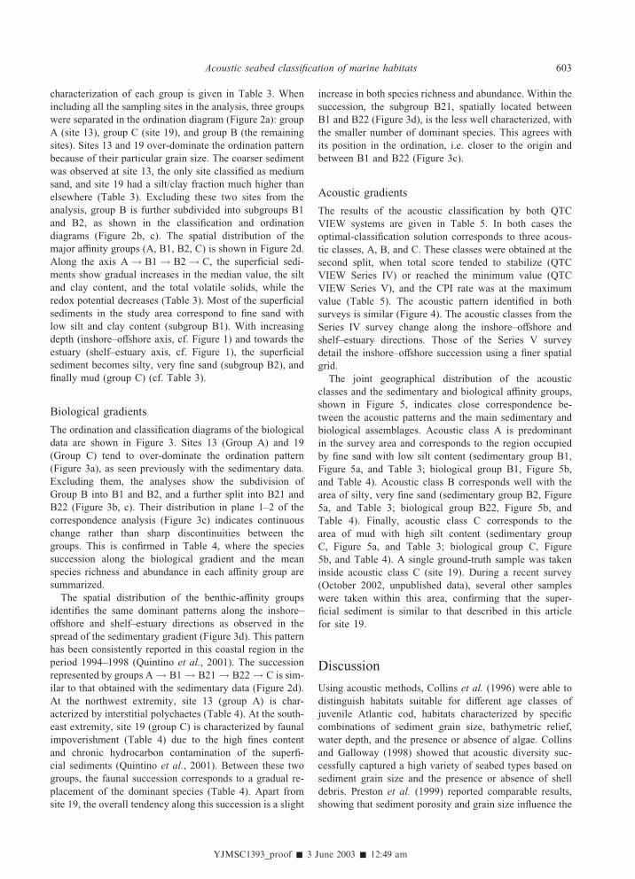
Biological gradients
The ordination and classification diagrams of the biological
data are shown in Figure 3. Sites 13 (Group A) and 19
(Group C) tend to over-dominate the ordination pattern
(Figure 3a), as seen previously with the sedimentary data.
Excluding them, the analyses show the subdivision of
Group B into B1 and B2, and a further split into B21 and
B22 (Figure 3b, c). Their distribution in plane 1–2 of the
correspondence analysis (Figure 3c) indicates continuous
change rather than sharp discontinuities between the
groups. This is confirmed in Table 4, where the species
succession along the biological gradient and the mean
species richness and abundance in each affinity group are
summarized.
The spatial distribution of the benthic-affinity groups
identifies the same dominant patterns along the inshore–
offshore and shelf–estuary directions as observed in the
spread of the sedimentary gradient (Figure 3d). This pattern
has been consistently reported in this coastal region in the
period 1994–1998 (Quintino et al., 2001). The succession
represented by groups A ! B1 ! B21 ! B22 ! C is sim-
ilar to that obtained with the sedimentary data (Figure 2d).
At the northwest extremity, site 13 (group A) is char-
acterized by interstitial polychaetes (Table 4). At the south-
east extremity, site 19 (group C) is characterized by faunal
impoverishment (Table 4) due to the high fines content
and chronic hydrocarbon contamination of the superfi-
cial sediments (Quintino et al., 2001). Between these two
groups, the faunal succession corresponds to a gradual re-
placement of the dominant species (Table 4). Apart from
site 19, the overall tendency along this succession is a slight
increase in both species richness and abundance. Within the
succession, the subgroup B21, spatially located between
B1 and B22 (Figure 3d), is the less well characterized, with
the smaller number of dominant species. This agrees with
its position in the ordination, i.e. closer to the origin and
between B1 and B22 (Figure 3c).
Acoustic gradients
The results of the acoustic classification by both QTC
VIEW systems are given in Table 5. In both cases the
optimal-classification solution corresponds to three acous-
tic classes, A, B, and C. These classes were obtained at the
second split, when total score tended to stabilize (QTC
VIEW Series IV) or reached the minimum value (QTC
VIEW Series V), and the CPI rate was at the maximum
value (Table 5). The acoustic pattern identified in both
surveys is similar (Figure 4). The acoustic classes from the
Series IV survey change along the inshore–offshore and
shelf–estuary directions. Those of the Series V survey
detail the inshore–offshore succession using a finer spatial
grid.
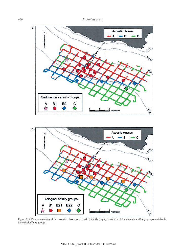
The joint geographical distribution of the acoustic
classes and the sedimentary and biological affinity groups,
shown in Figure 5, indicates close correspondence be-
tween the acoustic patterns and the main sedimentary and
biological assemblages. Acoustic class A is predominant
in the survey area and corresponds to the region occupied
by fine sand with low silt content (sedimentary group B1,
Figure 5a, and Table 3; biological group B1, Figure 5b,
and Table 4). Acoustic class B corresponds well with the
area of silty, very fine sand (sedimentary group B2, Figure
5a, and Table 3; biological group B22, Figure 5b, and
Table 4). Finally, acoustic class C corresponds to the
area of mud with high silt content (sedimentary group
C, Figure 5a, and Table 3; biological group C, Figure
5b, and Table 4). A single ground-truth sample was taken
inside acoustic class C (site 19). During a recent survey
(October 2002, unpublished data), several other samples
were taken within this area, confirming that the super-
ficial sediment is similar to that described in this article
for site 19.
Discussion
Using acoustic methods, Collins et al. (1996) were able to
distinguish habitats suitable for different age classes of
juvenile Atlantic cod, habitats characterized by specific
combinations of sediment grain size, bathymetric relief,
water depth, and the presence or absence of algae. Collins
and Galloway (1998) showed that acoustic diversity suc-
cessfully captured a high variety of seabed types based on
sediment grain size and the presence or absence of shell
debris. Preston et al. (1999) reported comparable results,
showing that sediment porosity and grain size influence the
YJMSC1393_proof � 3 June 2003 � 12:49 am
603Acoustic seabed classification of marine habitats
acoustic response. Hamilton et al. (1999) found that the
bottom classes suggested by the acoustic system had con-
sistent grain size and texture properties and followed grain-
size trends. The work of Ellingsen et al. (2002) showed
YJMSC1393_proof � 3 June 2003 � 12:49 am
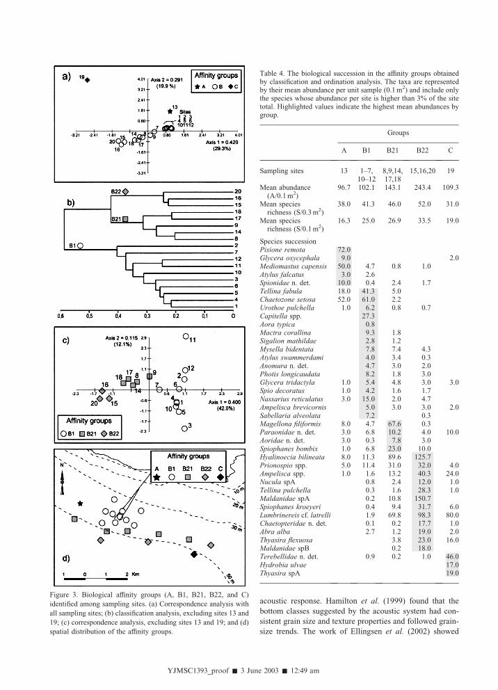
Figure 3. Biological affinity groups (A, B1, B21, B22, and C)
identified among sampling sites. (a) Correspondence analysis with
all sampling sites; (b) classification analysis, excluding sites 13 and
19; (c) correspondence analysis, excluding sites 13 and 19; and (d)
spatial distribution of the affinity groups.
Table 4. The biological succession in the affinity groups obtainedby classification and ordination analysis. The taxa are representedby their mean abundance per unit sample (0.1m2) and include onlythe species whose abundance per site is higher than 3% of the sitetotal. Highlighted values indicate the highest mean abundances bygroup.
Groups
A B1 B21 B22 C
Sampling sites 13 1–7,10–12
8,9,14,17,18
15,16,20 19
Mean abundance(A/0.1m2)
96.7 102.1 143.1 243.4 109.3
Mean speciesrichness (S/0.3m2)
38.0 41.3 46.0 52.0 31.0
Mean speciesrichness (S/0.1m2)
16.3 25.0 26.9 33.5 19.0
Species successionPisione remota 72.0Glycera oxycephala 9.0 2.0Mediomastus capensis 50.0 4.7 0.8 1.0Atylus falcatus 3.0 2.6Spionidae n. det. 10.0 0.4 2.4 1.7Tellina fabula 18.0 41.3 5.0Chaetozone setosa 52.0 61.0 2.2Urothoe pulchella 1.0 6.2 0.8 0.7Capitella spp. 27.3Aora typica 0.8Mactra corallina 9.3 1.8Sigalion mathildae 2.8 1.2Mysella bidentata 7.8 7.4 4.3Atylus swammerdami 4.0 3.4 0.3Anomura n. det. 4.7 3.0 2.0Photis longicaudata 8.2 1.8 3.0Glycera tridactyla 1.0 5.4 4.8 3.0 3.0Spio decoratus 1.0 4.2 1.6 1.7Nassarius reticulatus 3.0 15.0 2.0 4.7Ampelisca brevicornis 5.0 3.0 3.0 2.0Sabellaria alveolata 7.2 0.3Magellona filiformis 8.0 4.7 67.6 0.3Paraonidae n. det. 3.0 6.8 10.2 4.0 10.0Aoridae n. det. 3.0 0.3 7.8 3.0Spiophanes bombix 1.0 6.8 23.0 10.0Hyalinoecia bilineata 8.0 11.3 89.6 125.7Prionospio spp. 5.0 11.4 31.0 32.0 4.0Ampelisca spp. 1.0 1.6 13.2 40.3 24.0Nucula spA 0.8 2.4 12.0 1.0Tellina pulchella 0.3 1.6 28.3 1.0Maldanidae spA 0.2 10.8 150.7Spiophanes kroeyeri 0.4 9.4 31.7 6.0Lumbrinereis cf. latrelli 1.9 69.8 98.3 80.0Chaetopteridae n. det. 0.1 0.2 17.7 1.0Abra alba 2.7 1.2 19.0 2.0Thyasira flexuosa 3.8 23.0 16.0Maldanidae spB 0.2 18.0Terebellidae n. det. 0.9 0.2 1.0 46.0Hydrobia ulvae 17.0Thyasira spA 19.0
YJMSC1393_proof � 3 June 2003 � 12:49 am
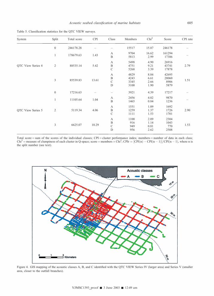
Table 5. Classification statistics for the QTC VIEW surveys.
System Split Total score CPI Class Members Chi2 Score CPI rate
QTC View Series 4
0 246178.28 – – 15517 15.87 246178 –
1 178679.63 1.43A 9704 16.62 161294
–B 5813 2.99 17386
2 88535.14 5.42A 5498 4.90 26916
2.79B 4751 9.21 43741C 5268 3.39 17878
3 85539.83 13.61
A 4829 8.84 42695
1.51B 4243 6.61 28060C 3345 2.66 8906D 3100 1.90 5879
QTC View Series 5
0 17216.63 – – 3921 4.39 17217 –
1 11105.64 1.04A 2456 4.02 9870
–B 1465 0.84 1236
2 5119.34 4.06A 1551 1.09 1692
2.90B 1259 1.37 1726C 1111 1.53 1701
3 6625.07 10.29
A 1100 2.09 2304
1.53B 916 1.14 1043C 949 0.81 770D 956 2.62 2508
Total score¼ sum of the scores of the individual classes; CPI¼ cluster performance index; members¼ number of data in each class;Chi2¼measure of clumpiness of each cluster in Q-space; score¼members�Chi2; CPIr ¼ ½CPIðnÞ � CPIðn� 1Þ�=CPIðn� 1Þ, where n isthe split number (see text).
Figure 4. GIS mapping of the acoustic classes A, B, and C identified with the QTC VIEW Series IV (larger area) and Series V (smaller
area, closer to the outfall branches).
605Acoustic seabed classification of marine habitats
YJMSC1393_proof � 3 June 2003 � 12:49 am
Figure 5. GIS representation of the acoustic classes A, B, and C, jointly displayed with the (a) sedimentary affinity groups and (b) the
biological affinity groups.
606 R. Freitas et al.
that the acoustic variety was generally in accordance with
sediment grain size. In an area on the Portuguese coastal
shelf dominated by a range of sandy sediments, all with
very low silt and clay content, Freitas et al. (2003) showed
close agreement between sediment grain size and the
acoustic variability.
All these applications show that the QTC VIEW seabed-
classification system is responsive to sediment grain size.
The present study agrees with this finding. In fact, the
spatial distribution of our three acoustic classes, A, B, and
C, follows the same pattern as the sedimentary and
biological descriptors, along inshore–offshore and shelf–
estuary directions. Class A, to the northwest, corresponds to
fine sand with low silt and clay content, and class C, to the
southeast, to mud with silt and clay content above 75%.
Class B, located between classes A and C, corresponds
neatly with the distribution of the silty, very fine sand. The
acoustic pattern was thus effective in identifying gradual
fines increase of the superficial sediments. Following this
sediment succession, the macrofauna exhibit a gradual
change of the dominant species.
Some exceptions were noticed in the overall agreement
between the acoustic classes and the prevailing sediment
and biological affinity groups. The most important concerns
the coarser sediment locally observed at site 13, corre-
sponding to a particular biological assemblage dominated
by small interstitial annelids. This area has no correspond-
ing acoustic class. A recent sedimentary survey (October
2002, unpublished data), confirmed that there is a coarser
sediment area extending westward of site 13. This coarser
sediment is probably associated with the stronger currents
along the western coast, as the protection of the cape
located to the north of the study area is left (Figure 1). This
apparent lack of correspondence could be due to the fact
that the area of coarser sediment is of small spatial extent
and hence has limited influence in establishing a separate
acoustic class. The second apparent exception concerns
the biological assemblage B21, which does not have a di-
rect corresponding group, either in the sedimentary or in
the acoustic data (Figure 5). This group establishes the
transition between the biological assemblages B1 and B22
(Figure 5b), better characterized than B21, given the
distribution of the dominant species among the affinity
groups (Table 4). As such, the fact that the detailed
biological succession has no counterpart in the sedimentary
and the acoustic data should not be regarded as a case of
acoustic misclassification. In fact, the transition group iden-
tified as B21 is not always detected through data treatment,
whereas groups B1 and B22 are recognized consistently
in this area in surveys undertaken since 1994 (Quintino
et al., 2001).
The final exception concerns the QTC VIEW Series V
survey results. Although the two surveys show a consistent
acoustic-diversity pattern overall, within the Series V class
A there are several records classified as class C. These
records are not randomly distributed but rather located
close to the outfall branches (Figure 4). The acoustic class
A was shown to correspond with the distribution of fine
sand with very low silt content. Previous surveys have
occasionally identified coarser sediment in sites located
between the outfall branches (Quintino et al., 2001). This
was recently confirmed with a finer spatial sampling grid
(October 2002, unpublished data). Although the acoustic
system detected differences in that area (Figure 4), these
could not be assigned to a new acoustic class, perhaps as
a result of the relatively low number of echoes sampled
between the branches.
Given these results, we conclude that both seabed-
classification systems present high potential for the remote
assessment of benthic patchiness, although ground truth
will be needed to interpret the acoustic classifications. It
was also shown that the information acquired by the two
seabed-classification systems was consistent using different
equipment and different base settings, and identified the
same benthic biotopes. Such agreement between two sur-
veys taken a year apart, April 2001 and April 2002, sup-
ports the idea that a more general application of acoustics
as a remote-sensing tool to identify and interpret soft-
bottom heterogeneity is possible.
Acknowledgements
The first two authors benefited from grants (Rosa
Freitas—SFRH/BD/769/2000; Susana Silva—PRAXIS
XXI/BD/21298/99) from the Portuguese FCT (Fundacao
para a Ciencia e Tecnologia). This work was partially
financed by SANEST, S.A. (‘‘Estudo de Monitorizacao
Ambiental da Descarga no Mar do Efluente do Sistema
de Saneamento Multimunicipal da Costa do Estoril’’) and
by the FCT and POCTI (FEDER) (‘‘ACOBIOS, POCTI/
38203/BSE/2001, Acoustic and biological methods in the
assessment of subtidal benthic biotopes in coastal ecosys-
tems’’). Rui Marques assisted in the preparation of the
acoustic system and data collection. We acknowledge the
helpful comments of two referees.
References
Anderson, J. T., Gregory, R. S., and Collins, W. T. 2002. Acousticclassification of marine habitats in coastal Newfoundland. ICESJournal of Marine Science, 59: 156–167.
Buchanan, J. B. 1984. Sediment analysis. In Methods for the Studyof Marine Benthos, pp. 41–65. Ed. by N. A. Holme, and A. D.McIntyre. Blackwell Scientific, Oxford.
Byers, C., Mills, E. L., and Stewart, P. L. 1978. A comparison ofmethods of determining organic carbon in marine sediments withsuggestions for a standard method. Hydrobiologia, 58: 43–47.
Clarke, K. R., and Gorley, R. N. 2001. PRIMER v5: User Manual/Tutorial. PRIMER-E, Plymouth. 91 pp.
Collins, W., Gregory, R., and Anderson, J. 1996. A digital ap-proach to seabed classification. Sea Technolology, 37: 83–87.
Collins, W., and McConnaughey, R. A. 1998. Acoustic classifica-tion of the sea floor to address essential fish habitat and marine
YJMSC1393_proof � 3 June 2003 � 12:50 am
607Acoustic seabed classification of marine habitats
protected area requirements. Proceedings of the CanadianHydrographic Conference, Victoria, B.C., Canada. pp. 369–377.
Ellingsen, K. E., Gray, J. S., and Bjørnbom, E. 2002. Acousticclassification of seabed habitat using the QTC VIEWTM system.ICES Journal of Marine Science, 59: 825–835.
Freitas, R., Rodrigues, A. M., and Quintino, V. 2003. Benthicbiotopes remote sensing using acoustics. Journal of Experimen-tal Marine Biology and Ecology 285–286: 339–353.
Greenstreet, S. P. R., Tuck, I. D., Grewar, G. N., Armstrong, E.,Reid, D. G., andWright, P. J. 1997. An assessment of the acousticsurvey technique, RoxAnn, as a means of mapping seabedhabitat. ICES Journal of Marine Science, 54: 939–959.
Hamilton, L. J., Mulhearn, P. J., and Poeckert, R. 1999. Com-parison of RoxAnn and QTC-View acoustic bottom classifica-tion system performance for the Cairns area, Great Barrier Reef,Australia. Continental Shelf Research, 19: 1577–1597.
Kenny, A. J., Cato, I., Desprez, M., Fader, G., Schuttenhelm, R. T.E., and Side, J. 2003. An overview of seabed mapping tech-nologies in the context of marine habitat classification. ICESJournal of Marine Science, 60: 411–418.
Kirlin, R. L., and Dizaji, R. M. 2000. Cluster order using clusteringperformance index rate, CPIR. Proceedings NORSIG 2000,Kolmarden, Sweden. pp. 85–88.
Kloser, R. J., Bax, N. J., Ryan, T., Williams, A., and Barker, B. A.2001. Remote sensing of seabed types in the Australian SouthEast Fishery; development and application of normal incidentacoustic techniques and associated ‘‘ground truthing’’. Marineand Freshwater Research, 52: 475–489.
Kovach, W. L. 1999. MVSP: A Multivariate Statistical Packagefor Windows, Ver. 3.1. User’s Manual. Kovach ComputingServices, Pentraeth, Wales, UK. 133 pp.
Legendre, P., Ellingsen, K. E., Bjornborn, E., and Casgrain, P. 2002.Acoustic seabed classification: improved statistical method.Canadian Journal ofFisheries andAquatic Science, 59: 1085–1089.
Pearson, T. H., and Stanley, S. O. 1979. Comparative measurementof the redox potential of marine sediments as a rapid means ofassessing the effect of organic pollution. Marine Biology, 53:371–379.
Preston, J. 2001. Shallow-water bottom classification. High speedecho-sampling captures detail for precise sediment. HydroInternational, 5: 30–33.
Preston, J. M., Collins, W. C., Mosher, D. C., Poeckert, R. H., andKuwahara, R. H. 1999. The strengh of correlations betweengeotechnical variables and acoustic classifications. Proceedingsof Oceans ’99, 3: 1123–1127.
QTC 2002. QTC IMPACT. Acoustic Seabed Classification. UserGuide. Version 3.20, July 2002. Quester Tangent Corporation,Marine Technology Centre, Sidney, B.C., Canada. 110 pp.
Quintino, V., Rodrigues, A. M., Re, A., Pestana, M. P., Silva, S., andCastro, H. 2001. Sediment alterations in response to marineoutfall operation off Lisbon, Portugal: a sediment quality triadstudy. Journal of Coastal Research, 34: 535–549 (Special issue).
von Szalay, P. G., and McConnaughey, R. A. 2002. The effect ofslope and vessel speed on the performance of a single beamacoustic seabed classification system. Fisheries Research, 54:181–194.
YJMSC1393_proof � 3 June 2003 � 12:50 am
608 R. Freitas et al.