University of South FloridaScholar Commons
Graduate Theses and Dissertations Graduate School
January 2013
Accelerated Fuzzy ClusteringJonathon Karl ParkerUniversity of South Florida, [email protected]
Follow this and additional works at: http://scholarcommons.usf.edu/etd
Part of the Computer Sciences Commons
This Dissertation is brought to you for free and open access by the Graduate School at Scholar Commons. It has been accepted for inclusion inGraduate Theses and Dissertations by an authorized administrator of Scholar Commons. For more information, please [email protected].
Scholar Commons CitationParker, Jonathon Karl, "Accelerated Fuzzy Clustering" (2013). Graduate Theses and Dissertations.http://scholarcommons.usf.edu/etd/4929
Accelerated Fuzzy Clustering
by
Jonathon Karl Parker
A dissertation submitted in partial fulfillmentof the requirements for the degree of
Doctor of PhilosophyDepartment of Computer Science and Engineering
College of EngineeringUniversity of South Florida
Major Professor: Lawrence Hall, Ph.D.Dmitry Goldgof, Ph.D.Sudeep Sarkar, Ph.D.
Bo Zeng, Ph.D.Joni Downs, Ph.D.
Date of Approval:November 4, 2013
Keywords: fuzzy c-means, scalable, statistical sampling, stopping criterion, representative object
Copyright c© 2013, Jonathon Karl Parker

Dedication
for my son, James

Acknowledgments
“you don’t forget, because you always remember”- Lawrence “Yogi” Berra [1]
This dissertation would not have been possible without the support and encouragement from
my wife, Ann.
I acknowledge and thank my major professor, Dr. Lawrence Hall, for his patience and mentor-
ship over the years. I would also like to acknowledge my committee members, Dr. Dmitry Goldgof,
Dr. Sudeep Sarkar, Dr. Bo Zeng, and Dr. Joni Downs, for their attention to detail and advice.
Faculty members of the University of South Florida deserve special mention. I deeply appreciate
the knowledge and patience of Dr. Rahul Tripathi, the insight and optimism of Dr. Abraham
Kandel, the wisdom and kindness of Dr. Rafael Perez, the hard-earned praise of Dr. Nagarajan
Ranganathan, and the fruitful collaboration with Dr. Joni Downs. I would also like to thank Dr.
Carlos Otero for our engaging, but brief time working together.
I also wish to thank Dr. Kurt Kramer for his infinite patience and plankton data, Dr. Tim
Havens for his assistance, and Dr. James Bezdek for his encouragement and praise.
Table of Contents
List of Tables v
List of Figures vii
Abstract ix
Chapter 1 Introduction 11.1 Cluster Analysis 11.2 Handling Big Data 31.3 Contributions 51.4 Organization 6
Chapter 2 Background 72.1 Basic Clustering Algorithms 7
2.1.1 Single Linkage (SL) 72.1.1.1 Runtime Complexity 11
2.1.2 Hard c-means (HCM) 112.1.2.1 Runtime Complexity 14
2.1.3 Density Based Spatial Clustering of Applications with Noise(DBSCAN) 152.1.3.1 Runtime Complexity 17
2.2 Algorithms Based on Fuzzy Sets 182.2.1 Fuzzy Sets and Logic 182.2.2 Fuzzy c-means (FCM) 19
2.2.2.1 Runtime Complexity 202.2.3 Fuzzy c-medoids (FCMdd) 20
2.2.3.1 Runtime Complexity 232.2.4 Fuzzy Neighborhood DBSCAN (FN-DBSCAN) 24
2.3 Accelerated Clustering Algorithms 272.3.1 Significant Work Related to Acceleration 27
2.3.1.1 Relational Clustering 292.3.2 Single Pass Fuzzy c-means (SPFCM) 30
2.3.2.1 Runtime Complexity 312.3.3 Online Fuzzy c-means (OFCM) 312.3.4 Extensible Fast Fuzzy c-means (eFFCM) 32
2.3.4.1 Runtime Complexity 332.3.5 Random Sampling Plus Extension Fuzzy c-means (rseFCM) 342.3.6 Density Based Distributed Clustering (DBDC) 34
i
2.3.7 Scalable DBDC (SDBDC) 352.4 Evaluation Metrics 36
2.4.1 Relative Speedup (SU) 372.4.2 Difference in Quality of Objective Function 372.4.3 Cluster Change Percentage 382.4.4 Difference in Fidelity of Partitions 402.4.5 Adjusted Rand Index (ARI) 402.4.6 Accuracy 422.4.7 Some Statistics 42
2.4.7.1 Welch’s t-test 422.4.7.2 Z-test 43
Chapter 3 Datasets 443.1 About the Datasets 443.2 MRI Datasets 443.3 Plankton Datasets 453.4 UCI Datasets 46
3.4.1 Breast Cancer (Wisconsin) 473.4.2 Heart-Statlog 473.4.3 Iris 473.4.4 Landsat 473.4.5 Letters 473.4.6 Pendigits 483.4.7 Vote 48
3.5 Artificial 483.5.1 D3C6 Series 493.5.2 D4C5 49
Chapter 4 A Simple Experiment 504.1 Introduction 504.2 Experimental Procedures 504.3 Results 524.4 Discussion 52
4.4.1 rseFCM’s Speedup 544.4.2 eFFCM’s Speedup 554.4.3 SPFCM’s Speedup 574.4.4 OFCM’s Speedup 58
4.5 Conclusions 624.5.1 Assessing Quality 624.5.2 Ranking the Algorithms 634.5.3 Observations 64
Chapter 5 Accelerating FCM 675.1 Estimating the Random Sample Size 675.2 Algorithms Based on Thompson’s Method 705.3 The GOFCM Algorithm 71
ii
5.4 The MSERFCM Algorithm 78
5.4.1 Runtime Complexity 79
5.5 The MODSPFCM Algorithm 79
5.6 Experiments 80
5.6.1 Experimental Procedures 81
5.6.2 Results 84
5.7 GOFCM vs. Related Methods 95
5.8 Artificial Datasets and OFCM 100
5.8.1 MSERFCM 103
5.8.2 Plankton Dataset Challenges 105
Chapter 6 Accelerating FCMdd 107
6.1 Distributed FCMdd 107
6.1.1 Linking Methods 108
6.1.2 Discussion 109
6.1.3 Runtime Complexity 110
6.2 Experiments 111
6.2.1 Experimental Procedures 112
6.2.2 Parameters 113
6.2.3 Results 113
6.3 Discussion 116
6.3.1 The Artificial Datasets 116
6.3.2 Speedup 118
6.3.3 Quality Issues 120
6.3.3.1 Estimated Sample Size 123
Chapter 7 Accelerating FN-DBSCAN 127
7.1 Accelerating a Density-Based Algorithm 127
7.2 Experiments 129
7.3 Results 130
7.4 Discussion 130
7.4.1 Reducing MinCard 132
7.4.2 Cluster Splitting and Aggregation 133
7.4.3 Selecting the Number of Subsets 134
7.4.4 Conclusions 135
Chapter 8 Summary and Conclusions 137
8.1 Summary 137
8.2 Conclusions 139
References 142
Appendices 150
Appendix A Algorithm Implementations 151
A.1 Introduction 151
A.2 Fuzzy c-means Codebase 151
iii

A.2.1 Termination Criterion 152A.2.2 eFFCM 154A.2.3 Kolen’s Optimization 155
A.3 Fuzzy c-medoids Codebase 155A.4 Fuzzy Neighborhood DBSCAN Codebase 156
Appendix B Expanded Results 157
iv
List of Tables
Table 3.1 Datasets 45
Table 3.2 Configuration Data for D4C5 49
Table 4.1 Experiment Parameter Settings 51
Table 4.2 Speedup Comparison for MRI016, fPDA = 0.05 52
Table 4.3 Average Performance vs. FCM on MRI Datasets 53
Table 4.4 Average Performance vs. FCM on Pendigits Dataset 53
Table 4.5 Average Performance vs. FCM on Landsat Dataset 54
Table 4.6 rseFCM Speedup vs. FCM with Overhead 55
Table 4.7 Averaged Results for eFFCM and rseFCM 56
Table 4.8 SPFCM Performance 58
Table 4.9 OFCM Performance 59
Table 4.10 Average Performance of OFCM vs. SPFCM 60
Table 5.1 Experiment Parameter Settings 83
Table 5.2 MRI Speedup 84
Table 5.3 MRI Speedup (Ignoring Randomization and I/O) 85
Table 5.4 D6C5 Speedup 86
Table 5.5 D10C7 Speedup 86
Table 5.6 PLK01 Speedup 89
Table 5.7 MODSPFCM MRI Speedup 92
Table 5.8 MODSPFCM D6C5 Speedup 92
Table 5.9 MODSPFCM D10C7 Speedup 92
v
Table 5.10 MODSPFCM PLK01 Speedup 93
Table 5.11 Comparison with Havens’ Results 101
Table 5.12 Speedup over Range of σ (MRI016) 102
Table 6.1 Linking Methods 109
Table 6.2 Speedups for MRI016R 114
Table 6.3 DFCMdd Speedup by Linking Methods 114
Table 6.4 DFCMdd Speedup Omitting D3C6-1 115
Table 6.5 DFCMdd Artificial Dataset Results 116
Table 6.6 DFCMdd Real-World Dataset Results 117
Table 6.7 FCMdd Clustering Results for Artificial Datasets 117
Table 6.8 Speedups for Plankton 120
Table 6.9 Runtimes for D3C6 Datasets 120
Table 6.10 Sample Size Estimates from Thompson’s Formula 123
Table 6.11 Quality Results for MRI017R 124
Table 6.12 Quality Results for PLK02 126
Table 7.1 AFN-DBSCAN Parameters 130
Table 7.2 AFN-DBSCAN Results 131
Table 7.3 AFN-DBSCAN Pendigits Results 131
Table B.1 Complete DFCMdd Artificial Dataset Results 157
Table B.2 Complete DFCMdd Real-World Dataset Results 158
Table B.3 Complete MRI016 Results 159
Table B.4 Complete MRI017 Results 160
Table B.5 Complete MRI018 Results 161
vi
List of Figures
Figure 1.1 A Simple Clustering Scenario 2
Figure 1.2 A Fuzzy Clustering Scenario 3
Figure 2.1 Clustering with Single Linkage 10
Figure 2.2 Single Linkage Chaining 11
Figure 2.3 Clustering with Hard c-means 14
Figure 2.4 Data Objects xp and xq Have Same Density in DBSCAN, but HaveDifferent Densities in FN-DBSCAN 25
Figure 2.5 Linear Neighborhood Function Used in FN-DBSCAN 26
Figure 5.1 Cluster Center Position Change 75
Figure 5.2 Log of Change in V for GOFCM and Dataset MRI017 77
Figure 5.3 DQRm% (MRI) 85
Figure 5.4 Cluster Center Change % (MRI) 86
Figure 5.5 DQRm% (D6C5) 87
Figure 5.6 DQRm% (D10C7) 87
Figure 5.7 Cluster Center Change % (D6C5) 88
Figure 5.8 Cluster Center Change % (D10C7) 88
Figure 5.9 DQRm% (PLK01) 89
Figure 5.10 Cluster Center Change % (PLK01) 90
Figure 5.11 DQRm% (MRI) 93
Figure 5.12 DQRm% (C6D5) 94
Figure 5.13 DQRm% (C10D7) 95
vii
Figure 5.14 DQRm% (PLK01) 96
Figure 5.15 Cluster Center Change % (MRI) 97
Figure 5.16 Cluster Center Change % (D6C5) 98
Figure 5.17 Cluster Center Change % (D10C7) 99
Figure 5.18 Cluster Center Change % (PLK01) 100
Figure 5.19 DQRm% over Range of σ (MRI016) 102
Figure 5.20 Cluster Center Change % over Range of σ (MRI016) 103
viii
Abstract
Clustering algorithms are a primary tool in data analysis, facilitating the discovery of groups
and structure in unlabeled data. They are used in a wide variety of industries and applications.
Despite their ubiquity, clustering algorithms have a flaw: they take an unacceptable amount of
time to run as the number of data objects increases. The need to compensate for this flaw has led
to the development of a large number of techniques intended to accelerate their performance. This
need grows greater every day, as collections of unlabeled data grow larger and larger.
How does one increase the speed of a clustering algorithm as the number of data objects increases
and at the same time preserve the quality of the results? This question was studied using the Fuzzy
c-means clustering algorithm as a baseline. Its performance was compared to the performance of
four of its accelerated variants. Four key design principles of accelerated clustering algorithms
were identified. Further study and exploration of these principles led to four new and unique
contributions to the field of accelerated fuzzy clustering. The first was the identification of a
statistical technique that can estimate the minimum amount of data needed to ensure a multinomial,
proportional sample. This technique was adapted to work with accelerated clustering algorithms.
The second was the development of a stopping criterion for incremental algorithms that minimizes
the amount of data required, while maximizing quality. The third and fourth techniques were new
ways of combining representative data objects. Five new accelerated algorithms were created to
demonstrate the value of these contributions.
One additional discovery made during the research was that the key design principles most often
improve performance when applied in tandem. This discovery was applied during the creation of
the new accelerated algorithms. Experiments show that the new algorithms improve speedup
with minimal quality loss, are demonstrably better than related methods and occasionally are an
improvement in both speedup and quality over the base algorithm.
ix
Chapter 1: Introduction
“You’ve got to be careful if you don’t know where you’re going, ’cause you might not get there.”
- Lawrence “Yogi” Berra [2]
1.1 Cluster Analysis
Cluster analysis is an exploratory technique used to discover groups and structure in a set of
data objects [3] [4]. A data object can represent any object of interest, but there is one caveat: It
must be possible to measure the similarity (or dissimilarity) of one object to another. Each data
object will have one or more features associated with it. For example, a dataset of athletes might
record: age, height, and weight as some of its features.
A clustering algorithm accepts as input a dataset and produces as output a set of cluster
assignments for all data objects in the dataset. A set of assignments to clusters is also referred to
as a partition of the data. But what is a cluster? Intuition tells you that a cluster is a group of data
objects, which are more similar to each other than to other objects in the dataset [3] [4]. There are
many different types of clustering algorithms. One taxonomy used classifies clustering algorithms
as hierarchical or partitional; though each class of algorithm has subclassifications [3]. Under the
partitional classification, there is a subclass that seeks to minimize an objective functional value
[5]. Another subclassification consists of those that are density-based.
Three of the most common clustering algorithms of the hierarchical, objective function mini-
mization, and density-based types are discussed in detail in Section 2.1.
Cluster analysis is used to explore data in a wide variety of disciplines [5]. A non exhaustive
list includes grouping web-based news articles [6], image processing [7], literature-based discovery
1
[8], marketing [9], medical research [10] [11], military intelligence [12], oil exploration [13], and
psychology [14].
A human being has little difficulty finding groups of data objects, especially when a small
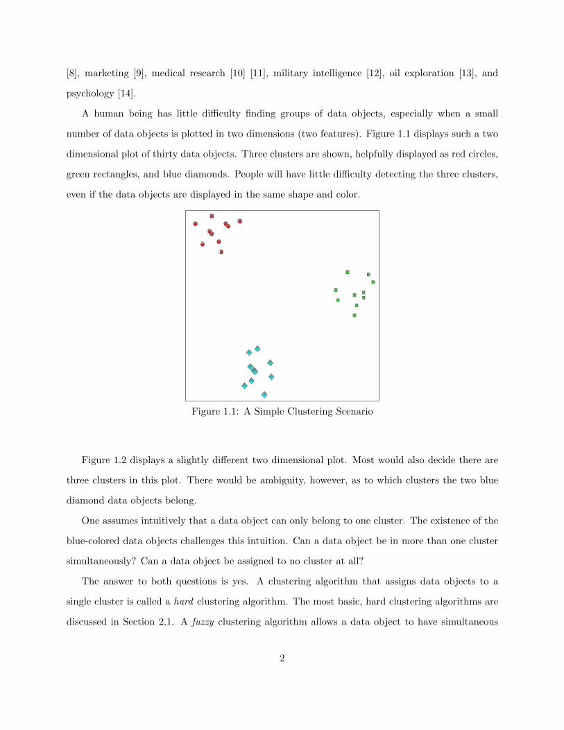
number of data objects is plotted in two dimensions (two features). Figure 1.1 displays such a two
dimensional plot of thirty data objects. Three clusters are shown, helpfully displayed as red circles,
green rectangles, and blue diamonds. People will have little difficulty detecting the three clusters,
even if the data objects are displayed in the same shape and color.
Figure 1.1: A Simple Clustering Scenario
Figure 1.2 displays a slightly different two dimensional plot. Most would also decide there are
three clusters in this plot. There would be ambiguity, however, as to which clusters the two blue
diamond data objects belong.
One assumes intuitively that a data object can only belong to one cluster. The existence of the
blue-colored data objects challenges this intuition. Can a data object be in more than one cluster
simultaneously? Can a data object be assigned to no cluster at all?
The answer to both questions is yes. A clustering algorithm that assigns data objects to a
single cluster is called a hard clustering algorithm. The most basic, hard clustering algorithms are
discussed in Section 2.1. A fuzzy clustering algorithm allows a data object to have simultaneous
2
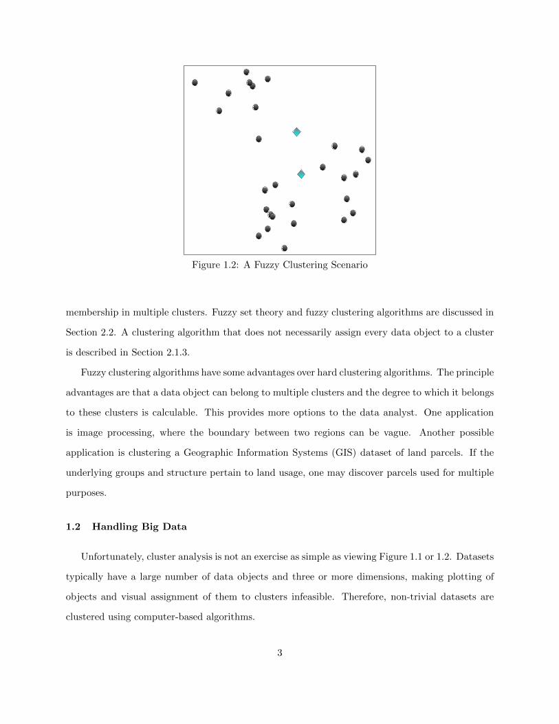
Figure 1.2: A Fuzzy Clustering Scenario
membership in multiple clusters. Fuzzy set theory and fuzzy clustering algorithms are discussed in
Section 2.2. A clustering algorithm that does not necessarily assign every data object to a cluster
is described in Section 2.1.3.
Fuzzy clustering algorithms have some advantages over hard clustering algorithms. The principle
advantages are that a data object can belong to multiple clusters and the degree to which it belongs
to these clusters is calculable. This provides more options to the data analyst. One application
is image processing, where the boundary between two regions can be vague. Another possible
application is clustering a Geographic Information Systems (GIS) dataset of land parcels. If the
underlying groups and structure pertain to land usage, one may discover parcels used for multiple
purposes.
1.2 Handling Big Data
Unfortunately, cluster analysis is not an exercise as simple as viewing Figure 1.1 or 1.2. Datasets
typically have a large number of data objects and three or more dimensions, making plotting of
objects and visual assignment of them to clusters infeasible. Therefore, non-trivial datasets are
clustered using computer-based algorithms.
3
Electronic datasets have been growing in size for decades. Huber discussed in 1994 a clas-
sification system for dataset sizes, which ended with the term “monster” to describe a dataset
having 1012 data objects [15]. Such a system proved unsuitable for Havens, who extends Huber’s
classification with the Very Large (VL) dataset, which has > 1012 data objects [16].
The larger volumes of data available today are typically called “Big Data” [17]. The definitions
for Big Data are generally subjective.
Madden offers such a subjective definition for Big Data. He describes Big Data as data “too big,
too fast, or too hard for existing tools to process” [18]. So the conception of Big Data is relative to
one’s power to deal with it. Jacobs defines Big Data in this context by its effects, namely as “data
whose size forces us to look beyond the tried and true methods that are prevalent at the time” [19].
Ratner states that Big Data is in the mind of the data analyst; how much data is needed for it
to be “Big” is subjective. He then goes on to describe necessary qualities of data to be considered
“Big.” One quality comes from the field of classical statistics, where the sample size is so large that
the “asymptotic properties of the method kick in for valid results” [20].
In summary, a Big Data dataset is cumbersome because of its size, but valuable because of the
information it potentially contains.
Clustering algorithms are only one of many analytic tools that can be applied to Big Data.
The runtime for a typical clustering algorithm will scale linearly to quadratically, with respect to
the number of data objects. The larger the dataset, the longer the algorithm will take to produce
a partition. Processing the entire dataset with typical clustering algorithms can be infeasible for
real-world applications, taking more time than a required decision about the data allows.
Techniques are therefore needed to accelerate the clustering algorithms. A related challenge is
to preserve the quality of the clustering algorithm’s results while accelerating its operation simul-
taneously. The quality should be equivalent to clustering all the data with a classical algorithm.
These areas are the subject of this dissertation.
I used large datasets for experimentation, but not truly “Big Data.” An implied task is to report
the differences in runtime and quality of the accelerated clustering algorithms when compared to
basic algorithms. If the datasets were so large as to be Big Data, the runtime of the basic algorithms
4
on the full datasets would preclude receiving results in a timely fashion. Thus, I infer from the
runtime complexity of the algorithms and the results of smaller scale experiments, the expected
performance on Big Data.
1.3 Contributions
I investigated the key algorithm design principles that accelerate fuzzy clustering algorithms
while preserving quality. Quality is defined as closely approximating well known fuzzy clustering
algorithms. My investigation identified four main ideas to apply to the development of accelerated
fuzzy clustering algorithms on Big Data:
1. Use of a statistically significant sample of the dataset reduces runtime while preserving quality.
2. An algorithm designed to cluster the data incrementally can produce a high-quality result
when stopped before all data has been processed. This is especially true when the data is
presented in random order.
3. The use of representative objects, either weighted or un-weighted, can overcome difficulties
of scale, if properly utilized.
4. For a particular class of clustering algorithms, providing a “starting point” close to the optimal
solution reduces runtime and can improve quality.
None of these ideas are original. All are sound, previously-used tools for the construction
of accelerated clustering algorithms. The contributions made in this dissertation are unique, fully
developed, implemented strategies to employ these ideas to accelerate fuzzy clustering. The specific
contributions of this dissertation are as follows:
• Identification of a statistical method never before used with accelerated fuzzy clustering al-
gorithms. This method estimates the minimum sample size required to represent each cluster
proportionally. I modified the statistical formula to make it compatible with clustering algo-
rithms.
5
• Creation of an early stopping criterion for incremental or “single pass” algorithms. This
criterion determines the point at which processing additional data will have little added
benefit. This allows the clustering algorithm to terminate early, providing a greater speedup
with little loss in quality.
• Different methods of combining representative objects were explored using fuzzy clustering al-
gorithms which produce partitions by minimizing an objective function. I discovered that the
best method used information from the intermediate results to improve quality and speedup.
• I developed a new method to combine representative objects in the context of density-based
fuzzy clustering algorithms.
• I created five original algorithms that apply these contributions and the four main ideas listed
above.
1.4 Organization
In Chapter 2, I provide detailed background on relevant clustering algorithms, accelerated
variants, and metrics used to assess performance. In Chapter 3, I describe the data used for
experiments.
In Chapter 4, a series of exploratory experiments are documented. Observations made from the
experimental results were condensed into the four main ideas identified above.
In Chapters 5, 6, and 7 these ideas are developed into the specific contributions made to the
field of Computer Science. To demonstrate the value of these contributions, five original algorithms
we created implemented these contributions. Experimentation and discussion are included.
Chapter 8 summarizes my work and concludes the dissertation.
6

Chapter 2: Background
“It’s deja vu all over again.” - Lawrence “Yogi” Berra [2]
2.1 Basic Clustering Algorithms
Many clustering algorithms have been developed over the last five decades [5]. Only a relatively
small number of algorithms out of the number available could be chosen to be the focus of my
dissertation. One can categorize the choices by considering different types of clustering algorithms.
A taxonomy of clustering algorithms was described by Jain [3]. One distinction made in his tax-
onomy is whether the clustering algorithm is hierarchical or partitional. A hierarchical algorithm
produces a nested grouping of partitions; at each level of the hierarchy there is a different number
of clusters. A partitional algorithm produces a single partition with a fixed number of clusters.1
One can distinguish partitional algorithms as to whether the basis for partition is minimizing
an objective function or density-based [3] [5]. In a density-based algorithm, clusters are defined as
regions of high density, separated by regions of low density [24, 5].
Three of the most basic clustering algorithms of these types are described below. Each basic
algorithm selected is the original or best-known representative of its type: hierarchical (Single
Linkage), objective function minimizing (Hard c-means), and density-based (DBSCAN).
2.1.1 Single Linkage (SL)
Of the three basic algorithms, Single Linkage is the oldest. The first work that suggests Single
Linkage, initially published in French and Polish in 1951, was rediscovered in 1957 and published
in English [25].
1Some of the material in this chapter has been previously published by me [21] [22] [23], and is re-used underterms of the copyright c© 2010, 2012 and 2013 IEEE.
7

Single Linkage, also referred to as “Single Link” or “Nearest Neighbor,” is a hierarchical, ag-
glomerative clustering algorithm. It employs a dissimilarity coefficient, ρ(xi, xj), that defines the
degree to which two data objects in dataset X are dissimilar [26]. For numeric data, ρ(xi, xj) is
often a distance metric, such as the Euclidean distance.
At the beginning of the algorithm, each data object in the dataset (xi ∈ X) is considered to
be its own cluster. The algorithm merges into a single cluster the two clusters (which initially are
data objects) that are least dissimilar. Single Linkage repeats the merging of the least dissimilar
clusters until all n data objects in X have been assigned to a single cluster.
A formal description, adapted from [27], is presented as Algorithm 1. For efficiency, implemen-
tations of the algorithm usually store the dissimilarities in a dissimilarity matrix.
The algorithm returns a list of merges, M . The decision to merge two clusters is based on the
dissimilarity coefficient. Thus, given a dataset, a dissimilarity coefficient, and rules for tie-breaking,
Single Linkage is deterministic in that it will always return the same list of merges [27].
Single Linkage begins with n clusters. With each merge, the number of clusters is reduced by
1. If the cluster assignments prior to each merge are listed, a numeric hierarchy of height n− 1 is
created. A dendrogram is the most common way to display a hierarchy.
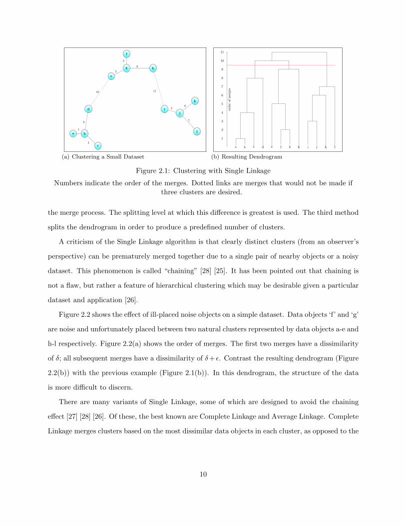
This process is shown in Figure 2.1. Figure 2.1(a) shows a simple dataset consisting of 12 data
objects. Merges are indicated by line segments connecting two data objects. Each line segment
is annotated with a number to show the order of the merges. Note that data objects a and b are
connected with a line segment annotated with a ‘1’. This is the first merge. Likewise, the ‘2’
between objects f and g indicates the second merge. All n− 1 merges are shown in Figure 2.1(a).
Figure 2.1(b) shows the dendrogram that displays the hierarchical structure created by Single
Linkage. The y axis shows the order of the merges connecting data objects. The number assigned
to the merge is also called a splitting level [25].
A human would typically consider the dataset shown in Figure 2.1(a) as having three clusters.
If Single Linkage were halted after splitting level 9, the merges labeled ‘10’ and ‘11’ would not
be made and three clusters would remain. The red line in Figure 2.1(b) shows the effect on the
dendrogram.
8

Algorithm 1: Single Linkage
1: Input: X, ρ(xi, xj)2: for i = 1 to n do3: L[i] = i (each initial cluster is labeled with the index of its data object)4: for j = 1 to i do5: D(xi, xj) = D(xj , xi) = ρ(xi, xj)6: end for7: end for8: for k = 1 to n− 1 do9: (a, b) = argmin(a,b):D(a,b)6=−1D(a, b)
10: M.append(a, b)11: D(a, b) = D(b, a) = −112: for j = 1 to n do13: if L[j] = b then14: L[b] = a (cluster b is now part of cluster a)15: end if16: D(a, xj) = D(b, xj) = min(D(a, xj), D(b, xj))17: end for18: end for19: return M
where:X is a dataset consisting of n data objects.ρ(xi, xj) is the dissimilarity coefficient.xi is the ith data object in X.D is the dissimilarity matrix and D(xi, xj) is the dissimilarity between xi and xj .D(a, b) = −1 indicates objects a and b are in the same cluster.L is an array holding the current set of cluster labels.M is an ordered list holding the pairs of merges.
If the dataset is small, examining a dendrogram visually can reveal the number of clusters.
When the dataset is larger, some method is needed in order to split the hierarchy represented
by the dendrogram. Three of the many methods for splitting the dendrogram are described by
Manning [27].
The first method splits the dendrogram at a user-defined value of dissimilarity. Note that the
dissimilarity between objects increases monotonically as they are merged by Algorithm 1. Thus, if
a particular value of dissimilarity were exceeded, all subsequent merges would be of this value or
greater. The second method calculates the difference between the successive dissimilarities during
9
a b
c
d
e
f
g h
ij
k
l1
2
3
4
5
6
78
9
10 11
(a) Clustering a Small Dataset
a b c d e f g h i j k l
order
ofm
erge
s
1
2
3
4
5
6
7
8
9
10
11
(b) Resulting Dendrogram
Figure 2.1: Clustering with Single Linkage
Numbers indicate the order of the merges. Dotted links are merges that would not be made ifthree clusters are desired.
the merge process. The splitting level at which this difference is greatest is used. The third method
splits the dendrogram in order to produce a predefined number of clusters.
A criticism of the Single Linkage algorithm is that clearly distinct clusters (from an observer’s
perspective) can be prematurely merged together due to a single pair of nearby objects or a noisy
dataset. This phenomenon is called “chaining” [28] [25]. It has been pointed out that chaining is
not a flaw, but rather a feature of hierarchical clustering which may be desirable given a particular
dataset and application [26].
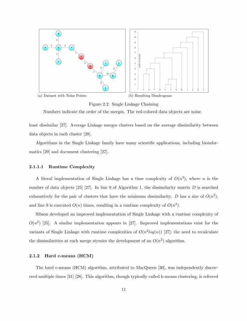
Figure 2.2 shows the effect of ill-placed noise objects on a simple dataset. Data objects ‘f’ and ‘g’
are noise and unfortunately placed between two natural clusters represented by data objects a-e and
h-l respectively. Figure 2.2(a) shows the order of merges. The first two merges have a dissimilarity
of δ; all subsequent merges have a dissimilarity of δ+ ε. Contrast the resulting dendrogram (Figure
2.2(b)) with the previous example (Figure 2.1(b)). In this dendrogram, the structure of the data
is more difficult to discern.
There are many variants of Single Linkage, some of which are designed to avoid the chaining
effect [27] [28] [26]. Of these, the best known are Complete Linkage and Average Linkage. Complete
Linkage merges clusters based on the most dissimilar data objects in each cluster, as opposed to the
10
a b
c
d
e
f
g
h
i
j
k
l
1
2
3
4
5
6
7
8
9
10
11
(a) Dataset with Noise Points
a b c d e f g h i j k l
1
2
3
4
5
6
7
8
9
10
11
order
ofm
erge
s
(b) Resulting Dendrogram
Figure 2.2: Single Linkage Chaining
Numbers indicate the order of the merges. The red-colored data objects are noise.
least dissimilar [27]. Average Linkage merges clusters based on the average dissimilarity between
data objects in each cluster [28].
Algorithms in the Single Linkage family have many scientific applications, including bioinfor-
matics [29] and document clustering [27].
2.1.1.1 Runtime Complexity
A literal implementation of Single Linkage has a time complexity of O(n3), where n is the
number of data objects [25] [27]. In line 9 of Algorithm 1, the dissimilarity matrix D is searched
exhaustively for the pair of clusters that have the minimum dissimilarity. D has a size of O(n2),
and line 9 is executed O(n) times, resulting in a runtime complexity of O(n3).
Sibson developed an improved implementation of Single Linkage with a runtime complexity of
O(n2) [25]. A similar implementation appears in [27]. Improved implementations exist for the
variants of Single Linkage with runtime complexities of O(n2log(n)) [27]; the need to recalculate
the dissimilarities at each merge stymies the development of an O(n2) algorithm.
2.1.2 Hard c-means (HCM)
The hard c-means (HCM) algorithm, attributed to MacQueen [30], was independently discov-
ered multiple times [31] [28]. This algorithm, though typically called k-means clustering, is referred
11

to here as hard c-means in order to conform with the conventions of the fuzzy clustering literature
[32].
HCM is a distance-based, partitioning algorithm [3]. It clusters a dataset in which each data
object consists of a vector of s features. The HCM algorithm seeks to reduce the sum of squared
error, represented by the square of the Euclidean distance between each data object and its closest
respective cluster center [3] [28] [33]. The value of the sum of the squared error for a partition is:
J =
c∑j=1
n∑i,xi∈cj
||xi − cj ||2 (2.1)
where:
J is the sum of the squared error.
X is a dataset where n = |X|, and xi is the ith data object.
C is the set of cluster centers where c = |C|, and cj is the jth cluster center.
The partition produced by HCM is defined by:
Xj = {xi : ||xi − cj ||2 ≤ ||xi − ck||2 , 1 ≤ i ≤ n, 1 ≤ k ≤ c} (2.2)
where:
n, xi, and cj are defined as above, and
Xj is the subset of data objects from X belonging to the jth cluster.
In cases where a data object is equidistant from two or more cluster centers, the object must
be arbitrarily assigned to one of the clusters. The simplest solution to implement is to assign the
object to the cluster center with the lowest index.
The cluster center, cj , is represented by an s-dimensional vector. Given the entire set of data
objects Xj ⊂ X belonging to cluster j, the cluster center can be calculated by:
12
cj =1
|Xj |∑xi∈Xj
xi (2.3)
Finding the set of cluster centers that minimizes J is an NP-hard problem [34]. The HCM
algorithm’s strategy for minimizing Equation 2.1, is to alternate between Equations (2.2) and (2.3).
An algorithm that uses a pair of equations in this way is said to use Alternating Optimization (AO)
[35]. An initial set of cluster centers, C, is required for Equation 2.2. A termination criterion is
also required for HCM.
While there are several initialization strategies [3], the most common strategy is to randomly
select a set of c data objects to provide the initial positions of the cluster centers [33]. HCM
terminates when Equation (2.2) results in no data object changing its currently assigned cluster.
Alternatively, HCM can be implemented to terminate if the difference between successive values
for J does not exceed a user-defined value. A more formal description is as follows [3] [33]:
Algorithm 2: Hard c-means
1: Input: X, c2: Choose c data objects from X to provide initial cluster centers for C3: Assign each data object to the nearest cluster center using Equation 2.24: while At least one cluster assignment changes for xi ∈ X do5: Update all cj ∈ C using Equation 2.36: Assign each data object to the nearest cluster center using Equation 2.27: end while8: return C
One must consider some limitations when using HCM to cluster data. The first is that the
HCM algorithm requires an initial set of cluster centers, which implies that the number of clusters
is known [3]. The second is that the HCM algorithm is non-deterministic if this initial set of clusters
is chosen randomly [27]. The final set of cluster centers returned by HCM is highly dependent on the
initial set of clusters provided [3]. The third limitation is that all clusters will be hyperspherically
shaped, since each data object is assigned to the nearest cluster center.
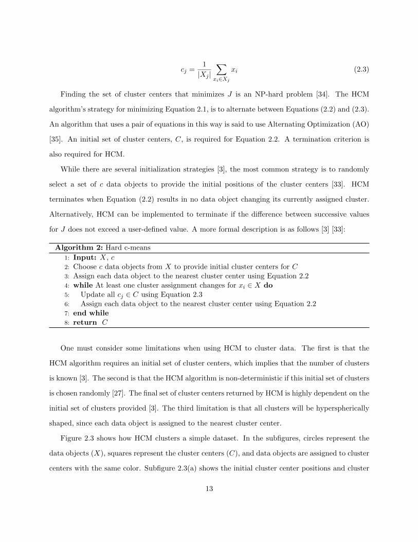
Figure 2.3 shows how HCM clusters a simple dataset. In the subfigures, circles represent the
data objects (X), squares represent the cluster centers (C), and data objects are assigned to cluster
centers with the same color. Subfigure 2.3(a) shows the initial cluster center positions and cluster
13
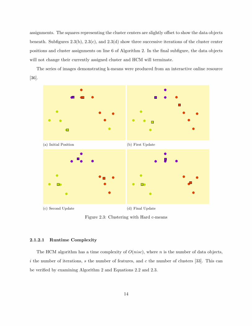
assignments. The squares representing the cluster centers are slightly offset to show the data objects
beneath. Subfigures 2.3(b), 2.3(c), and 2.3(d) show three successive iterations of the cluster center
positions and cluster assignments on line 6 of Algorithm 2. In the final subfigure, the data objects
will not change their currently assigned cluster and HCM will terminate.
The series of images demonstrating k-means were produced from an interactive online resource
[36].
(a) Initial Position (b) First Update
(c) Second Update (d) Final Update
Figure 2.3: Clustering with Hard c-means
2.1.2.1 Runtime Complexity
The HCM algorithm has a time complexity of O(nisc), where n is the number of data objects,
i the number of iterations, s the number of features, and c the number of clusters [33]. This can
be verified by examining Algorithm 2 and Equations 2.2 and 2.3.
14
Equation 2.2 is calculated on line 3 of Algorithm 2. This equation requires a comparison of the
squared distance of every data object to every cluster. The distance calculation requires O(s) time,
and the distance is calculated O(nc) times, for an overall time complexity of O(nsc).
Equation 2.3 is calculated on line 5 of Algorithm 2. This equation finds the average position of
the data objects assigned to each respective cluster. This can be implemented in O(ns) time. On
line 6, Equation 2.2 is calculated again.
Lines 5 and 6 of Algorithm 2 are executed once per iteration, i, until HCM terminates. The
total time complexity (T ) is therefore:
T = O(nsc) + i× (O(ns) +O(nsc))
= O(nsc) +O(nis) +O(nisc)
= O(nisc)
2.1.3 Density Based Spatial Clustering of Applications with Noise (DBSCAN)
DBSCAN is a density-based clustering algorithm, first published in 1996 [24]. Its similarity to
the earlier Jarvis-Patrick algorithm [37] and Parzen window density estimation [38] was noted by
Jain [5].
Conceptually, DBSCAN works as follows. An s-dimension space is defined by the features of
the data objects in a dataset (X). DBSCAN partitions this space into two types of regions, dense
regions considered part of a cluster and sparse regions not considered part of a cluster. Data objects
in the former region are assigned to a cluster, whereas any data objects in the latter region are
considered to be noise. Data objects in a contiguous region of “dense” space are assigned to the
same cluster.
DBSCAN then overcomes the limitations of the distance-based HCM algorithm described in
Section 2.1.2, namely that the: (1) number of clusters must be known in advance, (2) clusters are
hyperspherical, and (3) all data objects must belong to a cluster [21].
15

The local density at each data object is assessed using two parameters, ε (distance) and MinPts
(a lower bound on the minimum number of points, i.e., data objects). A single data object is
considered a “core point” if it is located within ε distance of at least MinPts data objects. All
data objects within ε distance of a core point are considered members of its cluster [21].
Clusters are created from multiple core points located within ε distance from each other. Other
non-core data objects within ε distance of a core point are assigned to that core point’s cluster.
These non-core data objects are called “border points.” As a result, large, irregularly shaped
clusters can be found. As mentioned above, data objects not assigned to a cluster are considered
noise [21].
The original presentation of DBSCAN, presented below as Algorithm 3, formally defines a
number of terms to clarify how the algorithm works [24]:
1. ε Neighborhood (Nε(xi)): The set of data objects within distance ε of data object xi.
2. Core Point: A data object, xi, where |Nε(xi)| ≥MinPts.
3. Border Point: A data object, xi, where |Nε(xi)| < MinPts, xi ∈ Nε(xj) and xj is a core
point.
4. Directly density-reachable: Data object, xi, is directly density-reachable from xj if xi ∈
Nε(xj) and xj is a core point.
5. Density-reachable: Data object, xi, is density-reachable from xj if there is a chain of directly
density-reachable core points between them.
6. Density-connected: Two data objects, xi and xj , are density-connected if both are density-
reachable to some data object xk.
When a core point, xi, not assigned to a cluster is identified on line 12, the algorithm discovers
all data objects directly density-reachable from xi. Subsequently, a recursive call of the Function
ExpandCluster on line 17 allows DBSCAN to find all objects density-reachable from the original
core point. Line 16 ensures the same cluster assignments both for border points and core points.
16

Algorithm 3: DBSCAN
1: Input: X, ε, MinPts2: Assign each data object in X a cluster ID number = 0 (xi.id = 0)3: ClustId = 14: for i = 1 to n do5: if xi.id = 0 then6: ExpandCluster(xi)7: end if8: end for
9: Function ExpandCluster(xi)10: if |Nε(xi)| < MinPts then {xi is not a core point}11: return12: else {xi is a core point}13: xi.id = ClustId14: C = Nε(xi)15: for all xj ∈ C do {xj is a member of xi’s cluster}16: xj .id = ClustId17: ExpandCluster(xj)18: end for19: ClustId = ClustId+ 120: return21: end if
where:X is a dataset consisting of n data objects.ε is a distance.MinPts is an integer.xi is the ith data object in X.C is a set of data objects.A ClusterID = 0 signifies the data object is NOISE.
DBSCAN requires two parameters, ε and MinPts, which define the threshold density for a
cluster. These values can be set empirically. Ester provides a method to set them that works well
in low dimensions [24].
2.1.3.1 Runtime Complexity
A naive implementation of DBSCAN has a runtime complexity of O(n2). Discovery of all data
objects in Nε(xi) requires calculating the distance between xi and ∀xj ∈ X. This step, which
17
occurs on line 10 of Algorithm 3, has a time complexity O(n) and is executed O(n) times (line 4
of Algorithm 3).
If the dataset were sorted into a structure such as an R* tree [39], the discovery of all data
objects in Nε(xi) would have an average runtime complexity of O(log(n)). If this precondition is
met, DBSCAN has a runtime complexity of O(n log(n))
2.2 Algorithms Based on Fuzzy Sets
2.2.1 Fuzzy Sets and Logic
The clustering algorithms discussed in Section 2.1 are based on classical set theory. These
algorithms produce a crisp partition that assigned data objects to a single cluster. A crisp partition
can be expressed as a binary membership matrix, U , where uik ∈ {0, 1} refers to the membership
value of the kth data object, xk, in the ith cluster.
In contrast, fuzzy set theory allows an object to have varying grades of membership in a set [40].
When fuzzy sets are used in a clustering algorithm, a data object can have a grade of membership
in multiple clusters [21]. A fuzzy clustering algorithm produces a fuzzy partition which can also be
expressed by a membership matrix, U . The grade of membership of a data object k in cluster i is
uik. This is subject to the following constraints [41] [22]:
uik ∈ [0, 1], 1 ≤ i ≤ c, 1 ≤ k ≤ n (2.4)
c∑i=1
uik = 1, 1 ≤ k ≤ n (2.5)
n∑k=1
uik > 0, 1 ≤ i ≤ c (2.6)
where n is the number of data objects and c is the number of clusters.
Fuzzy approaches have been successfully integrated in many clustering algorithms [32] [42] [43]
[44] [45]. Three such applications are discussed in this section.
18
2.2.2 Fuzzy c-means (FCM)
The Fuzzy c-means (FCM) algorithm, developed by Bezdek [41], is based on earlier work by
Ruspini and Dunn [28] [5]. As the name suggests, it is a fuzzy variant of HCM.
FCM produces a set of c cluster centers by approximately minimizing the objective function
that calculates the within-group sum of squared distances from each data object to each cluster
center. FCM alternates between calculating optimal cluster centers, given the membership values
of each data object, and calculating membership values, given the cluster centers [22]. If data
objects are defined as feature vectors, xk in Rs, the objective function (Jm) is expressed as [23]:
Jm(U, V ) =
c∑i=1
n∑k=1
umikDik(xk, vi) (2.7)
The functions for determining optimal membership values and optimal cluster centers are derived
from Equation 2.7 using Lagrange multipliers [41]:
uik =Dik(xk, vi)
11−m∑c
j=1Djk(xk, vj)1
1−m
(2.8)
vi =
∑nj=1(uij)
mxj∑nj=1(uij)
m(2.9)
where:
X is a dataset where n = |X|, and xi is the ith data object.
m > 1 controls how fuzzy the clusters are.
c is the number of clusters.
U is the membership matrix; uik refers to the membership value of the kth data element (xk)
for the ith cluster.
V is the set of cluster centers; vi is the ith cluster center.
Dik(xk, vi) is the squared distance between the kth data object and ith cluster center; any inner
product induced distance metric can be used (e.g. Euclidean).
19
There are implementation options. The U or V matrices may be initialized with any valid set of
values. Typically, the uik are initialized with a set of values adhering to (2.4) to (2.6) or each vi is
set to equal the position of a randomly selected data object in X. The FCM algorithm terminates
when the difference between successive membership matrices or sets of cluster centers does not
exceed a given parameter ε [22]. Algorithm 4 describes the implementation used in this research.
Algorithm 4: Fuzzy c-means
1: Input: X, c, m, ε2: Choose c data objects from X to provide initial positions for V3: Assign initial cluster membership values using Equation 2.8.4: maxChange = 1 + ε5: while maxChange > ε do6: Uprev = U7: Update all vi ∈ V using Equation 2.9.8: Reassign cluster memberships to each data object using Equation 2.8.9: maxChange = calcMaxChange(U,Uprev)
10: end while11: return U, V
The function calcMaxChange(U,Uprev) returns the maximum difference in cluster membership
(uik) across two iterations.
2.2.2.1 Runtime Complexity
A literal implementation of the FCM algorithm has an expected runtime complexity of O(nisc2)
[46], where n is the number of data objects, c the number of clusters, s the dimension of the data,
and i the number of iterations. An optimization proposed by Kolen and Hutcheson [47] reduces
the runtime to O(nisc). The remainder of this work uses Kolen’s optimization. For details, see [47]
and Section A.2.3.
2.2.3 Fuzzy c-medoids (FCMdd)
The HCM and FCM algorithms assume that the data objects are represented by numeric feature
vectors. Both algorithms produce cluster centers located in Rs, the feature space of the dataset.
20
Not all datasets, however, consist of data objects represented by feature vectors. Relational
data objects, as opposed to numeric (i.e., object) data, do not have a representation in Rs [48].
For relational data, a measure for similarity or dissimilarity between a pair of data objects can be
defined. A dissimilarity coefficient, ρ(xi, xj), as described in Section 2.1.1, is typically used.
Single Linkage and DBSCAN do not produce cluster centers in Rs. They therefore can produce
clusters from either numeric or relational data. Single Linkage requires no modification to do so.
DBSCAN requires that “distance” be replaced with ρ and that the parameter ε be appropriately
set.
HCM and FCM require modification to accept relational data. Conceptually, HCM and FCM
both seek to minimize an objective function based on the total squared error of a partition of the
data. When using relational data, minimization of such an objective function is still possible.
Hathaway modified Equation 2.7 to accommodate relational data [48]. This modification sub-
stituted a mean cluster membership vector for cluster centers. Versions include Relational Hard
c-means (RHCM), Relational Fuzzy c-means (RFCM), and Non-Euclidean RFCM (NERF) [48]
[49].
One can also select representative data objects from the dataset as cluster centers. When
discussing clustering algorithms, such representative objects are referred to as medoids. In the field
of Operations Research, variations of this problem are known as the facility location problem and
k-median problem [50] [28].
Crisp set versions of a “Hard c-medoid” algorithm include Partitioning Around Medoids (PAM),
and Clustering Large Applications (CLARA) [51] [28]. Its fuzzy set version is Fuzzy c-medoids
(FCMdd) [44]. Krishnapuram originally developed the FCMdd algorithm to cluster textual data
[52] [44].
FCMdd minimizes the objective function Jm.
Jm(V,X) =n∑i=1
c∑j=1
umijρ(xi, vj) (2.10)
21
where:
X is a dataset where n = |X|, and xi is the ith data object.
m > 1 is the “fuzzifier.”
c is the number of clusters.
U is the membership matrix; uij refers to the membership value of the ith data element (xi) for
the jth cluster.
V is the set of cluster centers; vj is the jth cluster center.
ρ(xi, vj) is the dissimilarity between the ith data object and jth cluster center.
The same membership function used for FCM can be used for FCMdd if the squared distance
is replaced with the dissimilarity. Although other membership functions can be used [44], I imple-
mented Equation 2.11 for the work described here.
uij =ρ(xi, vj)
11−m∑c
k=1 ρ(xi, vk)1
1−m
(2.11)
Like FCM, FCMdd is provided an initial set of medoids, V . Note that unlike FCM, the medoids
are always data objects, xi. It then alternates between calculating the membership matrix, U (based
on the values in V ), and calculating new medoids, V (based on the values in U), until a termination
criterion is met.
Unfortunately, no equation is provided for the optimization of the medoids. FCMdd is not a
true alternating optimization algorithm, and a Lagrangian “hill-climbing” formula cannot be used
as with FCM [41] [44].
Selection of the optimal c medoids that reduce the value of Jm for the current values in U would
require testing(nc
)combinations. Clearly, this is intractable, so a heuristic proposed by Fu [53]
is used. The heuristic keeps all but one vj ∈ V fixed, and it evaluates the remaining n − c data
objects in xi ∈ X. If there are any xi, if substituted for vj in Equation 2.10, that would result in
a lower value for Jm, the xi that would minimize Jm replaces vj in V . Each vj ∈ V is considered
per iteration.
22
FCMdd’s initialization and termination criterion remain to be discussed. Initialization of
FCMdd requires the selection of c medoids to populate V . The most obvious technique is to
select c data objects randomly. Empirically, Krishnapuram noted that FCMdd often would become
stuck in local extrema if this technique was used [44].
An alternative technique is to randomly select a single data object, xi, to insert into V . Then,
the data object, xj ∈ X, with the greatest dissimilarity from xi should be selected and placed
into V . For the remaining c − 2 medoids, each successive data object, xk ∈ X, with the greatest
sum of dissimilarity to all objects currently in V will be selected. This technique, described in [52]
as “Initialization III,” experimentally produces higher-quality partitions than those produced by
random selection. Initialization III was used in research.
Similarly to HCM, the FCMdd algorithm terminates when V remains unchanged between up-
dates to U . FCMdd also terminates if it reaches a maximum number of iterations (MAX ITER).
In the implementation for research, MAX ITER was hard-coded to equal 100. It was noted in [54]
that the algorithm can get stuck in a cycle where the medoids in V alternate between two assign-
ments until MAX ITER is reached. This condition was tested for also. If V , in iteration i, had
the same assignments as V , in iteration i+ 2, the algorithm terminated. A single test is sufficient,
because the update process is deterministic for a given dataset and starting set of medoids.
The formal description of FCMdd as listed in Algorithm 5 is slightly modified from its original
publication [44].
2.2.3.1 Runtime Complexity
Krishnapuram reported the runtime complexity of FCMdd as O(n2) [52]. If the number of
iterations, i, and the number of clusters, c, are considered, the runtime complexity will be higher.
An in-depth analysis of runtime complexity follows. One assumption made in the analysis is that
the dissimilarity between two data objects can be calculated in constant time.
On line 2 of Algorithm 5, the initial set of medoids is selected. This initialization technique has
a runtime complexity of O(nc2) [52]. The while statement on line 5 is executed i times. Within the
while statement, the membership matrix is updated on line 7. This step has a runtime complexity
23
Algorithm 5: Fuzzy c-medoids
1: Input: X, c, m2: Select c data objects from X to provide an initial set of medoids V .3: Set Vold = NULL4: Set ITER = 05: while (Vold 6= V and ITER < MAX ITER) do6: Vold = V7: Update membership matrix U using Equation 2.118: for j = 1 to c do9: p = argmin(1≤k≤n)
∑ni=1 u
mijρ(xk, xi)
10: vj = xp11: end for12: ITER = ITER+ 113: end while14: return C
of O(nc). Also within the while statement, on line 9, an estimate is calculated of the impact of
changing vi. This step has a runtime complexity of O(n2), is within the for loop on line 8, and is
executed c times. The total runtime complexity (T ) is therefore:
T = O(nc2) + i× (O(nc) + c×O(n2))
= O(nc2) +O(nci) +O(n2ci)
= O(n2ci)
2.2.4 Fuzzy Neighborhood DBSCAN (FN-DBSCAN)
Nasibov and Ulutagay modified the DBSCAN algorithm to integrate fuzzy set theory [45].
Fuzzy Neighborhood Density-Based Spatial Clustering of Applications with Noise (FN-DBSCAN)
employs a fuzzy neighborhood function rather than a crisp set definition to assess density [55]. FN-
DBSCAN repairs one of DBSCAN’s flaws [21]. Since DBSCAN uses a crisp definition for density,
a data object, xp, at nearly ε distance from a group of data objects, is assigned the same density
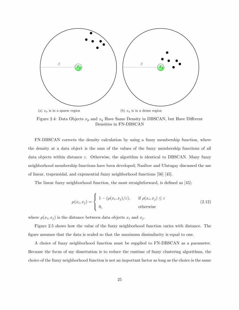
as a data object, xq, in close proximity to a similar group of data objects (Figure 2.4 ).
24
xpε
(a) xp is in a sparse region
xqε
(b) xq is in a dense region
Figure 2.4: Data Objects xp and xq Have Same Density in DBSCAN, but Have DifferentDensities in FN-DBSCAN
FN-DBSCAN corrects the density calculation by using a fuzzy membership function, where
the density at a data object is the sum of the values of the fuzzy membership functions of all
data objects within distance ε. Otherwise, the algorithm is identical to DBSCAN. Many fuzzy
neighborhood membership functions have been developed; Nasibov and Ulutagay discussed the use
of linear, trapezoidal, and exponential fuzzy neighborhood functions [56] [45].
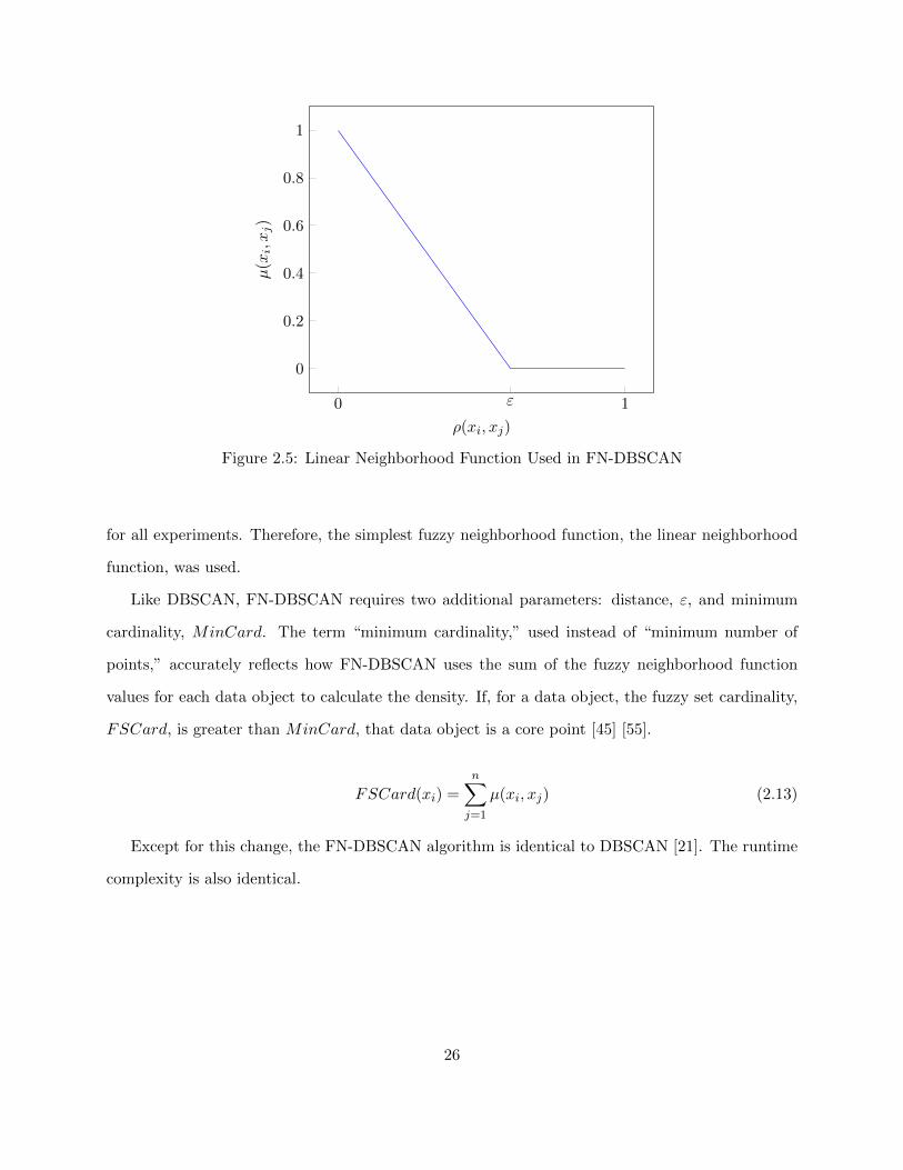
The linear fuzzy neighborhood function, the most straightforward, is defined as [45]:
µ(xi, xj) =
1− (ρ(xi, xj)/ε), if ρ(xi, xj) ≤ ε
0, otherwise(2.12)
where ρ(xi, xj) is the distance between data objects xi and xj .
Figure 2.5 shows how the value of the fuzzy neighborhood function varies with distance. The
figure assumes that the data is scaled so that the maximum dissimilarity is equal to one.
A choice of fuzzy neighborhood function must be supplied to FN-DBSCAN as a parameter.
Because the focus of my dissertation is to reduce the runtime of fuzzy clustering algorithms, the
choice of the fuzzy neighborhood function is not an important factor as long as the choice is the same
25
0 ε 1
0
0.2
0.4
0.6
0.8
1
ρ(xi, xj)
µ(xi,xj)
Figure 2.5: Linear Neighborhood Function Used in FN-DBSCAN
for all experiments. Therefore, the simplest fuzzy neighborhood function, the linear neighborhood
function, was used.
Like DBSCAN, FN-DBSCAN requires two additional parameters: distance, ε, and minimum
cardinality, MinCard. The term “minimum cardinality,” used instead of “minimum number of
points,” accurately reflects how FN-DBSCAN uses the sum of the fuzzy neighborhood function
values for each data object to calculate the density. If, for a data object, the fuzzy set cardinality,
FSCard, is greater than MinCard, that data object is a core point [45] [55].
FSCard(xi) =
n∑j=1
µ(xi, xj) (2.13)
Except for this change, the FN-DBSCAN algorithm is identical to DBSCAN [21]. The runtime
complexity is also identical.
26
2.3 Accelerated Clustering Algorithms
2.3.1 Significant Work Related to Acceleration
The focus of my dissertation is to reduce the runtime of fuzzy clustering algorithms while
keeping quality loss to a minimum. As clustering algorithm research has has intense focus for five
decades, there has been and continues to be much interest in accelerating clustering algorithms.
This section describes significant work relevant to the methods used and experiments described in
this dissertation. Accelerated algorithms, used for experiments in the research or related to this
work, are described in the sections below.
A literal implementation of the FCM algorithm, as described in Section 2.2.2.1, has an expected
runtime complexity of O(nisc2), where n is the number of data objects, c the number of clusters,
s the number the data features, and i the number of iterations. As previously mentioned, it is
possible to reduce the runtime to O(nisc) with the optimization proposed by Kolen and Hutcheson
[47].
Given a dataset with c natural clusters, an FCM variant can be accelerated further by reducing
n, s, or i. There are techniques for reducing the number of features, s, but many of these techniques
preprocess the data rather than being integrated into the algorithm itself [57] [58]. An alternative
technique, subspace clustering, looks for clusters using a subset of the available features [59] [60].
Each cluster found can use a different subset of the available features. This line of research, however,
was not pursued. My dissertation focused on techniques that reduce the amount of data used, n,
and the number of iterations, i.
Algorithms such as FCM, designed to minimize an objective function value, have shorter run-
times if their initial cluster centers are close to the final solution. The shorter runtime is due to a
reduction in iterations before termination. Bradley and Fayyad [61] investigated the effects of an
improved starting position for HCM. A better start position reduced the runtime, but their study
was focused on quality, not speed.
Processing a small data sample to obtain an improved initial starting point for FCM has been
investigated. Cheng describes an iterative process to develop a “good” starting point [62]. This
27
method, Multistage Random Sampling FCM (mrFCM), consists of two parts. The first part pro-
gressively samples the dataset, improving the starting clusters until a termination criterion is met.
Then mrFCM uses these starting clusters to initialize FCM on the full dataset.
Similarly, Altman uses FCM to obtain a set of cluster centers from a small sample of data
objects. These cluster centers are used to initialize the membership matrix, U , before clustering
the full dataset with FCM [63].
In Partition Simplification FCM (psFCM), Hung and Yang [64] partition the data using a k-d
tree to obtain a simplified dataset, which in turn is used as a subsample to estimate the position
of the cluster centers. The resulting estimate is used to initialize FCM on the full dataset.
The Single Pass FCM (SPFCM) algorithm, discussed in Section 2.3.2, incrementally clusters
the data and passes on the cluster centers from each increment as an initialization for the next [46].
Online FCM (OFCM), discussed in Section 2.3.3, follows a similar strategy [65].
Provost presented an overview of the progressive sampling technique in the context of induc-
tion (a.k.a. classification) algorithms [66]. Progressive sampling uses an initial subsample to form
a classifier, which is tested on labeled data. The subsample progressively increases in size arith-
metically or geometrically, creating a new classifier each time it grows. When the accuracy of the
classifier ceases to improve significantly when compared to the previous sample, the addition of
data is terminated.
Progressive sampling techniques have been applied to clustering problems. These techniques
accelerate a clustering algorithm by reducing the number of data objects, n, that are clustered.
Domingos and Hulten [67] used Hoeffding bounds in a progressive sampling technique both to
estimate the initial sample size and to estimate the sufficiency of the sample size at any point in the
progression. The technique, developed for HCM, assumes that each data object has membership
in only one cluster. It calculates the worst-case bounds, and the sample sizes are typically large.
Pal and Bezdek [68] and Wang et al. [69] used progressive sampling to select a subsample
representative of the dataset. They used a divergence test to assess whether the subsample matched
the distribution of the dataset. If the test failed, progressively larger subsamples were taken until
28
the test passed. Finally a clustering algorithm was run on the chosen subsample. This technique,
extensible Fast FCM (eFFCM), is discussed in detail in Section 2.3.4.
A very simple way to reduce n is to select a sample of the dataset and to apply the clustering
algorithm to the sample. Havens et al. [16] use this technique in the random sampling plus extension
FCM (rseFCM) algorithm, which is discussed further in Section 2.3.5
2.3.1.1 Relational Clustering
Fewer techniques exist for accelerating relational clustering algorithms.
Clustering Large Applications (CLARA) accelerates the PAM algorithm by repetitively sam-
pling the dataset [28]. Each sample is clustered using PAM, and the clustering solution is extended
to the entire dataset. The clustering solution with the lowest (best) objective function is returned.
The sample size and number of samples taken are user-determined.
An optimization to FCMdd is Linearized Fuzzy C-Medoids (LFCMdd). This accelerated variant,
as the name suggests, reduces the runtime complexity to be linear with respect the number of data
objects, i.e., O(nci). LFCMdd considers only the data objects with the highest membership values
as candidates to update the current set of cluster centers [44].
Labroche directly adapted SPFCM and OFCM to use FCMdd as the base algorithm [54]. These
accelerated algorithms, History Based Online Fuzzy C-Medoids (HOFCMD) and Online Fuzzy C-
Medoids (OFCMD), are otherwise identical to SPFCM and OFCM respectively.
Bezdek (et al.) created an accelerated, relational version of eFFCM called extended non-
Euclidean relational fuzzy c-means (eNERF) [70]. The eFFCM algorithm, described in detail
in Section 2.3.4, depends on the existence of features from which to select a sample of the data.
These features, of course, do not exist in relational data. To solve this problem, eNERF considers
relations between data objects rather than features, and then selects a subset of relations that are
dissimilar to each other. The eNERF algorithm otherwise uses a strategy similar to that of eFFCM.
29
2.3.2 Single Pass Fuzzy c-means (SPFCM)
Prodip Hore developed SPFCM as part of his dissertation research [71]. The SPFCM algorithm
breaks the dataset into equally sized “partial data accesses” (PDA). A user-provided parameter,
“fractional PDA” (fPDA ≤ 0.5), defines the PDA size as fPDA × n where n equals the total
number of data objects. SPFCM incrementally processes the entire dataset one PDA at a time.
Each PDA is processed by a weighted version of FCM, aptly named Weighted FCM (WFCM). In
the WFCM algorithm, each data object, xi, has an associated weight, wi. The objective function
and cluster center calculation from Section 2.2.2 are modified as follows [46] [11]:
Jmw(U, V ) =
c∑i=1
n∑k=1
umikwkDik(xk, vi) (2.14)
vi =
∑nj=1wj(uij)
mxj∑nj=1wj(uij)
m(2.15)
where wi is a non-zero weight for a data object.
Data objects are initially given a weight of 1. After the cluster centers, vi ∈ V , are calculated
from the first PDA, the cluster centers are assigned weights using the following Equation [11]:
w′i =n∑j=1
(uij)wj , 1 ≤ i ≤ c (2.16)
SPFCM uses weighted cluster centers as representative objects. These weighted cluster centers
represent the partition information from the first PDA. The c cluster centers are added as additional
data examples to the second PDA, which is then clustered by WFCM. The positions of the cluster
centers calculated from the first PDA are used as the initial values for V in the second PDA. This
process is repeated until all PDAs have been clustered. SPFCM returns as a final solution the set
of cluster centers from the last PDA.
The SPFCM algorithm assumes that the data objects in the dataset have been randomly or-
dered. Datasets with some sort of inherent order in the data, typical in images, can result in PDAs
30
significantly different with respect to the overall distribution. The implementation used in this
research randomizes the data prior to processing.
2.3.2.1 Runtime Complexity
The runtime complexity of FCM is O(nisc) (Section 2.2.2.1). Note that the runtime complexity
is linear with respect to n, the number of data objects. The SPFCM algorithm also processes the
entire dataset, albeit incrementally, so a cursory analysis of the runtime complexity would also
yield O(nisc).
Hore reports that SPFCM had a shorter runtime than FCM on the datasets he tested [46]. Hore
identified the cause: after the first PDA had been clustered, the derived cluster centers were used
to initialize V in the subsequent PDA. Initial cluster centers closer to the optimal cluster centers
allow the algorithms in the HCM family to terminate with fewer iterations [61].
Reviewing complexity analysis in a similar manner as [46] [71], the following notation is used:
n is the size of the dataset.
p is the PDA value as a fraction (fPDA).
d = 1p is the number of partial data accesses required.
ij : is the number of iterations in the jth PDA.
Tj = O(pnijsc) runtime complexity for the jth PDA
i = p∑d
j=1 ij average number of iterations per PDA
T = O(∑d
j=1 pnijsc) total runtime complexity for SPFCM
T = O(nisc) substituting i into expression for T
(2.17)
The runtime complexity of SPFCM is O(nisc). When SPFCM clusters a dataset it has a shorter
runtime compared with FCM because typically, i < i.
2.3.3 Online Fuzzy c-means (OFCM)
Prodip Hore also developed OFCM as part of his dissertation research [71]. OFCM breaks the
dataset into PDAs and clusters each PDA, in the same manner as SPFCM. The OFCM algorithm
31
produces a set of cluster centers from each PDA and, using Equation 2.16, calculates their weights.
These weighted cluster centers represent the partition information in each PDA.
The OFCM and SPFCM algorithms, though similar, have one major difference [11]. Unlike
SPFCM, OFCM saves each set of weighted cluster centers, instead of adding them to the subsequent
PDA. After all PDAs have been clustered, the saved sets of weighted cluster centers from each PDA
are combined into one dataset. Then, WFCM clusters this combined dataset. OFCM returns as a
final solution the set of cluster centers from the combined dataset.
An advantage of OFCM is that the processing of a dataset can be separated over distance
or time. In these cases, the initial set of cluster centers is chosen locally by random selection.
Alternatively, cluster centers from a previous PDA can be used as initial cluster centers. While the
latter strategy matches the original implementation of the algorithm [65], a PDA not representative
of the entire dataset will provide a poor initial set of starting clusters. OFCM does not assume that
the dataset is in random order. In this dissertation, except where explicitly noted, the datasets
clustered by OFCM were not randomized.
The runtime complexity analysis of OFCM is fundamentally the same as the analysis in Section
2.3.2.1.
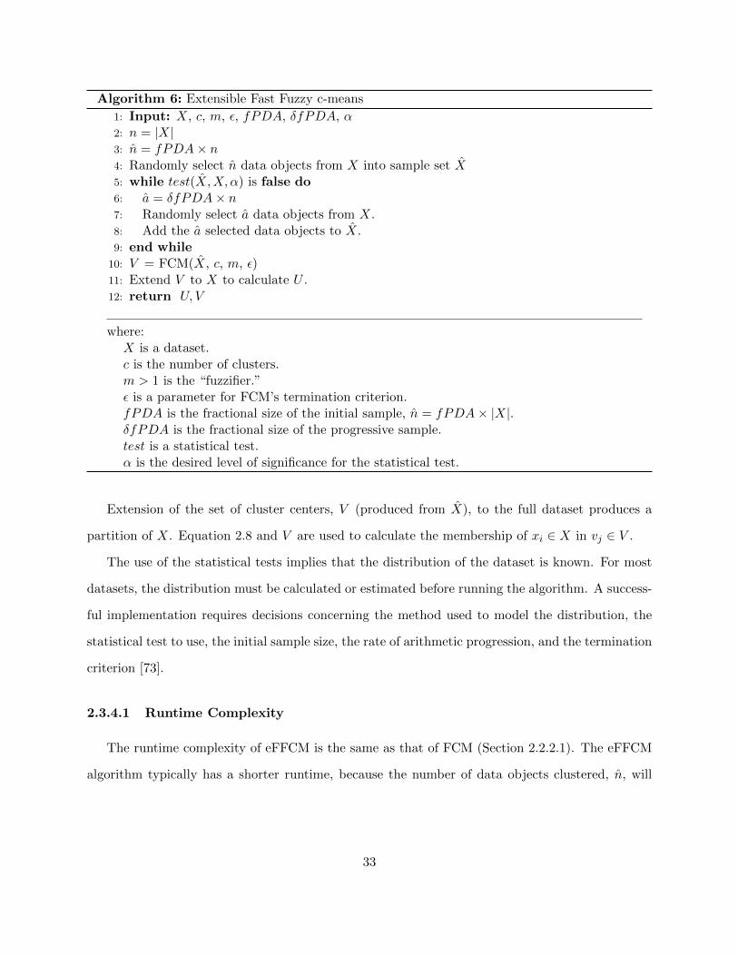
2.3.4 Extensible Fast Fuzzy c-means (eFFCM)
The eFFCM algorithm clusters a statistically significant sample, X, as opposed to the full
dataset, X. Statistical significance is tested for by comparing the distribution of the sample with
the distribution of X using the Chi-square (χ2) statistic or Kullback-Leibler divergence. It is
formally presented as Algorithm 6.
If the initial sample fails testing, additional data is progressively added to the sample and the
new sample is tested. This procedure is repeated until a sample has passed the statistical test
[68] [72]. The size of each additional subsample is constant; therefore the sampling procedure uses
progression with an arithmetic schedule [66]. The final statistically significant sample, X, is then
clustered by FCM to obtain a set of cluster centers.
32
Algorithm 6: Extensible Fast Fuzzy c-means
1: Input: X, c, m, ε, fPDA, δfPDA, α2: n = |X|3: n = fPDA× n4: Randomly select n data objects from X into sample set X5: while test(X,X, α) is false do6: a = δfPDA× n7: Randomly select a data objects from X.8: Add the a selected data objects to X.9: end while
10: V = FCM(X, c, m, ε)11: Extend V to X to calculate U .12: return U, V
where:X is a dataset.c is the number of clusters.m > 1 is the “fuzzifier.”ε is a parameter for FCM’s termination criterion.fPDA is the fractional size of the initial sample, n = fPDA× |X|.δfPDA is the fractional size of the progressive sample.test is a statistical test.α is the desired level of significance for the statistical test.
Extension of the set of cluster centers, V (produced from X), to the full dataset produces a
partition of X. Equation 2.8 and V are used to calculate the membership of xi ∈ X in vj ∈ V .
The use of the statistical tests implies that the distribution of the dataset is known. For most
datasets, the distribution must be calculated or estimated before running the algorithm. A success-
ful implementation requires decisions concerning the method used to model the distribution, the
statistical test to use, the initial sample size, the rate of arithmetic progression, and the termination
criterion [73].
2.3.4.1 Runtime Complexity
The runtime complexity of eFFCM is the same as that of FCM (Section 2.2.2.1). The eFFCM
algorithm typically has a shorter runtime, because the number of data objects clustered, n, will
33

typically be less than n, the number of data objects in the full dataset. This makes eFFCM’s
runtime O(nisc).
Selection of the sample and extension of the solution to the full dataset are separate steps.
Their runtime complexities must be added to those of eFFCM. It takes O(n) time to model the
distribution and to obtain random samples. Extending the solution using Equation 2.8 has a time
complexity of O(nsc). This makes the total runtime O(nisc) +O(nsc) +O(n).
If one assumes that ni ≥ n, the runtime complexity for eFFCM remains O(nisc). Experimental
results, discussed in Section 4.4, show that this is a reasonable assumption. As a practical concern,
the sampling and extension do add significant overhead to an implementation of the algorithm.
2.3.5 Random Sampling Plus Extension Fuzzy c-means (rseFCM)
This algorithm uses FCM to cluster a random sample, X, of the dataset, X. The size of X
is a user-defined parameter [16]. Using Equation 2.8, a complete partition of X is produced by
extending the set of cluster centers produced from X to the full dataset.
If n = |X| is substituted for n, the runtime complexity of rseFCM will be the same as that of
FCM (Section 2.2.2.1). Randomly selecting X takes O(n) time. Thus, the total runtime is O(nisc).
2.3.6 Density Based Distributed Clustering (DBDC)
Density Based Distributed Clustering (DBDC) is a distributed, scalable version of DBSCAN
that can provide a speedup over DBSCAN [74] [21]. The DBDC algorithm assumes the existence
of multiple sites with local datasets. The goal of the algorithm is to cluster the union of all the
local datasets. Conceptually, this has the same structure as any accelerated algorithm that breaks
a large dataset into smaller subsets.
DBDC uses DBSCAN to cluster the local datasets at each site. Each local clustering solution is
represented by a set of data objects, the “specific core points,” and a set of distances, the “specific
ε-ranges.” The set of specific core points is a subset of the core points defined by DBSCAN such
that none of the specific core points are within ε distance of each other. Each specific core point is
assigned a specific ε-range to define the extent of the search space volume it represents.
34

Each local set of specific core points and specific ε-ranges are combined to create a global
dataset. DBSCAN clusters this global dataset, with MinPts set to 2. The rationale for MinPts’s
setting is that the global dataset only consists of core points. Thus, two core points define a larger
cluster if their distance apart is ε or less.
The user sets the ε parameter. The authors of the algorithm suggested using the largest specific
ε-range for ε, but they admit that this setting might not work for all datasets. The value for ε
would need to exceed the specific ε-range for datasets in which the specific core points for a cluster
only exist in one local model. Otherwise, these specific core points for this cluster would be greater
than ε apart in the global dataset and would not define a cluster.
2.3.7 Scalable DBDC (SDBDC)
The Scalable DBDC (SDBDC) algorithm was designed to repair flaws in DBDC [75]. In addition
to the difficulty in setting epsilon (described above), DBDC ignores “noise” at each local site that
could potentially define a cluster when combined globally.
SDBDC makes the same assumptions as DBDC but uses a different criterion to select represen-
tative data objects at each local site. DBSCAN clusters the data objects at each local site. Fuzzy
logic is not explicitly mentioned in [75], but a linear fuzzy membership function does calculate the
sum of the membership functions within ε distance of each data object. This sum is referred to as
a “representation quality.”
The representation qualities for each data object are listed in descending order. The data object
with the highest representation quality is selected as a representative object and removed from the
list. The representation quality is recalculated for each data object remaining in the list, and the
list is resorted. This process repeats until enough representative data objects have been selected.
Januzac (et al.) designed SDBDC to allow the user to determine an acceptable trade-off between
speedup and quality of results. Thus, the actual number of representative objects from each local
site is user-configured.
35
Additional data is recorded for each representative data object: the number of data objects
“covered” by each representative object and the distance to the farthest data object it “covers.”
These are called the “covering number” and the “covering radius.”
The representative data objects from each local site are combined globally, and a modified
version of DBSCAN clusters the data. The global algorithm is more complex, since it considers the
“covering number” as a weight and modifies the ε parameter with the “covering radius” separately
for each representative data object.
2.4 Evaluation Metrics
This section presents the evaluation metrics used in this dissertation and related works.
The term, “quality”, is frequently used when evaluating experimental results. Quality, properly
defined, refers to “the degree of excellence which a thing possesses” [76]. In this dissertation, quality
is only used to describe the results (cluster centers, partition, etc.) obtained from the clustering
algorithm. The degree to which the accelerated algorithm succeeds at its task is referred to as
speedup, never quality.
Quality can only be measured by some objective function. The FCM family of algorithms seeks
to reduce an objective function. We compare the final objective function values of two algorithms
using the DQRm% metric which is described below.
It is possible for two algorithms to have identical objective function values, but result in different
partitions. So, the second way to evaluate the final partition was to compare the degree to which
the partitions produced by two algorithms differ. Assuming the reference algorithm produces an
ideal partition, what is being measured is the degree to which the competing algorithm is faithful
to the reference. These types of metrics are referred to in this dissertation as “fidelity” metrics.
The term, “fidelity”, is used to differentiate a metric from DQRm. In this research, CC%, DFV%,
and ARI are recorded as fidelity metrics and described below.
36

2.4.1 Relative Speedup (SU)
Because the goal of the dissertation is to develop new methods that reduce the runtime of
clustering algorithms, a metric is necessary to compare competing algorithms. The SU metric
calculates the ratio between the runtimes of two algorithms. If t1 is the runtime of candidate
algorithm 1 and t2 the runtime of the reference algorithm, the speedup of algorithm 1 relative to
algorithm 2, SU12, is:
SU12 =t2t1
(2.18)
For example, if algorithm 1 has a runtime of 150ms and algorithm 2 a runtime of 750ms, the
speedup equals 5. Algorithm 1 is five times as fast as algorithm 2.
2.4.2 Difference in Quality of Objective Function
Many clustering algorithms are designed to minimize the value of a squared error function, also
called the objective function. Minimization of this value is the goal of the HCM algorithm and
its variants, so comparisons using the objective function, Jm, have been employed as a means of
comparing the quality of results of different algorithmic variants [46] [77].
If Jm1 is the objective function value for algorithm 1, and Jm2 the objective function value for
(the reference) algorithm 2, then the percentage difference in quality of algorithm 1 relative to that
of algorithm 2 is:
DQJm% =
(Jm1 − Jm2
Jm2
)× 100 (2.19)
The accelerated algorithms based on FCM (SPFCM, OFCM, eFFCM, rseFCM) use different strate-
gies to sample the dataset. Values of Jm produced by these accelerated algorithms potentially use
different-sized samples and are thereby not comparable. Calculation of DQJm% would require ex-
tension of the clustering solutions to the full dataset in order to obtain membership values (Equation
2.8) so that Jm can be calculated for each algorithm.
37
Fortunately, the objective function Jm (2.7) is mathematically equivalent to a reformulated
optimization criterion (Rm) [78] [77]:
Rm(V ) =
n∑k=1
(c∑i=1
Dik(xk, vi)1
(1−m)
)(1−m)
(2.20)
The Rm calculation is more convenient than Jm because it requires only the original dataset and
the cluster centers. The percentage difference in quality between algorithm 1 and 2 is calculated
as follows [46]:
DQRm% =
(Rm1 −Rm2
Rm2
)× 100 (2.21)
where Rm1 is the reformulated optimization criterion for algorithm 1, and Rm2 for (the reference)
algorithm 2.
2.4.3 Cluster Change Percentage
Clustering algorithms in the HCM family require an initial starting point, typically a starting
set of cluster centers, Vinit. When Vinit is randomly selected over multiple trials, the algorithm
often produces different partitions for every trial. Two trials of a clustering algorithm may have
similar values for Jm but radically different partitions. It is theoretically possible, though unlikely,
for two different partitions to have identical Jm values. So, other metrics are needed that do not
have this problem.
The cluster change percentage, CC%, is a complimentary method of comparing the fidelity
of clustering algorithms. The assigned cluster for each data object in the dataset is compared
between two partitions. An indicator variable, δi, is set to 0 if the cluster assignments are the same
in both partitions, and it is set to 1 if they are different. In the case of fuzzy clustering, the cluster
assignments are “hardened” by assigning each data object to the cluster in which its membership
value, uij , is highest. For a pair of partitions, A and B, the CC% is [77]:
CC%(A,B) =
∑ni=1 δin
× 100 (2.22)
38
This metric requires a method to identify corresponding clusters in partitions A and B. In my
research, the Hungarian Method was used [79].
A small amount of cluster change indicates that the two partitions are very close. When one
partition is from the reference algorithm, a small CC% value signifies that the candidate algorithm
has created a highly similar partition to the original algorithm.
When comparing two or more experiments, each involving multiple trials of clustering algo-
rithms, the use of CC% is straightforward, as long as the data objects have been defined as feature
vectors in Rs. For an algorithm, the averages for the values in V over all experiments can be used
to define the partition. Equation 2.22 can then be used to calculate the CC% between any pair of
algorithms. The fact that the cluster centers have representation in Rs also allows examination of
how the positions of cluster centers in V vary, indicating the consistency of the clustering method
(see Section 2.4.4).
When the algorithms and data are relational, the cluster centers do not have representation in
Rs, and the use of Equation 2.22 is not so straightforward. For instance, if there were 30 trials per
experiment, there would be 30 sets of medoids. It is not possible to average the medoids as if they
were cluster centers and to use the procedure described above.
Within multiple trials of an experiment using a relational algorithm, it is possible to compute
the CC% between any pair of trials. For an experiment consisting of t trials, the average CC%
can be calculated over every pair of trials. This I define as the intraCC%:
intraCC% =1(t2
) t∑i=1
t∑j=i+1
CC%(Ti, Tj) (2.23)
where Ti is the partition from the ith trial.
The CC% can also be calculated between the trials of two experiments with different clustering
algorithms. This I define as the inter CC%:
inter CC% =1
t2
t∑i=1
t∑j=1
CC%(Ti, Tj) (2.24)
39
where the i subscript indicates trials from one algorithm and the j subscript indicates trials from
the other. Equation 2.24 assumes that both experiments have the same number of trials.
2.4.4 Difference in Fidelity of Partitions
As noted in Section 2.4.3, algorithms that randomly select an initial set of cluster centers, Vinit,
could, over many trials, produce a different partition every trial.
Difference in fidelity of partitions (DFV ) compares the variation of the cluster centers (V )
produced by a candidate algorithm to that of a reference algorithm [77]. DFV can be used to
assess the variation that a single algorithm experiences over multiple trials, or it can be used to
compare two different algorithms. DFV is calculated as a percentage:
DFV% =
(∑ti=1
∑cj=1 ||V
′ij − V avgj ||
t×∑c
j=1 ||V avgj ||
)× 100 (2.25)
where:
t: is the number of trials.
V′ij : is the jth cluster center from the ith trial of the candidate algorithm.
V avgj : is the average position the jth cluster center produced by the reference algorithm.
|| · ||: is the length of the vector (·).
The DFV metric provides an indication of a candidate algorithm’s stability, compared either
to itself or to a reference algorithm. It requires a method to identify corresponding cluster centers
across trials. In my research, the Hungarian Method was used [79].
2.4.5 Adjusted Rand Index (ARI)
The Rand Index evaluates the similarity between two partitions [80]. Given two partitions, A
and B, the Rand Index returns a value in the range of 0 to 1; 0 when the partitions are in complete
disagreement, and 1 when the partitions are in complete agreement.
40

The cluster assignments of every possible pair of data objects (xi, xj ∈ X) are used2 to calculate
the Rand Index (RI) [81]:
RI =a+ d
a+ b+ c+ d(2.26)
where:
a - the number of pairs of data objects with the same cluster assignments in both partitions A
and B.
b - the number of pairs of data objects with the same cluster assignments in partition A but
different cluster assignments in partition B.
c - the number of pairs of data objects with different cluster assignments in partition A with
the same cluster assignments in partition B.
d - the number of pairs of data objects with the different cluster assignments in both partitions
A and B.
A difficulty with RI is that it does not take chance into account. If the data objects in both
partitions were assigned clusters randomly, then a number of pairs would coincide purely by chance.
A modified form, the Adjusted Rand Index (ARI), corrects this problem [82]:
ARI =RI − E[RI]
1− E[RI](2.27)
where E[RI] is the expected value of RI if data objects in the partitions are distributed randomly.
ARI returns a value of 1 when the partitions are in complete agreement, 0 when the partitions
return the value expected by chance, and a negative value when the partitions are in greater
disagreement than would be expected by chance.
The Rand Index and ARI can be used to compare the partition of an accelerated (candidate)
algorithm to that of the reference algorithm. The Rand Index and ARI also assume that the
2Given n = |X|, the number of pairs equals(n2
). RI calculation has a time complexity of O(n2) and can be
impractical for very large datasets.
41

clustering is discrete, i.e., hard [80] [82]. For fuzzy clustering, the partitions must be hardened by
assigning each data object to the cluster in which it has the highest membership value [16].
2.4.6 Accuracy
When the actual class labels are available for a test dataset, calculating the percentage accuracy
of a clustering solution is an obvious metric, but somewhat misleading because clustering algorithms
do not optimize accuracy. Each cluster label is associated with a class label and any data object
whose cluster label does not match its associated class is considered inaccurate. Prior to the
calculation, clusters must be aligned to the class labels. In my research, the Hungarian method
was used [79].
2.4.7 Some Statistics
2.4.7.1 Welch’s t-test
This test for significance compares the means of two populations when the numbers of samples
in each population are small and the sample variances cannot be assumed to be equal [83]. The t
statistic and the associated degrees of freedom are calculated as follows [84]:
t =X1 − X2√s21n1
+s22n2
(2.28)
ν =
(s21n1
+s22n2
)2s41
n21(n1−1)
+s42
n22(n2−1)
(2.29)
where:
Xi: is the ith sample mean
si: is the ith sample standard deviation
ni: is the ith sample size
ν : are the degrees of freedom
42

2.4.7.2 Z-test
Mean values and sample standard deviations were calculated for many of the metrics in the
experiments. The z statistic can then be calculated to test for statistical significance in the difference
between mean values produced by two different algorithms [84].
z =(X1)− (X2)√
(σ21/n1) + (σ22/n2)(2.30)
where:
X1 and X2 are mean values from algorithms 1 and 2 respectively.
σ21 and σ22 are samples variances from algorithms 1 and 2 respectively.
n1 and n2 are the metric populations from algorithms 1 and 2 respectively.
The most common test I used was an estimation of whether two mean values were different, i.e.,
a two-tailed test. Using the null hypothesis, H0, that there is no difference between means, and
the alternative hypothesis, H1, that X1 6= X2, if z exceeds the value for the specified confidence
level, H0 must be rejected. Typically, the 95% confidence level is used, in which z = 1.96, and a
calculated value z > 1.96 or z < −1.96 means there is a significant difference.
43
Chapter 3: Datasets
“I don’t know what the best type is, but I know none is bad.” - Lawrence “Yogi” Berra [2]
3.1 About the Datasets
Seventeen original datasets were used in experiments. Eleven datasets were obtained from real-
world data sources, the other six were artificially constructed. An additional six datasets were
derived from subsets of real world datasets, bringing the total number of datasets used to twenty
three.3
The datasets are described in detail in the sections below. Table 3.1 lists the number of data
objects, features and classes for all datasets.
3.2 MRI Datasets
Three datasets used in experiments, MRI016, MRI017, and MRI018, are magnetic resonance
images (MRI) of a normal human brain. Each dataset has approximately four million data objects.
The images were pre-processed to remove non-brain tissue (bone, fat, skin, etc.) and air. The three
data features in these datasets are the intensities of the T1-weighted, T2-weighted, and proton
density-weighted sequences. The values are integers ranging from 0 to 1951. These images were
clustered into the three classes: cerebro-spinal fluid (CSF), gray matter (GM), and white matter
(WM) [11].
Four additional datasets (MRI016R, MRI017R, MRI017R-2, and MRI018R) were derived from
the MRI datasets for experiments with relational clustering. See Section 6.2 for details.
3Some of the material in this chapter has been previously published by me [21] [22] [23], and is re-used underterms of the copyright c© 2010, 2012 and 2013 IEEE.
44
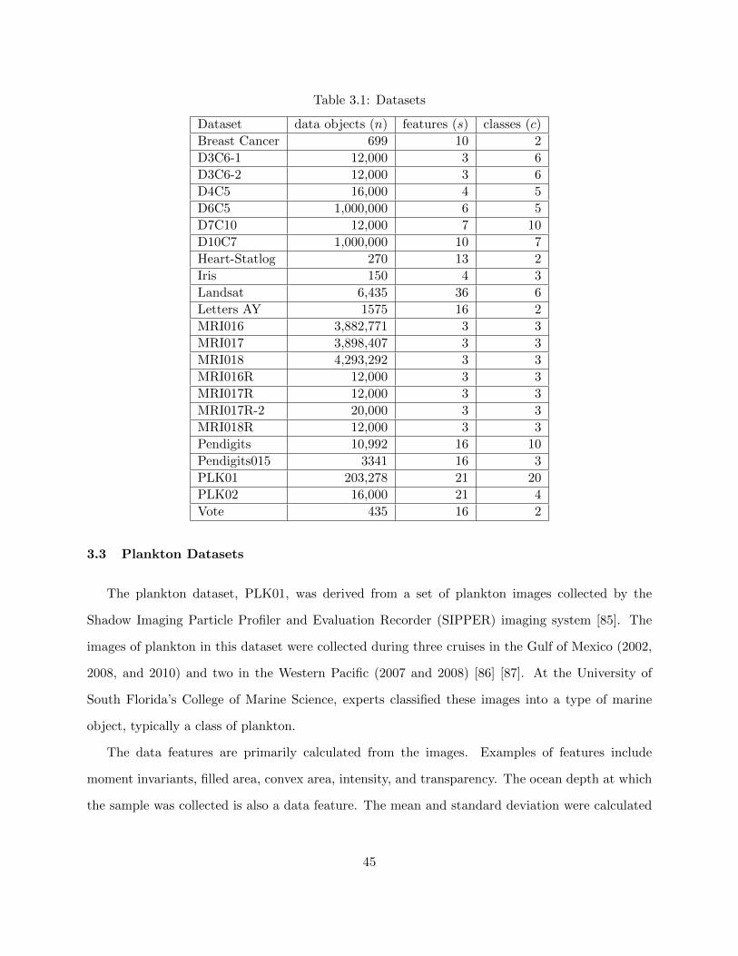
Table 3.1: Datasets
Dataset data objects (n) features (s) classes (c)
Breast Cancer 699 10 2
D3C6-1 12,000 3 6
D3C6-2 12,000 3 6
D4C5 16,000 4 5
D6C5 1,000,000 6 5
D7C10 12,000 7 10
D10C7 1,000,000 10 7
Heart-Statlog 270 13 2
Iris 150 4 3
Landsat 6,435 36 6
Letters AY 1575 16 2
MRI016 3,882,771 3 3
MRI017 3,898,407 3 3
MRI018 4,293,292 3 3
MRI016R 12,000 3 3
MRI017R 12,000 3 3
MRI017R-2 20,000 3 3
MRI018R 12,000 3 3
Pendigits 10,992 16 10
Pendigits015 3341 16 3
PLK01 203,278 21 20
PLK02 16,000 21 4
Vote 435 16 2
3.3 Plankton Datasets
The plankton dataset, PLK01, was derived from a set of plankton images collected by the
Shadow Imaging Particle Profiler and Evaluation Recorder (SIPPER) imaging system [85]. The
images of plankton in this dataset were collected during three cruises in the Gulf of Mexico (2002,
2008, and 2010) and two in the Western Pacific (2007 and 2008) [86] [87]. At the University of
South Florida’s College of Marine Science, experts classified these images into a type of marine
object, typically a class of plankton.
The data features are primarily calculated from the images. Examples of features include
moment invariants, filled area, convex area, intensity, and transparency. The ocean depth at which
the sample was collected is also a data feature. The mean and standard deviation were calculated
45
for each feature. The values for each feature were fitted to a standard normal distribution, so that
the mean feature value would equal zero and the feature value would equal the number of standard
deviations the value is above or below the mean [87].
Initially, there were a total of 482,719 data objects, with 88 features, representing 168 classes of
marine object. The number of data objects in the classes ranged from a single example (elongate
phytoplankton: chaetoceros) to 99,414 (noise: air bubble). Attempts cluster the entire dataset
with c = 168 did not provide stable results. The data objects belonging to noise, detritus, and
other small, non-homogeneous classes were removed, and the remaining data objects were placed
in random order. Using the WEKA data mining tool [88], feature selection was performed with
Consistency Subset Evaluation and Linear Forward Selection [89]. These efforts left 203,278 data
objects and 21 features. Analysis of the cleaned dataset showed 20 predominant classes.
A second dataset, PLK02, was created out of PLK01. A total of 16,000 data objects was
randomly selected from PLK01. Each selected data object was in one of four classes: crustacean
ostracod, elongate chaetognath, elongate strands, and protist. An equal number of data objects
(4,000) was selected from each class.
The full plankton dataset (PLK01) is very challenging to cluster using the FCM family of
algorithms. One of the reasons is its imbalanced data distribution by class [90]. The FCM algorithm
and other algorithms that reduce a squared error term perform best when the distribution by class
is roughly equal [91]. The PLK02 dataset, with an equal number of data objects in each class,
represents a lesser challenge.
3.4 UCI Datasets
The University of California, Irvine (UCI) Machine Learning Repository is a resource well-known
to data scientists [92]. As of 2013, it holds over 240 pre-processed datasets for experimentation
and testing of machine learning algorithms. Several datasets from this repository were used in
experiments.
46

3.4.1 Breast Cancer (Wisconsin)
The Wisconsin Breast Cancer dataset consists of test results for 699 clinical cases [93]. Each
of the 10 features is the value of a diagnostic measure, scaled between 1 and 10. The class values,
which were not used in the research, indicate if the test results indicated a malignant or benign
tumor.
3.4.2 Heart-Statlog
The Heart-Statlog dataset consists of information from 270 clinical cases [94]. Each of the 13
features is the value of a diagnostic measure. The class values, which were not used in the research,
indicate the presence or absence of heart disease.
3.4.3 Iris
The Iris dataset consists of field measurements of 150 iris flowers. Each of the four features are
the length or width of some part of the flower. The class values are the three different species of
iris measured [95].
3.4.4 Landsat
The Landsat dataset is imagery from the National Aeronautics and Space Administration’s
(NASA) Landsat Multispectral Scanner (MSS). Each of the 6,435 data objects is derived from a
3 × 3 pixel area of imagery of the Earth’s surface. The 36 features are the intensities of light in
four spectral bands for each of the nine pixels. The values are integers ranging from 0 to 255. The
dataset was clustered into six classes, corresponding to six different land cover types [96].
3.4.5 Letters
The Letters dataset consists of data from 20,000 images, each of which is one of the 26 capital
letters in the English language. Each image is unique; the original image was a letter in 1 of 20
fonts which was randomly distorted. The image data features are each converted to an integer
ranging from 0 to 15 [97].
47
A subset dataset was created from letters that just consists of the letters ’A’ and ’Y’. This
dataset consists of 1,575 data objects.
3.4.6 Pendigits
Pendigits is a collection of 10,992 handwritten numerals collected from 44 different writers. The
handwritten numerals were plotted on an x× y coordinate grid. The 16 features are 8 (x, y) coor-
dinates from the handwritten numeral. The coordinates were spatially resampled to be separated
by an equal arc-length. The values are integers ranging from 0 to 100. The dataset was clustered
into ten classes, corresponding to numerals from 0 to 9 [98].
A subset dataset of Pendigits was created using just the digits 0, 1 and 5. It was appropriately
named Pendigits015 and consists of 3,341 data objects.
3.4.7 Vote
The Vote dataset holds the 1984 United States Congressional voting records. Each record
contains the votes of 435 Congressmen for 16 important votes that year [99]. ’Yes’ votes were
converted to equal ’1’ and ’No’ votes converted to equal ’0’. The class values, which were not used
in the research, are the political party of each Congressman.
3.5 Artificial
A total of six artificial datasets were created for experiments. A simple program was written
to generate artificial datasets. The program input consists of the locations of c cluster centers in
Rs as well as the desired variance and number of data objects for each cluster center. Each data
object deviates from its cluster center in each dimension by a random amount determined by a
gaussian distribution using the provided variance. The generated examples were then output in
random order. Each artificial dataset was provided its own unique random seed, to ensure that the
dataset generation program did not produce the same series of pseudo-random numbers.
48
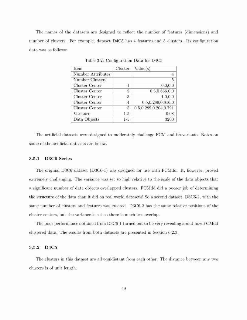
The names of the datasets are designed to reflect the number of features (dimensions) and
number of clusters. For example, dataset D4C5 has 4 features and 5 clusters. Its configuration
data was as follows:
Table 3.2: Configuration Data for D4C5
Item Cluster Value(s)
Number Attributes 4
Number Clusters 5
Cluster Center 1 0,0,0,0
Cluster Center 2 0.5,0.866,0,0
Cluster Center 3 1,0,0,0
Cluster Center 4 0.5,0.289,0.816,0
Cluster Center 5 0.5,0.289,0.204,0.791
Variance 1-5 0.08
Data Objects 1-5 3200
The artificial datasets were designed to moderately challenge FCM and its variants. Notes on
some of the artificial datasets are below.
3.5.1 D3C6 Series
The original D3C6 dataset (D3C6-1) was designed for use with FCMdd. It, however, proved
extremely challenging. The variance was set so high relative to the scale of the data objects that
a significant number of data objects overlapped clusters. FCMdd did a poorer job of determining
the structure of the data than it did on real world datasets! So a second dataset, D3C6-2, with the
same number of clusters and features was created. D3C6-2 has the same relative positions of the
cluster centers, but the variance is set so there is much less overlap.
The poor performance obtained from D3C6-1 turned out to be very revealing about how FCMdd
clustered data. The results from both datasets are presented in Section 6.2.3.
3.5.2 D4C5
The clusters in this dataset are all equidistant from each other. The distance between any two
clusters is of unit length.
49
Chapter 4: A Simple Experiment
“ You can observe a lot by watching.” - Lawrence “Yogi” Berra [2]
4.1 Introduction
FCM forms the basis for many accelerated algorithms [62] [64] [68] [100] [46] [65] [16]. Some of
these algorithms were discussed in Chapter 2. It is difficult to select the best accelerated algorithm
for a particular application, despite a careful review of the published literature. This is so because
the research in published works was performed on disparate hardware, operating systems, and code
bases. Speedup and quality metrics used in published works are not uniform.4
A series of experiments was conducted using FCM and four accelerated variants (SPFCM,
OFCM, eFFCM, rseFCM) [22]. Analysis of the results compared the speedup and quality of
the accelerated variants to FCM and to each other. The goals of the experimentation were to
gain insight into why different accelerated algorithms obtain different levels of performance and to
explore ways to improve this class of algorithm.
4.2 Experimental Procedures
Experiments were conducted using five datasets: MRI016, MRI017, MRI18, Pendigits, and
Landsat5. Details on the datasets are in Chapter 3. Details on the software implementation of the
algorithms are in Appendix A.2.
For each experiment runtime and quality metric values were recorded. As noted in Section
2.1.2, this class of algorithms produces non-deterministic results when random initialization is
4Some of the material in this chapter has been previously published by me [22] and is re-used under terms of thecopyright c© 2012 IEEE.
5Results for an initial set of experiments were published in [22]. The results presented here used an updatedcodebase that implemented Kolen’s optimization (Section A.2.3) and improved precision.
50
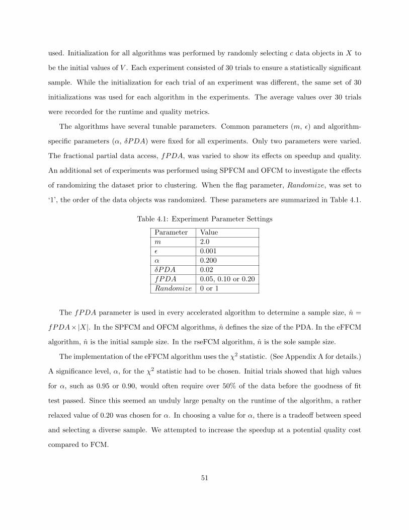
used. Initialization for all algorithms was performed by randomly selecting c data objects in X to
be the initial values of V . Each experiment consisted of 30 trials to ensure a statistically significant
sample. While the initialization for each trial of an experiment was different, the same set of 30
initializations was used for each algorithm in the experiments. The average values over 30 trials
were recorded for the runtime and quality metrics.
The algorithms have several tunable parameters. Common parameters (m, ε) and algorithm-
specific parameters (α, δPDA) were fixed for all experiments. Only two parameters were varied.
The fractional partial data access, fPDA, was varied to show its effects on speedup and quality.
An additional set of experiments was performed using SPFCM and OFCM to investigate the effects
of randomizing the dataset prior to clustering. When the flag parameter, Randomize, was set to
‘1’, the order of the data objects was randomized. These parameters are summarized in Table 4.1.
Table 4.1: Experiment Parameter Settings
Parameter Value
m 2.0
ε 0.001
α 0.200
δPDA 0.02
fPDA 0.05, 0.10 or 0.20
Randomize 0 or 1
The fPDA parameter is used in every accelerated algorithm to determine a sample size, n =
fPDA×|X|. In the SPFCM and OFCM algorithms, n defines the size of the PDA. In the eFFCM
algorithm, n is the initial sample size. In the rseFCM algorithm, n is the sole sample size.
The implementation of the eFFCM algorithm uses the χ2 statistic. (See Appendix A for details.)
A significance level, α, for the χ2 statistic had to be chosen. Initial trials showed that high values
for α, such as 0.95 or 0.90, would often require over 50% of the data before the goodness of fit
test passed. Since this seemed an unduly large penalty on the runtime of the algorithm, a rather
relaxed value of 0.20 was chosen for α. In choosing a value for α, there is a tradeoff between speed
and selecting a diverse sample. We attempted to increase the speedup at a potential quality cost
compared to FCM.
51

For each experiment the results from all algorithms on the same dataset with identical parameter
settings were recorded. Regarding each algorithm, runtime, the number of iterations to termination,
the cluster center positions, and Rm were recorded.
4.3 Results
The metrics collected were used to calculate relative speedup (SU), DQRm%, DFV%, and
CC% between the five algorithms for the five datasets. This created a large volume of data; Table
4.2 shows results for just one dataset (MRI016), one fPDA (0.05), and one metric (SU).
Table 4.3 shows, with respect to FCM, each algorithm’s speedup and quality for each PDA,
over all the MRI datasets. The average of results for the MRI datasets are reported, because there
was little difference between them. The Pendigits and Landsat datasets (Tables 4.4 and 4.5) had
more differences between them.
The speedups of each accelerated algorithm vs. FCM ranged from below 1 to over 10. The
quality and fidelity metrics of each accelerated algorithm deviated from FCM by 0% to 11%.
Table 4.2: Speedup Comparison for MRI016, fPDA = 0.05
Algorithm vs. FCM vs. SPFCM vs. OFCM vs. eFFCM vs. rseFCM
FCM 1.0000 0.2479 0.6161 0.4966 0.1434
SPFCM 4.0343 1.0000 2.4854 2.0034 0.5786
OFCM 1.6232 0.4024 1.0000 0.8061 0.2328
eFFCM 2.0137 0.4992 1.2406 1.0000 0.2888
rseFCM 6.9721 1.7282 4.2953 3.4623 1.0000
4.4 Discussion
The results show real differences in the speedup and quality of FCM’s accelerated variants.
The quality measures of all accelerated variants represent a degradation from FCM. On the
MRI datasets, for all fPDAs and quality metrics, there is only a little deviation from the reference
algorithm, FCM (Table 4.3). Compared to the other datasets, the MRI datasets have a larger
number of data objects (> 3× 10⁷), and lower numbers of data features (3) and clusters (3).
52
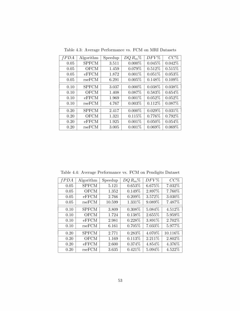
Table 4.3: Average Performance vs. FCM on MRI Datasets
fPDA Algorithm Speedup DQRm% DFV% CC%
0.05 SPFCM 3.511 0.000% 0.045% 0.042%
0.05 OFCM 1.459 0.079% 0.512% 0.515%
0.05 eFFCM 1.872 0.001% 0.051% 0.053%
0.05 rseFCM 6.291 0.005% 0.148% 0.109%
0.10 SPFCM 3.037 0.000% 0.038% 0.038%
0.10 OFCM 1.408 0.087% 0.583% 0.654%
0.10 eFFCM 1.969 0.001% 0.052% 0.052%
0.10 rseFCM 4.767 0.003% 0.112% 0.087%
0.20 SPFCM 2.417 0.000% 0.029% 0.031%
0.20 OFCM 1.321 0.115% 0.776% 0.792%
0.20 eFFCM 1.925 0.001% 0.050% 0.054%
0.20 rseFCM 3.005 0.001% 0.069% 0.069%
Table 4.4: Average Performance vs. FCM on Pendigits Dataset
fPDA Algorithm Speedup DQRm% DFV% CC%
0.05 SPFCM 5.121 0.653% 6.675% 7.032%
0.05 OFCM 1.352 0.149% 2.897% 7.760%
0.05 eFFCM 2.766 0.209% 3.572% 3.030%
0.05 rseFCM 10.599 1.331% 9.089% 7.487%
0.10 SPFCM 3.809 0.308% 5.084% 4.512%
0.10 OFCM 1.724 0.138% 2.655% 5.959%
0.10 eFFCM 2.981 0.228% 3.891% 2.702%
0.10 rseFCM 6.161 0.705% 7.033% 5.977%
0.20 SPFCM 2.771 0.283% 4.070% 10.116%
0.20 OFCM 1.169 0.113% 2.211% 2.802%
0.20 eFFCM 2.600 0.374% 4.854% 4.376%
0.20 rseFCM 3.635 0.421% 5.094% 4.522%
53

Table 4.5: Average Performance vs. FCM on Landsat Dataset
fPDA Algorithm Speedup DQRm% DFV% CC%
0.05 SPFCM 1.914 0.469% 1.310% 1.321%
0.05 OFCM 1.045 0.635% 1.200% 5.206%
0.05 eFFCM 1.309 0.163% 0.550% 0.389%
0.05 rseFCM 3.353 2.009% 2.241% 1.601%
0.10 SPFCM 1.703 0.513% 1.025% 1.134%
0.10 OFCM 1.030 0.918% 2.201% 10.956%
0.10 eFFCM 1.320 0.190% 0.594% 0.280%
0.10 rseFCM 2.745 0.779% 1.314% 0.653%
0.20 SPFCM 1.534 0.097% 0.505% 0.326%
0.20 OFCM 0.907 0.777% 1.740% 9.029%
0.20 eFFCM 1.315 0.205% 0.611% 0.202%
0.20 rseFCM 2.151 0.337% 0.831% 0.357%
The Pendigits and Landsat results show that DQRm% deviates from FCM by 0.1% to 2.0%
(Tables 4.4 and 4.5). On average, this is a much higher deviation than in the MRI datasets. The
DFV% and CC% metrics from the Pendigits and Landsat results are, on average, much higher
than corresponding values in the MRI datasets. Occasionally, corresponding values are two orders
of magnitude higher! The Pendigits and Landsat datasets both have fewer objects and a greater
number of features than the MRI datasets.
Overall, the gains in speed are modest; the greatest speedup is around 10 times. In general,
speedup was inversely proportional to the total sample size (eFFCM and rseFCM) or the fPDA
(SPFCM and OFCM). Analyses of the speedup and effects on quality for each accelerated variant
are given in the subsections below.
4.4.1 rseFCM’s Speedup
This accelerated variant of FCM reduces runtime by reducing the size of the dataset. The FCM
runtime complexity is linear with respect to n, so a reduction in n would have a corresponding
reduction in runtime. The rseFCM algorithm should therefore have a speedup inversely proportional
to fPDA, but this does not take into account the time needed for random selection of data from
54
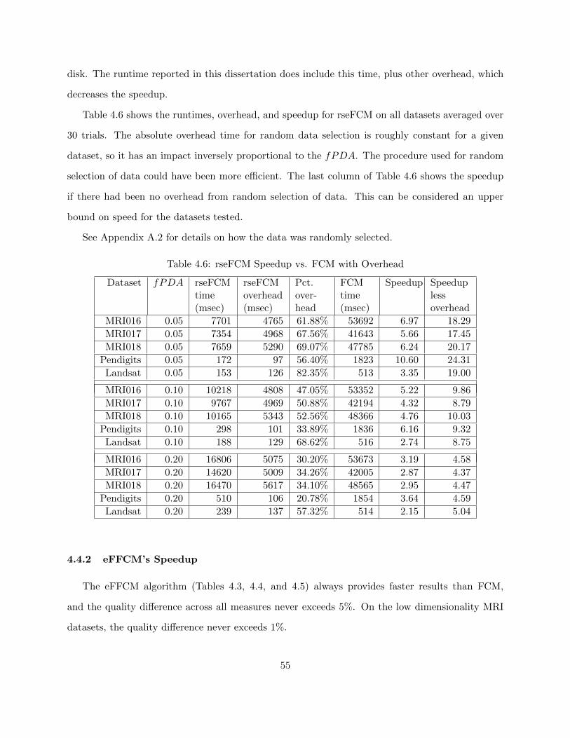
disk. The runtime reported in this dissertation does include this time, plus other overhead, which
decreases the speedup.
Table 4.6 shows the runtimes, overhead, and speedup for rseFCM on all datasets averaged over
30 trials. The absolute overhead time for random data selection is roughly constant for a given
dataset, so it has an impact inversely proportional to the fPDA. The procedure used for random
selection of data could have been more efficient. The last column of Table 4.6 shows the speedup
if there had been no overhead from random selection of data. This can be considered an upper
bound on speed for the datasets tested.
See Appendix A.2 for details on how the data was randomly selected.
Table 4.6: rseFCM Speedup vs. FCM with Overhead
Dataset fPDA rseFCMtime(msec)
rseFCMoverhead(msec)
Pct.over-head
FCMtime(msec)
Speedup Speeduplessoverhead
MRI016 0.05 7701 4765 61.88% 53692 6.97 18.29
MRI017 0.05 7354 4968 67.56% 41643 5.66 17.45
MRI018 0.05 7659 5290 69.07% 47785 6.24 20.17
Pendigits 0.05 172 97 56.40% 1823 10.60 24.31
Landsat 0.05 153 126 82.35% 513 3.35 19.00
MRI016 0.10 10218 4808 47.05% 53352 5.22 9.86
MRI017 0.10 9767 4969 50.88% 42194 4.32 8.79
MRI018 0.10 10165 5343 52.56% 48366 4.76 10.03
Pendigits 0.10 298 101 33.89% 1836 6.16 9.32
Landsat 0.10 188 129 68.62% 516 2.74 8.75
MRI016 0.20 16806 5075 30.20% 53673 3.19 4.58
MRI017 0.20 14620 5009 34.26% 42005 2.87 4.37
MRI018 0.20 16470 5617 34.10% 48565 2.95 4.47
Pendigits 0.20 510 106 20.78% 1854 3.64 4.59
Landsat 0.20 239 137 57.32% 514 2.15 5.04
4.4.2 eFFCM’s Speedup
The eFFCM algorithm (Tables 4.3, 4.4, and 4.5) always provides faster results than FCM,
and the quality difference across all measures never exceeds 5%. On the low dimensionality MRI
datasets, the quality difference never exceeds 1%.
55
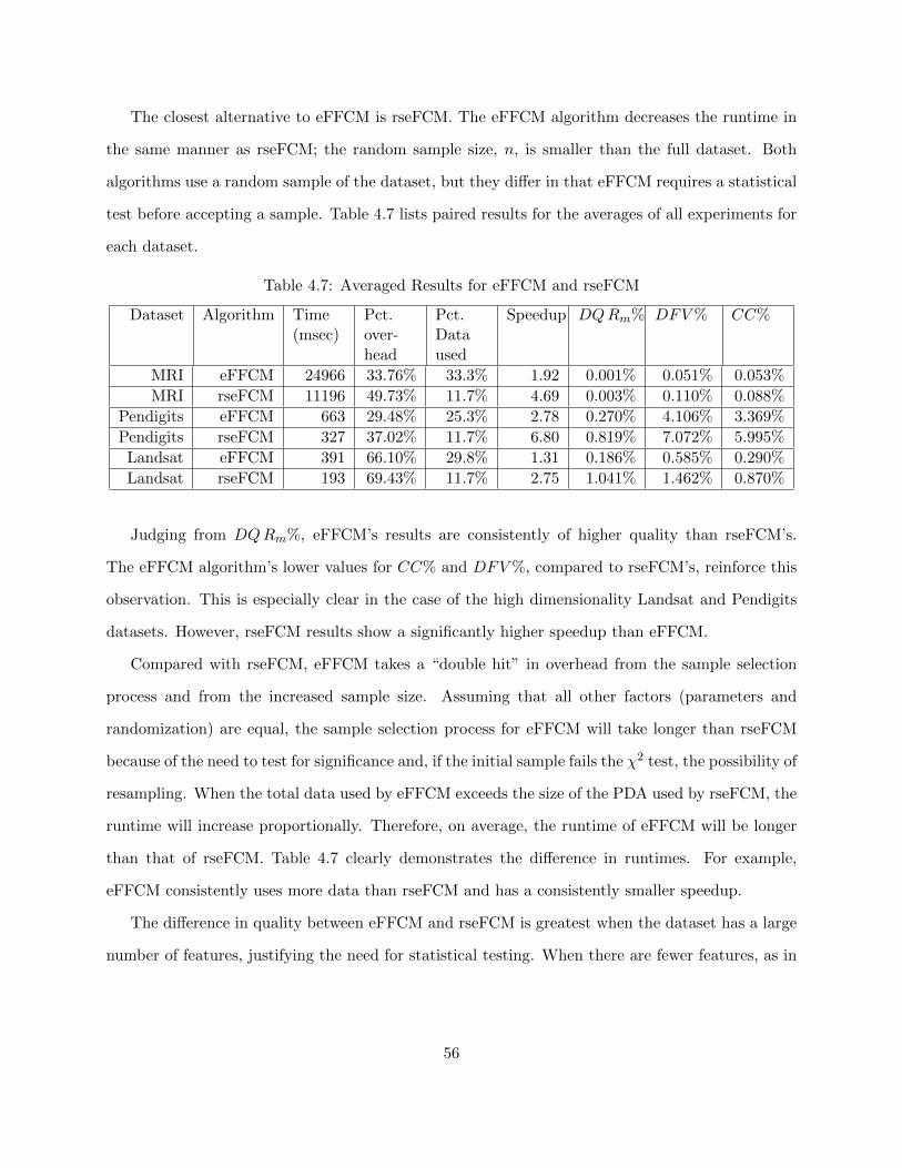
The closest alternative to eFFCM is rseFCM. The eFFCM algorithm decreases the runtime in
the same manner as rseFCM; the random sample size, n, is smaller than the full dataset. Both
algorithms use a random sample of the dataset, but they differ in that eFFCM requires a statistical
test before accepting a sample. Table 4.7 lists paired results for the averages of all experiments for
each dataset.
Table 4.7: Averaged Results for eFFCM and rseFCM
Dataset Algorithm Time(msec)
Pct.over-head
Pct.Dataused
Speedup DQRm% DFV% CC%
MRI eFFCM 24966 33.76% 33.3% 1.92 0.001% 0.051% 0.053%
MRI rseFCM 11196 49.73% 11.7% 4.69 0.003% 0.110% 0.088%
Pendigits eFFCM 663 29.48% 25.3% 2.78 0.270% 4.106% 3.369%
Pendigits rseFCM 327 37.02% 11.7% 6.80 0.819% 7.072% 5.995%
Landsat eFFCM 391 66.10% 29.8% 1.31 0.186% 0.585% 0.290%
Landsat rseFCM 193 69.43% 11.7% 2.75 1.041% 1.462% 0.870%
Judging from DQRm%, eFFCM’s results are consistently of higher quality than rseFCM’s.
The eFFCM algorithm’s lower values for CC% and DFV%, compared to rseFCM’s, reinforce this
observation. This is especially clear in the case of the high dimensionality Landsat and Pendigits
datasets. However, rseFCM results show a significantly higher speedup than eFFCM.
Compared with rseFCM, eFFCM takes a “double hit” in overhead from the sample selection
process and from the increased sample size. Assuming that all other factors (parameters and
randomization) are equal, the sample selection process for eFFCM will take longer than rseFCM
because of the need to test for significance and, if the initial sample fails the χ2 test, the possibility of
resampling. When the total data used by eFFCM exceeds the size of the PDA used by rseFCM, the
runtime will increase proportionally. Therefore, on average, the runtime of eFFCM will be longer
than that of rseFCM. Table 4.7 clearly demonstrates the difference in runtimes. For example,
eFFCM consistently uses more data than rseFCM and has a consistently smaller speedup.
The difference in quality between eFFCM and rseFCM is greatest when the dataset has a large
number of features, justifying the need for statistical testing. When there are fewer features, as in
56

the case of the MRI datasets, rseFCM has quality nearly equal to eFFCM’s, but it has a greater
speedup.
4.4.3 SPFCM’s Speedup
The SPFCM algorithm provides a reliable speedup with little or no loss in quality over all
datasets. The SPFCM results are shown in Table 4.8.
The speedup ranges from roughly 1.5 to 5.1, but this takes into account the time needed to
place the data in random order, disk I/O, and other overhead. In some applications, the data is
naturally in random order or has been pre-randomized. If the speedup calculation is adjusted to
make this assumption, the speedup ranges from 3.2 to 8.8. The percentage of the runtime taken
by overhead from randomization of the dataset is listed in the column labeled ‘Pct. overhead’ in
Table 4.8. The difference in speedup is shown in the columns ‘Speedup’ and ‘Adj. Speedup’.
The speedup was inversely proportional with respect to the fPDA across all datasets. This
was predicted from the analysis of the runtime complexity. SPFCM’s runtime is linear with respect
to the number of data objects in each PDA. The speedup occurred because the weighted cluster
centers passed to the next PDA were a better estimate of the final cluster centers compared with
random initialization. Thus, fewer iterations were required until termination. When fPDA was
large, there were fewer PDAs and fewer opportunities to reduce the number of iterations. Details
on the runtime complexity are in Section 2.3.2.1.
Based on DQRm%, the FCM and SPFCM provide the same quality on the MRI datasets.
The corresponding cluster change percentages are very low, ranging from 0.010% to 0.067%. The
Landsat and Pendigits datasets have small degradations in Rm of less than 1%. Their cluster
change percentages, however, are much higher than those of the MRI datasets, ranging from 0.3%
to 10.1%.
The poorer fidelity, as measured by CC%, in these datasets is not surprising. They both have
more attributes and clusters than the MRI datasets, and therefore more boundary areas between
clusters in higher-dimensional space. So a small perturbation in cluster center position has the
57
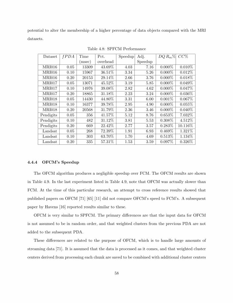
potential to alter the membership of a higher percentage of data objects compared with the MRI
datasets.
Table 4.8: SPFCM Performance
Dataset fPDA Time(msec)
Pct.overhead
Speedup Adj.Speedup
DQRm% CC%
MRI016 0.05 13309 43.69% 4.03 7.16 0.000% 0.010%
MRI016 0.10 15967 36.51% 3.34 5.26 0.000% 0.012%
MRI016 0.20 20153 29.14% 2.66 3.76 0.000% 0.018%
MRI017 0.05 13071 45.52% 3.19 5.85 0.000% 0.049%
MRI017 0.10 14976 39.08% 2.82 4.62 0.000% 0.047%
MRI017 0.20 18865 31.18% 2.23 3.24 0.000% 0.036%
MRI018 0.05 14430 44.80% 3.31 6.00 0.001% 0.067%
MRI018 0.10 16377 39.78% 2.95 4.90 0.000% 0.055%
MRI018 0.20 20568 31.79% 2.36 3.46 0.000% 0.040%
Pendigits 0.05 356 41.57% 5.12 8.76 0.653% 7.032%
Pendigits 0.10 482 31.12% 3.81 5.53 0.308% 4.512%
Pendigits 0.20 669 22.42% 2.77 3.57 0.283% 10.116%
Landsat 0.05 268 72.39% 1.91 6.93 0.469% 1.321%
Landsat 0.10 303 63.70% 1.70 4.69 0.513% 1.134%
Landsat 0.20 335 57.31% 1.53 3.59 0.097% 0.326%
4.4.4 OFCM’s Speedup
The OFCM algorithm produces a negligible speedup over FCM. The OFCM results are shown
in Table 4.9. In the last experiment listed in Table 4.9, note that OFCM was actually slower than
FCM. At the time of this particular research, an attempt to cross reference results showed that
published papers on OFCM [71] [65] [11] did not compare OFCM’s speed to FCM’s. A subsequent
paper by Havens [16] reported results similar to these.
OFCM is very similar to SPFCM. The primary differences are that the input data for OFCM
is not assumed to be in random order, and that weighted clusters from the previous PDA are not
added to the subsequent PDA.
These differences are related to the purpose of OFCM, which is to handle large amounts of
streaming data [71]. It is assumed that the data is processed as it comes, and that weighted cluster
centers derived from processing each chunk are saved to be combined with additional cluster centers
58
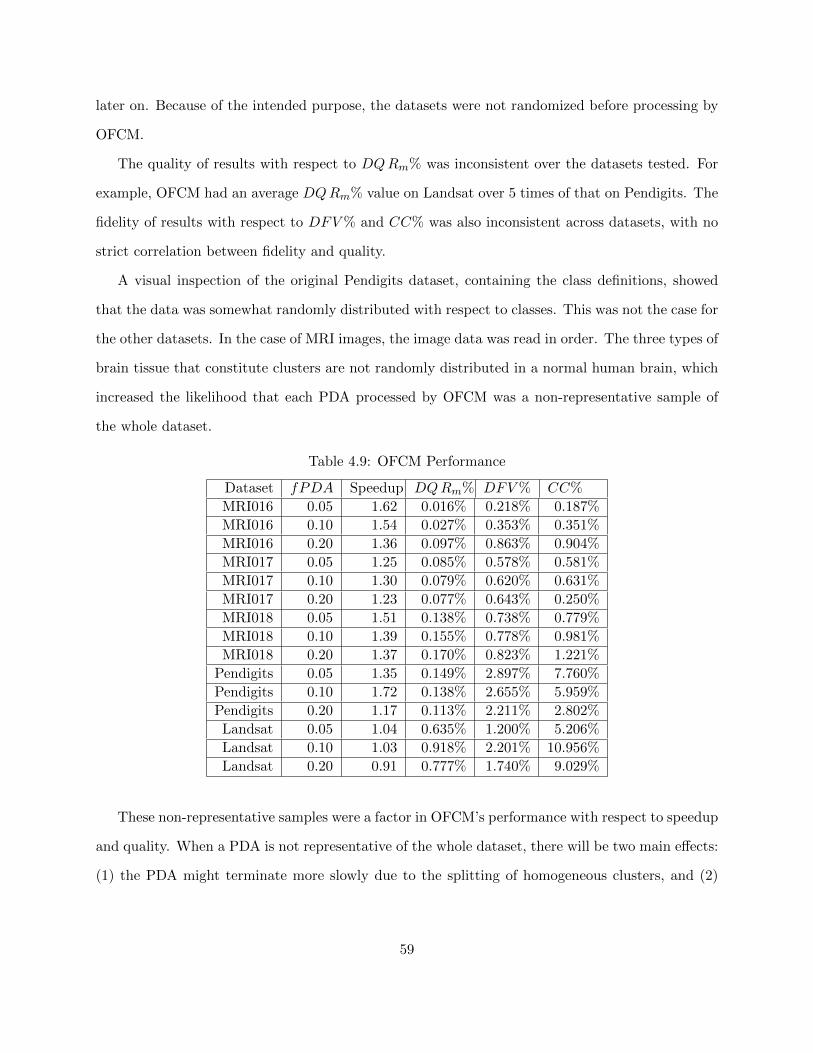
later on. Because of the intended purpose, the datasets were not randomized before processing by
OFCM.
The quality of results with respect to DQRm% was inconsistent over the datasets tested. For
example, OFCM had an average DQRm% value on Landsat over 5 times of that on Pendigits. The
fidelity of results with respect to DFV% and CC% was also inconsistent across datasets, with no
strict correlation between fidelity and quality.
A visual inspection of the original Pendigits dataset, containing the class definitions, showed
that the data was somewhat randomly distributed with respect to classes. This was not the case for
the other datasets. In the case of MRI images, the image data was read in order. The three types of
brain tissue that constitute clusters are not randomly distributed in a normal human brain, which
increased the likelihood that each PDA processed by OFCM was a non-representative sample of
the whole dataset.
Table 4.9: OFCM Performance
Dataset fPDA Speedup DQRm% DFV% CC%
MRI016 0.05 1.62 0.016% 0.218% 0.187%
MRI016 0.10 1.54 0.027% 0.353% 0.351%
MRI016 0.20 1.36 0.097% 0.863% 0.904%
MRI017 0.05 1.25 0.085% 0.578% 0.581%
MRI017 0.10 1.30 0.079% 0.620% 0.631%
MRI017 0.20 1.23 0.077% 0.643% 0.250%
MRI018 0.05 1.51 0.138% 0.738% 0.779%
MRI018 0.10 1.39 0.155% 0.778% 0.981%
MRI018 0.20 1.37 0.170% 0.823% 1.221%
Pendigits 0.05 1.35 0.149% 2.897% 7.760%
Pendigits 0.10 1.72 0.138% 2.655% 5.959%
Pendigits 0.20 1.17 0.113% 2.211% 2.802%
Landsat 0.05 1.04 0.635% 1.200% 5.206%
Landsat 0.10 1.03 0.918% 2.201% 10.956%
Landsat 0.20 0.91 0.777% 1.740% 9.029%
These non-representative samples were a factor in OFCM’s performance with respect to speedup
and quality. When a PDA is not representative of the whole dataset, there will be two main effects:
(1) the PDA might terminate more slowly due to the splitting of homogeneous clusters, and (2)
59
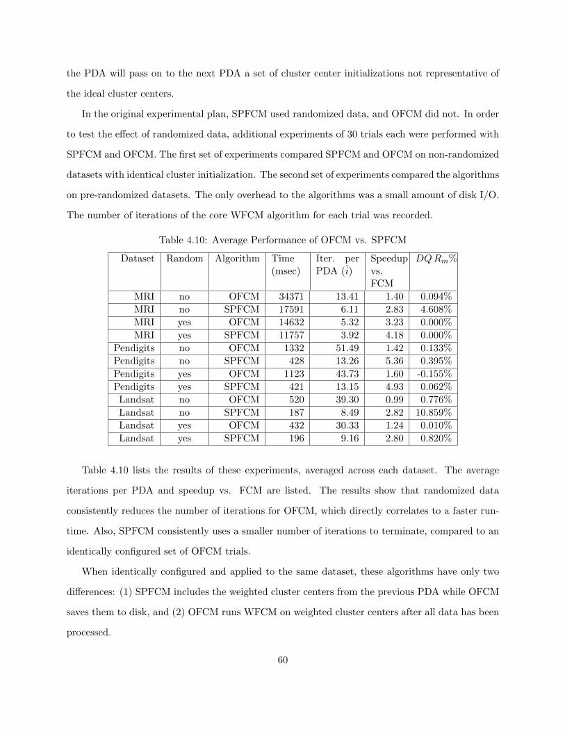
the PDA will pass on to the next PDA a set of cluster center initializations not representative of
the ideal cluster centers.
In the original experimental plan, SPFCM used randomized data, and OFCM did not. In order
to test the effect of randomized data, additional experiments of 30 trials each were performed with
SPFCM and OFCM. The first set of experiments compared SPFCM and OFCM on non-randomized
datasets with identical cluster initialization. The second set of experiments compared the algorithms
on pre-randomized datasets. The only overhead to the algorithms was a small amount of disk I/O.
The number of iterations of the core WFCM algorithm for each trial was recorded.
Table 4.10: Average Performance of OFCM vs. SPFCM
Dataset Random Algorithm Time(msec)
Iter. perPDA (i)
Speedupvs.FCM
DQRm%
MRI no OFCM 34371 13.41 1.40 0.094%
MRI no SPFCM 17591 6.11 2.83 4.608%
MRI yes OFCM 14632 5.32 3.23 0.000%
MRI yes SPFCM 11757 3.92 4.18 0.000%
Pendigits no OFCM 1332 51.49 1.42 0.133%
Pendigits no SPFCM 428 13.26 5.36 0.395%
Pendigits yes OFCM 1123 43.73 1.60 -0.155%
Pendigits yes SPFCM 421 13.15 4.93 0.062%
Landsat no OFCM 520 39.30 0.99 0.776%
Landsat no SPFCM 187 8.49 2.82 10.859%
Landsat yes OFCM 432 30.33 1.24 0.010%
Landsat yes SPFCM 196 9.16 2.80 0.820%
Table 4.10 lists the results of these experiments, averaged across each dataset. The average
iterations per PDA and speedup vs. FCM are listed. The results show that randomized data
consistently reduces the number of iterations for OFCM, which directly correlates to a faster run-
time. Also, SPFCM consistently uses a smaller number of iterations to terminate, compared to an
identically configured set of OFCM trials.
When identically configured and applied to the same dataset, these algorithms have only two
differences: (1) SPFCM includes the weighted cluster centers from the previous PDA while OFCM
saves them to disk, and (2) OFCM runs WFCM on weighted cluster centers after all data has been
processed.
60
Let us first consider difference (2). An examination of the trial diagnostic logs showed that the
final step of OFCM (in which the weighted data objects are clustered) only added between 2 and
7 iterations. For the datasets used in experiments, the number of weighted data objects clustered
in this step is only between 15 and 200. This final step of OFCM adds only a negligible amount of
time.
This leaves difference (1). OFCM uses the positions of the previous c cluster centers as initial
values for V , but SPFCM uses both the positions for V and the c weighted data objects. Examina-
tion of Equation (2.15) shows how the weights associated with the data objects influence the values
in V . OFCM’s PDAs lack both the data objects and their weights, so it takes longer to terminate
with the initialized values. This was verified by reviewing the experiments’ diagnostic logs. Despite
identical initialization, OFCM required more iterations to terminate per PDA. In the course of the
investigation, it was also discovered that the number of iterations required for SPFCM to terminate
dropped to a very low level, very quickly. We note that the weights increase for each new PDA.
This has significant implications that are discussed in Section 5.3.
Table 4.10 also lists the DQRm% for each experiment. For all experiments, OFCM has a
lower value for DQRm% than SPFCM does under identical conditions.6 Earlier remarks on the
experimental results state that OFCM has quality inferior to SPFCM’s on the MRI and Landsat
datasets, but these remarks compared OFCM clustering non-randomized datasets.
SPFCM’s speedup is superior to OFCM’s for the same reasons that its quality is inferior.
SPFCM passes weighted cluster centers to each subsequent PDA to be processed by WFCM. After
the first few PDAs, these weighted cluster centers tend to dominate. Consider when fPDA = 0.05.
After 10 PDAs are clustered, the weighted cluster centers represent over 50% of the dataset! A
review of the diagnostic logs verified that the cluster center positions did not deviate much after
the first few PDAs had been clustered. So, if the initial PDAs are not proportional to the whole
dataset, the final set of cluster centers may be influenced negatively by the initial PDAs weighted
cluster centers.
6On the MRI datasets, OFCM has a slightly lower DQRm% than SPFCM, but Table 4.10 does not have theprecision to show it.
61
In contrast, OFCM does not cluster the combined dataset of weighted cluster centers until the
final step. The results from each PDA have equal influence on the final partition produced.
4.5 Conclusions
4.5.1 Assessing Quality
While the algorithms are designed to reduce Rm, their underlying purpose is to partition the
dataset. Changes to the partition are recorded in the CC% metric. In Tables 4.4 and 4.5, very
small values of DQRm% correlate to large changes in cluster assignments (CC%). Consequently,
only using the objective function value to determine how close two partitions are can be deceiving.
To assess fidelity properly when comparing accelerated algorithms, both a metric to assess the
functioning of the algorithm, such as DQRm%, and a metric to assess its effects, such as CC%,
are needed.
The original premise of the experiment was that the FCM algorithm would serve as a reference
for performance for the other algorithms. In Table 4.10, the comparison between SPFCM and
OFCM, note that one of the DQRm% entries for Pendigits is negative.
The DQRm% metric was calculated using Equation 2.20, substituting the Rm value for FCM
as Rm2. Negative values for the DQRm% indicate that the candidate algorithm had, on average,
a lower Rm value than FCM. In this case, one could say the quality of OFCM is better because the
objective function value being minimized is lower.
Table 4.10 lists averages over experiments. For the pre-randomized Pendigits dataset clustered
by OFCM, the DQRm% values for all experiments were negative. A one-tailed Welch’s t-test
(Section 2.4.7.1) was employed in order to ascertain whether the difference between FCM and
OFCM for the experiment with fPDA = 0.10 was significant. The DQRm% is only −0.1974%,
but the t-test yielded t = 1.83 with 29 d.f. This results in p = 0.0388, which may be considered
statistically significant at α = 0.05.
Originally, it was assumed that the DFV% and CC% fidelity metrics could express the objective
function quality loss of the accelerated variant as compared to the optimal reference algorithm,
FCM. This assumption was not valid when the accelerated variant had a lower Rm than FCM,
62
because the Rm value might have been a more desirable extremum. When DQRm% is negative,
the DFV% and CC% metrics express the quality improvement. Thus, it can be deceiving to only
view a partition-based fidelity metric, such as CC%, DFV%, or ARI in discussing quality.
The DFV% and CC% values listed in Tables 4.3, 4.4, and 4.5 showed some variation, but were
almost always the same order of magnitude for the same experiment. Deviation between the two
measures occurred when the fidelity, as measured by both metrics, was poor. This makes sense
because the DFV% assesses the change in cluster positions and CC% assesses the effects of that
change. This fact and the experimental results suggest that the DFV% and CC% metrics are
largely redundant. As the CC% metric reflects changes in the actual partition of the dataset, it is
a more meaningful metric.
4.5.2 Ranking the Algorithms
The FCM algorithm and four accelerated variants were compared with respect to speed and three
quality metrics. The code base and experiments were carefully constructed to ensure comparisons
on as equal a basis as possible.
The algorithms listed in order of speed from slowest to fastest are: FCM, OFCM, eFFCM,
SPFCM, and rseFCM. OFCM had a surprisingly small speed improvement over FCM. Analysis
showed that, despite improved starting cluster centers, each PDA took many iterations to terminate.
The differences between SPFCM and OFCM that influenced speed were data randomization and
the use of weighted data objects for cluster initialization.
The time taken to randomize data was included in the runtime calculations for eFFCM, SPFCM,
and rseFCM. This amount of time was often a significant percentage of the total runtime. If it
could be assumed that the data had been provided in random order, the speedups of these three
variants would improve further.
The algorithms are more difficult to rank in order of quality, because you want to consider fidelity
also. Judging solely from DQRm%, the eFFCM algorithm appears to have the best quality overall
and rseFCM the worst. There was little consistency, however, in quality measures across datasets.
Any ranking of “best algorithm” overall would be quite subjective. This study demonstrates that
63
tradeoffs must be made between speed and quality, and that there is variation in performance across
datasets.
4.5.3 Observations
The goals of the experimentation were to discover why accelerated clustering algorithms perform
like they do and how this knowledge can be leveraged to improve these algorithms.
Some accelerated algorithms produce a speedup by clustering only a sample of the dataset.
The rseFCM algorithm clusters a random sample of user-defined size. The eFFCM algorithm
also clusters a randomly selected sample, but it validates the sample with a statistical test. The
validation step increases the runtime, but it ensures a sample representative of the whole dataset.
The eFFCM algorithm, because of this sampling method, yielded higher-quality results compared
to those of rseFCM. These higher-quality results, however, came at the expense of speedup.
On the MRI datasets, rseFCM and eFFCM differed little in quality. This suggests that the
samples which rseFCM used were fairly representative of the whole dataset, and that little advan-
tage was gained by using a statistical test. The MRI datasets are large relative to the Pendigits
and Landsat datasets, and have a smaller number of clusters and data features. Recall that the
experimental setup used fPDA to determine the sample size. When the fPDA = 0.05, rseFCM
had a sample size 1/20 of the whole dataset: 194,139 from MRI016, but only 322 from Landsat.
The SPFCM and OFCM algorithms produce a speedup by incrementally clustering all the data,
one sample at a time. Representative objects hold the partition information from each sample.
Comparing SPFCM and OFCM, the experiments that used pre-randomized data were faster and
had better quality than those that did not. Again, the pre-randomized data is more likely to be
representative of the dataset as a whole. This has the apparent effect of improving speedup as well
as quality.
SPFCM was always faster than OFCM, regardless of whether or not the data had been pre-
randomized. For initialization, SPFCM used weighted data objects as cluster centers, unlike OFCM,
which used the cluster center positions. The existence of the weighted data objects influenced the
positions of the cluster centers, which resulted in fewer iterations. In Section 2.3.2.1, the runtime
64
complexity of SPFCM is shown to be identical to that of FCM. SPFCM’s speedup is due to
improved cluster center initialization after the initial PDA. The implementation of OFCM uses the
same strategy as SPFCM to initialize cluster centers. On identical datasets, the difference in speed
between SPFCM and OFCM is solely due to weighted cluster center initialization.
Regarding quality, the use of weighted cluster centers had the opposite effect. These weighted
data objects greatly influenced the cluster centers produced by each PDA. If the initial PDAs
clustered by SPFCM were not representative of the whole dataset, the final set of cluster centers
drifted to resemble the results of the initial PDAs. OFCM, however, clustered the best represen-
tatives of each PDA, which reflected the whole dataset better. Under identical conditions (dataset
randomization, algorithmic parameters), OFCM had consistently better quality than SPFCM. A
one-tailed Welch’s t-test (Section 2.4.7.1) was employed in order to ascertain whether the differences
in DQRm% between SPFCM and OFCM were significant. Over all 30 experiments conducted, the
least significant test yielded t = 1.99 with 29 d.f. This results in p = 0.0280, which may be consid-
ered statistically significant at α = 0.05. Thus one can conclude that OFCM provided statistically
significantly better quality results than SPFCM for the quality metric and α value used.
To sum up, SPFCM and rseFCM worked best on datasets with small numbers of features and
classes. The eFFCM algorithm had the best quality and fidelity on datasets with larger numbers
of features and classes, but the speedup was modest. The OFCM algorithm had the best quality
and fidelity on datasets with data objects that were already in random order with respect to class,
though the speedup was small. For every dataset, choice of algorithm represented a tradeoff of
speed and quality/fidelity.
Significant observations on the entire experiment are as follows:
• A smaller sample size decreases the runtime.
• A sample representative of the whole dataset results in a higher-quality partition.
• A larger sample size can make a statistical test superfluous.
• A distributed clustering solution, using representative objects, can produce high-quality re-
sults.
65

• An initial set of cluster centers closer to the final partition reduces runtime.
• SPFCM’s final reported set of cluster centers did not deviate significantly after the first few
PDAs were clustered.
• The use of weighted cluster centers for initialization reduces runtime.
• The use of weighted cluster centers can have a negative impact on quality if the sample is not
representative of the whole dataset.
These observations were condensed to the following ideas stated in Section 1.3
1. Use of a statistically significant sample of the dataset reduces runtime while preserving quality.
2. An algorithm designed to cluster the data incrementally can produce a high-quality result
when stopped before all data has been processed. This is especially true when the data is
presented in random order.
3. The use of representative objects, either weighted or un-weighted, can overcome difficulties
of scale, if properly utilized.
4. For a particular class of clustering algorithms, providing a “starting point” close to the optimal
solution reduces runtime and can improve quality.
In the following sections, these ideas will be explored further to create new accelerated clustering
algorithms.
66
Chapter 5: Accelerating FCM
“When you come to a fork in the road, take it.” - Lawrence “Yogi” Berra [2]
The experiments in Chapter 4 investigated the ways that FCM can be accelerated by reducing
n (eFFCM and rseFCM) or i (SPFCM and OFCM). The methods developed in this chapter seek
to accelerate FCM by simultaneously reducing n and i.7
5.1 Estimating the Random Sample Size
The accelerated clustering algorithms discussed in Section 2.3.1 and Chapter 4 sample the
dataset, but they typically do not use a statistical method to determine the sample size. Domingos
and Hulten’s technique [67] estimates the initial sample size using Hoeffding bounds for HCM
clustering, but this does not directly generalize to FCM [72].
The SPFCM algorithm uses a parameter (fPDA) to define a static sample size [46]. The
eFFCM algorithm uses a statistical test to validate a sample, but not to determine the sample size
[68] [72]. The mrFCM algorithm and Altman’s method also use a parameter to define the sample
size for cluster center initialization [62] [63]. The size of the sample influences the performance of
the algorithms [22], but the parameters in each case are determined empirically.
As suggested in [61], the sample must proportionally represent each cluster in order to provide
an improved starting point for an algorithm such as FCM, that uses alternating optimization. A
known difficulty in using a sample to generate starting points for a clustering algorithm occurs
when the sample fails to represent all clusters sufficiently [61] [62]. This results in skewed starting
7Content in this chapter is an edited version of the author’s previously published works [22] [23] and is re-usedunder terms of the copyright c© 2012 and 2013 IEEE. New material and analysis has been added.
67
points. One solution to this problem is to ensure that the sample has proportional representation.
This solution was suggested in [62] but not elaborated upon.
Gu (et al.) studied the effects of an improper starting sample size when using progressive
sampling on supervised learning problems [101]. They implemented a divergence test on a sample
to ensure it represented the dataset distribution. Similarly, in [68] and [73], Pal, Bezdek, and
Hathaway test the sample for the proportionality to the dataset as a whole, but they use the
sample for calculating the clustering solution rather than for estimating clusters for initialization.
Regardless, to ensure proportionality, this sort of technique requires collection of information from
the entire dataset. A larger sample of the dataset can be used for this purpose, but uncertainty
remains as to the validity of the size of this larger sample.
Another approach is to select a probabilistically large enough sample to represent all clusters
at a desired level of confidence. If one assumes that the clusters correspond to a set of currently
unknown classes, selecting a sample to represent each cluster sufficiently is analogous to selecting a
sample to estimate a multinomial proportion of classes. This is so because, if the sample provides
an acceptable estimate of a proportion of classes, that sample will have proportional representation
of the clusters in the data.
Thompson developed a method [102] to find the smallest sample size, λ, such that a random
sample from a multinomial population would result in “class” proportions within a specified distance
of the true population proportions, with probability at least 1 - α. It was shown that the minimum
sample size, λ, is:
λ = maxµ
z2(1/µ)(1− 1/µ)/d2 (5.1)
where d is the maximum absolute difference from the true proportion that will be tolerated for any
class. The value z is the upper (α/2µ)× 100th percentile of the standard normal distribution.
Thompson showed that µ, an integer, is the number of classes present in the population for
which the calculated value of λ is a maximum. For α ≤ 0.10, a practical value for clustering, the
maximum values for λ occur when µ is between 2 and 3. As the clustering problems that interest
68
us have the number of classes c ≥ 3, to accept the maximum value for λ would allow us to ignore
the value of µ. For details, see [102].
Phoungphol and Zhang borrowed Thompson’s definition for µ as part of a technique to estimate
the sample size for HCM. They implemented a “hard” version of rseFCM where the sample size
was estimated with their technique [103].
Solutions to Thompson’s formula have been published in a tabular form pairing desired signif-
icance levels, α, with values for d2λ. For example, a desired significance level of α = 0.05 would
correspond to a value of d2λ = 1.27359. If the desired maximum absolute difference is d = 0.02,
the minimum sample size is λ = 1.273590.022
= 3, 184. Thus, a sample size of 3,184 is the minimum to
ensure with a 95% probability (1−α) that the maximum absolute difference in class representation
is 0.02.
If one uses this method to obtain samples for a clustering problem, she must consider the total
number of classes present. Assume that a full dataset, X, has 5 equally distributed classes. The
true proportion, π, of each class, c, equals 0.20. Using the example above, with d = 0.02, a sample
size of 3,184 is calculated. At the desired significance level, α = 0.05, the method predicts with a
95% probability that the sample represents all clusters at the proportion p = 0.20 ± 0.02. This is
a suitable proportion for many clustering problems.
If instead, in the example above, X has 100 equally distributed classes, π = 0.01. The absolute
difference would still be d = 0.02. Thus, the tolerated difference would exceed the expected pro-
portion of each class p = 0.01 ± 0.02. In this case, the average number of data objects from each
class would be 32 but would range from 0 to 96 (with a 95% probability). Therefore, d must be
adjusted in order to ensure that each class is represented with enough data objects to be clustered.
Assuming an equal distribution, each class will have a true proportion of π = 1c . Thompson’s
formula, however, assumes an absolute difference, d. At the level of significance desired, the expected
proportion of each class in the sample is 1c ±d. In the examples above, the value of d was kept fixed,
and the value of c was increased by a factor of 20. This caused the absolute difference allowed in
the sample to be greater than the true proportion of the classes: π << d.
69

This problem can be repaired by tying the absolute difference to c. Let us define a value, r, as
the “relative difference.” Next, we set d = rc . Now, the proportion of each class in the sample is
1c ±
rc , though rewriting it as 1±r
c makes it clear why r is defined as the “relative difference.”
Using the assumptions above, rc can be substituted for d. Now the formula for the desired
minimum sample size can be expressed as:
d2λ = v(α)
r2λc2
= v(α)
λ = v(α)c2
r2
(5.2)
where v(α) is the calculated value (or from Thompson’s published table) for a specified α value,
and the other variables are defined as above.
For example, assume that the desired significance level is α = 0.05, which corresponds to
v(α) = 1.27359; that the number of clusters, c = 5; and that the desired relative difference r = 0.10.
Using Equation (5.2), the estimated sample size λ = 1.27359×52(0.1)2
= 3, 184. Note that this is the same
result from the example above.
Another example: Keeping the desired significance level at α = 0.05 and increasing the desired
relative difference to r = 0.20, let us find the minimum sample size for c = 100. Using Equation
(5.2), the estimated sample size λ = 1.27359×1002(0.2)2
= 318, 398.
5.2 Algorithms Based on Thompson’s Method
Insight on how best to leverage Thompson’s method for selecting a set of examples comes from
understanding how accelerated algorithms function. Research on how these algorithms function
was presented in Chapter 4. In Section 4.5.3 is a list of observations significant to runtime and
quality. The following observations from this list were considered:
1. A smaller sample size decreases the runtime.
2. A sample representative of the whole dataset results in a higher-quality partition.
3. An initial set of cluster centers closer to the final partition reduces runtime.
70
4. The use of weighted cluster centers for initialization reduces runtime.
5. SPFCM’s final reported set of cluster centers did not deviate significantly after the first few
PDAs were clustered.
These observations and the availability of Thompson’s formula led to the creation of two al-
gorithms, geometric progressive fuzzy c-means (GOFCM) and minimum sample estimate random
fuzzy c-means (MSERFCM). Both of these algorithms use Thompson’s formula to estimate an
initial sample size for an expected number of clusters. These methods assume, as does clustering in
general, that a dataset processed by these algorithms has the expected number of clusters reflected
by the features. If the features do not provide any distinction between the clusters, the data will
not have multinomial properties and Thompson’s method will not be valid.
5.3 The GOFCM Algorithm
The GOFCM algorithm, designed as an improvement to SPFCM, leverages progressive sam-
pling, Thompson’s method, and a new stopping criterion. GOFCM operates like SPFCM, except
as follows. The initial partial data access (PDA) size is estimated by Thompson’s method. The
sizes of subsequent PDAs are calculated using a geometric schedule [66]. Once the calculated size
of the PDA exceeds a user-provided value, it stops growing. When this occurs, the PDA size is
fixed to equal the user-provided value.
As in SPFCM, each PDA is processed by WFCM. The partition information from previous
PDAs is retained and compressed by weighting the cluster centers from each step of the progressive
sampling. The stopping criterion, discussed in detail below, is based on the rate of change (slope
σ) of cluster center positions in successive PDAs. The algorithm terminates when the slope rises
above a user-defined value.
GOFCM has the same expected runtime complexity as SPFCM (Section 2.3.2.1). Due to a
faster convergence that reduces i and the new stopping criterion that reduces n, GOFCM will in
practice often have a shorter runtime than SPFCM’s. Algorithm 7 presents a detailed description
of GOFCM.
71
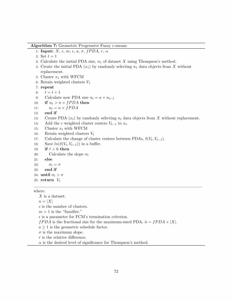
Algorithm 7: Geometric Progressive Fuzzy c-means
1: Input: X, c, m, ε, a, σ, fPDA, r, α2: Set t = 13: Calculate the initial PDA size, n1 of dataset X using Thompson’s method.4: Create the initial PDA (x1) by randomly selecting n1 data objects from X without
replacement.5: Cluster x1 with WFCM6: Retain weighted clusters V17: repeat8: t = t+ 19: Calculate new PDA size nt = a× nt−1
10: if nt > n× fPDA then11: nt = n× fPDA12: end if13: Create PDA (xt) by randomly selecting nt data objects from X without replacement.14: Add the c weighted cluster centers Vt−1 to xt.15: Cluster xt with WFCM16: Retain weighted clusters Vt17: Calculate the change of cluster centers between PDAs, δ(Vt, Vt−1).18: Save ln(δ(Vt, Vt−1)) in a buffer.19: if t > 6 then20: Calculate the slope σt21: else22: σt = σ23: end if24: until σt > σ25: return Vt
where:X is a dataset.n = |X|c is the number of clusters.m > 1 is the “fuzzifier.”ε is a parameter for FCM’s termination criterion.fPDA is the fractional size for the maximum-sized PDA, n = fPDA× |X|.a ≥ 1 is the geometric schedule factor.σ is the maximum slope.r is the relative difference.α is the desired level of significance for Thompson’s method.
72
One key principle of GOFCM is based on an observation made about SPFCM. After a number of
PDAs have been clustered, the cluster centers produced by SPFCM do not change in any appreciable
way. This is similar to Provost’s observation concerning induction algorithms [66]. Thus, GOFCM
may terminate early, without needing to process all the data.
The GOFCM algorithm follows a pattern similar to those in Gu et al. [101] and Provost [66], in
that the base algorithm selects and processes multiple samples. GOFCM also resembles algorithms
that use estimation for a better set of starting cluster centers [62] [63] [64].
Some key differences distinguish GOFCM from these similar methods. The first difference is
GOFCM’s use of Thompson’s method to derive the initial sample size. The second is that GOFCM
reuses the information from each sample (PDA). This is so because the cluster centers obtained
from a PDA are weighted, combined with the next PDA, and used as the starting cluster centers.
These differences have benefits that decrease the runtime of the algorithm. The initial cluster center
estimates are generated using the minimum amount of sampled data. The cluster center estimates
represent, using weights, all previously processed data. This reduces the number of iterations
needed by each PDA until termination [46].
In GOFCM, progressively larger samples are taken until the stopping criterion has been met.
The size of the samples is controlled by a parameter a ≥ 1, the geometric schedule factor. If a = 1,
the sample size remains constant, and the algorithm is identical to SPFCM though with a different
stopping criterion (see below). As noted in [66] [104], the actual type and rate of scheduling is a
tradeoff between cost (loss of fidelity to FCM) and benefit (speedup).
The GOFCM algorithm is also similar to eFFCM and its variants because it progressively
samples the dataset while retaining the data already sampled. As discussed above, its method of
“retaining” the data differs from eFFCM’s and mirrors SPFCM’s.
As shown in the SPFCM experiments in Chapter 4, the final cluster centers did not change very
much after the first few PDAs had been clustered. This suggested that stopping GOFCM before
all the data was clustered would improve speedup and have little impact on quality. A difficult
decision in the development of GOFCM was the stopping criterion. Provost identifies detection of
73
convergence in the context of induction algorithms as an important area of future research [66].
The same is true for clustering algorithms.
Unlike Provost’s method for induction algorithms with labeled data, there are no objective
criteria, such as model accuracy, to compare the quality of clustering algorithms. The typical
alternative method of developing a stopping criterion is to identify whenever some metric associated
with the algorithm fails to change more than a specified threshold.
The candidate metrics available for developing a stopping criterion are limited in number:
the value of the objective function, the membership values of the data examples, the amount of
data processed, the number of iterations, and the position of the cluster centers. All candidate
metrics were considered in the development of GOFCM. Thought and experimentation uncovered
considerable challenges with each.
Use of the reformulated objective function (Rm) was deemed infeasible. While the base FCM
algorithm uses an objective function, the objective function for each sample is not comparable.
One could use the reformulated objective function (Equation 2.20) for the entire dataset, but to
calculate this value would be time-consuming for a large amount of data. In fact, for large datasets
requiring accelerated algorithms, calculation of Rm would account for the majority of the runtime.
Use of membership values was also deemed infeasible. GOFCM samples the dataset without
replacement, so the PDAs have no data objects in common. GOFCM would require some other
strategy, such as comparing membership values of the initial sample of data objects across each
PDA. Regardless, such alternative strategies would be time consuming and cumbersome.
The number of iterations was considered as a stopping criterion. As mentioned above, the
number of iterations to process a PDA falls as the cluster centers’ initial starting positions approach
the final position. Assuming that GOFCM estimates cluster centers closer and closer to the final
positions as time goes on, one would expect the number of iterations to drop to a steady level.
Experiments were performed using this stopping criterion. A flaw in this technique is that the
number of iterations is an integer. Variation in the composition of the PDA can create minor
variations in the number the iterations. The number of iterations proved to be a slightly volatile
measure, resulting in different points of termination depending on initialization and random sam-
74
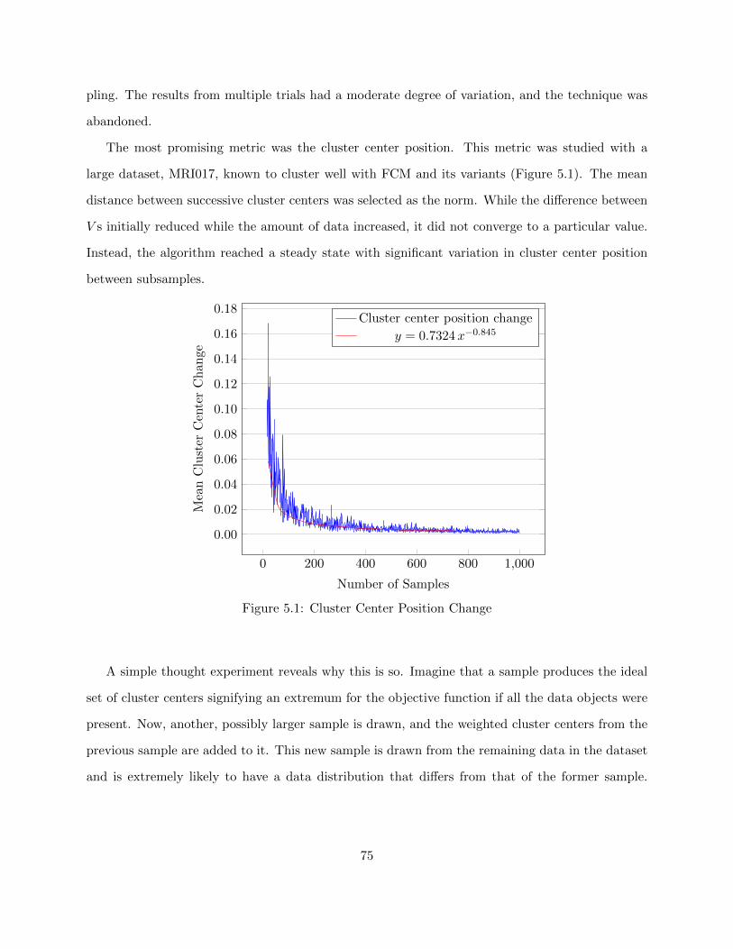
pling. The results from multiple trials had a moderate degree of variation, and the technique was
abandoned.
The most promising metric was the cluster center position. This metric was studied with a
large dataset, MRI017, known to cluster well with FCM and its variants (Figure 5.1). The mean
distance between successive cluster centers was selected as the norm. While the difference between
V s initially reduced while the amount of data increased, it did not converge to a particular value.
Instead, the algorithm reached a steady state with significant variation in cluster center position
between subsamples.
0 200 400 600 800 1,000
0.00
0.02
0.04
0.06
0.08
0.10
0.12
0.14
0.16
0.18
Number of Samples
Mea
nC
lust
erC
ente
rC
han
ge
Cluster center position change
y = 0.7324x−0.845
Figure 5.1: Cluster Center Position Change
A simple thought experiment reveals why this is so. Imagine that a sample produces the ideal
set of cluster centers signifying an extremum for the objective function if all the data objects were
present. Now, another, possibly larger sample is drawn, and the weighted cluster centers from the
previous sample are added to it. This new sample is drawn from the remaining data in the dataset
and is extremely likely to have a data distribution that differs from that of the former sample.
75
The difference in data distribution will cause the cluster centers to deviate between samples. This
condition is present for every data sample clustered.
The FCM algorithm seeks to minimize the objective function from the data that is present.
Because the distribution of the data in the samples will always be slightly different, the cluster
centers will always experience some random variation. Let us consider this random variation as
noise.
Note in Figure 5.1 that the changes in cluster centers (δ(V )) between samples are asymptotic
when noise is removed. The shape of this curve appears to be the inverse of the learning curves
noted by Provost [66] and Meek [104], but the same challenge is present: At what point in the
curve should the sampling be stopped?
If the stopping criterion is defined to be when δ(V ) falls below a user-defined value, the noise
present can be greater than the value of δ(V ). In test experiments using this criterion, a large
degree of variability was noticed in the final partitions.
Examination of the dataset and other datasets showed that this metric generally obeys the
Power Law after the first few samples. In Figure 5.1, the best fit equation, y = 0.7324x−0.845, is
plotted alongside the change in cluster centers.
In Figure 5.2, the logarithms of the x and y coordinates are plotted. Here, the best fit equation
is the straight line y = −0.845x− 0.3114. Note that ln(0.7324) = −0.3114.
Figure 5.2 provides a clear view of the noise generated by each subsample and suggests the
stopping criterion selected for GOFCM.
After each sample has been processed, the logarithm of δ(V ) is saved, and simple linear re-
gression finds the best fit equation. The best fit equation is then converted back to the original
coordinates, and the slope between the last two samples is found. The best fit line is of the form
y = ax−b, so the slope will have a range of (−∞, 0). If this slope rises above a user-defined value,
σ, GOFCM will terminate.
The selection of σ is a tradeoff between speedup and quality compared to FCM clustering the
full dataset. A small value for σ provides more speed but less quality, while a large value of σ
provides higher quality but less speed (more iterations).
76
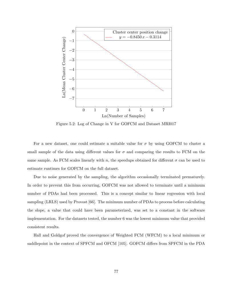
0 1 2 3 4 5 6 7
−7
−6
−5
−4
−3
−2
−1
0
Ln(Number of Samples)
Ln
(Mea
nC
lust
erC
ente
rC
han
ge)
Cluster center position changey = −0.8450x− 0.3114
Figure 5.2: Log of Change in V for GOFCM and Dataset MRI017
For a new dataset, one could estimate a suitable value for σ by using GOFCM to cluster a
small sample of the data using different values for σ and comparing the results to FCM on the
same sample. As FCM scales linearly with n, the speedups obtained for different σ can be used to
estimate runtimes for GOFCM on the full dataset.
Due to noise generated by the sampling, the algorithm occasionally terminated prematurely.
In order to prevent this from occurring, GOFCM was not allowed to terminate until a minimum
number of PDAs had been processed. This is a concept similar to linear regression with local
sampling (LRLS) used by Provost [66]. The minimum number of PDAs to process before calculating
the slope, a value that could have been parameterized, was set to a constant in the software
implementation. For the datasets tested, the number 6 was the lowest minimum value that provided
consistent results.
Hall and Goldgof proved the convergence of Weighted FCM (WFCM) to a local minimum or
saddlepoint in the context of SPFCM and OFCM [105]. GOFCM differs from SPFCM in the PDA
77
size, however the functionality of WFCM on each PDA is unchanged. Thus, GOFCM also converges
to a local minimum or saddlepoint.
GOFCM also differs from SPFCM in that its stopping criterion typically halts GOFCM before
the entire dataset is clustered. Each PDA clustered by WFCM still converges, and the use of an
“early” stopping criterion is analogous to a scenario in which the data clustered by GOFCM is all
the data that is available.
A related issue is how well the overall stopping criterion would function if GOFCM were applied
to streaming data. The GOFCM algorithm, as defined, draws random samples from the dataset.
In a streaming scenario, the incoming data might not be randomly distributed, nor proportionally
represent the whole dataset. In these cases, the stopping criterion might not cause the selection of
subsets to cluster to cease.
To see how the stopping criterion might work in another setting, I applied it to SPFCM, also.
The assumption was that it would save time at the cost of leaving some of the data unused. See
Section 5.5 for details.
5.4 The MSERFCM Algorithm
Minimum Sample Estimate Random Fuzzy C-Means (MSERFCM) was designed as an improve-
ment to rseFCM. It is similar to, but much simpler than, methods that try to find a better set of
starting cluster centers [62] [63] [64]. Algorithm 8 presents a detailed description of MSERFCM.
The rseFCM algorithm uses c randomly selected data objects as initial cluster centers. In
contrast, MSERFCM processes a sample of the dataset to estimate initial cluster centers. This
is the only major difference between rseFCM and MSERFCM, unless one of the assumptions (see
below) is violated.
For a dataset, X of size n, the minimum size of a sample, n1, is estimated using Thompson’s
method. A sample, x1 of size n1, is drawn without replacement from the dataset and clustered
by FCM. The positions of the cluster centers, V1, produced by FCM are saved. Then a second
sample, x2, is drawn from X. This second sample size is user-specified. The amount of available
random access memory (RAM) in the computing environment or some other practical concern may
78
influence the choice of the second sample size. In the software implementation of MSERFCM, the
user-specified sample size, n2 = |x2|, is defined as fPDA×n, which happens to be the same sample
size used by rseFCM. The previously saved cluster center positions, V1, are used to initialize FCM
to cluster x2.
The MSERFCM algorithm assumes that the estimated sample size, n1, is less than both the
specified sample size, n2, and the total dataset size, n: n1 < n2 < n. This assumption may not be
correct when Thompson’s method estimates a large value for n1. If this occurs, MSERFCM will
be less efficient than rseFCM. To correct this, the following adjustments were made.
When n2 < n1 < n, the estimated sample size exceeds the user-specified sample size and
MSERFCM degenerates to rseFCM with a sample of size n1. When n2 < n < n1, the estimated
sample size exceeds the available data, and MSERFCM degenerates to FCM, processing the entire
dataset. In both of the latter cases, the sample can exceed the available RAM which would provide
the actual limit.
5.4.1 Runtime Complexity
MSERFCM has an expected runtime complexity of O(n2i2sc + n1i1sc), due to two successive
applications of FCM (Section 2.2.2.1). The rseFCM algorithm has an expected runtime complexity
of O(n2isc). In practice, MSERFCM usually has a shorter runtime than rseFCM, because of the
improved set of starting clusters which reduce i2 to compensate more than enough for the additional
O(n1i1sc) time.
5.5 The MODSPFCM Algorithm
Modified Single Pass Fuzzy c-means (MODSPFCM) is identical to SPFCM except for the stop-
ping criterion. If the conditions for the stopping criterion designed for GOFCM (Section 5.3) are
met, MODSPFCM will terminate immediately. MODSPFCM converges to a local minimum or
saddlepoint in the same manner as GOFCM [105]. MODSPFCM is formally described as follows:
79
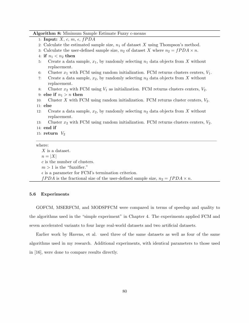
Algorithm 8: Minimum Sample Estimate Fuzzy c-means
1: Input: X, c, m, ε, fPDA2: Calculate the estimated sample size, n1 of dataset X using Thompson’s method.3: Calculate the user-defined sample size, n2 of dataset X where n2 = fPDA× n.4: if n1 < n2 then5: Create a data sample, x1, by randomly selecting n1 data objects from X without
replacement.6: Cluster x1 with FCM using random initialization. FCM returns clusters centers, V1.7: Create a data sample, x2, by randomly selecting n2 data objects from X without
replacement.8: Cluster x2 with FCM using V1 as initialization. FCM returns clusters centers, V2.9: else if n1 > n then
10: Cluster X with FCM using random initialization. FCM returns cluster centers, V2.11: else12: Create a data sample, x2, by randomly selecting n2 data objects from X without
replacement.13: Cluster x2 with FCM using random initialization. FCM returns clusters centers, V2.14: end if15: return V2
where:X is a dataset.n = |X|c is the number of clusters.m > 1 is the “fuzzifier.”ε is a parameter for FCM’s termination criterion.fPDA is the fractional size of the user-defined sample size, n2 = fPDA× n.
5.6 Experiments
GOFCM, MSERFCM, and MODSPFCM were compared in terms of speedup and quality to
the algorithms used in the “simple experiment” in Chapter 4. The experiments applied FCM and
seven accelerated variants to four large real-world datasets and two artificial datasets.
Earlier work by Havens, et al. used three of the same datasets as well as four of the same
algorithms used in my research. Additional experiments, with identical parameters to those used
in [16], were done to compare results directly.
80

Algorithm 9: Modified Single Pass Fuzzy c-means
1: Input: X, c, m, ε, σ, fPDA2: Set t = 13: Calculate the PDA size, n = n× fPDA4: Create the initial PDA (x1) by randomly selecting n data objects from X without
replacement.5: Cluster x1 with WFCM6: Retain weighted clusters V17: repeat8: t = t+ 19: Create PDA (xt) by randomly selecting n data objects from X without replacement.
10: Add the c weighted cluster centers Vt−1 to xt.11: Cluster xt with WFCM12: Retain weighted clusters Vt13: Calculate the change of cluster centers between PDAs, δ(Vt, Vt−1).14: Save ln(δ(Vt, Vt−1)) in a buffer.15: if t > 6 then16: Calculate the slope σt17: else18: σt = σ19: end if20: until σt > σ21: return Vt
where:X is a dataset.n = |X|.c is the number of clusters.m > 1 is the “fuzzifier.”ε is a parameter for FCM’s termination criterion.fPDA is the fractional size for the maximum-sized PDA, n = fPDA× |X|.σ is the maximum slope.
5.6.1 Experimental Procedures
Three sets of experiments were performed. The main experiment compared GOFCM and
MSERFCM to algorithms previously compared in Chapter 4. A second experiment mirrored work
performed by Havens [16]. A third, smaller experiment, compared MODSPFCM to related algo-
rithms.
The experimental procedures, except where noted, were identical to those described in Chapter
4. To recount, the cluster centers predicted by the FCM family vary based on the initial set of
81
cluster centers, V . Therefore, initialization for all algorithms was performed by randomly selecting
c data objects in the dataset, X, as the initial values of V . Each experiment consisted of 30 trials
to ensure a statistically significant sample. While the initialization for each trial of an experiment
was different, the same set of 30 initializations was used for each algorithm in the experimentation.
The average values over 30 trials were recorded for their runtime and quality metrics.
All algorithms except for FCM and OFCM assume that the data is in random order, or the
implementation performs random sampling. In these experiments (excepting for FCM and OFCM),
the entire dataset was randomized before processing each trial using the procedure described in
A.2. In addition to recording the runtime of the algorithm, the software implementation separately
recorded the time taken to sample the data randomly, as well as the time taken to perform I/O.
Unless otherwise noted, reported times and speedup comparisons include the runtimes for both
randomization and I/O. The quality and fidelity metrics DQRm%, CC%, and ARI were recorded.
The main experiment compared the algorithms FCM, SPFCM, OFCM, eFFCM, rseFCM,
GOFCM, and MSERFCM. Different datasets were used than those in Chapter 4. The Pendig-
its and Landsat datasets were not used because of their small size. The main experiment used the
MRI datasets, MRI016, MRI017, and MRI018, a challenging real-world dataset of plankton images,
PLK01, and two artificial datasets, D6C5 and D10C7. Details about these datasets are in Chapter
3.
The second experiment was modeled on an experiment in Havens’s work, “Fuzzy c-Means Al-
gorithms for Very Large Data” [16]. Conveniently, his experiments clustered rseFCM, SPFCM,
and OFCM using the same MRI datasets as in my research. His experiments differed in several
ways. Only 21 trials were performed, the fuzzifier was set to 1.7, and the termination criterion was
changed to use the maximum change in V . Havens reports results for SU and ARI; these were
rounded to nearest whole number and two decimal digits respectively.
His algorithm implementation was done in MATLAB rather than in a Linux/C implementation.
Havens pre-randomized the files and did not count that step in the algorithm execution time, but
he did consider sampling and I/O time [106]. As noted in Chapter 4, the experiments and software
implementation reported the time spent to randomize the files and to perform I/O in the algorithm
82
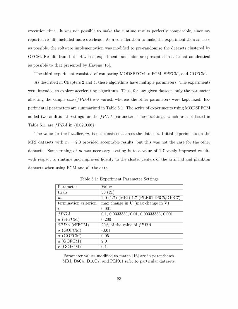
execution time. It was not possible to make the runtime results perfectly comparable, since my
reported results included more overhead. As a consideration to make the experimentation as close
as possible, the software implementation was modified to pre-randomize the datasets clustered by
OFCM. Results from both Havens’s experiments and mine are presented in a format as identical
as possible to that presented by Havens [16].
The third experiment consisted of comparing MODSPFCM to FCM, SPFCM, and GOFCM.
As described in Chapters 2 and 4, these algorithms have multiple parameters. The experiments
were intended to explore accelerating algorithms. Thus, for any given dataset, only the parameter
affecting the sample size (fPDA) was varied, whereas the other parameters were kept fixed. Ex-
perimental parameters are summarized in Table 5.1. The series of experiments using MODSPFCM
added two additional settings for the fPDA parameter. These settings, which are not listed in
Table 5.1, are fPDA in {0.02,0.06}.
The value for the fuzzifier, m, is not consistent across the datasets. Initial experiments on the
MRI datasets with m = 2.0 provided acceptable results, but this was not the case for the other
datasets. Some tuning of m was necessary; setting it to a value of 1.7 vastly improved results
with respect to runtime and improved fidelity to the cluster centers of the artificial and plankton
datasets when using FCM and all the data.
Table 5.1: Experiment Parameter Settings
Parameter Value
trials 30 (21)
m 2.0 (1.7) (MRI) 1.7 (PLK01,D6C5,D10C7)
termination criterion max change in U (max change in V)
ε 0.001
fPDA 0.1, 0.0333333, 0.01, 0.00333333, 0.001
α (eFFCM) 0.200
δPDA (eFFCM) 20% of the value of fPDA
σ (GOFCM) -0.01
α (GOFCM) 0.05
a (GOFCM) 2.0
r (GOFCM) 0.1
Parameter values modified to match [16] are in parentheses.MRI, D6C5, D10C7, and PLK01 refer to particular datasets.
83
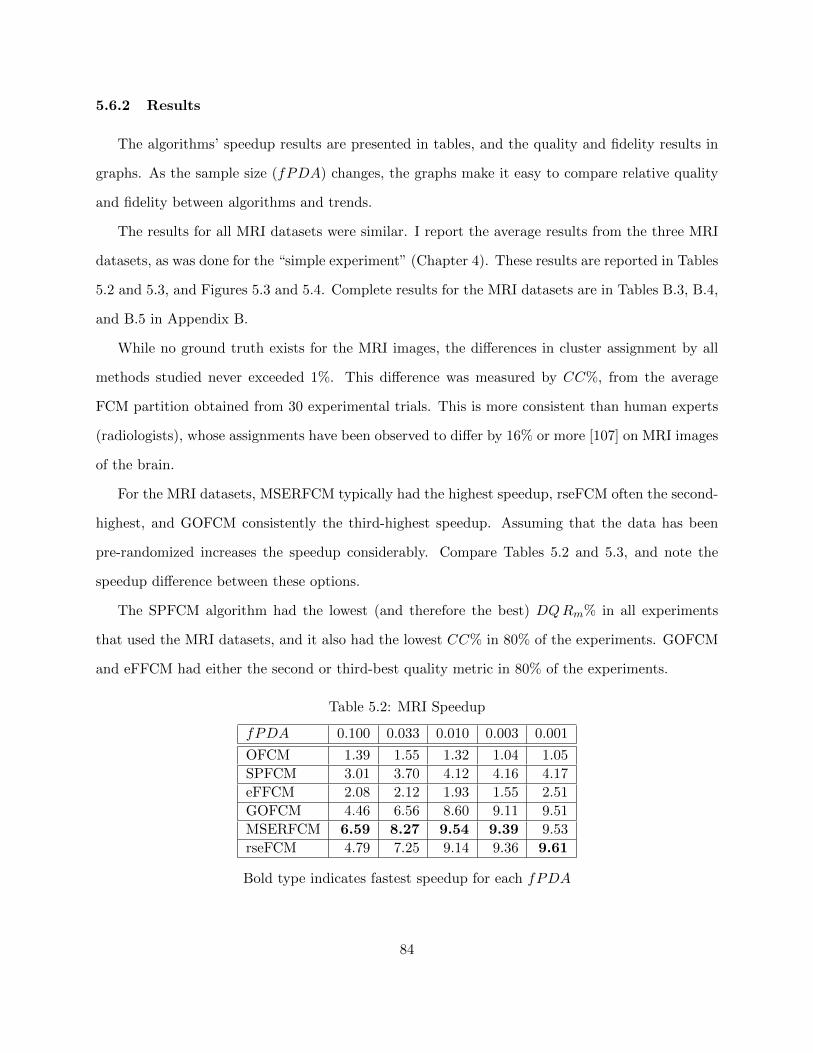
5.6.2 Results
The algorithms’ speedup results are presented in tables, and the quality and fidelity results in
graphs. As the sample size (fPDA) changes, the graphs make it easy to compare relative quality
and fidelity between algorithms and trends.
The results for all MRI datasets were similar. I report the average results from the three MRI
datasets, as was done for the “simple experiment” (Chapter 4). These results are reported in Tables
5.2 and 5.3, and Figures 5.3 and 5.4. Complete results for the MRI datasets are in Tables B.3, B.4,
and B.5 in Appendix B.
While no ground truth exists for the MRI images, the differences in cluster assignment by all
methods studied never exceeded 1%. This difference was measured by CC%, from the average
FCM partition obtained from 30 experimental trials. This is more consistent than human experts
(radiologists), whose assignments have been observed to differ by 16% or more [107] on MRI images
of the brain.
For the MRI datasets, MSERFCM typically had the highest speedup, rseFCM often the second-
highest, and GOFCM consistently the third-highest speedup. Assuming that the data has been
pre-randomized increases the speedup considerably. Compare Tables 5.2 and 5.3, and note the
speedup difference between these options.
The SPFCM algorithm had the lowest (and therefore the best) DQRm% in all experiments
that used the MRI datasets, and it also had the lowest CC% in 80% of the experiments. GOFCM
and eFFCM had either the second or third-best quality metric in 80% of the experiments.
Table 5.2: MRI Speedup
fPDA 0.100 0.033 0.010 0.003 0.001
OFCM 1.39 1.55 1.32 1.04 1.05
SPFCM 3.01 3.70 4.12 4.16 4.17
eFFCM 2.08 2.12 1.93 1.55 2.51
GOFCM 4.46 6.56 8.60 9.11 9.51
MSERFCM 6.59 8.27 9.54 9.39 9.53
rseFCM 4.79 7.25 9.14 9.36 9.61
Bold type indicates fastest speedup for each fPDA
84
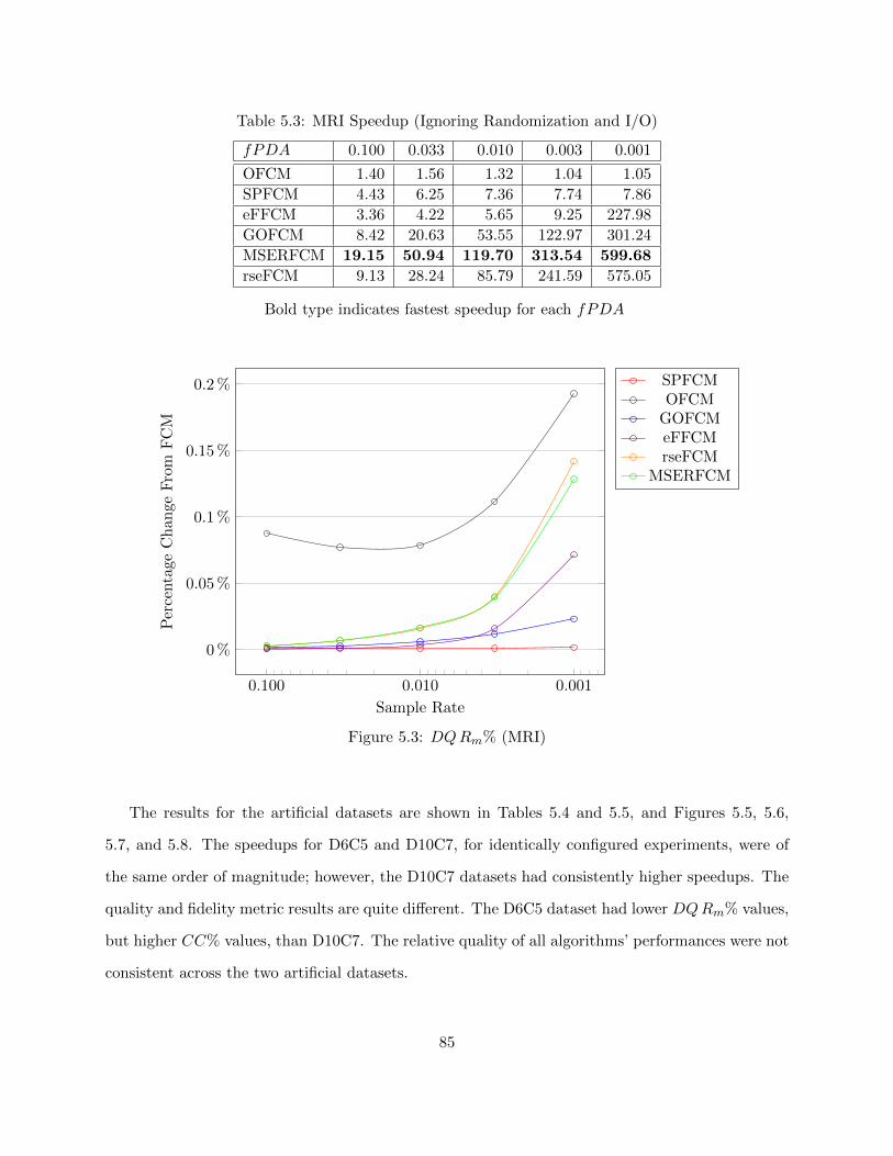
Table 5.3: MRI Speedup (Ignoring Randomization and I/O)
fPDA 0.100 0.033 0.010 0.003 0.001
OFCM 1.40 1.56 1.32 1.04 1.05
SPFCM 4.43 6.25 7.36 7.74 7.86
eFFCM 3.36 4.22 5.65 9.25 227.98
GOFCM 8.42 20.63 53.55 122.97 301.24
MSERFCM 19.15 50.94 119.70 313.54 599.68
rseFCM 9.13 28.24 85.79 241.59 575.05
Bold type indicates fastest speedup for each fPDA
0.0010.0100.100
0 %
0.05 %
0.1 %
0.15 %
0.2 %
Sample Rate
Per
centa
geC
han
geF
rom
FC
M
SPFCMOFCM
GOFCMeFFCMrseFCM
MSERFCM
Figure 5.3: DQRm% (MRI)
The results for the artificial datasets are shown in Tables 5.4 and 5.5, and Figures 5.5, 5.6,
5.7, and 5.8. The speedups for D6C5 and D10C7, for identically configured experiments, were of
the same order of magnitude; however, the D10C7 datasets had consistently higher speedups. The
quality and fidelity metric results are quite different. The D6C5 dataset had lower DQRm% values,
but higher CC% values, than D10C7. The relative quality of all algorithms’ performances were not
consistent across the two artificial datasets.
85
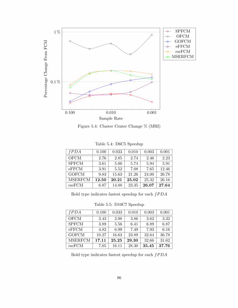
0.0010.0100.100
0.1 %
1 %
Sample Rate
Per
centa
geC
han
geF
rom
FC
M
SPFCMOFCM
GOFCMeFFCMrseFCM
MSERFCM
Figure 5.4: Cluster Center Change % (MRI)
Table 5.4: D6C5 Speedup
fPDA 0.100 0.033 0.010 0.003 0.001
OFCM 2.76 2.85 2.74 2.46 2.23
SPFCM 3.61 5.00 5.74 5.94 5.91
eFFCM 3.91 5.52 7.08 7.65 12.46
GOFCM 9.83 15.63 21.26 24.00 26.78
MSERFCM 12.50 20.21 25.02 25.32 26.16
rseFCM 6.87 14.88 23.35 26.07 27.64
Bold type indicates fastest speedup for each fPDA
Table 5.5: D10C7 Speedup
fPDA 0.100 0.033 0.010 0.003 0.001
OFCM 3.43 3.98 3.86 3.62 3.32
SPFCM 3.89 5.56 6.41 6.89 6.87
eFFCM 4.82 6.99 7.49 7.93 6.16
GOFCM 10.27 16.63 23.89 32.64 36.78
MSERFCM 17.11 25.25 29.30 32.66 31.62
rseFCM 7.05 16.11 28.30 35.45 37.76
Bold type indicates fastest speedup for each fPDA
86
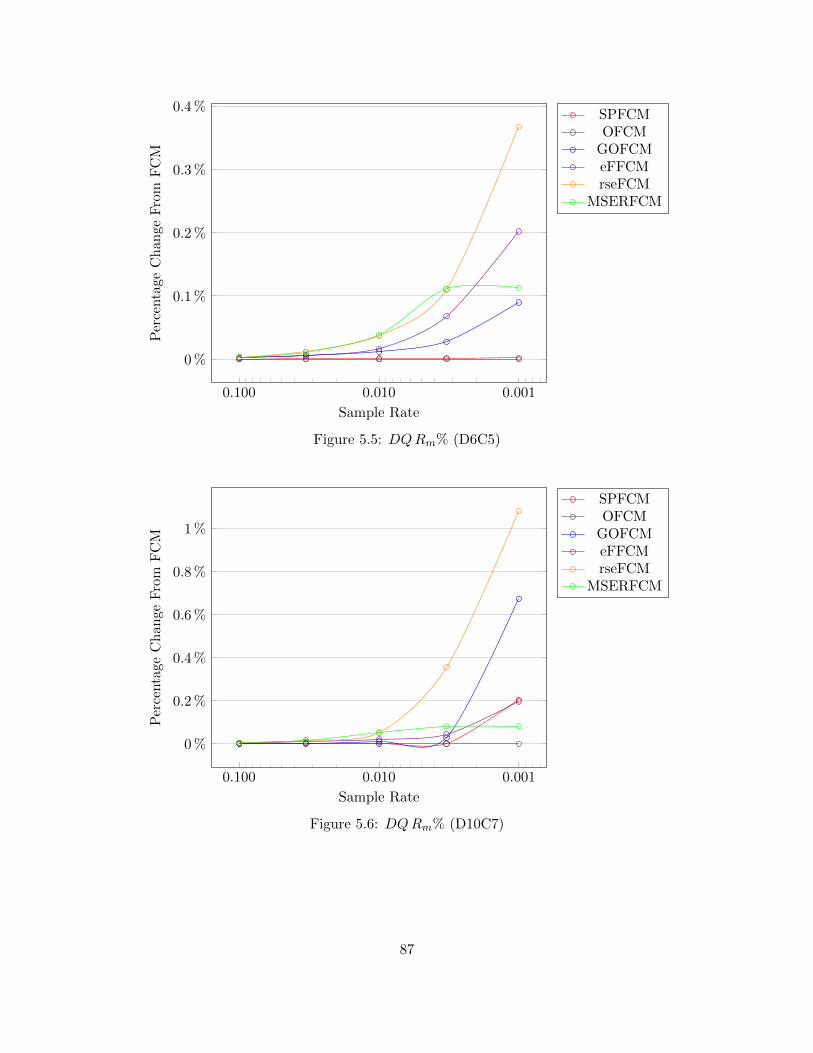
0.0010.0100.100
0 %
0.1 %
0.2 %
0.3 %
0.4 %
Sample Rate
Per
centa
geC
han
geF
rom
FC
M
SPFCMOFCM
GOFCMeFFCMrseFCM
MSERFCM
Figure 5.5: DQRm% (D6C5)
0.0010.0100.100
0 %
0.2 %
0.4 %
0.6 %
0.8 %
1 %
Sample Rate
Per
centa
geC
han
geF
rom
FC
M
SPFCMOFCM
GOFCMeFFCMrseFCM
MSERFCM
Figure 5.6: DQRm% (D10C7)
87
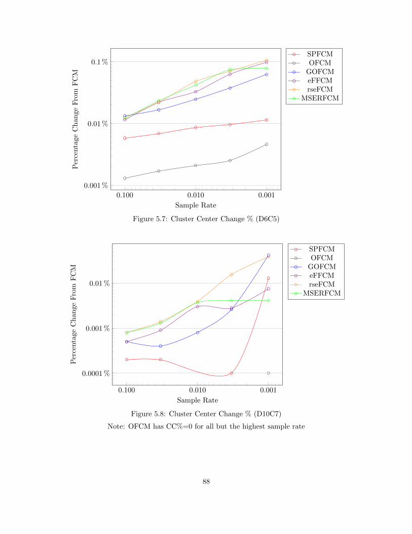
0.0010.0100.100
0.001 %
0.01 %
0.1 %
Sample Rate
Per
centa
ge
Ch
an
ge
Fro
mF
CM
SPFCMOFCM
GOFCMeFFCMrseFCM
MSERFCM
Figure 5.7: Cluster Center Change % (D6C5)
0.0010.0100.100
0.0001 %
0.001 %
0.01 %
Sample Rate
Per
centa
geC
han
geF
rom
FC
M
SPFCMOFCM
GOFCMeFFCMrseFCM
MSERFCM
Figure 5.8: Cluster Center Change % (D10C7)
Note: OFCM has CC%=0 for all but the highest sample rate
88
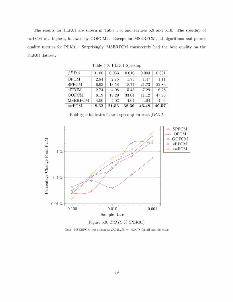
The results for PLK01 are shown in Table 5.6, and Figures 5.9 and 5.10. The speedup of
rseFCM was highest, followed by GOFCM’s. Except for MSERFCM, all algorithms had poorer
quality metrics for PLK01. Surprisingly, MSERFCM consistently had the best quality on the
PLK01 dataset.
Table 5.6: PLK01 Speedup
fPDA 0.100 0.033 0.010 0.003 0.001
OFCM 2.84 2.75 1.75 1.47 1.11
SPFCM 6.93 13.58 18.77 21.73 22.83
eFFCM 2.74 4.08 5.45 7.29 6.28
GOFCM 8.19 18.29 33.04 41.12 47.95
MSERFCM 4.00 4.03 4.04 4.04 4.04
rseFCM 8.52 21.55 38.39 46.48 49.57
Bold type indicates fastest speedup for each fPDA
0.0010.0100.1000.01 %
0.1 %
1 %
Sample Rate
Per
centa
geC
han
geF
rom
FC
M
SPFCMOFCM
GOFCMeFFCMrseFCM
Figure 5.9: DQRm% (PLK01)
Note: MSERFCM not shown as DQRm% = −0.0078 for all sample rates
89
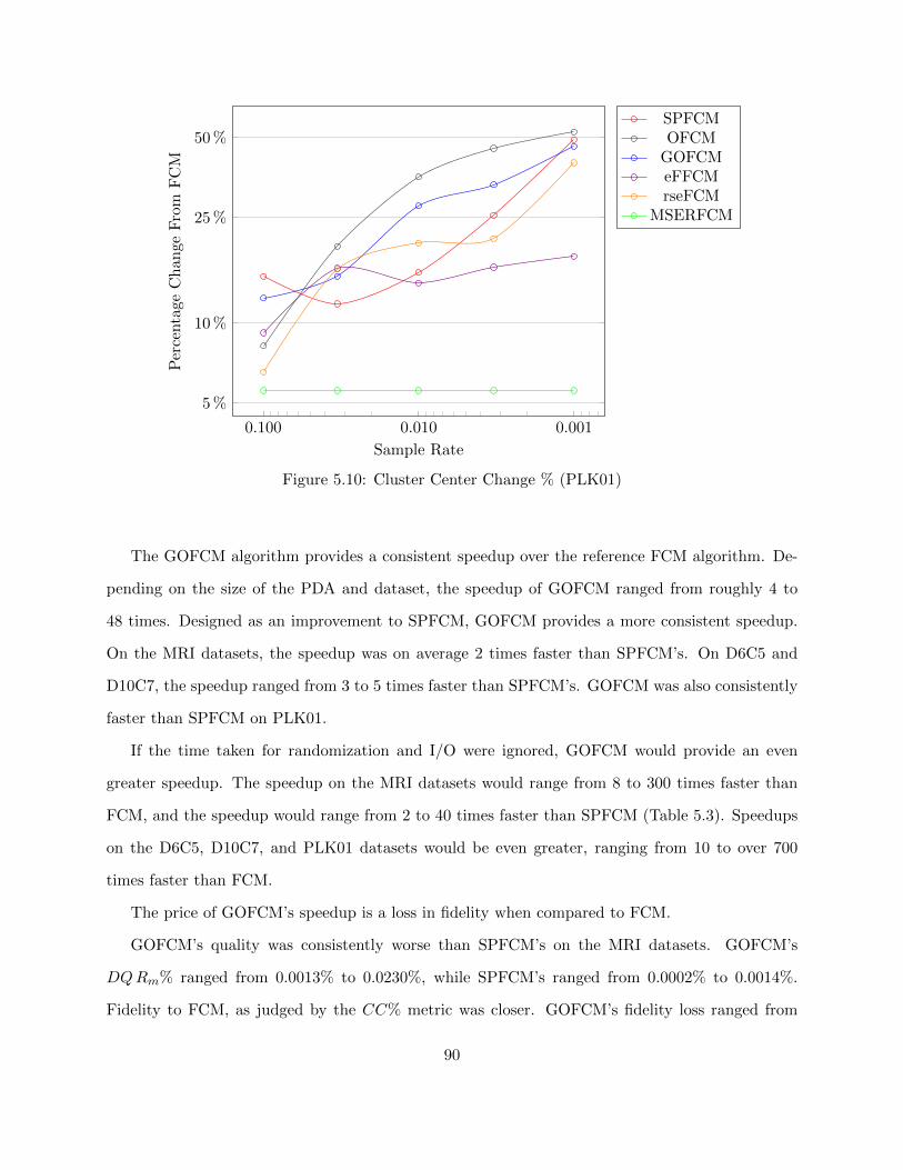
0.0010.0100.100
5 %
10 %
25 %
50 %
Sample Rate
Per
centa
geC
han
geF
rom
FC
M
SPFCMOFCM
GOFCMeFFCMrseFCM
MSERFCM
Figure 5.10: Cluster Center Change % (PLK01)
The GOFCM algorithm provides a consistent speedup over the reference FCM algorithm. De-
pending on the size of the PDA and dataset, the speedup of GOFCM ranged from roughly 4 to
48 times. Designed as an improvement to SPFCM, GOFCM provides a more consistent speedup.
On the MRI datasets, the speedup was on average 2 times faster than SPFCM’s. On D6C5 and
D10C7, the speedup ranged from 3 to 5 times faster than SPFCM’s. GOFCM was also consistently
faster than SPFCM on PLK01.
If the time taken for randomization and I/O were ignored, GOFCM would provide an even
greater speedup. The speedup on the MRI datasets would range from 8 to 300 times faster than
FCM, and the speedup would range from 2 to 40 times faster than SPFCM (Table 5.3). Speedups
on the D6C5, D10C7, and PLK01 datasets would be even greater, ranging from 10 to over 700
times faster than FCM.
The price of GOFCM’s speedup is a loss in fidelity when compared to FCM.
GOFCM’s quality was consistently worse than SPFCM’s on the MRI datasets. GOFCM’s
DQRm% ranged from 0.0013% to 0.0230%, while SPFCM’s ranged from 0.0002% to 0.0014%.
Fidelity to FCM, as judged by the CC% metric was closer. GOFCM’s fidelity loss ranged from
90
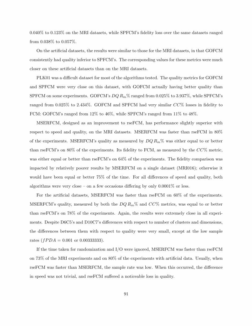
0.040% to 0.123% on the MRI datasets, while SPFCM’s fidelity loss over the same datasets ranged
from 0.038% to 0.057%.
On the artificial datasets, the results were similar to those for the MRI datasets, in that GOFCM
consistently had quality inferior to SPFCM’s. The corresponding values for these metrics were much
closer on these artificial datasets than on the MRI datasets.
PLK01 was a difficult dataset for most of the algorithms tested. The quality metrics for GOFCM
and SPFCM were very close on this dataset, with GOFCM actually having better quality than
SPFCM on some experiments. GOFCM’s DQRm% ranged from 0.025% to 3.937%, while SPFCM’s
ranged from 0.025% to 2.434%. GOFCM and SPFCM had very similar CC% losses in fidelity to
FCM: GOFCM’s ranged from 12% to 46%, while SPFCM’s ranged from 11% to 48%.
MSERFCM, designed as an improvement to rseFCM, has performance slightly superior with
respect to speed and quality, on the MRI datasets. MSERFCM was faster than rseFCM in 80%
of the experiments. MSERFCM’s quality as measured by DQRm% was either equal to or better
than rseFCM’s on 80% of the experiments. Its fidelity to FCM, as measured by the CC% metric,
was either equal or better than rseFCM’s on 64% of the experiments. The fidelity comparison was
impacted by relatively poorer results by MSERFCM on a single dataset (MRI016); otherwise it
would have been equal or better 75% of the time. For all differences of speed and quality, both
algorithms were very close – on a few occasions differing by only 0.0001% or less.
For the artificial datasets, MSERFCM was faster than rseFCM on 60% of the experiments.
MSERFCM’s quality, measured by both the DQRm% and CC% metrics, was equal to or better
than rseFCM’s on 78% of the experiments. Again, the results were extremely close in all experi-
ments. Despite D6C5’s and D10C7’s differences with respect to number of clusters and dimensions,
the differences between them with respect to quality were very small, except at the low sample
rates (fPDA = 0.001 or 0.00333333).
If the time taken for randomization and I/O were ignored, MSERFCM was faster than rseFCM
on 73% of the MRI experiments and on 80% of the experiments with artificial data. Usually, when
rseFCM was faster than MSERFCM, the sample rate was low. When this occurred, the difference
in speed was not trivial, and rseFCM suffered a noticeable loss in quality.
91
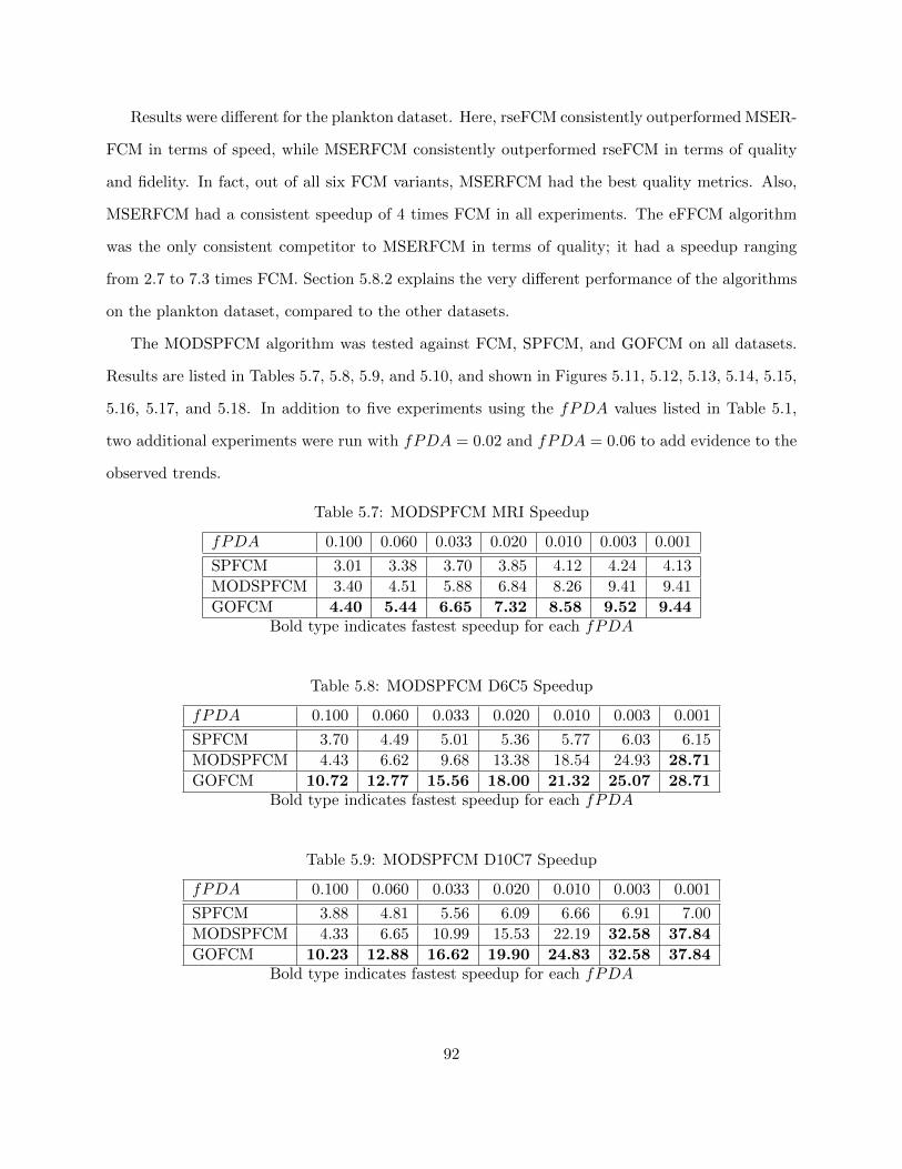
Results were different for the plankton dataset. Here, rseFCM consistently outperformed MSER-
FCM in terms of speed, while MSERFCM consistently outperformed rseFCM in terms of quality
and fidelity. In fact, out of all six FCM variants, MSERFCM had the best quality metrics. Also,
MSERFCM had a consistent speedup of 4 times FCM in all experiments. The eFFCM algorithm
was the only consistent competitor to MSERFCM in terms of quality; it had a speedup ranging
from 2.7 to 7.3 times FCM. Section 5.8.2 explains the very different performance of the algorithms
on the plankton dataset, compared to the other datasets.
The MODSPFCM algorithm was tested against FCM, SPFCM, and GOFCM on all datasets.
Results are listed in Tables 5.7, 5.8, 5.9, and 5.10, and shown in Figures 5.11, 5.12, 5.13, 5.14, 5.15,
5.16, 5.17, and 5.18. In addition to five experiments using the fPDA values listed in Table 5.1,
two additional experiments were run with fPDA = 0.02 and fPDA = 0.06 to add evidence to the
observed trends.
Table 5.7: MODSPFCM MRI Speedup
fPDA 0.100 0.060 0.033 0.020 0.010 0.003 0.001
SPFCM 3.01 3.38 3.70 3.85 4.12 4.24 4.13
MODSPFCM 3.40 4.51 5.88 6.84 8.26 9.41 9.41
GOFCM 4.40 5.44 6.65 7.32 8.58 9.52 9.44Bold type indicates fastest speedup for each fPDA
Table 5.8: MODSPFCM D6C5 Speedup
fPDA 0.100 0.060 0.033 0.020 0.010 0.003 0.001
SPFCM 3.70 4.49 5.01 5.36 5.77 6.03 6.15
MODSPFCM 4.43 6.62 9.68 13.38 18.54 24.93 28.71
GOFCM 10.72 12.77 15.56 18.00 21.32 25.07 28.71Bold type indicates fastest speedup for each fPDA
Table 5.9: MODSPFCM D10C7 Speedup
fPDA 0.100 0.060 0.033 0.020 0.010 0.003 0.001
SPFCM 3.88 4.81 5.56 6.09 6.66 6.91 7.00
MODSPFCM 4.33 6.65 10.99 15.53 22.19 32.58 37.84
GOFCM 10.23 12.88 16.62 19.90 24.83 32.58 37.84Bold type indicates fastest speedup for each fPDA
92
Table 5.10: MODSPFCM PLK01 Speedup
fPDA 0.100 0.060 0.033 0.020 0.010 0.003 0.001
SPFCM 6.98 9.86 13.88 16.63 18.80 22.15 23.75
MODSPFCM 8.31 11.60 18.77 25.13 33.46 42.92 51.27
GOFCM 8.31 11.58 18.80 25.09 33.45 42.92 51.28Bold type indicates fastest speedup for each fPDA
0.0010.0100.100
0 %
0.005 %
0.01 %
0.015 %
0.02 %
0.025 %
Sample Rate
Per
centa
geC
han
geF
rom
FC
M
SPFCMMODSPFCM
GOFCM
Figure 5.11: DQRm% (MRI)
The speedup of MODSPFCM generally fell between those of SPFCM and GOFCM. On three
occasions, MODSPFCM was slightly faster than GOFCM on PLK01 by a very narrow margin.
Statistical significance was tested for, on the largest of these speed differences, using a one-tailed
Welch’s t-test. The t-test returned t = 0.025 with 58 d.f. This corresponds to p = 0.4901, which is
not considered statistically significant.
The quality of MODSPFCM, as measured by DQRm% also falls between that of the other
two algorithms. In the smallest two sample rates for D10C7 and all sample rates for PLK01, the
DQRm% values for MODSPFCM and GOFCM were identical. In these cases, the estimated sample
size exceeded the limits set by fPDA, and GOFCM “degenerated” to MODSPFCM.
93
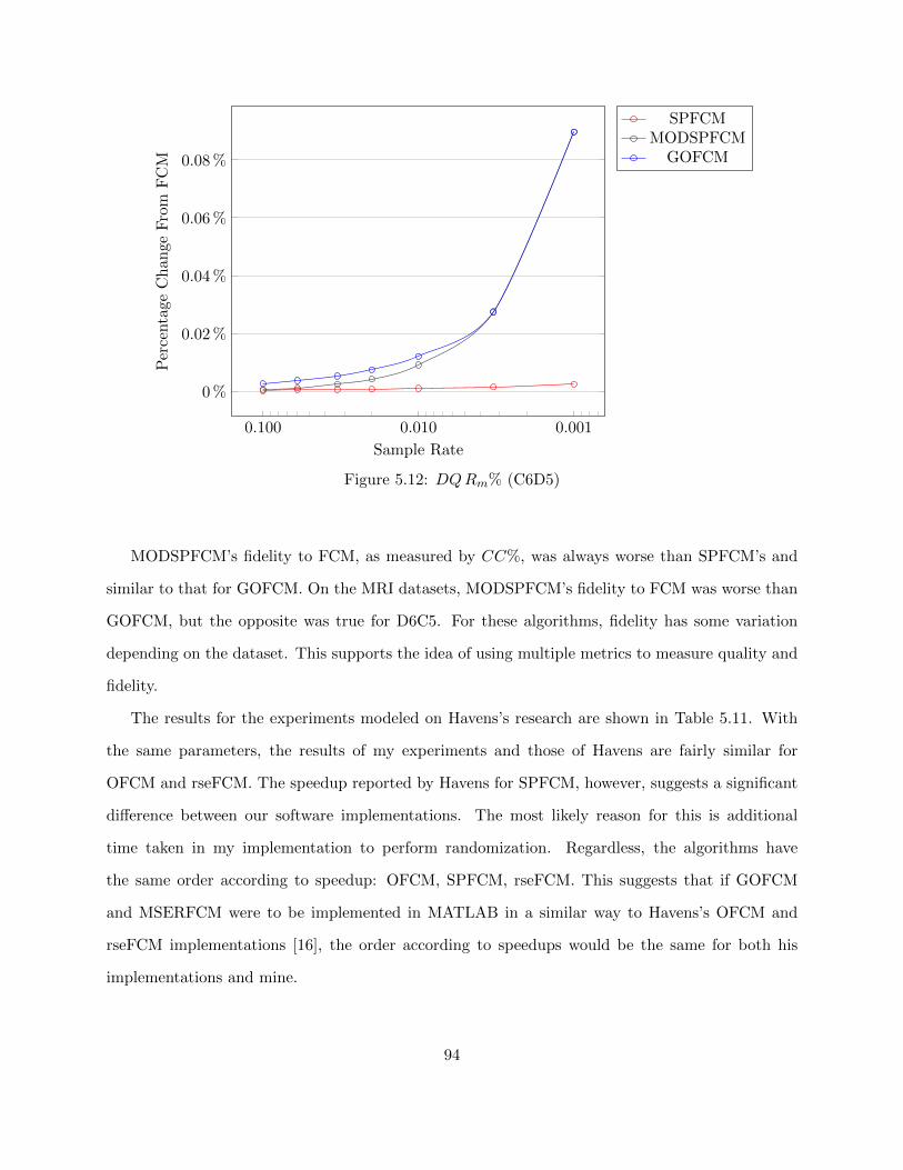
0.0010.0100.100
0 %
0.02 %
0.04 %
0.06 %
0.08 %
Sample Rate
Per
centa
geC
han
geF
rom
FC
M
SPFCMMODSPFCM
GOFCM
Figure 5.12: DQRm% (C6D5)
MODSPFCM’s fidelity to FCM, as measured by CC%, was always worse than SPFCM’s and
similar to that for GOFCM. On the MRI datasets, MODSPFCM’s fidelity to FCM was worse than
GOFCM, but the opposite was true for D6C5. For these algorithms, fidelity has some variation
depending on the dataset. This supports the idea of using multiple metrics to measure quality and
fidelity.
The results for the experiments modeled on Havens’s research are shown in Table 5.11. With
the same parameters, the results of my experiments and those of Havens are fairly similar for
OFCM and rseFCM. The speedup reported by Havens for SPFCM, however, suggests a significant
difference between our software implementations. The most likely reason for this is additional
time taken in my implementation to perform randomization. Regardless, the algorithms have
the same order according to speedup: OFCM, SPFCM, rseFCM. This suggests that if GOFCM
and MSERFCM were to be implemented in MATLAB in a similar way to Havens’s OFCM and
rseFCM implementations [16], the order according to speedups would be the same for both his
implementations and mine.
94
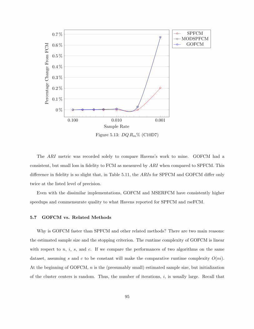
0.0010.0100.100
0 %
0.1 %
0.2 %
0.3 %
0.4 %
0.5 %
0.6 %
0.7 %
Sample Rate
Per
centa
geC
han
geF
rom
FC
M
SPFCMMODSPFCM
GOFCM
Figure 5.13: DQRm% (C10D7)
The ARI metric was recorded solely to compare Havens’s work to mine. GOFCM had a
consistent, but small loss in fidelity to FCM as measured by ARI when compared to SPFCM. This
difference in fidelity is so slight that, in Table 5.11, the ARIs for SPFCM and GOFCM differ only
twice at the listed level of precision.
Even with the dissimilar implementations, GOFCM and MSERFCM have consistently higher
speedups and commensurate quality to what Havens reported for SPFCM and rseFCM.
5.7 GOFCM vs. Related Methods
Why is GOFCM faster than SPFCM and other related methods? There are two main reasons:
the estimated sample size and the stopping criterion. The runtime complexity of GOFCM is linear
with respect to n, i, s, and c. If we compare the performances of two algorithms on the same
dataset, assuming s and c to be constant will make the comparative runtime complexity O(ni).
At the beginning of GOFCM, n is the (presumably small) estimated sample size, but initialization
of the cluster centers is random. Thus, the number of iterations, i, is usually large. Recall that
95
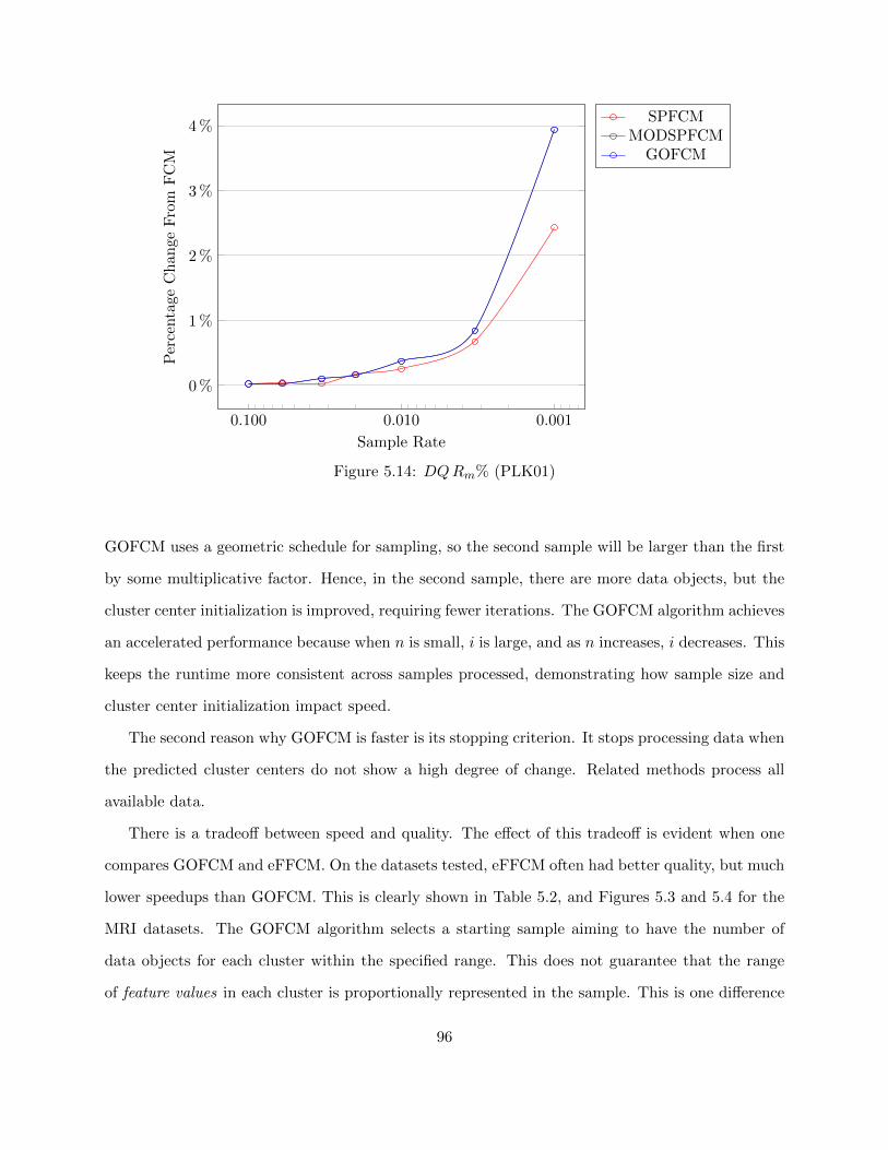
0.0010.0100.100
0 %
1 %
2 %
3 %
4 %
Sample Rate
Per
centa
geC
han
geF
rom
FC
M
SPFCMMODSPFCM
GOFCM
Figure 5.14: DQRm% (PLK01)
GOFCM uses a geometric schedule for sampling, so the second sample will be larger than the first
by some multiplicative factor. Hence, in the second sample, there are more data objects, but the
cluster center initialization is improved, requiring fewer iterations. The GOFCM algorithm achieves
an accelerated performance because when n is small, i is large, and as n increases, i decreases. This
keeps the runtime more consistent across samples processed, demonstrating how sample size and
cluster center initialization impact speed.
The second reason why GOFCM is faster is its stopping criterion. It stops processing data when
the predicted cluster centers do not show a high degree of change. Related methods process all
available data.
There is a tradeoff between speed and quality. The effect of this tradeoff is evident when one
compares GOFCM and eFFCM. On the datasets tested, eFFCM often had better quality, but much
lower speedups than GOFCM. This is clearly shown in Table 5.2, and Figures 5.3 and 5.4 for the
MRI datasets. The GOFCM algorithm selects a starting sample aiming to have the number of
data objects for each cluster within the specified range. This does not guarantee that the range
of feature values in each cluster is proportionally represented in the sample. This is one difference
96
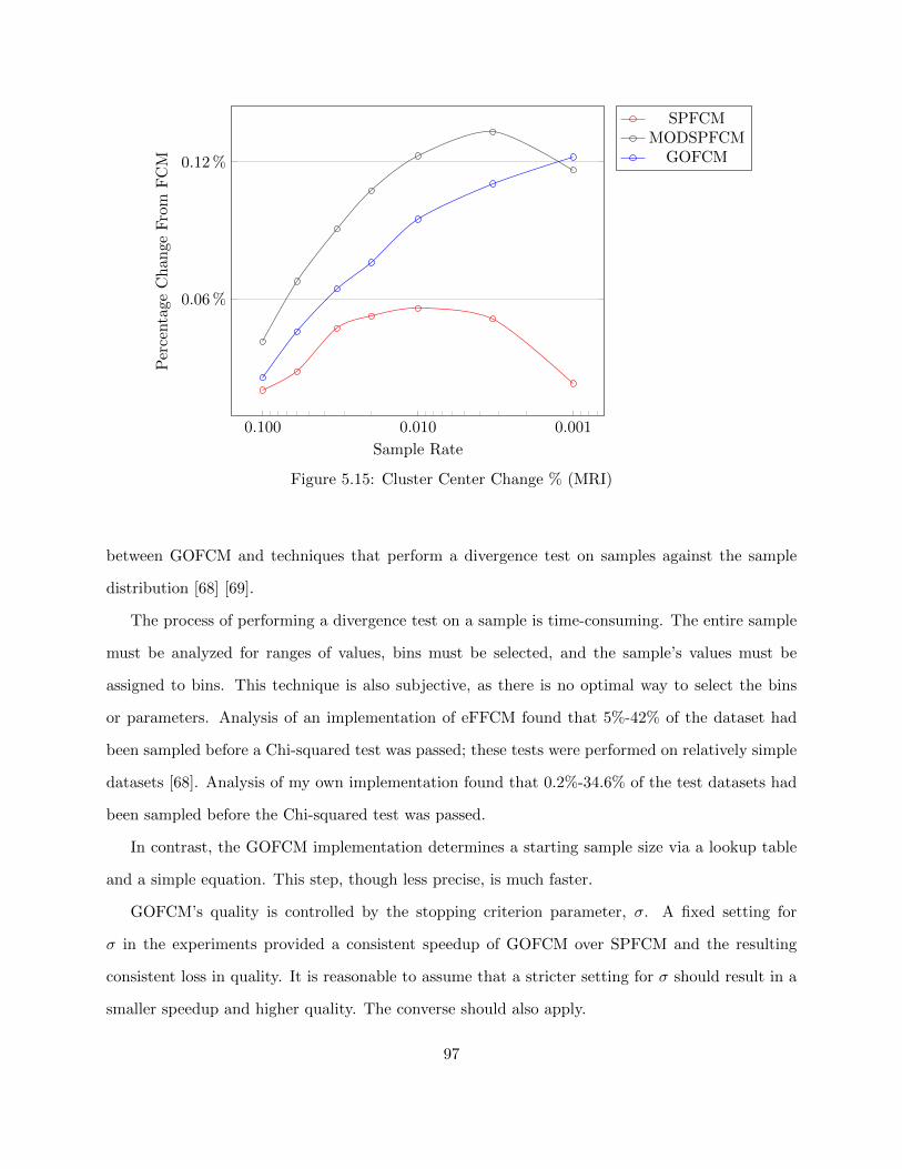
0.0010.0100.100
0.06 %
0.12 %
Sample Rate
Per
centa
geC
han
geF
rom
FC
M
SPFCMMODSPFCM
GOFCM
Figure 5.15: Cluster Center Change % (MRI)
between GOFCM and techniques that perform a divergence test on samples against the sample
distribution [68] [69].
The process of performing a divergence test on a sample is time-consuming. The entire sample
must be analyzed for ranges of values, bins must be selected, and the sample’s values must be
assigned to bins. This technique is also subjective, as there is no optimal way to select the bins
or parameters. Analysis of an implementation of eFFCM found that 5%-42% of the dataset had
been sampled before a Chi-squared test was passed; these tests were performed on relatively simple
datasets [68]. Analysis of my own implementation found that 0.2%-34.6% of the test datasets had
been sampled before the Chi-squared test was passed.
In contrast, the GOFCM implementation determines a starting sample size via a lookup table
and a simple equation. This step, though less precise, is much faster.
GOFCM’s quality is controlled by the stopping criterion parameter, σ. A fixed setting for
σ in the experiments provided a consistent speedup of GOFCM over SPFCM and the resulting
consistent loss in quality. It is reasonable to assume that a stricter setting for σ should result in a
smaller speedup and higher quality. The converse should also apply.
97
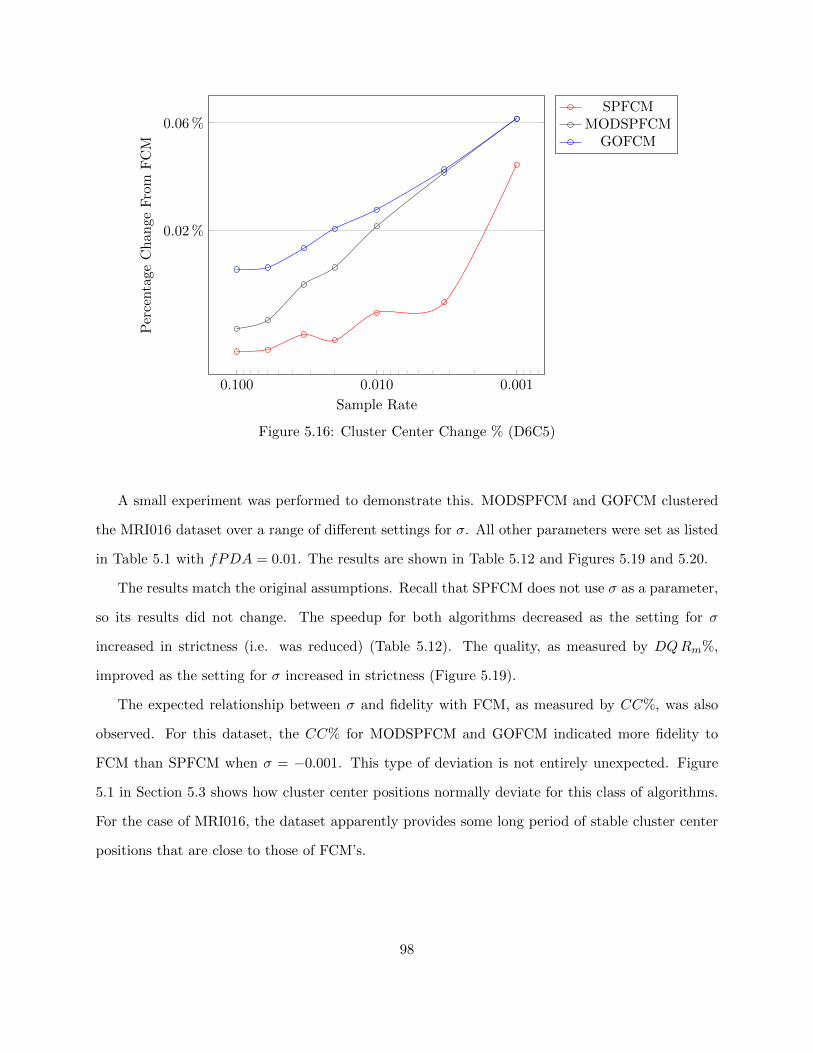
0.0010.0100.100
0.02 %
0.06 %
Sample Rate
Per
centa
geC
han
geF
rom
FC
M
SPFCMMODSPFCM
GOFCM
Figure 5.16: Cluster Center Change % (D6C5)
A small experiment was performed to demonstrate this. MODSPFCM and GOFCM clustered
the MRI016 dataset over a range of different settings for σ. All other parameters were set as listed
in Table 5.1 with fPDA = 0.01. The results are shown in Table 5.12 and Figures 5.19 and 5.20.
The results match the original assumptions. Recall that SPFCM does not use σ as a parameter,
so its results did not change. The speedup for both algorithms decreased as the setting for σ
increased in strictness (i.e. was reduced) (Table 5.12). The quality, as measured by DQRm%,
improved as the setting for σ increased in strictness (Figure 5.19).
The expected relationship between σ and fidelity with FCM, as measured by CC%, was also
observed. For this dataset, the CC% for MODSPFCM and GOFCM indicated more fidelity to
FCM than SPFCM when σ = −0.001. This type of deviation is not entirely unexpected. Figure
5.1 in Section 5.3 shows how cluster center positions normally deviate for this class of algorithms.
For the case of MRI016, the dataset apparently provides some long period of stable cluster center
positions that are close to those of FCM’s.
98
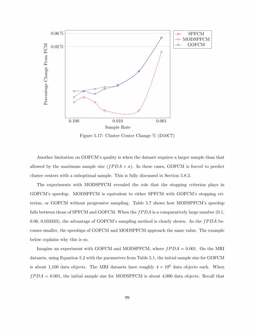
0.0010.0100.100
0.02 %
0.06 %
Sample Rate
Per
centa
geC
han
geF
rom
FC
M
SPFCMMODSPFCM
GOFCM
Figure 5.17: Cluster Center Change % (D10C7)
Another limitation on GOFCM’s quality is when the dataset requires a larger sample than that
allowed by the maximum sample size (fPDA × n). In these cases, GOFCM is forced to predict
cluster centers with a suboptimal sample. This is fully discussed in Section 5.8.2.
The experiments with MODSPFCM revealed the role that the stopping criterion plays in
GOFCM’s speedup. MODSPFCM is equivalent to either SPFCM with GOFCM’s stopping cri-
terion, or GOFCM without progressive sampling. Table 5.7 shows how MODSPFCM’s speedup
falls between those of SPFCM and GOFCM. When the fPDA is a comparatively large number (0.1,
0.06, 0.033333), the advantage of GOFCM’s sampling method is clearly shown. As the fPDA be-
comes smaller, the speedups of GOFCM and MODSPFCM approach the same value. The example
below explains why this is so.
Imagine an experiment with GOFCM and MODSPFCM, where fPDA = 0.001. On the MRI
datasets, using Equation 5.2 with the parameters from Table 5.1, the initial sample size for GOFCM
is about 1,100 data objects. The MRI datasets have roughly 4 × 10⁶ data objects each. When
fPDA = 0.001, the initial sample size for MODSPFCM is about 4,000 data objects. Recall that
99
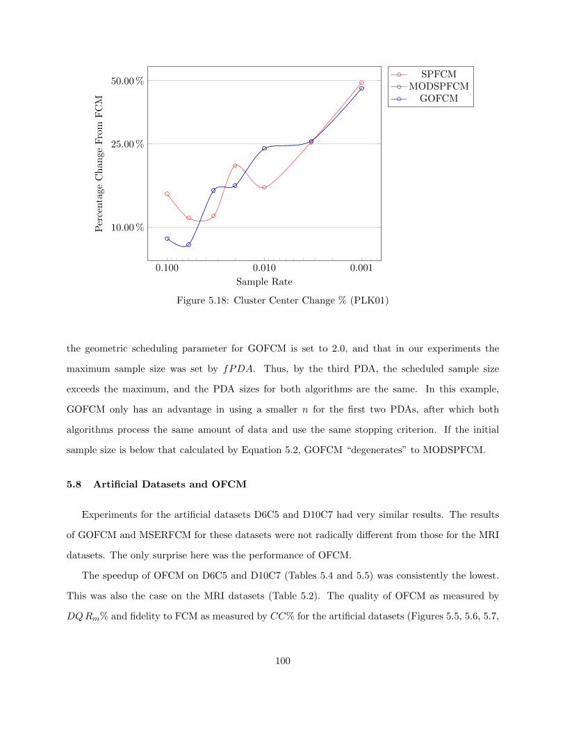
0.0010.0100.100
10.00 %
25.00 %
50.00 %
Sample Rate
Per
centa
geC
han
geF
rom
FC
M
SPFCMMODSPFCM
GOFCM
Figure 5.18: Cluster Center Change % (PLK01)
the geometric scheduling parameter for GOFCM is set to 2.0, and that in our experiments the
maximum sample size was set by fPDA. Thus, by the third PDA, the scheduled sample size
exceeds the maximum, and the PDA sizes for both algorithms are the same. In this example,
GOFCM only has an advantage in using a smaller n for the first two PDAs, after which both
algorithms process the same amount of data and use the same stopping criterion. If the initial
sample size is below that calculated by Equation 5.2, GOFCM “degenerates” to MODSPFCM.
5.8 Artificial Datasets and OFCM
Experiments for the artificial datasets D6C5 and D10C7 had very similar results. The results
of GOFCM and MSERFCM for these datasets were not radically different from those for the MRI
datasets. The only surprise here was the performance of OFCM.
The speedup of OFCM on D6C5 and D10C7 (Tables 5.4 and 5.5) was consistently the lowest.
This was also the case on the MRI datasets (Table 5.2). The quality of OFCM as measured by
DQRm% and fidelity to FCM as measured by CC% for the artificial datasets (Figures 5.5, 5.6, 5.7,
100
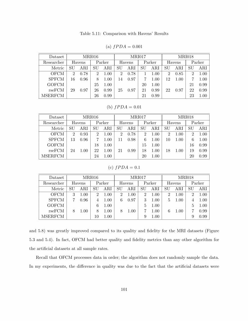
Table 5.11: Comparison with Havens’ Results
(a) fPDA = 0.001
Dataset MRI016 MRI017 MRI018
Researcher Havens Parker Havens Parker Havens Parker
Metric SU ARI SU ARI SU ARI SU ARI SU ARI SU ARI
OFCM 2 0.78 2 1.00 2 0.78 1 1.00 2 0.85 2 1.00SPFCM 16 0.96 8 1.00 14 0.97 7 1.00 12 1.00 7 1.00
GOFCM 25 1.00 20 1.00 21 0.99rseFCM 29 0.97 26 0.99 25 0.97 21 0.99 22 0.97 22 0.99
MSERFCM 26 0.99 21 0.99 23 1.00
(b) fPDA = 0.01
Dataset MRI016 MRI017 MRI018
Researcher Havens Parker Havens Parker Havens Parker
Metric SU ARI SU ARI SU ARI SU ARI SU ARI SU ARI
OFCM 2 0.93 2 1.00 2 0.78 2 1.00 2 1.00 2 1.00SPFCM 13 0.96 7 1.00 11 0.98 6 1.00 10 1.00 6 1.00
GOFCM 18 1.00 15 1.00 16 0.99rseFCM 24 1.00 22 1.00 21 0.99 18 1.00 18 1.00 19 0.99
MSERFCM 24 1.00 20 1.00 20 0.99
(c) fPDA = 0.1
Dataset MRI016 MRI017 MRI018
Researcher Havens Parker Havens Parker Havens Parker
Metric SU ARI SU ARI SU ARI SU ARI SU ARI SU ARI
OFCM 3 1.00 2 1.00 2 1.00 2 1.00 2 1.00 2 1.00SPFCM 7 0.96 4 1.00 6 0.97 3 1.00 5 1.00 4 1.00
GOFCM 6 1.00 5 1.00 5 1.00rseFCM 8 1.00 8 1.00 8 1.00 7 1.00 6 1.00 7 0.99
MSERFCM 10 1.00 9 1.00 9 0.99
and 5.8) was greatly improved compared to its quality and fidelity for the MRI datasets (Figure
5.3 and 5.4). In fact, OFCM had better quality and fidelity metrics than any other algorithm for
the artificial datasets at all sample rates.
Recall that OFCM processes data in order; the algorithm does not randomly sample the data.
In my experiments, the difference in quality was due to the fact that the artificial datasets were
101
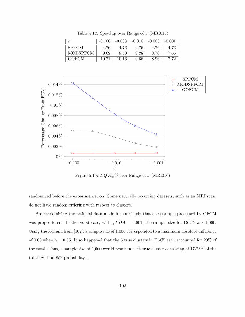
Table 5.12: Speedup over Range of σ (MRI016)
σ -0.100 -0.033 -0.010 -0.003 -0.001
SPFCM 4.76 4.76 4.76 4.76 4.76
MODSPFCM 9.62 9.50 9.28 8.70 7.66
GOFCM 10.71 10.16 9.66 8.96 7.72
−0.001−0.010−0.100
0 %
0.002 %
0.004 %
0.006 %
0.008 %
0.01 %
0.012 %
0.014 %
σ
Per
centa
geC
han
geF
rom
FC
M
SPFCMMODSPFCM
GOFCM
Figure 5.19: DQRm% over Range of σ (MRI016)
randomized before the experimentation. Some naturally occurring datasets, such as an MRI scan,
do not have random ordering with respect to clusters.
Pre-randomizing the artificial data made it more likely that each sample processed by OFCM
was proportional. In the worst case, with fPDA = 0.001, the sample size for D6C5 was 1,000.
Using the formula from [102], a sample size of 1,000 corresponded to a maximum absolute difference
of 0.03 when α = 0.05. It so happened that the 5 true clusters in D6C5 each accounted for 20% of
the total. Thus, a sample size of 1,000 would result in each true cluster consisting of 17-23% of the
total (with a 95% probability).
102
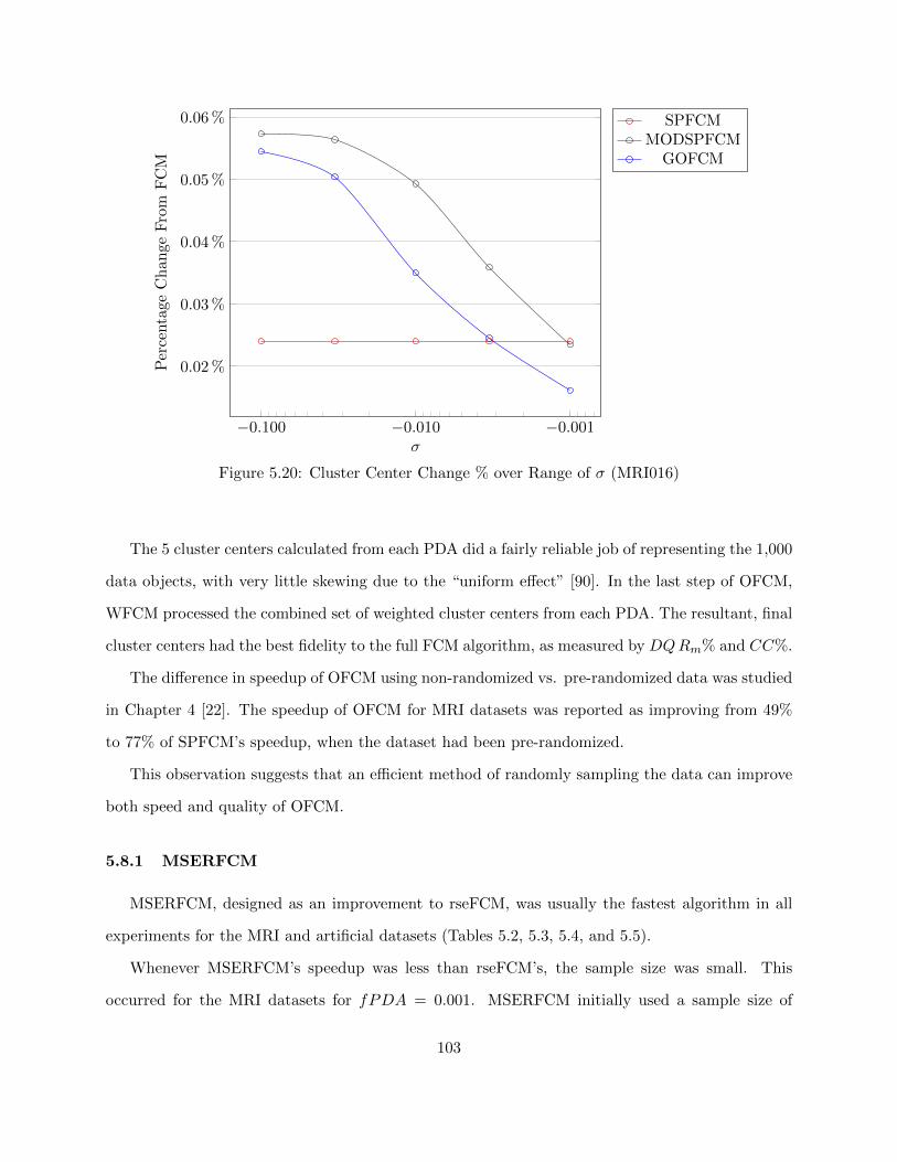
−0.001−0.010−0.100
0.02 %
0.03 %
0.04 %
0.05 %
0.06 %
σ
Per
centa
geC
han
geF
rom
FC
M
SPFCMMODSPFCM
GOFCM
Figure 5.20: Cluster Center Change % over Range of σ (MRI016)
The 5 cluster centers calculated from each PDA did a fairly reliable job of representing the 1,000
data objects, with very little skewing due to the “uniform effect” [90]. In the last step of OFCM,
WFCM processed the combined set of weighted cluster centers from each PDA. The resultant, final
cluster centers had the best fidelity to the full FCM algorithm, as measured by DQRm% and CC%.
The difference in speedup of OFCM using non-randomized vs. pre-randomized data was studied
in Chapter 4 [22]. The speedup of OFCM for MRI datasets was reported as improving from 49%
to 77% of SPFCM’s speedup, when the dataset had been pre-randomized.
This observation suggests that an efficient method of randomly sampling the data can improve
both speed and quality of OFCM.
5.8.1 MSERFCM
MSERFCM, designed as an improvement to rseFCM, was usually the fastest algorithm in all
experiments for the MRI and artificial datasets (Tables 5.2, 5.3, 5.4, and 5.5).
Whenever MSERFCM’s speedup was less than rseFCM’s, the sample size was small. This
occurred for the MRI datasets for fPDA = 0.001. MSERFCM initially used a sample size of
103
1,147 (Equation 5.2 with c=3) to calculate the starting cluster centers for FCM with a subsequent
sample size of about 4,000 objects. So, in these cases, MSERFCM processed over 5,000 objects,
while rseFCM processed about 4,000 objects. The speedup gained from a better set of starting
cluster centers was not enough to compensate for the time taken to process the increased amount
of data.
When D6C5 (n = 106) was clustered with the parameter fPDA = 0.001, the estimated sample
size to predict cluster centers was 3,184. In this case, the estimated sample size exceeded the user-
specified sample size (n × fPDA), and the MSERFCM algorithm degenerated to rseFCM with a
sample size of 3,184. This explains the faster performance of rseFCM, which used the user-specified
sample size of 1,000.
With respect to quality, MSERFCM was a better choice than rseFCM the majority of the time.
This is expected in situations where MSERFCM processed a larger sample size than rseFCM. In
the example above, MSERFCM processed a random sample three times larger, making it likely
that MSERFCM would have more fidelity to FCM.
The situation where the estimated sample size exceeded the user-specified sample size occurred
in 6 out of the 25 experiments using the MRI and artificial datasets. By design, MSERFCM
draws a separate sample to calculate the set of starting cluster centers to improve speedup. Both
MSERFCM and rseFCM use the same-size samples to cluster the dataset, so one would expect no
difference in quality between MSERFCM and rseFCM in the remaining 19 experiments.
This, however, was not the case. Of the remaining 12 MRI experiments, MSERFCM had
(ignoring ties) average quality and fidelity better than rseFCM’s: 67% of the time for the DQRm%
metric, and 72% of the time for the CC% metric. Of the remaining 7 artificial dataset experiments,
MSERFCM had (ignoring ties) average fidelity better than rseFCM’s: 67% of the time for both
the DQRm% and the CC% metrics.
FCM is guaranteed to converge to a local (or global) minimum or saddlepoint [91]. One pos-
sibility is that the calculated starting cluster centers for MSERFCM allow for better discovery of
local minima than do the randomly determined starting cluster centers for rseFCM. Research using
the HCM algorithm supports this observation. A comprehensive study of different initialization
104
methods for HCM, showed variation in quality by initialization method, as measured by final objec-
tive function value [108]. The runtime also varied by initialization method. Bradley and Fayyad’s
seminal paper on initialization methods also reported that a refined starting point for HCM could
improve runtime and quality [61]. Research using the FCM algorithm, discussed in Section 2.3.1,
also reports how an improved starting point for FCM improves runtime.
5.8.2 Plankton Dataset Challenges
Clustering the full plankton dataset, PLK01, showed the limitations and capabilities of the
algorithms.
The speedup for all algorithms on PLK01 (Table 5.6) is greater than the corresponding speedup
for the MRI datasets (Table 5.2) except MSERFCM. The MSERFCM algorithm has a consistent
but small speedup, just barely greater than that of OFCM.
This is so because of the sample size rules for MSERFCM. Thompson’s method (Equation 5.2)
estimates a minimum sample size of 50,944 for PLK01. Thus, in all experiments, MSERFCM
degenerates to rseFCM, with a sample size of 50,944. In contrast, the largest sample size for the
other algorithms is 20,328, when fPDA = 0.1.
Note that MSERFCM had the best quality (Figure 5.10). It was also the only one to have
consistent quality across all experiments, but this was to be expected, since the algorithm used the
same data samples in each experiment. MSERFCM’s CC% metric for PLK01 was 5.56%, and its
DQRm% was -0.0078%, suggesting that MSERFCM returned quality results superior to those of
FCM.
Statistical significance for the small difference in Rm between FCM and MSERFCM was tested
for, using a one-tailed Welch’s t-test. The t-test returned t = 0.43 with 50 d.f. This corresponds
to p = 0.3345, which is not considered statistically significant.
The eFFCM algorithm had fairly consistent, good-quality results on PLK01, but eFFCM has a
mechanism to increase its sample size dynamically if statistical measures are not met. The average
sample sizes of eFFCM for PLK01 ranged from 10.7% to 34.6%. All other algorithms suffered
a degradation of quality as the sample size was reduced. This was attributable to suboptimal
105

sample sizes. The fidelity to FCM, as measured by CC%, made these results unusable for many
applications of clustering.
The quality of the results from MSERFCM and eFFCM demonstrated the utility of using a
statistical method for determining sample size.
The PLK01 dataset also provided a nice demonstration of GOFCM’s operation. As with
MSERFCM, the estimated minimum sample size was greater than the user-defined sample size
(fPDA × n). What happened here was that GOFCM degenerated to use the same, consistent
sample rate as SPFCM.
When this occurred, the only difference between SPFCM and GOFCM was the stopping cri-
terion. SPFCM always processed 100% of the data, but GOFCM stopped short of that if the
stopping criterion were met. An examination of Table 5.6 shows that SPFCM and GOFCM had
a similar speedup when the fPDA (sample rate) was 0.1, and GOFCM’s speedup increased com-
pared to SPFCM’s as the fPDA decreased. Figure 5.9 shows that the DQRm% for both algorithms
increased as the fPDA decreased, with SPFCM’s DQRm% consistently lower than GOFCM’s.
Observe the CC% of SPFCM, OFCM, and GOFCM when the fPDA = 0.001 (Figure 5.10).
Note that the values are very similar. When fPDA = 0.001, the sample size is only 204. Exper-
imentation was kept consistent across all datasets; in reality there is no reason for such a small
sample. Recall that c = 20 for PLK01. The cluster representation for PLK01 is not uniform, and
the sample size is small, making it unlikely that all clusters are even represented in each sample.
The base FCM algorithm will still try to fit 20 clusters, likely resulting in predicted cluster centers
unrepresentative of the full dataset.
106
Chapter 6: Accelerating FCMdd
“It’s not too far, it just seems like it is.” - Lawrence “Yogi” Berra [2]
6.1 Distributed FCMdd
Breaking a dataset into overlapping or disjoint subsets and then performing clustering is not a
new idea. Strehl and Ghosh provided an analysis of how best to combine clustering results from
different subsets of data [109]. Their work focused on solving the problem of efficiently aligning
like clusters, rather than accelerating a clustering algorithm, but they do mention that speedups
can occur.
Hore based his algorithms, SPFCM and OFCM, on clustering subsets of the full dataset and on
combining the results from disjoint sets [46] [65] [71]. Labroche duplicated Hore’s algorithms for
use with relational data, substituting FCMdd for FCM [54].
The Distributed FCMdd (DFCMdd), as the name implies, is an accelerated algorithm that
distributes a relational dataset into disjoint subsets. It is designed to speedup the clustering by
both reducing the sample size and by decreasing the average number of iterations. Quality is
preserved by exploiting the observations about OFCM’s performance on pre-randomized data.
The DFCMdd algorithm has two stages. In stage one, it breaks the dataset into a user-defined
number of subsets, called folds. Each data object in the dataset is randomly assigned into one of
f folds. The folds are equal in size, so for a dataset with n objects, each fold has nf data objects.
Each fold is then clustered using FCMdd (also referred to in this chapter as the reference
algorithm) to return a set of c medoids. After all folds have been clustered, a set of f × c medoids
are retained. This dataset is called the “medoid dataset.”
107

In stage two, a “linking method” is used to cluster the medoid dataset. The linking method
produces a set of c medoids as a final clustering solution.
6.1.1 Linking Methods
The linking method combines the results from each fold into one solution. This is a concept
similar to a “consensus function” in cluster ensembles [109], except for the fact that DFCMdd
assumes that the data in each fold is disjoint and that the strength of the relation between any two
data objects is known.
Four different linking methods were developed. The first linking method (LM1) reapplies
FCMdd to the medoid dataset. The initial medoids used by FCMdd are randomly selected. This
arrangement is nearly identical to OFCMD [54], except in that the medoid dataset is not weighted.
One necessary decision was whether or not to weight the medoids and to use a weighted version
of FCMdd, which is similar to work by LaBroche [54] or Mei [110]. A consideration was that two
of the linking methods use Single Linkage and weights are not meaningful to that algorithm. Thus,
a weighting strategy was not implemented.
The second linking method (LM2) applies Single Linkage to the medoid dataset. As described
in Section 2.1.1, the last c − 1 links are removed to separate the final dendrogram into c clusters.
Medoids from each cluster are defined as the data object that has the smallest total dissimilarity
over all objects in its cluster. The medoid, for a cluster k, is calculated by:
q = argmin1≤j≤n;xj∈Xk
n∑i=1
ρ(xi, xj); vk = xq; (6.1)
where:
X is a dataset where n = |X|, and Xk is the subset assigned to the kth cluster.
xi is the ith data object.
V is the set of cluster centers; vk is the kth cluster center.
ρ(xi, xj) is the dissimilarity between the ith and jth data objects.
108
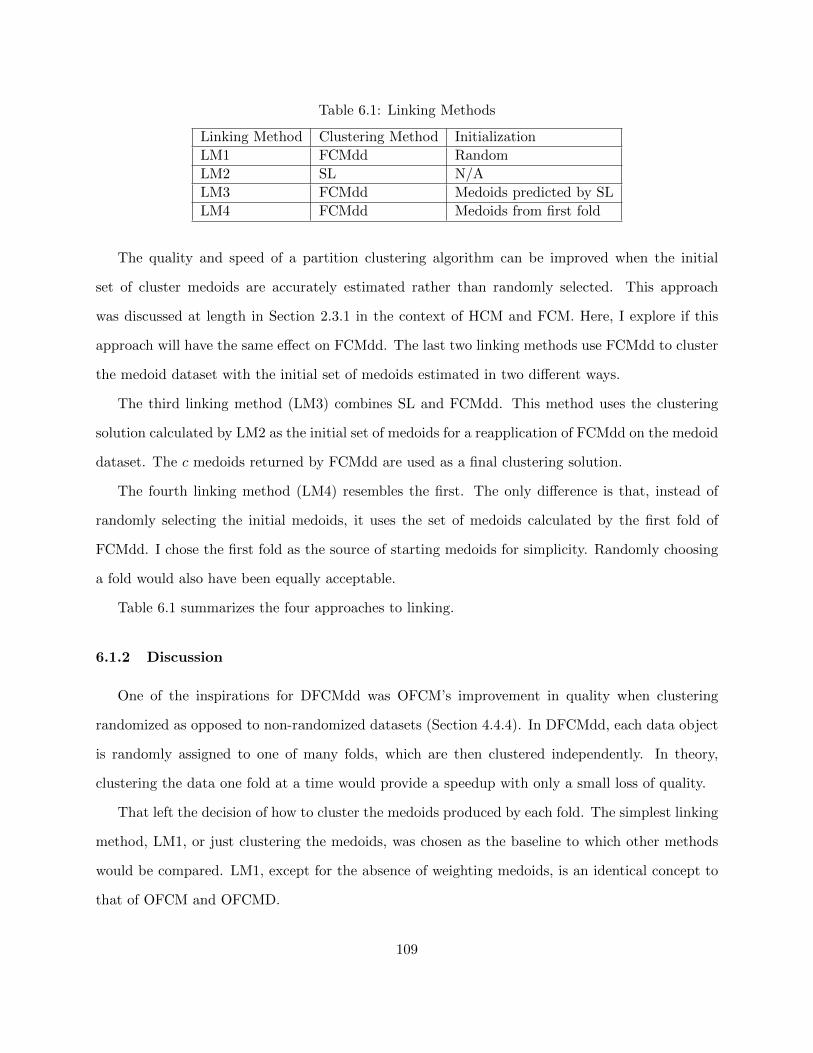
Table 6.1: Linking Methods
Linking Method Clustering Method Initialization
LM1 FCMdd Random
LM2 SL N/A
LM3 FCMdd Medoids predicted by SL
LM4 FCMdd Medoids from first fold
The quality and speed of a partition clustering algorithm can be improved when the initial
set of cluster medoids are accurately estimated rather than randomly selected. This approach
was discussed at length in Section 2.3.1 in the context of HCM and FCM. Here, I explore if this
approach will have the same effect on FCMdd. The last two linking methods use FCMdd to cluster
the medoid dataset with the initial set of medoids estimated in two different ways.
The third linking method (LM3) combines SL and FCMdd. This method uses the clustering
solution calculated by LM2 as the initial set of medoids for a reapplication of FCMdd on the medoid
dataset. The c medoids returned by FCMdd are used as a final clustering solution.
The fourth linking method (LM4) resembles the first. The only difference is that, instead of
randomly selecting the initial medoids, it uses the set of medoids calculated by the first fold of
FCMdd. I chose the first fold as the source of starting medoids for simplicity. Randomly choosing
a fold would also have been equally acceptable.
Table 6.1 summarizes the four approaches to linking.
6.1.2 Discussion
One of the inspirations for DFCMdd was OFCM’s improvement in quality when clustering
randomized as opposed to non-randomized datasets (Section 4.4.4). In DFCMdd, each data object
is randomly assigned to one of many folds, which are then clustered independently. In theory,
clustering the data one fold at a time would provide a speedup with only a small loss of quality.
That left the decision of how to cluster the medoids produced by each fold. The simplest linking
method, LM1, or just clustering the medoids, was chosen as the baseline to which other methods
would be compared. LM1, except for the absence of weighting medoids, is an identical concept to
that of OFCM and OFCMD.
109
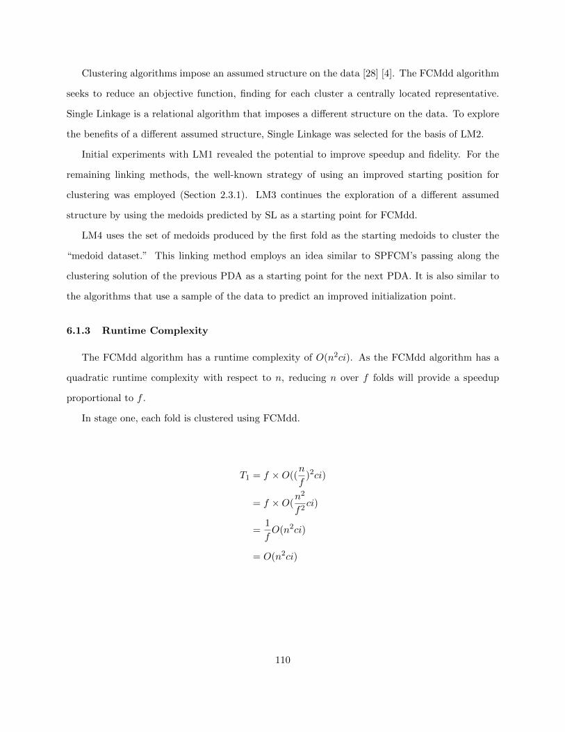
Clustering algorithms impose an assumed structure on the data [28] [4]. The FCMdd algorithm
seeks to reduce an objective function, finding for each cluster a centrally located representative.
Single Linkage is a relational algorithm that imposes a different structure on the data. To explore
the benefits of a different assumed structure, Single Linkage was selected for the basis of LM2.
Initial experiments with LM1 revealed the potential to improve speedup and fidelity. For the
remaining linking methods, the well-known strategy of using an improved starting position for
clustering was employed (Section 2.3.1). LM3 continues the exploration of a different assumed
structure by using the medoids predicted by SL as a starting point for FCMdd.
LM4 uses the set of medoids produced by the first fold as the starting medoids to cluster the
“medoid dataset.” This linking method employs an idea similar to SPFCM’s passing along the
clustering solution of the previous PDA as a starting point for the next PDA. It is also similar to
the algorithms that use a sample of the data to predict an improved initialization point.
6.1.3 Runtime Complexity
The FCMdd algorithm has a runtime complexity of O(n2ci). As the FCMdd algorithm has a
quadratic runtime complexity with respect to n, reducing n over f folds will provide a speedup
proportional to f .
In stage one, each fold is clustered using FCMdd.
T1 = f ×O((n
f)2ci)
= f ×O(n2
f2ci)
=1
fO(n2ci)
= O(n2ci)
110
The value 1f is a constant and is not considered as part of the runtime complexity. For practical
purposes, it should produce a speedup roughly f times the reference algorithm.
One must also consider the time taken by the linking method in stage two. Both SL and FCMdd
have a quadratic runtime complexity with respect to n. In this case, though, the number of data
objects equals f×c. If one assumes that fc << n, the amount of time taken by the linking method
is negligible.
6.2 Experiments
FCMdd and DFCMdd were compared in terms of speedup and quality on five real-world and
four artificial datasets: the real-world datasets were MRI016R, MRI017R, MRI018R, PLK02, and
Pendigits; the artificial datasets were D3C6-1, D3C6-2, D4C5, and D7C10. See Chapter 3 for
dataset details.
I performed additional preprocessing for the MRI datasets. There were 12,000 data objects
randomly selected from each original MRI dataset to serve as experimental datasets. The data
features were linearly scaled to fall in the range [0-1], based on the maximum and minimum values
in the original dataset.
The dataset sizes were kept relatively small compared to the experimentation using FCM and
its variants. FCMdd has a runtime complexity that is quadratic with respect to the number of data
objects. The size of datasets were balanced to ensure that enough data was present for a realistic
test, but small enough so that experimentation could be completed in a timely fashion.
The number of data objects was set to 12,000 in order to ensure that the sample proportionally
represented each class. As in Equation 5.2, Thompson’s formula estimates that a minimum sample
size of 1,178 is required in order to ensure a proportional sample when r = 0.10 at the 95%
confidence level given that c = 3. When one of the MRI datasets is broken into 10 folds, each fold
will have a proportional sample.
To verify that selection of 12,000 data objects was not merely an anomaly resulting in good
(or bad) performance, I created an additional MRI dataset containing 20,000 data objects. This
111
dataset, MRI017R-2, was created from MRI017 and was processed in a manner otherwise identical
to the other MRI datasets.
The artificial datasets consisted of either 12,000 or 16,000 data objects. Each data feature was
scaled so that the values fell in the range [0− 1].
6.2.1 Experimental Procedures
The FCMdd and Single Linkage algorithms are designed to cluster relational data. The data
objects in the datasets used for experimentation are vectors of numeric features. The numeric data
was converted to relational data by defining the dissimilarity function, ρ(xi, xj), as the Euclidean
distance.
All experiments consisted of 30 trials. Each dataset was clustered by the reference algorithm
(FCMdd). DFCMdd was used to cluster each dataset twice, once using 5 folds and the other
time using 10 folds. Each DFCMdd experiment resulted in a “medoid dataset” that contained the
medoids from each fold. Each of the four linking methods was applied to each medoid dataset.
Thus, there were four final sets of medoids from each experiment.
The runtime for each algorithm was recorded as the number of clock ticks that elapsed while
the algorithm was executing. Time taken to pre-process the data was not included in this time.
Equation 2.11 and the final set of medoids for each trial were used to calculate the cluster
membership for each data object. This calculated cluster membership was in turn used to calculate
Jm for each trial.
The intra CC% was calculated for each experiment. The inter CC% was calculated between the
reference algorithm clustering solution and each DFCMdd experiment that used the same dataset.
Before calculating CC%, cluster membership was “hardened,” i.e., each data object was assigned
solely to the cluster for which it had the highest membership. Details on intra and inter CC% are
in Section 2.4.3.
Accuracy was calculated for datasets for which the class identities were known.
112
6.2.2 Parameters
A few parameters needed to be set for FCMdd and DFCMdd. The number of clusters, c, was
set to the number of known classes in each dataset. Experiments were run for f = 5 and f = 10
folds. The fuzzifier, m, was set to 1.5 for all experiments. This is a lower setting than in my FCM
experiments, but Krishnapuram advises setting m at 1.5 or lower for FCMdd.
This is because m controls how fuzzy each cluster will be. The cluster centers, however, are
medoids and have a fuzzy membership in their cluster equal to one. Because m is an exponent,
it has no effect on the medoid’s fuzzy membership. However, a high setting of m will make the
fuzzy cluster memberships of all other data objects less distinct. This makes it less likely that the
medoid for each cluster will change [52].
The Single Linkage algorithm is deterministic and only requires the parameter c.
6.2.3 Results
The results for 10 datasets, 2 fold settings, and 4 linking methods created a large volume of
data. Complete results are available in Tables B.1 and B.2 in Appendix B. Representative subsets
of the results are presented here.
DFCMdd provides a speedup of about 6.5 times when there are 5 folds, and a speedup of about
14 times when there are 10 folds, regardless of linking method.
No linking method was consistently the fastest in all datasets. For the 20 experiments with
different combinations of datasets and fold settings, LM2 was fastest over seven experiments. For
any particular dataset and fold setting, the linking methods’ speedups did not differ much.
Table 6.2 illustrates the lack of variation in speedup of MRI016R, and Table 6.3 lists the average
speedup and standard deviation for each fold setting and linking method.
There was some variation in speedup across datasets, suggesting that some datasets were “eas-
ier” for DFCMdd to cluster than others. The speedup on dataset D3C6-1 was much higher than
those of the other datasets. If D3C6-1’s values are omitted, the speedup values in Table 6.3 fall
slightly, and the standard deviation is tightened. This is shown in Table 6.4.
113
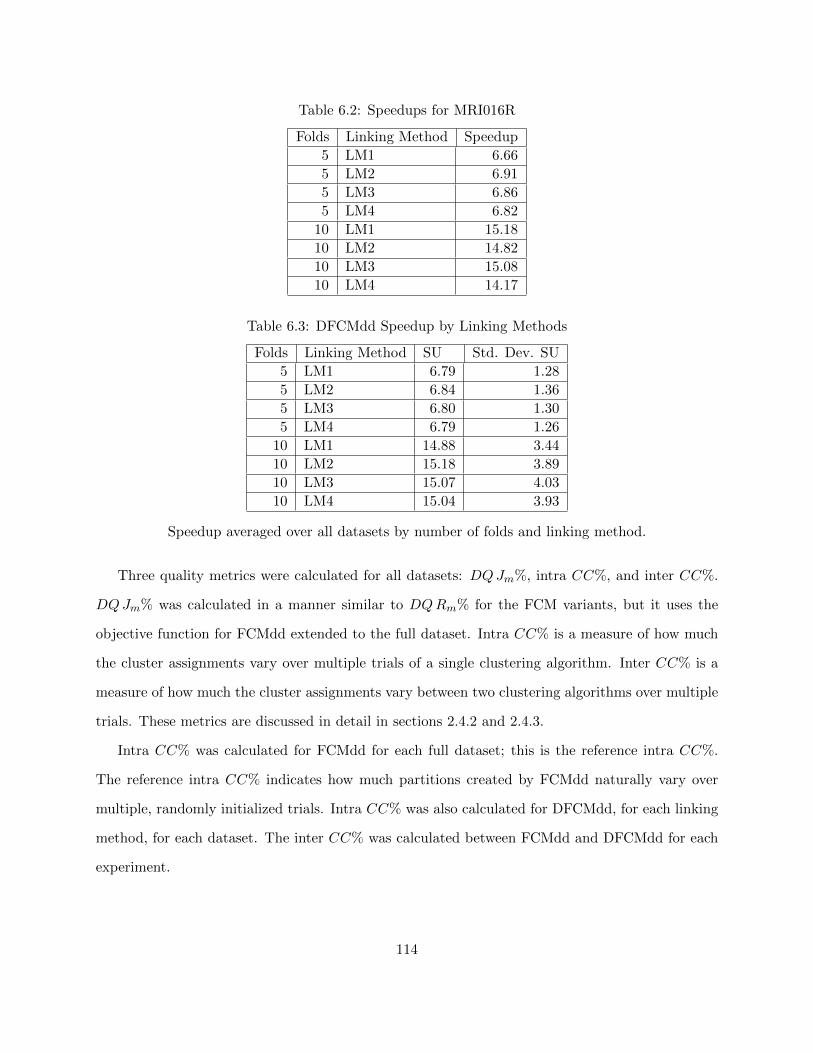
Table 6.2: Speedups for MRI016R
Folds Linking Method Speedup
5 LM1 6.66
5 LM2 6.91
5 LM3 6.86
5 LM4 6.82
10 LM1 15.18
10 LM2 14.82
10 LM3 15.08
10 LM4 14.17
Table 6.3: DFCMdd Speedup by Linking Methods
Folds Linking Method SU Std. Dev. SU
5 LM1 6.79 1.28
5 LM2 6.84 1.36
5 LM3 6.80 1.30
5 LM4 6.79 1.26
10 LM1 14.88 3.44
10 LM2 15.18 3.89
10 LM3 15.07 4.03
10 LM4 15.04 3.93
Speedup averaged over all datasets by number of folds and linking method.
Three quality metrics were calculated for all datasets: DQJm%, intra CC%, and inter CC%.
DQJm% was calculated in a manner similar to DQRm% for the FCM variants, but it uses the
objective function for FCMdd extended to the full dataset. Intra CC% is a measure of how much
the cluster assignments vary over multiple trials of a single clustering algorithm. Inter CC% is a
measure of how much the cluster assignments vary between two clustering algorithms over multiple
trials. These metrics are discussed in detail in sections 2.4.2 and 2.4.3.
Intra CC% was calculated for FCMdd for each full dataset; this is the reference intra CC%.
The reference intra CC% indicates how much partitions created by FCMdd naturally vary over
multiple, randomly initialized trials. Intra CC% was also calculated for DFCMdd, for each linking
method, for each dataset. The inter CC% was calculated between FCMdd and DFCMdd for each
experiment.
114
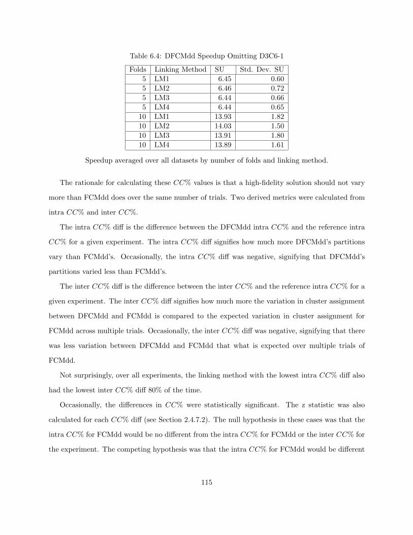
Table 6.4: DFCMdd Speedup Omitting D3C6-1
Folds Linking Method SU Std. Dev. SU
5 LM1 6.45 0.60
5 LM2 6.46 0.72
5 LM3 6.44 0.66
5 LM4 6.44 0.65
10 LM1 13.93 1.82
10 LM2 14.03 1.50
10 LM3 13.91 1.80
10 LM4 13.89 1.61
Speedup averaged over all datasets by number of folds and linking method.
The rationale for calculating these CC% values is that a high-fidelity solution should not vary
more than FCMdd does over the same number of trials. Two derived metrics were calculated from
intra CC% and inter CC%.
The intra CC% diff is the difference between the DFCMdd intra CC% and the reference intra
CC% for a given experiment. The intra CC% diff signifies how much more DFCMdd’s partitions
vary than FCMdd’s. Occasionally, the intra CC% diff was negative, signifying that DFCMdd’s
partitions varied less than FCMdd’s.
The inter CC% diff is the difference between the inter CC% and the reference intra CC% for a
given experiment. The inter CC% diff signifies how much more the variation in cluster assignment
between DFCMdd and FCMdd is compared to the expected variation in cluster assignment for
FCMdd across multiple trials. Occasionally, the inter CC% diff was negative, signifying that there
was less variation between DFCMdd and FCMdd that what is expected over multiple trials of
FCMdd.
Not surprisingly, over all experiments, the linking method with the lowest intra CC% diff also
had the lowest inter CC% diff 80% of the time.
Occasionally, the differences in CC% were statistically significant. The z statistic was also
calculated for each CC% diff (see Section 2.4.7.2). The null hypothesis in these cases was that the
intra CC% for FCMdd would be no different from the intra CC% for FCMdd or the inter CC% for
the experiment. The competing hypothesis was that the intra CC% for FCMdd would be different
115
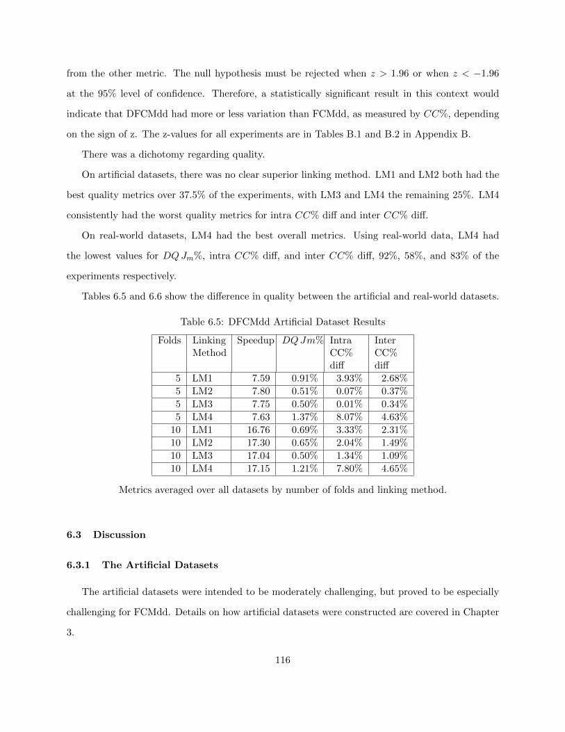
from the other metric. The null hypothesis must be rejected when z > 1.96 or when z < −1.96
at the 95% level of confidence. Therefore, a statistically significant result in this context would
indicate that DFCMdd had more or less variation than FCMdd, as measured by CC%, depending
on the sign of z. The z-values for all experiments are in Tables B.1 and B.2 in Appendix B.
There was a dichotomy regarding quality.
On artificial datasets, there was no clear superior linking method. LM1 and LM2 both had the
best quality metrics over 37.5% of the experiments, with LM3 and LM4 the remaining 25%. LM4
consistently had the worst quality metrics for intra CC% diff and inter CC% diff.
On real-world datasets, LM4 had the best overall metrics. Using real-world data, LM4 had
the lowest values for DQJm%, intra CC% diff, and inter CC% diff, 92%, 58%, and 83% of the
experiments respectively.
Tables 6.5 and 6.6 show the difference in quality between the artificial and real-world datasets.
Table 6.5: DFCMdd Artificial Dataset Results
Folds LinkingMethod
Speedup DQJm% IntraCC%diff
InterCC%diff
5 LM1 7.59 0.91% 3.93% 2.68%
5 LM2 7.80 0.51% 0.07% 0.37%
5 LM3 7.75 0.50% 0.01% 0.34%
5 LM4 7.63 1.37% 8.07% 4.63%
10 LM1 16.76 0.69% 3.33% 2.31%
10 LM2 17.30 0.65% 2.04% 1.49%
10 LM3 17.04 0.50% 1.34% 1.09%
10 LM4 17.15 1.21% 7.80% 4.65%
Metrics averaged over all datasets by number of folds and linking method.
6.3 Discussion
6.3.1 The Artificial Datasets
The artificial datasets were intended to be moderately challenging, but proved to be especially
challenging for FCMdd. Details on how artificial datasets were constructed are covered in Chapter
3.
116
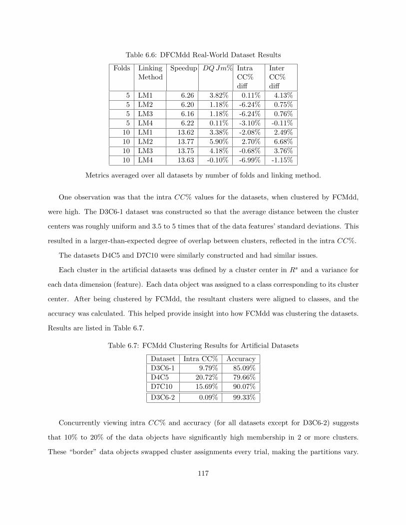
Table 6.6: DFCMdd Real-World Dataset Results
Folds LinkingMethod
Speedup DQJm% IntraCC%diff
InterCC%diff
5 LM1 6.26 3.82% 0.11% 4.13%
5 LM2 6.20 1.18% -6.24% 0.75%
5 LM3 6.16 1.18% -6.24% 0.76%
5 LM4 6.22 0.11% -3.10% -0.11%
10 LM1 13.62 3.38% -2.08% 2.49%
10 LM2 13.77 5.90% 2.70% 6.68%
10 LM3 13.75 4.18% -0.68% 3.76%
10 LM4 13.63 -0.10% -6.99% -1.15%
Metrics averaged over all datasets by number of folds and linking method.
One observation was that the intra CC% values for the datasets, when clustered by FCMdd,
were high. The D3C6-1 dataset was constructed so that the average distance between the cluster
centers was roughly uniform and 3.5 to 5 times that of the data features’ standard deviations. This
resulted in a larger-than-expected degree of overlap between clusters, reflected in the intra CC%.
The datasets D4C5 and D7C10 were similarly constructed and had similar issues.
Each cluster in the artificial datasets was defined by a cluster center in Rs and a variance for
each data dimension (feature). Each data object was assigned to a class corresponding to its cluster
center. After being clustered by FCMdd, the resultant clusters were aligned to classes, and the
accuracy was calculated. This helped provide insight into how FCMdd was clustering the datasets.
Results are listed in Table 6.7.
Table 6.7: FCMdd Clustering Results for Artificial Datasets
Dataset Intra CC% Accuracy
D3C6-1 9.79% 85.09%
D4C5 20.72% 79.66%
D7C10 15.69% 90.07%
D3C6-2 0.09% 99.33%
Concurrently viewing intra CC% and accuracy (for all datasets except for D3C6-2) suggests
that 10% to 20% of the data objects have significantly high membership in 2 or more clusters.
These “border” data objects swapped cluster assignments every trial, making the partitions vary.
117
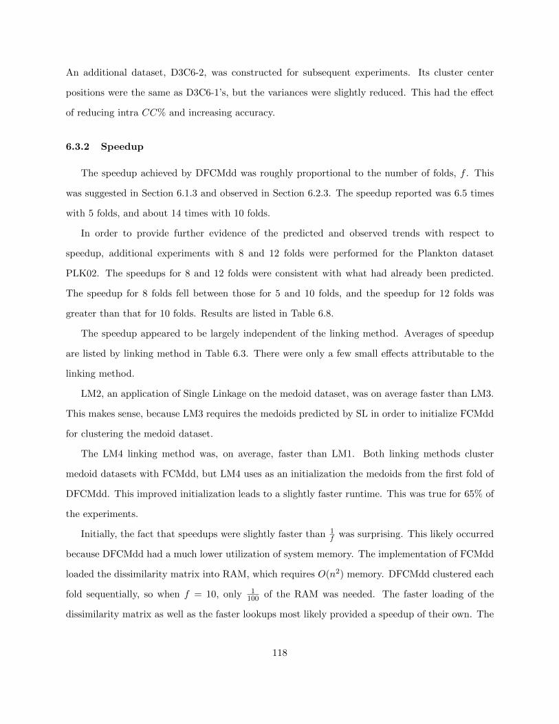
An additional dataset, D3C6-2, was constructed for subsequent experiments. Its cluster center
positions were the same as D3C6-1’s, but the variances were slightly reduced. This had the effect
of reducing intra CC% and increasing accuracy.
6.3.2 Speedup
The speedup achieved by DFCMdd was roughly proportional to the number of folds, f . This
was suggested in Section 6.1.3 and observed in Section 6.2.3. The speedup reported was 6.5 times
with 5 folds, and about 14 times with 10 folds.
In order to provide further evidence of the predicted and observed trends with respect to
speedup, additional experiments with 8 and 12 folds were performed for the Plankton dataset
PLK02. The speedups for 8 and 12 folds were consistent with what had already been predicted.
The speedup for 8 folds fell between those for 5 and 10 folds, and the speedup for 12 folds was
greater than that for 10 folds. Results are listed in Table 6.8.
The speedup appeared to be largely independent of the linking method. Averages of speedup
are listed by linking method in Table 6.3. There were only a few small effects attributable to the
linking method.
LM2, an application of Single Linkage on the medoid dataset, was on average faster than LM3.
This makes sense, because LM3 requires the medoids predicted by SL in order to initialize FCMdd
for clustering the medoid dataset.
The LM4 linking method was, on average, faster than LM1. Both linking methods cluster
medoid datasets with FCMdd, but LM4 uses as an initialization the medoids from the first fold of
DFCMdd. This improved initialization leads to a slightly faster runtime. This was true for 65% of
the experiments.
Initially, the fact that speedups were slightly faster than 1f was surprising. This likely occurred
because DFCMdd had a much lower utilization of system memory. The implementation of FCMdd
loaded the dissimilarity matrix into RAM, which requires O(n2) memory. DFCMdd clustered each
fold sequentially, so when f = 10, only 1100 of the RAM was needed. The faster loading of the
dissimilarity matrix as well as the faster lookups most likely provided a speedup of their own. The
118
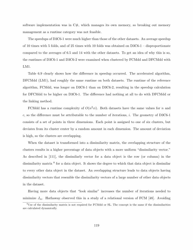
software implementation was in C#, which manages its own memory, so breaking out memory
management as a runtime category was not feasible.
The speedups of D3C6-1 were much higher than those of the other datasets. An average speedup
of 10 times with 5 folds, and of 25 times with 10 folds was obtained on D3C6-1 – disproportionate
compared to the averages of 6.5 and 14 with the other datasets. To get an idea of why this is so,
the runtimes of D3C6-1 and D3C6-2 were examined when clustered by FCMdd and DFCMdd with
LM1.
Table 6.9 clearly shows how the difference in speedup occurred. The accelerated algorithm,
DFCMdd (LM1), had roughly the same runtime on both datasets. The runtime of the reference
algorithm, FCMdd, was longer on D3C6-1 than on D3C6-2, resulting in the speedup calculation
for DFCMdd to be higher on D3C6-1. The difference had nothing at all to do with DFCMdd or
the linking method.
FCMdd has a runtime complexity of O(n2ci). Both datasets have the same values for n and
c, so the difference must be attributable to the number of iterations, i. The geometry of D3C6-1
consists of a set of points in three dimensions. Each point is assigned to one of six clusters, but
deviates from its cluster center by a random amount in each dimension. The amount of deviation
is high, so the clusters are overlapping.
When the dataset is transformed into a dissimilarity matrix, the overlapping structure of the
clusters results in a higher percentage of data objects with a more uniform “dissimilarity vector.”
As described in [111], the dissimilarly vector for a data object is the row (or column) in the
dissimilarity matrix 8 for a data object. It shows the degree to which that data object is dissimilar
to every other data object in the dataset. An overlapping structure leads to data objects having
dissimilarity vectors that resemble the dissimilarity vectors of a large number of other data objects
in the dataset.
Having more data objects that “look similar” increases the number of iterations needed to
minimize Jm. Hathaway observed this in a study of a relational version of FCM [48]. Avoiding
8Use of the dissimilarity matrix is not required for FCMdd or SL. The concept is the same if the dissimilaritiesare calculated dynamically.
119
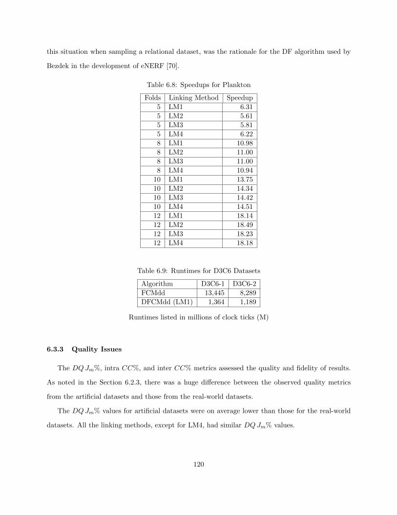
this situation when sampling a relational dataset, was the rationale for the DF algorithm used by
Bezdek in the development of eNERF [70].
Table 6.8: Speedups for Plankton
Folds Linking Method Speedup
5 LM1 6.31
5 LM2 5.61
5 LM3 5.81
5 LM4 6.22
8 LM1 10.98
8 LM2 11.00
8 LM3 11.00
8 LM4 10.94
10 LM1 13.75
10 LM2 14.34
10 LM3 14.42
10 LM4 14.51
12 LM1 18.14
12 LM2 18.49
12 LM3 18.23
12 LM4 18.18
Table 6.9: Runtimes for D3C6 Datasets
Algorithm D3C6-1 D3C6-2
FCMdd 13,445 8,289
DFCMdd (LM1) 1,364 1,189
Runtimes listed in millions of clock ticks (M)
6.3.3 Quality Issues
The DQJm%, intra CC%, and inter CC% metrics assessed the quality and fidelity of results.
As noted in the Section 6.2.3, there was a huge difference between the observed quality metrics
from the artificial datasets and those from the real-world datasets.
The DQJm% values for artificial datasets were on average lower than those for the real-world
datasets. All the linking methods, except for LM4, had similar DQJm% values.
120
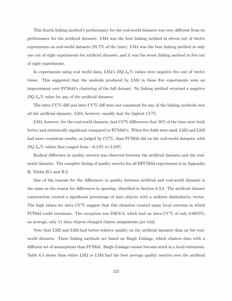
This fourth linking method’s performance for the real-world datasets was very different from its
performance for the artificial datasets. LM4 was the best linking method in eleven out of twelve
experiments on real-world datasets (91.7% of the time). LM4 was the best linking method in only
one out of eight experiments for artificial datasets, and it was the worst linking method in five out
of eight experiments.
In experiments using real world data, LM4’s DQJm% values were negative five out of twelve
times. This suggested that the medoids produced by LM4 in these five experiments were an
improvement over FCMdd’s clustering of the full dataset. No linking method returned a negative
DQJm% value for any of the artificial datasets.
The intra CC% diff and inter CC% diff were not consistent for any of the linking methods over
all the artificial datasets. LM4, however, usually had the highest CC%.
LM4, however, for the real-world datasets, had CC% differences that 58% of the time were both
better and statistically significant compared to FCMdd’s. When five folds were used, LM2 and LM3
had more consistent results, as judged by CC%, than FCMdd did on the real-world datasets, with
DQJm% values that ranged from −0.14% to 3.24%.
Radical difference in quality metrics was observed between the artificial datasets and the real-
world datasets. The complete listing of quality metrics for all DFCMdd experiments is in Appendix
B, Tables B.1 and B.2.
One of the reasons for the differences in quality between artificial and real-world datasets is
the same as the reason for differences in speedup, identified in Section 6.3.2. The artificial dataset
construction created a significant percentage of data objects with a uniform dissimilarity vector.
The high values for intra CC% suggest that this situation created many local extrema in which
FCMdd could terminate. The exception was D3C6-2, which had an intra CC% of only 0.0915%;
on average, only 11 data objects changed cluster assignments per trial.
Note that LM2 and LM3 had better relative quality on the artificial datasets than on the real-
world datasets. These linking methods are based on Single Linkage, which clusters data with a
different set of assumptions than FCMdd. Single Linkage cannot become stuck in a local extremum.
Table 6.5 shows than either LM2 or LM3 had the best average quality metrics over the artificial
121
datasets. For many experiments, LM2 and LM3 returned identical quality results. This meant that
the medoids produced by Single Linkage, when used as an initialization for FCMdd, were already
in a local extremum and did not deviate further.
The difference between LM1 and LM4 on the artificial datasets was surprising. The intent of
LM4 was to use an initial set of medoids based on a sample (the first fold) to produce higher-quality
results. Unfortunately, LM4 had clearly inferior quality results compared to LM1 for the artificial
datasets. This difference in quality between LM1 and LM4 for the artificial datasets needed further
investigation.
Diagnostic logs and raw results for D3C6-1’s 30-trial experiments were carefully analyzed. In
20% of the trials, the final sets of medoids from LM1 and LM4 were identical. In the rest, the final
set of medoids from LM4 usually had worse quality than that from LM1. Recall that LM4 uses the
medoids from the first fold as an initialization to cluster the medoid dataset. In a few of the trials,
the final set of medoids did not deviate from the initialization set. This is because the medoids
from the first fold were therefore already in a local extremum of the medoid dataset. In many of
the other trials, the final set of medoids only deviated from the initial set of medoids by one or two
of the medoids. Thus, the medoids from the first fold were already very close to a local extremum.
In many of these cases, the initial set of medoids were at or near a local extremum that had an
inferior (high) objective function value.
The real-world datasets had markedly different quality results from the artificial datasets. As the
algorithms and linking methods were the same, the cause must have been some inherent difference in
the dataset structure. The intra CC% for both the artificial and real-world datasets (see Appendix
B, Tables B.1 and B.2 for a full listing) range from 6% to 33% (omitting D2C6-2), suggesting a
non-trivial amount of cluster overlap for both types of dataset. Thus, overlap alone is not the cause.
The artificial datasets have a uniform cluster structure with an identical variance in each dimen-
sion. The class assignments are known for two of the real-world datasets, Pendigits and Plankton.
The data objects in the Plankton dataset were separated by class, and the standard deviations of
each of the 21 data features were examined by class. There was no uniformity in the standard
deviations of the 21 features for the Plankton dataset, and no similarity in the standard deviations
122
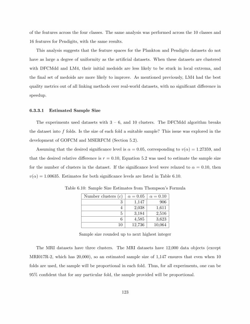
of the features across the four classes. The same analysis was performed across the 10 classes and
16 features for Pendigits, with the same results.
This analysis suggests that the feature spaces for the Plankton and Pendigits datasets do not
have as large a degree of uniformity as the artificial datasets. When these datasets are clustered
with DFCMdd and LM4, their initial medoids are less likely to be stuck in local extrema, and
the final set of medoids are more likely to improve. As mentioned previously, LM4 had the best
quality metrics out of all linking methods over real-world datasets, with no significant difference in
speedup.
6.3.3.1 Estimated Sample Size
The experiments used datasets with 3 – 6, and 10 clusters. The DFCMdd algorithm breaks
the dataset into f folds. Is the size of each fold a suitable sample? This issue was explored in the
development of GOFCM and MSERFCM (Section 5.2).
Assuming that the desired significance level is α = 0.05, corresponding to v(α) = 1.27359, and
that the desired relative difference is r = 0.10, Equation 5.2 was used to estimate the sample size
for the number of clusters in the dataset. If the significance level were relaxed to α = 0.10, then
v(α) = 1.00635. Estimates for both significance levels are listed in Table 6.10.
Table 6.10: Sample Size Estimates from Thompson’s Formula
Number clusters (c) α = 0.05 α = 0.10
3 1,147 906
4 2,038 1,611
5 3,184 2,516
6 4,585 3,623
10 12,736 10,064
Sample size rounded up to next highest integer
The MRI datasets have three clusters. The MRI datasets have 12,000 data objects (except
MRI017R-2, which has 20,000), so an estimated sample size of 1,147 ensures that even when 10
folds are used, the sample will be proportional in each fold. Thus, for all experiments, one can be
95% confident that for any particular fold, the sample provided will be proportional.
123
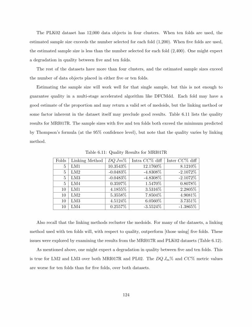
The PLK02 dataset has 12,000 data objects in four clusters. When ten folds are used, the
estimated sample size exceeds the number selected for each fold (1,200). When five folds are used,
the estimated sample size is less than the number selected for each fold (2,400). One might expect
a degradation in quality between five and ten folds.
The rest of the datasets have more than four clusters, and the estimated sample sizes exceed
the number of data objects placed in either five or ten folds.
Estimating the sample size will work well for that single sample, but this is not enough to
guarantee quality in a multi-stage accelerated algorithm like DFCMdd. Each fold may have a
good estimate of the proportion and may return a valid set of medoids, but the linking method or
some factor inherent in the dataset itself may preclude good results. Table 6.11 lists the quality
results for MRI017R. The sample sizes with five and ten folds both exceed the minimum predicted
by Thompson’s formula (at the 95% confidence level), but note that the quality varies by linking
method.
Table 6.11: Quality Results for MRI017R
Folds Linking Method DQJm% Intra CC% diff Inter CC% diff
5 LM1 10.3543% 12.1760% 8.1210%
5 LM2 -0.0483% -4.8308% -2.1072%
5 LM3 -0.0483% -4.8308% -2.1072%
5 LM4 0.3597% 1.5470% 0.8078%
10 LM1 4.1855% 3.5316% 2.2805%
10 LM2 5.3558% 7.8504% 4.9081%
10 LM3 4.5124% 6.0560% 3.7351%
10 LM4 0.2557% -3.5524% -1.3865%
Also recall that the linking methods recluster the medoids. For many of the datasets, a linking
method used with ten folds will, with respect to quality, outperform [those using] five folds. These
issues were explored by examining the results from the MRI017R and PLK02 datasets (Table 6.12).
As mentioned above, one might expect a degradation in quality between five and ten folds. This
is true for LM2 and LM3 over both MRI017R and PL02. The DQJm% and CC% metric values
are worse for ten folds than for five folds, over both datasets.
124
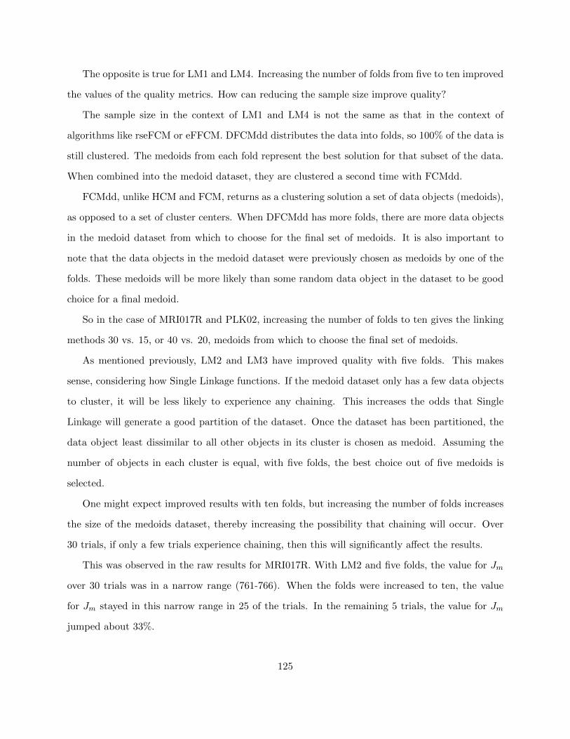
The opposite is true for LM1 and LM4. Increasing the number of folds from five to ten improved
the values of the quality metrics. How can reducing the sample size improve quality?
The sample size in the context of LM1 and LM4 is not the same as that in the context of
algorithms like rseFCM or eFFCM. DFCMdd distributes the data into folds, so 100% of the data is
still clustered. The medoids from each fold represent the best solution for that subset of the data.
When combined into the medoid dataset, they are clustered a second time with FCMdd.
FCMdd, unlike HCM and FCM, returns as a clustering solution a set of data objects (medoids),
as opposed to a set of cluster centers. When DFCMdd has more folds, there are more data objects
in the medoid dataset from which to choose for the final set of medoids. It is also important to
note that the data objects in the medoid dataset were previously chosen as medoids by one of the
folds. These medoids will be more likely than some random data object in the dataset to be good
choice for a final medoid.
So in the case of MRI017R and PLK02, increasing the number of folds to ten gives the linking
methods 30 vs. 15, or 40 vs. 20, medoids from which to choose the final set of medoids.
As mentioned previously, LM2 and LM3 have improved quality with five folds. This makes
sense, considering how Single Linkage functions. If the medoid dataset only has a few data objects
to cluster, it will be less likely to experience any chaining. This increases the odds that Single
Linkage will generate a good partition of the dataset. Once the dataset has been partitioned, the
data object least dissimilar to all other objects in its cluster is chosen as medoid. Assuming the
number of objects in each cluster is equal, with five folds, the best choice out of five medoids is
selected.
One might expect improved results with ten folds, but increasing the number of folds increases
the size of the medoids dataset, thereby increasing the possibility that chaining will occur. Over
30 trials, if only a few trials experience chaining, then this will significantly affect the results.
This was observed in the raw results for MRI017R. With LM2 and five folds, the value for Jm
over 30 trials was in a narrow range (761-766). When the folds were increased to ten, the value
for Jm stayed in this narrow range in 25 of the trials. In the remaining 5 trials, the value for Jm
jumped about 33%.
125
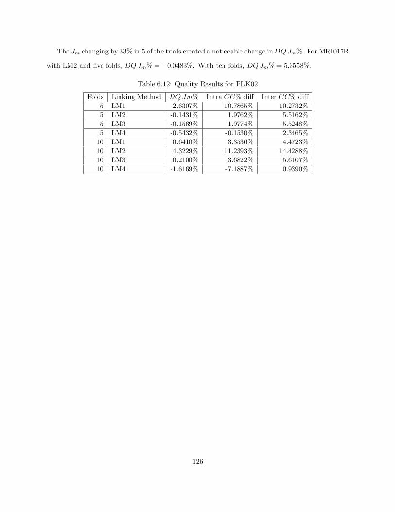
The Jm changing by 33% in 5 of the trials created a noticeable change inDQJm%. For MRI017R
with LM2 and five folds, DQJm% = −0.0483%. With ten folds, DQJm% = 5.3558%.
Table 6.12: Quality Results for PLK02
Folds Linking Method DQJm% Intra CC% diff Inter CC% diff
5 LM1 2.6307% 10.7865% 10.2732%
5 LM2 -0.1431% 1.9762% 5.5162%
5 LM3 -0.1569% 1.9774% 5.5248%
5 LM4 -0.5432% -0.1530% 2.3465%
10 LM1 0.6410% 3.3536% 4.4723%
10 LM2 4.3229% 11.2393% 14.4288%
10 LM3 0.2100% 3.6822% 5.6107%
10 LM4 -1.6169% -7.1887% 0.9390%
126

Chapter 7: Accelerating FN-DBSCAN
“If the world were perfect, it wouldn’t be.” - Lawrence “Yogi” Berra [2]
7.1 Accelerating a Density-Based Algorithm
The strategy of breaking a dataset into subsets can also be used to accelerate FN-DBSCAN. The
Accelerated FN-DBSCAN algorithm (AFN-DBSCAN) borrows from OFCM, DBDC, and SDBDC
[65] [74] [75]. In the OFCM algorithm, the fuzzy centroids retained from clustering each subset
represent the density of the dataset up to that point of the processing. The DBDC and SDBDC
algorithms do not fully leverage this idea, instead choosing the discrete values for “covering points”
and “covering radius” as a proxy for density.9
One clever idea from DBDC is the retention of a set of data objects not within ε distance of each
other, in order to sample the data evenly. This is a powerful idea, which is used in AFN-DBSCAN.
The AFN-DBSCAN algorithm combines these two ideas by breaking the dataset into subsets,
and by retaining weighted data objects to represent samples of the density in each subset. The
representative data objects from each subset are combined, and a weighted version of FN-DBSCAN
(WFN-DBSCAN) clusters that set of representative data objects. A final extension step assigns
all data objects from the original dataset to clusters. AFN-DBSCAN is formally presented as
Algorithm 10.
A significant departure from previous work in accelerating DBSCAN [74] [75] is that MinCard
is not defined as an integer, but as a real number. There is no reason for the minimum cardinality
9Some of the material in this chapter has been previously published by me [21] and is re-used under terms ofthe copyright c© 2010 IEEE. The name of the algorithm was changed to conform with the rest of this work. Newmaterial and analysis has been added.
127

of a fuzzy set to be restricted to an integer, and it was found in the course of experimentation that
for low density clusters, a real value for MinCard improved performance.
Algorithm 10: Accelerated FN-DBSCAN
1: Input: X, ε, MinCard, µ, f2: Break X into f equal sized subsets, X[k] : 1 ≤ k ≤ f . Randomly assign each xi ∈ X to a
subset.3: MaxRetained = n
f2
4: for all X[k] ⊂ X do5: Calculate FSCard(xi) (Equation 2.13) ∀i ∈ X[k]6: Add tuple (xi, FSCard(xi)) to RetainedListk where FSCard(xi) is the maximum in
X[k]7: while |RetainedListk| < MaxRetained do8: Add tuple (xi, FSCard(xi)) to RetainedListk where FSCard(xi) is the maximum in
X[k] not within ε distance of xj ∈ RetainedListk9: end while
10: end for11: Combine all tuples from RetainedListk : 1 ≤ k ≤ f into the combined weighted dataset,
W . Each FSCard(xi) value in a tuple serves as the weight, wi.12: Cluster W with WFN-DBSCAN using ε and MinCard.13: Obtain set of “core points” from WFN-DBSCAN.14: Assign clusters to all data objects xi ∈ X using the set of “core points”.
where:X is a dataset consisting of n data objects.ε is a distance.MinCard is a real number.µ is the fuzzy neighborhood function.f is the number of subsets.FSCard(xi) is the local density at a data object.
The WFN-DBSCAN algorithm is identical to FN-DBSCAN except for one detail. Instead of
FSCard(xi), the density at each data object is calculated with wFSCard(xi):
wFSCard(xi) =
n∑j=1
wi µ(xi, xj) (7.1)
128
where:
X is a dataset consisting of n data objects.
wi is the weight of xi.
µ is the fuzzy neighborhood function.
The average runtime complexity for DBSCAN and FN-DBSCAN is O(n2) with respect to the
number of data objects [24]. As the strategy to accelerate the algorithm is equivalent to that used
for DFCMdd, the runtime complexity analysis is the same (Section 6.1.3). Intuitively, the speedup
should be proportional to the number of subsets.
7.2 Experiments
The AFN-DBSCAN algorithm’s speed and performance were tested against FN-DBSCAN’s
on six real world datasets from the UCI repository (Chapter 3). The FN-DBSCAN algorithm is
deterministic, if the order of the data objects does not change. AFN-DBSCAN produces different
results, depending on how the dataset is divided into subsets. Each experiment consisted of 30
trials of AFN-DBSCAN, each with a different subset composition.
To calculate the speedup (SU), AFN-DBSCAN’s runtime was averaged over 30 trials and com-
pared to the runtime of FN-DBSCAN. AFN-DBSCAN’s fidelity to FN-DBSCAN was measured by
the average CC% from the results of FN-DBSCAN for the same dataset. The clusters were aligned
visually.
Wherever feasible, each dataset was broken into 6 subsets for clustering. For small datasets,
this was unrealistic. I set a minimum threshold of 70 data objects per subset, and that resulted in
two datasets having fewer than 6 subsets.
One difficulty in comparing AFN-DBSCAN and FN-DBSCAN is the setting of the parameter
MinCard. Using the same setting for MinCard for both algorithms caused AFN-DBSCAN to
have relatively inferior performance. While the representative data objects used by AFN-DBSCAN
were weighted, the actual spatial orientation of the representative data objects was lost. The need
to compensate for the loss of spatial orientation was discussed in the development of DBDC and
129

SDBDC [74] [75]. The strategy used in experimentation was to select MinCard for FN-DBSCAN
and to use a reduced value, rMinCard, for AFN-DBSCAN. This issue is fully discussed in Section
7.4.1.
Proper setting of parameters was challenging. The parameters were tuned by hand for FN-
DBSCAN to ensure that clusters were created when using the entire dataset. As a result, each
dataset had a different set of parameters. These are listed in Table 7.1. The linear membership
function was used for all experiments.
Table 7.1: AFN-DBSCAN Parameters
Dataset ε MinCard rMinCard
Breast Cancer-W 0.16 6 2.15
Heart-Statlog 0.30 8 2.60
Iris 0.20 6 2.15
Pendigits-015 0.1666 4 1.68
Letters-AY 0.15 28 6.46
Vote 0.45 6 2.15
7.3 Results
Results are shown in Table 7.2. Speedup varied from 2.91 to 4.70. The CC% varied from 0.37%
to 21.56%. The largest dataset, Pendigits015, was used to study how speedup and CC% varied
as the number of subsets changed. An additional series of experiments clustered the Pendigits015
dataset with 6, 8, 10, 12, and 16 subsets. Table 7.3 shows how the speedup and CC% increased
with the number of subsets.
The fidelity of the clustering to FN-DBSCAN, as measured by CC%, varied between 0.75% to
21.56%. The cause of this large degree of difference is discussed in Sections 7.4.1 and 7.4.2.
7.4 Discussion
This algorithm had unique challenges due to its dependance on density. Many of the datasets
clustered by AFN-DBSCAN had very “sparse” density, i.e., a relatively low ratio of data objects to
features. When a sparse dataset is broken into subsets, the distances between data objects are so
130
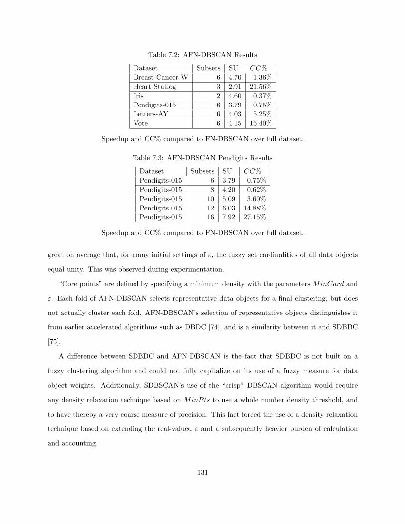
Table 7.2: AFN-DBSCAN Results
Dataset Subsets SU CC%
Breast Cancer-W 6 4.70 1.36%
Heart Statlog 3 2.91 21.56%
Iris 2 4.60 0.37%
Pendigits-015 6 3.79 0.75%
Letters-AY 6 4.03 5.25%
Vote 6 4.15 15.40%
Speedup and CC% compared to FN-DBSCAN over full dataset.
Table 7.3: AFN-DBSCAN Pendigits Results
Dataset Subsets SU CC%
Pendigits-015 6 3.79 0.75%
Pendigits-015 8 4.20 0.62%
Pendigits-015 10 5.09 3.60%
Pendigits-015 12 6.03 14.88%
Pendigits-015 16 7.92 27.15%
Speedup and CC% compared to FN-DBSCAN over full dataset.
great on average that, for many initial settings of ε, the fuzzy set cardinalities of all data objects
equal unity. This was observed during experimentation.
“Core points” are defined by specifying a minimum density with the parameters MinCard and
ε. Each fold of AFN-DBSCAN selects representative data objects for a final clustering, but does
not actually cluster each fold. AFN-DBSCAN’s selection of representative objects distinguishes it
from earlier accelerated algorithms such as DBDC [74], and is a similarity between it and SDBDC
[75].
A difference between SDBDC and AFN-DBSCAN is the fact that SDBDC is not built on a
fuzzy clustering algorithm and could not fully capitalize on its use of a fuzzy measure for data
object weights. Additionally, SDBSCAN’s use of the “crisp” DBSCAN algorithm would require
any density relaxation technique based on MinPts to use a whole number density threshold, and
to have thereby a very coarse measure of precision. This fact forced the use of a density relaxation
technique based on extending the real-valued ε and a subsequently heavier burden of calculation
and accounting.
131

AFN-DBSCAN samples the search space to the greatest extent possible. Only the least dense
portions of the search space are not represented. This was verified during implementation; in some
subsets, it was not possible to add MaxRetained tuples to RetainedList. Fewer data objects were
capable of covering all the data objects in the subset.
7.4.1 Reducing MinCard
The parameters MinCard and ε must be tuned for each dataset. There is a technique described
in [24] that works well on the crisp version of DBSCAN, but no similar technique has been developed
for FN-DBSCAN. As a result, the parameters were set via trial and error using FN-DBSCAN. It was
discovered that using the same measure for MinCard with both FN-DBSCAN and AFN-DBSCAN
resulted in dissimilar clusters. I solved this problem by reducing the setting for MinCard with
AFN-DBSCAN.
Reduction of MinCard was found to improve the concurrence of cluster assignments between
AFN-DBSCAN and FN-DBSCAN. This is a concept similar to extending ε in DBDC and SDBDC
[74] [75]. Both increasing ε and reducing MinCard have the effect of lowering the density require-
ments for cluster formation.
While this issue has nothing to do with either FN-DBSCAN or AFN-DBSCAN, it must ad-
dressed in order to compare the two algorithms experimentally.
Density requirements must be relaxed for the accelerated algorithms that use weighted repre-
sentative objects. These data objects represent many others through their weights, but the actual
locations of the represented data objects are lost. This loss of data makes the model cruder and
requires compensation.
The location of the original data objects is helpful to link representative objects together and
to create larger clusters. Loss of this spatial orientation makes cluster discovery less likely. The
strategy of increasing ε makes it more likely that a representative object will discover an adjacent
representative object. The disadvantage is the assumption that the adjacent representative object
actually will represent any data objects within the original ε distance. For datasets where clusters
have a small buffer between them, to increase ε may result in improperly combined clusters.
132
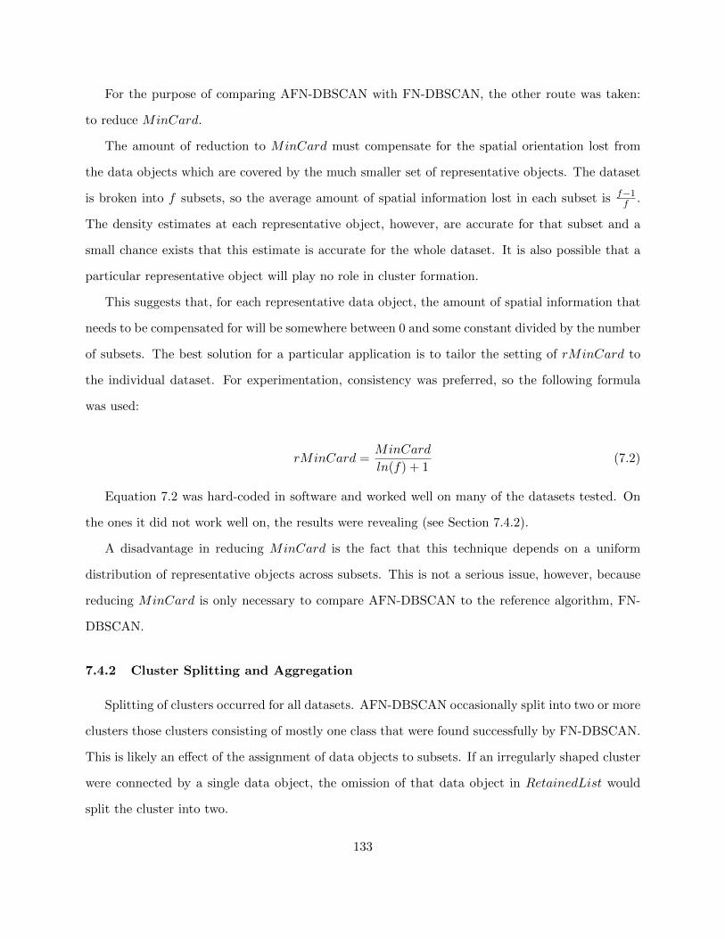
For the purpose of comparing AFN-DBSCAN with FN-DBSCAN, the other route was taken:
to reduce MinCard.
The amount of reduction to MinCard must compensate for the spatial orientation lost from
the data objects which are covered by the much smaller set of representative objects. The dataset
is broken into f subsets, so the average amount of spatial information lost in each subset is f−1f .
The density estimates at each representative object, however, are accurate for that subset and a
small chance exists that this estimate is accurate for the whole dataset. It is also possible that a
particular representative object will play no role in cluster formation.
This suggests that, for each representative data object, the amount of spatial information that
needs to be compensated for will be somewhere between 0 and some constant divided by the number
of subsets. The best solution for a particular application is to tailor the setting of rMinCard to
the individual dataset. For experimentation, consistency was preferred, so the following formula
was used:
rMinCard =MinCard
ln(f) + 1(7.2)
Equation 7.2 was hard-coded in software and worked well on many of the datasets tested. On
the ones it did not work well on, the results were revealing (see Section 7.4.2).
A disadvantage in reducing MinCard is the fact that this technique depends on a uniform
distribution of representative objects across subsets. This is not a serious issue, however, because
reducing MinCard is only necessary to compare AFN-DBSCAN to the reference algorithm, FN-
DBSCAN.
7.4.2 Cluster Splitting and Aggregation
Splitting of clusters occurred for all datasets. AFN-DBSCAN occasionally split into two or more
clusters those clusters consisting of mostly one class that were found successfully by FN-DBSCAN.
This is likely an effect of the assignment of data objects to subsets. If an irregularly shaped cluster
were connected by a single data object, the omission of that data object in RetainedList would
split the cluster into two.
133
Splitting is most likely to occur for datasets with very sparse density; i.e., datasets with a low
number of data objects and a large number of features. In the case of Pendigits-015 and Letters-AY,
the data described handwritten characters. Here, the splitting into multiple clusters might be an
inadvertent differentiation between slightly different styles of writing the same character.
Splitting occurred in a small percentage (< 15%) of trials in the experiments. When splitting
occurred, only the largest split cluster was counted when calculating CC%. The smaller clusters
were considered noise. It would have been possible to recombine sub-clusters manually for the
experimental results, but this was not done. Had this step been performed, CC% would have fallen
for all datasets.
The percentage of trials where splitting occurred was not uniform across the datasets. The
Heart-Statlog dataset had splitting occur in 60% of its trials. The splitting affected the results
profoundly; its CC% = 21.56% which was the highest any dataset. Note that Heart-Statlog has 13
features, but only 270 data objects.
Aggregation of clusters, i.e., multiple clusters in FN-DBSCAN combined into one by AFN-
DBSCAN, happened less frequently than splitting. Only the Heart Statlog, Letters-AY, and Vote
datasets had aggregated clusters. Aggregation appeared to be caused by the density relaxation,
i.e., the reduction of MinCard. When MinCard was not adjusted, aggregation did not occur.
The Vote dataset was the most impacted by aggregation; it occurred in 17% of its trials. As
a result of aggregation, Vote’s CC% = 15.40%. If trials where aggregation occurred were omitted
from the results, the CC% would have been 7.29%. This dataset was impacted by splitting as well,
which occurred in (a different) 17% of its trials.
7.4.3 Selecting the Number of Subsets
One decision that was made before using AFN-DBSCAN for experiments was the selection of
the number of subsets. For a real-world application where the data is geographically distributed,
this decision can be implicit, but it is still useful to demonstrate how speed and fidelity vary with
the number of subsets.
134
A small experiment was conducted using the Pendigits-015 dataset and five different subset
settings. The results are shown in Table 7.3. As expected from the runtime complexity, the
speedup improved as the number of subsets increased.
However, the fidelity to FN-DBSCAN, as measured by CC%, quickly degraded as the number of
subsets increased. While increasing from 6 to 8 subsets, slightly improved the fidelity, it degraded
when the number of subsets were 10 or greater.
The causes were splitting and noise. As explained in Section 7.4.2, as the number of subsets
increased, the spatial locations of data objects needed to join clusters were lost. This resulted in
increased splitting. When the number of subsets were set to 10, 13% of the trials experienced
splitting. When the number of subsets increased to 12, 77% of the trials experienced splitting and
when the number of subsets equalled 16, 100% of the clusters were split.
As explained above, a harsh criterion was used for calculating CC%. Only the largest cluster was
counted. Had all majority clusters for a class been counted, the reported fidelity to FN-DBSCAN
would have improved.
Changing the calculation of CC% would not have helped the second issue: noise. The loss of
spatial information when the subsets were 10 or greater also increased the amount of noise in each
trial. When the number of subsets was set to 10, 1.45% of the CC% of 3.60% was attributable to
noise. When the number of subsets increased to 12, 2.37% of the CC% of 14.88% was attributable to
noise, and when the number of subsets was set to 16, 3.95% of the CC% of 27.15% was attributable
to noise.
For this particular dataset, noise % did increase with the number of subsets, but cluster splitting
had a much greater effect.
7.4.4 Conclusions
The application of representative objects to accelerate a density-based algorithm has challenges
that do not exist for algorithms that reduce an objective function. Spatial information is lost when
representative objects are chosen and the location of the missing objects is often critical for proper
clustering.
135

In the case of the DBSCAN family of algorithms, the density is defined by the parameters ε
and MinCard. A difficulty was identified when a strategy was developed to compare the partitions
of FN-DBSCAN and AFN-DBSCAN. Recall that the parameters were originally tuned to FN-
DBSCAN, but using the same value for MinCard (assuming ε is kept constant) for FN-DBSCAN
and AFN-DBSCAN resulted in dissimilar partitions.
Clearly, different tuning measures are needed for AFN-DBSCAN than FN-DBSCAN. MinCard,
of course could have been hand-tuned for each dataset. Instead, a simple formula that generated
rMinCard from MinCard was consistently used in order to study this difficulty.
This formula worked well for many of the datasets, but not for others. The Heart-Statlog and
Vote datasets showed poor fidelity to FN-DBSCAN when clustered by AFN-DBSCAN, when the
simple formula was used to generate rMinCard. This led to the discovery that improper selection
of rMincard for AFN-DBSCAN can lead to splitting or aggregation. If all other factors are kept
equal, the intrinsic structure of a dataset plays a factor in fidelity to FN-DBSCAN as measured by
CC%.
Datasets often have sparse density, and breaking the dataset into subsets exacerbates the sparse-
ness. Additional experiments with Pendigits015, demonstrated the effects of increased sparseness
as the number of subsets was increased. There were increased instances of cluster splitting and an
increase in data objects improperly assigned the “noise” label.
This suggests that compensating for the loss of spatial information cannot be achieved by the use
of representative objects alone. A high-fidelity accelerated density-based algorithm must capture
key elements of cluster structure beyond that which is inferred by the representative objects. This
is an area for future research.
136

Chapter 8: Summary and Conclusions
“It ain’t over ’til it’s over.” - - Lawrence “Yogi” Berra [2]
8.1 Summary
In this dissertation, I explored the key algorithm design principles that accelerate fuzzy cluster-
ing algorithms while preserving quality and fidelity to the original algorithm. My research led to
the following contributions:
• Identification of a statistical method never before used with accelerated fuzzy clustering al-
gorithms. This method estimates the minimum sample size required to represent each cluster
proportionally. I modified the statistical formula to make it compatible with clustering algo-
rithms.
The issue of how to estimate the sample size has rarely been addressed in relevant literature.
Thompson’s method estimates the minimum sample size to proportionally represent a pop-
ulation within an absolute range of values. I demonstrated that in the context of clustering
algorithms, the use of an absolute value is cumbersome. I adjusted the equation to use a
relative difference in proportion.
• Creation of an early stopping criterion for incremental or “single pass” algorithms. This
criterion determines the point at which processing additional data will have little added
benefit. This allows the clustering algorithm to terminate early, providing a greater speedup
with little loss in quality.
In the domain of classification models, the idea of incrementally processing a dataset is well-
known. The accuracy of the classification model is the obvious stopping criterion, allowing a
137
model to be created in a shorter amount of time. A similar method for incremental clustering
was not possible, as no analogous stopping criterion existed. I explored a large set of viable
alternative stopping criteria and discovered that one based on the change in cluster center
position worked best.
• Different methods of combining representative objects were explored using fuzzy clustering
algorithms which produce partitions by minimizing an objective function. I discovered that
the best method used information inherent from the intermediate results to improve quality
and speedup.
Four different methods to combine representative objects for FCMdd clustering were explored.
The method that had the best performance on real-world datasets used the medoids from one
of the subsets as an initialization for a subsequent clustering by FCMdd.
• I developed a new method to combine representative objects in the context of density-based
fuzzy clustering algorithms. The criteria to join representative objects is a user-defined,
real-valued minimum fuzzy cardinality.
Density-based clustering algorithms, have difficulty clustering subsets because the threshold
density will differ between the subsets and full dataset. In the context of accelerated fuzzy
neighborhood density-based clustering, I avoid the entire issue by retaining the densest set of
representative objects that minimize overlap. Experimentation led to the discovery that the
intrinsic structure of the dataset played a large factor in the accelerated algorithm’s fidelity
to the base algorithm.
• I created five original algorithms that apply these contributions and the four main ideas listed
above.
Thompson’s method estimates the minimum sample size for GOFCM and MSERFCM. Both
algorithms reduce runtime and minimize quality loss in comparison to the algorithms on
which they were based. GOFCM and MODSPFCM use the early stopping criterion to reduce
runtime while minimizing loss of quality. GOFCM, MODSPFCM, DFCMdd, and AFN-
138
DBSCAN all use representative objects to reduce runtime. This technique minimizes quality
loss, and occasionally improves the quality of results. AFN-DBSCAN implements a new
method to combine representative objects from a density-based clustering algorithm.
My original research on these subjects was published in two conference papers and two journal
papers [21] [22] [55] [23]. A disk with the source code developed for all research is included in
Appendix A.
8.2 Conclusions
This research is important, because clustering is a primary technique used in data analysis. The
vast amounts of Big Data available contain valuable information and insights. Such a huge quantity
of data cannot be clustered with traditional, basic methods. Accelerated clustering methods are
therefore needed. Fuzzy clustering is a valuable tool to the data analyst and should be incorporated
into clustering solutions.
The first step of the research was to study how existing accelerated fuzzy clustering methods
work. In addition to reviewing existing published research, I conducted a series of experiments
where I compared four accelerated fuzzy clustering algorithms to FCM. The experiments identified
the following principles:
1. Use of a statistically significant sample of the dataset reduces runtime while preserving quality.
2. An algorithm designed to cluster the data incrementally can produce a high-quality result
when stopped before all data has been processed. This is especially true when the data is
presented in random order.
3. The use of representative objects, either weighted or un-weighted, can overcome difficulties
of scale, if properly utilized.
4. For a particular class of clustering algorithms, providing a “starting point” close to the optimal
solution reduces runtime and can improve quality.
139
These design principles, present in existing algorithms, were already well-known. The signif-
icance of my experiments and the published results [22] was that such a comparative analysis of
FCM-based accelerated methods had not been previously published.10 Most published work is
limited to a single accelerated clustering method. Surveys on clustering methods typically do not
focus on accelerated methods [3] [112] [113], making it infrequent, if not unlikely, that all of these
principles were discussed in print simultaneously.
These design principles served as a nucleus for the study of how existing accelerated fuzzy clus-
tering algorithms could be improved further. In the course of my research, most of the algorithms
encountered used only one of these aforementioned principles. There is power in using multiple
design principles in tandem.
Thompson’s method of estimating a minimum sample size was useful in the context of GOFCM,
MSERFCM, and MODSPFCM where a single sample is relevant. The sample size must at least
proportionally represent the data to yield useful results. This is true if an estimate is needed either
for initialization or the final results.
These algorithms combined the use of a minimum, estimated sample size as well as some com-
bination of weighted representative objects, improved starting positions, and early termination
criterion. It was clearly shown that a combined approach outperformed related algorithms.
For algorithms such as OFCM and DFCMdd, the proportionality of the sample is less relevant
because the information inherent in the results from each PDA (or fold) is reused in order to obtain
a final clustering solution. Paradoxically, DFCMdd’s results showed that, on real-world data, a
smaller sample size for folds yielded faster clustering and higher quality.
Representative objects must be used in an intelligent fashion. With OFCM, I demonstrated that
using representative objects as an initialization can result in poorer performance, if the sample from
which they were derived does not proportionally represent the whole dataset. I used this concept
to implement acceleration strategies successfully for FCMdd.
The need to accelerate fuzzy clustering algorithms for Big Data motivated the identification of
these design principles and my contributions. In truth, I only scratched the surface of the potential
10Formal publication of my comparative analysis [22] preceded Havens’ [16] by six months, though the researchwas performed independently, at roughly the same time.
140

of these principles and contributions. The research presented in this dissertation can be continued
in a number of ways.
Reducing the fold size for DFCMdd was shown to improve speedup and quality for two of the
linking methods. I strongly suspect that this is only true over some range of fold sizes and other
factors. This is clearly an area for future study for ways to intelligently use representative objects
in DFCMdd, OFCM, and AFN-DBSCAN.
Weights were used for representative objects in GOFCM, MSERFCM, MODSPFCM and AFN-
DBSCAN, but not DFCMdd. A version of DFCMdd can be created with weighted medoids and the
performance between the two versions can be compared. Weights were shown to have advantages,
but also disadvantages in that they can skew results and not account for spatial information. This
was especially true for AFN-DBSCAN. An alternative means of compensating for loss of spatial
information is a future area of study.
The early stopping criterion can be applied to other clustering algorithms. Development of
a stopping criterion for relational data would make possible relational versions of GOFCM and
MODSPFCM. A relational version of MSERFCM could also be created with the contributions in
this dissertation.
This dissertation shows that the intelligent use of multiple design principles can accelerate fuzzy
clustering algorithms with minimal quality loss. With the principles identified and my original
contributions, I see the potential for the creation of many more useful clustering methods.
141
References
[1] Y. Berra, You Can Observe a Lot by Watching. John Wiley and Sons, 2008.
[2] ——, The Yogi Book:” I Really Didn’t Say Everything I Said”. Workman Publishing, 1998.
[3] A. K. Jain, “Data clustering: A review,” ACM Computing Surveys (CSUR), vol. 31, no. 3,pp. 264–323, September 1999.
[4] V. Estivill-Castro, “Why so many clustering algorithms: a position paper,” ACM SIGKDDExplorations Newsletter, vol. 4, no. 1, pp. 65–75, 2002.
[5] A. K. Jain, “Data clustering: 50 years beyond k-means,” Pattern Recognition Letters, vol. 31,no. 8, pp. 651–666, June 2010.
[6] A. S. Das, M. Datar, A. Garg, and S. Rajaram, “Google news personalization: scalable onlinecollaborative filtering,” in Proceedings of the 16th international conference on World WideWeb. ACM, 2007, pp. 271–280.
[7] J. C. Russ, The image processing handbook. CRC press, 2011.
[8] R. N. Kostoff, M. B. Briggs, J. L. Solka, and R. L. Rushenberg, “Literature-related discovery(lrd): Methodology,” Technological Forecasting and Social Change, vol. 75, no. 2, pp. 186–202,2008.
[9] G. Punj and D. W. Stewart, “Cluster analysis in marketing research: review and suggestionsfor application,” Journal of marketing research, pp. 134–148, 1983.
[10] M. B. Eisen, P. T. Spellman, P. O. Brown, and D. Botstein, “Cluster analysis and display ofgenome-wide expression patterns,” Proceedings of the National Academy of Sciences, vol. 95,no. 25, pp. 14 863–14 868, 1998.
[11] P. Hore, L. O. Hall, D. B. Goldgof, Y. Gu, A. A. Maudsley, and A. Darkazanli, “A scalableframework for segmenting magnetic resonance images,” Journal of signal processing systems,vol. 54, no. 1-3, pp. 183–203, 2009.
[12] M. Benigni and R. Furrer, “Periodic spatio-temporal improvised explosive device attack pat-tern analysis,” Technical report, Golden, CO, Tech. Rep., 2008.
[13] M. Nikravesh, “Soft computing for reservoir characterization and management,” in GranularComputing, 2005 IEEE International Conference on, vol. 2. IEEE, 2005, pp. 593–598.
142
[14] D. B. Henry, P. H. Tolan, and D. Gorman-Smith, “Cluster analysis in family psychologyresearch.” Journal of Family Psychology, vol. 19, no. 1, p. 121, 2005.
[15] P. Huber, “Massive data sets workshop: The morning after.”
[16] T. C. Havens, J. C. Bezdek, C. Leckie, L. O. Hall, and M. Palaniswami, “Fuzzy c-meansalgorithms for very large data,” IEEE Trans. Fuzzy Systems, vol. 20, no. 6, pp. 1130–1146,December 2012.
[17] S. Lohr, “The age of big data,” New York Times, vol. 11, 2012.
[18] S. Madden, “From databases to big data,” Internet Computing, IEEE, vol. 16, no. 3, pp. 4–6,2012.
[19] A. Jacobs, “The pathologies of big data,” Communications of the ACM, vol. 52, no. 8, pp.36–44, 2009.
[20] B. Ratner, Statistical and machine-learning data mining: techniques for better predictivemodeling and analysis of big data. CRC Press, 2011.
[21] J. K. Parker, L. O. Hall, and A. Kandel, “Scalable fuzzy neighborhood dbscan,” in FuzzySystems (FUZZ-IEEE), 2010 IEEE International Conference on. IEEE, 2010, pp. 1–8.
[22] J. K. Parker, L. O. Hall, and J. C. Bezdek, “Comparison of scalable fuzzy clustering methods,”in Fuzzy Systems (FUZZ-IEEE), 2012 IEEE International Conference on. IEEE, 2012, pp.1–9.
[23] J. K. Parker and L. O. Hall, “Accelerating fuzzy c means using an estimated subsample size,”Fuzzy Systems, IEEE Transactions on, 2013.
[24] M. Ester, H.-P. Kriegel, J. Sander, and X. Xu, “A density-based algorithm for discoveringclusters in large spatial databases with noise.” Kdd, 1996.
[25] R. Sibson, “Slink: an optimally efficient algorithm for the single-link cluster method,” TheComputer Journal, vol. 16, no. 1, pp. 30–34, 1973.
[26] N. Jardine and R. Sibson, “The construction of hierarchic and non-hierarchic classifications,”The Computer Journal, vol. 11, no. 2, pp. 177–184, 1968.
[27] C. D. Manning, P. Raghavan, and H. Schutze, Introduction to information retrieval. Cam-bridge University Press Cambridge, 2008, vol. 1.
[28] L. Kaufman and P. J. Rousseeuw, Finding Groups in Data: An Introduction to ClusterAnalysis. Wiley-Interscience, 1990.
[29] Y. Loewenstein, E. Portugaly, M. Fromer, and M. Linial, “Efficient algorithms for accuratehierarchical clustering of huge datasets: tackling the entire protein space,” Bioinformatics,vol. 24, no. 13, pp. i41–i49, 2008.
[30] J. MacQueen et al., “Some methods for classification and analysis of multivariate observa-tions,” in Proceedings of the fifth Berkeley symposium on mathematical statistics and proba-bility, vol. 1, no. 281-297. California, USA, 1967, p. 14.
143
[31] S. Lloyd, “Least squares quantization in pcm,” Information Theory, IEEE Transactions on,vol. 28, no. 2, pp. 129–137, 1982.
[32] J. C. Bezdek, R. Ehrlich, and W. Full, “Fcm: The fuzzy c-means clustering algorithm,”Computers & Geosciences, vol. 10, no. 2, pp. 191–203, 1984.
[33] R. O. Duda, P. E. Hart, and D. G. Stork, Pattern classification. John Wiley & Sons, 2001.
[34] D. Aloise, A. Deshpande, P. Hansen, and P. Popat, “Np-hardness of euclidean sum-of-squaresclustering,” Machine Learning, vol. 75, no. 2, pp. 245–248, 2009.
[35] J. C. Bezdek and R. J. Hathaway, “Some notes on alternating optimization,” in Advances inSoft ComputingAFSS 2002. Springer, 2002, pp. 288–300.
[36] M. Matteucci, “A tutorial on clustering algorithms, clustering k-means demo,” http://home.deib.polimi.it/matteucc/Clustering/tutorial html/AppletKM.html, accessed: 2013-07-06.
[37] R. A. Jarvis and E. A. Patrick, “Clustering using a similarity measure based on shared nearneighbors,” Computers, IEEE Transactions on, vol. 100, no. 11, pp. 1025–1034, 1973.
[38] E. Parzen, “On estimation of a probability density function and mode,” The annals of math-ematical statistics, vol. 33, no. 3, pp. 1065–1076, 1962.
[39] N. Beckmann, H.-P. Kriegel, R. Schneider, and B. Seeger, “The r*-tree: an efficient androbust access method for points and rectangles,” in INTERNATIONAL CONFERENCE ONMANAGEMENT OF DATA. Citeseer, 1990.
[40] A. Kandel and W. Byatt, “Fuzzy sets, fuzzy algebra, and fuzzy statistics,” Proceedings of theIEEE, vol. 66, no. 12, pp. 1619–1639, 1978.
[41] J. C. Bezdek, Pattern Recognition with Fuzzy Objective Function Algorithms. Plenum Press,1981.
[42] I. Gath and A. B. Geva, “Unsupervised optimal fuzzy clustering,” Pattern Analysis andMachine Intelligence, IEEE Transactions on, vol. 11, no. 7, pp. 773–780, 1989.
[43] Z. Huang and M. K. Ng, “A fuzzy k-modes algorithm for clustering categorical data,” FuzzySystems, IEEE Transactions on, vol. 7, no. 4, pp. 446–452, 1999.
[44] R. Krishnapuram, A. Joshi, and L. Yi, “A fuzzy relative of the k-medoids algorithm with ap-plication to web document and snippet clustering,” in Fuzzy Systems Conference Proceedings,1999. FUZZ-IEEE’99. 1999 IEEE International, vol. 3. IEEE, 1999, pp. 1281–1286.
[45] E. N. Nasibov and G. Ulutagay, “Robustness of density-based clustering methods with variousneighborhood relations,” Fuzzy Sets and Systems, vol. 160, no. 24, pp. 3601–3615, 2009.
[46] P. Hore, L. O. Hall, and D. B. Goldgof, “Single pass fuzzy c means,” in IEEE InternationalConference on Fuzzy Systems. FUZZ-IEEE, July 2007, pp. 1–7.
[47] J. Kolen and T. Hutcheson, “Reducing the time complexity of the fuzzy c-means algorithm,”Fuzzy Systems, IEEE Transactions on, vol. 10, no. 2, pp. 263 –267, apr 2002.
144
[48] R. J. Hathaway, J. W. Davenport, and J. C. Bezdek, “Relational duals of the c-means clus-tering algorithms,” Pattern recognition, vol. 22, no. 2, pp. 205–212, 1989.
[49] R. J. Hathaway and J. C. Bezdek, “Nerf c-means: Non-euclidean relational fuzzy clustering,”Pattern recognition, vol. 27, no. 3, pp. 429–437, 1994.
[50] V. V. Vazirani, Approximation algorithms. springer, 2001.
[51] J. Han, M. Kamber, and J. Pei, Data mining: concepts and techniques. Morgan kaufmann,2006.
[52] R. Krishnapuram, A. Joshi, O. Nasraoui, and L. Yi, “Low-complexity fuzzy relational clus-tering algorithms for web mining,” Fuzzy Systems, IEEE Transactions on, vol. 9, no. 4, pp.595–607, 2001.
[53] K. S. Fu and J. E. Albus, Syntactic pattern recognition and applications. Prentice-HallEnglewood Cliffs, NJ, 1982, vol. 4.
[54] N. Labroche, “New incremental fuzzy c medoids clustering algorithms,” in Fuzzy InformationProcessing Society (NAFIPS), 2010 Annual Meeting of the North American. IEEE, 2010,pp. 1–6.
[55] J. K. Parker and J. A. Downs, “Footprint generation using fuzzy-neighborhood clustering,”GeoInformatica, pp. 1–15, 2013.
[56] E. N. Nasibov and G. Ulutagay, “On cluster analysis based on fuzzy relations between spatialdata.” in EUSFLAT Conf.(2). Citeseer, 2007, pp. 59–62.
[57] I. Guyon and A. Elisseeff, “An introduction to variable and feature selection,” The Journalof Machine Learning Research, vol. 3, pp. 1157–1182, 2003.
[58] H. Liu and L. Yu, “Toward integrating feature selection algorithms for classification andclustering,” Knowledge and Data Engineering, IEEE Transactions on, vol. 17, no. 4, pp.491–502, 2005.
[59] L. Parsons, E. Haque, and H. Liu, “Subspace clustering for high dimensional data: a review,”ACM SIGKDD Explorations Newsletter, vol. 6, no. 1, pp. 90–105, 2004.
[60] R. Agrawal, J. Gehrke, D. Gunopulos, and P. Raghavan, “Automatic subspace clusteringof high dimensional data,” Data Mining and Knowledge Discovery, vol. 11, no. 1, pp. 5–33,2005.
[61] P. S. Bradley and U. M. Fayyad, “Refining initial points for k-means clustering,” MicrosoftResearch, Tech. Rep. MSR-TR-98-36, May 1998.
[62] T. W. Cheng, D. B. Goldgof, and L. O. Hall, “Fast fuzzy clustering,” Fuzzy sets and systems,vol. 93, no. 1, pp. 49–56, 1998.
[63] D. Altman, “Efficient fuzzy clustering of multi-spectral images,” in Geoscience and RemoteSensing Symposium, 1999. IGARSS’99 Proceedings. IEEE 1999 International, vol. 3. IEEE,1999, pp. 1594–1596.
145
[64] M.-C. Hung and D.-L. Yang, “An efficient fuzzy c-means clustering algorithm,” in DataMining, 2001. ICDM 2001, Proceedings IEEE International Conference on. IEEE, 2001, pp.225–232.
[65] P. Hore, L. Hall, D. Goldgof, and W. Cheng, “Online fuzzy c means,” in Fuzzy InformationProcessing Society, 2008. NAFIPS 2008. Annual Meeting of the North American. IEEE,2008, pp. 1–5.
[66] F. Provost, D. Jensen, and T. Oates, “Efficient progressive sampling,” in Proceedings ofthe fifth ACM SIGKDD international conference on Knowledge discovery and data mining.ACM, 1999, pp. 23–32.
[67] P. Domingos, G. Hulten, P. Edu, and C. Edu, “A general method for scaling up machinelearning algorithms and its application to clustering,” in In Proceedings of the EighteenthInternational Conference on Machine Learning, 2001.
[68] N. R. Pal and J. C. Bezdek, “Complexity reduction for large image processing,” Systems,Man, and Cybernetics, Part B: Cybernetics, IEEE Transactions on, vol. 32, no. 5, pp. 598–611, 2002.
[69] L. Wang, J. C. Bezdek, C. Leckie, and R. Kotagiri, “Selective sampling for approximateclustering of very large data sets,” International Journal of Intelligent Systems, vol. 23, no. 3,pp. 313–331, 2008.
[70] J. C. Bezdek, R. J. Hathaway, J. M. Huband, C. Leckie, and R. Kotagiri, “Approximateclustering in very large relational data,” International journal of intelligent systems, vol. 21,no. 8, pp. 817–841, 2006.
[71] P. Hore, “Scalable frameworks and algorithms for cluster ensembles and clustering datastreams,” Ph.D. dissertation, University of South Florida, June 2007.
[72] R. J. Hathaway and J. C. Bezdek, “Extending fuzzy and probabilistic clustering to very largedata sets,” Computational Statistics & Data Analysis, vol. 51, no. 1, pp. 215–234, 2006.
[73] J. C. Bezdek and R. J. Hathaway, “Progressive sampling schemes for approximate cluster-ing in very large data sets,” in Fuzzy Systems, 2004. Proceedings. 2004 IEEE InternationalConference on, vol. 1. IEEE, 2004, pp. 15–21.
[74] E. Januzaj, H.-P. Kriegel, and M. Pfeifle, “Dbdc: Density based distributed clustering,” inAdvances in Database Technology-EDBT 2004. Springer, 2004, pp. 88–105.
[75] ——, “Scalable density-based distributed clustering,” in Knowledge Discovery in Databases:PKDD 2004. Springer, 2004, pp. 231–244.
[76] N. Webster and J. L. McKechnie, Webster’s new universal unabridged dictionary. Dorset &Baber, 1983.
[77] Y. Gu, L. O. Hall, and D. B. Goldgof, “Evaluating scalable fuzzy clustering,” in Systems Manand Cybernetics (SMC), 2010 IEEE International Conference on. IEEE, 2010, pp. 873–880.
146
[78] R. J. Hathaway and J. C. Bezdek, “Optimization of clustering criteria by reformulation,”Fuzzy Systems, IEEE Transactions on, vol. 3, no. 2, pp. 241–245, 1995.
[79] H. W. Kuhn, “The hungarian method for the assignment problem,” Naval Research LogisticsQuarterly, vol. 2, no. 1-2, pp. 83–97, March 1955.
[80] W. M. Rand, “Objective criteria for the evaluation of clustering methods,” Journal of theAmerican Statistical association, vol. 66, no. 336, pp. 846–850, 1971.
[81] J. M. Santos and M. Embrechts, “On the use of the adjusted rand index as a metric forevaluating supervised classification,” in Artificial Neural Networks–ICANN 2009. Springer,2009, pp. 175–184.
[82] L. Hubert and P. Arabie, “Comparing partitions,” Journal of classification, vol. 2, no. 1, pp.193–218, 1985.
[83] J. L. Myers, A. D. Well, and R. F. Lorch, Research design and statistical analysis. Routledge,2010.
[84] R. Walpole and R. Myers, Probability and Statistics for Engineers and Scientists. MacMillanPublishing Company, 1985.
[85] S. Samson, T. Hopkins, A. Remsen, L. Langebrake, T. Sutton, and J. Patten, “A system forhigh-resolution zooplankton imaging,” Oceanic Engineering, IEEE Journal of, vol. 26, no. 4,pp. 671–676, 2001.
[86] A. Remsen, T. L. Hopkins, and S. Samson, “What you see is not what you catch: a comparisonof concurrently collected net, optical plankton counter, and shadowed image particle profilingevaluation recorder data from the northeast gulf of mexico,” Deep Sea Research Part I:Oceanographic Research Papers, vol. 51, no. 1, pp. 129–151, 2004.
[87] K. A. Kramer, “System for identifying plankton from the sipper instrument platform,” Ph.D.dissertation, University of South Florida, 2010.
[88] M. Hall, E. Frank, G. Holmes, B. Pfahringer, P. Reutemann, and I. H. Witten, “The wekadata mining software: an update,” ACM SIGKDD Explorations Newsletter, vol. 11, no. 1,pp. 10–18, 2009.
[89] H. Liu and R. Setiono, “A probabilistic approach to feature selection-a filter solution,” inICML, vol. 96. Citeseer, 1996, pp. 319–327.
[90] J. Liang, L. Bai, C. Dang, and F. Cao, “The k-means-type algorithms versus imbalanced datadistributions,” IEEE Transactions on Fuzzy Systems, vol. 20, no. 4, pp. 728–745, 2012.
[91] J. C. Bezdek, R. J. Hathaway, M. J. Sabin, and W. T. Tucker, “Convergence theory for fuzzyc-means: counterexamples and repairs,” Systems, Man and Cybernetics, IEEE Transactionson, vol. 17, no. 5, pp. 873–877, 1987.
[92] K. Bache and M. Lichman, “UCI machine learning repository,” 2013. [Online]. Available:http://archive.ics.uci.edu/ml
147
[93] W. H. Wolberg and O. L. Mangasarian, “Multisurface method of pattern separation formedical diagnosis applied to breast cytology.” Proceedings of the national academy of sciences,vol. 87, no. 23, pp. 9193–9196, 1990.
[94] C. Feng, A. Sutherland, R. King, S. Muggleton, and R. Henery, “Comparison of machinelearning classifiers to statistics and neural networks,” AI&Statistics-93, vol. 6, p. 41, 1993.
[95] R. A. Fisher, “The use of multiple measurements in taxonomic problems,” Annals of eugenics,vol. 7, no. 2, pp. 179–188, 1936.
[96] A. Srinivasan. (1993) Statlog (landsat satellite) data set. Repository. [Online]. Available:http://archive.ics.uci.edu/ml/datasets/Statlog+%28Landsat+Satellite%29
[97] P. W. Frey and D. J. Slate, “Letter recognition using holland-style adaptive classifiers,”Machine Learning, vol. 6, no. 2, pp. 161–182, 1991.
[98] F. Alimoglu and E. Alpaydin, “Methods of combining multiple classifiers based on differentrepresentations for pen-based handwritten digit recognition,” in Proceedings of the Fifth Turk-ish Artificial Intelligence and Artificial Neural Networks Symposium (TAINN 96). Citeseer,June 1996.
[99] J. C. Schlimmer, “Concept acquisition through representational adjustment,” Ph.D. disser-tation, University of California, Irvine, 1987.
[100] S. Eschrich, J. Ke, L. O. Hall, and D. B. Goldgof, “Fast accurate fuzzy clustering throughdata reduction,” Fuzzy Systems, IEEE Transactions on, vol. 11, no. 2, pp. 262–270, 2003.
[101] B. Gu, B. Liu, F. Hu, and H. Liu, “Efficiently determining the starting sample size forprogressive sampling,” in Machine Learning: ECML 2001. Springer, 2001, pp. 192–202.
[102] S. K. Thompson, “Sample size for estimating multinomial proportions,” The American Statis-tician, vol. 41, no. 1, pp. 42–46, 1987.
[103] P. Phoungphol and Y. Zhang, “Sample size estimation with high confidence for large scaleclustering,” in Proceedings of the 3rd International Conference on Intelligent Computing andIntelligent Systems, 2011.
[104] C. Meek, B. Thiesson, and D. Heckerman, “The learning-curve sampling method applied tomodel-based clustering,” The Journal of Machine Learning Research, vol. 2, pp. 397–418,2002.
[105] L. O. Hall and D. B. Goldgof, “Convergence of the single-pass and online fuzzy c-meansalgorithms,” Fuzzy Systems, IEEE Transactions on, vol. 19, no. 4, pp. 792–794, 2011.
[106] T. C. Havens, private communication, 2012.
[107] L. P. Clarke, R. P. Velthuizen, M. Clark, J. Gaviria, L. O. Hall, D. Goldgof, R. Murtagh,S. Phuphanich, and S. Brem, “Mri measurement of brain tumor response: comparison ofvisual metric and automatic segmentation,” Magnetic resonance imaging, vol. 16, no. 3, pp.271–279, 1998.
148
[108] M. Emre Celebi, H. A. Kingravi, and P. A. Vela, “A comparative study of efficient initial-ization methods for the k-means clustering algorithm,” Expert Systems with Applications,2012.
[109] A. Strehl and J. Ghosh, “Cluster ensembles—a knowledge reuse framework for combiningmultiple partitions,” The Journal of Machine Learning Research, vol. 3, pp. 583–617, 2003.
[110] J. Mei and L. Chen, “Fuzzy clustering with weighted medoids for relational data,” PatternRecognition, vol. 43, no. 5, pp. 1964–1974, 2010.
[111] R. P. Duin, M. Loog, E. Pe, kalska, and D. M. Tax, “Feature-based dissimilarity spaceclassification,” in Recognizing Patterns in Signals, Speech, Images and Videos. Springer,2010, pp. 46–55.
[112] R. Xu, D. Wunsch et al., “Survey of clustering algorithms,” Neural Networks, IEEE Trans-actions on, vol. 16, no. 3, pp. 645–678, 2005.
[113] P. Berkhin, “A survey of clustering data mining techniques,” in Grouping multidimensionaldata. Springer, 2006, pp. 25–71.
[114] B. Hoyt. (2011) inih: simple .ini parser in c. Open Source Project. [Online]. Available:http://code.google.com/p/inih/
[115] I. H. Witten and E. Frank, Data Mining: Practical machine learning tools and techniques.Morgan Kaufmann, 2005.
[116] B. Reiter and J. Aquino. (2009) Statist 1.4.2. Open Source Project. [Online]. Available:http://wald.intevation.org/projects/statist/
149

Appendices
150
Appendix A: Algorithm Implementations
“If you can’t imitate him, don’t copy him.” - Lawrence “Yogi” Berra [2]
A.1 Introduction
Three different codebases were developed to conduct experiments for my research. A disk is
provided with this dissertation with all source code and datasets.11
A.2 Fuzzy c-means Codebase
The Fuzzy c-means (FCM) codebase includes the implementations of FCM and the following
accelerated methods: SPFCM, OFCM, eFFCM, rseFCM, GOFCM, MSERFCM and MODSPFCM.
See Chapters 2 and 5 for details on the algorithms. All algorithmic variants used the same weighted
FCM implementation, written in C, and were compiled and run in a Linux environment. Original
implementations of FCM by Steven Eschrich [100] and SPFCM and OFCM by Prodip Hore [71]
were reviewed. Some implementation techniques were adopted, but the code was entirely rewritten.
Code from [114] was used for some utility functions.
All algorithms requiring a random number, typically for initialization or randomization, used a
custom function to generate a pseudo-random number in the range specified. This function used a
pair of pseudo-random numbers which were bit-shifted and the OR operator was applied to obtain a
32-bit number. To provide unique randomization, each trial in an experiment was issued a different
seed.
The following procedure for drawing a random sample was used for all algorithms. The dataset
is first loaded into memory, and pairs of data objects were randomly selected to be swapped. The
positions of data objects are swapped n× e times, where n is the number of data objects and e is
the natural logarithm base. The randomized version of the dataset in memory is then written to
disk. Algorithms requiring a random sample read the file sequentially to obtain the desired sample
11Some of the material in this chapter has been previously published by me [21] [22] [23], and is re-used underterms of the copyright c© 2010, 2012 and 2013 IEEE. New material and analysis has been added.
151
Appendix A (Continued)
size. For consistency, the eFFCM algorithm used the above method for sample selection, despite
[68] stating that selection should be made with replacement.
If the positions of pairs of data objects are swapped n×e times, the probability of a data object
not being swapped at least once is [115]:
(1− 1
n
)2ne
= 0.00435 (A.1)
as n approaches infinity. This ensures a probability greater than 99.5% that any given data object
will have its position altered. This is a reasonably high likelihood and motivated the selection of
n× e swaps.
The procedure used for random selection, while it may seem cumbersome, was intentional. The
randomized datasets were written to disk. This allowed subsequent experiments to use the same
samples of the data. This procedure also facilitated validation of the custom random number
generator.
A.2.1 Termination Criterion
The FCM algorithm terminates when the difference between successive matrices or successive
sets of cluster centers (as measured by a convenient matrix norm) falls below ε.
Given the goal of the research, a comparison of algorithms across multiple datasets, using a
matrix norm to compare either alternative is problematic. The dataset sizes, sizes of PDA, and
range of the data differ in each experiment. Fixing the parameter, ε, to a single value makes fair
comparison difficult.
For example, imagine comparing two successive U matrices by using the summation of differ-
ences between cluster memberships as the matrix norm. This can be tuned for a single algorithm,
but the same value for ε cannot be used as termination criterion to compare FCM and SPFCM.
The dataset size is n for FCM, but fPDA × n for SPFCM. To obtain an equal value of ε, FCM
152
Appendix A (Continued)
would require a smaller average difference in individual u values than would SPFCM, increasing its
runtime.
Comparing V matrices has the same problem as described above when one wishes to compare
performance across different datasets with different numbers of clusters. Using the same value for
ε would require higher quality results from datasets with more clusters and permit lower quality
results from datasets with fewer clusters. Another difficulty in using a V norm is that different
datasets have different ranges of data. This makes relative quality of results dependent on the
dataset. Scaling the data would correct this one issue, if one wished to compare datasets with the
same number of clusters.
The solution is to use the U matrix sup norm, which is less dependent on the dataset size, scale,
or number of clusters. In my research, the termination criterion used the maximum difference,
maxChange, in the U matrix sup norm. If the maximum membership value for a data object
in successive Us fell below the value for ε, the algorithm terminated. As this criterion tests the
stability of the membership values, it is independent of dataset size and data scale. While the
effects due to number of clusters are unknown, this technique provides a clear and unambiguous
stopping criterion.
This leaves the question of how to initialize FCM. It is possible to initialize either the V matrix
or the U matrix. The technique described in earlier accelerated fuzzy clustering work was used [62]
[64]. The V matrix is initialized by randomly selecting c data objects from the input dataset. The
U membership matrix was then initialized by calling the function that executed Equation (2.8)
above. We then iterated V and U until termination.
As discussed above, the software implementation calculates the maximum difference in mem-
bership value (maxChange) for a data object in X while Equation (2.8) is executed. The stopping
criterion for the FCM implementation is when ε ≥ maxChange. An alternate termination criterion
using sup norm V was implemented in order to compare the accelerated algorithms directly with
work by Havens [16].
153

Appendix A (Continued)
A.2.2 eFFCM
The eFFCM algorithm [68] presented the greatest implementation challenge. Details were not
rigid, leaving it ambiguous as to how to implement eFFCM. The first decision was to select a test
for statistical significance; we selected the χ2 statistic. Using this statistic, Equation (A.2) is used
to estimate “goodness of fit” at the desired level of significance (α)[84]:
χ2 =k∑i=1
(oi − ei)2
ei(A.2)
where:
k is the number of ’bins’
oi is the observed number of objects in bin i
ei is the expected number of objects in bin i
This still leaves a few decisions of high impact on the algorithm’s functioning. I decided to
consider each data feature of the dataset separately. The mean and standard deviation for each
feature are calculated over the entire dataset. The values for each feature for every data object
in the dataset are placed into bins with a width equal to the standard deviation divided by the
number of clusters.
The goodness of fit equation requires a minimum of 5 objects per bin. Recall that the initial
sample drawn by eFFCM has fPDA× n data objects, where n is the number of data objects and
fPDA ∈ [0, 1]. To ensure that successful sampling is possible, any bin with fewer than 5/fPDA
data objects is merged with an adjacent bin until all surviving bins have a minimum of 5/fPDA
data objects from the full dataset. So, if fPDA = 0.05, each bin must have a minimum of 100
data objects.
The process of merging the bins begins with the lowest value bin. If the bin has fewer data
objects than required, it is merged with the next higher bin and retested. The process is repeated
154
Appendix A (Continued)
for each bin, until all but the last bin have been tested. When the last bin is tested, the merging
changes direction until the last bin tested is valid.
A sample size of fPDA×n is then collected, and each feature is tested against Equation (A.2).
If tests pass for all features, the sample is considered statistically significant. Otherwise, a sample
of size δPDA×n is added to the initial sample, and the combined sample is retested. This process
repeats until a sample passes all tests.
The χ2 statistic was calculated with code from [116].
A.2.3 Kolen’s Optimization
A direct implementation of the FCM algorithm has a runtime complexity of O(nisc2). An
optimization developed by Kolen and Hutcheson reduces the runtime complexity to O(nisc) [47].
The alternating optimization performed by FCM with Equations 2.8 and 2.9 are combined into
a single step. The values for uik in Equation 2.8 are only used to update V . Kolen’s optimization
calculates the values for uik for each xi ∈ X and as it does so, it incrementally updates the
numerator and denominator of Equation 2.9. For details, see [47].
The pseudocode provided by Kolen was implemented into the FCM codebase with very little
modification. Storing the U matrix would no longer be required had this been a code implemen-
tation for production. This would have had the benefit of freeing O(nc) memory. As the intent of
this implementation was research, the U matrix was retained for any future study of membership
values.
A.3 Fuzzy c-medoids Codebase
The Fuzzy c-medoids algorithm, and all its distributed variants, were implemented in C#. Two
of the linking methods require the Single Linkage algorithm, which is also implemented in this
codebase. The use of C# allowed for a very efficient, rapid implementation. C# manages its own
memory, so I was unable to separately assess the effects of memory management on runtime.
155

Appendix A (Continued)
The code is almost entirely original. The Hungarian algorithm, used for aligning clusters, was
adapted from the C implementation used for FCM.
The dissimilarity matrix is loaded into memory in order to increase the speed of lookups. If
vector data is used, the dissimilarity can be dynamically calculated, but this makes the algorithm
run slower, depending on the number of data features. The use of the dissimilarity matrix, of
course, limits the size of the data that can be loaded. A true scalable codebase would not be
structured this way and would probably not be written in C#.
A.4 Fuzzy Neighborhood DBSCAN Codebase
The SFN-DBSCAN algorithm was implemented with Java, using the open source Weka 3 Data
Mining Software as a framework [88]. An implementation of SFN-DBSCAN requires an imple-
mentation of FN-DBSCAN, however. Weka had an implementation of DBSCAN as a reference.
Unfortunately, a simple extension of the DBSCAN Java class was not possible, as it would have
required “fuzzy versions” of several ancillary classes.
Conveniently, one can easily modify the Weka framework. Using the DBSCAN class as a guide,
FN-DBSCAN and a weighted version of FN-DBSCAN were implemented. Linear, trapezoidal,
exponential, and “crisp” membership functions were created for use with these algorithms.
156
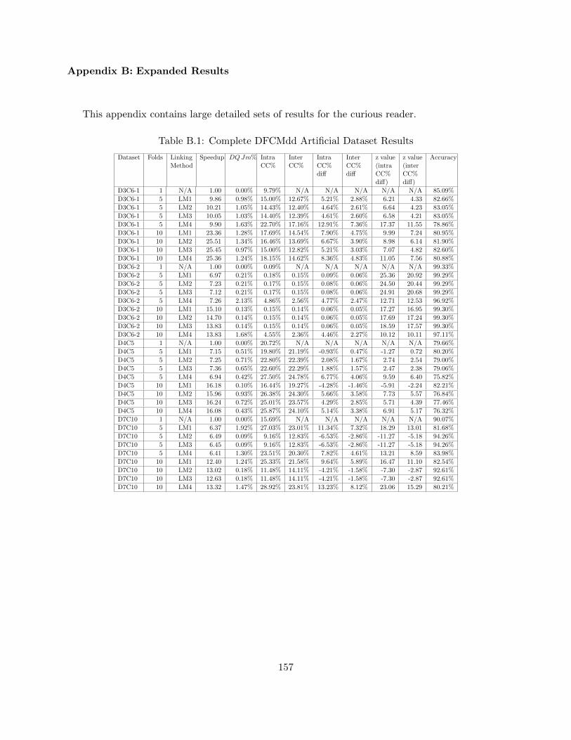
Appendix B: Expanded Results
This appendix contains large detailed sets of results for the curious reader.
Table B.1: Complete DFCMdd Artificial Dataset Results
Dataset Folds LinkingMethod
Speedup DQJm% IntraCC%
InterCC%
IntraCC%diff
InterCC%diff
z value(intraCC%diff)
z value(interCC%diff)
Accuracy
D3C6-1 1 N/A 1.00 0.00% 9.79% N/A N/A N/A N/A N/A 85.09%
D3C6-1 5 LM1 9.86 0.98% 15.00% 12.67% 5.21% 2.88% 6.21 4.33 82.66%
D3C6-1 5 LM2 10.21 1.05% 14.43% 12.40% 4.64% 2.61% 6.64 4.23 83.05%
D3C6-1 5 LM3 10.05 1.03% 14.40% 12.39% 4.61% 2.60% 6.58 4.21 83.05%
D3C6-1 5 LM4 9.90 1.63% 22.70% 17.16% 12.91% 7.36% 17.37 11.55 78.86%
D3C6-1 10 LM1 23.36 1.28% 17.69% 14.54% 7.90% 4.75% 9.99 7.24 80.95%
D3C6-1 10 LM2 25.51 1.34% 16.46% 13.69% 6.67% 3.90% 8.98 6.14 81.90%
D3C6-1 10 LM3 25.45 0.97% 15.00% 12.82% 5.21% 3.03% 7.07 4.82 82.60%
D3C6-1 10 LM4 25.36 1.24% 18.15% 14.62% 8.36% 4.83% 11.05 7.56 80.88%
D3C6-2 1 N/A 1.00 0.00% 0.09% N/A N/A N/A N/A N/A 99.33%
D3C6-2 5 LM1 6.97 0.21% 0.18% 0.15% 0.09% 0.06% 25.36 20.92 99.29%
D3C6-2 5 LM2 7.23 0.21% 0.17% 0.15% 0.08% 0.06% 24.50 20.44 99.29%
D3C6-2 5 LM3 7.12 0.21% 0.17% 0.15% 0.08% 0.06% 24.91 20.68 99.29%
D3C6-2 5 LM4 7.26 2.13% 4.86% 2.56% 4.77% 2.47% 12.71 12.53 96.92%
D3C6-2 10 LM1 15.10 0.13% 0.15% 0.14% 0.06% 0.05% 17.27 16.95 99.30%
D3C6-2 10 LM2 14.70 0.14% 0.15% 0.14% 0.06% 0.05% 17.69 17.24 99.30%
D3C6-2 10 LM3 13.83 0.14% 0.15% 0.14% 0.06% 0.05% 18.59 17.57 99.30%
D3C6-2 10 LM4 13.83 1.68% 4.55% 2.36% 4.46% 2.27% 10.12 10.11 97.11%
D4C5 1 N/A 1.00 0.00% 20.72% N/A N/A N/A N/A N/A 79.66%
D4C5 5 LM1 7.15 0.51% 19.80% 21.19% -0.93% 0.47% -1.27 0.72 80.20%
D4C5 5 LM2 7.25 0.71% 22.80% 22.39% 2.08% 1.67% 2.74 2.54 79.00%
D4C5 5 LM3 7.36 0.65% 22.60% 22.29% 1.88% 1.57% 2.47 2.38 79.06%
D4C5 5 LM4 6.94 0.42% 27.50% 24.78% 6.77% 4.06% 9.59 6.40 75.82%
D4C5 10 LM1 16.18 0.10% 16.44% 19.27% -4.28% -1.46% -5.91 -2.24 82.21%
D4C5 10 LM2 15.96 0.93% 26.38% 24.30% 5.66% 3.58% 7.73 5.57 76.84%
D4C5 10 LM3 16.24 0.72% 25.01% 23.57% 4.29% 2.85% 5.71 4.39 77.46%
D4C5 10 LM4 16.08 0.43% 25.87% 24.10% 5.14% 3.38% 6.91 5.17 76.32%
D7C10 1 N/A 1.00 0.00% 15.69% N/A N/A N/A N/A N/A 90.07%
D7C10 5 LM1 6.37 1.92% 27.03% 23.01% 11.34% 7.32% 18.29 13.01 81.68%
D7C10 5 LM2 6.49 0.09% 9.16% 12.83% -6.53% -2.86% -11.27 -5.18 94.26%
D7C10 5 LM3 6.45 0.09% 9.16% 12.83% -6.53% -2.86% -11.27 -5.18 94.26%
D7C10 5 LM4 6.41 1.30% 23.51% 20.30% 7.82% 4.61% 13.21 8.59 83.98%
D7C10 10 LM1 12.40 1.24% 25.33% 21.58% 9.64% 5.89% 16.47 11.10 82.54%
D7C10 10 LM2 13.02 0.18% 11.48% 14.11% -4.21% -1.58% -7.30 -2.87 92.61%
D7C10 10 LM3 12.63 0.18% 11.48% 14.11% -4.21% -1.58% -7.30 -2.87 92.61%
D7C10 10 LM4 13.32 1.47% 28.92% 23.81% 13.23% 8.12% 23.06 15.29 80.21%
157
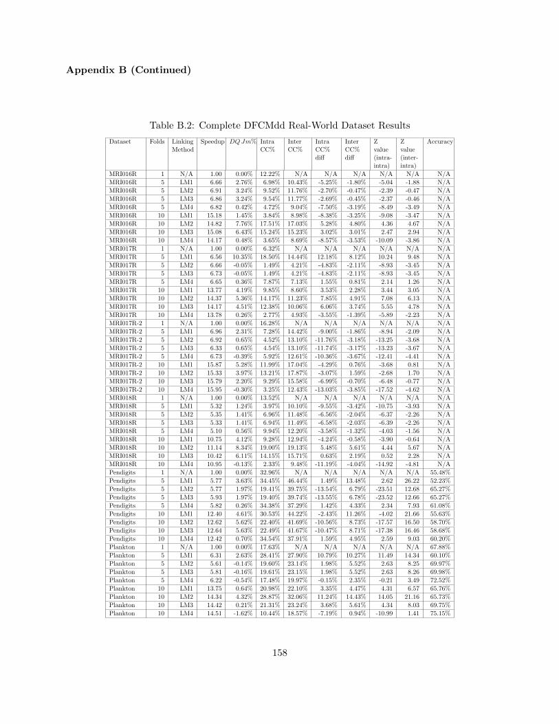
Appendix B (Continued)
Table B.2: Complete DFCMdd Real-World Dataset Results
Dataset Folds LinkingMethod
Speedup DQJm% IntraCC%
InterCC%
IntraCC%diff
InterCC%diff
Zvalue(intra-intra)
Zvalue(inter-intra)
Accuracy
MRI016R 1 N/A 1.00 0.00% 12.22% N/A N/A N/A N/A N/A N/A
MRI016R 5 LM1 6.66 2.76% 6.98% 10.43% -5.25% -1.80% -5.04 -1.88 N/A
MRI016R 5 LM2 6.91 3.24% 9.52% 11.76% -2.70% -0.47% -2.39 -0.47 N/A
MRI016R 5 LM3 6.86 3.24% 9.54% 11.77% -2.69% -0.45% -2.37 -0.46 N/A
MRI016R 5 LM4 6.82 0.42% 4.72% 9.04% -7.50% -3.19% -8.49 -3.49 N/A
MRI016R 10 LM1 15.18 1.45% 3.84% 8.98% -8.38% -3.25% -9.08 -3.47 N/A
MRI016R 10 LM2 14.82 7.76% 17.51% 17.03% 5.28% 4.80% 4.36 4.67 N/A
MRI016R 10 LM3 15.08 6.43% 15.24% 15.23% 3.02% 3.01% 2.47 2.94 N/A
MRI016R 10 LM4 14.17 0.48% 3.65% 8.69% -8.57% -3.53% -10.09 -3.86 N/A
MRI017R 1 N/A 1.00 0.00% 6.32% N/A N/A N/A N/A N/A N/A
MRI017R 5 LM1 6.56 10.35% 18.50% 14.44% 12.18% 8.12% 10.24 9.48 N/A
MRI017R 5 LM2 6.66 -0.05% 1.49% 4.21% -4.83% -2.11% -8.93 -3.45 N/A
MRI017R 5 LM3 6.73 -0.05% 1.49% 4.21% -4.83% -2.11% -8.93 -3.45 N/A
MRI017R 5 LM4 6.65 0.36% 7.87% 7.13% 1.55% 0.81% 2.14 1.26 N/A
MRI017R 10 LM1 13.77 4.19% 9.85% 8.60% 3.53% 2.28% 3.44 3.05 N/A
MRI017R 10 LM2 14.37 5.36% 14.17% 11.23% 7.85% 4.91% 7.08 6.13 N/A
MRI017R 10 LM3 14.17 4.51% 12.38% 10.06% 6.06% 3.74% 5.55 4.78 N/A
MRI017R 10 LM4 13.78 0.26% 2.77% 4.93% -3.55% -1.39% -5.89 -2.23 N/A
MRI017R-2 1 N/A 1.00 0.00% 16.28% N/A N/A N/A N/A N/A N/A
MRI017R-2 5 LM1 6.96 2.31% 7.28% 14.42% -9.00% -1.86% -8.94 -2.09 N/A
MRI017R-2 5 LM2 6.92 0.65% 4.52% 13.10% -11.76% -3.18% -13.25 -3.68 N/A
MRI017R-2 5 LM3 6.33 0.65% 4.54% 13.10% -11.74% -3.17% -13.23 -3.67 N/A
MRI017R-2 5 LM4 6.73 -0.39% 5.92% 12.61% -10.36% -3.67% -12.41 -4.41 N/A
MRI017R-2 10 LM1 15.87 5.28% 11.99% 17.04% -4.29% 0.76% -3.68 0.81 N/A
MRI017R-2 10 LM2 15.33 3.97% 13.21% 17.87% -3.07% 1.59% -2.68 1.70 N/A
MRI017R-2 10 LM3 15.79 2.20% 9.29% 15.58% -6.99% -0.70% -6.48 -0.77 N/A
MRI017R-2 10 LM4 15.95 -0.30% 3.25% 12.43% -13.03% -3.85% -17.52 -4.62 N/A
MRI018R 1 N/A 1.00 0.00% 13.52% N/A N/A N/A N/A N/A N/A
MRI018R 5 LM1 5.32 1.24% 3.97% 10.10% -9.55% -3.42% -10.75 -3.93 N/A
MRI018R 5 LM2 5.35 1.41% 6.96% 11.48% -6.56% -2.04% -6.37 -2.26 N/A
MRI018R 5 LM3 5.33 1.41% 6.94% 11.49% -6.58% -2.03% -6.39 -2.26 N/A
MRI018R 5 LM4 5.10 0.56% 9.94% 12.20% -3.58% -1.32% -4.03 -1.56 N/A
MRI018R 10 LM1 10.75 4.12% 9.28% 12.94% -4.24% -0.58% -3.90 -0.64 N/A
MRI018R 10 LM2 11.14 8.34% 19.00% 19.13% 5.48% 5.61% 4.44 5.67 N/A
MRI018R 10 LM3 10.42 6.11% 14.15% 15.71% 0.63% 2.19% 0.52 2.28 N/A
MRI018R 10 LM4 10.95 -0.13% 2.33% 9.48% -11.19% -4.04% -14.92 -4.81 N/A
Pendigits 1 N/A 1.00 0.00% 32.96% N/A N/A N/A N/A N/A 55.48%
Pendigits 5 LM1 5.77 3.63% 34.45% 46.44% 1.49% 13.48% 2.62 26.22 52.23%
Pendigits 5 LM2 5.77 1.97% 19.41% 39.75% -13.54% 6.79% -23.51 12.68 65.27%
Pendigits 5 LM3 5.93 1.97% 19.40% 39.74% -13.55% 6.78% -23.52 12.66 65.27%
Pendigits 5 LM4 5.82 0.26% 34.38% 37.29% 1.42% 4.33% 2.34 7.93 61.08%
Pendigits 10 LM1 12.40 4.61% 30.53% 44.22% -2.43% 11.26% -4.02 21.66 55.63%
Pendigits 10 LM2 12.62 5.62% 22.40% 41.69% -10.56% 8.73% -17.57 16.50 58.70%
Pendigits 10 LM3 12.64 5.63% 22.49% 41.67% -10.47% 8.71% -17.38 16.46 58.68%
Pendigits 10 LM4 12.42 0.70% 34.54% 37.91% 1.59% 4.95% 2.59 9.03 60.20%
Plankton 1 N/A 1.00 0.00% 17.63% N/A N/A N/A N/A N/A 67.88%
Plankton 5 LM1 6.31 2.63% 28.41% 27.90% 10.79% 10.27% 11.49 14.34 60.10%
Plankton 5 LM2 5.61 -0.14% 19.60% 23.14% 1.98% 5.52% 2.63 8.25 69.97%
Plankton 5 LM3 5.81 -0.16% 19.61% 23.15% 1.98% 5.52% 2.63 8.26 69.98%
Plankton 5 LM4 6.22 -0.54% 17.48% 19.97% -0.15% 2.35% -0.21 3.49 72.52%
Plankton 10 LM1 13.75 0.64% 20.98% 22.10% 3.35% 4.47% 4.31 6.57 65.76%
Plankton 10 LM2 14.34 4.32% 28.87% 32.06% 11.24% 14.43% 14.05 21.16 65.73%
Plankton 10 LM3 14.42 0.21% 21.31% 23.24% 3.68% 5.61% 4.34 8.03 69.75%
Plankton 10 LM4 14.51 -1.62% 10.44% 18.57% -7.19% 0.94% -10.99 1.41 75.15%
158
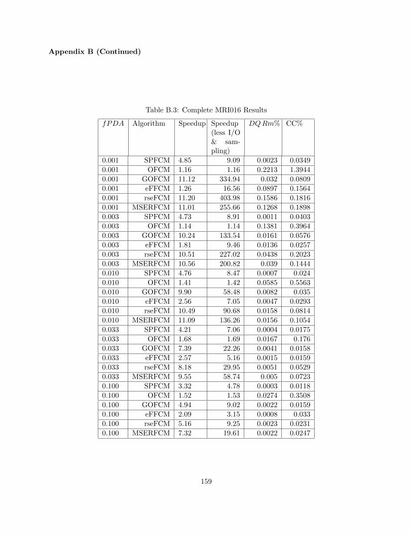
Appendix B (Continued)
Table B.3: Complete MRI016 Results
fPDA Algorithm Speedup Speedup(less I/O& sam-pling)
DQRm% CC%
0.001 SPFCM 4.85 9.09 0.0023 0.0349
0.001 OFCM 1.16 1.16 0.2213 1.3944
0.001 GOFCM 11.12 334.94 0.032 0.0809
0.001 eFFCM 1.26 16.56 0.0897 0.1564
0.001 rseFCM 11.20 403.98 0.1586 0.1816
0.001 MSERFCM 11.01 255.66 0.1268 0.1898
0.003 SPFCM 4.73 8.91 0.0011 0.0403
0.003 OFCM 1.14 1.14 0.1381 0.3964
0.003 GOFCM 10.24 133.54 0.0161 0.0576
0.003 eFFCM 1.81 9.46 0.0136 0.0257
0.003 rseFCM 10.51 227.02 0.0438 0.2023
0.003 MSERFCM 10.56 200.82 0.039 0.1444
0.010 SPFCM 4.76 8.47 0.0007 0.024
0.010 OFCM 1.41 1.42 0.0585 0.5563
0.010 GOFCM 9.90 58.48 0.0082 0.035
0.010 eFFCM 2.56 7.05 0.0047 0.0293
0.010 rseFCM 10.49 90.68 0.0158 0.0814
0.010 MSERFCM 11.09 136.26 0.0156 0.1054
0.033 SPFCM 4.21 7.06 0.0004 0.0175
0.033 OFCM 1.68 1.69 0.0167 0.176
0.033 GOFCM 7.39 22.26 0.0041 0.0158
0.033 eFFCM 2.57 5.16 0.0015 0.0159
0.033 rseFCM 8.18 29.95 0.0051 0.0529
0.033 MSERFCM 9.55 58.74 0.005 0.0723
0.100 SPFCM 3.32 4.78 0.0003 0.0118
0.100 OFCM 1.52 1.53 0.0274 0.3508
0.100 GOFCM 4.94 9.02 0.0022 0.0159
0.100 eFFCM 2.09 3.15 0.0008 0.033
0.100 rseFCM 5.16 9.25 0.0023 0.0231
0.100 MSERFCM 7.32 19.61 0.0022 0.0247
159
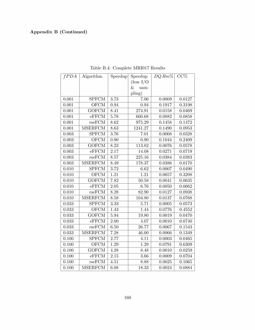
Appendix B (Continued)
Table B.4: Complete MRI017 Results
fPDA Algorithm Speedup Speedup(less I/O& sam-pling)
DQRm% CC%
0.001 SPFCM 3.73 7.06 0.0009 0.0127
0.001 OFCM 0.94 0.94 0.1917 0.3198
0.001 GOFCM 8.41 274.91 0.0158 0.0469
0.001 eFFCM 5.78 660.68 0.0882 0.0858
0.001 rseFCM 8.62 975.29 0.1458 0.1472
0.001 MSERFCM 8.63 1241.27 0.1490 0.0953
0.003 SPFCM 3.76 7.01 0.0008 0.0328
0.003 OFCM 0.90 0.90 0.1044 0.2409
0.003 GOFCM 8.23 113.82 0.0076 0.0578
0.003 eFFCM 2.17 14.08 0.0271 0.0719
0.003 rseFCM 8.57 225.16 0.0384 0.0383
0.003 MSERFCM 8.49 178.37 0.0386 0.0170
0.010 SPFCM 3.72 6.62 0.0007 0.0490
0.010 OFCM 1.21 1.21 0.0657 0.3208
0.010 GOFCM 7.82 50.58 0.0041 0.0635
0.010 eFFCM 2.05 6.76 0.0050 0.0662
0.010 rseFCM 8.28 82.90 0.0127 0.0938
0.010 MSERFCM 8.58 104.80 0.0137 0.0768
0.033 SPFCM 3.33 5.71 0.0005 0.0573
0.033 OFCM 1.43 1.44 0.0776 0.4552
0.033 GOFCM 5.94 19.80 0.0019 0.0470
0.033 eFFCM 2.00 4.07 0.0010 0.0740
0.033 rseFCM 6.50 26.77 0.0067 0.1543
0.033 MSERFCM 7.28 46.00 0.0066 0.1349
0.100 SPFCM 2.77 4.11 0.0003 0.0465
0.100 OFCM 1.29 1.29 0.0791 0.6309
0.100 GOFCM 4.28 8.48 0.0010 0.0259
0.100 eFFCM 2.15 3.66 0.0009 0.0704
0.100 rseFCM 4.51 8.88 0.0025 0.1065
0.100 MSERFCM 6.08 18.33 0.0024 0.0884
160
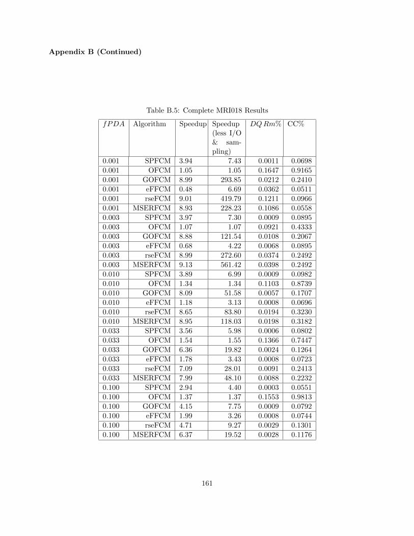
Appendix B (Continued)
Table B.5: Complete MRI018 Results
fPDA Algorithm Speedup Speedup(less I/O& sam-pling)
DQRm% CC%
0.001 SPFCM 3.94 7.43 0.0011 0.0698
0.001 OFCM 1.05 1.05 0.1647 0.9165
0.001 GOFCM 8.99 293.85 0.0212 0.2410
0.001 eFFCM 0.48 6.69 0.0362 0.0511
0.001 rseFCM 9.01 419.79 0.1211 0.0966
0.001 MSERFCM 8.93 228.23 0.1086 0.0558
0.003 SPFCM 3.97 7.30 0.0009 0.0895
0.003 OFCM 1.07 1.07 0.0921 0.4333
0.003 GOFCM 8.88 121.54 0.0108 0.2067
0.003 eFFCM 0.68 4.22 0.0068 0.0895
0.003 rseFCM 8.99 272.60 0.0374 0.2492
0.003 MSERFCM 9.13 561.42 0.0398 0.2492
0.010 SPFCM 3.89 6.99 0.0009 0.0982
0.010 OFCM 1.34 1.34 0.1103 0.8739
0.010 GOFCM 8.09 51.58 0.0057 0.1707
0.010 eFFCM 1.18 3.13 0.0008 0.0696
0.010 rseFCM 8.65 83.80 0.0194 0.3230
0.010 MSERFCM 8.95 118.03 0.0198 0.3182
0.033 SPFCM 3.56 5.98 0.0006 0.0802
0.033 OFCM 1.54 1.55 0.1366 0.7447
0.033 GOFCM 6.36 19.82 0.0024 0.1264
0.033 eFFCM 1.78 3.43 0.0008 0.0723
0.033 rseFCM 7.09 28.01 0.0091 0.2413
0.033 MSERFCM 7.99 48.10 0.0088 0.2232
0.100 SPFCM 2.94 4.40 0.0003 0.0551
0.100 OFCM 1.37 1.37 0.1553 0.9813
0.100 GOFCM 4.15 7.75 0.0009 0.0792
0.100 eFFCM 1.99 3.26 0.0008 0.0744
0.100 rseFCM 4.71 9.27 0.0029 0.1301
0.100 MSERFCM 6.37 19.52 0.0028 0.1176
161