Yohannes yihdego March, 2005
A three dimensional ground water model of the aquifers around Lake Navaisha area, Kenya.
A THREE DIMENSIONAL GROUND WATER MODELLING OF THE AQUIFERS AROUND LAKE NAVAISHA AREA, KENYA
A three-dimensional Ground water model Of the aquifers around
Lake Navaisha area, Kenya
by
Yohannes Yihdego Thesis submitted to the International Institute for Geo-information Science and Earth Observation in partial fulfilment of the requirements for the degree of Master of Science in Geo-information Science and Earth Observation, Specialisation: (Groundwater Resources Evaluation and Management) Thesis Assessment Board Chairman Prof. Dr. Ir. Z. Su External Examiner Drs. J.W.A Foppen (UNESCO -IHE Delft) Primary supervisor Drs.R.Becht Second supervisor Dr. Ing. T.H.M. Rientjes
INTERNATIONAL INSTITUTE FOR GEO-INFORMATION SCIENCE AND EARTH OBSERVATION ENSCHEDE, THE NETHERLANDS
A THREE DIMENSIONAL GROUND WATER MODELLING OF THE AQUIFERS AROUND LAKE NAVAISHA AREA, KENYA
Disclaimer This document describes work undertaken as part of a programme of study at the International Institute for Geo-information Science and Earth Observation. All views and opinions expressed therein remain the sole responsibility of the author, and do not necessarily represent those of the institute.

A THREE DIMENSIONAL GROUND WATER MODELLING OF THE AQUIFERS AROUND LAKE NAVAISHA AREA, KENYA
i
Abstract
Lake Navaisha and aquifer surrounding the lake are important water resources in the area and are used extensively for irrigation and domestic water supplies. Continued or increased withdrawals from these sources have the potential to affect water levels in these aquifers. This thesis presents the design of a 3-D conceptual model of ground-water flow, the development and calibration of a numerical model for steady state groundwater simulation.Part of this study also includes updating the three-dimensional hydro-geologic framework model to serve as the foundation for the development of a steady-state regional ground-water flow model on the basis of integration of geology, hydro-geochemistry, geophysics, isotopic analysis and selection of mathematical boundary conditions. Groundwater flow in the Navaisha basin was modelled numerically with the ground water modelling system(GMS 5.0)and is used to simulate ground-water flow in the aquifers and lake–aquifer interaction. A four layer system was designed from which, the upper two layers represent the sediment aquifer, and the lower layers represent the volcanic aquifer. The regional model area was divided into grid blocks 300 meters areal space while the local and site model have 150m and 80m areal grid spacing respectively. The Navaisha lake is considered as an integral part of the ground water flow system since heads and flow patterns in surficial aquifers can be strongly influenced by the surface Navaisha lake that are are direct contact ,vertically and laterally with the aquifer. The lake was simulated by specifying a high hydraulic conductivity for lake-volume grid cells, the “high K” technique. The model was calibrated to static water level measurements in wells. Pilot points were used as a device for characterisation of parameter spatial variation in conjunction with the regularization in the ground water model calibration. Overall, the finite difference groundwater model result was comparable with measured well data .The simulated head and flow distributions mimic the important aspects of the flow system, such as magnitude and direction of the head contours. Also, simulated lake level varies in a manner determined by the water budget computed for the lake in the model grid. This process is crucial in making the model serve as simulator of the response of lake stage to hydraulic stresses applied to the aquifer and variation in climatic condition, a capability desired by resources manager. The sensitivity of lake level computed using high–K method was tested to the choice of K2/K1, where K1 is the hydraulic conductivity of the lake nodes and K1 is the hydraulic conductivity of the aquifer. The results indicate that values of K2/K1 less than 1000 produced a significant head differential across the lake (computing four wells at the lake surface), which could result in erroneous calculations of seepage to and from the lake. A value of K2/K1 greater than 1000 but less than 1,000,000 gave acceptable solution, produced no gradient across the lake.
A THREE DIMENSIONAL GROUND WATER MODELLING OF THE AQUIFERS AROUND LAKE NAVAISHA AREA, KENYA
ii
Acknowledgements
I appreciate the Netherlands government who sponsored this study through the Netherlands fellowship program. I am grateful to my organization for granting my leave of absence to pursue further studies, and for all the help they have rendered this far. I would like to thank for all WREM staff members .Special thanks go to Arno van lieshout and Robert Becht who made possible for me to switch off to MSc program. The hydro-geological explanations, speculations & all field work with Drs.Robert Becht were quite remarkable. I highly appreciate all the discussions and work I shared with. I do extend similar appreciation to all my colleagues of the Navaisha group. I am indebted to Dr.Tom Rientjes, for his critical comments up to the final write-ups. I do acknowledge all the help of all the other ITC academic and support staff. I do salute the Ethiopian community. I would like to extend my appreciation to Dr. John Doherty (PEST developer, Australia) for his guidance and materials. I am grateful to the GMS forum community (special thanks to Dr.Jeffery, mediator and administrator of GMS, U.S.A) who allowed me to gain and share knowledge from their participation. Last but not least I stretch out my hands to my family and friends for always being there for me.
A THREE DIMENSIONAL GROUND WATER MODELLING OF THE AQUIFERS AROUND LAKE NAVAISHA AREA, KENYA
iii
Dedication
To my father Yihdego Woldeyohannes and my mother Zewdi Asres
To all those who have contributed to my education
A THREE DIMENSIONAL GROUND WATER MODELLING OF THE AQUIFERS AROUND LAKE NAVAISHA AREA, KENYA
iv
Table of contents
Abstract .................................................................................................................................................... i Acknowledgements ................................................................................................................................. ii Table of Content..................................................................................................................................... iv List of Figures ....................................................................................................................................... vii List of Tables ......................................................................................................................................... ix 1. Introduction ....................................................................................................................................11
1.1. Background ...........................................................................................................................11 1.2. Justification...........................................................................................................................11 1.3. Problem statement.................................................................................................................12 1.4. Research question .................................................................................................................12 1.5. Objectives .............................................................................................................................12
General ...........................................................................................................................................12 1.6. The structure of the thesis:....................................................................................................12 1.7. Literature review...................................................................................................................13
2. Description of the study area..........................................................................................................15 2.1. Location ................................................................................................................................15 2.2. Physiography, Landuse and Climate.....................................................................................15 2.3. Hydrology,drainage features and stream flows ....................................................................16 2.4. Geology.................................................................................................................................16 2.5. Hydrogeologic setting...........................................................................................................19
3. Methodological Approach..............................................................................................................22 3.1. Introduction...........................................................................................................................22
3.1.1. Pre-fieldwork activities ....................................................................................................22 3.1.2. Fieldwork..........................................................................................................................22 3.1.3. Post field work..................................................................................................................22
3.2. Frame work for the entire research.......................................................................................22 3.2.1. Pre-field work...................................................................................................................24 3.2.2. Field work.........................................................................................................................24 3.2.3. Post field work..................................................................................................................28 Subsurface characterization ...........................................................................................................28
Convergence of ideas .........................................................................................................................28 3.3. Model ....................................................................................................................................30
3.3.1. Developing conceptual model ..........................................................................................31 3.3.2. Digital elevation model ....................................................................................................32
4. Analysis ..........................................................................................................................................33 4.1. Hydrogeolgical synthesis and groundwater flow analysis....................................................33 4.2. Isotopic analysis....................................................................................................................34 4.3. Hydrogeological setting of the North east Navaisha ............................................................35
4.3.1. Well data analysis.............................................................................................................40 5. Updating the 3D hydrogeological model ......................................................................................44
5.1. Development of Three-Dimensional Hydrogeologic Framework Model.............................46 5.2. Description of the Three-Dimensional Hydrogeologic Framework Model..........................47

A THREE DIMENSIONAL GROUND WATER MODELLING OF THE AQUIFERS AROUND LAKE NAVAISHA AREA, KENYA
v
5.2.1. Sedimentary unit...............................................................................................................48 5.2.2. Volcanic Rocks.................................................................................................................48
5.3. Application of Three-Dimensional Framework Model ........................................................48 5.4. Evaluating the Model............................................................................................................49 5.5. Attribution of Model Cells ...................................................................................................50
6. Conceptual model...........................................................................................................................51 6.1. Potentiometric surface ..........................................................................................................52 6.2. Representation of hydraulic properties.................................................................................52
6.2.1. Interpolation of Structural Surfaces for hydraulic properties ..........................................55 6.3. Recharge ...............................................................................................................................56 6.4. Discharge ..............................................................................................................................60
6.4.1. Evapo-transpiration and Open water evaporation ............................................................60 6.4.2. Well withdrawal ...............................................................................................................60 6.4.3. Seepage outflow ...............................................................................................................62
6.5. Selecting the model boundaries ............................................................................................64 7. Numerical model ............................................................................................................................65
7.1. Model design.........................................................................................................................65 7.1.1. Discretization and Representation of the Hydro-geologic Framework............................65 7.1.2. Boundary condition ..........................................................................................................66
7.2. Initial Conditions ..................................................................................................................68 7.3. Representation of hydraulic properties.................................................................................68 7.4. Representations of recharge and discharge...........................................................................69 7.5. Representation of the lake ....................................................................................................70
8. Model calibration ...........................................................................................................................71 8.1. Automatic Inverse calibration...............................................................................................71
8.1.1. Description of the code PEST ..........................................................................................71 8.1.2. Development of the inverse model...................................................................................72 8.1.3. Inverse calibration results.................................................................................................73 Hydraulic heads and Potentiometric surfaces ................................................................................73 Recharge.........................................................................................................................................76 Hydraulic conductivity...................................................................................................................77 8.1.4. Calibration result evaluation ............................................................................................77
8.2. Sensitivity analysis ...............................................................................................................77 8.3. Regional to local model conversion......................................................................................80
8.3.1. Description of the problem...............................................................................................80 9. Discussion and Conclusion ............................................................................................................82
9.1. Discussion.............................................................................................................................82 9.2. Model limitations..................................................................................................................82 9.3. Conclusion ............................................................................................................................83 9.4. Recommendation ..................................................................................................................84 Supplemental Information.................................................................................................................... i Appendix 1 Geological observation points ........................................................................................ vi Appendix 2. Levelled wells in the study area ................................................................................... vii Appendix 3. Interpretation of well C11527 Geological Log Clearly Indicates existence of two aquifers ............................................................................................................................................. viii
A THREE DIMENSIONAL GROUND WATER MODELLING OF THE AQUIFERS AROUND LAKE NAVAISHA AREA, KENYA
vi
Appendix 4. Pilot point used in conjunction with zonal parameterization for layer 1 ...................... ix Appendix 5. Pilot points used in conjunction with the zonal parameterization for layer....................x Appendix 6 Groundwater flow map for the natural setting prior to 1980(By ower 2000) ................ xi Appendix 7.Pieziometric contour lines as drawn by Githaei(1999).Northern part of the study areaxii Appendix 8.Calculating the General Head Boundary...................................................................... xiii Appendix: 9 Current Piezometric Head Contours. W indicates the depression due to extraction from the well field..................................................................................................................................... xiv Appendix 10. Levelled wells pieziometric data showing the temporal groundwater level ...............xv

A THREE DIMENSIONAL GROUND WATER MODELLING OF THE AQUIFERS AROUND LAKE NAVAISHA AREA, KENYA
vii
List of figures
Figure 2-1.The Location map of the study area .....................................................................................15 Figure 2-2 Geological map of the Nakuru-Navaisha area......................................................................18 Figure 2-3 Pieziometric map of Lake Navaisha & vicinities taken from (Clarke A.C.G. 1990) ...........20 Figure 3-1 Steps undertaken in the study including the process of developing a ground water model.23 Figure 3-2 Location map of Geological observation points together with faults/fractures traced .......26 Figure 3-3.Location of isotope sampled wells .......................................................................................27 Figure 3-4 Topographic and geologic profile along the Navaisha-Elementata basin (Nabidi 2002) ....29 Figure 4-1 view of the study area with geological map and satellite image as a background ...............33 Figure 4-2 Hypothesis 1.H is the Historic heads and C is the current head...........................................36 Figure 4-3 geological interpretation of the 2-D resistivity imaging model section (Tsiboah 2002)......38 Figure 4-4 Hypothetical cross section profile for NE of the study area (with EC value indicated) ......39 Figure 4-5 Hypothesis 3 H is the historic head and C is the current head (Nabidi 2002) .....................40 Figure 4-6 Section showing the groundwater level prior and after to high abstraction times ...............40 Figure 4-7 Ground water elevation map displaying a 3-D view of the cone of depression in 2004 in the well field...........................................................................................................................................41 Figure 4-8 Section along the lake-well fields showing the temporal hydraulic gradient.......................41 Figure 5-1 Section through the solid model ...........................................................................................45 Figure 5-2 cross section from the solid model built using horizon method shown without empty space and overlapping problems ......................................................................................................................45 Figure 5-3 Magnetic anomaly map of Lake Navaisha(Tsiboah 2002)...................................................46 Figure 5-4 Ortho view of the updated solid model ................................................................................49 Figure 5-5 North-south cross section through the central part of the model area..................................49 Figure 6-1 Satellite image draped over the Triangulation Irregular Network (TIN) showing the 3-D view of the study area including subsurface characterization using boreholes to build solid model, done in GMS software. ..........................................................................................................................51 Figure 6-2. A 2D schematic cross section of the conceptual model drawn from the Mau Scarps(western) to the South Kinangop Fault (eastern) through the Lake Naivasha basin. Not drawn to scale....................................................................................................................................................52 Figure 6-3 Fractures/faults shown on the geological map (The white colors are Lake Navaisha at center and Lake Elementata at the Northern margin) ............................................................................56 Figure 6-4 Analytical signal image of the study area (Tsiboah 2002)...................................................63 Figure 7-1 Deformed layer approach discretization (honors the stratigraphy of the area) ....................66 Figure 7-2 wells (and springs) heads used for assigning specific head nodes. .....................................67 Figure 7-3 Zonation of horizontal hydraulic conductivity of the sediment aquifer...............................68 Figure 7-4 Zonation of hydraulic conductivity of the volcanic aquifer. ................................................69 Figure 7-5 Zonation of recharge.............................................................................................................69 Figure 7-6 Cross-sectional view of a lake showing its volumetric budget components ........................70 Figure 8-1 Spatial location Pilot points used to estimate the hydraulic conductivities of layer 1(right) and layer 2(left) ......................................................................................................................................72 Figure 8-2 Computed versus observed head value for the selected observation wells ..........................73 Figure 8-3 Simulated groundwater flow in the layer1 (lake sediment aquifer) .....................................75 Figure 8-4 Simulated contour map of the volcanic aquifer for the steady-state simulation (layer4).....76

A THREE DIMENSIONAL GROUND WATER MODELLING OF THE AQUIFERS AROUND LAKE NAVAISHA AREA, KENYA
viii
Figure 8-5 Effect of regional gradient and value of K2/K1 on the calculated hydraulic gradient across the lake ...................................................................................................................................................79 Figure 8-6 Local model ..........................................................................................................................81 Figure 8-7 Site model (well field area) ..................................................................................................81
A THREE DIMENSIONAL GROUND WATER MODELLING OF THE AQUIFERS AROUND LAKE NAVAISHA AREA, KENYA
ix
List of tables
Table 2-1 Summary of geological succession in the study area ............................................................17 Table 3-1 Summary of Lake Elementata water balance.........................................................................29 Table 4-1 Isotope analysis result............................................................................................................34 Table 4-2 The percentage of lake water in boreholes ............................................................................35 Table 4-3 Navaisha basin water budget(After : LNROA 1996:(GoldsonJohn 1993)...........................42 Table 5-1. The lithiological units making up the hydro geological units in the study area...................47 Table 6-1 Average aquifer characteristics of the selected areas and lithiologies from borehole data(figures in brackets are geometric means),(Clarke A.C.G. 1990) ...................................................53 Table 6-2 Transmissivity of different volcanic rocks in various parts of the world (Singhal 1997).....53 Table 6-3 Summary of aquifer properties ..............................................................................................54 Table 6-4 previously published hydraulic properties within or near the study area..............................54 Table 6-5 Direct recharge estimate from SWAP model (1990-1997), before El Nino, by (Nalugya 2003) ......................................................................................................................................................57 Table 6-6 Direct recharge estimate from SWAP model (1997-1998), after El Niño, by (Nalugya 2003)................................................................................................................................................................57 Table 6-7 Apparent recharge estimated by (Mcann 1974).....................................................................59 Table 6-8 Ground water abstraction: Lake Naivasha Basin Estimates (Aquasearch 2001) ..................61 Table 6-9 Estimated abstraction rates for wells completed in the lake sediment (1979-2004) .............62 Table 8-1 A lists of observed and simulated heads together with their differences for the selected wells .......................................................................................................................................................74 Table 8-2 Results for the simulation ......................................................................................................78 Table 9-1 Suggested monitoring wells...................................................................................................85

A THREE DIMENSIONAL GROUND WATER MODEL OF THE AQUIFERS AROUND LAKE NAVAISHA AREA, KENYA
11
1. Introduction
1.1. Background
Lake Navaisha is the only freshwater resources among many saline lakes in the Kenyan rift valley. Several studies have been carried out in Lake Navaisha area to increase the knowledge of the groundwater system, lake-aquifer interaction and accomplish a proper management of their resources. Quantitative Solutions in Hydrogeology and Groundwater Modeling addresses and solves a variety of questions and problems from hydro-geological practice(Kresic 1997). In recent years, the simulative capabilities of ground-water flow models have been enhanced by the development of increasingly sophisticated methods of representing the effects of external hydraulic influences on heads and flow patterns in ground-water systems. Heads in surficial aquifers, in particular, can be strongly affected by the hydraulic influence of bodies of surface water and by exchanges of water volumes with the overlying atmosphere. One particular example is the influence of surface water, such as lakes, that are in direct contact, vertically and laterally, with the surficial aquifer. The magnitudes of significant terms (sources and sinks) in the water budgets of lakes commonly differ from corresponding terms of water budgets of adjacent surficial aquifers, so that varying hydrologic conditions can cause either the lake or the aquifer to affect the head in the other water body. In regions with economically important lakes like Lake Navaisha, it is helpful to have an available technique to describe the hydraulic interaction between a lake and the surrounding aquifer so that the effect of changes in either water body on conditions in the other can be estimated by resource managers. Future success in understanding the dynamic nature of the groundwater system of the basin will rely on continued and expanded data collection at various scales, improved methods for quantifying heterogeneity in subsurface hydraulic properties, enhanced modelling tools and understanding of model uncertainty, and greater understanding of the role of climate and interactions with surface water.
1.2. Justification
The need to rely upon model of the hydro-geological system of Lake Navaisha area helps: • To understand and predict a ground water flow system .It allows for better understanding of
the ground water flow and predicting future impacts on ground water quantity and quality of the study area.
• To simulate hypothetical situation of the flow system to gain insight in it.
Numerical simulation is best way to test hypothesis and integrate the various pieces. Simulation is powerful tool for analysis because it accounts all physical and chemical process simultaneously as in nature. Thus it helps to gain insight and understanding rather than for predictive purposes. In many cases simplification provides adequate simulation. However it is important to recognize that in area where fracture flow is evident is the groundwater flow is 3-D in nature. Thus, development of 3D hydro-geologic models for the lake Navaisha is necessary to improve our understanding of ground

A THREE DIMENSIONAL GROUND WATER MODEL OF THE AQUIFERS AROUND LAKE NAVAISHA AREA, KENYA
12
water flow pattern. Improved understanding of the hydrogeology framework is needed to address the significance of ground water to Lake Navaisha and its water balance. Two major steps were necessary to complete the study: 1. Detailed hydrogeology characterization 2. The development of numerical ground water flow model. The focus of this study is to develop three-dimensional ground-water flow model that contributes to a better understanding of the lake- aquifer system using 3-D hydro-geological model as a basis.
1.3. Problem statement
In Lake Navaisha area context a ground water flow model would essentially be in class of complex numerical model due to the complexity of the hydro-geological system. The understanding of the flow system of this area has been approached principally using Piezometric level as determinant for the ground water flow pattern and hydrogeology has been considered (handled two dimensionally) in few studies like (Kibona 2000) disregarding vertical flow and possibilities of multiple aquifers. Development of the three-dimensional model was initiated to address several of the assumptions described by previous researchers.
1.4. Research question
Will the 3-D conceptual hydro-geological model provides the geometric framework into which the available hydro-geological data can be hung and the groundwater flow patterns can be postulated?
1.5. Objectives
General
The main objective is to improve the knowledge of the complex hydrodynamics of the Naviasha Lake –aquifer system by consolidating all the previous works on groundwater modelling.
Specific objective
1. Updating the 3-D hydro-geological conceptual model for the Navaisha area and link to the adjacent Elementata and Nakuru basin 2. Discretize the study area into a three-dimensional finite-difference grid 3. Set-up the model
1.6. The structure of the thesis:
This thesis consists of nine chapters followed by different appendixes to which references are given through the text. Chapter 1: introduction of the research. It includes the importance of the research, the problem and the objectives of the research are described followed by research questions. Previous works related to the subject is dealt with in this chapter. Chapter2: Description of the study area. An overview of different aspects that characterize the project area is given here. Given the enormous amount of work already done in the area, this chapter has been adapted from the work of (Ower 2000) and (Nabidi 2002) Chapter3: Methodological Approach is presented in this chapter. It outlines the stages and approaches involved, right from the preparations before fieldwork until the completion of the project.
A THREE DIMENSIONAL GROUND WATER MODEL OF THE AQUIFERS AROUND LAKE NAVAISHA AREA, KENYA
13
Chapter 4: Analysis data collected from the field work and also from the previous works were analyzed. Chapter 5: Updating the 3-D Hydro-geological model. This discusses about the development of hydro-geological frame work up to evaluation of the model. Chapter 6: Developing conceptual model. A conceptual model was developed using GMS supported by map and GIS modules to define boundary condition, assigning recharge, hydraulic and to characterize feature coverage’s for MODFLOW. Chapter 7: Numerical modelling. Using the3-D hydro-geological frame model as a basis for the numerical model. Chapter 8: Model calibration with trail and error and automatic inverse modelling. The results from the analysis. Chapter 9: Conclusions and Recommendations. It incorporates the conclusions and recommendations for further studies including limitations .This chapter is concluded by appropriate recommendations in relation to the study objectives based on the answers to the research question.
1.7. Literature review
Many works have been done to improve our understanding of groundwater resources in the Lake Navaisha area. An important activity has been carried out in the development of groundwater model. At the beginning the model effort was primarily geared towards testing ideas about how the system behaves than for predictive purpose.(Trottman 1997)exercised preliminary ground water model to investigate the hydraulic interaction between Lake Navaisha and the surrounding unconfined aquifer and to study the changes in ground water storage of the aquifer in response to fluctuating lake levels. However many assumptions and generalization were made in calculating the model inputs which oversimplified the complex aquifer system of this area. (Baher 1997)Tried to improve the knowledge of the interaction between the lake Navaisha and the surrounding aquifers. He used a cross sectional model to study the interaction between the lake and ground water and to study ground water storage by optimizing different aquifer parameters like transmissivity and storage coefficient, which are used to quantify the change the storage change.(Baher 1997)also investigated the ground water storage behavior of the aquifer in relation to the lake level and to quantify the contribution of ground water as a potential water resource with scarce aquifer parameters and inaccurate boundary conditions. A ground water model has developed and calibrated to estimate the amount of flow from Malawa River to the well field as well as from Lake Navaisha by(Hermandez 1999) One of the positive remarks is the model results was evaluated from an environmental point of view. However the validity of the model could not be assured due to scarcity of observations. A number of numerical models have been developed to estimate the long-term water balance of the lake-aquifer systems of the Navaisha Basin. Numerical models used to quantify the water exchange between a lake and groundwater typically use a constant head condition to represent the average level of the lake. However, lake levels often show long and short-term transience. Precipitation to and evaporation from the Lake Surface, stream flow, and groundwater fluxes have to be considered. These flow components affect lake levels and changes in them lead to lake level fluctuations(Cheng. 1993) . The flow from Lake Navaisha is directed more to the south than to the north this is supported by the proportion of groundwater deficit of the neighbouring lakes though not conclusive, further it is supported by groundwater level as manifested on the piezometry and isotopic evidence (Muno2002). Groundwater isotope provided useful information though more in a qualitative sense supporting the hypothesis that larger proportion of lake water flows more to the south than to the north.
A THREE DIMENSIONAL GROUND WATER MODEL OF THE AQUIFERS AROUND LAKE NAVAISHA AREA, KENYA
14
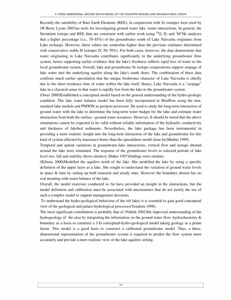
Recently the suitability of Rare Earth Elements (REE), in conjunction with Sr isotopes were used by (W.Berry Lyons 2003)as tools for investigating ground water lake -water interactions. In general, the Strontium isotope and REE data are consistent with earlier work using 18O, D, and 3H/3He analyses that a higher percentage (i.e., 70–85%) of the groundwater south of Lake Naivasha originates from Lake recharge. However, these values are somewhat higher than the previous estimates determined with conservative stable H isotopes D, 50–70%). For both cases, however, the data demonstrate that water originating in Lake Naivasha contributes significantly to the underlying groundwater flow system, hence supporting earlier evidence that the lake's freshness reflects rapid loss of water to the local groundwater system. Overall, lake and groundwater Sr isotope compositions support seepage of lake water into the underlying aquifer along the lake's south shore. The combination of these data confirms much earlier speculation that the unique freshwater character of Lake Naivasha is chiefly due to the short residence time of water within the lake itself. Hence, Lake Naivasha is a "seepage" lake in a classical sense in that water is rapidly lost from the lake to the groundwater system (Ower 2000)Established a conceptual model based on the general understanding of the hydro-geologic condition .The lake water balance model has been fully incorporated in Modflow using the non-standard lake module and PMWIN as pre/post processor. He used to study the long-term interaction of ground water with the lake to determine the long-term water budget for the lake and estimate water abstraction from both the surface –ground water resources. However, It should be noted that the above simulations cannot be expected to be valid without reliable information of the hydraulic conductivity and thickness of lakebed sediments. Nevertheless, the lake package has been instrumental in providing a more realistic insight into the long-term interaction of the lake and groundwater for this kind of system affected by transience better than the spreadsheet model done by(Mmbui 1999) Temporal and spatial variations in groundwater-lake interactions, vertical flow and storage abound around the lake were simulated. The response of the groundwater levels to selected periods of lake level rise, fall and stability shows mimicry (Baher 1997)findings were similar). (Kibona 2000)Modelled the aquifers north of the lake .She modelled the lake by using a specific definition of the upper layer as a lake. She sought to understand the variation of ground water levels in space & time by setting up both transient and steady state. However the boundary chosen has no real meaning with water balance of the lake. Overall, the model exercises conducted so far have provided an insight in the interactions, but the model definition and calibration must be associated with uncertainties that do not justify the use of such a complex model to support management decisions. To understand the hydro-geological behaviour of the rift lakes it is essential to gain good conceptual view of the geological and palaeo-hydrological processes(Tenalem 1998). The most significant contribution is probably that of (Nabidi 2002)He improved understanding of the hydrogeology of the area by integrating the information on the ground water flow, hydrochemistry & boundary as a basis to construct a 3-D conceptual-hydro-geological model taking geology as a prime factor. This model is a good basis to construct a calibrated groundwater model. Thus, a three-dimensional representation of the groundwater system is required to predict the flow system more accurately and provide a more realistic view of the lake-aquifers setting.

A THREE DIMENSIONAL GROUND WATER MODEL OF THE AQUIFERS AROUND LAKE NAVAISHA AREA, KENYA
15
2. Description of the study area
2.1. Location
The study area is situated in the East Kenyan rift valley province in Nakuru District, about 100 km northwest of Nairobi. It is located in the central rift valley of Kenya between latitudes 00 10’S to 10 00’S and longitudes 36 0 10’E to 36 0 45’E, with UTM zone 37 south and covers an area of about 3500km2 .
Figure 2-1.The Location map of the study area
2.2. Physiography, Landuse and Climate
Lake Naivasha dominates the central part of the Navaisha basin. It has a mean surface area of 145 km2 at an average altitude of 1887.3 m.a.m.s.l (Mmbui 1999)The Mau escarpment on the western fringe rises up to a maximum of 3080 m.a.m.s.l with a N-NNW orientation. The escarpment is rugged and deeply incised with numerous faults and scarps that are prevalent. To the east is the broad Kinangop plateau that rises to a maximum altitude of 2740 m.The NNW- trending south Kinanagop fault scarp (100-240m;(Clarke A.C.G. 1990)separates the plateau from the plain in a series of down throw fault steps. The principal land use is agriculture which includes crop farming (horticulture, vegetables and fruits) around the lake and a mixing farming on the rainfed slopes of the escarpment. The Eburru hills, Mau,

A THREE DIMENSIONAL GROUND WATER MODEL OF THE AQUIFERS AROUND LAKE NAVAISHA AREA, KENYA
16
and Longonot escarpments are all hosts to indigenous hard wood forests that form the main water shed of the lake basin. The basin lies with in the semi-arid belt of Kenya with average annual precipitation of 700m (Ewbank Preece Ltd, 1990).The rainfall pattern is bimodal with the main rainy period in April-may and the shorter one from October-November. It is greater along the Mau and Aberare escarpments where it averages from 1250-1500 mm annually and is lower in valley areas where it averages about 650 mm at lake Navaisha being noticeably as a function of topography. There is an annual potential evaporation estimated at about 1700 mm(Mcann 1974).Monthly averaged potential evaporation on the floor of the basin exceeds rainfall by a factor of 2 to 8 for every month except April when the potential evaporation still exceeds rainfall for the wettest years. Mean daily temperatures vary between 9 oc at night to 25 oc during the day.
2.3. Hydrology,drainage features and stream flows
The Naviasha catchment is separated from the Nakuru-Elementata catchments by the Eburru Volcanic pile which is linked to the Mau Escarpment by a ridge at an altitude of around 2600m.a.m.s.l between the Eburru and Bahati Escarpment the surface drainage divide runs via Gilgil along a culmination of the rift floor at an altitude of approximately 2000 m.a.m.a.s.l.To the south of lake Navaisha the surface water divide runs from the Mau escarpment in the west ,via the Olkaria and Longonot to the Kinangop plateau . Lake Naviasha occupies the bottom of the rift valley and is in the middle of three major centeres of geothermal activity:the Eburru hills to the northwest,Mt Longonot to the southeast,and Olkaria to the south.The lake is the highest and freshest of all the lakes in the rift valley system.The lake level has been fluctuating thus affecting its area and volume and gradually declining over time. The major streams that drain the study area are the Malewa River and the Gilgil River. Ground-water discharge from the weathered volcanic aquifers provides base flow to the Rivers. The Malewa river is one of the two main perennial rivers that drain the lake and flow in a graben at the foot of the kinanagop plateau. The Malewa and Turesha rivers have a combined drainage area of about 1,730 km2.The Kinanagop rivers are captured by the main Malewa river in the north east of the basin. Further downstream the Malewa river is joined by the Turash a river and the two flows south wards. The Gilgil river flows in a narrow basin to the north of the basin and is the second major perennial river that drains the lake..
2.4. Geology
The tectonic and volcanic regimes that led to the formation of the Kenya Rift commenced in the early to mid-Miocene. The geology of the Navaisha basin is a succession of late teritiary and quaternary volcanics with inter-leafing lacustrine beds and alluvium of reworked volcanic debris. The volcanic rocksintheareaconsistofTephrites,basalts,trachytes,phonloites,ashes,tuffs,agglomeratesandacidiclavas(rhyolite,pumice,comendite and obsidian).The lake beds are mainly composed of reworked volcanic material .Despite their extensive distribution the exposed lakebeds are not thick and rarely 30 m.The structure of the area comprise faulting on the flanks and in the floor of the rift valley. Slight unconformities are present in the lake beds and can mostly seen along the Malewa river drainage.
A THREE DIMENSIONAL GROUND WATER MODEL OF THE AQUIFERS AROUND LAKE NAVAISHA AREA, KENYA
17
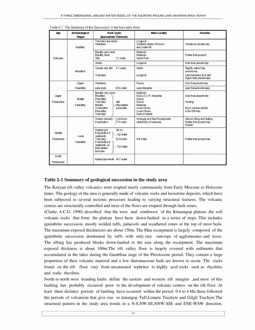
Table 2-1 Summary of geological succession in the study area The Kenyan rift valley volcanics were erupted nearly continuously from Early Miocene to Holocene times. The geology of the area is generally made of volcanic rocks and lacustrine deposits, which have been subjected to several tectonic processes leading to varying structural features. The volcanic centres are structurally controlled and most of the flows are erupted through fault zones. (Clarke A.C.G. 1990) described that the west and southwest of the Kinanagop plateau ,the soft volcanic rocks that form the plateau have been down-faulted in a series of steps. This includes ignimbrite succession, mostly welded tuffs, palaesols and weathered zones at the top of most beds. The maximum exposed thicknesses are about 150m. The Mau escarpment is largely composed of the ignimbrite succession dominated by tuffs with only rare outcrops of agglomerates and lavas. The rifting has produced blocks down-faulted to the east along the escarpment. The maximum exposed thickness is about 100m.The rift valley floor is largely covered with sediments that accumulated in the lakes during the Gamblian stage of the Pleistocene period. They contain a large proportion of their volcanic material and a few diatomaceous beds are known to occur. The rocks found on the rift floor vary from unsaturated tephrites to highly acid rocks such as rhyolites and sodic rhyolites. North to north west trending faults define the eastern and western rift margins ,and most of this faulting has probably occurred prior to the development of volcanic centres on the rift floor. At least three distinict periods of faulting have occurred within the period 0.4 to 4 Ma these followed the periods of volcanism that give rise to kinangop Tuff,Limuru Trachyte and Gilgil Trachyte.The structural pattern in the study area trends in a N-S,NW-SE,NNW-SSE and ENE-WSW direction.

A THREE DIMENSIONAL GROUND WATER MODEL OF THE AQUIFERS AROUND LAKE NAVAISHA AREA, KENYA
18
Faults and fractures are common in the western part compared to the eastern part where large volumes of pyroclastic deposits are present. The younger N-S faults and fractures are common in the axial region of the rift and represent the latest volcanic activity. Vertical permeability along some of these faults is indicated by the occurrence of strong fumarilic activity.The NW-SE trending faults are mostly inferred from aerial photos and alignment of volcanic centres.The Mau escarpment prominently displays the NNW-SSE angle fault trend. The ENE-WSW trending fault s called Olkaria fault zones cuts through the geothermal area and are the most important permeable structures in the whole Olkaria geothermal area.
Figure 2-2 Geological map of the Nakuru-Navaisha area

A THREE DIMENSIONAL GROUND WATER MODEL OF THE AQUIFERS AROUND LAKE NAVAISHA AREA, KENYA
19
2.5. Hydrogeologic setting
The lake Navaisha catchment is hydro-geologically complex due to the rift valley geometry and tectonics(Clarke A.C.G. 1990)The main aquifer is found in sediments covering parts of the rift floor. Ground water is encountered at depths of 3-35m below ground level in the lake bed aquifer, which is usually semi-confined. These aquifers usually have relatively high permeability and are often unconfined with high specific yield(Stuttard 1995).(Clarke A.C.G. 1990)noted that also aquifers are normally found in fractured volcanics or along weathered contacts between different lithiological units.These aquifers are often confined or semi confined and storage coefficients are likely to be low. Aquifers with high permeability are found in sediments covering areas around the lake. They are often unconfined and will have relatively high specific yields.This is in agreement with (Mcann 1974); (Ojiambo 1992)who also noted that the wells near the lake Navaisha shore yield water from lacustrine deposit aquifers and usually have higher specific discharge and transmissivities than wells further away from the lake Most of the production wells in the Olkaria reservoir are from fractured trachytes and basalts and from contacts between these lavas and pyroclasts(Ojiambo 1992). Groundwater in the area is variable in quality both spatially and temporally, for reason still unclear. Records(ground water survey,Kenya,1989) show that water from lake foreshore boreholes are poor in quality with an EC range of 1430-45550 µs/cm.Some boreholes in the inland lake beds have changed in quality after years of pumping, but the majority at the time of drilling were mildy to moderate alkaline and of sodium-bicarbonate type with EC in the range of 300-1490 µs/cm(Aqua-search 2001) Ground water occurrence is greatly determined by the geological conditions as well as the available water for storage. The high hydraulic gradient accounts for the outflow of groundwater from the lake to the south as well as some infinitesimal outflow towards the north. Structural features such as faults often optimize storage, transmissivity and recharge with the significant of these occurring in places that are adjacent to or within a surface drainage system. Tectonic movements of the rift valley have important effects on the aquifer properties both on a small scale by creating the local fracture systems which comprises many aquifers and on a large scale by forming regional hydraulic barriers or shatter zones of enhanced permeability. Clark Et al .,1995 noted that the area has complex hydrogeology ,because while it is lower than rift escarpments it is at culmination of the rift floor. Flow towards lake Navaisha from the Mau escarpment and the Kinangop plateau is unambiguous and some of the ground water from the western side of the rift must eventually form parts of the discharges at Olkaria andEburru.However the longitudinal flows in this area are more difficult to assess. The piezomtric surface has an uninterrupted fall from lake Navaisha, around the east side of Eburru ,towards lake Elemenata ,indicating flow in this direction. It is probable that while shallow ground waters on the south side of Eburru move locally towards Naivasha,deeper flows are substantially north and south wards.
A THREE DIMENSIONAL GROUND WATER MODEL OF THE AQUIFERS AROUND LAKE NAVAISHA AREA, KENYA
20
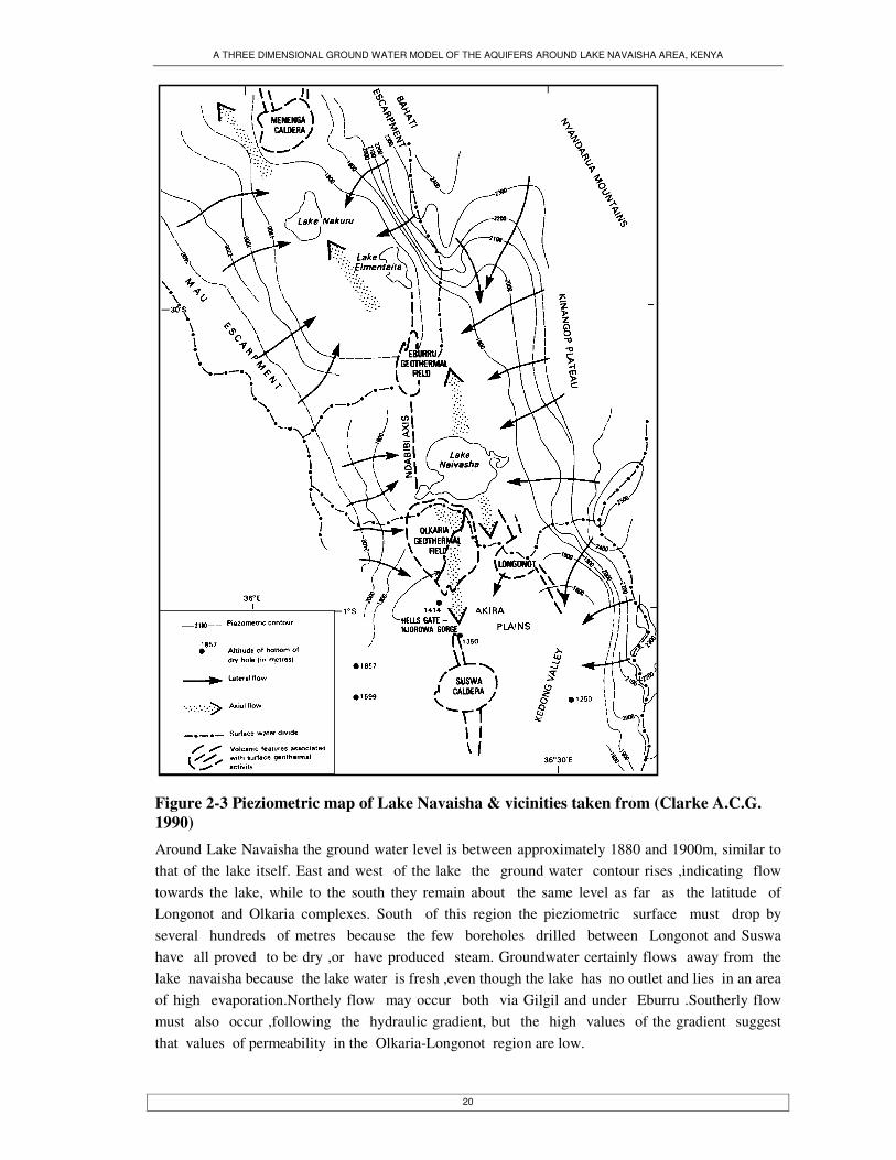
Figure 2-3 Pieziometric map of Lake Navaisha & vicinities taken from (Clarke A.C.G. 1990) Around Lake Navaisha the ground water level is between approximately 1880 and 1900m, similar to that of the lake itself. East and west of the lake the ground water contour rises ,indicating flow towards the lake, while to the south they remain about the same level as far as the latitude of Longonot and Olkaria complexes. South of this region the pieziometric surface must drop by several hundreds of metres because the few boreholes drilled between Longonot and Suswa have all proved to be dry ,or have produced steam. Groundwater certainly flows away from the lake navaisha because the lake water is fresh ,even though the lake has no outlet and lies in an area of high evaporation.Northely flow may occur both via Gilgil and under Eburru .Southerly flow must also occur ,following the hydraulic gradient, but the high values of the gradient suggest that values of permeability in the Olkaria-Longonot region are low.

A THREE DIMENSIONAL GROUND WATER MODEL OF THE AQUIFERS AROUND LAKE NAVAISHA AREA, KENYA
21
(Mcann 1974)in the hydro-geological study of ground water level changes in the Navaisha catchments noted that seasonal water level changes ranged from 0.5 to 0.25 m in response to ground water recharges. Changes were greater in the high land areas and less in lowland areas surrounding lake Navaisha. Annual water level changes were less than 0.2 m that was probably related to below normal rainfall rather than the effects of ground water extractions from water wells. Clark Et al.,1995 found that in the majority of wells only a yield and pumped water levels at equilibrium have been noted only in few cases have recovery data recorded .the highest values of permeability are found in reworked volcanics composing the sediments of Navaisha area, where the specific capacities of wells often exceeds 3 l/s/m and where estimated hydraulic conductivities of greater than 10 m/d are common.On the rift escarpments, the permeabilties of different rocks types are uniformly low. Mean borehole specific capacities and estimated hydraulic conductivities range from 0.21l/s/m and 0.1 m/d for the Kinanagop Tuff to 0.2221 l/s/m and 1.1m/d for the limuru trachyte to the east of Suswa and the Mau tuff. (Clarke A.C.G. 1990) estimated by inventory of boreholes and envisaged that the lake sediments have high permeability of 12-148m/d. The structure of the rift valley, in particular major marginal rift faults , the system of grid faulting and the rift floor undoubtly have substantial effect on the ground water flow systems of the area. In general faults are considered to have two effects on fluid flow. They may facilitate flow by providing channels of high permeability ,or they may prove to be barriers to flow by offsetting zones of relatively high permeability. In the rift valley the main direction of faulting is along the axis of the rift ,and this has a significant effect on the flows across the rift. It is apparent from the high hydraulic gradients that are developed across the rift escarpments that the effects of the major fault is to act as zones of low permeability. The effect of faulting is to cause ground water flows from the sides of the rift towards the centre to flow longer paths reaching greater depths, and to align flows with in the rift along its axis as shown in figure 3 above.(Mcann 1974) noted that the intense faulting between Lake Navaisha and the Kinanagop plateau also appeared to control the movement of ground water in the south east part of the Navaisha catchment.(Clarke A.C.G. 1990)used stable isotope technique to show that lake water appeared to be detectable at least 30 km to the south at the Suswa volcano. They showed that the reservoir fluid could be explained by a 2:1 mixture of lake water with unmodified meteoric recharge from the rift wall area. Isotopic evidence from the Eburru well shows that the lake water passes beneath the Eburru volcanic ridge( Clarke Darling Et al .,1996).Piezomtric plots and isotopic studies show that underground movement of water is occurring both axially along the rift and laterally from the bordering highlands in to the rift .(Nabidi 2002) concluded that the smaller faults on the eastern and western escarpment impede the flow of water from the escarpment to the lake which agrees with figure 2-3 above. Along the rift floor; however, these faults constitute preferential flow paths of outflow.

A THREE DIMENSIONAL GROUND WATER MODEL OF THE AQUIFERS AROUND LAKE NAVAISHA AREA, KENYA
22
3. Methodological Approach
3.1. Introduction
The methodology followed in this study was based on the objectives of the study as stated in section 1.4. In this chapter, the lay out of the key stages and the activities under them are presented. Besides, the major sources of information and materials used are stated.
3.1.1. Pre-fieldwork activities
Literature review of the work done already in the area Data mining for and processing of already available data. Integrating and revising the isotopic, chemical, geological, hydro-geological, hydrological and geophysical analysis and interpretation Acquisition of equipment for field work
3.1.2. Fieldwork
Collection of water sample for isotopic analysis Description of geological observation points Collection of recently drilled boreholes Levelling of wells to define the ground water flow gradient in the vicinity of Lake Navaisha area
3.1.3. Post field work
Data processing and analysis Update the 3D conceptual hydro-geological model of the aquifer system in place Subsurface characterization of the area using horizon-solid method. Developing conceptual model in GMS software using Map and GIS module to characterize the feature coverage’s, boundary, input parameters, sinks and sources. Developing and calibrating the numerical model using manual and automatic (PEST) using pilot points and regularization for model parameterization .The pilot point was used as a device for characterization of parameter spatial variation in the lake sediment aquifer. Zonation was used for parameterization together with pilot points.
3.2. Frame work for the entire research
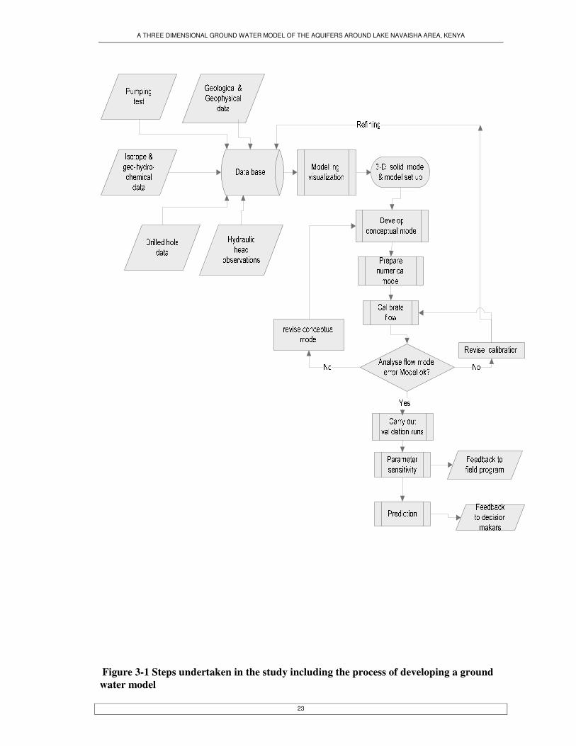
The modelling effort may be divided in to four stages: the compilation of the data, the development of a conceptual model, the calibration of the model, and the application of the model. The schematic representation of the breakdown and sequence of the study process is shown in Figure 3.1
A THREE DIMENSIONAL GROUND WATER MODEL OF THE AQUIFERS AROUND LAKE NAVAISHA AREA, KENYA
23
Figure 3-1 Steps undertaken in the study including the process of developing a ground water model

A THREE DIMENSIONAL GROUND WATER MODEL OF THE AQUIFERS AROUND LAKE NAVAISHA AREA, KENYA
24
3.2.1. Pre-field work
In the preliminary stages of the study a literature review and preparation for field work was carried out. The existing well database was updated and reorganized. Available delineated and appropriate field materials and tools identified. The following materials were used
Topographic maps
Naivasha sheet 133/2, 1975, Longonot sheet 133/4, 1975, Nakuru, sheet 119/3 1975, Gilgil, sheet 119/4, 1975, (UK Ordnance survey overseas survey Department maps, scale 1:50,000)
Geological maps
Geologic map of Longonot Volcano, the greater Olkaria and Eburru volcanic complexes and adjacent areas,1988, 1:100,000,Government of Kenya,Minstry of Energy Geothermal section. Satellite Images Landsat TM images (band 3, 4, 5), 21 January 2003(western part) and 25 February 2003(eastern part)
Groundwater well records
Borehole pumping tests data Well completion records, Well water level monitoring data
References
A number of research papers ,MSc thesis, consultant papers,manscripts,and journal articles from past works in the lake Navaisha basin were used in this study(see references).
Equipments
The following equipment and materials were used in the field: Water level current meter Geological compass (to measure dip and strike of rock formations and faults/fractures) Field geological equipment including geological hammer, magnifier and Garmin GPS Besides the key sources of information Drillers logs for boreholes in Nakuru district Ground water analysis of boreholes and wells from Ministry of land Reclamation, Regional and water Development water resources division, Nairobi 1941-2004 Isotope data analysis by (Oppong-Boateng 2001) Isotope data analysis of Lake Navaisha, geothermal well and boreholes by the British geological survey Isotope data analysis by (Ojiambo 1992; Ojiambo 1996) Isotope data analysis by (Bwire Ojiambo, Berry Lyons et al. 2003) Recharge estimation by (Nalugya 2003) Landsat images: bands 7 taken Sep 9 2003 and Aster image taken March 8 2003 Geological map with two cross sections
3.2.2. Field work
A three week field work was carried out from the first week of October 2004, after the data has been pre-processed and preparations made. The following activities were carried out in the field.

A THREE DIMENSIONAL GROUND WATER MODEL OF THE AQUIFERS AROUND LAKE NAVAISHA AREA, KENYA
25
Levelling surveys
The ground water regime around Lake Naviasha is very complex. The flanks of the rift are composed of volcanics with general low permeabilities.The aquifers surrounding the lake are composed of complex interaction of lacustrine, fluvial, pyroclastic and lava deposits. North of lake permeability’s is very high where boreholes pumping several 100’s m3/h with a drawdown of less than 0.5 metres. The layers with the extreme permeability’s are composed of well-rounded graded unconsolidated pumice pebbles. Due to very high transmissivities the gradients of the groundwater table is very low. Precise levelling is necessary in order to determine whether the flow is towards or away from the lake. Ground water elevations for 6 wells were geodetically leveled to get their accurate altitude above sea level, besides 24 wells had been geodetically leveled earlier altogether used to define the gradient of the ground water flow and extent of cone of depression around the well fields.For wells that were not geodetically leveled, the altitude was taken from the SRTM DEM of the area. To update the map, and hence flow pattern, modifications were effected on basis of the data from geodetically surveyed wells.
Ground water levels
Water level measurements of number boreholes with access openings and for open wells were carried out. Besides the monthly water level measurements read at the commercial farms and the hydrological description of the Crater lake were collected.
Geological observation points
Geological observation points were taken with the help of TM satellite images, geological maps and cross sections of the study area. The location of which observation were taken were ascertained with the aid of hand held Garmin GPS sytem.The location of the observation sites is as shown in the map in figure 3-2 below. The observations made and their implication on the hydrogeology of the area is as shown in the Appendix 1 under supplemental information. The attributes of structural features are also described using geological compass. The geological observation points were used to validate the geological maps, in developing solid model and to constrain the model for the input parameters like recharge, hydraulic conductivity and characterizing the geological structures.

A THREE DIMENSIONAL GROUND WATER MODEL OF THE AQUIFERS AROUND LAKE NAVAISHA AREA, KENYA
26
Figure 3-2 Location map of Geological observation points together with faults/fractures traced
Updating abstraction
Well withdrawals in the study area occur from irrigation and domestic purpose. Withdrawals for irrigation use are much larger than for domestic use. Irrigation withdrawals from the lake sediment aquifer are especially important in the commercial farms. Most irrigation wells in the study area are located north east of Lake Navaisha. Data on updated irrigation withdrawals from the aquifers in the study area were compiled from the Manera and Panda flower farm for the period of available record (2003-2004).

A THREE DIMENSIONAL GROUND WATER MODEL OF THE AQUIFERS AROUND LAKE NAVAISHA AREA, KENYA
27
Isotope sampling
Stable Isotope of 18Oand 2H are the basis of studies of hydrogeology because the relative concentration of these isotopes can be used in hydro-geological situations to identify the source of water in aquifers including the ratio of lake water and possible outflow channels. The ratios 2H/1H and 18O/16O of the main isotopes that comprise water molecules are of special interest to hydro-geologist. Stable isotope studies are based on the tendency of some pairs of Isotopes to separate into light and heavy fractions, a process referred to as fractionation.Various isotopic forms of water have slightly different vapour pressures and freezing temperatures. This causes a difference in the 18O and 2H concentrations in water in various parts of hydrologic cycle. The process whereby the isotope content of a substance changes as a result of evaporation, condensation, freezing, melting, chemical reaction or biological processes is known as Isotopic Fractionation.
Figure 3-3.Location of isotope sampled wells Five samples were collected from different location of the study area to define the source of recharge to the well fields and possible subsurface flow path previously left not sampled.The location of the wells from which samples were taken are shown in the map in figure 3-3 .They are located along the new borehole (Beauty line), fault line and high abstraction areas farms where recharge from the lake is suspected.Their location were chosen in such a manner that the locations were approximately parallel to the postulated out flow direction, including from the recent beauty line farm and KARI and to check the physical arrival of lake water to the widening cone of depression in NE of the lake Navaisha due to continually high abstraction rate from the commercial farms.

A THREE DIMENSIONAL GROUND WATER MODEL OF THE AQUIFERS AROUND LAKE NAVAISHA AREA, KENYA
28
3.2.3. Post field work
Subsurface characterization
Preliminary speculation was attempted to characterization of basin stratigraphy for regional hydro-geological study to understand the geological history of a basin and develop an expert knowledge of the geological frame work to data interpolation/interpretation, vertical/lateral translation using synthetic wells in sparse data from the interpretation of sedimentation/volcanic succession. Driller’s logs were studied for the boreholes to understand the aquifer material in the area of study. Borehole logs drilled recently were collected and analysed (translated the material in the borehole logs in to equivalent hydro-geological units) to build the solid model. The solid model was the basis for the numerical model to define the top and bottom layer elevations.These together with the published geological map of the area were used to derive the distribution of hydraulic properties of material encountered during the borehole drilling. Geophysical interpretation was used to identify subsurface faults, lava flows together with the outflow channel suspected by isotope analysis and also used to establish continuity between boreholes.
Convergence of ideas
Good initial data on aquifer parameters, fluxes and boundary conditions are imperative in order to have confidence in model simulation results for ground water modelling, collection and assemblage of relevant hydro-geological data have to be made. This process includes identifying hydro-geologic units, estimating hydraulic conductivity and defining system boundaries Geological, hydro-geological, geophysical, hydro-chemical and isotope were the basis for integrated analysis of the lake/groundwater relationships. Detail hydro chemical and isotope techniques including the recent study by (W.Berry Lyons. 2003)who incorporated Rare Earth Elements (REE) and Sr isotopes, aids to gain more accurate information on the hydraulic relations of lake/ground water system and the shallow/ geothermal aquifers. Besides to the stable isotope analysis, the87sr/86sr ratio provides additional insight in to the geochemical evolution of waters of the lake Navaisha watershed indicating that the initial source of Sr to these waters is likely chemical weathering chemical weathering from basalt with in the recharge zones of the watershed along the rift flanks. Importance of the longer aquifer residence times and radiogenic sources rocks are clear for geothermal waters of the Olkaria Geothermal field that have 87Sr/86 Sr ratios (i.e 0.70747).Young ages and 18O enriched signature of the geothermal wells indicated that the wells are recharged by a mixture of water from lakes, rift flanks. Mixing ratio using 18O and 2D of geothermal reservoir water shows 45-60% is from deep circulated ground water and 55-40% from lake water percolating deep.However due to lower values of stable isotopes in geothermal water at Olkaria, it was unlikely that the lake water was feeding geothermal reservoir.The geothermal waters both from hot springs and geothermal wells are slightly depleted in heavy isotope composition compared to lake water (M.K.Arusei 1996).It was suggested that geothermal reservoir receive its water from the rift escarpment. This could give insight for the possible hydraulic relationship between the shallow and deep aquifers, in which the shallow aquifer is feeding the geothermal aquifer from the rift escarpments. Information obtained from isotope and hydro chemical data are the basis to model ground water flow in the study area. Besides the water balance of the Elementata shown in table 3-1 clearly indicates for the possible source of inflow from the lake Navaisha.

A THREE DIMENSIONAL GROUND WATER MODEL OF THE AQUIFERS AROUND LAKE NAVAISHA AREA, KENYA
29
(Githae,1999) (MCM/year)
(Muno2,000) (MCM/year)
Precipitation 9 16 Stream flow <10 11 Groundwater inflow >3 15.7 Evaporation 22 35
Table 3-1 Summary of Lake Elementata water balance The springs and river inflows only sustains 11% of the lake Elementata on average ,from the estimated water balance .Therefore, There should be other sources that the possible source is likely from outside of the Elementata watershed. The presence of papyrus and Typha vegetation (grown in fresh water) along the south of Lake Elementata and the freshwater springs indicates possible outflow path towards Elementaita from Lake Naivasha which agrees with topographic and geologic profile along Navaisha-Elementata basin figure 3-4 below.
Figure 3-4 Topographic and geologic profile along the Navaisha-Elementata basin (Nabidi 2002) According to (Muno 2002),Lakes Elementeita, Nakuru and Magadi gain groundwater discharge in their water balances by 15,24 and 65 MCM per annum from their groundwater reservoirs respectively. From these estimates, 11 and 41 MCM subsurface outflows to Elementeita and Magadi from Lake Naivasha catchments can plausibly be said to be gained from the contribution from Lake Naivasha.
A THREE DIMENSIONAL GROUND WATER MODEL OF THE AQUIFERS AROUND LAKE NAVAISHA AREA, KENYA
30
For Lake Elementeita isotope has provided clear evidence supporting observation of Lake Naivasha water contribution. Using the mean �2D and �18O concentrations of Lake Elementeita springs, mass computation shows that Lake Elementeita spring is composed of about 30% lake water. The study attempted to improve the knowledge of the groundwater flow north and south of Lake Naivasha using three approaches namely water balance, hydrological and isotopic approaches. The fact that Lake Naivasha is located on the culmination of the rift, the flow is expected to the south towards Lake Magadi and to north towards Lake Elementeita and Nakuru.The pieziometric surface shown in the topographic and geologic profile along the Navaisha-Elementata basin demonstrates the flow direction towards Lake Elementata. All the interpretations discussed above serves as basis to represent the groundwater in both fracture and diffuse flow hypothetically in this study.
3.3. Model
Code selection-Ground water flow in the rift is strongly controlled by geological structures, either in a direct way by flow in the tensional faults, fractures and volcanic vents. Thus,Ground water model which accounts for both diffuse and fracture flow should be used to the movement of ground water in the rift valley fault system . The ground water comes both from diffuse flow (lacustrine, weathered rocks) and the discretely fractured volcanic and concentrates in open fault discharging in a few large springs. The fracture flow is also fed by transmission loss from the river. The available code options are discussed below. Equivalence porous medium (EPM): dense fracturing and good connectivity of fractures in the Navaisha area can provide the base for applying the EPM. However EPM is usually applicable for regional not for local area. One of the basic questions that arise from the flow through a fractured rock mass is whether or not the fracture network behaves like a porous medium. It is difficult to model the system by an equivalent permeability tensor and proceed to determine the movement of fluids under the application of known boundary and initial conditions. Although most numerical modelling of ground water in fractured rocks uses the porous media approach, it is evident that there are practical problems for which the conceptual model is inappropriate(Anderson M.P. 1992) MODFLOW: Modflow is a finite difference, block centred solves the three-dimensional groundwater flow equation for a porous medium by using a finite-difference method designed to simulate aquifer systems in which (1) saturated-flow conditions exist, (2) Darcy's Law applies, (3) the density of ground water is constant, and (4) the principal directions of horizontal hydraulic conductivity do not vary within the system Discrete fracture(DF):Simulation of flow through discrete fracture net works is difficult and data intensive(Snow 1969)For describing ground water flow in a fractured rock environment, porous media models or continuum approach have been used by increasing the hydraulic conductivity values of cells where fracture flow occurs. Discrete fracture approach Model assumes that water only moves through the fracture net work neglecting the contribution of matrix flow. Dual porosity: the flow through the fractures is accompanied by exchange of water to and from the surrounding porous rock matrix. However, the Dual porosity code practically fails due to numerical instability problem in complex geological set up. Some researchers have concluded that the porous media representation is generally not valid for fractured systems(Long 1982).Flow in fractured media lies somewhere between the discrete and continuum conditions.Nevertheless,the GMS-Modflow2000 version has been selected for the following reasons
A THREE DIMENSIONAL GROUND WATER MODEL OF THE AQUIFERS AROUND LAKE NAVAISHA AREA, KENYA
31
1. Although mudflow is a porous media model, it is expected to simulate flow in the Navaisha basin. In view of the wide spread fracturing of the rock, the intercalation with the sediments and the regional extent of the model area, the use of porous media is justified. Faults can be simulated as a conduit and barrier by assigned high and low conductivities value respectively. 2. Modflow includes various packages which provide useful tools to simulate the actual hydraulic condition. These packages can be flexibly used according to different hydraulic connection. 3. There are programs to accompany MODFLOW such as MODPATH and MT3D .These codes can be used to simulate ground water contaminate transport. Although not required in this study, they probably will be used in the future along the development of the Navaisha basin at this time it will be easy to use them on the basis of the MODFLOW results 4. MODFLOW is considered by many to be the most reliable, verified and utilized groundwater flow model available (Kresic 1997). Modelling was done using GMS software (Ground water modelling system). GMS includes a graphical interface to the groundwater model MODFLOW 2000 that allows subsurface characterization, model conceptualization, setup, boundary conditions and visualization.MODFLOW can perform both steady state and transient analyses and has a wide variety of boundary conditions and input options. A conceptual model is created using GIS objects (points, arcs, and polygons) and elevation data (solids, scatter points, or boreholes).GMS interface to MODFLOW has the capability to use the Map Module to create numerical models directly from a high-level conceptual model constructed with GIS tools. The conceptual model has advantageous because the model definition will be fast,easy.And once the simulation was performed changes to the conceptual model could be done and the numerical model generated in a short while because the grid generation was automatic, even major modification to the model could be made more rapidly. Package selection The Layer-Property Flow (LPF) Package is used as an internal flow package as an alternative to the BCF Package and HFP (Hydro-geological unit flow package); it calculates conductance coefficients and the parts dealing with ground-water storage. When calculating conductance coefficients, it is assumed in the LPF Package that a node is located at the centre of each model cell.The same assumption is also used in the BCF Package, and accordingly, the BCF and LPF Packages are conceptually quite similar.The differences are primarily in the input data that the user specifies. All the input data that define hydraulic properties are independent of cell dimensions in LPF, whereas some of the input data for the BCF Package incorporate cell dimensions.There is also an option to specify vertical anisotropy factors rather than vertical hydraulic conductivity values.This option is particularly useful when performing automated parameter estimation since it ties the Kv to Kh and eliminates the need to define Kv as an independent parameter. The BCF Package can be used for simple models with a single layer for multiple layers with simple stratigraphy. In such cases, many of the parameters are constant for an entire layer and can be entered directly. the LPF package is selected for the study area because it is suitable for more complex models.
3.3.1. Developing conceptual model
The conceptual model was developed using GMS soft ware including faults (digital) imported as shape file via GIS module (new module included in the latest GMS 5.0 versions) to represent the role of the faults as subsurface hydraulic conduit thereby by assigning high hydraulic conductance values. They were then edited to include more faults using on screen digitization of Landsat images (band 1-7) taken in June 1996.Also more faults were included from subsurface geophysics using magnetic and gravity data interpretation, later imported as shape file in the feature coverage set up map module.
A THREE DIMENSIONAL GROUND WATER MODEL OF THE AQUIFERS AROUND LAKE NAVAISHA AREA, KENYA
32
Ground water is critical for understanding most lake systems because it influences a lake’s water budget. Conversely, lakes can be important boundary conditions for simulations of ground water flow. Ground water flow system is the basis for any model including transport model. The lake-ground water interaction was three-dimensionally modelled using GMS_Modflow2000.This was an integration of two previous studies: The long term interaction of ground water with Lake Navaisha (Ower 2000)and the three dimensional conceptual hydro-geological model (Nabidi 2002). A conceptual model is developed using high hydraulic conductivity lake nodes to represent the groundwater/lake system.In the high hydraulic conductivity method, the lake is part of the aquifer, and the model uses hydraulic conductivity and storage values assigned to calculate the head in the lake as part of the finite difference solution of the ground water flow equation.The method was used by others including(Hunt.R.J. 1996) and (Lee 1996),who set the hydraulic conductivity of lake nodes to be three orders of magnitude higher than the hydraulic conductivity of the surrounding aquifer.
3.3.2. Digital elevation model
With respect to the modelling of ground water –surface water interaction, a key step forward has been the incorporation of Lake Bottom bathymetry in to the digital elevation model to map aquifer out crops on the bottom of lakes and to simulate the aquifer-lake interaction in detail for future transient model. It was carried out by Snapping of the bathymetry data as vertexes in to the DEM to accurately define the lake geometry.Since the DEM is not good in depicting the geometry of water bodies. Previously the DEM was generated from topography map at a scale of 1:50,000.lately the DEM was derived from radar at a resolution of 90 m. The Triangular Irregular Network (TIN) was generated from the radar based DEM .Accordingly; the top elevation of the Boreholes used for solid mode was adjusted from previous elevation.

A THREE DIMENSIONAL GROUND WATER MODEL OF THE AQUIFERS AROUND LAKE NAVAISHA AREA, KENYA
33
4. Analysis
4.1. Hydrogeolgical synthesis and groundwater flow analysis
To understand the hydro-geological behaviour of the rift lake Navaisha it is essential to gain a good conceptual view of the geological and palae-hydrolgical processes. Extensive volcanism formed a thick volcanic rock sequence of mainly ignimbrite, tuff, rhyolite, trachyte and basalts. These volcanic rocks have been intensely faulted in the course of rift evolution. This has resulted in large difference in the transmissivity and hydraulic conductivity of the various rocks, the variation strongly controlling the ground water flow system in the rift valley and mutually subsurface hydraulic links of the lakes. The geology of the area has a major control over the fluid movements in the study area.Aquifer is complex because sedimentation took place concurrently with the tectonic history and associated volcanism.In general faulting has an effect on groundwater flow. It causes it to flow from the sides of the Rift towards the centre where it follows longer flow paths reaching greater depths, and it aligns the flows within the Rift along its axis. The structure of the rift valley, especially the major rift faults have a substantial effect on the groundwater flow systems of the area. Generally Faults have two effects on the fluid flow; they can provide channels of high permeability or barriers to the flow by offsetting zones of relatively high permeability.
Figure 4-1 view of the study area with geological map and satellite image as a background Studies by (Ogoso Odongo, 1986) stated that the faults in Olkaria region act as barrier, redirecting the southerly flow from Eburru to the south-west, towards Suswa, though the evidence for such behaviour is rather small.
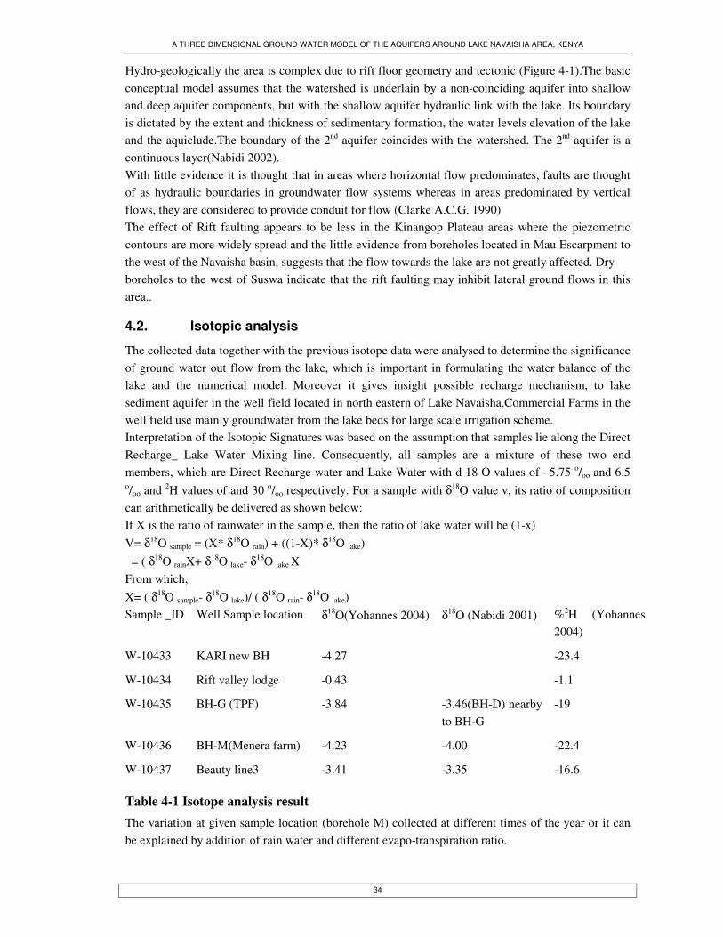
A THREE DIMENSIONAL GROUND WATER MODEL OF THE AQUIFERS AROUND LAKE NAVAISHA AREA, KENYA
34
Hydro-geologically the area is complex due to rift floor geometry and tectonic (Figure 4-1).The basic conceptual model assumes that the watershed is underlain by a non-coinciding aquifer into shallow and deep aquifer components, but with the shallow aquifer hydraulic link with the lake. Its boundary is dictated by the extent and thickness of sedimentary formation, the water levels elevation of the lake and the aquiclude.The boundary of the 2nd aquifer coincides with the watershed. The 2nd aquifer is a continuous layer(Nabidi 2002). With little evidence it is thought that in areas where horizontal flow predominates, faults are thought of as hydraulic boundaries in groundwater flow systems whereas in areas predominated by vertical flows, they are considered to provide conduit for flow (Clarke A.C.G. 1990) The effect of Rift faulting appears to be less in the Kinangop Plateau areas where the piezometric contours are more widely spread and the little evidence from boreholes located in Mau Escarpment to the west of the Navaisha basin, suggests that the flow towards the lake are not greatly affected. Dry boreholes to the west of Suswa indicate that the rift faulting may inhibit lateral ground flows in this area..
4.2. Isotopic analysis
The collected data together with the previous isotope data were analysed to determine the significance of ground water out flow from the lake, which is important in formulating the water balance of the lake and the numerical model. Moreover it gives insight possible recharge mechanism, to lake sediment aquifer in the well field located in north eastern of Lake Navaisha.Commercial Farms in the well field use mainly groundwater from the lake beds for large scale irrigation scheme. Interpretation of the Isotopic Signatures was based on the assumption that samples lie along the Direct Recharge_ Lake Water Mixing line. Consequently, all samples are a mixture of these two end members, which are Direct Recharge water and Lake Water with d 18 O values of –5.75 o/oo and 6.5 o/oo and 2H values of and 30 o/oo respectively. For a sample with δ18O value v, its ratio of composition can arithmetically be delivered as shown below: If X is the ratio of rainwater in the sample, then the ratio of lake water will be (1-x) V= δ18O sample = (X* δ18O rain) + ((1-X)* δ18O lake) = ( δ18O rainX+ δ18O lake- δ18O lake X From which, X= ( δ18O sample- δ18O lake)/ ( δ18O rain- δ18O lake) Sample _ID Well Sample location δ18O(Yohannes 2004) δ18O (Nabidi 2001) %2H (Yohannes
2004)
W-10433 KARI new BH -4.27 -23.4
W-10434 Rift valley lodge -0.43 -1.1
W-10435 BH-G (TPF) -3.84 -3.46(BH-D) nearby to BH-G
-19
W-10436 BH-M(Menera farm) -4.23 -4.00 -22.4
W-10437 Beauty line3 -3.41 -3.35 -16.6
Table 4-1 Isotope analysis result The variation at given sample location (borehole M) collected at different times of the year or it can be explained by addition of rain water and different evapo-transpiration ratio.
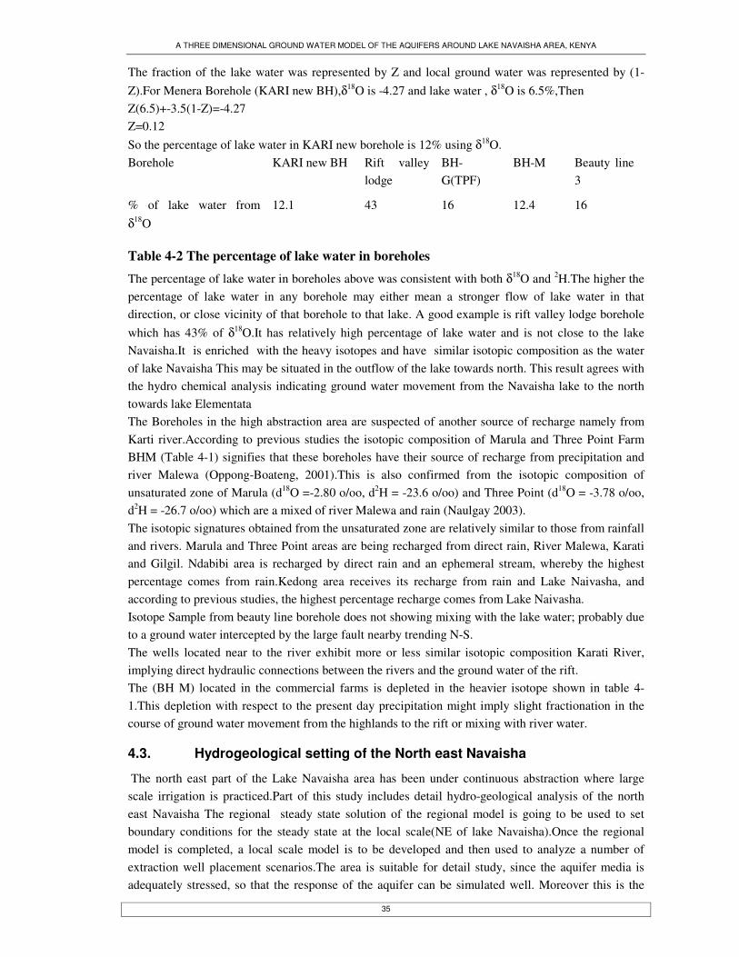
A THREE DIMENSIONAL GROUND WATER MODEL OF THE AQUIFERS AROUND LAKE NAVAISHA AREA, KENYA
35
The fraction of the lake water was represented by Z and local ground water was represented by (1-Z).For Menera Borehole (KARI new BH),δ18O is -4.27 and lake water , δ18O is 6.5%,Then Z(6.5)+-3.5(1-Z)=-4.27 Z=0.12 So the percentage of lake water in KARI new borehole is 12% using δ18O. Borehole KARI new BH Rift valley
lodge BH-G(TPF)
BH-M Beauty line 3
% of lake water from δ18O
12.1 43 16 12.4 16
Table 4-2 The percentage of lake water in boreholes
The percentage of lake water in boreholes above was consistent with both δ18O and 2H.The higher the percentage of lake water in any borehole may either mean a stronger flow of lake water in that direction, or close vicinity of that borehole to that lake. A good example is rift valley lodge borehole which has 43% of δ18O.It has relatively high percentage of lake water and is not close to the lake Navaisha.It is enriched with the heavy isotopes and have similar isotopic composition as the water of lake Navaisha This may be situated in the outflow of the lake towards north. This result agrees with the hydro chemical analysis indicating ground water movement from the Navaisha lake to the north towards lake Elementata The Boreholes in the high abstraction area are suspected of another source of recharge namely from Karti river.According to previous studies the isotopic composition of Marula and Three Point Farm BHM (Table 4-1) signifies that these boreholes have their source of recharge from precipitation and river Malewa (Oppong-Boateng, 2001).This is also confirmed from the isotopic composition of unsaturated zone of Marula (d18O =-2.80 o/oo, d2H = -23.6 o/oo) and Three Point (d18O = -3.78 o/oo, d2H = -26.7 o/oo) which are a mixed of river Malewa and rain (Naulgay 2003). The isotopic signatures obtained from the unsaturated zone are relatively similar to those from rainfall and rivers. Marula and Three Point areas are being recharged from direct rain, River Malewa, Karati and Gilgil. Ndabibi area is recharged by direct rain and an ephemeral stream, whereby the highest percentage comes from rain.Kedong area receives its recharge from rain and Lake Naivasha, and according to previous studies, the highest percentage recharge comes from Lake Naivasha. Isotope Sample from beauty line borehole does not showing mixing with the lake water; probably due to a ground water intercepted by the large fault nearby trending N-S. The wells located near to the river exhibit more or less similar isotopic composition Karati River, implying direct hydraulic connections between the rivers and the ground water of the rift. The (BH M) located in the commercial farms is depleted in the heavier isotope shown in table 4-1.This depletion with respect to the present day precipitation might imply slight fractionation in the course of ground water movement from the highlands to the rift or mixing with river water.
4.3. Hydrogeological setting of the North east Navaisha
The north east part of the Lake Navaisha area has been under continuous abstraction where large scale irrigation is practiced.Part of this study includes detail hydro-geological analysis of the north east Navaisha The regional steady state solution of the regional model is going to be used to set boundary conditions for the steady state at the local scale(NE of lake Navaisha).Once the regional model is completed, a local scale model is to be developed and then used to analyze a number of extraction well placement scenarios.The area is suitable for detail study, since the aquifer media is adequately stressed, so that the response of the aquifer can be simulated well. Moreover this is the

A THREE DIMENSIONAL GROUND WATER MODEL OF THE AQUIFERS AROUND LAKE NAVAISHA AREA, KENYA
36
place where maximum saturated thickness of the lake bed aquifer is found characterized by very high transmissivity.
Figure 4-2 Hypothesis 1.H is the Historic heads and C is the current head While according to the historical piezometric heads of 1980 indicates flow of water towards the lake, situation is different as the current piezometric heads indicate a sink at the location that coincides with the well fields of Manera and Three Point Farm. Three hypotheses have been suggested and discussed by(Nabidi 2002).All hypotheses, except hypothesis 2 assume a two-groundwater aquifers’ system. Apparently hypothesis 2 is invalidated by the existence of a deeper ground water aquifer (see appendix3 showing the borehole log interpretation of the area). Hypothesis 1(Figure 4-2) assumes a by-pass flow pattern with the flow in the two aquifers being in opposite direction. The water in the recharge zone (escarpments) is feed predominantly to the deeper aquifer and flows below the shallow towards the lake. Meanwhile lake water flows towards the escarpment. Based on the isotopic analysis, hypothesis 1 doesn’t hold, because the water extracted from the well field is not predominantly lake water. The δ18O value of borehole M (-3.84) and borehole G (-4.23) doesn’t indicate any significance presence of lake water in the well field whose δ18O value is 6.4%.Besides groundwater from wells on the north side of lake Navisha(C 3366, C3677; Menera farm region) have slightly more radiogenic 87Sr/86Sr ratios (0.70575) than lake Navaisha water (0.70552) where as all the water along the southern shore of the lake have 87Sr/86Sr ratios similar to lake water. Geophysical survey was carried out using Two-dimensional (2D) Resistivity Imaging and Transient Electro-Magnetic (TEM) data on three farms; Three Point, Manera and Home-grown. In all, thirteen Resistivity Imaging Survey profiles of different lengths and 137 Time-Domain EM (TEM) soundings were carried out to model the groundwater system in this area. The formation resistivity physical property, groundwater quality and lithological data were used to model of the aquifer. A representative aquifer model to meet the different needs of the farmers had a formation resistivity range of 12-335 Ohm.m(see figure 4-3). The aquifer exists generally between depths of 20 to 80m in the Three Point Farm. Towards Lake Naivasha in the Manera Farm, the aquifer splits up into two but remains hydraulically connected.The top aquifer occurs between depths of 20-40m and the bottom between 50-80m.The main aquifer materials include fine sands, medium coarse sands, gravels, pebbles and fractured volcanics.Laterally, the high quality and good yield portion of the aquifer occur

A THREE DIMENSIONAL GROUND WATER MODEL OF THE AQUIFERS AROUND LAKE NAVAISHA AREA, KENYA
37
within a radius of approximately 1km from where the Karati river turns from the NW direction to the SW(900 turn).The Karati river has been interpreted to be the main source of recharge into the aquifer.The very low resistivities at depths greater than 80m have been identified as a mixture of clayey materials and saline water.

A THREE DIMENSIONAL GROUND WATER MODEL OF THE AQUIFERS AROUND LAKE NAVAISHA AREA, KENYA
38
Figure 4-3 geological interpretation of the 2-D resistivity imaging model section (Tsiboah 2002)

A THREE DIMENSIONAL GROUND WATER MODEL OF THE AQUIFERS AROUND LAKE NAVAISHA AREA, KENYA
39
According to (Appelo 1996) evapo-transpiration and groundwater flow are two of the many processes affecting water quality including rock weathering. These processes were reflected in the study area with EC and Cl- distributions, as well as the presence of fresh and alkaline water lakes. From data set, EC was generally low in the north and northwest (320 - 700 µS/cm). In the southwest of the lake EC was high (800 - 1560 µS/cm) while in the east EC decreased towards the lake. In the south of the lake EC was between 500 - 1230 µS/cm. There was an increase in EC in the northeast towards the lake (420 - 1560 µS/cm) [See Figure 4-4].
Figure 4-4 Hypothetical cross section profile for NE of the study area (with EC value indicated) The distribution of EC in the area may be related to build up of salts from evapo-transpiration. This is likely to have caused high EC in the Naivasha town area, along the southern border of the lake, as well as in the Crater lake-Oloidien lake areas. Potential evapo-transpiration exceeds rainfall by twofold. Evaporation would result in water being more concentrated with salts and hence, high EC values in shallow groundwater areas. High chloride values around the lake edge, around Crescent island and at Crater lake and Oloidien lake also support the reasoning of evaporation leaving salts behind .Low EC values along the Malewa river, at the head of Karati river, and along the lake edge may have resulted from the mixing of groundwater with river and lake water respectively, pointing to a groundwater-lake water-river water interaction. Based on the flow system the increase in EC towards the lake may be an indication of the up-welling of deep groundwater flow. Low EC generally indicates younger water while high EC suggest old water that has travelled through the aquifer. As indicated from the cross section profile in Figure 4-4, It is possible that old water could be flowing towards the lake and hence the increase of EC towards the lake. Along with increases of EC towards the lake, EC increased from the lake shore toward the southeast from Crescent Island in other data set suggesting that there may be seepage out of the lake. EC may be following the suspected pattern of groundwater flow. Differences in elevation (high areas, lower EC and low areas, higher EC) as well as the presence of warm springs (low EC expected) at the NE end of Figure 4-4 also could justify the distribution of EC in the area, and in particular the NE.Thus, hypothesis 3 is likely to hold, despite the isotopic signature in the well field is not supporting. However this could be explained that the fall of the pieziometric heads in the well field
Lake Centre
Lake
Tuff
NE
High Conductivity Layer
500 1100 990
420
Horizontal Scale 1 cm = 500 m Vertical Scale 1 cm = 250 m
Flow Direction Flow lines Equipotential lines

A THREE DIMENSIONAL GROUND WATER MODEL OF THE AQUIFERS AROUND LAKE NAVAISHA AREA, KENYA
40
below the lake is a recent development.
Figure 4-5 Hypothesis 3 H is the historic head and C is the current head (Nabidi 2002) So it needs time of travel for water from the lake to reach the well field before isotopic signature can
be detected as being over 23 years (estimated using ��
���
�
××=
nedldh
KVe
(Where Ve= Darcian velocity, K is hydraulic conductivity, dh/dl is the hydraulic gradient and ne is the effective porosity) time span that is yet to pass. Moreover, the occurrence of L bend in Karati river course supports the occurrence of a fault system in the well field. Then, besides lake water and direct recharge from the rain, Karati river is possibly a source of recharge to the well field. Hence the isotopic signature could not be dominated by lake water. Thus, hypothesis 3(figure 4-5) is chosen for this study to explain the source of recharge and for the deterioration of the abstraction wells in both quality and quantity.
4.3.1. Well data analysis
Based on the pieziometric maps prior to 1980 of the study area, the groundwater flow direction was towards the Lake navaisha.The figure shows the lake-groundwater-river interaction along the section
that nearly
Section along along Lake-Melewa river
1880
1890
1900
1910
1920
1930
1940
0 1000 2000 3000 4000 5000 6000 7000 8000 9000
Distance from the Lake Navaisha(m)
elev
atio
n(m
) Surface elev
WL_1998
Wl_1968
Milk oulet 4 m lower
Lake
Malewa
4 m lower
includes the well field.
Figure 4-6 Section showing the groundwater level prior and after to high abstraction times
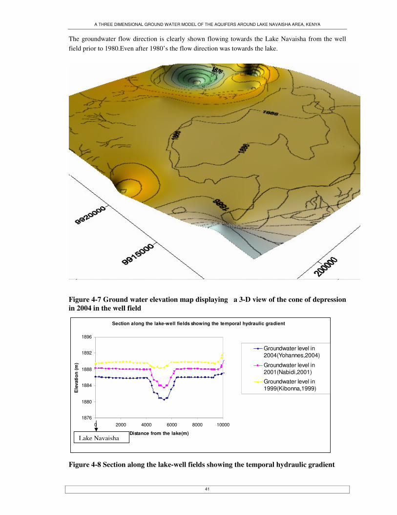
A THREE DIMENSIONAL GROUND WATER MODEL OF THE AQUIFERS AROUND LAKE NAVAISHA AREA, KENYA
41
The groundwater flow direction is clearly shown flowing towards the Lake Navaisha from the well field prior to 1980.Even after 1980’s the flow direction was towards the lake.
Figure 4-7 Ground water elevation map displaying a 3-D view of the cone of depression in 2004 in the well field
Section along the lake-well fields showing the temporal hydraulic gradient
1876
1880
1884
1888
1892
1896
0 2000 4000 6000 8000 10000
Distance from the lake(m)
Ele
vatio
n (m
)
Groundwater level in2004(Yohannes,2004)
Groundwater level in2001(Nabidi,2001)
Groundwater level in1999(Kibonna,1999)
Figure 4-8 Section along the lake-well fields showing the temporal hydraulic gradient
Lake Navaisha

A THREE DIMENSIONAL GROUND WATER MODEL OF THE AQUIFERS AROUND LAKE NAVAISHA AREA, KENYA
42
The section for figure 4-10 was taken from the lake towards north east where cone of depression is shown in figure 4-9.Cone of depression is well developed in the commercial farms, typically in the Panda flower farm. The flow direction was reversed due to continuous abstraction in the well fields in the recent years dated back since the last 6 years .It is uncertain that whether the reduction in static water level is a response to changing lake water levels or is due to abstraction. However given that in general the drop in ground water levels is greater than in the lake, it is likely that either abstraction has exceeded through flow or recharge parameters have changed. Lake level fallen to 1886.7, a drop of 3.3 m over the past 20 years. While the panda flower boreholes had fallen from 3 m to 8 m over 6 years shown in figure 4-9 with significant cone of depression for the year 2004. Referring to table 6-8, 16.7 MCM/yr is 31% of estimated water budget seepage inflow in an average year. This a significant proportion of the total ,and one would expect to observe changes in ground water conditions as a consequence of such abstraction. These changes would include the declining water levels and progressive salinazation of ground water that have been observed at Menera.In addition to falling water levels and rising salinity, impacts may include temporary or permanent compaction of the aquifer matrix (indication by a reduction in transmissivity).This would lead to a greater drawdown for a given discharge and would accelerate the rate of water quality deterioration if this was due to upward or lateral migration Conditions Wet year Average year Dry year Goldson(1993)
Inflows(MCM/yr)
Direct rainfall 140.8 72.9 45 72.96
Melewa inflows 378 153 53
Gilgil inflows 74 24 3.2
Karati inflows 6.5 2.1 .28
Other surface inflow 117.8 77.9 34.2
Inflow seepage 54 54 32
150
Total inflows 771.1 383.9 167.7 49
271.96
Outflows(MCM/yr)
Evapotranspirative loss 38.5 26.7 21.9 10.8
Direct evaporation losses
229 183.5 177.8 162.0
Outflow seepage 54 54 32 55
Abstraction(estimated) 33.8 44.6 53.2 47.9
Total outflows 335.3 308.8 284.9 275.7
Balance +415.8 +75 -117.2 -3.74
Table 4-3 Navaisha basin water budget(After : LNROA 1996:(GoldsonJohn 1993)

A THREE DIMENSIONAL GROUND WATER MODEL OF THE AQUIFERS AROUND LAKE NAVAISHA AREA, KENYA
43
Water chemistry change may be a response to excessive abstraction and may be aggravated by drought. It has long been known that the abstraction of large amount of ground water can lead to deterioration of ground water quality. However it is usually because the hydraulic head distribution created by one or more pumping boreholes encourages bodies of low quality water to move in to the aquifer .The low quality water can have many different origins.
• Upcoming of deep connate water. • Downward leakage of poor quality surface waters. • Percolation of irrigation waters • Saline intrusion
From the geophysical survey the very low resistivities at depths greater than 80 metres have been identified as a mixture of clayey materials and saline water (see figure 4-3).This warns the danger of up conning of deep saline water that exists particularly in areas away from Karati river and in areas near Lake Navaisha.Ground water quality also deteriorates with larger distance away from the river to the north and northwest. However (Nabidi 2002)concluded the deterioration of water quality with time is a consequence of radial interception of cone of depression with salt lenses caused by high rate pumping rather than human induced upconing.He plotted EC of wells against the sampling time to study the temporal variation of the water chemistry and their EC values against yield and depth to understand the correlation between EC and each of them. The plot of yield and depth against EC indicates that there is neither correlation between yield and EC nor between depth and EC. Apparently, evidence of hydraulic interconnection between the aquifer and the lake is shown in the similarity between the lake and well hydrographs. And by comparison of slopes or hydraulic gradients of lines of wells perpendicular and parallel to the lake’s, the slope of the line of wells perpendicular to the lake is much steeper than the slopes of the lines of wells parallel to the lake, indicating that the cone of depression was distorted by the presence of the lake, and that the water from the lake was diverted in to the cone of depression by induced infiltration Also assuming that the lake bed aquifer is similar in genesis to other unconsolidated sedimentary aquifers, it is possible to assume that changes are taking place as a consequence of heavy abstraction. Overall, the source of the poor water quality could be any of the above mentioned sources or a combination of these. Given the cyclic history of the Navaisha basin, it is possible that evaporate dposits were laid down during interpluvial stages in the basin history.
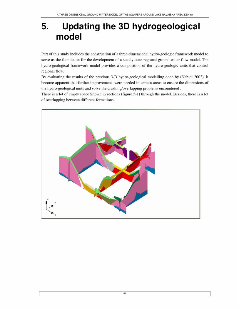
A THREE DIMENSIONAL GROUND WATER MODEL OF THE AQUIFERS AROUND LAKE NAVAISHA AREA, KENYA
44
5. Updating the 3D hydrogeological model
Part of this study includes the construction of a three-dimensional hydro-geologic framework model to serve as the foundation for the development of a steady-state regional ground-water flow model. The hydro-geological framework model provides a composition of the hydro-geologic units that control regional flow. By evaluating the results of the previous 3-D hydro-geological modelling done by (Nabidi 2002), it become apparent that further improvement were needed in certain areas to ensure the dimensions of the hydro-geological units and solve the crushing/overlapping problems encountered . There is a lot of empty space Shown in sections (figure 5-1) through the model. Besides, there is a lot of overlapping between different formations.

A THREE DIMENSIONAL GROUND WATER MODEL OF THE AQUIFERS AROUND LAKE NAVAISHA AREA, KENYA
45
Figure 5-1 Section through the solid model The 3-D representation of geology was tried using the Additive and subtractive approach executed with “set operations” in GMS software. But it could not be done at any level as the computer was continually “crushing” (Nabidi 2002).Thus; the new method of subsurface characterization that honours the stratigraphy introduced in the latest GMS 5.0 was used to solve empty spaces and overlapping problems(Figure 5-2) Steps involved building solid model 1. Integration of 2D data 2. Supplement of cross-sections together with set of borehole data (log) 4. Construction of horizon by assigning horizon ID to the contact of Boreholes and 5. Representation of solids. TIN (Triangular irregular Network) was used for surface modelling and representing geological unit besides to constructing solid model. Meanwhile user defined borehole cross section was used to further control the, horizon to solid model process and modelling pinch outs using the represent missing horizon implicitly.
Figure 5-2 cross section from the solid model built using horizon method shown without empty space and overlapping problems
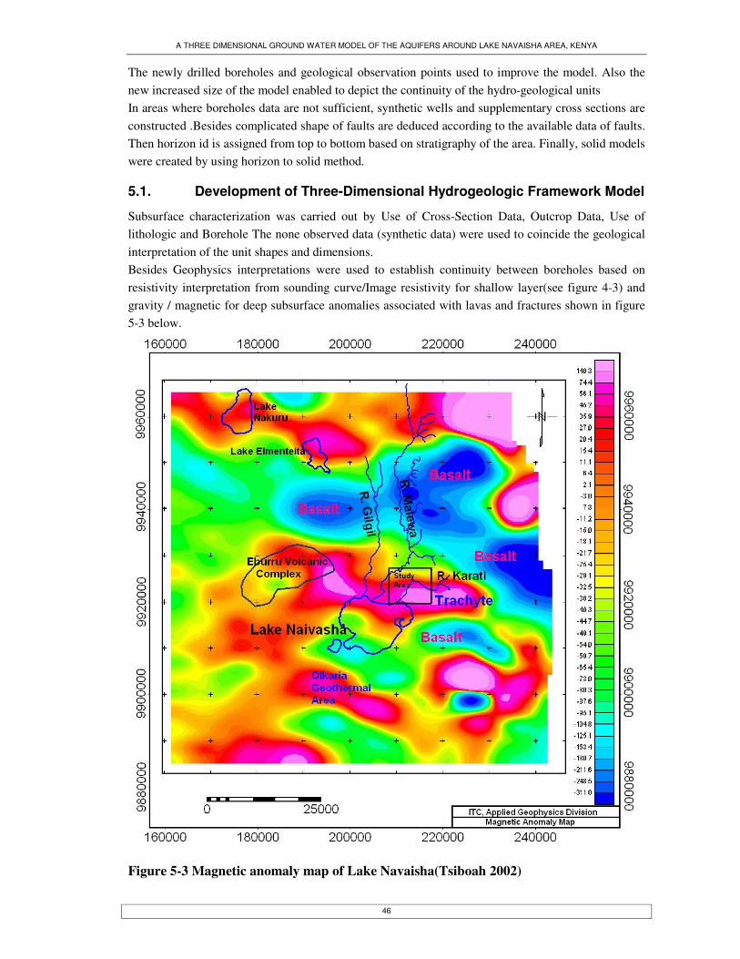
A THREE DIMENSIONAL GROUND WATER MODEL OF THE AQUIFERS AROUND LAKE NAVAISHA AREA, KENYA
46
The newly drilled boreholes and geological observation points used to improve the model. Also the new increased size of the model enabled to depict the continuity of the hydro-geological units In areas where boreholes data are not sufficient, synthetic wells and supplementary cross sections are constructed .Besides complicated shape of faults are deduced according to the available data of faults. Then horizon id is assigned from top to bottom based on stratigraphy of the area. Finally, solid models were created by using horizon to solid method.
5.1. Development of Three-Dimensional Hydrogeologic Framework Model
Subsurface characterization was carried out by Use of Cross-Section Data, Outcrop Data, Use of lithologic and Borehole The none observed data (synthetic data) were used to coincide the geological interpretation of the unit shapes and dimensions. Besides Geophysics interpretations were used to establish continuity between boreholes based on resistivity interpretation from sounding curve/Image resistivity for shallow layer(see figure 4-3) and gravity / magnetic for deep subsurface anomalies associated with lavas and fractures shown in figure 5-3 below.
Figure 5-3 Magnetic anomaly map of Lake Navaisha(Tsiboah 2002)
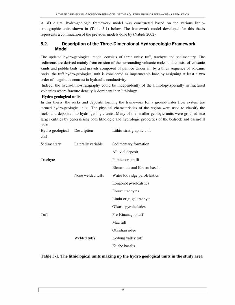
A THREE DIMENSIONAL GROUND WATER MODEL OF THE AQUIFERS AROUND LAKE NAVAISHA AREA, KENYA
47
A 3D digital hydro-geologic framework model was constructed based on the various lithio-stratigraphic units shown in (Table 5-1) below. The framework model developed for this thesis represents a continuation of the previous models done by (Nabidi 2002).
5.2. Description of the Three-Dimensional Hydrogeologic Framework Model
The updated hydro-geological model consists of three units: tuff, trachyte and sedimentary. The sediments are derived mainly from erosion of the surrounding volcanic rocks, and consist of volcanic sands and pebble beds, and gravels composed of pumice Underlain by a thick sequence of volcanic rocks, the tuff hydro-geological unit is considered as impermeable base by assigning at least a two order of magnitude contrast in hydraulic conductivity Indeed, the hydro-litho-stratigraphy could be independently of the lithiology.specially in fractured volcanics where fracture density is dominant than lithiology. Hydro-geological units In this thesis, the rocks and deposits forming the framework for a ground-water flow system are termed hydro-geologic units.. The physical characteristics of the region were used to classify the rocks and deposits into hydro-geologic units. Many of the smaller geologic units were grouped into larger entities by generalizing both lithologic and hydrologic properties of the bedrock and basin-fill units. Hydro-geological unit
Description Lithio-stratigraphic unit
Laterally variable Sedimentary formation Sedimentary
Alluvial deposit
Pumice or lapilli
Elementata and Eburru basalts
None welded tuffs Water loo ridge pyrolclastics
Longonot pyrolcalstics
Eburru trachytes
Limlu or gilgel trachyte
Trachyte
Olkaria pyrolcalstics
Pre-Kinanagop tuff
Mau tuff
Obsidian ridge
Welded tuffs Kedong valley tuff
Tuff
Kijabe basalts
Table 5-1. The lithiological units making up the hydro geological units in the study area
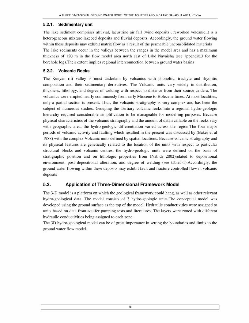
A THREE DIMENSIONAL GROUND WATER MODEL OF THE AQUIFERS AROUND LAKE NAVAISHA AREA, KENYA
48
5.2.1. Sedimentary unit
The lake sediment comprises alluvial, lacustrine air fall (wind deposits), reworked volcanic.It is a heterogeneous mixture lakebed deposits and fluvial deposits. Accordingly, the ground water flowing within these deposits may exhibit matrix flow as a result of the permeable unconsolidated materials The lake sediments occur in the valleys between the ranges in the model area and has a maximum thickness of 120 m in the flow model area north east of Lake Navaisha (see appendix.3 for the borehole log).Their extent implies regional interconnection between ground water basins
5.2.2. Volcanic Rocks
The Kenyan rift valley is most underlain by volcanics with phonoltic, trachyte and rhyolitic composition and their sedimentary derivatives. The Volcanic units vary widely in distribution, thickness, lithology, and degree of welding with respect to distance from their source caldera. The volcanics were erupted nearly continuously from early Miocene to Holecene times. At most localities, only a partial section is present. Thus, the volcanic stratigraphy is very complex and has been the subject of numerous studies. Grouping the Tertiary volcanic rocks into a regional hydro-geologic hierarchy required considerable simplification to be manageable for modelling purposes. Because physical characteristics of the volcanic stratigraphy and the amount of data available on the rocks vary with geographic area, the hydro-geologic differentiation varied across the region.The four major periods of volcanic activity and faulting which resulted in the present was discussed by (Baker et al 1988) with the complex Volcanic units defined by spatial locations. Because volcanic stratigraphy and its physical features are genetically related to the location of the units with respect to particular structural blocks and volcanic centres, the hydro-geologic units were defined on the basis of stratigraphic position and on lithologic properties from (Nabidi 2002)related to depositional environment, post depositional alteration, and degree of welding (see table5-1).Accordingly, the ground water flowing within these deposits may exhibit fault and fracture controlled flow in volcanic deposits
5.3. Application of Three-Dimensional Framework Model
The 3-D model is a platform on which the geological framework could hang, as well as other relevant hydro-geological data. The model consists of 3 hydro-geologic units.The conceptual model was developed using the ground surface as the top of the model. Hydraulic conductivities were assigned to units based on data from aquifer pumping tests and literatures. The layers were zoned with different hydraulic conductivities being assigned to each zone. The 3D hydro-geological model can be of great importance in setting the boundaries and limits to the ground water flow model.

A THREE DIMENSIONAL GROUND WATER MODEL OF THE AQUIFERS AROUND LAKE NAVAISHA AREA, KENYA
49
Figure 5-4 Ortho view of the updated solid model
Figure 5-5 North-south cross section through the central part of the model area (Note that the continuity of the lake sediment the beyond the Navaisha watershed is shown)
5.4. Evaluating the Model
The 3D framework was evaluated once it was constructed. These evaluations consisted of visual inspection of the gridded surfaces and various mathematical manipulations (neighbourhood, inverse weight) of the grids to assess extent and thickness of the hydro-geologic units. The model was sliced vertically along the grid cells corresponding to a series of north-south and east-west cross sections,
Lake Elementaita Lake Navaisha
Lake Navaisha
Lake Elementata

A THREE DIMENSIONAL GROUND WATER MODEL OF THE AQUIFERS AROUND LAKE NAVAISHA AREA, KENYA
50
creating a fence diagram. The model sections retain the basic lithology and geometrical characteristics needed for the numerical ground-water flow modelling. Discrepancies can be seen on some of the model surface. The gridding algorithm tends to extrapolate grids one grid cell beyond the limits of the data. The flow modelling process also provided a mechanism to evaluate the hydro geological frame work. Here is a listing of the modifications made during the flow model calibration process: 1.The surface elevation of the boreholes used before by(Nabidi 2002) did not match with the surface topography generated from the new DEM(Derived from SRTM radar).Thus, the elevation of the boreholes were adjusted accordingly. 2. Sedimentary unit grids in the area of Elementata basin were over extrapolated from the borehole data used to produce the gridded interpretation. The Sedimentary grid in these areas was modified to conform more to the extent of the sedimentary depicted on the mapped outcrop data and geological observation points. Over representation of sedimentation is observed in the hydro-geological frame work .Indeed, these extensions are thin and above the water table, they are thought to have very little effect on ground-water flow modelling.
5.5. Attribution of Model Cells
The GMS software allows each cell to have multiple attributes.The software automatically assigned basic attributes to each cell to define its row, column, sequence, layer, depth, and altitude. The cells were further attributed to define their hydro-geologic units and the top and bottom of the hydro-geologic unit. In the new layer property package (LPF), layer hydraulic property entry can be assigned using data array and material id method.The data array method was selected since it allows representing faults using coverage’s in the map module.However the Block centred flow package (BCF) has only one option using material id which is hardly possible to represent the networked faults of the rift system area well and for further optimization of the parameters using inverse modelling.

A THREE DIMENSIONAL GROUND WATER MODEL OF THE AQUIFERS AROUND LAKE NAVAISHA AREA, KENYA
51
6. Conceptual model
Development of a conceptual model is one of the initial steps. The purpose of developing conceptual model are to develop a better understanding of site conditions, to define the ground water problem for development of a numerical model and to aid in selecting a suitable numerical model(Spitez 1996).The conceptual model includes the potentiometric surface, hydraulic properties, and recharge and discharge components. Developing of conceptual model is the most important part of the modelling process. Its significance is to simplify the field situation and to organize associated field data for easy analysis of the system.
Figure 6-1 Satellite image draped over the Triangulation Irregular Network (TIN) showing the 3-D view of the study area including subsurface characterization using boreholes to build solid model, done in GMS software. It is critical that the conceptual model be a valid representation of the important hydro-geologic condition and involves definition of the hydro-stratigraphic units(The hydro-geological units are described in the previous chapter 5), water balances and flow system.This involves identifying sources of recharge, discharge and variation of aquifer properties, variation of hydraulic heads and the relationship between surface water and ground water. The conceptual model and simplifying assumptions are discussed in this section.

A THREE DIMENSIONAL GROUND WATER MODEL OF THE AQUIFERS AROUND LAKE NAVAISHA AREA, KENYA
52
Figure 6-2. A 2D schematic cross section of the conceptual model drawn from the Mau Scarps(western) to the South Kinangop Fault (eastern) through the Lake Naivasha basin. Not drawn to scale
The flow system of the area is defined by regional, intermediate and local flow system.The deep and intermediate ground water flow may be controlled by extensive and pervasive faults and fractures. The available hydro-metrological, hydro-geological and land use data has been used to identify the component of ground water balance in the lake Elementata-nakuru and Navaisha area. As an initial estimate of the model, the water balance components identified have been included in the model. This means recharge from precipitation will be applied, flows across boundaries will be considered, the interaction with lake will be modeled.water balance quantities assigned in to the model or computed will have to be closely checked with realistic ranges.
6.1. Potentiometric surface
Average potentiometric surfaces were estimated for the analysis period (1932-98) (Appendix 6 and 7) for calibration of the steady-state model. The flow patterns are basically similar with the regional ground water contour map of figure 2-3. The ground water contour map was adjusted on the basis of hydro chemical and isotope data as part of effort in developing conceptual ground water model. Water levels during 1998 and 2001 were documented by (Ower 2000) and (Nabidi 2002)respectively.
6.2. Representation of hydraulic properties
Hydraulic properties of the Shallow and deep aquifers in and near the study area have been estimated by previous investigators. For the aquifer located nearby to the lake, hydraulic conductivities in south-central South, estimated from 205 well logs, ranged from 3.6 to 160 metres per day, with an average of 30 metres per day (Clarke A.C.G. 1990). For the lake sediment aquifer, hydraulic conductivities determined from aquifer tests in Menera and panda flower farms from 7.9 to 21.6 metres per day(Mcann 1974)
Kz=very low
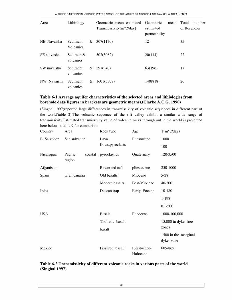
A THREE DIMENSIONAL GROUND WATER MODEL OF THE AQUIFERS AROUND LAKE NAVAISHA AREA, KENYA
53
Area Lithiology Geometric mean estimated Transmissivity(m^2/day)
Geometric mean estimated permeability
Total number of Boreholes
NE Navaisha Sediment & Volcanics
307(1170) 12 35
SE naivasha Sediment& volcanics
502(3082) 20(114) 22
SW navaisha Sediment & volcanics
297(940) 63(196) 17
NW Navaisha Sediment & volcanics
1601(5308) 148(818) 26
Table 6-1 Average aquifer characteristics of the selected areas and lithiologies from borehole data(figures in brackets are geometric means),(Clarke A.C.G. 1990) (Singhal 1997)reported large differences in transmissivity of volcanic sequences in different part of the world(table 2).The volcanic sequence of the rift valley exhibit a similar wide range of transmissivity.Estimated transmissivity value of volcanic rocks through out in the world is presented here below in table.9.for comparison Country Area Rock type Age T(m^2/day)
El Salvador San salvador Lava flows,pyroclasts
Pliestocene 1000
100
Nicarogua Pacific coastal region
pyroclastics Quaternary 120-3500
Afganistan Reworked tuff pliestocene 250-1000
Spain Gran canaria Old basalts
Modern basalts
Miocene
Post-Miocene
5-28
40-200
India Deccan trap Early Eocene 10-180
1-198
0.1-500
USA Basalt
Tholietic basalt
basalt
Plieocene 1000-100,000
15,000 in dyke free zones
1500 in the marginal dyke zone
Mexico Fissured basalt Pleistocene-Holocene
605-865
Table 6-2 Transmissivity of different volcanic rocks in various parts of the world (Singhal 1997)
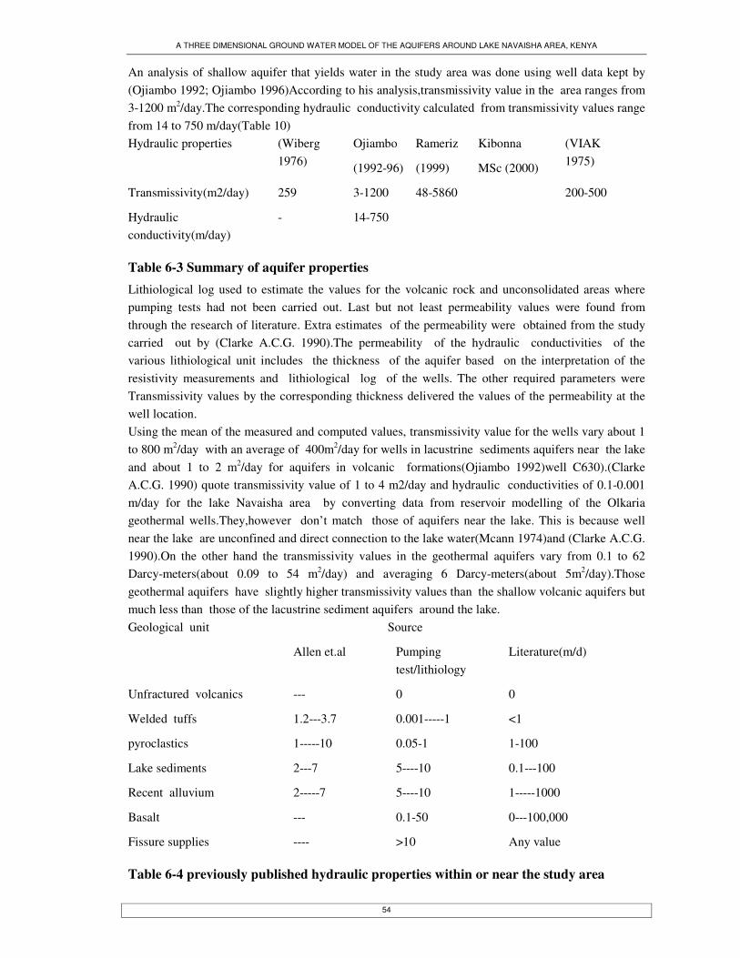
A THREE DIMENSIONAL GROUND WATER MODEL OF THE AQUIFERS AROUND LAKE NAVAISHA AREA, KENYA
54
An analysis of shallow aquifer that yields water in the study area was done using well data kept by (Ojiambo 1992; Ojiambo 1996)According to his analysis,transmissivity value in the area ranges from 3-1200 m2/day.The corresponding hydraulic conductivity calculated from transmissivity values range from 14 to 750 m/day(Table 10) Hydraulic properties (Wiberg
1976) Ojiambo
(1992-96)
Rameriz
(1999)
Kibonna
MSc (2000)
(VIAK 1975)
Transmissivity(m2/day) 259 3-1200 48-5860 200-500
Hydraulic conductivity(m/day)
- 14-750
Table 6-3 Summary of aquifer properties Lithiological log used to estimate the values for the volcanic rock and unconsolidated areas where pumping tests had not been carried out. Last but not least permeability values were found from through the research of literature. Extra estimates of the permeability were obtained from the study carried out by (Clarke A.C.G. 1990).The permeability of the hydraulic conductivities of the various lithiological unit includes the thickness of the aquifer based on the interpretation of the resistivity measurements and lithiological log of the wells. The other required parameters were Transmissivity values by the corresponding thickness delivered the values of the permeability at the well location. Using the mean of the measured and computed values, transmissivity value for the wells vary about 1 to 800 m2/day with an average of 400m2/day for wells in lacustrine sediments aquifers near the lake and about 1 to 2 m2/day for aquifers in volcanic formations(Ojiambo 1992)well C630).(Clarke A.C.G. 1990) quote transmissivity value of 1 to 4 m2/day and hydraulic conductivities of 0.1-0.001 m/day for the lake Navaisha area by converting data from reservoir modelling of the Olkaria geothermal wells.They,however don’t match those of aquifers near the lake. This is because well near the lake are unconfined and direct connection to the lake water(Mcann 1974)and (Clarke A.C.G. 1990).On the other hand the transmissivity values in the geothermal aquifers vary from 0.1 to 62 Darcy-meters(about 0.09 to 54 m2/day) and averaging 6 Darcy-meters(about 5m2/day).Those geothermal aquifers have slightly higher transmissivity values than the shallow volcanic aquifers but much less than those of the lacustrine sediment aquifers around the lake. Geological unit Source
Allen et.al Pumping test/lithiology
Literature(m/d)
Unfractured volcanics --- 0 0
Welded tuffs 1.2---3.7 0.001-----1 <1
pyroclastics 1-----10 0.05-1 1-100
Lake sediments 2---7 5----10 0.1---100
Recent alluvium 2-----7 5----10 1-----1000
Basalt --- 0.1-50 0---100,000
Fissure supplies ---- >10 Any value
Table 6-4 previously published hydraulic properties within or near the study area
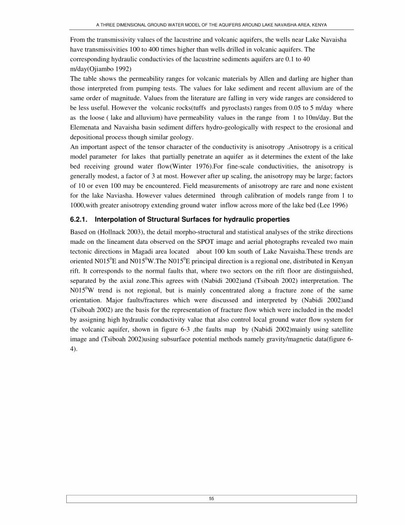
A THREE DIMENSIONAL GROUND WATER MODEL OF THE AQUIFERS AROUND LAKE NAVAISHA AREA, KENYA
55
From the transmissivity values of the lacustrine and volcanic aquifers, the wells near Lake Navaisha have transmissivities 100 to 400 times higher than wells drilled in volcanic aquifers. The corresponding hydraulic conductivies of the lacustrine sediments aquifers are 0.1 to 40 m/day(Ojiambo 1992) The table shows the permeability ranges for volcanic materials by Allen and darling are higher than those interpreted from pumping tests. The values for lake sediment and recent alluvium are of the same order of magnitude. Values from the literature are falling in very wide ranges are considered to be less useful. However the volcanic rocks(tuffs and pyroclasts) ranges from 0.05 to 5 m/day where as the loose ( lake and alluvium) have permeability values in the range from 1 to 10m/day. But the Elemenata and Navaisha basin sediment differs hydro-geologically with respect to the erosional and depositional process though similar geology. An important aspect of the tensor character of the conductivity is anisotropy .Anisotropy is a critical model parameter for lakes that partially penetrate an aquifer as it determines the extent of the lake bed receiving ground water flow(Winter 1976).For fine-scale conductivities, the anisotropy is generally modest, a factor of 3 at most. However after up scaling, the anisotropy may be large; factors of 10 or even 100 may be encountered. Field measurements of anisotropy are rare and none existent for the lake Naviasha. However values determined through calibration of models range from 1 to 1000,with greater anisotropy extending ground water inflow across more of the lake bed (Lee 1996)
6.2.1. Interpolation of Structural Surfaces for hydraulic properties
Based on (Hollnack 2003), the detail morpho-structural and statistical analyses of the strike directions made on the lineament data observed on the SPOT image and aerial photographs revealed two main tectonic directions in Magadi area located about 100 km south of Lake Navaisha.These trends are oriented N0150E and N0150W.The N0150E principal direction is a regional one, distributed in Kenyan rift. It corresponds to the normal faults that, where two sectors on the rift floor are distinguished, separated by the axial zone.This agrees with (Nabidi 2002)and (Tsiboah 2002) interpretation. The N0150W trend is not regional, but is mainly concentrated along a fracture zone of the same orientation. Major faults/fractures which were discussed and interpreted by (Nabidi 2002)and (Tsiboah 2002) are the basis for the representation of fracture flow which were included in the model by assigning high hydraulic conductivity value that also control local ground water flow system for the volcanic aquifer, shown in figure 6-3 ,the faults map by (Nabidi 2002)mainly using satellite image and (Tsiboah 2002)using subsurface potential methods namely gravity/magnetic data(figure 6-4).
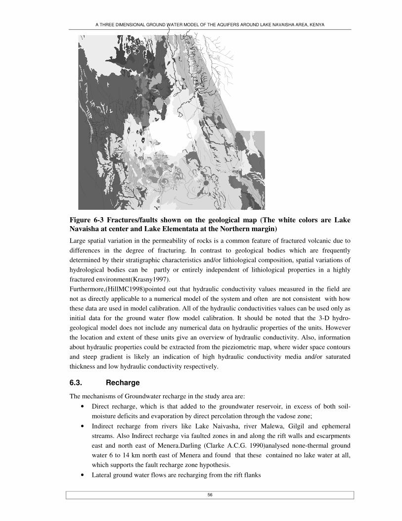
A THREE DIMENSIONAL GROUND WATER MODEL OF THE AQUIFERS AROUND LAKE NAVAISHA AREA, KENYA
56
Figure 6-3 Fractures/faults shown on the geological map (The white colors are Lake Navaisha at center and Lake Elementata at the Northern margin) Large spatial variation in the permeability of rocks is a common feature of fractured volcanic due to differences in the degree of fracturing. In contrast to geological bodies which are frequently determined by their stratigraphic characteristics and/or lithiological composition, spatial variations of hydrological bodies can be partly or entirely independent of lithiological properties in a highly fractured environment(Krasny1997). Furthermore,(HillMC1998)pointed out that hydraulic conductivity values measured in the field are not as directly applicable to a numerical model of the system and often are not consistent with how these data are used in model calibration. All of the hydraulic conductivities values can be used only as initial data for the ground water flow model calibration. It should be noted that the 3-D hydro-geological model does not include any numerical data on hydraulic properties of the units. However the location and extent of these units give an overview of hydraulic conductivity. Also, information about hydraulic properties could be extracted from the pieziometric map, where wider space contours and steep gradient is likely an indication of high hydraulic conductivity media and/or saturated thickness and low hydraulic conductivity respectively.
6.3. Recharge
The mechanisms of Groundwater recharge in the study area are: • Direct recharge, which is that added to the groundwater reservoir, in excess of both soil-
moisture deficits and evaporation by direct percolation through the vadose zone; • Indirect recharge from rivers like Lake Naivasha, river Malewa, Gilgil and ephemeral
streams. Also Indirect recharge via faulted zones in and along the rift walls and escarpments east and north east of Menera.Darling (Clarke A.C.G. 1990)analysed none-thermal ground water 6 to 14 km north east of Menera and found that these contained no lake water at all, which supports the fault recharge zone hypothesis.
• Lateral ground water flows are recharging from the rift flanks

A THREE DIMENSIONAL GROUND WATER MODEL OF THE AQUIFERS AROUND LAKE NAVAISHA AREA, KENYA
57
• Recharge from depressions, like Lake Naivasha on the rift floor • Localized recharge from horizontal surface concentration of water in the absence of well
defined channels as shown in the young Eburru volcanics and particularly on the volcanic centres them selves.
To make a reliable assessment of the groundwater recharge normally requires an adequate amount of good quality data on geology, geomorphology, hydrology, vegetation, topography and climate, (Meijerink 1994). The availability of recharge estimate techniques differs climatically.Sources and processes of recharge in humid areas are different compared with (semi-)arid areas; hence the need to precede from a well-defined conceptualisation of different recharge processes is essential, as is the need to use more than one technique for verification of results. Generally the most factors contributing to recharge in the area are rainfall, evapo-transpiration rates and soil types. The area experiences an annual rainfall of 640mm, which is characteristic of a semi arid climate. Since the potential evapo-transpiration of the area was estimated to be higher than rainfall, direct recharge is not a permanent process in the area, but a process which occurs during rain seasons and, only when there is high intensity.. The Pleistocene pyroclastics that flank the Mau and Abdare escarpments appear relatively absorptive and doubtless transmit infiltrating precipitation and run off to the underlying fracture and fissure systems of less absorptive and permeable rocks. Such recharge probably also occurs where quaternary pyroclastics occur such as in the Eburru area(Mcann 1974). The natural areas around Kedong received the highest recharge (43.75mmyr-1), followed by Marula (33.75mmyr-1).Ndabibi and Three Point receives the lowest, 0.69mmyr-1and 4.38mmyr-1 respectively. The highest recharge was received in the year 1998, during El Nino period. The big variation in recharge is associated with the different types of vegetations and soils in the study area. Local name Location Recharge(mm/day)
UTM_X UTM_Y Min Max
Average recharge(mm/yr)
Kedong 209691 9908544 0 1.9 14.29
Ndabaib 194490 9914863 0 .18 0.03
TPF 213403 9924948 0 .024 2.57
Marula 208444 9930840 0 0.28 7.43
Table 6-5 Direct recharge estimate from SWAP model (1990-1997), before El Nino, by (Nalugya 2003) Local name Location Recharge(mm/day)
UTM_X UTM_Y Min Max
Average recharge(mm/yr)
Kedong 209691 9908544 0 7 43.75
Ndabibi 194490 9914863 0 .27 0.69
TPF 213403 9924948 0 0.1 4.38
Marula 208444 9930840 0 5.5 33.75
Table 6-6 Direct recharge estimate from SWAP model (1997-1998), after El Niño, by (Nalugya 2003)

A THREE DIMENSIONAL GROUND WATER MODEL OF THE AQUIFERS AROUND LAKE NAVAISHA AREA, KENYA
58
The groundwater recharge in the study area is influenced by climate, soils, vegetation, lithology and geomorphology of the area..The area experiences an annual rainfall of 640mm. Since the potential evapo-transpiration (1700mm) of the area is much higher than rainfall, direct recharge is not a permanent process in the area, but a process which occurs during rain seasons and, only when there are high intensities, this explains those periods during model simulations which show zero bottom flux. From the previous studies, the aquifers of Marula and Three Point, in the northern part of the study area obtain their recharge from Precipitation and river Malewa; the largest percentage comes from the river.Ndabibi plains, is recharged by precipitation and Kedong area, by Lake Naivasha and precipitation, the highest percentage being contributed by the Lake. The main factors influencing the water movement in the unsaturated zone are the rooting density and depth of vegetation, and the types of soil layers in the profiles. Most part of the study area is flat, with no indication of valleys, hence no runoff. So when it rains, due to high rate of evaporation, much of it evaporates and that which remains infiltrates, through the pumice sand to the deeper parts of unsaturated zone.If a water flux is obtained at a depth in a profile where no further abstraction by roots occur, it is estimated to be equal to groundwater recharge (Allison 1987). In Ndabibi, Marula and three point areas, the water flux below the rooting depth of grass is still affected by the presence of acacia trees, whose roots continue extracting water from deeper parts of the unsaturated zone and could even go up to the water table. The total amount consumed by these trees depends on their percentage coverage in the respective areas. A simple 1-D mixing model simulated direct recharge in the southern part of the lake Naivasha aquifer, 10 km away from the lake. From the piezometric map, the isotopic signatures of boreholes located within this area; with heads between 1888-1884 metres were used in model calibration (Naulgay 2003). These were taken as measured values during the simulation. Their signatures range between 6 - 3 o/oo for 18O and 36–18 o/oo for 2H. From the simple 1-D mixed model, the simulated recharge between these limits was of the range (3.65–25.55) mmyear-1, giving an average recharge of14.60 mmyear1, which figure correlates well with the direct recharge simulated from SWAP model before El Nino (Table 6.1), in Kedong area.This is assumed to be the average contribution of direct recharge towards southern part of the lake aquifer, in a radius of 10km.The lake water percentages agree with the previous estimates on lake water contribution (Oppong-Boateng 2001)towards the aquifer. The evaluation of validity of the simple model with measured isotopic values was based on a general piezometric range (1888-1884), due to lack of independent piezometric heads for each borehole. Recharge in (semi-) areas can be determined through the vadose zone from direct calculation of water fluxes, either by applying or establishing a vadose-zone water balance on the basis of soil, climate, and vegetation data. However this is not a straightforward process, since the small recharge calculated from the difference between rainfall and actual evapo-transpiration is still less than the accuracy rangeof recharge (Simmers 2002). The ephemeral streams in the study areas can also be source of recharge especially during dry seasons when ephemeral rivers terminate in depressions groundwater recharge can also occur. In this case topography of the region plays a dominant role. The low values of direct recharge are caused by mainly two factors, the little and irregular distribution of rain and, high rates of evapo-transpiration in the study area. And not every rainfall event causes recharge, direct recharge only occurs during wet seasons and only when there is a heavy storm. The natural areas around Kedong received the highest recharge (43.75mm/yr), followed by Marula (33.75 mm/yr). Ndabibi and Three Point farm receives the lowest, 0.69 mmyr-1and 4.38mmyr-1 respectively.

A THREE DIMENSIONAL GROUND WATER MODEL OF THE AQUIFERS AROUND LAKE NAVAISHA AREA, KENYA
59
The highest recharge was received in the year 1998, during El Nino period. The big variation in recharge is associated with the different types of vegetations and soils in the study area. Groundwater recharge may be also estimated on the basis of seasonal changes in ground water levels, but since the areal extent of recharge areas is essentially unknown such estimate must be considered only as indication of magnitude of recharge. Apparent recharge may be estimated on the basis of the relation ship
�= SyhAR **
Where R=ground water recharge A=area
�h =sum of seasonal increase in ground water level
Sy =Specific yield of water yielding materials Assuming rather conservative specific yield values of 5% for lake sediments and quaternary alluvium,3% for recent and Pleistocene pyroclastics and 1% for the volcanic rocks, the apparent annual recharge is estimated to be: Catchment Apparent recharge(*10^6 m3)
Naivasha 151
Nakuru-Elementata 116
Table 6-7 Apparent recharge estimated by (Mcann 1974) (Graham 1998)compared the average ground water inflow from the northern and eastern catchment’s of the Navaisha basin using changes in EC along the longitudinal profile with a decrease in ground water inflow of 1.3 mm/year along these Malawa river tributaries. This could be attributed to grid faulting along the rift floor which acts as conduits and channel flow along the rift floor. However there is an indication of ground water inflow along the main tributaries of the Malewa and there is an increase in inflow of 1.9 mm/year. This additional inflow is presumed to come from the area of the Kinangop plateau where there are thought to be the result of faulting which have offset relatively high permeability zones. Ground water inflow is also possible from the areas west of the lake, such as Mau escarpment. There is also the possibility of ground water inflow from adjacent catchments Various techniques are available to quantify recharge; however, choosing appropriate techniques is often difficult. Important considerations in choosing a technique include space/time scales, range, and reliability of recharge estimation based on different techniques; other factors may limit the application of particular techniques. The reliability of recharge estimations using different techniques is variable. Techniques based on surface-water and unsaturated zone data provide estimation of potential recharge, whereas those based on groundwater data generally provide estimation of actual recharge. Uncertainties in each approach to estimating recharge underscore the need for application of multiple techniques to increase reliability of recharge estimates. (Scanlon 2002) The reliability of recharge estimates using different techniques is variable, the techniques based on surface-water and unsaturated zone data provide estimates of potential recharge whereas those based on groundwater data generally provide estimates of actual recharge (Scanlon 2002)There is a need for application of multiple techniques to increase reliability of recharge estimates. In this study the previous estimates of recharge quoted in this section was taken as initial model input values during its calibration.

A THREE DIMENSIONAL GROUND WATER MODEL OF THE AQUIFERS AROUND LAKE NAVAISHA AREA, KENYA
60
6.4. Discharge
Discharge from the lake sediment and volcanic aquifers occurs through evapo-transpiration, discharge to streams, and well withdrawals. Discharge by evapo-transpiration generally occurs in topographically low areas. Discharge to streams occurs as springs and seeps at the foot of the rift escarpments. There are three principals’ modes of discharge from the lake study area. Evapo-transpiration and evaporation are calculated from lake and swampy area, and can be considered a separate element. Outflow seepage (Clarke A.C.G. 1990; Ower 2000)and abstraction are less easy to separate.
6.4.1. Evapo-transpiration and Open water evaporation
Evapo-transpiration is an important mechanism of ground-water discharge from the lake sediment. Evapo-transpiration occurs when the water table is at or near the land surface and thus generally occurs in topographically low areas such as river valley bottoms. Maximum evapo-transpiration occurs when the water table is at the land surface; however, evapo-transpiration is limited by the depth of the root zone. Generally, the depth of this root zone is assumed to be 3 to 12 metres in the study area, with deeper root penetration associated with trees. (Asfaque 1999)estimated daily average evaporation from the lake at 5.96 mm using the evaporative fraction approach, where as the pan evaporation gave 5.46 mm with a standard deviation of 1.28 mm for the period 1958-1999.(Farah 2001)determined the evapo-transpiration using satellite data of different soil and vegetation units covering the Naivasha basin. The rate of potential evapo-transpiration in the study area is higher than precipitation. Groundwater recharge from precipitation occurs only during heavier rainfall events. Researches on groundwater flow in the study have proved that Lake Naivasha has a big contribution towards the groundwater recharge in the area. In the study area Acacia trees occupies big area in the northern of the lake. The faster growing properties of the Acacaia trees can be attributed to the shallower ground water table from which rooting system can find a shorter and easiest way of extracting the water necessary for the growth. A number of soil profiles were done during the field work to find depth of the acacia roots. The roots were found up to 12 m depth. The water table ranges from 3 to 12m.The average evapo-transpiration for the forest calculated by (Mekonnen 1999)was 4.0 mm/day. Evapo-transpiration value for acacia forest calculated by (Farah 2001)was 5 mm/day. Thus, the amount of evapo-transpiration was estimated using these data.
6.4.2. Well withdrawal
Well withdrawals in the study area occur from irrigation and domestic wells. Withdrawals for irrigation use are much larger than for domestic use. Irrigation withdrawals from the lake sediment aquifer are especially important in the commercial farms. Pivot irrigation units were identified using aerial photographs. Most irrigation wells in the study area are located north east of Lake Navaisha where the saturated thickness of the lake sediment aquifer is greatest. Irrigation withdrawals for the remaining centre pivots were estimated based on the average withdrawals for the 7 identified wells. The estimated withdrawal for the study area using different methods is compiled in table 6-8. Earlier the rate of depth of irrigation was estimated to be 1000 mm/year .But often the irrigation is supplied more than the estimated irrigation demand, mainly because of the low holding capacity of the sandy soil derived from Pumice. Therefore amount of abstraction was calculated using the formula; Abstraction rate (m3/day) = area of irrigated land * depth of irrigation Groundwater abstraction for irrigation was determined both by TM image, aerial photographs and fieldwork. Water is abstracted for the irrigation of vegetables, flowers, maize and grass, also for

A THREE DIMENSIONAL GROUND WATER MODEL OF THE AQUIFERS AROUND LAKE NAVAISHA AREA, KENYA
61
domestic use, industry and cattle. Groundwater abstractions for domestic purposes are minor comparing to that abstracted for irrigation. Estimated based on Unit
abstraction
Basin abstraction(MCM/yr)
Remarks
Abstraction ratios
Chilton 1971(15.3%) 3.31 16.55
4.89 24.45
Assumes 245 Boreholes in basin
NWMP data
Actual basin abstraction 3.29
Safe basin ground water yield 1.84
1990 estimate
From estimated current abstraction at Menera and TPOF
Menera estimate 1.32
Veg.Afric BH1 estimate 0.42
TPOF estimate 1 Assumes31m^3/ha/d,120ha,270 days/yr
Projected total for 7 farms 1.37 9.59 Estimate(25%of27 large farms)
Navaisha town demand 2000 5.65 Projected 2000 demand
15.2 Estimate
Small scale abstractors 1.8 10% of sub-total
Total basin ground water abstraction 16.7 Estimate
Table 6-8 Ground water abstraction: Lake Naivasha Basin Estimates (Aquasearch 2001)
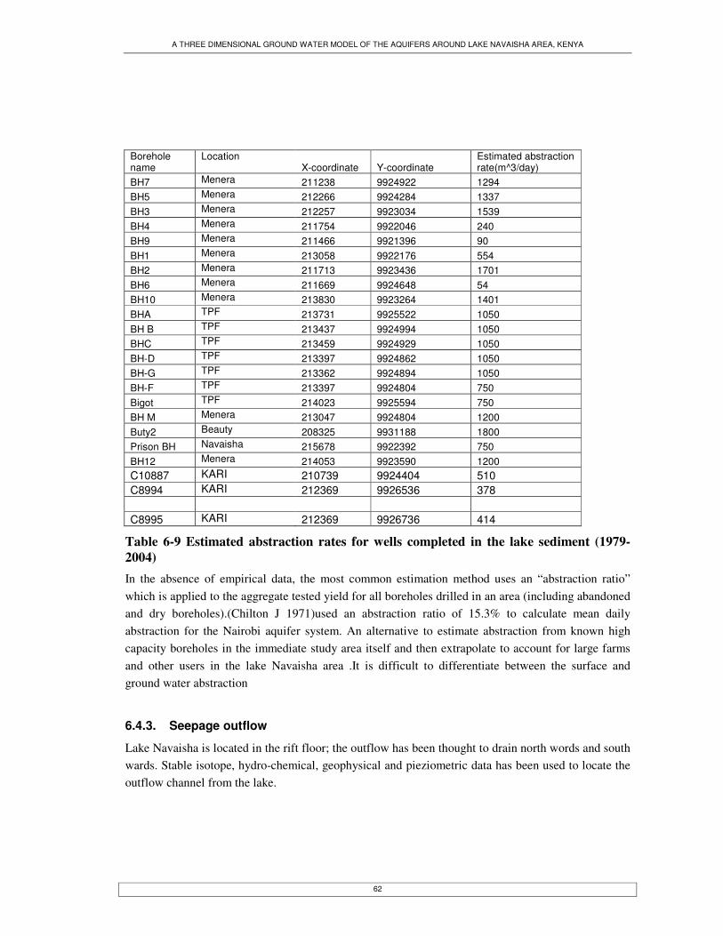
A THREE DIMENSIONAL GROUND WATER MODEL OF THE AQUIFERS AROUND LAKE NAVAISHA AREA, KENYA
62
Borehole name
Location X-coordinate Y-coordinate
Estimated abstraction rate(m^3/day)
BH7 Menera 211238 9924922 1294 BH5 Menera 212266 9924284 1337 BH3 Menera 212257 9923034 1539 BH4 Menera 211754 9922046 240 BH9 Menera 211466 9921396 90 BH1 Menera 213058 9922176 554 BH2 Menera 211713 9923436 1701 BH6 Menera 211669 9924648 54 BH10 Menera 213830 9923264 1401 BHA TPF 213731 9925522 1050 BH B TPF 213437 9924994 1050 BHC TPF 213459 9924929 1050 BH-D TPF 213397 9924862 1050 BH-G TPF 213362 9924894 1050 BH-F TPF 213397 9924804 750 Bigot TPF 214023 9925594 750 BH M Menera 213047 9924804 1200 Buty2 Beauty 208325 9931188 1800 Prison BH Navaisha 215678 9922392 750 BH12 Menera 214053 9923590 1200 C10887 KARI 210739 9924404 510 C8994 KARI 212369 9926536 378 C8995 KARI 212369 9926736 414
Table 6-9 Estimated abstraction rates for wells completed in the lake sediment (1979-2004) In the absence of empirical data, the most common estimation method uses an “abstraction ratio” which is applied to the aggregate tested yield for all boreholes drilled in an area (including abandoned and dry boreholes).(Chilton J 1971)used an abstraction ratio of 15.3% to calculate mean daily abstraction for the Nairobi aquifer system. An alternative to estimate abstraction from known high capacity boreholes in the immediate study area itself and then extrapolate to account for large farms and other users in the lake Navaisha area .It is difficult to differentiate between the surface and ground water abstraction
6.4.3. Seepage outflow
Lake Navaisha is located in the rift floor; the outflow has been thought to drain north words and south wards. Stable isotope, hydro-chemical, geophysical and pieziometric data has been used to locate the outflow channel from the lake.

A THREE DIMENSIONAL GROUND WATER MODEL OF THE AQUIFERS AROUND LAKE NAVAISHA AREA, KENYA
63
Figure 6-4 Analytical signal image of the study area (Tsiboah 2002)

A THREE DIMENSIONAL GROUND WATER MODEL OF THE AQUIFERS AROUND LAKE NAVAISHA AREA, KENYA
64
6.5. Selecting the model boundaries
A model boundary is the interface between the model calculation domain and the surrounding environment. In other words; the boundary condition is representative of unstressed ground water flow system. It is suggested that the entire regional be modelled in a steady state and the fluxes across the boundaries of the local model or site model (well fields) be applied to boundary of cells either as a general head boundary or flux boundaries depending on the regional steady state solution. The boundary conditions were defined as follows: Western part: The fault plane located at the foot of the Mau scarp was taken to be a no flow boundary. Most of the flow from this area has been inferred to be impeded by the fault associated with the Eburru volcanic complex to the west of the basin (trending north-south), and it disperses north-eastwards through the Eburru Hills and south-eastwards through the Olkaria region (Mcann 1974; Clarke A.C.G. 1990).What little finds its way into the lake is by deep percolation. There is no clear cut, exhaustive work in this area that definitely confirms this view. Considering that there is outflow from the lake through the Eburru complex area, it has been assumed reasonable enough to consider that, part of the flow from the Mau scarp gets to the lake. West side the fault is considered as a no flow boundary. Northern part: The north-eastern surface water divide is spanned by the Eburru hills beneath which are acknowledged to be outflow to the Elmentaita Lake basin (Darling et al., 1996). Due north of the basin, there is some outflow on its western fringe to the east of the Eburru Hills (Clarke A.C.G. 1990)and there is no physical boundary except the surface water shed which has no meaning with the groundwater. The boundary is located near lake Elmentata to show the continuity of the lake sediments, (which are intercepted by recent Eburru volcanics).The boundary was selected parallel to the ground water contour map as drawn by (Githae 1998) Eastern part: The South Kinangop fault trending due NNW is considered to impede most of the inflow from the Kinangop plateau. Most of the flux is considered to take place in the deeper horizons. Minimal flow through this area has been considered negligible since the East Faults scarps are proven fault by geological and composite image with evidence by comparable Electric conductivity (EC) value on both sides of the fault, indicating no ground water inflow. Besides the river direction are away from the fault. Indeed high hydraulic gradient is evident indicating low hydraulic conductivity which is coincidence of the fault in place. Southern part: Flow through the Olkaria and Longonot volcanic complexes has been considered to be the conduit for most of the lake outflow from the basin most of which percolates into the deeper geothermal systems. To the southeast of the Longonot volcano, some considerable outflow from the basin has been considered to account for the fluxes from the Kinangop plateau that gets into the basin in a south-westward direction. The basement and surface: The bottom of the system has been considered to be composed of undifferentiated volcanic materials that have a very low (Kzz<<Kxx≈Kyy) deep percolation of groundwater. This could also be attributed to the high pressures exerted by the deeper lying, highly volatile, multiphase geothermal systems that impede flow of water to the deeper horizons. It has been considered reasonable enough to be a no flow boundary over a long-term period. The solid model was used to define the elevation data of the model where the top considered as topographic land surface and the bottom of the basin corresponds to the elevations where the less permeable welded tuffs become dominant. Assigning two order magnitude of hydraulic conductance contrast is justified.The bottom of the flow domain ranges from 1479-1914 m.Indeed the solution of the flow problem with an impervious base at infinite depth is only a little different from the solution of the flow problem with an effective impervious base at finite depth(Ziji 1999).

A THREE DIMENSIONAL GROUND WATER MODEL OF THE AQUIFERS AROUND LAKE NAVAISHA AREA, KENYA
65
7. Numerical model
The need for groundwater management plans has necessitated the development of mathematical models to simulate groundwater flow, test aquifer parameters that characterize the ability of the aquifer to transmit and store water, and predict the response of the aquifer to groundwater pumping. The flow of fluids through media is governed by the laws of physics. As such it can be described by differential equations. Since the flow is a function of several variables, it is usually described by partial differential equations in which the spatial coordinates, x, y, z, and t, are the independent variables. In deriving the equations, the law of conservation for mass and energy are employed. Based upon these principles and Darcy’s law, the main equations of groundwater flow have been derived The partial-differential equation of ground-water flow used in MODFLOW is ((McDonald 1988)
th
SWzh
Kzy
hK
yxh
Kx szyx ∂
∂=−��
���
�
∂∂
∂∂+��
�
����
�
∂∂
∂∂+�
�
���
�
∂∂
∂∂ Equation 7-1
Where Kx, Ky, and Kz are values of hydraulic conductivity along the x, y, and z coordinate axes, which are assumed to be parallel to the major axes of hydraulic conductivity (L/T); h is the potentiometric head (L); W is a volumetric flux per unit volume representing sources and/or sinks of water, with W<0.0 for flow out of the ground-water system, and W>0.0 for flow in (T-1); SS is the specific storage of the porous material (L-1); and t is time (T). Equation 7.1 when combined with boundary and initial conditions, describes transient three-dimensional ground-water flow in a heterogeneous and anisotropic medium, provided that the principal axes of hydraulic conductivity are aligned with the coordinate directions. The Ground-Water Flow Process solves equation 5.1 using the finite-difference method in which the groundwater flow system is divided into a grid of cells (figure 7-2) For each cell, there is a single point, called a node, at which head is calculated. For steady-state stress periods, the storage term and, therefore, the right-hand side of equation 7.1 is set to zero.
7.1. Model design
MODFLOW-2000 (Harbaugh and others, 2000), which is a numerical, three-dimensional; finite-difference ground-water model was used to simulate flow in the aquifers including packages. These packages includes Layer-Property Flow, River, Recharge, Well, Drain, and Evapo-transpiration.
7.1.1. Discretization and Representation of the Hydro-geologic Framework
In numerical model, the continuous domain is replaced by a discretized domain, which consists of an array of nodes and associated finite difference blocks or finite element (Anderson M.P. 1992).A fundamental aspect of numerical models is the representation of the real world by discrete volumes of material. The accuracy of the model is limited by the size of the discrete volumes. Grid size depends on hydraulic gradient, scale of aquifer heterogeneity, size of the modelled area, level of detail for the solution of the problem. Selecting size of the node is critical step in grid design .The size of nodal spacing in the horizontal dimension is function of expected curvature in the water table. A grid with smaller number of nodes is preferred in order to minimize data handling, computer storage and computation time. But it needs large number of nodes to represent the system accurately. The need to select meaningful boundaries may require modelling a large area. A telescopic mesh refinement
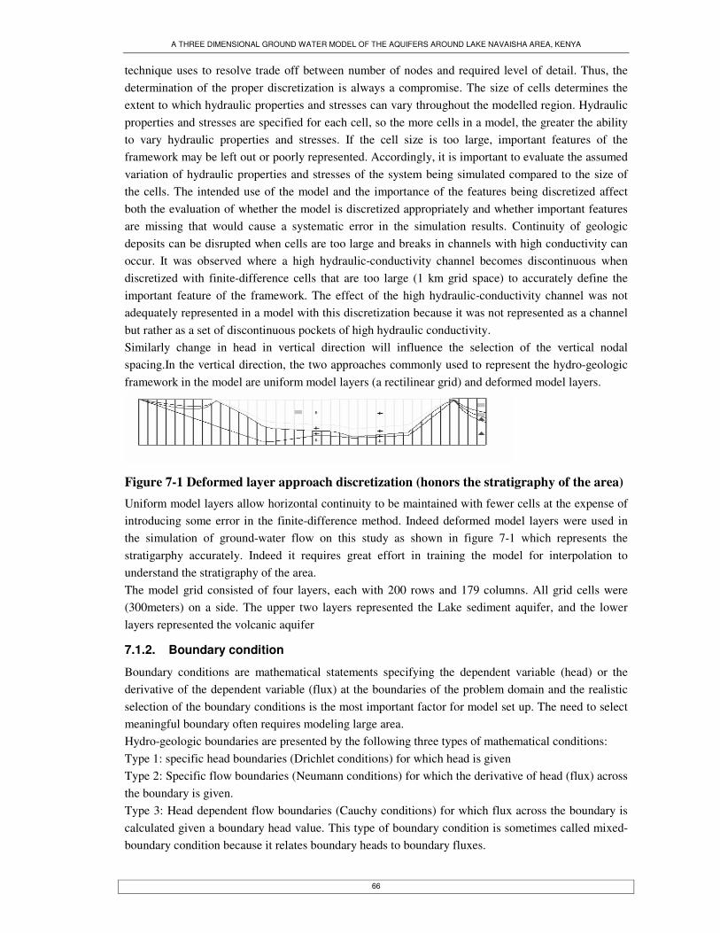
A THREE DIMENSIONAL GROUND WATER MODEL OF THE AQUIFERS AROUND LAKE NAVAISHA AREA, KENYA
66
technique uses to resolve trade off between number of nodes and required level of detail. Thus, the determination of the proper discretization is always a compromise. The size of cells determines the extent to which hydraulic properties and stresses can vary throughout the modelled region. Hydraulic properties and stresses are specified for each cell, so the more cells in a model, the greater the ability to vary hydraulic properties and stresses. If the cell size is too large, important features of the framework may be left out or poorly represented. Accordingly, it is important to evaluate the assumed variation of hydraulic properties and stresses of the system being simulated compared to the size of the cells. The intended use of the model and the importance of the features being discretized affect both the evaluation of whether the model is discretized appropriately and whether important features are missing that would cause a systematic error in the simulation results. Continuity of geologic deposits can be disrupted when cells are too large and breaks in channels with high conductivity can occur. It was observed where a high hydraulic-conductivity channel becomes discontinuous when discretized with finite-difference cells that are too large (1 km grid space) to accurately define the important feature of the framework. The effect of the high hydraulic-conductivity channel was not adequately represented in a model with this discretization because it was not represented as a channel but rather as a set of discontinuous pockets of high hydraulic conductivity. Similarly change in head in vertical direction will influence the selection of the vertical nodal spacing.In the vertical direction, the two approaches commonly used to represent the hydro-geologic framework in the model are uniform model layers (a rectilinear grid) and deformed model layers.
Figure 7-1 Deformed layer approach discretization (honors the stratigraphy of the area) Uniform model layers allow horizontal continuity to be maintained with fewer cells at the expense of introducing some error in the finite-difference method. Indeed deformed model layers were used in the simulation of ground-water flow on this study as shown in figure 7-1 which represents the stratigarphy accurately. Indeed it requires great effort in training the model for interpolation to understand the stratigraphy of the area. The model grid consisted of four layers, each with 200 rows and 179 columns. All grid cells were (300meters) on a side. The upper two layers represented the Lake sediment aquifer, and the lower layers represented the volcanic aquifer
7.1.2. Boundary condition
Boundary conditions are mathematical statements specifying the dependent variable (head) or the derivative of the dependent variable (flux) at the boundaries of the problem domain and the realistic selection of the boundary conditions is the most important factor for model set up. The need to select meaningful boundary often requires modeling large area. Hydro-geologic boundaries are presented by the following three types of mathematical conditions: Type 1: specific head boundaries (Drichlet conditions) for which head is given Type 2: Specific flow boundaries (Neumann conditions) for which the derivative of head (flux) across the boundary is given. Type 3: Head dependent flow boundaries (Cauchy conditions) for which flux across the boundary is calculated given a boundary head value. This type of boundary condition is sometimes called mixed-boundary condition because it relates boundary heads to boundary fluxes.

A THREE DIMENSIONAL GROUND WATER MODEL OF THE AQUIFERS AROUND LAKE NAVAISHA AREA, KENYA
67
A general head boundary (GHB) package was employed to simulate head dependent flow boundaries. Flow across the boundaries is calculated using the expression Qb=Cb*(hb-h) Where Cb is the hydraulic conductance (m2/day) hb is the hydraulic head at the boundary(m) H is the hydraulic head in the aquifer (m) The General Head package is similar to the river and drain packages in that flow in or out of a cell is proportional to a difference in head. General head conditions are specified by assigning a head and a conductance to a selected set of cells. If the water table elevation rises above the specified head, water flows out of the aquifer. If the water table elevation falls below the specified head, water flows into the aquifer. In both cases, the flow rate is proportional to the head difference and the constant of proportionality is the conductance. General Head Boundary is preferable than constant head since it allows to change the head and conductance value at different stress periods. Also it minimizes constraining the model. Outer pieziometeric data were used to define general head boundary condition together with cells nodes representing measured wells with GPS(Garmin summit eterix with vertical resolution 10ft) (figure 7-2).The interpolation method of head value is shown in appendix 8. Cells of constant hydraulic head were used to spring points on the eastern model boundary.
Figure 7-2 wells (and springs) heads used for assigning specific head nodes.

A THREE DIMENSIONAL GROUND WATER MODEL OF THE AQUIFERS AROUND LAKE NAVAISHA AREA, KENYA
68
All boundaries were designated as “general head,” where the northern model boundary was delineated approximately parallel to the estimated ground-water contour line. (See appendix 7 showing the ground water contour prepared by (Githae 1998)
7.2. Initial Conditions
The initial conditions describe the distribution of the heads throughout the model domain at the start of the simulation. The initial conditions have been considered to be the hydrologic stresses (lake levels, river flows) at the 1932 period. However, the initial groundwater levels have been derived as a long-term average value from 1932 to 1998 interpolated within the model to obtain the initial piezometric surface. This was so done because (1) levels within this duration correspond to the natural stresses that were acting in the system then, (2) lack of enough data to adequately describe the piezometric surface at the start of the simulation period. The initial conditions for the steady state simulation are important mainly to save computational effort in reaching a solution. However, the initial conditions for a transient problem strongly influence the predicted results. Moreover use of model generated head values ensures that the initial head data and the model hydrologic inputs and parameters are consistent (Franke 1987).
7.3. Representation of hydraulic properties
Estimated horizontal hydraulic conductivity for the surfacial aquifer (layer1) ranged from 0.01-850 m/day(Appendix 4) and from 0.2 to 1183 metres per day for layer 2(Appendix 5) Estimated values were based on previously published values represented as pilot points. The spatial distribution of horizontal hydraulic conductivity estimated by (Clarke 1990) is in general agreement with that shown in figure7-3. Initial estimates were derived from Table 6-1,6-3 and 6-4.Estimated horizontal hydraulic conductivity for the volcanic aquifer ranged from 0.05 to 10 metres per day. Zones of a higher horizontal hydraulic conductivity were assigned along the fracture/fault zone in order to calibrate to the substantial ground-water outflow that occurs to southern and northern of lake Navaisha, based on isotopic, hydro-chemical, geological, geophysical and pieziometric evidences. In addition, if the locations of these streams (namely, Gilgil and Karati river) are influenced by fractures or faults, higher hydraulic conductivity could result. Previously published values were used as general indicators for hydraulic conductivity values and distributions; however, model calibration carried the
most weight in determining the final values and distributions.In GMS hydraulic properties can be assigned either as data array or material identity. In this study the hydraulic properties was assigned based on data array to better represent the fracture flow by representing in the faults/fractures in the map coverage .Meanwhile, the zonation was applied based on the discretized hydro-geological units. Therefore, the calibration accuracy obtained using the larger zones shown in figures 7-3 and 7-4 was considered sufficient to fulfil the objectives of this study.
Figure 7-3 Zonation of horizontal hydraulic conductivity of the sediment aquifer (Where the lake Elementata is represented by polygon in the upper most of the figure and the line represents the Navaisha watershed boundary.) Zone delineation for hydraulic properties of volcanic aquifer was determined by considering potential structural features
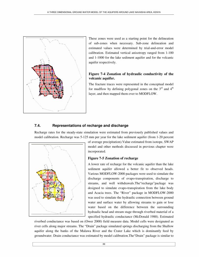
A THREE DIMENSIONAL GROUND WATER MODEL OF THE AQUIFERS AROUND LAKE NAVAISHA AREA, KENYA
69
These zones were used as a starting point for the delineation of sub-zones when necessary. Sub-zone delineation and estimated values were determined by trial-and-error model calibration. Estimated vertical anisotropy ranged from 1-100 and 1-1000 for the lake sediment aquifer and for the volcanic aquifer respectively.
Figure 7-4 Zonation of hydraulic conductivity of the volcanic aquifer. The fracture traces were represented in the conceptual model for mudflow by defining polygonal zones on the 3rd and 4th layer, and then mapped them over to MODFLOW.
7.4. Representations of recharge and discharge
Recharge rates for the steady-state simulation were estimated from previously published values and model calibration. Recharge was 5-125 mm per year for the lake sediment aquifer (from 1-20 percent
of average precipitation).Value estimated from isotope, SWAP model and other methods discussed in previous chapter were incorporated.
Figure 7-5 Zonation of recharge A lower rate of recharge for the volcanic aquifer than the lake sediment aquifer allowed a better fit to observed heads. Various MODFLOW-2000 packages were used to simulate the discharge components of evapo-transpiration, discharge to streams, and well withdrawals.The“recharge”package was designed to simulate evapo-transpiration from the lake body and Acacia trees. The “River” package in MODFLOW-2000 was used to simulate the hydraulic connection between ground water and surface water by allowing streams to gain or lose water based on the difference between the surrounding hydraulic head and stream stage through riverbed material of a specified hydraulic conductance (McDonald 1988). Estimated
riverbed conductance was based on (Ower 2000) field measure data. Model cells were designated as river cells along major streams. The “Drain” package simulated springs discharging from the Shallow aquifer along the banks of the Malawa River and the Crater Lake which is dominantly feed by groundwater. Drain conductance was estimated by model calibration.The“Drain” package is similar to
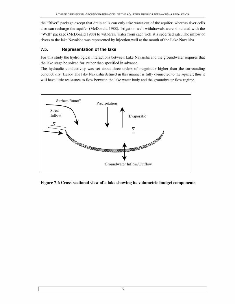
A THREE DIMENSIONAL GROUND WATER MODEL OF THE AQUIFERS AROUND LAKE NAVAISHA AREA, KENYA
70
the “River” package except that drain cells can only take water out of the aquifer, whereas river cells also can recharge the aquifer (McDonald 1988). Irrigation well withdrawals were simulated with the “Well” package (McDonald 1988) to withdraw water from each well at a specified rate. The inflow of rivers to the lake Navaisha was represented by injection well at the mouth of the Lake Navaisha.
7.5. Representation of the lake
For this study the hydrological interactions between Lake Navaisha and the groundwater requires that the lake stage be solved for, rather than specified in advance. The hydraulic conductivity was set about three orders of magnitude higher than the surrounding conductivity. Hence The lake Navaisha defined in this manner is fully connected to the aquifer; thus it will have little resistance to flow between the lake water body and the groundwater flow regime.
Figure 7-6 Cross-sectional view of a lake showing its volumetric budget components
=
Evaporatio
Precipitation
StreaInflow
Surface Runoff
Groundwater Inflow/Outflow
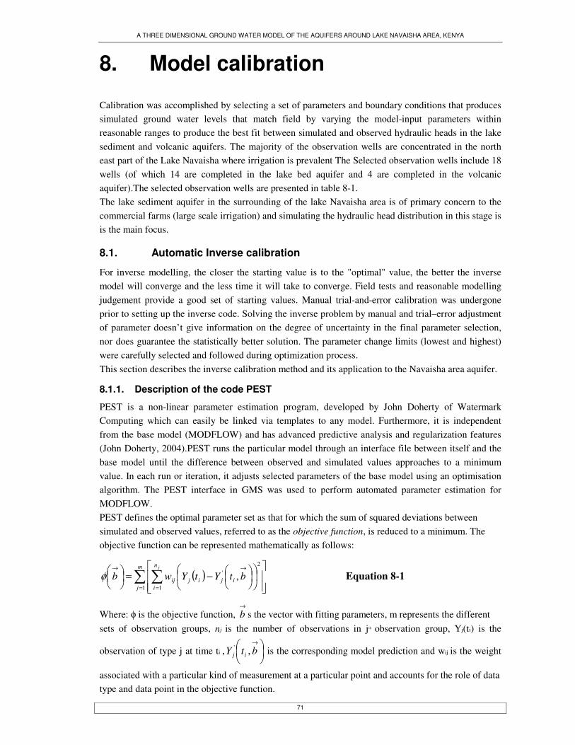
A THREE DIMENSIONAL GROUND WATER MODEL OF THE AQUIFERS AROUND LAKE NAVAISHA AREA, KENYA
71
8. Model calibration
Calibration was accomplished by selecting a set of parameters and boundary conditions that produces simulated ground water levels that match field by varying the model-input parameters within reasonable ranges to produce the best fit between simulated and observed hydraulic heads in the lake sediment and volcanic aquifers. The majority of the observation wells are concentrated in the north east part of the Lake Navaisha where irrigation is prevalent The Selected observation wells include 18 wells (of which 14 are completed in the lake bed aquifer and 4 are completed in the volcanic aquifer).The selected observation wells are presented in table 8-1. The lake sediment aquifer in the surrounding of the lake Navaisha area is of primary concern to the commercial farms (large scale irrigation) and simulating the hydraulic head distribution in this stage is is the main focus.
8.1. Automatic Inverse calibration
For inverse modelling, the closer the starting value is to the "optimal" value, the better the inverse model will converge and the less time it will take to converge. Field tests and reasonable modelling judgement provide a good set of starting values. Manual trial-and-error calibration was undergone prior to setting up the inverse code. Solving the inverse problem by manual and trial–error adjustment of parameter doesn’t give information on the degree of uncertainty in the final parameter selection, nor does guarantee the statistically better solution. The parameter change limits (lowest and highest) were carefully selected and followed during optimization process. This section describes the inverse calibration method and its application to the Navaisha area aquifer.
8.1.1. Description of the code PEST
PEST is a non-linear parameter estimation program, developed by John Doherty of Watermark Computing which can easily be linked via templates to any model. Furthermore, it is independent from the base model (MODFLOW) and has advanced predictive analysis and regularization features (John Doherty, 2004).PEST runs the particular model through an interface file between itself and the base model until the difference between observed and simulated values approaches to a minimum value. In each run or iteration, it adjusts selected parameters of the base model using an optimisation algorithm. The PEST interface in GMS was used to perform automated parameter estimation for MODFLOW. PEST defines the optimal parameter set as that for which the sum of squared deviations between simulated and observed values, referred to as the objective function, is reduced to a minimum. The objective function can be represented mathematically as follows:
( )� �= =
→→
��
���
��
���
���
���
�−=��
���
� m
j
n
iijijij
j
btYtYwb1 1
2' ,φ Equation 8-1
Where: φ is the objective function, →b s the vector with fitting parameters, m represents the different
sets of observation groups, nj is the number of observations in jth observation group, Yj(ti) is the
observation of type j at time ti , ��
���
� →btY ij ,' is the corresponding model prediction and wij is the weight
associated with a particular kind of measurement at a particular point and accounts for the role of data type and data point in the objective function.
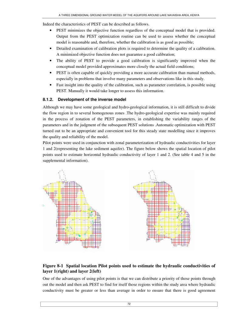
A THREE DIMENSIONAL GROUND WATER MODEL OF THE AQUIFERS AROUND LAKE NAVAISHA AREA, KENYA
72
Indeed the characteristics of PEST can be described as follows. • PEST minimizes the objective function regardless of the conceptual model that is provided.
Output from the PEST optimization routine can be used to assess whether the conceptual model is reasonable and, therefore, whether the calibration is as good as possible;
• Detailed examination of calibration plots is required to determine the quality of a calibration. A minimized objective function does not guarantee a good calibration;
• The ability of PEST to provide a good calibration is significantly improved when the conceptual model provided approximates more closely the actual field conditions;
• PEST is often capable of quickly providing a more accurate calibration than manual methods, especially in problems that involve many parameters and observations like in this study.
• Fast insight into the quality of the calibration, such as parameter correlation, is possible using PEST. Manually it would take longer to assess this information.
8.1.2. Development of the inverse model
Although we may have some geological and hydro-geological information, it is still difficult to divide the flow region in to several homogenous zones .The hydro-geological expertise was mainly required in the process of zonation of the PEST parameters, in establishing the variability ranges of the parameters and in the judgment of the subsequent PEST solutions .Automatic optimization with PEST turned out to be an appropriate and convenient tool for this steady state modelling since it improves the quality and reliability of the model. Pilot points were used in conjunction with zonal parameterization of hydraulic conductivities for layer 1 and 2(representing the lake sediment aquifer). The figure below shows the spatial location of pilot points used to estimate horizontal hydraulic conductivity of layer 1 and 2. (See table 4 and 5 in the supplemental information).
Figure 8-1 Spatial location Pilot points used to estimate the hydraulic conductivities of layer 1(right) and layer 2(left) One of the advantages of using pilot points is that we can distribute a priority of those points through out the model and then ask PEST to find for itself those regions within the study area where hydraulic conductivity must be greater or less than average in order to ensure that there is good agreement

A THREE DIMENSIONAL GROUND WATER MODEL OF THE AQUIFERS AROUND LAKE NAVAISHA AREA, KENYA
73
between model output and field measurements. Parameterization is the process of selecting input values, and grouping them into parameter sets to reduce the number of independent parameters. In order to ensure that the parameter estimation process is stable, regularization was used in conjunction with PEST. The introduction of regularisation into the calibration process serves two purposes. Firstly it brings a high degree of numerical stability to a parameter estimation problem which would otherwise be highly susceptible to the deleterious effects of a singular normal matrix (was not able to calculate any parameter statistics due to singularity of the normal matrix.) Secondly, if regularisation constraints are appropriately defined, model calibration can proceed, in spite of the number of parameters at its disposal. Regularization is a way of alleviating the ill-posedness of the inverse problem through incorporation of prior information in to objective function (Richard C. Aster 2003)
8.1.3. Inverse calibration results
Calibration was accomplished by selecting a set of parameters, boundary conditions and stresses that produces simulated ground water levels that match field evidence. The whole procedure was done with in pre established calibration target. A Maximum 10m as an acceptable difference between computed and simulated head for deep gradient near escarpment and a target of 1m for the floor of the basin. As a result levelled wells are useful for this purpose. The hydraulic conductivity value of layer 1 was adjusted and spatially discretized further based on the drainage density, fracture density and prior information by maintaining the relationship between the hydro-geological unit and hydraulic conductivity zonation.Estimate of hydraulic values obtained from field investigations are used as pilot points.
Hydraulic heads and Potentiometric surfaces
Calibration criteria for the steady-state simulation included :(1) generally matching the simulated potentiometric surfaces and hydraulic gradients to those of the estimated potentiometric surfaces, and (2) matching hydraulic heads. The Mean residuals for 15 of these observations wells were within ±1.3 metres. The RMSE (root Mean squared residual) and MAR (Mean Absolute Residual) were 3 and 1.8 m respectively.
Figure 8-2 Computed versus observed head value for the selected observation wells The calibration target in the steady state model was to match heads calculated by the model with the measured head points. Some of the observation wells were measured using Garmin eterix summit

A THREE DIMENSIONAL GROUND WATER MODEL OF THE AQUIFERS AROUND LAKE NAVAISHA AREA, KENYA
74
GPS, with 3m metres accuracy. Thus, more weight was given to those wells which are accurately levelled because of a higher degree of confidence in that data. The average of differences was used to quantify the average error in the calibration. The residual head helps to visualize where error prone parameters are. Mean while the observation wells located along the Eburru (EW 1) and two other wells located in the southern part of the study area are considered as outliers. A listing of measured and simulated heads together with their differences are shown in table 8-1.
Bore hole no UTM_X UTM_Y
Observed head elevation(m)
Computed head elevation(m)
Head difference (m)
Used for aquifer type
ITC040 201591 9926461 1885 1885.78 -0.78 Sedimentary ITC042 207165 9925364 1886 1885.12 +0.88 Sedimentary ITC082 206306 9931350 1886 1887 -1 Sedimentary ITC107 212412 9903826 1899 1898.45 -0.55 Sedimentary ITC149 217150 9918100 1929 1928.6 +0.4 Sedimentary ITC161 197660 9918954 1888 1888.67 -0.33 Sedimentary ITC180 203360 9925256 1886 1885 +1 Sedimentary
ITC183 208323 9931189 1884 1884.92 -.08 Volcanic
N40 216441 9913361 1910 1914 -4 Sedimentary C2709 186474 9907789 2114 2112.6 +1.4 Sedimentary C1404 190190 9915161 1894 1893 +1 Sedimentary C2300 190500 9909750 1914 1911.12 +2.88 Sedimentary
EW1 196900 9930575 1852 1871
-21 Volcanic
C2586 198500 9905140 1842 1841 +1 Volcanic
C733 202750 9940250 1819 1827
-8
Volcanic
ITC_ked1 214204 9907097 1904 1903.12
+0.88
Sedimentary
ITC_sher 208867 9909074 1883 1883.74 -0.74 Sedimentary Lake_1 203610 9914710 1887.68 1888.74 -0.06 Lake Lake_2 199030 9914360 1887.68 1888.75 -0.07 Lake Lake_3 206550 9914770 1887.68 1888.74 -0.06 Lake Lake_4 209010 9914910 1888.68 1888.74 -0.06 Lake
Table 8-1 A lists of observed and simulated heads together with their differences for the selected wells The computed vs. observed values were displayed using” calibration targets" displayed at each observation well. The size, direction, and color of the bars on the targets (shown in figure 8-3 and 8-4) provide feedback on the magnitude and spatial distribution of the observation error. Most importantly, they provide feedback at precisely the locations that the measurements were taken.
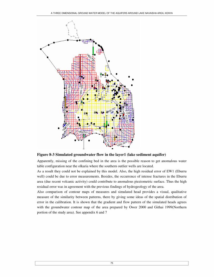
A THREE DIMENSIONAL GROUND WATER MODEL OF THE AQUIFERS AROUND LAKE NAVAISHA AREA, KENYA
75
Figure 8-3 Simulated groundwater flow in the layer1 (lake sediment aquifer) Apparently, missing of the confining bed in the area is the possible reason to get anomalous water table configuration near the olkaria where the southern outlier wells are located. As a result they could not be explained by this model. Also, the high residual error of EW1 (Eburru well) could be due to error measurements. Besides, the occurrence of intense fractures in the Eburru area (due recent volcanic activity) could contribute to anomalous pieziometric surface. Thus the high residual error was in agreement with the previous findings of hydrogeology of the area. Also comparison of contour maps of measures and simulated head provides a visual, qualitative measure of the similarity between patterns, there by giving some ideas of the spatial distribution of error in the calibration. It is shown that the gradient and flow pattern of the simulated heads agrees with the groundwater contour map of the area prepared by Ower 2000 and Githai 1999(Northern portion of the study area). See appendix 6 and 7
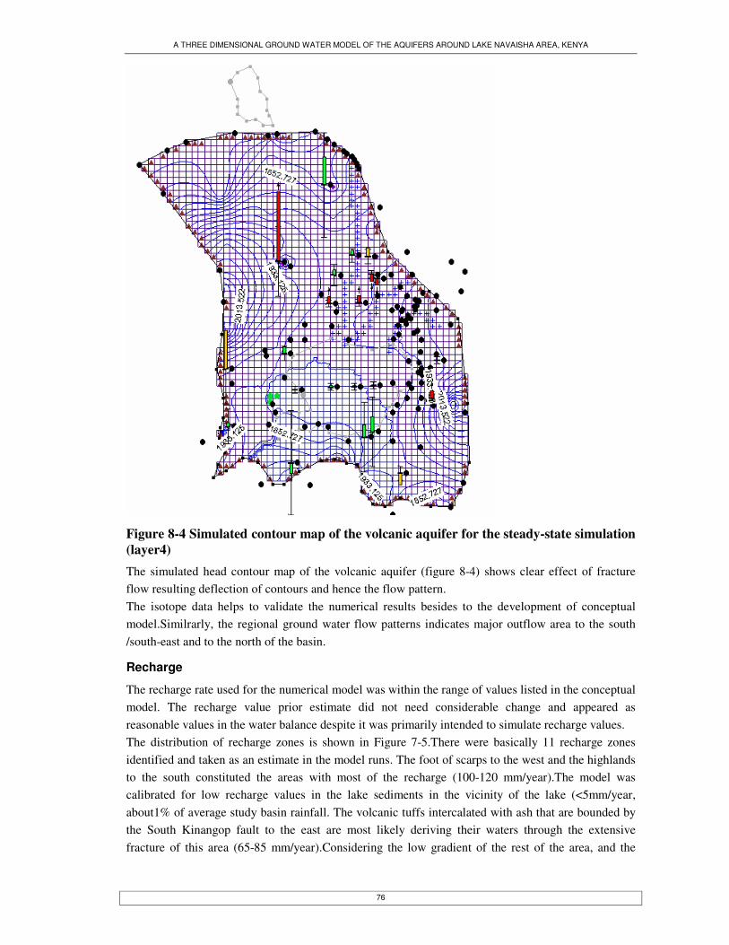
A THREE DIMENSIONAL GROUND WATER MODEL OF THE AQUIFERS AROUND LAKE NAVAISHA AREA, KENYA
76
Figure 8-4 Simulated contour map of the volcanic aquifer for the steady-state simulation (layer4) The simulated head contour map of the volcanic aquifer (figure 8-4) shows clear effect of fracture flow resulting deflection of contours and hence the flow pattern. The isotope data helps to validate the numerical results besides to the development of conceptual model.Similrarly, the regional ground water flow patterns indicates major outflow area to the south /south-east and to the north of the basin.
Recharge
The recharge rate used for the numerical model was within the range of values listed in the conceptual model. The recharge value prior estimate did not need considerable change and appeared as reasonable values in the water balance despite it was primarily intended to simulate recharge values. The distribution of recharge zones is shown in Figure 7-5.There were basically 11 recharge zones identified and taken as an estimate in the model runs. The foot of scarps to the west and the highlands to the south constituted the areas with most of the recharge (100-120 mm/year).The model was calibrated for low recharge values in the lake sediments in the vicinity of the lake (<5mm/year, about1% of average study basin rainfall. The volcanic tuffs intercalated with ash that are bounded by the South Kinangop fault to the east are most likely deriving their waters through the extensive fracture of this area (65-85 mm/year).Considering the low gradient of the rest of the area, and the
A THREE DIMENSIONAL GROUND WATER MODEL OF THE AQUIFERS AROUND LAKE NAVAISHA AREA, KENYA
77
mixture of sediments and reworked volcanic material that underlie it, the quantity of recharge here is also quite sizeable (20-25 mm/year).
Hydraulic conductivity
These parameters were identified for zones of the model that were determined before the calibration process (a priori).Parameter zones for hydraulic conductivity is shown in figure 7-3 and 7-4 for the layers of a model. The areal extent of these units remains fixed during automatic calibration, and the conceptualization of the location and extent of these zones was part of the information specified before the automatic calibration process. Optimized Hydraulic conductivity values range between 0.0001 to1500m/day.Areas with high hydraulic conductivity values coincides with mapped and inferred lineament intersections. During calibration initial estimated hydraulic conductivities were reduced to achieve a match between measured and simulated heads. Those changes were justified because lower hydraulic conductivities are typically observed in the low fracture density area. The area located near to the general head boundary cannot be considered calibrated because of the close proximity of the calibration points to the specific head boundary.
8.1.4. Calibration result evaluation
The results of the calibration were evaluated both qualitatively and quantitatively. The calibration targets were hydraulic head, hydraulic head gradient, and fluxes. The mass balance of water into and out of the system had minimal error. The steady state calibration was evaluated based on: 1. Most of the simulated heads were with in pre-established calibration target, a max 10m as an acceptable difference between and simulated head for deep gradient near escarpment and 1m for the floor of the basin together with the ground water balance of the area. Possible explanation was given for the outlier wells. 2. Water balance was near to 0. (It was 0.02%) 3. Simulated aerial distribution ET matched the estimated distribution (simulated ET was 0.0047 m/day). 4. Whether the error or residual was random. Besides to the quantitative measures that were used to show the accuracy of the calibration of a ground-water flow model, the areal distribution of residuals (differences between measured and simulated values) also was important to determine whether some areas of the model are biased either too high or too low. A scatter plot of measured against simulated heads is another way of showing the calibrated fit. Deviation of points from the straight line should be randomly distributed. At first, the model was recalibrated again due to systematic error. Eventually, the scatter plot showed a reasonable fit and points in the straight line were randomly distributed and an explanation was given for the outlier wells (Figure 8-2). Overall, the finite difference groundwater model result was comparable with measured well data and with the isotope and hydro-chemical data interpretations.
8.2. Sensitivity analysis
Sensitivity analysis is the evaluation of model input parameters to see how much they affect model outputs (in this cases heads). The relative effect of the parameters helps to provide fundamental understanding of the simulated system. Sensitivity analysis also is inherently part of model calibration. The most sensitive parameters will be the most important parameters for causing the model to match observed values. Sensitivity analysis can be conducted manually or automatically.

A THREE DIMENSIONAL GROUND WATER MODEL OF THE AQUIFERS AROUND LAKE NAVAISHA AREA, KENYA
78
The automatic approach directly computes parameter sensitivity. Automatic sensitivity analysis is inherently part of automatic parameter adjustment for model calibration.The automatic parameter adjustment algorithm uses parameter sensitivity to compute the parameter values that cause the model to best match observed heads. Regularization does this by introducing the regularization constraints to the parameter estimation process. In other words, the statistics of parameter sensitivities, observation sensitivities and residual are not really suitable for use after a regularized inversion run (except as a check that regularization did in fact bring numerical stability to the process by reducing the range of sensitivities and the ratio of highest to lowest eigen value thereby reducing the condition number of the matrix which PEST must invert in order to calculate parameter estimates). Normally, after a non-regularization run, it is good to look at sensitivities and parameter uncertainties. However after a run involving regularization, things are a little different, for the aim of regularization is to equalize sensitivities and reduce parameter uncertainty. (Also,” uncertainty" must be calculated differently).Meanwhile, there are some good reference in the book of (Richard C. Aster 2003) on how to post process a regularization run. However this has not been done yet in the ground water context because the software isn't available yet. (Personal communication with John Doherty, PEST developer, Australia).The concept of resolution is an important way to characterize the bias of the generalized inverse solution after regularization run. In this approach we see how closely the generalized inverse solution matches a given model. Meanwhile these references may give something to think about for further post processing of the regularization runs. In this study, a sensitivity analysis was used manually to examine the response of the numerical model calibrated to the steady-state condition to changes in model parameters, namely horizontal hydraulic conductivity, of the lake and aquifer by holding other parameters fixed to test the sensitivity of the calculated lake level to the value of hydraulic conductivity used to represent the lake (K2) relative to the aquifer (K1). More important, the large areal extent of the model allowed the examination of examine hydrological features not included in the previous models, resulting in new insights about the effects that far-field boundary conditions can have on near-field model calibration and parameterization. Meanwhile six observation wells were employed to define the regional gradient. Similarly 4 observation wells are located along the lake surface to evaluate the gradient of the across the lake. In the first set of simulation, the gradient across the model was equal to 1.48*10-3 m/m, but K2/K1 was increased successively from 10 to 1*107.For large values of K2/K1, a smaller convergence criterion and a larger number of iteration s were required to produce comparable accuracy in the mass balance (table 8-2) where a simulation with K2/K1 equal to 1*104 and a convergence criteria of .01 produced a mass balance error on the order of 0.08%.
Table 8-2 Results for the simulation K2 is the hydraulic conductivity assigned to the lake nodes and K1 is the hydraulic conductivity of the aquifer; K1 was set to 5 m/day in all simulations.
K2/K1 Lake level at centre
Convergence criterion
Mass balance error (%)
Number of iterations
Head drop across the Lake(m)
10 1881 0.65 0.38 23 0.25 100 1884 0.35 0.2 58 0.11 1000 1887.5 0.1 0.01 67 0.04 10000 1888.89 0.01 0.04 94 0.01 100000 1889.32 0.001 0.08 145 0.001 10000000 - 0.0001 - 245 Not converged

A THREE DIMENSIONAL GROUND WATER MODEL OF THE AQUIFERS AROUND LAKE NAVAISHA AREA, KENYA
79
A valid solution should also produce a constant water level across the lake. The solution for a simulation in which K2/K1 was equal to 10,000 produced an acceptable solution (figure 8-6) with the head drop across the lake equal to 0.01m (Table 8-2) and the hydraulic gradient across the lake equal to 1.55*10-5 m/m. Additional steady state simulation was performed to explore the relation ship between K2/K1 and the regional gradient imposed by the boundary conditions In the second series of the steady state simulations, the conductance value of the general head boundary was decreased in 1/10 and 1/100 of the optimized values to produce higher regional gradients to determine whether the regional gradient influences the choice of an appropriate value for K2/K1 in the high K solution. In the second series of simulation designed to test the effect of the regional gradient, It was found that solutions with K2/K1 equal to 1000 were, more sensitive to regional gradient than were solutions using K2/k1 equal to 10,000(Figure 8-6), although both sets of solutions gave the same lake level at a node near the centre of the lake. These results suggest for this problem, the best choice of K2/K1 is 10,000, with the convergence criterion equal to 1*10 -2 m.
0
0.00002
0.00004
0.00006
0.00008
0.0001
0.00012
0.00014
0.00016
0 0.001 0.002 0.003 0.004Regional gradient(m/m)
Gra
dien
t acr
oss
lake
(m/m
) K2/K1=100K2/K1=10000
Figure 8-5 Effect of regional gradient and value of K2/K1 on the calculated hydraulic gradient across the lake The convergence criteria was set to 0.65 m for the solutions with K2/K1=100 and 0.01m for the solutions with K2/K1=10,000. The ratio of the hydraulic gradient across the lake to the regional gradient clearly indicates whether the gradient across the lake is close enough to zero. In previous application of the high–K method workers have used K2/K1 equal to 1000 with regional gradient on the order of 0.001m/m(Hunt.R.J. 1996) or 0.01m/m(Lee 1996). Therefore, higher values of K2/K1 should be used with higher regional gradients to ensure accurate calculations of seepage rates to and from the lake. From this sensitive analysis useful guide line for assessing the accuracy of the solution is to require that the ratio of the hydraulic gradient across the lake to the regional gradient be less than 0.001.
A THREE DIMENSIONAL GROUND WATER MODEL OF THE AQUIFERS AROUND LAKE NAVAISHA AREA, KENYA
80
8.3. Regional to local model conversion
For many modelling studies, determining an appropriate set of boundary conditions can be difficult. It is often the case that classical boundaries such as rock outcroppings, rivers, lakes, and groundwater divides, may be located at a great distance from the site of interest. In such cases, it is often convenient to perform the modelling study in two phases. In the first phase, a large, regional scale model was constructed .During the second stage, a second, smaller, local scale model was constructed that occupies a small area within the regional model. The groundwater elevations computed from the regional model are applied as specified head boundary conditions to the local scale model. The layer data, including elevations and hydraulic conductivities, were also interpolated from the regional to the local model. A more detailed representation of the local flow conditions, including low capacity wells and barriers not included in the regional flow model can be constructed in the local scale model. Regional to local model conversion is often referred to as “telescopic grid refinement."
8.3.1. Description of the problem
The site of interest is situated in the north east of the regional model which corresponds to commercial farms with large scale irrigation while the rest of the basin is more or less under natural condition. Once the regional model was completed, a local scale model is to be developed and then used to analyze a number of extraction well placement scenarios. A regional model was constructed for a large area. The steady state solution of the regional model was used to set boundary conditions for the steady state at the local scale. This model has four layers and similar zone of conductivity. As before, the western, eastern and southern coincided with the fault line. The northern boundaries were specified as a general head boundary taken from a solution of the regional model. The steady state solution of the regional model was used to set boundary conditions for the steady state at the local scale.The basic goal of the regional to local model conversion process was to create a 2D scatter point set containing the heads and layer data arrays from the regional model, create the local model, and interpolate the heads and layer data to the local model. A 2D scatter point set was used since the MODFLOW arrays should be interpolated on a layer by layer basis using 2D interpolation. The basic steps were as follows: 1. Generate the regional model and compute a solution. 2. Convert the MODFLOW Layers to 2-D Scatter Points, to create the scatter point set with the layer and head data from the regional model. 3. Create the 3-D grid for the local scale model. 4. Interpolate the heads and layer data values from the scatter points to the MODFLOW layer arrays for the local scale model. The boundary of the local and site model were shown in figure 8-6 and in Figure 8-7(indicated with a rectangle) shown respectively. These models were constructed using the conceptual model approach.

A THREE DIMENSIONAL GROUND WATER MODEL OF THE AQUIFERS AROUND LAKE NAVAISHA AREA, KENYA
81
Figure 8-6 Local model The effect of the boundary conditions on the solution was evaluated by changing specific head conditions to specific flow and vice versa. According to (de Marsily 1986)the boundary does not affect the solution if the resulting changes in the head solution are insignificant. Indeed it was found that the stress imposed on the system during the simulation propagated out to the boundary of the local modelled system and caused a simulated effect that was unrealistic.
Figure 8-7 Site model (well field area) uncertainties to the ground water distribution due to presence of trachyte ridges and obsidian lava flows could be better minimized at site model using the detail geophysical interpretation of the well fields done by (Tsiboah 2002).Meanwhile, the boundaries of the site model was marked as specified head boundaries using the computed head values from the regional model. A rectangular grid was constructed where two opposite boundaries were parallel to head contours from the regional model (i.e. a constant head value along each boundary).The other two boundaries were no flow boundaries and are perpendicular to the head contours from the regional model with aerial grid space 80 m on side.Effort was made to set boundary condition for a site model (at the commercial farms) from solution of the local model to simulate the drawdown and predict the head and cone of depression. Indeed a number of local models were attempted However stresses to the aquifer during the steady state simulation extended to the boundaries, making it necessary to assign the boundary condition for each time step for the transient simulation because both the rate and direction of ground water flow across the boundaries changed with time. Hence, it was necessary to move the boundaries back to the regional model system due to the fact that the boundary condition should be the unstressed part of the ground water system and refining of the abstraction wells is suggested for better resolution of the cone of depression.

A THREE DIMENSIONAL GROUND WATER MODEL OF THE AQUIFERS AROUND LAKE NAVAISHA AREA, KENYA
82
9. Conclusion and Recommendation
9.1. Discussion
According to (Baer 1992),a more common misuse and mistakes related to modelling are divided in to four categories: 1. Improper conceptualization of the considered problem This includes wrong selection of the model geometry. Indeed, a 3-D model of the Navaisha area was initiated to address the vertical flow which was not considered earlier studies. 2. Selection of inappropriate code for solving the model In selecting a code, its applicability to a given problem and its efficiency in solving the problem are important criteria. Selection of appropriate code was discussed in detail in the methodological approach (chapter 2). 3. Improper model application Care was taken to make sure that proper selection of computational parameters (closure criteria) were taken and more weight was given to the levelled wells to minimize mistakes in model calibration(history matching) 4. Misinterpretation of model results To get better hydrological interpretation of model results, the adequacy of calibration of the model was evaluated with respect to questions as follows: 1. Is the conceptual model of the system reasonable? 2. Are the mathematical representations of the boundary conditions reasonable for the objectives of the study? 3. Does the simulated head and flow distribution mimic the important aspects of the flow system, such as magnitude and direction of the head contours? 4. Does some quantitative measure of head differences between the simulated and observed values seem reasonable for the objectives of the investigation? 5. Does the distribution of areas where simulated heads are too high and low seem randomly distributed? At the beginning, the residual errors between the observed and simulated head were not randomly distributed, and then there was a hydro-geologic justification to change the model and make the residuals more random areally. The calibration process was carried out taking the listed issues from 1-5 into consideration.
9.2. Model limitations
Limitations of the model should be taken into account when applying the model to water management. With additional data, further refinement of the model would be possible, which could improve the accuracy of model prediction of the effects of additional stresses on the system, such as increased withdrawals or drought. This numerical model is suitable as a tool to help understand the flow system, to confirm that previous estimates of aquifer properties are reasonable, and to estimate aquifer properties in areas without data. The numerical model simulates flow in the shallow and deep aquifers in the study area for the purposes and objectives of this study; however, water managers should be aware of the model’s limitations. There are uncertainties in many model input parameters, most importantly recharge, and horizontal and vertical hydraulic conductivity. Although these parameters had a major influence on model results, extensive data were not available. The combination of parameter values used in this model

A THREE DIMENSIONAL GROUND WATER MODEL OF THE AQUIFERS AROUND LAKE NAVAISHA AREA, KENYA
83
was based on many considerations. The parameter values were chosen within the general ranges of previously published values, and therefore, the model’s accuracy is dependent, in part, on the accuracy of those estimates. Calibration of the model possibly could be improved by breaking down further the spatial discretization of some parameters, such as hydraulic conductivity or recharge; however, without more field data, finer discretization was not justifiable. An apparent water balance error occurs when General Head Boundary package is used to simulate specific head boundary conditions(Anderson M.P. 1992).A large conductance assigned at the outflow areas causes the head adjacent to the boundary to be controlled by the assigned head. Also the regional steady state did not provide information on the vertical variation of head, the head along the side boundaries were assumed to be constant with depth. The effect of General Head Boundary in water balance error is pronounced with high value of conductance. Indeed, this water balance error was minimized by reducing the General Head Boundary conductance value until the model produces acceptable water balance and by reducing the number of General Head Boundary nodes used to simulate specific head nodes. However The General Head Boundary is considered better than constant head boundary, because it minimizes the model constrain in the process of calibration and it allows changing the head and conductance value in different stress periods during transient simulation.
9.3. Conclusion
Due to the complexity of the hydro-stratigraphy and interconnection between ground water flow and surface water bodies in the Navaisha basin, impacts of ground water extraction can only be accurately evaluated using regional numerical flow model. A proper geological characterization of the sub-surface, and the adequate representation of the sources and sinks are essential for developing a well calibrated numerical model and managing water resources in the Navaisha lake basin. The interpolation of structural surfaces for hydraulic properties using major faults/fractures which were identified and interpreted by (Nabidi 2002)and (Tsiboah 2002)were the basis for the representation of fracture flow which are included in the model by assigning high hydraulic conductivity value sets that also control local ground water flow system for the volcanic aquifer, shown in figure 6-3 ,the faults map by (Nabidi 2002)mainly using satellite image and (Tsiboah 2002)using subsurface potential methods namely gravity/magnetic data(figure 6-4).Thus, Ground water model which accounts for both diffuse and fracture flow should be used to the movement of ground water in the rift valley fault system. The finite difference groundwater model was comparable with measured well data and with the isotope and hydro-chemical data. The high hydraulic conductivity method were used to compute steady state in a three dimensional finite difference model of the Lake Navaisha simulating the lake Navaisha well .The sensitivity of lake level computed was tested using high-K method to the choice of K2/K1, where K2 is the hydraulic conductivity of the lake nodes, and K1 is the hydraulic conductivity of the aquifer. There are two measures of an accurate solution. 1. Lake level at a node near the centre of the lake is calculated directly 2. The hydraulic gradient across the lake is close to zero. All values of K2/K1 gave the same steady state lake level at a node near the centre of the lake under a regional gradient on the order of 0.002 m/m although larger values of K2/k1 required a smaller error tolerance of the solution to converge to a targeted water balance error.

A THREE DIMENSIONAL GROUND WATER MODEL OF THE AQUIFERS AROUND LAKE NAVAISHA AREA, KENYA
84
From this result, value of K2/K less than 1000 produced a significant head differential across the lake, which could result in erroneous calculations of seepage to and from the lake. Also more than 6 orders K2/K1 was attempted but it did not converge Thus, K2 value around 3 order large than K1, will get reasonable results. Therefore, higher values of K2/K1 should be used with higher regional gradients to ensure accurate calculations of seepage rates to and from the lake. A useful guide line for assessing the accuracy of the solution is to require that the ratio of the hydraulic gradient across the lake to the regional gradient be less than 0.001. The high-hydraulic conductivity approach simulated lake stages vary in a manner determined by the water budget computed for the lake-aquifer interaction. This process is crucial in making the model serve as simulator of the response of lake stage to hydraulic stresses applied to the aquifer and variation in climatic condition, a capability desired by resources manager The local or site model boundary generated from the regional model greatly influence the solution of the simulation .Thus it is suggested to use the regional boundary domain and to refine the abstraction wells so that vertical flow and gradient in the vicinities of the wells could be represented better .
9.4. Recommendation
Long-term objectives of this project involve the construction and calibration of a transient model that simulates the ground-water conditions of the study area over time and that could be utilized to evaluate the effects of changes in system flux (2) provide a technical basis for decisions on the quantity of water available and economic development activities on the area (3) determine the potential effect of increased abstraction rate in the well fields on lake Navaisha water (4) provide a framework for determining ground-water-quality monitoring locations; and. Thus, transient simulation is going to be carried out. The transient models, particularly those with temporally variable fluxes are more reliable solutions than steady state model. Because of the lengthy period of rainfall and water level data collected at the Navaisha Lake, it requires calibrating the modelled lake level to actual experienced lake levels. The use of time as a fourth dimension makes transient model calibration more complicated than a steady state, particularly when not only storage but also input fluxes are temporally variable like in this study area. This calibration would assist in determining the accuracy of the model as predictive tool to future climate condition, ground water pumping etc.The steady state calibration simulation should run again using the changed parameter during transient calibration to demonstrate that there is still a good match between simulated and measured heads for the original calibration data set. In the transient model, the temporal variably of heads will dependent not only on the temporal variability of aquifer storage but also on the temporal variability of fluxes. These fluxes are dependent on the processes occurring at the ground surface and in the unsaturated zone. Therefore coupling of surface and ground water process is an important issue. Integration of such techniques can provide preliminary spatio-temporal distribution of recharge, which can enhance the efficiency and reliability of the model calibration. Example of net recharge estimation with unsaturated models such as SWAT with further application to MODFLOW(McDonald 1996)are presented by(Zhang 1999),(Jyrkama. 2002). So the previous works on long-term Rainfall-Runoff-Lake level modelling of the lake Navaisha basin by(Lal 2003 )using SWAT coupled to GIS and current study by (Anil 2004) on assessment of accurate spatial rainfall data in lake Navaisha basin could be incorporated in future coupling of surface and ground water study. Integrating surface-ground water model (SWAT-MODFLOW) allows simulating water movement in the unsaturated zone (via vadose module) as a result complete water balance continuity will be attained. SWAT-MODFLOW linkage allows forward model to estimate
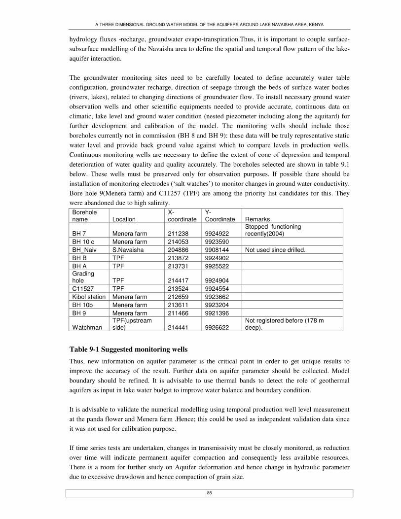
A THREE DIMENSIONAL GROUND WATER MODEL OF THE AQUIFERS AROUND LAKE NAVAISHA AREA, KENYA
85
hydrology fluxes -recharge, groundwater evapo-transpiration.Thus, it is important to couple surface-subsurface modelling of the Navaisha area to define the spatial and temporal flow pattern of the lake-aquifer interaction. The groundwater monitoring sites need to be carefully located to define accurately water table configuration, groundwater recharge, direction of seepage through the beds of surface water bodies (rivers, lakes), related to changing directions of groundwater flow. To install necessary ground water observation wells and other scientific equipments needed to provide accurate, continuous data on climatic, lake level and ground water condition (nested piezometer including along the aquitard) for further development and calibration of the model. The monitoring wells should include those boreholes currently not in commission (BH 8 and BH 9): these data will be truly representative static water level and provide back ground value against which to compare levels in production wells. Continuous monitoring wells are necessary to define the extent of cone of depression and temporal deterioration of water quality and quality accurately. The boreholes selected are shown in table 9.1 below. These wells must be preserved only for observation purposes. If possible there should be installation of monitoring electrodes (‘salt watches’) to monitor changes in ground water conductivity. Bore hole 9(Menera farm) and C11257 (TPF) are among the priority list candidates for this. They were abandoned due to high salinity. Borehole name Location
X-coordinate
Y-Coordinate Remarks
BH 7 Menera farm 211238 9924922 Stopped functioning recently(2004)
BH 10 c Menera farm 214053 9923590 BH_Naiv S.Navaisha 204886 9908144 Not used since drilled. BH B TPF 213872 9924902 BH A TPF 213731 9925522 Grading hole TPF 214417 9924904 C11527 TPF 213524 9924554 Kibol station Menera farm 212659 9923662 BH 10b Menera farm 213611 9923204 BH 9 Menera farm 211466 9921396
Watchman TPF(upstream side) 214441 9926622
Not registered before (178 m deep).
Table 9-1 Suggested monitoring wells Thus, new information on aquifer parameter is the critical point in order to get unique results to improve the accuracy of the result. Further data on aquifer parameter should be collected. Model boundary should be refined. It is advisable to use thermal bands to detect the role of geothermal aquifers as input in lake water budget to improve water balance and boundary condition. It is advisable to validate the numerical modelling using temporal production well level measurement at the panda flower and Menera farm .Hence; this could be used as independent validation data since it was not used for calibration purpose. If time series tests are undertaken, changes in transmissivity must be closely monitored, as reduction over time will indicate permanent aquifer compaction and consequently less available resources. There is a room for further study on Aquifer deformation and hence change in hydraulic parameter due to excessive drawdown and hence compaction of grain size.
A THREE DIMENSIONAL GROUND WATER MODEL OF THE AQUIFERS AROUND LAKE NAVAISHA AREA, KENYA
86
The use of pilot points in conjunction with zonal parameterization could be applied in similar way to the adjacent Elementata-Nakuru area model calibration to get a realistic model There is an opportunity for the application of distributed three-dimensional models, within the framework of GIS (with GMS interface) as an approach which permits data to be continually updated, standardized and integrated. Also this can be supported by visualization tools. The GIS module (in GMS) can be used to display data from a GIS database directly in GMS without having to convert that data to GMS data types. Native GMS data such as grids and boreholes can be displayed along with the GIS data. The GIS module can also be used to select a portion of the GIS data and convert it to GMS data types to be used in constructing a groundwater model. Thus, there is a need to study and formulate a well organized database for the project area. Some data that would contribute a great deal to future studies and modelling of the Navaisha aquifers would be:
• Additional continuously daily ground water level measurements in those boreholes or wells where data is scarce.
• Temporal variability study of recharge and other fluxes.. • At present, additional model calibration is needed in several model reaches for which
suitable data were unavailable.Alternatively,uncertainity in the models can be significantly reduced through collection of additional data to support the calibration effort, including:
• Hydraulic characterization of water table gradients to or from the river, to support refinement of surface water/aquifer interaction. It needs to redevelop the conceptual model of the aquifer. In particular, the role of the rivers, need to be investigated further. It is difficult to guess whether the river is feeding, gaining or both or as an outlet via structurally controlled like Gilgil and Karati river.

A THREE DIMENSIONAL GROUND WATER MODEL OF THE AQUIFERS AROUND LAKE NAVAISHA AREA, KENYA
87
REFERENCES Allison, G. B. (1987). "A review of the Physical Chemical and Isotopic techniques available for
Estimating Groundwater Recharge." In I. Simmers, ed. 222. 49-72. Anderson M. P., a. J. A. M. (1981). "Seasonal reversals of ground water flow around lakes and
relevance to stagnation points and lake budgets." Water Resources Research 17(4): 1139-1150.
Anderson M.P., W. W. W. (1992). Applied Groundwater Modeling - Simulation Flow and Advective Transport, Academic Press, Inc.
Anderson.M.P. a. X. C. (1993). "Long and short term transience in a ground water/lake system in Winsconsin, U.S.A." Journal of Hydrology 145: 1-18.
Appelo, C. A. J., and Postma, D., (1996). Geochemistry, groundwater and pollution: Third corrected print, A.A. Balkema Publishers.Netherlands, ,.
Aqua search (2001). Water Resources Assessment Study, Menera farm, Naivasha, Water resources projectDelamera Estates ltd.
Asfaque (1999). Estimating lake evaporation using metreological data and remote sensing. WREM. Enshede, ITC.
Baher (1997). Surface water -ground water interaction, Lake Navaisha,Kenya. WREM. Enshede, ITC.
Bwire Ojiambo, S., W. Berry Lyons, et al. (2003). "Strontium isotopes and rare earth elements as tracers of groundwater-lake water interactions, Lake Naivasha, Kenya." Applied Geochemistry 18(11): 1789-1805.
Cheng. A. M. P. a. (1993). "Long and short term transience in a ground water /lake system in Wisconsin,USA." Hydrolgy 145: 1-18.
Chilton J (1971). Nairobi Conservation area annual survey Report 1970:various maps.,. Nairobi, Water development Division,Misnstry of Agriculture.
Clarke A.C.G., D. A., G.Darling. (1990). Geological,Volcanolgical and Hydrogeolgical controls on the occurrence of the Geothermal activity in the area surrounding Lake Navaisha,. Kenya, Minstry of Energy, Republic of kenya.
de Marsily, G. (1986). Quantitative Hydrogeology. Academic press: 440. Farah, H. O. (2001). Estimation of Regional Evaporation under different weather condition from
Satellite and Meteorological data : A case study in the Naivasha basin, Kenya., University, Wageningen: 170.
Franke, O. L., T.E.Reilly, and G.d.Bennet, (1987). Definition of boundary and initial conditions in the analysis of saturated ground water flow systems:, USGS.
Githae, I. T. (1998). Ground water flow modelling as a tool for water balance assessments,case study,Nakuru-Elementata basin within the kenyan rift valley system. Ground water Hydrolgy. Delft, IHE.
Goldson John (1993). A three phase environmental impact study of recent developments around lake Navaisha: Phase 1, Associates for the lake Navaisha Riparian owners association.
Graham, A. (1998). Ground water recharge estimation of the Malewa catchment,Navasha -Kenya. WREM. Enschede, ITC.
Hermandez, R. R. (1999). Ground water flow modeling of Navaisha basin, Kenya. WREM. Enshede, ITC.
Hill MC, C. R., Pollock DW (1998). "A controlled experiment in ground water flow model calibration.Ground water."
Hunt.R.J., J. T. k. (1996). "The application of analytic element model to investigate ground water -lake interactions at pretty Lake,Wisconsin." Journal of Lake and Reservoir Management 12(4): 487-495.
Jacob.Baer (1992). Ground water issue, Fundamental of ground water modeling. United state Envirnomental Protection Agency.
John.Doherty (2004). Model independent parameter estimation user manual, Water mark computing,Australia.
Jyrkama., M. I., sykes,J.F.,Normani,S.D., (2002). "Recharge estimation for transient ground water modelling." Ground Water 40(6): 638-648.

A THREE DIMENSIONAL GROUND WATER MODEL OF THE AQUIFERS AROUND LAKE NAVAISHA AREA, KENYA
88
Kibona (2000). Temporal & spatial variation of ground water level north of lake Navaisha, Kenya. WREM. Enshede, ITC.
Krasny, J. (1997). "Transmissivity and permeabilty distribution in hard rock envirnoment.InPointet,T(ed) Hard rock hydrosystem." IAHS 241: 81-90.
Kresic, N. (1997). "Quantitative solutions in hydrogeology and ground water modeling." Lee (1996). "Numerical simulation of lake using high conductivity technique with three
dimensional flow model." USGS. Lee, T. M. (1996). "Hydro-geologic controls on the groundwater interactions with an acidic lake in
karst terrain, Lake Barco, Florida." Water Resources Research 32(no 4): 831-844. Long, J. C. S., Remer,j.s.Wilson,C.R and witherspoon,P.A (1982). "porous media equivalents
networks of discontinous fractures." Water Resources Research 18(3): 645-658. M.K.Arusei, J. K. S. a. M. P. T. (1996). The outflow of lake Naviasha based on the stable isoptope
composition. Mcann, D. L. (1974). Hydrogeolgic investigation of rift valley catchments, United nations-kenyan
government geothermal exploration project. McDonald, M. G., and A.W.Harbaugh (1988). A modular three-dimensional finite-difference ground-
water flow model, U.s.Geological .survey.tech.water resources.Invest.,. McDonald, M. G., Harbaugh,A.W., (1996). A modular three dimensional finite differnce ground
water flow model. washington, USGS. Meijerink, A. M. J., de brouwer,H.A.M.,Mannerts,C.M. and Valenzuela,C.R. (1994). "Introduction to
the use of information systems for practical hydrology." ITC,enschede,The Netherlands. Mekonnen (1999). Determination of regional scale crop coefficents from crop water requirement
calculations.A Remote sensing perspective.A case study of the Lake Navaisha basin. WREM. Enschede, ITC.
Merrit, M. L., and L.F.konikow. (2000). Documentataion of computer program to simulate lake-aquifer interaction using the MODFLOW ground water flow model and the MOC3D solute-transport model, U.s.Geological survey water resources Investig.
Mmbui (1999). A study of the long term water balance of the lake Navaisha,kenya. WREM. Enshede, ITC.
Morgan, D. S. (1988). Geohydrology and numerical model analysis of ground water flow in the Goose Lake Basin,Oregon and California., U.S geological survey Water resources. Investigation.
Muno, F. A. (2002). Water balance of the southern Kenya rift valley lakes. WREM. Enschede, ITC. Nabidi, I. K. (2002). Development of 3-D conceptual hydrogeological model for Lake Navaisha area.
WREM. Enschede, ITC. Nalugya, E. (2003). Estimation of direct recharge of natural vegetations of the lake aquifer : a case study of Lake Naivasha basin,Kenya. WREM. Enschede, ITC. Nassima Atmaoui., Dirk Hollnack(2003)” Neotectonics and extension direction of the Southern Kenya Rift, Lake Magadi area” Tectonophysics Journal 364: 71– 83 Ne-Zheng.Sun (1994). Inverse problems in ground water modelling. haifa,Israel. Ojiambo, B. S. (1992). Hydrogeolgic, Hydrogeochemical and Stable isotopic study of possible
interactions between Lake Navaisha,shallow subsurface and Olkaria Geothermal. Reno, Nevada.
Ojiambo, B. S. (1996). Characterization of subsurface outflow from a closed basin freshwater tropical lake ,Rift valley, Kenya. Reno, Nevada.
Oppong-Boateng, R. (2001). Assessment of the use of Groundwater for Irrigation in the Southern part of Lake Naivasha. Water resources evaluation and management. Enschede, ITC.
Ower (2000). The long term interaction of ground water with lake Navaisha,Kenya. WREM. Enschede, ITC.
Richard C. Aster, B. B., and Clifford Thurber1 (2003). Parameter Estimation and Inverse Problems. Sanchez-Vila., C., J.,Girardi,j.P., (1996). "Scale effects in transmissivity." Journal of Hydrology
183(1-2): 1-22. Scanlon, B. R., P.G. Cook, and R.W. Healy. (2002). "Choosing appropriate Techniques for
quantifying Groundwater Recharge." International Association of Hydro-geologists 10: 18-39.

A THREE DIMENSIONAL GROUND WATER MODEL OF THE AQUIFERS AROUND LAKE NAVAISHA AREA, KENYA
89
Simmers, I., J.J. De Vries, and J. Jacobus. (2002). "An overview of processes and challenges. International Association of Hydro-geologists." IAH International Association 10: 8-16.
Singhal (1997). "Volcanic hydraulic parameters." Singhal, B. B. S. (1997). "Hydro-geological chractertics of Deccan trap formations of India.In
:Pointet,T(ed) Hard rock hydrosystems." IAHS 241: 75-80. Snow, D. T. (1969). "Anisotropic permeability of fractured media." Water Resources Research 5: 86-
95. Spitez, K. a. M., j., (1996). A practical guide to ground water and solute transport modelling, John
Wiley and Sons Inc. Stuttard, M. J., J.hayball, G.Narcos, M.Suppo, R.catani, L.Isavwa, J.baraza and A., Oroda (1995).
Monitoring lakes in Kenya: An environmental Analysis Methodology for developing countries, Final report to European commision, Contract.
Tenalem, A. (1998). The hydrogeolgical system of the Lake District basin, Central main Ethiopian rift. ITC publication, PhD thesis. Enschede, Free university of Amsterdam: 259.
Trottman, D. K. (1997). Modelling ground water storage change in response to fluctuating levels of lake Navaisha, Kenya. WREM. Enschede, ITC.
Tsiboah, T. (2002). 2-D resistivity & time domain EM in aquifer mapping, a case study, north of lake Navaisha,Kenya. EREG. Enschede, ITC.
VIAK (1975). Naivasha water supply project,, Minstry of Agriculture,Rebublic of Kenya. W.Berry Lyons., S. B. O., Welch, Kathy A.,Poreda., Robert J., Karen H.Johannesson (2003).
"Strontium isotopes and rare earth elements as tracers of groundwater-lake water interactions, Lake Naivasha, Kenya." Applied Geochemistry 18(11): 1789-1805.
Wiberg, I. (1976). Navaisha Water supply project,Ground water Investigation,, VIAKEA Ltd.,Consulting Engineering and Mapping Services.
Winter, T. (1976). "Numerical simulation analysis of steady state,three dimensional ground water flow near lakes." Water Resources Research 14: 245-254.
Zhang, L., Dawes, W.r., Hatton, T., Reece (1999). "Estimation of soil moisture and ground water recharge using TOPOG_IRM model." Water Resources Research 35(1): 149-161.
Ziji, W. (1999). "Scale aspects of groundwater flow and transport systems." Hydrogeology Journal 7: 139-150.
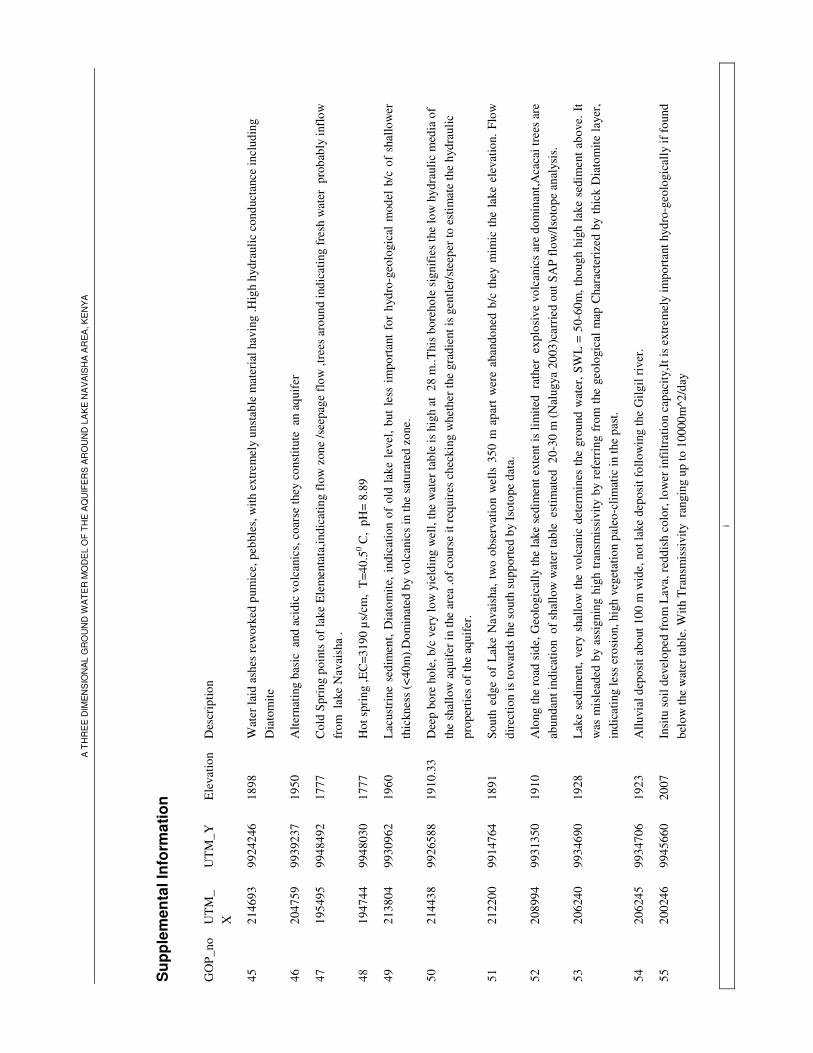
A T
HR
EE
DIM
EN
SIO
NA
L G
RO
UN
D W
AT
ER
MO
DE
L O
F T
HE
AQ
UIF
ER
S A
RO
UN
D L
AK
E N
AV
AIS
HA
AR
EA
, KE
NY
A
i
Sup
plem
enta
l Inf
orm
atio
n
GO
P_no
U
TM
_X
U
TM
_Y
Ele
vatio
n D
escr
iptio
n
45
2146
93
9924
246
1898
W
ater
laid
ash
es re
wor
ked
pum
ice,
peb
bles
, with
ext
rem
ely
unst
able
mat
eria
l hav
ing
.Hig
h hy
drau
lic c
ondu
ctan
ce in
clud
ing
Dia
tom
ite
46
2047
59
9939
237
1950
A
ltern
atin
g ba
sic
and
aci
dic
volc
anic
s, c
oars
e th
ey c
onst
itute
an
aqui
fer
47
1954
95
9948
492
1777
C
old
Spri
ng p
oint
s of
lake
Ele
men
tata
,indi
catin
g flo
w z
one
/see
page
flow
,tre
es a
roun
d in
dica
ting
fres
h w
ater
pro
babl
y in
flow
fr
om l
ake
Nav
aish
a .
48
1947
44
9948
030
1777
H
ot s
prin
g ,E
C=3
190
µs/c
m,
T=4
0.50 C
, pH
= 8.
89
49
2138
04
9930
962
1960
La
cust
rine
sed
imen
t, D
iato
mite
, ind
icat
ion
of o
ld l
ake
leve
l, bu
t le
ss i
mpo
rtan
t fo
r hy
dro-
geol
ogic
al m
odel
b/c
of
shal
low
er
thic
knes
s (<
40m
).Dom
inat
ed b
y vo
lcan
ics
in th
e sa
tura
ted
zone
.
50
2144
38
9926
588
1910
.33
Dee
p bo
re h
ole,
b/c
ver
y lo
w y
ield
ing
wel
l, th
e w
ater
tabl
e is
hig
h at
28
m..T
his
bore
hole
sig
nifie
s th
e lo
w h
ydra
ulic
med
ia o
f th
e sh
allo
w a
quife
r in
the
area
.of c
ours
e it
requ
ires
che
ckin
g w
heth
er th
e gr
adie
nt is
gen
tler/
stee
per t
o es
timat
e th
e hy
drau
lic
prop
ertie
s of
the
aqui
fer.
51
2122
00
9914
764
1891
So
uth
edge
of
Lake
Nav
aish
a, t
wo
obse
rvat
ion
wel
ls 3
50 m
apa
rt w
ere
aban
done
d b/
c th
ey m
imic
the
lak
e el
evat
ion.
Flo
w
dire
ctio
n is
tow
ards
the
sout
h su
ppor
ted
by Is
otop
e da
ta.
52
2089
94
9931
350
1910
A
long
the
road
sid
e, G
eolo
gica
lly th
e la
ke s
edim
ent e
xten
t is
limite
d ra
ther
exp
losi
ve v
olca
nics
are
dom
inan
t,Aca
cai t
rees
are
ab
unda
nt in
dica
tion
of s
hallo
w w
ater
tabl
e e
stim
ated
20-
30 m
(Nal
ugya
200
3)ca
rrie
d ou
t SA
P flo
w/I
soto
pe a
naly
sis.
53
2062
40
9934
690
1928
La
ke s
edim
ent,
very
sha
llow
the
volc
anic
det
erm
ines
the
grou
nd w
ater
, SW
L =
50-6
0m, t
houg
h hi
gh la
ke s
edim
ent a
bove
. It
was
mis
lead
ed b
y as
sign
ing
high
tran
smis
sivi
ty b
y re
ferr
ing
from
the
geol
ogic
al m
ap C
hara
cter
ized
by
thic
k D
iato
mite
laye
r, in
dica
ting
less
ero
sion
, hig
h ve
geta
tion
pale
o-cl
imat
ic in
the
past
.
54
2062
45
9934
706
1923
A
lluvi
al d
epos
it ab
out 1
00 m
wid
e, n
ot la
ke d
epos
it fo
llow
ing
the
Gilg
il ri
ver.
55
2002
46
9945
660
2007
In
situ
soi
l dev
elop
ed fr
om L
ava,
redd
ish
colo
r, lo
wer
infil
trat
ion
capa
city
,It is
ext
rem
ely
impo
rtan
t hyd
ro-g
eolo
gica
lly if
foun
d
belo
w th
e w
ater
tabl
e. W
ith T
rans
mis
sivi
ty r
angi
ng u
p to
100
00m
^2/d
ay

A T
HR
EE
DIM
EN
SIO
NA
L G
RO
UN
D W
AT
ER
MO
DE
L O
F T
HE
AQ
UIF
ER
S A
RO
UN
D L
AK
E N
AV
AIS
HA
AR
EA
, KE
NY
A
ii
56
1999
35
9945
946
1982
E
xcel
lent
out
cro
p of
Tuf
fs &
lapi
lli w
ith
pyro
clas
tic (p
umic
e) a
nd l
ava
flow
/gilg
i Tra
chyt
e la
yer o
ffse
tted
by fa
ult r
unni
ng
60 0 N
W
57
1975
00
9950
616
1902
D
iato
mite
lay
er i
nter
-bed
ded
w
ith c
oars
e &
fin
e
depo
sits
. I
nver
se g
radi
ng
from
fin
e(bo
ttom
)- c
oars
e (t
op)
ind
icat
ing
la
ke s
edim
ent d
epos
it w
ith g
reen
ish
& r
eddi
sh c
olor
..
58
2155
33
9928
546
2041
Sp
ring
59
1987
26
9952
626
2078
M
ajom
onto
hot
spr
ing,
geo
logi
cally
do
min
ated
by
collu
vium
s de
posi
t Fau
lt/co
ntac
t spr
ing?
EC
= 29
8 µs
/cm
, pH
= 7
, Q
=
750l
/s
60
1974
16
9950
714
1876
La
cust
rine
sed
imen
t int
rude
d by
igni
mbr
ite, b
otto
m o
f the
val
ley,
faul
t run
ning
NN
W-S
SE, r
iver
bed
infil
trat
ion
is li
kely
alo
ng
the
faul
t lin
e w
here
the
rive
r has
a s
trai
ght l
ine.
61
1973
15
9950
626
1876
R
iver
flo
w lo
ss o
f 35
% f
rom
ups
trea
m d
ue ir
riga
tion
or in
filtr
atio
n. N
eeds
to e
xpla
in f
or q
ualit
y &
qua
ntity
det
erio
ratio
n by
m
ass
bala
nce
EC
= 59
2 µs
/cm
, pH
=7.
3, Q
= 20
l/s
62
1967
95
9950
062
1871
Q
uarr
y si
te, n
ear
to l
ake
Ele
men
tata
, sho
wn
with
thi
ck D
iato
mite
70
m t
hick
alte
rnat
ing
with
goo
d aq
uife
r (c
oars
e m
ater
ial)
in
clud
ing
the
laye
r as
a co
nfin
ing
bed.
63
1898
03
9959
588
1861
Le
ft s
ide
of th
e B
aro
rive
r w
ith h
igh
infil
trat
ion
capa
city
, no
dra
inag
e(sa
ndy)
64
1884
66
9960
622
1873
M
eror
ine
rive
r, fa
ult c
ontr
olle
d ri
ver
incl
udin
g th
e ot
her G
ilgil
trib
utar
y pr
obab
ly w
ith h
igh
infil
trat
ion
65
1907
05
9956
426
1799
B
aruk
rive
r, Q
= 10
0l/s
, TD
S= 8
0mg/
l, E
C=
168
µs/c
m
66
1898
26
9956
788
1816
Pr
oduc
tive
Bor
ehol
e w
ith n
o pi
pe l
ine,
war
m s
team
com
ing
out
of t
he B
H. E
C=4
09 µ
s/cm
, T=
300 C
pH
=7.0
4, T
DS=
200
m
g/l,
Isot
ope
sam
ple
was
take
n.
67
1900
90
9956
928
1790
R
iver
Con
fluen
ce ri
ver t
erra
ces
depo
sit.
EC
= 29
5 µs
/cm
pH
= 7,
Q=1
l/s.
68
1896
61
9956
724
1808
A
lluvi
al fi
ll , M
erer
uni r
iver
69
1994
38
9900
322
1920
R
ecen
t vo
lcan
ic ,
<200
yea
rs, n
o ve
geta
tion/
soil
deve
lope
d w
hich
is s
imila
r to
wes
t of E
lem
enta
ta b
asin
70
1854
20
9950
439
1779
W
est o
f Lak
e E
lem
enat
a s
alin
e w
ith b
are
vege
tatio
n
71
1956
17
9947
569
1779
So
uth
rim
of
la
ke
Ele
men
tata
.Hig
hly
crac
ked
clay
ey
soil.
In
dica
ting
sign
ifica
nce
wat
er
hold
ing
capa
city
fo
r ev
apor
atio
n/re
char
ge -
swel
ling
-cra
ckin
g re
spon
se. T
his
shou
ld b
e co
nsid
ered
in th
e w
ater
bal
ance
com
puta
tion.
Unl
ike
lake
N
avai
sha
beca
use
it ha
s le
ss fl
uctu
atio
n an
d no
cla
yey
soil.
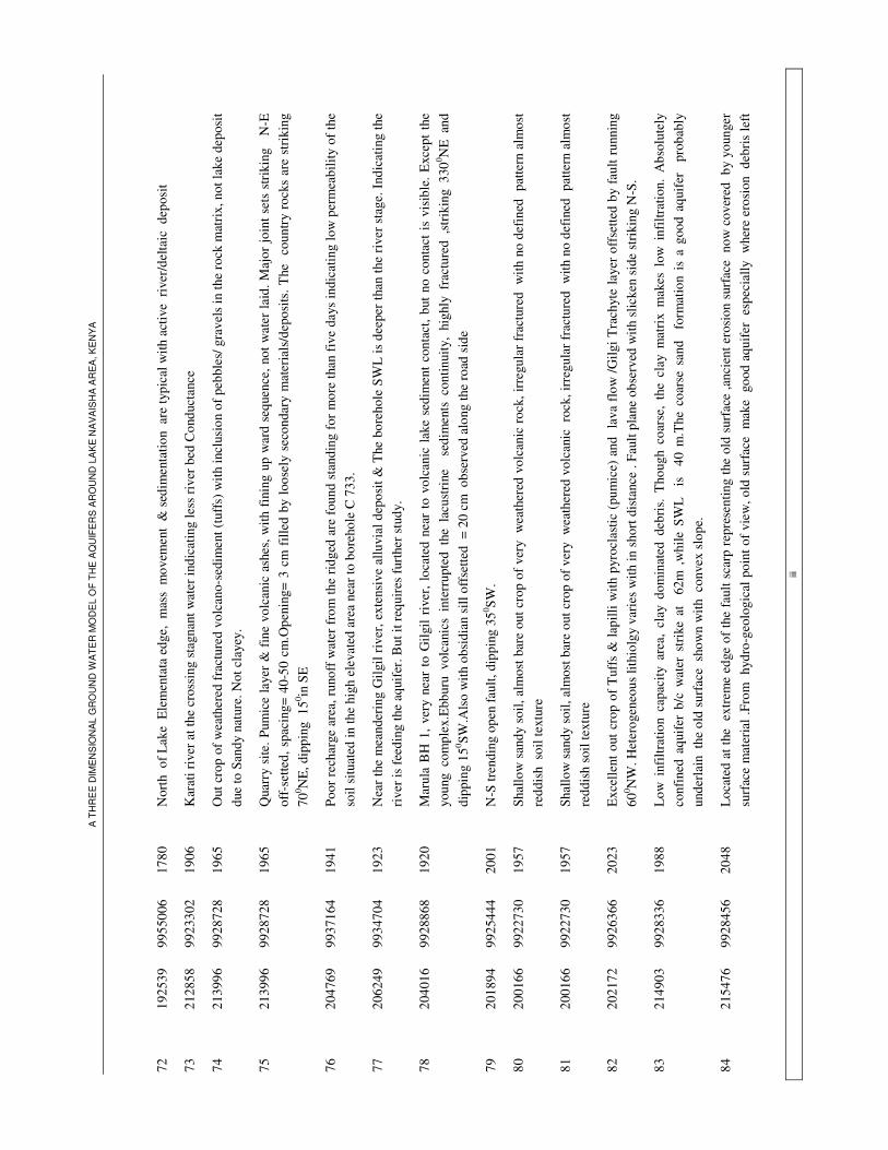
A T
HR
EE
DIM
EN
SIO
NA
L G
RO
UN
D W
AT
ER
MO
DE
L O
F T
HE
AQ
UIF
ER
S A
RO
UN
D L
AK
E N
AV
AIS
HA
AR
EA
, KE
NY
A
iii
72
1925
39
9955
006
1780
N
orth
of L
ake
Ele
men
tata
edg
e, m
ass
mov
emen
t &
sed
imen
tatio
n a
re ty
pica
l with
act
ive
rive
r/de
ltaic
dep
osit
73
2128
58
9923
302
1906
K
arat
i riv
er a
t the
cro
ssin
g st
agna
nt w
ater
indi
catin
g le
ss ri
ver b
ed C
ondu
ctan
ce
74
2139
96
9928
728
1965
O
ut c
rop
of w
eath
ered
frac
ture
d vo
lcan
o-se
dim
ent (
tuff
s) w
ith in
clus
ion
of p
ebbl
es/ g
rave
ls in
the
rock
mat
rix,
not
lake
dep
osit
due
to S
andy
nat
ure.
Not
cla
yey.
75
2139
96
9928
728
1965
Q
uarr
y si
te. P
umic
e la
yer
& f
ine
volc
anic
ash
es, w
ith f
inin
g up
war
d se
quen
ce, n
ot w
ater
laid
. Maj
or jo
int s
ets
stri
king
N
-E
off-
sette
d, s
paci
ng=
40-5
0 cm
.Ope
ning
= 3
cm f
illed
by
loos
ely
seco
ndar
y m
ater
ials
/dep
osits
. The
co
untr
y ro
cks
are
stri
king
70
0 NE
, dip
ping
150 in
SE
76
2047
69
9937
164
1941
Po
or r
echa
rge
area
, run
off w
ater
from
the
ridg
ed a
re fo
und
stan
ding
for
mor
e th
an fi
ve d
ays
indi
catin
g lo
w p
erm
eabi
lity
of th
e so
il si
tuat
ed in
the
high
ele
vate
d ar
ea n
ear t
o bo
reho
le C
733
.
77
2062
49
9934
704
1923
N
ear
the
mea
nder
ing
Gilg
il ri
ver,
exte
nsiv
e al
luvi
al d
epos
it &
The
bor
ehol
e SW
L is
dee
per
than
the
rive
r sta
ge. I
ndic
atin
g th
e ri
ver i
s fe
edin
g th
e aq
uife
r. B
ut it
requ
ires
furt
her s
tudy
.
78
2040
16
9928
868
1920
M
arul
a B
H 1
, ve
ry n
ear
to G
ilgil
rive
r, lo
cate
d ne
ar t
o vo
lcan
ic l
ake
sedi
men
t co
ntac
t, bu
t no
con
tact
is
visi
ble.
Exc
ept
the
youn
g co
mpl
ex.E
bbur
u vo
lcan
ics
inte
rrup
ted
the
lacu
stri
ne
sedi
men
ts c
ontin
uity
, hi
ghly
fra
ctur
ed ,
stri
king
330
0 NE
and
di
ppin
g 15
0 SW.A
lso
with
obs
idia
n si
ll of
fset
ted
= 2
0 cm
obs
erve
d al
ong
the
road
sid
e
79
2018
94
9925
444
2001
N
-S tr
endi
ng o
pen
faul
t, di
ppin
g 35
0 SW.
80
2001
66
9922
730
1957
Sh
allo
w s
andy
soi
l, al
mos
t bar
e ou
t cro
p of
ver
y w
eath
ered
vol
cani
c ro
ck, i
rreg
ular
frac
ture
d w
ith n
o de
fined
pat
tern
alm
ost
redd
ish
soi
l tex
ture
81
2001
66
9922
730
1957
Sh
allo
w s
andy
soi
l, al
mos
t bar
e ou
t cro
p of
ver
y w
eath
ered
vol
cani
c ro
ck, i
rreg
ular
frac
ture
d w
ith n
o de
fined
pat
tern
alm
ost
redd
ish
soil
text
ure
82
2021
72
9926
366
2023
E
xcel
lent
out
cro
p of
Tuf
fs &
lapi
lli w
ith p
yroc
last
ic (
pum
ice)
and
lav
a flo
w /G
ilgi T
rach
yte
laye
r of
fset
ted
by f
ault
runn
ing
600 N
W. H
eter
ogen
eous
lith
iolg
y va
ries
with
in s
hort
dis
tanc
e . F
ault
plan
e ob
serv
ed w
ith s
licke
n si
de s
trik
ing
N-S
.
83
2149
03
9928
336
1988
Lo
w i
nfilt
ratio
n ca
paci
ty a
rea,
cla
y do
min
ated
deb
ris.
Tho
ugh
coar
se,
the
clay
mat
rix
mak
es l
ow i
nfilt
ratio
n. A
bsol
utel
y co
nfin
ed a
quife
r b/
c w
ater
str
ike
at
62m
,w
hile
SW
L i
s 4
0 m
.The
coa
rse
sand
fo
rmat
ion
is a
goo
d aq
uife
r p
roba
bly
un
derl
ain
the
old
surf
ace
sho
wn
with
con
vex
slop
e.
84
2154
76
9928
456
2048
Lo
cate
d at
the
ext
rem
e ed
ge o
f th
e fa
ult s
carp
rep
rese
ntin
g th
e ol
d su
rfac
e ,a
ncie
nt e
rosi
on s
urfa
ce n
ow c
over
ed b
y yo
unge
r su
rfac
e m
ater
ial .
From
hyd
ro-g
eolo
gica
l poi
nt o
f vie
w, o
ld s
urfa
ce m
ake
goo
d aq
uife
r e
spec
ially
whe
re e
rosi
on d
ebri
s le
ft

A T
HR
EE
DIM
EN
SIO
NA
L G
RO
UN
D W
AT
ER
MO
DE
L O
F T
HE
AQ
UIF
ER
S A
RO
UN
D L
AK
E N
AV
AIS
HA
AR
EA
, KE
NY
A
iv
behi
nd i
s co
arse
r in
natu
re
85
2143
07
9925
104
1914
T
rach
yte
ridg
e, h
ighl
y jo
inte
d, d
ippi
ng S
SW 1
00.T
he T
rach
yte
stri
kes
alm
ost N
-S.c
onsi
dere
d as
no
flow
bou
ndar
y. N
eeds
to
chec
k w
heth
er th
ere
is a
con
tinui
ty o
f the
lake
sed
imen
ts o
n ei
ther
sid
e.
86
1975
81
9919
294
1897
N
o sp
ring
s at
the
faul
t sca
rp(2
50m
) run
ning
N-S
indi
catin
g pe
rvio
us n
atur
e of
the
faul
t pla
ne. V
ery
larg
e tr
ees
at th
e fo
ot o
f the
sc
arp
with
int
ense
veg
etat
ion.
Sha
llow
er w
ater
tab
le a
t th
e do
wnt
hrow
n si
de,
a bo
reho
le w
ith S
WL
=11m
.The
Bor
ehol
e is
pu
mpi
ng u
p th
e up
thro
w s
ide
by s
tret
ched
pip
e lin
e.
87
1974
00
9919
997
1996
O
pen
faul
t, yo
ung
runn
ing
850 N
with
ope
ning
> 2
.5m
cro
ssin
g th
e fa
ult s
carp
at h
igh
angl
e. P
ossi
ble
pref
eren
tial c
hann
el f
or
the
out f
low
88
2032
34
9928
318
1981
M
esay
e G
orge
, les
s jo
inte
d yo
ung
volc
anic
, int
rudi
ng th
e la
ke s
edim
ent.
The
lake
sed
imen
t is
foun
d un
derl
ying
the
volc
anic
fe
w jo
int s
ets
runn
ing
800 E
,and
join
t bed
str
ikin
g 3
20 N, a
bout
10c
m o
peni
ng. w
ith m
icro
fol
d .it
s ax
is o
rien
ting
at
400 N
89
2075
40
9930
925
1907
Lo
w in
filtr
atio
n ca
paci
ty, L
acus
trin
e de
posi
t, ne
ar b
eaut
y lin
e. R
ain
Wat
er s
tand
ing
for l
ong
time.
90
2134
38
9924
992
1915
N
o D
iato
mite
laye
r in
this
are
a ex
cept
in G
ilgil
,Mal
wa
,Osl
aria
but
may
mis
lead
if i
t has
thin
lay
er. T
he c
lay
laye
r in
dica
tes
it is
like
ly
lake
sed
imen
t .T
his
sedi
men
t (20
-30
m)i
s d
ue to
the
dow
n th
row
sid
e o
f th
e ar
ea w
here
a f
ault
is e
xpec
ted
but
ne
eds
to b
e ve
rifie
d fr
om g
eolo
gica
l map
.
91
2144
17
9924
904
1923
A
t th
e fo
ot o
f T
rach
yte
ridg
e, c
an b
e co
nsid
ered
as
no f
low
bou
ndar
y. P
umic
e la
yer
is l
ikel
y fo
und
at s
hallo
wer
dep
th a
t su
bsur
face
.
92
2144
98
9924
986
1984
A
t the
top
of th
e T
rach
yte
ridg
e lo
cate
d in
pan
da fl
ower
far
m, s
teep
ly d
ippi
ng T
rach
yte,
str
ikin
g 24
00 N, d
ippi
ng 1
450 S
alm
ost
perp
endi
cula
r to
the
stri
ke. F
avor
s to
rec
harg
e p
anda
flow
er a
rea
to a
littl
e bi
t .it
is s
light
ly jo
inte
d .It
has
dis
tinct
veg
etat
ion
whi
ch ty
pica
lly g
row
s in
trac
hyte
terr
ain
in th
e s
urro
undi
ngs
of th
e ar
ea
93
2145
80
9927
144
1953
N
ear w
atch
man
cam
p, D
istin
ct la
nd s
cape
and
veg
etat
ion.
Tra
chyt
e
94
2143
91
9928
362
1978
Fu
lly c
ollu
vium
s, re
wor
ked
volc
anic
dep
osit
(pum
ice)
. Lon
g tr
ench
qua
rry
site
100
m lo
ng 2
m w
ide
and
2 m
dee
p
95
2140
32
9928
648
1965
E
xcel
lent
out
crop
, qua
rry
site
, com
pose
d v
arie
ty o
f vo
lcan
ic ro
cks/
pyro
clas
ts, s
teep
ly d
ippi
ng p
umic
e
96
2130
55
9927
970
1933
N
ice
out
crop
Out
crop
of
fluvi
al w
ith t
hin
gran
ular
mat
eria
l in
ter-
bedd
ed w
ith i
n th
e lo
osel
y cl
ayey
san
d so
il. T
rach
yte,
Pu
mic
e, w
elde
d T
rach
yte.
Dom
inat
ed b
y sa
ndy
text
ure.
Dia
tom
ite la
yer.
97
2198
75
9928
140
1924
R
oad
geol
ogy,
vol
cani
c as
h m
ost
likel
y fa
llen
on t
he l
ake
botto
m .W
ell
stra
tifie
d, p
erfe
ctly
hor
izon
tal.
The
col
laps
ible
san
d la
yer w
as c
lear
ly s
how
n

A T
HR
EE
DIM
EN
SIO
NA
L G
RO
UN
D W
AT
ER
MO
DE
L O
F T
HE
AQ
UIF
ER
S A
RO
UN
D L
AK
E N
AV
AIS
HA
AR
EA
, KE
NY
A
v
98
2133
79
9924
382
1913
Ju
st a
t the
ben
d of
kar
ati r
iver
, whe
re f
ault
lines
int
erse
ct.C
harc
teri
zed
by d
ense
veg
eata
ion.
Nee
ds to
und
erst
and
from
whe
re
the
plan
ts t
rans
pire
b/c
the
SW
L is
>30
m, i
.e 2
4 m
bel
ow t
he r
iver
bed
. The
cap
illar
y zo
ne /f
ring
e m
ight
be
high
. The
riv
er
cond
ucta
nce
is li
kely
to b
e lo
w d
ue
tp p
rese
nce
of s
tagn
ant w
ater
alo
ng th
e ri
ver b
ed
99
2091
85
9927
033
1907
A
long
the
road
sid
e ne
ar to
Mar
ula
farm
sho
wn
with
thic
k (>
4m) c
laye
y so
il, fi
ne &
loos
e te
xtur
e, fo
und
exte
nsiv
ely.
100
2151
63
9919
650
1950
Fo
ot o
f th
e fa
ult
scar
p, e
ast
of l
ake
Nav
aish
a ou
t cr
op o
f la
ke d
epos
it (p
umic
e),
no j
oint
. W
ell
sort
ed c
oars
e la
yer
is
inte
rcal
ated
with
fine
r lay
er h
avin
g di
stin
ct c
olor
. sho
wn
alte
rnat
ing
fine
with
coa
rse
laye
r
101
2131
09
9917
934
1888
U
ntra
ced
piez
omet
ric
flow
lin
e w
heth
er i
t is
away
fro
m/to
war
ds th
e la
ke o
r el
se i
nter
cept
ed b
y fa
ults
run
ning
nor
th-s
outh
. It
need
s ac
cura
te le
velin
g of
wel
ls to
def
ine
flow
dir
ectio
n (r
efer
to B
ehar
(M
Sc, 1
999)
cro
ss s
ectio
n). W
ater
flo
ws
tow
ards
the
lake
from
the
ridg
e bu
t aga
in w
ater
flow
s aw
ay fr
om th
e la
ke to
war
ds th
e ri
dge
.puz
zlin
g w
here
the
wat
er g
oes?
102
2150
26
9917
410
1910
La
ke o
ut f
low
sou
th w
ard
supp
orte
d by
iso
tope
dat
a. H
ydra
ulic
gra
dien
t is
low
(ne
eds
geod
etic
lev
elin
g).
man
y o
f th
e bo
reho
les
mim
ic th
e la
ke le
vel
103
2135
88
9914
292
1925
K
arag
ita
villa
ge n
o bo
reho
le a
roun
d, e
nvir
onm
enta
lly h
as s
eptic
tank
pro
blem
.
104
2120
65
9914
820
1923
C
alde
ra ri
m la
ke ,
Cre
scen
t la
nd ,
very
dee
p (1
7m),
no s
edim
enta
tion
105
2133
4 99
1355
6 18
93
Exc
elle
nt p
umic
e ou
t cro
p ,h
ighl
y pe
rmea
ble
& tr
ansm
issv
ity v
alue
if fo
und
in th
e sa
tura
ted
zone
106
2133
80
9912
224
1892
So
uthe
rn o
f th
e la
ke m
ore
of s
alin
e un
like
the
nort
hern
par
t of t
he la
ke .
unfo
rtun
ate
to ir
riga
te th
e ar
ea w
here
the
out f
low
is
expe
cted
107
1985
21
9905
444
1935
C
ontin
uous
sha
llow
aqu
ifer
term
inat
es d
ue a
bsen
ce o
f co
nfin
ing
laye
r .p
roba
bly
feed
ing
the
deep
aqu
ifer.
Shal
low
wat
er ta
ble
is m
issi
ng. G
roun
d w
ater
esc
apes
out
as
a st
eam
from
the
cavi
ties
show
n.
108
1943
73
9911
952
1942
V
olca
nic
ash
depo
sit w
ith to
p la
yer
diat
omite
ind
icat
ing
lake
dep
osit
109
1894
82
9914
058
1925
N
adib
ibi
plai
n ri
ver
is s
eepi
ng i
n to
kar
astic
cle
arly
sho
wn
in t
he i
mag
e .N
ot c
lear
ly k
now
n w
here
it
goes
. It
nee
ds d
etai
l fr
actu
re s
tudy
.
110
1947
90
9913
750
1952
C
rate
r lak
e, c
onsi
dere
d as
hug
e du
g w
ell f
ully
repr
esen
ting
the
grou
nd w
ater
. It i
s gr
ound
wat
er la
ke. F
ully
de
pend
ent.1
00%
is fr
om g
roun
d w
ater
b/c
ET
>>ra
infa
ll. W
ater
is fl
owin
g to
war
ds th
e cr
ater
lake
from
Nav
aish
a la
ke.N
avai
sha
lake
is a
bit
high
er e
leva
tion
than
cra
ter l
ake.
Dom
inat
ed b
y vo
lcan
ic (p
yroc
last
ic)-
surg
e de
posi
ts. I
t ha
s is
otop
ic s
igna
ture
with
18O
=12.
43,
2 D =
59.
3.
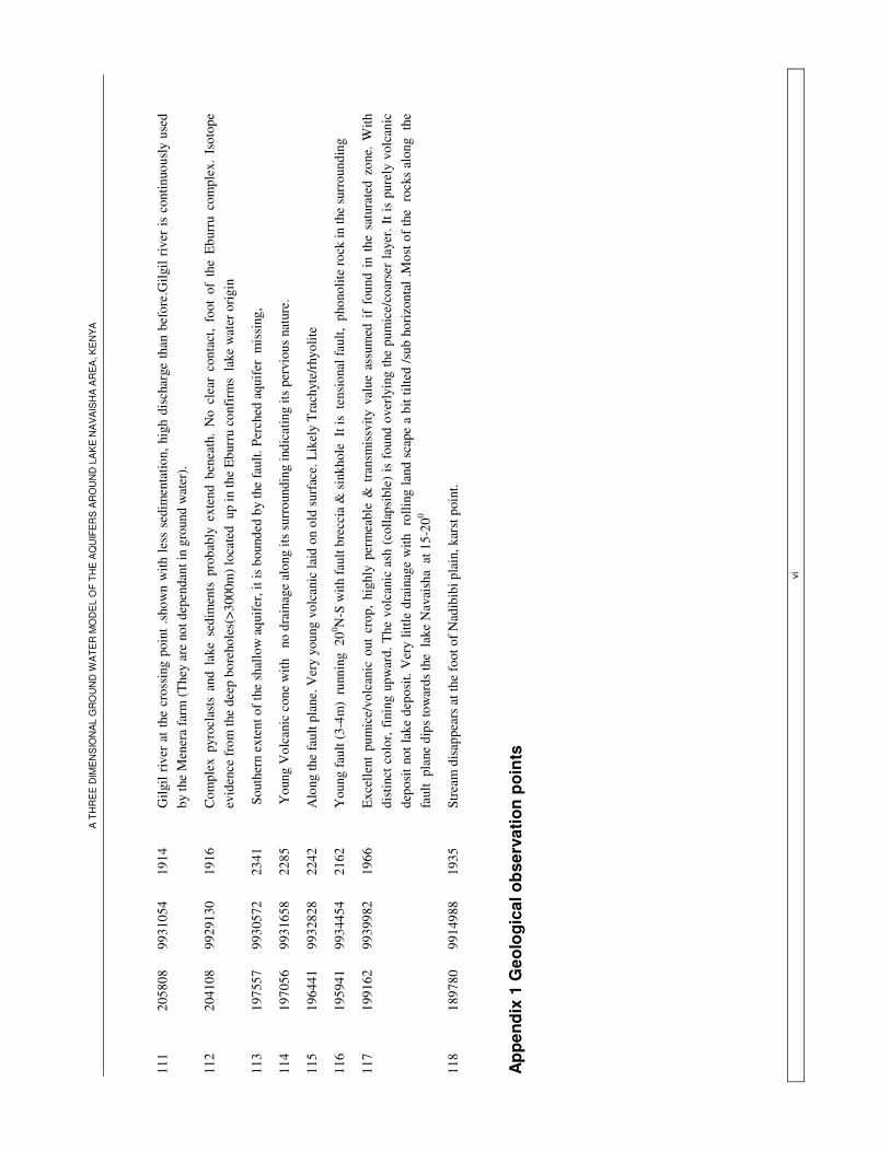
A T
HR
EE
DIM
EN
SIO
NA
L G
RO
UN
D W
AT
ER
MO
DE
L O
F T
HE
AQ
UIF
ER
S A
RO
UN
D L
AK
E N
AV
AIS
HA
AR
EA
, KE
NY
A
vi
111
2058
08
9931
054
1914
G
ilgil
rive
r at
the
cros
sing
poi
nt .s
how
n w
ith le
ss s
edim
enta
tion,
hig
h di
scha
rge
than
bef
ore.
Gilg
il ri
ver
is c
ontin
uous
ly u
sed
by th
e M
ener
a fa
rm (T
hey
are
not d
epen
dant
in g
roun
d w
ater
).
112
2041
08
9929
130
1916
C
ompl
ex p
yroc
last
s an
d la
ke s
edim
ents
pro
babl
y ex
tend
ben
eath
. N
o cl
ear
cont
act,
foot
of
the
Ebu
rru
com
plex
. Is
otop
e ev
iden
ce fr
om th
e de
ep b
oreh
oles
(>30
00m
) loc
ated
up
in th
e E
burr
u co
nfir
ms
lake
wat
er o
rigi
n
113
1975
57
9930
572
2341
S
outh
ern
exte
nt o
f the
sha
llow
aqu
ifer,
it is
bou
nded
by
the
faul
t. Pe
rche
d aq
uife
r m
issi
ng,
114
1970
56
9931
658
2285
Y
oung
Vol
cani
c co
ne w
ith
no d
rain
age
alon
g its
sur
roun
ding
indi
catin
g its
per
viou
s na
ture
.
115
1964
41
9932
828
2242
A
long
the
faul
t pla
ne. V
ery
youn
g vo
lcan
ic la
id o
n ol
d su
rfac
e. L
ikel
y T
rach
yte/
rhyo
lite
116
1959
41
9934
454
2162
Y
oung
faul
t (3-
4m)
runn
ing
200 N
-S w
ith fa
ult b
recc
ia &
sin
khol
e It
is t
ensi
onal
faul
t, p
hono
lite
rock
in th
e su
rrou
ndin
g
117
1991
62
9939
982
1966
E
xcel
lent
pum
ice/
volc
anic
out
cro
p, h
ighl
y pe
rmea
ble
& t
rans
mis
svity
val
ue a
ssum
ed i
f fo
und
in t
he s
atur
ated
zon
e. W
ith
dist
inct
col
or, f
inin
g up
war
d. T
he v
olca
nic
ash
(col
laps
ible
) is
fou
nd o
verl
ying
the
pum
ice/
coar
ser
laye
r. It
is p
urel
y vo
lcan
ic
depo
sit n
ot la
ke d
epos
it. V
ery
little
dra
inag
e w
ith r
ollin
g la
nd s
cape
a b
it til
ted
/sub
hor
izon
tal .
Mos
t of
the
roc
ks a
long
the
fa
ult
plan
e di
ps to
war
ds th
e la
ke N
avai
sha
at 1
5-20
0
118
1897
80
9914
988
1935
St
ream
dis
appe
ars
at th
e fo
ot o
f Nad
ibib
i pla
in, k
arst
poi
nt.
App
endi
x 1
Geo
logi
cal o
bser
vatio
n po
ints

A THREE DIMENSIONAL GROUND WATER MODEL OF THE AQUIFERS AROUND LAKE NAVAISHA AREA, KENYA
vii
Owner/ Location UTM_X UTM_Y Source Altitude Measured by/Year Three Point Ostrich 213518 9924527 Differential GPS 1999 1910.00 Isah 2001 Three Point Ostrich 213735 9925528 Differential GPS 1999 1915.00 Kibona 1999 Three Point Ostrich 213713 9924977 Differential GPS 1999 1911.00 Kibona 1999 Three Point Ostrich 213459 9924929 Differential GPS 1999 1909.00 Kibona 1999 Three Point Ostrich 214004 9925600 Differential GPS 1999 1918.00 Kibona 1999 Three Point Ostrich 213544 9925720 Differential GPS 1999 1917.00 Kibona 1999 Manera Farm 211437 9921386 Differential GPS 1999 1891.00 Opiyo (averaged)1999 Milk factory 211914 9924455 Differential GPS 1999 1904.00 Opiyo (averaged)1999 DTI Insitute (BH103) 213101 9928951 Differential GPS 1999 1940.00 Nairobi Data base 1960 BH107 214504 9926572 Differential GPS 1999 1940.01 Opiyo 1975 Kobil station 212603 9923764 Differential GPS 1999 1902.00 Kibona 1999 Marula Farm (Irish artist) 210473 9928944 Differential GPS 1999 1894.00 Kibona 1999 C11954 203360 9925256 Geodetic leveled (1999) 1938.30 Opiyo (averaged)1999 BH2 Manera Farm 211323 9922533 Geodetic leveled (2001) 1892.58 Ochieng/Sipul and Isah BH7 Manera Farm 211231 9924924 Geodetic leveled (2001) 1903.32 Ochieng/Sipul and Isah BOINEETBH1 (Brig Farm) 194375 9919316 Geodetic leveled (2001) 1927.12 Ochieng/Sipul and Isah BOINEETBH2 (Brig Farm) 194608 9918650 Geodetic leveled (2001) 1922.20 Ochieng/Sipul and Isah GOLFCOURSEBH2 (up) 201561 9926470 Geodetic leveled (2001) 2075.75 Ochieng/Sipul and Isah ISRAELBH1/Beauty Line 208323 9931189 Geodetic leveled (2001) 1899.15 Ochieng/Sipul and Isah KEDONGBH 214204 9907097 Geodetic leveled (2001) 2022.93 Ochieng/Sipul and Isah KONGONIAICBH 194827 9909902 Geodetic leveled (2001) 1902.99 Ochieng/Sipul and Isah
New sher well 207857 9908376
Surveyed with respect to sher peg level(sipul)=1905.88 1905.74 Ochieng/Sipul and Isah
Kedong C210 208867 9909074
Surveyed with respect to sher peg level(sipul)=1905.88 1899.13 Ochieng/Sipul and Isah
Hearther 214281 9909564 Levelled with refernce to previously levelled 1975.50 Ochieng/Sipul and Isah
TPO(BH-D) 213397 9924862 1908.874 Yohannes 2004
TPO(BH-G) 213362 9924894 1908.909 Yohannes 2004
TPO(BH-F) 213397 9924804 1908.83 Yohannes 2004
TPO(BH-Watchman) 214441 9926622 1910.33 Yohannes 2004
TPO(BH-Grading) 214417 9924904 1915.53 Yohannes 2004
Yohannes 2004
Appendix 2. Levelled wells in the study area

A THREE DIMENSIONAL GROUND WATER MODEL OF THE AQUIFERS AROUND LAKE NAVAISHA AREA, KENYA
viii
Appendix 3. Interpretation of well C11527 Geological Log Clearly Indicates existence of two aquifers
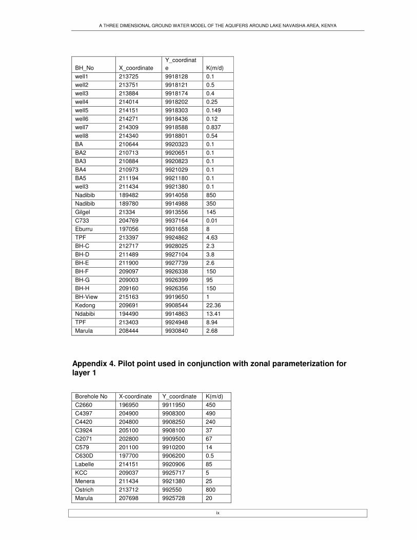
A THREE DIMENSIONAL GROUND WATER MODEL OF THE AQUIFERS AROUND LAKE NAVAISHA AREA, KENYA
ix
BH_No X_coordinate Y_coordinate K(m/d)
well1 213725 9918128 0.1 well2 213751 9918121 0.5 well3 213884 9918174 0.4 well4 214014 9918202 0.25 well5 214151 9918303 0.149 well6 214271 9918436 0.12 well7 214309 9918588 0.837 well8 214340 9918801 0.54 BA 210644 9920323 0.1 BA2 210713 9920651 0.1 BA3 210884 9920823 0.1 BA4 210973 9921029 0.1 BA5 211194 9921180 0.1 well3 211434 9921380 0.1 Nadibib 189482 9914058 850 Nadibib 189780 9914988 350 Gilgel 21334 9913556 145 C733 204769 9937164 0.01 Eburru 197056 9931658 8 TPF 213397 9924862 4.63 BH-C 212717 9928025 2.3 BH-D 211489 9927104 3.8 BH-E 211900 9927739 2.6 BH-F 209097 9926338 150 BH-G 209003 9926399 95 BH-H 209160 9926356 150 BH-View 215163 9919650 1 Kedong 209691 9908544 22.36 Ndabibi 194490 9914863 13.41 TPF 213403 9924948 8.94 Marula 208444 9930840 2.68
Appendix 4. Pilot point used in conjunction with zonal parameterization for layer 1
Borehole No X-coordinate Y_coordinate K(m/d) C2660 196950 9911950 450 C4397 204900 9908300 490 C4420 204800 9908250 240 C3924 205100 9908100 37 C2071 202800 9909500 67 C579 201100 9910200 14 C630D 197700 9906200 0.5 Labelle 214151 9920906 85 KCC 209037 9925717 5 Menera 211434 9921380 25 Ostrich 213712 992550 800 Marula 207698 9925728 20
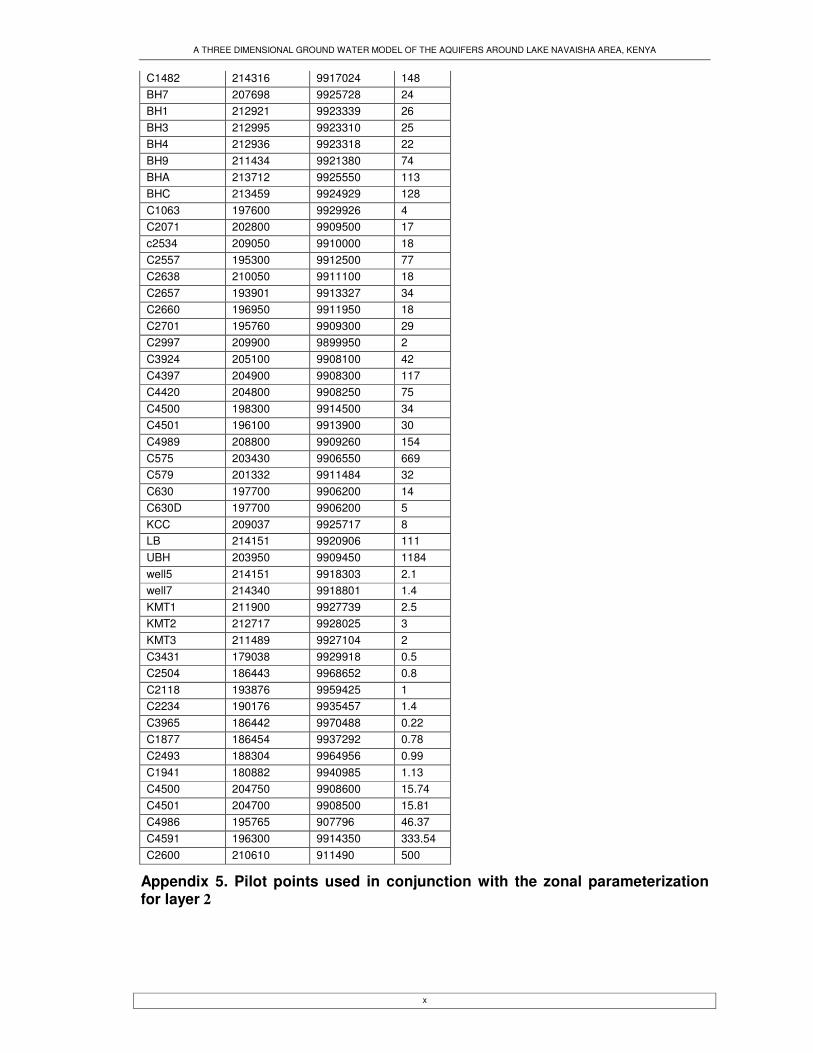
A THREE DIMENSIONAL GROUND WATER MODEL OF THE AQUIFERS AROUND LAKE NAVAISHA AREA, KENYA
x
C1482 214316 9917024 148 BH7 207698 9925728 24 BH1 212921 9923339 26 BH3 212995 9923310 25 BH4 212936 9923318 22 BH9 211434 9921380 74 BHA 213712 9925550 113 BHC 213459 9924929 128 C1063 197600 9929926 4 C2071 202800 9909500 17 c2534 209050 9910000 18 C2557 195300 9912500 77 C2638 210050 9911100 18 C2657 193901 9913327 34 C2660 196950 9911950 18 C2701 195760 9909300 29 C2997 209900 9899950 2 C3924 205100 9908100 42 C4397 204900 9908300 117 C4420 204800 9908250 75 C4500 198300 9914500 34 C4501 196100 9913900 30 C4989 208800 9909260 154 C575 203430 9906550 669 C579 201332 9911484 32 C630 197700 9906200 14 C630D 197700 9906200 5 KCC 209037 9925717 8 LB 214151 9920906 111 UBH 203950 9909450 1184 well5 214151 9918303 2.1 well7 214340 9918801 1.4 KMT1 211900 9927739 2.5 KMT2 212717 9928025 3 KMT3 211489 9927104 2 C3431 179038 9929918 0.5 C2504 186443 9968652 0.8 C2118 193876 9959425 1 C2234 190176 9935457 1.4 C3965 186442 9970488 0.22 C1877 186454 9937292 0.78 C2493 188304 9964956 0.99 C1941 180882 9940985 1.13 C4500 204750 9908600 15.74 C4501 204700 9908500 15.81 C4986 195765 907796 46.37 C4591 196300 9914350 333.54 C2600 210610 911490 500
Appendix 5. Pilot points used in conjunction with the zonal parameterization for layer 2

A THREE DIMENSIONAL GROUND WATER MODEL OF THE AQUIFERS AROUND LAKE NAVAISHA AREA, KENYA
xi
Appendix 6 Groundwater flow map for the natural setting prior to 1980(By ower 2000)
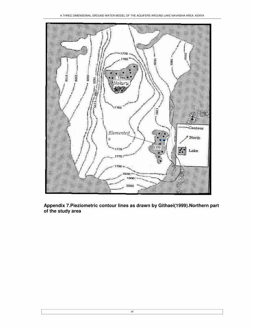
A THREE DIMENSIONAL GROUND WATER MODEL OF THE AQUIFERS AROUND LAKE NAVAISHA AREA, KENYA
xii
Appendix 7.Pieziometric contour lines as drawn by Githaei(1999).Northern part of the study area

A THREE DIMENSIONAL GROUND WATER MODEL OF THE AQUIFERS AROUND LAKE NAVAISHA AREA, KENYA
xiii
)()()(
)( BhLl
AhBhatCh +×−=
Appendix 8.Calculating the General Head Boundary
(0,hA)
(l,hB)w
l
L
C
B
A

A THREE DIMENSIONAL GROUND WATER MODEL OF THE AQUIFERS AROUND LAKE NAVAISHA AREA, KENYA
xiv
Appendix: 9 Current Piezometric Head Contours. W indicates the depression due to extraction from the well field.
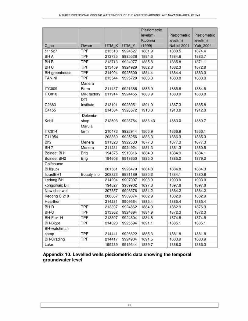
A THREE DIMENSIONAL GROUND WATER MODEL OF THE AQUIFERS AROUND LAKE NAVAISHA AREA, KENYA
xv
C_no Owner UTM_X UTM_Y
Pieziometric level(m) Kibonna (1999)
Pieziometric level(m) Nabidi 2001
Pieziometric level(m) Yoh_2004
c11527 TPF 213518 9924527 1881.9 1880.5 1874.4 BH A TPF 213735 9925528 1884.6 1884.6 1883.7 BH B TPF 213713 9924977 1885.8 1885.8 1871.1 BH C TPF 213459 9924929 1882.3 1882.3 1872.8 BH-greenhouse TPF 214004 9925600 1884.4 1884.4 1883.0 TANINI TPF 213544 9925720 1883.8 1883.8 1883.0
ITC009 Manera Farm 211437 9921386 1885.9 1885.6 1884.5
ITC010 Milk factory 211914 9924455 1883.9 1883.9 1883.0
C2883 DTI Institute 213101 9928951 1891.0 1887.3 1885.8
C4155 214504 9926572 1913.0 1913.0 1912.0
Kobil Delemia-shop 212603 9923764 1883.43 1883.0 1880.7
ITC014 Marula farm 210473 9928944 1866.9 1866.9 1866.1
C11954 203360 9925256 1886.3 1886.3 1885.3 Bh2 Menera 211323 9922533 1877.3 1877.3 1877.3 BH 7 Menera 211231 9924924 1881.3 1881.3 1880.5 Boineet BH1 Brig 194375 9919316 1884.9 1884.9 1884.1 Boineet BH2 Brig 194608 9918650 1885.0 1885.0 1879.2 Golfcourse BH2(up) 201561 9926470 1884.8 1884.8 1884.3 IsraelBH1 Beauty line 208323 9931189 1885.2 1884.1 1880.8 kedong BH 214204 9907097 1903.9 1903.9 1903.9 kongoniaic BH 194827 9909902 1897.8 1897.8 1897.8 New sher well 207857 9908376 1884.2 1884.2 1884.2 Kedong C 210 208867 9909074 1882.9 1882.9 1882.9 Hearther 214281 9909564 1885.4 1885.4 1885.4 BH-D TPF 213397 9924862 1884.9 1882.9 1876.9 BH-G TPF 213362 9924894 1884.9 1872.3 1872.3 BH-F or H TPF 213397 9924804 1884.8 1874.8 1874.8 BH-Bigot TPF 214023 9925594 1891.1 1885.1 1885.1 BH-watchman camp TPF 214441 9926622 1885.3 1881.8 1881.8 BH-Grading TPF 214417 9924904 1891.5 1883.9 1883.9 Lake 199289 9919344 1889.7 1888.0 1886.0
Appendix 10. Levelled wells pieziometric data showing the temporal groundwater level