A Replication Study of ‘Why Do Cities Hoard Cash?’ (The Accounting Review, 2009)
ABSTRACT
Gore’s article explores the determinants and implications of cash reserves. We first attempted to
replicate Gore’s finding of a positive relationship between environmental uncertainty and
municipal fund balances (2009) using the same data, the same specifications, and the same
econometric software. We then tested the robustness of her original findings by adding years
and observations. We show that the empirical results reported in this article are largely
replicable and that its results are robust to substantial data extensions. Nevertheless, we believe
that Gore reaches normative conclusions, that municipalities hold “excess cash reserves,” which
are not justified by her empirical results.
Keywords: Reserves • Volatility • Replication
JEL Classification Numbers: H71 • H72
1
A Replication Study of ‘Why Do Cities Hoard Cash?’ (The Accounting Review, 2009)
1. INTRODUCTION
The Government Finance Officer’s Association recommends that municipalities maintain
reserves at least equal to about 16 percent of revenues, plus more to deal with revenue
volatility, infrastructure upkeep and vulnerability to extreme events. Kriz (2002) and Dothan
and Thompson (2009) argue that they should (as a normative matter) increase reserves (fund
balances) in line with revenue volatility. Indeed, Kriz concluded that if the representative
Minnesota municipality wished “to sustain a three percent expenditure growth rate with a 75
percent confidence level, it would need savings equal to 91 percent of total revenues” (Kriz
2002: 5).
Angela Gore’s 2009 article in Accounting Review is especially important because it shows
that local-government fund balances do apparently vary directly with revenue volatility and
that jurisdictions that spend more on administration tend to maintain higher reserves. These
finding are critical to the developing field of public financial management. Consequently, we
wished to pursue them further, especially since we had reservations about Gore’s data set,
specification of response and predictor variables, and functional forms tested. Unfortunately,
her data set and codes were unavailable. Consequently, we set out to replicate her work, as a
first step as precisely as possible, using the same data, the same specifications, and the same
statistical software1 (Stata). Next, we extended the time horizon of her analysis to include all of
the years of data available.
1Gore used SAS to organize (collate and clean) her data and Stata to analyze it.
2
We also briefly address her article’s fundamental hypothesis: that municipalities over
save, i.e., hold more cash than is needed to “provide a constant level of services to citizens,
regardless of revenue volatility” (Gore 2009, 183).
2. REPLICATION OF SAMPLE SELECTION AND DATA CLEANING
Starting from the government finance database2 (Pierson et al. 2014), which has data from the
Census’s annual survey of state and local governments for years between 1967 and 2011, we
restricted our sample to governments with data from years between 1997 and 2003.
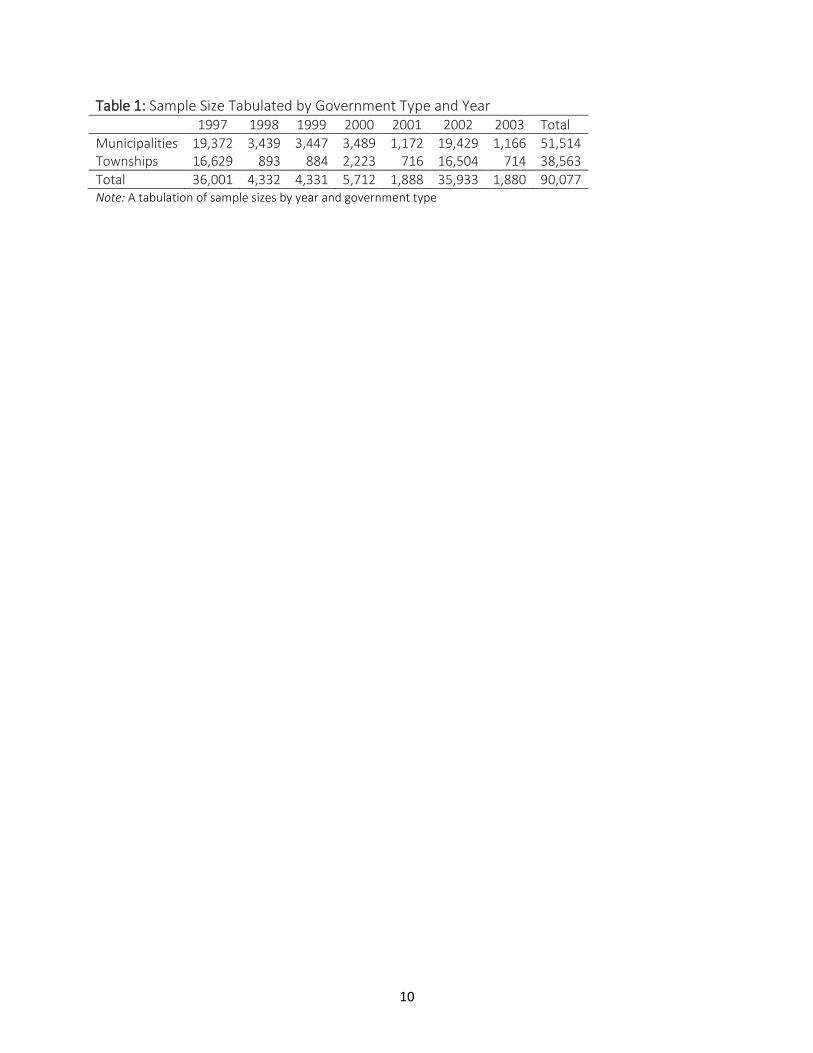
Gore does not explicitly identify the government type codes that she includes in her data
set, but it appears that her analysis comprehends both municipalities (type 2) and townships
(type 3). Table 1 shows the breakdown of the data by year and type of government. It is clear
from this table that using only one government type is too restrictive.
Table 1: Goes about here
Including both municipalities and townships allows us to come close to Gore’s count of
80,125 observations. Unfortunately there is no reasonable way to replicate this number
precisely. Gore may have been working from Census data that had yet to be finalized since the
more recent data from the census includes additional data points.
Gore next drops “4,043 observations with missing data for cash or operating expenses, and
57 observations with apparent errors such as negative debt.” We adopt Gore’s definition of cash
and securities and drop 6,547 observations that have missing values for this variable. We also
drop 505 observations with missing data for total operating expenditure.
It is unclear how Gore calculates total debt from the census data, especially considering
the fact that none of the top-level debt outstanding line items in our data have negative entries.
2 http://www.willamette.edu/mba/research_impact/public_datasets/
3
Given this lack of direction we chose the highest-level variable, total debt outstanding, since it
most closely matches Gore’s language. This leaves us with 83,025 observations, very close to
Gore’s 76,025.
The final data cleaning procedure is described by Gore as: “A total of 66,612 observations
without four years' consecutive data, the minimum number of observations necessary to
estimate the regression models, are also deleted.” When we tried to apply this exactly by
requiring four consecutive years of data we ended up with only 3,003 city-years eligible for our
sample, far less than Gore’s 9,413. This led us down several paths before we realized that she
describes this step on her table 2 in much less restrictive terms as “Less observations for
municipalities with less than four years of data.” When we required our data to have four
previous observations but did not require the years to be consecutive3 we ended up with 9,681
in-sample city-years, within a few hundred of Gore.
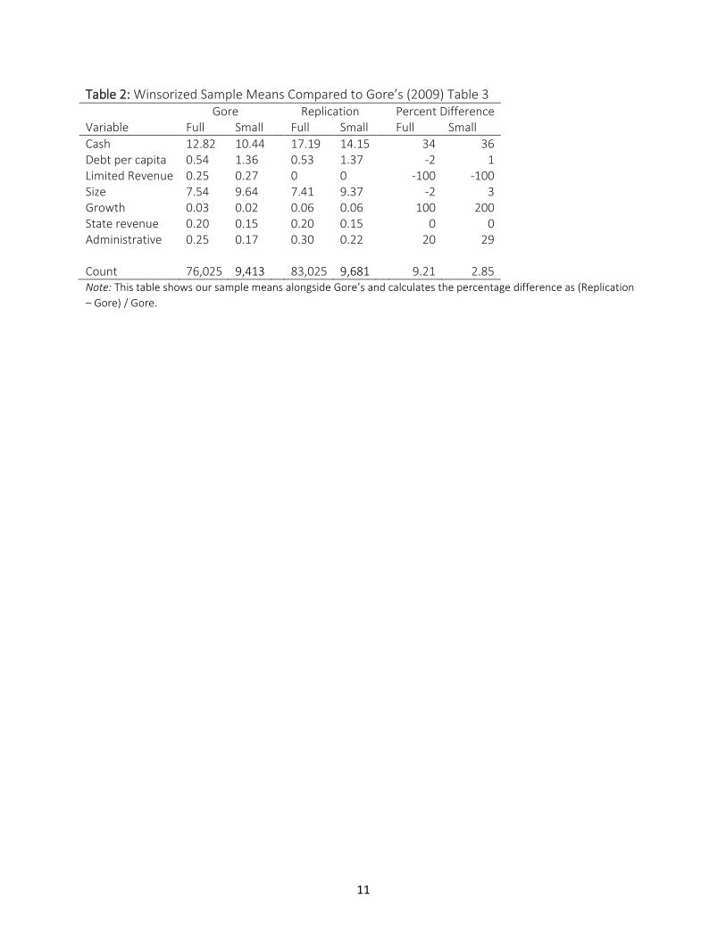
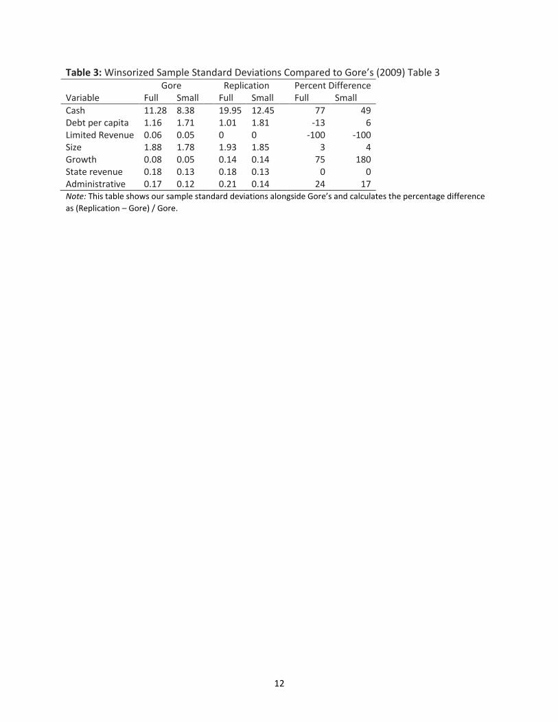
Her table 3 listing sample summary statistics reports winsorized4 summary statistics. She
states that she “winsorizes all of the continuous variables to remove the top and bottom 1
percent” in her section describing her regression results. When we perform a winsorization at
the one percent level separately on both the full sample and the smaller sample we get the
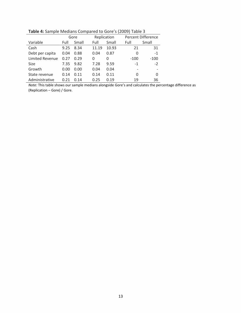
results, shown in tables 2 and 3, which are very close to her results. Sample medians are
reported in table 4 and are also close to those reported by Gore.
3 This causes a few problems when we replicate Gore’s growth variable, since not every city-year in the sample has
a population figure from exactly five years prior, which is what Gore says she uses. Our solution is to use the five-
year population change if it is available, but to substitute a four-year change or a three-year change in the worst
case.
4 A process of setting outlier values to the value of some percentile of the data, “clipping” them but leaving them in
the sample.
4
Table 2: Goes about here
Table 3: Goes about here
Table 4: Goes about here
One particularly troublesome variable, even after winsorizing the sample, is the revenue
diversification index Gore calls “limited revenue.” This variable is described by Gore as “the
product of the fraction of total revenue from each source [property taxes, general sales taxes,
and individual income taxes].” This is almost certainly not correct, either mathematically or
conceptually, since only 212 city-years in our sample have revenue from all three sources, and
therefore almost every value for this variable is equal to zero. There is no way to reconcile this
result with the summary statistics Gore provides or the descriptions of limited revenue in her
paper. We chose to use her construction of limited revenue even though it is not possible to
replicate any of her results for that variable.
2.1. Replication of Results
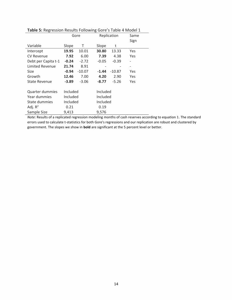
Table 5 displays our results from a regression that is identical to Gore’s table 4 model 1.
Specifically we estimated:5
𝐶𝑎𝑠ℎ/𝐸𝑥𝑝𝑒𝑛𝑑𝑖𝑡𝑢𝑟𝑒𝑠𝑖𝑡
= 𝛼0 + 𝛼1𝐶𝑉𝑟𝑒𝑣𝑒𝑛𝑢𝑒𝑖𝑡 + 𝛼2𝐷𝑒𝑏𝑡 𝑝𝑒𝑟 𝑐𝑎𝑝𝑖𝑡𝑎𝑖𝑡−1
+ 𝛼3𝐿𝑖𝑚𝑖𝑡𝑒𝑑 𝑟𝑒𝑣𝑒𝑛𝑢𝑒𝑖𝑡 + 𝛼4𝑆𝑖𝑧𝑒𝑖𝑡 + 𝛼5𝐺𝑟𝑜𝑤𝑡ℎ𝑖𝑡
+ 𝛼6𝑆𝑡𝑎𝑡𝑒 𝑟𝑒𝑣𝑒𝑛𝑢𝑒𝑖𝑡 + Σ𝛼𝑘𝑄𝑢𝑎𝑟𝑡𝑒𝑟𝑘 + Σ𝛼𝑚𝑆𝑡𝑎𝑡𝑒𝑚
+ Σ𝛼𝑡𝑌𝑒𝑎𝑟𝑡
(1)
5 This model matches Gore’s model from page 188 of her paper, but in her table 4 the subscript of the debt
variable indicates that it is not lagged one year. When we estimated the regression using unlagged debt per capita
the slope estimate changed signs but was still not significant. None of our other slope estimates changed in sign or
significance during that test.
5
The CVrevenue variable is Gore’s measure of revenue volatility. Her paper describes it as: “the
ratio of the standard deviation of total revenue/mean total revenue, over the prior four years
ending at year t [for each local government].” Since our replication found that Gore did not
require four sequential years of data we measured the mean and standard deviation of total
revenue using every year of data available for each city.
Table 5: Goes about here
Our regression results are qualitatively the same as Gore’s for five of the seven estimates
we make. Our estimate of the impact of lagged debt per capita has the same sign as Gore’s
estimate but our estimate is not statistically significant. The biggest difference between the two
sets of results is that in our replication the limited revenue variable was perfectly collinear with
a combination of the other regression variables and needed to be omitted. This reinforces our
finding that Gore’s description of her limited revenue variable was not rich enough to allow
others to replicate her results. Aside from this, our replication of Gore’s model for the months of
cash holdings by local governments confirms her findings for the period between 1997 and
2003. Indeed, our coefficient for the revenue volatility measure is practically identical to hers.
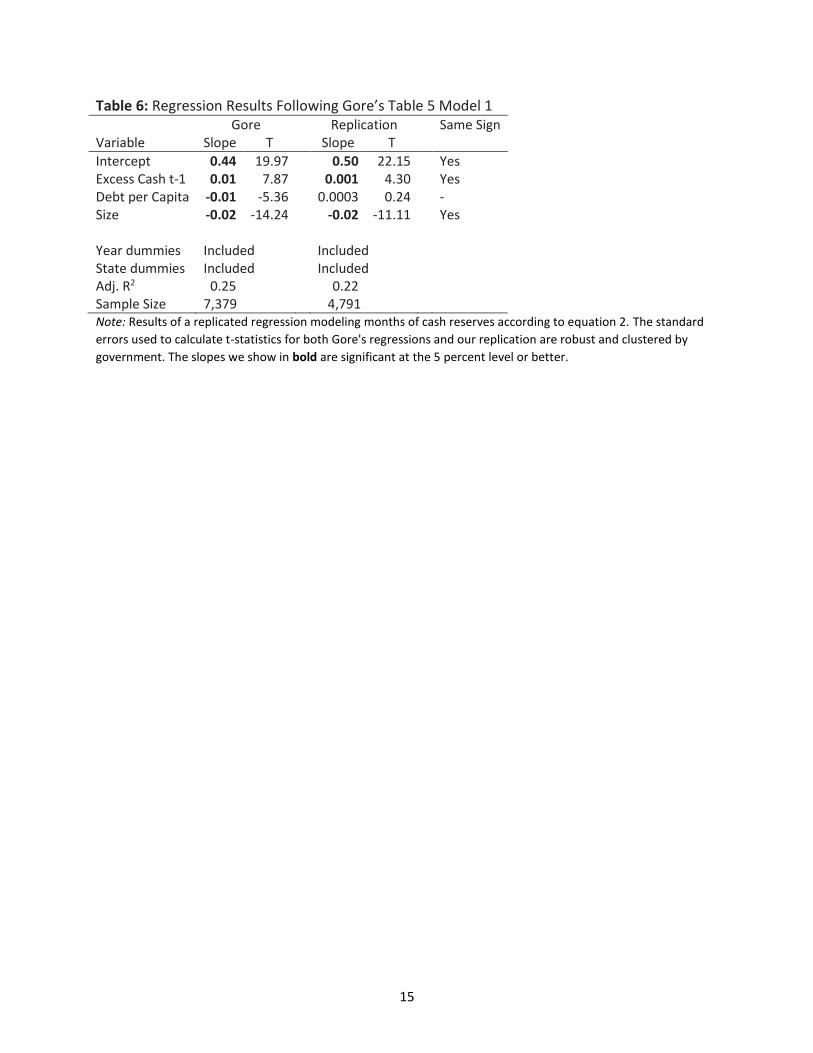
Next we replicated Gore’s table 5 model 1, where she uses the residuals from the first
regression (actual reserves less predicted reserves) to estimate the ratio of administrative
expenses to total operating expenses. Specifically we estimated:
𝐴𝑑𝑚𝑖𝑛𝑖𝑠𝑡𝑟𝑎𝑡𝑖𝑣𝑒𝑖𝑡
= 𝛼0 + 𝛼1𝐸𝑥𝑐𝑒𝑠𝑠 𝑐𝑎𝑠ℎ𝑖𝑡−1 + 𝛼2𝐷𝑒𝑏𝑡 𝑝𝑒𝑟 𝑐𝑎𝑝𝑖𝑡𝑎𝑖𝑡
+ 𝛼3𝑆𝑖𝑧𝑒𝑖𝑡 + Σ𝛼𝑘𝑆𝑡𝑎𝑡𝑒𝑘 + Σ𝛼𝑡𝑌𝑒𝑎𝑟𝑡
(2)
where excess cash is a one year lag of the residuals from the earlier regression.
6
Table 6 shows our results from replicating this regression. Even though our lagged
residuals eliminate far more data than Gore’s do,6 we again qualitatively replicate her results for
every variable except per capita debt.
Table 6: Goes about here
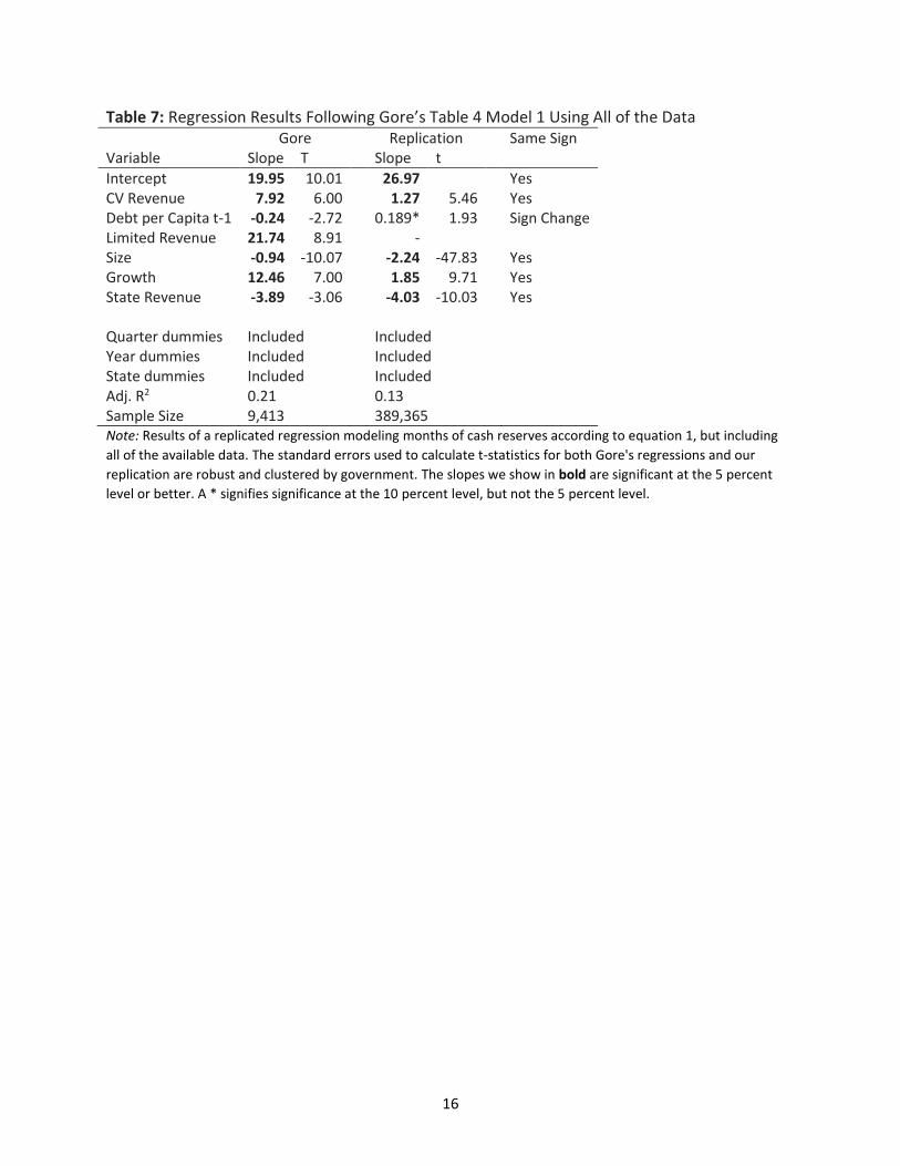
2.2. Sample Extension by Including More Years of Data
Gore’s sample only includes census data between 1997 and 2003, but because the government
finance database has observations between 1967 and 2011 it is reasonable to test whether Gore’s
findings hold when the same statistical tools are applied using more years of data.
In total we were able to include 389,365 city-years of data after applying the same data
cleaning steps that Gore used. Table 7 displays our results.
Table 7: Goes about here
These results are very similar to Gore’s, and to our first replication. The sign of the slope we
estimate for debt per capita is now positive, and is marginally significant (p-value = 0.053), but
Gore’s paper is not focused on the impact that per capita debt has on cash holdings and so we
feel that this difference isn’t important for our replication.
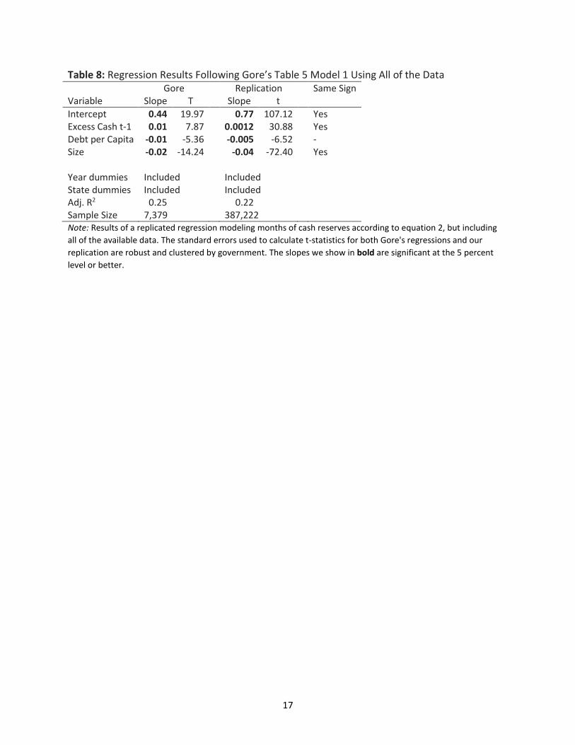
We also replicated the model of administrative expenses as a fraction of total expenses
using the lagged residuals from the first regression. The results of that replication are shown in
table 8, and once again confirm Gore’s findings.
Table 8: Goes about here
3. DISCUSSION AND CONCLUSIONS
6 We found it very difficult to only eliminate 2,000 city-years when lagging the regression residuals, and Gore does
not give any details of how her data managed this.
7
Frankly, in many cases, we would not have handled the data, specified response and predictor
variables, or tested functional forms the way Gore has.7 Nevertheless, the empirical results she
reports in her 2009 article are largely replicable and its main results are robust to substantial
data extensions.8 There is a strong relationship between fiscal uncertainty and reserves.
Municipalities with greater revenue volatility and growth and undiversified revenue sources
tend to hold larger reserves, and larger jurisdictions and those receiving relatively more state
revenue tend to hold less. There is also a statistically significant relationship between
administrative expenses and reserves, i.e., high residuals are correlated with high
administrative expenses and executive salaries; low residuals with low administrative expenses
and executive salaries.
We believe that both of these findings are highly noteworthy. Because her hypothesis, that
municipalities over save, is the mirror image of the conventional view found in the literature,
which argues that governments are, if anything, excessively improvident, findings supporting
the over saving hypothesis (and consequent search for an agency-theoretic explanation) would
be especially meaningful, if valid.
7 As an anonymous reviewer for this journal observed: “It should be pointed out that the two-part procedure of
first estimating cash reserves as a function of policy variables, and then taking the residuals and estimating them
on ‘shirking’ variables is inefficient. All of the variables should be included in a single stage regression and
simultaneously estimated.”
8 And, while this point is beyond the scope of a replication study, we can attest to the robustness of her main result
with respect to data (jurisdictional type), variable specifications (diversity, mean growth and variance, jurisdictional
size, etc.), and econometric software. Indeed, in a majority of cases, we obtained arguably stronger results. As we
worked through the process of replication it seemed, at times, as if she were trying to get results that contradicted
her expectations.
8
However, we believe that Gore fails to sustain this hypothesis. Instead, her argument
involves a rather circular logic. The positive residuals from her first model, which shows a
relationship between environmental uncertainty and fiscal reserves, do not necessarily indicate
excess cash; that these residuals are correlated with administrative costs and salaries could just
as easily have a benign interpretation as a harmful one. For example, Meier and O’Toole (2002,
see also O’Toole and Meier 2011) offer the contrary hypothesis, that administrative expenses or
managerial compensation are reasonable proxies for managerial competence and that more
competent managers would save more for a rainy day. In other words, they argue that the
causation runs from administrative expenses to “extra cash”, rather than the other way around.
It is axiomatic that a finding does not strengthen a hypothesis if the finding in question is
equally consistent with a contrary hypothesis.
To distinguish between these hypotheses, a normative standard or optimum against
which cash holding could be assessed is needed. Gore does not provide one; others do (Kriz
2002; Dothan and Thompson 2009; see also Rameriz 2011). If Kriz is correct, the average
municipality is seriously under saving (i.e., is improvident). If Dothan and Thompson are
correct the average municipality is saving approximately the right amount, but about a third
less than would be optimal. In both cases, therefore, the Meier and O’Toole hypothesis looks
better than Gore’s.
Ultimately, however, we cannot say whether municipalities tend to hold excess reserves,
too little, or just the right amount, and neither, we suspect, can anyone else at this time.
Nevertheless, before we did this analysis, we believed that the likelihood a municipality would
under save was much larger than the likelihood it would over save. Replicating Gore’s work
has caused us to revise our a priori probabilities downward considerably. That remains an
important contribution on her part.
9
REFERENCES
Dothan, Michael U., and Fred Thompson. 2009. A Better Budget Rule. Journal of Policy Analysis
and Management 28 (3): 463-478.
Gore, Angela K. 2009. Why Do Cities Hoard Cash? Determinants and Implications of Municipal
Cash Holdings. The Accounting Review 84 (1): 183-207.
Kriz, Kenneth A. 2002. The Optimal Level of Local Government Fund Balances: A Simulation
Approach. Proceedings of the 95th Annual Conference on Taxation, National Tax Association,
1-7.
Meier, Kenneth J., and Laurence J. O’Toole, Jr. 2002. Public Management and Organizational
Performance: The Effect of Managerial Quality. Journal of Policy Analysis and Management 21
(4): 629-643.
O’Toole, Laurence J., Jr., and Kenneth J. Meier. 2011. Public Management: Organizations,
Governance, and Performance. New York: Cambridge University Press.
Pierson, Kawika, Mike Hand, and Fred Thompson. 2014. The Government Finance Database: A
Common Resource for Quantitative Research in Public Financial Analysis. Center for
Governance and Public Policy Research, Atkinson Graduate School of Management, Willamette
University, Salem, Oregon 97301.
Ramirez, Andres (2011) Nonprofit Cash Holdings: Determinants and Implications. Public
Finance Review 39 (5): 653-681.
Rogers, William H. 1993. Regression Standard Errors in Clustered Samples. Stata Technical
Bulletin Reprints 3 (5): 83-94.
10
Table 1: Sample Size Tabulated by Government Type and Year 1997 1998 1999 2000 2001 2002 2003 Total
Municipalities 19,372 3,439 3,447 3,489 1,172 19,429 1,166 51,514 Townships 16,629 893 884 2,223 716 16,504 714 38,563
Total 36,001 4,332 4,331 5,712 1,888 35,933 1,880 90,077 Note: A tabulation of sample sizes by year and government type
11
Table 2: Winsorized Sample Means Compared to Gore’s (2009) Table 3 Gore Replication Percent Difference Variable Full Small Full Small Full Small
Cash 12.82 10.44 17.19 14.15 34 36 Debt per capita 0.54 1.36 0.53 1.37 -2 1 Limited Revenue 0.25 0.27 0 0 -100 -100 Size 7.54 9.64 7.41 9.37 -2 3 Growth 0.03 0.02 0.06 0.06 100 200 State revenue 0.20 0.15 0.20 0.15 0 0 Administrative 0.25 0.17 0.30 0.22 20 29 Count 76,025 9,413 83,025 9,681 9.21 2.85 Note: This table shows our sample means alongside Gore’s and calculates the percentage difference as (Replication
– Gore) / Gore.
12
Table 3: Winsorized Sample Standard Deviations Compared to Gore’s (2009) Table 3 Gore Replication Percent Difference Variable Full Small Full Small Full Small
Cash 11.28 8.38 19.95 12.45 77 49 Debt per capita 1.16 1.71 1.01 1.81 -13 6 Limited Revenue 0.06 0.05 0 0 -100 -100 Size 1.88 1.78 1.93 1.85 3 4 Growth 0.08 0.05 0.14 0.14 75 180 State revenue 0.18 0.13 0.18 0.13 0 0 Administrative 0.17 0.12 0.21 0.14 24 17 Note: This table shows our sample standard deviations alongside Gore’s and calculates the percentage difference
as (Replication – Gore) / Gore.
13
Table 4: Sample Medians Compared to Gore’s (2009) Table 3 Gore Replication Percent Difference Variable Full Small Full Small Full Small
Cash 9.25 8.34 11.19 10.93 21 31 Debt per capita 0.04 0.88 0.04 0.87 0 -1 Limited Revenue 0.27 0.29 0 0 -100 -100 Size 7.35 9.82 7.28 9.59 -1 -2 Growth 0.00 0.00 0.04 0.04 - - State revenue 0.14 0.11 0.14 0.11 0 0 Administrative 0.21 0.14 0.25 0.19 19 36 Note: This table shows our sample medians alongside Gore’s and calculates the percentage difference as
(Replication – Gore) / Gore.
14
Table 5: Regression Results Following Gore’s Table 4 Model 1 Gore Replication Same
Sign Variable Slope T Slope t
Intercept 19.95 10.01 30.80 13.33 Yes CV Revenue 7.92 6.00 7.39 4.38 Yes Debt per Capita t-1 -0.24 -2.72 -0.05 -0.39 - Limited Revenue 21.74 8.91 - - - Size -0.94 -10.07 -1.44 -10.87 Yes Growth 12.46 7.00 4.20 2.90 Yes State Revenue -3.89 -3.06 -8.77 -5.26 Yes Quarter dummies Included Included Year dummies Included Included State dummies Included Included Adj. R2 0.21 0.19 Sample Size 9,413 9,576 Note: Results of a replicated regression modeling months of cash reserves according to equation 1. The standard
errors used to calculate t-statistics for both Gore's regressions and our replication are robust and clustered by
government. The slopes we show in bold are significant at the 5 percent level or better.
15
Table 6: Regression Results Following Gore’s Table 5 Model 1 Gore Replication Same Sign Variable Slope T Slope T
Intercept 0.44 19.97 0.50 22.15 Yes Excess Cash t-1 0.01 7.87 0.001 4.30 Yes Debt per Capita -0.01 -5.36 0.0003 0.24 - Size -0.02 -14.24 -0.02 -11.11 Yes Year dummies Included Included State dummies Included Included Adj. R2 0.25 0.22 Sample Size 7,379 4,791 Note: Results of a replicated regression modeling months of cash reserves according to equation 2. The standard
errors used to calculate t-statistics for both Gore's regressions and our replication are robust and clustered by
government. The slopes we show in bold are significant at the 5 percent level or better.
16
Table 7: Regression Results Following Gore’s Table 4 Model 1 Using All of the Data Gore Replication Same Sign Variable Slope T Slope t
Intercept 19.95 10.01 26.97 Yes CV Revenue 7.92 6.00 1.27 5.46 Yes Debt per Capita t-1 -0.24 -2.72 0.189* 1.93 Sign Change Limited Revenue 21.74 8.91 - Size -0.94 -10.07 -2.24 -47.83 Yes Growth 12.46 7.00 1.85 9.71 Yes State Revenue -3.89 -3.06 -4.03 -10.03 Yes Quarter dummies Included Included Year dummies Included Included State dummies Included Included Adj. R2 0.21 0.13 Sample Size 9,413 389,365 Note: Results of a replicated regression modeling months of cash reserves according to equation 1, but including
all of the available data. The standard errors used to calculate t-statistics for both Gore's regressions and our
replication are robust and clustered by government. The slopes we show in bold are significant at the 5 percent
level or better. A * signifies significance at the 10 percent level, but not the 5 percent level.
17
Table 8: Regression Results Following Gore’s Table 5 Model 1 Using All of the Data Gore Replication Same Sign Variable Slope T Slope t
Intercept 0.44 19.97 0.77 107.12 Yes Excess Cash t-1 0.01 7.87 0.0012 30.88 Yes Debt per Capita -0.01 -5.36 -0.005 -6.52 - Size -0.02 -14.24 -0.04 -72.40 Yes Year dummies Included Included State dummies Included Included Adj. R2 0.25 0.22 Sample Size 7,379 387,222 Note: Results of a replicated regression modeling months of cash reserves according to equation 2, but including
all of the available data. The standard errors used to calculate t-statistics for both Gore's regressions and our
replication are robust and clustered by government. The slopes we show in bold are significant at the 5 percent
level or better.