Natarajan Meghanathan et al. (Eds) : NeTCoM, CSIT, GRAPH-HOC, SPTM - 2014
pp. 165–183, 2014. © CS & IT-CSCP 2014 DOI : 10.5121/csit.2014.41314
A NEW SURVEY ON BICLUSTERING OF
MICROARRAY DATA
Haifa Ben Saber
1,2 and Mourad Elloumi
1,3
1Laboratory of Technologies of Information and Communication and Electrical
Engineering (LaTICE) at National Superior School of Engineers of Tunis
(ENSIT) - Tunis university, Tunis, Tunisia 2Time université
3University of Tunis-El Manar, Tunisia
[email protected],[email protected]
ABSTRACT
There are subsets of genes that have similar behavior under subsets of conditions, so we say
that they coexpress, but behave independently under other subsets of conditions. Discovering
such coexpressions can be helpful to uncover genomic knowledge such as gene networks or
gene interactions. That is why, it is of utmost importance to make a simultaneous clustering of
genes and conditions to identify clusters of genes that are coexpressed under clusters of
conditions. This type of clustering is called biclustering.
Biclustering is an NP-hard problem. Consequently, heuristic algorithms are typically used to
approximate this problem by finding suboptimal solutions. In this paper, we make a new survey
on biclustering of gene expression data, also called microarray data.
KEYWORDS
Biclustering, heuristic algorithms, microarray data,genomic knowledge.
1. INTRODUCTION
A DNA Microarray is a glass slide covered with a chemical product and DNA samples containing
thousands of genes. By placing this glass slide under a scanner, we obtain an image in which
colored dots represent the expression level of genes under experimental conditions [1]. This
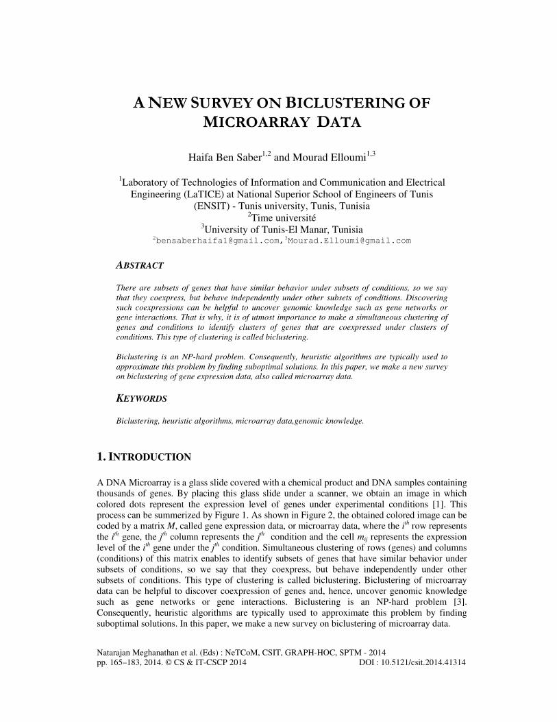
process can be summerized by Figure 1. As shown in Figure 2, the obtained colored image can be
coded by a matrix M, called gene expression data, or microarray data, where the ith row represents
the ith gene, the jth column represents the jth condition and the cell mij represents the expression
level of the ith gene under the j
th condition. Simultaneous clustering of rows (genes) and columns
(conditions) of this matrix enables to identify subsets of genes that have similar behavior under
subsets of conditions, so we say that they coexpress, but behave independently under other
subsets of conditions. This type of clustering is called biclustering. Biclustering of microarray
data can be helpful to discover coexpression of genes and, hence, uncover genomic knowledge
such as gene networks or gene interactions. Biclustering is an NP-hard problem [3].
Consequently, heuristic algorithms are typically used to approximate this problem by finding
suboptimal solutions. In this paper, we make a new survey on biclustering of microarray data.
166 Computer Science & Information Technology (CS & IT)
In this paper, we make a survey on biclustering of gene expression data. The rest of the paper is
organized as follows: First, we introduce some definitions related to biclustering of microarray
data. Then, we present in section 3 some evaluation functions and biclustering algorithms. Next,
we show how to validate biclusters via biclustering tools on microarrays datasets. Finally, we
present our conclusion.
Figure 1. Generation from a DNA microarray of an image where colored dots represent the expression level
of genes under experimental conditions [2]
Figure 2. Coding of the generated colored image to a microarray data
2. BICLUSTERING OF MICROARRAY DATA
Let introduce some definitions related to a biclustering of microarray data [3].
Biclusters : Let I = {1,2,...,n} be a set of indices of n genes, I = {1,2,...,m} be a set of indices of
m conditions and M(I,J) be a data matrix associated with I and J. A bicluster associated with the
data matrix M(I,J) is a couple M(I’,J’) such that II ⊆' and JJ ⊆' .
Computer Science & Information Technology (CS & IT) 167
Types of biclusters : A bicluster can be one of the following cases:
• Bicluster with constant values on rows:
where c is a constant and ai is the adjustment for the row i.
• Bicluster with constant values on columns:
where bj is the adjustment for the column j.
• Bicluster with coherent values: There are two types of biclusters with coherent values. Those
with additive model and those with multiplicative model defined respectively by:
Those with additive model:
And those with multiplicative model:
• Bicluster with coherent evolution: It is a bicluster where all the rows (resp. columns) induce a
linear order across a subset of columns (resp. rows).
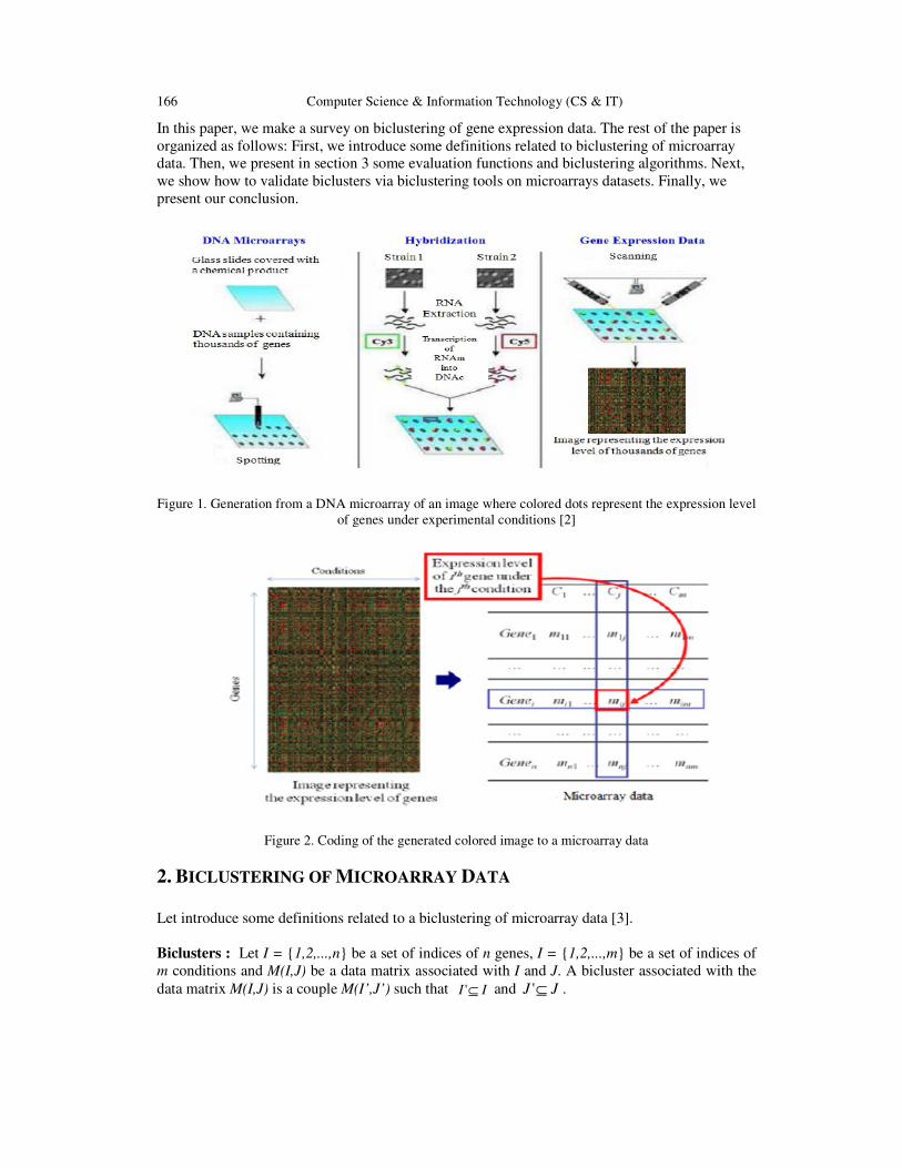
Groups of biclusters : A group of biclusters can be one of the following types [4]:
1. Single bicluster (Figure 3. (a)),
Figure 3.Types of groups of biclusters
168 Computer Science & Information Technology (CS & IT)
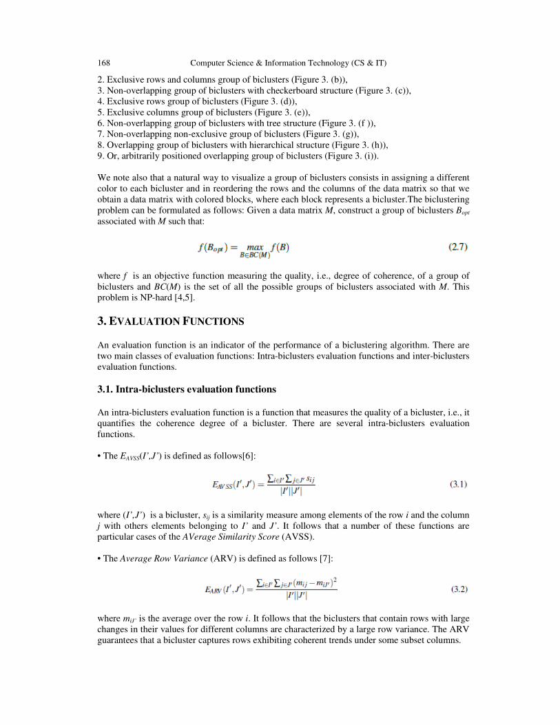
2. Exclusive rows and columns group of biclusters (Figure 3. (b)),
3. Non-overlapping group of biclusters with checkerboard structure (Figure 3. (c)),
4. Exclusive rows group of biclusters (Figure 3. (d)),
5. Exclusive columns group of biclusters (Figure 3. (e)),
6. Non-overlapping group of biclusters with tree structure (Figure 3. (f )),
7. Non-overlapping non-exclusive group of biclusters (Figure 3. (g)),
8. Overlapping group of biclusters with hierarchical structure (Figure 3. (h)),
9. Or, arbitrarily positioned overlapping group of biclusters (Figure 3. (i)).
We note also that a natural way to visualize a group of biclusters consists in assigning a different
color to each bicluster and in reordering the rows and the columns of the data matrix so that we
obtain a data matrix with colored blocks, where each block represents a bicluster.The biclustering
problem can be formulated as follows: Given a data matrix M, construct a group of biclusters Bopt
associated with M such that:
where f is an objective function measuring the quality, i.e., degree of coherence, of a group of
biclusters and BC(M) is the set of all the possible groups of biclusters associated with M. This
problem is NP-hard [4,5].
3. EVALUATION FUNCTIONS An evaluation function is an indicator of the performance of a biclustering algorithm. There are
two main classes of evaluation functions: Intra-biclusters evaluation functions and inter-biclusters
evaluation functions.
3.1. Intra-biclusters evaluation functions
An intra-biclusters evaluation function is a function that measures the quality of a bicluster, i.e., it
quantifies the coherence degree of a bicluster. There are several intra-biclusters evaluation
functions.
• The EAVSS(I’,J’) is defined as follows[6]:
where (I’,J’) is a bicluster, sij is a similarity measure among elements of the row i and the column
j with others elements belonging to I’ and J’. It follows that a number of these functions are
particular cases of the AVerage Similarity Score (AVSS).
• The Average Row Variance (ARV) is defined as follows [7]:
where miJ’ is the average over the row i. It follows that the biclusters that contain rows with large
changes in their values for different columns are characterized by a large row variance. The ARV
guarantees that a bicluster captures rows exhibiting coherent trends under some subset columns.

Computer Science & Information Technology (CS & IT) 169
• The Mean Squared Residue (MSR) is defined as follows [8]:
where mI’J’ is the average over the whole bicluster, mI’ j is the average over the column j, miJ’ is the
average over the row i. The EMSR represents the variation associated with the interaction between
the rows and the columns in the bicluster. It follows that a low (resp. high) EMSR value, i.e., close
to 0 (resp. higher than a fixed threshold d), indicates that the bicluster is strongly (resp. weakly)
coherent. The EMSR function is inadequate to assess certain types of biclusters. For example, the
EMSR function is good for biclusters of coherent values with additive model but not for coherent
values with multiplicative model.
• The Volume (V) is defined as follows [7]:
This function enables to have the maximum-sized bicluster that does not exceed a certain
coherence value expressed as a MSR score. EV(I’,J’) finds the maximum-sized bicluster that does
not exceed a certain coherence value [9] expressed as a MSR score. Hence, discovered biclusters
have a high EV(I’,J’) maximized and lower EMSR than a given threshold 0≥δ .
• The Mean Square Error (MSE) is defined as follows [10]:
where mIJ is the average over the whole matrix, mI j is the average over the column j of the whole
matrix and miJ’ is the average over the row i. This function identifies constant biclusters.
• The Average Correlation Value (ACV) is defined as follows [5, 11]:
where rij )( ji ≠ (resp. rkl )( lk ≠ ) is the Pearson’s correlation coefficient associated with the row
indices i and j (resp. k and l) in the bicluster (J’,J’) [8]. The values of EACV belong to [0;1], hence,
a high (resp. low) EACV value, i.e., close to 1 (resp. close to 0), indicates that the bicluster is
strongly (resp. weakly) coherent. However, the performance of the EACV function decreases when
noise exists in the data matrix [5, 11].
• The Average Spearman’s Rho (ASR) is defined as follows [2]:
where )( jiij
≠ρ (resp. )( lkKL
≠ρ ) is the Spearman’s rank correlation associated with the row
indices i and j in the bicluster (I’,J’) [12], The values of the EASR function belong also to [-1,1],
170 Computer Science & Information Technology (CS & IT)
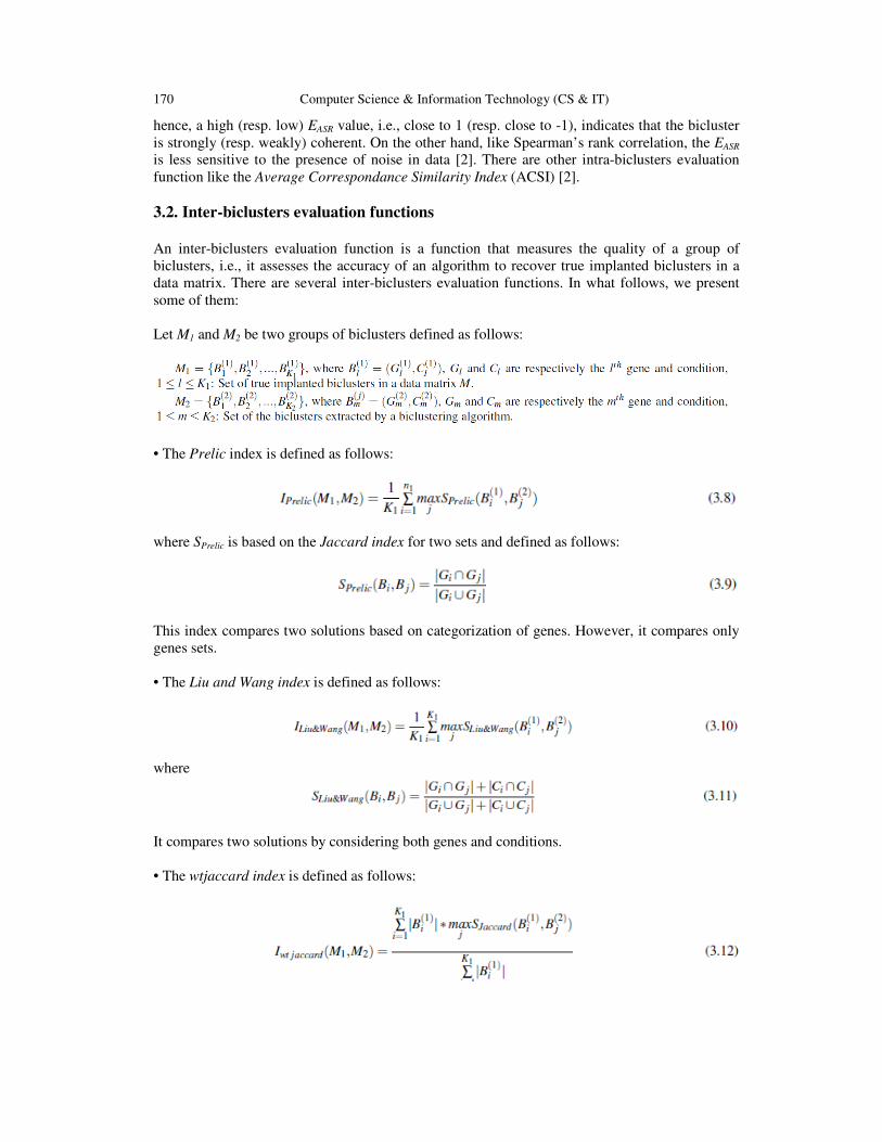
hence, a high (resp. low) EASR value, i.e., close to 1 (resp. close to -1), indicates that the bicluster
is strongly (resp. weakly) coherent. On the other hand, like Spearman’s rank correlation, the EASR
is less sensitive to the presence of noise in data [2]. There are other intra-biclusters evaluation
function like the Average Correspondance Similarity Index (ACSI) [2].
3.2. Inter-biclusters evaluation functions
An inter-biclusters evaluation function is a function that measures the quality of a group of
biclusters, i.e., it assesses the accuracy of an algorithm to recover true implanted biclusters in a
data matrix. There are several inter-biclusters evaluation functions. In what follows, we present
some of them:
Let M1 and M2 be two groups of biclusters defined as follows:
• The Prelic index is defined as follows:
where SPrelic is based on the Jaccard index for two sets and defined as follows:
This index compares two solutions based on categorization of genes. However, it compares only
genes sets.
• The Liu and Wang index is defined as follows:
where
It compares two solutions by considering both genes and conditions.
• The wtjaccard index is defined as follows:

Computer Science & Information Technology (CS & IT) 171
Where
• The Dice index is defined as follows:
where:
which is proposed in [13] and called F-measure in biclustering cases to computes the overall
relevance of two bicluster solutions.
• The Santamaría index is defined as follows:
The Santamaría index is the most conservative index among above others indices and used for
biclustering case [14, 13]. In fact, while the Prelic index compares only object sets and the LW
index compares object sets and feature sets independently, the Santamaría index compares two
solutions using pairs of genes and conditions.
For gene expression case, the Gene Match Score (GMS) function doesn’t take into account
column match. It is given by:
where B1 and B2 are two groups of biclusters and the pair (I,J) represents the submatrix whose
rows and columns are given by the set I and J, respectively.
The Row and Column Match Scores (RCMS) assess the method’s accuracy to recover known
biclusters and reveal true ones. Thereafter, more similar measures of match scores have been
introduced [5, 15, 6]. For instance, the evaluation functions, herein called Row and Column
Match Scores, ERCMS1 and ERCMS2, are proposed in [6] and [15], respectively and given by:

172 Computer Science & Information Technology (CS & IT)
All these measures of match score are used to assess the accuracy of an algorithm to recover
known biclusters and reveal true ones. Both ERCMS1 and ERCMS2 have the advantage of reflecting,
simultaneously, the match of the row and column dimensions between biclusters as opposed to
EGMS that doesn’t take into account column match. They vary between 0 and 1 (the higher the
better the accuracy). Let Bopt denote the set of true implanted biclusters in the data matrix M and B
the set of the output biclusters of a biclustering algorithm. Thus, EGMS(Bopt,B) and ERCMS1 (Bopt,B)
express how well each of the true biclusters are detected by the algorithm under consideration.
ERCMS2 (BX,BY), where BX (resp. BY) denotes the set of biclusters detected by the algorithm X (resp.
Algorithm Y), has the particularity to allow the quantification of how well each bicluster
identified by the algorithm X is contained into some bicluster detected by the algorithm Y.
4. BICLUSTERING ALGORITHMS As we mentioned earlier, the biclustering problem is NP-hard [3, 10]. Consequently, heuristic
algorithms are typically used to approximate the problem by finding suboptimal solutions. We
distinguish different approaches adopted by biclustering approaches[3].
4.1. Iterative Row and Column Clustering Combination Approach
By adopting the Iterative Row and Column Clustering Combination Approach (IRCCC)
approach, we apply clustering algorithms on both rows and columns separately and then combine
the results to obtain biclusters [56]. Table 5 is a synoptic table of biclustering algorithms adopting
IRCCC approach. The conceptually simpler way to perform biclustering using existing
algorithms without searching novels algorithms. But, this approach consider approximatively
same advantages and drawbacks that clustering algorithms used. Among the algorithms adopting
this approach we mention Croki2 [58], Crobin [58], DCC [59], ITWC [61], CTWC [54] and Bi-
SOM [60].
Table 1. Biclustering algorithms adopting IRCCC approach.
Algorithms
Bicluster
discovery
Types of
biclusters
Types of groups
of biclusters
Data type Time complexity
Croeuc [57]
Coherent values
–
One at time
Continuous
–
Croki2 [58] Coherent values – One at time
Continuous
–
CroBin[57] Coherent values – One at time
Continuous
–
CemCroki [57] Coherent values – One at time
Continuous
–
DCC [59] Coherent values Exclusive
dimension
One at time
Continuous
–
Bi-SOM [60] Coherent values – - –
ITWC [61] Coherent values – One at time
Continuous
–
CTWC[54] Constant columns Arbitrarily
positioned
overlapping
One at time
Continuous
–
Computer Science & Information Technology (CS & IT) 173
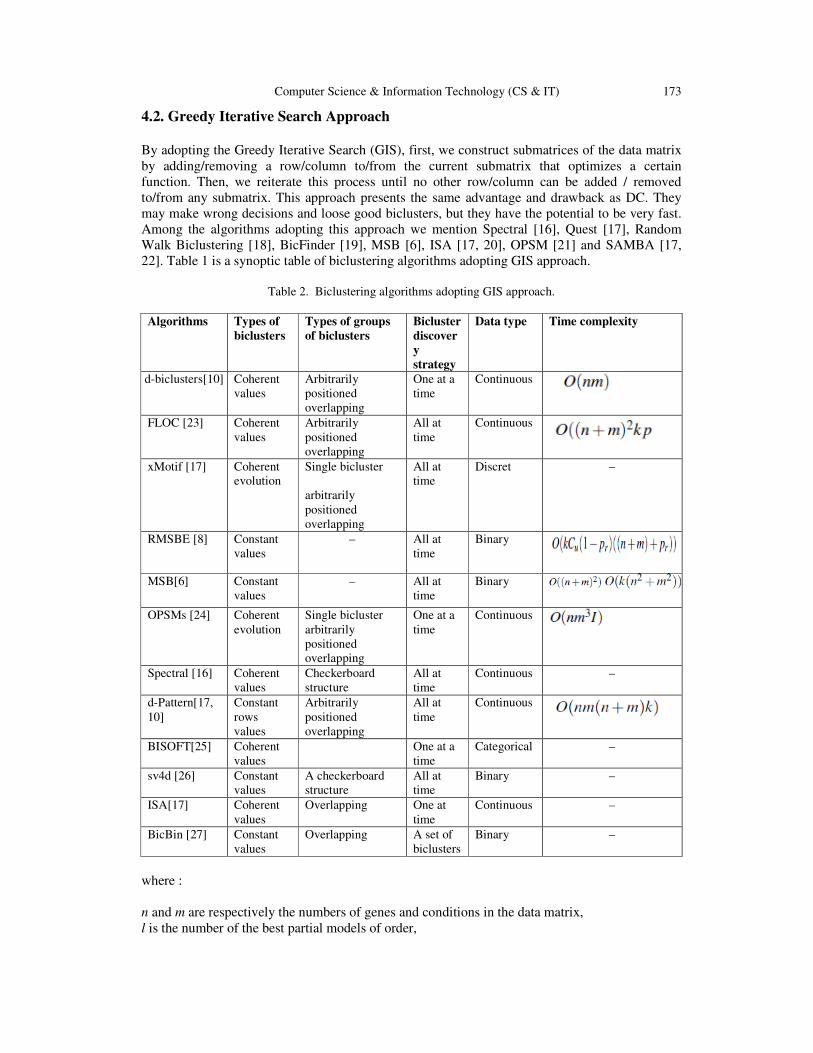
4.2. Greedy Iterative Search Approach
By adopting the Greedy Iterative Search (GIS), first, we construct submatrices of the data matrix
by adding/removing a row/column to/from the current submatrix that optimizes a certain
function. Then, we reiterate this process until no other row/column can be added / removed
to/from any submatrix. This approach presents the same advantage and drawback as DC. They
may make wrong decisions and loose good biclusters, but they have the potential to be very fast.
Among the algorithms adopting this approach we mention Spectral [16], Quest [17], Random
Walk Biclustering [18], BicFinder [19], MSB [6], ISA [17, 20], OPSM [21] and SAMBA [17,
22]. Table 1 is a synoptic table of biclustering algorithms adopting GIS approach.
Table 2. Biclustering algorithms adopting GIS approach.
Algorithms Types of
biclusters
Types of groups
of biclusters
Bicluster
discover
y
strategy
Data type Time complexity
d-biclusters[10] Coherent
values
Arbitrarily
positioned
overlapping
One at a
time
Continuous
FLOC [23] Coherent
values
Arbitrarily
positioned
overlapping
All at
time
Continuous
xMotif [17] Coherent
evolution
Single bicluster
arbitrarily
positioned
overlapping
All at
time
Discret –
RMSBE [8] Constant
values
– All at
time
Binary
MSB[6] Constant
values
– All at
time
Binary
OPSMs [24] Coherent
evolution
Single bicluster
arbitrarily
positioned
overlapping
One at a
time
Continuous
Spectral [16] Coherent
values
Checkerboard
structure
All at
time
Continuous –
d-Pattern[17,
10]
Constant
rows
values
Arbitrarily
positioned
overlapping
All at
time
Continuous
BISOFT[25] Coherent
values
One at a
time
Categorical –
sv4d [26] Constant
values
A checkerboard
structure
All at
time
Binary –
ISA[17] Coherent
values
Overlapping One at
time
Continuous –
BicBin [27] Constant
values
Overlapping A set of
biclusters
Binary –
where :
n and m are respectively the numbers of genes and conditions in the data matrix,
l is the number of the best partial models of order,

174 Computer Science & Information Technology (CS & IT)
K is the maximum number of iterations,
Cu isthe cost of computing the new residue and the new row variance of the bicluster after
performing a move,
pr is a user-provided probability that the algorithm is allowed to execute a random move.
4.3. Exhaustive Bicluster Enumeration Approach
By adopting the Exhaustive Bicluster Enumeration (EBE), We identify all the possible groups of
biclusters in order to keep the best one, i.e., the one that optimizes a certain evaluation function.
The advantage of this approach is that it is able to obtain the best solutions. Its drawback is that it
is costly in computing time and memory space Among the algorithms adopting this approach we
mention BSGP[28, 29], OPC [30, 6], CPB [30], IT[31], e-Bmotif [29], BIMODULE [32], RAP
[26], BBK [33] and MSB [6]. Table 2 is a synoptic table of biclustering algorithms adopting EBE
approach.
Table 3. Biclustering algorithms adopting EBE approach.
Algorith
ms
Types of
biclusters
Types of
groups of
biclusters
Bicluster
discovery
strategy
Data type Time complexity
e-BiMotif
[34][29]
Coherent values – All at time Contingence
CPB [30] Coherent values – All at time Contingence
Categorical
–
OPC [30] Coherent
evolution
Arbitrarily
positioned
overlapping
All at time –
PClusters
[10]
Coherent values Non-
overlapping
non-exclusive
All at time Binary
BSGP
[28, 29]
Coherent values – All at time Contingence
Categorical
–
Expander
[35]
Coherent
evolution
– One a time Categorical –
IT [31] Coherent values – All at time Contingence –
BIMODU
LE [32]
Coherent values – One a time Contingence
Categorical
–
RAP [26] Constant row
values coherent
values
Overlapping One a time Continuous –
SAMBA
[17, 22]
Coherent
evolution
Arbitrarily
positioned
Overlapping
All at time Continuous
MDS[36] – cHawk
[37]
Constant
values//coherent
Evolution
Overlapping All at time Categorial –
BBK[33] Constant values – One at time Binary –
Where
d is the bounded degree of gene vertices in a bipartite graph G whose two sides correspond to he
set of genes and the set of conditions.
r is the maximum weight edge in the bipartite graph G.

Computer Science & Information Technology (CS & IT) 175
4.4. Distribution Parameter Identification Approach
By adopting the Distribution Parameter Identification (DPI) approach use a statistical model to
identify the distribution parameters and generate the data by minimizing a certain criterion
iteratively. These algorithms certainly find the best biclusters, if they exist, but have a very
serious drawback. Due to their high complexity, they can only be executed by assuming
restrictions on the size of the biclusters. Among the algorithms adopting this approach we
mention QUBIC [38], PRMs [39], FABIA [40], BEM [41] and BCEM [42]. Table 3 is a synoptic
table of biclustering algorithms adopting DPI approach.
Table 4. Biclustering algorithms adopting DPI approach.
Algorithms
Bicluster
discovery
Types of
biclusters
Types of
groups of
biclusters
Bicluster
discovery
strategy
Data type Time
complexity
PRMs [43] Coherent
constant
values on
Columns
Arbitrarily
positioned
overlapping
All at time Binary –
iBBiG[44]
Coherent
values
Overlapping One set at
time Binary
Binary –
Plaid[45, 46]
Coherent
values
Arbitrarily
positioned
overlapping
One at time Continuous
QUBIC[38] Constant
columns or
rows
Exclusive
dimension
One at time Discrete –
FABIA[40] Constant
values
Overlapping All at time Catgeorial
binary
–
BEM [41]
Coherent
values
– All at time Continuous
binary
BCEM[42] Coherent
values
– All at time Continuous
binary
–
ISA [20] Coherent or
constant
values
– One at a
time
Continuous –
Gibbs[47] Constant
columns or
rows
Exclusive
dimension
One at a
time
Catgeorial
binary
–
4.5. Divide and Conquer Approach
By adopting the Divide-and-Conquer (DC) approach, first, we start by a bicluster representing the
whole data matrix then we partition this matrix in two submatrices to obtain two biclusters. Next,
we reiterate recursively this process until we obtain a certain number of biclusters verifying a
specific set of properties. The advantage of DC is that it is fast, its drawback is that it may ignore
good biclusters by partitioning them before identifying them. DC algorithms have the significant
advantage of being potentially very fast. However, they have the very significant drawback of
being likely to miss good biclusters that may be split before they can be identified. Among the
algorithms adopting this approach we mention OWS [48], TWS [49], BiBit [28] and BARTMAP
[50] and GS [51].

176 Computer Science & Information Technology (CS & IT)
Table 5. Biclustering algorithms adopting DC approach.
Algorithms
Bicluster
discovery
Types of
biclusters
Types of groups
of biclusters
Data type Time complexity
Block Clustering
[52]
Constant
values
Non-overlapping
tree structure
Binary
categorial
–
OWS[53] Constant
values
All at time Continuous
TWS [54] Constant
values
All at time Continuous –
BiBit [28] Constant
values
All at time Binary
BiBit [28] Constant
values
All at time Binary –
Cmnk [44] Constant
values
One at time Binary –
GS [51] Constant
values
One at time Binary –
where β is the number of biclusters that are not entirely contained in any other bicluster.
5. BICLUSTERING VALIDATION There are two types of biclusters validation;
(i) Statistical validation: It is used to validate synthetical data
(ii) Biological validation: It is used to validate biological data
5.1. Statistical validation
Statistical validation can be made by adopting one or many of the following indices:
Separation: It reflects how well the biclusters are separated from each other. Separation between
two biclusters
A and B is defined as follows [62]:
Coverage: We distinguish three types of coverage, matrix coverage, genes coverage and
conditions coverage:
Computer Science & Information Technology (CS & IT) 177
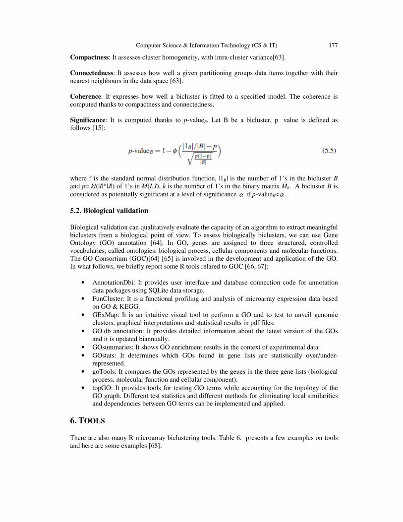
Compactness: It assesses cluster homogeneity, with intra-cluster variance[63].
Connectedness: It assesses how well a given partitioning groups data items together with their
nearest neighbours in the data space [63].
Coherence: It expresses how well a bicluster is fitted to a specified model. The coherence is
computed thanks to compactness and connectedness.
Significance: It is computed thanks to p-valueB. Let B be a bicluster, p�value is defined as
follows [15]:
where f is the standard normal distribution function, |1B| is the number of 1’s in the bicluster B
and p= k/(|I|*|J|) of 1’s in M(I,J), k is the number of 1’s in the binary matrix Mb. A bicluster B is
considered as potentially significant at a level of significance α if p-valueB<α .
5.2. Biological validation
Biological validation can qualitatively evaluate the capacity of an algorithm to extract meaningful
biclusters from a biological point of view. To assess biologically biclusters, we can use Gene
Ontology (GO) annotation [64]. In GO, genes are assigned to three structured, controlled
vocabularies, called ontologies: biological process, cellular components and molecular functions.
The GO Consortium (GOC)[64] [65] is involved in the development and application of the GO.
In what follows, we briefly report some R tools relared to GOC [66, 67]:
• AnnotationDbi: It provides user interface and database connection code for annotation
data packages using SQLite data storage.
• FunCluster: It is a functional profiling and analysis of microarray expression data based
on GO & KEGG.
• GExMap: It is an intuitive visual tool to perform a GO and to test to unveil genomic
clusters, graphical interpretations and statistical results in pdf files.
• GO.db annotation: It provides detailed information about the latest version of the GOs
and it is updated biannually.
• GOsummaries: It shows GO enrichment results in the context of experimental data.
• GOstats: It determines which GOs found in gene lists are statistically over/under-
represented.
• goTools: It compares the GOs represented by the genes in the three gene lists (biological
process, molecular function and cellular component).
• topGO: It provides tools for testing GO terms while accounting for the topology of the
GO graph. Different test statistics and different methods for eliminating local similarities
and dependencies between GO terms can be implemented and applied.
6. TOOLS There are also many R microarray biclustering tools. Table 6. presents a few examples on tools
and here are some examples [68]:

178 Computer Science & Information Technology (CS & IT)
• arules: It is a mining association rules and frequent itemsets. It provides the infrastructure
for representing, manipulating and analyzing transaction data and patterns. It also
provides interfaces of the association mining algorithms Apriori and Eclat [69].
• lattice: It is a high-level data visualization system with an emphasis on multivariate data.
It supports the creation of trellis graphs to display multivariate relationship between
variables, conditioned on one or more other variables via R graphics [69].
• rootSolve: It finds the root of nonlinear functions, solves the steady-state conditions for
uni/multi-component and equilibrium analysis of ordinary differential equations via a
dynamically running; like gradient and Jacobian matrices, non-linear equations by the
Newton-Raphson algorithm.
Table 6. Tools used to evaluate and compare biclustering algorithms
Tool Biclustering algorithms Reference
Lattice Galois lattice [17]
arules rules [71]
rootSolve, pracma Newton Raphson [71]
blockcluster Coclustering [17]
biclustGUI CC, Plaid, BiMAX„ xMOTIFs, xQuest,
Spectral, FABIA, ISA
[20]
biclust Plaid, BiMAX, xMOTIFs, xQuest, Spectral [17]
BcDiag biclust, eisa, isa2 [17]
FABIA, FABIAs,
FABIAp,
FABIA [40]
NMF NMF [70]
s4vd s4vd [26]
qubic Rqubic [38]
eisa, isa2 ISA [17]
BicARE FLOC [72]
ThreeWayPlaid Plaid for three-dimensional data [46]
IBBigs iBBiG [44]
Superbiclust Ensemble Biclustering [73, 41]
HSSVD HSSVD [46]
FacPad Factor analysis for pathways [45]
FastICA Fast independent component analysis [74]
CMonkey cMonkey [75]
• pracma: It root finds through Newton-Raphson or Secant algorithms [70] via using
functions from numerical analysis and linear algebra, numerical optimization, differential
equations and some special functions. It also uses Matlab function names where
appropriate to simplify porting.
• BicARE: It is based on the FLOC algorithm [23] for biclustering analysis and results
exploration.
• BcDiag: It provides methods for data pre-processing, visualization, and statistical
validation to diagnostic and visualize in two-dimensional data based on two way anova
[40] and median polish residual plots for biclust package output obtained from biclust,
eisa-isa2 and fabia packages [17][40]. In addition, the biclust package can be used via
biclustGUI, i.e. R commander plug in.
Computer Science & Information Technology (CS & IT) 179
• blockcluster: It performs coclustering of binary, contingency and categorical datasets
with utility functions to visualize the coclustered data. It contains a function cocluster
which
• performs coclustering and returns object of appropriate class. It also contains coclust
strategy function which returns an object of class strategy.
• rqubic: It represents an implementation of the QUBIC algorithm [38] for the qualitative
biclustering with gene expression data.
• HSSVD: It discovers and compares subgroups of patients and genes which
simultaneously display unusual levels of variability. It detects both mean and variance
biclusters by testing the biclustering with heterogeneous variance.
• iBBig: It optimizes applying binary data analysis to meta-gene set analysis of gene
expression datasets. It extracts iteratively groups of phenotypes from multiple studies that
are associated with similar gene sets without requiring prior knowledge of the number or
scale of clusters and allows discovery of clusters with diverse sizes.
• NMF: It provides a framework to perform Non-negative Matrix Factorization (NMF). It
implements a set of already published algorithms and seeding methods, and provides a
framework to test, develop and plug new/custom algorithms. It performs parallel
computations on multicore machines.
• s4vd: It performs a biclustering via sparse singular value decomposition (svd) with a
nested stability selection. The result is an biclust object and thus all methods of the
biclust package can be applied.
• superbiclust: It generates as a result a number of (or super) biclusters with none or low
overlap from a bicluster set, i.e. ensemble biclustering [42], with respect to the
initialization parameters for a given bicluster solution. The set of robust biclusters is
based on the similarity of its elements, i.e. overlap, and on the hierarchical tree obtained
via cut-off points.
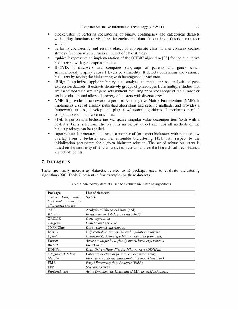
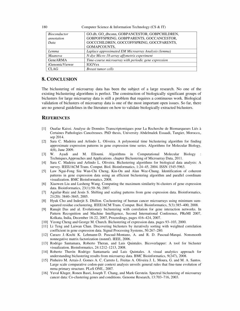
7. DATASETS
There are many microarray datasets, related to R package, used to evaluate biclustering
algorithms [68]. Table 7. presents a few examples on these datasets.
Table 7. Microarray datasets used to evaluate biclustering algorithms
Package List of datasets
aroma. Copy-number
(cn) and aroma. for
affyrmetrix anpuce
Spleen
Abd Analysis of Biological Data (abd)
ICluster Breast cancer, DNA cn, breast.chr17
ORCME Gene expression
Adegenet Genetic and genomic
SNPMClust Dose-response microarray
DCGL Differential co-expression and regulation analysis
Opmdata OmniLog(R) Phenotype Microarray data (opmdata)
Knorm Across multiple biologically interrelated experiments
Biclust BicatYeast
DDHFm Data-Driven Haar-Fisz for Microarrays (DDHFm)
integrativeMEdata Categorical clinical factors, cancer microarray
Madsim Flexible microarray data simulation model (madsim)
EMA Easy Microarray data Analysis (EMA)
FBN SNP microarray
BioConductor Acute Lymphocytic Leukemia (ALL), arrayMissPattern.
180 Computer Science & Information Technology (CS & IT)
Bioconductor
annotation
Data
GO.db, GO_dbconn, GOBPANCESTOR, GOBPCHILDREN,
GOBPOFFSPRING, GOBPPARENTS, GOCCANCESTOR,
GOCCCHILDREN, GOCCOFFSPRING, GOCCPARENTS,
GOMAPCOUNTS,
Lemma Laplace approximated EM Microarray Analysis (lemma)
Maanova N-dye Micro 18-array affymetrix experiment
GeneARMA Time-course microarray with periodic gene expression
iGenomicViewer IGGVex
CLAG Breast tumor cells
8. CONCLUSION
The biclustering of microarray data has been the subject of a large research. No one of the
existing biclustering algorithms is perfect. The construction of biologically significant groups of
biclusters for large microarray data is still a problem that requires a continuous work. Biological
validation of biclusters of microarray data is one of the most important open issues. So far, there
are no general guidelines in the literature on how to validate biologically extracted biclusters.
REFERENCES
[1] Ouafae Kaissi. Analyse de Données Transcriptomiques pour La Recherche de Biomarqueurs Liés à
Certaines Pathologies Cancéreuses. PhD thesis, University Abdelmalek Essaadi, Tangier, Morocco„
sep 2014.
[2] Sara C. Madeira and Arlindo L. Oliveira. A polynomial time biclustering algorithm for finding
approximate expression patterns in gene expression time series. Algorithms for Molecular Biology,
4(8), June 2009.
[3] W. Ayadi and M. Elloumi. Algorithms in Computational Molecular Biology :
Techniques,Approaches and Applications. chapter Biclustering of Microarray Data, 2011.
[4] Sara C. Madeira and Arlindo L. Oliveira. Biclustering algorithms for biological data analysis: A
survey. IEEE/ACM Trans. Comput. Biol. Bioinformatics, 1:24–45, 2004. ISSN 1545-5963.
[5] Law Ngai-Fong Siu Wan-Chi Cheng, Kin-On and Alan Wee-Chung. Identification of coherent
patterns in gene expression data using an efficient biclustering algorithm and parallel coordinate
visualization. BMC Bioinformatics, 2008.
[6] Xiaowen Liu and Lusheng Wang. Computing the maximum similarity bi-clusters of gene expression
data. Bioinformatics, 23(1):50–56, 2007.
[7] Aguilar-Ruiz and Jesús S. Shifting and scaling patterns from gene expression data. Bioinformatics,
21(20): 3840–3845, 2005.
[8] Hyuk Cho and Inderjit S. Dhillon. Coclustering of human cancer microarrays using minimum sum-
squared residue coclustering. IEEE/ACM Trans. Comput. Biol. Bioinformatics, 5(3):385–400, 2008.
[9] Ranajit Das and al. Evolutionary biclustering with correlation for gene interaction networks. In
Pattern Recognition and Machine Intelligence, Second International Conference, PReMI 2007,
Kolkata, India, December 18-22, 2007, Proceedings, pages 416–424, 2007.
[10] Yizong Cheng and George M. Church. Biclustering of expression data. pages 93–103, 2000.
[11] Li Teng and Laiwan Chan. Discovering biclusters by iteratively sorting with weighted correlation
coefficient in gene expression data. Signal Processing Systems, 50:267–280.
[12] Carazo J.-Kochi K. Lehmann-D. Pascual-Montano, A. and R. D. Pascual-Marqui. Nonsmooth
nonnegative matrix factorization (nsnmf). IEEE, 2006.
[13] Rodrigo Santamara, Roberto Theran, and Luis Quintales. Bicoverlapper: A tool for bicluster
visualization. Bioinformatics, 24:1212–1213, 2008.
[14] Roberto Therón Rodrigo Santamaría and Luis Quintales. A visual analytics approach for
understanding biclustering results from microarray data. BMC Bioinformatics, 9(247), 2008.
[15] Pinheiro M. Arrais-J. Gomes A. C. Carreto L. Freitas A. Oliveira J. L. Moura, G. and M. A. Santos.
Large scale comparative codon-pair context analysis unveils general rules that fine-tune evolution of
mrna primary structure. PLoS ONE., 2007.
[16] Yuval Kluger, Ronen Basri, Joseph T. Chang, and Mark Gerstein. Spectral biclustering of microarray
cancer data: Co-clustering genes and conditions. Genome Research, 13:703–716, 2003.

Computer Science & Information Technology (CS & IT) 181
[17] Santamaria R. Khamiakova-T. Sill M. Theron R. Quintales L. Kaiser, S. and F. Leisch. biclust:
Bicluster algorithms. R package., 2011.
[18] Eugenio Cesario Fabrizio Angiulli and Clara Pizzuti. Random walk biclustering for microarray data.
Information Sciences, 178(6):1479–1497, 2008.
[19] Elloumi M. Ayadi, W. and J.-K. Hao. Bicfinder: a biclustering algorithm for microarray data analysis.
Knowledge and Information Systems., 2012.
[20] Jan Ihmels, Sven Bergmann, and Naama Barkai. Defining transcription modules using large-scale
gene expression data. Bioinformatics, 20(13):1993–2003, 2004.
[21] Chor B.-Karp R. Ben-Dor, A. and Z. Yakhini. Clustering gene expression patterns. 6, 2002.
[22] Amos Tanay, Roded Sharan, and Ron Shamir. Discovering statistically significant biclusters in gene
expression data. In In Proceedings of ISMB 2002, pages 136–144, 2002.
[23] Jiong Yang and al. Enhanced biclustering on expression data.
[24] Chor Benny Karp Richard Ben-Dor, Amir. and Zohar. Yakhini. Discovering local structure in gene
expression data: The order-preserving submatrix problem. In Proceedings of the Sixth Annual
International Conference on Computational Biology, RECOMB ’02, pages 49–57, New York, NY,
USA, 2002. ACM.
[25] Hossam S. Sharara and Mohamed A. Ismail. Bisoft: A semi-fuzzy approach for biclustering gene
expression data. In BIOCOMP, 2008.
[26] Martin Sill, Sebastian Kaiser, Axel Benner, and Annette Kopp-Schneider. Robust biclustering by
sparse singular value decomposition incorporating stability selection. Bioinformatics, 27:2089–2097,
2011.
[27] Miranda van Uitert, Wouter Meuleman, and Lodewyk F. A. Wessels. Biclustering sparse binary
genomic data. Journal of Computational Biology, 15(10):1329–1345, 2008.
[28] Perez-Pulido A. J. Rodriguez-Baena, D. S. and J.S. Aguilara-Ruiz. A biclustering algorithm for
extracting bit-patterns from binary datasets. Bioinformatics., 2011.
[29] Elloumi M. Ayadi, W. and J.-K. Hao. A biclustering algorithm based on a bicluster enumeration tree:
application to dna microarray data. BioData Mining., 2009.
[30] Tze-Haw Huang ; XingXing Song ; Mao Lin Huang. Optimized data acquisition by time series
clustering in opc. IEEE., 2011.
[31] Inderjit S. Dhillon, Subramanyam Mallela, and Dharmendra S. Modha. Information-theoretic co-
clustering. In Proceedings of the ninth ACM SIGKDD international conference on Knowledge
discovery and data mining, pages 89–98. ACM Press, 2003.
[32] Jiun-Rung Chen and Ye-In Chang. A condition-enumeration tree method for mining biclusters from
dna microarray data sets. Elsevier, 97:44–59, 2007.
[33] Stefan Bleuler Oliver Voggenreiter and Wilhelm Gruissem. Exact biclustering algorithm for the
analysis of large gene expression data sets. Eighth International Society for Computational Biology
(ISCB) Student Council Symposium Long Beach, CA, USA.July, pages 13–14, 2012.
[34] Joana P. Gonalves and Sara C. Madeira. e-bimotif: Combining sequence alignment and biclustering to
unravel structured motifs. In IWPACBB, volume 74, pages 181–191, 2010.
[35] Shamir and al. Expander - an integrative program suite for microarray data analysis. BMC
Bioinformatics, 6: 232, 2005.
[36] Dong Wang and al. Mapping query to semantic concepts: Leveraging semantic indices for automatic
and interactive video retrieval. In ICSC ’07: Proceedings of the International Conference on Semantic
Computing, pages 313–320, 2007.
[37] W. Ahmad. chawk: An efficient biclustering algorithm based on bipartite graph crossing
minimization. 2007.
[38] Haibao Tang Andrew H. Paterson Guojun Li, Qin Ma and Ying Xu. Qubic: a qualitative biclustering
algorithm for analyses of gene expression data. 2009.
[39] Nir Friedman, Lise Getoor, Daphne Koller, and Avi Pfeffer. Learning probabilistic relational models.
In IJCAI, pages 1300–1309, 1999.
[40] Sepp Hochreiter, Ulrich Bodenhofer, Martin Heusel, Andreas Mayr, Andreas Mitterecker, Adetayo
Kasim, Tatsiana Khamiakova, Suzy Van Sanden, Dan Lin 0004, Willem Talloen, Luc Bijnens,
Hinrich W. H. Göhlmann, Ziv Shkedy, and Djork-Arné Clevert. Fabia: factor analysis for bicluster
acquisition. Bioinformatics, 26(12):1520–1527, 2010.
[41] Mohamed Nadif and Gérard Govaert. Block clustering via the block gem and two-way em algorithms.
In AICCSA’05, pages –1–1, 2005.
[42] Mohamed Nadif and Gerard Govaert. A comparison between block cem and two-way cem algorithms
to cluster a contingency table. In PKDD’05, pages 609–616, 2005.
182 Computer Science & Information Technology (CS & IT)
[43] Baocheng W. Guifen, C. and Y. Helong. The implementation of parallel genetic algorithm based on
matlab. Advanced Parallel Processing Technologies., 2007.
[44] Daniel Gusenleitner, Eleanor Howe, Stefan Bentink, John Quackenbush, and Aedin C. Culhane.
ibbig: iterative binary bi-clustering of gene sets. Bioinformatics, 28(19):2484–2492, 2012.
[45] Lazzeroni and Owen. Plaid models for gene expression data. Statistica Sinica., 2002.
[46] Shawn Mankad and George Michailidis. Biclustering three-dimensional data arrays with plaid
models. Journal of Computational and Graphical Statistics, 2013.
[47] Ole Andreatta, Massimo Lund and Morten Nielsen. Simultaneous alignment and clustering of peptide
data using a gibbs sampling approach. Bioinformatics, 29(1):8–14, 2013.
[48] Hartigan. Clustering Algorithms, chapter Direct splitting. 1975.
[49] Gerard GOVAERT. La classification croisee. Modulad, 1983.
[50] Wunsch II Xu, Rui and Donald C. Bartmap: A viable structure for biclustering. Neural Netw.,
24:709–716, September, 2011.
[51] Douglas Creighton Saeid Nahavandi. Thanh Nguyen, Abbas Khosravi. Spike sorting using locality
preserving projection with gap statistics and landmark-based spectral clustering. Neuroscience
Methods., 2014.
[52] I. Llatas, A.J. Quiroz, and J.M. Renom. A fast permutation-based algorithm for block clustering. Test,
6(2): 397–418, 1997.
[53] G. Govaert and M. Nadif. Co-Clustering. FOCUS Series. Wiley, 2013.
[54] G. Getz, E. Levine, and E. Domany. Coupled two-way clustering analysis of gene microarray data.
Proc. Natl. Acad. Sci. USA, 97:12079–12084, 2000.
[55] Amela Preli´c, Stefan Bleuler, Philip Zimmermann, Anja Wille, Peter Bühlmann, Wilhelm Gruissem,
Lars Hennig, Lothar Thiele, and Eckart Zitzler. A systematic comparison and evaluation of
biclustering methods for gene expression data. Bioinformatics, 22:1122–1129, 2006.
[56] J. Caldas and S. Kaski. Hierarchical generative biclustering for microrna expression analysis.
Computational Biology., 2011.
[57] M. Charrad. Une approche gnrique pour l-analyse croisant contenu et usage des sites web par des
methodes de bipartitionnement. PhD thesis, Paris and ENSI, University of Manouba, 2010.
[58] Yves Lechevallier Malika Charrad, Gilbert Saporta, and Mohamed Ben Ahmed. Determination du
nombre des classes dans l’algorithme croki de classification croisee. In EGC’09, pages 447–448,
2009.
[59] Stanislav Busygin and al. Double conjugated clustering applied to leukemia microarray data. 2002.
[60] Khalid Benabdeslem and Kais Allab. Bi-clustering continuous data with self-organizing map. Neural
Computing and Applications, 22(7):1551–1562, 2013.
[61] Chun Tang, Li Zhang 0008, Aidong Zhang, and Murali Ramanathan. Interrelated two-way clustering:
An unsupervised approach for gene expression data analysis. pages 41–48, 2001.
[62] Eleni Mina. Applying biclustering to understand the molecular basis of phenotypic diversity. Phd.
Utrecht University Faculty of Science Department of Information and Computing Sciences, 2011.
[63] Akdes Serin. Biclustering analysis for large scale data. Phd., 2011.
[64] Michael Ashburner. Gene ontology: tool for the unification of biology. Nature Genetics 25, pages 25
–29, 2000.
[65] Gene ontology consortium. Internet:, . URL http://www.geneontology.org/,note= September2014.
[66] Pietro Hiram Guzzi, Marianna Milano, and Mario Cannataro. Mining association rules from gene
ontology and protein networks: Promises and challenges. Procedia Computer Science, 29(0):1970 –
1980, 2014. International Conference on Computational Science.
[67] Xuebo Song, Lin Li, Pradip K. Srimani, Philip S. Yu, and James Z.Wang. Measure the semantic
similarity of go terms using aggregate information content. IEEE/ACM Trans. Comput. Biol.
Bioinformatics, 11:468–476, 2014.
[68] Cran package. Internet:, . URL http://cran.r-project.org/web/packages. July 2014.
[69] Kuznetsov S. O. Macko J. Jr. W. M. Kaytoue, M. and A. Napoli. Mining biclusters of similar values
with triadic concept analysis. The Eighth International Conference on Concept Lattices and Their
Applications., 2011.
[70] Chris H. Q. Ding, Tao Li, and Wei Peng. Nonnegative matrix factorization and probabilistic latent
semantic indexing: Equivalence chi-square statistic, and a hybrid method. In AAAI’06, 2006.
[71] Haifa BenSaber. Classification non supervisiee des donnees des puces a ADN", ESSTT. 2010.
[72] Jiong Yang, HaixunWang,WeiWang 0010, and Philip S. Yu. An improved biclustering method for
analyzing gene expression profiles. International Journal on Artificial Intelligence Tools, 14(5):771–
790, 2005.

Computer Science & Information Technology (CS & IT) 183
[73] Mehmet Koyuturk. Using protein interaction networks to understand complex diseases. Computer,
45(3): 31–38, 2012.
[74] C Heaton J L Marchini and B D Ripley. fastica: Fastica algorithms to perform ica and projection
pursuit. R package, 2013.
[75] Baliga N. S. Reiss, D. J. and Bonneau. cmonkey integrated biclustering algorithm. R package, 2012.
AUTHORS Professor ELLOUMI Mourad : Full Professor in Computer Science Head of the
BioInformatics Group (BIG) of The Laboratory of Technologies of Information and
Communication, and Electrical Engineering (LaTICE), National High School of
Engineers of T unis (ENSIT), University of Tunis, Tunisia, and Professor at the Faculty of
Economic Sciences and Management of Tunis (FSEGT), University of Tunis El Manar,
Tunisia.
Mrs BEN SABER Haifa : Phd student on the BioInformatics Group (BIG) of The
Laboratory of Technologies of Information and Communication, and Electrical
Engineering (LaTICE), National High School of Engineers of Tunis (ENSIT), University
of Tunis, Tunisia, and Assistant at the Time Université, Tunisia.