European Journal of Engineering and Technology Vol. 5 No. 1, 2017 ISSN 2056-5860
Progressive Academic Publishing, UK Page 1 www.idpublications.org
A MATHEMATICAL MODEL TO PREDICT BACK PRESSURE USING
CONSTANT BOTTOM HOLE PRESSURE TECHNIQUE IN MANAGED
PRESSURE DRILLING
Nsikak M. Marcus
University of Port Harcourt
NIGERIA
Boniface A. Oriji
University of Port Harcourt
NIGERIA
ABSTRACT
Drilling through narrow mud window sections using conventional drilling method has been very
challenging as it could easily lead to drilling hazards such as; lost circulation, kick, borehole
instability etc, thereby causing an increase in Non Productive time (NPT). Managed Pressure
Drilling (MPD) is a drilling technology that can be used to precisely control the wellbore annular
pressure profile so as to mitigate drilling hazards and eliminate NPT. In this study, back pressure
was estimated using the pore pressure, hydrostatic pressure and the Annular Frictional Pressure
Loss (AFPL) at various hole intervals using the Constant Bottom Hole Pressure (CBHP) technique
of MPD. A Mathematical model was developed to predict backpressure as a function of the Bottom
Hole Circulating Pressure (BHCP). Three regression models (linear, quadratic and cubic) were
developed for the 12 1/4" and 8 1/2" hole sections respectively from the initial accurately estimated
values of back pressure for these intervals. The models were validated with actual field data from a
typical MPD well in West Africa. The quadratic regression model gave the best approximation for
the two hole sections with an 81% accuracy for the 12 1/4" hole section and a 91% accuracy for the
8 1/2" hole section. These developed models provide an easy and efficient means of predicting back
pressure from the BHCP and also the Equivalent Circulating Density (ECD) for MPD operations.
Keywords: Managed Pressure Drilling, Rheological Models, Backpressure, Regression Analysis.
INTRODUCTION
Discoveries have shown that Non Productive Time (NPT) account for approximately 20% of total
rig time and can be much higher in difficult and complex terrains. Rig rates are on the high, with
some rigs going for as high as 1 million USD per day. During drilling, a range of mud weight is
always given, when the mud weight is higher than the window, there is all tendency that there will
be a higher overbalance pressure which will result to lost circulation that may ultimately lead to
stuck pipe. Also, when the mud weight is outside the window, it results to a negative overbalance
which also leads to drilling problems. To drill safely it is advisable to operate within the mud
window. Most deep water formations have a very small drilling window because of the abnormally
high formation pressure and a low fracture pressure which is caused by rapid sedimentation, lack of
compaction and the low overburden due to the large column of water which is less dense than solid
sediments. Hence, drilling deep water prospects by conventional method is almost not feasible
(Malloy 2007). Drilling in deepwater formations using the conventional drilling technique requires
setting of numerous casing strings at relatively shallow depths in order to prevent lost circulation.
Managed Pressure Drilling (MPD) helps in controlling this problem by drilling with a controlled
BHP. In mature fields, the formation pore pressure, the fracture pressure, the collapse pressure and
the overburden pressure profiles are constantly changing due to production and depletion. This
makes the pressure window narrower, thereby making drilling within the boundary more
challenging without experiencing kicks or lost circulation (Malloy and MacDonald 2008). MPD is
very effective in reducing NPT that are drilling related as it combines new technology with older

European Journal of Engineering and Technology Vol. 5 No. 1, 2017 ISSN 2056-5860
Progressive Academic Publishing, UK Page 2 www.idpublications.org
principles and techniques to manage common drilling problems. According to the International
Association of Drilling Contractors (IADC), Managed Pressure Drilling is an adaptive drilling
process that is used to precisely control the annular pressure profile throughout the wellbore. It's an
advanced form of well control where a closed and pressurized mud system is applied to enable a
more precise control of wellbore pressure profiles than just mud hydrostatic and the pump pressure
adjustments. Estimating the required back pressure term is very important to achieve a successful
MPD operation. Hence, it is very necessary to have a very reliable tool for estimating the required
back pressure. This study aimed at applying the concepts of Constant Bottom hole Pressure (CBHP)
method of managed pressure drilling to develop and validate mathematical models that can
accurately estimate the backpressure required to mitigate drilling hazards for various hole sections
using regression analysis.
LITERATURE REVIEW
According to Rehm et al (2008) new drilling techniques simply combine new methods and the
historical methods to effectively mitigate drilling hazards. Demirdal and Cunha (2007) carried out
some experimental analysis to ascertain the best fluid rheological model for HPHT condition (40 to
2800F and 500 to 12000psi) using un-weighted n-paraffin base drilling fluid (synthetic mud) in
MPD operations. They compared the Bingham plastic, Power law and Yield power law models to
their experimental findings. The yield power law gave the most accurate result when compared to
the experimental result. They modeled the effect of temperature and pressure on drilling fluid
density. Malloy and MacDonald (2008) compared and contrasted conventional, underbalanced and
managed pressure drilling. Their comparison was based on planning objectives, equipment,
operation and well control. They stated that MPD was mainly used to drill wells that are impossible
or uneconomical to drill using the conventional overbalanced drilling technique and that MPD is a
technology for the mitigation of drilling hazards. They concluded that the MPD and underbalanced
drilling are quite different technologies as against the misconception that they are the same. Glen-
Ole et al (2012) stated that the automation of the choke manifold for an MPD system was achieved
with a control system that consists of two main parts, namely; a hydraulic model which was used
for computing real time downhole pressure which in turn controls the choke pressure and a
feedback control algorithm which automatically controls the choke manifold to enable it maintain
the desired choke pressure. They stated further that the hydraulics model determines the accuracy of
the MPD system. They developed a simplified hydraulics model called the fit-for-purpose
hydraulics model for computing the downhole pressures and to provide a choke pressure set point
for automated MPD systems. Jan et al (2014) carried a study to know how pressure control was
affected and sometimes limited by the actual available data and its quality, equipment, hydraulic
models, control algorithm and downhole condition during MPD operations in ERD wells. They
carried out some simulations and showed how the sensor response and bandwidth affected the
ability to accurately control downhole pressures in ERD wells. They concluded that special care
should be taken when applying MPD in ERD wells because, ERD wells are more complex and
challenging when compared to shorter wells. Fan et al (2014) carried out a study on Herschel
Buckley model and came up with a new model by modifying the Herschel Buckley model. They
obtained an explicit equation between the wall shear stress and the volumetric flow rate for pipe and
annular flow from Herschel Buckley fluid model. They were also able to establish a new relation
for pipe and annular Reynolds number and frictional pressure drop. They validated the new model
using well data from Sichuan Basin and they concluded that the new model predicted and calculated
hydraulics more accurately than the other traditional models previously used in MPD operations.
Kinik et al (2015) carried out a simulation analysis for kick detection, control and circulation using
MPD. They were able to highlight the benefits of automated influx detection and control using
MPD system compared to a conventional well control method. Their simulations successfully

European Journal of Engineering and Technology Vol. 5 No. 1, 2017 ISSN 2056-5860
Progressive Academic Publishing, UK Page 3 www.idpublications.org
detected and controlled a gas influx in oil based mud while drilling in onshore western Canada.
They concluded that the current MPD system has the potential for drilling formations with narrow
pressure margins through their accuracy and precision in pressure control and early kick detection.
Hannegan (2010) stated that in reactive MPD, a conventional-wisdom well construction and fluids
program is planned, but the rig is equipped with at least an RCD, choke, and drillstring float(s) as a
means to more safely and efficiently deal with unexpected downhole pressure environment limits.
Medley and Reynolds (2006) stated that the reactive MPD has been implemented on potential
problem wells for years, but very few proactive applications were seen until recently, as the need
for drilling alternatives increased. Aadnoy (2009) stated that the shift from reactive to proactive
MPD requires that the wells be preplanned more thoroughly, but the benefits to the drilling program
typically more than offset the cost of the additional MPD engineering and project management.
Hannegan (2006) stated that MPD has been proven to enable drilling of what might otherwise be
economically un-drillable prospects and that MPD was well on its way to becoming the status quo
technology over the next decade due to the fact that it increased recoverable assets. He discussed
the following variations of MPD; Constant Bottom Hole Pressure (CBHP) technique, Pressurized
Mud Cap Drilling (PMCD) technique, Dual Gradient (DG) technique, Return Flow Control (RFC)
technique and the Reverse Circulation (RC) technique. Some other application of MPD includes;
depleted reservoir drilling, methane hydrates drilling, High pressure High temperature drilling and
extended reach drilling. Hannegan (2009) stated that PMCD method of MPD should be utilized in
deep water where some depleted zones may be encountered before reaching a deeper productive
target zone with a virgin pressure. Once the depleted zone above the target zone has the rock
properties capable of taking in the sacrificial fluid and drill cuttings, safe drilling with PMCD
variation would be a good option. Syltoy et al (2008) stated that it is required that an accurate
automated choke control be used so as to compensate for the variations in BHP that results from
change in downhole temperature, pipe rotation, surge and swab, and other situations that results in
variaton of BHP in HPHT wells. He further stated that it is very important to calibrate the model
with downhole measured pressure so as obtain accuracy. Elieff (2006) stated that methane hydrates
cannot be formed at temperatures greater than or equal to 680F as they can only be formed when the
temperature is below 680F with adequate pressure. With oil and gas exploration getting into deep
waters, the presence of methane hydrates is now constantly reported. However, when MPD
technique is been used, the wellbore conditions would be properly managed and the hydrate
dissociation in the wellbore can then be avoided.
METHODOLOGY
The data used for this study were obtained from an MPD field in West Africa. It contained the pore
pressure, fracture gradient, rheological properties of the fluid used, hole size and depth, drill string
components, sizes and lengths. The three well intervals used are; 17 1/2" hole, 12 1/4" hole and the
8 1/2" hole sections. The 17 1/2" hole section was drilled using the conventional drilling technique.
But the 12 1/4" and 8 1/2" hole sections were drilled using Managed Pressure Drilling (MPD)
techniques. The data are shown in table 5 of the appendix.
ANALYSIS METHOD
A computer software program was developed to compute the back pressures by utilizing three
different AFPL models. The Marc.Soft program was developed using visual basic.Net programming
language in order to estimate the back pressure from the pore pressure, hydrostatic pressure and the
AFPL models. The three different AFPL models that were utilized include; the Bingham Plastic
AFPL model, the power law AFPL model and the Herschel Bulkley AFPL model. Regression
models were developed using the most accurate back pressure estimate for each hole section.

European Journal of Engineering and Technology Vol. 5 No. 1, 2017 ISSN 2056-5860
Progressive Academic Publishing, UK Page 4 www.idpublications.org
MATHEMATICAL MODEL DEVELOPMENT
In general, a mathematical model describes the relationship between a dependent variable and an
independent variable. The Utilization of the appropriate AFPL model together with the mud
hydrostatic pressure and the pore pressure allowed for an accurate estimation of the Back Pressure.
The mathematical model developed used simple linear, quadratic and cubic regression analysis to
investigate the relationship between the Bottom Hole Circulating Pressure, BHCP and the Back
pressure. The regression Model that gave the best fit with the actual data from the three regression
models (linear, quadratic and cubic) was taken as the best. The regression analysis was done for
each hole section and it was done for just the Back pressure estimate with the least percentage error.
THE LINEAR REGRESSION
A linear regression model relates a dependent variable to just a single independent variable to a
degree of just the first order.
1
The normal equations to get the solution of the linear regression model are given below as:
2
3
Equations 2 and 3 would be solved simultaneously to get the regression constants (α0 and α1). n is
the number of sample points.
THE QUADRATIC REGRESSION
A Quadratic regression model relates a dependent variable to just a single independent variable to a
degree of the second order.
4
The normal equations to get the solution of the quadratic regression model are given below as:
5
6
7
Equations 5, 6 and 7 would be solved simultaneously to get the regression constants
( . n is the number of sample points.
THE CUBIC REGRESSION
A Cubic regression model relates a dependent variable to just a single independent variable to a
degree of the third order.
8
The normal equations to get the solution of the cubic regression model are given below as:
9
10
11
12
Equations 9, 10, 11 and 12 would be solved simultaneously to get the regression constants. n is the
number of sample points.

European Journal of Engineering and Technology Vol. 5 No. 1, 2017 ISSN 2056-5860
Progressive Academic Publishing, UK Page 5 www.idpublications.org
RESULTS AND DISCUSSION
The summary of the results gotten from utilizing the three rheological models were presented in
tables 1a and 1b. The well data as shown in table 5 in the appendix are for the two different hole
sections (12.25" and 8.5''). The 17 1/2" hole section was drilled by normal conventional drilling
method. MPD was used in this well because of the narrow mud window between the pore pressure
and the fracture gradient. The results are presented according to individual hole sections.
Table 1a - The estimated back pressures using each of the three AFPL models and their error
% estimate (3930 to 7600 ft) for 12 1/4" section
European Journal of Engineering and Technology Vol. 5 No. 1, 2017 ISSN 2056-5860
Progressive Academic Publishing, UK Page 6 www.idpublications.org
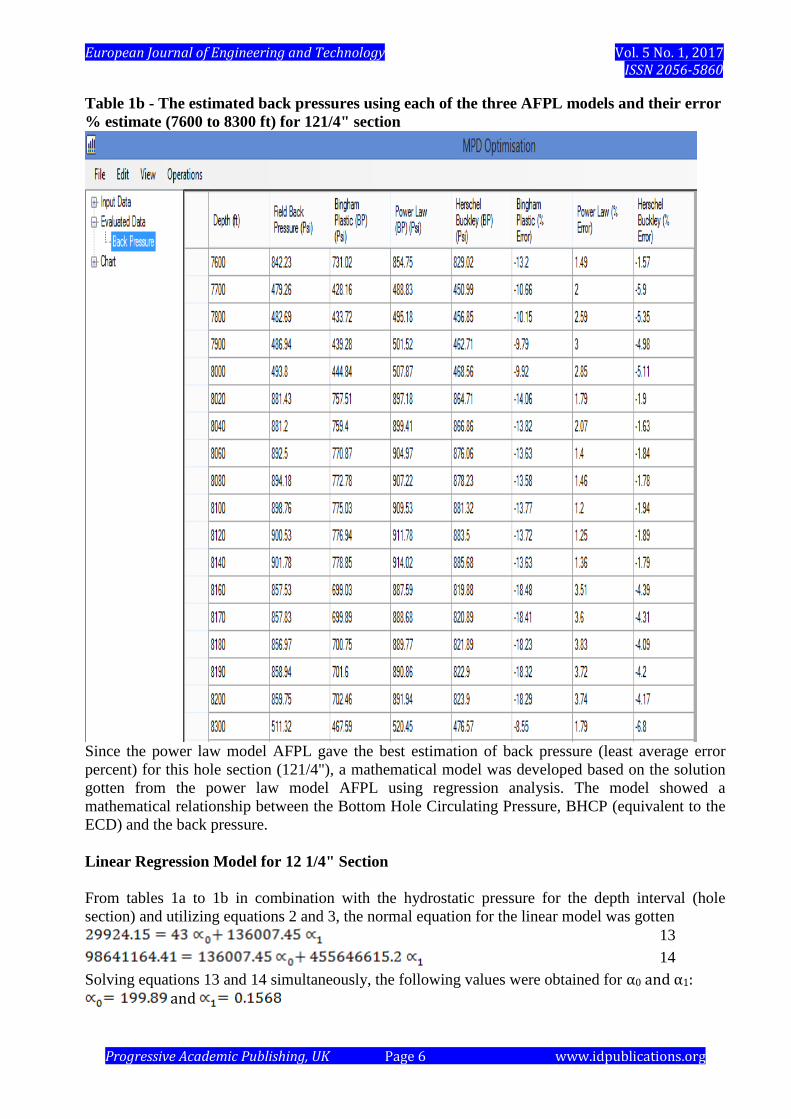
Table 1b - The estimated back pressures using each of the three AFPL models and their error
% estimate (7600 to 8300 ft) for 121/4" section
Since the power law model AFPL gave the best estimation of back pressure (least average error
percent) for this hole section (121/4"), a mathematical model was developed based on the solution
gotten from the power law model AFPL using regression analysis. The model showed a
mathematical relationship between the Bottom Hole Circulating Pressure, BHCP (equivalent to the
ECD) and the back pressure.
Linear Regression Model for 12 1/4" Section
From tables 1a to 1b in combination with the hydrostatic pressure for the depth interval (hole
section) and utilizing equations 2 and 3, the normal equation for the linear model was gotten
13
14
Solving equations 13 and 14 simultaneously, the following values were obtained for ⍺0 and ⍺1: and
European Journal of Engineering and Technology Vol. 5 No. 1, 2017 ISSN 2056-5860
Progressive Academic Publishing, UK Page 7 www.idpublications.org
Hence the Linear regression model is given as
Y = 199.89 + 0.1568x 15 Back pressure = 199.89 + 0.1568 BHCP 16 Equation 16 is the linear regression model for back pressure in terms of BHCP for this hole section.
Note: BHCP = AFPL + HP
Quadratic Regression Model for 12 1/4" Section
From tables 1a to 1b in combination with the hydrostatic pressure for the depth interval and
utilizing equations 5, 6 and 7, the quadratic model was gotten as shown below:
, and
Hence the quadratic regression model is given as:
17
18
Equations 18 is the quadratic regression model for back pressure in terms of BHCP for this hole
section.
Cubic Regression Model for 12 1/4" Section
From tables 1a to 1b in combination with the hydrostatic pressure for the depth interval and
utilizing equations 9, 10, 11 and 12, the cubic model was gotten as shown below:
, and
Hence the cubic regression model is given as shown below:
19
20
Equation 20 is the cubic model regression model for back pressure in terms of BHCP for this hole
section.

European Journal of Engineering and Technology Vol. 5 No. 1, 2017 ISSN 2056-5860
Progressive Academic Publishing, UK Page 8 www.idpublications.org
Table 2a - The estimated back pressures using each of the three AFPL models and their error
% estimate (8300 to 12500 ft) for 81/2" section

European Journal of Engineering and Technology Vol. 5 No. 1, 2017 ISSN 2056-5860
Progressive Academic Publishing, UK Page 9 www.idpublications.org
Table 2b - The estimated back pressures using each of the three AFPL models and their error
% estimate (12700 to 13500 ft) for 81/2" section
For this hole section, the Herschel Bulkley model AFPL performed best on the average. Hence the
estimated back pressure using the Herschel Bulkley model AFPL was the basis for the mathematical
model developed for this hole section. Just as for the 121/4" hole section, a mathematical model
was developed for this 81/2" hole section using regression analysis. The model gave a mathematical
relationship between the Bottom Hole Circulating Pressure, BHCP (which is like the ECD but in
Psi) and the back pressure.
Linear Regression Model for 8 1/2" Section
From tables 2a to 2b in combination with the hydrostatic pressure for this hole section and utilizing
equations 2 and 3, the normal equation for the linear model was gotten and shown below:
21
22

European Journal of Engineering and Technology Vol. 5 No. 1, 2017 ISSN 2056-5860
Progressive Academic Publishing, UK Page 10 www.idpublications.org
Solving equations 21 and 22 simultaneously, the values of ⍺0 and ⍺1 were obtained.
And
Hence the linear regression model is given as shown below:
23
24
Equation 24 is the linear regression model for back pressure in terms of the BHCP for this 8 1/2"
hole section.
Quadratic Regression Model for 8 1/2" Section
From tables 2a to 2b in combination with the hydrostatic pressure for this hole section and utilizing
equations 5,6 and 7, the quadratic model was gotten and it is shown below:
, and
Hence the quadratic model is given as shown below:
25
26
Equation 26 is the quadratic regression model for back pressure in terms of the BHCP for this 8
1/2" hole section.
Cubic Regression Model for 8 1/2" Section
From tables 2a to 2b in combination with the hydrostatic pressure for this hole section and the
normal equation (equations 9, 10,11 and 12), the cubic regression model was gotten and it is shown
below:
, , and
Hence, the cubic model is given as shown below;
27
28
Equation 28 is the cubic regression model for back pressure in terms of the BHCP for this 8 1/2"
hole section.
Model Validation Using Actual Field Data for the various Intervals
The developed regression models were validated with the actual field data. The various models
(linear, quadratic and cubic models) were used to estimate the back pressures, the estimated values
were plotted against the actual field back pressure, the correlation coefficient between the respective
regression models and the actual field data were estimated, the model with the highest correlation
coefficient (R2) value was taken as the best.
For the 12 1/4" Hole Section
From equations 16, 18 and 20 the back pressures were estimated for linear, quadratic and cubic
models respectively. (See estimated results in table 7 of the appendix)

European Journal of Engineering and Technology Vol. 5 No. 1, 2017 ISSN 2056-5860
Progressive Academic Publishing, UK Page 11 www.idpublications.org
Figure 1 - Plots of back pressure against the BHCP for the 121/4" section
The correlation coefficients for the results from the regression models are shown below with their
rank:
Table 3 - Rank of the regression models Models Correlation Coefficient Rank
Linear 0.7007 3rd
Quadratic 0.8058 1st
Cubic 0.7862 2nd
Hence the Quadratic model (equation 18) from the three regression models compared gave the best
approximation for back pressure for the 121/4" hole section. This means that the model gives
80.58% representation of the desirable data.
For the 8 1/2" hole section
From equations 24, 26 and 28 the back pressures were estimated for linear, quadratic and cubic
models respectively. (See estimated results in table 8 of the appendix)

European Journal of Engineering and Technology Vol. 5 No. 1, 2017 ISSN 2056-5860
Progressive Academic Publishing, UK Page 12 www.idpublications.org
Figure 2 - Plot of Back Pressure against BHCP for the 81/2" hole section
The correlation coefficients for the results from the regression models are shown below with their
rank:
Table 4 - Rank of the regression models Models Correlation Coefficient Rank
Linear 0.8907 3rd
Quadratic 0.9128 1st
Cubic 0.8962 2nd
The result showed that the Quadratic model (equation 26) from the three regression models
compared gave the best approximation for back pressure estimation for the 81/2" hole section. This
means that the model gives 91.28% representation of the desirable data.
CONCLUSIONS
The ability to precisely control the pressures in the wellbore will go a long way in helping us to
eradicate and minimize drilling problems such as; lost circulation, borehole instability, kick and
stuck pipe. Based on this study, it is concluded that an accurate estimation of the required back
pressure is very necessary for a successful MPD operation when using the CBHP technique. The
mathematical models developed for back pressure estimation based on the bottom hole circulating
pressure (ECD) is reliable and efficient. The quadratic model showed the best approximation for the
actual field back pressure for the two hole sections analyzed in this study. Hence with the ECD, the
required back pressure for a CBHP MPD operation can be confidently predicted using the quadratic
regression models developed in this study.
REFERENCES
Aadnoy, B., Cooper, I., Misca S., Mitchell, R.F., Payne, M.L. (2009): “Advanced Drilling and Well
Technology”
Demirdal, B., Cunha, J.C. (2007). "New Improvements on Managed Pressure Drilling", presented at
the Petroleum Society's 8th
Canadian International Petroleum Conference, Calgary, Alberta,
Canada, June 12-14, 2007.
Elieff, B.A.M. (2006) “Top Hole Drilling with Dual Gradient Technology to Control Shallow
Hazards”, M.Sc. Thesis, Texas A&M University, August 2006.
Fan, H., Wang, G., Peng, Q., Wang, Y. (2014). "Utility Hydraulic Calculation Model of Herschel
Bulkey Rheology Model for MPD Hydraulics", presented at the SPE Asia Pacific Oil & Gas
Conference and Exhibition held in Adelaide, Australia, 14-16 October 2014. SPE 171443
MS
Glen-Ole, K., Oyvind, N.S., Lars, I., and Ole, M.A "Simplified Hydraulics Model Used For a
Managed Pressure Drilling Control System", presented at the SPE/IADC Managed Pressure
Drilling and Underbalanced Operations Conference and Exhibition, Denver. SPE 143097.
Hannegan, D. (2006). “Case Studies – Offshore Managed Pressure Drilling”, presentation at the
2006 SPE Annual Technical Conference and Exhibition held in San Antonio, Texas,
U.S.A.,101855, 24–27 September.
Hannegan, D. (2010). “Drill thru the Limits-Concepts and Enabling Tools”, paper presented in
SPE/IADC Managed Pressure Drilling and Underbalanced Operations Conference and
Exhibition, Kuala Lumpur, Malaysia, 24-25 February 2010.
Hannegan, D. (2009). “Offshore Drilling Hazard Mitigation: Controlled Pressure Drilling Redefines
What Is Drillable”, Drilling Contractor Journal, January/February 2009, 84-89.
International Association of Drilling Contractors, “Improved Drilling Fluids Advances
Operations”,http://iadc.org/dcpi/dcjanfeb06/Jan06-AB01.pdf

European Journal of Engineering and Technology Vol. 5 No. 1, 2017 ISSN 2056-5860
Progressive Academic Publishing, UK Page 13 www.idpublications.org
Jan, E., and Hardy, S. (2014). "Back Pressure MPD in Extended Reach Wells-Limiting Factors For
the Ability to Achieve Accurate Pressure Control", presented at the SPE Bergen one day
Seminar Held in Grieghallen, Bergen, Norway, 2 April 2014. SPE 169211 MS.
Kinik, K., Gumus, F. and Osayande, N. (2015). "Automated Dynamic Well Control With Managed-
Pressure Drilling: A Case Study and Simulation Analysis", presented at the SPE/IADC
Managed Pressure Drilling & Underbalanced Operations Conference & Exhibition, Madrid,
Spain.
Malloy, K.P. (2007). “Managed Pressure Drilling- What is it anyway?” Journal of World Oil, PP
27-34.
Malloy, K.P., McDonald, P. (2008). “A Probabilistic Approach to Risk Assessment of Managed
Pressure Drilling in Offshore 191 Applications”, Joint Industry Project DEA 155,
Technology. Assessment and Research Study 582 Contract 0106CT39728
Medley, G.H., Reynolds, P.B.B. (2006). “Distinct Variations of Managed Pressure Drilling Exhibit
Application Potential”, World Oil Magazine Archive, Vol. 227, No. 3, PP 1-7.
Rehm, B., Schubert, J., Haghshenas, A., Paknejad, A.S., Hughes, J.(2008) “Managed Pressure
Drilling”, Gulf Drilling Series,Houston, Texas, PP 3,4,21-23,229-231,241-248.
Syltøy, S., Eide, S.E., Torvund, S., Berg, P.C., Larsen, T., Fjeldberg, H., Bjørkevoll, K.S.,
McCaskill, J., Prebensen, O.I., Low, E., (2008).“Multi-technical MPD Concept,
Comprehensive Planning Extend HPHT Targets on Kvitebjørn”, Journal of Drilling
Contractor, May/June 2008, 96-101.
APPENDIX
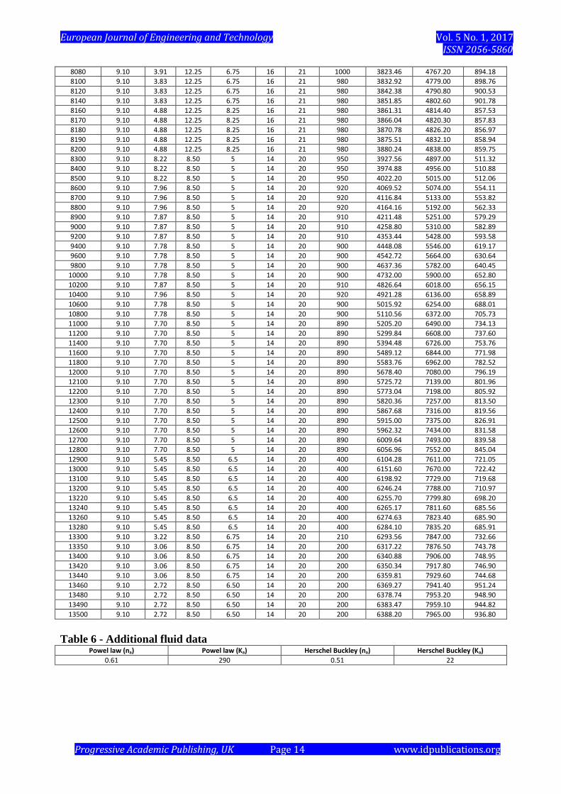
Table 5 - Drilling data from a Well X in West Africa
Depth, ft Densitypp
g V, ft/s
hole size, inch
O.D, inches
PV, Cp
YP, lb/100f
t2 Q,gpm HP, Psi PP, Psi
Back Pressure,
psi
3980 9.10 3.85 12.25 6.625 16 21 1000 1883.34 2348.20 443.32
4000 9.10 3.85 12.25 6.625 16 21 1000 1892.80 2360.00 444.49
4100 9.10 3.85 12.25 6.625 16 21 1000 1940.12 2419.00 454.55
4200 9.10 3.85 12.25 6.625 16 21 1000 1987.44 2478.00 465.55
4300 9.10 3.85 12.25 6.625 16 21 1000 2034.76 2537.00 476.33
4400 9.10 3.85 12.25 6.625 16 21 1000 2082.08 2596.00 487.80
4500 9.10 3.85 12.25 6.625 16 21 1000 2129.40 2655.00 498.97
4600 9.10 3.85 12.25 6.625 16 21 1000 2176.72 2714.00 510.16
4700 9.10 3.85 12.25 6.625 16 21 1000 2224.04 2773.00 521.11
4800 9.10 3.85 12.25 6.625 16 21 1000 2271.36 2832.00 532.53
4900 9.10 3.85 12.25 6.625 16 21 1000 2318.68 2891.00 543.44
5000 9.10 3.85 12.25 6.625 16 21 1000 2366.00 2950.00 554.68
5200 9.10 3.85 12.25 6.625 16 21 1000 2460.64 3068.00 577.44
5400 9.10 3.85 12.25 6.625 16 21 1000 2555.28 3186.00 600.18
5600 9.10 3.85 12.25 6.625 16 21 1000 2649.92 3304.00 621.61
5800 9.10 3.85 12.25 6.625 16 21 1000 2744.56 3422.00 643.69
6000 9.10 3.85 12.25 6.625 16 21 1000 2839.20 3540.00 665.93
6300 9.10 3.85 12.25 6.625 16 21 1000 2981.16 3717.00 699.72
6600 9.10 3.85 12.25 6.625 16 21 1000 3123.12 3894.00 731.12
6900 9.10 3.85 12.25 6.625 16 21 1000 3265.08 4071.00 764.47
7000 9.10 3.85 12.25 6.625 16 21 1000 3312.40 4130.00 775.71
7100 9.10 3.85 12.25 6.625 16 21 1000 3359.72 4189.00 787.17
7200 9.10 3.85 12.25 6.625 16 21 1000 3407.04 4248.00 798.07
7300 9.10 3.85 12.25 6.625 16 21 1000 3454.36 4307.00 809.08
7400 9.10 3.85 12.25 6.625 16 21 1000 3501.68 4366.00 820.11
7500 9.10 3.85 12.25 6.625 16 21 1000 3549.00 4425.00 831.00
7600 9.10 3.85 12.25 6.625 16 21 1000 3596.32 4484.00 842.23
7700 9.10 6.83 12.25 9.5 16 21 1000 3643.64 4543.00 479.26
7800 9.10 6.83 12.25 9.5 16 21 1000 3690.96 4602.00 482.69
7900 9.10 6.83 12.25 9.5 16 21 1000 3738.28 4661.00 486.94
8000 9.10 6.83 12.25 9.5 16 21 1000 3785.60 4720.00 493.80
8020 9.10 4.04 12.25 7 16 21 1000 3795.06 4731.80 881.43
8040 9.10 4.04 12.25 7 16 21 1000 3804.53 4743.60 881.20
8060 9.10 3.91 12.25 6.75 16 21 1000 3813.99 4755.40 892.50
European Journal of Engineering and Technology Vol. 5 No. 1, 2017 ISSN 2056-5860
Progressive Academic Publishing, UK Page 14 www.idpublications.org
8080 9.10 3.91 12.25 6.75 16 21 1000 3823.46 4767.20 894.18
8100 9.10 3.83 12.25 6.75 16 21 980 3832.92 4779.00 898.76
8120 9.10 3.83 12.25 6.75 16 21 980 3842.38 4790.80 900.53
8140 9.10 3.83 12.25 6.75 16 21 980 3851.85 4802.60 901.78
8160 9.10 4.88 12.25 8.25 16 21 980 3861.31 4814.40 857.53
8170 9.10 4.88 12.25 8.25 16 21 980 3866.04 4820.30 857.83
8180 9.10 4.88 12.25 8.25 16 21 980 3870.78 4826.20 856.97
8190 9.10 4.88 12.25 8.25 16 21 980 3875.51 4832.10 858.94
8200 9.10 4.88 12.25 8.25 16 21 980 3880.24 4838.00 859.75
8300 9.10 8.22 8.50 5 14 20 950 3927.56 4897.00 511.32
8400 9.10 8.22 8.50 5 14 20 950 3974.88 4956.00 510.88
8500 9.10 8.22 8.50 5 14 20 950 4022.20 5015.00 512.06
8600 9.10 7.96 8.50 5 14 20 920 4069.52 5074.00 554.11
8700 9.10 7.96 8.50 5 14 20 920 4116.84 5133.00 553.82
8800 9.10 7.96 8.50 5 14 20 920 4164.16 5192.00 562.33
8900 9.10 7.87 8.50 5 14 20 910 4211.48 5251.00 579.29
9000 9.10 7.87 8.50 5 14 20 910 4258.80 5310.00 582.89
9200 9.10 7.87 8.50 5 14 20 910 4353.44 5428.00 593.58
9400 9.10 7.78 8.50 5 14 20 900 4448.08 5546.00 619.17
9600 9.10 7.78 8.50 5 14 20 900 4542.72 5664.00 630.64
9800 9.10 7.78 8.50 5 14 20 900 4637.36 5782.00 640.45
10000 9.10 7.78 8.50 5 14 20 900 4732.00 5900.00 652.80
10200 9.10 7.87 8.50 5 14 20 910 4826.64 6018.00 656.15
10400 9.10 7.96 8.50 5 14 20 920 4921.28 6136.00 658.89
10600 9.10 7.78 8.50 5 14 20 900 5015.92 6254.00 688.01
10800 9.10 7.78 8.50 5 14 20 900 5110.56 6372.00 705.73
11000 9.10 7.70 8.50 5 14 20 890 5205.20 6490.00 734.13
11200 9.10 7.70 8.50 5 14 20 890 5299.84 6608.00 737.60
11400 9.10 7.70 8.50 5 14 20 890 5394.48 6726.00 753.76
11600 9.10 7.70 8.50 5 14 20 890 5489.12 6844.00 771.98
11800 9.10 7.70 8.50 5 14 20 890 5583.76 6962.00 782.52
12000 9.10 7.70 8.50 5 14 20 890 5678.40 7080.00 796.19
12100 9.10 7.70 8.50 5 14 20 890 5725.72 7139.00 801.96
12200 9.10 7.70 8.50 5 14 20 890 5773.04 7198.00 805.92
12300 9.10 7.70 8.50 5 14 20 890 5820.36 7257.00 813.50
12400 9.10 7.70 8.50 5 14 20 890 5867.68 7316.00 819.56
12500 9.10 7.70 8.50 5 14 20 890 5915.00 7375.00 826.91
12600 9.10 7.70 8.50 5 14 20 890 5962.32 7434.00 831.58
12700 9.10 7.70 8.50 5 14 20 890 6009.64 7493.00 839.58
12800 9.10 7.70 8.50 5 14 20 890 6056.96 7552.00 845.04
12900 9.10 5.45 8.50 6.5 14 20 400 6104.28 7611.00 721.05
13000 9.10 5.45 8.50 6.5 14 20 400 6151.60 7670.00 722.42
13100 9.10 5.45 8.50 6.5 14 20 400 6198.92 7729.00 719.68
13200 9.10 5.45 8.50 6.5 14 20 400 6246.24 7788.00 710.97
13220 9.10 5.45 8.50 6.5 14 20 400 6255.70 7799.80 698.20
13240 9.10 5.45 8.50 6.5 14 20 400 6265.17 7811.60 685.56
13260 9.10 5.45 8.50 6.5 14 20 400 6274.63 7823.40 685.90
13280 9.10 5.45 8.50 6.5 14 20 400 6284.10 7835.20 685.91
13300 9.10 3.22 8.50 6.75 14 20 210 6293.56 7847.00 732.66
13350 9.10 3.06 8.50 6.75 14 20 200 6317.22 7876.50 743.78
13400 9.10 3.06 8.50 6.75 14 20 200 6340.88 7906.00 748.95
13420 9.10 3.06 8.50 6.75 14 20 200 6350.34 7917.80 746.90
13440 9.10 3.06 8.50 6.75 14 20 200 6359.81 7929.60 744.68
13460 9.10 2.72 8.50 6.50 14 20 200 6369.27 7941.40 951.24
13480 9.10 2.72 8.50 6.50 14 20 200 6378.74 7953.20 948.90
13490 9.10 2.72 8.50 6.50 14 20 200 6383.47 7959.10 944.82
13500 9.10 2.72 8.50 6.50 14 20 200 6388.20 7965.00 936.80
Table 6 - Additional fluid data Powel law (na) Powel law (Ka) Herschel Buckley (na) Herschel Buckley (Ka)
0.61 290 0.51 22

European Journal of Engineering and Technology Vol. 5 No. 1, 2017 ISSN 2056-5860
Progressive Academic Publishing, UK Page 15 www.idpublications.org
Table 7 - Results from the regression models used in the 121/4" hole section BHCP, Psi Actual Back Pressure,
Psi
Linear Model Back
Pressure, Psi
Quadratic Model Back
Pressure, Psi
Cubic Model Back
Pressure, Psi
1900.58 447.62 497.90 372.11 352.86
1910.13 449.87 499.40 377.55 359.28
1957.88 461.12 506.89 404.27 390.62
2005.64 472.36 514.37 430.15 420.68
2053.39 483.61 521.86 455.21 449.49
2101.14 494.86 529.35 479.43 477.07
2148.90 506.10 536.84 502.83 503.42
2196.65 517.35 544.32 525.39 528.58
2244.40 528.60 551.81 547.13 552.55
2292.16 539.84 559.30 568.03 575.35
2339.91 551.09 566.79 588.10 597.01
2387.66 562.34 574.28 607.35 617.54
2483.17 584.83 589.25 643.35 655.26
2578.68 607.32 604.23 676.03 688.68
2674.18 629.82 619.20 705.39 717.92
2769.69 652.31 634.18 731.42 743.12
2865.20 674.80 649.15 754.14 764.44
3008.46 708.54 671.62 782.00 789.42
3151.72 742.28 694.08 802.38 806.42
3294.98 776.02 716.54 815.29 815.93
3342.73 787.27 724.03 817.94 817.51
3390.48 798.52 731.52 819.75 818.34
3438.24 809.76 739.01 820.73 818.41
3485.99 821.01 746.49 820.89 817.76
3533.74 832.26 753.98 820.21 816.40
3581.50 843.50 761.47 818.71 814.34
3629.25 854.75 768.96 816.37 811.61
4054.16 488.84 835.58 759.04 760.37
4106.81 495.19 843.84 747.35 751.00
4159.47 501.53 852.09 734.66 741.05
4212.12 507.88 860.35 720.97 730.53
3834.62 897.18 801.16 796.86 792.59
3844.19 899.41 802.66 795.58 791.43
3850.43 904.97 803.64 794.73 790.66
3859.98 907.22 805.14 793.39 789.46
3869.47 909.53 806.62 792.03 788.25
3879.02 911.78 808.12 790.63 787.01
3888.58 914.02 809.62 789.19 785.75
3926.81 887.59 815.61 783.12 780.46
3931.62 888.68 816.37 782.31 779.77
3936.43 889.77 817.12 781.50 779.07
3941.25 890.85 817.88 780.68 778.37
3946.06 891.94 818.63 779.85 777.67
Table 8 Results from the regression models used in the 81/2" hole section BHCP, Psi Actual Back Pressure,
Psi
Linear Model Back
Pressure, Psi
Quadratic Model Back
Pressure, Psi
Cubic Model Back
Pressure, Psi
4420.30 476.70 500.24 481.14 471.97
4473.55 482.45 507.88 491.32 484.42
4526.81 488.19 515.52 501.41 496.56
4551.90 522.10 519.12 506.13 502.17
4604.83 528.17 526.71 516.01 513.80
4657.76 534.24 534.30 525.79 525.14
4701.14 549.86 540.52 533.74 534.23
4753.96 556.04 548.09 543.33 545.05
4859.60 568.40 563.24 562.22 565.91
4955.24 590.76 576.96 578.99 583.95
5060.67 603.33 592.07 597.12 602.95
5166.10 615.90 607.19 614.86 621.08
5271.53 628.47 622.31 632.21 638.42
5387.82 630.18 638.99 650.91 656.69
5504.63 631.37 655.74 669.23 674.23
5587.82 666.18 667.67 681.98 686.26
5693.26 678.74 682.79 697.81 701.02

European Journal of Engineering and Technology Vol. 5 No. 1, 2017 ISSN 2056-5860
Progressive Academic Publishing, UK Page 16 www.idpublications.org
5787.08 702.92 696.24 711.57 713.75
5892.30 715.70 711.33 726.64 727.62
5997.52 728.48 726.42 741.33 741.12
6102.74 741.26 741.51 755.63 754.31
6207.96 754.04 756.60 769.56 767.26
6313.18 766.82 771.68 783.10 780.03
6365.79 773.21 779.23 789.73 786.37
6418.40 779.60 786.77 796.26 792.68
6471.01 785.99 794.32 802.70 798.98
6523.62 792.38 801.86 809.04 805.27
6576.23 798.77 809.41 815.29 811.57
6628.83 805.17 816.95 821.44 817.87
6681.44 811.56 824.49 827.50 824.19
6734.05 817.95 832.04 833.46 830.54
6874.99 736.01 852.25 848.96 847.72
6928.29 741.71 859.89 854.64 854.31
6981.58 747.42 867.53 860.22 860.96
7034.88 753.12 875.18 865.71 867.68
7045.54 754.26 876.71 866.80 869.03
7056.20 755.40 878.23 867.88 870.39
7066.85 756.55 879.76 868.95 871.75
7077.51 757.69 881.29 870.03 873.11
6973.86 873.14 866.43 859.42 859.99
6976.23 900.27 866.77 859.67 860.28
7002.36 903.64 870.51 862.37 863.57
7012.81 904.99 872.01 863.45 864.88
7023.26 906.34 873.51 864.52 866.21
6854.13 1087.27 849.26 846.71 845.15
6864.32 1088.88 850.72 847.81 846.40
6869.41 1089.69 851.45 848.36 847.03
6874.50 1090.50 852.18 848.90 847.66