A Fuzzy E.O.Q Model With Unit Production Cost, Time ... · YYYYYYYYYYYYYYYYY support Figure 2: Trapezoidal fuzzy number of 𝐴̃ with α-cuts. Aα is a non-empty bounded closed interval

* Corresponding Author. Email address: [email protected]; Tel: +91 9153222799 1

A Fuzzy E.O.Q Model With Unit Production Cost, Time Depended

Holding Cost, With-Out Shortages Under A Space Constraint: A

Fuzzy Geometric Programing (FGP) Approach

Sahidul Islam1, Wasim Akram Mandal2*

(1) Department of mathematics, University of kalyani, kalyani, W.B, India

(2) Beldanga D.H.Sr.Madrasah, Beldanga-742189, Murshidabad, WB, India

Copyright 2017 © Sahidul Islam and Wasim Akram Mandal. This is an open access article distributed under the

Creative Commons Attribution License, which permits unrestricted use, distribution, and reproduction in any

medium, provided the original work is properly cited.

Abstract

In this paper, an Economic Order quantity (E.O.Q) model with unit production cost, time depended

holding cost, with-out shortages is formulated and solved. In most real world situation, the objective

and constraint function of the decision makers are uncertainty in nature so the coefficients, indices the

objective function and constraint goals are imposed here in fuzzy environment The problem is then solved

using both Fuzzy Max-Min Geometric-Programming technique and Fuzzy parametric Geometric-

Programming. Sensitivity analysis is also presented here.

Keywords: E.O.Q model, Fuzzy set, Max-Min operator, Geometric Programming, Parametric Geometric

Programming Technique.

2010 Mathematics Subject Classification: 90B05, 90C70.

1 Introduction

An inventory deals with decision that minimize the cost function or maximize the profit function. For

this purpose the task is to construct a suitable mathematical model of the real life Inventory system, such a

mathematical model is based on various assumption and approximation.

Production and hosting by ISPACS GmbH.

Oxford Journal of Intelligent Decision and Data Science 2017 No. 1 (2017) 1-14

Available online at www.ispacs.com/ojids

Volume 2017, Issue 1, Year 2017 Article ID ojids-00009, 14 Pages

doi:10.5899/2017/ojids-00009

Research Article

Oxford Journal of Intelligent Decision and Data Science 2017 No. 1 (2017) 1-14 2

http://www.ispacs.com/journals/ojids/2017/ojids-00009/

International Scientific Publications and Consulting Services

In ordinary inventory model it considers all parameter like set-up cost, carrying cost, interest cost,

shortages etc as a fixed. But in real life situation it will have some little fluctuations. So consideration of

fuzzy variables is more realistic.

Since late 1960’s, Geometric Programming (GP) used in various field (like OR, Engineering science etc.).

Geometric Programming (GP) is one of the effective methods to solve a particular type of Non linear

programming (NLP) problem. The theory of Geometric Programming (GP) first emerged in 1961 by

Duffin and Zener and it further developed by Duffin. Duffin R J, Peterson E L, Zener C M studied

Geometric Programming-Theory and Application. Friedman (1978) developed continuous time inventory

model with time varying demand. Ritchie (1984) studied in inventory model with linear increasing

demand. Goswami, Chaudhuri (1991) presented an inventory model with shortage. Gen et. Al. (1997)

proposed classical inventory model with Triangular fuzzy number. Yao and Lee (1998) presented an

economic production quantity (EPQ) model in the fuzzy sense. Sujit Kumar De, P.K.Kundu and

A.Goswami (2003) discussed an economic production quantity (EPQ) inventory model involving fuzzy

demand rate. J.K.Syde and L.A.Aziz (2007) applied sign distance method to fuzzy inventory model

without shortages. D.Datta and Pravin Kumar published several papers of fuzzy inventory with or without

shortage. S. Islam, T.K. Roy (2006) presented a fuzzy EPQ model with flexibility and reliability

consideration and demand depended unit Production cost under a space constraint

S. Islam, T.K. Roy (2010), studied Multi-Objective Geometric-Programming Problem and its Application.

A.M Kotb, Halaa, Fergancy (2011) presented Multi-item EOQ model with both demand-depended unit

cost and varying Lead time via Geometric Programming approach. Samir Dey and Tapan Kumar Roy

(2015) proposed Optimum shape design of structural model with imprecise coefficient by parametric

geometric programming.

In this paper we consider crisp inventory model, there after it transformed to fuzzy inventory mode and

developed by geometric programming approach. First we solved the model by Fuzzy Max-Min Geometric-

Programming technique and then it solved by Fuzzy parametric Geometric -Programming technique. At

last it made an example and solved it by both technique.

2 Mathematical Model

An Inventory model is developed under the following notations and assumptions:

2.1. Notations

I(t):Inventory level at any time, t≥0.

D: Demand per unit time, which is constant.

T: Cycle of length of the given inventory.

S: Set-up cost per unit time.

H: Holding cost per item per unit time, which is time depended.

P: Unit demand and set-up cost dependent production cost.

q: Production quantity per batch.

f(D,S): Unit production cost per cycle.

TAC(D,S,q):Total average cost per unit time.

w0: Space area per unit quantity.

W: Total storage space area of the inventory.

2.2. Assumptions

a) The inventory system involves only one item.

b) The replenishment occurs instantaneously at infinite rate.

c) The lead time is negligible.




d) Demand rate is constant.

e) The unit production cost is continuous function of demand and Set-up cost and take the following

form:

p= θ𝐷−𝑥𝑆−1, θ,x∈ ℝ (>0).

f) Holding cost time depended as at.

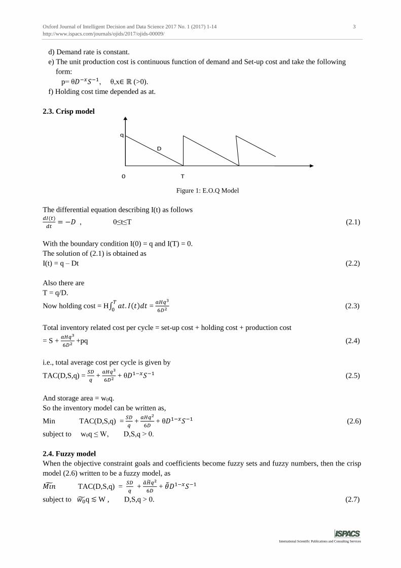
2.3. Crisp model

q

D

0 T

Figure 1: E.O.Q Model

The differential equation describing I(t) as follows 𝑑𝐼(𝑡)

𝑑𝑡= −𝐷 , 0≤t≤T (2.1)

With the boundary condition I(0) = q and I(T) = 0.

The solution of (2.1) is obtained as

I(t) = q – Dt (2.2)

Also there are

T = q/D.

Now holding cost = H∫ 𝑎𝑡. 𝐼(𝑡)𝑑𝑡𝑇

0 =

𝑎𝐻𝑞3

6𝐷2 (2.3)

Total inventory related cost per cycle = set-up cost + holding cost + production cost

= S + 𝑎𝐻𝑞3

6𝐷2 +pq (2.4)

i.e., total average cost per cycle is given by

TAC(D,S,q) = 𝑆𝐷

𝑞 +

𝑎𝐻𝑞3

6𝐷2 + θ𝐷1−𝑥𝑆−1 (2.5)

And storage area = w0q.

So the inventory model can be written as,

Min TAC(D,S,q) = 𝑆𝐷

𝑞 +

𝑎𝐻𝑞2

6𝐷 + θ𝐷1−𝑥𝑆−1 (2.6)

subject to w0q ≤ W, D,S,q > 0.

2.4. Fuzzy model

When the objective constraint goals and coefficients become fuzzy sets and fuzzy numbers, then the crisp

model (2.6) written to be a fuzzy model, as

𝑀𝑖�� TAC(D,S,q) = 𝑆𝐷

𝑞 +

��𝑞2

6𝐷 + ��𝐷1−𝑥𝑆−1

subject to 𝑤0q ≲ W , D,S,q > 0. (2.7)




3 Some basic concept & definition

3.1. Pre-requisite mathematics

Fuzzy sets first introduced by Zadeh [18] in 1965 as a mathematical way of representing vagueness in

every life.

Definition 3.1. A fuzzy set �� on the given universal set X is a set of order pairs, ��={(x,𝜇��(x): xϵX} where

𝜇�� (x)→[0,1] is called a membership function.

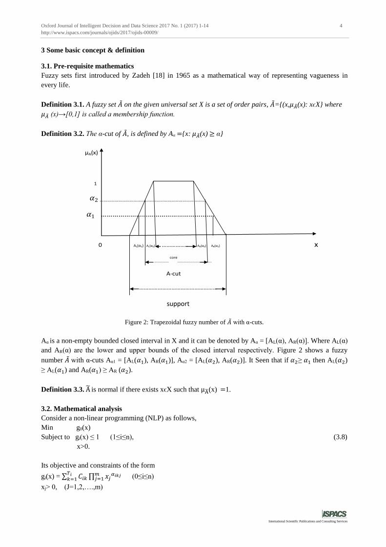
Definition 3.2. The α-cut of ��, is defined by Aα ={x: 𝜇��(x) ≥ α}

μA(x)

1

𝛼2 …………………………………………………………………………

𝛼1 ………………………………………………….

0 AL(α1) AL(α2) …………….. AR(α2) AR(α1) x

…………… core

……………………………..

Α-cut

……………………………………………

support

Figure 2: Trapezoidal fuzzy number of �� with α-cuts.

Aα is a non-empty bounded closed interval in X and it can be denoted by Aα = [AL(α), AR(α)]. Where AL(α)

and AR(α) are the lower and upper bounds of the closed interval respectively. Figure 2 shows a fuzzy

number �� with α-cuts Aα1 = [AL(𝛼1), AR(𝛼1)], Aα2 = [AL(𝛼2), AR(𝛼2)]. It Seen that if 𝛼2≥ 𝛼1 then AL(𝛼2)

≥ AL(𝛼1) and AR(𝛼1) ≥ AR (𝛼2).

Definition 3.3. A is normal if there exists xϵX such that μA(x) =1.

3.2. Mathematical analysis

Consider a non-linear programming (NLP) as follows,

Min g0(x)

Subject to gi(x) ≤ 1 (1≤i≤n), (3.8)

x>0.

Its objective and constraints of the form

gi(x) = ∑ 𝐶𝑖𝑘𝑇𝑖𝑘=1 ∏ 𝑥𝑗

𝛼𝑖𝑘𝑗𝑚𝑗=1 (0≤i≤n)

xj> 0, (J=1,2,….,m)




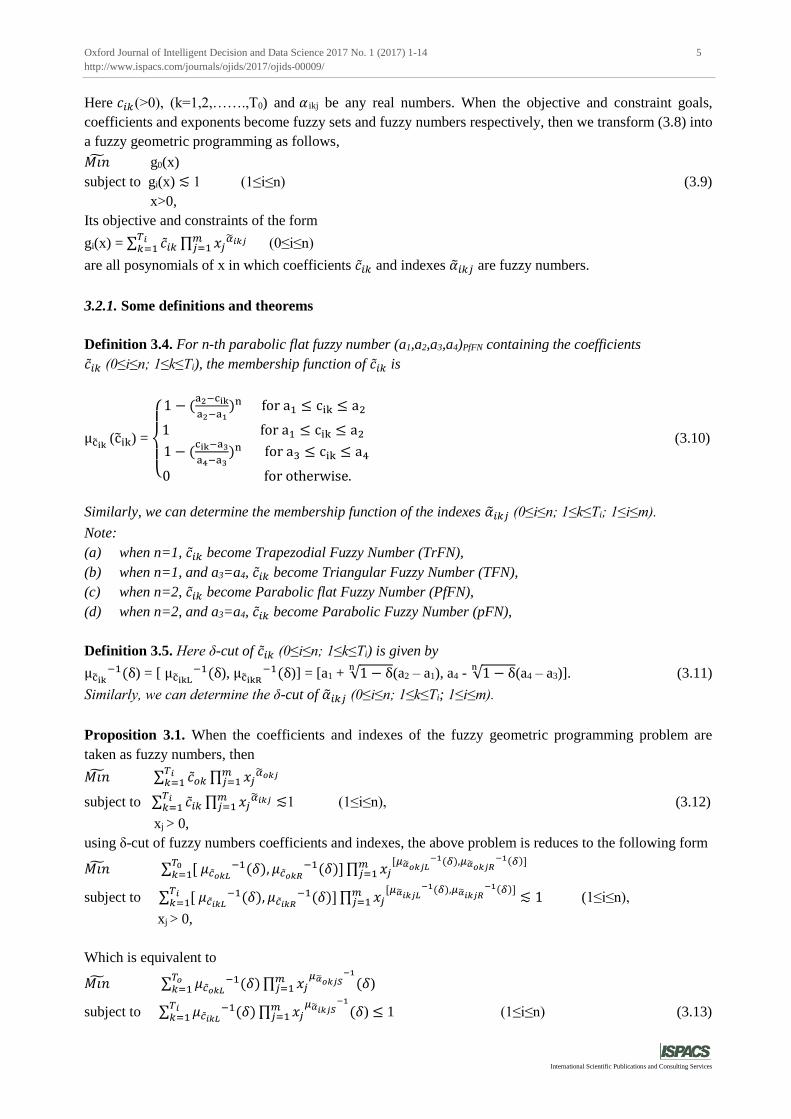
Here 𝑐𝑖𝑘(>0), (k=1,2,…….,T0) and 𝛼 ikj be any real numbers. When the objective and constraint goals,

coefficients and exponents become fuzzy sets and fuzzy numbers respectively, then we transform (3.8) into

a fuzzy geometric programming as follows,

𝑀𝑖�� g0(x)

subject to gi(x) ≲ 1 (1≤i≤n) (3.9)

x>0,

Its objective and constraints of the form

gi(x) = ∑ ��𝑖𝑘𝑇𝑖𝑘=1 ∏ 𝑥𝑗

��𝑖𝑘𝑗𝑚𝑗=1 (0≤i≤n)

are all posynomials of x in which coefficients ��𝑖𝑘 and indexes ��𝑖𝑘𝑗 are fuzzy numbers.

3.2.1. Some definitions and theorems

Definition 3.4. For n-th parabolic flat fuzzy number (a1,a2,a3,a4)PfFN containing the coefficients

��𝑖𝑘 (0≤i≤n; 1≤k≤Ti), the membership function of ��𝑖𝑘 is

μcik (cik) =

{

1 − (

a2−cik

a2−a1)n for a1 ≤ cik ≤ a2

1 for a1 ≤ cik ≤ a2

1 − (cik−a3

a4−a3)n for a3 ≤ cik ≤ a4

0 for otherwise.

(3.10)

Similarly, we can determine the membership function of the indexes ��𝑖𝑘𝑗 (0≤i≤n; 1≤k≤Ti; 1≤i≤m).

Note:

(a) when n=1, ��𝑖𝑘 become Trapezodial Fuzzy Number (TrFN),

(b) when n=1, and a3=a4, ��𝑖𝑘 become Triangular Fuzzy Number (TFN),

(c) when n=2, ��𝑖𝑘 become Parabolic flat Fuzzy Number (PfFN),

(d) when n=2, and a3=a4, ��𝑖𝑘 become Parabolic Fuzzy Number (pFN),

Definition 3.5. Here δ-cut of ��𝑖𝑘 (0≤i≤n; 1≤k≤Ti) is given by

μcik−1(δ) = [ μcikL

−1(δ), μcikR−1(δ)] = [a1 + √1 − δ

n(a2 – a1), a4 - √1 − δ

n(a4 – a3)]. (3.11)

Similarly, we can determine the δ-cut of ��𝑖𝑘𝑗 (0≤i≤n; 1≤k≤Ti; 1≤i≤m).

Proposition 3.1. When the coefficients and indexes of the fuzzy geometric programming problem are

taken as fuzzy numbers, then

𝑀𝑖�� ∑ ��𝑜𝑘𝑇𝑖𝑘=1 ∏ 𝑥𝑗

��𝑜𝑘𝑗𝑚𝑗=1

subject to ∑ ��𝑖𝑘𝑇𝑖𝑘=1 ∏ 𝑥𝑗

��𝑖𝑘𝑗𝑚𝑗=1 ≲1 (1≤i≤n), (3.12)

xj > 0,

using δ-cut of fuzzy numbers coefficients and indexes, the above problem is reduces to the following form

𝑀𝑖�� ∑ [ 𝜇𝑐𝑜𝑘𝐿−1(𝛿), 𝜇𝑐𝑜𝑘𝑅

−1(𝛿)]𝑇0𝑘=1 ∏ 𝑥𝑗

[𝜇��𝑜𝑘𝑗𝐿−1(𝛿),𝜇��𝑜𝑘𝑗𝑅

−1(𝛿)]𝑚𝑗=1

subject to ∑ [ 𝜇𝑐𝑖𝑘𝐿−1(𝛿), 𝜇𝑐𝑖𝑘𝑅

−1(𝛿)]𝑇𝑖𝑘=1 ∏ 𝑥𝑗

[𝜇��𝑖𝑘𝑗𝐿−1(𝛿),𝜇��𝑖𝑘𝑗𝑅

−1(𝛿)]𝑚𝑗=1 ≲ 1 (1≤i≤n),

xj > 0,

Which is equivalent to

𝑀𝑖�� ∑ 𝜇𝑐𝑜𝑘𝐿−1(𝛿)

𝑇𝑜𝑘=1 ∏ 𝑥𝑗

𝜇��𝑜𝑘𝑗𝑆−1

(𝛿𝑚𝑗=1 )

subject to ∑ 𝜇𝑐𝑖𝑘𝐿−1(𝛿)

𝑇𝑖𝑘=1 ∏ 𝑥𝑗

𝜇��𝑖𝑘𝑗𝑆−1

(𝛿𝑚𝑗=1 ) ≤ 1 (1≤i≤n) (3.13)




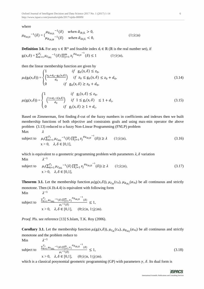
where

𝜇��𝑖𝑘𝑗𝑆−1(𝛿) = {

𝜇��𝑖𝑘𝑗𝐿−1(𝛿) 𝑤ℎ𝑒𝑛 ��𝑖𝑘𝑗𝐿 > 0,

𝜇��𝑖𝑘𝑗𝑅−1(𝛿) 𝑤ℎ𝑒𝑛 ��𝑖𝑘𝑗𝐿 < 0,

(1≤i≤n)

Definition 3.6. For any x ∈ ℝm and feasible index di ∈ ℝ (ℝ is the real number set), if

gi(x,𝛿) = ∑ 𝜇𝑐𝑖𝑘𝐿−1(𝛿)



(𝛿𝑚𝑗=1 ) ≤ 1 (1≤i≤n),

then the linear membership function are given by

𝜇0(g0(x,𝛿)) = {

1 𝑖𝑓 g0(x, 𝛿) ≤ 𝑧0,

(𝑧0+𝑑0−g0(x,𝛿)

𝑑0) 𝑖𝑓 𝑧0 ≤ g0(x, 𝛿)

0 𝑖𝑓 g0(x, 𝛿) ≥ 𝑧0 + 𝑑0,

≤ 𝑧0 + 𝑑0, (3.14)

𝜇i(gi(x,𝛿)) = {

1 𝑖𝑓 gi(x, 𝛿) ≤ 𝑧0,

(1+𝑑𝑖−i(x,𝛿)

𝑑0) 𝑖𝑓 1 ≤ gi(x, 𝛿)

0 𝑖𝑓 gi(x, 𝛿) ≥ 1 + 𝑑𝑖,

≤ 1 + 𝑑𝑖 , (3.15)

Based on Zimmerman, first finding 𝛿-cut of the fuzzy numbers in coefficients and indexes then we built

membership functions of both objective and constraints goals and using max-min operator the above

problem (3.13) reduced to a fuzzy Non-Linear Programming (FNLP) problem

Max 𝜆

subject to 𝜇𝑖(∑ 𝜇𝑐𝑖𝑘𝐿−1(𝛿)



𝑚𝑗=1 (𝛿)) ≥ 𝜆 (1≤i≤n), (3.16)

x > 0, 𝜆, 𝛿 ∈ [0,1],

which is equivalent to a geometric programming problem with parameters 𝜆, 𝛿 variation

Min 𝜆−1

subject to 𝜇𝑖(∑ 𝜇𝑐𝑖𝑘𝐿−1(𝛿)



𝑚𝑗=1 (𝛿)) ≥ 𝜆 (1≤i≤n), (3.17)

x > 0, 𝜆, 𝛿 ∈ [0,1],

Theorem 3.1. Let the membership function 𝜇i(gi(x,𝛿)), 𝜇𝑐𝑖𝑘(cik), 𝜇��𝑖𝑘𝑗(𝛼ikj) be all continuous and strictly

monotone. Then (4.1b.4.4) is equivalent with following form

Min 𝜆−1

subject to ∑ 𝜇��𝑖𝑘𝐿

−1(𝛿)𝑇𝑖𝑘=1

∏ 𝑥𝑗𝜇��𝑖𝑘𝑗𝑆

−1

(𝛿)𝑚𝑗=1

𝜇𝑖−1(𝛿)

≤ 1,

x > 0, 𝜆, 𝛿 ∈ [0,1], (0≤i≤n, 1≤j≤m).

Proof. Pls. see reference [13] S.Islam, T.K. Roy (2006).

Corollary 3.1. Let the membership function 𝜇i(gi(x,𝛿)), 𝜇𝑐𝑖𝑘(cik), 𝜇��𝑖𝑘𝑗(𝛼ikj) be all continuous and strictly

monotone and the problem reduce to

Min 𝜆−1

subject to ∑ 𝜇��𝑖𝑘𝐿

−1(𝛿)𝑇𝑖𝑘=1

∏ 𝑥𝑗𝜇��𝑖𝑘𝑗𝑆

−1

(𝛿)𝑚𝑗=1

𝜇𝑖−1(𝛿)

≤ 1, (3.18)

x > 0, 𝜆, 𝛿 ∈ [0,1], (0≤i≤n, 1≤j≤m).

which is a classical posynomial geometric programming (GP) with parameters 𝛾, 𝛿. Its dual form is




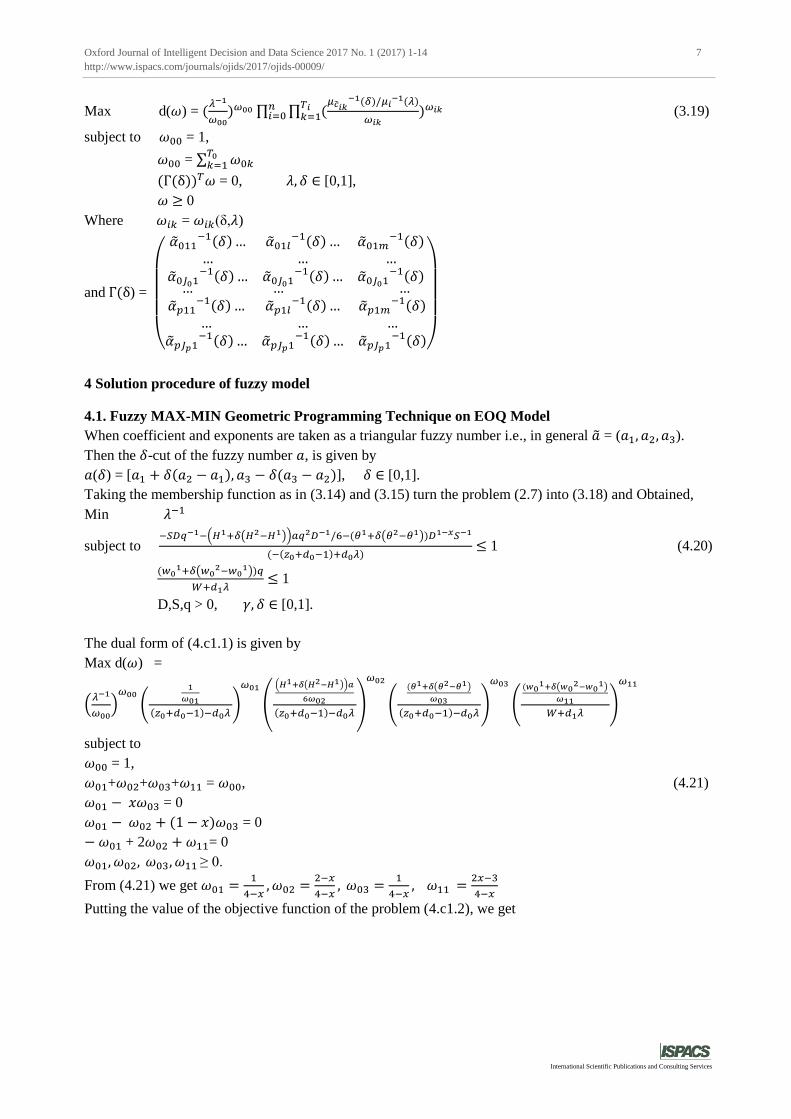
Max d(𝜔) = (𝜆−1

𝜔00)𝜔00 ∏ ∏ (

𝜇��𝑖𝑘−1(𝛿)/𝜇𝑖

−1(𝜆)

𝜔𝑖𝑘)𝜔𝑖𝑘

𝑇𝑖𝑘=1

𝑛𝑖=0 (3.19)

subject to 𝜔00 = 1,

𝜔00 = ∑ 𝜔0𝑘𝑇0𝑘=1

(Γ(δ))𝑇𝜔 = 0, 𝜆, 𝛿 ∈ [0,1],

𝜔 ≥ 0

Where 𝜔𝑖𝑘 = 𝜔𝑖𝑘(δ,𝜆)

and Γ(δ) =

(

��011−1(𝛿)… ��01𝑙

−1(𝛿)… ��01𝑚−1(𝛿)

… … …��0𝐽01

−1(𝛿)… ��0𝐽01−1(𝛿)… ��0𝐽01

−1(𝛿)… … …

��𝑝11−1(𝛿)… ��𝑝1𝑙

−1(𝛿)… ��𝑝1𝑚−1(𝛿)

… … …��𝑝𝐽𝑝1

−1(𝛿)… ��𝑝𝐽𝑝1−1(𝛿)… ��𝑝𝐽𝑝1

−1(𝛿))

4 Solution procedure of fuzzy model

4.1. Fuzzy MAX-MIN Geometric Programming Technique on EOQ Model

When coefficient and exponents are taken as a triangular fuzzy number i.e., in general �� = (𝑎1, 𝑎2, 𝑎3).

Then the 𝛿-cut of the fuzzy number 𝑎, is given by

𝑎(𝛿) = [𝑎1 + 𝛿(𝑎2 − 𝑎1), 𝑎3 − 𝛿(𝑎3 − 𝑎2)], 𝛿 ∈ [0,1].

Taking the membership function as in (3.14) and (3.15) turn the problem (2.7) into (3.18) and Obtained,

Min 𝜆−1

subject to −𝑆𝐷𝑞−1−(𝐻1+𝛿(𝐻2−𝐻1))𝑎𝑞2𝐷−1/6−(𝜃1+𝛿(𝜃2−𝜃1))𝐷1−𝑥𝑆−1

(−(𝑧0+𝑑0−1)+𝑑0𝜆) ≤ 1 (4.20)

(𝑤0

1+𝛿(𝑤02−𝑤0

1))𝑞

𝑊+𝑑1𝜆 ≤ 1

D,S,q > 0, 𝛾, 𝛿 ∈ [0,1].

The dual form of (4.c1.1) is given by

Max d(𝜔) =

(𝜆−1

𝜔00)𝜔00

(

1

𝜔01

(𝑧0+𝑑0−1)−𝑑0𝜆)

𝜔01

(

(𝐻1+𝛿(𝐻2−𝐻1))𝑎

6𝜔02

(𝑧0+𝑑0−1)−𝑑0𝜆)

𝜔02

(

(𝜃1+𝛿(𝜃2−𝜃1)

𝜔03

(𝑧0+𝑑0−1)−𝑑0𝜆)

𝜔03

(

(𝑤01+𝛿(𝑤0

2−𝑤01)

𝜔11

𝑊+𝑑1𝜆)

𝜔11

subject to

𝜔00 = 1,

𝜔01+𝜔02+𝜔03+𝜔11 = 𝜔00, (4.21)

𝜔01 − 𝑥𝜔03 = 0

𝜔01 − 𝜔02 + (1 − 𝑥)𝜔03 = 0

− 𝜔01 + 2𝜔02 +𝜔11= 0

𝜔01, 𝜔02, 𝜔03, 𝜔11 ≥ 0.

From (4.21) we get 𝜔01 =1

4−𝑥, 𝜔02 =

2−𝑥

4−𝑥, 𝜔03 =

1

4−𝑥, 𝜔11 =

2𝑥−3

4−𝑥

Putting the value of the objective function of the problem (4.c1.2), we get




d(𝜔) = 𝜆−1 (4−𝑥

(𝑧0+𝑑0−1)−𝑑0𝜆)

1

4−𝑥(

(𝐻1+𝛿(𝐻2−𝐻1))𝑎(4−𝑥)

6(2−𝑥)

(𝑧0+𝑑0−1)−𝑑0𝜆)

2−𝑥

4−𝑥

× ((𝜃1+𝛿(𝜃2−𝜃1)(4−𝑥)

(𝑧0+𝑑0−1)−𝑑0𝜆)

1

4−𝑥((𝑤0

1+𝛿(𝑤02−𝑤0

1)(4−𝑥)/(2𝑥−3)

𝑊+𝑑1𝜆)

2𝑥−3

4−𝑥 (2𝑥−3

4−𝑥)2𝑥−3

4−𝑥

We can obtained 𝜆 by the aid of d(𝜔) = 𝜆−1. Then the above equation is reduces to the following form

(4−𝑥

(𝑧0+𝑑0−1)−𝑑0𝜆)

1

4−𝑥(

(𝐻1+𝛿(𝐻2−𝐻1))𝑎(4−𝑥)

6(2−𝑥)

(𝑧0+𝑑0−1)−𝑑0𝜆)

2−𝑥

4−𝑥

× ((𝜃1+𝛿(𝜃2−𝜃1)(4−𝑥)

(𝑧0+𝑑0−1)−𝑑0𝜆)

1

4−𝑥((𝑤0

1+𝛿(𝑤02−𝑤0

1)(4−𝑥)/(2𝑥−3)

𝑊+𝑑1𝜆)

2𝑥−3

4−𝑥 (2𝑥−3

4−𝑥)2𝑥−3

4−𝑥 =1 (4.22)

Solving the above equation of 𝛾 for given 𝛿 ∈ [0,1] by Newton-Raphson method, we obtain the value of

𝜆∗. Putting the value of 𝜆∗, we obtained the values of the dual objective function.

Again from the between primal-dual relation, we get

−𝑆𝐷𝑞−1

(−(𝑧0+𝑑0−1)+𝑑0𝜆∗)

= 𝜔01

∗

𝜔00∗ =

1

4−𝑥,

−(𝐻1+𝛿(𝐻2−𝐻1))𝑎𝑞2𝐷−1/6

(−(𝑧0+𝑑0−1)+𝑑0𝜆∗)

= 𝜔02

∗

𝜔00∗ =

2−𝑥

4−𝑥,

−(𝜃1+𝛿(𝜃2−𝜃1))𝐷1−𝑥𝑆−1

(−(𝑧0+𝑑0−1)+𝑑0𝜆∗)

= 𝜔03

∗

𝜔00∗ =

1

4−𝑥,

(𝑤01+𝛿(𝑤0

2−𝑤01))𝑞

𝑊+𝑑1𝜆∗ =

𝜔11∗

𝜔11∗ =1. (4.23)

Solving (4.23) we have

S* =6𝜔1

⋆𝜔2⋆((𝑧0+𝑑0−1)−𝑑0𝜆

∗)2

𝑎(𝐻1+𝛿(𝐻2−𝐻1)),

D* = 𝑎(𝐻1+𝛿(𝐻2−𝐻1))𝑞2

6𝜔2∗((𝑧0+𝑑0−1)−𝑑0𝜆

∗),

q* = 𝑊+𝑑1𝜆

∗

(𝑤01+𝛿(𝑤0

2−𝑤01)) .

4.2. Fuzzy Parametric Geometric Programming Technique on EOQ Model

Taking �� = 𝐻1 + 𝛿(𝐻2 −𝐻1), �� =𝜃1 + 𝛿(𝜃2 − 𝜃1) , 𝑤0 = 𝑤01 + 𝛿(𝑤0

2 −𝑤01) , 𝑎𝑛𝑑 �� =𝑊1 +

𝛿(𝑊2 −𝑊1) where α∈ [0, 1] in (2.7). The model takes the reduces form as follows


𝑞 +

𝑎(𝐻1+𝛿(𝐻2−𝐻1))𝑞2

6𝐷 + (𝜃1 + 𝛿(𝜃2 − 𝜃1)))𝐷1−𝑥 𝑆−1 (4.24)

subject to (𝑤01 + 𝛿(𝑤0

2 −𝑤01)) q ≤ (𝑊1 + 𝛿(𝑊2 −𝑊1)) , D,S,q > 0.

Applying geometric programming GP technique the dual programming of the problem (4.24) is

Max 𝑑(𝜔) = (1

𝜔1) 𝜔1(

𝑎(𝐻1+𝛿(𝐻2−𝐻1))

6𝜔2)𝜔2(

𝜃1+𝛿(𝜃2−𝜃1)

𝜔3)𝜔3(

𝑤01+𝛿(𝑤0

2−𝑤01)

(𝑊1+𝛿(𝑊2−𝑊1)))𝜔01𝜔01

𝜔01

subject to 𝜔1 +𝜔2 +𝜔3 = 1,

𝜔1 − 𝜔3 = 0,

𝜔1 − 𝜔2 + (1-x)𝜔3= 0,

− 𝜔1 + 2𝜔2 +𝜔01= 0,

𝜔1, 𝜔2, 𝜔3, 𝜔01 ≥ 0.




i.e., we get 𝜔1 =1

4−𝑥, 𝜔2 =

2−𝑥

4−𝑥, 𝜔3 =

1

4−𝑥, 𝑎𝑛𝑑 𝜔01 =

2𝑥−3

4−𝑥.

Putting the values in (4.24) we get the optimal solution of dual problem. The values of D, S, q is obtained

by using the primal dual relation as follows;

From the primal dual relation we have, 𝑆𝐷

𝑞 = 𝜔1

⋆ × 𝑑∗(𝜔),

𝑎(𝐻1+𝛿(𝐻2−𝐻1))𝑞2

6𝐷 = 𝜔2

⋆ × 𝑑∗(𝜔),

(𝜃1 + 𝛿(𝜃2 − 𝜃1))𝐷1−𝑥𝑆−1 = 𝜔3⋆ × 𝑑∗(𝜔),

(𝑤01+𝛿(𝑤0

2−𝑤01)) 𝑞

(𝑊1+𝛿(𝑊2−𝑊1)) = 1.

The optimal solution of the given model through the parametric approach is given by

𝑑∗(𝜔) = (4 − 𝑥)1

4−𝑥 (𝑎(𝐻1+𝛿(𝐻2−𝐻1))(4−x)

(2−𝑥)6)

2−𝑥

4−𝑥((𝜃1 + 𝛿(𝜃2 − 𝜃1))(4 − 𝑥))

1

4−𝑥 ×

((𝑤0

1+𝛿(𝑤02−𝑤0

1)) (4−𝑥)

(𝑊1+𝛿(𝑊2−𝑊1))(2𝑥−3))2𝑥−3

4−𝑥 (2𝑥−3

4−𝑥)2𝑥−3

4−𝑥 . (4.25)

and

S* =6𝜔1

⋆𝜔2⋆𝑑∗(𝜔)2

𝑎(𝐻1+𝛿(𝐻2−𝐻1)),

D* = 𝑎(𝐻1+𝛿(𝐻2−𝐻1))𝑞2

6𝜔2⋆𝑑∗(𝜔)

,

q* = (𝑊1+𝛿(𝑊2−𝑊1))

(𝑤01+𝛿(𝑤0

2−𝑤01)) .

5 Numerical example and solution:

A manufacturing company produces a item. It is given that the inventory holding cost of the item is $15

per unit per year. The production cost of the item varies inversely with the demand and set-up cost. From

the past experience, the production cost of the item is 120𝐷−3𝑆−1 where D is the demand rate and S is set-

up cost. Storage space area per unit item (𝑤0) and total storage space area (W) are 100 sq. ft. and 2000 sq.

ft. respectively. Determine the demand rate (D), set-up cost (S), production quantity (q), and optimum total

average cost (TAC) of the production system.

Input values of the model (2.6) are

Table 1

a H x θ 𝑤0 W

7 15 1.75 120 100 2000

Then the model is of the following form


𝑞 +

105𝑞2

6𝐷 + 120𝐷−0.75𝑆−1

subject to 100q ≤ 2000, D,S,q > 0. (5.26)

the crisp solution of the given model is in table 2.




Table 2: (Optimal solution of (2.6) for crisp model) Table-2 (Optimal solution of (2.3.6) for crisp model)

Crisp model S* D* q* TAC*(S*,D*,q*)

G.P 0.684 4048 20 140.517

N.L.P 0.685 4047 20 140.685

For fuzzy Geometric-Programming (FGP) method, lets we consider z0 = 15.5, fuzzy objective goal d0 = 1

and Total storage space area tolerance d1 = 100, also taking H =(14,16,18), θ = (116,120,124), w0

=(96,100,104) (as a fuzzy triangular number), 𝛿 =0.5, then from (4.c1.3) we get 𝜆 = 0.007.

For Fuzzy Parametric Geometric –Programming (FGP) Technique taking α = 0.5, H =(14,16,18), θ =

(116,120,124), w0 = (96,100,104) and W = (2000,2200,2400).

Then corresponding solution is in table 3.

Table 3: (Optimal solution of (2.7) for fuzzy model) Table-3( Optimal solution of (2.4.1) for fuzzy model)

fuzzy model S* D* q* TAC*(S*,D*,q*)

F.G.P(MAX-MIN) 0.677 4236 20.415 142.561

F.G.P(PARAMETRIC) 0..662 4718 21.428 147.780

6 Sensitivity analysis

6.1. Sensitivity test of fuzzy E.O.Q problem

We now examine to sensitivity analysis of the optimal solution of the given problem for changes of α,

keeping the other parameters unchanged. The initial data is given from the above numerical example.

Value of α % 𝑜𝑓 𝑐ℎ𝑎𝑛𝑔𝑒 F.G.P(MAX-MIN) F.G.P(PARAMETRIC)

0.1 -80 144.939 142.077

0.2 -60 144.295 142.983

0.3 -40 143.849 143.570

0.4 -20 143.108 144.349

0.5 0 142.561 144.830

0.6 +20 141.934 145.257

0.7 +40 141.484 145.542

0.8 +60 140.802 145.775

0.9 +80 140.271 145.989

Here we have given a rough graph, which shown how change the value of TAC*(S*,D*,q*) for different

values of α.




146 _

145 _

144 _

TAC*(S

*,D

*,q

*) 143 _

142 _

141 _

| | | | | | | | | |

0 0.1 0.2 0.3 0.4 0.5 0.6 0.7 0.8 0.9 1.0

α

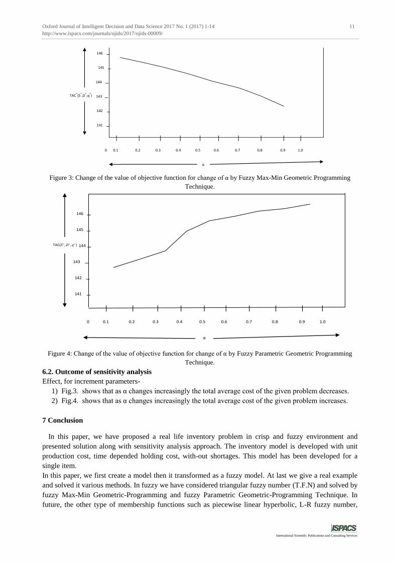
Figure 3: Change of the value of objective function for change of α by Fuzzy Max-Min Geometric Programming

Technique.

146 _

145 _

TAC(𝑆∗,𝐷∗, 𝑞∗) 144 _

143 _

142 _

141 _

| | | | | | | | | |

0 0.1 0.2 0.3 0.4 0.5 0.6 0.7 0.8 0.9 1.0

α

Figure 4: Change of the value of objective function for change of α by Fuzzy Parametric Geometric Programming

Technique.

6.2. Outcome of sensitivity analysis

Effect, for increment parameters-

1) Fig.3. shows that as α changes increasingly the total average cost of the given problem decreases.

2) Fig.4. shows that as α changes increasingly the total average cost of the given problem increases.

7 Conclusion

In this paper, we have proposed a real life inventory problem in crisp and fuzzy environment and

presented solution along with sensitivity analysis approach. The inventory model is developed with unit

production cost, time depended holding cost, with-out shortages. This model has been developed for a

single item.

In this paper, we first create a model then it transformed as a fuzzy model. At last we give a real example

and solved it various methods. In fuzzy we have considered triangular fuzzy number (T.F.N) and solved by

fuzzy Max-Min Geometric-Programming and fuzzy Parametric Geometric-Programming Technique. In

future, the other type of membership functions such as piecewise linear hyperbolic, L-R fuzzy number,




Trapezoidal Fuzzy Number (TrFN), Parabolic flat Fuzzy Number (PfFN), Parabolic Fuzzy Number (pFN),

pentagonal fuzzy number etc can be considered to construct the membership function and then model can

be easily solved.

Acknowledgements

The authors are thankful to University of Kalyani for providing financial assistance through DST-

PURSE Programme. The authors are grateful to the reviewers for their comments and suggestions

Reference

[1] R. E. Bellman, L. A. Zadeh, Decision making in a fuzzy environment, Management Science, 17 (1970)

B141-B164.

https://doi.org/10.1287/mnsc.17.4.B141

[2] B. Y. Cao, The further study of posynomial GP with Fuzzy co-e_cient, Mathematics Applicata, 5 (4)

(1992) 119-120.

[3] C. Carlsson, P. Korhonen, A parametric approach to fuzzy linear programming, Fuzzy sets and

systems, (1986) 17-30.

https://doi.org/10.1016/S0165-0114(86)80028-8

[4] A. J. Clark, An informal survey of multy-echelon inventory theory, naval research logistics Quarterly,

19 (2012) 621-650.

[5] D. Dutta, Pavan Kumar, Fuzzy inventory without shortages using trapezoidal fuzzy number with

sensitivity analysis, IOSR Journal of mathematics, 4 (3) (2012) 32-37.

https://doi.org/10.9790/5728-0433237

[6] D. Dutta, J. R. Rao, R. N. Tiwary, Effect of tolerance in fuzzy linear fractional Programming, Fuzzy

sets and systems, 55 (1993) 133-142.

https://doi.org/10.1016/0165-0114(93)90126-3

[7] R. J. Duffi, E. L. Peterson, C. M. Zener, Geometric programming- theory and applications, Wiley, New

York, (1967).

[8] Hamacher, H. Leberling, H. J. Zimmermann, Sensitivity Analysis in fuzzy linear Programming, Fuzzy

sets and systems, 1 (1978) 269-281.

https://doi.org/10.1016/0165-0114(78)90018-0

[9] G. Hadley, T. M. White, Analysis of inventory system, Prentice-Hall, Englewood Cliffs, Nj (1963).

[10] Kotb A.M Kotb, Hala A. Fergancy, Multi-item EOQ model with both demand-depended unit cost and

varying Leadtime via Geometric Programming, Applied mathematics, 2 (2011) 551-555.

https://doi.org/10.4236/am.2011.25072

[11] H.W Khun, A.W. Tucker, Non-linear programming, proceeding second Berkeley symposium

Mathematical Statistic and probability (ed) Nyman, J. University of California press, (1951) 481-492.

https://doi.org/10.1287/mnsc.17.4.B141

https://doi.org/10.1016/S0165-0114(86)80028-8

https://doi.org/10.9790/5728-0433237

http://dx.doi.org/10.1016/0165-0114(93)90126-3

https://doi.org/10.1016/0165-0114(78)90018-0

https://doi.org/10.4236/am.2011.25072




[12] H. X. Li, V. C. Yen, Fuzzy Sets and Fuzzy decision making, CRC press, London, (1995).

https://www.crcpress.com/Fuzzy-Sets-and-Fuzzy-Decision-Making/Li-Yen/p/book/9780849389313

[13] S. T. Liu, Posynomial geometric programming with interval exponents and Coefficients, European

Journal of Operational Research, 186 (1) (2008) 17-27.

https://doi.org/10.1016/j.ejor.2007.01.031

[14] M. K. Maity, Fuzzy inventory model with two ware house under possibility measure in fuzzy goal,

Euro. J. Oper. Res, 188 (1931) 746-774.


[15] F. E. Raymond, Quantity and Economic in manufacturing, McGraw-Hill, New York, (1931).

[16] S. Dey, T. K. Roy, Optimum shape design of structural model with imprecise coefficient by

parametric geometric programming, Decision Science Letters, 4 (2015) 407-418.

https://doi.org/10.5267/j.dsl.2015.3.002

[17] S. Islam, T. K. Roy, Modified Geometric programming problem and its applications, J. Appt. Math

and computing, 17 (1) (2005) 121-144.

https://doi.org/10.1007/BF02936045

[18] S. Islam, T. K. Roy, A fuzzy EPQ model with flexibility and reliability consideration and demand

depended unit Production cost under a space constraint: A fuzzy geometric programming approach,

Applied Mathematics and Computation, 176 (2) (2006) 531-544.

https://doi.org/10.1016/j.amc.2005.10.001

[19] S. Islam, T. K. Roy, Multi-Objective Geometric-Programming Problem and its Application, Yugoslav

Journal of Operations Research, 20 (2010) 213-227.

https://doi.org/10.2298/YJOR1002213I

[20] S. T. Liu, Posynomial Geometric-Programming with interval exponents and co-efficients, Europian

Journal of Operations Research, 168 (2) (2006) 345-353.


[21] T. K. Roy, M. Maity, A fuzzy inventory model with constraints, Opsearch, 32 (4) (1995) 287-298.

[22] W. A. Mandal, S. Islam, Fuzzy Inventory Model for Deteriorating Items, with Time Depended

Demand, Shortages, and Fully Backlogging, Pak.j.stat.oper.res, Vol. XII (1) (2016) 101-109.

http://dx.doi.org/10.18187/pjsor.v12i1.1153

[23] W. A.Mandal, S. Islam, Fuzzy Inventory Model for Power Demand Pattern with Shortages, Inflation

Under Permissible Delay in Payment, International Journal of Inventive Engineering and Sciences

(IJIES), 3 (8) (2015).

[24] W. A. Mandal, S. Islam, Fuzzy Inventory Model for Weibull Deteriorating Items, with Time

Depended Demand, Shortages, and Partially Backlogging, International Journal of Engineering and

Advanced Technology (IJEAT), 4 (5) (2015).

https://www.crcpress.com/Fuzzy-Sets-and-Fuzzy-Decision-Making/Li-Yen/p/book/9780849389313



https://doi.org/10.5267/j.dsl.2015.3.002

https://doi.org/10.1016/j.amc.2005.10.001

https://doi.org/10.2298/YJOR1002213I


http://dx.doi.org/10.18187/pjsor.v12i1.1153




[25] W. A.Mandal, S. Islam, Fuzzy unconstrained parametric geometric programming problem and

application, Journal of fuzzy set valued analysis, 2016 (2) (2016) 125-139.

https://doi.org/10.5899/2016/jfsva-00301

[26] W. A.Mandal, S. Islam, A Fuzzy Two-Warehouse Inventory Model for Weibull Deteriorating Items

with Constant Demand, Shortages and Fully Backlogging, International Journal of Science and

Research (IJSR), 4 (7) (2015).

[27] W. A.Mandal, S. Islam, Fuzzy E.O.Q model foe deteriorating items, with constant demand, shortages,

and fully Backlogging, Oxford Journal of Intelligent and Data Science, 2 (2016) 29-45.

https://doi.org/10.5899/2016/ojids-00006

[28] Y. Liang, F. Zhou, A two warehouse inventory model for deteriorating items under conditionally

permissible delay in Payment, Appl. Math. Model, 35 (2011) 2221-2231.

https://doi.org/10.1016/j.apm.2010.11.014

[29] L. A. Zadeh, Fuzzy sets, Information and Control, 8 (1965) 338-353.

https://doi.org/10.1016/S0019-9958(65)90241-X

[30] H. J. Zimmermann, Application of fuzzy set theory to mathematical programming, Information

Science, 36 (1985) 29-58.

https://doi.org/10.1016/0020-0255(85)90025-8

[31] H. J. Zimmermann, “Methods and applications of Fuzzy Mathematical programming”, in An

introduction to Fuzzy Logic Application in Intelligent Systems (R.R. Yager and L.A.Zadeh, eds),

(1992) 97- 120, Kluwer publishers, Boston.

https://doi.org/10.1007/978-1-4615-3640-6_5

https://doi.org/10.5899/2016/jfsva-00301

https://doi.org/10.5899/2016/ojids-00006

https://doi.org/10.1016/j.apm.2010.11.014

https://doi.org/10.1016/S0019-9958(65)90241-X

https://doi.org/10.1016/0020-0255(85)90025-8

https://doi.org/10.1007/978-1-4615-3640-6_5

A Fuzzy E.O.Q Model With Unit Production Cost, Time ... · YYYYYYYYYYYYYYYYY support Figure 2: Trapezoidal fuzzy number of 𝐴̃ with α-cuts. Aα is a non-empty bounded closed interval

Documents

A Fuzzy E.O.Q Model With Unit Production Cost, Time ... · YYYYYYYYYYYYYYYYY support Figure 2: Trapezoidal fuzzy number of 𝐴̃ with α-cuts. Aα is a non-empty bounded closed interval