A Constrained K-shortest Path Algorithm to Rank the Topologies of the Protein Secondary Structure Elements
Detected in CryoEM Volume Maps Kamal Al Nasr
Dept. of Computer Science Tennessee State University
3500 John A Merritt Blvd Nashville, TN 37209
Lin Chen, Desh Ranjan, M. Zubair, Dong Si, and Jing He
Dept. of Computer Science Old Dominion University
Norfolk, VA 23529
ABSTRACT
Although many electron density maps have been produced into
the medium resolutions, it is still challenging to derive the atomic
structure from such volumetric data. Current methods primarily
rely on the availability of an existing atomic structure for fitting or
a homologous template structure for modeling. In the process of
developing a template-free, de novo, method, the topology of the
secondary structure elements need to be resolved first. In this
paper, we extend our previous algorithm of finding the optimal
solution in the constraint graph problem. We illustrate an
approach to obtain the top-K topologies by combining a dynamic
programming algorithm with the K-shortest path algorithm. The
effectiveness of the algorithms is demonstrated from the test using
three datasets of different nature. The algorithm improves the
accuracy, space and time of an existing method.
Categories and Subject Descriptors
E.1 [Data Structures]: Arrays, Graphs and networks, Tables,
Trees. F.1.3 [Complexity Measures and Classes].
General Terms
Algorithms, protein, structure, 3-dimensional image.
Keywords
Electron cryomicroscopy, Graph, K-Shortest paths, Protein,
Topology, Algorithm.
1. INTRODUCTION Electron cryomicroscopy (CryoEM) is a biophysical technique
that has great potential in deriving the three-dimensional structure
of large protein complexes [3-6]. Various aspects in CryoEM have
been improved over the last ten years, and as a result, it is possible
to obtain the electron density maps of a protein in the high
resolution range, such as 3-5Å resolution [7-10]. At this
resolution, the connection between the secondary structures is
mostly distinguishable and the backbone of the structure can be
derived. The number of the atomic structures resolved from the
CryoEM density maps at the high resolution range steadily
increases in the last 3 years [11]. Some of these structures include
GroEL, virus and [5, 7, 8]. Although the structure determination
from high-resolution CryoEM maps is promising, a lot more
proteins are resolved at medium resolutions (5-10 Å resolutions)
than those at the high-resolution range. About 2/3 of the medium-
resolution maps have been resolved using fitting or template-
based homology modeling [12]. At this resolution range, the
location and the orientation of most secondary structures such as
helices and β-sheets are detectable using various computational
tools [2, 13-16]. A helix detected from the density map is
represented as a stick (red in Figure 1A) and a β-sheet appears as
a thin sheet (blue Figure 1A). Due to the medium resolution, the
strands of the β-sheet are often not distinguishable. The
connection between two SSEs is often ambiguous. The major
challenge to derive the protein structure from such CryoEM maps
is that it is not known which segment of the protein sequence
corresponds to which of the SSEs detected from the density map.
A topology of the SSEs refers to the order of the SSEs with
respect to the protein sequence and the direction of each SSE. For
example, the true topology of the protein in Figure 1 presents the
true order of the SSEs as
(Figure 1B). In
principle, each helix stick of the protein
corresponds to a sequence segment that forms a
helix in the structure. The four sequence segments and
correspond to a sheet that can be detected in the density map.
Note that there are two directions to correspond a sequence
segment to (arrows of Figure 1A and dot and cross in Figure
1B).
The medium-resolution density maps contain not only the
secondary structure location information but also the connecting
information among them. The skeleton (blue in Figure 2A) of a
density map represents the medial axis of the map. It can be
detected through a thinning and pruning process using Gorgon
[17]. When the detected secondary structure elements (red sticks
in Figure 2(a)) are overlaid with the skeleton (blue Figure 2a), the
connection relationship among them is reviewed. When the
resolution of the density map is at the medium resolution, the
skeleton can be misleading and incomplete, due to the
experimental factors. For example, the skeleton often contains
gaps (i.e. Figure 2(a)), and misleading points. Therefore, the
skeleton provides the connection information, but it is not
completely reliable.
The detected secondary structure elements (SSEs) provide
relative geometrical relationship among them. However, it is not
known which segment of the protein sequence corresponds to
which secondary structure element detected from the volumetric
density map. The topology of the SSEs refers to the order of the
Permission to make digital or hard copies of all or part of this work for
personal or classroom use is granted without fee provided that copies are not made or distributed for profit or commercial advantage and that
copies bear this notice and the full citation on the first page. To copy
otherwise, or republish, to post on servers or to redistribute to lists, requires prior specific permission and/or a fee.
Conference’10, Month 1–2, 2010, City, State, Country.
Copyright 2010 ACM 1-58113-000-0/00/0010 …$15.00.
ACM-BCB 2013 750
elements with respect to the protein sequence and the direction of
each element. To derive the backbone of the protein, the topology
of the secondary structures has to be determined first and then the
backbone of the protein can be built for further optimization [18-
20].
The topology determination problem combines two sources
of information. One source contains the detected secondary
structures, such as helix sticks (red Figure 1A), from the
volumetric map. The other source contains the predicted
secondary structures from the sequence (red, Figure 1C).
Many methods, such as PSIPRED [21], SSPRO [22] and
Porter [23], have been developed for the secondary structure
prediction from the amino acid sequence of a protein. In
general, the prediction accuracy of these methods is about 70-
80% [24]. Let be the helices of the amino acid
sequence in the protein. Due to the linear nature of the protein
sequence, the sequence segments have a fixed order
. Let { } be the set of sticks detected
from CryoEM volume map. In the context of this paper, we
assume , although vice versa is possible. The topology
determination problem can be described as problem of
matching to { }in an optimal way.
In the assignment, each is assigned to in one of the two
opposite directions. The total number of possible topologies is
( ) . For each sticks picked out of segments, there
are different orders and there are two directions to assign a
sequence fragment to each helix stick. When the assignment
involves -sheets, the total number of possible topologies
becomes (
) (
)
, in which and are the
number of sequence segments for helices and -strands
respectively, and similarly and are the number of the
detected helix and -stand sticks respectively.
Current approaches to find the best topology can be categorized
into three approaches. The direct approach enumerates all the
possible topologies of the SSEs and identifies the best by
comparing all of them [18, 25]. This approach has the limitation
of handling medium to large size proteins due to the huge solution
space. The largest number of secondary structures that can be
handled using a single desktop computer is about 9 helices [18].
Another approach uses Monte Carlo simulation to sample the
solution space [19]. Although this method can work with a large
solution space, the stochastic nature of the approach may miss the
native topology. The third, perhaps the most effective approach is
to translate the topology problem into a graph problem by
exploiting the constraints from a pair of sticks. Gorgon is such a
graph-matching method [26]. It produces two graphs, one
represents to the connectivity relationship of the sticks derived
from the volumetric map, and the other represents the linear
relationship of the segments on the proteins sequence. The
secondary structure assignment problem is then translated to an
inexact graph matching problem. Gorgon uses A* search in
matching the two graphs. The time complexity of A* depends on
the heuristics used. The worst case is the entire solutions space,
but often a significant portion of the entire space is explored.
We previously formulated the SSE topology problem into a
constraint graph problem and gave a dynamic programming
algorithm for the simplest situation in which [27]. More
importantly, our previous algorithm determines the optimal
solution that often fails when the optimal solution is not the true
topology due to the various errors in the data. We noticed that the
true topology is often near the top but not necessarily the top-1.
We illustrate an approach to find the top-K topologies using a
combination of a dynamic programming and the K-shortest paths
algorithms. In reality, determining the topology in a protein with
both α-helices and β-sheets is much harder, although the principle
is the same. The close positioning of the β-strands in a β-sheet
requires additional constraints from knowledge. On the other
hand, the quality of the skeleton plays an important role in the
quality of the results. In this paper, we will use a new tool to
extract the skeletons from CryoEM density maps (being
reviewed). The use of the new tool demonstrates that the quality
of the skeleton is one of the main factors to solve the problem of
the topology determination. Our fast algorithms make it possible
for a generic desktop computer to derive the true topologies
automatically for large proteins such as those containing 20-33
helices. This was not possible previously without user
intervention.
2. METHODS
2.1 Edge weight obtained from tracing the
skeleton
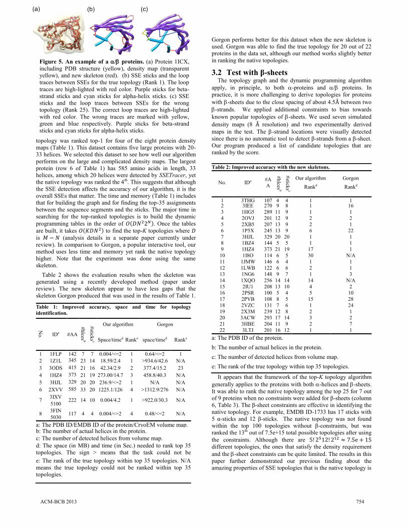
Figure 1. SSEs and the topology. (A) The density map (grey) was simulated to 10 Å resolution using protein 3PBA
from the Protein Data Bank (PDB) and EMAN software [1]. The SSEs (red: helix sticks, blue: sheet) were detected
using SSETracer, an extended version of Helix Tracer [2], and viewed by Chimera. For clear viewing, only SSEs at
the front of the structure are labeled. Arrows: the direction of the protein sequence; (B) The true topology of the sticks
(arrow, cross and dot for directions); (C) H1 to H10 : helix segments; E1 to E4: β-strands; ". . .": loops longer than 2
amino acids.
ACM-BCB 2013 751
We previously translated the SSE topology problem using a
weighted directed graph [27]. Briefly, there are
regular nodes in the graph, where is the number of SSE
segments on the protein sequence and is the number of SSE
sticks detected from the density map. Each node represents one
possible assignment between one SSE sequence segment and one
SSE stick in one of the two directions. Most of the edge weights
in the graph were assigned by tracing the skeleton. For any
possible edge, the weight of the edge is the absolute difference
between the virtual length of the loop (the number of Since the
skeleton contains the connection information between the SSEs,
the length from tracing the skeleton can be used as strong
constraints in matching the SSEs. However, the skeleton often
contains gaps and misleading points. In order to estimate the
length along the skeleton correctly, detailed analysis is needed.
The skeleton is represented as a set of voxel points. The main
idea of the tracing algorithm is to translate each voxel point at the
skeleton to a node in undirected graph. The voxel points (nodes)
represent the end of secondary structures are also marked. The
edges between any two nodes depend on the distance between the
two original voxel points. If the distance is less than 3.0 Å, the
two nodes are considered neighbors and an edge is created to
connect them. The weight of the edge equals to the distance
between the two corresponding voxel points. Bron-Kerbosch
algorithm [28] then applied to the graph to find the cliques of at
least size 3. The purpose of finding the cliques is to find the
crowded regions on the graph. The set of nodes involved in the
clique are replaced with one central node, the geometrical central
of all voxels of the clique. The depth first search (DFS) was used
to find the paths between a pair of ending points of two SSEs.
Some of the paths are complete paths. An incomplete path will be
found when a gap exists in the skeleton. For example, in Figure
2B, there are 3 complete paths from node P and one incomplete
path <P, R, S>. All paths found for each SSE end is saved in a
list 𝑒𝑛𝑑𝐿 𝑠𝑡 , where 𝑡 ∈ { }𝑎𝑛𝑑 ≤ ≤ . The variable 𝑡
represents which end on the stick the paths starts from. The length
of each path is simply the summation of weights of edges along
the path.
The process of edge update starts once all lists are built for all
SSE ends. For each edge 𝑒( 𝑡 𝑡 ) on the
graph, we find the complete path in 𝑒𝑛𝑑𝐿 𝑠𝑡 𝑡 or the two
incomplete paths in 𝑒𝑛𝑑𝐿 𝑠𝑡 𝑡 𝑎𝑛𝑑 𝑒𝑛𝑑𝐿 𝑠𝑡
𝑡 that best fit the
number of amino acids on the loop. 𝑡 is the complement
of 𝑡 denotes the other end of the stick . We simply search for a
complete or incomplete path with a length that best fit the
estimated length of the loop on the sequence. The estimated length
of the loop on the sequence is calculated by multiplying the
number of amino acids by 3.8. In both cases, complete or
incomplete, the length of the path should not exceed the estimated
length of the loop plus e=5 Å. Verifying complete paths against
loop is very simple. We trivially compare the two lengths. For
incomplete paths, we try all combination of incomplete paths
between the two lists that are at most 15Å apart. The length of the
new path produced from the two incomplete paths is the
summation of incomplete paths, one from each list, and the gap
between them. For example, in Figure 2B, the two incomplete
paths <P, R, S> and <T, Q> form one complete path <P, R, S, T,
Q>. The new weight of the edge is the absolute difference
between the length of the loop on the sequence and the best path
from the list. The weight of any edge does not have a proper path
(complete or incomplete) on the CryoEM volume map is changed
to ∞.
2.2 K-shortest paths satisfying the constraints The shortest valid path represents, in theory, the best match
between the SSEs on the protein sequence and those in the 3-
dimensional image. The K-shortest paths here refer to the K valid
paths, the score of which are in non-decreasing order. The main
constraint in the topology graph requires that a valid path cannot
visit the same row twice, neither can it visit the same column
twice. Due to the topology constraints, we cannot apply directly
the available K-shortest path algorithms. Instead, we combined the
concept of the “generalization of the Yen’s algorithm” of paper
[29] with our dynamic programming method to find the
constrained K-shortest paths.
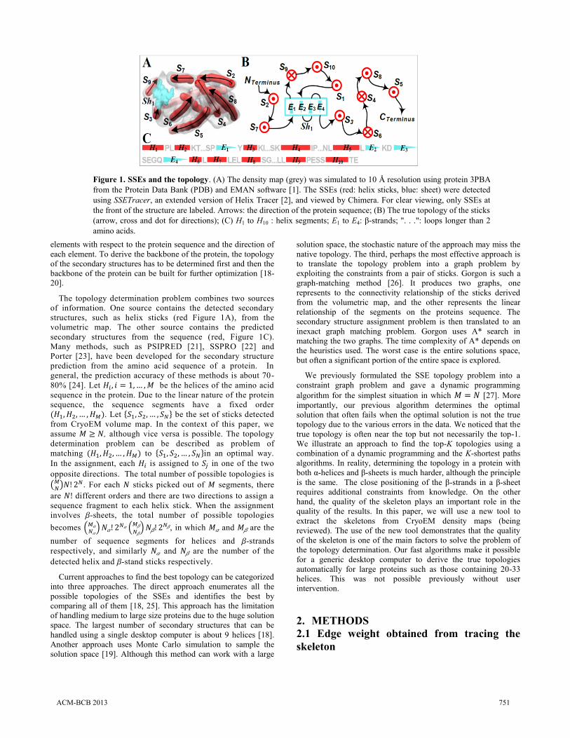
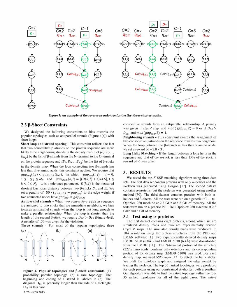
Let the th shortest valid path from <START> to <END> be
represented by
. Let
be the subpath of that includes the consecutive vertices of
between vertex and ≤ ≤ . In order to find
the -th shortest valid path, a “reverse pseudo tree” of the shortest valid paths, , is maintained. As mentioned in the
original K-shortest algorithm, is a pseudo tree because there
might be repeated nodes in the tree. We call it the reverse pseudo
tree since the root is in our case. The method to build
the pseudo tree was detailed in [29]. As an example (Figure 3), the
reverse pseudo tree maintains the “coninciding nodes” where
joins one of the paths and never deviates.
The idea of finding the next shortest path is that the th
shortest path is not too different from the previous shortest
paths. It is at least one edge different from each of the previous
shortest paths. At each cycle, new candidates for the th
shortest path are generated in an edge deletion process and are
deposited in , a set of the candidate paths. The th shortest
path is to be selected as the shortest path from X at iteration k+1.
Figure 2. The skeleton and tracing the skeleton to derive
the edge weight for the topology graph. A: The density map
(gray) of protein (PDB ID:3IXV_A) was extracted from the
entire density map (EMDB ID:5100) and is superimposed
with the skeleton (blue) and the true atomic structure (green
ribbon). The region of the skeleton containing gap is
highlighted with a box. B: Automatic tracing of skeleton to
overcome a gap between point S and point T.
A B
ACM-BCB 2013 752
2.3 β-Sheet Constraints
We designed the following constraints to bias towards the
popular topologies such as antiparallel strands (Figure 4(a)) with
short loops.
Short loop and strand spacing - This constraint reflects the fact
that two consecutive -strands on the protein sequence are more
likely to be neighboring strands in the density map. Let (E1, E2, ..,
) be the list of -strands from the N-terminal to the C-terminal
on the protein sequence and (B1, B2, .., ) be the list of -sticks
in the density map. When the loop connecting two β-strands has
less than five amino acids, this constraint applies. We require that
𝑎 𝑎 , in which 𝑎 ,
≤ ≤ ≤ and 𝑎 ⌊ ⌋ ≤
≤ . is a tolerance parameter. is the measured
shortest Euclidian distance between two -sticks Bk, and Bl. We
set a penalty of 𝑎 𝑎 to the edge weight if
two connected nodes have 𝑎 𝑎 .
Antiparallel strands - When two consecutive SSEs in sequence
are assigned to two sticks that are immediate neighbors, we bias
towards antiparallel strands when the loop is not long enough to
make a parallel relationship. When the loop is shorter than the
length of the second β-stick, we require (Figure 4(c)).
A penalty of 150 was given for the violation.
Three strands - For most of the popular topologies, three
consecutive strands form an antiparallel relationship. A penalty
was given if and 𝑑 or if
and 𝑑 𝑎 .
Neighboring strands - This constraint awards the assignment of
two consecutive β-strands on the sequence towards two neighbors.
When the loop between the β-strands is less than 5 amino acids,
we set a reward of .
Long Helix Matching - If the length between a long helix in the
sequence and that of the α-stick is less than 15% of the stick, a
reward of -5 was given.
3. RESULTS We tested the top-K SSE matching algorithm using three data
sets. The first data set contain proteins with only -helices and the
skeleton was generated using Gorgon [17]. The second dataset
contains -proteins, but the skeleton was generated using another
method [30]. The third dataset contains proteins with both -
helices and -sheets. All the tests were run on a generic PC – Dell
Optiplex 980 machine at 2.8 GHz and 8 GB of memory. All the
tests were run on a generic PC – Dell Optiplex 980 machine at 2.8
GHz and 8 GB of memory.
3.1 Test using α-proteins The first dataset contains eight proteins, among which six are
simulated density maps and two are experimentally derived
CryoEM maps. The simulated density maps were produced to
10Å resolution using the protein structures from the PDB and
EMAN software [1]. Two experimentally derived density maps
EMDB_5100 (6.8Å ) and EMDB_5030 (6.4Å) were downloaded
from the EMDB [11] . The N-terminal portion of the structure
(222 amino acids) contains only α-helices and its corresponding
portion of the density map (EMDB_5100) was used. For each
density map, we used SSETracer [13] to detect the helix sticks.
We built the topology graph and assigned the edge weight by
tracing the skeleton. The top 35 ranked topologies were produced
for each protein using our constrained K-shortest path algorithm.
Our algorithm was able to find the native topology within the top-
35 ranked topologies for all of the eight cases. The native
<START>
<END>
(1,1,1)
(2,2,1)
(5,3,0)
p1
<START>
<END>
(1,1,1)
(2,2,1)
(5,3,0)
p1q1p1 q2p1q3p1
Coin(q2p1)
C=6C=1 C=1
Coin(q3p1)
<START><START>
(4,2,1)
(2,1,0)(1,1,0)
C=2
Coin(q1p1)
<START>
(5,1,1)
(4,2,0)
(2,3,0)
C=2
<START>
<END>
(1,1,1)
(2,2,1)
(5,3,0)
p1q1p1 q2p1q3p1
Coin(q2p1)
C=6C=1
Coin(q3p1)
<START><START>
(4,2,1)
(2,1,0)(1,1,0)
C=2
Coin(q1p1)
<START>
(5,1,1)
(4,2,0)
(2,3,0)
C=2
p2
q2p2 q3p2
Coin(q2p2)
Coin(q3p2)
<START><START>
(3,3,1)
(1,2,1)
C=3
N/A
C=∞
(1,2,0)
<START>
Coin(q1p2)
(5,1,0)
(2,3,0)
q1p2C=2
p3p2
Figure 3: An example of the reverse pseudo tree for the first three shortest paths.
Figure 4. Popular topologies and -sheet constraints. (a)
probability popular topology; (b) a rare topology; The
beginning and ending of a strand is labeled in (c). The
diagonal DEE is generally longer than the side of a rectangle
DES in this case.
ACM-BCB 2013 753
topology was ranked top-1 for four of the eight protein density
maps (Table 1). This dataset contains five large proteins with 20-
33 helices. We selected this dataset to see how well our algorithm
performs on the large and complicated density maps. The largest
protein (row 6 of Table 1) has 585 amino acids in length, 33
helices, among which 20 helices were detected by SSETracer, yet
the native topology was ranked the 4th. This suggests that although
the SSE detection affects the accuracy of our algorithm, it is the
overall SSEs that matter. The time and memory (Table 1) includes
that for building the graph and for finding the top-35 assignments
between the sequence segments and the sticks. The major time in
searching for the top-ranked topologies is to build the dynamic
programming tables in the order of . Once the tables
are built, it takes to find the top-K topologies where
is (analysis details in a separate paper currently under
review). In comparison to Gorgon, a popular interactive tool, our
method uses less time and memory yet rank the native topology
higher. Note that the experiment was done using the same
skeleton.
Table 2 shows the evaluation results when the skeleton was
generated using a recently developed method (paper under
review). The new skeleton appear to have less gaps that the
skeleton Gorgon produced that was used in the results of Table 1.
Gorgon performs better for this dataset when the new skeleton is
used. Gorgon was able to find the true topology for 20 out of 22
proteins in the data set, although our method works slightly better
in ranking the native topologies.
3.2 Test with β-sheets The topology graph and the dynamic programming algorithm
apply, in principle, to both -proteins and / proteins. In
practice, it is more challenging to derive topologies for proteins
with -sheets due to the close spacing of about 4.5 between two
-strands. We applied additional constraints to bias towards
known popular topologies of -sheets. We used seven simulated
density maps (8 resolution) and two experimentally derived
maps in the test. The -strand locations were visually detected
since there is no automatic tool to detect β-strands from a β-sheet.
Our program produced a list of candidate topologies that are
ranked by the score.
It appears that the framework of the top-K topology algorithm
generally applies to the proteins with both -helices and -sheets.
It was able to rank the native topology among the top 25 for 7 out
of 9 proteins when no constraints were added for β-sheets (column
6, Table 3). The β-sheet constraints are effective in identifying the
native topology. For example, EMDB ID-1733 has 17 sticks with
5 α-sticks and 12 β-sticks. The native topology was not found
within the top 100 topologies without β-constraints, but was
ranked the 13th out of 7.5e+15 total possible topologies after using
the constraints. Although there are
different topologies, the ones that satisfy the density requirement
and the -sheet constraints can be quite limited. The results in this
paper further demonstrated our previous finding about the
amazing properties of SSE topologies that is the native topology is
Table 1: Improved accuracy, space and time for topology
identification.
No
. IDa #AA
#hlces
b
#stick
sc
Our algorithm Gorgon
Space/timed Ranke space/timed Ranke
1 1FLP 142 7 7 0.004/<=2 1 0.64/<=2 1
2 1Z1L 345 23 14 18.59/2.4 1 >934.6/42.6 N/A
3 3ODS 415 21 16 42.34/2.9 2 377.4/15.2 23
4 1HZ4 373 21 19 273.00/14.7 3 458.8/40.3 N/A
5 3HJL 329 20 20 236.9/<=2 1 N/A N/A
6 2XVV 585 33 20 1225.1/126 4 >1312.9/276 N/A
7 3IXV
222 14 10 0.004/4.2 1 >922.0/30.3 N/A 5100
8 3FIN
117 4 4 0.004/<=2 4 0.48/<=2 N/A 5030
a: The PDB ID/EMDB ID of the protein/CryoEM volume map. b: The number of actual helices in the protein.
c: The number of detected helices from volume map.
d: The space (in MB) and time (in Sec.) needed to rank top 35
topologies. The sign > means that the task could not be
completed. e: The rank of the true topology within top 35 topologies. N/A
means the true topology could not be ranked within top 35
topologies.
Table 2: Improved accuracy with the new skeletons.
No. IDa #A
A
#hlces
b
#stick
sc
Our algorithm
Rankd
Gorgon
Rankd
1 3THG 107 4 4 1 1 2 3IEE 270 9 8 1 16
3 1HG5 289 11 9 1 1
4 2OVJ 201 12 9 2 2
5 2XB5 207 13 9 2 1
6 1P5X 245 13 9 6 22
7 3HJL 329 20 20 1 1
8 1BZ4 144 5 5 1 1
9 1HZ4 373 21 19 17 1
10 1I8O 114 6 5 30 N/A
11 1JMW 146 6 4 1 1
12 1LWB 122 6 6 2 1
13 1NG6 148 9 7 1 3
14 1XQO 256 14 14 14 N/A
15 2IU1 208 13 10 4 2
16 2PSR 100 5 4 5 10
17 2PVB 108 8 5 15 28
18 2VZC 131 7 6 1 24
19 2X3M 239 12 8 2 1
20 3ACW 293 17 14 3 2
21 3HBE 204 11 9 2 7
22 3LTJ 201 16 12 1 1
a: The PDB ID of the protein.
b: The number of actual helices in the protein.
c: The number of detected helices from volume map.
e: The rank of the true topology within top 35 topologies.
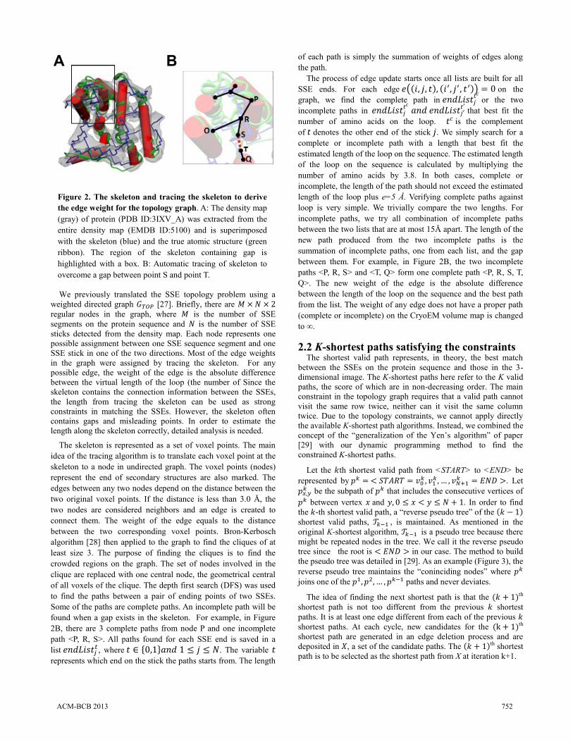
Figure 5. An example of a / proteins. (a) Protein 1ICX,
including PDB structure (yellow), density map (transparent
yellow), and new skeleton (red). (b) SSE sticks and the loop
traces between SSEs for the true topology (Rank 1). The loop
traces are high-lighted with red color. Purple sticks for beta-
strand sticks and cyan sticks for alpha-helix sticks. (c) SSE
sticks and the loop traces between SSEs for the wrong
topology (Rank 25). The correct loop traces are high-lighted
with red color. The wrong traces are marked with yellow,
green and blue respectively. Purple sticks for beta-strand
sticks and cyan sticks for alpha-helix sticks.
ACM-BCB 2013 754
near the top of the entire topological space [31]. Figure 5 shows
an example of the correct and incorrect topology.
4. CONCLUSION The topology of the secondary structure elements detected from
the density map is a critical piece of information for deriving the
atomic structures from such density maps. This paper illustrated
the K-shortest paths approach to the SSE topology problem. The
algorithms were tested using data sets involving proteins with
large number of SSEs in both α-proteins and α/β proteins. The
effectiveness of the algorithms was demonstrated in the ability of
ranking the native topologies to the near top for α-proteins up to
33 helices in which 20 of them were detected in the density map
and α/β-proteins up to 12 β-strands and 5 α-helices. The results
represent a major improvement in the ability to derive the
secondary structure topology automatically for large and
complicated density maps.
5. ACKNOWLEDGMENT Correspondence to: Jing He, [email protected].
The funding of this work is in part by NSF-CREST HRD-
0420407, the start-up fund and MSF fund of Old Dominion
University.
6. REFERENCES [1] Ludtke, S. J., Baldwin, P. R. and Chiu, W. EMAN: Semi-
automated software for high resolution single particle
reconstructions. Journal of Structural Biology, 128, 1 1999), 82-
97.
[2] Del Palu, A., He, J., Pontelli, E. and Lu, Y. Identification of
Alpha-Helices from Low Resolution Protein Density Maps.
Proceeding of Computational Systems Bioinformatics
Conference(CSB)2006), 89-98.
[3] Chiu, W. and Schmid, M. F. Pushing back the limits of
electron cryomicroscopy. Nature Struct. Biol., 41997), 331-333.
[4] Zhou, Z. H., Dougherty, M., Jakana, J., He, J., Rixon, F. J. and
Chiu, W. Seeing the herpesvirus capsid at 8.5 A. Science, 288,
5467 (May 5 2000), 877-880.
[5] Ludtke SJ, C. D., Song JL, Chuang DT, Chiu W. Seeing
GroEL at 6 A resolution by single particle electron
cryomicroscopy. Structure, 12, 7 (Jul 2004), 1129-1136.
[6] Chiu, W., Baker, M. L., Jiang, W. and Zhou, Z. H. Deriving
folds of macromolecular complexes through electron
cryomicroscopy and bioinformatics approaches. Curr Opin Struct
Biol, 12, 2 (Apr 2002), 263-269.
[7] Yu, X., Jin, L. and Zhou, Z. H. 3.88A structure of cytoplasmic
polyhedrosis virus by cryo-electron microscopy. Nature, 453,
7193 (05/15/print 2008), 415-419.
[8] Cong, Y., Baker, M. L., Jakana, J., Woolford, D., Miller, E. J.,
Reissmann, S., Kumar, R. N., Redding-Johanson, A. M., Batth, T.
S., Mukhopadhyay, A., Ludtke, S. J., Frydman, J. and Chiu, W.
4.0-Å resolution cryo-EM structure of the mammalian chaperonin
TRiC/CCT reveals its unique subunit arrangement. Proceedings of
the National Academy of Sciences, 107, 11 (March 16, 2010
2010), 4967-4972.
[9] Zhang, X., Jin, L., Fang, Q., Hui, W. H. and Zhou, Z. H. 3.3 Å
Cryo-EM Structure of a Nonenveloped Virus Reveals a Priming
Mechanism for Cell Entry. Cell, 141, 3 (April 2010 2010), 472-
482.
[10] Baker, M. L., Zhang, J., Ludtke, S. J. and Chiu, W. Cryo-EM
of macromolecular assemblies at near-atomic resolution. Nat.
Protocols, 5, 10 (09//print 2010), 1697-1708.
[11] Lawson, C. L., Baker, M. L., Best, C., Bi, C., Dougherty, M.,
Feng, P., van Ginkel, G., Devkota, B., Lagerstedt, I., Ludtke, S. J.,
Newman, R. H., Oldfield, T. J., Rees, I., Sahni, G., Sala, R.,
Velankar, S., Warren, J., Westbrook, J. D., Henrick, K.,
Kleywegt, G. J., Berman, H. M. and Chiu, W. EMDataBank.org:
unified data resource for CryoEM. Nucleic Acids Research, 39,
suppl 1 (January 1, 2011 2011), D456-D464.
[12] Henderson, R., Sali, A., Baker, Matthew L., Carragher, B.,
Devkota, B., Downing, Kenneth H., Egelman, Edward H., Feng,
Z., Frank, J., Grigorieff, N., Jiang, W., Ludtke, Steven J., Medalia,
O., Penczek, Pawel A., Rosenthal, Peter B., Rossmann,
Michael G., Schmid, Michael F., Schröder, Gunnar F., Steven,
Alasdair C., Stokes, David L., Westbrook, John D., Wriggers, W.,
Yang, H., Young, J., Berman, Helen M., Chiu, W., Kleywegt,
Gerard J. and Lawson, Catherine L. Outcome of the First Electron
Microscopy Validation Task Force Meeting. Structure, 20, 2
2012), 205-214.
[13] Si, D., Ji, S., Al Nasr, K. and He, J. A machine learning
approach for the identification of protein secondary structure
elements from CryoEM density maps. Biopolymers, 972012),
698-708.
[14] Baker, M. L., Ju, T. and Chiu, W. Identification of secondary
structure elements in intermediate-resolution density maps.
Structure, 15, 1 (Jan 2007), 7-19.
[15] Jiang, W., Baker, M. L., Ludtke, S. J. and Chiu, W. Bridging
the information gap: computational tools for intermediate
resolution structure interpretation. J Mol Biol, 308, 5 (May 2001),
1033-1044.
[16] Kong, Y., Zhang, X., Baker, T. S. and Ma, J. A Structural-
informatics approach for tracing beta-sheets: building pseudo-
C(alpha) traces for beta-strands in intermediate-resolution density
maps. J Mol Biol, 339, 1 (May 21 2004), 117-130.
[17] Baker, M. L., Abeysinghe, S. S., Schuh, S., Coleman, R. A.,
Abrams, A., Marsh, M. P., Hryc, C. F., Ruths, T., Chiu, W. and
Ju, T. Modeling protein structure at near atomic resolutions with
Gorgon. Journal of Structural Biology, 174, 2 2011), 360-373.
Table 3. The evaluation of / proteins.
ID/EMDB
#H
elicesa
#S
trand
b
Sh
eet_ID
c
#T
otal
d
NO
PT
e
Ran
kf
5030 4/3 4/3 A 3.7e+04 1 1
1733 5/5 12/12 O,P,Q 7.5e+15 -/100 13
1OZ9 5/5 5/4 A 7.7e+05 25 7
2KUM 2/2 3/3 A 3.8e+02 5 1
2KZX 3/3 3/3 A 2.3e+03 10 10
2L6M 2/2 3/3 A 3.8e+02 6 6
1BJ7 5/1 9/9 A 1.9e+09 -/100 4
1ICX 6/3 7/7 A 6.2e+08 2 1
1JL1 4/4 5/5 A 1.5e+06 22 16
a: The number of -helices in the protein sequence and the
number of -sticks detected from the density map;
b: The number of -strands in the protein sequence and the
number of -strands visually detected;
c: -Sheet ID;
d: The number of total possible topologies;
e: The rank of the native topology without β-constraints; -
/100: the native topology not found in top 100 topologies
f: The rank of the native topology with β-constraints
ACM-BCB 2013 755
[18] Al Nasr, K., Sun, W. and He, J. Structure prediction for the
helical skeletons detected from the low resolution protein density
map. BMC Bioinformatics, 11, Suppl 1 (January 2010 2010), S44.
[19] Lindert, S., Staritzbichler, R., Wötzel, N., Karakaş, M.,
Stewart, P. L. and Meiler, J. EM-Fold: De Novo Folding of α-
Helical Proteins Guided by Intermediate-Resolution Electron
Microscopy Density Maps. Structure, 17, 7 (July 2009 2009),
990-1003.
[20] Lindert, S., Alexander, N., Wötzel, N., Karaka, M., Stewart,
Phoebe L. and Meiler, J. EM-Fold: De Novo Atomic-Detail
Protein Structure Determination from Medium-Resolution
Density Maps. Structure, 20, 3 2012), 464-478.
[21] Jones, D. T. Protein secondary structure prediction based on
position-specific scoring matrices. J Mol Biol, 292, 2 (Sep 1999),
195-202.
[22] Cheng, J., Randall, A. Z., Sweredoski, M. J. and Baldi, P.
SCRATCH: a protein structure and structural feature prediction
server. Nucleic Acids Research, 33, suppl 2 (July 1, 2005 2005),
W72-W76.
[23] Pollastri, G. and McLysaght, A. Porter: a new, accurate
server for protein secondary structure prediction. Bioinformatics,
21, 8 (Apr 15 2005), 1719-1720.
[24] Ward, J. J., McGuffin, L. J., Buxton, B. F. and Jones, D. T.
Secondary structure prediction with support vector machines.
Bioinformatics, 19, 13 (Sep 1 2003), 1650-1655.
[25] Wu, Y., Chen, M., Lu, M., Wang, Q. and Ma, J. Determining
protein topology from skeletons of secondary structures. J Mol
Biol, 350, 3 (Jul 15 2005), 571-586.
[26] Abeysinghe, S., Ju, T., Baker, M. L. and Chiu, W. Shape
modeling and matching in identifying 3D protein structures.
Computer-Aided Design, 40, 6 2008), 708-720.
[27] Al Nasr, K., Ranjan, D., Zubair, M. and He, J. Ranking Valid
Topologies of the Secondary Structure elements Using a
constraint Graph. Journal of Bioinformatics and Computational
Biology, 9, 3 2011), 415-430.
[28] Bron, C. and Kerbosch, J. Algorithm 457: finding all cliques
of an undirected graph. Communications of the ACM, 16, 9 1973),
575-577.
[29] Martins, E. d. Q. V., Pascoal, M. M. B. and Santos, J. L. E. d.
Deviation Algorithms for Ranking Shortest Paths. International
Journal of Foundation of Computer Science, 10, 3 1999), 247-
263.
[30] Al Nasr, K., Liu, C., Rwebangira, M., Burge, L. and He, J.
Intensity-based skeletonization of CryoEM grayscale images
using a true segmentation-free algorithm. IEEE Transactions on
Computational Biology and Bioinformatics2013 (Under Review).
[31] Sun, W. and He, J. Native secondary structure topology has
near minimum contact energy among all possible geometrically
constrained topologies. Proteins: Structure, Function, and
Bioinformatics, 77, 1 (October 2009 2009), 159-173.
ACM-BCB 2013 756