A comparison of clustering heuristics for scheduling dags on multiprocessors

JOURNAL OF PARALLEL AND DISTRIBUTED COMPUTING 16, 276-291 (1992)

A Comparison of Clustering Heuristics for Scheduling Directed Acyclic Graphs on Multiprocessors

APOSTOLOS GERASOULIS AND TAO YANG

Clustering of task graphs has been used as an intermediate step toward scheduling parallel architectures. In this paper, we identify important characteristics of clustering algorithms and propose a general framework for analyzing and evaluating such algorithms. Using this framework, we present an analytic performance comparison of four algorithms: Dominant Sequence Clus- tering (DSC) (Yang and Gerasoulis, Proc. Super-computing ‘91, 1991, pp. 633-642) and the algorithms of Kim and Browne (Znt. Conf. on Parallel Processing, 1988, Vol. 3, pp. l-8), Sarkar (Par- titioning and Scheduling Parallel Programs for Execution on Multiprocessors, MIT Press, 1989), and Wu and Gajski (J. Super- comput. 2 (1988), 349-372). We identify the common features and differences of these algorithms and explain why DSC is superior to other algorithms. Finally, we present some experiments to verify our analysis. 8 WE Academic Press, Inc.

1. INTRODUCTION

In this paper, we consider the clustering problem for directed acyclic graphs (DAGs). Clustering is a mapping of the nodes of a DAG onto labeled clusters. A cluster consists of a set of tasks; a task is an indivisible unit of computation. All tasks in a cluster must execute in the same processor. The clustering problem has been shown to be NP-complete for a general task graph and for several cost functions. For example, if the cost function is the minimization of parallel time on a completely connected virtual architecture with an unbounded number of processors, then clustering is NP-hard in the strong sense (Sarkar [ 141, Chretienne [ 11, Papadimitriou and Yannaka- kis [13]).

Several heuristic algorithms have been proposed in the literature for the general clustering problem. Kim and Browne [lo] considered linear clustering, which is an important special case of clustering. Sarkar [ 141 presented a clustering algorithm based on a scheduling algorithm on unbounded number of processors. Wu and Gajski [I71 developed a programming aid for hypercube architectures using scheduling techniques. Yang and Gerasoulis [15, 161 proposed a fast and accurate heuristic algorithm, the Dominant Sequence Clustering (DSC). However, there has been little experimental and theoretical comparisons of clustering algorithms. One exception is the

recent paper by El-Rewini and Lewis [3], where experiments with some scheduling algorithms are presented. Here, we introduce a general analytic framework and use it to express clustering heuristics so that comparisons can be made in a systematic fashion. The paper is organized as follows:

In Section 2, we describe the basic terminology and assumptions used in clustering and scheduling algorithms. In Section 3, we introduce a generic framework that visualizes a clustering algorithm as performing a sequence of clustering refinements so that a clustering algorithm can be presented in a systematic manner. In Sec- tion 4, we describe the important characteristics and performance features of clustering algorithms so that we can clarify the differences and similarities and evaluate their performance through this framework. In Section 5, we present four algorithms using our framework, and use an example to demonstrate their clustering steps. In Sec- tion 6, we study their performance for special important primitive classes of DAGs such as fork, join, and coarse grain trees. These are DAGs whose optimal solutions can be computed in polynomial time. In Section 7, we present experimental results that verify our analytic results. Sec- tion 8 is the conclusion.

2. PROBLEM DEFINITION AND ASSUMPTIONS

We start with definitions of the task computation model and architecture:

A directed acyclic weighted task graph (DAG) is de- finedbyatupleG=(V,E,%,~)whereV={n;,j= 1: u} is the set of task nodes and u = /VI is the number of nodes, E is the set of communication edges and e = IEl is the number of edges, % is the set of edge communication costs, and 5 is the set of node computation costs. The value c;,j E % is the communication cost incurred along the edge ei,.i = (n;, prj) E E, which is zero if both nodes are mapped in the same processor. The value 7; E 9 is the execution time of node n; E V.

A task is an indivisible unit of computation which may be an assignment statement, a subroutine or even an en- tire program. The tasks are convex, which means that once a task starts its execution it can run to completion without interruption (Sarkar [ 141).

276

0743.73 IS/92 $5.00 Copyright 0 1992 by Academic Press. Inc. All rights of reproduction in any form reserved.

CLUSTER HEURISTICS FOR SCHEDULING DAGS 277

The task execution model is the static macro-dataflow model (Sarkar [14], Wu and Gajski [17], El-Rewini and Lewis [3]). The task execution is triggered by the arrival of all data from its predecessors. Immediately after completion of task execution, the data are sent to the successor tasks. Data communication is done in parallel.

The architecture is a completely connected graph, with an unbounded number of homogeneous processors, i.e., a clique virtual architecture.

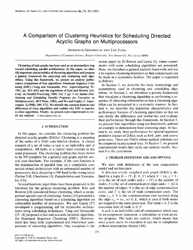
Clustering is a mapping of the tasks of a DAG onto clusters. A cluster is a set of tasks which will execute on the same processor. Clustering is also known as processor assignment in the case of an unbounded number of processors on a clique architecture (Sarkar [ 141). Cluster- ing has been shown to be NP-complete for the minimization of the parallel time cost function (Chretienne [I], Papadimitriou and Yannakakis [ 131, Sarkar [ 141). As a result many heuristic algorithms have been proposed and analyzed in the literature. A clustering is called nonlinear if two independent tasks are mapped in the same cluster; otherwise it is called linear. In Fig. la we give a weighted DAG, in lb a linear clustering with three clusters {n, , nz, ~7). {n3, n4, n6}, {no}, and in lc a nonlinear clustering with clusters {ni , n:}, {n?, n4, n5, n6}, and {n,}. Note that for the nonlinear cluster the independent tasks n4 and tz5 are mapped into the same cluster.

Scheduling is a task to processor assignment and a tusk to starting time mapping. In general, the problem of finding the optimum scheduling that minimizes the parallel time has been shown to be NP-complete (Sarkar [ 141). In Fig. 2b we present the Gantt chart of a schedule for the nonlinear clustering of Fig. lc. Processor PO has tasks nl and n2 with starting times ST(n,) = 0 and ST(+) = 1. If we modify the clustered DAG as in [14] by adding zero- weighted edges between any pair of two nodes II, and II, of a cluster, if n, is executed immediately after n,, and if there is no data dependence edge between n, and n!, then we obtain what we call a scheduled DAG; see 2c. We call the longest path of the scheduled DAG the dominant sequence (DS 1 of the clustered DAG, to distinguish it from

FIG. 1. (a) A weighted DAG: (b) a linear clustering; (c) a nonlinear clustering.

PO PI p2

Time

FIG. 2. (a) The clustered DAG and its CP shown in thick arrows; (b) the Gantt chart of a schedule: (c) the scheduled DAG and the DS shown in thick arrows.

the critical path (CP) of a clustered but not scheduled DAG. For example, the clustered DAG of Fig. la also shown in Fig. 2a has CP = (n, , n2, n7) with length 9, while a DS of a schedule given in Fig. 2c is DS = (n, , n3, n4, n5, nh, n,> and has length 10. In the case of linear clustering, the DS and CP of the clustered DAG are iden- tical; see Fig. lb.

Clustering has been used as a first step to scheduling parallel architectures. More specifically, Sarkar [14], who calls clustering “internalization prepass,” proposes a two step method for scheduling: (1) Perform clustering by scheduling on an unbounded number of processors of a clique. (2) Merge and schedule the clusters when the number of processors is smaller than the number of clusters. Sarkar gives the following justification for clustering: “If tasks are scheduled in the same processor on the best possible architecture with an unbounded number of processors, then they should be scheduled in the same processor in any other architecture.” Other areas in the literature where clustering has been used are the VLSI systolic schedules (Kung [I l]), where the clustering step is known as the processor projection step, and numerical computing for message passing architectures (Ortega [la).

3. A GENERIC DESCRIPTION OF CLUSTERING

ALGORITHMS

Clustering heuristics have certain goals and try to achieve them via a sequence of steps. Clustering algorithms perform a sequence of refinement steps opi, i = 0 : k. An initial clustering is given in opo. Here we us- sume that initially each task is a cluster. Each op; performs a refinement of the previous clustering by merging some clusters and at the last step opk, a final clustering is derived. At each step a good refinement must be performed so that the final clustering satisfies or is

278 GERASOULISANDYANG

“close” to satisfying the original goals. We only consider nonbacktracking heuristic algorithms to avoid high complexity; i.e., once the clusters have been merged in (Ipi they cannot be unmerged afterwards. Then the number of clustering steps remains polynomially bounded with re- spect to the size of the DAG.

Let us demonstrate how the nonlinear clustering in Fig. lc could be derived as a sequence of merging operations op,. We use the criterion that “two clusters are merged if the parallel time does not increase.” Initially each task is mapped to a separate cluster shown in Fig. 1 a and the parallel time is equal to 14, which is the length of ml = (n, , e, n7). The first step merges nl and n2 and renames the resulting cluster as 1. Then DS, = (n, , n3, n4 3 & 3 n,) and the parallel time reduces to 13.5. In the next step clusters n3 and n4 are merged and renamed cluster 2. Then DSz = (n, , n3, n5, n6, n7) and the parallel time reduces to 12.5. In the third step clusters ns and n6 are merged to become cluster 3. Then DS3 = (n, , n3, n5, nb, 1~) and the parallel time reduces to 10. In the final step clusters 2 and 3 are merged. Since n4 and n5 are two independent tasks assigned in the same processor an ordering must be used to determine the parallel time. In this case the parallel time remains equal to 10 if n4 is executed before n3 or vice versa.

Several interesting observations can be made: (I) When two clusters are merged, a scheduling heuristic might be needed to determine the new parallel time and measure the performance. (2) If there exists a nonzero edge connecting two clusters, then merging the two clusters will zero the edge cost. Equivalently, zeroing an edge cost will merge two clusters. (3) If there is no edge connecting two clusters then the parallel time cannot be reduced by merging these clusters, but it might be in- creased by such a merging because of sequentialization of independent tasks. (4) If zeroing the edges connecting two linear clusters results in a linear cluster, then such a merging will not increase the parallel time. If such a zeroing results in a nonlinear cluster, then the reduction or not of the parallel time will depend on the granularity of the DAG [6].

3.1. Clustering Algorithms Based on Edge-Zeroing

The edge-zeroing based merging algorithms constitute an important subclass of clustering algorithms which we will study in detail. Such algorithms only operate on the connected component of the DAG and never merge tasks that are not connected. Edge-zeroing clustering will produce a sequence of graph transformations Gi = ( V, E, %;, %), i = 0 : k of the initial DAG. The operation op, only modifies the set ‘%-I to %; by edge zeroing while the sets V, E, and 9 remain unchanged. For edge-zeroing clustering algorithms, we define:

T “2 “k “m “I “2 “k “k+l “m

a Fork DAG b Clustered DAG

FIG. 3. Clustering a fork DAG

l CLU-HEU: The CLUstering HEUristic which se- lects the edges to be zeroed.

l SCH-ALG: The SCHeduling ALGorithm. l domain(opi): The set of edges in E to be examined by

OPi.

l focus(op;): The set of edges that are candidates for zeroing at opi.

l zevo(op;): The set of edges that will be zeroed at the completion of 0~;.

l SG;: The scheduled DAG according to SCH-ALG. Initially, SGo = Go.

l DS;: The Dominant Sequence at the completion of opi, which is the critical path of SGi.

l CP;: The set of all nodes in the Critical Path of Gj = (V, E, %i, 3). i = 0 : k.

l top-leuel(n.,., i), hot-leuel(n,, i): The length of the longest path between node IZ., and the top (bottom) node in SG;, including all the communication and computation costs in that path, but excluding 7, from top-leuel(n., , i).

l PTi: The Parallel Time at the completing of op;.

PTi = 2 Tj + 2 Cj, , , , = top-/eve/( n,x, i) ll,ED.S, “I,. !I,,,EDJ,

+ hot-leuehn,, i), n, E DSi.

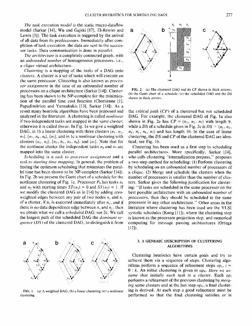
Let us now consider a fork DAG F., with communication Costs c.,,,, = fij, j = I : m shown in Fig. 3a to demonstrate an edge-zeroing clustering sequence. We present an optimum clustering algorithm for a fork DAG in Fig. 4. For simplicity we assume that the nodes and edges have been sorted such that Tj + fij 2 ~i+l + pi-1 , j = I : m - I.

i = 1.

PT; = m+Cj=* Tjj,C+l t &+I) t Tz ENDWHILE k=i-1:

FIG. 4. An optimum clustering algorithm for a fork DAG.


CLUUEU : Minimize the parallel time.

SCHALG: Any ordering of ~lr nz,. , R; results in an optimal schedule.

focus(op;) = {< n,, 7% >}.

constraint: PT, 5 PTi-1.

tero(op;) = focus(op;) if constsaint is true otherwise 0.

Termination criterion: When constraint is not true.

FIG. 5. Edge zeroing operations in the fork clustering algorithm.

Initially each task is mapped onto a separate processor of the clique. At each step i of the algorithm, corresponding to opi, the focus is on the edge (n, , n;) and if the parallel time reduces by zeroing that edge then this edge is zeroed, see Fig. 3b. Therefore, the task rzj,j = 1 : i will be mapped in the same cluster if PT, 5 PT;-, . A summary of the algorithm is given in Fig. 5. The proof of optimality is given in [1.5], Theorem 4.2.

4. A CHARACTERIZATION OF CLUSTERING ALGORITHMS

Clustering Goals and Cost Functions. Clustering heuristics must have certain goals and must choose the corresponding cost functions for achieving those goals. We distinguish between two types of goals, the perfou- ITZUIZC~ type and the nonperformance type. Performance goals could be the following: (Gl) Minimization of the parallel time cost function on an unbounded number of processors. (G2) Maximization of the efficiency cost function. (G3) Minimization of the communication volume, CV = C r,,,eEC’i,jr cost function. Nonperformance goals, on the other hand, impose constraints on the structure and shape of the clustering rather than its performance. Examples are: (G4) Clustering is linear. (G5) Clusters have no cycles; i.e., they are convex (Sarkar [14]). (G6) Clustering satisfies the locality of data assumption [4].

One can use a combination of goals as long as they do not conflict with each other. Whenever conflicts occur, then a goal priority must be imposed. For example, G41 GI implies that G4 will be used first when there is a conflict and the result will be an optimum linear clustering. On the other hand, if we use GIIG4, the primary goal Gl could lead to nonlinear clusters if the corresponding parallel time is shorter. G2 and G3 alone are not reasotl- ah/e goals, unless combined with another goal or constraint, since maximization of the efficiency and minimization of communication volume can both be achieved by mapping all nodes to a single cluster.

Goal Transform&ion. Because of the NP-complete- ness of the problems that have some of the above goals, these problems cannot be solved in polynomial time. Therefore, the goals must be transformed so that their cost functions are directly computable in polynomial time. For example, the goal for our optimum fork clustering algorithm in the last section is Gl. Because of the special structure of the graph, the goal is equivalent to solving

Thus the new transformed goal becomes the minimization of the last function, which can be achieved by zeroing pi+, whenever T;+, + pi+, is the maximum above. Re- peating such zeroing yields an optimal zeroing sequence which satisfies PTO 2 PTI Z- ... z PTA and PTk < PTk+, . It just happened for this example that the achievement of the transformed goal also implies the achievement of the original goal. This is not true in general.

Another example of goal transformation is Sarkar’s algorithm [14] which has as a primary goal Gl. His transformed goal is “the minimization of communication volume G3 without increasing the parallel time.”

Performance Features. What are the special features that warrant good performance of clustering algorithms? Because the clustering problem is NP-complete for the performance goals Gl /G2, it is extremely difficult to find the features that will warrant optimum clusterings. There are certain features, however, which we believe are necessary to ensure good performance of clustering algorithms:

Monotonic decrease of parallel time. Let us consider the nonbacktracking clustering algorithms. To ensure that such algorithms produce a clustering whose parallel time is not worse than the initial parallel time, a safeguard must be imposed. One such safeguard is the nonincrease of the parallel time at each step of the algorithm:

(Tl) PT; % PT;-, .

This condition ensures that at least a local minimum of the parallel time of a clustering sequence will be derived. As a matter of fact if the task graph is coarse-grained any local minimum of a clustering algorithm that satisfies Tl will be within a factor of two of the optimum clustering. This is because for coarse-grained graphs every linear clustering is within a factor of two of the optimum: see [5, 61. Since the initial clustering is linear, Tl ensures that the parallel time does not increase. Thus, Tl is a reason- able constraint at least for coarse-grained DAGs.


Parallel time reduction warranty. Assumption TI is not sufficient to enforce strict reduction in the parallel time at each step and a heuristic that satisfies T1 may not reduce the parallel time at all. We can of course use the stronger condition PT, < PT,-, in an algorithm to get the greatest reduction in the parallel time immediately, but then the algorithm might need to perform multiple edge- zeroing to avoid early termination. This complicates the design of nonbacktracking algorithms. For the fork set example of the previous section, if 7l + 0, = 7: + p2 then there are two DSs, and if the while condition is changed to PT; < PTi-, then this algorithm will stop without zeroing any edges.

We define the parallel time reduction Mwrranty subset ptrw(op;) of DSi at the completion of opi as the set of edges for which the parallel time will strictly decrease by zeroing any of its edges. So a greedy heuristic should zero edges in the ptrtt~(opi) set as soon as possible. Thus we define the following property:

(T2) For every step i for which the set ptrM’(opi) is non- empty, the clustering algorithm zeros at least one edge in ptrw(opi) at some future step j, where i < j 5 k and li is the last step of the algorithm. Moreover, the zeroed edge also belongs to ptrw(opj-J. Also ptrw(opk) = 0.

Determining each edge in ptntz( op;) from scratch requires the evaluation of the parallel time, which cannot be used for algorithms with low time complexity. Even though we cannot use ptrw to guide edge zeroing for low complexity algorithms, it is of interest to know for what classes of task graphs a given algorithm zeroes edges in ptrw(op;) at each step. Ifj = i + 1 then the algorithm strictly reduces the parallel time immediately in the next step. However, an algorithm could delay this zeroing to a future step to allow for more flexibility. It is not difficult to show that every optimum linear clustering satisfies TI and T2. Let us look at the sorted fork set optimum clustering algorithm once more, where li is the last step of the algorithm. We have

ptrdopi) {(n,, n;+l)} i 5 k - 1 and ~i+i + p;+i > ri+z + pi+?

=0 1 otherwise

and this optimum sequence of zeroing satisfies TI and T2, where j = i + 1.

Constraints. Constraints on the heuristics might be imposed to achieve their goals. For example, the nonincrease of the parallel time, PT, % PT;-, , constraint is used in the optimum fork clustering algorithm in the previous section. In addition to “goal achieving” constraints, other constraints might be imposed to reduce the

computational complexity of the heuristic. For example, nonbacktracking is a constraint that considerably reduces the computational complexity.

Multiplicity of Edge Zeroing. The number of edges that are zeroed at each step is another characteristic of a clustering algorithm. A clustering algorithm should strike a balance between performance and complexity goals.

Parallel Time Approximation. Given q clusters, the parallel time can be estimated by executing these clusters on q virtual processors. Since finding an optimal schedule is NP-complete, approximate scheduling algorithms must be used instead. It is important to choose a good scheduling algorithm so that clustering decisions can be made as accurately as possible.

Complexity. In some practical applications, the number of task nodes could run into thousands. Therefore, an algorithm with high time complexity would be computationally impractical for such task graphs.

5. A DESCRIPTION OF SEVERAL CLUSTERING ALGORITHMS

In this section. we present four clustering algorithms from the class of edge zeroing algorithms. We first dis- cuss these algorithms, and then use our framework to specify their edge zeroing sequences. In the following two sections we analyze their performance both theoreti- cally and experimentally.

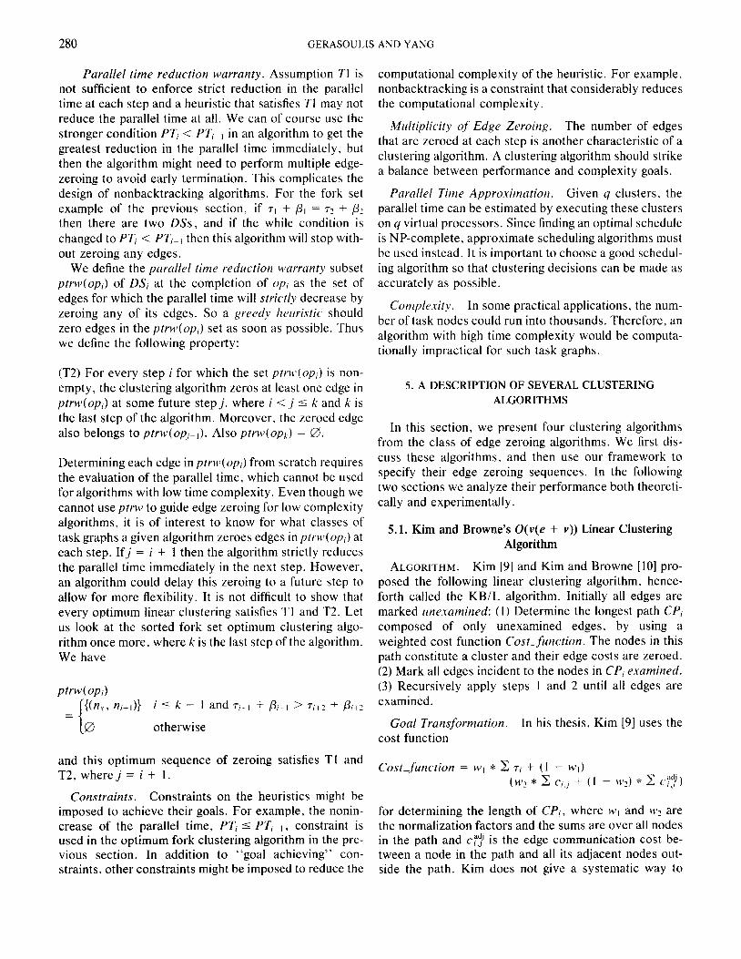
5.1. Kim and Browne’s O(v(e + v)) Linear Clustering Algorithm

ALGORITHM. Kim [9] and Kim and Browne [lo] proposed the following linear clustering algorithm, hence- forth called the KBiL algorithm. Initially all edges are marked unexamined: (1) Determine the longest path CP; composed of only unexamined edges, by using a weighted cost function Cost-function. The nodes in this path constitute a cluster and their edge costs are zeroed. (2) Mark all edges incident to the nodes in CP; examined. (3) Recursively apply steps 1 and 2 until all edges are examined.

Goal Transformation. In his thesis, Kim [9] uses the cost function

Cost-function = M’I * C 3-i + (1 - wi)

for determining the length of CPi, where )+>I and ~‘2 are the normalization factors and the sums are over all nodes in the path and cF.$ is the edge communication cost between a node in the path and all its adjacent nodes out- side the path. Kim does not give a systematic way to

CLUSTERHEURISTICSFORSCHEDULINGDAGS 281

CLU-KEV (KB/L) : Reduce the length of the longest path determined by a cost function.

SCHAZG : No scheduling algorithm is needed since clustering is linear which implies that SG, = G,.

domain(opo) = E.

domain(op,) = E, = E,_, - {e,,h}, n, or nIr E CP,m,.

focus(op.) = Edges in the longest path CP, among all paths in domain(op,).

constraint: Linearity of clustering.

rero(op,) = foc?M(op,). Termination criterion: domain(op,) = 0.

FIG. 6. Edge zeroing operations in KBIL.

determine normalization factors. Here we assume that MJ) = 4 and W? = 1, in which case the cost function reduces to the length of the critical path. Under this assumption Kim’s algorithm can be considered as having the goal of finding the linear clustering with the minimum parallel time (G4/Gl). Each opi for KBiL algorithm is defined in Fig. 6.

EXAMPLE. Consider the example of Fig. la. The result of applying Kim’s linear clustering algorithm is shown in Fig. 1 b with PT = 11.5. The clustering steps are shown in Table I. The symbols (*, n,) and (n, , *) repre- sent the sets of all incoming and outgoing edges of node n, respectively.

At the beginning, the critical path of the original DAG is (n, , ?I?, n7) and these nodes are clustered together. By the deletion of those nodes from the graph, the remaining graph has four nodes (n3, n4, n5, Q). Its critical path is (03, ~4, nb) and these nodes are clustered together. Fi- nally, the resulting clustering is M0 = {n, , II?, n,}, M, = in3 3 124 I n6>, M2 = in&-.

COMPLEXITY. Kim, on page 40 of his thesis, gives the complexity of his Linear-Cluster algorithm as O(u3). The number of connected components is at most u and for each step finding the longest path costs O( u + e). There- fore the complexity of KB/L algorithm is O(u(u + e)). For a dense graph e = u2 and the complexity becomes the upper bound O(u3) given by Kim.

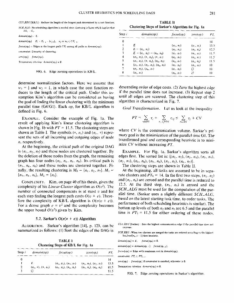
5.2. Sarkar’s O(e( v + e)) Algorithm

ALGORITHM. Sarkar’s algorithm [14], p. 129, can be summarized as follows: (1) Sort the edges of the DAG in

TABLE I Clustering Steps of KB/L for Fig. la

Step i domain(op,) .focus(op,) Txro(op,) PT,

0 14 I E (n,, nd. bZ, n7) (n,. n4. h n7) 13.5 2 (ni, *), (*. 4) h nd. (n4, nd h. rd. h. nJ 11.5 3 !3 11.5

TABLE II Clustering Steps of Sarkar’s Algorithm for Fig. la

Step i dOWlUitl(OpJ focus(op,) zero(op,) PT, --

0 14 I E (n,, 4 (ni, nd 13.5 2 E - (n,, n$ h, n4) Cm. 4) 12.5 3 E - hf. nd - h n4) h. 4) (4, n7) I I.5 4 k71, nil, (*, n& (*, n7) h n7) (n?, n;) I I.5 5 (111~ 4). (*. nJ, h n7) (4. n5) (h n6) II.5 6 (nl, 4). (n5. nd, (n,, n,) h. 4) h t7d IO 7 (nl. 4). (no, ~7) (nl, 4) B I 0 8 (nh. n7) h n7) 0 IO

descending order of edge costs. (2) Zero the highest edge if the parallel time does not increase. (3) Repeat step 2 until all edges are scanned. The clustering step of this algorithm is characterized in Fig. 7.

God Transformation. Let us look at the inequality

PT= C rj+ 11,ED.S

where CV is the communication volume. Sarkar’s primary goal is the minimization of the parallel time G 1. The transformed goal and corresponding heuristic is to minimize CV without increasing PT.

EXAMPLE. For Fig. la, Sarkar’s algorithm sorts all edges first. The sorted list is: {(n,, n2), (n3, n4), (Q, ns). (n2, n7). (a49 n6). (n5, n6), (nl 3 n3)9 (n6, n7)).

The clustering steps are shown in Table II. At the beginning, all tasks are assumed to be in sepa-

rate clusters and PT,, = 14. In the first two steps, (n, , n?) and (n3, n4) are zeroed and the parallel time is reduced to 12.5. At the third step, (n3, ns) is zeroed and the SCH-ALG must be used for the computation of the parallel time. (Sarkar uses a slightly different SCH-ALG, based on the latest starting task time, to order tasks. The performance of both scheduling heuristics is similar). The bottom up levels of both n2 and n3 are 6.5 and the parallel time is PT3 = Il.5 for either ordering of these nodes.

CLUHEU (Sarkar) : Zero the highest communication edge if the parallel time does not increase.

SCHHEU : When two clusters are merged the tasks are ordered according to the highest botJeuel(n,, i - 1) first heuristic.

domain(op,,) = E, focus(opQ) = 0.

domain(op;) = domain(op,-,) - focus(op;_,). focus(op,) = Edge with maximum cost in domain(op,).

constraint: PT. < PT,-l.

rero(op,) = focus(op;) if constraint is satisfied; otherwise is 0.

Termination criterion: domain(op,) = 0.

FIG. 7. Edge zeroing operations in Sarkar’s algorithm.


Then at step 4, (nz, 1~) is zeroed, and the parallel time remains the same PTd = I I .5. In the following steps, (~24, nb), ( kzs, QJ are zeroed and PTd reduces to 10. The edges (n, , nj) and (rzh, n,) cannot be zeroed: otherwise all nodes would be in the same cluster and the parallel time would increase to 13. Finally, Sarkar’s algorithm obtains two clusters with PT = 10. as shown in Fig. 1 lb: M. = {ni , n2, n7), Ml = {n3, 124, ns , n$-.

As it can be seen from the goal transformation inequality, minimizing CV may not reduce the parallel time at all, unless the corresponding zeroed edges belong to DS. For example. in the fourth step above, the dominant sequence is (n, , I?~, 12~. tr5, 12~. n,). However, Sarkar’s algorithm is unable to identify this sequence. It zeros the edge h 2 tz,) which is not in this DS and the parallel time remains unchanged. Had the edge tn6, n7) been zeroed instead, the parallel time would have been reduced to 9.

Complexity. Sarkar computes the levels at each clustering step, and then uses the level information to schedule the tasks and to determine the parallel time. The computation of the levels costs O(u + e) at each step and since there are c such steps the total cost of the algorithm is at least O(e(u + E)).

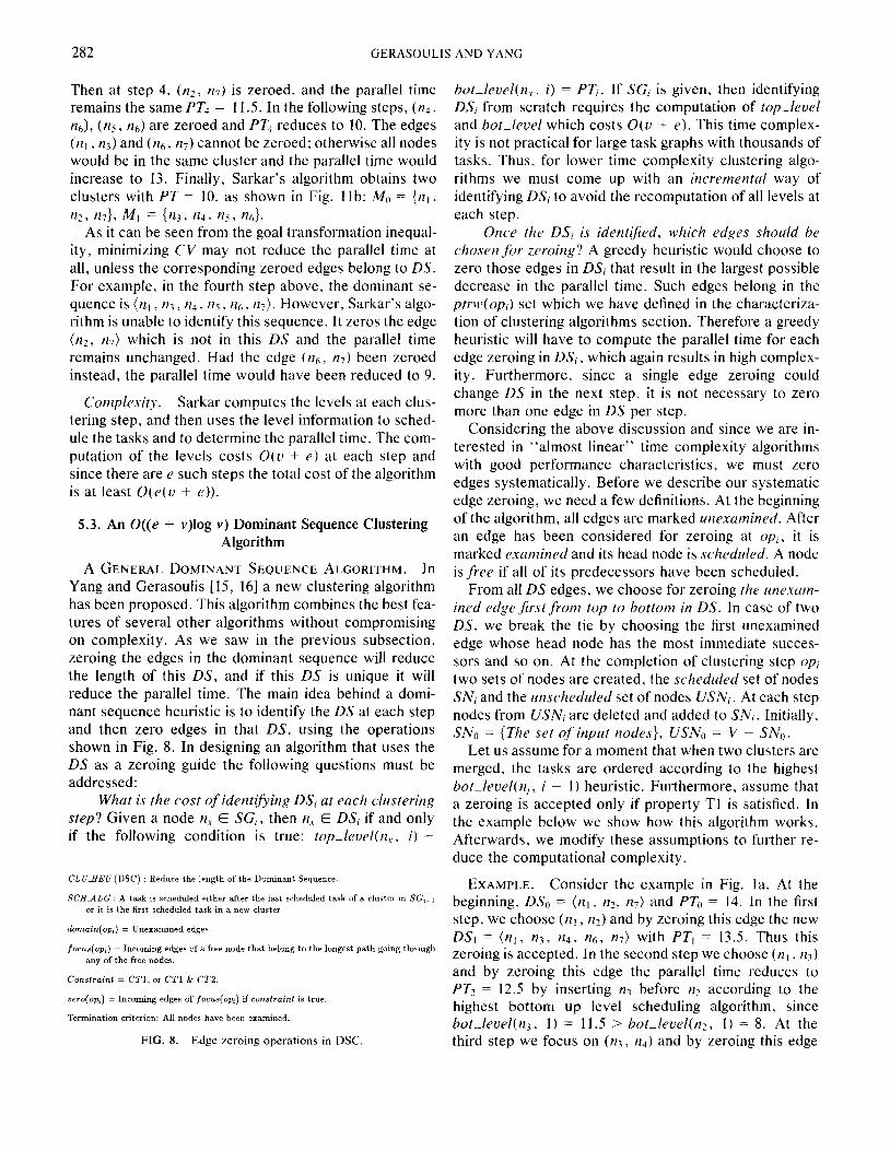
5.3. An O((e + v)log v) Dominant Sequence Clustering Algorithm

A GENERAL DOMINANT SEQUENCE ALGORITHM. In Yang and Gerasoulis [15, 161 a new clustering algorithm has been proposed. This algorithm combines the best features of several other algorithms without compromising on complexity. As we saw in the previous subsection, zeroing the edges in the dominant sequence will reduce the length of this DS, and if this DS is unique it will reduce the parallel time. The main idea behind a dominant sequence heuristic is to identify the DS at each step and then zero edges in that DS. using the operations shown in Fig. 8. In designing an algorithm that uses the DS as a zeroing guide the following questions must be addressed:

What is the cost of identij>ing DSi at each clustering step? Given a node II, E SGi. then IZ., E DS, if and only if the following condition is true: top-leve/(n,, i) +

CLUHEU (DSC) : Reduce the length of the Dominant Sequence.

SCHALG : A task 1s scheduled either after the last scheduled task of a cluster in SG,-1 or it is the first scheduled task in a new cluster.

domain(op,) = Unexamined edges.

focus(op;) = Incoming edges of a free node that belong to the longest path going through any of the free nodes.

Constraint = CTl, or CT1 & CT2.

zero(op,) = Incoming edges of focus(op;) if constraint is true.

Termination criterion: All nodes have been examined.

FIG. 8. Edge zeroing operations in DSC.

hot-leuel(n,. , i) = PT,. If SGi is given, then identifying DS; from scratch requires the computation of top-feuel and bot-leuel which costs O(u + e). This time complexity is not practical for large task graphs with thousands of tasks. Thus, for lower time complexity clustering algorithms we must come up with an incremental way of identifying DSi to avoid the recomputation of all levels at each step.

Once the DSi is ident$ed. which edges should be choserlfi)r zeroing? A greedy heuristic would choose to zero those edges in DS; that result in the largest possible decrease in the parallel time. Such edges belong in the ptrw(op;) set which we have defined in the characterization of clustering algorithms section. Therefore a greedy heuristic will have to compute the parallel time for each edge zeroing in DS;, which again results in high complexity. Furthermore, since a single edge zeroing could change DS in the next step, it is not necessary to zero more than one edge in DS per step.

Considering the above discussion and since we are in- terested in “almost linear” time complexity algorithms with good performance characteristics, we must zero edges systematically. Before we describe our systematic edge zeroing, we need a few definitions. At the beginning of the algorithm, all edges are marked unexamined. After an edge has been considered for zeroing at opi, it is marked examined and its head node is scheduled. A node is free if all of its predecessors have been scheduled.

From all DS edges, we choose for zeroing the unexamined edge first from top to bottom in DS. In case of two DS, we break the tie by choosing the first unexamined edge whose head node has the most immediate successors and so on. At the completion of clustering step <pi two sets of nodes are created, the scheduled set of nodes SN, and the unscheduled set of nodes USN,. At each step nodes from USN, are deleted and added to SN;. Initially, SN” = (The set of input nodes}, USNO = V - SN,,.

Let us assume for a moment that when two clusters are merged, the tasks are ordered according to the highest hot-leuel(n,, i - 1) heuristic. Furthermore, assume that a zeroing is accepted only if property TI is satisfied. In the example below we show how this algorithm works. Afterwards, we modify these assumptions to further reduce the computational complexity.

EXAMPLE. Consider the example in Fig. la. At the beginning, DS,, = (n, , n?, n,) and PTo = 14. In the first step, we choose (n, , nz) and by zeroing this edge the new DSI = (nl, n3. n4, n6, n-i) with PT, = 13.5. Thus this zeroing is accepted. In the second step we choose (n, , n3) and by zeroing this edge the parallel time reduces to PTz = 12.5 by inserting n3 before 12~ according to the highest bottom up level scheduling algorithm, since botAeuel(n3, I) = 11.5 > hot-leue/(n?, I) = 8. At the third step we focus on (nj, 1z4) and by zeroing this edge

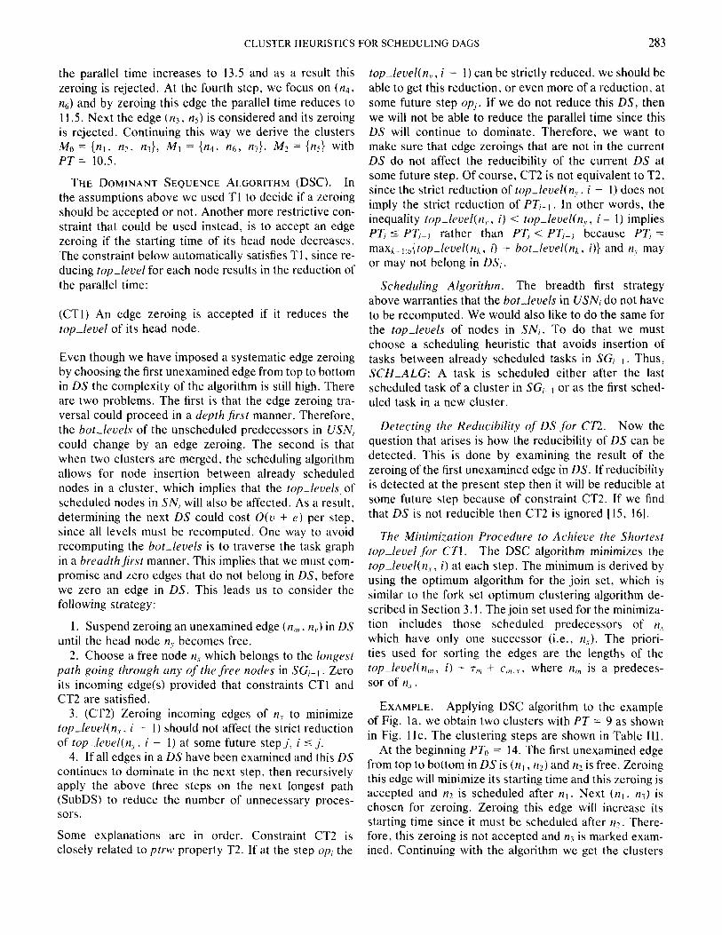
CLUSTER HEURISTlCS FOR SCHEDULING DAGS 283

the parallel time increases to 13.5 and as a result this zeroing is rejected. At the fourth step, we focus on (n4, Q) and by zeroing this edge the parallel time reduces to 11 S. Next the edge (Q, ttS) is considered and its zeroing is rejected. Continuing this way we derive the clusters MO = {n, , nz, nj}, MI = (4, 4, no}, Mz = {ns} with PT = 10.5.

THE DOMINANT SEQUENCE ALGORITHM (DSC). In the assumptions above we used Tl to decide if a zeroing should be accepted or not. Another more restrictive constraint that could be used instead, is to accept an edge zeroing if the starting time of its head node decreases. The constraint below automatically satisfies T 1, since reducing top-level for each node results in the reduction of the parallel time:

(CTl) An edge zeroing is accepted if it reduces the top-.level of its head node.

Even though we have imposed a systematic edge zeroing by choosing the first unexamined edge from top to bottom in LX the complexity of the algorithm is still high. There are two problems. The first is that the edge zeroing traversal could proceed in a depth jirst manner. Therefore, the bot-levels of the unscheduled predecessors in USN, could change by an edge zeroing. The second is that when two clusters are merged, the scheduling algorithm allows for node insertion between already scheduled nodes in a cluster, which implies that the top-levels of scheduled nodes in SN; will also be affected. As a result, determining the next DS could cost O(v + e) per step, since all levels must be recomputed. One way to avoid recomputing the hot-levels is to traverse the task graph in a breadth-first manner. This implies that we must com- promise and zero edges that do not belong in DS, before we zero an edge in DS. This leads us to consider the following strategy:

1. Suspend zeroing an unexamined edge (n,>!. fz,.) in DS until the head node n? becomes free.

2. Choose a free node n, which belongs to the longest path going through my of the free nodes in SGi-, , Zero its incoming edge(s) provided that constraints CT1 and CT2 are satisfied.

3. (CT2) Zeroing incoming edges of n, to minimize top-fevel(n., , i - 1) should not affect the strict reduction of top-level(n, , i - 1) at some future step j, i 5 j.

4. If all edges in a DS have been examined and this DS continues to dominate in the next step, then recursively apply the above three steps on the next longest path (SubDS) to reduce the number of unnecessary processors.

Some explanations are in order. Constraint CT2 is closely related to ptrw property T2. If at the step op, the

top-level(n,, i - 1) can be strictly reduced, we should be able to get this reduction, or even more of a reduction, at some future step opj. If we do not reduce this DS, then we will not be able to reduce the parallel time since this DS will continue to dominate. Therefore, we want to make sure that edge zeroings that are not in the current DS do not affect the reducibility of the current DS at some future step. Of course, CT2 is not equivalent to T2, since the strict reduction of top-level(n,, i - 1) does not imply the strict reduction of PTi-1. In other words, the inequality top-leuel(n,., i) < top-leuel(n,,, i- 1) implies PT, 5 PTjmr rather than PT, < PTi-] because PT, = maxk,l:,{top-level(nk, i) + bot-level(nk, i)} and n, may or may not belong in LX;.

Scheduling Algorithm. The breadth first strategy above warranties that the bot-levels in USNi do not have to be recomputed. We would also like to do the same for the top-levels of nodes in SN,. To do that we must choose a scheduling heuristic that avoids insertion of tasks between already scheduled tasks in SG;-i . Thus, SCH-ALG: A task is scheduled either after the last scheduled task of a cluster in SG;-i or as the first scheduled task in a new cluster.

Detecting the Reducibility of DS for CT2. Now the question that arises is how the reducibility of DS can be detected. This is done by examining the result of the zeroing of the first unexamined edge in DS. If reducibility is detected at the present step then it will be reducible at some future step because of constraint CT2. If we find that DS is not reducible then CT2 is ignored [ 15, 161.

The Minimization Procedure to Achieve the Shortest top-leuel for CTl. The DSC algorithm minimizes the top-level(n,, i) at each step. The minimum is derived by using the optimum algorithm for the join set, which is similar to the fork set optimum clustering algorithm described in Section 3.1. The join set used for the minimization includes those scheduled predecessors of ?I, which have only one successor (i.e., II,). The priorities used for sorting the edges are the lengths of the top-level(n,,,, i) + T,,, + c ,,,.., , where n,, is a predecessor of n, .

EXAMPLE. Applying DSC algorithm to the example of Fig. la, we obtain two clusters with PT = 9 as shown in Fig. 1 lc. The clustering steps are shown in Table III.

At the beginning PT,, = 14. The first unexamined edge from top to bottom in DS is (n, ,[I?) and n2 is free. Zeroing this edge will minimize its starting time and this zeroing is accepted and nz is scheduled after nl . Next (n,, Q) is chosen for zeroing. Zeroing this edge will increase its starting time since it must be scheduled after 11~. There- fore, this zeroing is not accepted and n3 is marked examined. Continuing with the algorithm we get the clusters

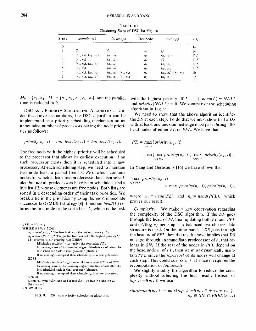
284 GERASOULlS AND YANG

TABLE III Clustering Steps of DSC for Fig. la

Step i

0 1 0 2 MI, n2). (n,, nz) 3 (nt, n3) 4 (ni, nd. h n4 5 (4 n5) 6 h, 4). (4. n6) 7 h, n7). (n,, n7)

free node :ero(up,) PT,

14 0 14 (n,. 124 13.5 0 13.5 (ni. n4) 12.5 (n3. I14 Il.5 h. n6). (nc. n6) IO

h. n7) 9

MO = 02, , &>, M, = (113, n 4, ns , nh, n-i}. and the parallel time is reduced to 9.

DSC AS A PRIORITY SCHEDULING ALGORITHM. Un- der the above assumptions, the DSC algorithm can be implemented as a priority scheduling mechanism on an unbounded number of processors having the node priorities as follows:

priority(nl;, i) = top-level(nk, i) + hot-level(nk, i).

The free node with the highest priority will be scheduled to the processor that allows its earliest execution. If no such processor exists then it is scheduled into a new processor. At each scheduling step, we need to maintain two node lists: a partial free list PFL which contains nodes for which at least one predecessor has been scheduled but not all predecessors have been scheduled, and a free list FL whose elements are free nodes. Both lists are sorted in a descending order of their task priorities. We break a tie in the priorities by using the most immediate successor first (MISF) strategy [8]. Function head(L) re- turns the first node in the sorted list L, which is the task

USN,, = V; i = 0 WHILE USN; # 0 DO

nz = head(FL The free task with the highest priority. * / n, = head(PFL); /* The partial free task with the highest priority.*/ IF (priority(n,) 2 piority(n,)) THEN

Minimize topJevel(n,, i) under the constraint CT1 by zeroing some of its incoming edges. Schedule a task after the last scheduled task in that processor (cluster). If no zeroing is accepted then schedule n, in a new processor.

ELSE Minimize topJevel(n,, i) under the constraint CT1 and CT2 by zeroing some of its incoming edges. Schedule a task after the last scheduled task in that processor (cluster). If no zeroing is accepted then schedule n, in a new processor.

ENDIF Delete nz from USN, and add it into SN;. Update FL and PFL. set i = it 1.

ENDWHILE

FIG. 9. DSC as a priority scheduling algorithm.

with the highest priority. If L = { }, head(L) = NULL and priority(NULL) = 0. We summarize the scheduling algorithm in Fig. 9.

We need to show that the above algorithm identifies the DS at each step. To do that we must show that a DS with at least one unexamined edge must pass through the head nodes of either FL or PFL. We have that

PT; = max{priority(n,, i)} y=l:l:

= max{max priority(n,, i), max priority(n,, i)}. n,t SN, n,E USN,

In Yang and Gerasoulis [16] we have shown that

max priority( nq , i) n,,t USN,

= max{priority(n,, i), priority(n,. , i)},

where n, = head and nY = head(PFL), which proves our result.

Complexity. We make a key observation regarding the complexity of the DSC algorithm. If the DS goes through the head of FL then updating both FL and PFL costs O(log v) per step if a balanced search tree data structure is used. On the other hand, if DS goes through the head n? of PFL then the result above implies that DS must go through an immediate predecessor of n, that belongs in SN;. If the rest of the nodes in PFL depend on the head node n.,. of FL, then we must dynamically maintain PFL since the top-level of its nodes will change at each step. This could cost O(v + e) since it requires the recomputation of top-leuels.

We slightly modify the algorithm to reduce the complexity without affecting the final result. Instead of top-level(nk, i) we use

startbound(nr, i) = max{top-level(n,,. i) + T,,, + c,),.~}. n,, E SN, rl PRED(nk , i)


CLUHEU (MCP) : Tasks with the highest priority in the critical path should start execution at the earliest possible time.

SCHALG : A task is scheduled either after the last scheduled task of a cluster in SG,-1 or it is the lint scheduled task in a new cluster.

domain(op;) = Unexamined edges.

focus(op.) = Incoming edge of a free node with the highest priority.

constraint = CTl.

rero(op;) = Incoming edge in focus(op,) if constraint is true.

Termination criterion: All nodes have been scheduled

FIG. 10. Edge zeroing operations in MCP

where PRED(nk, i) is the set of immediate scheduled predecessors of nk in SG;. We can easily show that startbound is a lower bound of top-level, see Yang and Gera- soulis [16], by proving

startbound(nk , i) 5 top-level(nk , i), n!, E PFL, startbound(n,, i) = top-level(n,, i), n, = head(PFL), startbound(nk, i) = top-level(nk, i), n!. E FL.

Maintaining FL and PFL priority lists cost O(log v) and since there are v steps the cost is O(v log v). Adding the graph traversal cost of O(u + e) for a total O(v log u + e).

The incoming edge zeroing minimization procedure can be computed in O(l PRED(n,)llogl PRED(n,)l) which is the cost for sorting the priorities of its predecessors. Summing over all tasks we get an upper bound estimate of O(e log v). Thus the total time complexity of DSC is O((u + e)log u). The space complexity is O(v + e). For linear clustering the cost reduces to O(v log u + e).

5.4. Wu and Gajski’s MCP O(v2 log v) Clustering Algorithm

This implies that minimizing the starting time of the last task could result in the reduction of the overall parallel time. Therefore the transformed goal is the minimization of the starting time of the output task. The MCP heuristic is trying to achieve this by starting the execution of every ‘,ask at the earliest possible time. Since ST(n,) = top-level(n,, i), then reducing the starting time for each task implies PTi 2 PTi- i and this algorithm satisfies Tl. The algorithm does not satisfy T2 for a general DAG.

ALGORITHM. Wu and Gajski [17] have proposed two scheduling algorithms for a bounded number of processors. These are the MCP (Modified Critical Path) and MD (Mobility Directed). The MCP reduces to an edge-zeroing clustering algorithm when it is used as a scheduling algorithm on a completely connected architecture with unbounded number of processors. On the other hand, the MD algorithm is not an edge-zeroing algorithm and we will not compare it with the other algorithms in this paper.

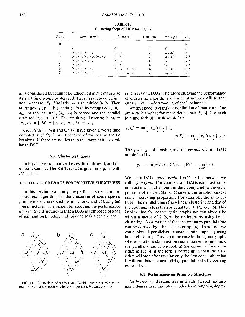
EXAMPLE. We apply this algorithm on the task graph in Figure l(a). The final clustering is shown in Fig. 1 la. The stepwise result is shown in Table IV.

Initially, the tasks are mapped in separate clusters and the priorities are computed. The following priority list, along with the priority tuples, which include the bottom up level, the highest bottom up level of its child, and so on, iseasilyderived: {n, (14, 115.8, . . . . l), n1(11.5, 6.5, . . . ) I), nz (8, l), n4 (6.5, 3, 1). ns (6.5, 3. I), Q, (3, l), 117 (1)).

The MCP algorithm is described below: First 12~ is scheduled to processor PO. At the second

step, the free task n3 is selected and is scheduled to PO since its starting time reduces from 2 to 1. At the third step, rzz is scheduled in PO after 12~ according to SCH-ALG, since again this processor allows its earliest execution. Now the parallel time becomes PT7 = 12.5 which is the length of the DS = (n, , n3, n4. nh. n,). Next

Determine a priority list based on the “highest bot-level first” ordering of SGO. If two tasks have the same level then break the tie by using the highest level of its successor tasks, the successor of its successors and so on.

WHILE (There exists an unscheduled task) DO Find an unscheduled free node with the highest

priority in the priority list. Schedule this task to a processor (cluster) that

allows its earliest execution. ENDWHILE

There are certain similarities between the DSC and the MCP algorithm. They are both implemented as scheduling algorithms that have the earliest starting time heuristic as a scheduling guide. There is however a major differ- ence in the choice of the priorities in the free list. The DSC uses the sum of top-level and hot-level of SG; while the MCP uses only the hot-leuel of SGo. As a result the MCP cannot identify the dominant sequence and may not zero its edges. The view of the MCP algorithm as an edge-zeroing algorithm is given in Fig. 10.

Goal Transformation. The primary goal for this algorithm is Gl, the minimization of the parallel time. The cost function for GI is the parallel time which is equal to

PT = max(ST(nj) + Tj) 5 max ST(n;) + max 7i. .i i i

286 GERASOULIS AND YANG

TABLE IV Clustering Steps of MCP for Fig. la

Step i free node xro(op,J PT,

0 1 0 0 2 O?l, nz), (n,. n7J (n,, nd 3 (~ZI, 4. h nd, h. n<l (n,. 112) 4 h, nd. (9. 4 h, t2d 5 (n3, 4) h, nd 6 (4, 4). h. 4) h. 4). (4. 4 7 (n2. n7), (n,. n,J h n7). (4. n,)

14 nl 0 14 n, (fll, ?I 14 ,,I 011, t1d 12.5 n4 63 12.5 II5 0 12.5 4 (n4, nd Il.5 n7 (n6, n7) 10.5

124 is considered but cannot be scheduled in PO ; otherwise its start time would be delayed. Thus n4 is scheduled in a new processor Pi. Similarly, n5 is scheduled in P?. Then at the next step, n6 is scheduled in P, by zeroing edge (n4, nJ. At the last step, (n6, n,) is zeroed and the parallel time reduces to 10.5. The resulting clustering is MO = {nk, 4, nd, MI = (124, n6, n71, M7 = (4.

Complexity. Wu and Gajski have given a worst time complexity of O(u? log u) because of the cost in the tie breaking. If there are no ties then the complexity is similar to DSC.

5.5. Clustering Figures

In Fig. 11 we summarize the results of three algorithms on our example. The KB/L result is given in Fig. lb with PT = 11.5.

6. OPTIMALITY RESULTS FOR PRIMITIVE STRUCTURES

In this section, we study the performance of the previous four algorithms in the clustering of some special primitive structures such as join, fork, and coarse grain tree structures. The reason for studying the performance on primitive structures is that a DAG is composed of a set of join and fork nodes, and join and fork trees are span-

FIG. 11. Clusterings of (a) Wu and Gajski’s algorithm with PT = 10.5: (b) Sarkar’s algorithm with PT = IO: (c) DSC with PT = 9.

ning trees of a DAG. Therefore studying the performance of clustering algorithms on such structures will further enhance our understanding of their behavior.

We first need to clarify our definition of coarse and fine grain task graphs; for more details see [S, 61. For each join and fork of a task we define

h= I:m k=l:nr g(F,) = min {rk}/max {c.~J,}.

h= I:m h=l~,,r

The grain. gl, of a task n., and the granularity of a DAG are defined by

g, = minkdt;,), g(J,)), g(G) = min kc>. tl,Eb’

We call a DAG coarse grain if s(G) Z- 1, otherwise we call it fine grain. For coarse grain DAGs each task com- municates a small amount of data compared to the computation of its neighbors. Coarse grain graphs possess many interesting properties. For example, the ratio between the parallel time of any linear clustering and that of the optimum is less than or equal to 1 + l/g(G), [6]. This implies that for coarse grain graphs we can always be within a factor of 2 from the optimum by using linear clustering. As a matter of fact the optimum parallel time can be derived by a linear clustering, [6]. Therefore, we can exploit all parallelism in coarse grain graphs by using linear clustering. This is not the case for fine grain graphs where parallel tasks must be sequentialized to minimize the parallel time. If we look at the optimum fork algorithm in Fig. 4, if the fork is coarse grain then the algorithm will stop after zeroing only the first edge; otherwise it will continue sequentializing parallel tasks by zeroing more edges.

6.1. Performance on Primitive Structures

An in-tree is a directed tree in which the root has outgoing degree zero and other nodes have outgoing degree


TABLE V Performance of Clustering Algorithms on Primitive Structures

Join Fork In-tree Out-tree

T? Opt. T7 Opt. T? Opt. T2 opt.

Coarse grain KBIL Yes Yes Yes Yes Yes No Yes No Sarkar No No No No No No No No DSC Yes Yes Yes Yes Yes Yes Yes No MCP Yes Yes No No Yes Yes No No

Fine grain KBiL No No No No No No No No Sarkar No No No No No No No No DSC Yes Yes Yes Yes Yes No Yes No MCP No No No No No No No No

one. An out-tree is a directed tree in which the root has incoming degree zero and other nodes have incoming degree one. A join is an in-tree of depth 1. Afovli is an out- tree of depth 1.

All algorithms satisfy property Tl, the monotonic reduction in the parallel time. For other performance features, Table V summarizes the comparative results on the primitive structures.

We now provide the proof for the above performance results.

6.1.1. Performance on Fork and Join

PROPOSITION 6.1.1 (DSC Algorithm). For the fork and join graphs thr DSC algorithm derives the optimum clustering and also satisJies property T2.

Proof. For both join and fork, the DSC algorithm derives the same edge zeroing sequence as the optimal algorithm in Section 3.1 which satisfies Tl and T2, as shown in Section 4. n

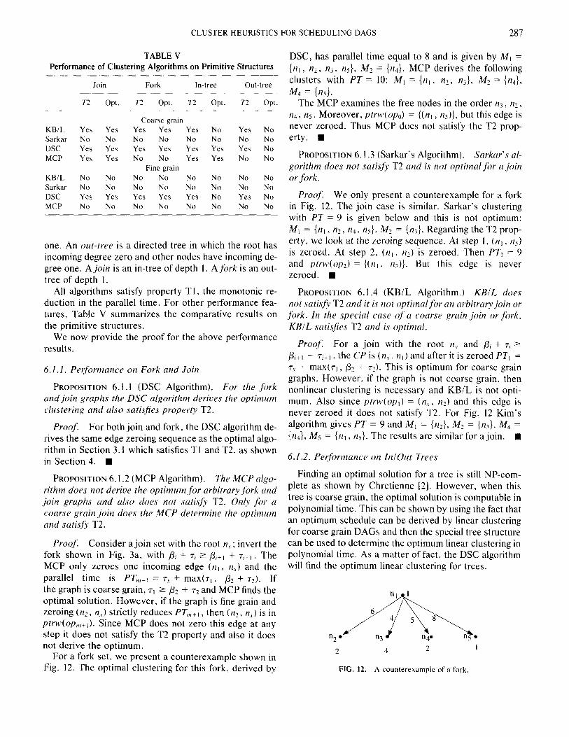
PROPOSITION 6. I .2 (MCP Algorithm). The MCP ulgo- rithm does not derive the optimum for arbitrary fork and join graphs and also does not sati& T2. Only for a coarse grain join does the MCP determine the optimum and satisfy T2.

Proof. Consider a join set with the root n.,; invert the fork shown in Fig. 3a, with pi + T, 2 pi+, + T;+, . The MCP only zeroes one incoming edge (n, , n,) and the parallel time is PT,,,, = T.~ + max(T,, pZ + TV). If the graph is coarse grain, 7, 2 p1 + 7? and MCP finds the optimal solution. However, if the graph is fine grain and zeroing (nz, 12,) strictly reduces PT,,]+, , then (nz, n,) is in ptrw(op,,,+,). Since MCP does not zero this edge at any step it does not satisfy the T2 property and also it does not derive the optimum.

For a fork set, we present a counterexample shown in Fig. 12. The optimal clustering for this fork, derived by

DSC, has parallel time equal to 8 and is given by M, = InI, n2, n3. IQ}, Mz = {n4}. MCP derives the following clusters with PT = 10: M, = {n, , n!, n3}, Mz = {n4}, M4 = ins).

The MCP examines the free nodes in the order n3, IQ, n4, n5. Moreover, ptni>(op”) = ((0, , ns)}, but this edge is never zeroed. Thus MCP does not satisfy the T2 property. n

PROPOSITION 6.1.3 (Sarkar’s Algorithm). Sarkar’s algorithm does not satisfy T2 and is not optimal for a join or fork.

Proof. We only present a counterexample for a fork in Fig. 12. The join case is similar. Sarkar’s clustering with PT = 9 is given below and this is not optimum: M, = {n, , nz, n4, IIS}, M2 = {II-(}. Regarding the T2 property, we look at the zeroing sequence. At step I, (/I,, n) is zeroed. At step 2, (n,, n2) is zeroed. Then PT? = 9 and ptrw(op,) = {(n, , nd}. But this edge is never zeroed. n

PROPOSITION 6.1.4 (KBIL Algorithm.) KBiL does not satisfv T2 and it is not optimal for an arbitrary join or fork. In the special case of a coarse grain join or fork, KBIL satisfies T2 and is optimal.

Proof. For a join with the root n, and pi + ~~ 2 pi+, + 7;+, , the CP is (~2~. n,) and after it is zeroed PT, = T., + maX(Tl, pz + T?). This is optimum for coarse grain graphs. However, if the graph is not coarse grain, then nonlinear clustering is necessary and KBiL is not optimum. Also since ptrwl(op,) = ()I,, n,) and this edge is never zeroed it does not satisfy T2. For Fig. 12 Kim’s algorithm gives PT = 9 and M, = {nz}, MZ = {n-i}, M4 = {nd}, Mc = {n, , n5}. The results are similar for a join. l

6.1.2. Performance on inlOut Trees

Finding an optimal solution for a tree is still NP-complete as shown by Chretienne [2]. However, when this tree is coarse grain, the optimal solution is computable in polynomial time. This can be shown by using the fact that an optimum schedule can be derived by linear clustering for coarse grain DAGs and then the special tree structure can be used to determine the optimum linear clustering in polynomial time. As a matter of fact, the DSC algorithm will find the optimum linear clustering for trees.

%.A.. 2 4 2 I

FIG. 12. A counterexample of a fork


PROPOSITION 6.1.5 (DSC Algorithm). DSC satisfies T2 and gives the optimal solution for coarse grain in- trees but not for fine grain in-trees. For both fine and coarse grain out-trees, DSC satisfies T2 but it is not optimal.

Proof. The optimum solution can be derived by DSC for coarse grain in-trees. It is proven by induction on the depth of the tree in Yang and Gerasoulis [15, 161 by showing that DSC produces a schedule where every node has the minimum starting time.

nlo 2 n2 . 2

2

v

0.5

“‘L 7’

\/ ng.4

FIG. 13. A counterexample of an in-tree.

Without inverting an out-tree, DSC cannot get the optimum but it still satisfies the T2 property. We prove it in two steps.

In the first step we show that ifptrw(op;) # 0, then the edges in ptrw(opi) must be unexamined. If not, suppose (n,, n,) E ptrw(op;) and it has been examined and n1 has been scheduled. Zeroing (n,, , n,) will strictly reduce the parallel time implying that the starting time n, can be reduced. Since n, has only one incoming edge (rzY, n,), if the assumption were true, (n, n,) would have been zeroed when nt was scheduled, a contradiction.

Next we must prove that (n,, n,) will be zeroed at some future step. Assume that the topmost unexamined edge in the current DS, and which also belongs to ptrw(opi), is 0% 1 n,). From step i + 1 to the step when n, becomes free, the parallel time cannot be reduced and ()I,~, n,) is always in the ptrw set. At the step at which n, becomes free, it must have the highest priority and then (n,, , n,) must be zeroed to reduce the starting time of n,. H

PROPOSITION 6.1.6 (MCP Algorithm). MCP satisjes

DS; = CPi since KB/L is a linear clustering algorithm. Now assume that (n, n,) E ptrw(op;). This means that the parallel time is reducible by zeroing this edge. We first show that no incoming edge of n, has been examined or zeroed at any step less or equal to i. Assume the con- trary, which means that one incoming edge has been zeroed and the others, including (n,, , n,), have been examined. Then zeroing (n,, n,) is impossible to reduce the parallel time because the tree is coarse grain. That is a contradiction. Secondly, since KB/L zeroes all edges in the CP of each subgraph at each step and the subgraph is a subtree, we can easily see that all edges in the subtree rooted with n, are not examined. As a result, when the global CP of the whole tree (called GCP) goes through any unexamined subtree, the part of GCP in this subtree is also the CP of this subtree. And when KB/L is working on the subtree where (n, , n,) resides, the edges in its CP including (n, n,) will be zeroed.

T2 and gives the optimal solution for coarse grain in- trees but not for general in-trees. For out-trees, MCP does not satisfy T2 and it is not optimal.

Proof. Since the problem itself is NP-complete, for general in-trees and out-trees the MCP cannot determine the optimum. Also since for the special case of fork/join MCP does not satisfy T2, it does not satisfy T2 in general.

The proof that for a coarse grain in-tree, MCP is optimal and satisfies T2 is similar to DSC. When the tree has height 1 and is a coarse grain join then MCP determines the optimum. Inductively, we can prove that it determines the optimum for coarse grain in-trees. n

PROPOSITION 6.1.7 (KBIL Algorithm). KBIL is not optimalfor any tree and in general does not sati& T2. It only satisfies T2 for coarse-grain inlout-trees.

Next, we show that one such edge (rzY, n,) is still in ptrw when that edge is zeroed. If KB/L does not zero any edge in ptrw(opi) after step i until stepj, then no edge in GCP is zeroed during those steps and ptrw does not change. If this is not true, assume that (n, , n?) is an edge in GCP but not in ptrw which is zeroed in step k such that i < k < j. Now since (n, n,) is also in the GCP, the edge (nl , n2) must lie either on the root side of (n, , n,) or on the leaf side. If (nl , n2) lies on the leaf side of (n, n,), all the edges in the CP of the subtree including (n,, , n,) will be zeroed in step k which is a contradiction. If on the other hand, (n,, nz) lies on the root side of (n,, 1~) then it should also be in ptrw(opi) which is again a contradiction. n

PROPOSITION 6.1.8 (Sarkar’s Algorithm). Sarkar’s algorithm does not satisfy T2 and is not optimal for a tree.

Proof. The simplest counterexample is a fork (or join), where Sarkar’s does not satisfy T2 and is not optimal in general. n

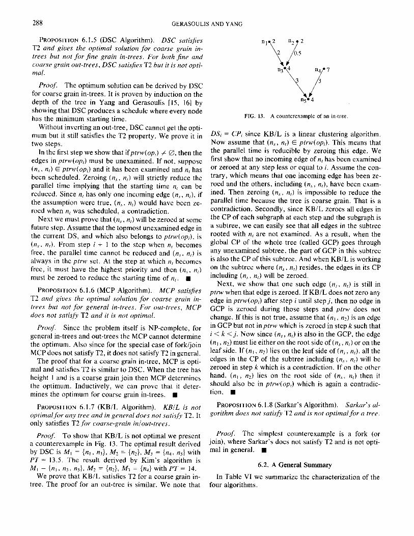
Proof. To show that KB/L is not optimal we present a counterexample in Fig. 13. The optimal result derived by DSC is MI = {n,, n3}, MZ = {nz}, M3 = {n4, ns} with PT = 13.5. The result derived by Kim’s algorithm is MI = {n, , n3. ns}, MZ = {nz}. Mj = {nd} with PT = 14.

We prove that KB/L satisfies T2 for a coarse grain in- tree. The proof for an out-tree is similar. We note that four algorithms.

6.2. A General Summary

In Table VI we summarize the characterization of the

CLUSTER HEURISTICS FOR SCHEDULING DAGS

TABLE VI A Comparison of Four Clustering Algorithms

289

Sarkar MCP KBiL DSC

Goals Transformed goals

Multiplicity of zeroing Constraint imposed Tl T2

Complexity

Gl Reduce

cv One Tl Yes No

e(u + e)

GllG2

Minimize starting time One Nonincrease in ST Yes No

d log v

G4IG 1

Compress CP in subgraphs All in CP Linearity of clustering Yes No

v(v + f)

GIIG2

Compress DS Some incoming edges of a free node CTI, or CTI and CT2 Yes No for fine grain Yes for coarse grain (e + LJ) log u

Note that DSC satisfies T2 for any coarse grain DAG. The proof is similar to the one given for the out-tree case. The coarse grain constraint ensures that only one incoming edge would be zeroed if it would be zeroed.

7. EXPERIMENTAL RESULTS AND COMPARISONS

DSC vs. SARKAR'S. In Yang and Gerasoulis [15] we compared the DSC algorithm and Sarkar’s algorithm on 100 randomly generated DAGs and weights. These graphs are produced by randomly generating the number of tasks and edges and assigning random numbers as weights. The size of the graphs varies from a minimum of 70 nodes with 311 edges to a maximum of 329 nodes with 3430 edges. The ratio of computation and communication varies from 0.8 to 8.7. On the average we found that PTDsc = .83 PTSarkar for these graphs. As far as the algorithm execution speed is concerned, DSC is one order faster than Sarkar’s.

DSC vs. OTHER CLUSTERING HEURISTICS. We have chosen for experimentation the well-known Cholesky Decomposition (CD) DAG. There are several reasons for choosing this DAG for comparison. One is that we can compute the clustering of KB/L analytically rather than computationally which will be impossible because of the high complexity. Another reason is that we would like to compare DSC with the natural clustering which is a widely used clustering for this DAG [4, 121. However, we did not include Sarkar’s heuristic because the graph is too large to be handled.

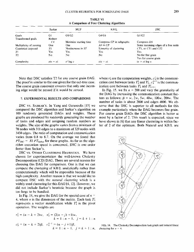
In Fig. 14, we give the DAG for the special case of n = 4, where n is the dimension of the matrix. Each task T$ represents a vector modification while T:’ is the pivot operation. The weights are

r: = (n - k + 2)w, ri = (2(n - j) + l)w, k=l:n-1, j=k+l:n

c$ = (n - k + 2)& cf+’ = (n - j +I)& k=l:n-1, j=k+l:n,

where 7i are the computation weights, c$ is the communication cost between tasks Tf and T$, cf+’ is the communication cost between tasks Ti and T$+, .

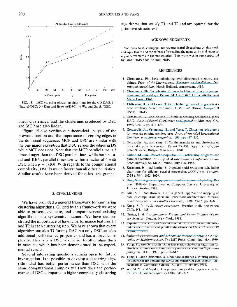
In Fig. 15, we fix n = 200 and vary the granularity of the DAG by increasing the communication constant factors as follows; p = w, 2w, SW, 4Ow, lOOw, 200~. The number of tasks is about 2000 and edges 4000. We ob- serve that the DSC is superior to all methods for this example particularly when the DAG becomes fine grain. For coarse grain DAGs the DSC algorithm is better at most by a factor of 2. This result is expected, since we have shown in [6] that any linear clustering is within factor of 2 of the optimum. Both Natural and KBlL are

FIG. 14. The Cholesky Decomposition task graph and natural linear clustering for n = 4.


PT Speedup Ratio for CD.n=200

<-coax grain lk Fine grain->

FIG. 15. DSC vs. other clustering algorithms for the CD DAG: (+) Natural/D%: (*) Kim and BrowneiDSC: (0) Wu and GajskiiDSC.

linear clusterings, and the clusterings produced by DSC and MCP are also linear.

Figure 1.5 also verifies our theoretical analysis of the previous section and the importance of zeroing edges in the dominant sequence. MCP and DSC are similar with the one major exception that DSC zeroes the edges in DS while MCP does not. Note that the MCP parallel time is 3 times longer than the DSC parallel time, while both natural and KB/L parallel times are within a factor of 4 with DSC when g = l/200. With regards to the computational complexity, DSC is much faster than all other heuristics. Similar results have been derived for other task graphs.

8. CONCLUSIONS 10.

We have provided a general framework for comparing clustering algorithms. Guided by this framework we were able to present, evaluate, and compare several existing algorithms in a systematic manner. We have demonstrated the importance of having performance features Tl and T2 in each clustering step. We have shown that every algorithm satisfies Tl for any DAG but only DSC satisfies additional performance properties and has a lower complexity. This is why DSC is superior to other algorithms in practice, which has been demonstrated in the experimental results.

Several interesting questions remain open for future investigation. Is it possible to develop a clustering algorithm that has better performance than DSC with the same computational complexity? How does the performance of DSC compares to higher complexity clustering

algorithms that satisfy TI and T2 and are optimal for the primitive structures?

ACKNOWLEDGMENTS

We thank Sesh Venugopal for several useful discussions on this work and Ajay Bakre and the referees for reading the manuscript and suggest- ing improvements in the presentation. This work was in part supported by Grant DMS-8706122 from NSF.

I.

2.

3.

4.

5.

6.

7.

8.

9.

11.

12.

13.

14.

15.

16.

17.

REFERENCES

Chretienne, Ph. Task scheduling over distributed memory machines. Proc. of the Infernational Workshop on Parallel and Dis- tribuled Algorithms. North-Holland, Amsterdam, 1989. Chretienne, Ph. Complexity of tree scheduling with interprocessor communication delays. Report, M.A.S.I. 90.5, Universite Pierre et Marie Curie, 1990. El-Rewini, H.. and Lewis, T. G. Scheduling parallel program tasks onto arbitrary target machines. J. Parallel Distrib. Cornput. 9 (1990). 138-153. Gerasoulis. A., and Nelken, I. Static scheduling for linear algebra DAGs. Proc. of Fourflz Conference on Hypercubes. Monterey, CA. 1989, Vol. 1. pp. 671-674. Gerasoulis. A., Venugopal. S., and Yang, T. Clustering task graphs for message passing architectures. Proc. of4th ACM fnternarioncd Conference on Supercompufing. 1990, pp. 447-456. Gerasoulis. A., and Yang, T. On the granularity and clustering of directed acyclic task graphs. Report TR-153, Department of Com- puter Science, Rutgers University, 1990. Girkar, M.. and Polychronopoulos, C. Partitioning programs for parallel execution. Proc. qf ACM Internurional Cottference on S/r- percotnputin.g. St. Malo. France, July 4-8. 1988. Kasahara. H., and Narita. S. Practical multi-processor scheduling algorithms for efficient parallel processing. IEEE Truns. Cotnpur. C-33 (1984), 1023-1029. Kim, S. J. A general approach to multiprocessor scheduling. Re- port TR-88-04. Department of Computer Science, University of Texas at Austin, 1988. Kim, S. J., and Browne, J. C. A general approach to mapping of parallel computation upon multiprocessor architectures. Internu- tiona/ Conference on Parallel Processing. 1988. Vol 3. pp. l-8. Kung, S. Y. VLSI Array Processors. Prentice-Hall, Englewood Cliffs, NJ, 1988. Ortega, J. M. Introduction to Parallel and Vector Solution of Lin- ear Sysrems. Plenum, New York, 1988. Papadimitriou. C.. and Yannakakis, M. Towards an architecture- independent analysis of parallel algorithms. SIAM .I. Comprrr. 19 (1990). 322-328. Sarkar, V. Partitioning and Scheduling Parallel Progrumsfitr Exe- cution on Multiprocessors. The MIT Press, Cambridge, MA, 1989. Yang, T., and Gerasoulis, A. A fast static scheduling algorithm for DAGs on an unbounded number of processors. Proc. ofSupercotw puring ‘91. IEEE, 1991, pp. 633-642. Yang, T.. and Gerasoulis, A. Dominant sequence clustering heuristic algorithm for scheduling DAGs on multiprocessor. Report, De- partment of Computer Science. Rutgers University. 1991. Wu, M. Y.. and Gajski. D. A programming aid for hypercube architectures. J. Supercomput. 2 (1988). 349-372.

https://www.researchgate.net/publication/220618121_Towards_an_Architecture-Independent_Analysis_of_Parallel_Algorithms?el=1_x_8&enrichId=rgreq-78c76a28474a65dcc023e5aa293e2231-XXX&enrichSource=Y292ZXJQYWdlOzIyMzEwODc5NDtBUzoxMDMzMTYyNjQ1ODcyNjdAMTQwMTY0MzkyNTI0NA==



https://www.researchgate.net/publication/239560553_Static_scheduling_for_linear_algebra_dags?el=1_x_8&enrichId=rgreq-78c76a28474a65dcc023e5aa293e2231-XXX&enrichSource=Y292ZXJQYWdlOzIyMzEwODc5NDtBUzoxMDMzMTYyNjQ1ODcyNjdAMTQwMTY0MzkyNTI0NA==



https://www.researchgate.net/publication/2250642_Clustering_Task_Graphs_for_Message_Passing_Architectures?el=1_x_8&enrichId=rgreq-78c76a28474a65dcc023e5aa293e2231-XXX&enrichSource=Y292ZXJQYWdlOzIyMzEwODc5NDtBUzoxMDMzMTYyNjQ1ODcyNjdAMTQwMTY0MzkyNTI0NA==





https://www.researchgate.net/publication/2741524_A_Fast_Static_Scheduling_Algorithm_for_DAGs_on_an_Unbounded_Number_of_Processors?el=1_x_8&enrichId=rgreq-78c76a28474a65dcc023e5aa293e2231-XXX&enrichSource=Y292ZXJQYWdlOzIyMzEwODc5NDtBUzoxMDMzMTYyNjQ1ODcyNjdAMTQwMTY0MzkyNTI0NA==



https://www.researchgate.net/publication/220358331_A_programming_aid_for_hypercube_architectures?el=1_x_8&enrichId=rgreq-78c76a28474a65dcc023e5aa293e2231-XXX&enrichSource=Y292ZXJQYWdlOzIyMzEwODc5NDtBUzoxMDMzMTYyNjQ1ODcyNjdAMTQwMTY0MzkyNTI0NA==

https://www.researchgate.net/publication/220358331_A_programming_aid_for_hypercube_architectures?el=1_x_8&enrichId=rgreq-78c76a28474a65dcc023e5aa293e2231-XXX&enrichSource=Y292ZXJQYWdlOzIyMzEwODc5NDtBUzoxMDMzMTYyNjQ1ODcyNjdAMTQwMTY0MzkyNTI0NA==

https://www.researchgate.net/publication/221235622_Partitioning_programs_for_parallel_execution?el=1_x_8&enrichId=rgreq-78c76a28474a65dcc023e5aa293e2231-XXX&enrichSource=Y292ZXJQYWdlOzIyMzEwODc5NDtBUzoxMDMzMTYyNjQ1ODcyNjdAMTQwMTY0MzkyNTI0NA==





https://www.researchgate.net/publication/242454746_Task_scheduling_over_distributed_memory_machines?el=1_x_8&enrichId=rgreq-78c76a28474a65dcc023e5aa293e2231-XXX&enrichSource=Y292ZXJQYWdlOzIyMzEwODc5NDtBUzoxMDMzMTYyNjQ1ODcyNjdAMTQwMTY0MzkyNTI0NA==





https://www.researchgate.net/publication/242609338_Dominant_sequence_clustering_heuristic_algorithm_for_multiprocessots?el=1_x_8&enrichId=rgreq-78c76a28474a65dcc023e5aa293e2231-XXX&enrichSource=Y292ZXJQYWdlOzIyMzEwODc5NDtBUzoxMDMzMTYyNjQ1ODcyNjdAMTQwMTY0MzkyNTI0NA==



https://www.researchgate.net/publication/236429478_General_approach_to_multiprocessor_scheduling?el=1_x_8&enrichId=rgreq-78c76a28474a65dcc023e5aa293e2231-XXX&enrichSource=Y292ZXJQYWdlOzIyMzEwODc5NDtBUzoxMDMzMTYyNjQ1ODcyNjdAMTQwMTY0MzkyNTI0NA==



https://www.researchgate.net/publication/220380285_Scheduling_Parallel_Program_Tasks_onto_Arbitrary_Target_Machines?el=1_x_8&enrichId=rgreq-78c76a28474a65dcc023e5aa293e2231-XXX&enrichSource=Y292ZXJQYWdlOzIyMzEwODc5NDtBUzoxMDMzMTYyNjQ1ODcyNjdAMTQwMTY0MzkyNTI0NA==




https://www.researchgate.net/publication/4941521_Task_scheduling_with_interprocessor_communication_delays?el=1_x_8&enrichId=rgreq-78c76a28474a65dcc023e5aa293e2231-XXX&enrichSource=Y292ZXJQYWdlOzIyMzEwODc5NDtBUzoxMDMzMTYyNjQ1ODcyNjdAMTQwMTY0MzkyNTI0NA==



https://www.researchgate.net/publication/236419248_Partitioning_and_Scheduling_Parallel_Programs_for_Execution_on_Multiprocessors?el=1_x_8&enrichId=rgreq-78c76a28474a65dcc023e5aa293e2231-XXX&enrichSource=Y292ZXJQYWdlOzIyMzEwODc5NDtBUzoxMDMzMTYyNjQ1ODcyNjdAMTQwMTY0MzkyNTI0NA==





TAO YANG received the B.S. in computer science in 1984 and the APOSTOLOS GERASOULIS received the B.S. from University of M.E. in artificial intelligence from Zhejiang University, China, and the

Ioannina, Greece, and the M.S. and Ph.D. degrees from the State Uni- M.S. in computer science in 1990 from Rutgers University. He is ex- versity of New York at Stony Brook, both in applied mathematics. He petting to receive the Ph.D in computer science from Rutgers by 1992. is an associate professor of computer science at Rutgers University. His His research interests are in the areas of compilation for parallel ma- research interests are in the areas of numerical computing, parallel chines, programming tools, and parallel numerical computing. His dis- algorithms and programming, compilers, and parallel languages and sertation work is on program scheduling and code generation for mes- environments. sage passing architectures.

Received December 1. 1991; accepted June 9, 1992

A comparison of clustering heuristics for scheduling dags on multiprocessors

Documents

A comparison of clustering heuristics for scheduling dags on multiprocessors