ARTICLE IN PRESS
Robotics and Computer-Integrated Manufacturing 25 (2009) 810–828
Contents lists available at ScienceDirect
Robotics and Computer-Integrated Manufacturing
0736-58
doi:10.1
� Corr
E-m
(D.K. Pr
journal homepage: www.elsevier.com/locate/rcim
A comparative study on some navigation schemes of a real robot tacklingmoving obstacles
Nirmal Baran Hui, Dilip Kumar Pratihar �
Department of Mechanical Engineering, Indian Institute of Technology, Kharagpur, Kharagpur 721302, India
a r t i c l e i n f o
Article history:
Received 22 January 2007
Received in revised form
17 October 2008
Accepted 4 December 2008
Keywords:
Car-like robot
Navigation
Real experiment
Fuzzy logic
Neural network
Genetic algorithm
Potential field method
Robustness
Adaptability
45/$ - see front matter & 2008 Elsevier Ltd. A
016/j.rcim.2008.12.003
esponding author. Tel.: +913222 282992; fax
ail addresses: [email protected] (N.B. Hui)
atihar).
a b s t r a c t
A comparative study of various robot motion planning schemes has been made in the present study.
Two soft computing (SC)-based approaches, namely genetic-fuzzy and genetic-neural systems and
a conventional potential field method (PFM) have been developed for this purpose. Training to the
SC-based approaches is given off-line and the performance of the optimal motion planner has been
tested on a real robot. Results of the SC-based motion planners have been compared between
themselves and with those of the conventional PFM. Both the SC-based approaches are found to perform
better than the PFM in terms of traveling time taken by the robot. Moreover, the performance of fuzzy
logic-based motion planner is seen to be comparable with that of neural network-based motion planner.
Comparisons among all these three motion planning schemes have been made in terms of robustness,
adaptability, goal reaching capability and repeatability. Both the SC-based approaches are found to be
more adaptive and robust compared to the PFM. It may be due to the fact that there is no in-built
learning module in the PFM and consequently, it is unable to plan the velocity of the robot properly.
& 2008 Elsevier Ltd. All rights reserved.
1. Introduction
Building an autonomous and intelligent robot that requiresminimal or no human interactions, has become a thrust area inrobotic research. It should have a real-time sensing assembly, anintelligent decision maker and precise actuators. The presentpaper deals with design and development of adaptive motionplanner of a car-like robot navigating among some movingobstacles. Both algorithmic as well as soft computing (SC)-basedapproaches of robot motion planning were developed by variousinvestigators [1]. Latombe [2] provides an extensive survey onvarious algorithmic methods of robot motion planning. A largenumber of algorithmic approaches, such as tangent graph [3],path velocity decomposition method [4], accessibility graph [5],space–time concept [6], incremental planning [7], relative velocityapproach [8], potential field method (PFM) [2], reactive controlscheme [9], curvature-velocity method [10], dynamic windowapproach [11], randomized kinodynamic planning [12] are avail-able in the literature. However, these algorithmic approachessuffer from the following drawbacks: (i) not all the approaches arecomputationally tractable and thus, they may not be suitable for
ll rights reserved.
: +913222 282278.
on-line implementations, (ii) one method may be suitable forsolving a particular type of problem and no versatile technique isavailable, (iii) most of the approaches do not have any in-builtoptimization module and as a result of which, the generated pathmay not be optimal in any sense. Out of all the algorithmicapproaches, PFM is found to be the most popular one, due to itselegant mathematical analysis and simplicity. However, it has thefollowing disadvantages [13]: (i) it may not be able to yield localminima-free path, when the robot navigates among concaveobstacles, (ii) it may not find any feasible path for the robot, whenit moves among closely spaced obstacles, (iii) a dead-locksituation may occur, when the attractive potential balances therepulsive potential. Several modified versions of the PFM are alsoavailable in the literature. Interested readers may refer to [14–16]for the same. However, none of these methods could plan themotion of the robot in an optimal way, as there is no in-builtoptimization module in it.
SC-based approaches like fuzzy logic (FL), neural network (NN),genetic algorithm (GA) and their different combinations are foundto provide with feasible solutions to the robot motion planningproblems [1]. Some of these schemes are mentioned below.
Fraichard and Garnier [17], Abdessemed et al. [18] usedmanually designed fuzzy logic controller (FLC) for planningcollision-free motion of a car-like robot. As the performance ofan FLC depends on the selection of membership functiondistributions (known as database) and its rule base (RB), some

ARTICLE IN PRESS
Nomenclature
DT time step, secondsmf coefficient of sliding friction_f rate of change of steering angle during turning, rad/sxatt positive scaling factor for attractive potentialxrep positive scaling factor for repulsive potentialr instantaneous radius of curvature of the CG of the
robot during turning, mmci direction of movement of the i-th obstacle, rady angle between the X-axis and the main axis of the
robot, degreesy1 deviation of the robot, degreesa tangential acceleration of the robot, mm=s2
Cp constant of the pth layer activation functiondgoal distance between the robot and the goal, mmdmin minimum distance required by the robot to reach the
goal with zero velocity, mmdobs distance between the robot and an obstacle, mm
dobsð0Þ distance of influence of the obstacle, mmFðXÞ potential force functiong acceleration due to gravity, mm=s2
GR gear ratio of wheels of the robotM mass of the robot, kgNm maximum angular speed of the wheels of the robot,
rpmP power of the motor, WR radius of the wheels, mmri radius of i-th obstacle, mmT traveling time, secondsUðXÞ artificial potential energy functionV tangential velocity of the CG of the robot, mm/svi linear speed of i-th obstacle, mm/svijðtÞ connecting weights between ith input neuron and jth
hidden neuron at iteration t
wjkðtÞ connecting weights between jth hidden neuron andkth output neuron at iteration t
ð_x; _yÞ components of tangential velocity
N.B. Hui, D.K. Pratihar / Robotics and Computer-Integrated Manufacturing 25 (2009) 810–828 811
investigators tried to optimize both the RB as well as database,either separately or simultaneously. In this connection, the workof Song and Sheen [19], Li et al. [20] are worth mentioning.However, the effectiveness of their optimized FL-based systemswas studied in a static environment. In most of the fuzzy controlsystems, fuzzy if–then rules were designed by human experts,who may sometimes find it difficult to express their actions ormay decide on a subconscious level. Thus, some attempts weremade by Marichal et al. [21], Pratihar and Bibel [22] and others todevelop the RB of the FLC automatically, using an NN and/or a GA.Hui and Pratihar [23] also developed a method for automaticdesign of FLC, in which the whole task of designing it, was given toa GA. The GA evolves a suitable knowledge base (KB) of that FLCthrough the interactions between the robot and the environment.The main advantage of this method lies in the fact that thedesigner may not need to have a complete knowledge of theproblem to be solved. Moreover, the entire optimization process isnormally carried out off-line and once trained, the FLC might besuitable for on-line implementations.
NNs had also been used by some investigators for solving thesaid problem. In this connection, work of Yang and Meng [24],Floreano and Mondada [25], Pal and Kar [26], Gu and Hu [27] areimportant to mention. However, the performance of an NNdepends on its architecture and connecting synaptic weights,the optimal selection of which is a tedious job. A variety of tools,namely supervised and reinforcement learning algorithms, back-propagation algorithm, simulated annealing (SA), genetic pro-gramming (GP), GA [28] were utilized by some researchers forthe said purpose. Moreover, the GAs along with NN have added anew dimension to the field of robotic research, namely evolu-tionary robotics [29], where a suitable NN architecture is evolvedusing a GA.
Over the last few decades, a large number of methods had beendeveloped for solving dynamic motion planning problems of therobots mainly through computer simulations. However, a com-paratively less amount of work was published on testing theperformances of the motion planners on real robots [30–32]. Inthis context, motion planner need to depend on sensors and/orcameras and the choice of the sensors plays an important role onits performance. Sonar and laser sensors are found to be the mostwidely used ones. However, a number of such sensors are requiredfor obtaining a complete information of the environment aroundthe vehicle and to achieve the accuracy in detection, they willhave to be placed perpendicular to the target. Quite a few camera-
based navigation systems [33,34] are also available in theliterature. However, in most of these approaches, there was noseparate motion planning scheme of the robot. Therefore, acamera-based vision system will have to be clubbed with itsnavigation scheme, on-line, to build a fast and flexible mobilerobot. It is also important to test the performance of a motionplanning scheme, in terms of adaptability, robustness, reliabilityand others.
Both FL- as well as NN-based motion planners were developedby Hui and Pratihar [23,35,36], previously. However, theirperformances were not tested on a real-robot. In the presentstudy, an attempt is made to verify the effectiveness of both theFL- as well as NN-based navigation schemes on a real car-likerobot, to identify the better one in terms of performance,adaptability, robustness, repeatability and others. Moreover, theirperformances will be compared with that of a PFM.
The rest of the paper is structured as follows: in Section 2,motion planning problem of a car-like robot is stated along withits mathematical formulation. Developed navigation schemes arediscussed in Section 3. Experimental set-up is described and themethod of conducting the experiments is explained in Section 4.Results are presented and discussed in Section 5 and someconcluding remarks are made in Section 6.
2. Navigation problem of a car-like robot
Motion planning deals with a priori computation of motionthat is to be executed by a robotic system to reach its destination,while navigating in the presence of some moving obstacles.
2.1. Statement of the problem
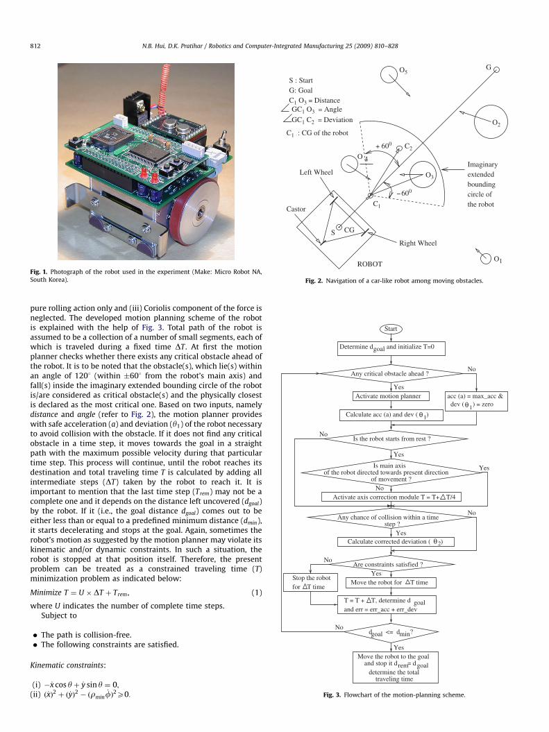
A car-like robot shown in Fig. 1, will be used for testing theperformance of the developed motion planning approaches. It willhave to generate collision-free, time-optimal paths, while navi-gating among some moving obstacles. Kinematic and dynamicconstraints of the car-like robots put restrictions to their motion[2]. Moreover, during navigation, the motion of the robot may beobstructed by the partially unknown movement of the obstacles.
To reduce the complexity of the present problem, the followingassumptions are made: (i) robot’s motion is planned based on asingle critical obstacle, at a time (refer to Fig. 2), (ii) slipping of thewheels of the robot is neglected, they are allowed to move due to
ARTICLE IN PRESS
Fig. 1. Photograph of the robot used in the experiment (Make: Micro Robot NA,
South Korea).
S : StartG: GoalC1 O3 = Distance
GC1 C2 = Deviation
GC1 O3 = Angle
O5G
O2
−600
C2
Left Wheel
Right Wheel
O
O3
O1
4
S CG
ROBOT
Castor
Imaginaryextendedboundingcircle of the robot
+ 600
C1
C1 : CG of the robot
Fig. 2. Navigation of a car-like robot among moving obstacles.
θ1θ1
θ2
Start
Any critical obstacle ahead ?
Activate motion plannerYes
No
Is the robot starts from rest ?
of movement ?of the robot directed towards present direction
Is main axis
step ?Any chance of collision within a time
Are constraints satisfied ?
and err = err_acc + err_dev
Stop the robot
Yes
No
Yes
No
Yes
No
No
acc (a) = max_acc &
T = T + T, determine d goal
goalDetermine d and initialize T=0
for T timeMove the robot for T time
Activate axis correction module T = T+ T/4
dev ( ) = zero
Yes
Calculate acc (a) and dev ( )
Calculate corrected deviation ( )
N.B. Hui, D.K. Pratihar / Robotics and Computer-Integrated Manufacturing 25 (2009) 810–828812
pure rolling action only and (iii) Coriolis component of the force isneglected. The developed motion planning scheme of the robotis explained with the help of Fig. 3. Total path of the robot isassumed to be a collection of a number of small segments, each ofwhich is traveled during a fixed time DT. At first the motionplanner checks whether there exists any critical obstacle ahead ofthe robot. It is to be noted that the obstacle(s), which lie(s) withinan angle of 120� (within �60� from the robot’s main axis) andfall(s) inside the imaginary extended bounding circle of the robotis/are considered as critical obstacle(s) and the physically closestis declared as the most critical one. Based on two inputs, namelydistance and angle (refer to Fig. 2), the motion planner provideswith safe acceleration (a) and deviation (y1) of the robot necessaryto avoid collision with the obstacle. If it does not find any criticalobstacle in a time step, it moves towards the goal in a straightpath with the maximum possible velocity during that particulartime step. This process will continue, until the robot reaches itsdestination and total traveling time T is calculated by adding allintermediate steps (DT) taken by the robot to reach it. It isimportant to mention that the last time step (Trem) may not be acomplete one and it depends on the distance left uncovered (dgoal)by the robot. If it (i.e., the goal distance dgoal) comes out to beeither less than or equal to a predefined minimum distance (dmin),it starts decelerating and stops at the goal. Again, sometimes therobot’s motion as suggested by the motion planner may violate itskinematic and/or dynamic constraints. In such a situation, therobot is stopped at that position itself. Therefore, the presentproblem can be treated as a constrained traveling time (T)minimization problem as indicated below:
Minimize T ¼ U �DT þ Trem, (1)
where U indicates the number of complete time steps.Subject to
d <= d ?goal minNo
�
The path is collision-free.Yes
� The following constraints are satisfied.Move the robot to the goal and stop it d = drem goal
Kinematic constraints:determine the totaltraveling time
(i)
�_x cos yþ _y sin y ¼ 0; Fig. 3. Flowchart of the motion-planning scheme. (ii) ð_xÞ2 þ ð_yÞ2 � ðrmin_fÞ2X0:

ARTICLE IN PRESS
1.0
0.0Mem
bers
hip
Val
ue
V1
VN NR FR VF
Distance (mm)
10 53 106 154
LT AL AH AR RT
Mem
bers
hip
Val
ue 1.0
0.0
Deviation (deg)W1
−60.0 −30.0 0.0 30.0 60.0
LT AL AH AR RT
Mem
bers
hip
Val
ue
V2
1.0
0.0
Angle (deg)
−67.0 −33.5 0.0 33.5 67.0
1.0
0.0Mem
bers
hip
Val
ue
W2
VL L H VH
Acceleration (mm /s )2
5 20.0 35.0 50.0
Fig. 4. Membership function distributions for input and output variables of the FLC.
N.B. Hui, D.K. Pratihar / Robotics and Computer-Integrated Manufacturing 25 (2009) 810–828 813
Dynamic constraints:
(i)
ffiffiffiffiffiffiffiffiffiffiffiffiffiffiffiffiffiffiffiffiffiffiffiffiffiffiffiffiffiffiffiffiðmf gÞ2 � ðV _fÞ2qpap
ffiffiffiffiffiffiffiffiffiffiffiffiffiffiffiffiffiffiffiffiffiffiffiffiffiffiffiffiffiffiffiffiðmf gÞ2 þ ðV _fÞ2
q;
(ii)
aX60P=2pr � GR�M � Nm;where all the notations have their usual meaning.It is important to mention that the minimum traveling time is
possible to achieve, only when the robot traverses through astraight path with the maximum possible velocity of it. To ensurethis, the present problem is solved indirectly by minimizing theerrors due to both deviation output as well as acceleration outputof the motion planner, simultaneously.
3. Developed navigation schemes
Several motion planning schemes have been developed asdiscussed below.
3.1. Approach 1: genetic-fuzzy system
In this approach, an FL-based motion planner is developed forsolving the navigation problems of a real car-like robot. Twoinputs, such as distance of the robot from the most critical obstacleand angle between the line joining the robot and the most criticalobstacle and the reference line (joining the robot and its goal)have been considered for the motion planner and it generates twooutputs, namely deviation and acceleration required by the robotto avoid collision with the obstacle. In the present study, the rangeof distance is divided and represented using four linguistic terms:very near (VN), near (NR), far (FR), very far (VF). Five linguisticterms have been considered for both the angle as well as deviation:left (LT), ahead left (AL), ahead (AH), ahead right (AR) and right(RT) and acceleration is considered to have four terms: very low(VL), low (L), high (H), very high (VH). As there exists a maximumof 20 (i.e., 4� 5) input combinations and for each inputcombination, a maximum of 20 output (i.e., 5� 4) combinationsare possible, a maximum of 400 (i.e., 20� 20) rules are possible.One such rule may look like the following:
IF distance is VF AND angle is LT, THEN deviation is AH andacceleration is VH.
For ease of implementations, membership function distribu-tions of both the input as well as output variables are assumed tobe symmetric triangles (refer to Fig. 4). Thus, the database of theFLC may be modified by using four continuous variablesrepresenting the half base-widths (i.e., V1;V2;W1;W2) of thetriangular membership function distributions. To improve theperformance of FL-based motion planner, an automatic designprocedure of FL using a binary-coded GA is adopted in the presentstudy. A GA-string consisting of 440-bits is considered torepresent the KB of the FLC as shown below:
1::1 0::1 1::0 0::1|fflfflfflfflfflfflfflfflfflfflfflfflfflfflffl{zfflfflfflfflfflfflfflfflfflfflfflfflfflfflffl}Database
10 � � �01|fflfflfflfflffl{zfflfflfflfflffl}Input combinations
101 . . .101 . . .100|fflfflfflfflfflfflfflfflfflfflfflfflfflfflfflffl{zfflfflfflfflfflfflfflfflfflfflfflfflfflfflfflffl}Consequent of the rules
.
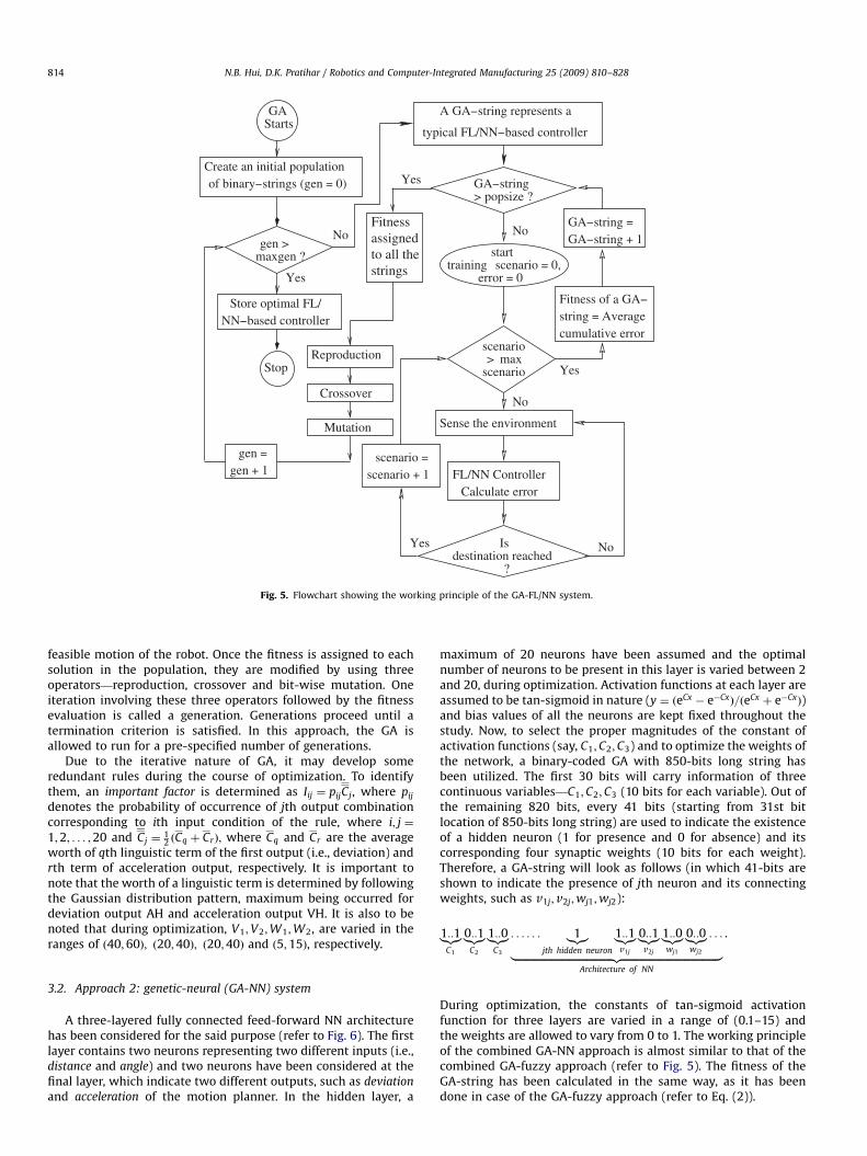
First 40-bits are utilized to represent the database, i.e.,V1;V2;W1;W2 (10 bits for each variable) of the FLC and the next20-bits are used to indicate the presence or absence of the inputcombinations of the RB (1 for presence and 0 for absence). Out ofthe remaining 380-bits, every 19-bits gives the output combina-tion for a particular input combination. The total number of 1’spresent in each 19-bits long sub-string is counted and if it comesout to be equal to zero, it represents the first output combination,i.e., deviation is LT and acceleration is VL, and so on. Fig. 5 showsthe working principle of the combined GA-FLC/NN approach. TheGA begins its search by randomly creating a number of solutions(equals to the population size) represented by the binary strings,each of which indicates a typical FL/NN-based motion planner.Each solution in the population is then evaluated, to assign afitness value. The fitness of a GA-string is calculated using theequation given below:
Fitness ¼1
N
XN
n¼1
1
U
XU
s¼1
X2
v¼1
ðTnsv � OnsvÞ þ Penalty, (2)
where U denotes the total number of time steps in a planned pathand the total number of training scenarios is indicated by N. Onsv
and Tnsv are representing the values of actual and target outputs,respectively, of an output variable (say, v). The target outputs fordeviation and acceleration are taken to be equal to zero andmaximum permissible acceleration of the robot, respectively. Afixed penalty equals to 2000 is added to the fitness of a string, ifthe motion planner represented by it is unable to generate a
ARTICLE IN PRESS
assignedto all thestrings
Fitness
of binary−strings (gen = 0) Create an initial population
GAStarts
Stop
Yes
Store optimal FL/NN−based controller
maxgen ?gen >
gen = gen + 1
scenario =scenario + 1
No
> popsize ?GA−string
error = 0 training scenario = 0,
start
Calculate error
Sense the environment
No
FL/NN Controller
?destination reached
Is NoYes
typical FL/NN−based controller
A GA−string represents a
scenario> max
scenario
Fitness of a GA−string = Averagecumulative error
GA−string = GA−string + 1
Yes
YesReproduction
Crossover
Mutation
No
Fig. 5. Flowchart showing the working principle of the GA-FL/NN system.
N.B. Hui, D.K. Pratihar / Robotics and Computer-Integrated Manufacturing 25 (2009) 810–828814
feasible motion of the robot. Once the fitness is assigned to eachsolution in the population, they are modified by using threeoperators—reproduction, crossover and bit-wise mutation. Oneiteration involving these three operators followed by the fitnessevaluation is called a generation. Generations proceed until atermination criterion is satisfied. In this approach, the GA isallowed to run for a pre-specified number of generations.
Due to the iterative nature of GA, it may develop someredundant rules during the course of optimization. To identifythem, an important factor is determined as Iij ¼ pijCj, where pij
denotes the probability of occurrence of jth output combinationcorresponding to ith input condition of the rule, where i; j ¼
1;2; . . . ;20 and Cj ¼12 ðCq þ CrÞ; where Cq and Cr are the average
worth of qth linguistic term of the first output (i.e., deviation) andrth term of acceleration output, respectively. It is important tonote that the worth of a linguistic term is determined by followingthe Gaussian distribution pattern, maximum being occurred fordeviation output AH and acceleration output VH. It is also to benoted that during optimization, V1;V2;W1;W2, are varied in theranges of ð40;60Þ; ð20;40Þ; ð20;40Þ and ð5;15Þ, respectively.
3.2. Approach 2: genetic-neural (GA-NN) system
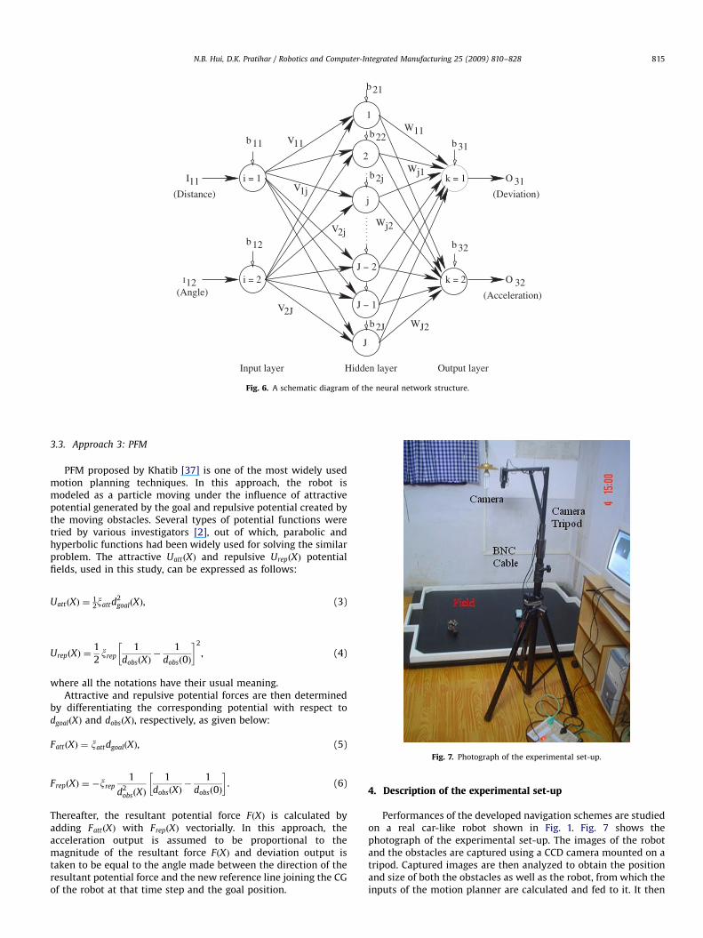
A three-layered fully connected feed-forward NN architecturehas been considered for the said purpose (refer to Fig. 6). The firstlayer contains two neurons representing two different inputs (i.e.,distance and angle) and two neurons have been considered at thefinal layer, which indicate two different outputs, such as deviation
and acceleration of the motion planner. In the hidden layer, a
maximum of 20 neurons have been assumed and the optimalnumber of neurons to be present in this layer is varied between 2and 20, during optimization. Activation functions at each layer areassumed to be tan-sigmoid in nature (y ¼ ðeCx � e�CxÞ=ðeCx þ e�CxÞ)and bias values of all the neurons are kept fixed throughout thestudy. Now, to select the proper magnitudes of the constant ofactivation functions (say, C1;C2;C3) and to optimize the weights ofthe network, a binary-coded GA with 850-bits long string hasbeen utilized. The first 30 bits will carry information of threecontinuous variables—C1;C2;C3 (10 bits for each variable). Out ofthe remaining 820 bits, every 41 bits (starting from 31st bitlocation of 850-bits long string) are used to indicate the existenceof a hidden neuron (1 for presence and 0 for absence) and itscorresponding four synaptic weights (10 bits for each weight).Therefore, a GA-string will look as follows (in which 41-bits areshown to indicate the presence of jth neuron and its connectingweights, such as v1j;v2j;wj1;wj2):
1::1|{z}C1
0::1|{z}C2
1::0|{z}C3
. . . . . . 1|{z}jth hidden neuron
1::1|{z}v1j
0::1|{z}v2j
1::0|{z}wj1
0::0|{z}wj2
. . .
|fflfflfflfflfflfflfflfflfflfflfflfflfflfflfflfflfflfflfflfflfflfflfflfflfflfflfflfflfflfflfflfflfflfflfflfflfflffl{zfflfflfflfflfflfflfflfflfflfflfflfflfflfflfflfflfflfflfflfflfflfflfflfflfflfflfflfflfflfflfflfflfflfflfflfflfflffl}Architecture of NN
.
During optimization, the constants of tan-sigmoid activationfunction for three layers are varied in a range of (0.1–15) andthe weights are allowed to vary from 0 to 1. The working principleof the combined GA-NN approach is almost similar to that of thecombined GA-fuzzy approach (refer to Fig. 5). The fitness of theGA-string has been calculated in the same way, as it has beendone in case of the GA-fuzzy approach (refer to Eq. (2)).
ARTICLE IN PRESS
I12
O 31
32O
W
W11
V
V
V
W11I
(Distance)
(Angle) (Acceleration)
(Deviation)
Input layer Hidden layer Output layer
1
2
i = 2
i = 1
j
V2jj2W
2J
J
J − 2
J − 1
k = 1
k = 2
J2
11
1j
j1
31b
32b
b2J
b2j
b2211b
12b
21b
Fig. 6. A schematic diagram of the neural network structure.
Fig. 7. Photograph of the experimental set-up.
N.B. Hui, D.K. Pratihar / Robotics and Computer-Integrated Manufacturing 25 (2009) 810–828 815
3.3. Approach 3: PFM
PFM proposed by Khatib [37] is one of the most widely usedmotion planning techniques. In this approach, the robot ismodeled as a particle moving under the influence of attractivepotential generated by the goal and repulsive potential created bythe moving obstacles. Several types of potential functions weretried by various investigators [2], out of which, parabolic andhyperbolic functions had been widely used for solving the similarproblem. The attractive UattðXÞ and repulsive UrepðXÞ potentialfields, used in this study, can be expressed as follows:
UattðXÞ ¼ 12xattd
2goalðXÞ, (3)
UrepðXÞ ¼1
2xrep
1
dobsðXÞ�
1
dobsð0Þ
� �2
, (4)
where all the notations have their usual meaning.Attractive and repulsive potential forces are then determined
by differentiating the corresponding potential with respect todgoalðXÞ and dobsðXÞ, respectively, as given below:
FattðXÞ ¼ xattdgoalðXÞ, (5)
FrepðXÞ ¼ �xrep1
d2obsðXÞ
1
dobsðXÞ�
1
dobsð0Þ
� �. (6)
Thereafter, the resultant potential force FðXÞ is calculated byadding FattðXÞ with FrepðXÞ vectorially. In this approach, theacceleration output is assumed to be proportional to themagnitude of the resultant force FðXÞ and deviation output istaken to be equal to the angle made between the direction of theresultant potential force and the new reference line joining the CGof the robot at that time step and the goal position.
4. Description of the experimental set-up
Performances of the developed navigation schemes are studiedon a real car-like robot shown in Fig. 1. Fig. 7 shows thephotograph of the experimental set-up. The images of the robotand the obstacles are captured using a CCD camera mounted on atripod. Captured images are then analyzed to obtain the positionand size of both the obstacles as well as the robot, from which theinputs of the motion planner are calculated and fed to it. It then
ARTICLE IN PRESS
N.B. Hui, D.K. Pratihar / Robotics and Computer-Integrated Manufacturing 25 (2009) 810–828816
determines the safe path of the robot. Thereafter, the informationprovided by the motion planner is communicated to the robot bymeans of a radio-frequency (RF) module.
4.1. Methods of conducting the experiments
The following steps are adopted to conduct the experiment:
�
TabGA-
Dis
VN
VN
VN
NR
NR
FR
FR
VF
VF
VF
Camera calibration: The performance of a CCD camera dependson some of its internal and external parameters. A binary-coded GA is used in the present study, to calibrate it before itcan be used on-line. It is to be mentioned that the calibration isdone off-line [38].
� On-line image processing: The images captured using thecamera are analyzed by developing a suitable image processingmethod, in which the following steps are considered: (i)removal of noise by using a 3� 3 median filter; (ii) binarize theimages by means of a threshold value; (iii) estimation ofperimeters, area with the help of a perimeter descriptor; (iv)labeling of the objects, so as to identify their entity properly;(v) removal of some of the extraneous components based ontheir sizes.
� Control of the robot: Based on the outputs of the motionplanner, the angular speeds of the wheels are derived using aPD control law, which are then communicated to the robot bymeans of a RF module. Finally, actuation of the robot takes
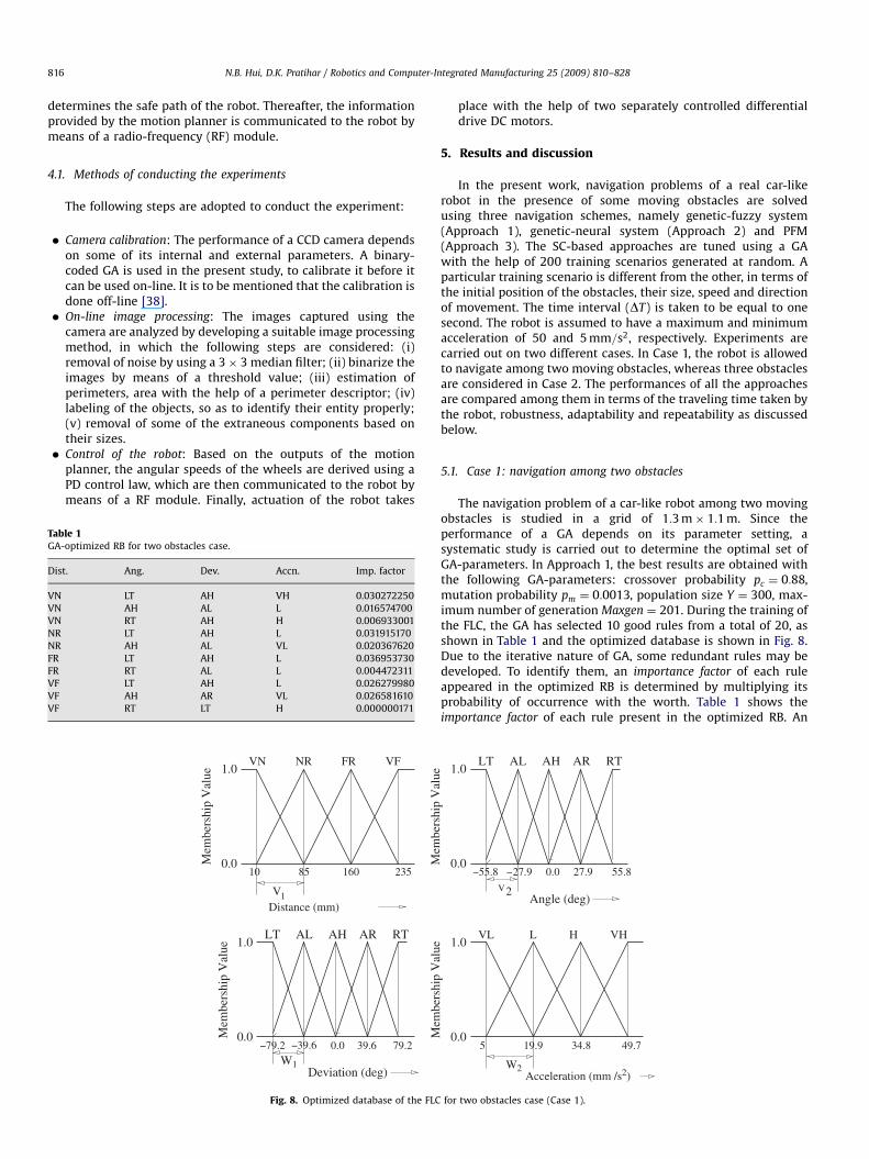
le 1optimized RB for two obstacles case.
t. Ang. Dev. Accn. Imp. factor
LT AH VH 0.030272250
AH AL L 0.016574700
RT AH H 0.006933001
LT AH L 0.031915170
AH AL VL 0.020367620
LT AH L 0.036953730
RT AL L 0.004472311
LT AH L 0.026279980
AH AR VL 0.026581610
RT LT H 0.000000171
1.0
0.0Mem
bers
hip
Val
ue
V1
VN NR FR VF
Distance (mm)
10 85 160 235
LT AL AH AR RT
Mem
bers
hip
Val
ue 1.0
0.0
Deviation (deg)W1
−79.2 −39.6 0.0 39.6 79.2
Fig. 8. Optimized database of the FLC
place with the help of two separately controlled differentialdrive DC motors.
5. Results and discussion
In the present work, navigation problems of a real car-likerobot in the presence of some moving obstacles are solvedusing three navigation schemes, namely genetic-fuzzy system(Approach 1), genetic-neural system (Approach 2) and PFM(Approach 3). The SC-based approaches are tuned using a GAwith the help of 200 training scenarios generated at random. Aparticular training scenario is different from the other, in terms ofthe initial position of the obstacles, their size, speed and directionof movement. The time interval (DT) is taken to be equal to onesecond. The robot is assumed to have a maximum and minimumacceleration of 50 and 5 mm=s2, respectively. Experiments arecarried out on two different cases. In Case 1, the robot is allowedto navigate among two moving obstacles, whereas three obstaclesare considered in Case 2. The performances of all the approachesare compared among them in terms of the traveling time taken bythe robot, robustness, adaptability and repeatability as discussedbelow.
5.1. Case 1: navigation among two obstacles
The navigation problem of a car-like robot among two movingobstacles is studied in a grid of 1:3 m� 1:1 m. Since theperformance of a GA depends on its parameter setting, asystematic study is carried out to determine the optimal set ofGA-parameters. In Approach 1, the best results are obtained withthe following GA-parameters: crossover probability pc ¼ 0:88,mutation probability pm ¼ 0:0013, population size Y ¼ 300, max-imum number of generation Maxgen ¼ 201. During the training ofthe FLC, the GA has selected 10 good rules from a total of 20, asshown in Table 1 and the optimized database is shown in Fig. 8.Due to the iterative nature of GA, some redundant rules may bedeveloped. To identify them, an importance factor of each ruleappeared in the optimized RB is determined by multiplying itsprobability of occurrence with the worth. Table 1 shows theimportance factor of each rule present in the optimized RB. An
LT AL AH AR RT
Mem
bers
hip
Val
ue
V2
1.0
0.0
Angle (deg)
−55.8 −27.9 0.0 27.9 55.8
1.0
0.0Mem
bers
hip
Val
ue
W2
VL L H VH
Acceleration (mm /s2)
49.734.819.95
for two obstacles case (Case 1).
ARTICLE IN PRESS
N.B. Hui, D.K. Pratihar / Robotics and Computer-Integrated Manufacturing 25 (2009) 810–828 817
experiment is also carried out to check whether the GA-designedRB contains any redundant rule. When the FLC is run with eightoptimal rules after removing the 10-th and 7-th rules of Table 1
Table 2Rules present in the RB vs. non-firing incidences.
Rules present in
RB
Rule no. made
absent
No. of non-firing
incidences
Traveling time
(seconds)
10 – 0 22.664
09 10 0 22.664
08 10;7 0 22.664
07 10;0;3 161 45.035
06 10;7;3;2 212 51.577
05 10;7;3;2;5 417 58.380
Table 3Comparison of three approaches in terms of traveling time in seconds—(Case 1).
Scen. no. Approach 1 Approach 2 Approach 3
1 37 36 40
2 39 42 47
3 42 37 57
4 40 36 48
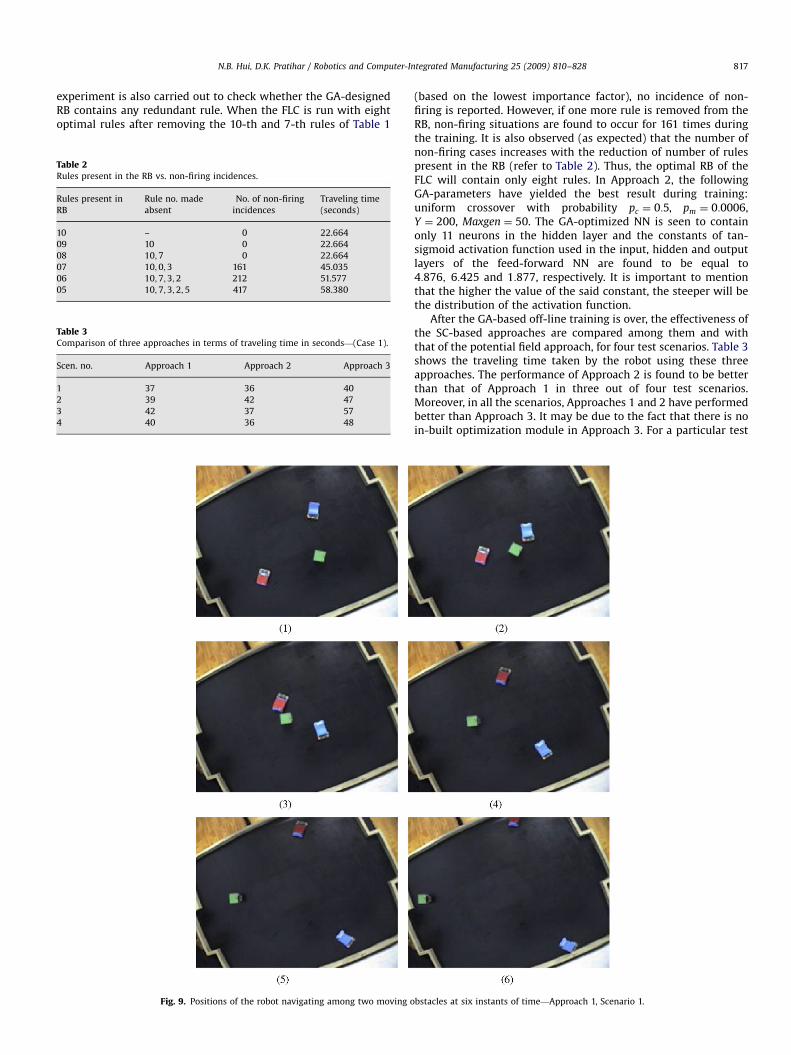
Fig. 9. Positions of the robot navigating among two moving o
(based on the lowest importance factor), no incidence of non-firing is reported. However, if one more rule is removed from theRB, non-firing situations are found to occur for 161 times duringthe training. It is also observed (as expected) that the number ofnon-firing cases increases with the reduction of number of rulespresent in the RB (refer to Table 2). Thus, the optimal RB of theFLC will contain only eight rules. In Approach 2, the followingGA-parameters have yielded the best result during training:uniform crossover with probability pc ¼ 0:5, pm ¼ 0:0006,Y ¼ 200, Maxgen ¼ 50. The GA-optimized NN is seen to containonly 11 neurons in the hidden layer and the constants of tan-sigmoid activation function used in the input, hidden and outputlayers of the feed-forward NN are found to be equal to4:876; 6:425 and 1:877, respectively. It is important to mentionthat the higher the value of the said constant, the steeper will bethe distribution of the activation function.
After the GA-based off-line training is over, the effectiveness ofthe SC-based approaches are compared among them and withthat of the potential field approach, for four test scenarios. Table 3shows the traveling time taken by the robot using these threeapproaches. The performance of Approach 2 is found to be betterthan that of Approach 1 in three out of four test scenarios.Moreover, in all the scenarios, Approaches 1 and 2 have performedbetter than Approach 3. It may be due to the fact that there is noin-built optimization module in Approach 3. For a particular test
bstacles at six instants of time—Approach 1, Scenario 1.
ARTICLE IN PRESS
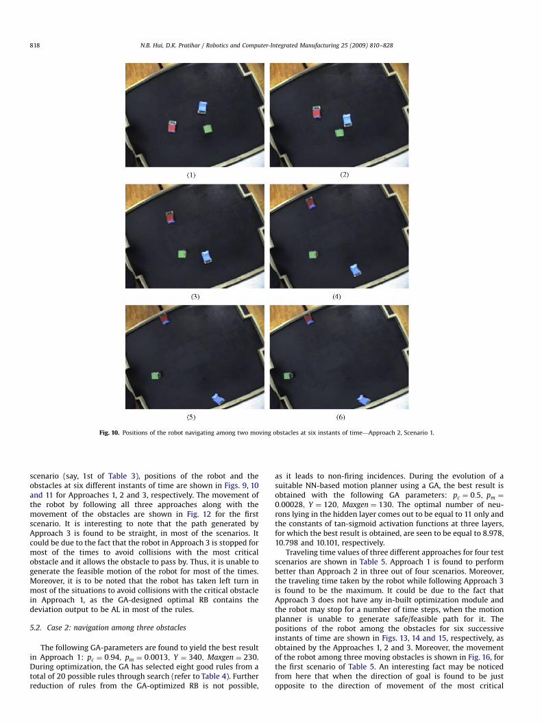
Fig. 10. Positions of the robot navigating among two moving obstacles at six instants of time—Approach 2, Scenario 1.
N.B. Hui, D.K. Pratihar / Robotics and Computer-Integrated Manufacturing 25 (2009) 810–828818
scenario (say, 1st of Table 3), positions of the robot and theobstacles at six different instants of time are shown in Figs. 9, 10and 11 for Approaches 1, 2 and 3, respectively. The movement ofthe robot by following all three approaches along with themovement of the obstacles are shown in Fig. 12 for the firstscenario. It is interesting to note that the path generated byApproach 3 is found to be straight, in most of the scenarios. Itcould be due to the fact that the robot in Approach 3 is stopped formost of the times to avoid collisions with the most criticalobstacle and it allows the obstacle to pass by. Thus, it is unable togenerate the feasible motion of the robot for most of the times.Moreover, it is to be noted that the robot has taken left turn inmost of the situations to avoid collisions with the critical obstaclein Approach 1, as the GA-designed optimal RB contains thedeviation output to be AL in most of the rules.
5.2. Case 2: navigation among three obstacles
The following GA-parameters are found to yield the best resultin Approach 1: pc ¼ 0:94; pm ¼ 0:0013; Y ¼ 340; Maxgen ¼ 230.During optimization, the GA has selected eight good rules from atotal of 20 possible rules through search (refer to Table 4). Furtherreduction of rules from the GA-optimized RB is not possible,
as it leads to non-firing incidences. During the evolution of asuitable NN-based motion planner using a GA, the best result isobtained with the following GA parameters: pc ¼ 0:5; pm ¼
0:00028; Y ¼ 120; Maxgen ¼ 130. The optimal number of neu-rons lying in the hidden layer comes out to be equal to 11 only andthe constants of tan-sigmoid activation functions at three layers,for which the best result is obtained, are seen to be equal to 8.978,10.798 and 10.101, respectively.
Traveling time values of three different approaches for four testscenarios are shown in Table 5. Approach 1 is found to performbetter than Approach 2 in three out of four scenarios. Moreover,the traveling time taken by the robot while following Approach 3is found to be the maximum. It could be due to the fact thatApproach 3 does not have any in-built optimization module andthe robot may stop for a number of time steps, when the motionplanner is unable to generate safe/feasible path for it. Thepositions of the robot among the obstacles for six successiveinstants of time are shown in Figs. 13, 14 and 15, respectively, asobtained by the Approaches 1, 2 and 3. Moreover, the movementof the robot among three moving obstacles is shown in Fig. 16, forthe first scenario of Table 5. An interesting fact may be noticedfrom here that when the direction of goal is found to be justopposite to the direction of movement of the most critical

ARTICLE IN PRESS
Fig. 11. Positions of the robot navigating among two moving obstacles at six instants of time—Approach 3, Scenario 1.
Fig. 12. Movement of the robot among two moving obstacles in Scenario 1.
Table 4GA-optimized RB for two obstacles case.
Dist. Ang. Dev. Accn. Imp. factor
VN AL AR L 0.00976309
VN AR AL VL 0.00689057
NR AL AR L 0.01533519
FR LT AR L 0.00388311
FR AR AH H 0.03434102
FR RT AH VL 0.00449050
VF AL AH L 0.02119378
VF AR AL L 0.01710485
Table 5Comparison of three approaches in terms of traveling time in seconds—(Case 2).
Scen. no. Approach 1 Approach 2 Approach 3
1 31 32 37
2 37 35 45
3 38 43 46
4 36 39 44
N.B. Hui, D.K. Pratihar / Robotics and Computer-Integrated Manufacturing 25 (2009) 810–828 819
obstacle, the robot using the PFM moves straight towards the goalwith a very low speed and as a result of which, the robot takesmore time to reach the goal. Thus, the shortest distance path
obtained by Approach 3 may not always be the time-optimal one.However, the SC-based motion planners are seen to tackle suchsituations effectively. It may be due to the fact that the SC-based

ARTICLE IN PRESS
Fig. 13. Positions of the robot navigating among three moving obstacles at six instants of time—Approach 1, Scenario 1.
N.B. Hui, D.K. Pratihar / Robotics and Computer-Integrated Manufacturing 25 (2009) 810–828820
approaches may have some adaptability. It is important tomention that some actuation error of the motors has been noticed,while performing the experiment. It might have happened due tothe time lag between the consecutive communication signals andfluctuations in the supplied voltage of the battery. The developedmotion planners have also been compared among them in terms ofrobustness, adaptability and reliability, which are discussed below.
5.3. Robustness test
A motion planner will be called robust, if it can accommodatesome variations/errors during its execution, such as modelingvariations, motion variations, sensing errors, motion errors andothers [39]. In the present work, six different variations have beenconsidered, which are discussed below. Five different testscenarios are solved by varying the size of the obstacles andkeeping the other parameters (i.e., velocities of the obstacles,their directions of movement, starting positions, starting andgoal positions of the robot) unchanged. The variations in travelingtime due to it, are shown in Table 6 for all three approaches.The standard deviation (SD) of the traveling time values forApproach 1 comes out to be less compared to that forthe Approaches 2 and 3. It may be due to the fact that
Approach 1 is less sensitive to the size variations of the obstacles,i.e., more robust. Movements of the robot among two movingobstacles for all the above five different scenarios are shown inFig. 17.
In the similar way, one of the remaining parameters has beenchanged at a time keeping the others fixed and for each of them,five test scenarios are considered. Traveling time values of threeapproaches for the above experiments are tabulated in Table 6.Approach 1 is found to be more robust compared to the other twomotion planners with respect to the variations of obstacles’velocities, initial positions of the obstacles, initial and goalpositions of the robot, whereas Approach 2 has shown itsrobustness against the variations of the obstacles’ direction ofmovement. Thus, it can be concluded that the SC-basedapproaches can accommodate small changes in the environmentalmodel. On the other hand, the PFM has yielded large variations intraveling time even for small changes of the above parameters.Thus, it is seen to be less robust compared to the other two motionplanners. Figs. 18–22 show the paths of the robot planned by threeapproaches, after allowing small changes of the above parameters.It is important to mention that Approach 3 has generated theshortest path (in terms of distance) for more times compared tothe Approaches 1 and 2 but it is unable to generate the feasible
ARTICLE IN PRESS
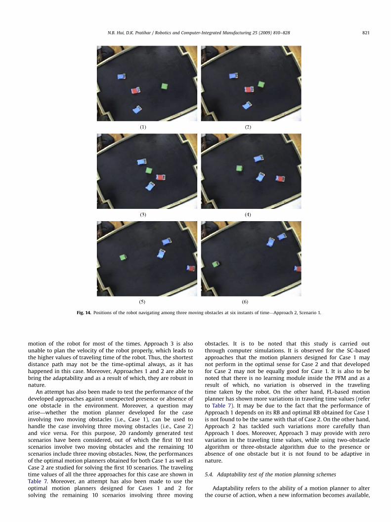
Fig. 14. Positions of the robot navigating among three moving obstacles at six instants of time—Approach 2, Scenario 1.
N.B. Hui, D.K. Pratihar / Robotics and Computer-Integrated Manufacturing 25 (2009) 810–828 821
motion of the robot for most of the times. Approach 3 is alsounable to plan the velocity of the robot properly, which leads tothe higher values of traveling time of the robot. Thus, the shortestdistance path may not be the time-optimal always, as it hashappened in this case. Moreover, Approaches 1 and 2 are able tobring the adaptability and as a result of which, they are robust innature.
An attempt has also been made to test the performance of thedeveloped approaches against unexpected presence or absence ofone obstacle in the environment. Moreover, a question mayarise—whether the motion planner developed for the caseinvolving two moving obstacles (i.e., Case 1), can be used tohandle the case involving three moving obstacles (i.e., Case 2)and vice versa. For this purpose, 20 randomly generated testscenarios have been considered, out of which the first 10 testscenarios involve two moving obstacles and the remaining 10scenarios include three moving obstacles. Now, the performancesof the optimal motion planners obtained for both Case 1 as well asCase 2 are studied for solving the first 10 scenarios. The travelingtime values of all the three approaches for this case are shown inTable 7. Moreover, an attempt has also been made to use theoptimal motion planners designed for Cases 1 and 2 forsolving the remaining 10 scenarios involving three moving
obstacles. It is to be noted that this study is carried outthrough computer simulations. It is observed for the SC-basedapproaches that the motion planners designed for Case 1 maynot perform in the optimal sense for Case 2 and that developedfor Case 2 may not be equally good for Case 1. It is also to benoted that there is no learning module inside the PFM and as aresult of which, no variation is observed in the travelingtime taken by the robot. On the other hand, FL-based motionplanner has shown more variations in traveling time values (referto Table 7). It may be due to the fact that the performance ofApproach 1 depends on its RB and optimal RB obtained for Case 1is not found to be the same with that of Case 2. On the other hand,Approach 2 has tackled such variations more carefully thanApproach 1 does. Moreover, Approach 3 may provide with zerovariation in the traveling time values, while using two-obstaclealgorithm or three-obstacle algorithm due to the presence orabsence of one obstacle but it is not found to be adaptive innature.
5.4. Adaptability test of the motion planning schemes
Adaptability refers to the ability of a motion planner to alterthe course of action, when a new information becomes available,

ARTICLE IN PRESS
Fig. 15. Positions of the robot navigating among three moving obstacles at six instants of time—Approach 3, Scenario 1.
Fig. 16. Movement of the robot among three moving obstacles in Scenario 1.
N.B. Hui, D.K. Pratihar / Robotics and Computer-Integrated Manufacturing 25 (2009) 810–828822
like in urgency. According to Smith [40], one or more of thefollowing requirements is/are to be fulfilled by an adaptivesystem: (i) it must generate an acceptable behavior (i.e., stable
solutions) always and must not behave excessively strange in theadaptation phase; (ii) it must not require any special training orhelp from the trained staff and (iii) it should be general.
In the present study, three different motion planning schemeshave been developed and their effectiveness are studied forsolving two different cases, as described earlier. In both the cases,traveling time taken by the robot using Approach 3 comes out tobe the maximum. It has happened due to the fact that thepotential field-based motion planner is unable to generate feasiblesolutions (i.e., stable solutions) always. The situation becomesmore complex, when the obstacles come towards the robot ormove perpendicular to the goal line. On the other hand, SC-basedmotion planners are found to tackle those situations tactfully. Itcould be due to the fact that both the SC-based approaches couldunderstand such situations well. It is also to be noted that all theapproaches are designed in such a way that the robot can stopsmoothly after reaching the goal. Moreover, magnitude ofattractive force is considered to be proportional to the distancebetween the robot and its goal in Approach 3 and as a result ofwhich, if the robot faces any critical obstacle near to the goal, itmoves very slowly. This particular aspect deteriorates theperformance of this approach to a great extent. However, boththe SC-based approaches behave in a similar manner irrespectiveof the distance between the robot and the goal. Therefore, both

ARTICLE IN PRESS
Table 6Traveling time (seconds) variations due to the small changes in the environment
model.
Scen. no. Approach 1 Approach 2 Approach 3
(a) Size variations of the obstacles
1 32.632 33.250 34.407
2 37.100 42.823 47.038
3 35.286 42.073 54.819
4 30.289 42.073 46.210
5 30.158 41.062 49.250
SD 2.988 4.550 8.420
(b) Velocity variations of the obstacles
1 32.632 33.250 34.407
2 37.100 42.823 47.038
3 35.286 42.073 54.819
4 30.289 42.073 46.210
5 30.158 41.062 49.250
SD 2.988 4.550 8.420
(c) Direction variations of the obstacles
1 35.124 42.073 43.160
2 34.158 42.073 55.282
3 35.286 42.073 54.819
4 29.632 42.073 54.208
5 46.951 42.073 54.107
SD 2.659 0.000 5.821
(d) Initial position variations of the obstacles
1 30.483 43.332 54.238
2 30.808 35.043 47.071
3 35.286 42.073 54.819
4 30.424 39.657 46.157
5 30.962 33.250 34.407
SD 2.077 4.382 8.250
(e) Starting position variations of the robot
1 29.657 38.622 50.222
2 33.100 35.250 41.250
3 35.286 42.073 54.819
4 32.100 35.875 37.250
5 32.100 36.209 54.831
SD 2.032 2.806 8.042
(f) Goal position variations of the robot
1 29.100 27.871 45.822
2 23.595 26.185 38.234
3 35.286 42.073 54.819
4 30.324 31.470 51.090
5 35.100 29.761 49.250
SD 4.836 6.249 6.277
N.B. Hui, D.K. Pratihar / Robotics and Computer-Integrated Manufacturing 25 (2009) 810–828 823
the FL- as well as NN-based approaches are able to generate therobot’s motion in a more adaptive way.
5.5. Reliability of the motion planning schemes
Reliability of a motion planning scheme has been defined in anumber of ways. According to Hwang et al. [41], it is a mixtureof consistency and repeatability. Kim et al. [31] in their bookentitled soccer robotics mentioned that reliability refers to thedependability of a system (i.e., whether it functions properly eachtime it is utilized) and for achieving it, a system will have to beadaptive in nature. According to Roy and Thrun [42], reliabilitymeans goal reaching capability, i.e., it is the capability with whichthe robot can reach the goal in most of the times. On the otherhand, Alami et al. [43] considered it to be equivalent with theconsistent behavior. An attempt has been made to test thereliability of the developed navigation schemes, in this study. For
this purpose, both the repeatability as well as goal reachingcapability of the three approaches have been analyzed, as givenbelow.
5.5.1. Repeatability test of the motion planning schemes
Repeatability is an issue to be considered related to anyexperimental result for ensuring the reliable performance of thedeveloped approaches. For this purpose, all the three approacheshave been used separately to solve a particular scenario involvingtwo moving obstacles for three times each. Traveling time valuestaken by the robot for the three approaches are shown in Table 8for the three trials. Fig. 23 shows the movement of the obstaclesand variations of the path planned by the robot during three trialsusing Approaches 1–3. It is to be noticed that there exists a slightvariation in both the traveling time as well as the paths plannedby the robot for all the approaches, which might have come due tothe following reasons:
�
Developed image acquisition system is very sensitive to theintensity of light. Thus, a slight fluctuation of light intensitymay give rise to wrong position information of the movingobjects, leading to performance deterioration of the motionplanners. � Actuation error of the robot may exist due to fluctuations in thevoltage supplied by the dry cells used in this study.
� Movements of the obstacles are not made automatic, they arebattery driven but manually operated. Thus, a slight fluctua-tion in the movement of the obstacles may yield a considerablevariation in movement of the robot.
5.5.2. Goal reaching capability
It is the ability of the robot to reach the goal accurately.However, a close watch on the results reveals that goal reachingcapability of the NN-based motion planner is better than that ofthe FL-based approach. It may be due to the reason that the robotusing Approach 1 is taking the maximum turn to avoid collisionswith the obstacles and moving with the high speed. However, it isdependent on its KB. On the other hand, the PFM is unable toprovide with feasible solutions and consequently, stops for mostof the times, while avoiding collision with the obstacles. Thus, itgenerates the straight path for most of the steps and reaches thegoal accurately for most of the times.
6. Concluding remarks
The prime aim of this study is to develop an adaptivenavigation scheme for a real car-like robot navigating amongsome moving obstacles. Both FL- as well as NN-based motionplanners (i.e., Approaches 1 and 2) had been developed by thesame authors in the past and their performances were comparedamong them and with that of a PFM (i.e., Approach 3) throughcomputer simulations. In the present study, an attempt is madeto test the effectiveness of Approaches 1–3 on a real car-like robot,so as to identify the best one in terms of traveling time,robustness, adaptability, reliability and others. Training to boththe FL- as well as NN-based motion planner is given off-line usinga GA. Once the optimization is over for the SC-based approaches,their performances are compared among them and with that ofthe PFM for solving the navigation problems of a real wheeledrobot. The following conclusions have been drawn from thepresent study:
�
Computational complexities of Approaches 1, 2 and 3 areseen to be equal to 0:023, 0:018 and 0:013 seconds,
ARTICLE IN PRESS
Fig. 17. Movement of the robot among two moving obstacles having different radii, in m: (a) r1 ¼ 0:040; r2 ¼ 0:020, (b) r1 ¼ 0:044; r2 ¼ 0:022, (c) r1 ¼ 0:048; r2 ¼ 0:024,
(d) r1 ¼ 0:052; r2 ¼ 0:026, (e) r1 ¼ 0:056; r2 ¼ 0:028.
Fig. 18. Movement of the robot among two moving obstacles having different velocities (m/s): (a) v1 ¼ 0:028; v2 ¼ 0:009, (b) v1 ¼ 0:030; v2 ¼ 0:011,
(c) v1 ¼ 0:034; v2 ¼ 0:013, (d) v1 ¼ 0:036; v2 ¼ 0:015, (e) v1 ¼ 0:038; v2 ¼ 0:017.
N.B. Hui, D.K. Pratihar / Robotics and Computer-Integrated Manufacturing 25 (2009) 810–828824
respectively. Thus, they are suitable for on-line implementa-tions.
� During the training, time taken to converge to a fixedaccuracy level by the FL-based approach is seen to be lowercompared to that of the NN-based motion planner. It may be
due to the fact that a larger binary string is required torepresent an NN compared to that necessary for indicatingan FLC.
� The performances of both the SC-based approaches are foundto be comparable. However, traveling time taken by the robot

ARTICLE IN PRESS
Fig. 19. Movement of the robot among two obstacles moving in different directions (radian): (a) y1 ¼ 2:204; y2 ¼ 3:065, (b) y1 ¼ 2:304; y2 ¼ 3:115, (c) y1 ¼ 2:404;
y2 ¼ 3:165, (d) y1 ¼ 2:504, y2 ¼ 3:215, (e) y1 ¼ 2:604; y2 ¼ 3:265.
Fig. 20. Movement of the robot among two moving obstacles starting from different initial positions (m): (a) ð0:903;0:743Þ; ð0:728;0:389Þ, (b) ð0:803;0:843Þ; ð0:628;0:489Þ,
(c) ð0:903;0:843Þ; ð0:728;0:489Þ, (d) ð1:003;0:843Þ, ð0:828;0:489Þ, (e) ð0:903;0:943Þ; ð0:728;0:589Þ.
N.B. Hui, D.K. Pratihar / Robotics and Computer-Integrated Manufacturing 25 (2009) 810–828 825
in Approach 3 has come out to be the maximum in most of thecases. It may be due to the reason that there is no in-builtoptimization module in the PFM.
�
In some scenarios, the robot using Approach 3, has failedto find any feasible solution. This may happen, whenthe repulsive potential balances the attractive potential or
ARTICLE IN PRESS
Fig. 21. Movement of the robot among two moving obstacles, initiating its motion from different starting positions (m): (a) ð0:30;0:35Þ, (b) ð0:45;0:20Þ, (c) ð0:300;0:200Þ,
(d) ð0:30;0:05Þ, (e) ð0:15;0:20Þ.
Fig. 22. Movement of the robot among two moving obstacles, while reaching different goal positions: (a) ð0:9 m;0:9 mÞ, (b) ð0:9 m;0:7 mÞ, (c) ð1:3 m;1:1 mÞ,
(d) ð1:1 m;1:1 mÞ, (e) ð1:1 m;0:9 mÞ.
N.B. Hui, D.K. Pratihar / Robotics and Computer-Integrated Manufacturing 25 (2009) 810–828826
the motion generated by Approach 3 has failed due to thekinematic and/or dynamic constraints of the robot.
� SC-based approaches are found to be more robust andadaptive than the conventional PFM. It may be due to thefact that the PFM does not have any in-built learning module.
All the parameters used in this approach are static innature and do not adapt automatically, as the situationchanges.
� It is to be noted that all the approaches are found to be reliablein terms of repeatability and goal reaching capability.
ARTICLE IN PRESS
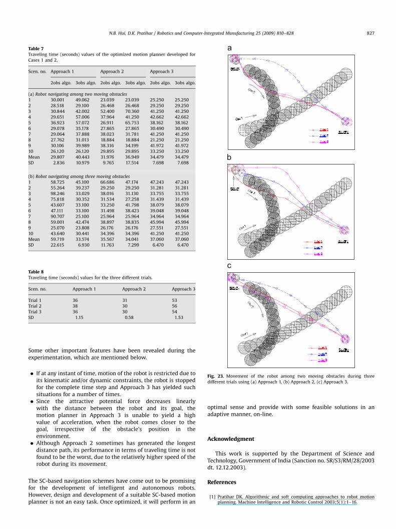
Table 7Traveling time (seconds) values of the optimized motion planner developed for
Cases 1 and 2.
Scen. no. Approach 1 Approach 2 Approach 3
2obs algo. 3obs algo. 2obs algo. 3obs algo. 2obs algo. 3obs algo.
(a) Robot navigating among two moving obstacles
1 30.001 49.062 23.039 23.039 25.250 25.250
2 28.518 29.100 26.468 26.468 29.250 29.250
3 30.844 42.002 52.400 70.360 41.250 41.250
4 29.651 57.006 37.964 41.250 42.662 42.662
5 36.923 57.072 26.911 65.753 38.162 38.162
6 29.078 35.178 27.865 27.865 30.490 30.490
7 29.064 37.888 38.023 31.781 41.250 41.250
8 27.762 31.013 18.884 18.884 21.250 21.250
9 30.106 39.989 38.316 34.199 41.972 41.972
10 26.120 26.120 29.895 29.895 33.250 33.250
Mean 29.807 40.443 31.976 36.949 34.479 34.479
SD 2.836 10.979 9.765 17.514 7.698 7.698
(b) Robot navigating among three moving obstacles
1 58.725 45.100 66.686 47.174 47.243 47.243
2 55.264 39.237 29.250 29.250 31.281 31.281
3 98.246 33.029 38.016 31.130 33.755 33.755
4 75.818 30.352 31.534 27.258 31.439 31.439
5 43.607 33.100 33.250 41.798 38.079 38.079
6 47.111 33.100 31.498 38.423 39.048 39.048
7 90.707 25.100 25.964 25.964 34.964 34.964
8 59.001 42.474 38.897 38.835 45.994 45.994
9 25.070 23.808 26.176 26.176 27.551 27.551
10 43.640 30.441 34.396 34.396 41.250 41.250
Mean 59.719 33.574 35.567 34.041 37.060 37.060
SD 22.615 6.930 11.763 7.299 6.470 6.470
Table 8Traveling time (seconds) values for the three different trials.
Scen. no. Approach 1 Approach 2 Approach 3
Trial 1 36 31 53
Trial 2 38 30 56
Trial 3 36 30 54
SD 1.15 0.58 1.53
N.B. Hui, D.K. Pratihar / Robotics and Computer-Integrated Manufacturing 25 (2009) 810–828 827
Some other important features have been revealed during theexperimentation, which are mentioned below.
�
Fig. 23. Movement of the robot among two moving obstacles during threedifferent trials using (a) Approach 1, (b) Approach 2, (c) Approach 3.
If at any instant of time, motion of the robot is restricted due toits kinematic and/or dynamic constraints, the robot is stoppedfor the complete time step and Approach 3 has yielded suchsituations for a number of times.
� Since the attractive potential force decreases linearlywith the distance between the robot and its goal, themotion planner in Approach 3 is unable to yield a highvalue of acceleration, when the robot comes closer to thegoal, irrespective of the obstacle’s position in theenvironment.
� Although Approach 2 sometimes has generated the longestdistance path, its performance in terms of traveling time is notfound to be the worst, due to the relatively higher speed of therobot during its movement.
The SC-based navigation schemes have come out to be promisingfor the development of intelligent and autonomous robots.However, design and development of a suitable SC-based motionplanner is not an easy task. Once optimized, it will perform in an
optimal sense and provide with some feasible solutions in anadaptive manner, on-line.
Acknowledgment
This work is supported by the Department of Science andTechnology, Government of India (Sanction no. SR/S3/RM/28/2003dt. 12.12.2003).
References
[1] Pratihar DK. Algorithmic and soft computing approaches to robot motionplanning. Machine Intelligence and Robotic Control 2003;5(1):1–16.
ARTICLE IN PRESS
N.B. Hui, D.K. Pratihar / Robotics and Computer-Integrated Manufacturing 25 (2009) 810–828828
[2] Latombe J-C. Robot motion planning. Dordrecht: Kluwer Academic Publisher;1991.
[3] Liu YH, Arimoto S. Path planning using a tangent graph for mobile robotsamong polynomial and curved obstacles. The International Journal ofRobotics Research 1992;11(4):376–82.
[4] Kant K, Zucker SW. Towards efficient planning: the path velocity decomposi-tion. The International Journal of Robotics Research 1986;5(1):72–89.
[5] Fujimura K, Samet H. Accessibility: a new approach to path planning amongmoving obstacles. In: Proceedings of IEEE conference on computer vision andpattern recognition, Ann Arbor, MI, 1988. p. 803–7.
[6] Lamadrid JG, Gini ML. Path tracking through uncharted moving obstacles.IEEE Transactions on Systems, Man and Cybernetics 1990;20(6):1408–22.
[7] Slack MG, Miller DP. Path planning through time and space in dynamicdomains. In: Proceedings of the international joint conference on artificialintelligence; 1987. p. 1067–70.
[8] Fiorini P, Shiller Z. Motion planning in dynamic environments using therelative velocity paradigm. In: Proceedings of IEEE conference on robotics andautomation; 1993. p. 560–5.
[9] Brooks RA. A robust layered control system for a mobile robot. IEEETransactions on Robotics and Automation 1986;RA-2:14–23.
[10] Simmons R. The curvature-velocity method for local obstacle avoidance. In:Proceedings of the international conference on robotics and automation, vol.4; 1996. p. 2275–82.
[11] Fox D, Burgard W, Thrun S. The dynamic window approach to collisionavoidance. IEEE Robotics & Automation Magazine 1997;23:23–33.
[12] LaValle SM, Kuffner JJ. Randomized kinodynamic planning. InternationalJournal of Robotics Research 2001;20(5):378–400.
[13] Koren Y, Borenstein J. Potential field methods and their inherent limitationsfor mobile robot navigation. In: Proceedings of the IEEE conference onrobotics and automation, Sacramento, CA, 1991. p. 1398–404.
[14] Borenstein J, Koren Y. Real time obstacle avoidance for fast mobile robots.IEEE Transactions on Systems Man and Cybernetics 1989;19(5):1179–87.
[15] Ulrich I, Borenstein J. Vfh+: reliable obstacle avoidance for fast mobile robots.In: Proceedings of the IEEE international conference on robotics andautomation (ICRA); 1998.
[16] Ge S, Cui Y. Dynamic motion planning for mobile robots using potential fieldmethod. Autonomous Robots 2002;13:207–22.
[17] Fraichard T, Scheuer A. Car-like robots and moving obstacles. In: Proceedingsof IEEE conference on robotics and automation; 1996. p. 64–9.
[18] Abdessemed F, Benmahammed K, Monacelli E. A fuzzy-based reactivecontroller for a non-holonomic mobile robot. Robotics and AutonomousSystems 2004;47:31–46.
[19] Song KT, Sheen LH. Heuristic fuzzy-neuro network and its application toreactive navigation of a mobile robot. Fuzzy Sets and Systems 2000;110:331–40.
[20] Li W, Ma C, Wahl FM. A neuro-fuzzy system architecture for behavior basedcontrol of a mobile robot in unknown environments. Fuzzy Sets and Systems1997;87:133–40.
[21] Marichal GN, Acosta L, Moreno L, Mendez J, Rodrigo J, Sigut M. Obstacleavoidance for a mobile robot: a neuro fuzzy approach. Fuzzy Sets and Systems2001;124:171–9.
[22] Pratihar DK, Bibel W. Near-optimal, collision-free path generation formultiple robots working in the same workspace using a genetic-fuzzysystems. Machine Intelligence and Robotic Control 2003;5(2):45–58.
[23] Hui NB, Pratihar DK. Mobile robot navigation: potential field approach vs.genetic-fuzzy system. In: Proceedings of 10th on-line world conference onsoft computing (WSC10); 2005.
[24] Yang SX, Meng M. An efficient neural network approach to dynamic robotmotion planning. Neural Networks 2000;13(2):143–8.
[25] Mondada F, Floreano D. Evolution of neural control structures: someexperiments on mobile robots. Robotics and Autonomous Systems 1995;16:183–95.
[26] Pal PK, Kar A. Sonar-based mobile robot navigation through supervisedlearning on a neural net. Autonomous Robots 1996;3:355–74.
[27] Gu D, Hu H. Neural predictive control for a car-like mobile robot. Robotics andAutonomous Systems 2002;39:73–86.
[28] Goldberg DE. Genetic algorithms in search, optimization, machine learning.Reading, MA, USA: Addison-Wesley; 1989.
[29] Pratihar DK. Evolutionary robotics—a review. Sadhana 2003;28(6):999–1003.[30] Thrun S. An approach to learning mobile robot navigation. Robotics and
Autonomous Systems 1996;15:301–9.[31] Kim J-H, Kim D-H, Kim Y-J, Seow K-T. Soccer robotics. Amsterdam: Springer;
2004.[32] Akbarzadeh M, Kumbla K, Tunstel E, Jamshidi M. Soft computing for
autonomous robotic systems. Computers and Electrical Engineering 2000;26:5–32.
[33] Ohya A, Kosaka A, Kak A. Vision-based navigation by a mobile robot withobstacle avoidance using single-camera vision and ultrasonic sensing. IEEETransactions of Robotics and Automation 1998;14(8):969–78.
[34] Zhang S, Xie L, Adams MD. Feature extraction for outdoor mobile robotnavigation based on a modified Gauss–Newton optimization approach.Robotics and Autonomous Systems 2006;54:277–87.
[35] Hui NB, Pratihar DK. Neural network-based approaches vs potential fieldapproach for solving navigation problems of a car-like robot. MachineIntelligence and Robotic Control 2004;6(2):39–60.
[36] Hui NB, Pratihar DK. Automatic design of fuzzy logic controller usinga genetic algorithm for collision-free, time-optimal navigation of a car-like robot. International Journal of Hybrid Intelligent Systems 2005;5(3):161–87.
[37] Khatib O. Real-time obstacle avoidance for manipulators and mobile robots.The International Journal of Robotics Research 1986;5(1):90–8.
[38] Ji Q, Zhang Y. Camera calibration with genetic algorithms. IEEE TransactionsSystems, Man, and Cybernetics—Part A: Systems and Humans 2001;32(2):120–30.
[39] Ferrari C, Pagello E, Ota J, Arai T. A framework for robust multiple robotsmotion planning. In: Proceedings of IEEE/RSJ international conference onintelligent robots and systems, vol. 3; 1996. p. 1684–90.
[40] Smith C. Behavior adaptation for a socially interactive robot. Master’s thesis,Royal Institute of Technology, Sweden; 2005.
[41] Hwang KY, Meirans L, Drotning WD. Motion planning for robotic spraycleaning with environmentally safe solvents. In: Proceedings of theIEEE/Tsukuba international workshop on advanced robotics, Tsukuba, Japan,1993.
[42] Roy N, Thurn S. Coastal navigation with mobile robots. In: Solla SA, Leen JK,Muller KR, editors. Advances in neural processing systems, vol. 12. Cam-bridge, MA: MIT Press; 2000. p. 1043–9.
[43] Alami R, Chatila R, Fleury S, Ghallab M, Ingrand F. An architecture forautonomy, International Journal of Robotics Research 1998;17(4):315–37.