Design and Development of a Three-degree-of-freedom
Parallel Manipulator to Track the Sun for Concentrated
Solar Power Towers
A Thesis
Submitted for the Degree of
Doctor of Philosophy
in the Faculty of Engineering
by
Ashith Shyam R Babu
Mechanical Engineering
Indian Institute of Science
Bangalore – 560 012 (INDIA)
October 2017

c© Ashith Shyam R Babu
October 2017
All rights reserved

DEDICATED TO
My parents, B. Rajendra Babu and N.R. Beena,
My grandmothers Padmini and Ambujakshi,
My brother Baban Shyam and my wife Simna
And to all my teachers, friends and well wishers

CERTIFICATE
I hereby certify that the content embodied in this thesis titled Design and Development of
a Three-degree-of-freedom Parallel Manipulator to Track the Sun for Concentrated
Solar Power Towers has been carried out by Mr. Ashith Shyam R Babu at the Indian Insti-
tute of Science, Bangalore under my supervision and that it has not been submitted elsewhere
for the award of any degree or diploma.
Signature of the Thesis Supervisor: . . . . . . . . . . . . . . . . . . . . . . . . . . . . . . . . . . . . . . . . . . . . . .
Professor Ashitava Ghosal
Dept. of Mechanical Engineering
Indian Institute of Science, Bangalore
DECLARATION
I hereby declare that the content embodied in this thesis titled Design and Development of
a Three-degree-of-freedom Parallel Manipulator to Track the Sun for Concentrated
Solar Power Towers is the research carried out by me at the Department of Mechanical En-
gineering, Indian Institute of Science, Bangalore under the supervision Prof. Ashitava Ghosal,
Department of Mechanical Engineering, IISc. In keeping with the general practice in report-
ing scientific observations, due acknowledgment has been made wherever the work described is
based on the findings of other investigations.
Signature of the Author: . . . . . . . . . . . . . . . . . . . . . . . . . . . . . . . . . . . . . . . . . . . . . .
Ashith Shyam R Babu
Dept. of Mechanical Engineering
Indian Institute of Science, Bangalore

Acknowledgements
I take this opportunity to thank my advisor Prof. Ashitava Ghosal who has motivated and
encouraged me all through the course of this thesis work. I appreciate his patience in explaining
things to me particularly when I made mistakes. I have learned many things from him and
without his valuable guidance, I would not have come this far.
I would also like to thank the Department of Mechanical Engineering, Indian Institute of
Science for all the facilities given to me and made my stay in the campus pleasant and fruitful.
A sincere thanks goes to all the professors and staff members in IISc. for motivating, guiding
and helping me during my stay in IISc.
A special thanks goes to all my labmates especially to Midhun S. Menon, Ashwin Prab-
hakaran, Ashwin Bose, Arka, Shounak, Mohit Acharya, Puneet Singh, Ravi Teja Chanamolu
and my team mates Vikram Chaturvedi, Debajit Sarma, Dibyendu Mallik, Ravi Teja Upadrashta,
Lalit Patnaik, Kiran KG, Varun Raturi, Raghav Nallani, Syam Venugopal, Manish Mand-
loi, Pranesh P, Salil Kashyap, Naga raju M, Mayank, Arjun Chiluka, Prof. Arindam Ghosh,
Anirudha Datta Roy, Sounik Saha, Gogo, Harshan J, Sreedhara etc . My other friends in
the campus like Akhil G, Bau, Midhun Ben Thomas, Naveen Yeshu James, Naresh N, Koshy-
chayan, ’My american driver’ Chintoo, Nippo, Paara, Habeeb Rehman, Mahind Jayan, Varghese
Mathai (our adima), Jahfer daivam Sharif, Ambi, U block teams, Sandy hari, Aman P.V. were
of immense help to make my life in IISc. fun filled.
Thanks to SIMA for organizing various events, both cultural and sporting and gave me an
opportunity to be a part of it.
Technical guidance from Jude Baby George and Vineeth Muralidharan helped me a lot in
understanding the electronics parts of my project. I also extend my gratitude to Solar Energy
Research Institute for India and the United States (SERIIUS) for funding my project.
Thanks to IISc. Gymkhana and sports officer Mr. C.P. Poonacha for helping me in various
ways while I was the convener and captain of IISc. Gymkhana Cricket Team.
A special mention goes to my wife Simna Manoharan without whose efforts this would not
have been possible.
i

ACKNOWLEDGEMENTS
Finally I extend my gratitude to my parents, B. Rajendra Babu and Beena N.R., my brother
Baban Shyam and grandmothers Padmini and Ambujakshi and my in-laws Manoharan C. and
all energetic Prasanna Manoharan, Surya chechi, Saumi and our little gift Malutty and all
other family members who have always been there by my side as pillars of support.
Ashith Shyam R Babu
Department of Mechanical Engineering
Indian Institute of Science
Bangalore.
ii
Abstract
In concentrated solar power (CSP) stations, large arrays of mirrors which are capable of chang-
ing its orientation are used to reflect the incident solar energy to a stationary receiver kept
at a distance. Such mirrors are often called as heliostats. The receiver contains a heat ab-
sorbing medium like molten salt. By absorbing the thermal energy reflected from thousands
of heliostats, the temperature would reach around 600 0C and the heat can be used in ther-
mal power plants to generate steam and thus run a turbine to produce electricity. One of the
biggest advantages of CSP over conventional energy harvesting from Sun is that it can generate
electricity during night for long hours of time from the thermal energy stored during daytime.
This eliminates the usage of batteries or any other energy storing methods. The conversion
efficiency is also high in CSP due to the high temperature achieved.
With prior knowledge of the station coordinates, viz., the latitude and longitude, the day
of the year and time, the direction or the path of Sun can be fully determined. Typically, the
Sun’s motion is tracked by the azimuth-elevation (Az-El) or the target-aligned configuration he-
liostats. In both these approaches, the mirror needs to be moved about two axes independently
using two actuators in series with the mirror effectively mounted at a single point at the centre.
This arrangement causes the mirror to deform in presence of gusty winds in a solar field which
results in loss of pointing accuracy. Typically a beam error of less than 2-3 mrad is desirable
in a large solar field and this value also includes other sources of loss of pointing accuracy like
gravity and wind loading. In order to prevent this, a rigid support frame is required for each
of the heliostats.
In this work, two three degree-of-freedom parallel manipulators, viz., the 3-UPU wrist and
3-RPS, have been proposed to track the Sun in central receiver systems. The main reasons for
choosing a parallel manipulator as heliostat are its desirable characteristics like large load carry-
ing capacity, high accuracy in positioning the mirror and easy to obtain the inverse kinematics
and convenient for real time control. The proposed parallel manipulators support the load of
the mirror, structure and wind loading at three points resulting in less deflection and thus a
much larger mirror can be moved with the required tracking accuracy and without increasing
iii
ABSTRACT
the weight of the support structure. The algorithm for Sun tracking is developed, extensive
simulation study with respect to actuations required, variation of joint angles, spillage loss
and leg intersection has been carried out. Using FEA, it is shown that for same sized mir-
ror, wind loading of 22 m/s and maximum deflection requirement (2 mrad), the weight of the
support structure is between 15% and 60% less with the parallel manipulators when compared
to azimuth-elevation or the target-aligned configurations. A comprehensive study on stroke
minimization of prismatic joints is carried out. It is found that a stroke of 700 mm is required
for a 2 m x 2 m heliostat at Bangalore when the farthest heliostat is at a distance of 300 m from
the tower. Although, there is an extra motor required to track the Sun, the 3-RPS manipulator
is better than the conventional methods if the mirror area per actuator criteria is taken into
consideration.
Prototypes of the Az-El and 3-RPS heliostats were made with a mirror size of 1 m x 1 m.
A PID controller implemented using MATLAB-Simulink and a low cost, custom made motor
driver circuit is used to control the motion of the 3-RPS heliostat. The algorithm developed is
tested on the prototype by tracking a point marked on the wall of the lab space and is found
to have a tracking error of only 7.1 mrad. Finally, the actual Sun tracking is carried out on the
roof of a building reflecting the sunlight to a wall situated 6.72 m above and a distance of 15.87
m from the heliostats. The images are captured at various instances of time from 11:15 a.m.
to 3:30 p.m. on October 15th and November 10th, 2016, tracking errors are quantified and it
is demonstrated that the proposed 3-RPS parallel manipulator can indeed work as a heliostat
in concentrated solar power plants.
iv

Publications from the Thesis
• Journals
1. R.B. Ashith Shyam and A Ghosal. Path Planning of a 3-UPU Wrist Manipulator
for Sun Tracking in Central Receiver Tower Systems , Mechanism and Machine
Theory, 119:130-141, 2017
2. R.B. Ashith Shyam, Mohit Acharya and A Ghosal. A Heliostat Based on a Three
Degree-of-Freedom Parallel Manipulator . Solar Energy, 157: 672-686, 2017
3. R.B. Ashith Shyam and A Ghosal. Three-degree-of-freedom parallel manipulator to
track the sun for concentrated solar power systems . Chinese Journal of Mechan-
ical Engineering, 28(4): 793-800, 2015.
• Conferences
1. R.B. Ashith Shyam, Mohit Acharya and A Ghosal. Experiments in Sun Tracking
with a Novel Three-Degree-Of-Freedom Parallel Manipulator, In SOLARPACES,
2017 (accepted)
2. R.B. Ashith Shyam, A. Ghosal , A three-degree-of-freedom parallel manipulator
for concentrated solar power towers: Modeling, simulation and design. In SO-
LARPACES, 2015: International Conference on Concentrating Solar Power and
Chemical Energy Systems 2016 May 31 (Vol. 1734, No. 1, p. 160006). AIP Pub-
lishing.
3. R.B. Ashith Shyam, Mohit Acharya and A. Ghosal. A comparative study on conven-
tional sun tracking mechanism and a novel 3-RPS heliostat. 9th National Sym-
posium on Aerospace and Related Mechanisms, ISRO satellite centre, India,
Jan 30-31, 2015.
4. R.B. Ashith Shyam, A. Ghosal, A Parallel Mechanism for Tracking the Sun, pro-
ceedings of 2014 IFToMM Asian Conference on Mechanism and Machine
Science, July 9-10, 2014, Tianjin, China
v

Contents
Acknowledgements i
Abstract iii
Publications from the Thesis v
Contents vi
List of Figures vii
List of Tables viii
Nomenclature x
1 Introduction 1
1.1 Motivation . . . . . . . . . . . . . . . . . . . . . . . . . . . . . . . . . . . . . . . 1
1.2 Sun tracking and geometry . . . . . . . . . . . . . . . . . . . . . . . . . . . . . . 3
1.3 Methods for concentrating solar power (CSP) . . . . . . . . . . . . . . . . . . . 5
1.3.1 Parabolic trough . . . . . . . . . . . . . . . . . . . . . . . . . . . . . . . 5
1.3.2 Paraboloid dish . . . . . . . . . . . . . . . . . . . . . . . . . . . . . . . . 6
1.3.3 Central receiver tower . . . . . . . . . . . . . . . . . . . . . . . . . . . . 7
1.4 Overview of existing Sun tracking methods . . . . . . . . . . . . . . . . . . . . . 8
1.4.1 The Azimuth-Elevation method . . . . . . . . . . . . . . . . . . . . . . . 9
1.4.2 The Target-Aligned or Spinning-Elevation method . . . . . . . . . . . . . 10
1.4.3 Limitations of Az-El and T-A methods . . . . . . . . . . . . . . . . . . . 12
1.5 Errors sources and its control . . . . . . . . . . . . . . . . . . . . . . . . . . . . 13
1.6 Contributions of the thesis . . . . . . . . . . . . . . . . . . . . . . . . . . . . . . 14
1.7 Preview . . . . . . . . . . . . . . . . . . . . . . . . . . . . . . . . . . . . . . . . 15
vi

CONTENTS
2 Sun tracking using parallel manipulators 16
2.1 Introduction . . . . . . . . . . . . . . . . . . . . . . . . . . . . . . . . . . . . . . 16
2.2 Overview of existing Sun tracking methods using parallel manipulators . . . . . 18
2.2.1 The U-2PUS parallel manipulator and the CAPAMAN . . . . . . . . . . 18
2.2.2 Other parallel mechanisms . . . . . . . . . . . . . . . . . . . . . . . . . . 18
2.3 Geometry and kinematics of a 3-RPS manipulator . . . . . . . . . . . . . . . . . 19
2.3.1 Kinematics of a 3-RPS manipulator . . . . . . . . . . . . . . . . . . . . . 21
2.3.2 Actuations required for the 3-RPS parallel manipulator . . . . . . . . . . 24
2.3.3 Modeling of the RPS leg . . . . . . . . . . . . . . . . . . . . . . . . . . . 25
2.3.4 Modeling of spherical joint . . . . . . . . . . . . . . . . . . . . . . . . . . 25
2.3.5 Simulation results for 3-RPS heliostat . . . . . . . . . . . . . . . . . . . . 26
2.4 Kinematics of the 3-UPU wrist manipulator . . . . . . . . . . . . . . . . . . . . 33
2.4.1 Rotation matrix for Az-El case . . . . . . . . . . . . . . . . . . . . . . . 35
2.4.2 Rotation matrix for Target-Aligned heliostat . . . . . . . . . . . . . . . . 36
2.4.3 Actuations required for 3-UPU wrist . . . . . . . . . . . . . . . . . . . . 37
2.4.4 Observations . . . . . . . . . . . . . . . . . . . . . . . . . . . . . . . . . 37
2.4.5 Simulation results for 3-UPU wrist . . . . . . . . . . . . . . . . . . . . . 38
2.5 Spillage loss for 3-RPS and 3-UPU wrist . . . . . . . . . . . . . . . . . . . . . . 39
2.6 Conclusions and challenges ahead . . . . . . . . . . . . . . . . . . . . . . . . . . 42
3 Structural design of a 3-RPS heliostat 48
3.1 Introduction . . . . . . . . . . . . . . . . . . . . . . . . . . . . . . . . . . . . . . 48
3.2 Support frame topologies . . . . . . . . . . . . . . . . . . . . . . . . . . . . . . . 49
3.3 Finite element modeling of mirror and support structure . . . . . . . . . . . . . 50
3.3.1 Search for rp . . . . . . . . . . . . . . . . . . . . . . . . . . . . . . . . . . 51
3.3.2 Search for rb . . . . . . . . . . . . . . . . . . . . . . . . . . . . . . . . . . 54
3.4 Static and modal analysis of the 3-RPS heliostat . . . . . . . . . . . . . . . . . . 56
3.5 Conclusion . . . . . . . . . . . . . . . . . . . . . . . . . . . . . . . . . . . . . . . 57
4 Fabrication and experiments with a 3-RPS heliostat 59
4.1 Introduction . . . . . . . . . . . . . . . . . . . . . . . . . . . . . . . . . . . . . . 59
4.2 Prototype design . . . . . . . . . . . . . . . . . . . . . . . . . . . . . . . . . . . 60
4.3 Control strategy . . . . . . . . . . . . . . . . . . . . . . . . . . . . . . . . . . . . 62
4.3.1 H bridge . . . . . . . . . . . . . . . . . . . . . . . . . . . . . . . . . . . . 64
4.3.2 The microcontroller . . . . . . . . . . . . . . . . . . . . . . . . . . . . . . 64
vii

CONTENTS
4.3.3 Feedback system . . . . . . . . . . . . . . . . . . . . . . . . . . . . . . . 65
4.3.4 Control using MATLAB-Simulink . . . . . . . . . . . . . . . . . . . . . . 65
4.3.5 Micro-controller safety . . . . . . . . . . . . . . . . . . . . . . . . . . . . 67
4.4 Verification of algorithm developed . . . . . . . . . . . . . . . . . . . . . . . . . 67
4.5 Actual Sun tracking . . . . . . . . . . . . . . . . . . . . . . . . . . . . . . . . . . 70
4.6 Tracking errors . . . . . . . . . . . . . . . . . . . . . . . . . . . . . . . . . . . . 73
4.6.1 Analytical expression for error . . . . . . . . . . . . . . . . . . . . . . . . 73
4.7 Key observations made during experiments . . . . . . . . . . . . . . . . . . . . . 77
4.8 Conclusions . . . . . . . . . . . . . . . . . . . . . . . . . . . . . . . . . . . . . . 77
5 Conclusions and Future work 79
5.1 Summary . . . . . . . . . . . . . . . . . . . . . . . . . . . . . . . . . . . . . . . 79
5.2 Scope for future work . . . . . . . . . . . . . . . . . . . . . . . . . . . . . . . . . 80
Appendix 83
A MATLAB program for calculating sun angles . . . . . . . . . . . . . . . . . . . . 83
Bibliography 84
viii

List of Figures
1.1 Co-ordinate system for defining various angles . . . . . . . . . . . . . . . . . . . 3
1.2 Azimuth and Elevation angles of the Sun for equinoxes and solstices, Bangalore 5
1.3 Solar concentrators . . . . . . . . . . . . . . . . . . . . . . . . . . . . . . . . . . 6
1.4 Ivanpah in California, USA (Google images) . . . . . . . . . . . . . . . . . . . . 7
1.5 Schematic of Az-El heliostat . . . . . . . . . . . . . . . . . . . . . . . . . . . . . 9
1.6 Schematic of the Target-Aligned heliostat . . . . . . . . . . . . . . . . . . . . . . 11
1.7 Calibration target for open-loop tracking . . . . . . . . . . . . . . . . . . . . . . 14
2.1 Schematic diagram of a 3-RPS manipulator . . . . . . . . . . . . . . . . . . . . 20
2.2 CAD model of the 3-RPS manipulator . . . . . . . . . . . . . . . . . . . . . . . 21
2.3 Schematic of a spherical joint . . . . . . . . . . . . . . . . . . . . . . . . . . . . 26
2.4 Simulation of 3-RPS heliostat for March equinox for Bangalore . . . . . . . . . . 27
2.5 Simulation of 3-RPS heliostat for Summer solstice for Rajasthan . . . . . . . . . 28
2.6 Actuations required for the 3-RPS heliostat in Bangalore . . . . . . . . . . . . . 28
2.7 Actuations required for the 3-RPS heliostat in Rajasthan . . . . . . . . . . . . . 29
2.8 Variation of the centre of 3-RPS heliostat in Bangalore . . . . . . . . . . . . . . 30
2.9 Variation of the centre of 3-RPS heliostat in Rajasthan . . . . . . . . . . . . . . 30
2.10 Variation of the revolute joint angles from vertical for Bangalore . . . . . . . . . 31
2.11 Variation of the revolute joint angles from vertical for Rajasthan . . . . . . . . . 31
2.12 Variation of the spherical joint angles for Bangalore on March equinox . . . . . . 32
2.13 Variation of the spherical joint angles for Rajasthan on summer solstice . . . . . 32
2.14 The image on the receiver aperture at various time instants for March equinox
for Bangalore . . . . . . . . . . . . . . . . . . . . . . . . . . . . . . . . . . . . . 33
2.15 CAD model of the 3-UPU wrist . . . . . . . . . . . . . . . . . . . . . . . . . . . 34
2.16 Schematic of the 3-UPU . . . . . . . . . . . . . . . . . . . . . . . . . . . . . . . 35
2.17 The image on the receiver aperture at various time instants for March equinox
for Bangalore . . . . . . . . . . . . . . . . . . . . . . . . . . . . . . . . . . . . . 39
ix
LIST OF FIGURES
2.18 Simulation of 3-UPU wrist for T-A mode for March equinox for Bangalore . . . 40
2.19 Simulation of 3-UPU wrist for modified T-A mode for March equinox for Bangalore 40
2.20 Actuations required for 3-UPU wrist for March equinox for Bangalore . . . . . . 41
2.21 Simulation of 3-UPU wrist for modified Az-El mode for summer solstice for
Rajasthan . . . . . . . . . . . . . . . . . . . . . . . . . . . . . . . . . . . . . . . 41
2.22 Actuations required for 3-UPU wrist in Az-El mode for summer solstice for
Rajasthan . . . . . . . . . . . . . . . . . . . . . . . . . . . . . . . . . . . . . . . 42
2.23 Comparison of Az-El, T-A and 3-RPS wrt. spillage loss, March equinox, Bangalore 43
2.24 Variation of spillage loss with γ for 3-RPS for March equinox, Bangalore . . . . 44
2.25 Variation of area-time with γ for March equinox, Bangalore . . . . . . . . . . . . 45
2.26 Comparison of Az-El, T-A and 3-RPS wrt. spillage loss, γ = ψ March equinox,
Bangalore . . . . . . . . . . . . . . . . . . . . . . . . . . . . . . . . . . . . . . . 46
2.27 Variation of stroke with γ for March equinox, Bangalore . . . . . . . . . . . . . 47
3.1 Various types of frame topologies considered for single point support . . . . . . . 49
3.2 Various types of frame topologies considered for 3RPS heliostat . . . . . . . . . 50
3.3 Uniform wind load acting on a 5 m x 5 m mirror . . . . . . . . . . . . . . . . . 51
3.4 Deflection of 2 m × 2 m mirror and support frame assembly for 3RPS . . . . . . 52
3.5 Support frame of a 2 m × 2 m mirror for 3-RPS . . . . . . . . . . . . . . . . . . 53
3.6 Deflections of the 2 m × 2 m mirror for Az-El heliostat . . . . . . . . . . . . . 53
3.7 Deflections of the 3 m × 3 m and 5 m × 5 m mirror for a wind load of 22 m/s . 54
3.8 Stresses induced on a 2 m × 2 m . . . . . . . . . . . . . . . . . . . . . . . . . . 55
3.9 Co-ordinate system for reaction forces and moments . . . . . . . . . . . . . . . . 56
3.10 Vibration modes of the 3-RPS heliostat . . . . . . . . . . . . . . . . . . . . . . . 58
4.1 Prototype of 3-RPS heliostat . . . . . . . . . . . . . . . . . . . . . . . . . . . . . 60
4.2 Support frame for the mirror for 2 mrad deflection . . . . . . . . . . . . . . . . . 61
4.3 The revolute, prismatic and spherical joints of the 3-RPS heliostat . . . . . . . . 62
4.4 Idealised image formation on the receiver . . . . . . . . . . . . . . . . . . . . . . 62
4.5 Variation of holding time with heliostat distance . . . . . . . . . . . . . . . . . . 63
4.6 Schematic of the H-bridge circuit for an actuator . . . . . . . . . . . . . . . . . 64
4.7 H-bridge for three actuators with a DC-DC converter for powering encoder . . . 65
4.8 Schematic of the control strategy used . . . . . . . . . . . . . . . . . . . . . . . 66
4.9 Actuator subsystem . . . . . . . . . . . . . . . . . . . . . . . . . . . . . . . . . . 67
4.10 Opto-isolator coupled with the H-bridge . . . . . . . . . . . . . . . . . . . . . . 68
4.11 MATLAB simulation of the Sun path in lab . . . . . . . . . . . . . . . . . . . . 69
x
LIST OF FIGURES
4.12 Algorithm verification by tracking point . . . . . . . . . . . . . . . . . . . . . . 69
4.13 The heliostat orientation at 12 noon . . . . . . . . . . . . . . . . . . . . . . . . . 70
4.14 The image formed on the screen using 3-RPS heliostat on October 15,2016 . . . 71
4.15 The image formed on the screen using Az-El heliostat on October 15,2016 . . . . 72
4.16 The image formed on the screen when Az-El and 3-RPS were working together
on October 15,2016 . . . . . . . . . . . . . . . . . . . . . . . . . . . . . . . . . . 72
4.17 Reflection from a plane surface . . . . . . . . . . . . . . . . . . . . . . . . . . . 73
4.18 Tracking error . . . . . . . . . . . . . . . . . . . . . . . . . . . . . . . . . . . . . 74
4.19 Tracking error . . . . . . . . . . . . . . . . . . . . . . . . . . . . . . . . . . . . . 76
4.20 Error bar plot of 3-RPS heliostat . . . . . . . . . . . . . . . . . . . . . . . . . . 76
4.21 Error bar plot of Az-El heliostat . . . . . . . . . . . . . . . . . . . . . . . . . . . 76
xi

List of Tables
2.1 D-H parameters of a R-P-S leg . . . . . . . . . . . . . . . . . . . . . . . . . . . . 25
2.2 DH parameters of the spherical joint . . . . . . . . . . . . . . . . . . . . . . . . 25
3.1 Comparision of weight and deflection for Az-El and 3-RPS . . . . . . . . . . . . 52
3.2 Reaction forces for a 2 m x 2 m heliostat for various orientations (in Newtons) . 57
3.3 Reaction moments for a 2 m x 2 m heliostat for various orientations (in N-m) . . 57
3.4 Reaction forces for 3 m x 3 m and 5 m x 5 m heliostats (in N) . . . . . . . . . . 57
3.5 Reaction moments for 3 m x 3 m and 5 m x 5 m heliostats (in N-m) . . . . . . . 57
4.1 Location parameters of Az-El and 3-RPS heliostats wrt gcs . . . . . . . . . . . . 71
xii

Nomenclature
Acronyms
Az-El Azimuth Elevation
CR Central Receiver
CCD Charge Coupled Devices
CAD Computer Aided Design
CSP Concentrating Solar Power
DOF Degree-of-Freedom
D-H Denavit-Hartenberg
DNI Direct Normal Irradiance
FoS Factor of Safety
FEA Finite Element Analysis
PCM Phase Change Material
PV Photo Voltaic
P Prismatic or sliding joint
PID Proportional Integral Derivative
PWM Pulse Width Modulation
R Revolute joint
S Spherical or ball joint
Sun vector A unit vector pointing towards Sun
T-A Target Aligned
TES Thermal Energy Storage
U Universal of Hooke’s joint

Greek Symbols
ρ Density of air
γ Orientation of the base platform with respect to global co-ordinate
system, Rotation about Z axis.
ψ The angle which the line joining the global origin and the centre
of the heliostat makes with the East axis
User Defined Symbols
rb Circum-radius of the base equilateral triangle
rp Circum-radius of the top equilateral triangle
Cd Coefficient of drag
Chapter 1
Introduction
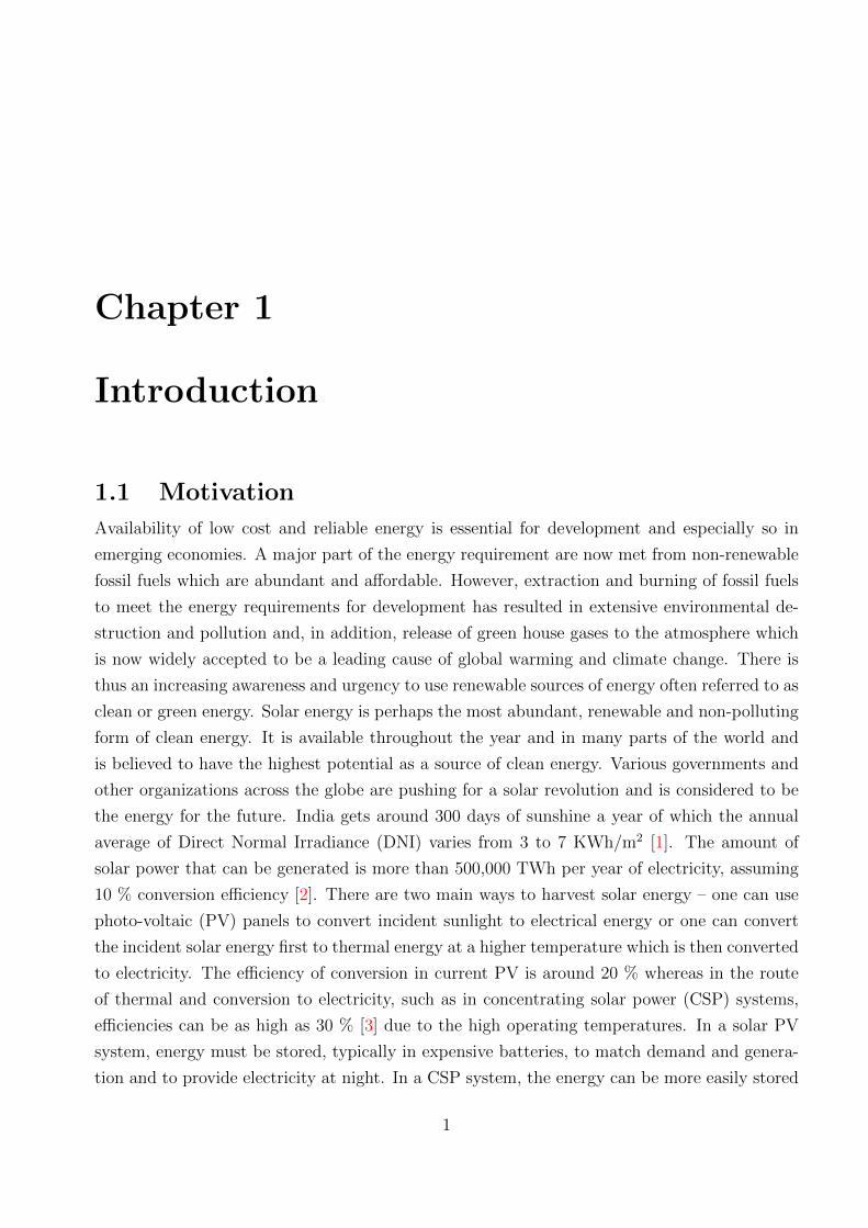
1.1 Motivation
Availability of low cost and reliable energy is essential for development and especially so in
emerging economies. A major part of the energy requirement are now met from non-renewable
fossil fuels which are abundant and affordable. However, extraction and burning of fossil fuels
to meet the energy requirements for development has resulted in extensive environmental de-
struction and pollution and, in addition, release of green house gases to the atmosphere which
is now widely accepted to be a leading cause of global warming and climate change. There is
thus an increasing awareness and urgency to use renewable sources of energy often referred to as
clean or green energy. Solar energy is perhaps the most abundant, renewable and non-polluting
form of clean energy. It is available throughout the year and in many parts of the world and
is believed to have the highest potential as a source of clean energy. Various governments and
other organizations across the globe are pushing for a solar revolution and is considered to be
the energy for the future. India gets around 300 days of sunshine a year of which the annual
average of Direct Normal Irradiance (DNI) varies from 3 to 7 KWh/m2 [1]. The amount of
solar power that can be generated is more than 500,000 TWh per year of electricity, assuming
10 % conversion efficiency [2]. There are two main ways to harvest solar energy – one can use
photo-voltaic (PV) panels to convert incident sunlight to electrical energy or one can convert
the incident solar energy first to thermal energy at a higher temperature which is then converted
to electricity. The efficiency of conversion in current PV is around 20 % whereas in the route
of thermal and conversion to electricity, such as in concentrating solar power (CSP) systems,
efficiencies can be as high as 30 % [3] due to the high operating temperatures. In a solar PV
system, energy must be stored, typically in expensive batteries, to match demand and genera-
tion and to provide electricity at night. In a CSP system, the energy can be more easily stored
1

CHAPTER 1. INTRODUCTION
thermally in molten salts and other medium and electricity can be generated during night or
to match demand. Due to higher efficiency and ease of storage, CSP systems can compete with
solar PV systems and several CSP systems are being developed around the world. One of the
obstacle hindering large scale deployment of CSP plant is the high initial investment required
[4]. In order to bring down the levelised cost of solar electricity, the Sunshot initiative was
launched by the US DoE in 2011. The main goals set for 2020 are to bring solar electricity cost
to $ 0.06 per kWh [5]. Kolb et al. [6], in his work, presents a detailed study of how to improve
technology for reducing the cost. The CSP technology is yet to reach its maturity and it has a
huge potential to be cost effective [7].
In any CSP system, a key task is to concentrate the incident solar energy on to a receiver in
an efficient manner. Typically several mirrors or reflectors are used which reflect the incoming
solar radiation on to a stationary receiver – the mirrors with its support structure, actuators
and controllers is also known as a heliostat. From a large number of heliostats, a large amount
of incident solar energy is concentrated in a small receiver volume resulting in high temperatures
(> 500 ◦C [8]) and this gives rise to higher conversion efficiencies in CSP systems. A typical
solar field could have several thousand such heliostats (for example, at Ivanpah [8] there are
three central receivers and 173500 heliostats) and it is estimated that the heliostats contribute
up to 50 % [9] of the total cost of the CSP system. It is thus an area of research to develop low
cost heliostats.
Generally the Sun moves across the sky daily in an East-West direction and in a North-
South direction with the progress of seasons, a mechanism is needed to track the Sun and reflect
the incident solar energy on to the stationary receiver. Due to the East-West and North-South
motion of the Sun a two axis or a two degree-of-freedom (DOF) mechanism is required for Sun
tracking and reflecting the energy on to the receiver. There exists several two DOF mechanisms
for tracking the Sun (see section 1.4), each having its own advantages and disadvantages. In this
thesis, we propose two parallel manipulators which can be used to track the Sun and thus can
be used as heliostats. We demonstrate that these parallel manipulators have several inherent
advantages over the existing designs and they have the potential to reduce cost and increase
efficiency in CSP systems.
Before we discuss relevant literature on CSP systems and existing Sun tracking system,
in the next section we describe the geometry, the terms and the parameters involved in Sun
tracking.
2
CHAPTER 1. INTRODUCTION
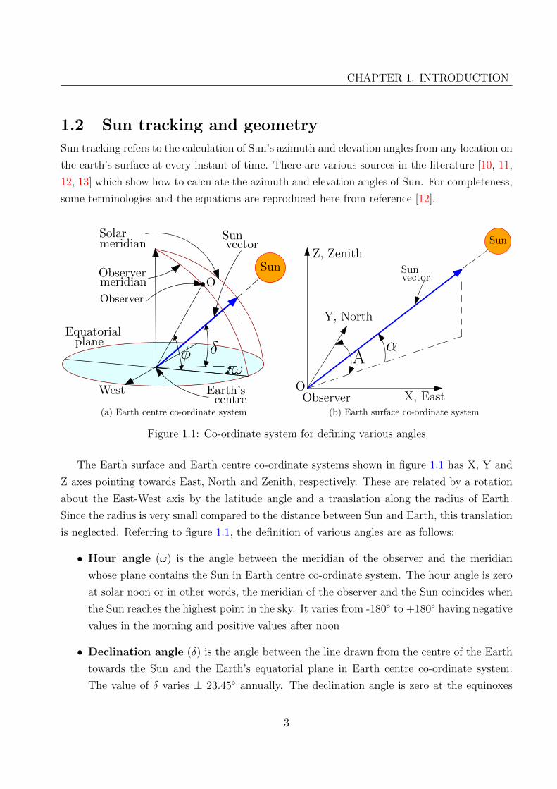
1.2 Sun tracking and geometry
Sun tracking refers to the calculation of Sun’s azimuth and elevation angles from any location on
the earth’s surface at every instant of time. There are various sources in the literature [10, 11,
12, 13] which show how to calculate the azimuth and elevation angles of Sun. For completeness,
some terminologies and the equations are reproduced here from reference [12].
δω
Earth’s
Equatorial
West
Observer
Solar
Sun
centre
Observer
planeφ
meridian
meridian
O
Sunvector
(a) Earth centre co-ordinate system
αA
X, East
Y, North
Z, Zenith
SunSun
ObserverO
Sunvector
(b) Earth surface co-ordinate system
Figure 1.1: Co-ordinate system for defining various angles
The Earth surface and Earth centre co-ordinate systems shown in figure 1.1 has X, Y and
Z axes pointing towards East, North and Zenith, respectively. These are related by a rotation
about the East-West axis by the latitude angle and a translation along the radius of Earth.
Since the radius is very small compared to the distance between Sun and Earth, this translation
is neglected. Referring to figure 1.1, the definition of various angles are as follows:
• Hour angle (ω) is the angle between the meridian of the observer and the meridian
whose plane contains the Sun in Earth centre co-ordinate system. The hour angle is zero
at solar noon or in other words, the meridian of the observer and the Sun coincides when
the Sun reaches the highest point in the sky. It varies from -180◦ to +180◦ having negative
values in the morning and positive values after noon
• Declination angle (δ) is the angle between the line drawn from the centre of the Earth
towards the Sun and the Earth’s equatorial plane in Earth centre co-ordinate system.
The value of δ varies ± 23.45◦ annually. The declination angle is zero at the equinoxes
3
CHAPTER 1. INTRODUCTION
where the day and night are of equal lengths. The declination angle is positive when the
northern part of the earth’s rotational axis is inclined towards the Sun.
• Latitude angle (φ) is the angle between a line drawn from a point on the Earth’s surface
to the center of the Earth and the Earth’s equatorial plane in Earth centre co-ordinate
system. Latitude angle is zero at the equatorial plane and varies between +90◦ at the
North pole to -90◦ at the South pole.
• Azimuth angle (A) is the angle between the local North axis in Earth surface co-ordinate
system and the projection of Sun vector on to the horizontal plane. The azimuth angle
is measured from the local North axis and is positive clockwise. It varies from 0-360◦.
• Elevation angle (α) is the angle the Sun vector makes with the X-Y plane described
in Earth surface co-ordinate system. The elevation angle is zero when the Sun is at the
horizon and varies from 0-90◦
The Sun vector described in Earth surface co-ordinate system has the direction cosines
[cosα sinA cosα cosA sinα]T . Similarly, in Earth centre co-ordinate system, the Sun vector is
[cos δ sinω cos δ cosω sin δ]T . The azimuth and elevation angles are function of the declination,
latitude and hour angle as follows:
α = sin−1(
sin δ sinφ+ cos δ cosω cosφ)
(1.1)
if cosω ≥(
tan δtanφ
),
A = 180− sin−1(− cos δ sinω
cosα
)(1.2)
else if cosω <(
tan δtanφ
),
A = 360 + sin−1(− cos δ sinω
cosα
)(1.3)
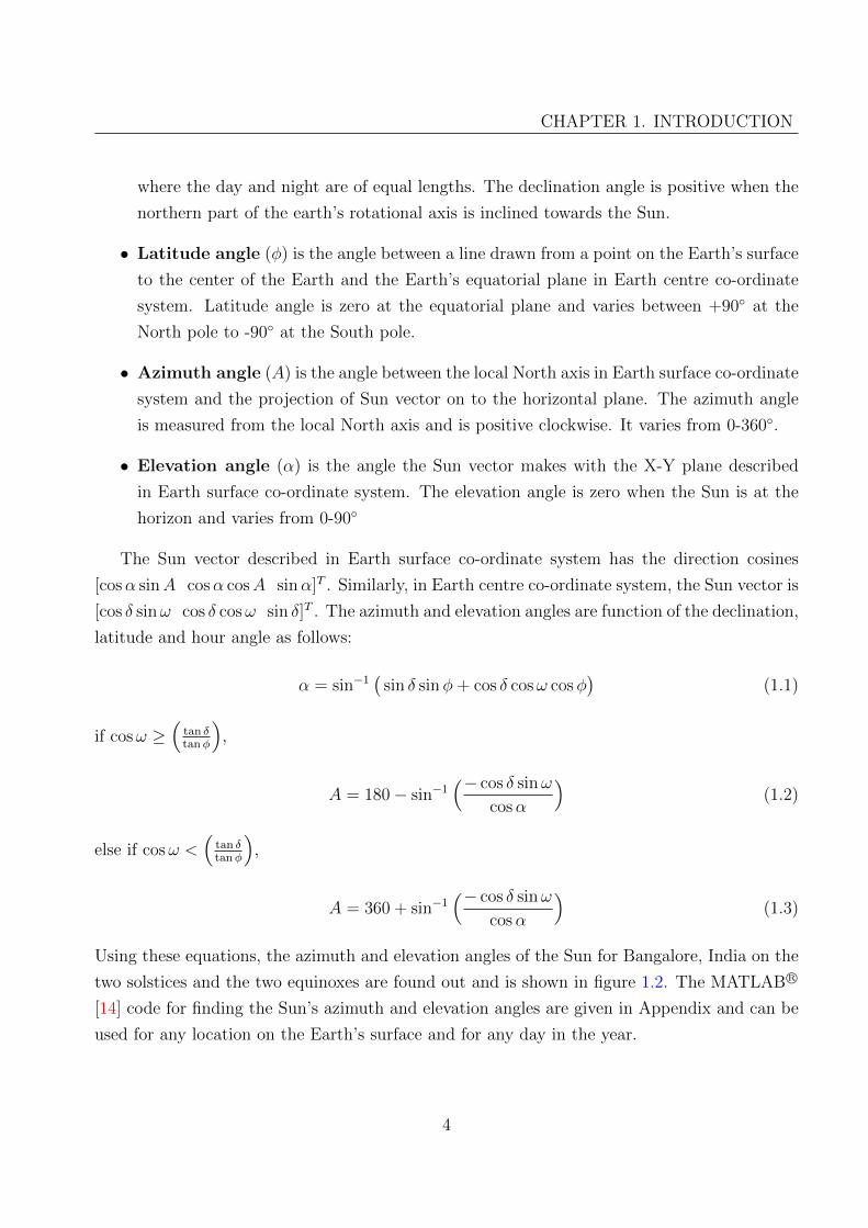
Using these equations, the azimuth and elevation angles of the Sun for Bangalore, India on the
two solstices and the two equinoxes are found out and is shown in figure 1.2. The MATLAB R©
[14] code for finding the Sun’s azimuth and elevation angles are given in Appendix and can be
used for any location on the Earth’s surface and for any day in the year.
4
CHAPTER 1. INTRODUCTION
(a) March equinox (b) June solstice
(c) September equinox (d) December solstice
Figure 1.2: Azimuth and Elevation angles of the Sun for equinoxes and solstices, Bangalore
1.3 Methods for concentrating solar power (CSP)
Solar energy has two parts, namely the direct and diffuse radiations and CSP can only use the
direct radiations. The US Department of Energy (US DoE) gives a comprehensive history of
the solar technology [15]. Energy harvesting from the Sun is classified mainly into two main
categories, viz., concentrating and non-concentrating type. The concentrating type includes
parabolic troughs, paraboloid dishes, central receiver towers, linear Fresnel and Fresnel lenses
(for concentrating photo-voltaic). The non-concentrating type includes flat plate collectors,
evacuated tube and solar ponds. Our primary interest is on concentrating type and in this cat-
egory, the three popular methods are parabolic troughs, paraboloid dishes and central receiver
tower.
1.3.1 Parabolic trough
One of the first persons in the recent history to understand the importance of solar power was
Frank Schuman. He had successfully built a parabolic trough powered water pumping system
in Egypt in 1913 [16]. These troughs track the Sun on one axis and focus the incident solar
5
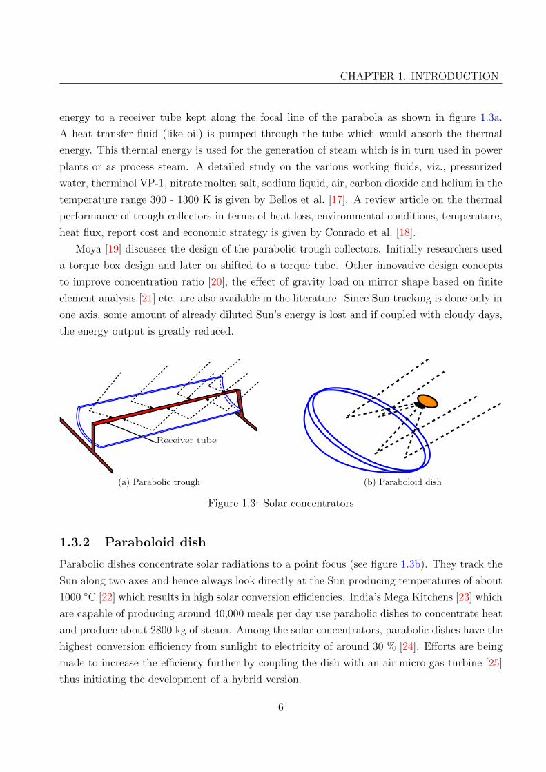
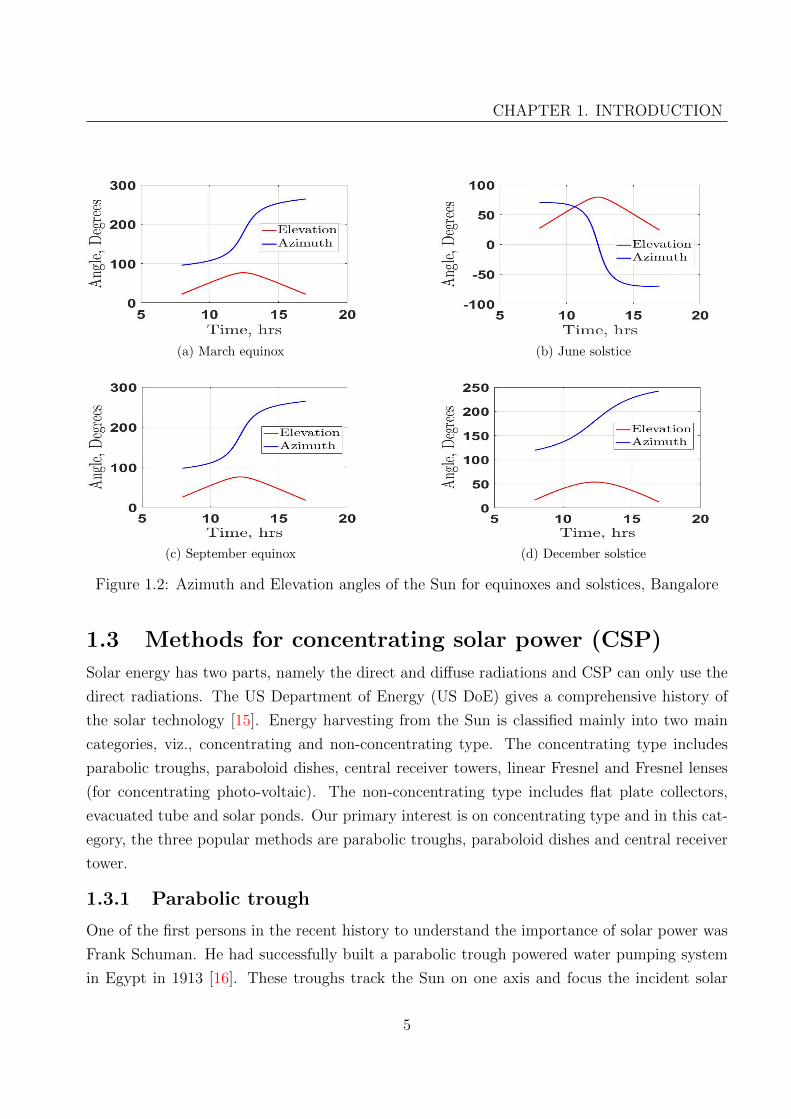
CHAPTER 1. INTRODUCTION
energy to a receiver tube kept along the focal line of the parabola as shown in figure 1.3a.
A heat transfer fluid (like oil) is pumped through the tube which would absorb the thermal
energy. This thermal energy is used for the generation of steam which is in turn used in power
plants or as process steam. A detailed study on the various working fluids, viz., pressurized
water, therminol VP-1, nitrate molten salt, sodium liquid, air, carbon dioxide and helium in the
temperature range 300 - 1300 K is given by Bellos et al. [17]. A review article on the thermal
performance of trough collectors in terms of heat loss, environmental conditions, temperature,
heat flux, report cost and economic strategy is given by Conrado et al. [18].
Moya [19] discusses the design of the parabolic trough collectors. Initially researchers used
a torque box design and later on shifted to a torque tube. Other innovative design concepts
to improve concentration ratio [20], the effect of gravity load on mirror shape based on finite
element analysis [21] etc. are also available in the literature. Since Sun tracking is done only in
one axis, some amount of already diluted Sun’s energy is lost and if coupled with cloudy days,
the energy output is greatly reduced.
Receiver tube
(a) Parabolic trough (b) Paraboloid dish
Figure 1.3: Solar concentrators
1.3.2 Paraboloid dish
Parabolic dishes concentrate solar radiations to a point focus (see figure 1.3b). They track the
Sun along two axes and hence always look directly at the Sun producing temperatures of about
1000 ◦C [22] which results in high solar conversion efficiencies. India’s Mega Kitchens [23] which
are capable of producing around 40,000 meals per day use parabolic dishes to concentrate heat
and produce about 2800 kg of steam. Among the solar concentrators, parabolic dishes have the
highest conversion efficiency from sunlight to electricity of around 30 % [24]. Efforts are being
made to increase the efficiency further by coupling the dish with an air micro gas turbine [25]
thus initiating the development of a hybrid version.
6
CHAPTER 1. INTRODUCTION
Andraka [26] has proposed a thermal energy storage system for the dishes combining latent
energy transport and latent energy storage. In this work, the author investigates the technical
feasibility of the system. Another interesting study by Lertsatitthanakorn et al. [27] attempt
to use a parabolic dish to concentrate Sun’s radiations to a thermoelectric module to generate
electricity.
For both parabolic troughs and paraboloid dishes, precise manufacturing is of utmost im-
portant to achieve the high concentration ratios. Between the two, currently only the parabolic
trough has thermal storage capability of 6 hours [28].
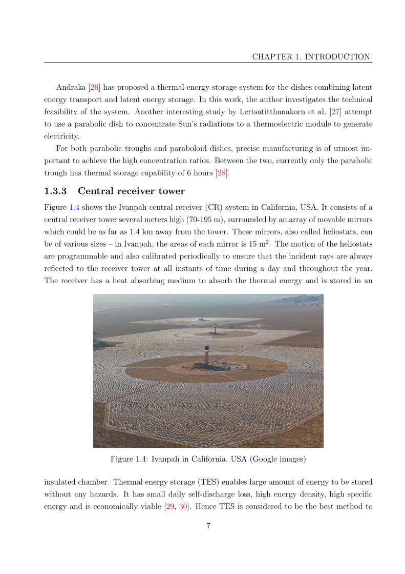
1.3.3 Central receiver tower
Figure 1.4 shows the Ivanpah central receiver (CR) system in California, USA. It consists of a
central receiver tower several meters high (70-195 m), surrounded by an array of movable mirrors
which could be as far as 1.4 km away from the tower. These mirrors, also called heliostats, can
be of various sizes – in Ivanpah, the areas of each mirror is 15 m2. The motion of the heliostats
are programmable and also calibrated periodically to ensure that the incident rays are always
reflected to the receiver tower at all instants of time during a day and throughout the year.
The receiver has a heat absorbing medium to absorb the thermal energy and is stored in an
Figure 1.4: Ivanpah in California, USA (Google images)
insulated chamber. Thermal energy storage (TES) enables large amount of energy to be stored
without any hazards. It has small daily self-discharge loss, high energy density, high specific
energy and is economically viable [29, 30]. Hence TES is considered to be the best method to
7

CHAPTER 1. INTRODUCTION
store energy in CSP plants. TES using phase change materials (PCMs) have been a very active
topic of research in the last two decades or so and several PCMs both organic and inorganic
have been developed. A detailed study of various PCMs are given by Zalba et al. [31] and
Lane [32]. This heat can be used to boil water and generate steam which in turn can be used
to drive a turbine for producing electricity or any other applications which require heat. The
thermal energy stored can also be used for generating process steam for industrial applications
[33]. Latest trends in energy storage may be found in the report published by Sandia National
Laboratories [34].
The first CR demonstration project was carried out in the USA in 1982. This was named
Solar One and had a capacity of 10 MW [15]. The Andasol 1 solar thermal power plant in
Andalucia, Spain, [35] claims that they can produce electricity from heat stored in molten salts
(28500 tons) for seven and a half hours after sunset. The receiver outlet temperature achieved
in CR systems is very high (about 565 0C in Ivanpah, USA) and hence this heat could be used
at night to drive a steam turbine. The high temperature achieved also helps in achieving higher
conversion efficiencies as per the Carnot’s theorem [36].
1.4 Overview of existing Sun tracking methods
There are various algorithms used for Sun tracking (see Lipps and Vant-Hull [37]) – the main
ones are the azimuth-elevation, radial-pitch-roll, azimuthal-pitch-roll, polar and the target-
aligned. Mousazadeh et al. [38] and Lee et al. [39] present a review of the Sun-tracking methods
employed currently by various researchers across the globe using passive, single-axis and dual
axis tracking. This paper also gives the energy gain obtained while using various types of
trackers, close-loop and open-loop types of tracking employed currently. The most popular
method for tracking the Sun in central receiver systems is the Azimuth-Elevation (Az-El) . The
Target-Aligned (T-A) or also called as the spinning-elevation method is also developed as an
alternate tracking methodology but almost not used at all. In both the above methods, there
are two actuators which track the Sun and orient the heliostats in such a way that the incident
ray from the Sun is always reflected onto a fixed central receiver.
As mentioned in section 1.2, the relative motion of the Sun in the sky with respect to Earth
is known completely from the knowledge of date, time and location. Referring to figure 1.5, let
O represents the origin of the global co-ordinate system (which is also the base of the receiver
tower) and the OX, OY and OZ axes pointing towards the East, North and Zenith directions
respectively. Let the mirror centre be at G and−−→GN,
−→GR and
−→GS denote the unit vectors
representing the normal to the mirror, reflected ray and Sun-vector, respectively. From the
laws of reflection, a) the incident ray, reflected ray and the normal should lie on the same plane,
8
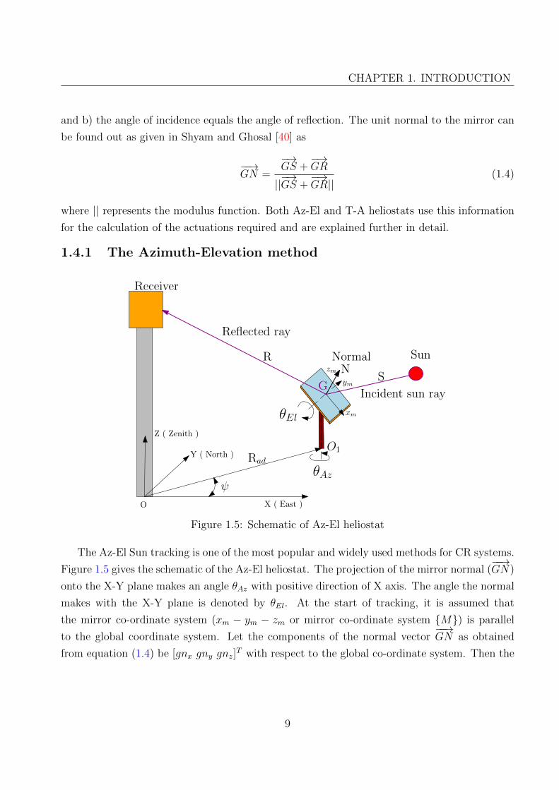
CHAPTER 1. INTRODUCTION
and b) the angle of incidence equals the angle of reflection. The unit normal to the mirror can
be found out as given in Shyam and Ghosal [40] as
−−→GN =
−→GS +
−→GR
||−→GS +−→GR||
(1.4)
where || represents the modulus function. Both Az-El and T-A heliostats use this information
for the calculation of the actuations required and are explained further in detail.
1.4.1 The Azimuth-Elevation method
θAz
θEl
X ( East )
Y ( North )
Z ( Zenith )
O
Receiver
Reflected ray
Normal
Incident sun rayG
Sun
S
R
O1
ψ
Rad
N
xm
ym
zm
Figure 1.5: Schematic of Az-El heliostat
The Az-El Sun tracking is one of the most popular and widely used methods for CR systems.
Figure 1.5 gives the schematic of the Az-El heliostat. The projection of the mirror normal (−−→GN)
onto the X-Y plane makes an angle θAz with positive direction of X axis. The angle the normal
makes with the X-Y plane is denoted by θEl. At the start of tracking, it is assumed that
the mirror co-ordinate system (xm − ym − zm or mirror co-ordinate system {M}) is parallel
to the global coordinate system. Let the components of the normal vector−−→GN as obtained
from equation (1.4) be [gnx gny gnz]T with respect to the global co-ordinate system. Then the
9
CHAPTER 1. INTRODUCTION
actuations required can be found out as a function of time as
θAz = arctan
(gnygnx
)(1.5)
θEl = arctan
(gnz√
gn2x + gn2
y
)(1.6)
The Az-El can also be used for all other types of solar energy harvesting techniques including
CR systems, parabolic troughs and dishes. Though simple and economical, the Az-El method
of tracking has numerous disadvantages [22]. In order to overcome the short comings of the
Az-El method, another method of tracking called the target-aligned method was proposed and
is described next.
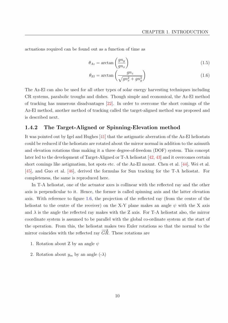
1.4.2 The Target-Aligned or Spinning-Elevation method
It was pointed out by Igel and Hughes [41] that the astigmatic aberration of the Az-El heliostats
could be reduced if the heliostats are rotated about the mirror normal in addition to the azimuth
and elevation rotations thus making it a three degree-of-freedom (DOF) system. This concept
later led to the development of Target-Aligned or T-A heliostat [42, 43] and it overcomes certain
short comings like astigmatism, hot spots etc. of the Az-El mount. Chen et al. [44], Wei et al.
[45], and Guo et al. [46], derived the formulas for Sun tracking for the T-A heliostat. For
completeness, the same is reproduced here.
In T-A heliostat, one of the actuator axes is collinear with the reflected ray and the other
axis is perpendicular to it. Hence, the former is called spinning axis and the latter elevation
axis. With reference to figure 1.6, the projection of the reflected ray (from the centre of the
heliostat to the centre of the receiver) on the X-Y plane makes an angle ψ with the X axis
and λ is the angle the reflected ray makes with the Z axis. For T-A heliostat also, the mirror
coordinate system is assumed to be parallel with the global co-ordinate system at the start of
the operation. From this, the heliostat makes two Euler rotations so that the normal to the
mirror coincides with the reflected ray−→GR. These rotations are
1. Rotation about Z by an angle ψ
2. Rotation about ym by an angle (-λ)
10

CHAPTER 1. INTRODUCTION
θsp
θel
X ( East )
Y ( North )
Z ( Zenith )
O
ψ
Rλ
Receiver
Sun
Reflected ray
Incident
G
SNormal sun ray
O1Rad
N
ym
xmzm
Figure 1.6: Schematic of the Target-Aligned heliostat
and the resultant rotation matrix is given by
R12 =
cos (ψ) cos (λ) − sin (ψ) − cos (ψ) sin (λ)
sin (ψ) cos (λ) cos (ψ) − sin (ψ) sin (λ)
sin (λ) 0 cos (λ)
(1.7)
After the first two rotations, the heliostat rotates about−→GR by an angle θsp (spinning angle)
so that the the reflected ray, mirror normal (−−→GN) and the xm axis of the mirror co-ordinate
system become coplanar. Then finally, it rotates about an axis (ym) which is perpendicular to−→GR in the plane of the mirror by an angle θel where θel is the half angle between the incident
and reflected rays. The spinning and elevation angles can be found out as a function of time as
θsp = arctan
(−−→GP0 × (
−→GS .
−→GR)
−−→GP0 .
−→GS
)(1.8)
θel = 0.5 arccos(−→GS .
−→GR) (1.9)
where−−→GP0 is the vector given by the first column of the matrix R12.
The T-A method is exclusively designed for CR systems. Although, the T-A was developed
to overcome the short comings of the Az-El method, in a comparative study of Az-El and T-A
11

CHAPTER 1. INTRODUCTION
heliostats by Chen et al. [47], it is shown that for certain times of the day and year, Az-El
performs better then T-A in terms of spillage losses and concentration.
1.4.3 Limitations of Az-El and T-A methods
As shown in figures 1.5 and 1.6, the mirrors are supported by a support frame and a pedestal
which is fixed to the ground. The pedestal with the drives for the Az-El and the T-A heliostats
are typically placed at the geometrical center of the mirror assembly. Due to this arrangement,
the deflection of the support frame and the mirrors due to self-weight and wind load can go
beyond the allowable slope error limit of 2 - 3 mrad [22] at the edges or corner of the mirror
structure. In a heliostat field, the distance of the farthest mirror could be as more than 1.4 km.
Thus the reflected ray from the mirror may not hit the receiver aperture. In order to tackle
this problem, either the support frame has to be made more rigid or smaller sized heliostats
have to be used.
To increase the concentration of incident solar radiation, the mirrors in a heliostat are typi-
cally canted – the arrangement of mirrors such that it approximate a paraboloid of revolution.
There are different types of canting methods like on-axis, off-axis and parabolic canting. A
comprehensive study of these methods has been made by Buck and Teufel [48]. Even though
canting gives a better concentration ratio, it effectively modifies the focal point and introduces
what is called the off-axis aberration as reported by Rabl [49].
The relative motion of Sun with respect to Earth is very slow – the Sun roughly goes
East-West and traverses approximately 180◦ in about 12 hours or about 15◦ per hour. A
simple computation shows that the rotation speed of the heliostat should be of the order of
7×10⁻⁵ rad/s. If typical DC electric motors, at 10 rpm, is used, it can be shown that large gear
reductions (of the order of 1:15000) need to be used to track the Sun for both the Az-El and
T-A methods of tracking. Gear boxes with such large reductions are expensive and typically
introduce large friction and backlash errors which in turn makes Sun tracking inaccurate. To
avoid large gear reductions, intermittent tracking is often used.
In order to avoid some of these difficulties, researchers have developed tracking strategies
using linear actuators. An exciting tracking methodology is the pitch-roll or tip-tilt using two
linear actuators. Lindberg and Maki [50] gives a detailed account of the stress analysis in
presence of gravity and wind for the pitch-roll heliostat and a complete vector-based inverse
kinematic solution of the pitch-roll heliostat was provided by Freeman et.al. [51]. One of the
main advantages of such a system over the Az-El is that it uses less ground space. The Stellio
heliostat [52, 53] uses two linear actuators in what is called a slope-drive configuration. This
type of drive eliminates the high velocity required for large change in azimuth especially when
12

CHAPTER 1. INTRODUCTION
the heliostat normal reaches the vertical. Such a drive cannot be used for all heliostats in the
field due to mechanical restrictions and the maximum angular distance that it can traverse is
around 110◦.
1.5 Errors sources and its control
There are various sources of tracking errors [54, 55] which eventually decrease the annual output
of the CSP plants. They can be categorized into two main groups – optical and tracking error.
The optical error can further be divided into slope and specular error. The macroscopic shape
or the non-flatness of mirror due to manufacturing errors contributes to the slope error whereas
the microscopic roughness causes the specular error. The tracking error occurs due to the errors
in the control system. It is estimated that the sum of all these three sources of errors should
be about 5 - 6 mrad for acceptable performance of a heliostat. In addition, the error from each
of the sources are often apportioned as maximum optical error of less than 3 and 4 mrad [56]
during calm and windy conditions respectively and maximum tracking error due to control of
2 mrad [57]. Reducing specular error is difficult and leads to increased cost. The error due to
wind loading and self-weight can be reduced by appropriate design. The errors in tracking are
due to reasons such as errors in modeling the motion of the Sun and inaccuracies in setting
or measurement of co-ordinates of the heliostats, backlash in gears used in the drive system
and errors in feedback from the joint encoders. Jones and Stone [58] analyze the tracking error
sources in Solar Two CR system in Mojave desert, California. They have come up with a novel
’move’ strategy to minimize tracking error by accurately surveying and storing in database.
Various other researchers such as Stone and Kiefer [59], Malan and Gauche [60], and Kribus
et al. [61] have tried to improve the tracking accuracy using open loop, model based and closed
loop control strategies, respectively. Another closed loop control strategy for T-A heliostats was
developed by Roos et al. [62] which ensures a tracking accuracy of 3.3 mrad. Even though closed
loop tracking algorithms are available, their rather tedious task of installing CCD cameras has
forced the current industrial norm to be of open loop tracking. This is achieved by a periodic
calibration using a target screen situated below the receiver aperture and image processing
techniques (see figure 1.7 [63]). The heliostats on the field reflect the incident Sun rays on
to the calibration target one by one. There would be a camera to observe the target and a
central control system which would be already fed with each heliostat parameters and the shift
required to move the incident beam from the calibration target to the receiver aperture. The
main disadvantage of this method is that only one heliostat could be calibrated at a time.
13

CHAPTER 1. INTRODUCTION
Figure 1.7: Calibration target for open-loop tracking
1.6 Contributions of the thesis
The focal point of this thesis is towards analysis and design of mechanisms which can help in
development of low cost heliostats. The main contributions of the thesis are in the area of use
of parallel manipulators for heliostats. Specifically the contributions of this work are as follows:
• Two three-DOF parallel manipulators to track the Sun. The 3-RPS parallel manipulator
is shown to have less spillage losses as compared to existing Az-El and T-A mechanisms.
A 3-UPU wrist manipulator which can be used in the Az-El or in the T-A configuration
has also been proposed.
• The kinematic equations for the 3-RPS and the 3-UPU wrist parallel manipulators to
track Sun in CR systems are developed. Extensive simulation study has been conducted
to find out the actuations required, range of motion of the rotary and spherical joints
used in the mechanisms and intersection of the legs with each other.
• Design of the mirror support structure for wind and gravity loading satisfying a slope
error criteria of 2 mrad using finite element analysis has been carried out. It is shown
that the use of the parallel manipulators can reduce the weight of the structure by 15 -
60 % for small to large heliostats, respectively.
• For the 3-RPS parallel manipulator based heliostat, extensive simulations have been done
to obtain optimized design parameters. It is shown that the stroke required for the
actuators is less than 700 mm for a 2 m x 2 m heliostat placed 300 m away from the
receiver tower in Bangalore.
14

CHAPTER 1. INTRODUCTION
• A prototype of the 3-RPS heliostat with a mirror of dimension of 1 m x 1 m has been
manufactured. The control algorithm and the developed control system is used to move
the heliostat and Sun tracking is demonstrated.
• The tracking error is quantified and it is shown that the prototyped Az-El and 3-RPS
based heliostats have comparable tracking errors of 20 mrad and 30 mrad respectively.
1.7 Preview
The organization of the thesis is as follows:
In chapter 2, two main aspects, viz., the existing Sun tracking using parallel manipulators
and kinematics and simulation study of the proposed 3-RPS and 3-UPU wrist have been done.
Chapter 3 gives a description of the finite element analysis done to find the least weight support
structure. This chapter also provides an iterative approach to find certain design variables for
minimizing the stroke of actuators and static and dynamic analysis of the 3-RPS heliostat.
Chapter 4 provides the details regarding the prototype design, control strategy and the actual
experimental validation. Finally, chapter 5 provides the conclusions and future directions of
the work.
15
Chapter 2
Sun tracking using parallel
manipulators
2.1 Introduction
The traditional Azimuth-Elevation (Az-El) and the Target-Aligned (T-A) arrangements are
kinematically in a serial configuration where the actuators are placed one after the other. The
mirror is also essentially mounted at a point after the two actuators used in these configuration.
As in any serial configuration, the pointing or tracking error in the arrangement is the sum of
the errors of the two actuators and due to the point support, the deflection in the mirror due to
wind and self-weight is similar to that of a cantilever. In order to keep the pointing and tracking
error within the allowable limit of 2 - 3 mrad, accurate and expensive drives with gear reduction
is used and to overcome deflection due to loading, stiff and heavy supporting structures are
used or smaller heliostats need to be used. Smaller heliostats implies that a large number of
heliostats are required for a required power output from the solar plant with each heliostat
containing two actuators with expensive drives. From the time the parallel manipulators were
first introduced by Gough [64] and Stewart [65], it has been known that parallel manipulators
provide high structural rigidity and more accurate positioning and orientation of the end-effector
or the moving platform [66].The increased rigidity is due to the fact that the moving platform
is supported at multiple points thereby the external load is shared. The increased accuracy
is due to the fact that the positioning and pointing error of the end-effector is a function of
the largest error in any actuator and not the sum of the errors as in a serial arrangement.
Due to these inherent advantages, parallel manipulators have been extensively used in flight
simulators, precision manufacturing, pointing devices, medical applications, and, more recently,
in video games. Since precise positioning of the end-effector (mirror in our case) is one of the
16
CHAPTER 2. SUN TRACKING USING PARALLEL MANIPULATORS
advantages, use of a parallel manipulator can lead to use of low cost actuators and drives. With
the increased rigidity, a heliostat can be designed with larger mirrors or for smaller mirrors,
the supporting material required to withstand wind loading can be less. For a required power
output from a solar plant, larger mirrors in each heliostat implies less number of heliostats and
less number of actuators required in the field and less supporting material results in lowering of
material and fabrication cost of a heliostat. Hence, a parallel manipulator is expected to lead
to cost savings in concentrated solar power systems.
In this chapter, two 3-DOF parallel manipulators, viz., the 3-UPU wrist and 3-RPS parallel
manipulator are proposed to be potential candidates for Sun tracking in central receiver systems.
The ‘U’ denotes a two-DOF Hooke joint, the ‘P’ denotes single DOF a prismatic or a sliding
joint, ‘R’ denotes a one-DOF revolute or a rotary joint and ‘S’ denotes a three-DOF spherical
joint. In both these parallel manipulators, the ‘P’ joint is actuated and the other joints are
not actuated or are passive. The 3-UPU wrist can be operated in both the Az-El and T-A
mode by simply changing software and control strategy and does not require any change in the
hardware. The 3-UPU wrist can thus be operated in a mode which gives the best performance
in terms of spillage losses or astigmatism at a particular time of the day or a date in the year.
The 3-RPS configuration has other inherent advantages when compared to the Az-El and T-A
methods and these are discussed in detail in this chapter. In both the parallel configurations,
linear actuators are used. The motion of the prismatic (P) joints or the stroke of the linear
actuators are computed using simple inverse kinematics algorithms and adjusted with respect
to time to achieve the orientation required for Sun tracking. The two parallel manipulators
require three actuators as opposed to two in the Az-El and T-A configurations. However, since
the support material is less or larger mirrors can be used and less expensive and less accurate
linear actuators can be used, the overall cost of the plant is expected to be less.
The chapter is organized as follows: Section 2.2 gives an overview of the existing approaches
for Sun tracking using parallel manipulators. In section 2.3, a detailed description of the 3-
RPS parallel manipulator’s geometry, inverse kinematics equations, modeling of R-P-S leg and
spherical joint and simulations results are given. In section 2.4, the kinematics of the 3-UPU
wrist manipulator and the simulation results and observations made during the simulation
study are presented. Finally section 2.6 presents the conclusions and challenges ahead.
17
CHAPTER 2. SUN TRACKING USING PARALLEL MANIPULATORS
2.2 Overview of existing Sun tracking methods using
parallel manipulators
There have been a few attempts to use parallel manipulators in Sun tracking for concentrated
solar power systems. We present these attempts and their shortcomings.
2.2.1 The U-2PUS parallel manipulator and the CAPAMAN
In the work by Cammarata [67], a two degree-of-freedom parallel manipulator called the U-2PUS
has been developed for photo-voltaic (PV) systems. The author claims that this manipulator
is ideal for photo-voltaic systems in latitudes from 0 to 500. This parallel manipulator could
be used for photo-voltaic systems but cannot be used for CR systems since in a field with
photo-voltaic panels, all the PV panels are tracked in a similar manner. There is no reflection
of the incident solar radiation and the conversion to electricity takes place in the PV panel
itself. The location of the PV panels in the field do not play any part as the Sun’s rays are
parallel everywhere. For central receiver systems, the heliostats at different locations in the
field will have different motion if the incident energy is to be reflected to a central receiver.
Mathematically, it can be shown that there are more unknowns than equations available in the
U-2PUS parallel manipulator system and hence it cannot be used in a CR system.
A three-degree-of-freedom parallel manipulator called CAPAMAN, containing a 17 links and
18 joints, has also been proposed for sun tracking [68]. However, to the best of our knowledge,
there are no experimental results available in literature.
2.2.2 Other parallel mechanisms
A four degree-of-freedom parallel manipulator is proposed for Sun-tracking by Altuzarra et al.
[69]. In his work, the collector initially is kept (before the tracking starts) high above the
ground and by letting it fall in a controlled manner (using four sliders attached to it under
the influence of gravity), the required orientation is achieved. This mechanism casts its own
shadow on the collector. Although simulation results appear to be good, no prototype has been
made and tested. To make the mechanism stiffer, some redundant bars are also used.
Google Inc. [70, 71] also developed a novel method for changing the position and orientation
of the reflector (mirror). They proposed the use of an electric cable drive system which is
constantly under tension. They also claim that this method will reduce the power consumption,
size and cost of the actuator system. However, their light-weight frame design is susceptible to
gusty winds and could be used only at places where wind velocities are very low.
Several other 2-DOF spherical mechanisms [72, 73, 74, 75] for application specific purposes
18
CHAPTER 2. SUN TRACKING USING PARALLEL MANIPULATORS
such as camera orientation, scanning spherically shaped items etc. are described in literature
but none of these have been shown to be capable of tracking Sun for a central receiver systems.
Thus it is clear that the current Sun tracking approaches suffer from serious shortcomings
be it large tracking errors as in the case of serial mechanisms to the inability to find the various
orientations required for tracking for CR systems in parallel mechanisms. In this chapter the
focus is on CR systems and we propose two potential parallel manipulators, viz., the 3-UPU
wrist and the 3-RPS parallel manipulator that can be used for tracking without any of the
above mentioned disadvantages. In addition, the 3-UPU can be reconfigured to be used either
in Az-El or in the T-A method thus combining the advantages of both. From the next section
onwards, the detailed study on the 3-RPS and the 3-UPU wrist parallel manipulators are carried
out to investigate the merits of using them in CR systems.
2.3 Geometry and kinematics of a 3-RPS manipulator
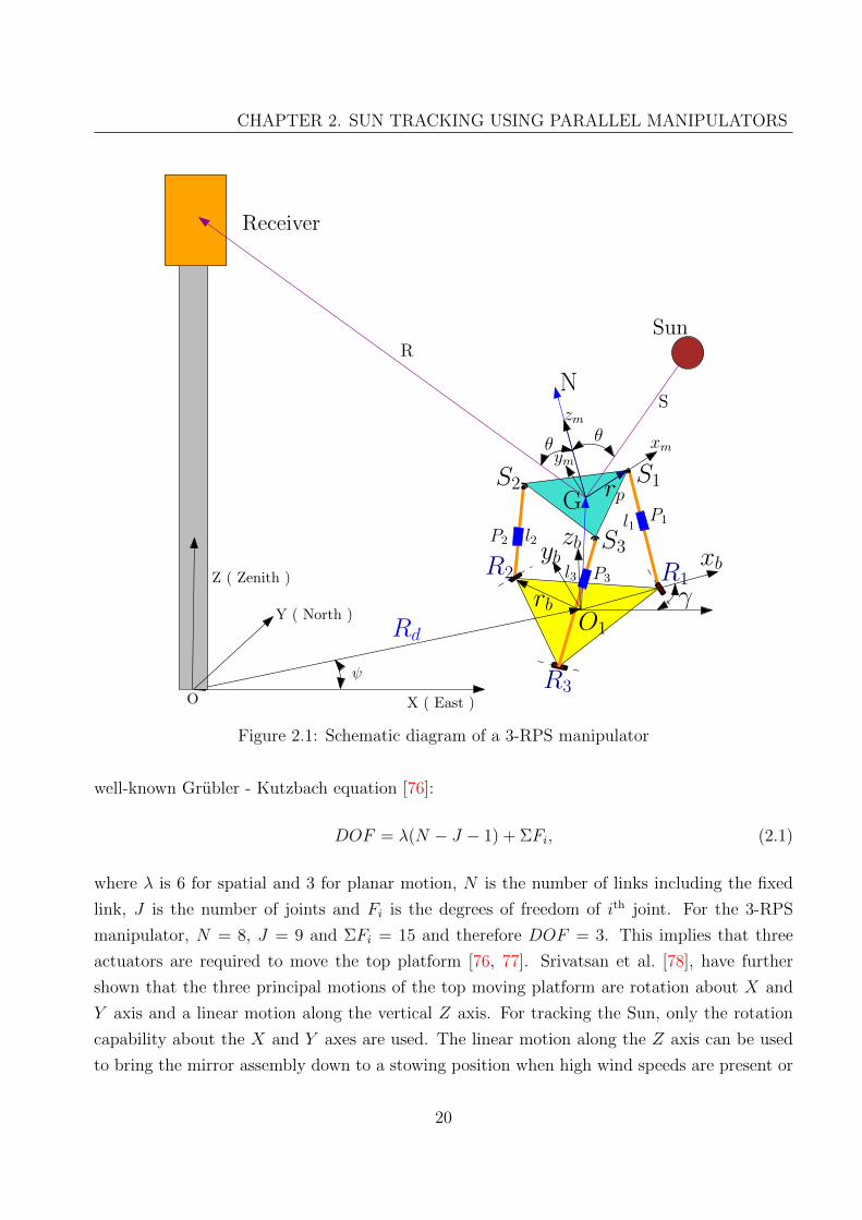
Figure 2.1 shows the well known three-degree-of-freedom 3-RPS parallel manipulator. It con-
sists of a moving top platform which is connected to a fixed base by means of three actuated
prismatic(P) joints Pi, (i=1, 2, 3). At each of the connection points, Si, (i = 1, 2, 3), at the
moving top platform, there is a spherical (S) joint and at each of the connection points at the
fixed base, Ri, (i = 1, 2, 3), there is a rotary (R) joint. The axes of the rotary joints are in
the plane of the fixed platform. The mirror assembly is fixed to the top moving platform using
a support structure (as shown in figure 2.2) which is designed to provide adequate stiffness
such that deflections due to wind loads and self-weight are within acceptable limits. Referring
to figure 2.1, the foot of the receiver tower and the origin, O, of the fixed coordinate system
coincides with each other. The point O1 is at a distance, Rd, from O and at an angle ψ with
respect to the OX axis. The co-ordinate system at O1 with axis {xb, yb, zb} (base coordinate
system, {B}) is described with respect to the fixed coordinate system by a rotation γ about Z
axis and a translation along−−→OO1. The coordinate system at G is denoted with {xm, ym, zm}
(mirror coordinate system {M}) and the vector−−→O1G is denoted by [xG, yG, zG]T with respect to
{B}. The variables l1, l2 and l3 are the actuations at the prismatic joints and are functions of
azimuth and elevation angles of Sun, heliostat location in the field, height of the receiver tower
and the distance of the connection points from the centre. Even though the mirror assembly
can have arbitrary shapes, for the purpose of kinematics, only the triangle formed by Ri’s and
Si’s need to be considered where i = 1, 2, 3. Without loss of generality, it is assumed that
the triangle formed by the Ri’s and Si’s form an equilateral triangle whose circum-radius is rb
and rp respectively. The degrees of freedom of the manipulator can be found out by using the
19
CHAPTER 2. SUN TRACKING USING PARALLEL MANIPULATORS
P1
P2
P3
xbybzb
G
SN
θθ
rp
R1R2
R3
S1S2
S3
γ
xmym
zm
Rd
l1l2
l3
O1
rb
X ( East )
Y ( North )
Z ( Zenith )
O
ψ
R
Receiver
Sun
Figure 2.1: Schematic diagram of a 3-RPS manipulator
well-known Grubler - Kutzbach equation [76]:
DOF = λ(N − J − 1) + ΣFi, (2.1)
where λ is 6 for spatial and 3 for planar motion, N is the number of links including the fixed
link, J is the number of joints and Fi is the degrees of freedom of ith joint. For the 3-RPS
manipulator, N = 8, J = 9 and ΣFi = 15 and therefore DOF = 3. This implies that three
actuators are required to move the top platform [76, 77]. Srivatsan et al. [78], have further
shown that the three principal motions of the top moving platform are rotation about X and
Y axis and a linear motion along the vertical Z axis. For tracking the Sun, only the rotation
capability about the X and Y axes are used. The linear motion along the Z axis can be used
to bring the mirror assembly down to a stowing position when high wind speeds are present or
20

CHAPTER 2. SUN TRACKING USING PARALLEL MANIPULATORS
Figure 2.2: CAD model of the 3-RPS manipulator
for optimization.
The homogeneous transformation matrix [T ] which relates the coordinate system at O1 and
G can be described
[T ] =
n1 o1 a1 xG
n2 o2 a2 yG
n3 o3 a3 zG
0 0 0 1
(2.2)
where xG, yG and zG are the co-ordinates of a reference point, G, on the top platform (fixed
to the mirror), (n1, n2, n3)T , (o1, o2, o3)
T and (a1, a2, a3)T denote the direction cosines of the
xm, ym and normal (zm) axes of the mirror co-ordinate system with respect to the base.
2.3.1 Kinematics of a 3-RPS manipulator
In the kinematics of a parallel manipulator, there are two well-known problems. In the direct
kinematics problem, the prismatic joint variables l1, l2 and l3 are known and the position vector
(xG, yG, zG)T of a reference point on the moving platform, G, and the orientation of the top
platform or the 4×4 homogeneous transformation matrix [T ] are to be found out. In the inverse
kinematics problem, for a given [T ], the prismatic joint variables need to be obtained. For Sun
tracking, we are primarily interested in the inverse kinematics of the manipulator.
21
CHAPTER 2. SUN TRACKING USING PARALLEL MANIPULATORS
In the inverse kinematics of 3-RPS manipulator, the elements of the transformation ma-
trix, (equation (2.2)), can be computed from the knowledge of Sun vector, the location of the
central receiver tower and the heliostats in a field and the three geometrical constraints of the
manipulator itself. As the Sun moves in the sky, the elements of the transformation matrix
change with time and at each instant the leg lengths, li, i = 1, 2, 3 of the manipulator need
to be calculated. Since the 3-RPS manipulator has three degrees-of-freedom and the tracking
of the Sun requires only two variables, there are several constraint equations relating the 12
unknowns in the transformation matrix [T ]. As mentioned earlier, the rotation about the X
and Y axis are used for orienting the top platform and one can choose the vertical motion of
the top platform, zG arbitrarily. To obtain the other constraints we proceed as follows.
As for any transformation matrix, we can write five constraint equations as
n21 + n2
2 + n23 = 1
o21 + o22 + o23 = 1
n1a1 + n2a2 + n3a3 = 0
n1o1 + n2o2 + n3o3 = 0
o1a1 + o2a2 + o3a3 = 0 (2.3)
where (n1, n2, n3)T , (o1, o2, o3)
T and (a1, a2, a3)T are from equation (2.2).
The normal to the mirror,−−→GN , is given by equation (1.4). From prior knowledge of the
receiver co-ordinates, it can be found that the reflected ray−→GR is a function of xG, yG and the
assumed value of zG. Since−→GS is known in terms of azimuth and elevation angles of the Sun,
the normal−−→GN is also a function of the azimuth and elevation angles of the Sun and xG, yG
and the assumed value of zG. This implies that the direction cosines a1, a2 and a3 of the normal
vector−−→GN are functions of five variables of which xG and yG are the unknowns.
The 3-RPS configuration introduces additional three constraints [77] given by
yG + n2rp = 0 (2.4)
n2 = o1 (2.5)
xG =rp2
(n1 − o2) (2.6)
where rp is the circum-radius of the top equilateral triangle. Thus there are 8 equations in 8
22
CHAPTER 2. SUN TRACKING USING PARALLEL MANIPULATORS
unknowns, {xG, yG, n1, n2, n3, o1, o2, o3}. From equations (2.4) and (2.5),
n2 = o1 =−yGrp
and from equation (2.6),
o2 = n1 −2xGrp
Eliminating n2, o1 and o2, we get
n21 + (
yGrp
)2 + n23 = 1 (2.7)
(yGrp
)2 + (n1 −2xGrp
)2 + o23 = 1 (2.8)
n1a1 −yGrpa2 + n3a3 = 0 (2.9)
−2n1yGr
+2xGyGr2p
+ n3o3 = 0 (2.10)
−yGrp
a1 + (n1 −2xGrp
)a2 + o3a3 = 0 (2.11)
Thus we arrive at 5 equations in 5 unknowns, i.e., (n1, n3, o3, xG and yG) which can be further
reduced by substitution and using Bezout’s method of elimination [79]. Finally we get two
equations in xG and yG given in equations (2.12) and (2.13) below. Equations (2.12) and (2.13)
are numerically solved for xG and yG in MATLAB R© using the inbuilt routine fsolve for a given
a1, a2 and a3. The two equations are as follows:.
d1x2G + e1xG + f1 = 0, (2.12)
d2x2G + e2xG + f2 = 0, (2.13)
d1 = −12yG
2a22
a12rp4− 4
yG2
rp4− 4
yG2a2
4
a14rp4+ 4
a22
rp2a32− 4
yG2a2
4
rp4a32a12+ 4
a22
a12rp2− 8
a32yG
2a22
a14rp4
− 4yG
2a22
rp4a32− 4
a34yG
2
a14rp4− 8
a32yG
2
a12rp4
e1 = −4a1yG
3a2rp4a32
− 4a2
5yGa13a32rp2
+ 4yGa2
3
rp2a1a32− 4
a32yGa2a13rp2
+ 4yG
3a25
rp4a13a32− 8
yGa23
a13rp2− 4
yG3a2
rp4a1
+ 4yG
3a23
rp4a13
23
CHAPTER 2. SUN TRACKING USING PARALLEL MANIPULATORS
f1 =yG
2
rp2− 5
yG4a2
4
rp4a14− a2
2
a12+
yG4a2
4
rp4a12a32+
a26yG
2
a14a32rp2+ 4
a34yG
2
a14rp2− 4
a34yG
4
rp4a14+ 4
a32yG
2
a12rp2
− 8a3
2yG4
rp4a12− 5
yG4
rp4− a1
2yG4
rp4a32− 6
yG4a2
2
rp4a12+ 8
a32yG
2a22
a14rp2− 8
yG4a3
2a22
rp4a14+yG
4a22
rp4a32
+ 5yG
2a24
a14rp2− 2
yG2a2
4
rp2a12a32+ 2
yG2a2
2
a12rp2+yG
2a22
rp2a32− yG
4a26
rp4a14a32
d2 = −4a3
4yG2
a14rp4− 4
a24yG
2
a14rp4− 4
a24yG
2
rp4a32a12+ 4
a24
rp2a12a32− 8
a32yG
2
a12rp4+ 4
a22
rp2a12
− 8a3
2a22yG
2
a14rp4− 4
a22yG
2
rp4a32− 12
a22yG
2
a12rp4− 4
yG2
rp4
e2 = −4a1yG
3a2rp4a32
− 4a2
5yGa13a32rp2
+ 4yGa2
3
rp2a1a32− 4
a32yGa2a13rp2
+ 4yG
3a25
rp4a13a32− 8
yGa23
a13rp2
− 4yG
3a2rp4a1
+ 4yG
3a23
rp4a13
f2 =yG
2
rp2− 5
yG4a2
4
rp4a14− a2
2
a12+
yG4a2
4
rp4a12a32+
a26yG
2
a14a32rp2+ 4
a34yG
2
a14rp2− 4
a34yG
4
rp4a14+ 4
a32yG
2
a12rp2
− 8a3
2yG4
rp4a12− 5
yG4
rp4− a1
2yG4
rp4a32− 6
yG4a2
2
rp4a12+ 8
a32yG
2a22
a14rp2− 8
yG4a3
2a22
rp4a14+yG
4a22
rp4a32
+ 5yG
2a24
a14rp2− 2
yG2a2
4
rp2a12a32+ 2
yG2a2
2
a12rp2+yG
2a22
rp2a32− yG
4a26
rp4a14a32
As mentioned earlier a1, a2 and a3 are the direction cosines of the vector−−→GN and are dependent
on the azimuth and elevation of the Sun (or−→GS ) and xG, yG and the assumed value of zG.
The computed xG and yG values along with the arbitrarily chosen value for zG give the vector−−→O1G and all the other unknowns in the transformation matrix can be obtained.
2.3.2 Actuations required for the 3-RPS parallel manipulator
From the geometry of the 3-RPS manipulator, the co-ordinates of the revolute joints with re-
spect to {B} are given by−−−→O1R1 = (rb, 0, 0)T ,
−−−→O1R2 = (−1
2rb,√32rb, 0)T and
−−−→O1R3 = (−1
2rb,−
√32rb, 0)T
and the co-ordinates of the spherical joints with respect to {x, y, z} are given by−−→GS1 =
(rp, 0, 0)T ,−−→GS2 = (−1
2rp,√32rp, 0)T and
−−→GS3 = (−1
2rp,−
√32rp, 0)T . The position vector of the
spherical joints with respect to the co-ordinate system {B} is given as[−−→O1Si
1
]=[T] [−−→GSi
1
](2.14)
24
CHAPTER 2. SUN TRACKING USING PARALLEL MANIPULATORS
The leg lengths or the actuation needed can be found out as [76]
li = ||−−−→O1Ri −−−→O1Si|| (2.15)
where i = 1, 2, 3 and || represents the norm of the vector. The leg lengths thus found out could
be used as the inputs of an actuation system and hence used to track the Sun and orient the
mirror in central receiver systems.
2.3.3 Modeling of the RPS leg
Table 2.1: D-H parameters of a R-P-S leg
i αi−1 ai−1 di θi
1 0 0 0 θ1
2π
20 l1 0
An RPS leg has a rotary and a linear motion of which the latter is the actuated one. If a
co-ordinate system is placed at the rotary joint with its Z axis coinciding with the axis of the
rotary joint, then the Denavit-Hartenberg (D-H) [76] parameters of a R-P-S leg can be written
as in table 2.1 where θ1 is the angle the leg makes with the vertical and l1 is the actuation
required for the prismatic joint at that particular time instant. It may be noted that the three
legs are 120◦ apart with respect to each other.
2.3.4 Modeling of spherical joint
The spherical joints can be modeled as three mutually perpendicular revolute joints intersecting
at a point [76]. From the base of the leg, a set of four consecutive Euler rotations, namely
rotation of the rotary joint and the Z-Y-X (or 321) rotation of the spherical joint, gives the
mirror coordinate system (xm − ym − zm). Figure 2.3 shows the co-ordinate system associated
with a spherical joint and the resulting D-H table of the spherical joint is shown in table 2.2
[80].
For a given rotation matrix with elements rij, i, j = 1, 2, 3, the three rotations (Z-Y-X
rotation) is found out by using the following algorithm:
If r31 6= ± 1, then
θs2 = Atan2[−r31,±√
r232 + r233 ]
θs1 = Atan2[r21/ cos(θs2), r11/ cos(θs2)]
25
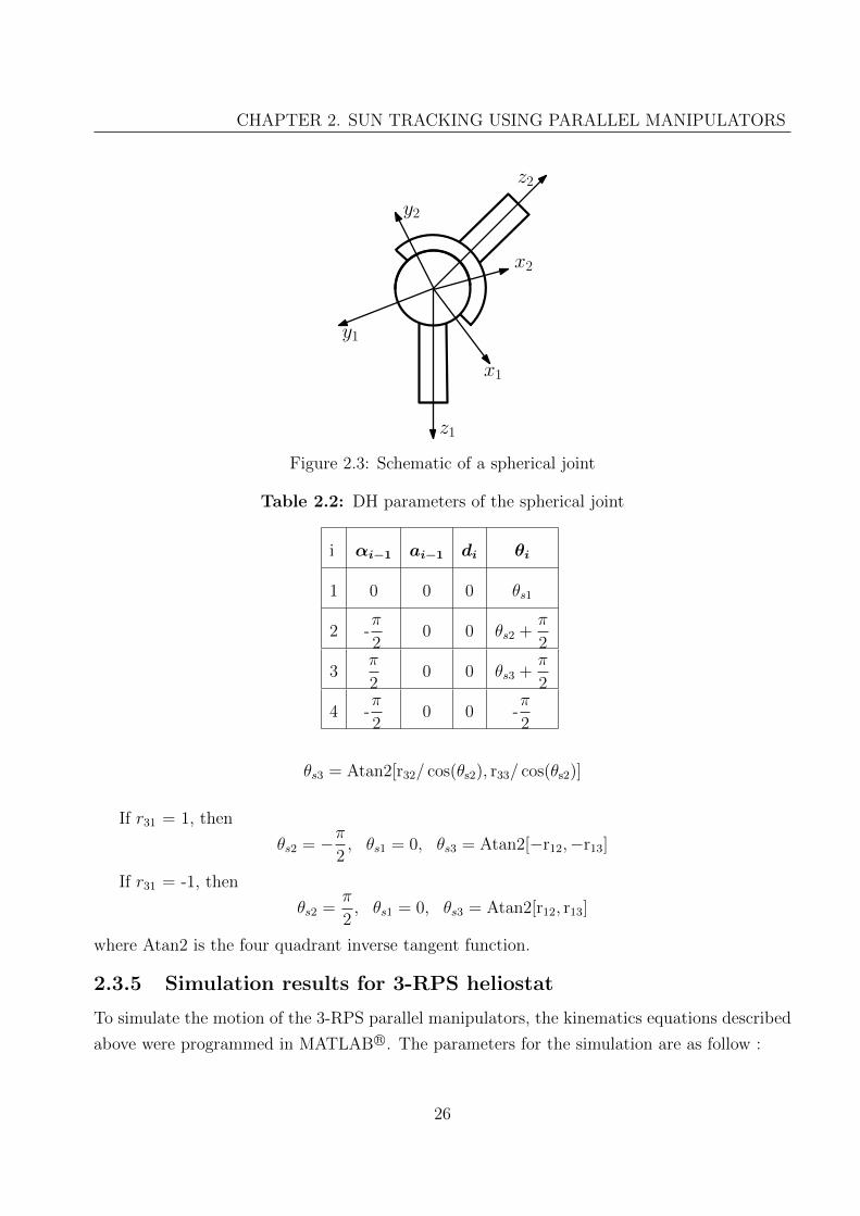
CHAPTER 2. SUN TRACKING USING PARALLEL MANIPULATORS
z1
x1
y1
z2
x2
y2
Figure 2.3: Schematic of a spherical joint
Table 2.2: DH parameters of the spherical joint
i αi−1 ai−1 di θi
1 0 0 0 θs1
2 -π
20 0 θs2 +
π
2
3π
20 0 θs3 +
π
2
4 -π
20 0 -
π
2
θs3 = Atan2[r32/ cos(θs2), r33/ cos(θs2)]
If r31 = 1, then
θs2 = −π2, θs1 = 0, θs3 = Atan2[−r12,−r13]
If r31 = -1, then
θs2 =π
2, θs1 = 0, θs3 = Atan2[r12, r13]
where Atan2 is the four quadrant inverse tangent function.
2.3.5 Simulation results for 3-RPS heliostat
To simulate the motion of the 3-RPS parallel manipulators, the kinematics equations described
above were programmed in MATLAB R©. The parameters for the simulation are as follow :
26
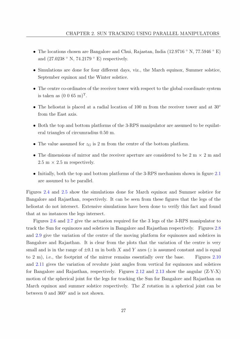
CHAPTER 2. SUN TRACKING USING PARALLEL MANIPULATORS
• The locations chosen are Bangalore and Chui, Rajastan, India (12.9716 ◦ N, 77.5946 ◦ E)
and (27.0238 ◦ N, 74.2179 ◦ E) respectively.
• Simulations are done for four different days, viz., the March equinox, Summer solstice,
September equinox and the Winter solstice.
• The centre co-ordinates of the receiver tower with respect to the global coordinate system
is taken as (0 0 65 m)T.
• The heliostat is placed at a radial location of 100 m from the receiver tower and at 30◦
from the East axis.
• Both the top and bottom platforms of the 3-RPS manipulator are assumed to be equilat-
eral triangles of circumradius 0.50 m.
• The value assumed for zG is 2 m from the centre of the bottom platform.
• The dimensions of mirror and the receiver aperture are considered to be 2 m × 2 m and
2.5 m × 2.5 m respectively.
• Initially, both the top and bottom platforms of the 3-RPS mechanism shown in figure 2.1
are assumed to be parallel.
Figures 2.4 and 2.5 show the simulations done for March equinox and Summer solstice for
Bangalore and Rajasthan, respectively. It can be seen from these figures that the legs of the
heliostat do not intersect. Extensive simulations have been done to verify this fact and found
that at no instances the legs intersect.
Figures 2.6 and 2.7 give the actuation required for the 3 legs of the 3-RPS manipulator to
track the Sun for equinoxes and solstices in Bangalore and Rajasthan respectively. Figures 2.8
and 2.9 give the variation of the centre of the moving platform for equinoxes and solstices in
Bangalore and Rajasthan. It is clear from the plots that the variation of the centre is very
small and is in the range of ±0.1 m in both X and Y axes (z is assumed constant and is equal
to 2 m), i.e., the footprint of the mirror remains essentially over the base. Figures 2.10
and 2.11 gives the variation of revolute joint angles from vertical for equinoxes and solstices
for Bangalore and Rajasthan, respectively. Figures 2.12 and 2.13 show the angular (Z-Y-X)
motion of the spherical joint for the legs for tracking the Sun for Bangalore and Rajasthan on
March equinox and summer solstice respectively. The Z rotation in a spherical joint can be
between 0 and 360◦ and is not shown.
27

CHAPTER 2. SUN TRACKING USING PARALLEL MANIPULATORS
51
Y,No
rth050
1
X, East
86
Z,Ze
nith 2
87 49
3
Normal
Incident ray
Reflected ray
(a) 9 am
51
Y,No
rth050
1
X, East
86
Z,Ze
nith 2
87 49
3
(b) 12 noon
51
Y,No
rth050
1
X, East
86
Z,Ze
nith 2
87 49
3
(c) 2 pm
51
Y,North
500
1
X, East
Z,Ze
nith
86
2
4987
3
(d) 5 pm
Figure 2.4: Simulation of 3-RPS heliostat for March equinox for Bangalore
51
Y,No
rth050
1
X, East
86
Z,Ze
nith 2
87 49
3
Normal
Incident ray
Reflected ray
(a) 9 am
51
Y,No
rth050
1
X, East
86
Z,Ze
nith 2
87 49
3
(b) 12 noon
51
Y,No
rth050
1
X, East
86
Z,Ze
nith 2
87 49
3
(c) 2 pm
51
Y,North
500
X, East
86
1
4987
Z,Ze
nith 2
3
(d) 5 pm
Figure 2.5: Simulation of 3-RPS heliostat for Summer solstice for Rajasthan
28

CHAPTER 2. SUN TRACKING USING PARALLEL MANIPULATORS
6 8 10 12 14 16 18
Time, hrs
1600
1800
2000
2200
2400
2600
leglen
gth,
mm
leg1
leg2
leg3
(a) March equinox
6 8 10 12 14 16 18
Time, hrs
1600
1800
2000
2200
2400
2600
leglen
gth,
mm
leg1
leg2
leg3
(b) Summer solstice
6 8 10 12 14 16 18
Time, hrs
1600
1800
2000
2200
2400
2600
leglen
gth,
mm
leg1
leg2
leg3
(c) September equinox
6 8 10 12 14 16 18
Time, hrs
1600
1800
2000
2200
2400
2600
leglen
gth,
mm
leg1
leg2
leg3
(d) Winter solstice
Figure 2.6: Actuations required for the 3-RPS heliostat in Bangalore
6 8 10 12 14 16 18
Time, hrs
1600
1800
2000
2200
2400
2600
leglen
gth,
mm
leg1
leg2
leg3
(a) March equinox
6 8 10 12 14 16 18
Time, hrs
1600
1800
2000
2200
2400
2600
leglen
gth,
mm
leg1
leg2
leg3
(b) Summer solstice
6 8 10 12 14 16 18
Time, hrs
1600
1800
2000
2200
2400
2600
leglen
gth,
mm
leg1
leg2
leg3
(c) September equinox
6 8 10 12 14 16 18
Time, hrs
1600
1800
2000
2200
2400
2600
leglen
gth,
mm
leg1
leg2
leg3
(d) Winter solstice
Figure 2.7: Actuations required for the 3-RPS heliostat in Rajasthan
29
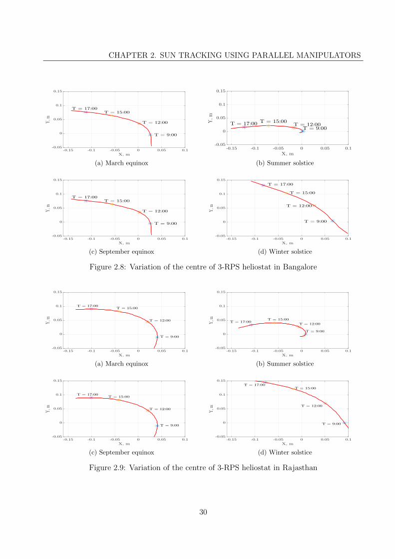
CHAPTER 2. SUN TRACKING USING PARALLEL MANIPULATORS
-0.15 -0.1 -0.05 0 0.05 0.1
X, m
-0.05
0
0.05
0.1
0.15
Y,m
T = 9:00
T = 12:00
T = 15:00T = 17:00
(a) March equinox
-0.15 -0.1 -0.05 0 0.05 0.1
X, m
-0.05
0
0.05
0.1
0.15
Y,m
T = 9:00T = 12:00
T = 15:00T = 17:00
(b) Summer solstice
-0.15 -0.1 -0.05 0 0.05 0.1
X, m
-0.05
0
0.05
0.1
0.15
Y,m
T = 9:00
T = 12:00
T = 15:00T = 17:00
(c) September equinox
-0.15 -0.1 -0.05 0 0.05 0.1
X, m
-0.05
0
0.05
0.1
0.15
Y,m
T = 9:00
T = 12:00
T = 15:00
T = 17:00
(d) Winter solstice
Figure 2.8: Variation of the centre of 3-RPS heliostat in Bangalore
-0.15 -0.1 -0.05 0 0.05 0.1
X, m
-0.05
0
0.05
0.1
0.15
Y,m
T = 9:00
T = 12:00
T = 15:00T = 17:00
(a) March equinox
-0.15 -0.1 -0.05 0 0.05 0.1
X, m
-0.05
0
0.05
0.1
0.15
Y,m
T = 9:00
T = 12:00
T = 15:00T = 17:00
(b) Summer solstice
-0.15 -0.1 -0.05 0 0.05 0.1
X, m
-0.05
0
0.05
0.1
0.15
Y,m
T = 9:00
T = 12:00
T = 15:00T = 17:00
(c) September equinox
-0.15 -0.1 -0.05 0 0.05 0.1
X, m
-0.05
0
0.05
0.1
0.15
Y,m
T = 9:00
T = 12:00
T = 15:00T = 17:00
(d) Winter solstice
Figure 2.9: Variation of the centre of 3-RPS heliostat in Rajasthan
30
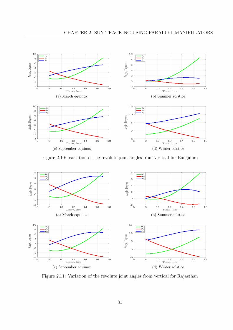
CHAPTER 2. SUN TRACKING USING PARALLEL MANIPULATORS
6 8 10 12 14 16 18
Time, hrs
-4
-2
0
2
4
6
8
10
Ang
le,Degrees
θ1
θ2
θ3
(a) March equinox
6 8 10 12 14 16 18
Time, hrs
-2
0
2
4
6
8
10
Ang
le,Degrees
θ1
θ2
θ3
(b) Summer solstice
6 8 10 12 14 16 18
Time, hrs
-4
-2
0
2
4
6
8
10
Ang
le,Degrees
θ1
θ2
θ3
(c) September equinox
6 8 10 12 14 16 18
Time, hrs
-5
0
5
10
15
Ang
le,Degrees
θ1
θ2
θ3
(d) Winter solstice
Figure 2.10: Variation of the revolute joint angles from vertical for Bangalore
6 8 10 12 14 16 18
Time, hrs
-4
-2
0
2
4
6
8
Ang
le,Degrees
θ1
θ2
θ3
(a) March equinox
6 8 10 12 14 16 18
Time, hrs
-2
0
2
4
6
8
Ang
le,Degrees
θ1
θ2
θ3
(b) Summer solstice
6 8 10 12 14 16 18
Time, hrs
-4
-2
0
2
4
6
8
10
Ang
le,Degrees
θ1
θ2
θ3
(c) September equinox
6 8 10 12 14 16 18
Time, hrs
-5
0
5
10
15
Ang
le,Degrees
θ1
θ2
θ3
(d) Winter solstice
Figure 2.11: Variation of the revolute joint angles from vertical for Rajasthan
31

CHAPTER 2. SUN TRACKING USING PARALLEL MANIPULATORS
6 8 10 12 14 16 18
Time, hrs
-80
-60
-40
-20
0
20
Angle
,Degrees
Rot abt Y
Rot abt X
(a) Leg1
6 8 10 12 14 16 18
Time, hrs
-60
-50
-40
-30
-20
-10
0
10
Angle
,Degrees
Rot abt Y
Rot abt X
(b) Leg2
6 8 10 12 14 16 18
Time, hrs
-80
-60
-40
-20
0
20
Angle
,Degrees
Rot abt Y
Rot abt X
(c) Leg3
Figure 2.12: Variation of the spherical joint angles for Bangalore on March equinox
6 8 10 12 14 16 18
Time, hrs
-80
-60
-40
-20
0
20
Angle
,Degrees
Rot abt Y
Rot abt X
(a) Leg1
6 8 10 12 14 16 18
Time, hrs
-60
-50
-40
-30
-20
-10
0
10
Angle
,Degrees
Rot abt Y
Rot abt X
(b) Leg2
6 8 10 12 14 16 18
Time, hrs
-60
-50
-40
-30
-20
-10
0
10
Angle
,Degrees
Rot abt Y
Rot abt X
(c) Leg3
Figure 2.13: Variation of the spherical joint angles for Rajasthan on summer solstice
One can also obtain the shape of the image on the receiver. To obtain this, we assume
that the ray hitting the centre of the mirror will be reflected towards the centre of the receiver
aperture at every instant of time. Since the mirror is assumed to be perfectly flat and the Sun
32

CHAPTER 2. SUN TRACKING USING PARALLEL MANIPULATORS
is considered to be a point source, the parallel rays hitting the four corners of the mirror will be
reflected to the receiver aperture parallel to the central ray. The points where the reflected rays
from the mirror corner hit the receiver aperture are joined together to form the image polygon.
This is calculated for every one minute interval from 8 a.m. to 5 p.m. In some literatures, this
image area is often mentioned as spot size and the area going out of receiver aperture is called
spillage loss. For the 3-RPS parallel manipulator for the chosen parameters of rb and rp both
equal to 500 mm, the image formed on the receiver plane is shown in figure 2.14 at four instants
of time. This type of analysis helps in quantifying the spillage loss when a 3-RPS heliostat is
used for Sun tracking in CR systems.
-10
X, East
62
64
-1
Z,Zenith 66
68
0
Y, North11
Receiver
3RPS
(a) 9 am
-10
X, East
62
64
-1
Z,Zenith 66
68
0
Y, North11
Receiver
3RPS
(b) 12 noon
-10
X, East
62
64
-1
Z,Zenith 66
68
0
Y, North11
Receiver
3RPS
(c) 2 pm
-10
X, East
62
64
-1
Z,Zenith 66
68
0
Y, North11
Receiver
3RPS
(d) 5 pm
Figure 2.14: The image on the receiver aperture at various time instants for March equinox forBangalore
From simulations done, it is clear that the 3-RPS heliostat does not attain any singular
configurations. The variation of the centre of the top platform, the revolute, prismatic and
the spherical joints are within attainable limits of commercially available products. Thus the
3-RPS parallel manipulator is a promising candidate for prototyping. Further, we look at the
33
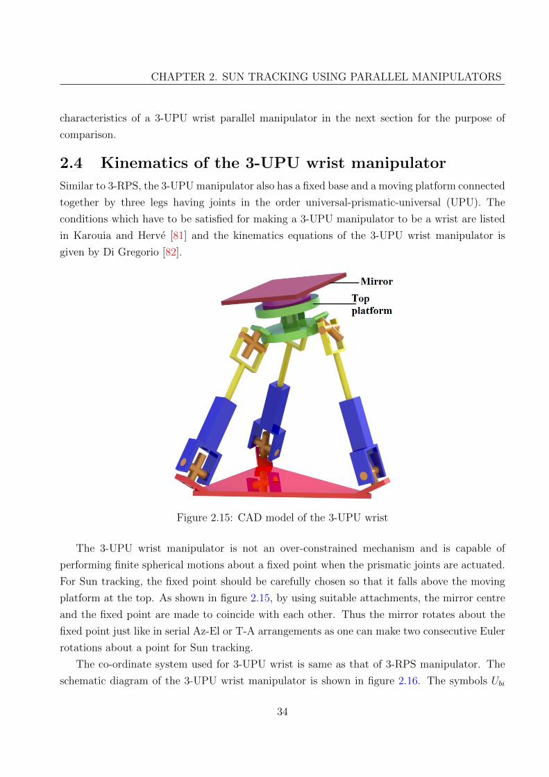
CHAPTER 2. SUN TRACKING USING PARALLEL MANIPULATORS
characteristics of a 3-UPU wrist parallel manipulator in the next section for the purpose of
comparison.
2.4 Kinematics of the 3-UPU wrist manipulator
Similar to 3-RPS, the 3-UPU manipulator also has a fixed base and a moving platform connected
together by three legs having joints in the order universal-prismatic-universal (UPU). The
conditions which have to be satisfied for making a 3-UPU manipulator to be a wrist are listed
in Karouia and Herve [81] and the kinematics equations of the 3-UPU wrist manipulator is
given by Di Gregorio [82].
Figure 2.15: CAD model of the 3-UPU wrist
The 3-UPU wrist manipulator is not an over-constrained mechanism and is capable of
performing finite spherical motions about a fixed point when the prismatic joints are actuated.
For Sun tracking, the fixed point should be carefully chosen so that it falls above the moving
platform at the top. As shown in figure 2.15, by using suitable attachments, the mirror centre
and the fixed point are made to coincide with each other. Thus the mirror rotates about the
fixed point just like in serial Az-El or T-A arrangements as one can make two consecutive Euler
rotations about a point for Sun tracking.
The co-ordinate system used for 3-UPU wrist is same as that of 3-RPS manipulator. The
schematic diagram of the 3-UPU wrist manipulator is shown in figure 2.16. The symbols Ubi
34

CHAPTER 2. SUN TRACKING USING PARALLEL MANIPULATORS
and Uti (i = 1, 2, 3) denote the universal joints at the base and top, respectively. Let the mirror
centre or the fixed point of the 3-UPU wrist be at M. As in the 3-RPS case, the triangles
formed by Ubi and Uti are equilateral triangles whose circum-radius is rb and rp, respectively.
The degrees of freedom of the manipulator as obtained by using equation (2.1) is 3. The
calculations required to find the transformation matrix for Sun tracking in the Az-El or the
T-A mode can be obtained and is described in the next section.
2.4.1 Rotation matrix for Az-El case
X ( East )
Y ( North )
Z ( Zenith )
l1l2
xb
O
ψ
Ub1
Ub2
Ub3
yb
l3
Ut1
Ut2
Ut3
O1
xm
ym
G
zm
RSλ
Receiver
Sun
γzb
Figure 2.16: Schematic of the 3-UPU
In the home position (early morning when the tracking starts), the mirror coordinate system
(xm − ym − zm) is kept parallel to the global coordinate system. Then for an Az-El heliostat,
the two Euler rotations required to track Sun and reflect the rays to the receiver are
1. Rotation about Z by an angle θAz as given by equation (1.5).
2. Rotation about ym by an angle (π2− θEl) as given by equation (1.6)
35

CHAPTER 2. SUN TRACKING USING PARALLEL MANIPULATORS
Hence, the rotation matrix becomes
RAz−El =
cos θAz sin θEl − sin θAz cos θAz cos θEl
sin θAz sin θEl cos θAz sin θAz cos θEl
− cos θEl 0 sin θEl
(2.16)
In such a rotation, the ym axis of the mirror coordinate system would still lie on a plane parallel
to the XY plane and it is verified by noting that the (3,2) element of the rotation matrix, RAz−El,
is zero. The third column of the rotation matrix are the direction cosines of the normal−−→GN
which is already known from equation (1.4). The other two columns of the rotation matrix are
found out by carrying out suitable inverse trigonometric calculations.
The above same rotation matrix can also be found out using numerical approach. A general
rotation matrix contains (n1, n2, n3)T , (o1, o2, o3)
T and (a1, a2, a3)T as its first, second and third
column (see equation (2.2), respectively. For Az-El rotation, we have o3 = 0 and (a1 a2 a3)T is
obtained from equation (1.4). Thus we have five equations from the orthogonality of the rotation
matrix and five unknowns, viz., n1, n2, n3, o1 and o2. Using MATLAB R©’s fsolve routine, these
five equations are solved to get the values of n1, n2, n3, o1 and o2. The actuations required is
dependent on the initial conditions of the fsolve routine and have to be chosen carefully.
2.4.2 Rotation matrix for Target-Aligned heliostat
The initial rotation matrix required is given by equation (1.7). Then the heliostat spins about−→GR by θsp given by equation (1.8) and rotates about ym by θel given by equation (1.9). The
spinning and elevation rotation matrix is given by
R34 =
cos θsp cos θel − sin θsp cos θsp sin θel
sin θsp cos θel cos θsp sin θsp sin θel
− sin θel 0 cos θel
36

CHAPTER 2. SUN TRACKING USING PARALLEL MANIPULATORS
Thus the final rotation matrix for the T-A heliostat is given by RT−A = R12R34 =
cψcλcθspcθel − sψsθspcθel + cψsλsθel −cψcλsθsp − sψcθsp cψcλcθspsθel − sψsθspsθel − cψsλcθel
sψcλcθspcθel + cψsθspcθel + sψsλsθel −sψcλsθsp + cψcθsp sψcλcθspsθel + cψsθspsθel − sψsλcθel
sλcθspcθel − cλsθel −sλsθsp sλcθspsθel + cλcθel
where cz, sz represents the cosine and sine of the respective angles given by z. Like in Az-El
heliostat, the normal−−→GN and hence the third column of RT−A is known. The angles ψ and λ
are known from the prior knowledge of location of heliostat in the field and centre co-ordinates
of the receiver with respect to the global coordinate system. Thus the first and second columns
of the rotation matrix RT−A can be computed.
2.4.3 Actuations required for 3-UPU wrist
As mentioned earlier, the top-platform and the mirror are connected together using an at-
tachment such that the orientation of both are the same with respect to the base. The only
difference being the centre of the mirror remains at the fixed point even while executing finite
spherical rotations whereas it is not the same for the top platform. Initially, both the top and
bottom platforms are assumed to be parallel. Then the rotation which takes the mirror to the
base is found out as mentioned in sections 2.4.1 and 2.4.2. The centre of the top platform will
be at a constant distance from the mirror centre in its normal direction downwards. Using this
information, the centre of the top platform is found out and hence the actuation required for
the legs of 3-UPU wrist can be found out as follows:
Similar to 3-RPS, for the 3-UPU manipulator, the co-ordinates of the Ubi joints with
respect to {B} are given by−−−→O1Ub1 = (rb, 0, 0)T ,
−−−→O1Ub2 = (−1
2rb,√32rb, 0)T and
−−−→O1Ub3 =
(−12rb,−
√32rb, 0)T and the co-ordinates of the Uti joints with respect to {xm, ym, zm} are given
by−−→GUt1 = (rp, 0, 0)T ,
−−→GUt2 = (−1
2rp,√32rp, 0)T and
−−→GUt3 = (−1
2rp,−
√32rp, 0)T . The position
vector of the top U joints with respect to the base co-ordinate system {B} is given as−−−→O1Uti
1
=[T]−−→GUti
1
37
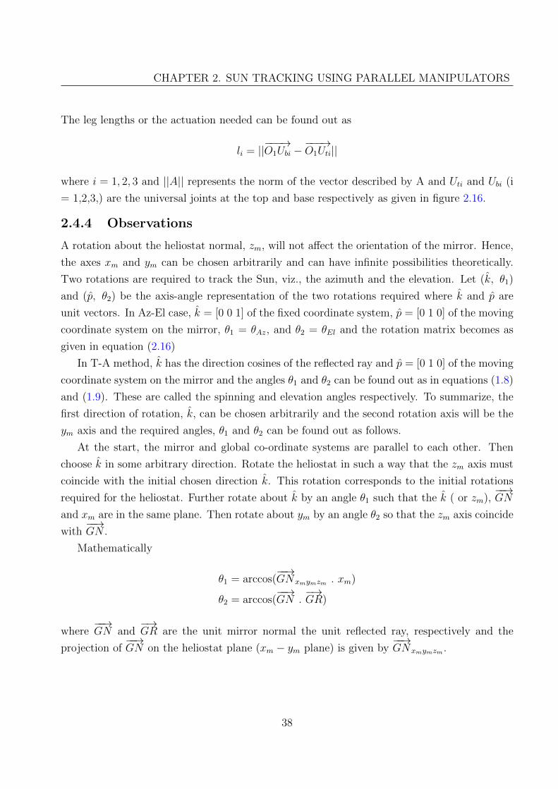
CHAPTER 2. SUN TRACKING USING PARALLEL MANIPULATORS
The leg lengths or the actuation needed can be found out as
li = ||−−−→O1Ubi −−−−→O1Uti||
where i = 1, 2, 3 and ||A|| represents the norm of the vector described by A and Uti and Ubi (i
= 1,2,3,) are the universal joints at the top and base respectively as given in figure 2.16.
2.4.4 Observations
A rotation about the heliostat normal, zm, will not affect the orientation of the mirror. Hence,
the axes xm and ym can be chosen arbitrarily and can have infinite possibilities theoretically.
Two rotations are required to track the Sun, viz., the azimuth and the elevation. Let (k, θ1)
and (p, θ2) be the axis-angle representation of the two rotations required where k and p are
unit vectors. In Az-El case, k = [0 0 1] of the fixed coordinate system, p = [0 1 0] of the moving
coordinate system on the mirror, θ1 = θAz, and θ2 = θEl and the rotation matrix becomes as
given in equation (2.16)
In T-A method, k has the direction cosines of the reflected ray and p = [0 1 0] of the moving
coordinate system on the mirror and the angles θ1 and θ2 can be found out as in equations (1.8)
and (1.9). These are called the spinning and elevation angles respectively. To summarize, the
first direction of rotation, k, can be chosen arbitrarily and the second rotation axis will be the
ym axis and the required angles, θ1 and θ2 can be found out as follows.
At the start, the mirror and global co-ordinate systems are parallel to each other. Then
choose k in some arbitrary direction. Rotate the heliostat in such a way that the zm axis must
coincide with the initial chosen direction k. This rotation corresponds to the initial rotations
required for the heliostat. Further rotate about k by an angle θ1 such that the k ( or zm),−−→GN
and xm are in the same plane. Then rotate about ym by an angle θ2 so that the zm axis coincide
with−−→GN .
Mathematically
θ1 = arccos(−−→GNxmymzm . xm)
θ2 = arccos(−−→GN .
−→GR)
where−−→GN and
−→GR are the unit mirror normal the unit reflected ray, respectively and the
projection of−−→GN on the heliostat plane (xm − ym plane) is given by
−−→GNxmymzm .
38

CHAPTER 2. SUN TRACKING USING PARALLEL MANIPULATORS
2.4.5 Simulation results for 3-UPU wrist
The parameters used for 3-UPU simulation are same as that of 3-RPS. The fixed point of
the 3-UPU wrist is at a height of 2 m from the bottom platform. The plot of the image
on the receiver plane for a 3-UPU wrist working in Az-EL and T-A methods are shown in
figure 2.17 Figure 2.18 shows the simulation results for various time instants for March equinox
-10
X, East
62
64
-1
Z,Zenith 66
68
0
Y, North11
Receiver
AzEl
TA
(a) 9 am
-10
X, East
62
64
-1
Z,Zenith 66
68
0
Y, North11
Receiver
AzEl
TA
(b) 12 noon
-10
X, East
62
64
-1
Z,Zenith 66
68
0
Y, North11
Receiver
AzEl
TA
(c) 2 pm
-10
X, East
62
64
-1
Z,Zenith 66
68
0
Y, North11
Receiver
AzEl
TA
(d) 5 pm
Figure 2.17: The image on the receiver aperture at various time instants for March equinox forBangalore
in Bangalore if the 3-UPU wrist is to be used in T-A method. It is clearly understood from
figure 2.18d that the legs of the 3-UPU wrist intersect each other during the evening time. In
order to prevent this, the rotation matrix obtained using T-A method can be multiplied by a
rotation about the mirror normal so that the legs of the 3-UPU will not intersect. Figure 2.19
shows the modified simulation results when the T-A rotation matrix is multiplied by another
rotation about mirror normal by 60◦. The actuations required fpr T-A and modified T-A are
39

CHAPTER 2. SUN TRACKING USING PARALLEL MANIPULATORS
0
49
1
2
Z,Ze
nith
3
86Y, North
50
X, East
8751
(a) 9 am
0
49
1
86Y, North
50
X, East
Z,Ze
nith
2
87
3
51
(b) 12 noon
0
49
1
86
Z,Ze
nith
2
Y, North
50
X, East
3
87
51
(c) 2 pm
0
49
1
2
Z,Ze
nith
3
86Y, North
50
X, East
8751
(d) 5 pm
Figure 2.18: Simulation of 3-UPU wrist for T-A mode for March equinox for Bangalore
49
Y,No
rth
50
0
X, East
87.5 87
1
5186.5 86
Z,Ze
nith
2
3
(a) 9 am
49
Y,North50
0
87.5
X, East
1
8786.5 5186
Z,Ze
nith
2
3
(b) 12 noon
49
Y,North50
0
87.5
1
87X, East
86.5
Z,Ze
nith
2
86 51
3
(c) 2 pm
0
49
1
2
87
Z,Ze
nith
X, East Y,No
rth
3
50
8651
(d) 5 pm
Figure 2.19: Simulation of 3-UPU wrist for modified T-A mode for March equinox for Bangalore
40
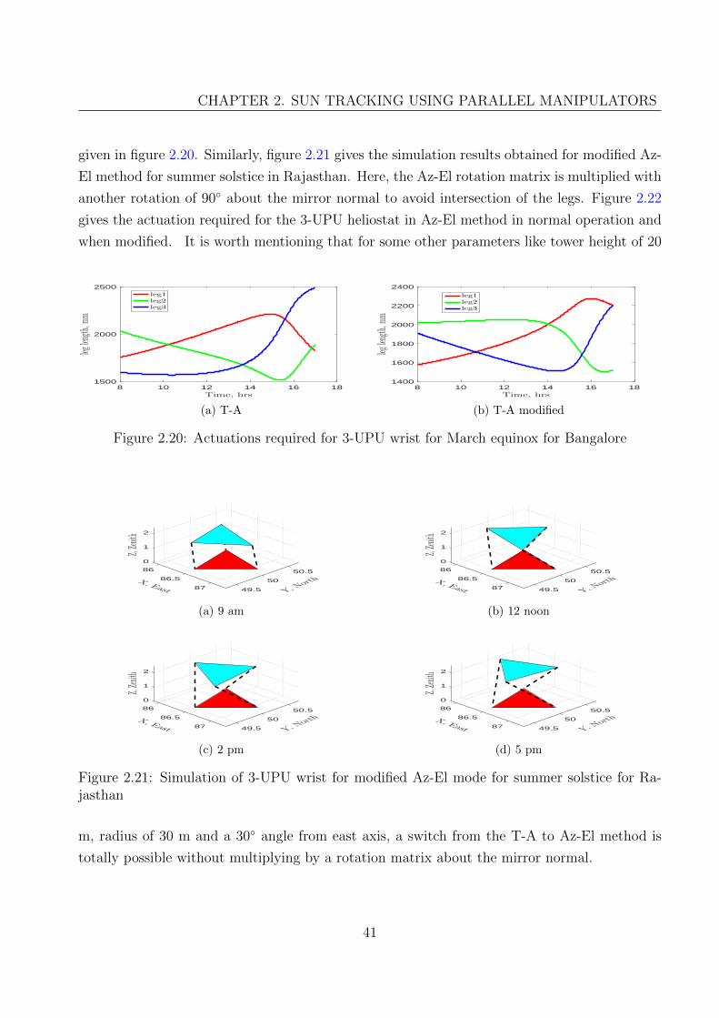
CHAPTER 2. SUN TRACKING USING PARALLEL MANIPULATORS
given in figure 2.20. Similarly, figure 2.21 gives the simulation results obtained for modified Az-
El method for summer solstice in Rajasthan. Here, the Az-El rotation matrix is multiplied with
another rotation of 90◦ about the mirror normal to avoid intersection of the legs. Figure 2.22
gives the actuation required for the 3-UPU heliostat in Az-El method in normal operation and
when modified. It is worth mentioning that for some other parameters like tower height of 20
8 10 12 14 16 18
Time, hrs
1500
2000
2500
leglen
gth,
mm
leg1
leg2
leg3
(a) T-A
8 10 12 14 16 18
Time, hrs
1400
1600
1800
2000
2200
2400
leglen
gth,
mm
leg1
leg2
leg3
(b) T-A modified
Figure 2.20: Actuations required for 3-UPU wrist for March equinox for Bangalore
0
8650.5
86.5X, East Y,No
rth
1
50
Z,Ze
nith
8749.5
2
(a) 9 am
0
8650.5
86.5X, East Y,No
rth
1
50
Z,Ze
nith
8749.5
2
(b) 12 noon
0
8650.5
86.5X, East Y,No
rth
1
50
Z,Ze
nith
8749.5
2
(c) 2 pm
0
8650.5
86.5X, East Y,No
rth
1
50
Z,Ze
nith
8749.5
2
(d) 5 pm
Figure 2.21: Simulation of 3-UPU wrist for modified Az-El mode for summer solstice for Ra-jasthan
m, radius of 30 m and a 30◦ angle from east axis, a switch from the T-A to Az-El method is
totally possible without multiplying by a rotation matrix about the mirror normal.
41
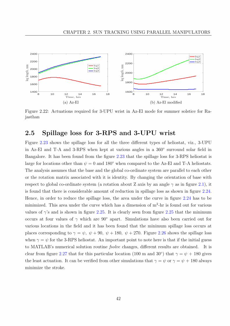
CHAPTER 2. SUN TRACKING USING PARALLEL MANIPULATORS
8 10 12 14 16 18
Time, hrs
1400
1600
1800
2000
2200
2400
legleng
th,m
m leg1
leg2
leg3
(a) Az-El
8 10 12 14 16 18
Time, hrs
1600
1800
2000
2200
2400
legleng
th,m
m
leg1
leg2
leg3
(b) Az-El modified
Figure 2.22: Actuations required for 3-UPU wrist in Az-El mode for summer solstice for Ra-jasthan
2.5 Spillage loss for 3-RPS and 3-UPU wrist
Figure 2.23 shows the spillage loss for all the three different types of heliostat, viz., 3-UPU
in Az-El and T-A and 3-RPS when kept at various angles in a 360◦ surround solar field in
Bangalore. It has been found from the figure 2.23 that the spillage loss for 3-RPS heliostat is
large for locations other than ψ = 0 and 180◦ when compared to the Az-El and T-A heliostats.
The analysis assumes that the base and the global co-ordinate system are parallel to each other
or the rotation matrix associated with it is identity. By changing the orientation of base with
respect to global co-ordinate system (a rotation about Z axis by an angle γ as in figure 2.1), it
is found that there is considerable amount of reduction in spillage loss as shown in figure 2.24.
Hence, in order to reduce the spillage loss, the area under the curve in figure 2.24 has to be
minimized. This area under the curve which has a dimension of m2-hr is found out for various
values of γ’s and is shown in figure 2.25. It is clearly seen from figure 2.25 that the minimum
occurs at four values of γ which are 90◦ apart. Simulations have also been carried out for
various locations in the field and it has been found that the minimum spillage loss occurs at
places corresponding to γ = ψ, ψ + 90, ψ + 180, ψ + 270. Figure 2.26 shows the spillage loss
when γ = ψ for the 3-RPS heliostat. An important point to note here is that if the initial guess
to MATLAB’s numerical solution routine fsolve changes, different results are obtained. It is
clear from figure 2.27 that for this particular location (100 m and 30◦) that γ = ψ + 180 gives
the least actuation. It can be verified from other simulations that γ = ψ or γ = ψ + 180 always
minimize the stroke.
42
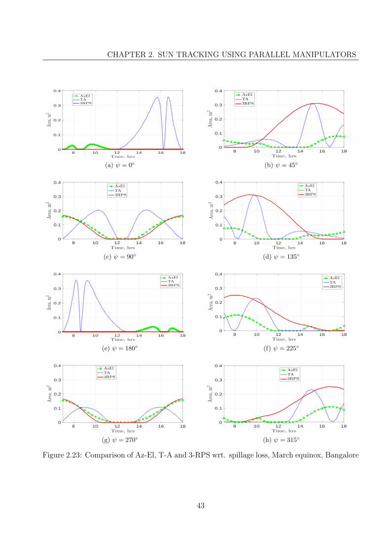
CHAPTER 2. SUN TRACKING USING PARALLEL MANIPULATORS
8 10 12 14 16 18
Time, hrs
0
0.1
0.2
0.3
0.4
Area,
m2
AzEl
TA
3RPS
(a) ψ = 0◦
8 10 12 14 16 18
Time, hrs
0
0.1
0.2
0.3
0.4
Area,
m2
AzEl
TA
3RPS
(b) ψ = 45◦
8 10 12 14 16 18
Time, hrs
0
0.1
0.2
0.3
0.4
Area,
m2
AzEl
TA
3RPS
(c) ψ = 90◦
8 10 12 14 16 18
Time, hrs
0
0.1
0.2
0.3
0.4
Area,
m2
AzEl
TA
3RPS
(d) ψ = 135◦
8 10 12 14 16 18
Time, hrs
0
0.1
0.2
0.3
0.4
Area,
m2
AzEl
TA
3RPS
(e) ψ = 180◦
8 10 12 14 16 18
Time, hrs
0
0.1
0.2
0.3
0.4
Area,
m2
AzEl
TA
3RPS
(f) ψ = 225◦
8 10 12 14 16 18
Time, hrs
0
0.1
0.2
0.3
0.4
Area,
m2
AzEl
TA
3RPS
(g) ψ = 270◦
8 10 12 14 16 18
Time, hrs
0
0.1
0.2
0.3
0.4
Area,
m2
AzEl
TA
3RPS
(h) ψ = 315◦
Figure 2.23: Comparison of Az-El, T-A and 3-RPS wrt. spillage loss, March equinox, Bangalore
43

CHAPTER 2. SUN TRACKING USING PARALLEL MANIPULATORS
8 10 12 14 16 18
Time, hrs
0
0.05
0.1
0.15
0.2
0.25
0.3
Area,
m2
γ = 100
γ = 200
γ = 300
Figure 2.24: Variation of spillage loss with γ for 3-RPS for March equinox, Bangalore
2.6 Conclusions and challenges ahead
In this chapter, we have proposed two parallel manipulators which can be used for tracking the
Sun. Both these have three degrees of freedom and thus require three actuators. The kinematics
of the 3-RPS and the 3-UPU parallel manipulator, for Sun tracking, are developed. From the
solution of the kinematics equations, the change in the lengths of the prismatic joint required to
track the Sun are determined. Simulation results show that the legs of the 3-UPU wrist might
intersect whereas this does not happen for 3-RPS. For 3-UPU wrist, extensive simulations are
needed for locations other than Bangalore and Rajasthan to know by what amount the top-
platform has to be rotated to prevent intersection of legs. For 3-RPS heliostat, the spillage loss
and actuation is minimized by keeping the orientation of base platform γ = ψ or γ = ψ + 180◦.
44
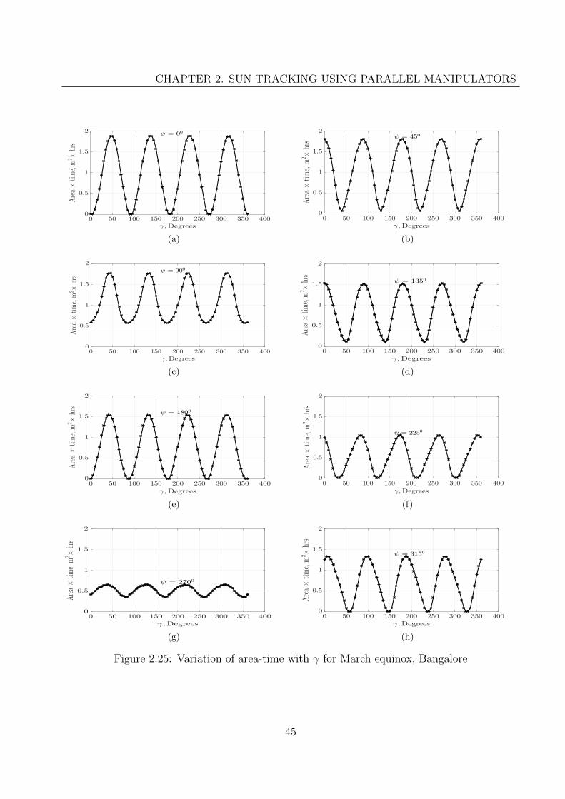
CHAPTER 2. SUN TRACKING USING PARALLEL MANIPULATORS
0 50 100 150 200 250 300 350 400
γ,Degrees
0
0.5
1
1.5
2
Area×
time,
m2 ×
hrs
ψ = 00
(a)
0 50 100 150 200 250 300 350 400
γ,Degrees
0
0.5
1
1.5
2
Area×
time,
m2 ×
hrs
ψ = 450
(b)
0 50 100 150 200 250 300 350 400
γ,Degrees
0
0.5
1
1.5
2
Area×
time,
m2 ×
hrs
ψ = 900
(c)
0 50 100 150 200 250 300 350 400
γ,Degrees
0
0.5
1
1.5
2
Area×
time,
m2 ×
hrs
ψ = 1350
(d)
0 50 100 150 200 250 300 350 400
γ,Degrees
0
0.5
1
1.5
2
Area×
time,
m2 ×
hrs
ψ = 1800
(e)
0 50 100 150 200 250 300 350 400
γ,Degrees
0
0.5
1
1.5
2
Area×
time,
m2×
hrs
ψ = 2250
(f)
0 50 100 150 200 250 300 350 400
γ,Degrees
0
0.5
1
1.5
2
Area×
time,
m2 ×
hrs
ψ = 2700
(g)
0 50 100 150 200 250 300 350 400
γ,Degrees
0
0.5
1
1.5
2
Area×
time,
m2 ×
hrs
ψ = 3150
(h)
Figure 2.25: Variation of area-time with γ for March equinox, Bangalore
45
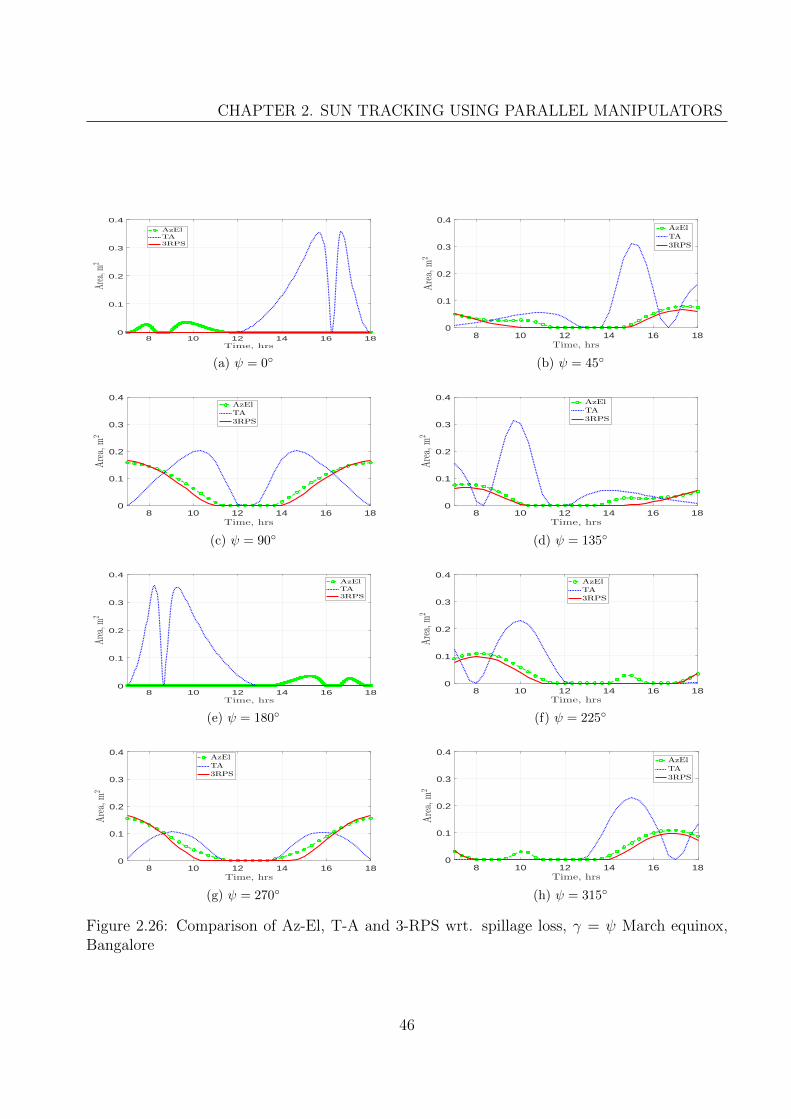
CHAPTER 2. SUN TRACKING USING PARALLEL MANIPULATORS
8 10 12 14 16 18
Time, hrs
0
0.1
0.2
0.3
0.4
Area,
m2
AzEl
TA
3RPS
(a) ψ = 0◦
8 10 12 14 16 18
Time, hrs
0
0.1
0.2
0.3
0.4
Area,
m2
AzEl
TA
3RPS
(b) ψ = 45◦
8 10 12 14 16 18
Time, hrs
0
0.1
0.2
0.3
0.4
Area,
m2
AzEl
TA
3RPS
(c) ψ = 90◦
8 10 12 14 16 18
Time, hrs
0
0.1
0.2
0.3
0.4
Area,
m2
AzEl
TA
3RPS
(d) ψ = 135◦
8 10 12 14 16 18
Time, hrs
0
0.1
0.2
0.3
0.4
Area,
m2
AzEl
TA
3RPS
(e) ψ = 180◦
8 10 12 14 16 18
Time, hrs
0
0.1
0.2
0.3
0.4
Area,
m2
AzEl
TA
3RPS
(f) ψ = 225◦
8 10 12 14 16 18
Time, hrs
0
0.1
0.2
0.3
0.4
Area,
m2
AzEl
TA
3RPS
(g) ψ = 270◦
8 10 12 14 16 18
Time, hrs
0
0.1
0.2
0.3
0.4
Area,
m2
AzEl
TA
3RPS
(h) ψ = 315◦
Figure 2.26: Comparison of Az-El, T-A and 3-RPS wrt. spillage loss, γ = ψ March equinox,Bangalore
46

CHAPTER 2. SUN TRACKING USING PARALLEL MANIPULATORS
l1 l2 l3
-2000
200400
Length,mm
ψ = 300; γ = 300
l1 l2 l3
-400-200
0200400
Length,mm
ψ = 300; γ = 1200
l1 l2 l3
-400
-200
0
200
400
Length,mm
ψ = 300; γ = 2100
l1 l2 l3
-400-200
0200400
Length,mm ψ = 300; γ = 3000
30 120 210 300
γ, Degrees
0
500
1000
Stroke,mm
Figure 2.27: Variation of stroke with γ for March equinox, Bangalore
47

Chapter 3
Structural design of a 3-RPS heliostat
3.1 Introduction
In chapter 2, simulations for the 3-RPS and 3-UPU wrist manipulators for Sun tracking in cen-
tral receiver systems were carried out. It was observed that the 3-UPU wrist requires precision
manufacturing to get a fixed point for using it as a heliostat in CR systems. Additionally, for
certain times, the kinematics resulted in the intersection of the legs. Due to these disadvantages,
the 3-RPS parallel manipulator configuration was chosen for further study with a goal to design
3-RPS based heliostat for central receiver systems. In any heliostat, the design for wind loading
is an important aspect as the heliostat deformation should not lead to loss in pointing accuracy
and during high winds, although the heliostat would not be in use, it should not fail. This
chapter mainly deals with the design of support structure against wind and gravity loading.
As mentioned in previous chapter, in the 3-RPS configuration, the actuators are connected to
the top and bottom platform at three points. This inherently reduces the load acting on each
leg as it is shared by the three legs. Nevertheless some structural support material is required
such that there is enough stiffness to withstand the wind loading and the pointing errors at the
ends are limited to 2 or 3 mrad. Various frame designs were considered for single point support
(Az-El and T-A) and the 3-RPS heliostats. It is shown in this chapter that for large mirrors,
there is significant amount of weight reduction for the 3-RPS support structure compared to
the single point supports in traditional Az-El and T-A mounts for the same required pointing
accuracy. As shown in the previous chapter, a 3-RPS design has several variables such as the
top platform and bottom platform circum-radii and an angle locating the first mount point. In
this chapter, we perform a search based optimization to obtain optimized values of the 3-RPS
design variables. We obtain designs which give the least weight of the support structure for
a pre-defined wind and gravity loading and which results in least stroke in the prismatic join
48
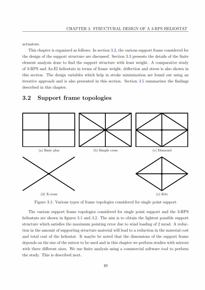
CHAPTER 3. STRUCTURAL DESIGN OF A 3-RPS HELIOSTAT
actuators.
This chapter is organized as follows: In section 3.2, the various support frame considered for
the design of the support structure are discussed. Section 3.3 presents the details of the finite
element analysis done to find the support structure with least weight. A comparative study
of 3-RPS and Az-El heliostats in terms of frame weight, deflection and stress is also shown in
this section. The design variables which help in stroke minimization are found out using an
iterative approach and is also presented in this section. Section 3.5 summarizes the findings
described in this chapter.
3.2 Support frame topologies
(a) Basic plus (b) Simple cross (c) Diamond
(d) X-cross (e) Kite
Figure 3.1: Various types of frame topologies considered for single point support
The various support frame topologies considered for single point support and the 3-RPS
heliostats are shown in figures 3.1 and 3.2. The aim is to obtain the lightest possible support
structure which satisfies the maximum pointing error due to wind loading of 2 mrad. A reduc-
tion in the amount of supporting structure material will lead to a reduction in the material cost
and total cost of the heliostat. It maybe be noted that the dimensions of the support frame
depends on the size of the mirror to be used and in this chapter we perform studies with mirrors
with three different sizes. We use finite analysis using a commercial software tool to perform
the study. This is described next.
49

CHAPTER 3. STRUCTURAL DESIGN OF A 3-RPS HELIOSTAT
rp
(a)
rp
(b)
rp
(c)
Figure 3.2: Various types of frame topologies considered for 3RPS heliostat
3.3 Finite element modeling of mirror and support struc-
ture
The finite element analysis of the mirror and support structure is carried out in ANSYS R©
Workbench [83]. The element types used are SOLID186 and SOLID187 with three degrees-
of-freedom per node. Program controlled automatic meshing is enabled for the analysis. The
mesh size is refined in each iteration until convergence is achieved.
The deformation of the mirror and support structure is found out for its self-weight and
for a survival wind speed, v of 22 m/s and an operational wind speed, v of 10 m/s. It has
to be noted that the wind speeds (both survival and operational) depend upon the geographic
location and may not be the same value for all places. The guidelines for wind load calculation
are given in [84, 85]. The structure is kept vertically and the wind pressure is assumed to be
acting normal to the surface so that the worst case scenario can be simulated. The factor of
safety (FoS) used for the analysis is 2.0. The uniform wind load P on the surface of the mirror
is calculated by using the equation
P =1
2Cdρv
2FoS
where Cd = 1.18 [86] is the drag coefficient and ρ is the density of air assumed to be 1.25
kg/m3 (see figure 3.3). The mirror is assumed to be made of float glass weighing 10 kg/m2
and the material chosen for support structure is plain carbon steel with density, ρ = 7800
kg/m3. The CAD model of the support structure and the mirror is made in SolidWorks R© [87]
by parametric modeling technique which allows one to make changes in the model parameters
such as length, width, height, radius of curves etc. fairly easily. Then the two are mated to
obtain a single object and then ported to ANSYS R© Workbench for finite element analysis.
50

CHAPTER 3. STRUCTURAL DESIGN OF A 3-RPS HELIOSTAT
Figure 3.3: Uniform wind load acting on a 5 m x 5 m mirror
The stresses and deformation due to the wind and self-weight loading are computed by doing
FEA. The parametric modeling technique also helps to identify the lightest possible support
structure which could withstand the 2 mrad maximum deflection criteria. Three mirror sizes,
viz., 2 m×2 m, 3 m×3 m and 5 m×5 m are considered for the study to determine the support
structure with least weight for each of the mirror dimensions. The goal is to obtain the lightest
possible support structure, reduce stroke, satisfy the maximum deformation requirements and
thus reduce material cost of the heliostat.
3.3.1 Search for rp
With reference to the figure 2.1, the connection points at the top platform defined by the length
rp from the centre, G, has got two significant functions. As the distance of the connection points
from the centre increases, the stroke required to get the same orientation also increases. The
other significance is that a large value for rp, tends to increase the deformation of the mirror
at the centre due to wind and gravity loading whereas a small value corresponds to large
deformation at the edges. Of the above two, the most critical criteria is on the deformation
which is to be within a error limit of 2 - 3 mrad. Hence a finite element analysis is carried out
to find out the deflections by varying rp iteratively. For 2 m × 2 m, 3 m × 3 m and 5 m ×5 m mirror, the value of rp thus obtained are 500, 900 and 1800 mm respectively. Table 3.1
51
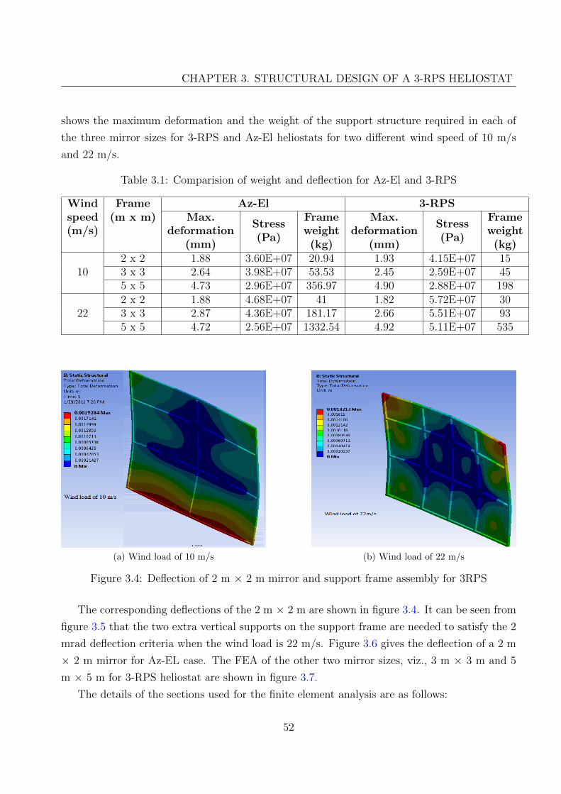
CHAPTER 3. STRUCTURAL DESIGN OF A 3-RPS HELIOSTAT
shows the maximum deformation and the weight of the support structure required in each of
the three mirror sizes for 3-RPS and Az-El heliostats for two different wind speed of 10 m/s
and 22 m/s.
Table 3.1: Comparision of weight and deflection for Az-El and 3-RPS
Windspeed(m/s)
Frame(m x m)
Az-El 3-RPSMax.
deformation(mm)
Stress(Pa)
Frameweight(kg)
Max.deformation
(mm)
Stress(Pa)
Frameweight(kg)
102 x 2 1.88 3.60E+07 20.94 1.93 4.15E+07 153 x 3 2.64 3.98E+07 53.53 2.45 2.59E+07 455 x 5 4.73 2.96E+07 356.97 4.90 2.88E+07 198
222 x 2 1.88 4.68E+07 41 1.82 5.72E+07 303 x 3 2.87 4.36E+07 181.17 2.66 5.51E+07 935 x 5 4.72 2.56E+07 1332.54 4.92 5.11E+07 535
(a) Wind load of 10 m/s (b) Wind load of 22 m/s
Figure 3.4: Deflection of 2 m × 2 m mirror and support frame assembly for 3RPS
The corresponding deflections of the 2 m × 2 m are shown in figure 3.4. It can be seen from
figure 3.5 that the two extra vertical supports on the support frame are needed to satisfy the 2
mrad deflection criteria when the wind load is 22 m/s. Figure 3.6 gives the deflection of a 2 m
× 2 m mirror for Az-EL case. The FEA of the other two mirror sizes, viz., 3 m × 3 m and 5
m × 5 m for 3-RPS heliostat are shown in figure 3.7.
The details of the sections used for the finite element analysis are as follows:
52

CHAPTER 3. STRUCTURAL DESIGN OF A 3-RPS HELIOSTAT
(a) Wind load of 10 m/s (b) Wind load of 22 m/s
Figure 3.5: Support frame of a 2 m × 2 m mirror for 3-RPS
(a) Wind load of 10 m/s (b) Wind load of 22 m/s
Figure 3.6: Deflections of the 2 m × 2 m mirror for Az-El heliostat
1. Wind speed of 22 m/s
• For 2 m × 2 m the results are for square box section of size 30 mm and wall thickness
of 2 mm.
• For 3 m × 3 m the results are for square box section of size 50 mm and wall thickness
of 2 mm.
53
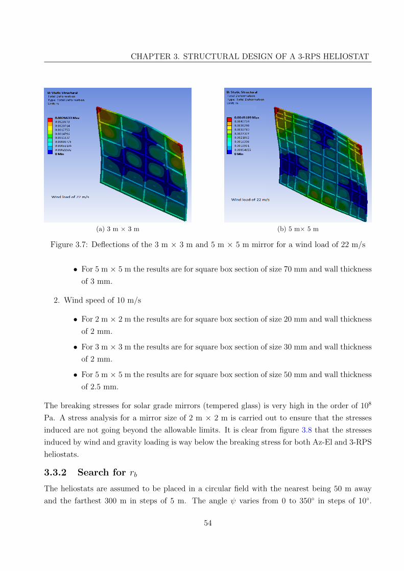
CHAPTER 3. STRUCTURAL DESIGN OF A 3-RPS HELIOSTAT
(a) 3 m × 3 m (b) 5 m× 5 m
Figure 3.7: Deflections of the 3 m × 3 m and 5 m × 5 m mirror for a wind load of 22 m/s
• For 5 m × 5 m the results are for square box section of size 70 mm and wall thickness
of 3 mm.
2. Wind speed of 10 m/s
• For 2 m × 2 m the results are for square box section of size 20 mm and wall thickness
of 2 mm.
• For 3 m × 3 m the results are for square box section of size 30 mm and wall thickness
of 2 mm.
• For 5 m × 5 m the results are for square box section of size 50 mm and wall thickness
of 2.5 mm.
The breaking stresses for solar grade mirrors (tempered glass) is very high in the order of 108
Pa. A stress analysis for a mirror size of 2 m × 2 m is carried out to ensure that the stresses
induced are not going beyond the allowable limits. It is clear from figure 3.8 that the stresses
induced by wind and gravity loading is way below the breaking stress for both Az-El and 3-RPS
heliostats.
3.3.2 Search for rb
The heliostats are assumed to be placed in a circular field with the nearest being 50 m away
and the farthest 300 m in steps of 5 m. The angle ψ varies from 0 to 350◦ in steps of 10◦.
54

CHAPTER 3. STRUCTURAL DESIGN OF A 3-RPS HELIOSTAT
(a) 10 m/s 3-RPS (b) 22 m/s 3-RPS
(c) 10 m/s Az-El (d) 22 m/s Az-El
Figure 3.8: Stresses induced on a 2 m × 2 m
To make the analysis computationally inexpensive, only four days (the solstices and equinoxes)
are considered. Depending upon the direction of incoming Sun rays, the actuation required
are more for the heliostats which are nearest and farthest from the receiver tower compared
to the heliostats in between. Hence the analysis is done only for an array of heliostats at
radii of 50 m and 300 m. Initially, the heliostat is parallel with the ground plane and is
considered to be the zero actuation position. Actuations above and below zero are considered
positive and negative respectively. For any other orientation, the point on the ground where
the perpendicular dropped from the connection point meets, gives the position of rb for least
actuation required. Since the heliostat is required to have several orientations to track the Sun,
rb changes with time. It is also found that for each ψ, the value of rb which minimizes the stroke
55
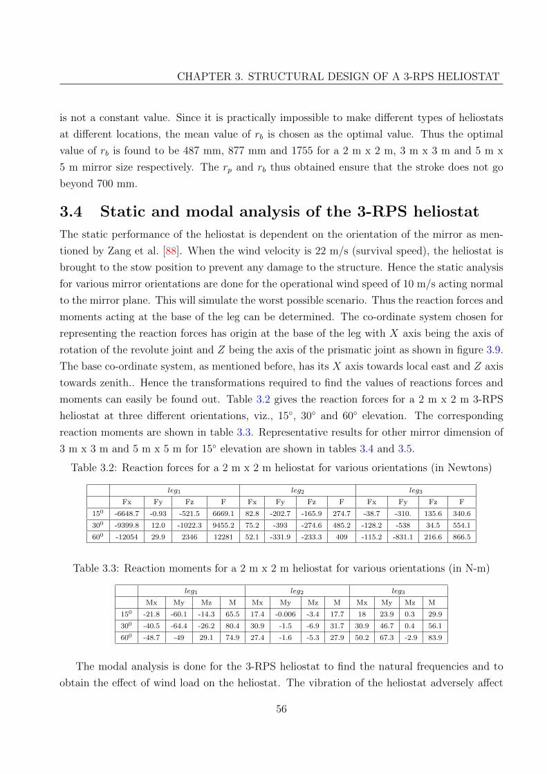
CHAPTER 3. STRUCTURAL DESIGN OF A 3-RPS HELIOSTAT
is not a constant value. Since it is practically impossible to make different types of heliostats
at different locations, the mean value of rb is chosen as the optimal value. Thus the optimal
value of rb is found to be 487 mm, 877 mm and 1755 for a 2 m x 2 m, 3 m x 3 m and 5 m x
5 m mirror size respectively. The rp and rb thus obtained ensure that the stroke does not go
beyond 700 mm.
3.4 Static and modal analysis of the 3-RPS heliostat
The static performance of the heliostat is dependent on the orientation of the mirror as men-
tioned by Zang et al. [88]. When the wind velocity is 22 m/s (survival speed), the heliostat is
brought to the stow position to prevent any damage to the structure. Hence the static analysis
for various mirror orientations are done for the operational wind speed of 10 m/s acting normal
to the mirror plane. This will simulate the worst possible scenario. Thus the reaction forces and
moments acting at the base of the leg can be determined. The co-ordinate system chosen for
representing the reaction forces has origin at the base of the leg with X axis being the axis of
rotation of the revolute joint and Z being the axis of the prismatic joint as shown in figure 3.9.
The base co-ordinate system, as mentioned before, has its X axis towards local east and Z axis
towards zenith.. Hence the transformations required to find the values of reactions forces and
moments can easily be found out. Table 3.2 gives the reaction forces for a 2 m x 2 m 3-RPS
heliostat at three different orientations, viz., 15◦, 30◦ and 60◦ elevation. The corresponding
reaction moments are shown in table 3.3. Representative results for other mirror dimension of
3 m x 3 m and 5 m x 5 m for 15◦ elevation are shown in tables 3.4 and 3.5.
Table 3.2: Reaction forces for a 2 m x 2 m heliostat for various orientations (in Newtons)
leg1 leg2 leg3
Fx Fy Fz F Fx Fy Fz F Fx Fy Fz F
150 -6648.7 -0.93 -521.5 6669.1 82.8 -202.7 -165.9 274.7 -38.7 -310. 135.6 340.6
300 -9399.8 12.0 -1022.3 9455.2 75.2 -393 -274.6 485.2 -128.2 -538 34.5 554.1
600 -12054 29.9 2346 12281 52.1 -331.9 -233.3 409 -115.2 -831.1 216.6 866.5
Table 3.3: Reaction moments for a 2 m x 2 m heliostat for various orientations (in N-m)
leg1 leg2 leg3
Mx My Mz M Mx My Mz M Mx My Mz M
150 -21.8 -60.1 -14.3 65.5 17.4 -0.006 -3.4 17.7 18 23.9 0.3 29.9
300 -40.5 -64.4 -26.2 80.4 30.9 -1.5 -6.9 31.7 30.9 46.7 0.4 56.1
600 -48.7 -49 29.1 74.9 27.4 -1.6 -5.3 27.9 50.2 67.3 -2.9 83.9
The modal analysis is done for the 3-RPS heliostat to find the natural frequencies and to
obtain the effect of wind load on the heliostat. The vibration of the heliostat adversely affect
56

CHAPTER 3. STRUCTURAL DESIGN OF A 3-RPS HELIOSTAT
(a) 2 m x 2 m at 600
Figure 3.9: Co-ordinate system for reaction forces and moments
Table 3.4: Reaction forces for 3 m x 3 m and 5 m x 5 m heliostats (in N)
leg1 leg2 leg3
Fx Fy Fz F Fx Fy Fz F Fx Fy Fz F
3 m x 3 m -9799.6 -184.9 -1360 9895.3 345.9 -457.9 -3710.5 3754.7 1080.9 -1125 -183.9 1570.9
5 m x 5 m 10956 -150.7 3079.3 11382 887. 1830.1 -7475.6 7747.3 260.7 65.6 1917.8 1936.6
Table 3.5: Reaction moments for 3 m x 3 m and 5 m x 5 m heliostats (in N-m)
leg1 leg2 leg3
Mx My Mz M Mx My Mz M Mx My Mz M
3 m x 3 m 67.872 -73.788 -6.2674 100.45 29.425 12.197 -9.1187 33.133 68.93 0.90115 -5.0673 69.122
5 m x 5 m 153.85 84.283 12.53 175.87 -146.2 34.172 26.494 152.46 6.3548 -167.34 6.153 167.57
the tracking accuracy. The plot of the natural modes of the three types of heliostats, viz., the 2
m x 2 m, 3 m x 3 m and 5 m x 5 m considered here are shown in figure 3.10. It is also observed
during the analysis that there was very little, of the order of 10−2, effect of the elevation angle
on the natural frequencies.
3.5 Conclusion
This chapter dealt with the structural design of the 3-RPS heliostat against wind and gravity
loading. Various frame topologies are analyzed and the lightest possible structure satisfying the
57

CHAPTER 3. STRUCTURAL DESIGN OF A 3-RPS HELIOSTAT
0 2 4 6 8 10
Vibration modes
0
5
10
15
20
25
30
35
Vibration
frequency,
Hz
2 m x 2 m
3 m x 3 m
5 m x 5 m
Figure 3.10: Vibration modes of the 3-RPS heliostat
deflection criteria of 2 mrad is found out. The weight reduction of the support structure for 2
m × 2 m, 3 m × 3 m and 5 m × 5 m mirror for 3-RPS heliostat are found to be 15.93 %, 48.66
% and 59.85 % respectively compared to the Az-El heliostat. Using finite element analysis and
simulations done in MATLAB, the optimum value of rp which satisfies the 2 mrad deflection
criteria is calculated for various mirror dimensions. An iterative search is carried out to find
the optimum value of rb which would minimize the stroke required for the actuators. These
combinations will ensure a stroke less than 700 mm when the farthest heliostat is at 300 m
from the tower for Bangalore and thus help in reducing the overall cost of the system. Finally,
static and modal analysis of the 3-RPS heliostat to obtain the reaction forces and moments and
natural frequencies have been carried out. This would help in sizing of the actuators required
for manufacturing a prototype.
58
Chapter 4
Fabrication and experiments with a
3-RPS heliostat
4.1 Introduction
In chapter 2, the algorithm for tracking the sun using 3-RPS heliostat was developed. Chapter
3 gives a detailed description of the structural design of heliostat for wind and gravity loading
using FEA and also compares the weight reduction achieved if 3-RPS is chosen over Az-El. In
this chapter we present the design and fabrication details of a 3-RPS heliostat. Experiments
with the 3-RPS heliostat and the results obtained are presented. It is shown that the 3-RPS
heliostat tracks the sun and can focus the incident solar radiation on to a flat wall thereby
making it suitable for use in central receiver type of solar power plants. A traditional Azimuth-
Elevation (Az-EL) configuration heliostat was also fabricated and it is shown that the results
obtained from the 3-RPS heliostat are comparable to those obtained from the Az-El heliostat.
This chapter is organized as follows. In section 4.2, the details regarding the manufacturing
of prototype 3-RPS heliostat is given. Section 4.3 gives the description of the motor driver circuit
made with the help of a ATMEGA2560 micro-controller. The controller is configured for analog
and digital outputs, acquiring encoder readings and sending the output to an amplifier through
an opto-isolator. It also describes in detail the control strategy adopted using MATLAB-
Simulink. The algorithm developed in chapter 2 to track the Sun is verified in section 4.4.
The details regarding the actual Sun tracking done on the roof of ICER building in IISc.,
Bangalore is described in section 4.5. Section 4.6 quantifies the tracking errors observed during
Sun tracking and Section 4.7 presents some of the key observations made during the study.
Finally the conclusions of this chapter and scope for improvement are presented in section 4.8.
59

CHAPTER 4. FABRICATION AND EXPERIMENTS WITH A 3-RPS HELIOSTAT
4.2 Prototype design
The prototype of the 3-RPS parallel manipulator which was fabricated is shown in figure 4.1.
In chapters 2 and 3, all the analysis were done for mirror dimensions of 2 m x 2 m, 3 m x 3 m
Figure 4.1: Prototype of 3-RPS heliostat
and 5 m x 5 m but later it was found that the it would be difficult to prototype even a 2 m
x 2 m due to cost, handling and space considerations. Hence, a 3-RPS heliostat with mirror
dimension of 1 m x 1 m is chosen for prototyping. The mirror is enclosed in an aluminium
frame at its edges having rubber beadings separating the frame and the mirror. This ensures a
tight fit between the two and also avoids any scratches on the mirror. The aluminium frame is
rigidly attached to the support structure using L angles. The techniques described in chapter
60

CHAPTER 4. FABRICATION AND EXPERIMENTS WITH A 3-RPS HELIOSTAT
3 is used to find the circum-radii of the top (rp) and bottom (rb) platforms and are found to be
250 mm and 277 mm respectively. The base plate is made of a mild steel plate with dimensions
of 1 m x 1 m x 5 mm. The bottom plate was intentionally made heavy to prevent the heliostat
from toppling over in presence of gusty winds – in a real power plant the revolute joints can
be fixed to the ground with concrete and no metal base plate is required. Supports are also
provided at the edges for ease of handling. The support frame is made of mild steel and is
shown in figure 4.2. The cross-section of the support frame has a dimensions of 20 mm x 20
Figure 4.2: Support frame for the mirror for 2 mrad deflection
mm x 2 mm which is obtained from the finite element analysis mentioned in section 3.3. It
is made such that the deflection should not exceed 2 mrad at the edges. The three different
types of joints, viz., the revolute, prismatic and the spherical joints are shown in figure 4.3. The
actuator consists of a DC motor, connected to a gear box and lead screw and when the motor
is rotated a linear motion is obtained. The pitch of the lead screw is 2 mm. The linear actuator
also contains an encoder which can measure the motor rotation and from the pitch one can
estimate the linear motion of the actuator. The linear actuator is capable of carrying a load of
1500 N with a maximum stroke of 1000 mm. This linear actuator was chosen such that it can
be used in a future setup where larger mirrors (2 m x 2 m or 5 m x 5 m) can be used. Two
separate attachments are also made to attach the spherical joints between the support frame
and the linear actuator or the prismatic joint. These attachments are connected sufficiently
rigid so that no motion except the rotation of the spherical joints takes place.
61
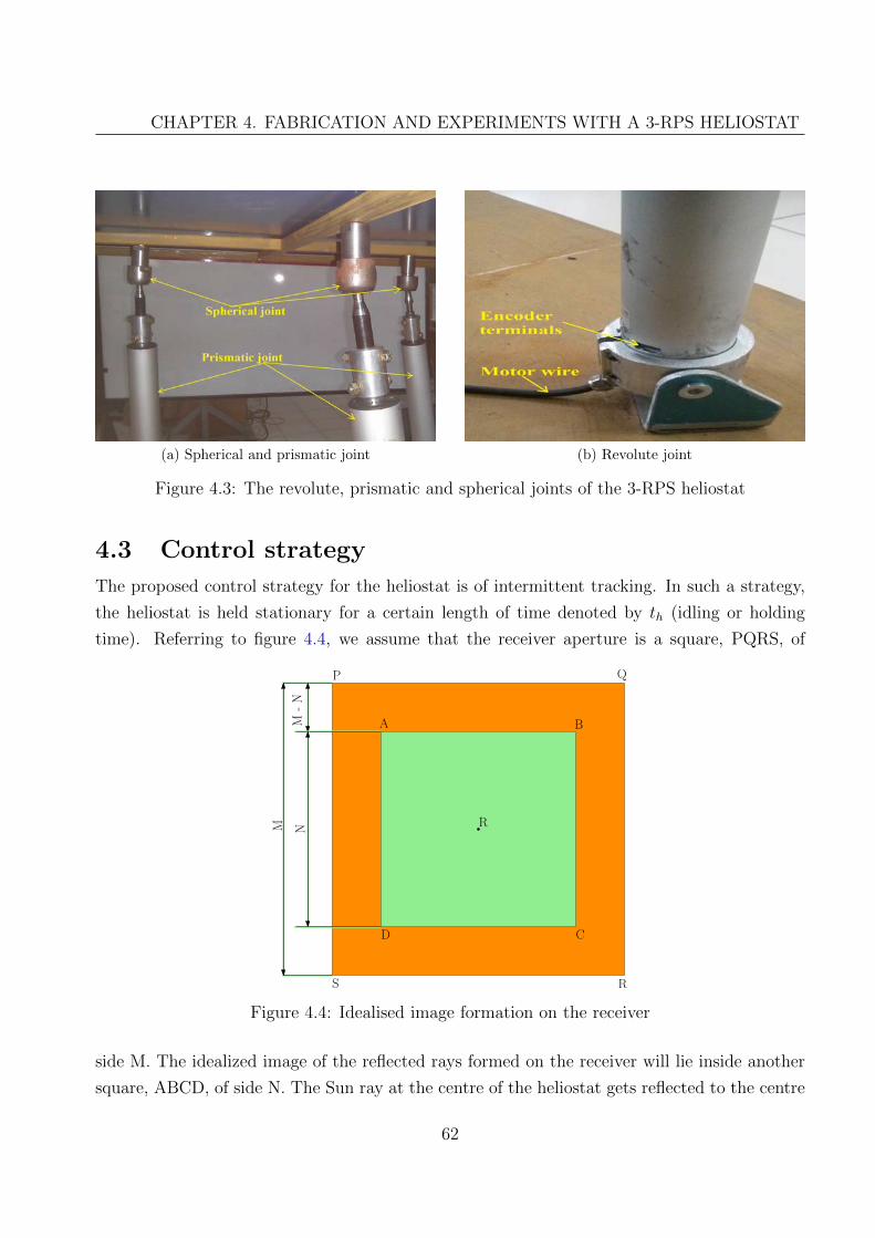
CHAPTER 4. FABRICATION AND EXPERIMENTS WITH A 3-RPS HELIOSTAT
(a) Spherical and prismatic joint (b) Revolute joint
Figure 4.3: The revolute, prismatic and spherical joints of the 3-RPS heliostat
4.3 Control strategy
The proposed control strategy for the heliostat is of intermittent tracking. In such a strategy,
the heliostat is held stationary for a certain length of time denoted by th (idling or holding
time). Referring to figure 4.4, we assume that the receiver aperture is a square, PQRS, of
P Q
RS
A B
CD
RM NM
-N
Figure 4.4: Idealised image formation on the receiver
side M. The idealized image of the reflected rays formed on the receiver will lie inside another
square, ABCD, of side N. The Sun ray at the centre of the heliostat gets reflected to the centre
62
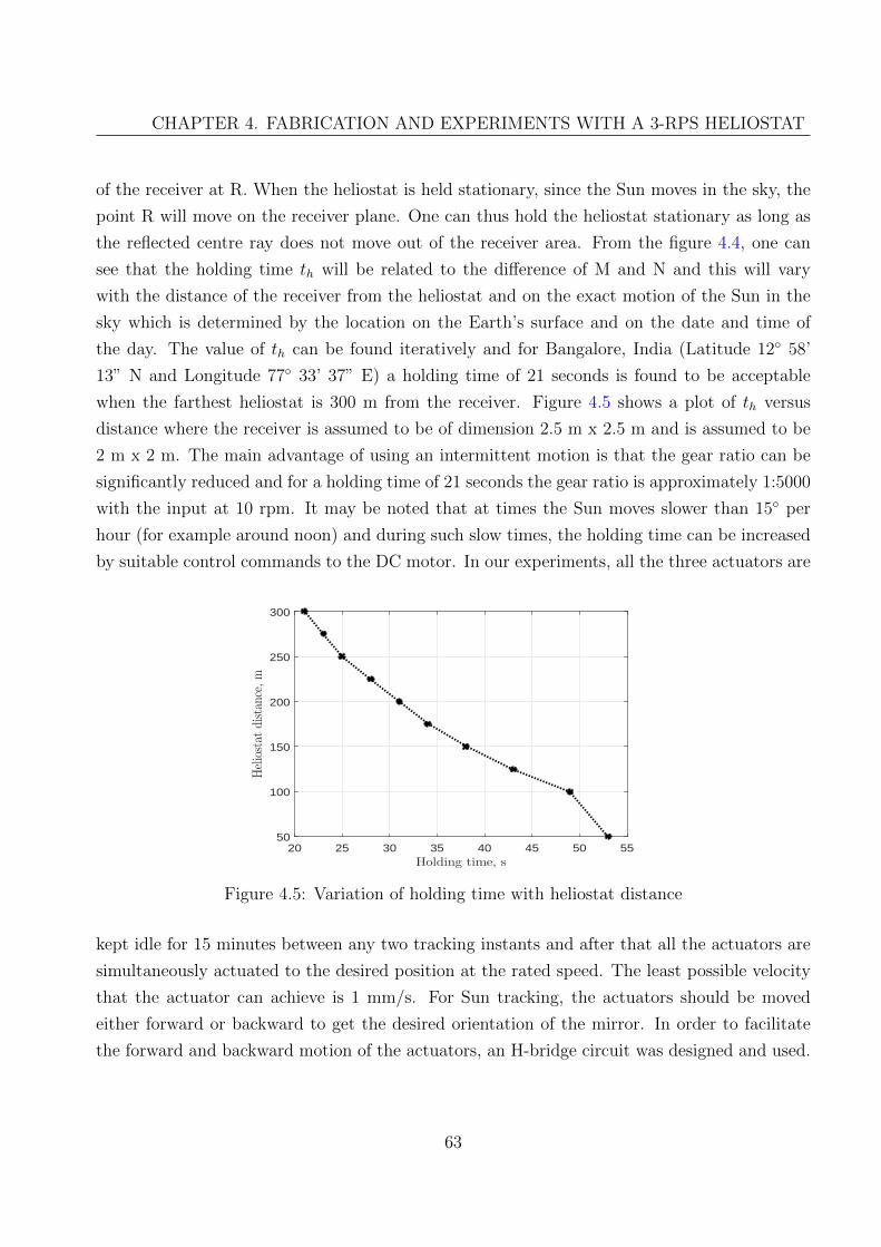
CHAPTER 4. FABRICATION AND EXPERIMENTS WITH A 3-RPS HELIOSTAT
of the receiver at R. When the heliostat is held stationary, since the Sun moves in the sky, the
point R will move on the receiver plane. One can thus hold the heliostat stationary as long as
the reflected centre ray does not move out of the receiver area. From the figure 4.4, one can
see that the holding time th will be related to the difference of M and N and this will vary
with the distance of the receiver from the heliostat and on the exact motion of the Sun in the
sky which is determined by the location on the Earth’s surface and on the date and time of
the day. The value of th can be found iteratively and for Bangalore, India (Latitude 12◦ 58’
13” N and Longitude 77◦ 33’ 37” E) a holding time of 21 seconds is found to be acceptable
when the farthest heliostat is 300 m from the receiver. Figure 4.5 shows a plot of th versus
distance where the receiver is assumed to be of dimension 2.5 m x 2.5 m and is assumed to be
2 m x 2 m. The main advantage of using an intermittent motion is that the gear ratio can be
significantly reduced and for a holding time of 21 seconds the gear ratio is approximately 1:5000
with the input at 10 rpm. It may be noted that at times the Sun moves slower than 15◦ per
hour (for example around noon) and during such slow times, the holding time can be increased
by suitable control commands to the DC motor. In our experiments, all the three actuators are
20 25 30 35 40 45 50 55
Holding time, s
50
100
150
200
250
300
Heliostat
distance,m
Figure 4.5: Variation of holding time with heliostat distance
kept idle for 15 minutes between any two tracking instants and after that all the actuators are
simultaneously actuated to the desired position at the rated speed. The least possible velocity
that the actuator can achieve is 1 mm/s. For Sun tracking, the actuators should be moved
either forward or backward to get the desired orientation of the mirror. In order to facilitate
the forward and backward motion of the actuators, an H-bridge circuit was designed and used.
63

CHAPTER 4. FABRICATION AND EXPERIMENTS WITH A 3-RPS HELIOSTAT
4.3.1 H bridge
A motor driver circuit or an H-bridge is shown in figure 4.6. The H-bridge helps to drive
the actuators forward and backward [89, 90]. For the H-bridge, two P type power MOSFETs
Figure 4.6: Schematic of the H-bridge circuit for an actuator
(IRF4905) and two N type power MOSFETs (IRF3205) are used. There are two Pulse Width
Modulation (PWM) input ports and a digital pin to switch on the power MOSFET 2N7000.
At a time, only one of the two power MOSFETs, 2N7000, will be switched on. For this to
happen, a logical NOT gate, IC 7404, is connected between the two 2N7000 MOSFETs. A
current sensor, ACS712, is connected in series with the motor to cut off the supply in case some
excess current passes through the motor. The H-bridge implemented on a printed circuit board
for all the three actuators is shown in figure 4.7. The supply voltage for the actuators is 24 V
and the maximum rated current is 3.5 A.
4.3.2 The microcontroller
ATMEGA2560 micro-controller is used to provide the PWM signals, turn on digital PIN 1 and
for reading the encoder output. It is an 8-bit microcontroller capable of operating at 16 MHz
and is also one of the cheapest micro-controllers which could read data from all the three linear
actuator encoders simultaneously. From figure 4.6, when PIN 1 is turned on using digital input
from ATMEGA2560, current flows through the path ABEF and the actuator moves forward.
When PIN 1 is turned off, current flows through the path DEBC and the actuator moves
64
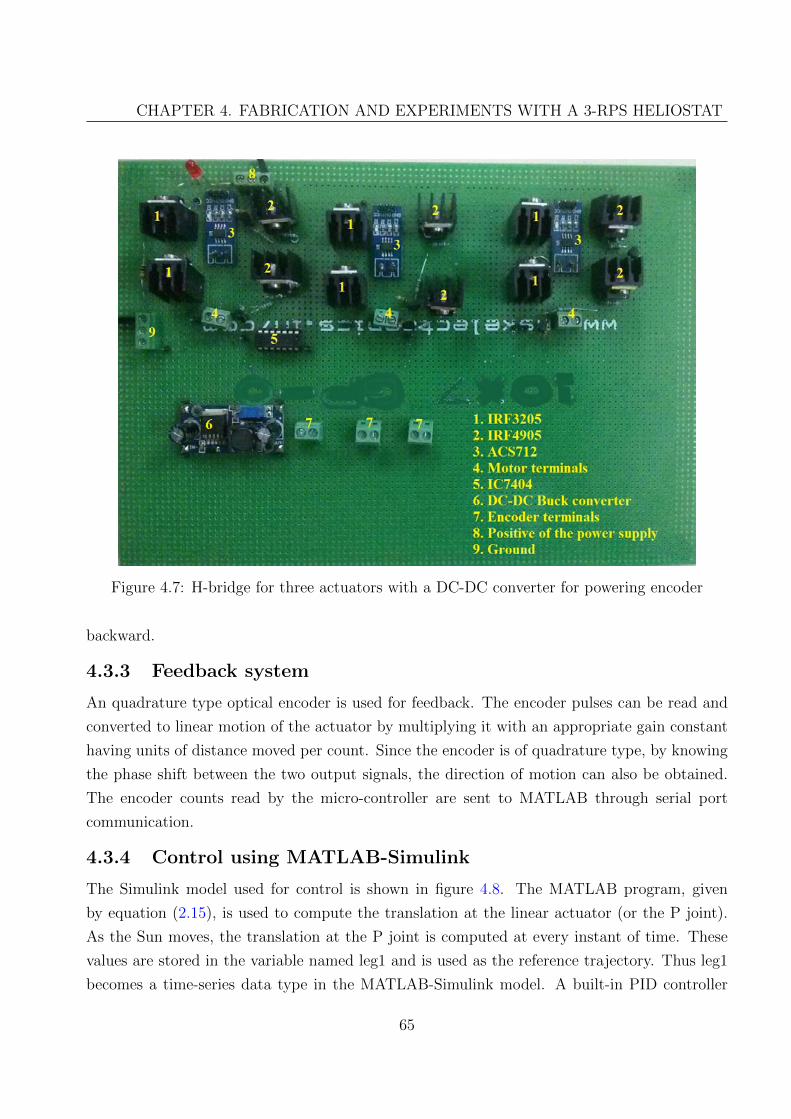
CHAPTER 4. FABRICATION AND EXPERIMENTS WITH A 3-RPS HELIOSTAT
Figure 4.7: H-bridge for three actuators with a DC-DC converter for powering encoder
backward.
4.3.3 Feedback system
An quadrature type optical encoder is used for feedback. The encoder pulses can be read and
converted to linear motion of the actuator by multiplying it with an appropriate gain constant
having units of distance moved per count. Since the encoder is of quadrature type, by knowing
the phase shift between the two output signals, the direction of motion can also be obtained.
The encoder counts read by the micro-controller are sent to MATLAB through serial port
communication.
4.3.4 Control using MATLAB-Simulink
The Simulink model used for control is shown in figure 4.8. The MATLAB program, given
by equation (2.15), is used to compute the translation at the linear actuator (or the P joint).
As the Sun moves, the translation at the P joint is computed at every instant of time. These
values are stored in the variable named leg1 and is used as the reference trajectory. Thus leg1
becomes a time-series data type in the MATLAB-Simulink model. A built-in PID controller
65
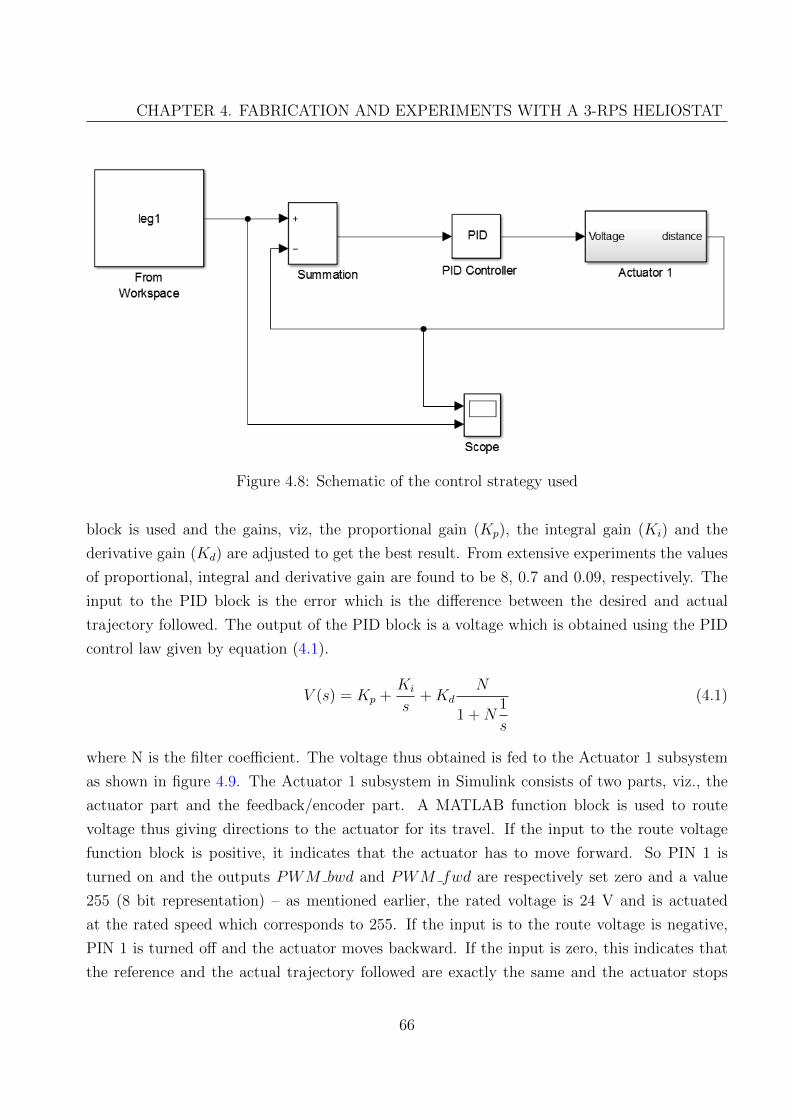
CHAPTER 4. FABRICATION AND EXPERIMENTS WITH A 3-RPS HELIOSTAT
Figure 4.8: Schematic of the control strategy used
block is used and the gains, viz, the proportional gain (Kp), the integral gain (Ki) and the
derivative gain (Kd) are adjusted to get the best result. From extensive experiments the values
of proportional, integral and derivative gain are found to be 8, 0.7 and 0.09, respectively. The
input to the PID block is the error which is the difference between the desired and actual
trajectory followed. The output of the PID block is a voltage which is obtained using the PID
control law given by equation (4.1).
V (s) = Kp +Ki
s+Kd
N
1 +N1
s
(4.1)
where N is the filter coefficient. The voltage thus obtained is fed to the Actuator 1 subsystem
as shown in figure 4.9. The Actuator 1 subsystem in Simulink consists of two parts, viz., the
actuator part and the feedback/encoder part. A MATLAB function block is used to route
voltage thus giving directions to the actuator for its travel. If the input to the route voltage
function block is positive, it indicates that the actuator has to move forward. So PIN 1 is
turned on and the outputs PWM bwd and PWM fwd are respectively set zero and a value
255 (8 bit representation) – as mentioned earlier, the rated voltage is 24 V and is actuated
at the rated speed which corresponds to 255. If the input is to the route voltage is negative,
PIN 1 is turned off and the actuator moves backward. If the input is zero, this indicates that
the reference and the actual trajectory followed are exactly the same and the actuator stops
66
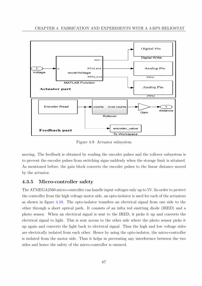
CHAPTER 4. FABRICATION AND EXPERIMENTS WITH A 3-RPS HELIOSTAT
Figure 4.9: Actuator subsystem
moving. The feedback is obtained by reading the encoder pulses and the rollover subsystem is
to prevent the encoder pulses from switching signs suddenly when the storage limit is attained.
As mentioned before, the gain block converts the encoder pulses to the linear distance moved
by the actuator.
4.3.5 Micro-controller safety
The ATMEGA2560 micro-controller can handle input voltages only up to 5V. In-order to protect
the controller from the high voltage motor side, an opto-isolator is used for each of the actuators
as shown in figure 4.10. The opto-isolator transfers an electrical signal from one side to the
other through a short optical path. It consists of an infra red emitting diode (IRED) and a
photo sensor. When an electrical signal is sent to the IRED, it picks it up and converts the
electrical signal to light. This is sent across to the other side where the photo sensor picks it
up again and converts the light back to electrical signal. Thus the high and low voltage sides
are electrically isolated from each other. Hence by using the opto-isolator, the micro-controller
is isolated from the motor side. Thus it helps in preventing any interference between the two
sides and hence the safety of the micro-controller is ensured.
67
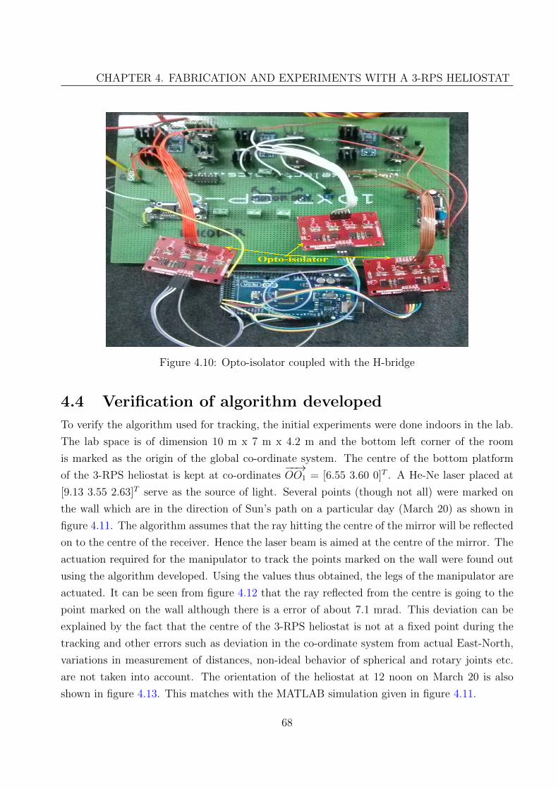
CHAPTER 4. FABRICATION AND EXPERIMENTS WITH A 3-RPS HELIOSTAT
Figure 4.10: Opto-isolator coupled with the H-bridge
4.4 Verification of algorithm developed
To verify the algorithm used for tracking, the initial experiments were done indoors in the lab.
The lab space is of dimension 10 m x 7 m x 4.2 m and the bottom left corner of the room
is marked as the origin of the global co-ordinate system. The centre of the bottom platform
of the 3-RPS heliostat is kept at co-ordinates−−→OO1 = [6.55 3.60 0]T . A He-Ne laser placed at
[9.13 3.55 2.63]T serve as the source of light. Several points (though not all) were marked on
the wall which are in the direction of Sun’s path on a particular day (March 20) as shown in
figure 4.11. The algorithm assumes that the ray hitting the centre of the mirror will be reflected
on to the centre of the receiver. Hence the laser beam is aimed at the centre of the mirror. The
actuation required for the manipulator to track the points marked on the wall were found out
using the algorithm developed. Using the values thus obtained, the legs of the manipulator are
actuated. It can be seen from figure 4.12 that the ray reflected from the centre is going to the
point marked on the wall although there is a error of about 7.1 mrad. This deviation can be
explained by the fact that the centre of the 3-RPS heliostat is not at a fixed point during the
tracking and other errors such as deviation in the co-ordinate system from actual East-North,
variations in measurement of distances, non-ideal behavior of spherical and rotary joints etc.
are not taken into account. The orientation of the heliostat at 12 noon on March 20 is also
shown in figure 4.13. This matches with the MATLAB simulation given in figure 4.11.
68

CHAPTER 4. FABRICATION AND EXPERIMENTS WITH A 3-RPS HELIOSTAT
Figure 4.11: MATLAB simulation of the Sun path in lab
Figure 4.12: Algorithm verification by tracking point
69
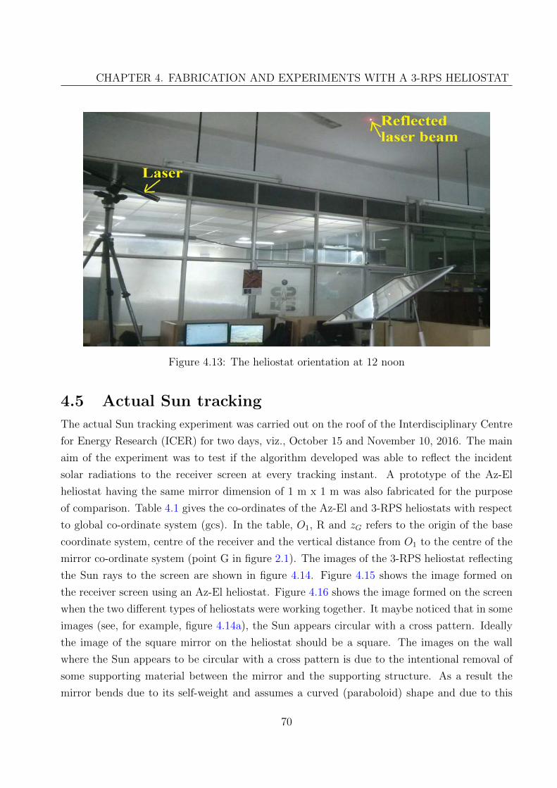
CHAPTER 4. FABRICATION AND EXPERIMENTS WITH A 3-RPS HELIOSTAT
Figure 4.13: The heliostat orientation at 12 noon
4.5 Actual Sun tracking
The actual Sun tracking experiment was carried out on the roof of the Interdisciplinary Centre
for Energy Research (ICER) for two days, viz., October 15 and November 10, 2016. The main
aim of the experiment was to test if the algorithm developed was able to reflect the incident
solar radiations to the receiver screen at every tracking instant. A prototype of the Az-El
heliostat having the same mirror dimension of 1 m x 1 m was also fabricated for the purpose
of comparison. Table 4.1 gives the co-ordinates of the Az-El and 3-RPS heliostats with respect
to global co-ordinate system (gcs). In the table, O1, R and zG refers to the origin of the base
coordinate system, centre of the receiver and the vertical distance from O1 to the centre of the
mirror co-ordinate system (point G in figure 2.1). The images of the 3-RPS heliostat reflecting
the Sun rays to the screen are shown in figure 4.14. Figure 4.15 shows the image formed on
the receiver screen using an Az-El heliostat. Figure 4.16 shows the image formed on the screen
when the two different types of heliostats were working together. It maybe noticed that in some
images (see, for example, figure 4.14a), the Sun appears circular with a cross pattern. Ideally
the image of the square mirror on the heliostat should be a square. The images on the wall
where the Sun appears to be circular with a cross pattern is due to the intentional removal of
some supporting material between the mirror and the supporting structure. As a result the
mirror bends due to its self-weight and assumes a curved (paraboloid) shape and due to this
70
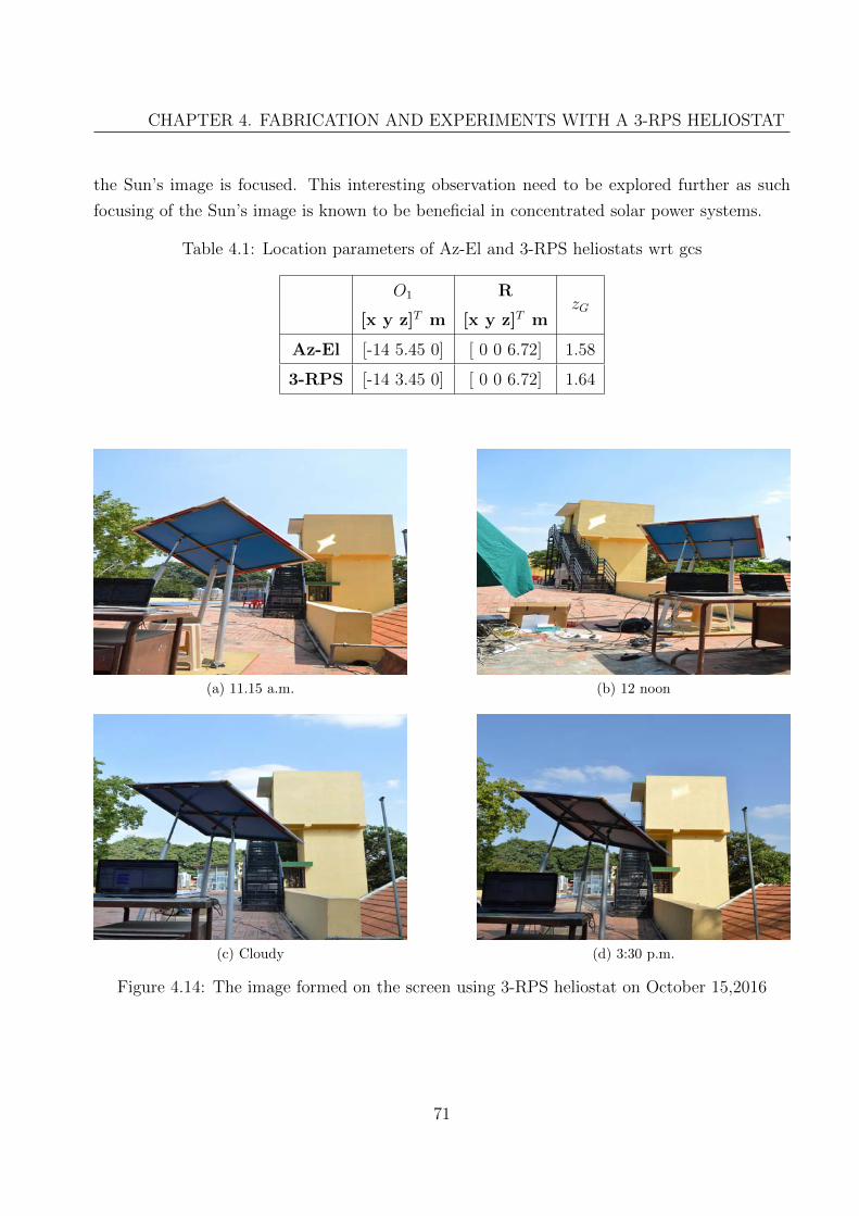
CHAPTER 4. FABRICATION AND EXPERIMENTS WITH A 3-RPS HELIOSTAT
the Sun’s image is focused. This interesting observation need to be explored further as such
focusing of the Sun’s image is known to be beneficial in concentrated solar power systems.
Table 4.1: Location parameters of Az-El and 3-RPS heliostats wrt gcs
O1
[x y z]T m
R
[x y z]T mzG
Az-El [-14 5.45 0] [ 0 0 6.72] 1.58
3-RPS [-14 3.45 0] [ 0 0 6.72] 1.64
(a) 11.15 a.m. (b) 12 noon
(c) Cloudy (d) 3:30 p.m.
Figure 4.14: The image formed on the screen using 3-RPS heliostat on October 15,2016
71

CHAPTER 4. FABRICATION AND EXPERIMENTS WITH A 3-RPS HELIOSTAT
(a) 09:30 a.m. (b) 12 noon
(c) Cloudy (d) 3:30 p.m.
Figure 4.15: The image formed on the screen using Az-El heliostat on October 15,2016
(a) 11:15 a.m. (b) 12 noon
(c) Almost cloudy (d) 3:30 p.m.
Figure 4.16: The image formed on the screen when Az-El and 3-RPS were working together onOctober 15,2016
72
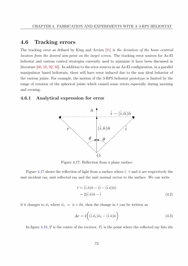
CHAPTER 4. FABRICATION AND EXPERIMENTS WITH A 3-RPS HELIOSTAT
4.6 Tracking errors
The tracking error as defined by King and Arvizu [91] is the deviation of the beam centroid
location from the desired aim-point on the target screen. The tracking error sources for Az-El
heliostat and various control strategies currently used to minimize it have been discussed in
literature [60, 58, 92, 93]. In addition to the error sources in an Az-El configuration, in a parallel
manipulator based heliostats, there will have error induced due to the non ideal behavior of
the various joints. For example, the motion of the 3-RPS heliostat prototype is limited by the
range of rotation of the spherical joints which caused some errors especially during morning
and evening.
4.6.1 Analytical expression for error
ir
n
(i.n)n
i− (i.n)n
O
θ θ
Figure 4.17: Reflection from a plane surface
Figure 4.17 shows the reflection of light from a surface where i, r and n are respectively the
unit incident ray, unit reflected ray and the unit normal vector to the surface. We can write
r = (i.n)n− (i− (i.n)n)
= 2(i.n)n− i (4.2)
if n changes to n1 where n1 = n+ δn, then the change in r can be written as
∆r = 2
((i.n1)n1 − (i.n)n
)(4.3)
In figure 4.18, P is the centre of the receiver, P1 is the point where the reflected ray hits the
73

CHAPTER 4. FABRICATION AND EXPERIMENTS WITH A 3-RPS HELIOSTAT
G
P
P1
O
NS
in
r1
r
XY
Z
N1
n1
∆r
Figure 4.18: Tracking error
receiver when errors are present, G is the centre of the reflector. We can write
−→OG+ C1r =
−→OP
−→OG+ C1r1 =
−→OP 1
C1∆r =−→OP 1 −
−→OP
2C1
((i.n1)n1 − (i.n)n
)=−→OP 1 −
−→OP =
∆x
∆y
∆z
(4.4)
where C1 is a constant and also the errors are assumed to be small.
For Az-El method, the incident ray and normals would be
i =
cosαs cosφs
cosαs sinφs
sinαs
; n =
cosαn cosφn
cosαn sinφn
sinαn
; n1 =
cos(αn + ∆αn) cos(φn + ∆φn)
cos(αn + ∆αn) sin(φn + ∆φn)
sin(αn + ∆αn)
where α and φ are the elevation (measured from ground plane) and azimuth (measured from
X axis) angles of the Sun vector and normal indicated by the suffixes s and n respectively.
For the 3-RPS, in terms of the joint space variables, the coordinates of the spherical joints
74
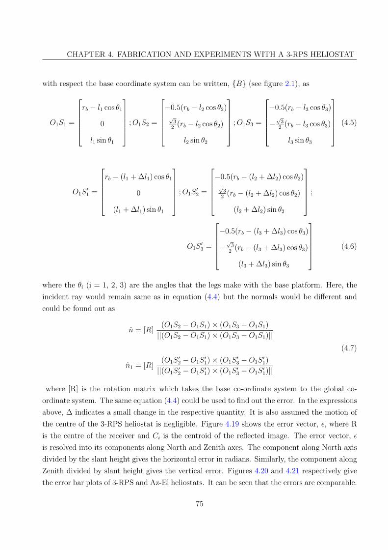
CHAPTER 4. FABRICATION AND EXPERIMENTS WITH A 3-RPS HELIOSTAT
with respect the base coordinate system can be written, {B} (see figure 2.1), as
O1S1 =
rb − l1 cos θ1
0
l1 sin θ1
;O1S2 =
−0.5(rb − l2 cos θ2)√32
(rb − l2 cos θ2)
l2 sin θ2
;O1S3 =
−0.5(rb − l3 cos θ3)
−√32
(rb − l3 cos θ3)
l3 sin θ3
(4.5)
O1S′1 =
rb − (l1 + ∆l1) cos θ1
0
(l1 + ∆l1) sin θ1
;O1S′2 =
−0.5(rb − (l2 + ∆l2) cos θ2)√32
(rb − (l2 + ∆l2) cos θ2)
(l2 + ∆l2) sin θ2
;
O1S′3 =
−0.5(rb − (l3 + ∆l3) cos θ3)
−√32
(rb − (l3 + ∆l3) cos θ3)
(l3 + ∆l3) sin θ3
(4.6)
where the θi (i = 1, 2, 3) are the angles that the legs make with the base platform. Here, the
incident ray would remain same as in equation (4.4) but the normals would be different and
could be found out as
n = [R](O1S2 −O1S1)× (O1S3 −O1S1)
||(O1S2 −O1S1)× (O1S3 −O1S1)||(4.7)
n1 = [R](O1S
′2 −O1S
′1)× (O1S
′3 −O1S
′1)
||(O1S ′2 −O1S ′1)× (O1S ′3 −O1S ′1)||
where [R] is the rotation matrix which takes the base co-ordinate system to the global co-
ordinate system. The same equation (4.4) could be used to find out the error. In the expressions
above, ∆ indicates a small change in the respective quantity. It is also assumed the motion of
the centre of the 3-RPS heliostat is negligible. Figure 4.19 shows the error vector, ε, where R
is the centre of the receiver and Ci is the centroid of the reflected image. The error vector, ε
is resolved into its components along North and Zenith axes. The component along North axis
divided by the slant height gives the horizontal error in radians. Similarly, the component along
Zenith divided by slant height gives the vertical error. Figures 4.20 and 4.21 respectively give
the error bar plots of 3-RPS and Az-El heliostats. It can be seen that the errors are comparable.
75
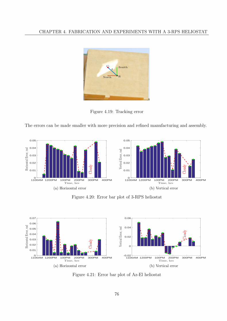
CHAPTER 4. FABRICATION AND EXPERIMENTS WITH A 3-RPS HELIOSTAT
Zenith
North
ǫ
R
Ci
Figure 4.19: Tracking error
The errors can be made smaller with more precision and refined manufacturing and assembly.
1100AM 1200PM 100PM 200PM 300PM 400PM
Time, hrs
0
0.01
0.02
0.03
0.04
0.05
Horizon
talE
rror,r
ad
Cloud
y
(a) Horizontal error
1100AM 1200PM 100PM 200PM 300PM 400PM
Time, hrs
0
0.01
0.02
0.03
0.04
0.05
VerticalE
rror,r
ad
Cloud
y(b) Vertical error
Figure 4.20: Error bar plot of 3-RPS heliostat
1100AM 1200PM 100PM 200PM 300PM 400PM
Time, hrs
0
0.01
0.02
0.03
0.04
0.05
0.06
0.07
Horizon
talE
rror,r
ad
Cloud
y
(a) Horizontal error
1100AM 1200PM 100PM 200PM 300PM 400PM
Time, hrs
-0.02
0
0.02
0.04
0.06
VerticalE
rror,r
ad
Cloud
y
(b) Vertical error
Figure 4.21: Error bar plot of Az-El heliostat
76
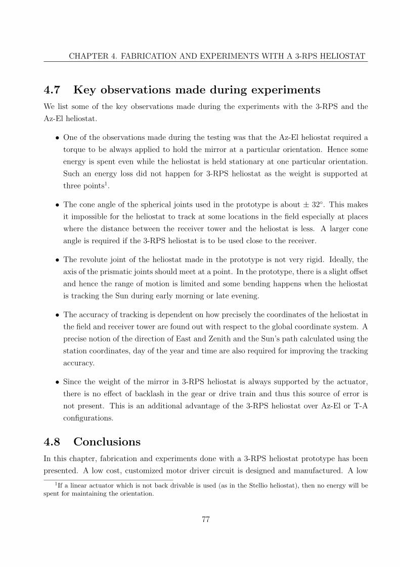
CHAPTER 4. FABRICATION AND EXPERIMENTS WITH A 3-RPS HELIOSTAT
4.7 Key observations made during experiments
We list some of the key observations made during the experiments with the 3-RPS and the
Az-El heliostat.
• One of the observations made during the testing was that the Az-El heliostat required a
torque to be always applied to hold the mirror at a particular orientation. Hence some
energy is spent even while the heliostat is held stationary at one particular orientation.
Such an energy loss did not happen for 3-RPS heliostat as the weight is supported at
three points1.
• The cone angle of the spherical joints used in the prototype is about ± 32◦. This makes
it impossible for the heliostat to track at some locations in the field especially at places
where the distance between the receiver tower and the heliostat is less. A larger cone
angle is required if the 3-RPS heliostat is to be used close to the receiver.
• The revolute joint of the heliostat made in the prototype is not very rigid. Ideally, the
axis of the prismatic joints should meet at a point. In the prototype, there is a slight offset
and hence the range of motion is limited and some bending happens when the heliostat
is tracking the Sun during early morning or late evening.
• The accuracy of tracking is dependent on how precisely the coordinates of the heliostat in
the field and receiver tower are found out with respect to the global coordinate system. A
precise notion of the direction of East and Zenith and the Sun’s path calculated using the
station coordinates, day of the year and time are also required for improving the tracking
accuracy.
• Since the weight of the mirror in 3-RPS heliostat is always supported by the actuator,
there is no effect of backlash in the gear or drive train and thus this source of error is
not present. This is an additional advantage of the 3-RPS heliostat over Az-El or T-A
configurations.
4.8 Conclusions
In this chapter, fabrication and experiments done with a 3-RPS heliostat prototype has been
presented. A low cost, customized motor driver circuit is designed and manufactured. A low
1If a linear actuator which is not back drivable is used (as in the Stellio heliostat), then no energy will bespent for maintaining the orientation.
77
CHAPTER 4. FABRICATION AND EXPERIMENTS WITH A 3-RPS HELIOSTAT
cost controller was made using a widely available ATMEGA2560 board and a PID controller was
implemented to control the orientation of the heliostat at desired instants of time. The micro-
controller and the motor side are properly isolated using an opto-isolator for safety reasons. The
algorithm developed for tracking the Sun in chapter 2 is verified first in the lab and then the
actual Sun tracking is carried out outdoors. It is shown that 3-RPS heliostat is able to track the
Sun and focus the incident solar radiation on a wall chosen as the receiver screen. It is shown
that the tracking error is comparable to that obtained from a traditional Azimuth-Elevation
configuration heliostat. Thus it is demonstrated that the proposed 3-RPS manipulator can
indeed work as a heliostat in a CR solar thermal system.
78

Chapter 5
Conclusions and Future work
5.1 Summary
This thesis is an attempt to improve the current Sun tracking methods employed in concentrated
solar power stations by moving from serial mechanisms to parallel mechanisms. The main
reasons for such a change is the inherent advantages, such as high stiffness, large load carrying
capacity, high accuracy in positioning and orienting the end effector, easy to obtain inverse
kinematics and ease of real time control available in parallel mechanisms over serial mechanisms.
In chapter 1, the motivation and a detailed literary survey on the approaches to harvest solar
energy, existing Sun tracking methods, and sources of tracking errors are discussed. It is shown
that most common heliostats used in concentrated solar power systems use a serial mechanism
and they are the Azimuth-Elevation and the Target-Aligned configurations. The chapter ends
with the scope and contribution of the thesis.
Chapter 2 presents the over-view of various Sun tracking approaches using parallel manip-
ulators. The currently used parallel manipulators cannot be used in a CR system since it is
difficult to find the reference point on the moving platform which is very important for the
calculation of transformation matrix and to obtain motion planning algorithms. Two potential
parallel manipulators, each with three actuators, are identified for replacing the serial chains
used in central receiver systems. These are the 3-RPS and 3-UPU wrist manipulators. This
chapter also gives a detailed account of the development of tracking algorithms using the 3-UPU
wrist and 3-RPS manipulators by solving the inverse kinematics. A simulation study of the
two proposed parallel manipulators is carried out and found that there are certain drawbacks,
such as leg intersection and precise manufacturing required to get a fixed point, for the 3-UPU
wrist.
Chapter 3 discusses the structural design of heliostats. A finite element analysis based
79

CHAPTER 5. CONCLUSIONS AND FUTURE WORK
approach is used to model and analyze the heliostat with a goal of finding the most optimum
structure of a heliostat to withstand loading due to wind and self-weight. For the operating
wind load of 10 m/s and 22 m/s, an iterative search is carried out to find the optimal values of
certain design parameters which would help in achieving a stroke of 700 mm for the actuators to
track the Sun and to obtain the least weight of the supporting structure. It is shown that when
larger mirrors, such as 5m x 5m mirrors, are used the saving in structure in the parallel 3-RPS
configuration is as high as 65% when compared to the traditional serial Azimuth-Elevation and
Target-Aligned configurations.
Chapter 4 deals with the detailed design and fabrication of the 3-RPS heliostat. This chapter
also gives a detailed description of the motor driver circuit, the control strategy implemented
using MATLAB-Simulink and ATMEGA2560 and verification of algorithm by tracking points
marked on the wall. An actual Sun-tracking experiment is also carried out on the roof of a
building and the tracking errors are quantified for both Az-El and 3-RPS heliostats. It is shown
that the tracking errors are comparable and the 3-RPS parallel manipulator could be used as
a heliostat in central receiver systems.
5.2 Scope for future work
The approach and the results reported in this work can be extended in several ways. We list
some of the main ones below.
• The value of Z displacement in the 3-RPS heliostat zG (in equation (2.2)), is chosen
arbitrarily as it is a free variable. It is possible to use this redundancy to optimize
the motion of the heliostat such that some objective function is minimized. We have
attempted to reduce cosine losses during Sun tracking by changing zG. However, this
effect is very small as the range of zG is limited by the maximum stroke of the linear
actuators.
• Simulation study for the 3-RPS were carried out for equinoxes and solstices. There is
a scope to carry out the simulation study for one whole year and see if there are any
variations in the results presented in chapter 2. Rajasthan and Bangalore are the only
two locations that were considered for the simulation study and it would be useful to do
simulations for various other latitudes.
• A more elaborate simulation study has to be carried out for 3-UPU wrist especially to see
if the legs intersect and to what angle it has to be rotated initially. The 3-UPU wrist has
certain shortcomings as mentioned in section 2.6. However, it has the appealing property
80

CHAPTER 5. CONCLUSIONS AND FUTURE WORK
of being ‘software switchable’ between Az-El and T-A or any other two successive rotation
configuration. Hence, it would be worthwhile to design and manufacture a prototype and
perform experiments with it.
• The observations made in section 4.7 have to be reworked especially related to the range
of motion of the spherical joints and the prismatic joint axes. The actual Sun tracking
on the roof is carried out from 11:15 am to 3:30 pm. The experiment takes a lot of time
to set-up the mirror, controllers and computers. The surrounding trees also block the
sunlight beyond 3:30 pm. The max slant length (distance from the mirror centre to the
centre of the receiver) is less than 16 m and the relative height between the mirror centre
and the receiver centre is only 5.08 m. Due to this the spherical joints try to rotate more
than its allowed range and cause some bending of the actuators and noise. All these
difficulties suggest more experiments with proper facilities to obtain better quantitative
results in Sun tracking error and performance of the 3-RPS based heliostat.
• The first generation prototype done in this thesis could only quantify the tracking errors.
The tracking errors are quite high, the average being 30 mrad for 3-RPS heliostat. This
aspect needs to be reworked with more refined manufacturing and more robust control
strategy. The target for the second generation 3-RPS heliostats would be to have a
tracking error of less than 2 mrad. To ensure this, two methods are suggested and these
are:
1. Self-calibrating controllers
This idea is from the work carried out by Baheti and Scott [54]. Here the main
assumption made is that the centre of the 3-RPS heliostat(point G in figure 2.1)
moves very less compared to the other dimensions. This is verified from the figures 2.8
and 2.9 in section 2.3.5 and is a reasonable assumption. From the images captured (
for eg. figure 4.19), the error vector can be calculated. From this the ideal reflected
ray (the ray which should have hit the centre of the receiver) and the actual reflected
ray (the ray which hits the centroid of the reflected image) can be calculated. From
the notion of the reflected ray, the normal to the mirror (both ideal and actual) can be
determined (equation (1.4)). The error in normal, εn, would be the difference between
the two and can be given as the product of a skew-symmetric matrix and a parameter
matrix which is to be estimated. The elements of the skew-symmetric matrix are
the direction cosines of the Sun vector. Since the skew-symmetric matrix is singular,
some other approaches have to be used to evaluate the parameter matrix. One such
81
CHAPTER 5. CONCLUSIONS AND FUTURE WORK
possibility is the use of singular value decomposition (SVD) to get an estimate of the
parameters . This can be used to find the rotation matrix and hence the leg-length
as described by equation (2.15). With the modern computing techniques available,
a live correction using a camera and SVD can be employed to minimize the tracking
error at every tracking instant.
2. Optimization based control
The problem of error correction can also be posed as a distance minimization op-
timization problem where the distance between the centroid of reflected image and
receiver centre is to be minimized. By doing so, elements of the rotation matrix
which would minimize the distance, CiR (in figure 4.19) can be found out and hence
the corrections in the actuations required. This method also requires an on board
computer and camera.
82

Appendix
A MATLAB program for calculating sun angles
function [elevation, azimuth]=alpha-azimuthcalc(LT,d,longitude,latitude)
% LT=local time in seconds, % d is the number of days since the start of the year
% longitude of the place in degrees, East is positive and west is negative
% latitude of the place in degrees, North is positive and south is negative
LSTM = 15*5.5 ;% (in degrees) local standard time meridian. 5.5 is the time differance
between local time for india and GMT
B=60*(d-81)/365; % in degrees
EOT=9.87*sind(2*B)-7.53*cosd(B)-1.5*sind(B); % in minutes
TC=4*(longitude-LSTM)+EOT; % Time Correction Factor (TC) in minutes
LST=LT./3600+TC/60; % in hours
HRA=15*(LST-12); % hour angle in degrees
delta=23.45*sind(B); % declination angle in degrees
elevation=asind(sind(delta)*sind(latitude)+cosd(delta)*cosd(latitude).*cosd(HRA));
a1=sind(delta)*cosd(latitude);
a2=cosd(delta)*sind(latitude);
a=acosd((a1-a2.*cosd(HRA))./cosd(elevation));
for i=1:length(HRA)
if (HRA(i)≤0 )
azimuth(i)=a(i);
elseif( 116 ≤ d && d ≤ 229 && HRA(i)¿0)
azimuth(i) = -a(i);
else
azimuth(i) = 360-a(i);
end end end
83
Bibliography
[1] NREL. India Solar Resource. url: http://www.nrel.gov/international/images/
india_dni_annual.jpg (cit. on p. 1).
[2] Atul Sharma. “A comprehensive study of solar power in India and World”. In: Renewable
and Sustainable Energy Reviews 15.4 (2011), pp. 1767 –1776. issn: 1364-0321 (cit. on
p. 1).
[3] W Schiel and T Keck. “Concentrating solar power technology: Principles, developments
and applications”. In: Concentrating solar power technology: principles, developments and
applications. Ed. by Keith Lovegrove and Wes Stein. Cambridge, UK: Woodhead Pub-
lishing, 2012. Chap. 9, pp. 284–322 (cit. on p. 1).
[4] K. Lovegrove and J. Pye. “Fundamental principles of concentrating solar power (CSP)
systems”. In: Concentrating Solar Power Technology. Ed. by Keith Lovegrove and Wes
Stein. Woodhead Publishing Series in Energy. Woodhead Publishing, 2012, pp. 16 –67.
isbn: 978-1-84569-769-3 (cit. on p. 2).
[5] SunShot Initiative. url: https://energy.gov/eere/sunshot/sunshot-initiative-
goals (cit. on p. 2).
[6] Gregory J Kolb, Roger Davenport, David Gorman, Ron Lumia, Robert Thomas, and
Matthew Donnelly. “Heliostat cost reduction”. In: ASME 2007 Energy Sustainability
Conference. American Society of Mechanical Engineers. 2007, pp. 1077–1084 (cit. on p. 2).
[7] Gregory J Kolb, Clifford K Ho, Thomas R Mancini, and Jesse A Gary. Power tower
technology roadmap and cost reduction plan. Tech. rep. Sandia National Laboratories,
Albuquerque, NM, 2011. url: http://prod.sandia.gov/techlib/access-control.
cgi/2011/112419.pdf (cit. on p. 2).
[8] NREL. National Renewable Energy Labarotary. url: http : / / www . nrel . gov / csp /
solarpaces/project\_detail.cfm/projectID=62 (cit. on p. 2).
84

BIBLIOGRAPHY
[9] J.B Blackmon. “Concentrating solar power technology: Principles, developments and ap-
plications”. In: Concentrating solar power technology: principles, developments and appli-
cations. Ed. by Keith Lovegrove and Wes Stein. Cambridge, UK: Woodhead Publishing,
2012. Chap. 17, pp. 536–576 (cit. on p. 2).
[10] PV EDUCATION. url: http://pveducation.org/pvcdrom/properties-of-sunlight/
elevation-angle (cit. on p. 3).
[11] Ibrahim Reda and Afshin Andreas. “Solar position algorithm for solar radiation applica-
tions”. In: Solar Energy 76.5 (2004), pp. 577–589 (cit. on p. 3).
[12] William B Stine and Michael Geyer. Power from the Sun. 2001. url: http://www.
powerfromthesun.net/book.html (cit. on p. 3).
[13] NOAA Sun Position Calculator. url: https : / / www . esrl . noaa . gov / gmd / grad /
solcalc/azel.html (cit. on p. 3).
[14] MATLAB. Natick, Massachusetts, 2012 (cit. on p. 4).
[15] US Department of Energy. url: https://www1.eere.energy.gov/solar/pdfs/solar_
timeline.pdf (cit. on pp. 5, 8).
[16] Zachary Alden Smith and Katrina D Taylor. Renewable and alternative energy resources:
a reference handbook. ABC-CLIO, 2008. isbn: 978-1-59884-089-6 (cit. on p. 5).
[17] Evangelos Bellos, Christos Tzivanidis, and Kimon A. Antonopoulos. “A detailed working
fluid investigation for solar parabolic trough collectors”. In: Applied Thermal Engineering
114 (2017), pp. 374 –386 (cit. on p. 6).
[18] L Salgado Conrado, A Rodriguez-Pulido, and G Calderon. “Thermal performance of
parabolic trough solar collectors”. In: Renewable and Sustainable Energy Reviews 67
(2017), pp. 1345–1359 (cit. on p. 6).
[19] E. Zarza Moya. “7 - Parabolic-trough concentrating solar power (CSP) systems”. In:
Concentrating Solar Power Technology. Ed. by Keith Lovegrove and Wes Stein. Woodhead
Publishing Series in Energy. Woodhead Publishing, 2012, pp. 197 –239. isbn: 978-1-84569-
769-3 (cit. on p. 6).
[20] Zhongzhu Qiu, Peng Li, Chunying Li, Qunzhi Zhu, Tao Zhang, and Chengyao Wang.
“A novel design concept for a reflector of parabolic trough concentrator based on pure
bending and correction principle”. In: Solar Energy 141 (2017), pp. 59–69 (cit. on p. 6).
85
BIBLIOGRAPHY
[21] S. Meiser, S. Schneider, E. Lupfert, B. Schiricke, and R. Pitz-Paal. “Evaluation and
assessment of gravity load on mirror shape and focusing quality of parabolic trough solar
mirrors using finite-element analysis”. In: Applied Energy 185 (2017). Clean, Efficient and
Affordable Energy for a Sustainable Future, pp. 1210 –1216 (cit. on p. 6).
[22] LL Vant-Hull. “Concentrating solar power technology: Principles, developments and ap-
plications”. In: Concentrating solar power technology: principles, developments and appli-
cations. Ed. by Keith Lovegrove and Wes Stein. Cambridge, UK: Woodhead Publishing,
2012. Chap. 8, pp. 240–283 (cit. on pp. 6, 10, 12).
[23] Roof-top solar installations for cooking. url: http://www.indiatimes.com/culture/
food/10-facts-about-indias-mega-kitchens-that-will-leave-you-stunned-
233823.html (cit. on p. 6).
[24] JJ Droher and SE Squier. Performance of the Vanguard Solar Dish-Stirling Engine Mod-
ule. Final report. Tech. rep. Rockwell International Corp., Canoga Park, CA (USA).
Energy Technology Engineering Center, 1986 (cit. on p. 6).
[25] Andrea Giostri and Ennio Macchi. “An advanced solution to boost sun-to-electricity
efficiency of parabolic dish”. In: Solar Energy 139 (2016), pp. 337–354 (cit. on p. 6).
[26] Charles E Andraka. “Dish Stirling advanced latent storage feasibility”. In: Energy Proce-
dia 49 (2014), pp. 684–693 (cit. on p. 7).
[27] C Lertsatitthanakorn, J Jamradloedluk, and M Rungsiyopas. “Electricity generation from
a solar parabolic concentrator coupled to a thermoelectric module”. In: Energy Procedia
52 (2014), pp. 150–158 (cit. on p. 7).
[28] USAID. Grid-Connected Renewable Energy: Solar Electric Technologies. url: http://
www.energytoolbox.org/gcre/mod_5/gcre_solar.pdf (cit. on p. 7).
[29] Haisheng Chen, Thang Ngoc Cong, Wei Yang, Chunqing Tan, Yongliang Li, and Yulong
Ding. “Progress in electrical energy storage system: A critical review”. In: Progress in
Natural Science 19.3 (2009), pp. 291 –312. issn: 1002-0071 (cit. on p. 7).
[30] H. Ibrahim, A. Ilinca, and J. Perron. “Energy storage systems—Characteristics and com-
parisons”. In: Renewable and Sustainable Energy Reviews 12.5 (2008), pp. 1221 –1250.
issn: 1364-0321 (cit. on p. 7).
[31] Belen Zalba, Jose M Marin, Luisa F. Cabeza, and Harald Mehling. “Review on thermal
energy storage with phase change: materials, heat transfer analysis and applications”. In:
Applied Thermal Engineering 23.3 (2003), pp. 251 –283. issn: 1359-4311 (cit. on p. 8).
86

BIBLIOGRAPHY
[32] GA Lane. Solar heat storage: Latent heat materials. Volume II. Technology. Tech. rep.
Dow Chemical Co., Midland, MI, 1986 (cit. on p. 8).
[33] A Haberle. “Concentrating solar power technology: Principles, developments and appli-
cations”. In: Concentrating solar power technology: principles, developments and appli-
cations. Ed. by Keith Lovegrove and Wes Stein. Cambridge, UK: Woodhead Publishing,
2012. Chap. 19, pp. 602–619 (cit. on p. 8).
[34] Abbas A Akhil, Georgianne Huff, Aileen B Currier, Benjamin C Kaun, Dan M Rastler,
Stella Bingqing Chen, Andrew L Cotter, Dale T Bradshaw, and William D Gauntlett.
DOE/EPRI 2013 electricity storage handbook in collaboration with NRECA. Sandia Na-
tional Laboratories Albuquerque, NM, USA, 2013 (cit. on p. 8).
[35] Michael Mendelsohn, Travis Lowder, and Brendan Canavan. Utility-Scale Concentrating
Solar Power and Photovoltaics Projects: A Technology and Market Overview. Tech. rep.
NREL Technical Report, NREL/TP-6A20-51137, 2012, pp. 275–3000. url: https://
www.nrel.gov/docs/fy12osti/51137.pdf (cit. on p. 8).
[36] A Cengel Yunus and A Boles Michael. Thermodynamics: An engineering approach. 2006.
isbn: 978-0073398174 (cit. on p. 8).
[37] FW Lipps and LL Vant-Hull. “A cellwise method for the optimization of large central
receiver systems”. In: Solar Energy 20.6 (1978), pp. 505–516 (cit. on p. 8).
[38] Hossein Mousazadeh, Alireza Keyhani, Arzhang Javadi, Hossein Mobli, Karen Abrinia,
and Ahmad Sharifi. “A review of principle and sun-tracking methods for maximizing solar
systems output”. In: Renewable and Sustainable Energy Reviews 13.8 (2009), pp. 1800–
1818 (cit. on p. 8).
[39] Chia-Yen Lee, Po-Cheng Chou, Che-Ming Chiang, and Chiu-Feng Lin. “Sun tracking
systems: a review”. In: Sensors 9.5 (2009), pp. 3875–3890 (cit. on p. 8).
[40] RB Ashith Shyam and A Ghosal. “Three-degree-of-freedom parallel manipulator to track
the sun for concentrated solar power systems”. In: Chinese Journal of Mechanical Engi-
neering 28.4 (2015), pp. 793–800 (cit. on p. 9).
[41] Eugene A Igel and Robert Lee Hughes. “Optical analysis of solar facility heliostats”. In:
Solar Energy 22.3 (1979), pp. 283–295 (cit. on p. 10).
[42] Harald Ries and Markus Schubnell. “The optics of a two-stage solar furnace”. In: Solar
Energy Materials 21.2 (1990), pp. 213–217 (cit. on p. 10).
87

BIBLIOGRAPHY
[43] R Zaibel, E Dagan, J Karni, and Harald Ries. “An astigmatic corrected target-aligned
heliostat for high concentration”. In: Solar Energy Materials and Solar Cells 37.2 (1995),
pp. 191–202 (cit. on p. 10).
[44] YT Chen, KK Chong, TP Bligh, LC Chen, Jasmy Yunus, KS Kannan, BH Lim, CS Lim,
MA Alias, Noriah Bidin, et al. “Non-imaging, focusing heliostat”. In: Solar Energy 71.3
(2001), pp. 155–164 (cit. on p. 10).
[45] Xiudong Wei, Zhenwu Lu, Weixing Yu, Hongxin Zhang, and Zhifeng Wang. “Tracking
and ray tracing equations for the target-aligned heliostat for solar tower power plants”.
In: Renewable Energy 36.10 (2011), pp. 2687–2693 (cit. on p. 10).
[46] Minghuan Guo, Zhifeng Wang, Wenfeng Liang, Xiliang Zhang, Chuncheng Zang, Zhenwu
Lu, and Xiudong Wei. “Tracking formulas and strategies for a receiver oriented dual-axis
tracking toroidal heliostat”. In: Solar Energy 84.6 (2010), pp. 939–947 (cit. on p. 10).
[47] YT Chen, A Kribus, BH Lim, CS Lim, KK Chong, J Karni, R Buck, A Pfahl, and TP
Bligh. “Comparison of two sun tracking methods in the application of a heliostat field”.
In: Journal of Solar Energy Engineering 126.1 (2004), pp. 638–644 (cit. on p. 12).
[48] R Buck and E Teufel. “Comparison and optimization of heliostat canting methods”. In:
Journal of Solar Energy Engineering 131.1 (2009), p. 011001 (cit. on p. 12).
[49] Ari Rabl. Active solar collectors and their applications. Oxford University Press, 1985
(cit. on p. 12).
[50] Victor Lindberg and Jukka Pekka Maki. “SKF dual axis solar tracker - From concept to
product”. MA thesis. 2010 (cit. on p. 12).
[51] Joshua Freeman, Balakrishnan Shankar, and Ganesh Sundaram. “Inverse kinematics of a
dual linear actuator pitch/roll heliostat”. In: AIP Conference Proceedings. Vol. 1850. 1.
AIP Publishing. 2017, p. 030018 (cit. on p. 12).
[52] Markus Balz, Verena Gocke, Thomas Keck, Finn von Reeken, Gerhard Weinrebe, and
Markus Wohrbach. “Stellio-development, construction and testing of a smart heliostat”.
In: AIP Conference Proceedings. Vol. 1734. 1. AIP Publishing. 2016, p. 020002 (cit. on
p. 12).
[53] Florian Arbes, Gerhard Weinrebe, and Markus Wohrbach. “Heliostat field cost reduc-
tion by ’slope drive’ optimization”. In: AIP Conference Proceedings. Vol. 1734. 1. AIP
Publishing. 2016, p. 160002 (cit. on p. 12).
88

BIBLIOGRAPHY
[54] R Baheti and P Scott. “Design of self-calibrating controllers for heliostats in a solar power
plant”. In: IEEE Transactions on Automatic Control 25.6 (1980), pp. 1091–1097 (cit. on
pp. 13, 81).
[55] M Berenguel, FR Rubio, A Valverde, PJ Lara, MR Arahal, EF Camacho, and M Lopez.
“An artificial vision-based control system for automatic heliostat positioning offset cor-
rection in a central receiver solar power plant”. In: Solar Energy 76.5 (2004), pp. 563–575
(cit. on p. 13).
[56] CSP Gen3 System Integration Considerations. url: https://energy.gov/sites/prod/
files/2017/02/f34/Gen3\%20Workshop_Systems\%20Analysis_Turchi.pdf (cit. on
p. 13).
[57] Jim Pearson and Bing Chen. Assessment of heliostat control system methods. Tech. rep.
Solar Energy Research Inst., Golden, CO (USA), 1986. url: https://www.nrel.gov/
docs/legosti/old/2390.pdf (cit. on p. 13).
[58] Scott A Jones and KW Stone. Analysis of Solar Two Heliostat Tracking Error Sources.
Tech. rep. Sandia National Laboratories, Albuquerque, NM, and Livermore, CA, 1999.
url: https://www.osti.gov/scitech/servlets/purl/3312 (cit. on pp. 13, 73).
[59] Kenneth W Stone and James A Kiefer. “Open Loop Track Alignment Methodology”. In:
Solar Engineering (1998), pp. 439–444 (cit. on p. 13).
[60] K. Malan and P. Gauche. “Model based Open-loop Correction of Heliostat Tracking
Errors”. In: Energy Procedia 49 (2014). Proceedings of the SolarPACES 2013 International
Conference, pp. 2118 –2124. issn: 1876-6102 (cit. on pp. 13, 73).
[61] Abraham Kribus, Irina Vishnevetsky, Amnon Yogev, and Tatiana Rubinov. “Closed loop
control of heliostats”. In: Energy 29.5 (2004), pp. 905–913 (cit. on p. 13).
[62] Thomas Roos, Ndumiso Zwane, Strinivasan Perumal, Robert Cathro, et al. “A 25m2
Target-Aligned Heliostat With Closed-Loop Control”. In: Proceedings of ISES World
Congress 2007 (Vol. I–Vol. V). Springer. 2008, pp. 1773–1781 (cit. on p. 13).
[63] M Zavodny, M Slack, R Huibregtse, and A Sonn. “Tower-based CSP Artificial Light
Calibration System”. In: Energy Procedia 69 (2015), pp. 1488–1497 (cit. on p. 13).
[64] VE Gough. “Contribution to discussion of papers on research in automobile stability,
control and tyre performance”. In: Proc. Auto Div. Inst. Mech. Eng. Vol. 171. 1956,
pp. 392–394 (cit. on p. 16).
89
BIBLIOGRAPHY
[65] Doug Stewart. “A platform with six degrees of freedom”. In: Proceedings of the institution
of mechanical engineers 180.1 (1965), pp. 371–386 (cit. on p. 16).
[66] Jean-Pierre Merlet. Parallel robots. Vol. 74. Springer Science & Business Media, 2012.
isbn: 978-1-4020-4133-4 (cit. on p. 16).
[67] Alessandro Cammarata. “Optimized design of a large-workspace 2-DOF parallel robot
for solar tracking systems”. In: Mechanism and Machine Theory 83 (2015), pp. 175–186
(cit. on p. 18).
[68] Jimenez E., Ceccarelli M., and Carbone G. “A dynamic analysis of the robot CAPAMAN
(Cassino Parallel Manipulator) as solar tracker”. In: 2011, pp. 579–594 (cit. on p. 18).
[69] Oscar Altuzarra, Erik Macho, Jokin Aginaga, and Victor Petuya. “Design of a solar track-
ing parallel mechanism with low energy consumption”. In: Proceedings of the Institution of
Mechanical Engineers, Part C: Journal of Mechanical Engineering Science 229.3 (2015),
pp. 566–579 (cit. on p. 18).
[70] GoogleInc. Heliostat Cable Actuation System Design. url: https://www.google.org/
pdfs/google\_heliostat\_cable\_actuation.pdf (cit. on p. 18).
[71] GoogleInc. Heliostat Optical Simulation tool (Hops). url: https://code.google.com/
p/hops/ (cit. on p. 18).
[72] Weimin Li, Jianguang Sun, Jianjun Zhang, Kai He, and R Du. “A novel parallel 2-DOF
spherical mechanism with one-to-one input-output mapping.” In: WSEAS Transactions
on Systems 5.6 (2006), pp. 1343–1348 (cit. on p. 18).
[73] Clement M Gosselin and Francois Caron. Two degree-of-freedom spherical orienting de-
vice. US Patent 5,966,991. 1999 (cit. on p. 18).
[74] M Ruggiu. “Kinematic and Dynamic Analysis of a Two-Degree-of-Freedom Spherical
Wrist”. In: Journal of Mechanisms and Robotics 2.3 (2010), pp. 031006–031015 (cit. on
p. 18).
[75] Marco Carricato and Vincenzo Parenti-Castelli. “A novel fully decoupled two-degrees-of-
freedom parallel wrist”. In: The International Journal of Robotics Research 23.6 (2004),
pp. 661–667 (cit. on p. 18).
[76] Ashitava Ghosal. Robotics Fundamental Concepts and Analysis. 5th ed. New Delhi, India:
Oxford University Press, 2006. isbn: 978-0195673913 (cit. on pp. 20, 24, 25).
90
BIBLIOGRAPHY
[77] Kok-Meng Lee and Dharman K Shah. “Kinematic analysis of a three-degrees-of-freedom
in-parallel actuated manipulator”. In: IEEE Journal of Robotics and Automation 4.3
(1988), pp. 354–360 (cit. on pp. 20, 22).
[78] R Arun Srivatsan, Sandipan Bandyopadhyay, and Ashitava Ghosal. “Analysis of the
degrees-of-freedom of spatial parallel manipulators in regular and singular configurations”.
In: Mechanism and Machine Theory 69 (2013), pp. 127–141 (cit. on p. 20).
[79] George Salmon. Lessons introductory to the modern higher algebra. Dublin Hodges, Foster,
1876. isbn: 978-0828401500 (cit. on p. 23).
[80] SV Shah, SK Saha, and JK Dutt. “Denavit-Hartenberg Parameterization of Euler An-
gles”. In: Journal of Computational and Nonlinear Dynamics 7.2 (2012), pp. 021006–
0210015 (cit. on p. 25).
[81] M. Karouia and J. M. Herve. “A Three-dof Tripod for Generating Spherical Rotation”.
In: Advances in Robot Kinematics. Ed. by J. Lenarcic and M. M. Stanisic. Dordrecht:
Springer Netherlands, 2000, pp. 395–402 (cit. on p. 34).
[82] Raffaele Di Gregorio. “Kinematics of the 3-UPU wrist”. In: Mechanism and Machine
Theory 38.3 (2003), pp. 253–263 (cit. on p. 34).
[83] ANSYSWorkbench. ANSYS Workbench. 2011 (cit. on p. 50).
[84] JA Peterka, N Hosoya, B Bienkiewicz, and JE Cermak. Wind load reduction for heliostats.
Tech. rep. Colorado State Univ., Fort Collins (USA), 1986. url: https://www.nrel.
gov/docs/legosti/old/2859.pdf (cit. on p. 50).
[85] Jon A Peterka, Z Tan, B Bienkiewicz, and JE Cermak. Wind loads on heliostats and
parabolic dish collectors. Tech. rep. 1988, p. 22179. url: https://www.nrel.gov/docs/
legosti/old/3431.pdf (cit. on p. 50).
[86] Frank M White. Fluid Mechanics. 5th. 2003. isbn: 978-0072402179 (cit. on p. 50).
[87] SolidWorks. Solidworks. 2013 (cit. on p. 50).
[88] Chuncheng Zang, Zhifeng Wang, Wenfeng Liang, and Xiaoyu Wang. “Structural Design
and Analysis of the Toroidal Heliostat”. In: Journal of Solar Energy Engineering 132.4
(2010), pp. 041007–041012 (cit. on p. 56).
[89] Al Williams. Microcontroller Projects Using the Basic Stamp. CMP Books Gilroy, CA,
2002. isbn: 978-1578201013 (cit. on p. 64).
91
BIBLIOGRAPHY
[90] Rik De Doncker, Duco WJ Pulle, and Andre Veltman. Advanced electrical drives: analysis,
modeling, control. Springer Science & Business Media, 2010. isbn: 978-94-007-0181-6 (cit.
on p. 64).
[91] DL King and DE Arvizu. “Heliostat characterization at the central receiver test facility”.
In: Journal of Solar Energy Engineering 103.2 (1981), pp. 82–88 (cit. on p. 73).
[92] Jos M Quero, Carmen Aracil, Leopoldo G Franquelo, Jordi Ricart, Pablo R Ortega,
Manuel Domınguez, Luis M Castaner, and Rafael Osuna. “Tracking control system using
an incident radiation angle microsensor”. In: IEEE Transactions on Industrial Electronics
54.2 (2007), pp. 1207–1216 (cit. on p. 73).
[93] Francisco J Delgado, Jose M Quero, Juan Garcia, Cristina L Tarrida, Pablo R Ortega, and
Sandra Bermejo. “Accurate and wide-field-of-view MEMS-based sun sensor for industrial
applications”. In: IEEE Transactions on Industrial Electronics 59.12 (2012), pp. 4871–
4880 (cit. on p. 73).
92