
1
Bootstrap Confidence Intervals in Variants of Component
Analysis
Marieke E. Timmerman1, Henk A.L. Kiers1, Age K. Smilde2 & Cajo J.F. ter Braak3
1Heymans Institute of Psychology, University of Groningen2Biosystems Data Analysis, University of Amsterdam
3Biometris, Wageningen University The Netherlands

2
Some background of this work
• Validation (Harshman, 1984)– Theoretical appropriateness– Computational correctness– Explanatory validity– Statistical reliability

3
Some background of this work
• Statistical reliability (Smilde, Bro & Geladi
(2004) Multi-way analysis, p. 146) is related to ... the stability of solutions to resampling, choice of dimensionality and confidence intervals of the model parameters. The statistical reliability is often difficult to quantify in practical data analysis, e.g., because of small sample sets or poor distributional knowledge of the system.’

4
Statistical reliability• Model choice
– choice of dimensionality– stability of solutions to resampling
• Inference– stability of solutions to resampling– confidence intervals (CIs) of the model
parameters
• How to estimate CIs in component analysis? And what about the quality?
5
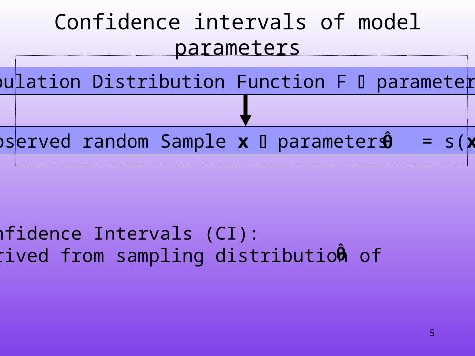
Confidence intervals of model parameters
Observed random Sample x parameters = s(x) θ̂
Population Distribution Function F parameters θ
Confidence Intervals (CI): derived from sampling distribution of θ̂

6
Bootstrap Confidence intervals
Observed random Sample x parameters = s(x) θ̂
Population Distribution Function F parameters θ
Empirical Distribution Function F̂
Bootstrap Sample x* parameters = s(x*) *θ̂
7
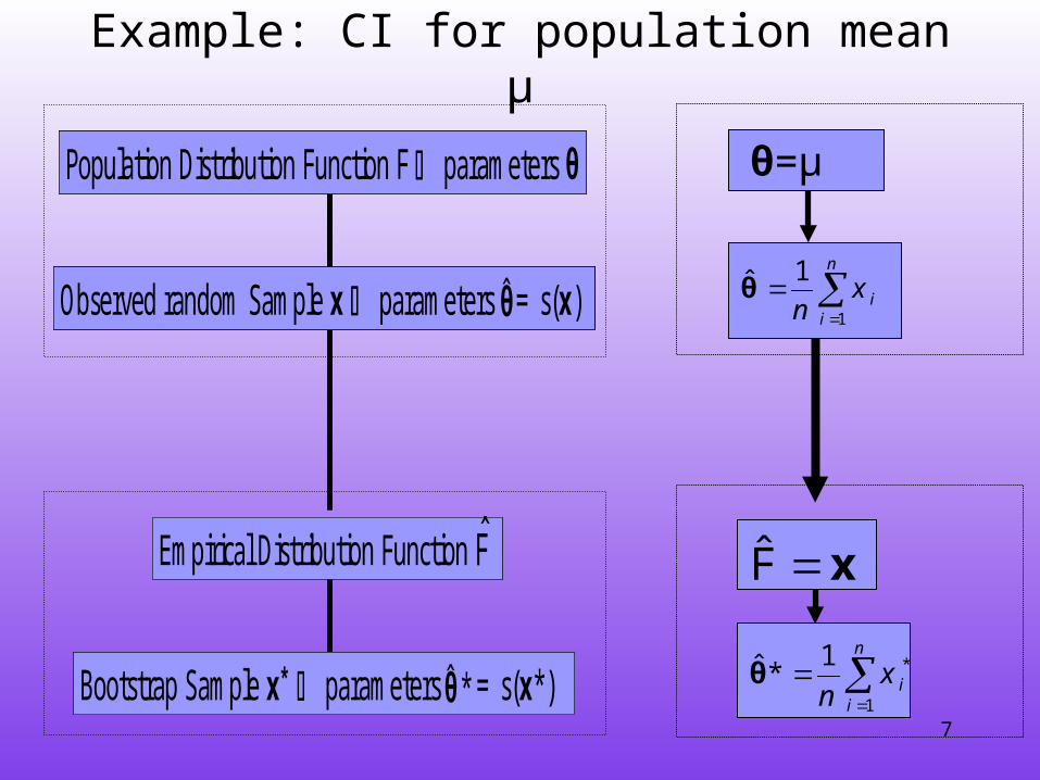
Example: CI for population mean μ
Observed random Sample x parameters = s(x) θ̂
Population Distribution Function F parameters θ
Empirical Distribution Function F̂
Bootstrap Sample x* parameters = s(x*) *θ̂
Observed random Sample x parameters = s(x) θ̂
Population Distribution Function F parameters θ
Observed random Sample x parameters = s(x) θ̂
Population Distribution Function F parameters θ
Observed random Sample x parameters = s(x) θ̂Observed random Sample x parameters = s(x) θ̂
Population Distribution Function F parameters θ
Empirical Distribution Function F̂
Bootstrap Sample x* parameters = s(x*) *θ̂
Empirical Distribution Function F̂
Bootstrap Sample x* parameters = s(x*) *θ̂
Empirical Distribution Function F̂Empirical Distribution Function F̂
Bootstrap Sample x* parameters = s(x*) *θ̂Bootstrap Sample x* parameters = s(x*) *θ̂
θ=μ
xF̂
n
iix
n 1
*1*θ̂
n
iix
n 1
1θ̂
8
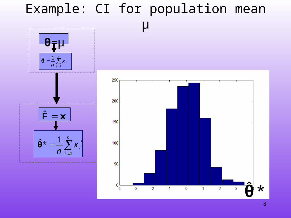
Example: CI for population mean μ
θ=μ
n
iix
n 1
1θ̂
xF̂
n
iix
n 1
*1*θ̂
*θ̂

9
Key questions for the Bootstrap procedure
1. Sample drawn from which Population(s)?
2. What is s(x) exactly?
3. If s(x) is non-unique, how to make s(x*) comparable?
4. How to define EDF?5. How to estimate CIs
from distribution of ?
Observed random Sample x parameters = s(x) θ̂
Population Distribution Function F parameters θ
Empirical Distribution Function F̂
Bootstrap Sample x* parameters = s(x*) *θ̂
Observed random Sample x parameters = s(x) θ̂
Population Distribution Function F parameters θ
Observed random Sample x parameters = s(x) θ̂
Population Distribution Function F parameters θ
Observed random Sample x parameters = s(x) θ̂Observed random Sample x parameters = s(x) θ̂
Population Distribution Function F parameters θ
Empirical Distribution Function F̂
Bootstrap Sample x* parameters = s(x*) *θ̂
Empirical Distribution Function F̂
Bootstrap Sample x* parameters = s(x*) *θ̂
Empirical Distribution Function F̂Empirical Distribution Function F̂
Bootstrap Sample x* parameters = s(x*) *θ̂Bootstrap Sample x* parameters = s(x*) *θ̂*θ̂

10
What’s next…
• Principal Component Analysis– Various answers to the key questions – Simulation study: What’s the quality
of the various resulting CIs?
• Real multi-way/block methods– Tucker3/PARAFAC– Multilevel Component Analysis – Principal Response Curve Model
11
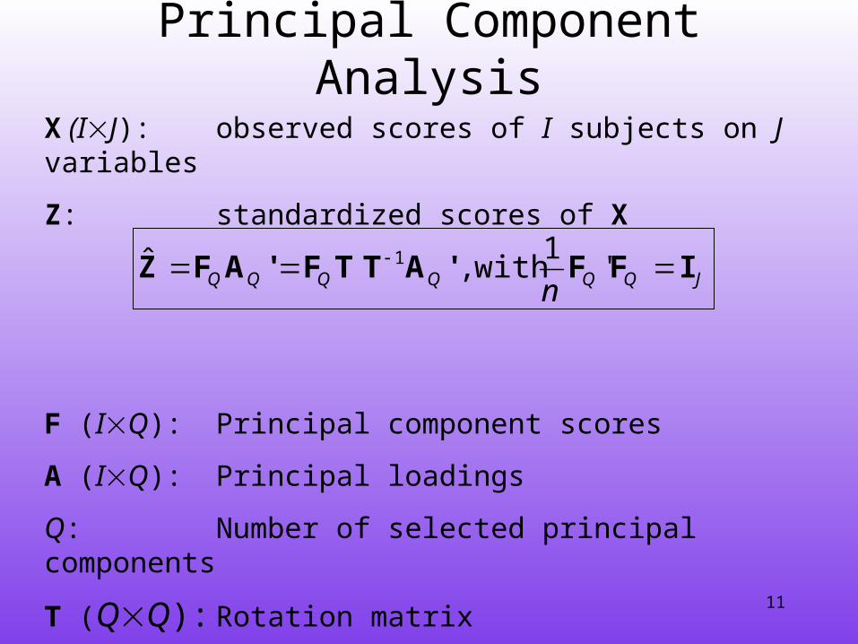
Principal Component Analysis
X (IJ): observed scores of I subjects on J variables
Z: standardized scores of X
F (IQ): Principal component scores
A (IQ): Principal loadings
Q: Number of selected principal components
T (QQ): Rotation matrix
JQQQQQQ nIFF'ATTF'AFZ '
1 with ,ˆ 1

12
1. Sample drawn from which Population(s)?
• ‘observed scores of I subjects on J variables’
13
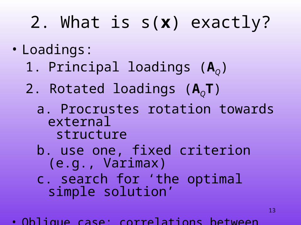
2. What is s(x) exactly?
• Loadings:1. Principal loadings (AQ)
2. Rotated loadings (AQT)
a. Procrustes rotation towards external structure
b. use one, fixed criterion (e.g., Varimax)
c. search for ‘the optimal simple solution’
• Oblique case: correlations between components
• Variance accounted for

14
3. If s(x) is non-unique, how to make s(x*)
comparable?• Loadings:
1. Principal loadings (AQ)
Sign of Principal loadings (AQ) is arbitrary:
reflect columns of AQ* to the same direction

15
1. Principal loadings (AQ)
Sign of Principal loadings (AQ) is arbitrary:
reflect columns of AQ* to the same direction
16
2. Rotated loadings (AQT)
a. Procrustes rotation towards external structure:
none (AQT* is unique)

17
2. Rotated loadings (AQT)
b. use one, fixed criterion (e.g., Varimax)
Sign & order of Varimax rotated loadings is arbitrary:
reflect & reorder columns of AQT*
18
2. Rotated loadings (AQT)c. search for ‘the optimal simple
solution’• How are bootstrap solutions AQT* found?
– For each bootstrap solution: look for ‘optimal simple loadings’ (unfeasible): reflect & reorder columns of AQT*
– Procrustes rotation towards ‘optimally simple’ sample loadings: none (AQT* is unique)

19
‘Fixed criterion’ versus ‘Procrustes towards (simple) sample
loadings’Instable varimax rotated solutions over
samples?Varimax rotated bootstrap solutions
Procrustes rotated bootstrap solutions

20
– non-parametric: Xb: rowwise resampling of Z
– semi-parametric:
),0(~ (e.g.) with ,ˆb NZX
– parametric:elements of Xb from particular p.d.f.
JQQQQQQ nIFF'ATTF'AFZ '
1 with ,ˆ 1
4. How to define the EDF?
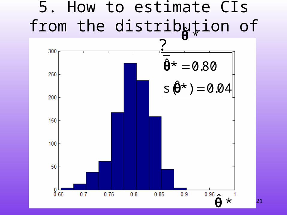
21*θ̂
040
800
.*)ˆs(
.*ˆ
θ
θ
5. How to estimate CIs from the distribution of ?*θ̂

22*θ̂
0.04*)θ̂s(se*
0.80*θ̂
• Based on bootstrap standard error (se*)–Wald ( )–...
)1(*seθ̂ z
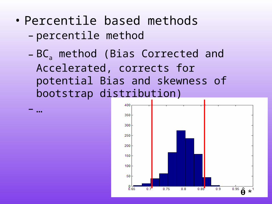
23*θ̂
• Percentile based methods
– BCa method (Bias Corrected and Accelerated, corrects for potential Bias and skewness of bootstrap distribution)
– …
– percentile method
24
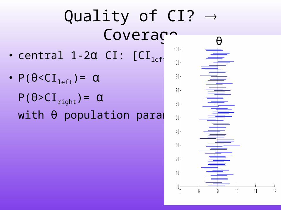
Quality of CI? Coverage
• central 1-2α CI: [CIleft;CIright)
• P(θ<CIleft)= α
P(θ>CIright)= α with θ population parameter
θ
25
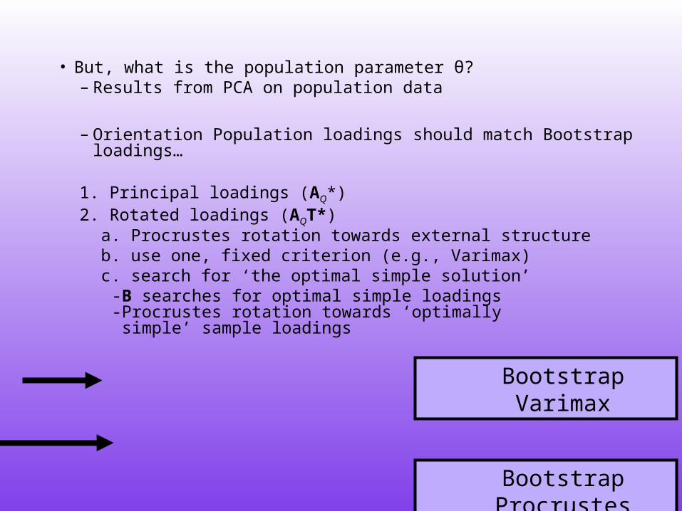
• But, what is the population parameter θ?– Results from PCA on population data
– Orientation Population loadings should match Bootstrap loadings…
1. Principal loadings (AQ*)2. Rotated loadings (AQT*)
a. Procrustes rotation towards external structureb. use one, fixed criterion (e.g., Varimax)c. search for ‘the optimal simple solution’
-B searches for optimal simple loadings-Procrustes rotation towards ‘optimally simple’ sample loadings
Bootstrap Varimax
Bootstrap Procrustes

26
Simulation study
• CI’s for Varimax rotated Sample loadings• Data properties varied:
– VAF in population (0.8,0.6,0.4)– number of variables (8, 16)– sample size (50, 100, 500)– distribution of component scores
(normal, leptokurtic, skew)– simplicity of loading matrix
(simple, halfsimple, complex)• Design completely crossed, 1000 replicates
per cell
27
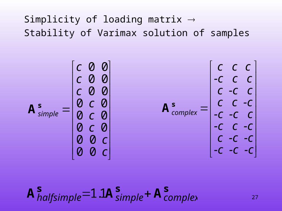
Simplicity of loading matrix Stability of Varimax solution of samples
c c
c c c
c c c
simple
0000
000000000000
sA
-c -c -c c -c -c-c c -c-c -c c c c -c c -c c-c c c
c c c
complex
sA
sss AAA complexsimplehalfsimple 1.1
28
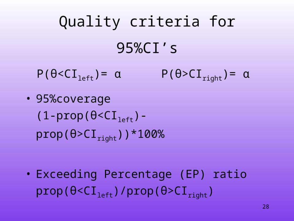
Quality criteria for 95%CI’s
P(θ<CIleft)= α P(θ>CIright)= α
• 95%coverage
(1-prop(θ<CIleft)-prop(θ>CIright))*100%
• Exceeding Percentage (EP) ratio
prop(θ<CIleft)/prop(θ>CIright)

29
30
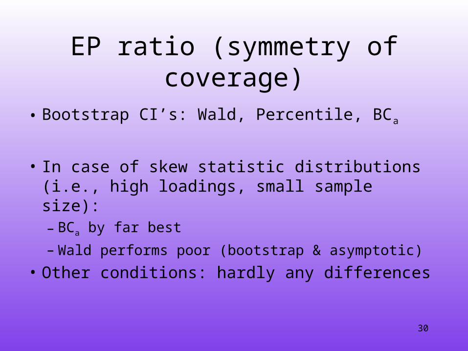
EP ratio (symmetry of coverage)
• Bootstrap CI’s: Wald, Percentile, BCa
• In case of skew statistic distributions (i.e., high loadings, small sample size):– BCa by far best
– Wald performs poor (bootstrap & asymptotic)
• Other conditions: hardly any differences
31
32
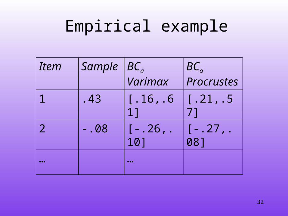
Empirical example
Item Sample
BCa
VarimaxBCa
Procrustes
1 .43 [.16,.61] [.21,.57]
2 -.08 [-.26,.10] [-.27,.08]
… …
33
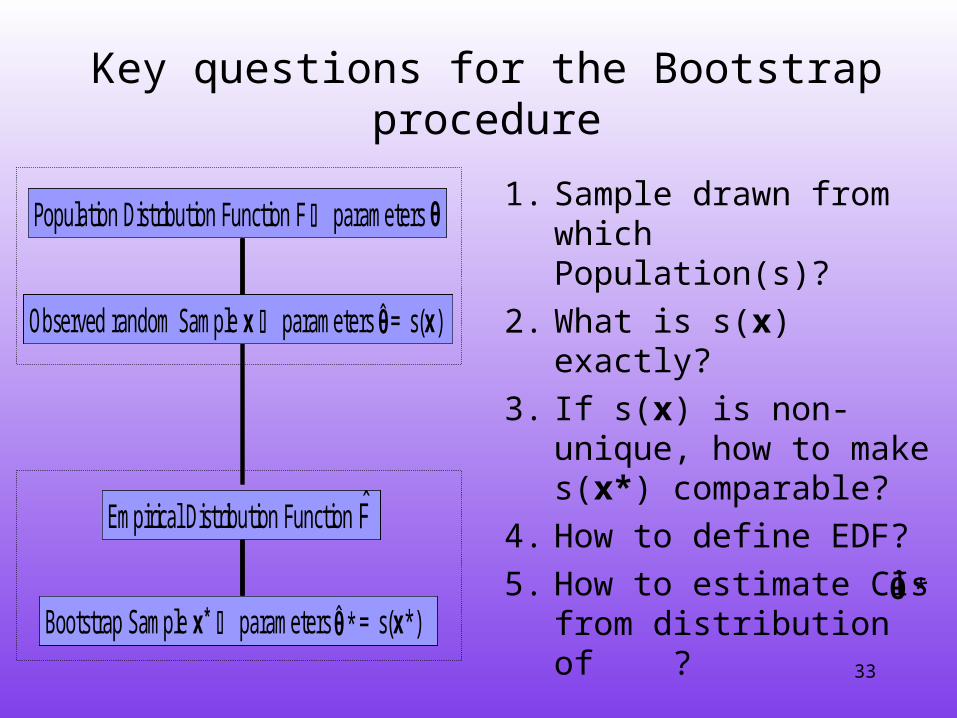
Key questions for the Bootstrap procedure
1. Sample drawn from which Population(s)?
2. What is s(x) exactly?
3. If s(x) is non-unique, how to make s(x*) comparable?
4. How to define EDF?5. How to estimate CIs
from distribution of ?
Observed random Sample x parameters = s(x) θ̂
Population Distribution Function F parameters θ
Empirical Distribution Function F̂
Bootstrap Sample x* parameters = s(x*) *θ̂
Observed random Sample x parameters = s(x) θ̂
Population Distribution Function F parameters θ
Observed random Sample x parameters = s(x) θ̂
Population Distribution Function F parameters θ
Observed random Sample x parameters = s(x) θ̂Observed random Sample x parameters = s(x) θ̂
Population Distribution Function F parameters θ
Empirical Distribution Function F̂
Bootstrap Sample x* parameters = s(x*) *θ̂
Empirical Distribution Function F̂
Bootstrap Sample x* parameters = s(x*) *θ̂
Empirical Distribution Function F̂Empirical Distribution Function F̂
Bootstrap Sample x* parameters = s(x*) *θ̂Bootstrap Sample x* parameters = s(x*) *θ̂*θ̂
34
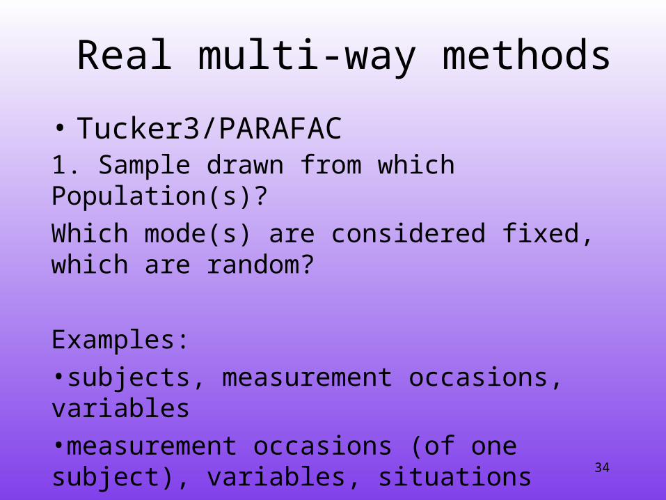
Real multi-way methods
• Tucker3/PARAFAC1. Sample drawn from which Population(s)?Which mode(s) are considered fixed, which are random?
Examples: •subjects, measurement occasions, variables•measurement occasions (of one subject), variables, situations•judges, food types, variables
35
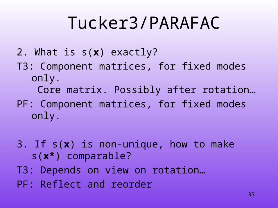
Tucker3/PARAFAC
2. What is s(x) exactly?T3: Component matrices, for fixed modes
only. Core matrix. Possibly after rotation…
PF: Component matrices, for fixed modes only.
3. If s(x) is non-unique, how to make s(x*) comparable?
T3: Depends on view on rotation…PF: Reflect and reorder
36
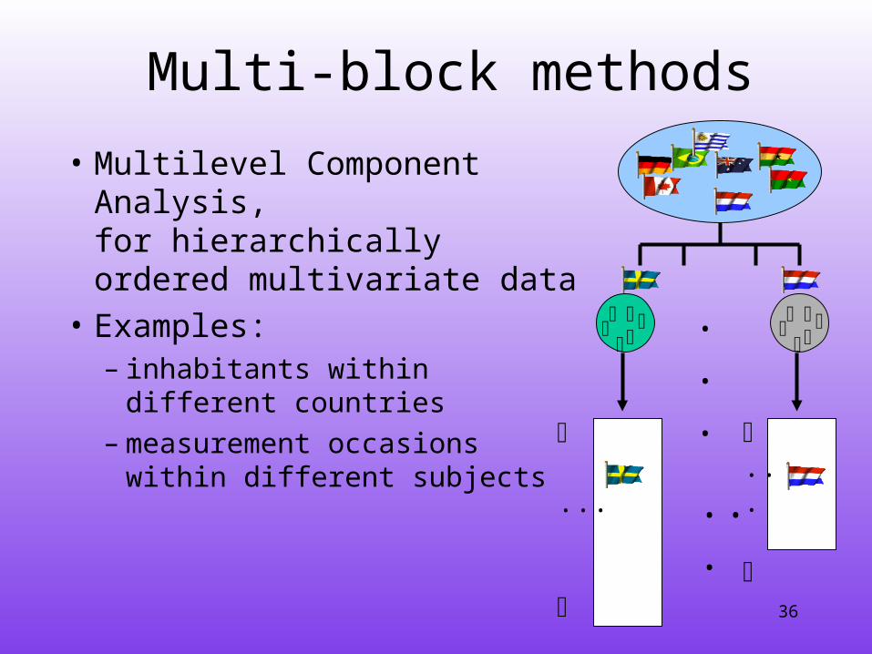
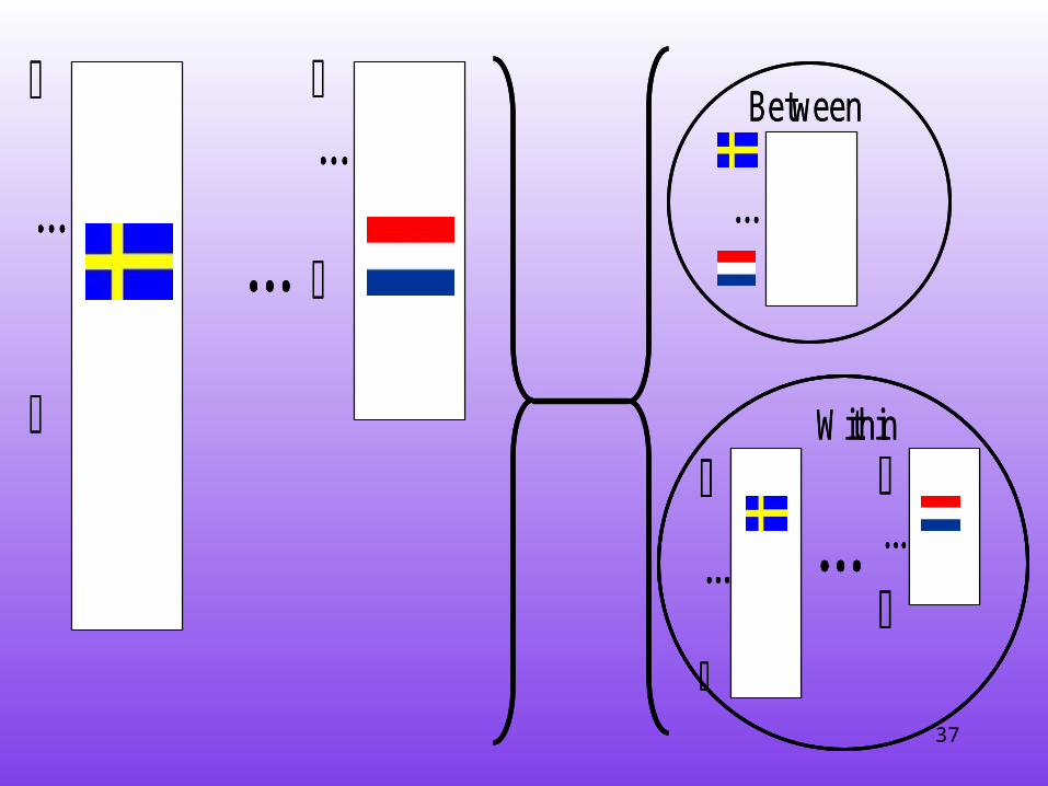
Multi-block methods
• Multilevel Component Analysis, for hierarchically ordered multivariate data
• Examples: – inhabitants within different
countries– measurement occasions
within different subjects
...
...
...
...
37
...
...
...
Between
...
Within
......
...
...
...
...
...
...
...
Between
...
Within
......
...
...
...
...
...
...
...
...
...
...

38
...
...
...
Between
...
Within
......
...
...
...
...
...
...
...
Between
...
Within
......
...
...
...
...
...
...
...
...
...
...
National character
Weighted PCA
(Dis)similarities between inhabitants within each countrySimultaneous
Component Analysis

39
1. Sample drawn from which population(s)?
Which mode(s) are considered fixed, which are random?
•inhabitants within different countries•measurement occasions within different subjects•pupils within classes

40
Another multi-block method
• Principal response curve model for longitudinal multivariate data, obtained from objects within experimental conditions
• ‘How is the development over time influenced by the experimental conditions?’

41
-5 0 5 10 15 20 25-0.4
-0.3
-0.2
-0.1
0
Can
onic
al c
oeff
icie
nt
Time
d=1
d=2d=3
d=4
first PRCs of Invertebrate data
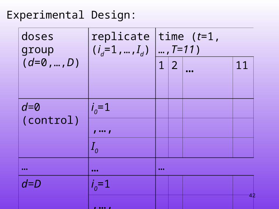
42
doses group (d=0,…,D)
replicate (id=1,…,Id)
time (t=1,…,T=11)
1 2 … 11
d=0 (control)
i0=1
,…,
I0
… … …
d=D i0=1
,…,
ID
Experimental Design:
43
• Results from a simulation experiment:– BCa confidence bands quality improves
• with decreasing replicate variation, and simpler error structures
• with increasing sample size• ...but even sample size of 20 replicates
per condition generally yields satisfactory results

44
To conclude
• How to estimate CIs in component analysis?– Use the bootstrap!– 5 Key questions for the Bootstrap procedure
• uniqueness of sample solution?• which modes are random/fixed?• ...
• And what is the quality?– Generally reasonable