Zhen Zeng Tucker Balch Manuela Veloso

Deep Video Prediction for Time Series ForecastingZhen Zeng

J. P. Morgan AI ResearchNew York, NY, USA

[email protected]

Tucker BalchJ. P. Morgan AI Research

New York, NY, [email protected]

Manuela VelosoJ. P. Morgan AI Research

New York, NY, [email protected]

ABSTRACTTime series forecasting is essential for decision making in manydomains. In this work, we address the challenge of predicting pricesevolution among multiple potentially interacting financial assets. Asolution to this problem has obvious importance for governments,banks, and investors. Statistical methods such as Auto RegressiveIntegrated Moving Average (ARIMA) are widely applied to theseproblems. In this paper, we propose to approach economic time se-ries forecasting of multiple financial assets in a novel way via videoprediction. Given past prices of multiple potentially interactingfinancial assets, we aim to predict the prices evolution in the future.Instead of treating the snapshot of prices at each time point as avector, we spatially layout these prices in 2D as an image similarto market change visualization, and we can harness the power ofCNNs in learning a latent representation for these financial assets.Thus, the history of these prices becomes a sequence of images, andour goal becomes predicting future images. We build on advancesfrom computer vision for video prediction. Our experiments involvethe prediction task of the price evolution of nine financial assetstraded in U.S. stock markets. The proposed method outperformsbaselines including ARIMA, Prophet and variations of the proposedmethod, demonstrating the benefits of harnessing the power ofCNNs in the problem of economic time series forecasting.

CCS CONCEPTS•Computingmethodologies→ Image representations; •Math-ematics of computing → Time series analysis.

KEYWORDStime-series forecasting, economic forecasting, image representa-tions, neural networks, ARIMA, visualizationsACM Reference Format:Zhen Zeng, Tucker Balch, and Manuela Veloso. 2021. Deep Video Predictionfor Time Series Forecasting. In 2nd ACM International Conference on AI inFinance (ICAIF’21), November 3–5, 2021, Virtual Event, USA. ACM, New York,NY, USA, 7 pages. https://doi.org/10.1145/3490354.3494404

1 INTRODUCTIONIn many time series forecasting tasks such as predictions on market,sales, and weather, the underlying data is non-image. Common

Permission to make digital or hard copies of all or part of this work for personal orclassroom use is granted without fee provided that copies are not made or distributedfor profit or commercial advantage and that copies bear this notice and the full citationon the first page. Copyrights for components of this work owned by others than ACMmust be honored. Abstracting with credit is permitted. To copy otherwise, or republish,to post on servers or to redistribute to lists, requires prior specific permission and/or afee. Request permissions from [email protected]’21, November 3–5, 2021, Virtual Event, USA© 2021 Association for Computing Machinery.ACM ISBN 978-1-4503-9148-1/21/11. . . $15.00https://doi.org/10.1145/3490354.3494404

time

time

Δprice

Non-image Time-Series Forecasting Video Prediction

Figure 1: We transform the problem of non-image time se-ries forecasting into the problem of video prediction. Forexample, given a task of forecasting the relative close pricechange of 9 different publicly traded assets in the future, ourapproach first transforms the numerical data at each timestamp into an image frame (e.g., a 3x3 tile heatmap), and pre-dicts future image frames via a video prediction technique.

statistical methods such as ARIMA have been widely adopted acrossthese domains for time series forecasting tasks. These methodsconsider the history of the numerical data and predict the futurevalues of the observed data. On the other hand, given tables orlists of numerical data, humans rely much more on visualizingthe underlying numerical data rather than directly eyeing at thenumbers themselves to develop a high-level understanding of thedata. For example, experienced traders develop intuition for makingbuy/sell decisions by observing visual market charts [2].

The power of visualizations lies in that they provide spatialstructural information [22] when laying out the underlying datain 2D images, which is not available in the original data. Whenlooking at 2D images, human eyes are proficient at capturing spatialstructure or patterns to help make better decisions or predictions.Advances in deep learning and computer vision have shown thatConvolutional Neural Networks (CNNs) [13] carry the capabilitiesto extract features of local spatial regions, which enables systemsto recognize spatial patterns such as those in object detection andrecognition tasks.

Inspired by how humans benefit from 2D visualizations of nu-merical data, we propose to spatially layout numerical informationin 2D images similarly to market change visualizations. Then wetake the advantage of CNNs for time series forecasting tasks, whichwere originally studied in non-image domains. In this paper, wetake a unique perspective in predicting non-image time-series datathrough the lens of computer vision. To achieve this, we proposeto first visualize the multivariate time-series data as a sequence

arX

iv:2

102.

1206

1v2

[cs

.CV

] 3

Nov

202

1

ICAIF’21, November 3–5, 2021, Virtual Event, USA Zeng Z., et al.

Non-image Time-SeriesData History

InputVideo Frames

Video Prediction Neural Network

map input output

PredictedVideo Frames

map

PredictedNon-image Data

time

time

Δprice

time

Δprice

Figure 2: Method overview. First, we turn non-image time-series data history into a video frame at each time stamp. Then, weuse a video prediction neural network to predict future video frames. Finally, we map the predicted video frames back to thenumerical data space.

of images, thus forming a video, and then build on video predic-tion techniques [1, 7] to predict future image frames, i.e., futurevisualizations of the underlying non-image data.

Our experiments focus on the task of forecasting market changesover time, where 9 publicly traded assets including 2 stocks and 7Exchange-Traded Funds (ETFs) are being considered as shown inFigure 1. We demonstrate that our proposed method outperformsother baselines, such as DeepInsight [22], ARIMA and Prophet (onnon-image numerical data), as well as variations of our proposedmethod. Our study shows that our method is able to learn high-level knowledge jointly over multiple assets, and produces betterprediction accuracy compared to either learning each asset inde-pendently, or learning multiple assets as a vector other than a 2Dimage.

2 RELATEDWORKTime series forecasting [11] has many applications across diversedomains, e.g. finance, climate, resource allocation, etc. Among a col-lection of statistical tools, exponential smoothing and ARIMAare two of the most widely adopted approaches for time seriesforecasting. Exponential smoothing predicts the future value of arandom variable by a weighted average of its past values, where theweight associated with each past value decreases exponentially aswe go back in time. Several variations of exponential smoothing areproposed to consider trend [8] and seasonality [9, 24] in the data.ARIMA combines autoregressive and moving average models forforecasting and ARIMAs use differencing to help reduce trend andseasonality in the data. However, ARIMA, as well as VAR (vectorautoregressive) model for multivariate cases, cannot capture nonlin-ear patterns in time series, rendering it insufficient for forecastingwhen nonlinear patterns occur. Our experiments show that a neuralnetwork based approach, which is nonlinear, outperforms ARIMA.

Recent works [17, 20, 26] focus on combinations of statisticaland machine learning methods to improve forecasting accuracy.Yet the data involved in these time series forecasting tasks [15] isusually non-image.

In this work, we provide a new perspective of the time seriesforecasting problem, by transforming it into a video predictionproblem. We visualize the underlying numerical data as an image ateach time stamp, and bring recent advances in video prediction [16]from the field of computer vision for forecasting.

Early works on video prediction directly predict future appear-ance as a composition of predicted image patches [18], withoutexplicit modeling of temporal dynamics in the video. Others haveattempted to learn explicit transformations (ae.g. per pixel mo-tion [19], or affine transformations [6]) that synthesize the futureframe from the last observed frame. These works learn to inferthe transformation parameters from observed video frames. Morerecently, researchers aim to disentangle motion and visual con-tent [7, 10] in videos. The prediction task becomes more tractablebecause prediction can be performed in a latent space modeling thetemporal dynamics. Thus, we built on [7] for video prediction.

Similar to our work, there are recent works that also tackle clas-sification or regression tasks on non-image data from the computervision perspective. [2, 4] developed image classifiers for stock anal-ysis, e.g. buy/sell, and positive/negative price change. [22] proposedDeepInsight which visualizes non-image data as an image throughdimension reduction technique, and trained CNNs for classifica-tion on cancer types given visualized gene expressions. AlthoughDeepInsight achieves promising classification accuracy as discussedin [22], our experiment suggests that DeepInsight is not necessarilysuitable for prediction tasks. [14] proposed to transform non-imagedata into recurrence images, and then use CNNs to extract imagefeatures to predict weights for averaging multiple statistical fore-casting methods. However, their method is concerned only withunivariate time series forecasting. Real-world problems often in-volve multivariate time series forecasting, and it’s important tounderstand the relationships between multiple variables. Our workaddresses multivariate time series forecasting as discussed in theexperiments.

3 METHODSGiven a time series of a random variable {x0, x1, · · · , x𝑡 }, wherex𝑡 ∈ R𝑑 , the goal is to predict the values of the random variable atfuture time stamps {x𝑡+1, x𝑡+2 . · · · }. In this work, for each time 𝑡 , wevisualize x𝑡 as an image, i.e., x𝑡 ↦→ I𝑡 . Then the task of predictingx𝑡+Δ𝑡 is converted to a video prediction task, i.e., predicting futureimage frames I𝑡+Δ𝑡 given an input video clip. We will explain howwe spatially layout data in 2D and the video prediction method asfollowing.

Deep Video Prediction for Time Series Forecasting ICAIF’21, November 3–5, 2021, Virtual Event, USA

Figure 3: Video prediction network. Variational autoencoders are learned for encoding and decoding the input and outputvideo frames. LSTM learns the temporal features of underlying dynamics. Figure recreated from [7].

3.1 VisualizationThe particular visualizations of the underlying data varies acrossdomains. Humans usually rely on domain knowledge to developvisualizations of numerical data, and these visualizations evolveover time as humans continuously improve them. We do not aimto provide an unified way to visualize all numerical data acrossarbitrary domains. We believe domain knowledge is important (aswe will also show in experiments), and aiming to provide an unifiedway of visualizations poses the risk of throwing away domainknowledge.

Regardless of domains, the rule of thumb for generating visual-izations of time-series data is that correlated data shall be visualizedin a way such that they are spatially close to each other in the 2Dimage. The intuitive reason for this principle is that when lookingat visualizations, CNN is good at extracting structural features inlocal regions represented by its limited receptive field. By visualiz-ing correlated data (i.e. potentially dependent) spatially close in animage, CNN gets the chance to learn the high-level joint features ofthese correlated data, which can be exploited for prediction tasks.As we later show in our experiments, separating correlated data invisualizations results in a drop of prediction accuracy.

Here we discuss the particular visualization that we use for themarket change prediction task in our experiments. Given the time-series market history of 9 assets in terms of relative percentagechange 𝛿 of close values, i.e., x𝑡 = [𝛿1𝑡 , · · · , 𝛿9𝑡 ]𝑇 , the goal is topredict future percentage changes of these assets. Following thesame intuition of a commonly adopted market change visualizationin industry from Finviz1, we visualize the percentage changes ofthese 9 assets in a 3x3 tile heatmap, as shown in Figure 1. Wewill discuss how domain knowledge helps arrange these 9 assetsand achieve better performance in experiments and discussion. To

1https://finviz.com/map.ashx?t=sec_all

visualize numerical data into pixels, we convert the percentagechange of 𝑖th asset at time 𝑡 , 𝛿𝑖𝑡 , into a pixel 𝑝 ∈ I𝑡 ,

𝑝 = 𝑆 (𝛿𝑖𝑡 ) ∗ 255 (1)

𝑆 (𝑥) = 11 + 𝑒−𝑥

(2)

where 𝑆 : R ↦→ [0, 1] is a sigmoid function, thus 𝑝 ∈ [0, 255]. Forexample, if 𝛿𝑖𝑡 = 3, meaning that 𝑖th asset has a 3% increase in itsclose value at time 𝑡 , then the corresponding pixel value will be243. As such, the higher the percentage increase, the brighter thevisualized pixel. And the more the percentage decrease, the darkerthe visualized pixel.

3.2 Video PredictionIn this work, we adapted a video prediction network SRVP (Sto-chastic Latent Residual Video Prediction) [7] in computer visionfor the economic time series forecasting task. Compared to mostworks in the literature which rely on image-autoregressive recur-rent networks, SRVP decouples frame synthesis and video dynamicsestimation. SRVP has shown to outperform prior state-of-the-artmethods across a simulated [3] dataset, and real-world datasets ofhuman activities [12, 21] as well as robot actions [5]. We adaptedthe video prediction network from predicting frames in naturalvideo to predicting frames in visualizations.

As shown in Figure 3, SRVP explicitly models the hidden state𝑦𝑡 as well as the dynamics (the residual gets added to 𝑦𝑡 from 𝑓\at each time point) of the video in a latent space. Specifically, 𝑥𝑡denotes the input frame at time 𝑡 , 𝑦𝑡 is the latent state variable, 𝑧𝑡is the latent state dynamics variable, and 𝑤 is a content variablethat encodes the static content in the video (e.g. static background,constant shape of foreground object, etc).

ICAIF’21, November 3–5, 2021, Virtual Event, USA Zeng Z., et al.

DAL TSLA USO

SPY DIA TLT

VNQ GLD AGG

SPY VNQ USO

TSLA AGG TLT

DAL GLD DIA

DAL

1

2 345 6

7

Video-Full Video-Ind Video-Shuffled Video-DeepInsight

Figure 4: Visualization examples used in different methods. Video-Full: correlated assets are placed close to each other in thesame image; Video-Ind: each asset is visualized independently in separate images; Video-Shuffled: correlated assets are placedapart from each other in the same image; Video-DeepInsight: assets visualized using method proposed in [22], where eachasset corresponds to a single pixel on the image, resulting in sparse points in the image. Specifically, 1 is USO, 2 is GLD, 3 isTLT, 4 is AGG, region 5 includes SPY, DIA, VNQ, 6 is DAL, 7 is TSLA (dark pixel). Note that DIA and VNQ gets placed at the samepixel location based on the proposed method in [22]. As a result, we can only visualize one of the two assets and overwrite theother one, which prevents the network from learning the overwritten asset (VNQ is overwritten in our experiments).

For each input frame 𝑥𝑡 , ℎ𝜙 is an CNN-based encoder that en-codes 𝑥𝑡 into encoded frame 𝑥𝑡 . Given encoded frames 𝑥1:𝑘 of theinput video, the initial latent state 𝑦1 ∼ N(`𝑦

𝜙, 𝜎

𝑦

𝜙) is obtained

through variational inference. We use 𝑘 = 5 across our experiments.The latent state 𝑦𝑡 then propagates forward with a transition func-tion 𝑓\ ,

𝑦𝑡+1 = 𝑦𝑡 + 𝑓\ (𝑧𝑡+1)where 𝑓\ is an Multilayer Perception (MLP) that learns the first-order movement of latent state 𝑦𝑡 . As part of the input to 𝑓\ , thelatent dynamics 𝑧𝑡 ∼ N(`𝑧

𝜙, 𝜎𝑧

𝜙) is inferred through an LSTM on the

encoded input frames. The content variable𝑤 is inferred througha permutation-invariant function [25] given few encoded frames.Lastly, 𝑔\ is a decoder network that concatenates the content vari-able𝑤 and latent state 𝑦𝑡 and decode it back to the original spaceof 𝑥𝑡 , thus producing the estimated 𝑥𝑡 . Note that at testing time,we need to predict future 𝑧𝑡 when 𝑥𝑡 is not available. Instead ofinferring 𝑧𝑡 through LSTM on 𝑥𝑡 s as explained earlier, 𝑧𝑡 is inferredfrom 𝑦𝑡−1 through two MLPs to generate `\ , 𝜎\ , which are trainedto fit 𝑧𝑡+1 ∼ N(`\ (𝑦𝑡 ), 𝜎\ (𝑦𝑡 )𝐼 ).

In our experiments, we used VGG16 [23] as the encoder networkℎ𝜙 and decoder network 𝑔\ (mirrored VGG16). The image size is64x64, and we choose to keep this generic choice so that we don’ttailor it towards the specific task in our experiments. We used 50dimensions for both 𝑦𝑡 and 𝑧𝑡 . The loss function is negative log-likelihood and we used L2 regularization to prevent overfitting. Weused Adam for optimization during training, with learning rate𝛼 = 3e−3, and 𝛽1 = 0.9, 𝛽2 = 0.999, 𝜖 = 1e−8.

4 EXPERIMENTSThe experiments were conducted on a Linux machine with In-tel(R) Xeon(R) Platinum 8259CL CPU @ 2.50GHz, 19 GB RAM, andNVIDIA T4 GPU. Our experiments focus on the task of forecastingmarket changes. We consider 9 assets in the market:

• DAL (Delta Air Lines, Inc)

• SPY (SPDR S&P 500 ETF Trust)• VNQ (Vanguard Real Estate Index Fund ETF Shares)• TSLA (Tesla, Inc.)• DIA (SPDR Dow Jones Industrial Average ETF Trust)• GLD (SPDR Gold Shares)• USO (United States Oil Fund, LP)• TLT (iShares 20+ Year Treasury Bond ETF)• AGG (iShares Core U.S. Aggregate Bond ETF)

We deliberately selected a diverse group of assets. There existsinterdependencies between these assets. For instance, the airlinestock DAL will usually go up in price when the oil ETF USO goesdown in price. This is because fuel derived from oil is one of theprimary operating costs for airlines, and a decrease in fuel pricescan be predictive of future profits. Similarly, SPY which representslarge U.S. company stocks is typically inversely related to the move-ment of TLT which represents long term bonds. Other assets inthe mix share other correlations or anti-correlations that reflect thestructure of the U.S. economy. We show that our method is ableto learn and exploit these hidden interdependencies to make jointpredictions.

In our experiments, we used the closing prices of these assetsfrom June 29th, 2010 to Dec 31rd, 2019 (source: Yahoo!-Finance2).We pre-processed the collected data by calculating the percentagechange of each asset’s closing price on each day with respect toits closing price 5 days ago. The task is that given the percentagechanges of assets over 5 consecutive days, we need to predict thefuture percentage changes of assets for the next 10 days. We splitthe historical data from June 29th, 2010 to Dec 31rd, 2018 for train-ing and validation (we did 95% split for training and validation),and Jan 1st, 2019 to Dec 31rd, 2019 for testing. We benchmarkedthe prediction performance of our proposed video prediction basemethod (referred as Video-Full below), against baseline methods

2https://finance.yahoo.com/

Deep Video Prediction for Time Series Forecasting ICAIF’21, November 3–5, 2021, Virtual Event, USA

0.0

0.2

0.4

0.6

0.8

DAL SPY VNQ TSLA DIA GLD USO TLT AGG

Video-Full Video-Ind Video-Shuffled Video-DeepInsight VectorARIMA Prophet

Figure 5: Prediction accuracy of proposed method againstbaselines with _ = 0.5 in evaluation metric (Eq. 4).

including ARIMA and Prophet on original non-image data, as wellas variations of the proposed method. Specifically,

• Video-Full: We turn the numerical data of market percent-age change into visualizations of 3x3 tile heatmap as ex-plained in section 3.1. Then 5 frames are given as input tothe SRVP neural network, which outputs predicted 10 futureframes. Thus, the learned SRVP neural network predicts all 9assets market change jointly. Note that the 3x3 tile arrange-ments of the 9 assets are based on domain knowledge, suchthat known to be correlated assets are placed close to eachother.

• Video-Ind: Instead of visualizing all 9 assets in a 3x3 tileheatmap and learn to predict jointly as in Video-Full, here weturn each asset market percentage change into a single tileheatmap, thus producing one video clip for each asset. Foreach asset, we independently train a SRVP neural networkto predict its future percentage change.

• Video-Shuffled: This baseline method is the same as Video-Full, except that 3x3 tile arrangements of the 9 assets areshuffled such that it goes against the domain knowledge,meaning that known to be correlated assets are placed apartfrom each other.

• Video-DeepInsight: As discussed in section 2, DeepInsight[22] takes a similar perspective of converting non-image datato image data, and adopt computer vision techniques on theimage data. Here we use their proposed method to visualizethe non-image data, by corresponding each dimension ofthe non-image data with a 2D pixel coordinate on the imageplane through PCA. We then apply SRVP on the resultingvisualizations.

• Vector: Instead of turning numerical data into 2D heatmapsas in the proposed method, here we directly use the originalnumerical data (normalized to [0, 1]) as a 9x1 vector. In or-der to use the same SRVP network architecture as in otherbaselines for fair comparison, we repeat the 9x1 vectors tomatch the same size of input used in other baselines. Notethat this method can be perceived as a neural network basednonlinear vector autoregressive model.

0.0

0.2

0.4

0.6

0.8

DAL SPY VNQ TSLA DIA GLD USO TLT AGG

Video-Full Video-Ind Video-Shuffled Video-DeepInsight VectorARIMA Prophet

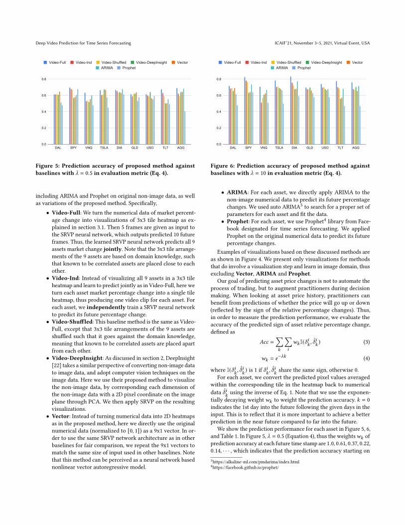
Figure 6: Prediction accuracy of proposed method againstbaselines with _ = 10 in evaluation metric (Eq. 4).

• ARIMA: For each asset, we directly apply ARIMA to thenon-image numerical data to predict its future percentagechanges. We used auto ARIMA3 to search for a proper set ofparameters for each asset and fit the data.

• Prophet: For each asset, we use Prophet4 library from Face-book designated for time series forecasting. We appliedProphet on the original numerical data to predict its futurepercentage changes.

Examples of visualizations based on these discussed methods areas shown in Figure 4. We present only visualizations for methodsthat do involve a visualization step and learn in image domain, thusexcluding Vector, ARIMA and Prophet.

Our goal of predicting asset price changes is not to automate theprocess of trading, but to augment practitioners during decisionmaking. When looking at asset price history, practitioners canbenefit from predictions of whether the price will go up or down(reflected by the sign of the relative percentage changes). Thus,in order to measure the prediction performance, we evaluate theaccuracy of the predicted sign of asset relative percentage change,defined as

𝐴𝑐𝑐 =∑︁𝑘

∑︁𝑖

𝑤𝑘 I(𝛿𝑖𝑘 , 𝛿𝑖𝑘) (3)

𝑤𝑘 = 𝑒−_𝑘 (4)

where I(𝛿𝑖𝑘, 𝛿𝑖

𝑘) is 1 if 𝛿𝑖

𝑘, 𝛿𝑖

𝑘share the same sign, otherwise 0.

For each asset, we convert the predicted pixel values averagedwithin the corresponding tile in the heatmap back to numericaldata 𝛿𝑖

𝑘using the inverse of Eq. 1. Note that we use the exponen-

tially decaying weight𝑤𝑘 to weight the prediction accuracy. 𝑘 = 0indicates the 1st day into the future following the given days in theinput. This is to reflect that it is more important to achieve a betterprediction in the near future compared to far into the future.

We show the prediction performance for each asset in Figure 5, 6,and Table 1. In Figure 5, _ = 0.5 (Equation 4), thus the weights𝑤𝑘 ofprediction accuracy at each future time stamp are 1.0, 0.61, 0.37, 0.22,0.14, · · · , which indicates that the prediction accuracy starting on3https://alkaline-ml.com/pmdarima/index.html4https://facebook.github.io/prophet/

ICAIF’21, November 3–5, 2021, Virtual Event, USA Zeng Z., et al.

Video-Full Video-Ind Video-Shuffled Video-DeepInsight Vector ARIMA Prophet_ = 0.5 0.65 ± 0.03 0.61 ± 0.04 0.61 ± 0.04 0.60 ± 0.06 0.61 ± 0.05 0.59 ± 0.06 0.53 ± 0.09_ = 10 0.76 ± 0.05 0.69 ± 0.08 0.69 ± 0.05 0.66 ± 0.05 0.65 ± 0.04 0.65 ± 0.04 0.54 ± 0.06

Table 1: Benchmark of prediction accuracy averaged over all assets in experiments.

the 5th day into the future do not matter as much. In Figure 6,_ = 10 (Equation 4), thus the weights𝑤𝑘 of prediction accuracy ateach future time stamp are 1.0, 0.0, · · · , indicating that we focus onthe prediction performance for the very next future day. Table 1summarizes the prediction accuracy averaged over all 9 assets foreach method.

As we can see, for either _ value, Video-Full outperforms otherbaseline methods across all 9 assets. More importantly, we showthat when learning to predict themarket changes jointly, we achievebetter prediction performance in Video-Full compared to Video-Ind, which learns to predict the change of each asset independently.This is because Video-Full allows the network to learn and exploitthe joint dynamics of these assets, where the interdependenciesbetween these assets play an important role.

We also show thatVideo-Full outperformsVideo-DeepInsight[22]. DeepInsight was originally proposed for classification tasks,and it corresponds each asset to a single pixel during visualization,resulting in a sparse set of points in the image (as shown in Figure4). A key issue is that this method can lead to different assets beingvisualized at the same pixel locations, thus pixel location conflicts,and one has to retain one of the assets information and discardthe others at such conflicted pixel locations. Although [22] showedDeepInsight to be suitable for classification tasks, we have shownthat it is not necessarily suitable for prediction tasks, due to thesparse visualization and especially pixel location conflicts. We willdiscuss the comparison between Video-Full and Video-Shuffledin detail in the later section 5.

Without the 2D structural information from visualized images,we can see that Vector, ARIMA and Prophet lead to less predic-tion accuracy than Video-Full in general. This suggests that byturning non-image time-series forecasting into a video predictionproblem, we have introduced informative 2D spatial structure in thevisualized images, which can be leveraged by CNNs in Video-Fullfor forecasting.

5 DISCUSSIONWhen comparing Video-Shuffled against Video-Full, we canclearly see a drop in prediction performance in Video-Shuffled.This is because Video-Shuffled suffers from the poor 3x3 tile ar-rangements of those 9 assets, where correlated assets are placedapart from each other in the visualization. On the contrary, Video-Full uses domain knowledge in finance to guide the 3x3 tile ar-rangements of those 9 assets. For instance, we place SPY and DIA,which represent the similar S&P 500 stock index and the Dow JonesIndustrial index respectively, next to one another. TLT and AGG,which represent large bond indexes are also placed adjacently.

Taking the advantage of domain knowledge, Video-Full placescorrelated assets close to each other during visualization, and achievesa better prediction performance because CNNs are able to extracthigh-level structural feature from local regions. As we scale up,

one interesting future direction is to learn to spatially layout mul-tivariate non-image data in 2D, with inductive bias from domainknowledge if available.

Although during the experimented period (2010-2019) the overallmarket goes up as the long-term trend, for the short-term day-to-day price of each asset, the price is not always going up. In particular,across our test dataset, the percentage of time when price goes upis [0.54, 0.70, 0.62, 0.56, 0.63, 0.61, 0.61, 0.55, 0.62], correspondingrespectively to assets DAL, SPY, VNQ, TSLA, DIA, GLD, USO, TLT,AGG. That means, if we take a naive predictor that always predictsthe prices to go up for the next day for all assets, then the predictionaccuracy will be [0.54, 0.70, 0.62, 0.56, 0.63, 0.61, 0.61, 0.55, 0.62].As shown in Figure 6, the prediction accuracy is [0.72, 0.83, 0.71,0.78, 0.83, 0.70, 0.74, 0.78, 0.76], which does provide a significantpercentage improvement of [0.33, 0.19, 0.15, 0.39, 0.32, 0.15, 0.21,0.42, 0.22] over the naive predictor for each asset respectively.

6 CONCLUSIONIn this paper, we demonstrate the benefit of learning to predict mul-tivariate non-image time-series data in the 2D image domain. Byspatially laying out original non-image data in 2D images, we con-vert the problem of time series forecasting into a video predictionproblem. We then adapt recent state-of-the-art video predictiontechnique from computer vision to the domain of economic timeseries forecasting. In our experiments, we show that the proposedmethod is able to learn spatial structural information from the vi-sualizations and outperforms other baseline methods in predictingfuture market changes. We provide a proof of concept that, by spa-tially laying out non-image data in 2D, we can harness the powerof CNNs and the proposed method outperforms other methods thateither treat each dimension of the multivariate data independently,or treat the multivariate data as a vector. This motivates an inter-esting future direction of learning to spatially layout non-imagedata in 2D for multivariate time-series forecasting problems.

Disclaimer: This paper was prepared for information purposesby the Artificial Intelligence Research group of J. P. Morgan Chase& Co. and its affiliates (“J. P. Morgan”), and is not a product ofthe Research Department of J. P. Morgan. J. P. Morgan makes norepresentation and warranty whatsoever and disclaims all liability,for the completeness, accuracy or reliability of the informationcontained herein. This document is not intended as investmentresearch or investment advice, or a recommendation, offer or solici-tation for the purchase or sale of any security, financial instrument,financial product or service, or to be used in any way for evalu-ating the merits of participating in any transaction, and shall notconstitute a solicitation under any jurisdiction or to any person, ifsuch solicitation under such jurisdiction or to such person wouldbe unlawful.

Deep Video Prediction for Time Series Forecasting ICAIF’21, November 3–5, 2021, Virtual Event, USA

REFERENCES[1] Mohammad Babaeizadeh, Chelsea Finn, Dumitru Erhan, Roy H Campbell, and

Sergey Levine. 2017. Stochastic variational video prediction. arXiv preprintarXiv:1710.11252 (2017).

[2] Naftali Cohen, Tucker Balch, and Manuela Veloso. 2020. Trading via imageclassification. In Proceedings of the First ACM International Conference on AI inFinance. 1–6.

[3] Emily Denton and Rob Fergus. 2018. Stochastic video generation with a learnedprior. arXiv preprint arXiv:1802.07687 (2018).

[4] Bairui Du and Paolo Barucca. 2020. Image Processing Tools for Financial TimeSeries Classification. arXiv preprint arXiv:2008.06042 (2020).

[5] Frederik Ebert, Chelsea Finn, Alex X Lee, and Sergey Levine. 2017. Self-supervisedvisual planning with temporal skip connections. arXiv preprint arXiv:1710.05268(2017).

[6] Chelsea Finn, Ian Goodfellow, and Sergey Levine. 2016. Unsupervised learning forphysical interaction through video prediction. In Advances in neural informationprocessing systems. 64–72.

[7] Jean-Yves Franceschi, Edouard Delasalles, Mickaël Chen, Sylvain Lamprier, andPatrick Gallinari. 2020. Stochastic Latent Residual Video Prediction. arXivpreprint arXiv:2002.09219 (2020).

[8] Everette S Gardner Jr and ED McKenzie. 1985. Forecasting trends in time series.Management Science 31, 10 (1985), 1237–1246.

[9] Charles C Holt. 2004. Forecasting seasonals and trends by exponentially weightedmoving averages. International journal of forecasting 20, 1 (2004), 5–10.

[10] Jun-Ting Hsieh, Bingbin Liu, De-An Huang, Li F Fei-Fei, and Juan Carlos Niebles.2018. Learning to decompose and disentangle representations for video prediction.In Advances in Neural Information Processing Systems. 517–526.

[11] Rob J Hyndman and George Athanasopoulos. 2018. Forecasting: principles andpractice. OTexts.

[12] Catalin Ionescu, Dragos Papava, Vlad Olaru, and Cristian Sminchisescu. 2013.Human3. 6m: Large scale datasets and predictive methods for 3d human sensingin natural environments. IEEE transactions on pattern analysis and machineintelligence 36, 7 (2013), 1325–1339.

[13] Alex Krizhevsky, Ilya Sutskever, and Geoffrey E Hinton. 2012. ImageNet Classifi-cation with Deep Convolutional Neural Networks. In Advances in Neural Infor-mation Processing Systems 25, F. Pereira, C. J. C. Burges, L. Bottou, and K. Q. Wein-berger (Eds.). Curran Associates, Inc., 1097–1105. http://papers.nips.cc/paper/

4824-imagenet-classification-with-deep-convolutional-neural-networks.pdf[14] Xixi Li, Yanfei Kang, and Feng Li. 2020. Forecasting with time series imaging.

Expert Systems with Applications 160 (2020), 113680.[15] Spyros Makridakis, Evangelos Spiliotis, and Vassilios Assimakopoulos. 2018. The

M4 Competition: Results, findings, conclusion and way forward. InternationalJournal of Forecasting 34, 4 (2018), 802–808.

[16] Sergiu Oprea, Pablo Martinez-Gonzalez, Alberto Garcia-Garcia, John AlejandroCastro-Vargas, Sergio Orts-Escolano, Jose Garcia-Rodriguez, and Antonis Argy-ros. 2020. A Review on Deep Learning Techniques for Video Prediction. arXivpreprint arXiv:2004.05214 (2020).

[17] Ping-Feng Pai and Chih-Sheng Lin. 2005. A hybrid ARIMA and support vectormachines model in stock price forecasting. Omega 33, 6 (2005), 497–505.

[18] MarcAurelio Ranzato, Arthur Szlam, Joan Bruna, Michael Mathieu, Ronan Col-lobert, and Sumit Chopra. 2014. Video (language) modeling: a baseline forgenerative models of natural videos. arXiv preprint arXiv:1412.6604 (2014).

[19] Fitsum A Reda, Guilin Liu, Kevin J Shih, Robert Kirby, Jon Barker, David Tarjan,AndrewTao, and BryanCatanzaro. 2018. Sdc-net: Video prediction using spatially-displaced convolution. In Proceedings of the European Conference on ComputerVision (ECCV). 718–733.

[20] Ali Safari and Maryam Davallou. 2018. Oil price forecasting using a hybrid model.Energy 148 (2018), 49–58.

[21] Christian Schuldt, Ivan Laptev, and Barbara Caputo. 2004. Recognizing humanactions: a local SVM approach. In Proceedings of the 17th International Conferenceon Pattern Recognition, 2004. ICPR 2004., Vol. 3. IEEE, 32–36.

[22] Alok Sharma, Edwin Vans, Daichi Shigemizu, Keith A Boroevich, and TatsuhikoTsunoda. 2019. DeepInsight: A methodology to transform a non-image data to animage for convolution neural network architecture. Scientific reports 9, 1 (2019),1–7.

[23] Karen Simonyan and Andrew Zisserman. 2014. Very deep convolutional networksfor large-scale image recognition. arXiv preprint arXiv:1409.1556 (2014).

[24] Peter R Winters. 1960. Forecasting sales by exponentially weighted movingaverages. Management science 6, 3 (1960), 324–342.

[25] Manzil Zaheer, Satwik Kottur, Siamak Ravanbakhsh, Barnabas Poczos, Russ RSalakhutdinov, and Alexander J Smola. 2017. Deep sets. In Advances in neuralinformation processing systems. 3391–3401.

[26] G Peter Zhang. 2003. Time series forecasting using a hybrid ARIMA and neuralnetwork model. Neurocomputing 50 (2003), 159–175.